ASSESSMENT OF THE EFFECTS OF LAND USE CHANGES ON …

SPECIAL PUBLICATION SJ2008-SP15

ASSESSMENT OF THE EFFECTS OF LAND USE CHANGES ON LOWER ST. JOHNS RIVER BASIN WATERSHED DETRITAL

INPUT (PHASE 2)

FINAL REPORT

Assessment of the Effects of Land Use Changes on

Lower St. Johns River Basin Watershed Detrital Input (Phase 2)

Final Report – Contract Number SG465RA

Submitted to

Dr. Dean R. Dobberfuhl

Environmental Sciences, Water Resources

St. Johns River Water Management District

by

Arthur C. Benke, Ph.D.

Alexander D. Huryn, Ph.D.

Jonathan P. Benstead, Ph.D.

Michael A. Chadwick, Ph.D.

Heidi S. Wilcox, M.S.

Department of Biological Sciences

University of Alabama

Tuscaloosa, Alabama 35481

31 January 2008

Final Report (Contract Number - SG465RA) 1

CONTENTS

1. General Introduction…………………………………………………... 4

2. Effects of Hydrilla verticillata, an invasive aquatic macrophyte, on

stream metabolism and food web structure

2.1 Introduction................................................................................ 9

2.2 Methods…………………………………………………………... 13

2.3 Results and Discussion………………………………………..... 20

2.4 Conclusions…………………………………………………..…... 34

2.5 Literature Cited………………………………………………….. 35

2.6 Appendix……………………………………………………….… 39

3. Assessment of ammonium uptake in an urbanized headwater tributary

of the St. Johns River using a 15N tracer addition

3.1 Introduction……………………………………………………….. 49

3.2 Methods…………………………………………………………… 50

3.3 Results and Discussion……………………………..………....... 54

3.4 Conclusions………………………………………….………..….. 61

3.5 Literature Cited…………………………………………………... 61

2

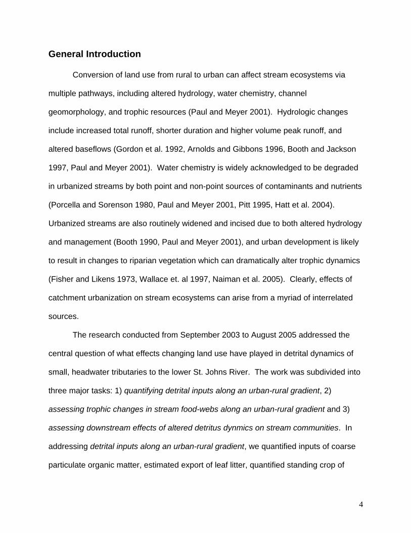
4. Effects of freshwater tidal flow on litter decomposition and

macroinvertebrate community structure in urbanized tributaries of the

lower St. Johns River, Florida

4.1 Introduction…………………………………………..…………… 64

4.2 Methods………………………………………..…………………. 66

4.3 Results and Discussion…………………………………………. 72

4.4 Conclusions……………….……………………………………… 87

4.5 Literature Cited…………………………………………………… 93

4.6 Appendix 2……………………………………………………….. 97

3

General Introduction

Conversion of land use from rural to urban can affect stream ecosystems via

multiple pathways, including altered hydrology, water chemistry, channel

geomorphology, and trophic resources (Paul and Meyer 2001). Hydrologic changes

include increased total runoff, shorter duration and higher volume peak runoff, and

altered baseflows (Gordon et al. 1992, Arnolds and Gibbons 1996, Booth and Jackson

1997, Paul and Meyer 2001). Water chemistry is widely acknowledged to be degraded

in urbanized streams by both point and non-point sources of contaminants and nutrients

(Porcella and Sorenson 1980, Paul and Meyer 2001, Pitt 1995, Hatt et al. 2004).

Urbanized streams are also routinely widened and incised due to both altered hydrology

and management (Booth 1990, Paul and Meyer 2001), and urban development is likely

to result in changes to riparian vegetation which can dramatically alter trophic dynamics

(Fisher and Likens 1973, Wallace et. al 1997, Naiman et al. 2005). Clearly, effects of

catchment urbanization on stream ecosystems can arise from a myriad of interrelated

sources.

The research conducted from September 2003 to August 2005 addressed the

central question of what effects changing land use have played in detrital dynamics of

small, headwater tributaries to the lower St. Johns River. The work was subdivided into

three major tasks: 1) quantifying detrital inputs along an urban-rural gradient, 2)

assessing trophic changes in stream food-webs along an urban-rural gradient and 3)

assessing downstream effects of altered detritus dynmics on stream communities. In

addressing detrital inputs along an urban-rural gradient, we quantified inputs of coarse

particulate organic matter, estimated export of leaf litter, quantified standing crop of

4

benthic organic matter, and measured processing rates for coarse detritus. Trophic

changes along an urban-rural gradient were measured using both functional and

structural assessments of benthic invertebrates. These included preliminary measures

of whole-stream metabolism and stable isotope analysis. Both methods showed

potential to assess the relative importance of autochthonous and allochthonous organic

matter. Assessment of downstream effects was limited to measure of coarse organic

matter export.

The work conducted during the last two years of this funding sought to further

understand the implications of catchment-scale land use changes on the structure and

function of headwater tributaries of the lower St. Johns River. This work was divided

into three areas: 1) metabolism and food web structure in stream reaches with Hydrilla

verticillata, an invasive macrophyte, 2) ammonium uptakes rates in an urbanized,

headwater tributary of the St. Johns River (Mimm’s Creek), and 3) litter decomposition

and benthic macroinvertebrate structure in streams that experience freshwater tidal flow

regimes.

During the course of this work, the southeastern United States (including the

greater Jacksonville area) began a period of below normal rainfall. These drought

conditions resulted in decreases in stream discharge and required several modifications

to the research tasks.

5

Literature Cited

Arnold, C. L., and C. J. Gibbons. 1996. Impervious surface coverage: the emergence of

a key environmental indicator. Journal of the American Planning Association

62:243-258.

Booth, D. B. 1990. Stream-channel incision following drainage-basin urbanization.

Water Resources Bulletin 26:407-417.

Booth, D. B., and C. R. Jackson. 1997. Urbanization of aquatic systems: degradation

thresholds, stormwater detection, and the limits of mitigation. Journal of the

American Water Resources Association 33:1077-1090.

Fisher, S. G., and G. E. Likens. 1973. Energy Flow in Bear Brook, New Hampshire: an

integrative approach to stream ecosystem metabolism. Ecological Monographs

43:421-439.

Gordon, N. D., T. A. McMahon, and B. L. Finlayson. 1992. Stream hydrology: an

introduction for ecologists. Wiley, New York, New York, USA.

Naiman, R.J., H. Décamps, and M. McClain. 2005. Riparia. Academic Press, San

Diego, California, USA

Newell S.Y., T. L. Arsuffi, and R. D. Fallon. 1988. Fundamental procedures for

determining ergosterol content of decaying plant-material by liquid-

chromatography. Applied and Environmental Microbiology 54: 1876-1879

Ourso, R. T., and S. A. Frenzel. 2003. Identification of linear and threshold responses in

streams along a gradient of urbanization in Anchorage, Alaska. Hydrobiologia

501:117-131.

6

Paul, M. J., and J. L. Meyer. 2001. Streams in the urban landscape. Annual Review of

Ecology and Systematics 32:333-365.

Wallace, J. B., S. L. Eggerts, J. L. Meyer, and J. R. Webster. 1997. Multiple trophic

levels of a forest stream linked to terrestrial litter inputs. Science 277:102-104.

7

2. Effects of Hydrilla verticillata, an Invasive Aquatic Macrophyte, on

Stream Metabolism and Food Web Structure.

2.1 Introduction

Due to urban development, forest vegetation from the riparian zone of many

headwater tributaries of the lower St. Johns River Basin has been removed. This

alteration has increased the amount of sunlight received by these streams and

facilitates the establishment of aquatic macrophytes, particularly Hydrilla verticillata (L.

f.) Royle. Hydrilla verticillata is an invasive macrophyte that was introduced to Florida in

the early 1950’s (Schmitz et al. 1991). It spread quickly, likely due to vegetative

reproduction (i.e., regrowth from stem fragments and tubers) and because aquatic

habitats in Florida are excellent for H. verticillata growth. For example, the highest rates

of photosynthesis and most favorable stem growth occurs at temperatures between 16-

24oC (Barko and Smart 1981), which are typical for many northern Florida streams.

Under these conditions, stems can grow several meters per year. However, stems do

senesce if exposed to colder temperatures (Cook and Luond 1982, Carter et al. 1994,

Langland 1996) which can occur for limited periods in the northern St Johns basin. H.

verticillata can also grow at low light levels relative to other macrophytes and stem

elongation (2-6 meters) can occur even when light is near limiting levels (Haller and

Sutton 1975, Barko and Smart 1981). Along with favorable conditions for growth, there

are only a few herbivores in Florida aquatic systems that are known to feed on live H.

verticillata stems, and these have been shown to have little effect on its distribution and

growth (Langland 1996).

8

The introduction and spread of H. verticillata has had a dramatic effect on

headwater tributaries of the St. Johns River. Although the changes brought on by H.

verticillata in stream ecosystems are many, there are two factors that are of particular

concern. First, relatively constant concentrations of dissolved oxygen are changed to

widely fluctuating concentrations, from incipient anoxia during early morning to extreme

supersaturation during afternoon. The effects of such fluctuations on a fauna adapted

to the relatively constant conditions of the originally forested streams have probably

been severe. Second, the source of organic carbon to the streams has shifted from a

predominantly terrestrial origin (riparian leaf litter and dissolved organic carbon) to net

production by autochthonous H. verticillata biomass. The shift of carbon sources from

allochthonous leaf litter to autochthonous living H. verticillata biomass and detritus is

likely to have large effects of stream food webs due to differences in food quality and

seasonal availability. Given the potentially large amount of H. verticillata biomass

produced in streams lacking canopy shading, this carbon source may form an important

subsidy for detritivores.

The goal of this study was to quantify seasonal changes in metabolism and food

web structure in stream reaches with and without Hydrilla verticillata. Our first objective

was to determine how annual variation in H. verticillata affects net ecosystem

metabolism. Based on a preliminary study (Fig. 1), we knew that daily patterns in

oxygen concentrations change dramatically with the introduction of H. verticillata. In the

absence of this macrophyte (i.e., shaded streams), dissolved oxygen concentrations

show little daily fluctuations. When macrophytes are present (e.g., open canopy

streams), dissolved oxygen has wide night- to-day fluctuations and anoxic conditions

9

10

can occur. However, the degree of variation of gross primary production (GPP) and

community respiration (CR) among streams with differing amounts of H. verticillata is

unknown. Also, unknown is how seasonal variations in temperature and subsequent H.

verticillata biomass and detritus affect stream metabolism. Our second objective was to

investigate how autochthonous vs. allochthonous resources affect stream food webs

using stable isotopes of nitrogen and carbon as tracers. Specifically, we wanted to see

if H. verticillata carbon is assimilated by consumers. Finally, we investigated how

spatial and seasonal changes in H. verticillata biomass alters natural abundance

nitrogen and carbon isotope signatures of the abundant taxa that comprise stream food

webs.

Figure 1. Dissolved oxygen concentrations measured at 5 minute intervals over a 48 hour period (23-26 May 2005) in

two headwater tributaries of the St. Johns River (left panel=shaded stream lacking Hydrilla verticillata and 65-66%

saturation; right panel= open canopy stream with H. verticillata present with a range of ~15% saturation during night

to122% during day).

11

2.2 Methods

2.2.1 Study sites

Three streams in the greater Jacksonville, Florida, area were the focus of this

study (Fig. 2). Catchment boundaries and estimates of land cover were provided by the

St. John’s River Water Management District (Fig. 2, Table 1). Total impervious area

was calculated using a normalized difference vegetation index (see Chadwick et al.

2006). Monthly water samples were analyzed for alkalinity (ALK), biological oxygen

demand (BOD), chlorophyll a (Chla), conductivity (CON), dissolved oxygen (DO),

dissolved organic carbon (DOC), ammonium (NH4), nitrate (NO3), total Kjeldahl nitrogen

(TKN), pH, dissolved phosphate (PO4), total dissolved phosphorus (TP), total dissolved

solids (TDS), total suspended solids (TSS), volatile suspended solids (VSS), and a suite

of metals (Al, Cd, Cu, Fe, Mg, Mn, Ni, Pb, Zn). Water was filtered on site and all

samples were analyzed within 24 hours of collection. Water temperature, conductivity,

and dissolved oxygen data were collected using a YSI DO meter. Both the St. Johns

River Water Management District laboratory and contracted laboratories were used for

analysis of the array of water quality constituents. All analyses were performed using

U.S. EPA and Florida Department of Environmental Protection approved methods (40

CFR 100-149, APHA 1998). Current velocities, water depth, and cross-sectional area

were measured in each stream and used to calculate discharge (Q).

In each stream, two 50-meter stream reaches were selected. The upstream

reach lacked forested vegetation and dense stands of H. verticillata were present during

some period of the year. The downstream reach had significant canopy cover and H.

verticillata was absent. All streams had sandy substrata. Riparian canopies, where

12

present, were dominated by red maple (Acer rubrum), sweetgum (Liquidambar

styraciflua), and water oak (Quercus nigra). Because of the low channel gradients,

stream habitats were simple, being composed of runs with occasional coarse woody

snags.

2.2.2 Hydrilla verticillata biomass

Benthic samples were collected in early December 2005, February 2006, July

2006, and October 2006 using a modified Hess sampler (0.07 m2). At each stream, 5

randomly selected locations were selected and a sample was taken in the middle of the

stream channel. The grabs were emptied into a 4 gallon bucket. All H. verticillata

stems were removed by hand and placed in a plastic bag. Samples were either

preserved in the field with ~5% formaldehyde or placed on ice and later frozen.

Collected material was eventually dried to constant mass (60o C), and then weighed. A

portion from each sample was ashed (550o C) and the ash weight was combined with

dry weight to calculate ash free dry mass (AFDM).

2.2.3 Whole-stream metabolism

Respired (CR) and photosynthetically fixed carbon (GPP) was estimated using

the single station dissolved oxygen change technique (Owens 1974, Bott 1996). YSI

600XL Multi-Parameter Water Quality probes were deployed in each reach for at least

24 hours in early December 2005, February 2006, July 2006, and October 2006.

Sample periods were chosen such that water levels were stable (i.e., no storm flow). In

each stream reach dissolved oxygen and temperature was recorded at one minute

13

intervals. Mean dissolved oxygen concentrations were then averaged over 15-min

intervals (i.e., averaged from 1 minute intervals) and corrected for estimated oxygen

reaeration. These records were then analyzed using the single-station night-time

regression method to derive GPP and CR for each 15 minute interval (Owens 1974,

Bott 1996, Fig. 3)

2.2.4 Natural abundance stable isotopes

The relative importance of H. verticillata as a source of carbon and nitrogen to

stream food webs was assessed using stable isotope analysis. One to three replicate

samples (depending on availability) of putative food sources and abundant consumers

were collected quarterly (December 2005, February 2006, June 2006, and October

2006) from the study reaches. Hydrilla verticillata stems, coarse particulate matter

(CPOM), and oxidized coarse particulate organic matter (OCPOM) were collected by

hand. Fine particulate organic matter (FPOM) was collected from depositional area

within the stream using a transfer pipette. Epilithon (epil) was scraped from available

substrate and also rinsed from H. verticillata stems (i.e., epiphyton –epip). Sample were

collected on a pre-ashed glass fiber filters. Invertebrates were collected with a kick net

and by hand from representative habitats in all the reaches. Specimens were

transported to the laboratory on ice and then frozen. Later, specimens were thawed,

cleaned of any detached detritus, and their gut contents removed by dissection (with the

exception of small chironomids). All material was dried at 50°C and finely ground in a

Spex ball mill. Samples were then weighed to ~1 mg for each replicate. Larger taxa

were analyzed individually (e.g. snails, clams, crayfish, dragonflies) while several

14

smaller taxa (e.g., amphipods and midges) were combined to form a single composite

sample. Samples were then sent to the Colorado Plateau Stable Isotope Laboratory at

Northern Arizona University for analysis.

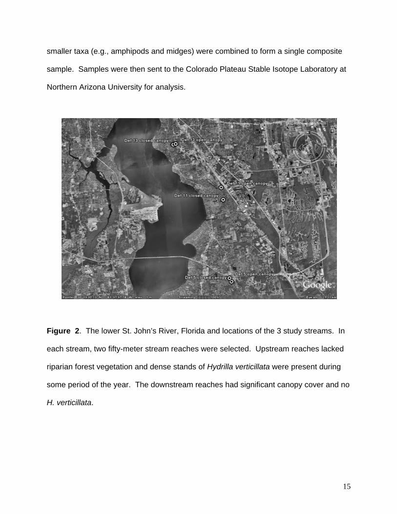
Figure 2. The lower St. John’s River, Florida and locations of the 3 study streams. In

each stream, two fifty-meter stream reaches were selected. Upstream reaches lacked

riparian forest vegetation and dense stands of Hydrilla verticillata were present during

some period of the year. The downstream reaches had significant canopy cover and no

H. verticillata.

15

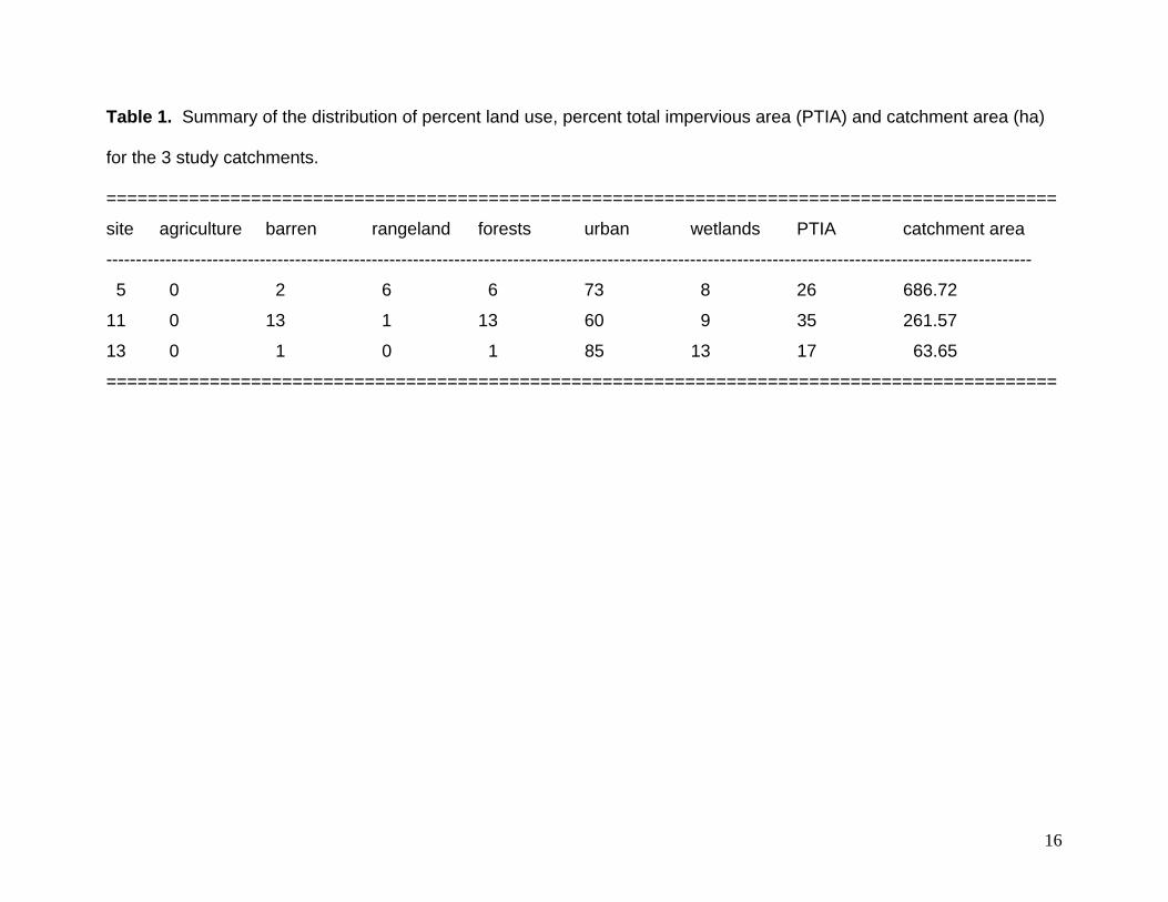
Table 1. Summary of the distribution of percent land use, percent total impervious area (PTIA) and catchment area (ha)

for the 3 study catchments.

============================================================================================

site agriculture barren rangeland forests urban wetlands PTIA catchment area

-------------------------------------------------------------------------------------------------------------------------------------------------------------

5 0 2 6 6 73 8 26 686.72

11 0 13 1 13 60 9 35 261.57

13 0 1 0 1 85 13 17 63.65

============================================================================================

16

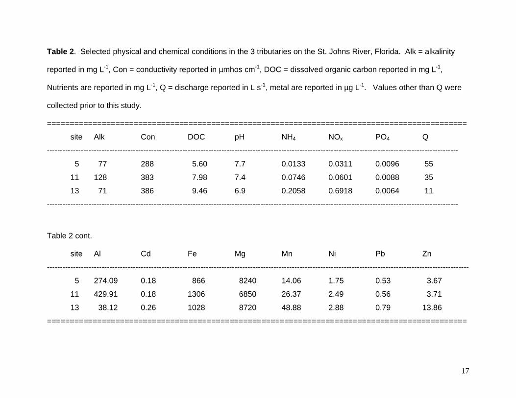
Table 2. Selected physical and chemical conditions in the 3 tributaries on the St. Johns River, Florida. Alk = alkalinity

reported in mg L-1, Con = conductivity reported in µmhos cm-1, DOC = dissolved organic carbon reported in mg L-1,

Nutrients are reported in mg L-1, Q = discharge reported in L s-1, metal are reported in µg L-1. Values other than Q were

collected prior to this study.

============================================================================================

site Alk Con DOC pH NH4 NOx PO4 Q

--------------------------------------------------------------------------------------------------------------------------------------------------------------

5 77 288 5.60 7.7 0.0133 0.0311 0.0096 55

11 128 383 7.98 7.4 0.0746 0.0601 0.0088 35

13 71 386 9.46 6.9 0.2058 0.6918 0.0064 11

--------------------------------------------------------------------------------------------------------------------------------------------------------------

Table 2 cont.

site Al Cd Fe Mg Mn Ni Pb Zn

------------------------------------------------------------------------------------------------------------------------------------------------------------------

5 274.09 0.18 866 8240 14.06 1.75 0.53 3.67

11 429.91 0.18 1306 6850 26.37 2.49 0.56 3.71

13 38.12 0.26 1028 8720 48.88 2.88 0.79 13.86

============================================================================================

17

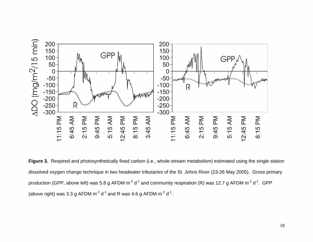
Figure 3. Respired and photosynthetically fixed carbon (i.e., whole-stream metabolism) estimated using the single station

dissolved oxygen change technique in two headwater tributaries of the St. Johns River (23-26 May 2005). Gross primary

production (GPP, above left) was 5.8 g AFDM m-2 d-1 and community respiration (R) was 12.7 g AFDM m-2 d-1. GPP

(above right) was 3.3 g AFDM m-2 d-1 and R was 4.6 g AFDM m-2 d-1.

18

2.3 Results and Discussion

2.3.1 Hydrilla verticillata biomass

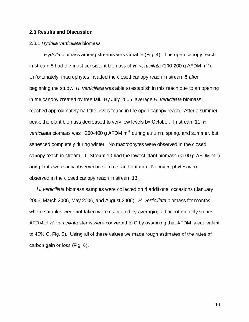
Hydrilla biomass among streams was variable (Fig. 4). The open canopy reach

in stream 5 had the most consistent biomass of H. verticillata (100-200 g AFDM m-2).

Unfortunately, macrophytes invaded the closed canopy reach in stream 5 after

beginning the study. H. verticillata was able to establish in this reach due to an opening

in the canopy created by tree fall. By July 2006, average H. verticillata biomass

reached approximately half the levels found in the open canopy reach. After a summer

peak, the plant biomass decreased to very low levels by October. In stream 11, H.

verticillata biomass was ~200-400 g AFDM m-2 during autumn, spring, and summer, but

senesced completely during winter. No macrophytes were observed in the closed

canopy reach in stream 11. Stream 13 had the lowest plant biomass (<100 g AFDM m-2)

and plants were only observed in summer and autumn. No macrophytes were

observed in the closed canopy reach in stream 13.

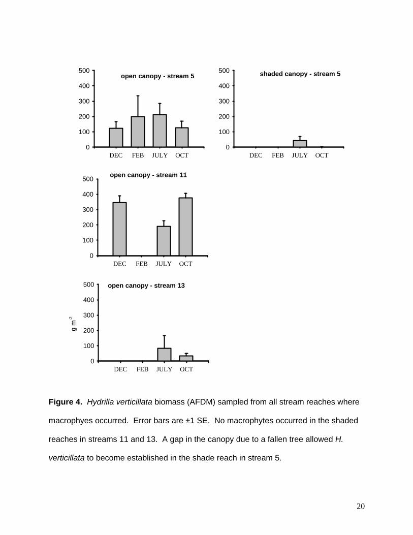
H. verticillata biomass samples were collected on 4 additional occasions (January

2006, March 2006, May 2006, and August 2006). H. verticillata biomass for months

where samples were not taken were estimated by averaging adjacent monthly values.

AFDM of H. verticillata stems were converted to C by assuming that AFDM is equivalent

to 40% C, Fig. 5). Using all of these values we made rough estimates of the rates of

carbon gain or loss (Fig. 6).

19

DEC FEB JULY OCT0

100

200

300

400

500

DEC FEB JULY OCT0

100

200

300

400

500

DEC FEB JULY OCT0

100

200

300

400

500

DEC FEB JULY OCT

g m

-2

0

100

200

300

400

500

open canopy - stream 5 shaded canopy - stream 5

open canopy - stream 11

open canopy - stream 13

Figure 4. Hydrilla verticillata biomass (AFDM) sampled from all stream reaches where

macrophyes occurred. Error bars are ±1 SE. No macrophytes occurred in the shaded

reaches in streams 11 and 13. A gap in the canopy due to a fallen tree allowed H.

verticillata to become established in the shade reach in stream 5.

20

DEC JAN FEB MAR APR MAY JUNE JULY AUG SEP OCT

0

50

100

150

200

250

300 Stream 5 open canopyStream 5 shaded canopyStream 11 open canopyStream 13 open canopy

g C

m-2

**

*

+ ++

+

*+ additional samples

estimated

Figure 5. Summary of all H. verticillata biomass samples collected (January 2006, March 2006, May 2006, and August

2006) and estimated biomass for months where samples were not taken (April 2006 and June 2006).

21

22

Figure 6. Monthly estimates of carbon gains or losses for Hydrilla verticillata biomass from all stream reaches.

DEC JAN FEB MAR APR MAY JUNE JULY AUG SEP

g C

m- 2

d-1

-6

-4

-2

0

2

4

6 Stream 5 open canopyStream 5 shaded canopyStream 11 open canopyStream 13 open canopy

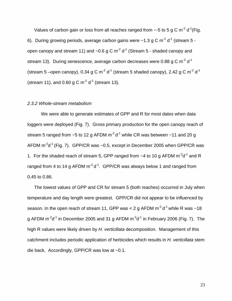
Values of carbon gain or loss from all reaches ranged from ~-5 to 5 g C m-2 d-1(Fig.

6). During growing periods, average carbon gains were ~1.3 g C m-2 d-1 (stream 5 -

open canopy and stream 11) and ~0.6 g C m-2 d-1 (Stream 5 - shaded canopy and

stream 13). During senescence, average carbon decreases were 0.88 g C m-2 d-1

(stream 5 –open canopy), 0.34 g C m-2 d-1 (stream 5 shaded canopy), 2.42 g C m-2 d-1

(stream 11), and 0.60 g C m-2 d-1 (stream 13).

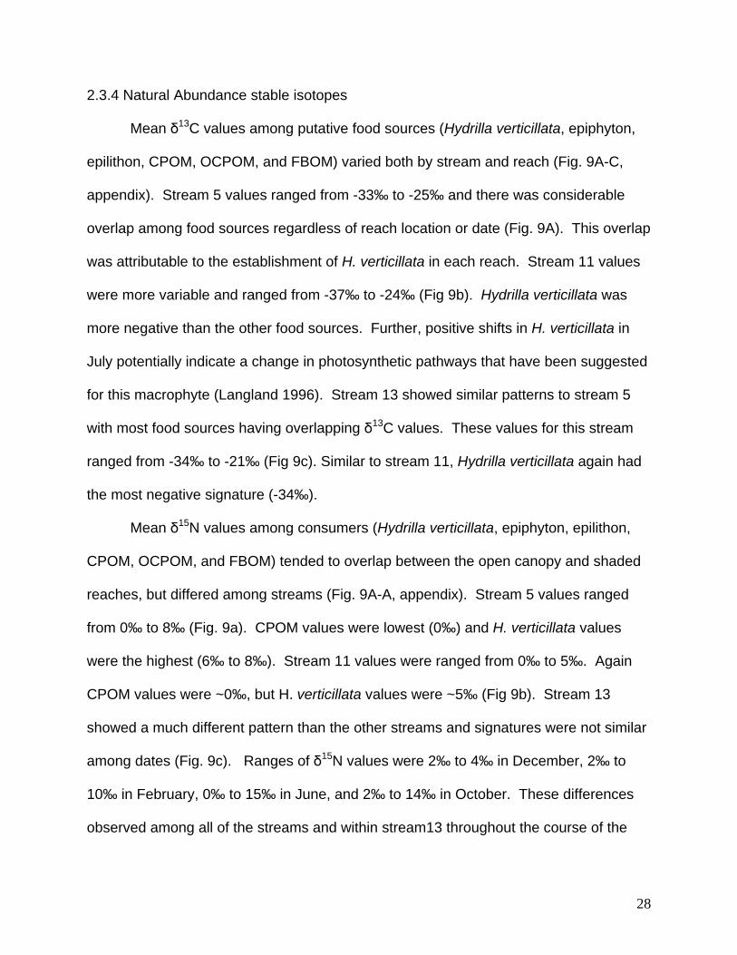
2.3.2 Whole-stream metabolism

We were able to generate estimates of GPP and R for most dates when data

loggers were deployed (Fig. 7). Gross primary production for the open canopy reach of

stream 5 ranged from ~5 to 12 g AFDM m-2 d-1 while CR was between ~11 and 20 g

AFDM m-2d-1 (Fig. 7). GPP/CR was ~0.5, except in December 2005 when GPP/CR was

1. For the shaded reach of stream 5, GPP ranged from ~4 to 10 g AFDM m-2d-1 and R

ranged from 4 to 14 g AFDM m-2 d-1. GPP/CR was always below 1 and ranged from

0.45 to 0.86.

The lowest values of GPP and CR for stream 5 (both reaches) occurred in July when

temperature and day length were greatest. GPP/CR did not appear to be influenced by

season. In the open reach of stream 11, GPP was < 2 g AFDM m-2 d-1 while R was ~18

g AFDM m-2d-1 in December 2005 and 31 g AFDM m-2d-1 in February 2006 (Fig. 7). The

high R values were likely driven by H. verticillata decomposition. Management of this

catchment includes periodic application of herbicides which results in H. verticillata stem

die back. Accordingly, GPP/CR was low at ~0.1.

23

Metabolism was not estimated in July 2006 and October 2006 in the open reach of

stream 11 due to anoxia. GPP during these periods, however, was likely high given the

amount of biomass that accrued during these periods. If the maximum rate of H.

verticillata carbon gain (~5 g C m-2 d-1 or 13 g AFDM m-2 d-1, Fig. 6) is assumed to be

equivalent to net primary production (NPP) and GPP = NPP/0.556, then GPP could be

as high as ~22 g AFDM m-2 d-1 for H. verticillata alone (e.g., not including epiphytic and

epilithic biofilms). In the shaded reach, GPP was also < 2 g AFDM m-2d-1, but CR

ranged from ~6 to 8 g AFDM m-2 d-1 (Fig. 7). GPP/CR ranged from 0.1 to 0.3.

In stream 13 both data logger failure and anoxia prevented estimates of ecosystem

metabolism for some dates. In the open canopy reach GPP varied from ~5 to 8 g AFDM

m-2 d-1 while CR was from ~6 to 29 g AFDM m-2 d-1. GPP/CR ranged from 0.4 to 0.8. In

the shaded canopy, GPP was <2 and CR was ~6 g AFDM m-2 d-1. GPP/CR was 0.23 in

July 2006 and 0.03 in October 2006.

Both GPP and CR tended to be lower in the shaded reaches as would be expected.

In the open canopy reaches, metabolism was influenced by the dynamics of H.

verticillata growth and senescence. The open canopy reaches were autotrophic (i.e.,

GPP/CR>1) for short periods when photosynthetic rates were maximized. Overall,

however, these reaches were highly heterotrophic (except stream 5 in December 2005).

For example, respiration in stream 11 in the open canopy reach required 31 g AFDM m-

2 d-1 while the total amount of organic matter produced by photosynthesis was only 2.5 g

AFDM m-2 d-1 . Presumably the greater levels of respiration are related to stores of H.

verticillata biomass, detritus, and smaller fractions of allochthonous organic matter. The

lack of balance between GPP and CR clearly indicates that consumers require

24

supplemental sources (e.g., particulate or dissolved organic matter) to support their

metabolic activity.

Estimates of GPP and CR using whole-system methods are complicated by fluxes of

dissolved oxygen to and from the atmosphere (reaeration). The direction of flux is

dependant on the level of oxygen saturation in the stream. Our estimates of reaeration

using nighttime regression (Fig. 8; 0.001 to 0.092 min-1, Owens 1974) were similar to

those calculated using a tracer gas methods (Marzolf et al. 1994) in low gradient

streams in southwestern Georgia (Mulholland et al. 2005). We attempted to calculate

reaeration using the same technique (Marzolf et al. 1994), but found highly variable

levels of tracer gas concentration suggesting that we injected the tracer gas (propane)

too close to the study reach resulting in incomplete mixing at the upstream sampling

location.

25

DEC FEB JULY OCT0

5

10

15

20

25

30

35

DEC FEB JULY OCT0

5

10

15

20

25

30

35

DEC FEB JULY OCT0

5

10

15

20

25

3035

DEC FEB JULY OCT0

5

10

15

20

25

3035

DEC FEB JULY OCT0

5

10

15

20

25

3035

DEC FEB JULY OCT

gC m

-2 d

-1

0

5

10

15

20

25

30

35

open canopy shaded canopy

stream 5

stream 11

stream 13

A A

LF LF WL

gC m

-2 d

-1gC

m-2

d-1

GPPR

Figure 7. Gross primary production (GPP) and community respiration (R) estimated

using the single station dissolved oxygen change technique. A = anoxic conditions, LF

= logger failure, WL= unstable water level.

26

rearation min-10.00 0.02 0.04 0.06 0.08 0.10

(g C

m-2

d-1

)

0

5

10

15

20

25

30

35

GPPR

Figure 8. Estimated reaeration using nighttime regression methods.

27

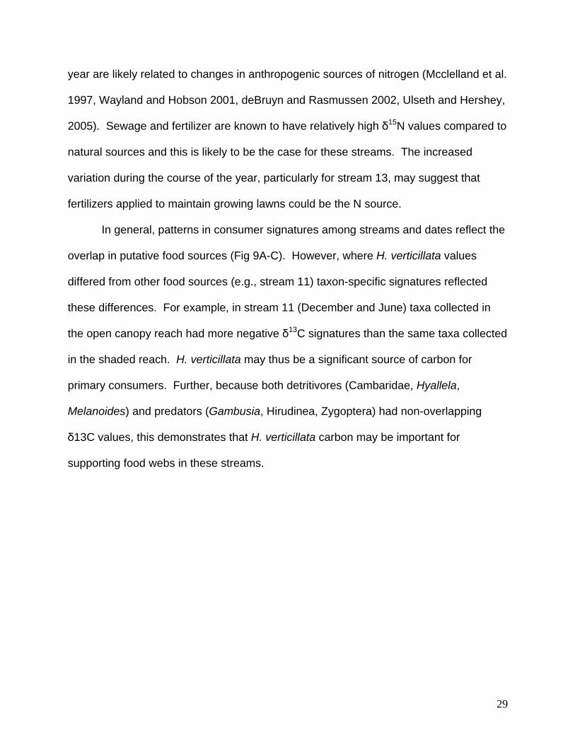
2.3.4 Natural Abundance stable isotopes

Mean δ13C values among putative food sources (Hydrilla verticillata, epiphyton,

epilithon, CPOM, OCPOM, and FBOM) varied both by stream and reach (Fig. 9A-C,

appendix). Stream 5 values ranged from -33‰ to -25‰ and there was considerable

overlap among food sources regardless of reach location or date (Fig. 9A). This overlap

was attributable to the establishment of H. verticillata in each reach. Stream 11 values

were more variable and ranged from -37‰ to -24‰ (Fig 9b). Hydrilla verticillata was

more negative than the other food sources. Further, positive shifts in H. verticillata in

July potentially indicate a change in photosynthetic pathways that have been suggested

for this macrophyte (Langland 1996). Stream 13 showed similar patterns to stream 5

with most food sources having overlapping δ13C values. These values for this stream

ranged from -34‰ to -21‰ (Fig 9c). Similar to stream 11, Hydrilla verticillata again had

the most negative signature (-34‰).

Mean δ15N values among consumers (Hydrilla verticillata, epiphyton, epilithon,

CPOM, OCPOM, and FBOM) tended to overlap between the open canopy and shaded

reaches, but differed among streams (Fig. 9A-A, appendix). Stream 5 values ranged

from 0‰ to 8‰ (Fig. 9a). CPOM values were lowest (0‰) and H. verticillata values

were the highest (6‰ to 8‰). Stream 11 values were ranged from 0‰ to 5‰. Again

CPOM values were ~0‰, but H. verticillata values were ~5‰ (Fig 9b). Stream 13

showed a much different pattern than the other streams and signatures were not similar

among dates (Fig. 9c). Ranges of δ15N values were 2‰ to 4‰ in December, 2‰ to

10‰ in February, 0‰ to 15‰ in June, and 2‰ to 14‰ in October. These differences

observed among all of the streams and within stream13 throughout the course of the

28

29

year are likely related to changes in anthropogenic sources of nitrogen (Mcclelland et al.

1997, Wayland and Hobson 2001, deBruyn and Rasmussen 2002, Ulseth and Hershey,

2005). Sewage and fertilizer are known to have relatively high δ15N values compared to

natural sources and this is likely to be the case for these streams. The increased

variation during the course of the year, particularly for stream 13, may suggest that

fertilizers applied to maintain growing lawns could be the N source.

In general, patterns in consumer signatures among streams and dates reflect the

overlap in putative food sources (Fig 9A-C). However, where H. verticillata values

differed from other food sources (e.g., stream 11) taxon-specific signatures reflected

these differences. For example, in stream 11 (December and June) taxa collected in

the open canopy reach had more negative δ13C signatures than the same taxa collected

in the shaded reach. H. verticillata may thus be a significant source of carbon for

primary consumers. Further, because both detritivores (Cambaridae, Hyallela,

Melanoides) and predators (Gambusia, Hirudinea, Zygoptera) had non-overlapping

δ13C values, this demonstrates that H. verticillata carbon may be important for

supporting food webs in these streams.

-38 -36 -34 -32 -30 -28 -26 -24 -22 -20

-2

0

2

4

6

8

10

12

HydepiFBOM

CPOM

HydFBOMFA

LD

FGC

I

H

N

V

L

D FGI

M

K

UV

Dec 2005

-38 -36 -34 -32 -30 -28 -26 -24 -22 -20

-2

0

2

4

6

8

10

12

CPOM

HydepipFBOM

CPOM

FBOML

DGCM

K

NS

V

LDFGC

I

M

K

SV

Feb 2006

-36 -34 -32 -30 -28 -26 -24 -22 -20

-2

0

2

4

6

8

10

12

OCPOM

HydFBOMFBOM

L B

D

FG

I

M

KP

VL

C

D

G

I

M

KNV

June 2006

-38 -36 -34 -32 -30 -28 -26 -24 -22 -20

-2

0

2

4

6

8

10

12

epilFBOM

CPOM

epil FBOML

Q

BCD

GI

P

V LB

CD

G

I

MN

E

V

Oct 2006

Figure 9a. Average δ13C and δ15 N values for putative food sources and consumers for stream 5 in December 2005,

February 2006, June 2006, and October 2006. Error bars are ±1 SE. Taxon names associated with each letter are found

in the appendix.

30

-44 -42 -40 -38 -36 -34 -32 -30 -28 -26 -24-2

0

2

4

6

8

10

12

HydepipFBOMCPOM

FBOML

Q RD

I

J

H

NAV

LC

DGIK

N

E

U

V

Dec 2005

-44 -42 -40 -38 -36 -34 -32 -30 -28 -26 -24-2

0

2

4

6

8

10

12

Hyd FBOM

CBOM

FBOMLC

DF

I

J

K

N

A

T

L

B

C

DFG

I

M

K

S

E

V

Feb 2006

-42 -40 -38 -36 -34 -32 -30 -28 -26-2

0

2

4

6

8

10

12

CPOM

HydEpil FBOM

CPOMOPOMEpilFBOML

QDF

I

J

K

AV

L

BDG

I

M

K

NV

June 2006

-44 -42 -40 -38 -36 -34 -32 -30 -28 -26 -24-2

0

2

4

6

8

10

12

CPOMepil

FBOM

CPOMFBOM

L

B D

F

I

J

K

PA

L

Q

FG

N

PV

Oct 2006

Figure 9b. Average δ13C and δ15 N values for putative food sources and consumers for stream 11 in December 2005,


in the appendix..

31

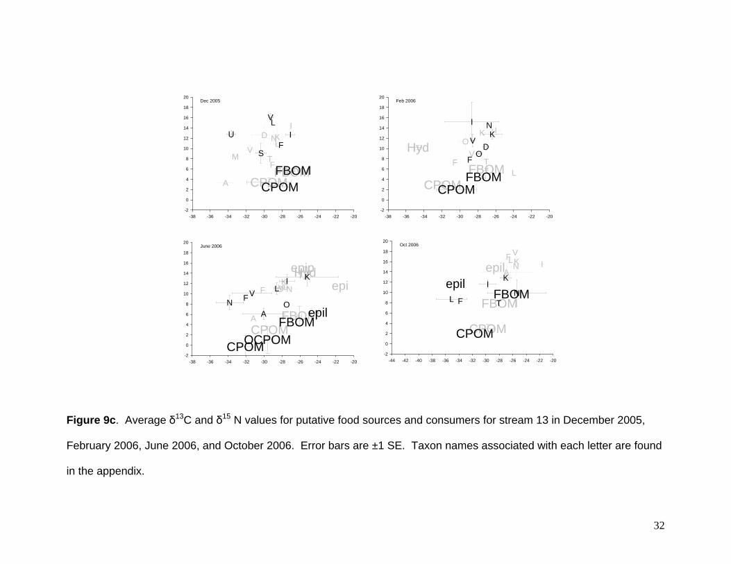
Figure 9c. Average δ13C and δ15 N values for putative food sources and consumers for stream 13 in December 2005,


in the appendix.

32

-38 -36 -34 -32 -30 -28 -26 -24 -22 -20-2

0

2

4

6

8

10

12

14

16

18

20

CPOMFBOM

CPOMFBOM

LD

F

I

M

KN

A

TV

L

FI

S

U

V

Dec 2005

-38 -36 -34 -32 -30 -28 -26 -24 -22 -20-2

0

2

4

6

8

10

12

14

16

18

20

CPOM

Hyd

FBOMCPOM

FBOM LF

IKO

TV

DF

IK

N

OV

Feb 2006

-38 -36 -34 -32 -30 -28 -26 -24 -22 -20-2

0

2

4

6

8

10

12

14

16

18

20

CPOM

Hydepipepi

FBOM

CPOMOCPOM

epilFBOM

LF

IK

NO

A

VLF

I K

N OA

V

June 2006

-44 -42 -40 -38 -36 -34 -32 -30 -28 -26 -24 -22 -20-2

0

2

4

6

8

10

12

14

16

18

20

CPOM

epil

FBOM

CPOM

epilFBOM

LF IKNA

V

L F

IK

NT

Oct 2006

2.4 Conclusions

The establishment of H. verticillata, driven by the removal of riparian trees, leads

to dramatic changes in the chemical conditions of these streams. In fact, where H.

verticillata biomass was the greatest anoxic conditions developed for extended periods.

The macrophyte also greatly increases gross primary production, but the streams

continue to have net heterotrophic conditions. This suggests potential carbon limitation

can arise in reaches where H. verticillata is present, especially given the removal of

other allochthonous carbon sources. Further, the establishment of H. verticillata in

stream reaches leads to increased levels of community respiration and clearly

macrophyte detritus fuels this activity. Natural abundance stable isotopes showed that

H. verticillata derived carbon was present in the food webs of open canopy reaches.

Unlike natural abundance carbon found in consumers, H. verticillata did not appear to

alter nitrogen dynamics and this is likely related to the fact that nitrogen signatures are

influenced by anthropogenic sources that change based on the type and degree of

urban development.

Unlike our past work (Chadwick et al. 2006) where urbanization at the catchment

–scale influenced ecosystem function (litter decomposition), this work shows that

ecosystem function (metabolism) is affected by urban development at reach-scales.

Potentially, degradation to streams where H. verticillata is not present could be avoided

and restoration of channels where it is present could be achieved via riparian

management that preserves vegetation that shades stream channels.

33

2.5 Literature Cited

APHA. 1998. Standard Methods for the Examination of Water and Waste Water, 20th

Edition. American Public Health Association, Washington D.C., USA.

Barko, J.W., and R.M. Smart. 1981. Comparative influences of light and temperature on

the growth and metabolism of selected submersed freshwater macrophytes.

Ecological Monographs 51:219-235.

Bott, T.L. 1996. Primary productivity and community respiration. Pages 533–556 in F.

R. Hauer and G. A. Lamberti (editors). Methods in stream ecology. Academic

Press, San Diego, California.

Carter, V., N.B. Rybicki, J.M. Landweh and M. Turtora. 1994. Role of weather and

water quality in population dynamics of submersed macrophytes in the tidal

Potomac River. Estuaries 17:417-426.

Chadwick, M.A., D.R. Dobberfuhl, A.C. Benke, A.D. Huryn, K. Suberkropp, and J. E.

Thiele. 2006. Urbanization affects stream ecosystem function by altering

hydrology, chemistry, and biotic richness. Ecological Applications 16:1796-1807.

Cook, C.D.K., and R. Luond. 1982. A revision of the genus Hydrilla (Hydrocharitaceae).

Aquatic Botany 13:485-504.

DeBruyn, A.M.H., and J.B. Rasmussen. 2007. Quantifying assimilation of sewage-

derived organic matter by river benthos. Ecological Applications 12: 511-520.

Fry, B. 1991. Stable isotope diagrams of freshwater food webs. Ecology 72: 2293-

2297.

34

Grimm, N.B., and S.G. Fischer. 1984. Exchange between interstitial and surface water:

implications for stream metabolism and nutrient cycling. Hydrobiologia 111:219–

228.

Haller, W.T., and D.L. Sutton. 1975. Community structure and competition between

Hydrilla and Vallisneria. Hyacinth Control Journal 13:48-50.

Hoeinghaus, D.J., K.O. Winemiller and A.A. Agostinho, 2007. , Landscape-scale

hydrologic characteristics differentiate patterns of carbon flow in large-river food

webs. Ecosystems 10: 1019-1033.

Huryn, A.D., Riley R., Young R.G., Peacock K. and Arbuckle C.J. 2002. Natural-

abundance stable C and N isotopes indicate weak upstream-downstream linkage

of consumer food webs in a river-floodplain system. Archiv für Hydrobiologie

153:177-196.

Kaenel, B.R., H. Buehrer and U. Uehlinger. 2000. Effects of aquatic plant management

on stream metabolism and oxygen balance in streams. Freshwater Biology 45:

85–95.

Langeland, K.A. 1996. Hydrilla verticillata (L.F.) Royle (Hydrocharitaceae), "The perfect

aquatic weed." Castanea 61: 293-304.

Marzolf, E.R., Mulholland P.J. and Steinman A.D. (1994) Improvements to the diurnal

upstream–downstream dissolved-oxygen change technique for determining

whole-stream metabolism in small streams. Canadian Journal of Fisheries and

Aquatic Sciences, 51, 1591–1599.

35

McClelland, J.W., I. Valiela and R.H. Michener. 1997. Nitrogen-stable isotope

signatures in estuarine food webs: a record of increasing urbanization in coastal

watersheds. Limnology and Oceanography 42:930-937.

Molla, S., L. Maltchik, C. Casado and C. Montes, C. 1996. Particulate organic matter

and ecosystem metabolism dynamics in a temporary Mediterranean stream

Archiv fur Hydrobiologie. 137: 59-76.

Mulholland, P.J., E.R. Marzolf, J.R. Webster, D.R. Hart, and S.P. Hendricks. 1997.

Evidence that hyporheic zones increase heterotrophic metabolism and

phosphorus uptake in forest streams. Limnology and Oceanography. 42:443-451.

Mulholland, P.J., J.N. Houser, and K.O. Maloney. 2005. Stream diurnal dissolved

oxygen profiles as indicators of in-stream metabolism and disturbance effects:

Fort Benning as a case study. Ecological Indicators 5:243-252.

Owens, M. 1974. Measurements on non-isolated natural communities in running waters.

pp. 111-119 in Vollenweider RA (ed.) A manual on methods for measuring

primary production aquatic environments. Blackwell Scientific Publications,

Oxford.

Peterson, B.J., and B. Fry. 1987. Stable isotopes in ecosystem studies. Annual

Review of Ecology and Systematics 18:293–320.

Schmitz D.C., B.V. Nelson, L.E. Nall and J.D. Schardt. 1991. Exotic aquatic plants in

Florida: A historical perspective and review of the present aquatic plant

regulation program. (Online)

36

37

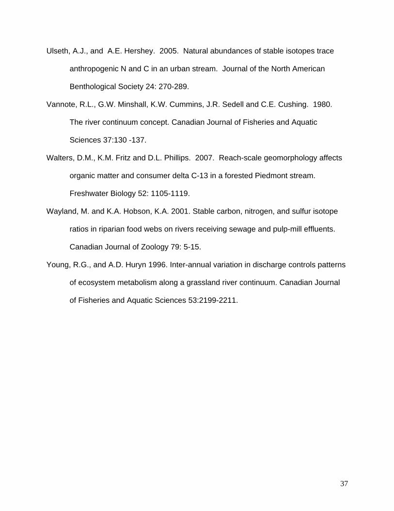
Ulseth, A.J., and A.E. Hershey. 2005. Natural abundances of stable isotopes trace

anthropogenic N and C in an urban stream. Journal of the North American

Benthological Society 24: 270-289.

Vannote, R.L., G.W. Minshall, K.W. Cummins, J.R. Sedell and C.E. Cushing. 1980.

The river continuum concept. Canadian Journal of Fisheries and Aquatic

Sciences 37:130 -137.

Walters, D.M., K.M. Fritz and D.L. Phillips. 2007. Reach-scale geomorphology affects

organic matter and consumer delta C-13 in a forested Piedmont stream.

Freshwater Biology 52: 1105-1119.

Wayland, M. and K.A. Hobson, K.A. 2001. Stable carbon, nitrogen, and sulfur isotope

ratios in riparian food webs on rivers receiving sewage and pulp-mill effluents.

Canadian Journal of Zoology 79: 5-15.

Young, R.G., and A.D. Huryn 1996. Inter-annual variation in discharge controls patterns

of ecosystem metabolism along a grassland river continuum. Canadian Journal

of Fisheries and Aquatic Sciences 53:2199-2211.

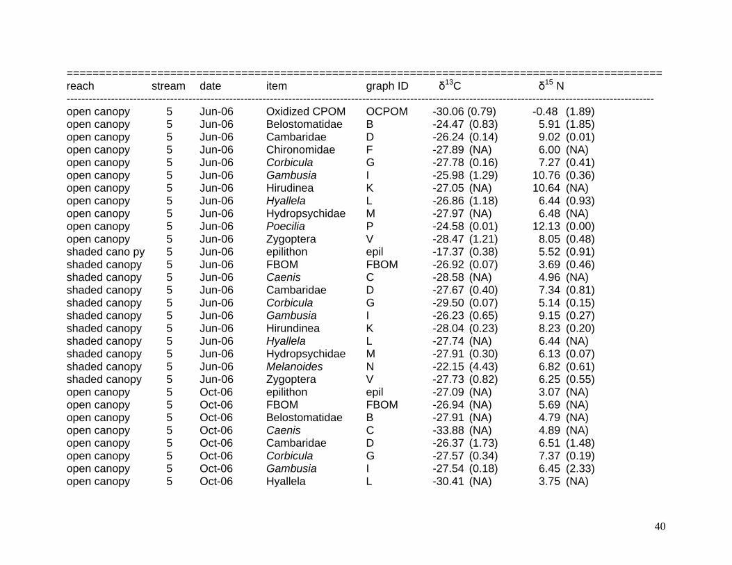
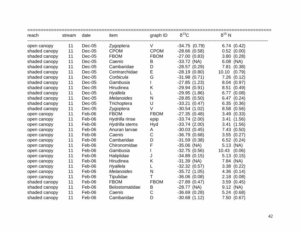
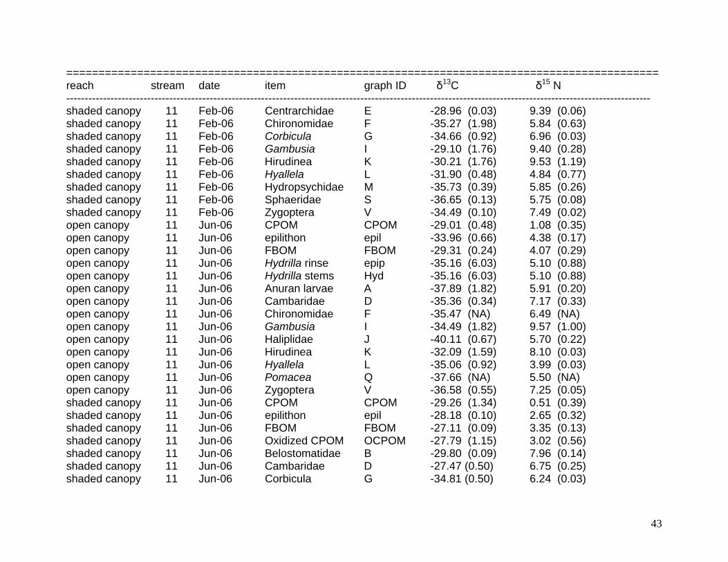
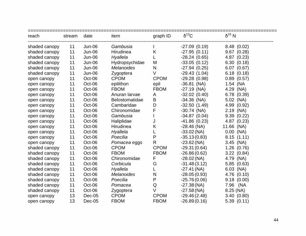
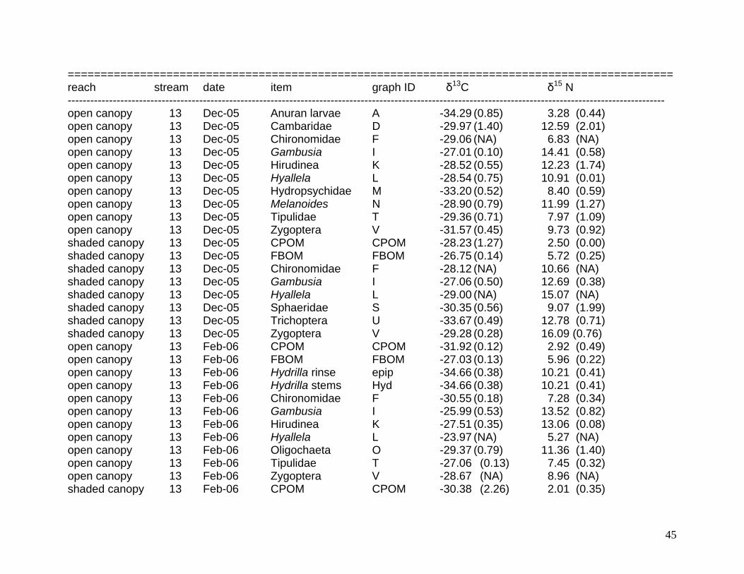
2.6 Appendix 1

Average δ13C and δ15 N values for putative food sources and consumers. Standard errors are reported parenthetically.

============================================================================================ reach stream date item graph ID δ13C δ15 N --------------------------------------------------------------------------------------------------------------------------------------------------------------- open canopy 5 Dec-05 FBOM FBOM -26.87 (0.08) 5.03 (0.14) open canopy 5 Dec-05 Hydrilla rinse epip -29.49 (0.29) 7.80 (0.26) open canopy 5 Dec-05 Hydrilla stems Hyd -29.49 (0.29) 7.80 (0.26) open canopy 5 Dec-05 Caenis C -30.30 (NA) 6.18 (NA) open canopy 5 Dec-05 Cambaridae D -26.44 (2.00) 8.26 (0.80) open canopy 5 Dec-05 Chironomidae F -29.20 (NA) 7.12 (NA) open canopy 5 Dec-05 Corbicula G -29.00 (0.17) 6.80 (0.27) open canopy 5 Dec-05 Fundulus H -30.96 (0.04) 8.05 (0.25) open canopy 5 Dec-05 Gambusia I -24.04 (1.31) 10.56 (0.01) open canopy 5 Dec-05 Hyallela L -27.97 (0.36) 6.79 (0.11) open canopy 5 Dec-05 Melanoides N -29.19 (1.86) 5.67 (0.39) open canopy 5 Dec-05 Zygoptera V -29.20 (0.67) 7.93 (0.27) shaded canopy 5 Dec-05 CPOM CPOM -29.34 (0.68) 1.93 (0.45) shaded canopy 5 Dec-05 FBOM FBOM -27.65 (0.13) 3.60 (0.16) shaded canopy 5 Dec-05 Filamentous algae FA -33.76 (2.31) 3.93 (0.29) shaded canopy 5 Dec-05 Hydrilla rinse epip -31.34 (0.51) 6.36 (0.23) shaded canopy 5 Dec-05 Hydrilla stems Hyd -31.34 (0.51) 6.36 (0.23) shaded canopy 5 Dec-05 Cambaridae D -29.84 (0.66) 7.11 (0.66) shaded canopy 5 Dec-05 Chironomidae F -26.18 (NA) 6.78 (NA) shaded canopy 5 Dec-05 Corbicula G -29.83 (0.78) 6.03 (0.39) shaded canopy 5 Dec-05 Gambusia I -30.07 (NA) 7.96 (NA) shaded canopy 5 Dec-05 Hirudinea K -31.57 (1.30) 7.90 (0.58) shaded canopy 5 Dec-05 Hyallela L -31.36 (0.62) 5.13 (0.39) shaded canopy 5 Dec-05 Hydropsychidae M -35.53 (0.46) 5.63 (0.36) shaded canopy 5 Dec-05 Trichoptera U -35.77 (1.36) 5.71 (0.50)

38

============================================================================================ reach stream date item graph ID δ13C δ15 N --------------------------------------------------------------------------------------------------------------------------------------------------------------- shaded canopy 5 Dec-05 Zygoptera V -32.79 (1.13) 6.59 (0.40) open canopy 5 Feb-06 CPOM CPOM -28.13 (0.78) -1.40 (1.10) open canopy 5 Feb-06 FBOM FBOM -26.20 (0.09) 5.68 (0.08) open canopy 5 Feb-06 Hydrilla rinse epip -28.83 (0.17) 6.56 (0.05) open canopy 5 Feb-06 Hydrilla rinse epip -29.19 (0.57) 8.38 (0.53) open canopy 5 Feb-06 Hydrilla stems Hyd -29.19 (0.57) 8.38 (0.53) open canopy 5 Feb-06 Caenis C -30.28 (NA) 7.25 (NA) open canopy 5 Feb-06 Cambaridae D -27.59 (0.32) 8.87 (0.46) open canopy 5 Feb-06 Corbicula G -29.27 (0.27) 6.99 (0.26) open canopy 5 Feb-06 Hirudinea K -27.27 (NA) 10.77 (NA) open canopy 5 Feb-06 Hyallela L -28.62 (0.12) 6.73 (0.30) open canopy 5 Feb-06 Hydropsychidae M -32.00 (1.04) 7.84 (0.08) open canopy 5 Feb-06 Melanoides N -29.92 (0.22) 8.00 (0.26) open canopy 5 Feb-06 Sphaeridae S -29.03 (NA) 6.89 (NA) open canopy 5 Feb-06 Zygoptera V -28.90 (1.13) 9.13 (0.20) shaded canopy 5 Feb-06 CPOM CPOM -30.79 (0.66) - 0.09 (0.60) shaded canopy 5 Feb-06 FBOM FBOM -27.62 (0.61) 4.32 (0.31) shaded canopy 5 Feb-06 Caenis C -29.87 (0.72) 6.58 (0.27) shaded canopy 5 Feb-06 Cambaridae D -27.58 (0.25) 7.20 (0.14) shaded canopy 5 Feb-06 Chironomidae F -29.56 (NA) 6.60 (NA) shaded canopy 5 Feb-06 Corbicula G -30.26 (0.04) 6.28 (0.26) shaded canopy 5 Feb-06 Gambusia I -27.74 (0.80) 9.38 (0.35) shaded canopy 5 Feb-06 Hirudinea K -27.99 (NA) 9.30 (NA) shaded canopy 5 Feb-06 Hyallela L -28.38 (0.21) 5.55 (0.21) shaded canopy 5 Feb-06 Hydropsychidae M -32.23 (0.42) 6.91 (0.23) shaded canopy 5 Feb-06 Sphaeridae S -28.57 (NA) 6.65 (NA) shaded canopy 5 Feb-06 Zygoptera V -29.32 (0.42) 7.70 (0.54) open canopy 5 Jun-06 FBOM FBOM -26.24 (0.35) 4.58 (0.17) open canopy 5 Jun-06 Hydrilla rinse epip -25.16 (1.92) 6.29 (1.73) open canopy 5 Jun-06 Hydrilla stems Hyd -25.16 (1.92) 6.29 (1.73)

39

============================================================================================ reach stream date item graph ID δ13C δ15 N --------------------------------------------------------------------------------------------------------------------------------------------------------------- open canopy 5 Jun-06 Oxidized CPOM OCPOM -30.06 (0.79) -0.48 (1.89) open canopy 5 Jun-06 Belostomatidae B -24.47 (0.83) 5.91 (1.85) open canopy 5 Jun-06 Cambaridae D -26.24 (0.14) 9.02 (0.01) open canopy 5 Jun-06 Chironomidae F -27.89 (NA) 6.00 (NA) open canopy 5 Jun-06 Corbicula G -27.78 (0.16) 7.27 (0.41) open canopy 5 Jun-06 Gambusia I -25.98 (1.29) 10.76 (0.36) open canopy 5 Jun-06 Hirudinea K -27.05 (NA) 10.64 (NA) open canopy 5 Jun-06 Hyallela L -26.86 (1.18) 6.44 (0.93) open canopy 5 Jun-06 Hydropsychidae M -27.97 (NA) 6.48 (NA) open canopy 5 Jun-06 Poecilia P -24.58 (0.01) 12.13 (0.00) open canopy 5 Jun-06 Zygoptera V -28.47 (1.21) 8.05 (0.48) shaded cano py 5 Jun-06 epilithon epil -17.37 (0.38) 5.52 (0.91) shaded canopy 5 Jun-06 FBOM FBOM -26.92 (0.07) 3.69 (0.46) shaded canopy 5 Jun-06 Caenis C -28.58 (NA) 4.96 (NA) shaded canopy 5 Jun-06 Cambaridae D -27.67 (0.40) 7.34 (0.81) shaded canopy 5 Jun-06 Corbicula G -29.50 (0.07) 5.14 (0.15) shaded canopy 5 Jun-06 Gambusia I -26.23 (0.65) 9.15 (0.27) shaded canopy 5 Jun-06 Hirundinea K -28.04 (0.23) 8.23 (0.20) shaded canopy 5 Jun-06 Hyallela L -27.74 (NA) 6.44 (NA) shaded canopy 5 Jun-06 Hydropsychidae M -27.91 (0.30) 6.13 (0.07) shaded canopy 5 Jun-06 Melanoides N -22.15 (4.43) 6.82 (0.61) shaded canopy 5 Jun-06 Zygoptera V -27.73 (0.82) 6.25 (0.55) open canopy 5 Oct-06 epilithon epil -27.09 (NA) 3.07 (NA) open canopy 5 Oct-06 FBOM FBOM -26.94 (NA) 5.69 (NA) open canopy 5 Oct-06 Belostomatidae B -27.91 (NA) 4.79 (NA) open canopy 5 Oct-06 Caenis C -33.88 (NA) 4.89 (NA) open canopy 5 Oct-06 Cambaridae D -26.37 (1.73) 6.51 (1.48) open canopy 5 Oct-06 Corbicula G -27.57 (0.34) 7.37 (0.19) open canopy 5 Oct-06 Gambusia I -27.54 (0.18) 6.45 (2.33) open canopy 5 Oct-06 Hyallela L -30.41 (NA) 3.75 (NA)

40

============================================================================================ reach stream date item graph ID δ13C δ15 N --------------------------------------------------------------------------------------------------------------------------------------------------------------- open canopy 5 Oct-06 Hyallela L -29.37 (0.82) 6.10 (1.03) open canopy 5 Oct-06 Poecilia P -28.43 (2.22) 8.79 (1.33) open canopy 5 Oct-06 Pomacea Q -29.83 (NA) 7.88 (NA) open canopy 5 Oct-06 Zygoptera V -31.38 (0.31) 6.07 (0.05) shaded canopy 5 Oct-06 CPOM CPOM -29.82 (0.74) 0.26 (0.13) shaded canopy 5 Oct-06 epilithon epil -29.56 (NA) 5.72 (NA) shaded canopy 5 Oct-06 FBOM FBOM -25.80 (NA) 5.09 (NA) shaded canopy 5 Oct-06 Belostomatidae B -26.11 (NA) 7.73 (NA) shaded canopy 5 Oct-06 Caenis C -32.84 (NA) 5.86 (NA) shaded canopy 5 Oct-06 Cambaridae D -29.13 (0.34) 6.81 (0.37) shaded canopy 5 Oct-06 Centrarchidae E -26.43 (NA) 9.68 (NA) shaded canopy 5 Oct-06 Corbicula G -28.34 (0.12) 5.72 (0.12) shaded canopy 5 Oct-06 Gambusia I -25.51 (1.02) 9.10 (0.34) shaded canopy 5 Oct-06 Hyallela L -27.92 (0.11) 6.62 (0.24) shaded canopy 5 Oct-06 Hydropsychidae M -29.12 (NA) 6.89 (NA) shaded canopy 5 Oct-06 Melanoides N -24.14 (NA) 5.63 (NA) shaded canopy 5 Oct-06 Zygoptera V -30.52 (0.60) 7.26 (0.10) open canopy 11 Dec-05 FBOM FBOM -26.02 (1.20) 2.95 (0.34) open canopy 11 Dec-05 Hydrilla rinse epip -29.58 (0.49) 3.18 (0.47) open canopy 11 Dec-05 Hydrilla stems Hyd -37.15 (0.33) 4.91 (0.29) open canopy 11 Dec-05 Anuran larvae A -37.16 (0.06) 5.68 (0.01) open canopy 11 Dec-05 Cambaridae D -31.91 (1.67) 6.67 (0.85) open canopy 11 Dec-05 Fundulus H -32.89 (1.79) 8.24 (1.11) open canopy 11 Dec-05 Gambusia I -34.95 (0.71) 8.47 (0.62) open canopy 11 Dec-05 Haliplidae J -36.30 (0.90) 5.25 (0.91) open canopy 11 Dec-05 Hyallela L -30.90 (0.72) 4.94 (0.22) open canopy 11 Dec-05 Melanoides N -33.60 (1.26) 5.64 (0.22) open canopy 11 Dec-05 Pomacea Q -32.60 (0.66) 5.66 (0.08) open canopy 11 Dec-05 Pomacea eggs R -26.69 (0.11) 6.01 (0.57)

41

============================================================================================ reach stream date item graph ID δ13C δ15 N --------------------------------------------------------------------------------------------------------------------------------------------------------------- open canopy 11 Dec-05 Zygoptera V -34.75 (0.79) 6.74 (0.42) shaded canopy 11 Dec-05 CPOM CPOM -28.66 (0.58) 0.52 (0.00) shaded canopy 11 Dec-05 FBOM FBOM -27.00 (0.83) 3.80 (0.28) shaded canopy 11 Dec-05 Caenis B -33.72 (NA) 6.08 (NA) shaded canopy 11 Dec-05 Cambaridae D -28.57 (0.29) 7.81 (0.38) shaded canopy 11 Dec-05 Centrarchidae E -28.19 (0.80) 10.10 (0.79) shaded canopy 11 Dec-05 Corbicula G -31.98 (0.71) 7.26 (0.12) shaded canopy 11 Dec-05 Gambusia I -27.85 (1.23) 8.04 (0.97) shaded canopy 11 Dec-05 Hirudinea K -29.94 (0.91) 8.51 (0.49) shaded canopy 11 Dec-05 Hyallela L -29.95 (1.86) 6.77 (0.08) shaded canopy 11 Dec-05 Melanoides N -28.85 (0.50) 6.47 (0.24) shaded canopy 11 Dec-05 Trichoptera U -33.21 (0.47) 6.35 (0.36) shaded canopy 11 Dec-05 Zygoptera V -30.54 (1.02) 8.58 (0.56) open canopy 11 Feb-06 FBOM FBOM -27.35 (0.48) 3.49 (0.33) open canopy 11 Feb-06 Hydrilla rinse epip -33.74 (2.00) 3.41 (1.56) open canopy 11 Feb-06 Hydrilla stems Hyd -33.74 (2.00) 3.41 (1.56) open canopy 11 Feb-06 Anuran larvae A -30.03 (0.45) 7.43 (0.50) open canopy 11 Feb-06 Caenis C -36.79 (0.68) 3.55 (0.27) open canopy 11 Feb-06 Cambaridae D -31.59 (0.38) 6.52 (0.24) open canopy 11 Feb-06 Chironomidae F -35.06 (NA) 5.13 (NA) open canopy 11 Feb-06 Gambusia I -32.75 (0.56) 10.43 (0.06) open canopy 11 Feb-06 Haliplidae J -34.89 (0.15) 5.13 (0.15) open canopy 11 Feb-06 Hirudinea K -31.39 (NA) 7.84 (NA) open canopy 11 Feb-06 Hyallela L -32.32 (0.57) 3.38 (0.22) open canopy 11 Feb-06 Melanoides N -35.72 (1.05) 4.36 (0.14) open canopy 11 Feb-06 Tipulidae T -36.06 (0.08) 2.18 (0.08) shaded canopy 11 Feb-06 FBOM FBOM -27.89 (0.47) 3.59 (0.45) shaded canopy 11 Feb-06 Belostomatidae B -28.77 (NA) 9.12 (NA) shaded canopy 11 Feb-06 Caenis C -36.69 (0.28) 5.24 (0.68) shaded canopy 11 Feb-06 Cambaridae D -30.68 (1.12) 7.50 (0.67)

42

============================================================================================ reach stream date item graph ID δ13C δ15 N --------------------------------------------------------------------------------------------------------------------------------------------------------------- shaded canopy 11 Feb-06 Centrarchidae E -28.96 (0.03) 9.39 (0.06) shaded canopy 11 Feb-06 Chironomidae F -35.27 (1.98) 5.84 (0.63) shaded canopy 11 Feb-06 Corbicula G -34.66 (0.92) 6.96 (0.03) shaded canopy 11 Feb-06 Gambusia I -29.10 (1.76) 9.40 (0.28) shaded canopy 11 Feb-06 Hirudinea K -30.21 (1.76) 9.53 (1.19) shaded canopy 11 Feb-06 Hyallela L -31.90 (0.48) 4.84 (0.77) shaded canopy 11 Feb-06 Hydropsychidae M -35.73 (0.39) 5.85 (0.26) shaded canopy 11 Feb-06 Sphaeridae S -36.65 (0.13) 5.75 (0.08) shaded canopy 11 Feb-06 Zygoptera V -34.49 (0.10) 7.49 (0.02) open canopy 11 Jun-06 CPOM CPOM -29.01 (0.48) 1.08 (0.35) open canopy 11 Jun-06 epilithon epil -33.96 (0.66) 4.38 (0.17) open canopy 11 Jun-06 FBOM FBOM -29.31 (0.24) 4.07 (0.29) open canopy 11 Jun-06 Hydrilla rinse epip -35.16 (6.03) 5.10 (0.88) open canopy 11 Jun-06 Hydrilla stems Hyd -35.16 (6.03) 5.10 (0.88) open canopy 11 Jun-06 Anuran larvae A -37.89 (1.82) 5.91 (0.20) open canopy 11 Jun-06 Cambaridae D -35.36 (0.34) 7.17 (0.33) open canopy 11 Jun-06 Chironomidae F -35.47 (NA) 6.49 (NA) open canopy 11 Jun-06 Gambusia I -34.49 (1.82) 9.57 (1.00) open canopy 11 Jun-06 Haliplidae J -40.11 (0.67) 5.70 (0.22) open canopy 11 Jun-06 Hirudinea K -32.09 (1.59) 8.10 (0.03) open canopy 11 Jun-06 Hyallela L -35.06 (0.92) 3.99 (0.03) open canopy 11 Jun-06 Pomacea Q -37.66 (NA) 5.50 (NA) open canopy 11 Jun-06 Zygoptera V -36.58 (0.55) 7.25 (0.05) shaded canopy 11 Jun-06 CPOM CPOM -29.26 (1.34) 0.51 (0.39) shaded canopy 11 Jun-06 epilithon epil -28.18 (0.10) 2.65 (0.32) shaded canopy 11 Jun-06 FBOM FBOM -27.11 (0.09) 3.35 (0.13) shaded canopy 11 Jun-06 Oxidized CPOM OCPOM -27.79 (1.15) 3.02 (0.56) shaded canopy 11 Jun-06 Belostomatidae B -29.80 (0.09) 7.96 (0.14) shaded canopy 11 Jun-06 Cambaridae D -27.47 (0.50) 6.75 (0.25) shaded canopy 11 Jun-06 Corbicula G -34.81 (0.50) 6.24 (0.03)

43

============================================================================================ reach stream date item graph ID δ13C δ15 N --------------------------------------------------------------------------------------------------------------------------------------------------------------- shaded canopy 11 Jun-06 Gambusia I -27.09 (0.19) 8.48 (0.02) shaded canopy 11 Jun-06 Hirudinea K -27.95 (0.11) 9.67 (0.28) shaded canopy 11 Jun-06 Hyallela L -28.24 (0.65) 4.87 (0.23) shaded canopy 11 Jun-06 Hydropsychidae M -33.05 (0.12) 6.30 (0.18) shaded canopy 11 Jun-06 Melanoides N -27.94 (0.25) 6.07 (0.67) shaded canopy 11 Jun-06 Zygoptera V -29.43 (1.04) 6.18 (0.18) open canopy 11 Oct-06 CPOM CPOM -29.28 (0.98) 0.89 (0.57) open canopy 11 Oct-06 epilithon epil -36.81 (NA) 1.54 (NA open canopy 11 Oct-06 FBOM FBOM -27.19 (NA) 4.29 (NA) open canopy 11 Oct-06 Anuran larvae A -32.02 (0.40) 6.78 (0.39) open canopy 11 Oct-06 Belostomatidae B -34.36 (NA) 5.02 (NA) open canopy 11 Oct-06 Cambaridae D -32.50 (1.49) 4.99 (0.92) open canopy 11 Oct-06 Chironomidae F -30.74 (NA) 2.19 (NA) open canopy 11 Oct-06 Gambusia I -34.87 (0.04) 9.39 (0.22) open canopy 11 Oct-06 Haliplidae J -41.86 (0.23) 4.87 (0.23) open canopy 11 Oct-06 Hirudinea K -28.46 (NA) 11.66 (NA) open canopy 11 Oct-06 Hyallela L -33.02 (NA) 0.00 (NA) open canopy 11 Oct-06 Poecilia P -35.13 (0.83) 8.15 (1.11) open canopy 11 Oct-06 Pomacea eggs R -23.62 (NA) 3.45 (NA) shaded canopy 11 Oct-06 CPOM CPOM -29.31 (0.64) 1.26 (0.76) shaded canopy 11 Oct-06 FBOM FBOM -26.86 (0.62) 3.22 (0.84) shaded canopy 11 Oct-06 Chironomidae F -28.02 (NA) 4.79 (NA) shaded canopy 11 Oct-06 Corbicula G -31.48 (3.12) 5.85 (0.63) shaded canopy 11 Oct-06 Hyallela L -27.41 (NA) 6.03 (NA) shaded canopy 11 Oct-06 Melanoides N -28.05 (0.93) 4.76 (0.10) shaded canopy 11 Oct-06 Poecilia P -25.76 (0.06) 9.18 (0.00) shaded canopy 11 Oct-06 Pomacea Q -27.38 (NA) 7.96 (NA shaded canopy 11 Oct-06 Zygoptera V -27.58 (NA) 8.25 (NA) open canopy 13 Dec-05 CPOM CPOM -29.46 (2.48) 3.40 (0.80) open canopy 13 Dec-05 FBOM FBOM -26.89 (0.16) 5.39 (0.11)

44

============================================================================================ reach stream date item graph ID δ13C δ15 N --------------------------------------------------------------------------------------------------------------------------------------------------------------- open canopy 13 Dec-05 Anuran larvae A -34.29 (0.85) 3.28 (0.44) open canopy 13 Dec-05 Cambaridae D -29.97 (1.40) 12.59 (2.01) open canopy 13 Dec-05 Chironomidae F -29.06 (NA) 6.83 (NA) open canopy 13 Dec-05 Gambusia I -27.01 (0.10) 14.41 (0.58) open canopy 13 Dec-05 Hirudinea K -28.52 (0.55) 12.23 (1.74) open canopy 13 Dec-05 Hyallela L -28.54 (0.75) 10.91 (0.01) open canopy 13 Dec-05 Hydropsychidae M -33.20 (0.52) 8.40 (0.59) open canopy 13 Dec-05 Melanoides N -28.90 (0.79) 11.99 (1.27) open canopy 13 Dec-05 Tipulidae T -29.36 (0.71) 7.97 (1.09) open canopy 13 Dec-05 Zygoptera V -31.57 (0.45) 9.73 (0.92) shaded canopy 13 Dec-05 CPOM CPOM -28.23 (1.27) 2.50 (0.00) shaded canopy 13 Dec-05 FBOM FBOM -26.75 (0.14) 5.72 (0.25) shaded canopy 13 Dec-05 Chironomidae F -28.12 (NA) 10.66 (NA) shaded canopy 13 Dec-05 Gambusia I -27.06 (0.50) 12.69 (0.38) shaded canopy 13 Dec-05 Hyallela L -29.00 (NA) 15.07 (NA) shaded canopy 13 Dec-05 Sphaeridae S -30.35 (0.56) 9.07 (1.99) shaded canopy 13 Dec-05 Trichoptera U -33.67 (0.49) 12.78 (0.71) shaded canopy 13 Dec-05 Zygoptera V -29.28 (0.28) 16.09 (0.76) open canopy 13 Feb-06 CPOM CPOM -31.92 (0.12) 2.92 (0.49) open canopy 13 Feb-06 FBOM FBOM -27.03 (0.13) 5.96 (0.22) open canopy 13 Feb-06 Hydrilla rinse epip -34.66 (0.38) 10.21 (0.41) open canopy 13 Feb-06 Hydrilla stems Hyd -34.66 (0.38) 10.21 (0.41) open canopy 13 Feb-06 Chironomidae F -30.55 (0.18) 7.28 (0.34) open canopy 13 Feb-06 Gambusia I -25.99 (0.53) 13.52 (0.82) open canopy 13 Feb-06 Hirudinea K -27.51 (0.35) 13.06 (0.08) open canopy 13 Feb-06 Hyallela L -23.97 (NA) 5.27 (NA) open canopy 13 Feb-06 Oligochaeta O -29.37 (0.79) 11.36 (1.40) open canopy 13 Feb-06 Tipulidae T -27.06 (0.13) 7.45 (0.32) open canopy 13 Feb-06 Zygoptera V -28.67 (NA) 8.96 (NA) shaded canopy 13 Feb-06 CPOM CPOM -30.38 (2.26) 2.01 (0.35)

45

============================================================================================ reach stream date item graph ID δ13C δ15 N --------------------------------------------------------------------------------------------------------------------------------------------------------------- shaded canopy 13 Feb-06 FBOM FBOM -27.35 (0.23) 4.46 (0.29) shaded canopy 13 Feb-06 Cambaridae D -27.09 (0.33) 10.32 (0.59) shaded canopy 13 Feb-06 Chironomidae F -28.90 (NA) 7.82 (NA) shaded canopy 13 Feb-06 Gambusia I -28.66 (3.00) 15.19 (3.79) shaded canopy 13 Feb-06 Hirudinea K -26.38 (1.09) 12.78 (0.88) shaded canopy 13 Feb-06 Melanoides N -26.73 (NA) 14.52 (NA) shaded canopy 13 Feb-06 Oligochaeta O -27.88 (0.34) 8.96 (0.14) shaded canopy 13 Feb-06 Zygoptera V -28.56 (0.29) 11.53 (1.18) open canopy 13 Jun-06 CPOM CPOM -29.38 (NA) 3.01 (NA) open canopy 13 Jun-06 epilithon epil -21.52 (NA) 11.60 (NA) open canopy 13 Jun-06 FBOM FBOM -26.05 (0.27) 5.74 (1.85) open canopy 13 Jun-06 Hydrilla rinse epip -25.43 (0.52) 14.16 (1.13) open canopy 13 Jun-06 Hydrilla stems Hyd -25.43 (0.52) 14.16 (1.13) open canopy 13 Jun-06 Anuran larvae A -31.19 (NA) 5.20 (NA) open canopy 13 Jun-06 Chironomidae F -30.16 (NA) 10.73 (NA) open canopy 13 Jun-06 Gambusia I -25.96 (1.19) 13.54 (1.01) open canopy 13 Jun-06 Hirudinea K -27.77 (0.51) 12.34 (0.39) open canopy 13 Jun-06 Hyallela L -27.62 (0.51) 11.34 (0.96) open canopy 13 Jun-06 Melanoides N -27.18 (0.87) 10.91 (0.88) open canopy 13 Jun-06 Oligochaeta O -28.17 (NA) 10.94 (NA) open canopy 13 Jun-06 Zygoptera V -28.13 (1.23) 11.20 (0.16) shaded canopy 13 Jun-06 CPOM CPOM -32.08 (0.79) -0.30 (2.20) shaded canopy 13 Jun-06 epilithon epil -24.00 (0.05) 6.37( 0.22) shaded canopy 13 Jun-06 FBOM FBOM -26.36 (NA) 4.50 (NA) shaded canopy 13 Jun-06 Oxidized CPOM OCPOM -29.62 (0.61) 1.07 (2.63) shaded canopy 13 Jun-06 Anuran larvae A -30.05 (2.35) 6.10 (1.12) shaded canopy 13 Jun-06 Chironomidae F -32.04 (NA) 9.20 (NA) shaded canopy 13 Jun-06 Gambusia I -27.44 (0.86) 12.47 (1.36) shaded canopy 13 Jun-06 Hirudinea K -25.18 (3.49) 13.29 (1.86)

46

47

============================================================================================ reach stream date item graph ID δ13C δ15 N --------------------------------------------------------------------------------------------------------------------------------------------------------------- shaded canopy 13 Jun-06 Hyallela L -28.57 (0.34) 11.02 (1.12) shaded canopy 13 Jun-06 Melanoides N -33.83 (1.51) 8.27 (1.41) shaded canopy 13 Jun-06 Oligochaeta O -27.48 (NA) 7.89 (NA) shaded canopy 13 Jun-06 Zygoptera V -31.33 (2.19) 10.08 (0.53) open canopy 13 Oct-06 CPOM CPOM -29.71 (0.89) 2.94 (0.89) open canopy 13 Oct-06 epilithon epil -28.60 (NA) 14.89 (NA) open canopy 13 Oct-06 FBOM FBOM -27.98 (NA) 7.88 (NA) open canopy 13 Oct-06 Anuran larvae A -26.96 (3.69) 13.92 (1.36) open canopy 13 Oct-06 Chironomidae F -26.66 (NA) 16.96 (NA) open canopy 13 Oct-06 Gambusia I -21.65 (0.31) 15.49 (0.06) open canopy 13 Oct-06 Hirudinea K -25.43 (NA) 16.02 (NA) open canopy 13 Oct-06 Hyallela L -26.33 (1.06) 16.31 (0.36) open canopy 13 Oct-06 Melanoides N -25.53 (0.66) 15.12 (1.78) open canopy 13 Oct-06 Zygoptera V -25.65 (0.23) 17.80 (0.55) shaded canopy 13 Oct-06 CPOM CPOM -31.65 (NA) 2.02 (NA) shaded canopy 13 Oct-06 epilithon epil -34.52 (NA) 11.73 (NA) shaded canopy 13 Oct-06 FBOM FBOM -26.19 (NA) 9.70 (NA) shaded canopy 13 Oct-06 Chironomidae F -33.80 (NA) 8.34 (NA) shaded canopy 13 Oct-06 Gambusia I -29.72 (1.21) 11.61 (0.82) shaded canopy 13 Oct-06 Hirudinea K -27.04 (0.80) 12.86 (0.62) shaded canopy 13 Oct-06 Hyallela L -35.11 (2.28) 8.71 (0.38) shaded canopy 13 Oct-06 Melanoides N -25.41 (4.33) 9.91 (2.59) shaded canopy 13 Oct-06 Tipulidae T -28.08 (NA) 7.93 (NA) ============================================================================================

3. Assessment of ammonium uptake in an urbanized headwater

tributary of the St. Johns River using a 15N tracer addition.

3.1 Introduction

First-order streams have been shown to play an important role in nitrogen cycling

in ecosystems (Peterson et al. 2001). When undisturbed, greater than 50% of inorganic

nitrogen received by low-order streams can be retained or transformed. These

processes can occur quickly (hours to minutes) and over small distances (10 -100

meters of stream; Peterson et al. 2001). Elevated concentrations of dissolved nitrogen

can lead to reduced storage and increased transport distances, potentially leading to

eutrophication downstream (Peterson et al. 2001, Marti et al. 2004, Haggard et al. 2005,

Bernot et al. 2006). In fact nitrogen transport, as shown by ammonium uptake, in urban

streams (~0.1 mm s-1) has been shown to be reduced relative to undisturbed, forested

streams (~0.2 mm s-1, Webster et al. 2003, Meyer et al. 2005, Bernhardt and Palmer

2007). However, nutrient cycling measurements in disturbed systems have been found

to be more variable than forested systems. This is likely due to the differences in

nutrient loads, hydrologic regimes, and channel geomorphology that reflect catchment –

specific urbanization (Meyer et al. 2005, Walsh et al 2005). Given this, quantifying

nitrogen dynamics and investigation the mechanism that regulate this vital ecosystem

function are important factors to consider when restoring urbanized streams and rivers

(Grimm et al. 2005, Bernhardt and Palmer 2007).

Nutrient spiraling describes the interactions between nutrient cycles and

downstream transport (Stream Solutes Workgroup 1990) and is a key function that

48

regulates ecosystem structure and function. Nutrient uptake and its inverse, spiraling

length, can be measured with tracer additions (e.g., stable isotope 15N) or short-term

nutrient additions (Stream Solute Workshop 1990, Mulholland et al. 2002, Webster et al.

2003). Both methods have advantages and disadvantages (e.g.., expense vs.

accuracy). Measurements using nutrient additions will tend to overestimate uptake

length and this overestimation is related to both nutrient limitation and concentration of

the addition. Measurements using tracers avoid this problem, but can be much more

expensive. In urbanized streams where nutrients levels can be very high, measuring

nutrient uptake with short-term additions may not feasible due to potential saturation of

biological uptake which necessitates using the tracer methods.

Studies using stable isotopes as tracers have revealed much about nitrogen

dynamics in streams (Mulholland et al. 2000, Tank et al. 2000, Dodds et al. 2002,

Webster et al. 2003, Grimm et al. 2005). However, the majority of these studies have

focused on systems with limited anthropogenic disturbance (however see Grimm et al.

2005). In summer 2006, we conducted a 21-day tracer addition of 15NH4Cl in Mimm’s

Creek, a first-order urban stream in Jacksonville, Florida. Our goal was to investigate

how catchment urbanization affects ammonium uptake.

3.2 Methods

3.2.1 Study site

Mimm’s Creek is a first-order urban stream in Jacksonville, Florida (Fig. 1).

Catchment boundaries and estimates of land cover were provided by the St. John’s

River Water Management District (Fig. 2, Table 1). The study reach (250 m) was

49

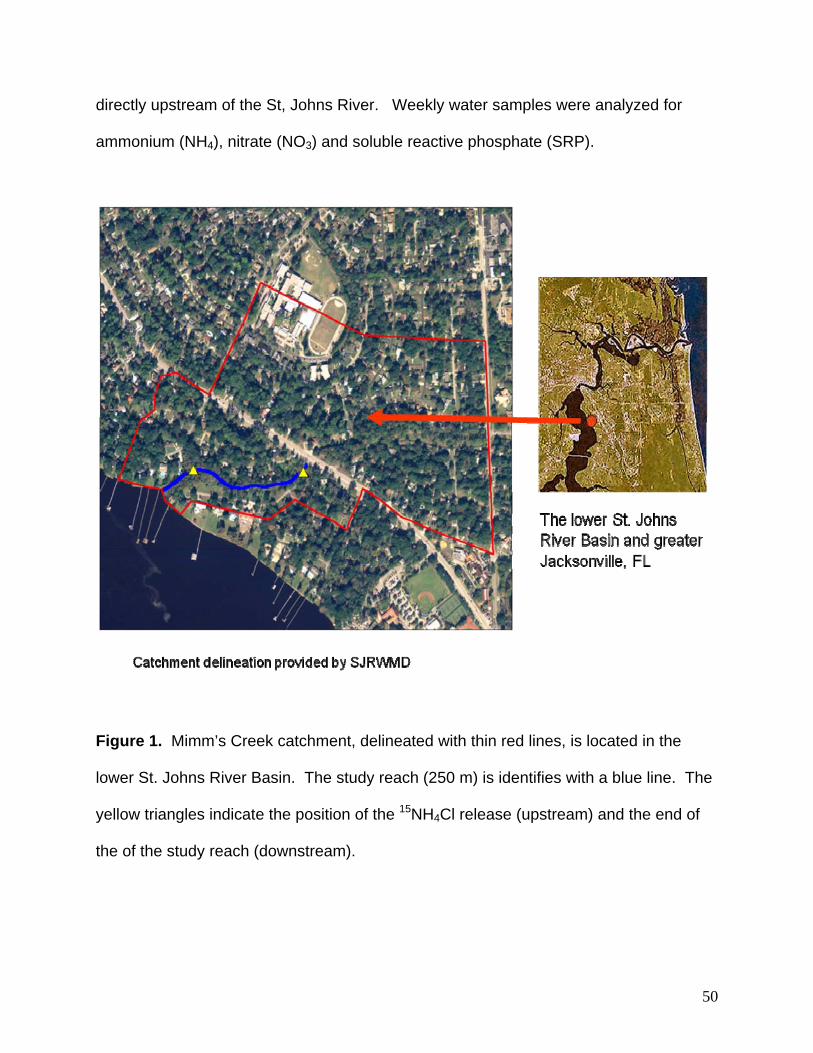
directly upstream of the St, Johns River. Weekly water samples were analyzed for

ammonium (NH4), nitrate (NO3) and soluble reactive phosphate (SRP).

Figure 1. Mimm’s Creek catchment, delineated with thin red lines, is located in the

lower St. Johns River Basin. The study reach (250 m) is identifies with a blue line. The

yellow triangles indicate the position of the 15NH4Cl release (upstream) and the end of

the of the study reach (downstream).

50

Water was filtered on-site and all samples were analyzed within 24 hours of collection.

Water temperatures were measured at the time of collection with a YSI meter. Both the

St. Johns River Water Management District laboratory and contracted laboratories were

used for analysis of the array of water quality constituents. All analyses were performed

using U.S. EPA and Florida Department of Environmental Protection approved methods

(40 CFR 100-149, APHA 1998). Current velocities, water depth, and cross-sectional

area were measured in each stream and used to calculate discharge.

3.2.1 15NH4 uptake experiment

Ammonium uptake was measured in Mimm’s Creek in summer 2006 using stable

isotopes as tracers (see Mulholland et al 2000 for detailed methods). Briefly, we added

15NH4Cl for 21 days (starting on 13 July 2006) using a battery powered fluid metering

pump with the goal to enrich stream 15N by 500‰ without increasing ambient inorganic-

nitrogen concentrations. The solution was added at a constricted portion of the stream

channel to increase mixing. Water samples for 15NH4 were collected one day after the

addition was started (day 1), just before the addition was stopped (day 21), and one day

after the addition was stopped (day 22). Samples were collected from 9 locations (Fig.

2) using a GeopumpTM with an inline filter. Isolation of 15N from the water samples was

accomplished using ammonia diffusion methods (Holmes et al. 1998) and 15N:14N was

quantified by mass spectrometer at the Ecosystem Center laboratory, Marine Biological

Laboratory, Woods Hole, Ma. Uptake length (Sw), uptake velocity (Vf), and whole

stream uptake (U) were then calculated following procedures found in Mulholland et al.

(2000) and Stream Solute Workshop (1990).

51

Figure 2. Locations where water samples were collected along Mimm’s Creek during

the 15NH4Cl tracer experiment.

52


3.3.1 Study site

The catchment of Mimm’s Creek is dominated by urban/residential land use and is

an important conveyance for storm water (Table 1). The 250-meter reach used for the

ammonium addition was deeply incised with sandy substrata. Discharge was uniform

and low (~3 L s-1) and stream NH4 concentrations averaged ~250 μg L-1 during the

release (Table 2).

Table 1. Summary of the distribution of percent land use, percent total impervious area

(PTIA) and catchment area (CA in hectares) for Mimm’s Creek. Residential (LD) is low

density housing with < 2 dwellings per acre, residential (MD) is medium density housing

with 2-5 dwelling per acre, undeveloped land use includes a mixture of wetlands,

forests, ponds, and streams. Impervious area (hectares) was calculated using methods

from Arnold and Gibbons (1996).

========================================================== Land use Area (ha) % cover Impervious area (ha) --------------------------------------------------------------------------------------------------- Residential (LD) 16.6 17 3.3 Residential (MD) 77.4 79 23.2 Commercial 3.9 4 2.9 Undeveloped 0.1 <1 0 ---------------------------------------------------------------------------------------------------

total 98 100 29.4 PTIA 30

==========================================================

53

Table 2. Summary of selected physical and chemical conditions in Mimm’s Creek

during the ammonium uptake experiment started on 13 July 2006.

===================================== Parameter Value

-------------------------------------------------------------- Discharge 3 L s-1 Mean width 1.5 m Mean depth 20 cm

Mean velocity 2.2 cm s-1 Temperature 26 o C NH4 60 – 350 µg L-1 NO3 80 – 850 µg L-1 SRP 90 – 300 µg L-1

=====================================

3.3.2. Ammonium uptake

As expected, δ15N-NH4 declined exponentially with distance from the release

location (Fig. 3A). δ15N-NH4 flux ranged from <0.1 to 0.9 ug 15N s-1 (Fig. 3B). Uptake

lengths (Sw) were 83.6 m and 104.3 m, uptake velocities (Vf) were 0.0315 and 0.0292

mm s-1, and whole stream uptake rates (U) were 0.2295 and 0.3739 g m-2 d-1 on days 1

and 21, respectively.

Ammonium uptake measures for Mimm’s Creek were much different than forest

streams of similar size (e.g., LINX – Webster et al. 2003, Table 3). Uptake length (Sw)

was 3 to 7 times longer, uptake velocity (Vf) were 4 to 9 times slower, and whole stream

uptake (U) was 5 to 10 times greater. Ammonium concentrations in Mimm’s Creek

were also 1 to 2 orders of magnitude greater than the LINX streams. Given this, the

difference we found in uptake are not surprising (sensu Dodds et al. 2002).

54

55

When compared to other urbanized streams in the southeastern United States

(Meyer et al. 2005), values from Mimm’s Creek were similar (Fig. 4). However, these

systems are much larger than Mimm’s Creek which suggest that ambient ammonium

concentration alone (i.e., not stream channel size or flow dynamics) are regulating

uptake rates.

A further comparison of uptake velocities vs. ammonium concentrations among 18

streams of differing size (1st to 3rd order) and land use (forested, urbanized, agriculture,

wastewater effluent) revealed that uptake velocities decreased exponentially (Fig. 5).

From these data it appears that regardless of stream type, ammonium uptake velocities

stabilize at concentrations > 40 µg L-1. When ammonium concentrations are below this

threshold, it is likely that variation in uptake is driven by factors that affect the balance of

autotrophic and heterotrophic metabolism (Dodds et al. 2002, Webster et al. 2003).

When concentrations are above this threshold, uptake velocity are plausibly slowed by

both increased NH4 concentrations and decreased biotic uptake driven by impairment

caused by anthropogenic stressors. (Meyer et al. 2005).

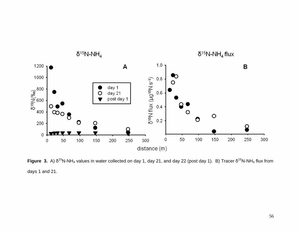
Figure 3. A) δ15N-NH4 values in water collected on day 1, day 21, and day 22 (post day 1). B) Tracer δ15N-NH4 flux from

days 1 and 21.

56

Table 3. Comparison of average ammonium dynamics of Mimm’s Creek with selected

LINX streams (Webster et al. 2003). Uptake length (Sw) is in m, uptake velocity (Vf) is

mm s-1, Total stream uptake (U) is g N m-2 d-1, discharge (Q) is L s-1, ammonium

concentration is µg L-1.

================================================================= Stream Sw Vf U Q NH4 ------------------------------------------------------------------------------------------------------------ Mimm's Creek 94 0.0304 0.3016 3 60-350 Walker Branch 23 0.1360 0.0317 9 3 Bear Brook 14 0.1190 0.0411 4 4 Gallina Creek 21 0.1540 0.0691 6 5 Quebrada Bisley 26 0.1440 0.0523 13 4 Kings Creek 58 0.3020 0.0626 11 2 =================================================================

57

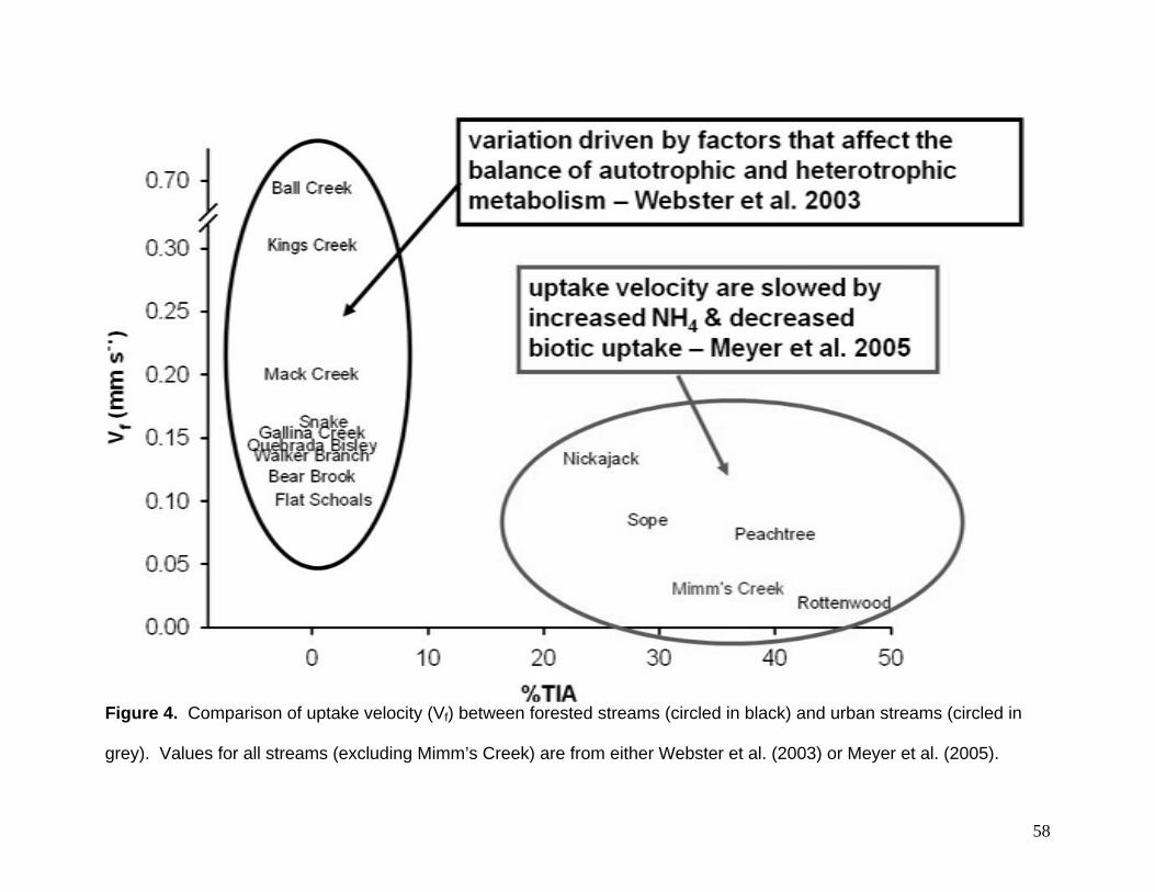
Figure 4. Comparison of uptake velocity (Vf) between forested streams (circled in black) and urban streams (circled in

grey). Values for all streams (excluding Mimm’s Creek) are from either Webster et al. (2003) or Meyer et al. (2005).

58

Figure 5. Comparison of uptake velocities (Vf) vs. ammonium concentrations among 18 streams of differing size and land

use. From these data it appears that regardless of stream type ammonium uptake velocities stabilize at concentrations >

40 µg L-1. WWTP=wastewater treatment plant effluent

59

.

3.4 Conclusion

Understanding how nitrogen dynamics are altered in urbanized headwater streams

is an important step in protecting downstream reaches. This work shows that increased

dissolved nitrogen concentrations due to urbanization result in longer uptake lengths,

slower uptake velocities, but higher whole stream uptake. Further, by comparing our

results with other published values it appears that regardless of land use or stream size,

uptake velocity slows to ~0.03 mm s-1 when ammonium concentrations are greater that

~40 µg L-1. Given this and the degree of development that continues to occur in

greater Jacksonville, eutrophication of the St. Johns River will continue if steps are not

taken to reduce nitrogen loading that originates from lower-order streams.




Arnold, C.L., and C.J. Gibbons. 1996. Impervious surface coverage: the emergence of a

key environmental indicator. Journal of the American Planning Association

62:243-258.

Bernhardt, E.S., and M.A. Palmer. 2007. Restoring streams in an urban context.


Bernot, M.J., J.L. Tank, T.V. Royer and M.B. David. 2006. Nutrient uptake in streams

draining agricultural catchments of the midwestern United States. Freshwater

Biology 51:499–509.

60

Dodds, W. K., A. J. López, W. B. Bowden, S. Gregory, N. B. Grimm, S. K. Hamilton, A.

E. Hershey, E. Martí, W. B. McDowell, J. L. Meyer, D. Morrall, P. J. Mulholland,

B. J. Peterson, J. L. Tank, H. M. Vallet, J. R. Webster and W. Wollheim. 2002.

N uptake as function of concentration in streams. Journal of the North American

Benthological Society, 21, 206–220.

Grimm, N.B., R.W. Sheibley, C. Crenshaw, C.N. Dahm, W.J. Roach and L. Zeglin.

2005. Nutrient retention and transformation in urban streams. Journal of the

North American Benthological Society 24: 626–642

Haggard, B.E., E.H. Stanley and D.E. Storm. 2005. Stream nutrient retention efficiency

in an enriched system. Journal of the North American Benthological Society

24:29-47.

Holmes, R.M., J.W. McClelland, D.M. Sigman, B. Fry and B.J. Peterson. 1998.

Measuring 15N-NH4+ in marine, estuarine and fresh waters: An adaptation of the

ammonia diffusion method for samples with low ammonium concentrations.

Marine Chemistry 60:235-243

Marti, E., J. Autmatell, L. Gode, M. Poch and F. Sabater. 2004. Nutrient retention

efficiency in streams receiving inputs from wastewater treatment plants. Journal

of Environmental Quality 33:285–293.,

Meyer, J. L., M. J. Paul, and W. K. Taulbee. 2005. Stream ecosystem function in

urbanizing landscapes. Journal of the North American Benthological Society

24:602-612.

61

62

Mulholland, P.J., J.L.Tank, D.M. Sanzone, W.M. Wolheim, B.J. Peterson, J.R. Webster,

and J.L. Meyer. 2000. Nitrogen cycling in a forest stream determined by a 15N

tracer addition. Ecological Monographs. 70: 471-493.

Peterson, B.J., W.M. Wollheim, P.J. Mulholland, J.R. Webster, J.L. Meyer, J.L. Tank, E.

Marti, W.B. Bowden, H.M. Valett, A.E. Hershey, W.H. McDowell, W.K. Dodds,

S.K. Hamilton, S. Gregory, and D.J. D’Angelo. 2001. Control of nitrogen export

from watersheds by headwater streams. Science 292:86-90.

Stream Solute Workshop. 1990. Concepts and methods for assessing solute

dynamics in stream ecosystems. Journal of the North American Benthological

Society. 9: 95–119.

Tank, J.L., J.L. Meyer, D. Sanzone, P.J. Mulholland, J.R Webster, B.J Peterson and

Norman E. Leonard. 2000. Analysis of nitrogen cycling in a forest stream during

autumn using a 15N tracer addition. Limnology and Oceanography 45:1013-

1029.

Walsh, C.J., A.H. Roy, J.W. Feminella, P.D. Cottingham, P.M.Groffman and R.P.

Morgan. 2005. The urban stream syndrome: current knowledge and the search

for a cure. Journal of the North American Benthological Society 24:706-723.

Webster, J.R., P.J. Mulholland, J.L. Tank, H.M. Valett, W.K. Dodds, B.J. Peterson, W.B.

Bowden, C.N. Dahm, S. Findlay, S.V. Gregory, N.B. Grimm, S.K. Hamilton, S.L.

Johnson, E. Marti, W.H. McDowell, J.L. Meyer, D.D. Morrall, S.A. Thomas, and

W.M. Wollheim. 2003. Factors affecting ammonium uptake in streams – an

inter-biome perspective. Freshwater Biology 48: 1329-1352.

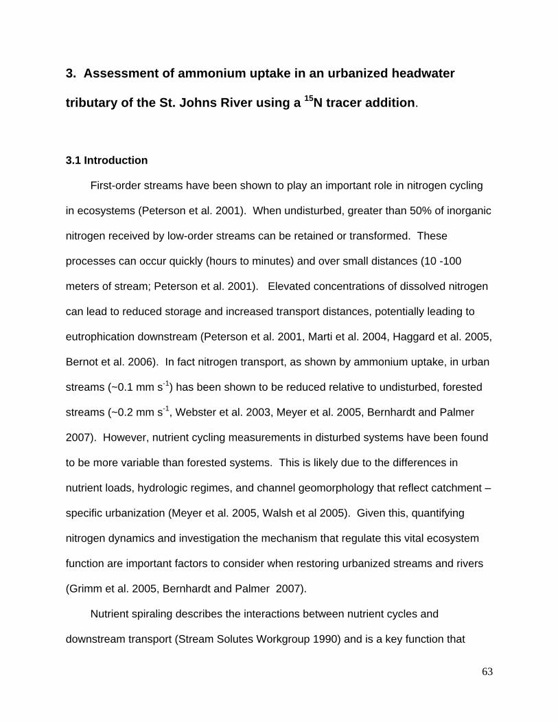
3. Assessment of ammonium uptake in an urbanized headwater

tributary of the St. Johns River using a 15N tracer addition.

3.1 Introduction

First-order streams have been shown to play an important role in nitrogen cycling

in ecosystems (Peterson et al. 2001). When undisturbed, greater than 50% of inorganic

nitrogen received by low-order streams can be retained or transformed. These

processes can occur quickly (hours to minutes) and over small distances (10 -100

meters of stream; Peterson et al. 2001). Elevated concentrations of dissolved nitrogen

can lead to reduced storage and increased transport distances, potentially leading to

eutrophication downstream (Peterson et al. 2001, Marti et al. 2004, Haggard et al. 2005,

Bernot et al. 2006). In fact nitrogen transport, as shown by ammonium uptake, in urban

streams (~0.1 mm s-1) has been shown to be reduced relative to undisturbed, forested

streams (~0.2 mm s-1, Webster et al. 2003, Meyer et al. 2005, Bernhardt and Palmer

2007). However, nutrient cycling measurements in disturbed systems have been found

to be more variable than forested systems. This is likely due to the differences in

nutrient loads, hydrologic regimes, and channel geomorphology that reflect catchment –

specific urbanization (Meyer et al. 2005, Walsh et al 2005). Given this, quantifying

nitrogen dynamics and investigation the mechanism that regulate this vital ecosystem

function are important factors to consider when restoring urbanized streams and rivers

(Grimm et al. 2005, Bernhardt and Palmer 2007).

Nutrient spiraling describes the interactions between nutrient cycles and

downstream transport (Stream Solutes Workgroup 1990) and is a key function that

63

regulates ecosystem structure and function. Nutrient uptake and its inverse, spiraling

length, can be measured with tracer additions (e.g., stable isotope 15N) or short-term

nutrient additions (Stream Solute Workshop 1990, Mulholland et al. 2002, Webster et al.

2003). Both methods have advantages and disadvantages (e.g.., expense vs.

accuracy). Measurements using nutrient additions will tend to overestimate uptake

length and this overestimation is related to both nutrient limitation and concentration of

the addition. Measurements using tracers avoid this problem, but can be much more

expensive. In urbanized streams where nutrients levels can be very high, measuring

nutrient uptake with short-term additions may not feasible due to potential saturation of

biological uptake which necessitates using the tracer methods.

Studies using stable isotopes as tracers have revealed much about nitrogen

dynamics in streams (Mulholland et al. 2000, Tank et al. 2000, Dodds et al. 2002,

Webster et al. 2003, Grimm et al. 2005). However, the majority of these studies have

focused on systems with limited anthropogenic disturbance (however see Grimm et al.

2005). In summer 2006, we conducted a 21-day tracer addition of 15NH4Cl in Mimm’s

Creek, a first-order urban stream in Jacksonville, Florida. Our goal was to investigate

how catchment urbanization affects ammonium uptake.

3.2 Methods

3.2.1 Study site

Mimm’s Creek is a first-order urban stream in Jacksonville, Florida (Fig. 1).

Catchment boundaries and estimates of land cover were provided by the St. John’s

River Water Management District (Fig. 2, Table 1). The study reach (250 m) was

64

directly upstream of the St, Johns River. Weekly water samples were analyzed for

ammonium (NH4), nitrate (NO3) and soluble reactive phosphate (SRP).

Figure 1. Mimm’s Creek catchment, delineated with thin red lines, is located in the

lower St. Johns River Basin. The study reach (250 m) is identifies with a blue line. The

yellow triangles indicate the position of the 15NH4Cl release (upstream) and the end of

the of the study reach (downstream).

65

Water was filtered on-site and all samples were analyzed within 24 hours of collection.

Water temperatures were measured at the time of collection with a YSI meter. Both the

St. Johns River Water Management District laboratory and contracted laboratories were

used for analysis of the array of water quality constituents. All analyses were performed

using U.S. EPA and Florida Department of Environmental Protection approved methods

(40 CFR 100-149, APHA 1998). Current velocities, water depth, and cross-sectional

area were measured in each stream and used to calculate discharge.

3.2.1 15NH4 uptake experiment

Ammonium uptake was measured in Mimm’s Creek in summer 2006 using stable

isotopes as tracers (see Mulholland et al 2000 for detailed methods). Briefly, we added

15NH4Cl for 21 days (starting on 13 July 2006) using a battery powered fluid metering

pump with the goal to enrich stream 15N by 500‰ without increasing ambient inorganic-

nitrogen concentrations. The solution was added at a constricted portion of the stream

channel to increase mixing. Water samples for 15NH4 were collected one day after the

addition was started (day 1), just before the addition was stopped (day 21), and one day

after the addition was stopped (day 22). Samples were collected from 9 locations (Fig.

2) using a GeopumpTM with an inline filter. Isolation of 15N from the water samples was

accomplished using ammonia diffusion methods (Holmes et al. 1998) and 15N:14N was

quantified by mass spectrometer at the Ecosystem Center laboratory, Marine Biological

Laboratory, Woods Hole, Ma. Uptake length (Sw), uptake velocity (Vf), and whole

stream uptake (U) were then calculated following procedures found in Mulholland et al.

(2000) and Stream Solute Workshop (1990).

66

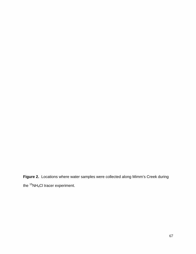
Figure 2. Locations where water samples were collected along Mimm’s Creek during

the 15NH4Cl tracer experiment.

67


3.3.1 Study site

The catchment of Mimm’s Creek is dominated by urban/residential land use and is

an important conveyance for storm water (Table 1). The 250-meter reach used for the

ammonium addition was deeply incised with sandy substrata. Discharge was uniform

and low (~3 L s-1) and stream NH4 concentrations averaged ~250 μg L-1 during the

release (Table 2).

Table 1. Summary of the distribution of percent land use, percent total impervious area

(PTIA) and catchment area (CA in hectares) for Mimm’s Creek. Residential (LD) is low

density housing with < 2 dwellings per acre, residential (MD) is medium density housing

with 2-5 dwelling per acre, undeveloped land use includes a mixture of wetlands,

forests, ponds, and streams. Impervious area (hectares) was calculated using methods

from Arnold and Gibbons (1996).

========================================================== Land use Area (ha) % cover Impervious area (ha) --------------------------------------------------------------------------------------------------- Residential (LD) 16.6 17 3.3 Residential (MD) 77.4 79 23.2 Commercial 3.9 4 2.9 Undeveloped 0.1 <1 0 ---------------------------------------------------------------------------------------------------

total 98 100 29.4 PTIA 30

==========================================================

68

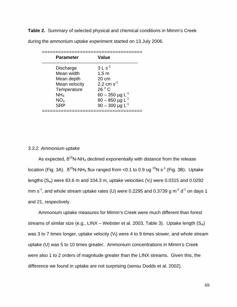
Table 2. Summary of selected physical and chemical conditions in Mimm’s Creek

during the ammonium uptake experiment started on 13 July 2006.

===================================== Parameter Value

-------------------------------------------------------------- Discharge 3 L s-1 Mean width 1.5 m Mean depth 20 cm

Mean velocity 2.2 cm s-1 Temperature 26 o C NH4 60 – 350 µg L-1 NO3 80 – 850 µg L-1 SRP 90 – 300 µg L-1

=====================================

3.3.2. Ammonium uptake

As expected, δ15N-NH4 declined exponentially with distance from the release

location (Fig. 3A). δ15N-NH4 flux ranged from <0.1 to 0.9 ug 15N s-1 (Fig. 3B). Uptake

lengths (Sw) were 83.6 m and 104.3 m, uptake velocities (Vf) were 0.0315 and 0.0292

mm s-1, and whole stream uptake rates (U) were 0.2295 and 0.3739 g m-2 d-1 on days 1

and 21, respectively.

Ammonium uptake measures for Mimm’s Creek were much different than forest

streams of similar size (e.g., LINX – Webster et al. 2003, Table 3). Uptake length (Sw)

was 3 to 7 times longer, uptake velocity (Vf) were 4 to 9 times slower, and whole stream

uptake (U) was 5 to 10 times greater. Ammonium concentrations in Mimm’s Creek

were also 1 to 2 orders of magnitude greater than the LINX streams. Given this, the

difference we found in uptake are not surprising (sensu Dodds et al. 2002).

69

70

When compared to other urbanized streams in the southeastern United States

(Meyer et al. 2005), values from Mimm’s Creek were similar (Fig. 4). However, these

systems are much larger than Mimm’s Creek which suggest that ambient ammonium

concentration alone (i.e., not stream channel size or flow dynamics) are regulating

uptake rates.

A further comparison of uptake velocities vs. ammonium concentrations among 18

streams of differing size (1st to 3rd order) and land use (forested, urbanized, agriculture,

wastewater effluent) revealed that uptake velocities decreased exponentially (Fig. 5).

From these data it appears that regardless of stream type, ammonium uptake velocities

stabilize at concentrations > 40 µg L-1. When ammonium concentrations are below this

threshold, it is likely that variation in uptake is driven by factors that affect the balance of

autotrophic and heterotrophic metabolism (Dodds et al. 2002, Webster et al. 2003).

When concentrations are above this threshold, uptake velocity are plausibly slowed by

both increased NH4 concentrations and decreased biotic uptake driven by impairment

caused by anthropogenic stressors. (Meyer et al. 2005).

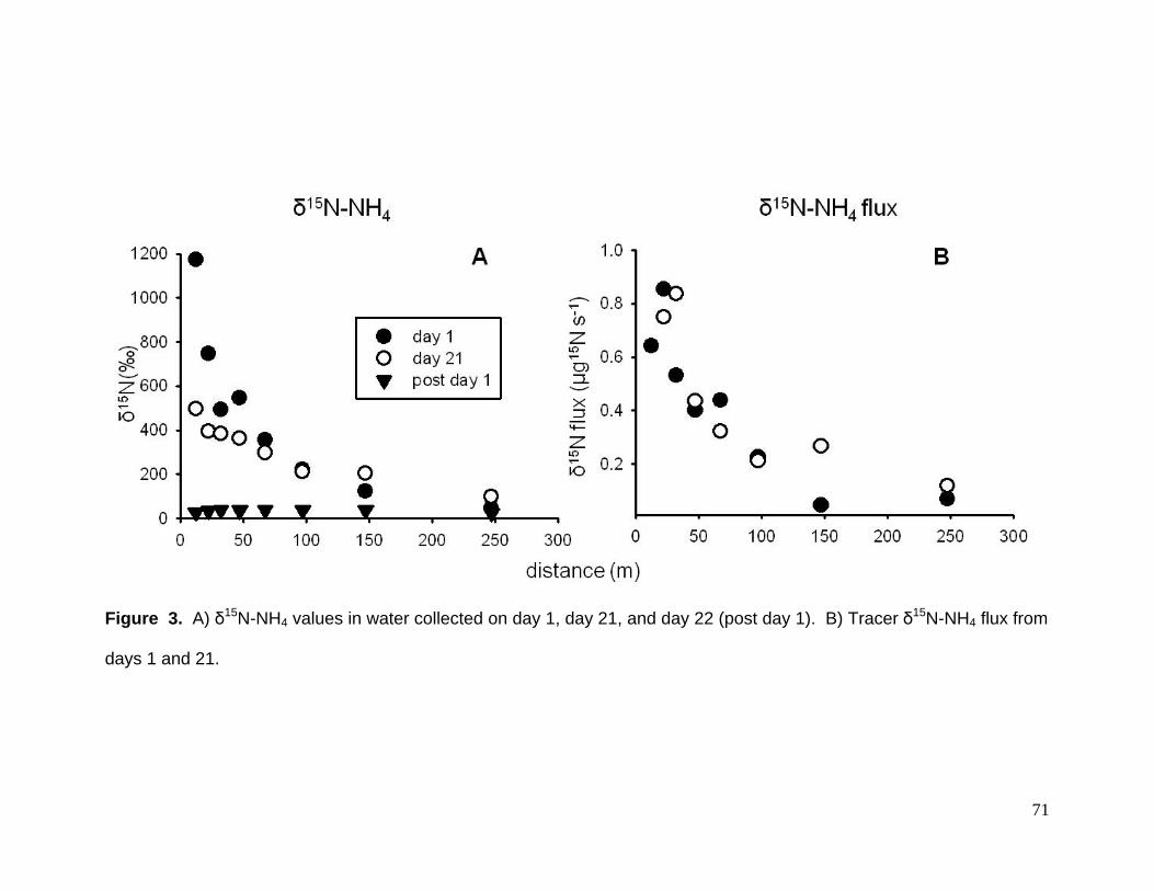
Figure 3. A) δ15N-NH4 values in water collected on day 1, day 21, and day 22 (post day 1). B) Tracer δ15N-NH4 flux from

days 1 and 21.

71

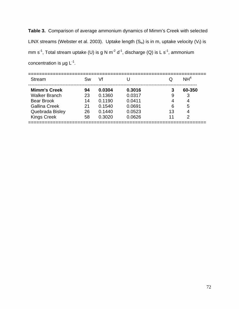
Table 3. Comparison of average ammonium dynamics of Mimm’s Creek with selected

LINX streams (Webster et al. 2003). Uptake length (Sw) is in m, uptake velocity (Vf) is

mm s-1, Total stream uptake (U) is g N m-2 d-1, discharge (Q) is L s-1, ammonium

concentration is µg L-1.

================================================================= Stream Sw Vf U Q NH4 ------------------------------------------------------------------------------------------------------------ Mimm's Creek 94 0.0304 0.3016 3 60-350 Walker Branch 23 0.1360 0.0317 9 3 Bear Brook 14 0.1190 0.0411 4 4 Gallina Creek 21 0.1540 0.0691 6 5 Quebrada Bisley 26 0.1440 0.0523 13 4 Kings Creek 58 0.3020 0.0626 11 2 =================================================================

72

Figure 4. Comparison of uptake velocity (Vf) between forested streams (circled in black) and urban streams (circled in

grey). Values for all streams (excluding Mimm’s Creek) are from either Webster et al. (2003) or Meyer et al. (2005).

73

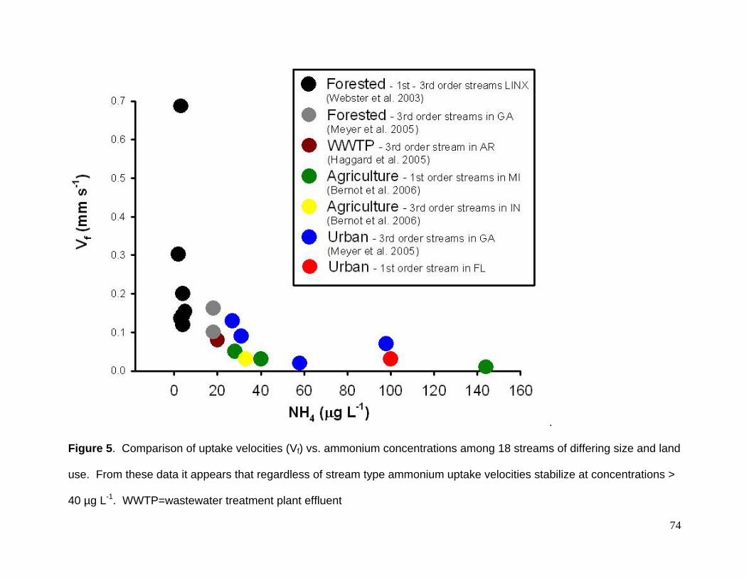
74

Figure 5. Comparison of uptake velocities (Vf) vs. ammonium concentrations among 18 streams of differing size and land

use. From these data it appears that regardless of stream type ammonium uptake velocities stabilize at concentrations >

40 µg L-1. WWTP=wastewater treatment plant effluent

.

3.4 Conclusion

Understanding how nitrogen dynamics are altered in urbanized headwater streams

is an important step in protecting downstream reaches. This work shows that increased

dissolved nitrogen concentrations due to urbanization result in longer uptake lengths,

slower uptake velocities, but higher whole stream uptake. Further, by comparing our

results with other published values it appears that regardless of land use or stream size,

uptake velocity slows to ~0.03 mm s-1 when ammonium concentrations are greater that

~40 µg L-1. Given this and the degree of development that continues to occur in

greater Jacksonville, eutrophication of the St. Johns River will continue if steps are not

taken to reduce nitrogen loading that originates from lower-order streams.




Arnold, C.L., and C.J. Gibbons. 1996. Impervious surface coverage: the emergence of a

key environmental indicator. Journal of the American Planning Association

62:243-258.

Bernhardt, E.S., and M.A. Palmer. 2007. Restoring streams in an urban context.


Bernot, M.J., J.L. Tank, T.V. Royer and M.B. David. 2006. Nutrient uptake in streams

draining agricultural catchments of the midwestern United States. Freshwater

Biology 51:499–509.

75

Dodds, W. K., A. J. López, W. B. Bowden, S. Gregory, N. B. Grimm, S. K. Hamilton, A.

E. Hershey, E. Martí, W. B. McDowell, J. L. Meyer, D. Morrall, P. J. Mulholland,

B. J. Peterson, J. L. Tank, H. M. Vallet, J. R. Webster and W. Wollheim. 2002.

N uptake as function of concentration in streams. Journal of the North American

Benthological Society, 21, 206–220.

Grimm, N.B., R.W. Sheibley, C. Crenshaw, C.N. Dahm, W.J. Roach and L. Zeglin.

2005. Nutrient retention and transformation in urban streams. Journal of the

North American Benthological Society 24: 626–642

Haggard, B.E., E.H. Stanley and D.E. Storm. 2005. Stream nutrient retention efficiency

in an enriched system. Journal of the North American Benthological Society

24:29-47.

Holmes, R.M., J.W. McClelland, D.M. Sigman, B. Fry and B.J. Peterson. 1998.

Measuring 15N-NH4+ in marine, estuarine and fresh waters: An adaptation of the

ammonia diffusion method for samples with low ammonium concentrations.

Marine Chemistry 60:235-243

Marti, E., J. Autmatell, L. Gode, M. Poch and F. Sabater. 2004. Nutrient retention

efficiency in streams receiving inputs from wastewater treatment plants. Journal

of Environmental Quality 33:285–293.,

Meyer, J. L., M. J. Paul, and W. K. Taulbee. 2005. Stream ecosystem function in

urbanizing landscapes. Journal of the North American Benthological Society

24:602-612.

76

77

Mulholland, P.J., J.L.Tank, D.M. Sanzone, W.M. Wolheim, B.J. Peterson, J.R. Webster,

and J.L. Meyer. 2000. Nitrogen cycling in a forest stream determined by a 15N

tracer addition. Ecological Monographs. 70: 471-493.

Peterson, B.J., W.M. Wollheim, P.J. Mulholland, J.R. Webster, J.L. Meyer, J.L. Tank, E.

Marti, W.B. Bowden, H.M. Valett, A.E. Hershey, W.H. McDowell, W.K. Dodds,

S.K. Hamilton, S. Gregory, and D.J. D’Angelo. 2001. Control of nitrogen export

from watersheds by headwater streams. Science 292:86-90.

Stream Solute Workshop. 1990. Concepts and methods for assessing solute

dynamics in stream ecosystems. Journal of the North American Benthological

Society. 9: 95–119.

Tank, J.L., J.L. Meyer, D. Sanzone, P.J. Mulholland, J.R Webster, B.J Peterson and

Norman E. Leonard. 2000. Analysis of nitrogen cycling in a forest stream during

autumn using a 15N tracer addition. Limnology and Oceanography 45:1013-

1029.

Walsh, C.J., A.H. Roy, J.W. Feminella, P.D. Cottingham, P.M.Groffman and R.P.

Morgan. 2005. The urban stream syndrome: current knowledge and the search

for a cure. Journal of the North American Benthological Society 24:706-723.

Webster, J.R., P.J. Mulholland, J.L. Tank, H.M. Valett, W.K. Dodds, B.J. Peterson, W.B.

Bowden, C.N. Dahm, S. Findlay, S.V. Gregory, N.B. Grimm, S.K. Hamilton, S.L.

Johnson, E. Marti, W.H. McDowell, J.L. Meyer, D.D. Morrall, S.A. Thomas, and

W.M. Wollheim. 2003. Factors affecting ammonium uptake in streams – an

inter-biome perspective. Freshwater Biology 48: 1329-1352.

Documents

ASSESSMENT OF THE EFFECTS OF LAND USE CHANGES ON …