Embed Size (px)
Citation preview

Assessment of spatial representation of Groundwater monitoring and
meteorological data in Gaza Strip
By
Ali Abdelkader A. Salha
Supervised By Dr. Fahid Rabah
Dr. Said Ghabayen
A Thesis Submitted in Partial Fulfillment of the Requirements for the Degree of Master of Science in Engineering- Water Resources Engineering
May 2010
The Islamic University of Gaza Deanery of High Studies Faculty of Engineering
Department of Civil Engineering Water Resources Engineering
الجامعة الإسلامية بغزة
عمادة الدراسات العليا
آلية الهندسة
قسم الهندسة المدنية
برنامج هندسة مصادر المياه

ABSTRACT
i
ABSTRACT The Groundwater aquifer in Gaza Strip (semi-arid region) is considered to be the sole source of water exploitation that is extensively deteriorated and may take long time to restore its fresh water conditions. For protecting the groundwater quality and quantity, understanding the data on spatial and temporal distribution of water quality, groundwater level, and rainfall (the only source of natural recharge) are very important. Geostatistics methods are one of the most advanced techniques for interpolation of groundwater related parameters. Accordingly, perceptive spatial variation in groundwater and climate representation is a key decision to many water resource management specialists. However, the most common sources of groundwater and climatic data in Gaza Strip are the domestic water wells including some of the monitoring wells and the meteorological/rainfall stations respectively. This study examines some of the statistical approaches for interpolating both groundwater parameters represented by chloride concentration "and water level and climatic data represented by rainfall rates over Gaza Strip. It also provides a brief introduction to the applicable interpolation techniques for groundwater & climate variables for use in Water resources studies and in addition, draws recommendations for future research to assess interpolation techniques. Basically, one of the problems which often arise in any hydrogeological studies is to estimate data at a given site because either the data are missing or the site is un-gauged or not accessible as Gaza Strip case. Such estimates can be made by spatial interpolation of data available at other sites. A number of spatial interpolation techniques are available today with varying degrees of complexity. In this study, different interpolation methods (IDW, Kriging, and Spline) were applied for predicting the spatial distribution of water quality and rainfall data generated for more than 170 domestic and monitoring water wells as well as 12 rainfall stations. Statistical investigations through normalization of data, modeling of semivariogram, examining powers, tuning smoothing factors were conducted. RMSE and/or R2 were used to select the best fitted model for each interpolation method, and then cross-validation of the best fitted models was using two independent sets of data (modeling data and calibration data). The best method for interpolation was selected based on the lowest RMSE and the highest R2. Results showed that for interpolation of groundwater quality and water level, Kriging method is superior to IDW & Spline methods. In addition to that, the study recommended using Kriging method for the interpolation of the annual rainfall spatial variability unlike what is practiced locally. Finally, using the best fitted interpolation methods and GIS tools, prediction maps of groundwater parameters and rainfall data were prepared.
Keywords: GIS, Interpolation, spatial distribution models, groundwater quality, groundwater level, rainfall, Gaza Strip

ملخـــص الدراســــة
ii
ملخـــص الدراســــة
سية ) المنطقة شبه القاحلة (خزان المياه الجوفي في قطاع غزة يعتبر شرب لاستهلاك أحد المصادر الرئي اه ال ذو هو ومية ةمتدهورنوعية اه العذب ة المي تعادة حال ة . والذي قد يستغرق وقتا طويلا لاس اه الجوفي ة المي ة من حيث ال (و لحماي نوعي
سوبمآو اهلل ن ة وآ) مي ار المناخي ات الأمط ة (مي اه العذب صدر المي ات )م إن البيان ات ف اني والمعلوم ع المك ن التوزي عة ف ولذلك . أهمية خاصة عتبر ذو ت ذه المعايير والزماني له ي ه) Geostatistics(إن الإحصائيات الجيولوجي من ة واحد ل
ة بلمعلومات وال وتمثيلا أآثر التقنيات تطورا لاستخراج ات المكاني ة ليان اه الجوفي ة (لمي سوب آنوعي اه ومن ات لو) المي كمية ار المناخي اين .الأمط إن إدراك التب الي ف عوبالت اني والتوزي ة ول المك سوبلنوعي اخي من ل المن ة والتمثي اه الجوفي المي
مات فإن مصدر المعلو وللعلم. المائية والمصادر رئيسي لقرار آثير من المتخصصين في إدارة الموارد أمرللأمطار هو ة ومحطات الأرصاد الآبار أتي من يالمشترك للمياه الجوفية والبيانات المناخية في قطاع غزة ار المراقب ك آب بما في ذل
.الجوية
ة تفحص الدراسةهذه اه الجوفي اه ( بعض الأساليب الإحصائية لاستخراج آلا من معلومات المي سوب المي ور ومن و) الكلة ات المناخي ار"البيان ك فا يف" الأمط ن ذل ضلا ع زة ، ف اع غ ة قط تخراج لدراس ات الاس وجزة لتقني ة م وفر مقدم ت
)Interpolation methods ( دمت ذلك ق ة ، وآ للمياه الجوفية والمتغيرات المناخية للاستخدام في بحوث الموارد المائي . في المستقبلبعض التوصيات لتقييم تقنيات وطرق المقارنة والتمثيل والتقييم ليتم استخدامها الدراسة
ا قيم هو تقدير هيدروجيولوجيةتنشأ في أي دراسات المشاآل التي غالبا ماأحد ين، إم ات اللأن البيانات في موقع مع بيان
ديرات . قطاع غزة آما فيلا يمكن الوصول إليها مناطق هناك أو لا توجد به أدوات قياسالموقع أن مفقودة أو ذه التق وهتيفاء ن طريقةيتم معرفتها عيمكن أن اني الاس ات المتاحة ) Interpolation Spatial(المك ع و المقاسة للبيان في مواقوم مع .أخرى د هناك عدد من تقنيات الاستيفاء المكانية المتاحة الي ة من التعقي ذه .درجات متفاوت ، يوجد الدراسة في ه
ات اني للبيان ل مك ة تمثي ن طريق ر م ـ أآث ؤ )IDW ، Kriging ،Spline(آ ذآورة للتنب تخدام الطرق الم م اس ث ت ، حية ال آبار من 170بالتوزيع المكاني للبيانات لأآثر من ار المراقب ى آب ة 12و بلديات بالإضافة إل . محطة لللأرصاد الجوي
ة أدوات تصحيح بعد فحص وفرز وتقييم البيانات ، واستخدام ادلات ،)semivariogram(النمذجة التجريبي ديل مع وتعسلاسة معيار الدقة و القوة الي ومعاملات ال ى وبالت اء عل اره بن م اختي د ت دل ق إن أفضل نموذج مع م ف أ ت ة للخط ل قيم أق
سابها ك احت د ذل تخدامه بع تخراج واس ة اس ل طريق ين . لك يم ب ة والتقي ر المقارن م عب ك ث طح اتل تخدام الأس ة باس لمكانيأ ) ت للمعايرةلنمذجة و بيانالبيانات ( للبيانات تينمجموعتين مستقل دار الجذر التربيعي للخط ى وبالاستدلال عن مق واعل
.أفضل طريقة للتمثيل قد تم اختيارف، ها بقيمة ارتباط بين القيم المقاسة والقيم التي تم التنبؤ
فضل هي أ Krigingفإن استخدام طريقة مكانيا ومنسوبهاأن لتمثيل بيانات نوعية المياه الجوفية الدراسة أظهرت نتائج ن ى أن . Spline و IDWم ةبالإضافة إل تخدام الدراس ات هطول Kriging أوصت باس اني لكمي ر المك ل التغي لتمثي
ل أخيراً، وباستخدام طرق. دث في قطاع غزة على عكس ما يحالأمطار السنوي ساعدة نظم التمثي ا وبم م اختياره ي ت التة لتمثيل المكاني لمعلومات المياه الجوفية المعلومات الجغرافية، فقد تم إعداد الخرائط الخاصة با و ومنسوب المياه الجوفي
. الأمطار
نظم المعلومات الجغرافية ، الاستخراج ، نماذج التوزيع المكاني ، نوعية المياه الجوفية ، : الكلمات الأساسية .مستوى المياه الجوفية ، هطول الأمطار ، قطاع غزة

DEDICATIONS
iii
DEDICATIONS
To my sincere father and my sincere mother for their unbounded kindness,
To my wife for her support and encouragement,
To my lovely son (Abdelkader) and lovely daughter (Batol),
To all of my brothers and sisters,
and to my friends and colleagues.

ACKNOWLEDGMENT
iv
ACKNOWLEDGMENT
Thanks to Allah the most compassionate the most merciful for giving me persistence and potency to accomplish this study.
I would like to express my gratitude to my supervisors Dr. Fahid Rabah
and Dr. Said Ghabayen for their guidance and endless support throughout this study. Their encouraging, valuable feedback and combined experiences and insight that have greatly influenced and impacted this study.
I would like to thank the Coastal Municipalities Water Utility (CMWU)
for its generous support and amazing provided data & tools and all my colleagues in particular to Eng. Ashraf Mushtaha and the directors at CMWU for the wonderful working environment I had.
Deep thanks to the Palestinian Water Authority (PWA) for providing its assistance and support.
Last but not least, I would like to thank all those who have assisted,
guided and supported me in my quests leading to this study.
TABLE OF CONTENTS
v
TABLE OF CONTENTS ABSTRACT....................................................................................................................................... I
الدراســــة ملخـــص ................................................................................................................................. II
DEDICATIONS ............................................................................................................................. III
ACKNOWLEDGMENT ............................................................................................................... IV
TABLE OF CONTENTS.................................................................................................................V
LIST OF TABLES ......................................................................................................................... IX
LIST OF FIGURES ....................................................................................................................... XI
LIST OF ABBREVIATIONS AND ACRONYMS .................................................................. XIII
CHAPTER (1): INTRODUCTION ...............................................................................................15 1.1 Background..........................................................................................................................................15 1.2 Statement of the problem....................................................................................................................16 1.3 Study Objectives ..................................................................................................................................17 1.4 Study Methodology..............................................................................................................................17
1.4.1 Mobilization and Data collection phase;........................................................................................17 1.4.2 Data Evaluation and Preparation phase; ........................................................................................18 1.4.3 Spatial Analyst based GIS application and Output Modeling; ......................................................18 1.4.4 Model investigation and verification; ............................................................................................18 1.4.5 Review of applied different interpolations; ...................................................................................18 1.4.6 Final Results review and demonstration; .......................................................................................18
1.5 Study Layout........................................................................................................................................19
CHAPTER (2): STUDY AREA .....................................................................................................21 2.1 Introduction .........................................................................................................................................21 2.2 Location................................................................................................................................................21 2.3 Population ............................................................................................................................................21 2.4 Climate .................................................................................................................................................22 2.5 Gaza Coastal Aquifer ..........................................................................................................................23 2.6 GS Groundwater Characteristics.......................................................................................................25
2.6.1 Quantity .........................................................................................................................................25 2.6.2 Quality ...........................................................................................................................................26 2.6.3 Water Level ...................................................................................................................................27 2.6.4 Meteorological Data / Rainfall ......................................................................................................29
CHAPTER (3): LITERATURE REVIEW ...................................................................................31 3.1 Introduction .........................................................................................................................................31 3.2 GIS Applications in Water Management ..........................................................................................32 3.3 GIS Interpolation Techniques ............................................................................................................34
3.3.1 Trend Surface ................................................................................................................................36 3.3.2 Inverse Distance Weighted ............................................................................................................37 3.3.3 Triangulation .................................................................................................................................39 3.3.4 Spline (Regularized & Tension): ...................................................................................................39

TABLE OF CONTENTS
vi
3.3.5 Kriging...........................................................................................................................................40 2.3.6 Theissen Polygons .........................................................................................................................41
3.4 Model Evaluation & Validation .........................................................................................................42 3.4.1 Accuracy & Model performance Testing.......................................................................................42 3.4.3 Cross validation .............................................................................................................................43
3.5 Software processing.............................................................................................................................44 3.5.1 ArcMap..........................................................................................................................................44 3.5.2 ArcView.........................................................................................................................................45
3.6 Recommended interpolation methods in the study...........................................................................45
CHAPTER (4): METHOD AND MATERIALS ..........................................................................50 4.1 Data employed .....................................................................................................................................50
4.1.1 Groundwater Quality (Chloride - Cl- in mg/l) ...............................................................................50 4.1.2 Groundwater water level (WL in meters) ......................................................................................52 4.1.3 Meteorological data (Rainfall in mm)............................................................................................54 4.1.4 ArcGIS documents.........................................................................................................................54
4.2 Dataset Processing ...............................................................................................................................54 4.2.1 Groundwater Quality (Chloride (Cl-) in mg/l) ...............................................................................55 4.2.2 Groundwater water level (WL in meters) ......................................................................................56 4.2.3 Meteorological data (Rainfall in mm)............................................................................................58
4.3 Methods ................................................................................................................................................59 4.3.1 Applied Interpolation Techniques..................................................................................................59
4.3.1.1 Spline (RBF)...........................................................................................................................59 4.3.1.2 IDW ........................................................................................................................................59 4.3.1.3 Kriging ...................................................................................................................................60
4.3.2 Model Validation & Evaluation.....................................................................................................60 4.3.2.1 Validation...............................................................................................................................60 4.3.2.2 Cross-validation.....................................................................................................................60 4.3.2.3 Evaluation ..............................................................................................................................60
CHAPTER (5): RESULTS & DISCUSSIONS .............................................................................63 5.1 Introduction .........................................................................................................................................63 5.2 Interpolation Application....................................................................................................................63 5.3 Results ..................................................................................................................................................64
5.3.1Chloride Dataset Results.................................................................................................................64 5.3.1.1 2001 dataset ...........................................................................................................................64 5.3.1.2 2003 dataset ...........................................................................................................................67 5.3.1.3 2005 dataset ...........................................................................................................................70 5.3.1.4 2007 dataset ...........................................................................................................................73
5.3.2 Water Level Dataset Results..........................................................................................................77 5.3.2.1 2001 dataset ...........................................................................................................................77 5.3.2.2 2003 dataset ...........................................................................................................................80 5.3.2.3 2005 dataset ...........................................................................................................................83 5.3.2.4 2007 dataset ...........................................................................................................................85
5.3.3 Rainfall Dataset Results.................................................................................................................88 2.3.3.1 2001 dataset ...........................................................................................................................88 5.3.3.2 2003 dataset ...........................................................................................................................90 5.3.3.3 2005 dataset ...........................................................................................................................93 5.3.3.4 2007 dataset ...........................................................................................................................95
5.4 Discussion & Interpretation ...............................................................................................................97 5.4.1 Chloride Dataset Discussion..........................................................................................................98 5.4.2 Water Level Dataset Discussion ....................................................................................................99 5.4.3 Rainfall Dataset Discussion .........................................................................................................100

TABLE OF CONTENTS
vii
5.5 Surface Mapping ...............................................................................................................................101 5.6 Optimized Interpolation Method .....................................................................................................108
5.6.1 Chloride Dataset 2007 .................................................................................................................108 5.6.2 Water Level Dataset 2007............................................................................................................110
CHAPTER (6): CONCLUSIONS AND RECOMMENDATIONS ..........................................113 6.1 Conclusions ........................................................................................................................................113 6.2 Recommendation ...............................................................................................................................114
REFERENCES..............................................................................................................................116
APPENDIXES ...............................................................................................................................123 Appendix 1 – Study Wells' Data.............................................................................................................124 Appendix 2 – Chloride Dataset...............................................................................................................127
Appendix 2.1 - Chloride Dataset in 2001 .............................................................................................127 Appendix 2.2 - Chloride Dataset in 2003 .............................................................................................129 Appendix 2.3 - Chloride Dataset in 2005 .............................................................................................131 Appendix 2.4 - Chloride Dataset in 2007 .............................................................................................134
Appendix 3 – Water Level Dataset ........................................................................................................137 Appendix 3.1 – Water Level Dataset in 2001.......................................................................................137 Appendix 3.2 – Water Level Dataset in 2003.......................................................................................140 Appendix 3.3 – Water Level Dataset in 2005.......................................................................................143 Appendix 3.4 – Water Level Dataset in 2007.......................................................................................146
Appendix 4 – Rainfall Dataset ................................................................................................................149 Appendix 4.1 – Rainfall Dataset in 2000/01.........................................................................................149 Appendix 4.2 – Rainfall Dataset in 2002/03.........................................................................................149 Appendix 4.3 – Rainfall Dataset in 2004/05.........................................................................................150 Appendix 4.4 – Rainfall Dataset in 2006/07.........................................................................................150
Appendix 5 – Chloride Modeling Dataset .............................................................................................151 Appendix 5.1 - Chloride Modeling Dataset in 2001.............................................................................151 Appendix 5.2 - Chloride Modeling Dataset in 2003.............................................................................153 Appendix 5.3 - Chloride Modeling Dataset in 2005.............................................................................155 Appendix 5.4 - Chloride Modeling Dataset in 2007.............................................................................157
Appendix 6 – Water Level Modeling Dataset .......................................................................................160 Appendix 6.1 – Water Level Modeling Dataset in 2001 ......................................................................160 Appendix 6.2 – Water Level Modeling Dataset in 2003 ......................................................................163 Appendix 6.3 – Water Level Modeling Dataset in 2005 ......................................................................166 Appendix 6.4 – Water Level Modeling Dataset in 2007 ......................................................................169
Appendix 7 – Rainfall Modeling Dataset...............................................................................................172 Appendix 7.1 – Rainfall Modeling Dataset in 2001 .............................................................................172 Appendix 7.2 – Rainfall Modeling Dataset in 2003 .............................................................................172 Appendix 7.3 – Rainfall Modeling Dataset in 2005 .............................................................................173 Appendix 7.4 – Rainfall Modeling Dataset in 2007 .............................................................................173
Appendix 8 – Chloride Dataset Histogram & Normalization for years 2001, 2003, 2005, & 2007...174 Appendix 9 – Rainfall Dataset Histogram & Normalization for years 2001, 2003, 2005, & 2007 ....178 Appendix 10 – Kriging Interpolation Method and its Techniques......................................................182 Appendix 11 Validation and Modeling for Chloride............................................................................186
Appendix 11.1 Validation Trials and Results for Chloride in year 2001..............................................186 Appendix 11.2 Validation Trials and Results for Chloride in year 2003..............................................187 Appendix 11.3 Validation Trials and Results for Chloride in year 2005..............................................188 Appendix 11.4 Validation Trials and Results for Chloride in year 2007..............................................189

TABLE OF CONTENTS
viii
Appendix 12 Validation and Modeling for Water Level......................................................................190 Appendix 12.1 Validation Trials and Results for Water Level in year 2001........................................190 Appendix 12.2 Validation Trials and Results for Water Level in year 2003........................................191 Appendix 12.3 Validation Trials and Results for Water Level in year 2005........................................192 Appendix 12.4 Validation Trials and Results for Water Level in year 2007........................................193
Appendix 13 Validation and Modeling for Rainfall .............................................................................194 Appendix 13.1 Validation Trials and Results for Rainfall in year 2001...............................................194 Appendix 13.2 Validation Trials and Results for Rainfall in year 2003...............................................195 Appendix 13.3 Validation Trials and Results for Rainfall in year 2005...............................................196 Appendix 13.4 Validation Trials and Results for Rainfall in year 2007...............................................197

LIST OF TABLES
ix
LIST OF TABLES
Table 4-1. Summary of Chloride dataset in year 2001 .....................................................................50 Table 4-2. Summary of Chloride dataset in year 2003 .....................................................................51 Table 4-3. Summary of Chloride dataset in year 2005 .....................................................................51 Table 4-4. Summary of Chloride dataset in year 2007 .....................................................................52 Table 4-5. Number of wells used for Water level study dataset ..........................................................53 Table 4-6. Rainfall dataset in study years (mm/year) .......................................................................54 Table 4-7. Statistics analysis of Chloride Dataset...........................................................................55 Table 4-8. Statistics analysis of Water Level Dataset .......................................................................56 Table 4-9. Statistics analysis of Rainfall Dataset ............................................................................58 Table 5-1. Calibration dataset of Chloride dataset for year 2001 .......................................................64 Table 5-2. Summary of Validation results for Chloride in year 2001..................................................65 Table 5-3. Predicted values vs. measured Chloride values for year 2001.............................................66 Table 5-4. Summary of Cross Validation values for Chloride in year 2001 .........................................66 Table 5-5. Calibration dataset of Chloride dataset in for year 2003....................................................67 Table 5-6. Summary of Validation results for Chloride in year 2003..................................................67 Table 5-7. Predicted values vs. measured Chloride values for year 2003.............................................69 Table 5-8. Summary of Cross Validation results for Chloride in year 2003 .........................................69 Table 5-9. Calibration dataset of Chloride dataset for year 2005 .......................................................70 Table 5-10. Summary of Validation results for Chloride in year 2005 ................................................71 Table 5-11. Predicted values vs. measured Chloride values for year 2005 ...........................................71 Table 5-12. Summary of Cross Validation results for Chloride in year 2005 .......................................73 Table 5-13. Calibration data of Chloride dataset for year 2007 .........................................................74 Table 5-14. Summary of Validation results for Chloride in year 2007 ................................................74 Table 5-15. Predicted values vs. measured Chloride values for year 2007 ...........................................75 Table 5-16. Summary of Cross Validation results for Chloride in year 2007 .......................................76 Table 5-17. Calibration dataset of Water Level dataset for year 2001 .................................................77 Table 5-18. Summary of Validation results for Water Level in year 2001 ...........................................77 Table 5-19. Predicted values vs. measured Water Level values for year 2001.......................................78 Table 5-20. Summary of Cross Validation results for Water Level in year 2001...................................78 Table 5-21. Calibration dataset of Water Level dataset for year 2003 .................................................80 Table 5-22. Summary of Validation results for Water Level in year 2003 ...........................................80 Table 5-23. Predicted values vs. measured Water Level values for year 2003.......................................81 Table 5-24. Summary of Cross Validation results for Water Level in year 2003...................................81 Table 5-25. Calibration dataset of Water Level dataset for year 2005 .................................................83 Table 5-26. Summary of Validation results for Water Level in year 2005 ...........................................83 Table 5-27. Predicted values vs. measured Water Level values for year 2005......................................83 Table 5-28. Summary of Cross Validation results for Water Level in year 2005...................................84 Table 5-29. Calibration data of Water Level dataset for year 2007.....................................................86 Table 5-30. Summary of Validation results for Water Level in year 2007 ...........................................86 Table 5-31. Predicted values vs. measured Water Level values for year 2007.......................................87 Table 5-32. Summary of Cross Validation results for Water Level in year 2007...................................87 Table 5-33. Calibration dataset of Rainfall dataset for year 2001 ......................................................88 Table 5-34. Summary of Validation results for Rainfall in year 2001.................................................89 Table 5-35. Predicted values vs. measured Rainfall values for year 2001 ............................................90 Table 5-36. Summary of Cross Validation results for Rainfall in year 2001 ........................................90

LIST OF TABLES
x
Table 5-37. Calibration dataset of Rainfall dataset in mm for year 2003.............................................91 Table 5-38. Summary of Validation results for Rainfall in year 2003.................................................91 Table 5-39. Predicted values vs. measured Rainfall values for year 2003 ............................................92 Table 5-40. Summary of Cross Validation results for Rainfall in year 2003 ........................................92 Table 5-41. Calibration dataset of Rainfall dataset for year 2005 ......................................................93 Table 5-42. Summary of Validation results for Rainfall in year 2005.................................................93 Table 5-43. Predicted values vs. measured Rainfall values for year 2005 ............................................94 Table 5-44. Summary of Cross Validation results for Rainfall in year 2005 ........................................95 Table 5-45. Calibration dataset of Rainfall dataset for year 2007 ......................................................95 Table 5-46. Summary of Validation results for Rainfall in year 2007.................................................96 Table 5-47. Predicted values vs. measured Rainfall values in mm for year 2007 ..................................97 Table 5-48. Summary of Cross Validation results for Rainfall in year 2007 ........................................97 Table 5-49. Summary of statistical errors for for Chloride Datasets...................................................98 Table 5-50. Summary of statistical errors for Water Level Datasets ...................................................99 Table 5-51.Summary of statistical errors for Rainfall Datasets ....................................................... 100 Table 5-52. Summary of Statistical errors for Kriging Method for Chloride subsets in year 2007 ......... 108 Table 5-53. Summary of Statistical errors for IDW Method for Chloride subsets in Year 2007............. 108 Table 5-54. Summary of Statistical errors for Kriging method for Water Level datasets in Year 2007 ... 110 Table 5-55. Summary of Statistical errors for IDW method for Water Level subsets in Year 2007 ........ 111

LIST OF FIGURES
xi
LIST OF FIGURES
Figure 1-1. Disposition of the study .............................................................................................19 Figure 2-1. National Geographic location of GS (Courtesy of Wikipedia)...........................................21 Figure 2-2. Projected population in the GS 1997 – 2025. (PCBS, 2007) .............................................22 Figure 2-3. Location of Gaza Coastal Aquifer in Palestine (MEDA, 2007) .........................................23 Figure 2-4. Schematic Drawing of Gaza Aquifer HydroGeologic Cross Section (CMWU, 2008) ............24 Figure 2-5. Section profile details sub-aquifers of the coastal aquifer (Baalousha, 2003)......................24 Figure 2-6. Spatial Chloride concentration in GS for the year 2007 (CMWU, 2008) ............................26 Figure 2-7. Chloride concentration in 2008 for municipal wells in GS...............................................27 Figure 2-8. Spatial Water Level Elevation in GS for year 2007 (CMWU, 2008) ...................................28 Figure 2-9. Water Level Elevation for Municipal Wells in GS for year 2007 .......................................29 Figure 2-10. Location of rain gauging stations within in GS (Hallaq, 2008) .......................................30 Figure 3-1. Several layers used in GIS application in GS by PWA (Obaid, 2007).................................34 Figure 3-2. Different applied Geostatistical application in GIS (ESRI, 2009a) ....................................36 Figure 3-3. Spatial representation with Trend Surface method .........................................................37 Figure 3-4. Spatial representation with IDW method (Bolstad, 2002) ................................................38 Figure 3-5. Spatial representation with Spline method (Bolstad, 2002) ..............................................40 Figure 3-6. Spatial representation with Thiessen Polygons method (Bolstad, 2002)..............................42 Figure 3-7. ArcMap window and related features. ..........................................................................44 Figure 4-1. Wells Distribution in Gaza Strip's Governorate in year 2001............................................51 Figure 4-2. Wells Distribution in Gaza Strip's Governorate in year 2003............................................51 Figure 4-3. Wells Distribution in Gaza Strip's Governorate in year 2005............................................52 Figure 4-4. Wells Distribution in Gaza Strip's Governorate in year 2007............................................52 Figure 4-5. Histogram Graph for Water Level in year 2001 .............................................................56 Figure 4-6. Histogram Graph for Water Level in year 2003 .............................................................57 Figure 4-7. Histogram Graph for Water Level in year 2005 .............................................................57 Figure 4-8. Histogram Graph for Water Level in year 2007 .............................................................58 Figure 4-9. Study flowchart in selection the best interpolation method...............................................62 Figure 5-1. Prediction error statistics Vs Measured for Chloride in Year 2001 resulted from: (a) Kriging, (b) Spline (RBF), and (c) IDW interpolation methods .....................................................................65 Figure 5-2. Correlation Analysis for Chloride in Year 2001 .............................................................66 Figure 5-3. Prediction error statistics for Chloride in Year 2003 resulted from: (a) Kriging, (b) Spline (RBF), and (c) IDW interpolation methods ...................................................................................68 Figure 5-4. Correlation Analysis for Chloride in Year 2003 .............................................................70 Figure 5-5. Prediction error statistics for Chloride in Year 2005 resulted from: (a) Kriging, (b) Spline (RBF), and (c) IDW interpolation methods ...................................................................................72 Figure 5-6. Correlation Analysis for Chloride in Year 2005 .............................................................73 Figure 5-7. Prediction error statistics for Chloride in Year 2007 resulted from: (a) Kriging, (b) Spline (RBF), and (c) IDW interpolation methods ...................................................................................75 Figure 5-8. Correlation Analysis for Chloride in Year 2007 .............................................................76 Figure 5-9. Prediction error statistics for Water level in Year 2001 resulted from: (a) Kriging, (b) Spline (RBF), and (c) IDW interpolation methods ...................................................................................79 Figure 5-10.Correlation Analysis for Water Level in Year 2001........................................................79 Figure 5-11. Prediction error statistics for Water level in Year 2003 resulted from: (a) Kriging, (b) Spline (RBF), and (c) IDW interpolation methods ...................................................................................82 Figure 5-12.Correlation Analysis for Water Level in Year 2003........................................................82

LIST OF FIGURES
xii
Figure 5-13. Prediction error statistics for Water level in Year 2005 resulted from: (a) Kriging, (b) Spline (RBF), and (c) IDW interpolation methods ...................................................................................85 Figure 5-14. Correlation Analysis for Water Level in Year 2005 .......................................................85 Figure 5-15. Prediction error statistics for Water level in Year 2007 resulted from: (a) Kriging, (b) Spline (RBF), and (c) IDW interpolation methods ...................................................................................87 Figure 5-16. Correlation Analysis for Water Level in Year 2007 .......................................................88 Figure 5-17. Prediction error statistics for Rainfall in Year 2001 resulted from: (a) Kriging, (b) Spline (RBF), and (c) IDW interpolation methods ...................................................................................89 Figure 5-18. Correlation Analysis for Rainfall in Year 2001 ............................................................90 Figure 5-19. Prediction error statistics for Rainfall in Year 2003 resulted from: (a) Kriging, (b) Spline (RBF), and (c) IDW interpolation methods ...................................................................................92 Figure 5-20.Correlation Analysis for Rainfall in Year 2003 .............................................................93 Figure 5-21. Prediction error statistics for Rainfall in Year 2005 resulted from: (a) Kriging, (b) Spline (RBF), and (c) IDW interpolation methods ...................................................................................94 Figure 5-22. Correlation Analysis for Rainfall in Year 2005 ............................................................95 Figure 5-23. Prediction error statistics for Rainfall in Year 2007 resulted from: (a) Kriging, (b) Spline (RBF), and (c) IDW interpolation methods ....................................................................................96 Figure 5-24. Correlation Analysis for Rainfall in Year 2007 ............................................................97 Figure 5-25. R2 vs. number of modeled samples in IDW method for Chloride subsets in Year 2007 ...... 109 Figure 5-26. R2 vs. number of modeled samples in Kriging method for Chloride subset in Year 2007 ... 109 Figure 5-27. Performance of Kriging and IDW for modeled Chloride subsets in Year 2007 ................ 110 Figure 5-28. R2 vs. number of modeled samples in IDW method for Water Level subset in Year 2007 ... 111 Figure 5-29. R2 vs. number of modeled samples in Kriging method for Chloride subsets in Year 2007 .. 112 Figure 5-30. Performance of Kriging and IDW for modeled Water Level subsets in Year 2007 ............ 112

LIST OF ABBREVIATIONS AND ACRONYMS
xiii
LIST OF ABBREVIATIONS AND ACRONYMS
CAMP : Coastal Aquifer Management Program Cl : Chloride CMWU : Coastal Municipalities Water Utility Co : Degrees Celsius DEM : Digital elevation models EC : Electrical conductivity EQA : Environment Quality Authority ESRI : Environmental Systems Research Institute FAO : Food & Agriculture Organization GIS : Geographic Information System GS : Gaza strip ha : 10.000 m2 IAMP : Integrated Aquifer Management Plan IDW : Inverse distance weighted km2 : Square kilometers m/d : meter per day m2/d : square meters per day m3/d : Cubic meter per day m3/yr : cubic meters per year MCM : Million Cubic Meters ME : Mean error mg/L : Milligram Per Liter Mm : millimeters MoA : Ministry of Agriculture MoH : Ministry of Health MOPIC : Ministry of Planning and International Cooperation MSL : mean sea level OK : Ordinary Kriging PCBS : Palestinian Central Bureau of Statistics PHG : Palestinian Hydrology Group ppm : Part Per Million PWA : Palestinian Water Authority RBF : Radial Basis Functions RMSE : Root Mean Squared Error SAR : Sodium Adsorption Ratio TDS : Total Dissolved Solid TH : Total hardness TIN : Triangulated irregular networks UNRWA : United Nations Welfare Relief Agency USAID : U.S. Agency for International Development UV : Ultra Violet

LIST OF ABBREVIATIONS AND ACRONYMS
xiv
WHO : World Health Organization WL : Water Level

CHAPTER (1): INTRODUCTION
15
CHAPTER (1): INTRODUCTION
1.1 Background Water is a precious, finite, and scarce resource in our region, and competition for water from industrial and domestic users continues to grow. No resource is more crucial than water, and no resource in Gaza Strip (GS) is surrounded by more controversy. Basically, groundwater "Coastal Aquifer" is the only source of fresh water in the Gaza Strip. Municipal groundwater wells are currently being used for drinking and domestic purposes while private wells are being used for irrigation not to mention the increasing number of household water wells. The GS is one of the most densely populated areas in the world population of 1,480,000 inhabitants (PCBS, 2007) More than 90% of the population is connected to the municipal drinking water network while the other 10%, mainly rural or distant areas is dependent on the private wells. Generally, GS is a semi arid area with an average annual rainfall ranging between 200-mm/ year in the southern part of the area and 400-mm/ year in the north. Ground water is the only source of water in GS, and many estimation of the annual groundwater recharge in the GS have been mentioned in different references. Although different values for this recharge are given, all of these references agree on one fact, that the annual recharge is less than the abstracted quantities for along time, resulting in a serious mining of the groundwater resources and a net deficit of about 30-40 Million cubic meters (MCM)/year. (CMWU, 2008) In GS the only resource of water for domestic, industry and agriculture use is groundwater. Surface water is not considered as a source of water because Wadi Gaza has the run-off only in winter season and the Israelis turned the direction before it reaches the Palestinian boarder. There are an estimated 4000 wells within the GS. Almost all of these are privately owned and used for agricultural purposes. (PWA, 2000b). Throughout the water studies implemented in GS at the beginning of 1994 and during the implementation of different management programs at especially via the Palestinian Water Authority (PWA) (in particular, Integrated Aquifer Management Plan study (IAMP) and related master plan studies in water and wastewater section, several software systems were used in for modeling, simulating, monitoring, and mapping different characteristics of Gaza aquifer parameters along with the meteorological data over the Gaza strip. The success of these management programs and studies was primarily reliant on the quality and the quantity of data obtained and the associated monitoring system (data collection system). Monitoring system in GS consists of monitoring wells and networks that were established to characterize Gaza coastal aquifer on a quantitatively and qualitatively respects. The establishment of monitoring system was mainly prolonged during the IAMP study and Coastal Aquifer Management Program

CHAPTER (1): INTRODUCTION
16
(CAMP) implementation plan, as many wells were rehabilitated and utilized for monitoring issues (IAMP, 2000). Currently, there are more than 140 wells (domestic) are now used in fresh groundwater abstraction, monitoring and data fetching, but before, that figure reached 600 wells (domestic and agricultural) in early of 2000 but due to many financial, technical, and political matters, the monitoring system was finally based on some of the above municipal wells and monitoring wells with total of 103 Wells (CMWU, 2009). The obtained data from these domestic and monitoring wells were used in mapping the characteristics of Gaza groundwater subjected to water quality, water levels, groundwater flow, and recharge zones…etc to be used in formulating the strategic plans and required project needed for groundwater sustainability. The mapping output had been conducted by using Geographic Information System (GIS) based packages using ArcGIS ArcMap software. Wise management, development, protection, and allocation of water resources is based on sound data regarding the location, quantity, quality, and use of water and how these characteristics are changing over time. The quantity and quality of available water varies over space and time, and is influenced by multifaceted natural and man-made factors including climate, hydrogeology, management practices, pollution…etc. As the foundation for water-resources decision-making, sound data must be continuous over space and time. (PWA, 2000a). GIS applications were first used locally in the beginning of 1995 in different ministries for different purposes (planning, land use, urbanization, road networks …etc) but it was intensively utilized in 1997, in a study funded by the USAID titled as (IAMP), implemented through PWA and other institution with concern, where mapping the groundwater and demonstrating its characteristics was one of the core outputs of that study and a keystone for further groundwater prospected projects, spatial interpretation of Gaza Aquifer quality parameters (mainly Chloride and Nitrate), hydrogeological distribution analysis and other related monitoring issues.
1.2 Statement of the problem It is worth mentioning that Groundwater quality mapping over extensive areas is the first step in water resources planning (Todd, 1980). So, data for generating the required mapping surfaces are usually collected through field sampling and surveying of the established collection system (domestic and monitoring wells). After conducting all required analyzing and screening processing, the resulted mapping output and existing situation representation for different groundwater parameters (e.g. chloride, nitrate and water levels) proved on long term of not having an accurate representation for the whole GS due to either lack of available data in some areas, error in the sampling process or false representation of data in some other areas in the GS, yet many issues were behind these representation problems;
1. Uncertainties concerning monitoring wells’ records affect the spatial representation accuracy and efficiency where many locations with no available data.

CHAPTER (1): INTRODUCTION
17
2. High cost and limited resources availability, the data collection can be conducted only in selected point locations with limited numbers e.g. domestic and monitoring wells.
3. To generate a continuous surface of a property (i.e. groundwater table), some kind of interpolation methods have to be used to estimate surface values at those locations where no samples or measurements were taken.
4. To our knowledge, the evaluation of different interpolation methods and performance for higher accuracy has not taken place in any research or study about Gaza Strip.
An important part of groundwater modeling is the accuracy of input data such as hydraulic head and sink or source that should be assigned to each node of the network. On the other hand, in groundwater, due to aspects of time and cost, data monitoring (such as observation wells) is conducted at a limited number of sites. As a result, non-sampled values should be usually interpolated. Statistics based on spatial distribution, which is usually referred to as geostatistics, is a very useful tool for handling spatially distributed data (Kholghi & Hosseini, 2008).
1.3 Study Objectives The main objective of this study is to evaluate the different interpolation method subjected to spatial representation of groundwater data and meteorological data in GS under the current collection monitoring system along with setting up recommendation for the best suited method for GS status. Yet, this study has three primary objectives:
To conduct comparative evaluation of the different interpolation methods and provide some insights on how these methods should be used properly to generate surface mapping for different sets of data under the existing monitoring programme.
To recommend data managing and processing and provide suggestion as how the data set should be prepared and preprocessed prior to surface generation
To optimize the interpolation methods or techniques examined in order to be utilized for accurate surface representation of areas with missing data points under the available data.
1.4 Study Methodology
1.4.1 Mobilization and Data collection phase; Mobilization of the required tools and software needed for study purpose and
objectives. Communication with PWA, CMWU, Ministry of Agriculture (MoA), Ministry
of Health (MoH), Meteo stations and others. Collection and review of all relevant literature, reports, and projects and any
other documents pertaining to the study's objectives. Collection of Gaza Coastal Aquifer data and the historical data of different
groundwater parameters for the last 8 years (i.e. 2000 - 2007). These data are chloride, and water levels along with meteorological rainfall parameter.

CHAPTER (1): INTRODUCTION
18
Introducing the different interpolation methods used for surface mapping and a theoretical comparison is to be made.
Interpreting different sets of data and its quantity-distance relationship to as basis for selection the appropriate interpolation method and to evaluation the distribution of the existing monitoring system.
1.4.2 Data Evaluation and Preparation phase; The collected data shall be evaluated and checked against its accuracy,
recording, location, documentation and historical background. Pre-processing activities such as verifying, modifying, emerging, screening for
the different collected data in order to be used for GIS based application. Data shall be in form of excel (tables), access (queries) office files and based
shape GIS files and themes.
1.4.3 Spatial Analyst based GIS application and Output Modeling; The Major technique used in comparing the different interpolation methods
adequacy and how spatially is speared in based GIS system. Converting different data themes and shape files into grid maps for purpose of
calculations and value mapping output. Setting out the boundaries, different assumptions and margins of model output
accuracy. Spatial Analyst based GIS application for each of selected parameter based on
its data set arrangement and resulted surface mapping output.
1.4.4 Model investigation and verification; The resulted output surface mapping shall be investigated and verified for its
validity and accuracy through comparing the output results with actual measured data from the field in different locations.
Margins of accuracy and errors will be computed as criteria for final decision of recommended interpolation method using the correlation factor criteria.
1.4.5 Review of applied different interpolations; As a result, different interpolation models and mapping output shall be
demonstrated and interpreted in detailed against the proposed following items; o Monitoring data set criteria. o Interpolation method used. o Model accuracy and investigation result. o Comparison tables, and images output.
1.4.6 Final Results review and demonstration; Finally the recommended interpolation method will be summarized describing
factor of validation and obstacles to be overcome by optimizing the maximum correlation factor "R2" and minimization of "RMSE".
Exploring a relationship between the existing monitoring system and the needed spatial representation of different sets of groundwater data.
Recommendation regarding the most applicable interpolation method under the existing monitoring system in GS and prospected improvements in terms of interpolation method, spatial distribution, and sampling issues.

CHAPTER (1): INTRODUCTION
19
1.5 Study Layout The study layout as shown in Fig. 1-1, consists of the introductory work, background information about the status of the GS groundwater, As the problem is identified and stated with respect to the representation of the variables and what its rule in the decision making process under discussed scenarios and various options. The result of such discussions and scenarios are listed, analyzed and based on that conclusion, recommendations were followed with respect to the results. Chapter one presents the introduction about GS aquifer condition and situation with regard to mapping and spatial representation. It also presents the problem definition, study justification, main goal and purposes of this study. Methodology and study outline. Chapter two describes the GS area, its location, population, climate, and hydrology. The Project study area and its parameters were also addressed that will be used for more interpolation techniques exploration and mapping. Chapter three reviews the literature related to the Geostatistics methods in addition to the different interpolation techniques for mapping the groundwater quality parameters and the meteorological data in GS. Chapter four deals with the data sampled and collected, the process applied for dataset processing through screening, scheduling, correction, and finalization to be used later. The related interpolation analysis methods that have been followed in this study were addressed. Also there will be an introduction to the different processes that will be applied in each interpolation method. All related validation, cross validation and model fitting techniques were discussed and highlighted.
Figure 0-1. Disposition of the study Chapter five presented the results and discussion, different interpolation methods (IDW, Kriging, and Spline methods) were applied for predicting the spatial distribution of the above data generated for more than 170 domestic and monitoring water wells & 12 meteorological stations. Statistical investigation through normalization of data, modeling of semivariogram, optimizing powers, and tuning smoothing factors were conducted. The least RMSE value was used to select the best
Chapter 1 Introduction
Chapter 2Study Area
Chapter 3 Literature Review &
Pervious Studies
Chapter 4 Data Management &
Tools
Chapter 5Results and Discussions
Chapter 6 Conclusion &
Recommendation

CHAPTER (1): INTRODUCTION
20
fitted model for each interpolation method and the for next step process. Then cross-validation of the best fitted models was using two independent sets of data (modeling data and calibration data) where the lowest RMSE and the highest R2, the best method for interpolation was selected. Results showed that for interpolation of Groundwater quality and water level Kriging method is superior to IDW & Spline methods. In addition the study recommended using the Kriging interpolation method interpolating annual climate rainfall spatial variability unlike what is practiced locally. Finally, using the best fitted interpolation methods and GIS tools, prediction maps of Groundwater parameters and rainfall data were prepared and compared among each other towards acceptable assessment of the current situation and hence correct decision being made aftermath. Chapter six stated the conclusions and recommendations resulting from the study.

CHAPTER (2): STUDY AREA
21
CHAPTER (2): STUDY AREA
2.1 Introduction The Palestinian territories consist of the West Bank with approximately 5,800 km2 and the GS with about 365 km2. The West Bank area is made up of a hilly region in the West and the Jordan Valley in the East. The climate in the West Bank can be characterized as hot and dry during summer and cool and wet in winter. The GS has a Mediterranean climate and consists mainly of coastal dune sands, being located between the coast and the Negev and Sinai Deserts (MOPIC, 1998)
2.2 Location The Gaza Strip (GS) is located at the south-eastern coast of the Mediterranean Sea as show in Fig. 2-1 below, on the edge of the Sinai Desert between longitudes 34° 2” and 34° 25” east, and latitudes 31° 16” and 31° 45” north. It has an area of about 365 km2 and its longest width is about 45 m. (MOPIC, 1998) The GS is confined between the Mediterranean Sea in the west, Egypt in the south and the 1950 Armistice line drawn by Rhodes Agreement of 1949 between the Arab States and Israel. Until 1948, the GS was part of Palestine under the British Mandate. From 1948 to 1967, it was under Egyptian administration (Qahman, 2003).
Figure 0-1. National Geographic location of GS (Courtesy of Wikipedia)
2.3 Population GS is considered one of the most overpopulated areas all over the world. As it was stated, the area of GS is about 365 square kilometer with a population of 1,480,000

CHAPTER (2): STUDY AREA
22
inhabitants most of them are refugees (PCBS, 2007). According to Palestinian bureau statistics council (PCBS) population growth rate in GS is 3.8 % which means that the available sources in GS are facing high threat. Moreover the unevenly distribution of population makes the problem of sources allocation more complicated. Nowadays, Gaza city is the biggest population centre and has about 496,410 inhabitants. Gaza's other two main population centers are southern area (Khanyounis and Rafah) with population of 270,979, followed by northern area with 270,245 inhabitants (PCBS, 2007). Moreover Fig. 2-2 shows the population projection up to year 2025 in Gaza Strip which will impose a true challenge to PWA/CMWU and other utilities for providing adequate water.
Figure 0-2. Projected population in the GS 1997 – 2025. (PCBS, 2007)
2.4 Climate GS climate is typical Eastern Mediterranean with hot dry summers and mild winters. Temperature gradually changes throughout the year, reaches its maximum in August (summer) and its minimum in January (winter), the average monthly maximum temperature range from about 17.6 C° for January to 29.4 °C for August while the average monthly minimum temperature for January is about 9.6 °C and 22.7 for August. Gaza Northern area has the highest rainfall rate over GS as on average it has 429mm annually. The average daily mean temperature ranges from 25 °C in summer to 13 °C in winter. Average daily maximum temperatures range from 29 °C to 17 °C and minimum temperatures from 21 °C to 9 °C in the summer and winter respectively. The daily relative humidity fluctuates between 65% in the daytime and 85% at night in the summer, and between 60% and 80% respectively in winter. The mean annual solar radiation amounts to 2200 J/cm2/day (Qahman, 2003). The GS is located in the transitional zone between the arid desert climate of the Sinai Peninsula in Egypt and the temperate and semi-humid Mediterranean climate along the coast. This fact could explain the sharp decrease in rainfall quantities of more than

CHAPTER (2): STUDY AREA
23
200 mm/year between Beit-Lahia in the north and Rafah in the South of GS. (Shahen, 2007) The rainfall data of the GS is based on the data collected from 12 rain stations. The average annual rainfall varies from 450 mm/yr in the north to 200 mm/yr in the south of the GS. Most of the rainfall occurs in the period from October to March, the rest of the year being completely dry.
2.5 Gaza Coastal Aquifer The entire GS lies within the Coastal groundwater basin over the Coastal Aquifer. The Coastal Basin covers an area of 2,000 square kilometers as shown in Fig. 2-3, and is located in the Coastal Plain physiographic province. The Coastal Aquifer is comprised of water-bearing sand, sandstone, gravel, and conglomerate that typically overlie relatively impervious clay, marl, limestone, and chalk (EXACT, 1998).
. Figure 0-3. Location of Gaza Coastal Aquifer in Palestine (MEDA, 2007)
The Gaza aquifer is composed of Quaternary deposits that include layer of loess, dune sand, calcareous sandstone, silt, and clay. Clay layers, which begin at the coast and feather out approximately 4 km from the sea, separate the main aquifer into various sub-aquifers near the shore. The base of the aquifer is the low-permeability Saqiya Formation (Tertiary age), and approximately 1 km thick wedge of marine clay, shale, and marl. (Qahman, 2001).

CHAPTER (2): STUDY AREA
24
The thickness of the saturated groundwater aquifer underneath the GS ranges from few meters in the eastern and south east of the GS to about 120- 150m in the west and along the Mediterranean Sea as shown in Figs. 2.4 and 2.5. The aquifer is mainly composed of unconsolidated sand stone known as Kurkar formation, which overlaying the impermissible layer called Saqiya formation which is considered as the bottom of the Gaza Coastal Aquifer with thickness varies from 800-1000m. The thickness of the unsaturated aquifer which is the overlaying part of the saturated groundwater aquifer ranges from 70–80m in the eastern and south-eastern part of the GS to about few meters in the western and along the coast.
Figure 0-4. Schematic Drawing of Gaza Aquifer HydroGeologic Cross Section
(CMWU, 2008)
Figure 0-5. Section profile details sub-aquifers of the coastal aquifer (Baalousha,
2003) Groundwater flows naturally from east to west. In the northern part of Gaza, water levels range from about 2 meters above mean sea level at the eastern border with Israel to mean sea level along the shore. In the southern part, the water level gradient is steeper, from about 10 meters above sea level near the eastern border to mean sea level along the shore. Municipal and agricultural pumping interrupts seaward flow. In

CHAPTER (2): STUDY AREA
25
some places, flow directions have been reversed as a result of over-pumping. The total estimated production pumping in 1996 was about 40 million m3/yr from municipal wells supply and about 80 million m3/yr from agricultural supply (irrigation). Extractions by Israeli settlements have been estimated to approach 10 million m3/yr (Qahman, 2001). The transmissivity values ranges between 700 and 5000 m2/d. Corresponding values of hydraulic conductivity are mostly within a range of 20-80 m/d. Specific yield values are estimated to be about 15-30 % while specific storativity is about 10-4 from tests conducted in GS (Metcalf & Eddy, 2000).
2.6 GS Groundwater Characteristics
2.6.1 Quantity The only source of water in GS is groundwater which is used for domestic, agricultural and agricultural consumption. In 2007 the total production of water in GS was 173 MCM; the domestic consumption was 85 MCM while the remaining 87MCM for the agriculture sector. 97.5 % of this quantities produced by water wells while 2.5% was imported from Israel Company called Mekerot (PCBS, 2007). The coastal aquifer holds approximately 5000×106 m3 of groundwater of different quality. However, only 1400×106 m3 of this is “freshwater”, with Chloride (Cl-) content of less than 500 mg/l. This fresh groundwater typically occurs in the form of lenses that float on the top of the brackish and/or saline groundwater. That means approximately 70% of the aquifer are brackish or saline water and only 30% are fresh water found mainly in the Northern Governorate. The lateral inflow from the GS borders to the aquifer is estimated at between 18 to 30 ×106 m3/y. Some recharge is available from the major surface flow (Wadi Gaza). However, the extraction from Wadi Gaza, in Israel, limits this recharge to 1.5 to 2 ×10⁶ m3. As a result, the total freshwater recharge at present is limited to approximately 56 to 62×106 m3/y (Metcalf & Eddy, 2000). The aquifer is recharged mainly by rainfall and other minor sources such as leakage of water system, irrigation return flow, and wastewater discharge. The average annual rainfall in the GS varies between 500 mm in the north to 200 mm in the south. Thus, the average annual rainfall in the GS based on 20 years average is 320 mm y-1. The total amount of groundwater recharge from rainfall is about 43 million m3 per year (Baalousha, 2005). According to Metcalf and Eddy 2000 study, the irrigation return flow in the GS varies between 20 and 25 million m3. The available groundwater quantity could be identified if the saturated aquifer reservoir thickness is known in addition to the hydrological parameters of the aquifer such as effective porosity. The area of the groundwater reservoir is limited to the area of the political border of the GS. The area where the groundwater quantity less than 250mg/L is about 44.8 km2, and with an effective porosity of 20%, also with a saturated groundwater ranging from 10 to 50m, hence the stored fresh groundwater quantity is ranging from 100MCM to 450MCM. In previous studies in year 2000, the same calculation has been performed where the groundwater quantity was ranging from 450MCM to 600MCM, which led to a depletion of about

CHAPTER (2): STUDY AREA
26
250MCM from freshwater since year 2000. It is observed that the domestic and industrial usage were about 83MCM (CMWU, 2008).
2.6.2 Quality The groundwater quality is monitored through all municipal wells and some agricultural wells distributed all over the GS. The agricultural monitoring wells are tested against chloride and nitrate ions twice a year by the MoA, while the municipal wells are monitored through all the cations and anions twice a year with the cooperation of both MoH and CMWU. The groundwater quality is varies from place to another and from depth to another as presented in Fig. 2-6 below. The chloride ion concentration varies from less than 250mg/l in the sand dune areas as the northern and south-western area of the GS to about more than10,000 mg/l where the seawater intrusion has occurred (CMWU, 2008).
Figure 0-6. Spatial Chloride concentration in GS for the year 2007 (CMWU,
2008) Quality of the groundwater is a major problem in GS. The aquifer is highly vulnerable to pollution. The domestic water is becoming more saline every year and average chloride concentrations of 500 mg/l or more is no longer an exception. The permissible limits for nitrate are exceeded by a factor of eight for a number of public wells. Most of the public water supply wells don’t comply with the drinking water

CHAPTER (2): STUDY AREA
27
quality standards and concentrations of chloride and nitrate of the water exceed the World Health Organization (WHO) standards in most drinking water wells of the area and represent the main problem of groundwater quality. Over pumping of groundwater and salt water intrusion are the main reasons behind high chloride concentration (CAMP, 2000). Figure 2.7, shows the variation of the concentration of chloride parameter in mg/l for the municipal wells operated in Gaza Strip.
Chloride Concentration
0.00
500.00
1,000.00
1,500.00
2,000.00
2,500.00
3,000.00
3,500.00
4,000.00
4,500.00
5,000.00
C_20
C_79A
C_137
A_211
A_180
E_01
E_90
Q_72
D_75
D_70
E_154
R_162
HA
R_162
CA
R_162
DR_1
12R_2
54R_2
93R_7
5
R_25B
R_25D
R_307
R_310
R_309
J_146 J_
3K_2
1T_5
2G_3
0F_
205
F_19
2S_
71S_
72Ma'a
n
Rashwan
_C
L_189
AL_4
3L_8
7L_1
87L_1
79P_1
54P_
159
P_13
9P_1
48Sh
uka
Wells
Chl
orid
e Va
lue
(mg/
L)
Figure 0-7. Chloride concentration in 2008 for municipal wells in GS
Moreover, it is worth mentioning that Groundwater quality in the Gaza aquifer is generally poor. Over-exploitation has resulted in saltwater intrusion and up-coning. In most areas of Gaza, a slow, continuing decline in groundwater levels has been observed since the mid-1970s (Qahman, 2003). Thus, the uncontrolled discharge of untreated sewage to the ground surface and excessive use of fertilizers led to high nitrate levels in certain areas. With the limited rainfall and high evapotranspiration of the GS it may take long time to restore fresh water conditions in the aquifer (EQA, 2004). Which take us to the point that the water quality in Gaza is affected by many different water sources including soil/water interaction in the unsaturated zone due to recharge and return flows, mobilization of deep brines, sea water intrusion or upconing and disposal of domestic and industrial wastes into the aquifer (Ghabayen et al. 2006)
2.6.3 Water Level The groundwater elevation map in Fig. 2-8 below with respect to the mean sea level (MSL) shows two sensitive areas for groundwater depression; the north and the south areas. As the groundwater level elevation drops 3m in the north and more than 12m in the south below mean sea level. This drop in the groundwater will led to lateral
WHO limit 500 mg/l

CHAPTER (2): STUDY AREA
28
invasion of seawater due to pressure difference and direct contact with the aquifer, and also vertical invasion from deep saline water (CMWU, 2008).
Figure 0-8. Spatial Water Level Elevation in GS for year 2007 (CMWU, 2008)
The extraction from coastal aquifer is almost twice the available recharge that has resulted in dropping the water level by 20-30 cm per year (PWA, 2003). In general term, the water level in Gaza Aquifer dropped on average of 1.6 meters per year, but mostly in the south (Rabi, 2008). As quoted, the active wells are shallow wells and typically their screens are 10-20 m below the water table. Of these wells, about 140 agricultural wells and 39 piezometric wells are presently used to monitor the water levels every month. The agriculture wells of about 10 inches diameters are used as water level monitoring wells. The total depth of most of the wells is not defined clearly. Generally, the total penetrated saturated thickness of these wells is ranging between 30 and 40 m. Most of the piezometric wells are located mainly along the coastal zone and range in depth from 20 to 200 m. Many of these wells have screens at different depths. The piezometric wells have deteriorated and many of these wells have been damaged. (Mogheir, 2003). Figure 2.9 shows clearly the drop in water level in meters with respect to MSL considerably in the monitoring and some of the municipal wells for year 2007

CHAPTER (2): STUDY AREA
29
Graph of WL_07
WELL_IDA_31 A_64 C_27 C_61 CAMP_1B CAMP_8 E_32 F_43 G_13 H_5 L_18 L_8 L_94 N_16 P_48A Piezo_22B Piezo_2B Piezo_3A R_133 R_38 S_28 T_26
WL_
07
10
8
6
4
2
0
-2
-4
-6
-8
-10
-12
Figure 0-9. Water Level Elevation for Municipal Wells in GS for year 2007
2.6.4 Meteorological Data / Rainfall Rainfall is a main component for charging and renewal of groundwater resources in the GS. Estimation of rainfall data is necessary in many natural resources and agricultural studies (Chegini, 2001). Rainfall is one of the most important parts of the water resource. It is an essential component of scientific investigation of the hydrologic cycle. The pattern and the amount beside the intensity of rainfall are the most important factors that directly affect to groundwater balance and replenishment (PWA, 2007). Rainfall in GS is the main source of groundwater recharge area. The area is located in the semi-arid zone and there is no source of recharge other than rainfall therefore a detailed knowledge of rainfall regime and its distribution is a perquisite for water resources planning and management in GS. Considering the amount of rainfall quantity is about 110MCM/year, where part of that is feeding the groundwater aquifer through natural recharging process. The recharge rate is varying in accordance to the soil porosity and the thickness of the unsaturated zone that overlaying the groundwater aquifer. Previous studies showed that the recharge rate is about 25% in the low porous area like the eastern part of the GS, and about 75% in porous area where the sand dunes are still found in the north and south of the GS. Also the rainfall intensity plays an important role in the recharge quantity to the aquifer (CMWU, 2008) The long term average recharge is considered to be 40% of the whole rainfall quantity (PWA, 2005).

CHAPTER (2): STUDY AREA
30
In GS there are 12 manual rainfall stations distributed through different governorates as shown in Fig.2-10. Data from these stations are collected on a daily basis, these stations are operated by ministry of agriculture and data obtained from these stations are entered manually in Palestinian water authority database.
Figure 0-10. Location of rain gauging stations within in GS (Hallaq, 2008)
In 2006-2007 season, the average rainfall depth over GS area is estimated about 364.7 mm with total amount 133.1 MCM received through 46 rainy days. Despite of the small area of GS (365km2), the level of rainfall varies significantly from one area to the next with an average seasonal rainfall of 521.9 mm in north area (north governorate), to 225 mm in the southern area (Rafah governorate) (PWA, 2007), Only 60 MCM was infiltrate into the ground aquifer while the total abstracted quantity was 166MCM (PCBS, 2007).

CHAPTER (3): LITERATURE REVIEW
31
CHAPTER (3): LITERATURE REVIEW
3.1 Introduction A Geographical Information System "GIS" is defined as “an organized collection of computer hardware, software, geographic data, and personnel designed to efficiently capture, store, update, manipulate, analyze, and display all forms of geographically referenced information”. GIS technology has been widely used in various fields, such as agriculture, business geographic, ecology, electricity and gas, emergency management and public safety, environmental management, forestry, health care, education, mining and geosciences, real estate, remote sensing, telecommunications, transportation and water distribution and resources (ESRI, 1992). In addition, GIS is a system of hardware, software, data, people, organizations and institutional arrangements for collecting, storing, analyzing and disseminating information about areas of the earth. (Dueker & Kjerne, 1989) Thus, accurate and reliable groundwater resource information is critical to planners and decision-makers at all levels of government, researchers, developers and the business community (Shivraj & Jothimani, 2002). With the advent of Geographical Information Systems (GIS) has added new vistas in the field of ground water resources mapping and management. It helps in the integrating remotely sensed derived data with ancillary data to have more precise and correct information about various factors involved in the ground water resources management. (Toleti & Chaudhary, 2000). The last decade has seen a phenomenal growth in the use of remote sensing and GIS technology in ground water studies as the ground water has become the most sought after natural resources by the mankind due to tremendous pressure on the ground water system by the ever-increasing population and individual growth (Srivastav & Ahmed, 2003). By adopting a GIS platform the result obtained will be faster and more accurate. Till recently, ground water assessment was based on laboratory investigation, but the advent of Satellite Technology and GIS has made it very easy to integrate various databases. Groundwater is a most important natural resource required for drinking, irrigation and industrialization. The resource can be optimally used and sustained only when quantity and quality of groundwater is assessed. It has been observed that lack of standardization of methodology in estimating the groundwater and improper tools for handling the same, leads to miscalculation of estimation of groundwater (Kharad & Rao, 1999) Assessing groundwater parameters and determination of its characteristics on a spatial scale is an essential prerequisite to understand and to mitigate any economical and social impacts. The main coupling aspect of water availability and water use/management is achieved by balancing the water resources available for water use. Thus it is really important to understand the condition and the status of groundwater parameters and to be distinguished.

CHAPTER (3): LITERATURE REVIEW
32
The use of geographic information system (GIS) and remote sensing to facilitate the estimation of hydrologic parameters for watersheds has gained increasing attention in recent years. This is mainly due to the fact that hydrologic models include both spatial and geomorphic variations. GIS technology provides suitable alternatives for efficient management of large and complex databases (Melesse et al, 2002). Several studies have been done to incorporate GIS in hydrologic modeling of watersheds. These studies have different scopes and can be generally grouped into four categories. Computation of input parameters for existing hydrologic models is the most active area in GIS related hydrology (Djokic & Maidment, 1991; Olivera & Maidment, 1999). Hydrologic assessment refers to the mapping and display in GIS of hydrologic factors that pertain to some situation (Ragan & Kossicki, 1991). Measuring the spatial extent of hydrologic variables from paper maps may be tedious, labor-intensive and error prone. Watershed surface mapping refers to the uses of GIS in representation of watershed surface through the use of digital elevation model and girded geographic data (Sasowsky & Gardner, 1991; Smith & Brilly, 1992). The application of any hydrologic model requires efficient management of large spatial data. This is done by integrating watershed simulation models and GIS which generates the capacity to manage large volumes of data in a common spatial structure (Al-Sabhan et al, 2003).
3.2 GIS Applications in Water Management Good quality societal and technical information is a pre-requisite for successful integrated water management (GWP, 2000). Many studies have shown that GIS can play a very important role in water management in aspects that include analysis and presentation of societal and technical information, identifying the root causes of problems and planning activities and interventions aimed at solving these problems (Rama et al, 2003). Theoretically, in GIS applications for water sector, generating surfaces is a frequently imposed requirement in the early stage of analyses. Topographic surfaces, bedrock surfaces, groundwater tables, and contamination plumes are examples of surfaces which need to be generated from available data sources. The importance of generating these surfaces is that these surfaces are used as the basic information to perform further spatial analyses in environmental applications. Based on these surfaces, we can carry out additional analyses to answer questions such as what is the water level here or there, or how the contamination is distributed in subsurface soil. Thus, the accuracy of subsequent analyses directly depends on the accuracy of the surfaces built in the early stage of analyses. GIS applications for the water industry started evolving in the late 1980s. In the early 1990s, the water industry had started to use GIS in mapping, modeling, facilities management, and work-order management for developing capital improvement programs and operations and maintenance plans (Morgan & Polcari, 1991). In the mid-1990s, GIS started to see wide applicability to drinking water studies. Potential applications identified at that time included (Schock & Clement, 1995):

CHAPTER (3): LITERATURE REVIEW
33
GIS can provide the basis for investigating the occurrence of regulated contaminants for estimating the compliance cost or evaluating human health impacts.
Mapping can be used to investigate process changes for a water utility or to determine the effectiveness of some existing treatment such as corrosion control or chlorination.
GIS can assist in assessing the feasibility and impact of system expansion.
GIS can assist in developing wellhead protection plans. GIS technology has eased previously laborious procedures. Exchange of data between GIS, CAD, supervisory control and data acquisition (SCADA), and hydrologic and hydraulic (H&H) models is becoming much simpler. For example, delineating watersheds and stream networks has been simplified and the difficulty of conducting spatial data management and model parameterization reduced (Miller et al., 2004). The GIS assisted database system would help to apply groundwater management practices such as; proper groundwater resource management in terms of groundwater quality & quantity, Integrated management of water, land use and the environment; to optimize pumping rates with respect to the capacity of the aquifer system, and to prevent groundwater quality deterioration through proper monitoring & evaluation (Maruo, 2004). Yet GIS technology has played critical roles in all aspects of watershed management, from assessing watershed conditions through modeling impacts of human activities on water quality and to visualizing impacts of alternative management scenarios (Tim & Mallavaram, 2003). Representation and analysis of water-related phenomena by GIS facilitates their management. GIS applications that are of particular importance to water industry professionals are: mapping, monitoring, modeling, and maintenance (Shamsi, 2005). The GIS has the ability to store, arrange, retrieve, classify, manipulate, analyze and present huge spatial data and information in a simple manner Application of GIS and Remote Sensing Techniques in Identification, Assessment and Development of Groundwater Resources. (Howari et al., 2007). GIS provides a common framework – spatial location – for watershed management data obtained from a variety of sources. Because watershed data and watershed biophysical processes have spatial dimensions, GIS can be a powerful tool for understanding these processes and for managing potential impacts of human activities. The modeling and visualization capabilities of modern GIS, coupled with the explosive growth of the Internet and the World Wide Web, offer fundamentally new tools to understand the processes and dynamics that shape the physical, biological and chemical environment of watersheds. The linkage between GIS, the Internet, and environmental databases is especially helpful in planning studies where information exchange and feedback on a timely basis is very crucial and more so when there are several different agencies and stakeholders involved. (Tim & Mallavaram, 2003). At the highest level of technology, a GIS can provide a spatial database of information to support modeling of phenomena. The GIS supplies the spatial data in a

CHAPTER (3): LITERATURE REVIEW
34
form that can be input to deterministic or statistical models. The spatial power of the GIS database is used in full by the model, and more detailed and spatially averaged results are produced. This represents a high level of integration and achievement that is now seen in the industry. It has taken a while for such applications to develop, however. This is due to the absence of spatially integrated models for water resource phenomena. Many models use spatial data but average or summarize these data by watershed and/or sub-watershed, and thereby lose much of the detail of spatial variability that often influences phenomena. This is the same level of detail necessary to provide high quality model simulations. In general, the strength of GIS is that it is possible to process the data sets using any type of numerical analysis procedure. In particular, certain procedures are valuable for data visualization and analysis, including image processing techniques, virtual reality, and simulation modeling. (Naamani, 2002). As we can finally summarize it as the integrating capabilities of a GIS can provide an interface to translate and emulate the complexities of a real world system within the confines of a digital world accurately and efficiently (Tim & Mallavaram, 2003). In Gaza Strip, new technique about the integration of applications of geographic information systems and Water Information System in the PWA Offices in Gaza Strip and West Bank which have been used to provide information in water resource management, Licenses Management and Technical issues. The contribution of geographic information system is mainly focus on generation, management, and delivery of spatially distributed data, in Gaza Strip. PWA spatial data vision is building of layers for various water related features its input values from oracle database and connected completely with GIS as shown in Fig. 3-1. GIS was useful in Management of large data sets as GIS proved to be efficient in managing large amounts of Water data. (Obaid, 2007).
Figure 0-1. Several layers used in GIS application in GS by PWA (Obaid, 2007)
3.3 GIS Interpolation Techniques Often geographic data are sampled at various locations, rather than a complete census, because of time or money constraints. To create a surface from sampled data, that is

CHAPTER (3): LITERATURE REVIEW
35
to estimate the values at all non-sampled locations, one needs to interpolate. There is a variety of interpolation methods, but all make use of the First Law of Geography, that things closer together tend to be more similar than those farther away (Theobald, 2007). Interpolation is the process by which a surface is created, usually a raster dataset, through the input of data collected at a number of sample points. There are several forms of interpolation, each which treats the data differently, depending on the properties of the data set. In comparing interpolation methods, the first consideration should be whether or not the source data will change (exact or approximate). Interpolation is a justified measurement because of a Spatial Autocorrelation Principle that recognizes that data collected at any position will have a great similarity to, or influence of those locations within its immediate vicinity. Digital elevation models (DEM), triangulated irregular networks (TIN), Edge finding algorithms, Theissen Polygons, Fourier analysis, Weighted moving averages, Inverse Distance Weighted, Moving averages, Kriging, Spline, and Trend surface analysis are all mathematical methods to produce interpolative data (Wikipedia, 2009a). GIS based packages, offers several interpolation methods for creating surfaces. These methods include but not limited to: trend surface (trend), inverse distance weighted (IDW), triangulation, Kriging and others. Each of these methods has its own advantages and disadvantages in terms of data interpolation processing. None of these method works universally as the best for all the data set. Selection of a particular method depends on the distribution of data points and the study objectives (Jun, 2001). Spatial interpolators may be used to estimate values at non-sampled sites. Spatial interpolation can also be used when preparing irregularly scattered data to construct a contour map or contour surface, which is a two-dimensional representation of a three dimensional surface. All spatial interpolation methods investigated accept irregularly scattered data and can create a regular grid of interpolated points amenable to contouring. Methods that produce smooth surfaces include various approaches that may combine regression analyses and distance-based weighted averages. As explained in more detail below, a key difference among these approaches is the criteria used to weight values in relation to distance. Criteria may include simple distance relations (e.g., inverse distance methods), minimization of variance (e.g., Kriging and cokriging), minimization of curvature, and enforcement of smoothness criteria (splining). On the basis of how weights are chosen, methods are “deterministic” or “stochastic.” Stochastic methods use statistical criteria to determine weight factors (Hartkamp et al., 1999). Interpolation methods can also be described as “global” or “local.” Global techniques (e.g. inverse distance weighted averaging; (IDWA) fit a model through the prediction variable over all points in the study area. Typically, global techniques do not accommodate local features well and are most often used for modeling long-range variations. Local techniques, such as splining, estimate values for a non-sampled point from a specific number of neighboring points. Consequently, local anomalies can be accommodated without affecting the value of interpolation at other points on the

CHAPTER (3): LITERATURE REVIEW
36
surface (Burrough, 1986). Splining, for example, can be described as deterministic with a local stochastic component (Burrough & McDonnell, 1998). In ArcGIS Geostatistical Analyst, it provides a variety of interpolation methods for the creation of an optimal interpolated surface from your data. A friendly wizard helps you through the interpolation process. There are two main groupings of interpolation techniques: deterministic and Geostatistical. Deterministic interpolation techniques are used for creating surfaces from measured points based on either the extent of similarity (e.g., Inverse Distance Weighted) or the degree of smoothing (e.g., Radial Basis Functions). Geostatistical interpolation techniques are based on statistics and are used for more advanced prediction surface modeling, which also includes error or uncertainty of predictions (ESRI, 2000). Fig 3.2 below shows different spatial representation through applying different interpolation method.
Figure 0-2. Different applied Geostatistical application in GIS (ESRI, 2009a)
Surface interpolation functions create a continuous (or prediction) surface from sampled point values. There is a variety of ways to derive a prediction for each location; each method is referred to as a model. With each model, there are different assumptions made of the data, and certain models are more applicable for specific data—for example, one model may account for local variation better than another. Each model produces predictions using different calculations (ESRI, 2009a). Main commonly used interpolation methods can be summarized as following;
3.3.1 Trend Surface The linear trend surface interpolator creates a floating-point grid as shown in Fig. 3-3. It uses a polynomial regression to fit a least-squares surface to the input points. It

CHAPTER (3): LITERATURE REVIEW
37
allows the user to control the order of the polynomial used to fit the surface. Trend interpolation is easy to understand by considering a first-order polynomial (Naoum & Tsanis, 2004). The idea behind the trend surface interpolation is to fit a least-squares surface to observational data points by using polynomial regression. The advantage of this method is that it is superficially easy to understand, at least with respect to the way the surfaces are estimated. It can be used to show broad features of the observational data points, such as the overall flow direction of groundwater (Jun, 2001).
Figure 0-3. Spatial representation with Trend Surface method
3.3.2 Inverse Distance Weighted IDWA is a deterministic estimation method whereby values at non-sampled points are determined by a linear combination of values at known sampled points (Hartkamp et al., 1999). In this interpolation method, observational points are weighted during interpolation such that the influence of one point relative to another declines with distance from the new point. Weighting is assigned to observational points through the use of a weighting power that controls how weighting factors drop off as the distance from new point increases. The greater the weighting powers, the less effect points far from the new point have during interpolation. As the power increases, the value of new point approaches the value of the nearest observational point (Jun, 2001). The inverse-distance weighted procedure is versatile, easy to program and understand, and is fairly accurate under a wide range of conditions (Lam, 1983). Using this method, the property at each unknown location for which a solution is sought is given by:

CHAPTER (3): LITERATURE REVIEW
38
Where Pi is the property at location i; Pj is the property at sampled location j; Dij is the distance from i to j; G is the number of sampled locations; and n is the inverse-distance weighting power. The value of n, in effect, controls the region of influence of each of the sampled locations. As n increases, the region of influence decreases until, in the limit, it becomes the area which is closer to point i than to any other. When n is set equal to zero, the method is identical to simply averaging the sampled values. (Watson & Philip, 1985). The interpolation technique used in the analysis is inverse distance weighted (IDW) method. IDW is an algorithm for spatially interpolating, or estimating values between measurements. Each value estimated in an IDW interpolation is a weighted average of the surrounding sample points. Weights are computed by taking the inverse of the distance from an observation’s location to the location of the point being estimated (Burrough & McDonnell, 1998). The IDW method is fast, easy to implement and easily “tailored” for specific needs. The method allows anisotropy in the source data. Ancillary data cannot be incorporated. Measure of success is through cross validation. There is no extrapolation: all interpolated values are within the range of the data points (De Smith et al., 2007). Fig. 3-4 shows the spatial representation of a surface using IDW interpolation.
Figure 0-4. Spatial representation with IDW method (Bolstad, 2002)
)/1
/
1
1
∑
∑
=
== G
j
nij
G
j
niji
i
D
DPP

CHAPTER (3): LITERATURE REVIEW
39
3.3.3 Triangulation Triangulation is the most flexible interpolation method. It can generate interpolated surfaces from many different data sources such as point data, lines, break lines, and polygons (erase, replace, or clip). Because of this flexibility and the speed of interpolation, triangulation has become a popular interpolation method for GIS users (Jun, 2001). There are several triangulation methods available (Watson, 1992). Delaunay triangulation is the method adopted where value for a new node is ensured to be as close as possible to a known observation point, and triangulation is not affected by the order of observational points to be considered. The main disadvantage is that the surfaces are not smooth and may give jagged appearance. This is caused by discontinuous slopes at the triangle edges and data points. In addition, triangulation is generally not suitable for extrapolation beyond the domain of observed data points.
3.3.4 Spline (Regularized & Tension): Spline interpolation consists of the approximation of a function by means of series of polynomials over adjacent intervals with continuous derivatives at the end-point of the intervals. Smoothing Spline interpolation enables to control the variance of the residuals over the data set. The solution is estimated by an iterative process. It is also referred to as the basic minimum curvature technique or thin plate interpolation (Naoum & Tsanis, 2004). There are two Spline methods: Regularized and Tension. The Regularized method creates a smooth, gradually changing surface with values that may lie outside the sample data range. The Tension method controls the stiffness of the surface according to the character of the modeled phenomenon. It creates a less smooth surface with values more closely constrained by the sample data range. Spline technique has been described by (Wahba 1980) and computationally developed by (Hutchinson 1991) for use with climate data principally in mind. The degree of smoothness, or inversely the degree of complexity, of the fitted function is usually determined automatically from the data by minimizing a measure of predictive error of the fitted surface given by the generalized cross validation. Below in Fig. 3-5 shows the spatial representation features and the lines where mapped by using Spline interpolation method.

CHAPTER (3): LITERATURE REVIEW
40
Figure 0-5. Spatial representation with Spline method (Bolstad, 2002)
The Spline method can be thought of as fitting a rubber-sheeted surface through the known points using a mathematical function. In ArcGIS, the Spline interpolation is the Radial Basis Function (RBF). These functions allow analysts to decide between smooth curves or tight straight edges between measured points. Advantages of splining functions are that they can generate sufficiently accurate surfaces from only a few sampled points and they retain small features. A disadvantage is that they may have different minimum and maximum values than the data set and the functions are sensitive to outliers due to the inclusion of the original data values at the sample points (Sharolyn, 2003).
3.3.5 Kriging Kriging is a term coined by G. Matheron in 1963 after the name of D.G. Krige. Kriging is based on a statistical model of a phenomenon instead of an interpolating function. It uses a model for a spatial continuity in the interpolation of unknown values based on values at neighboring points (Sunila et al., 2004). Kriging is a weighted moving averaging method of interpolation. It is derived from regionalized variable theory which assume that the spatial variation of any geological, soil, or hydrological property, known as a ‘regionalized variable’ is statistically homogenous throughout the surface,; that is, the same pattern of variation can be observed at all locations on the surface (Jun, 2001). Kriging provides a means of interpolating values for points not physically sampled using knowledge about the underlying spatial relationships in a data set to do so. Variograms provide this knowledge. Kriging is based on regionalized variable theory which provides an optimal interpolation estimate for a given coordinate location, as well as a variance estimate for the interpolation value. It involves an interactive

CHAPTER (3): LITERATURE REVIEW
41
investigation of the spatial behavior of the phenomenon before generating the output surface. (Burrough, 1986). The general formula for interpolator method is formed as a weighted sum of the data (ESRI, 2009b),
Where: Z(si) = the measured value at the ith location. λi = an unknown weight for the measured value at the ith location. so = the prediction location. N = the number of measured values.
It is based on the regionalized variable theory, which assumes that the spatial variation in the phenomenon is statistically homogeneous throughout the surface; that is, the same pattern of variation can be observed at all locations on the surface. This hypothesis of spatial homogeneity is fundamental to the regionalized variable theory. Data sets known to have spikes or abrupt changes are not appropriate for the Kriging technique. In some cases, the data can be pre-stratified into regions of uniform surface behavior for separate analysis. (Oliver, 1990). The presence of a spatial structure where observations close to each other are more alike than those that are far apart (spatial autocorrelation) is a prerequisite to the application of geostatistics (Robinson & Metternicht, 2006). More information about Kriging interpolation method can be found in Appendix 10.
2.3.6 Theissen Polygons Thiessen polygons, also referred to as the Dirichlet Tessellations or the Voronoi Diagrams, are an exact method of interpolation that assumes that the values of non-sampled locations are equal to the value of the nearest sampled point. This method is commonly used in the analysis of climatic data when the local observations are not available, and so the data from the nearest weather stations are used. Thiessen polygons define the individual 'regions of influence' around each of a set of points such that any location within particular polygon is nearer to that polygon's point than to any other point, and therefore, has the same value (Heywood et al., 1998). Fig. 3-6 shows the spatial representation of a surface using Thiessen Polygons interpolation method.
)()(1
∑=
Ζ=Ζn
iiio ss λ
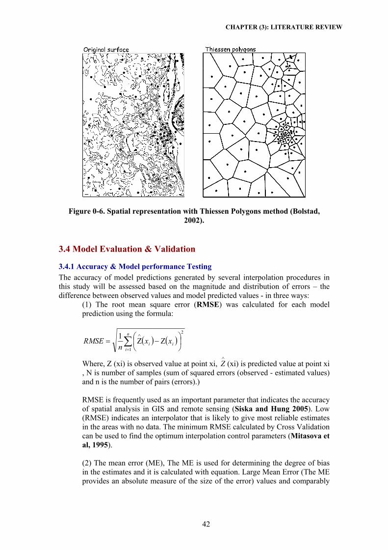
CHAPTER (3): LITERATURE REVIEW
42
Figure 0-6. Spatial representation with Thiessen Polygons method (Bolstad, 2002).
3.4 Model Evaluation & Validation
3.4.1 Accuracy & Model performance Testing The accuracy of model predictions generated by several interpolation procedures in this study will be assessed based on the magnitude and distribution of errors – the difference between observed values and model predicted values - in three ways:
(1) The root mean square error (RMSE) was calculated for each model prediction using the formula:
Where, Z (xi) is observed value at point xi, ∧
Z (xi) is predicted value at point xi , N is number of samples (sum of squared errors (observed - estimated values) and n is the number of pairs (errors).) RMSE is frequently used as an important parameter that indicates the accuracy of spatial analysis in GIS and remote sensing (Siska and Hung 2005). Low (RMSE) indicates an interpolator that is likely to give most reliable estimates in the areas with no data. The minimum RMSE calculated by Cross Validation can be used to find the optimum interpolation control parameters (Mitasova et al, 1995).
(2) The mean error (ME), The ME is used for determining the degree of bias in the estimates and it is calculated with equation. Large Mean Error (The ME provides an absolute measure of the size of the error) values and comparably
( ) ( )2
1
1 ∑=
∧
⎟⎠⎞
⎜⎝⎛ Ζ−Ζ=
n
iii xx
nRMSE

CHAPTER (3): LITERATURE REVIEW
43
large VE indicate larger discrepancies between predicted and observed values (Tatalovich, 2006). The ME formula as below
Where, Z (xi) is observed value at point xi, ∧
Z (xi) is predicted value at point xi, N is number of samples The overall performance of the interpolator is then evaluated by statistical means such as the root mean of squared residuals or mean error (ME) (Tomczak, 1998). Low root mean squared error (RMSE) indicates an interpolator that is likely to give most reliable estimates in the areas with no data. The minimum RMSE calculated by Cross Validation can be used to find the optimum interpolation control parameters (Mitasova et al, 1995). (3) Correlation (R) R (Correlation Coefficient) is the measure of the degree of relationship between the X (measured) and Y (predicted) variables. R2 (Coefficient of determination) explains the percent of the variability in Y (predicted) that can be explained by the regression equation. Correlation coefficients were calculated between observed and predicted values and between errors and observed values. Better model performance is indicated by higher coefficients between observed and predicted, and lower coefficients between errors and observed values. Further, the quantity R, called the linear correlation coefficient, measures the strength and the direction of a linear relationship between two variables. The linear correlation coefficient is sometimes referred to as the Pearson product moment correlation coefficient in honor of its developer Karl Pearson. The mathematical formula for computing R Where n is the number of pairs of data is:
Generally, the best model is the one that has standardized mean nearest to zero, the smallest root mean square prediction error. (Johnston et al., 2001).
3.4.3 Cross validation Cross validation is a model evaluation method for checking validity of the spatial interpolation method used. The most rigorous way to assess the quality of an output surface is to compare the predicted values for specified locations with those measured
( ) ( )∑=
∧
⎟⎠⎞
⎜⎝⎛ Ζ−Ζ=
n
iii xx
nME
1
1
( )( )( ) ( ) ( ) ( )2222 ∑∑∑∑
∑∑∑−−
−=
yynxxn
yxxynR

CHAPTER (3): LITERATURE REVIEW
44
in the field. It is not always possible to go back to the study area to collect an independent validation dataset. One solution is to divide the original dataset into two parts. One part can be used for modeling, that is, to create the output surface, and the other can be used for testing, that is, to validate the output surface. There are several validation techniques e.g. holdout set method, 5-fold, 10-fold, K-fold and N-fold. In N-fold cross-validation, the data set is split into N subsets of roughly equal size. The classification algorithm is them tested N times, each time training with N-1 of the subsets and testing with the remaining subset (Weiss & Kulikowski, 1991).
3.5 Software processing Many software packages exist for interpolation of point data. A distinction can be made between automatic processing and manual processing (processing with user intervention). Based on this literature review and the software available the following software may be considered for processing, as we find that ESRI ArcGIS (ESRI, 2009a) is the most widely used commercial GIS in the world and the most important module.
3.5.1 ArcMap ArcMap is the main component of ESRI’s ArcGIS suite of geospatial processing programs, and it is used primarily to view, edit, create, and analyze geospatial data. ArcMap allows the user to explore data within a data set, symbolize features accordingly, and create maps for clients. (Wikipedia, 2009b). Fig. 3-7 below presents the ArcMap window under ArcGIS 9.2 software that been utilized during the study.
Figure 0-7. ArcMap window and related features.

CHAPTER (3): LITERATURE REVIEW
45
3.5.2 ArcView ArcView 8.x and 9.x are part of the ArcGIS Desktop software suite. ArcView is the entry level of licensing offered, it is able to view & edit GIS data held in a flat file database or, through ArcSDE view data held in a relational database management system. Other licensing levels in the suite, namely ArcEditor and ArcInfo have greater functionality. All components are installed on the system, with only those that are licensed being made functional. (Wikipedia, 2009c).
3.6 Recommended interpolation methods in the study In practice, selection of a particular interpolation method should depend upon the configuration of the data set, the type of surfaces to be generated, and tolerance of estimation errors. In generating surfaces, a three step procedure is recommended: the first step is to evaluate the data set. This give idea on how data are spatial distributed, and may provide hints on which interpolation method should be used. The second step is adopted and applies an interpolation method which is most suitable to both the data set and the study objectives. The third step is compare the results using descriptive tools and determines the most stratifying result and the most suitable method. Burrough & McDonnell, 1998 state that when data are abundant most interpolation techniques give similar results. When data are sparse, the underlying assumptions about the variation among sampled points may differ and the choice of interpolation method and parameters may become critical. There are many interpolation methods available (Watson, 1992); (Burrough, 1986); (Lam, 1983); and (Ripley, 1981). Each of these methods works best for a particular data set because of its inherent assumptions and algorithm design for estimation. For a given data set, different interpolation methods may work best for different study objectives (i.e. smooth surface vs. accurate surface). There is no general method that is suitable for all problems: it depends on the nature of the variable and on the time-scale on which the variable is represented. According to (Tveito, 2007), climate reference maps should be based on the interpolation of absolute values. Taking into consideration several papers and studies regarding the comparison of interpolation methods and the best fitted models, where each study a/o paper is investigating a wide variety of spatial interpolation techniques, it can be briefed as following: In recent study in 2008 done by Mehrjardi and others titled as: Application of Geostastical Methods for Mapping Groundwater Quality in Azarbayjan Province, Iran. They have compared efficiency of three interpolation techniques included IDW, Kriging and cokriging for predicting of some groundwater quality indices such as: Na+, TH, EC, SAR, Cl- , Ca+2, Mg+2 and SO4, as a prerequisite of ecosystem management decisions is monitoring of soil and waters that geostatistics methods are one of the most advanced techniques for monitoring of them. The data were taken from 625 wells in Azarbayjan Province, Iran. After normalization of data, variograme was computed. Suitable model for fitness on experimental variograme was selected

CHAPTER (3): LITERATURE REVIEW
46
based on less RMSE value. Then the best method for interpolation was selected, using cross-validation and RMSE. The results showed that for all groundwater quality indices, cokriging performed better than other methods to simulate groundwater quality indices. Moreover, Coulibaly M. and S. Becker S. in 2007 have done a study named: Spatial Interpolation of Annual Precipitation in South Africa - Comparison and Evaluation of Methods. The data from 545 rainfall gauges were used to interpolate the spatial distribution of annual rainfall in South Africa. Several spatial interpolation methods (inverse distance weighting (IDW), ordinary Kriging, universal Kriging, and cokriging) were tested by variation analyses and cross-validation to determine the most suitable one. The best results were achieved by ordinary Kriging. Additionally, Christos G. and others in year 2010, have investigated in a study paper the Evaluation of Spatial Interpolation Techniques for Mapping Agricultural Topsoil Properties in Crete, as the aim of their work was to evaluate prediction maps created with interpolation for five common topsoil properties, namely organic matter, total CaCO3, electric conductivity (EC), Fe+2 content, and clay content in a Mediterranean agricultural system. 106 topsoil samples were collected on a 50 × 50 m2 grid and then analyzed in the laboratory. Three well-known spatial interpolation techniques, namely Ordinary Kriging (OK), Inverse Distance Weighting (IDW), and Radial Basis Functions (RBF) were applied for generating the prediction maps, which then were assessed for their accuracy and effectiveness with a new, independent set of samples. The results indicated that there was not a method clearly more accurate than the other methods for any of the tested properties. But IDW has shown better Goodness of prediction had positive values for Fe content and total CaCO3. Recent study named: Spatial Distribution of Groundwater Quality with Geostatistics (Case Study: Yazd-Ardakan Plain prepared by Mehrjardi M. and others in 2008, explored in their research that IDW, Kriging and cokriging methods were used for predicting spatial distribution of some Groundwater characteristics such as: TDS, TH, EC, SAR, Cl- and SO4. the data were related to 73 wells in Ardakan-Yaz plain. After normalization of data, variograme was drawn, for selecting suitable model for fitness on experimental variograme, less RSS value was used. Then using cross-validation and RMSE, the best method for interpolation was selected. Results showed that for interpolation of Groundwater quality, Kriging and cokriging methods are superior to IDW method; maps of Groundwater were prepared using cokriging Also, we can see that Sheikhhasan H. in 2006 has done a comprehensive study and evaluation of spatial techniques for rainfall estimation in his Master’s Thesis in Computer Science titled as A Comparison of Interpolation Techniques for Spatial Data Prediction. He has done a comprehensive study and evaluation of spatial techniques for rainfall estimation. The data were tested using three kinds of measurements, Residuals, RMSE, and prediction maps. As he has assured that there are a small number of projects that have provided a comparison and superiority of some spatial techniques over others. The objective of their thesis was to provide a comparison between eight interpolation and regression techniques for Rainfall Estimation. Finally the Predication maps made were clear that inverse distance weighted interpolations produced smoother maps.

CHAPTER (3): LITERATURE REVIEW
47
Further, Tatalovich Z. in 2006 has studied the performance of Thiessen-polygon and Kriging procedures from the standard GIS package in a paper called: Comparison of Thiessen-polygon, Kriging, and Spline Models of UV Exposure. The objective of his study was to identify model that produces least amount of uncertainties in predictions, and utilize that model to generate UV exposure estimates at non-sampled locations across United States. Input data included average global radiation measures computed from hourly data for period 1961-1990 for 215 stations in the U.S. The Spline model produced results with the smallest mean absolute error, smallest variance of error, smallest root mean square error, the highest correlation coefficient between the predicted and observed values and the smallest correlation between the errors and observed values. Moreover, a study prepared by Largueche F. in 2006 about Estimating Soil Contamination with Kriging Interpolation Method, where she has proved that Kriging is a useful tool to estimate the spatial distribution of ground pollutants in contaminated land. A spatial analysis has been carried out. It consists essentially of: Firstly a primary process of the data which means that histograms and an unprocessed representation of the pollutant’s distribution has been plotted for each contaminant, and secondly a graphic presentation of the pollution by using Kriging interpolation technique. In 2003 a paper prepared by Anderson S. titled as An Evaluation of Spatial Interpolation Methods on Air Temperature in Phoenix, AZ, where it reviews three methods of interpolation to be used on air temperature data from the Phoenix Metropolitan area. The air temperature measurements were taken at thirty-six discrete locations. Much of the geographical spatial analysis requires a continuous data set and this study is designed to create that surface. This study identifies the best spatial interpolation method to use for the creation of continuous data for air temperatures. The reviewed techniques include Spline, inverse distance weighting (IDW) and Kriging. A statistical assessment of the resultant continuous surfaces indicates that there is little difference between the estimating ability of the three interpolation methods with Kriging performing better overall. Whereas, paper presented by Meyer C. in 2003 titled as Evaluating water quality using spatial interpolation methods, in Pinellas County, Florida, U.S.A, to visualize the spatial trends of water quality monitoring data, spatial interpolation methods were applied to the chlorophyll and dissolved oxygen data from 45 fixed monitoring stations across the county. Investigation determined that inverse distance weighting IDW was the best interpolation method for the data. The IDW surfaces displayed overall trends and hotspots for extreme high and low values as it worked best with limited sample size and random data points. Recent paper prepared & published in International Journal of Environmental Science and Engineering by F. J. Moral García F.J. and others in 2010, titled as Geostatistical Analysis and Mapping of Ground level Ozone in a Medium Sized Urban Area in Badajoz, City southwest of Spain, where Ground-level tropospheric ozone is one of the air pollutants of most concern. Later, to evaluate the ozone distribution at the city, the measured ozone data (138 urban locations) were analyzed using Geostatistical techniques. During the exploratory analysis of data, it was revealed that they were distributed normally, which is a desirable property for the subsequent stages of the

CHAPTER (3): LITERATURE REVIEW
48
Geostatistical study. Yet and during the structural analysis of data, theoretical spherical models provided the best fit for all monthly experimental variograms. Finally, predictive ozone maps were derived for all points of the experimental study area, by use of Geostatistical algorithms (Kriging) and high prediction accuracy was obtained in all cases as cross-validation showed. A paper in year 2007 prepared by Ibrakhimov M. and others titled as Spatial and temporal distribution and influence on soil Stalinization in Khorezm region (Uzbekistan, Aral Sea Basin), has analyzed the temporal dynamics of GW table and salinity in Khorezm, a region of Uzbekistan which is situated on the lower Amu Darya River in the Aral Sea Basin and suffering from severe soil salinization. Data of GW table and salinity were measured during 1990–2000 in 1,972 wells, covering the entire region. Over the entire area, GW was only moderately saline. However, GW levels were generally very shallow and thus likely to prompt secondary soil salinization. Maps interpolated from the regional dataset revealed that GW was significantly shallower and more saline in the western and southern parts of Khorezm using Kriging interpolation method. Shamsudduha M. in 2007, investigated in a study called: Spatial Variability and Prediction Modeling of Groundwater Arsenic Distributions in the Shallowest Alluvial Aquifers in Bangladesh, the Spatial variability of arsenic in groundwater has been examined by semivariogram analysis that revealed high degree of small-scale spatial variability in alluvial aquifers. Small-scale variability of arsenic concentrations, indicated by high “nugget” values in semivariograms, is associated with heterogeneity in local-scale geology and geochemical processes. In non-sampled locations, arsenic concentrations have been predicted using both deterministic and stochastic prediction methods. Natural neighbor (NN) method predicted better than inverse distance to power (IDW) method, and small-scale variations of arsenic concentrations are preserved. Predicted results are evaluated by cross-validation, mean prediction error, and root mean square methods. Ordinary Kriging (OK) method on the untransformed arsenic data and their residual values performed considerably in predicting spatial arsenic distributions on regional scale. In 2005, Salih M. and others in a study titled as Spatial correlation between radon in groundwater and bedrock uranium: GIS and Geostatistical analyses; described approaches to create surface maps of radon in groundwater based on measurements of radon in drilled bedrock wells at unevenly distributed sites and uranium bedrock maps from the South East of Sweden. Geostatistical techniques of inverse distance weighted (IDW), Kriging and cokriging were compared in terms of their interpolation power and correlation between the produced radon in the water layer and the bedrock uranium layer. Good interpolation layers (with least root mean square errors RMSE) were obtained by Kriging. However, the kriged radon surface showed poor correlation with bedrock uranium layers. The best radon in water layer that match with uranium in bedrock layer was produced using IDW interpolator. In parallel, Mueller R. Jr. in his study in 2005 called: Utilizing Geographic Information Science Advancements for Bathymetric Mapping and Dredging Assessment of a Small Urban Lake in Southeastern Minnesota, which is a small Mississippi River floodplain lake in Winona, Minnesota USA. Lake Winona was the site of recent dredging operations aimed at decreasing littoral zone areas to reduce

CHAPTER (3): LITERATURE REVIEW
49
plant growth and stunted fish populations. To assess potential effectiveness of dredging operations, bathymetric data were collected with a Garmin depthfinder and GPS unit, and interpolation techniques to produce Lake Morphometric characteristics (splining, Kriging, and inverse distance weighting (IDW)) were compared within ESRI’s ArcMap 9.0. All interpolation methods produced similar outputs for cross validation statistical comparisons, although Kriging produced the best predictive output of actual bathymetric contouring for Lake Winona. But Valley R. D. and others in 2004, in their research: Evaluation of alternative interpolation techniques for the mapping of remotely-sensed submersed vegetation abundance, have evaluated a hydroacoustics global positioning system to map the percent of the water column occupied by submersed vegetation (referred to here as biovolume) in three Minnesota (USA) lakes. As they evaluated the relative accuracy and precision of digital biovolume maps produced by three interpolation methods (inverse distance weighted (IDW), Kriging and Spline) after using a non-parametric regression smoother to remove a non-linear depth trend. Interpolated predictions with all methods were relatively accurate in all lakes; however, precision varied among lakes. In all cases, Kriging interpolation produced the best predictions when compared with observations in independent verification data sets. Comprehensive paper released in 1999 and prepared by Hartkamp, A.D. and others titled as Interpolation Techniques for Climate Variables. NRG (Natural Resources Group)-GIS Series 99-01. Mexico has examined statistical approaches for interpolating climatic data over large regions, providing a brief introduction to interpolation techniques for climate variables of use in agricultural research, as well as general recommendations for future research to assess interpolation techniques. Three approaches: 1) inverse distance weighted averaging (IDWA), 2) thin plate smoothing splines, and 3) co-kriging; were evaluated for a 20,000 km2 square area covering the state of Jalisco, Mexico. Validation of the surfaces using two independent sets of test data showed no difference among the three techniques for predicting precipitation. For maximum temperature, splining performed best. Taking into account valued error prediction, data assumptions, and computational simplicity; the results recommended using of thin-plate smoothing Spline for interpolating climate variables. In conclusion, the techniques assessed previously and that will be practiced in the study are deterministic interpolation methods of SPLINE and INVERSE DISTANCE WEIGHTING (IDW) and the stochastic method of KRIGING in an effort to retain actual measurement in a final surface. Each method selected requires that the exact data values for the sample points are included in the final output surface.

CHAPTER (4): METHOD AND MATERIALS
50
CHAPTER (4): METHOD AND MATERIALS
4.1 Data employed The dataset comprised of three categories, groundwater quality parameter (Chloride (Cl-), Groundwater level (WL), and meteorological rainfall data. The dataset obtained in years from 2000 – 2007 from Palestinian Water Authority (PWA) and Coastal Municipalities Water Utility (CMWU) data bank's departments. In this chapter, the municipal well lists which were obtained from the PWA & CMWU; it was difficult to distinguish between municipal wells and domestic wells. It was found that there were some domestic wells (private wells) used by the municipality for some time. The evaluation only considered the working wells while there were many wells recently closed due to increasing salinity in the water or damaging and faulting of the mechanical parts of these wells. Appendix 1 shows also a summary of municipal wells and some of the domestic wells (use for domestic purposes but not belongs to the municipality) in each Governorate.
4.1.1 Groundwater Quality (Chloride - Cl- in mg/l) Water quality in Gaza is tested by different agencies for different reasons. The Ministry of Health (MoH) tests all of the approximately more than 130 Municipal wells twice a year (during June/July and Jan. /December months) for the major ions, nitrates, and coliform to insure that the drinking water is safe for public consumption. The MoA tests more than 400 wells twice a year for Chloride and Nitrate and some additional ions to assess the quality of the irrigation water in Gaza. In addition, the United Nations Welfare Relief Agency (UNWRA) tests their wells on a regular basis. Reportedly this testing is similar to that of the MoH. UNWRA administers the drinking water wells in the refugee camps, yet it will not be considered in the study (CAMP, 2000). It is worth mentioning that measurements in 2001, 2003, 2005 & 2007 were considered in the study. Reasons for consistent data, sampling accuracy, regular monitoring, harmonized wells development and extension, were behind choosing the Chloride concentration in mg/l as testing groundwater quality parameter, though these years to be briefed as following: The following table 4-1 details the study wells in 2001 and Fig. 4-1 below demonstrates the distribution of municipal wells over Gaza Strip's governorates, as more details about Chloride dataset in year 2001 can be found in Appendix 2.1 - Chloride Dataset in 2001.
Table 0-1. Summary of Chloride dataset in year 2001 Study Area Data in 2001 No. No. of Total Wells in Gaza Strip in 2001 71 No. of Wells used for Calibration 10 No. of Wells used for Modeling 61
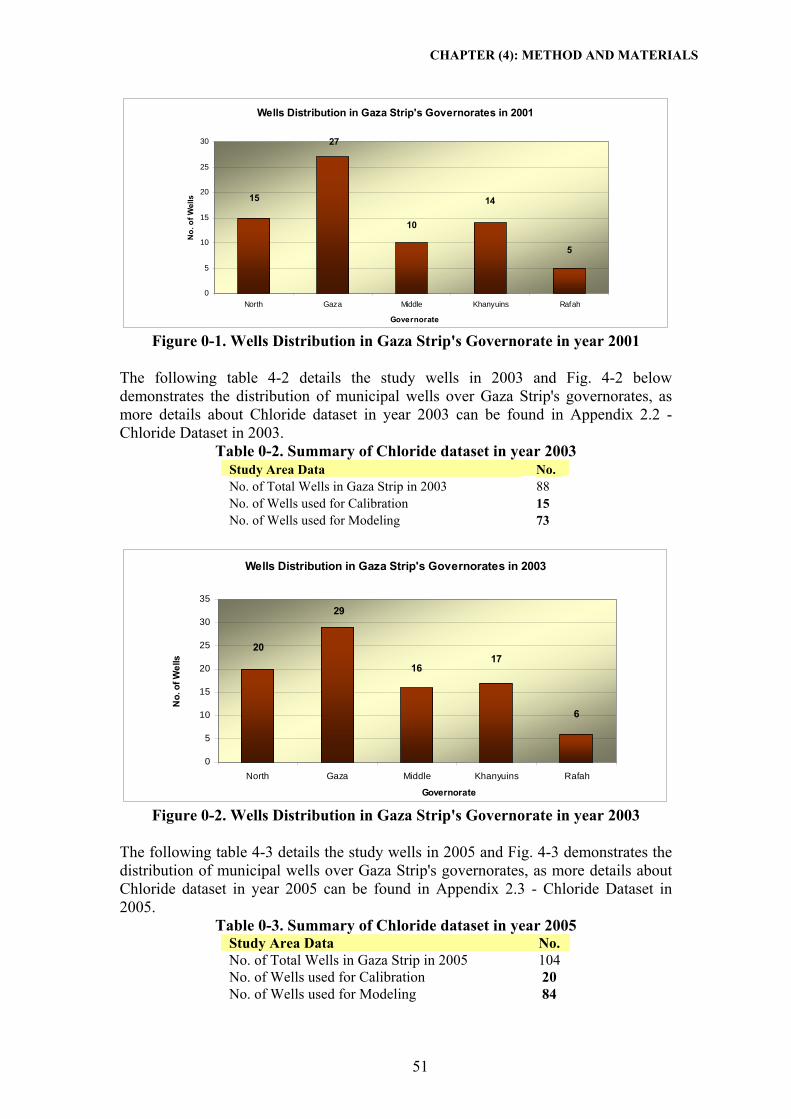
CHAPTER (4): METHOD AND MATERIALS
51
Wells Distribution in Gaza Strip's Governorates in 2001
15
27
10
5
14
0
5
10
15
20
25
30
North Gaza Middle Khanyuins Rafah
Governorate
No.
of W
ells
Figure 0-1. Wells Distribution in Gaza Strip's Governorate in year 2001
The following table 4-2 details the study wells in 2003 and Fig. 4-2 below demonstrates the distribution of municipal wells over Gaza Strip's governorates, as more details about Chloride dataset in year 2003 can be found in Appendix 2.2 - Chloride Dataset in 2003.
Table 0-2. Summary of Chloride dataset in year 2003 Study Area Data No. No. of Total Wells in Gaza Strip in 2003 88 No. of Wells used for Calibration 15 No. of Wells used for Modeling 73
Wells Distribution in Gaza Strip's Governorates in 2003
20
29
16
6
17
0
5
10
15
20
25
30
35
North Gaza Middle Khanyuins Rafah
Governorate
No.
of W
ells
Figure 0-2. Wells Distribution in Gaza Strip's Governorate in year 2003
The following table 4-3 details the study wells in 2005 and Fig. 4-3 demonstrates the distribution of municipal wells over Gaza Strip's governorates, as more details about Chloride dataset in year 2005 can be found in Appendix 2.3 - Chloride Dataset in 2005.
Table 0-3. Summary of Chloride dataset in year 2005 Study Area Data No. No. of Total Wells in Gaza Strip in 2005 104 No. of Wells used for Calibration 20 No. of Wells used for Modeling 84

CHAPTER (4): METHOD AND MATERIALS
52
Wells Distribution in Gaza Strip's Governorates in 2005
22
9
21
29
23
0
5
10
15
20
25
30
35
North Gaza Middle Khanyuins Rafah
Governorate
No.
of W
ells
Figure 0-3. Wells Distribution in Gaza Strip's Governorate in year 2005
Table 4-4 below details the study wells in 2007 and Fig. 4-4 below demonstrates the distribution of municipal wells over Gaza Strip's governorates, as more details about Chloride dataset in year 2007 can be found in Appendix 2.4 - Chloride Dataset in 2007.
Table 0-4. Summary of Chloride dataset in year 2007 Study Area Data No. No. of Total Wells in Gaza Strip in 2001 129 No. of Wells used for Calibration 23 No. of Wells used for Modeling 106
Wells Distribution in Gaza Strip's Governorates in 2007
25
11
28
40
25
0
5
10
15
20
25
30
35
40
45
North Gaza Middle Khanyuins Rafah
Governorate
No.
of W
ells
Figure 0-4. Wells Distribution in Gaza Strip's Governorate in year 2007
4.1.2 Groundwater water level (WL in meters) Groundwater level Data was obtained from PWA-Water Resources Directorate and CMWU-Data Bank. The data collected was mainly concerned in years 2000-2007.

CHAPTER (4): METHOD AND MATERIALS
53
The collected data were based on average values (yearly records in meters) for each year through different readings through the same year. In terms of historical hydrogeological data related to the depth of groundwater levels, it was noted that the water level was above the ground level with 5-15 meters, and there was a clear slope and flow of groundwater encountered from the southeastern side to the northwestern with no observations of any phenomena related to any upcoming issues. (Yaqoubi, 2006). Two types of wells used to monitor the groundwater level: 1) Monitoring Wells, which can be municipal or domestic wells with shallow depths ranged down to 40 meters. The other type is 2) Piezometer Wells, which mainly were constructed for monitoring purposes and depths range from 20-200 m. It was clear that after several years of operation, part of the wells encountered different function-affecting problems including clogging, scaling, fouling, and high turbidity. The problems mentioned previously may affect the function of Monitoring and Piezometer wells and the accuracy of groundwater level monitoring. The active wells are shallow wells and typically their screens are 10-20 m below the water table. Of these wells, about 140 monitoring wells and 39 piezometric wells are presently used to monitor the water levels every month. The agriculture wells of about 10 inches diameters are used as water level monitoring wells. The total depth of most of the wells is not defined clearly. Generally, the total penetrated saturated thickness of these wells is ranging between 30 and 40 m. Most of the piezometric wells are located mainly along the coastal zone and range in depth from 20 to 200 m. Many of these wells have screens at different depths. The piezometric wells have deteriorated and many of these wells have been damaged. (Mogheir, 2003). It is worth mentioning that the records in 2001, 2003, 2005 & 2007 were considered in the study. Reasons for consistent data, sampling accuracy, regular and monitoring activities were behind choosing of the said years. Table 4-5 illustrates the number of monitoring and piezometer wells in Gaza Strip through the different years of study. More details about water level dataset will be found in Appendix 3 – Water Level Dataset:
Table 0-5. Number of wells used for Water level study dataset Description / Year 2001 2003 2005 2007
No. of Monitoring Wells 96 88 71 66 No. of Piezometer Wells 15 14 34 33
Total No. of Wells used for Groundwater Water Level Monitoring 111 102 105 99
During our investigation and exploring the Water Level data, the following were raised as points of interests:
1) Full records of water level were decreased during years from 2001 to 2007 (111 to 99) in many monitoring wells either due to lack of frequent maintenance and shortage of spare parts needed for rehabilitation process or

CHAPTER (4): METHOD AND MATERIALS
54
due to accessibility issues under security concerns considered as dangerous zone.
2) No. of Piezometer wells were increased in 2004/2005 under a program funded by USAID and implemented through PWA under IAMP study outputs.
4.1.3 Meteorological data (Rainfall in mm) In Gaza Strip there are 12 rainfall stations distributed through different governorates, these stations are operated by ministry of agriculture and data obtained from these stations are entered manually in Palestinian water authority database. The data was obtained from PWA and CMWU data bank departments as yearly average rainfall data in mm for the years from 2000 to 2007. The records in PWA and MOA were based on monthly rainfall depth collected measurements from rain gauges that start in July of particular year and ends in June of next year. It is worth mentioning that the records in 2000/01, 2002/03, 2004/05 & 2006/07 were considered in this study as shown in table 4-6. Reasons for consistent data, sampling accuracy, regular and monitoring were behind choosing the said years. More details about the rainfall data can be found in Appendix 4 – Rainfall Dataset:
Table 0-6. Rainfall dataset in study years (mm/year) Station_Name 00-01' 02-03' 04-05' 06-07' Beit Hanoun 497.50 801.50 358.70 509.90 Beit Lahia 490.40 724.00 320.60 530.30 Jabalia 540.00 692.60 345.50 536.70 Shati 478.90 627.00 296.60 469.00 Gaza City 511.90 599.00 316.00 501.20 Tuffah 533.40 653.50 345.40 545.50 Gaza South 563.60 790.70 323.60 388.20 Nusseirat 558.30 446.20 405.00 403.00 Deir Al Balah 550.50 372.60 345.50 418.00 Khan Younis 381.00 298.00 373.00 252.00 Khuzaa 284.30 261.20 367.70 256.10 Rafah 308.00 220.80 360.20 225.00
4.1.4 ArcGIS documents The major file needed to assess the extent of any data in space and time was the GazaStrip.shp file (National Grids-Palestinian Grid 1923) which was obtained from CMWU-data bank, which details the boundaries of Gaza Strip where the spatial extension ends. The study area matches these maps which cover the entire Gaza Strip area.
4.2 Dataset Processing The data required some processing before it could be used in ArcGIS. First, the data was opened using Excel and saved in several Excel spreadsheets. The dataset was

CHAPTER (4): METHOD AND MATERIALS
55
verified, sieved and stored in three main categories: Water Quality data, Water Level Data, and Rainfall Data. In each category, the dataset was compiled into four main tables for years of 2001, 2003, 2005 and 2007. As for the Water Quality data, the information stored was mainly about Well_ID, Well_Name, Municipality, Governorate, X, Y data (Longitude, Latitude), and yearly average of Chloride Concentration in mg/l. The Water Level data, it was about Well_ID, Well_Type, X, Y data (Longitude, Latitude), and yearly average of Water Level in meters, while, the Rainfall data was stored as Station_Location, Station_Name, X, Y data (Longitude, Latitude), and yearly average of rainfall amount in mm. The above selected data, were organized in several Excel spreadsheets and saved as a DBF 4 *.dbf files. These file were imported into the geodatabase and then added to an ArcMap document. But, prior to any temporal analyses, the aforementioned data were checked for the distributional assumptions and descriptive statistics, as exploratory spatial data analysis was applied for the chloride, water level and rainfall to check data consistency, removing outliers and identifying statistical distribution where data came from. It is worth mentioning that during the exploratory phase, transformation of data shall be a necessity once the data was not distributed normally, as the goal of transformations is to normalize the available datasets we have, as it enable us to re-check the different datasets for normality after performing the transformation whose distribution is most normal (log transformation is the technique that shall be used in the Geostatistical Analysis tools), as stated in (Lutkepohl, H., 2009) that for a range of economic variables substantial forecast improvements from taking logs are found if the log transformation actually stabilizes the variance of the underlying series. It can be damaging for the forecast precision if a stable variance is not achieved. Furthermore, statistics provide additional numerical information to confirm the graphical tendencies shown with the histograms (Johnston et al., 2001).
4.2.1 Groundwater Quality (Chloride (Cl-) in mg/l) Descriptive statistics of the Chloride dataset can be demonstrated in table 4-7 as following:
Table 0-7. Statistics analysis of Chloride Dataset Year Count Min. Max. Mean Median Skew SD Kurtosis2001 71 35.4 1,175.75 394.68 308.40 0.783 297.873 2.592 2003 88 29.32 2,009.65 428.31 305.90 1.456 353.189 6.082 2005 104 43.06 2,031.00 476.00 350.08 1.459 397.918 5.461 2007 129 35.14 2,077.00 527.17 444.60 1.600 424.472 5.865 The chloride ion concentration dataset varies from less than 250mg/l in the sand dune areas as the northern and south-western area of the Gaza Strip to about more than 1500 mg/l along the coastal areas as shown in the figures listed in Appendix 8. The general trend of chloride concentration is notably increasing due to many factors but not limited to freshwater source represented in rainfall intensity, seawater intrusion, high pumping capacities, and deep penetrated wells.
Moreover, it is clear that in all years (2001, 2003, 2005, and 2007) the data are not quite normally distributed due to positive skewed values increasing gradually (0.783,

CHAPTER (4): METHOD AND MATERIALS
56
1.456, 1.459, and 1.600. The distribution showed positive peaked shape in 2001, 2003, 2005 and 2007 with kurtosis of 2.5915, 6.082, 5.461, and 5,865 respectively. More details can be referred to Appendix 8.
4.2.2 Groundwater water level (WL in meters) Descriptive statistics of the Water Level dataset can be demonstrated in table 4-8 as following:
Table 0-8. Statistics analysis of Water Level Dataset Year Count Min. Max. Mean Median Skew SD Kurtosis2001 111 -6.469 12.885 -0.121 -0.066 1.595 2.452 8.470 2003 102 -8.173 9.601 -0.452 -0.242 -0.009 2.593 3.572 2005 105 -10.055 10.058 -0.497 -0.190 -0.042 2.900 3.430 2007 99 -12.797 10.453 -0.925 -0.438 -0.394 3.313 4.176 Water level dataset in years of 2001, 2003, 2005 and 2007 have demonstrated obvious problem in the northern and southern side of Gaza Strip due to imbalance between replenishment and consumption averages with comprehensible groundwater levels drop with reference to MSL. As shown below in Figs 4-5, 4-6, 4-7, and 4-8 the drop increased from 6.469 down to 12.797 meters below MSL. The situation is worse in the southern side due to less replenishment process escorted by low annual precipitations as the recharge rate is about 25% in the low porous area like the eastern part of the Gaza Strip, and about 75% in porous area where the sand dunes are still found in the north and south of GS (CMWU, 2008) and higher population demand with more urban expansions. Statistically, the distribution of 2001 data is characterized by positive high skewness (1.595) and really high peaked positive kurtosis (8.470) due to infrequent extreme deviations. In 2003 & 2005, we can define the data are entirely normally distributed due to negative skewness near zero of (-0.009 & -0.042), while we have left sided distributed data in 2007 with negative skewness (-0.394) and positive kurtosis (4.176).
Figure 0-5. Histogram Graph for Water Level in year 2001

CHAPTER (4): METHOD AND MATERIALS
57
Figure 0-6. Histogram Graph for Water Level in year 2003
Figure 0-7. Histogram Graph for Water Level in year 2005

CHAPTER (4): METHOD AND MATERIALS
58
Figure 0-8. Histogram Graph for Water Level in year 2007
4.2.3 Meteorological data (Rainfall in mm) Descriptive statistics of the Rainfall dataset can be demonstrated in table 4-9 as following:
Table 0-9. Statistics analysis of Rainfall Dataset
Year Count Min. Max. Mean Median Skew SD Kurtosis2000/01 12 284.30 563.60 474.82 504.7 -1.213 96.924 0.154 2002/03 12 220.80 801.50 540.59 613.0 -0.339 210.477 -1.518 2004/05 12 296.60 405.00 346.48 345.5 0.219 29.433 0.220 2006/07 12 225.00 545.50 419.58 443.5 -0.672 117.947 -1.066
The rainfall dataset demonstrated close rainfall dataset average but with high rainfall intensity occurred in 2002/03 year unlike the average occurred in 2004/05. Moreover, there is a regional trend in the rainfall dataset where the general concentrations increase toward the north from south of the Gaza Strip. The distribution of 2000/01 data is characterized by negative skewness of (-1.213) tended to the left side and positive kurtosis of (0.154) with peaked distribution. Flat distribution of 2002/03 data were noticed due to negative kurtosis with negative skewness of (-0.339). The 2004/05 data have shown normal flat distribution characterized by positive skewness (0.219) and low positive kurtosis (0.220). The distribution of 2006/07 showed flat distribution of negative kurtosis (-1.066) and slight left sided location of data of negative skewness (-0.672). More details regarding Rainfall dataset histograms and normalization process can be found in Appendix 9.

CHAPTER (4): METHOD AND MATERIALS
59
4.3 Methods The dataset including water quality parameters & rainfall amounts were imported into ESRI ArcMap software. The ESRI Geographic information system (GIS) was used for the construction of creation of the interpolation surfaces through applying the ‘Geostatistical Analyst’ extensions of ArcGIS 9.2 software package. ESRI ArcGIS (ESRI, 2009c) is the most widely used commercial GIS in the world and the most important module, ArcMap, supports most interpolation methods except linear regression modeling which should be done using an external statistical package. ESRI ArcMap is very powerful for visualization and processing with user intervention (Sluiter, 2008). GIS modules are described to spatially interpolate data of radon concentration in water. Two interpolation techniques, Spline, inverse distance weighted (IDW) and Kriging, used in the present study are briefly summarized below: The application of any interpolation method for the spatial interpolation of data assumes a normal distribution. It is a pre-requisite to transform skewed data into a normal distribution before applying to any geostatistical analysis. Logtransformation is one of the widely used methods for data normalization. Three interpolation procedures used to generate a set of predicted values at known locations. In each instance the predicted values were generated by systematically removing some of the input data (Calibration data) for Chloride, WL, and rainfall then calculating their values based on other data (Modeling data), where the goal of the study geostatistical analysis is to predict values where no data have been collected. IDW, Kriging and Spline (RBF) procedures are evidently very different not only statistically, but also in terms of computational complexity, and their ability to incorporate additional variables, all of which may differentially affect the predictions. One way to assess the performance of different exposure models would be to examine the magnitude and distribution of prediction errors.
4.3.1 Applied Interpolation Techniques
4.3.1.1 Spline (RBF) Spline which described as RBF is moderately quick deterministic interpolators that are exact. There is no assessment of prediction errors. The method provides prediction surfaces that are comparable to the exact form of Kriging & IDW. Radial Basis Functions do not allow you to investigate the autocorrelation of the data, making it less flexible and more automatic than Kriging & IDW. Radial Basis Functions make no assumptions about the data. The RBF (Spline) interpolation was performed and the produced layer was compared. Finally, and as per the process above, cross validation parameters (error estimates) and correlation coefficients between the generated models were tabulated for comparison and evaluation.
4.3.1.2 IDW The points are weighted during interpolation such that the influence of one point relative to another is a function of inverse distance. Weighting is assigned to points through the use of a weighting power and the radius object. The greater power means
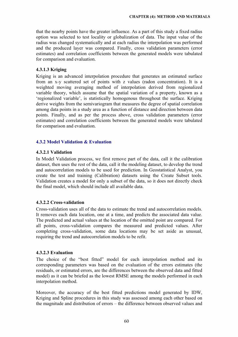
CHAPTER (4): METHOD AND MATERIALS
60
that the nearby points have the greater influence. As a part of this study a fixed radius option was selected to test locality or globalization of data. The input value of the radius was changed systematically and at each radius the interpolation was performed and the produced layer was compared. Finally, cross validation parameters (error estimates) and correlation coefficients between the generated models were tabulated for comparison and evaluation.
4.3.1.3 Kriging Kriging is an advanced interpolation procedure that generates an estimated surface from an x-y scattered set of points with z values (radon concentration). It is a weighted moving averaging method of interpolation derived from regionalized variable theory, which assume that the spatial variation of a property, known as a ‘regionalized variable’, is statistically homogenous throughout the surface. Kriging derive weights from the semivariogram that measures the degree of spatial correlation among data points in a study area as a function of distance and direction between data points. Finally, and as per the process above, cross validation parameters (error estimates) and correlation coefficients between the generated models were tabulated for comparison and evaluation.
4.3.2 Model Validation & Evaluation
4.3.2.1 Validation In Model Validation process, we first remove part of the data, call it the calibration dataset, then uses the rest of the data, call it the modeling dataset, to develop the trend and autocorrelation models to be used for prediction. In Geostatistical Analyst, you create the test and training (Calibration) datasets using the Create Subset tools. Validation creates a model for only a subset of the data, so it does not directly check the final model, which should include all available data.
4.3.2.2 Cross-validation Cross-validation uses all of the data to estimate the trend and autocorrelation models. It removes each data location, one at a time, and predicts the associated data value. The predicted and actual values at the location of the omitted point are compared. For all points, cross-validation compares the measured and predicted values. After completing cross-validation, some data locations may be set aside as unusual, requiring the trend and autocorrelation models to be refit.
4.3.2.3 Evaluation The choice of the “best fitted” model for each interpolation method and its corresponding parameters was based on the evaluation of the errors estimates (the residuals, or estimated errors, are the differences between the observed data and fitted model) as it can be briefed as the lowest RMSE among the models performed in each interpolation method. Moreover, the accuracy of the best fitted predictions model generated by IDW, Kriging and Spline procedures in this study was assessed among each other based on the magnitude and distribution of errors – the difference between observed values and

CHAPTER (4): METHOD AND MATERIALS
61
model predicted values as following: The root mean square error (RMSE) and the mean error (ME) were calculated for each model prediction. In addition to the R (Correlation Coefficient) that was measured between the measured and predicted variables as well as R2 (Coefficient of determination). The overall approach and methodology can be briefed in Fig. 4-9 next, where it illustrates the stages that the study went through and the modeling techniques applied for the three datasets for the different study years.

CHAPTER (4): METHOD AND MATERIALS
62
Figure 0-9. Study flowchart in selection the best interpolation method
Kriging Method
INTERPOLATION METHOD ArcGIS – ArcMap software Spatial Analyst Extension
Spline Method IDW Method
Kriging Method Tension/Regularize Smoothing Factor
Cross Validation
Lowest RMSE &
ME Lowest RMSE &
ME
Exploratory Data Analysis
Distribution & skewness
Semivariogram modeling
No
Yes
Power Exploring
Yes
No
Best Model Best Model
Cross Validation
Lowest RMSE &
ME
Best Model
Yes
No
CROSS VALIDATION Lowest RMSE & ME among
all best models
Surface Generation
No
Yes
Best Interpolation Method

CHAPTER (5): RESULTS & DISCUSSIONS
63
CHAPTER (5): RESULTS & DISCUSSIONS
5.1 Introduction The main objective of this study is to evaluate the spatial representation of groundwater data (Chloride & Water level) and meteorological data (Rainfall) in GS under the current different collection monitoring system dataset so as to optimize the interpolation methods or techniques examined in order to be utilized for accurate surface representation of areas with missing data points along with setting up recommendation for the future monitoring programme of GS aquifer. The quality of the interpolation methods are assessed by evaluating various prediction errors that are derived from the cross validation process (Coulibaly & Becker, 2007). The estimated value is then compared to the measured one for error estimation; three of the five types of prediction errors presented by Johnston et al. (2001) were taken into consideration.
5.2 Interpolation Application Specifically a statistical summary of the groundwater quality properties (Chloride and Water Level dataset) and Rainfall dataset was presented in Chapter 4. Based on their skewness and histogram, some of the data were normalized using logarithmic transformation. After data normalizing (once needed), experimental semivariogram, powering and smoothing factors were computed and recorded. The best model for fitting on experimental semivariogram, powering and smoothing was selected based on less RMSE value and other supporting factors like ME value. In order to validate the results obtained through applying the selected above different interpolation methods, of the total available dataset, few samples were randomly selected but geographically covering the whole dataset and kept as calibration dataset. They are not used for prediction or semivariogram estimation, so it is possible to compare predicted points with independent observations. In this study two test sets were used. The resulted surface mapping were evaluated using the cross-validation process, the resulted predicted data was compared with the measured data (calibration) and was subjected to correlation investigation. The best calibrated model that will be used for final surface map was selected based on highest correlation (R2) among all. It is really important to mention that all trials and fitting techniques results can be found in Appendix 11 (Chloride dataset), Appendix 12 (Water level Dataset), and in Appendix 13 (Rainfall Dataset) where in these appendixes the recommended final parameters that were optimized and recorded for the Kriging, IDW, and Spline (RBF) interpolation methods were highlighted. The Spline (RBF) method had two categories with optimizing factor to choose, while in the IDW method the smoothing factor along with powering parameter were verified. In the Kriging, different semivariogram parameters were tackled like partial sill, nugget, lag size, and smoothing factor for modeling techniques. Where the combination and the trails of the above multi associated parameters in the different interpolation methods is to interpolate a map that reflects more accurate predicted values and surface smoothing.

CHAPTER (5): RESULTS & DISCUSSIONS
64
Moreover, it is better to point out that in the interpolation mechanism, the objects are rasterized into two-dimensional images from their corner points (vertices), all the pixels between those points are filled in by the defined interpolation algorithm (Spline, IDW or Kriging), which determines their attributes as described in the creation of new values that lie between known values, and that’s what happened clearly in the above cases and results. Finally, couple of factors has already affected the interpolation process and gaining more reliable predicted data:
(1) Unreasonable distribution of monitoring points. (2) Monitoring frequency is roughly unreasonable. (3) Monitoring tools are out of date and measure errors existed. (4) High risks of data storage loss.
5.3 Results
5.3.1Chloride Dataset Results
5.3.1.1 2001 dataset The Chloride dataset was divided into two sets of data, modeling data and calibration data. The modeling data (61 samples) as shown in (Appendix 5.1 - Chloride Modeling Dataset in 2001) was applied in the three interpolation techniques, yet the Calibration dataset used can be demonstrated in table 5-1 below. Each interpolation technique was best fitted in the validation process, was evaluated through cross-validation process using calibration data with total no. of 10 samples.
Table 0-1. Calibration dataset of Chloride dataset for year 2001
Well_ID Well_Name X Y Cl_01
C_76 Industrial_Area_Well 104667.09 104336.57 578.90 D_73 Salateen_Well 101036.18 106827.16 70.75 D_70 Sheikh_Radwan_No._12 101440.34 105833.46 99.05 R_162CA Sheikh_Radwan_No._4 98867.35 104590.00 280.00 R_254 Sheikh_Ejleen_No._2 96540.88 102055.55 407.65 S_69 Abu_Merwan_Well 91769.92 90702.26 466.00 G_30 Hertani_Well 91478.84 95975.57 973.70 L_176 El_Sha'e _Old_Southern_Well 82187.00 83276.00 779.05 L_179 Western_well 85572.00 87460.00 650.00 P_138 Abu_Zohri_Well 78773.00 79764.00 128.60 The models for 2001 dataset were subjected for fitting process based on experimental semivariogram, powering and smoothing process and trails. As it can be summarized in the table 5-2, where the final models were selected based on least RMSE value.

CHAPTER (5): RESULTS & DISCUSSIONS
65
Table 0-2. Summary of Validation results for Chloride in year 2001
Measurements of Errors Spline IDW Kriging Mean: -15.82 -10.99 0.016 Root-Mean-Square: 206.2 187.5 195.7
As we can find in Fig. 5-1 the summary of statistical errors for Chloride in Year 2001 resulted from applying Kriging, Spline (RBF), and IDW interpolation methods.
(a) (b)
(c)
Figure 0-1. Prediction error statistics Vs Measured for Chloride in Year 2001 resulted from: (a) Kriging, (b) Spline (RBF), and (c) IDW interpolation methods
The best fitted above models were further evaluated using the calibration dataset, the results was summarized in table 5-3 and table 5-4.

CHAPTER (5): RESULTS & DISCUSSIONS
66
Table 0-3. Predicted values vs. measured Chloride values for year 2001
Well_ID Well_Type Cl_01 Spline IDW Kriging
Measured Predicted C_76 Industrial_Area_Well 578.90 291.08 313.17 339.20 D_73 Salateen_Well 70.75 80.49 85.36 72.40 D_70 Sheikh_Radwan_No._12 99.05 95.77 96.67 103.52 R_162CA Sheikh_Radwan_No._4 280.00 531.53 503.84 567.45 R_254 Sheikh_Ejleen_No._2 407.65 297.52 333.79 295.09 S_69 Abu_Merwan_Well 466.00 544.29 536.44 611.03 G_30 Hertani_Well 973.70 953.46 1018.40 1073.71 L_176 El_Sha'er_Old_Southern_Well 779.05 453.88 454.89 375.12 L_179 Western_well_ 650.00 561.47 473.07 444.63 P_138 Abu_Zohri_Well 128.60 343.60 301.78 365.92
Table 0-4. Summary of Cross Validation values for Chloride in year 2001 Measurements of Correlation Spline IDW Kriging
R 0.791 0.811 0.721
R2 0.625 0.658 0.520 Figure 5-2 below illustrates the tendency of each predicted values resulted from applying the three interpolation methods against the measured values for Chloride dataset in year 2001.
Predicted Values Vs Measured
0.00
200.00
400.00
600.00
800.00
1,000.00
1,200.00
C_76
D_73
D_70
R_162
CAR_2
54S_6
9G_3
0L_1
76L_1
79P_1
38
Well ID
Chl
orid
e C
once
ntra
tion
in m
g/
MeasuredSplineIDWKriging
Figure 0-2. Correlation Analysis for Chloride in Year 2001

CHAPTER (5): RESULTS & DISCUSSIONS
67
It is useful to clarify that the absolute value of errors (R) shows strong positive correlation with the magnitude of the Chloride predicted values at year 2001 as shown in table 5-4. While during the interpolation process and as shown in Fig 5-2, the predicted values at P_138 and R_162CA wells went underestimated unlike the L_179 well which was overestimated, in view of the fact that the interpolation process was affected by nearby locally extreme modeled values in which they were surrounded spatially by smaller values. As in this situation, there will be huge spatial variation among observations over a short distance. Yet, one strong factor can be added to this variation is the presence of local measuring error that associated in this case during the sampling process.
5.3.1.2 2003 dataset The Chloride dataset was divided into two sets of data, modeling data and calibration data. The modeling data (73 samples) as shown in (Appendix 5.2 - Chloride Modeling Dataset in 2003) was applied in the three interpolation techniques yet the Calibration dataset used can be demonstrated in table 5-5 below. Each interpolation technique was best fitted in the validation process, was evaluated through cross-validation process using calibration data with total no. of 15 samples.
Table 0-5. Calibration dataset of Chloride dataset in for year 2003
Well_ID Well_Name X Y Cl_03
C_127A Ezba New Well 104785.02 106154.68 57.20 A_205 Sheikh Zaid East Well 103497.36 105126.10 51.99 D_72 Sheikh Radwan No. 16 101739.33 106462.51 78.40 R_162LA Sheikh Radwan No. 1-A 98480.71 104045.75 766.80 R_270 Maslahk Well 96230.00 99750.00 443.05 R_25A Safa-02 100758.64 102581.70 490.90 R_280 Sheikh Ejleen No. 6 95760.88 101154.53 60.49 K_20 El-Berka No. 2 86265.41 89777.53 293.20 G_49 Nusirat New Well (Municipal Well) 91378.53 96449.25 1041.00 H_60 Fallet Well 91380.00 94950.00 994.50 L_43 Aia Well 83063.19 83461.45 744.60 L_179 Western well 85572.00 87460.00 404.70 S_69 Abu Merwan Well 91769.92 90702.26 436.00 P_138 Abu Zohri Well 78773.00 79764.00 179.00 L_187 El-Satar Well 84364.00 86335.00 1285.50
The models for 2003 dataset were subjected for fitting process based on experimental semivariogram, powering and smoothing process and trails. As it can be summarized in the table 5-6, where the final models were selected based on least RMSE value.
Table 0-6. Summary of Validation results for Chloride in year 2003 Measurements of Errors Spline IDW Kriging Mean: -8.951 -28.95 8.16 Root-Mean-Square: 258.4 245.9 259.0

CHAPTER (5): RESULTS & DISCUSSIONS
68
As we can find in Fig. 5-3 the summary of statistical errors for Chloride in Year 2003 resulted from applying Kriging, Spline (RBF), and IDW interpolation methods.
(a) (b)
(c)
Figure 0-3. Prediction error statistics for Chloride in Year 2003 resulted from: (a) Kriging, (b) Spline (RBF), and (c) IDW interpolation methods
The best fitted above models were further evaluated using the calibration dataset, where t tables 5-7 & 5-8 summarize it:

CHAPTER (5): RESULTS & DISCUSSIONS
69
Table 0-7. Predicted values vs. measured Chloride values for year 2003
Well_ID Well_Type Cl_03 Spline IDW Kriging
Measured Predicted C_127A Ezba New Well 57.20 147.28 49.27 72.69 A_205 Sheikh Zaid East Well 51.99 168.71 119.45 147.66 D_72 Sheikh Radwan No. 16 78.40 86.67 92.90 91.16 R_162LA Sheikh Radwan No. 1-A 766.80 684.55 694.95 736.50 R_270 Maslahk Well 443.05 323.65 313.37 373.61 R_25A Safa-02 490.90 432.29 577.43 577.47 R_280 Sheikh Ejleen No. 6 60.49 271.17 226.03 258.96 K_20 El-Berka No. 2 293.20 314.76 228.73 286.58 G_49 Nusirat New Well 1,041.00 735.79 915.57 833.23 H_60 Fallet Well 994.50 712.52 883.42 906.66 L_43 Aia Well 744.60 753.05 750.34 951.60 L_179 Western well 404.70 428.31 277.12 430.80 S_69 Abu Merwan Well 436.00 552.69 539.08 633.58 P_138 Abu Zohri Well 179.00 350.02 307.60 395.11 L_187 El-Satar Well 1,285.50 480.13 538.99 530.23
Table 0-8. Summary of Cross Validation results for Chloride in year 2003
Measurements of Correlation Spline IDW Kriging
R 0.810 0.850 0.799
R2 0.657 0.723 0.638 Figure 5-4 below illustrates the tendency of each predicted values resulted from applying the three interpolation methods against the measured values for Chloride dataset in year 2003.

CHAPTER (5): RESULTS & DISCUSSIONS
70
Predicted Values Vs Measured
0.00
200.00
400.00
600.00
800.00
1,000.00
1,200.00
1,400.00
Well ID
Chl
orid
e C
once
ntra
tion
in m
g/l
MeasuredSpline IDWKriging
Figure 0-4. Correlation Analysis for Chloride in Year 2003
In table 5-8 above, the absolute value of errors (R) shows strong positive correlation with the magnitude of the Chloride predicted values at year 2003. While during the interpolation process the predicted value in Fig. 5-4 at L_187 well went underestimated, it was clear that during interpolating the modeling dataset the process was affected by the nearby locally low values (surrounded wells) thus there will be huge spatial variation among observations over a short distance. Moreover, a local measuring error factor had associated in the above case.
5.3.1.3 2005 dataset The Chloride dataset was divided into two sets of data, modeling data and calibration data. The modeling data (85 samples) as shown in (Appendix 5.3 - Chloride Modeling Dataset in 2005) was applied in the three interpolation techniques, yet the Calibration dataset used can be demonstrated in table 5-9 below. Each interpolation technique was best fitted in the validation process, was evaluated through cross-validation process using calibration data with total no. of 20 samples.
Table 0-9. Calibration dataset of Chloride dataset for year 2005
Well_ID Well_Name X Y Cl_05
C_128 Abu Gazalah 106477.56 104891.26 249.35 C_76 Industrial Area Well 104667.09 104336.57 713.20 A_211 Shekh Zaid West Well 103328.60 105390.98 52.47 E_90 Hawooz Well (Paris) 101280.23 104587.48 208.80 R_280 Sheikh Ejleen No. 6 95760.88 101154.53 107.49 R_25C Safa-03 100775.79 102454.93 994.20 J_146 Abo Naser Well 91199.81 90460.94 640.60 K_20 El-Berka No. 2 86265.41 89777.53 357.70

CHAPTER (5): RESULTS & DISCUSSIONS
71
G_49 Nusirat New Well 91378.53 96449.25 1093.00F_203 Moghraqa Well No. 3 93719.69 97945.33 272.60 F_191 Moghraqa Well No. 1 - JC 94959.67 98953.18 306.30 L_41 Mahata Eastern Well 84345.62 83160.60 957.80 L_190 El-Satar New Well (Northern) 85758.00 87281.00 1385.00L_189A Tahadi Well 81832.00 82693.00 454.00 L_159A Al-Amal New Well 82680.00 85080.00 324.30 L_159 Al-Amal Old Well 82607.00 85049.00 514.20 P_144A Canada Well 78314.07 80366.60 307.80 R_162CA Sheikh Radwan No. 4 98867.35 104590.00 833.60 D_73 Salateen Well 101036.18 106827.16 70.10 Shuka Shuka Well 80266.00 80177.00 232.40
The models for 2005 dataset were subjected for fitting process based on experimental semivariogram, powering and smoothing process and trails. As it can be summarized in table 5-10, where the final models were selected based on least RMSE value.
Table 0-10. Summary of Validation results for Chloride in year 2005
Measurements of Errors Spline IDW Kriging Mean: -30.44 -50.01 -8.78 Root-Mean-Square: 333.4 349.5 332.4
The best fitted above models were further evaluated using the calibration dataset, where tables 5-11 & 5-12 summarize it:
Table 0-11. Predicted values vs. measured Chloride values for year 2005
Well_ID Well_Type Cl_05 Spline IDW Kriging
Measured Predicted C_128 Abu Gazalah 249.35 208.32 205.07 215.02 C_76 Industrial Area Well 713.20 610.20 645.27 683.59
A_211 Shekh Zaid West Well 52.47 97.19 104.41 103.87 E_90 Hawooz Well (Paris) 208.80 165.05 148.03 186.39
R_280 Sheikh Ejleen No. 6 107.49 171.40 375.42 295.97 R_25C Safa-03 994.20 730.27 821.56 884.53 J_146 Abo Naser Well 640.60 515.05 536.77 616.52 K_20 El-Berka No. 2 357.70 404.94 404.67 406.07 G_49 Nusirat New Well 1,093.00 862.46 898.35 902.94 F_203 Moghraqa Well No. 3 272.60 264.60 300.86 300.26 F_191 Moghraqa Well No. 1 - JC 306.30 281.04 348.42 318.91 L_41 Mahata Eastern Well 957.80 1054.92 856.49 1167.04L_190 El-Satar New Well (Northern) 1,385.00 713.99 691.07 741.42
L_189A Tahadi Well 454.00 561.40 472.64 484.55 L_159A Al-Amal New Well 324.30 903.00 736.29 955.73 L_159 Al-Amal Old Well 514.20 879.23 730.41 929.65
P_144A Canada Well 307.80 83.66 205.66 136.99

CHAPTER (5): RESULTS & DISCUSSIONS
72
R_162CA Sheikh Radwan No. 4 833.60 1275.98 1125.17 1234.99D_73 Salateen Well 70.10 85.91 127.05 84.44 Shuka Shuka Well 232.40 330.77 300.01 356.96 As we can find in Fig. 5-5 the summary of statistical errors for Chloride in Year 2005 resulted from applying Kriging, Spline (RBF), and IDW interpolation methods.
(a) (b)
(c)
Figure 0-5. Prediction error statistics for Chloride in Year 2005 resulted from: (a) Kriging, (b) Spline (RBF), and (c) IDW interpolation methods

CHAPTER (5): RESULTS & DISCUSSIONS
73
Table 0-12. Summary of Cross Validation results for Chloride in year 2005 Measurements of Correlation Spline IDW Kriging
R 0.810 0.850 0.799
R2 0.657 0.723 0.638
Moreover, figure 5-6 below illustrates the tendency of each predicted values resulted from applying the three interpolation methods against the measured values for Chloride dataset in year 2005.
Figure 0-6. Correlation Analysis for Chloride in Year 2005
Despite the fact that the absolute value of errors (R) shows strong positive correlation with the magnitude of the Chloride predicted values at year 2005 in table 5-12, the predicted values in Fig. 5-6 at L_195A and L_190 wells went over and underestimated, this is due to the interpolation process of the modeled dataset, as they were affected by the nearby locally low and high values of the wells that surrounded the intended calibration dataset. As in this situation, there will be huge spatial variation among observations over the distance between.
5.3.1.4 2007 dataset The Chloride dataset was divided into two sets of data, modeling data and calibration data. The modeling data (106 samples) as shown in (Appendix 5.4 - Chloride Modeling Dataset in 2007) was applied in the three interpolation techniques, yet the Calibration dataset used can be demonstrated in table 5-13 below. Each interpolation

CHAPTER (5): RESULTS & DISCUSSIONS
74
technique was best fitted in the validation process, was evaluated through cross-validation process using calibration data with total no. of 25 samples.
Table 0-13. Calibration data of Chloride dataset for year 2007
Well_ID Well_Name X Y Cl_07
C_137 Nada Well 104987.96 106485.52 60.96 A_211 Shekh Zaid West Well 103328.60 105390.98 86.05 D_72 Sheikh Radwan No. 16 101739.33 106462.51 86.70 E_156 Abu Talal Well 102067.20 104589.25 170.55 R_270 Maslahk Well 96230.00 99750.00 530.70 R_75 Shijaia No. 2 (Abu Abali Well) 100416.47 101298.12 878.45 R_314 Remal No.2 (Kamal Naser) 99164.44 104391.10 177.65 R_306 Sabra-01 (Dogmosh Well) 97075.52 101805.57 261.52 H_95 Zawaida New Well 89462.12 92752.93 1109.00 T_46 Abu Hamam Well 91983.77 90273.16 674.10 K_20 El-Berka No. 2 86265.41 89777.53 433.85 T_52 Wadi El-Salga Well 89412.94 87720.22 623.20 G_30 Hertani Well 91478.84 95975.57 1004.00 S_80 Magazi Well No. S-80 93117.84 91923.24 717.10 S_72 Karaj Well 93199.94 93513.76 1083.00 L_198 Cultural Center Well 83462.39 81977.16 659.70 Rashwan_C Abu Rashwan Well No. "C" 81953.89 82385.25 2004.00 L_184 Abu Rashwan Well No. "A" 81608.00 82519.00 425.10 L_159 Al-Amal Old Well 82607.00 85049.00 580.85 L_179 Western well 85572.00 87460.00 410.00 M_12 An-Najar Well 85384.00 83299.00 956.10 M_11 Abu-Shahla Well 85100.00 83358.00 467.10 P_144A Canada Well 78314.07 80366.60 444.60 P_145 El-Hashash Well 79368.23 79856.17 431.00 Shuka Shuka Well 80266.00 80177.00 358.60
The models for 2007 dataset were subjected for fitting process based on experimental semivariogram, powering and smoothing process and trails. As it can be summarized in table 5-14, where the final models were selected based on least RMSE value.
Table 0-14. Summary of Validation results for Chloride in year 2007
Measurements of Errors Spline IDW Kriging
Mean: -17.26 -36.97 0.89 Root-Mean-Square: 505 511.1 474.5
As we can find in Fig. 5-7 summary of statistical errors for Chloride in Year 2007 resulted from applying Kriging, Spline (RBF), and IDW interpolation methods. Moreover, the best fitted above models were further evaluated using the calibration dataset, as summarized in tables 5-15 & 5-16 below.

CHAPTER (5): RESULTS & DISCUSSIONS
75
(a) (b)
(c)
Figure 0-7. Prediction error statistics for Chloride in Year 2007 resulted from: (a) Kriging, (b) Spline (RBF), and (c) IDW interpolation methods
Table 0-15. Predicted values vs. measured Chloride values for year 2007
Well_ID Well_Type Cl_07 Spline IDW Kriging
Measured Predicted C_137 Nada Well 60.96 188.61 125.47 120.80 A_211 Shekh Zaid West Well 86.05 162.34 135.15 123.75 D_72 Sheikh Radwan No. 16 86.70 119.78 149.34 106.27 E_156 Abu Talal Well 170.55 164.27 250.86 195.37 R_270 Maslahk Well 530.70 418.04 444.36 314.03

CHAPTER (5): RESULTS & DISCUSSIONS
76
R_75 Shijaia No. 2 (Abu Abali Well) 878.45 695.28 748.81 910.38 R_314 Remal No.2 (Kamal Naser) 177.65 994.11 895.61 762.74 R_306 Sabra-01 (Dogmosh Well) 261.52 553.19 497.80 450.68 H_95 Zawaida New Well 1,109.00 657.46 638.58 753.57 T_46 Abu Hamam Well 674.10 564.32 521.84 630.83 K_20 El-Berka No. 2 433.85 573.88 652.32 561.97 T_52 Wadi El-Salga Well 623.20 612.60 601.35 799.09 G_30 Hertani Well 1,004.00 875.08 1132.21 1357.20S_80 Magazi Well No. S-80 717.10 213.40 213.40 213.40 S_72 Karaj Well 1,083.00 634.76 511.94 651.40 L_198 Cultural Center Well 659.70 762.72 724.25 974.29 Rashwan_C Abu Rashwan Well No. "C" 2,004.00 668.70 647.28 769.69 L_184 Abu Rashwan Well No. "A" 425.10 573.41 658.31 539.22 L_159 Al-Amal Old Well 580.85 635.32 485.37 564.69 L_179 Western well 410.00 830.51 1237.71 984.07 M_12 An-Najar Well 956.10 926.69 921.57 1187.18M_11 Abu-Shahla Well 467.10 927.32 952.04 1213.46P_144A Canada Well 444.60 336.90 262.05 210.05 P_145 El-Hashash Well 431.00 362.25 319.95 291.63 Shuka Shuka Well 358.60 342.28 306.47 244.47
Table 0-16. Summary of Cross Validation results for Chloride in year 2007
Measurements of Correlation Spline IDW Kriging
R 0.428 0.362 0.505
R2 0.183 0.131 0.255 Fig 5-8 below illustrates the tendency of predicted values for Chloride dataset in year 2007.
Predicted Values Vs Measured
0.00
500.00
1,000.00
1,500.00
2,000.00
2,500.00
Well ID
Chl
orid
e C
once
ntra
tion
in m
g/l
Measured
Spline
IDW
Kriging
Figure 0-8. Correlation Analysis for Chloride in Year 2007

CHAPTER (5): RESULTS & DISCUSSIONS
77
In table 5-16 the absolute value of errors (R) shows fair positive correlation with the magnitude of the Chloride predicted values at year 2007 and during the interpolation process the predicted values in Fig. 5-8 at R_314 and R_306 wells went all overestimated due to nearby locally high values in which it surrounded them and let the interpolation tendency follow them over the distance between them. Moreover, the predicted value at Rachwan C well , this is due to the nearby locally low values at L_198, L_184, and L_159 wells and in this situation; there will be huge spatial variation among these observations over the distance between them. Besides, a local measurement error during the sampling process might be an associated factor.
5.3.2 Water Level Dataset Results
5.3.2.1 2001 dataset The Chloride dataset was divided into two sets of data, modeling data and calibration data. The modeling data (101 samples) as shown in (Appendix 6.1 – Water Level Modeling Dataset in 2001) was applied in the three interpolation techniques, yet the Calibration dataset used can be demonstrated in table 5-17 below. Each interpolation technique was best fitted in the validation process, was evaluated through cross-validation process using calibration data with total no. of 10 samples.
Table 0-17. Calibration dataset of Water Level dataset for year 2001
Well_ID Well_Type X Y WL_01
A_64 Monitoring 103330.19 108096.81 -0.937 C_49 Monitoring 106002.82 105244.83 -0.327 G_24B Monitoring 92376.56 98908.88 0.379 H_5 Monitoring 89613.29 92965.11 0.083 L_86 Monitoring 82244.33 84658.55 3.026 P_94 Monitoring 80941.85 76960.21 -0.713 Piezo_27 Piezometer 100870.10 107857.73 -1.273 Piezo_36A Piezometer 98978.74 105215.04 -1.747 S_15 Monitoring 94278.40 94366.74 1.503 T_15 Monitoring 87279.12 87444.48 -0.262
The models for 2001 dataset were subjected for fitting process based on experimental semivariogram, powering and smoothing process and trails. As it can be summarized in table 5-18, where the final models were selected based on least RMSE value.
Table 0-18. Summary of Validation results for Water Level in year 2001 Measurements of Errors Spline IDW Kriging Mean: 0.0082 0.0327 0.0174 Root-Mean-Square: 1.200 1.219 1.116
As we can find in Fig. 5-9 summary of statistical errors for Water Level in Year 2001 resulted from applying Kriging, Spline (RBF), and IDW interpolation methods.

CHAPTER (5): RESULTS & DISCUSSIONS
78
The best fitted above models were further evaluated using the calibration dataset, where tables 5-19 & 5-20 summarize it:
Table 0-19. Predicted values vs. measured Water Level values for year 2001
Well_ID Well_Type WL_01 Spline IDW Kriging
Measured Predicted A_64 Monitoring -0.937 -0.544 -0.881 -0.374 C_49 Monitoring -0.327 0.103 0.049 0.115 G_24B Monitoring 0.379 0.980 1.072 0.703 H_5 Monitoring 0.083 0.084 0.199 0.102 L_86 Monitoring 3.026 -1.849 -1.304 -1.034 P_94 Monitoring -0.713 -2.289 -2.779 -1.988 Piezo_27 Piezometer -1.273 -1.421 -1.629 -1.292 Piezo_36A Piezometer -1.747 -2.429 -2.429 -2.429 S_15 Monitoring 1.503 1.738 1.562 1.786 T_15 Monitoring -0.262 -0.274 -0.122 -0.183
Table 0-20. Summary of Cross Validation results for Water Level in year 2001 Measurements of
Correlation Spline IDW Kriging
R 0.310 0.430 0.461
R2 0.096 0.185 0.213
(a) (b)

CHAPTER (5): RESULTS & DISCUSSIONS
79
(c)
Figure 0-9. Prediction error statistics for Water level in Year 2001 resulted from: (a) Kriging, (b) Spline (RBF), and (c) IDW interpolation methods
Figure 5-10 below illustrates the tendency of each predicted values resulted from applying the three interpolation methods against the measured values for Water level dataset in year 2001.
Predicted Values Vs Measured
-4.000
-3.000
-2.000
-1.000
0.000
1.000
2.000
3.000
4.000
Well ID
Wat
er L
evel
in m
Measured
Spline
IDW
Kriging
Figure 0-10.Correlation Analysis for Water Level in Year 2001
The absolute value of errors (R) shows weak positive correlation with the magnitude of the Water level predicted values at year 2001 in table 5-20, this can affect the interpolation process, as we can see in Fig. 5-10 above that at L_86 well and during the interpolation process its predicted value went all down underestimated due to the nearby locally low values in which it surrounded it and let the interpolation tendency

CHAPTER (5): RESULTS & DISCUSSIONS
80
catch the values over the distance between them. Besides, a local measurement error during the sampling process might be an associated factor in this case.
5.3.2.2 2003 dataset The Chloride dataset was divided into two sets of data, modeling data and calibration data. The modeling data 92 samples) as shown in (Appendix 6.2 – Water Level Modeling Dataset in 2003) was applied in the three interpolation techniques, yet the Calibration dataset used can be demonstrated in table 5-21 below. Each interpolation technique was best fitted in the validation process, was evaluated through cross-validation process using calibration data with total no. of 11 samples.
Table 0-21. Calibration dataset of Water Level dataset for year 2003
Well_ID Well_Type X Y WL_03
A_64 Monitoring 103330.19 108096.81 -0.299 C_49 Monitoring 106002.82 105244.83 -0.557 G_24B Monitoring 92376.56 98908.88 0.407 H_5 Monitoring 89613.29 92965.11 -0.090 L_86 Monitoring 82244.33 84658.55 2.872 P_94 Monitoring 80941.85 76960.21 -1.421 Piezo_27 Piezometer 100870.10 107857.73 -0.798 Piezo_36A Piezometer 98978.74 105215.04 -1.703 R_133 Monitoring 96773.31 101064.29 1.176 S_15 Monitoring 94278.40 94366.74 1.792 T_15 Monitoring 87279.12 87444.48 -0.077
The models for 2003 dataset were subjected for fitting process based on experimental semivariogram, powering and smoothing process and trails. As it can be summarized in the table 5-22, where the final models were selected based on least RMSE value.
Table 0-22. Summary of Validation results for Water Level in year 2003
Measurements of Errors Spline IDW Kriging Mean: 0.008 0.033 0.017 Root-Mean-Square: 1.20 1.22 1.12
As we can find in Fig. 5-11 next, summary of statistical errors for Water Level in year 2003 resulted from applying Kriging, Spline (RBF), and IDW interpolation methods.
The best fitted above models were further evaluated using the calibration dataset, where tables 5-23 & 5-24 summarize it:

CHAPTER (5): RESULTS & DISCUSSIONS
81
Table 0-23. Predicted values vs. measured Water Level values for year 2003
Well_ID Well_Type WL_03 Spline IDW Kriging
Measured Predicted A_64 Monitoring -0.299 -0.490 -1.293 -0.572 C_49 Monitoring -0.557 -0.306 -0.330 -0.314 G_24B Monitoring 0.407 0.669 0.804 0.099 H_5 Monitoring -0.090 0.132 0.219 0.069 L_86 Monitoring 2.872 2.872 2.872 2.872 P_94 Monitoring -1.421 -3.380 -3.865 -2.810 Piezo_27 Piezometer -0.798 0.582 -1.092 -0.895 Piezo_36A Piezometer -1.703 -2.467 -2.467 -2.467 R_133 Monitoring 1.176 0.878 1.434 1.176 S_15 Monitoring 1.792 1.983 1.851 2.278 T_15 Monitoring -0.077 -0.084 0.005 -0.095
Table 0-24. Summary of Cross Validation results for Water Level in year 2003
Measurements of Correlation Spline IDW Kriging
R 0.899 0.930 0.971
R2 0.807 0.865 0.943
(a) (b)

CHAPTER (5): RESULTS & DISCUSSIONS
82
(c)
Figure 0-11. Prediction error statistics for Water level in Year 2003 resulted from: (a) Kriging, (b) Spline (RBF), and (c) IDW interpolation methods
Figure 5-12 below illustrates the tendency of each predicted values resulted from applying the three interpolation methods against the measured values for Water level dataset in year 2003.
Predicted Values Vs Measured
-5.000
-4.000
-3.000
-2.000
-1.000
0.000
1.000
2.000
3.000
4.000
Well ID
Wat
er L
evel
in (m
) Measured
Spline
IDW
Kriging
Figure 0-12.Correlation Analysis for Water Level in Year 2003

CHAPTER (5): RESULTS & DISCUSSIONS
83
5.3.2.3 2005 dataset The Chloride dataset was divided into two sets of data, modeling data and calibration data. The modeling data 94 samples) as shown in (Appendix 6.3 – Water Level Modeling Dataset in 2005) was applied in the three interpolation techniques, yet the Calibration dataset used can be demonstrated in table 5-25 below. Each interpolation technique was best fitted in the validation process, was evaluated through cross-validation process using calibration data with total no. of 11 samples.
Table 0-25. Calibration dataset of Water Level dataset for year 2005
Well_ID Well_Type X Y WL_05
A_64 Monitoring 103330.19 108096.81 6.315 C_49 Monitoring 106002.82 105244.83 0.581 G_24B Monitoring 92376.56 98908.88 0.238 H_5 Monitoring 89613.29 92965.11 -0.787 L_86 Monitoring 82244.33 84658.55 3.335 P_94 Monitoring 80941.85 76960.21 -2.125 Piezo_27 Piezometer 100870.10 107857.73 -0.160 Piezo_36A Piezometer 98978.74 105215.04 -1.956 R_133 Monitoring 96773.31 101064.29 0.655 S_15 Monitoring 94278.40 94366.74 1.400 T_15 Monitoring 87279.12 87444.48 -0.297
The models for 2005 dataset were subjected for fitting process based on experimental semivariogram, powering and smoothing process and trails. As it can be summarized in table 5-26, where the final models were selected based on least RMSE value.
Table 0-26. Summary of Validation results for Water Level in year 2005
Measurements of Errors Spline IDW Kriging Mean: 0.1222 0.0561 0.0073 Root-Mean-Square: 1.677 1.35 1.064
The best fitted above models were further evaluated using the calibration dataset, where tables 5-27 & 5-28 summarize it:
Table 0-27. Predicted values vs. measured Water Level values for year 2005 Well_ID Well_Type WL_01 Spline IDW Kriging Measured Predicted A_64 Monitoring 6.315 -1.153 -0.792 -0.398 C_49 Monitoring 0.581 0.592 0.809 0.778 G_24B Monitoring 0.238 1.182 1.469 1.172 H_5 Monitoring -0.787 -0.261 -0.490 -0.564 L_86 Monitoring 3.335 -2.906 -2.767 -2.769 P_94 Monitoring -2.125 -3.341 -3.487 -2.467 Piezo_27 Piezometer -0.160 -1.533 -1.533 -1.533 Piezo_36A Piezometer -1.956 -2.881 -2.881 -2.881

CHAPTER (5): RESULTS & DISCUSSIONS
84
R_133 Monitoring 0.655 0.456 1.254 0.808 S_15 Monitoring 1.400 1.188 1.412 1.476 T_15 Monitoring -0.297 -0.453 -0.295 -0.344
Table 0-28. Summary of Cross Validation results for Water Level in year 2005
Measurements of Correlation Spline IDW Kriging
R 0.122 0.181 0.198
R2 0.015 0.033 0.039 As we can find in Fig. 5-13 next, summary of statistical errors for Water Level in year 2005 resulted from applying Kriging, Spline (RBF), and IDW interpolation methods.
(a) (b)
(c)

CHAPTER (5): RESULTS & DISCUSSIONS
85
Figure 0-13. Prediction error statistics for Water level in Year 2005 resulted from: (a) Kriging, (b) Spline (RBF), and (c) IDW interpolation methods
Figure 5-14 below illustrates the tendency of each predicted values resulted from applying the three interpolation methods against the measured values for Water level dataset in year 2005.
Predicted Values Vs Measured
-4.000
-2.000
0.000
2.000
4.000
6.000
8.000
Well ID
Wat
er L
evel
in (m
)
Measured
Spline
IDW
Kriging
Figure 0-14. Correlation Analysis for Water Level in Year 2005
The absolute value of errors (R) shows very weak positive correlation with the magnitude of the Water level predicted values at year 2003 in table 5-28, this can affect the interpolation process, as clearly we can see in Fig. 5-14 above that at L_86 well and during the interpolation process; its predicted value went underestimated due to the nearby locally low values of the modeled wells surrounded. The different interpolation tendencies caught the values over the distance between them and their associated weights. Besides, a local measurement error during the sampling process might be an associated factor in this case as proved at A_64 well.
5.3.2.4 2007 dataset The Chloride dataset was divided into two sets of data, modeling data and calibration data. The modeling data 87 samples) as shown in (Appendix 6.4 – Water Level Modeling Dataset in 2007) was applied in the three interpolation techniques, yet the Calibration dataset used can be demonstrated in table 5-29 below. Each interpolation technique was best fitted in the validation process, was evaluated through cross-validation process using calibration data with total no. of 12 samples.

CHAPTER (5): RESULTS & DISCUSSIONS
86
Table 0-29. Calibration data of Water Level dataset for year 2007 Well_ID Well_Type X Y WL_07 A_64 Monitoring 103330.19 108096.81 6.229 C_49 Monitoring 106002.82 105244.83 0.427 G_24B Monitoring 92376.56 98908.88 0.114 H_5 Monitoring 89613.29 92965.11 -1.544 L_86 Monitoring 82244.33 84658.55 3.068 P_94 Monitoring 80941.85 76960.21 -2.491 Piezo_27 Piezometer 100870.10 107857.73 -1.538 Piezo_36A Piezometer 98978.74 105215.04 -2.139 R_133 Monitoring 96773.31 101064.29 -0.234 R_216 Monitoring 101523.17 101059.39 -1.654 S_15 Monitoring 94278.40 94366.74 0.776 T_15 Monitoring 87279.12 87444.48 -0.938
Table 0-30. Summary of Validation results for Water Level in year 2007 Measurements of Errors Spline IDW Kriging Mean: 0.030 -0.103 -0.065 Root-Mean-Square: 2.218 1.848 1.542
As we can find in Fig. 5-15 next, summary of statistical errors for Water Level in year 2007 resulted from applying Kriging, Spline (RBF), and IDW interpolation methods.
(a) (b)

CHAPTER (5): RESULTS & DISCUSSIONS
87
(c)
Figure 0-15. Prediction error statistics for Water level in Year 2007 resulted from: (a) Kriging, (b) Spline (RBF), and (c) IDW interpolation methods
The best fitted above models were further evaluated using the calibration dataset, where tables 5-31 & 5-32 that summarize it:
Table 0-31. Predicted values vs. measured Water Level values for year 2007 Well_ID Well_Type WL_07 Spline IDW Kriging Measured Predicted A_64 Monitoring 6.229 -1.172 -1.035 -0.544 C_49 Monitoring 0.427 0.417 0.713 0.808 G_24B Monitoring 0.114 0.541 0.623 0.685 H_5 Monitoring -1.544 -0.634 -0.858 -0.976 L_86 Monitoring 3.068 -2.861 -2.639 -2.802 P_94 Monitoring -2.491 -4.075 -3.761 -3.547 Piezo_27 Piezometer -1.538 -1.809 -0.827 -1.323 Piezo_36A Piezometer -2.139 -3.083 -3.083 -3.083 R_133 Monitoring -0.234 -0.440 -0.060 -0.282 R_216 Monitoring -1.654 -1.743 -1.412 -1.066 S_15 Monitoring 0.776 0.5906 0.786 0.978 T_15 Monitoring -0.938 -0.945 -0.849 -0.834
Table 0-32. Summary of Cross Validation results for Water Level in year 2007
Measurements of Correlation Spline IDW Kriging
R 0.220 0.201 0.263
R2 0.048 0.040 0.069
Figure 5.16 below illustrates the tendency of each predicted values resulted from applying against the measured values for Water Level dataset in year 2007.

CHAPTER (5): RESULTS & DISCUSSIONS
88
Predicted Values Vs Measured
-6.000
-4.000
-2.000
0.000
2.000
4.000
6.000
8.000
Well ID
Wat
er L
evel
in (m
)
Measured
Spline
IDW
Kriging
Figure 0-16. Correlation Analysis for Water Level in Year 2007
Again, the absolute value of errors (R) shows very weak positive correlation with the magnitude of the Water level predicted values at year 2007 in table 5-32, this can affect the interpolation process, as clearly we can see this in Fig. 5-16 above that at L_86 well and during the interpolation process its predicted value went all down underestimated due to the nearby locally low values in which it surrounded it and let the interpolation tendency catch the values over the distance between them. Besides, a local measurement error during the sampling process might be an associated factor in this case as proved at A_64 well case.
5.3.3 Rainfall Dataset Results
2.3.3.1 2001 dataset The Chloride dataset was divided into two sets of data, modeling data and calibration data. The modeling data (10 samples) as shown in (Appendix 7.1 – Rainfall Modeling Dataset in 2001) was applied in the three interpolation techniques, yet the Calibration dataset used can be demonstrated in table 5-33 below. Each interpolation technique was best fitted in the validation process, was evaluated through cross-validation process using calibration data with total no. of 3 samples.
Table 0-33. Calibration dataset of Rainfall dataset for year 2001
Station_Name Station_Location X Y Rainfall_in_mm
JB Jabalia 99850 105100 540.00 TUFFAH Tuffah 100500 101700 533.40 KHUZ. Khuzaa 83700 76350 284.30
The models for 2001 dataset were subjected for fitting process based on experimental semivariogram, powering and smoothing process and trails. As it can be summarized in the table 5.34, where the final models were selected based on least RMSE value.

CHAPTER (5): RESULTS & DISCUSSIONS
89
Table 0-34. Summary of Validation results for Rainfall in year 2001
Measurements of Errors Spline IDW Kriging Mean: 0.0082 0.0327 0.0174 Root-Mean-Square: 1.200 1.219 1.116
As we can find next in Fig. 5-17, summary of statistical errors for Rainfall in year 2001 resulted from applying Kriging, Spline (RBF), and IDW interpolation methods. Moreover, the best fitted above models were further evaluated using the calibration dataset, and the results can be shown next in tables 5-35 & 5-36.
(a) (b)
(c)
Figure 0-17. Prediction error statistics for Rainfall in Year 2001 resulted from: (a) Kriging, (b) Spline (RBF), and (c) IDW interpolation methods

CHAPTER (5): RESULTS & DISCUSSIONS
90
Table 0-35. Predicted values vs. measured Rainfall values for year 2001
Station_Name Station_Location Rainfall_in_mm Spline IDW Kriging
Measured Predicted JB Jabalia 540.00 481.31 478.90 483.58 TUFFAH Tuffah 533.40 533.40 533.40 533.40 KHUZ. Khuzaa 284.30 332.45 310.83 327.85
Table 0-36. Summary of Cross Validation results for Rainfall in year 2001 Measurements of Correlation Spline IDW Kriging
R 0.962 0.966 0.967
R2 0.926 0.934 0.935
Figure 5-18 below illustrates the tendency of each predicted values resulted from applying the three interpolation methods against the measured values for Rainfall dataset in year 2001.
Predicted Values Vs Measured
0.00
100.00
200.00
300.00
400.00
500.00
600.00
Jabalia Tuffah Khuzaa
Station Location
Rai
nfal
l Rec
ords
in (m
m)
MeasuredSplineIDWKriging
Figure 0-18. Correlation Analysis for Rainfall in Year 2001
5.3.3.2 2003 dataset The Chloride dataset was divided into two sets of data, modeling data and calibration data. The modeling data (10 samples) as shown in (Appendix 7.2 – Rainfall Modeling Dataset in 2003) was applied in the three interpolation techniques, yet the Calibration dataset used can be demonstrated in table 5-37 below. Each interpolation technique was best fitted in the validation process, was evaluated through cross-validation process using calibration data with total no. of 3 samples.

CHAPTER (5): RESULTS & DISCUSSIONS
91
Table 0-37. Calibration dataset of Rainfall dataset in mm for year 2003
Station_Name Station_Location X Y Rainfall_in_mm
JB Jabalia 99850 105100 692.60 TUFFAH Tuffah 100500 101700 653.50 KHUZ. Khuzaa 83700 76350 261.20
The models for 2003 dataset were subjected for fitting process based on experimental semivariogram, powering and smoothing process and trails. As it can be summarized in table 5-38, where the final models were selected based on least RMSE value.
Table 0-38. Summary of Validation results for Rainfall in year 2003
Measurements of Errors Spline IDW Kriging Mean: -14.41 -5.38 0.521 Root-Mean-Square: 102.1 105.6 101.9
As we can find next in Fig. 5-19, summary of statistical errors for Rainfall in year 2003 resulted from applying Kriging, Spline (RBF), and IDW interpolation methods.
(a) (b)

CHAPTER (5): RESULTS & DISCUSSIONS
92
(c)
Figure 0-19. Prediction error statistics for Rainfall in Year 2003 resulted from: (a) Kriging, (b) Spline (RBF), and (c) IDW interpolation methods
The best fitted above models were further evaluated using the calibration dataset, where tables 5-39 & 5-40 summarize it:
Table 0-39. Predicted values vs. measured Rainfall values for year 2003
Station_Name Station_Location Rainfall_in_mm Spline IDW Kriging
Measured Predicted JB Jabalia 692.60 630.29 629.20 636.11 TUFFAH Tuffah 653.50 653.50 653.50 653.50 KHUZ. Khuzaa 261.20 261.10 240.03 245.74
Table 0-40. Summary of Cross Validation results for Rainfall in year 2003
Measurements of Correlation Spline IDW Kriging
R 0.991 0.991 0.993
R2 0.982 0.982 0.986
Figure 5-20 below illustrates the tendency of each predicted values resulted from applying the three interpolation methods against the measured values for Rainfall dataset in year 2003.

CHAPTER (5): RESULTS & DISCUSSIONS
93
Predicted Values Vs Measured
0.00
100.00
200.00
300.00
400.00
500.00
600.00
700.00
800.00
Jabalia Tuffah Khuzaa
Station Location
Rai
nfal
l Rec
ords
in (m
m)
MeasuredSplineIDWKriging
Figure 0-20.Correlation Analysis for Rainfall in Year 2003
5.3.3.3 2005 dataset The Chloride dataset was divided into two sets of data, modeling data and calibration data. The modeling data (10 samples) as shown in (Appendix 7.3 – Rainfall Modeling Dataset in 2005) was applied in the three interpolation techniques, yet the Calibration dataset used can be demonstrated in table 5-41 below. Each interpolation technique was best fitted in the validation process, was evaluated through cross-validation process using calibration data with total no. of 3 samples.
Table 0-41. Calibration dataset of Rainfall dataset for year 2005
Station_Name Station_Location X Y Rainfall_in_mm
JB Jabalia 99850 105100 345.50 TUFFAH Tuffah 100500 101700 345.40 KHUZ. Khuzaa 83700 76350 367.70
The models for 2005 dataset were subjected for fitting process based on experimental semivariogram, powering and smoothing process and trails. As it can be summarized in table 5-42, where the final models were selected based on least RMSE value.
Table 0-42. Summary of Validation results for Rainfall in year 2005
Measurements of Errors Spline IDW Kriging Mean: -1.61 -3.19 -0.69 Root-Mean-Square: 29.4 32.13 29.02
As we can find in Fig. 5-21, summary of statistical errors for Rainfall in year 2005 resulted from applying Kriging, Spline (RBF), and IDW interpolation methods.

CHAPTER (5): RESULTS & DISCUSSIONS
94
(a) (b)
(c)
Figure 0-21. Prediction error statistics for Rainfall in Year 2005 resulted from: (a) Kriging, (b) Spline (RBF), and (c) IDW interpolation methods
The best fitted above models were further evaluated using the calibration dataset, where tables 5-43 & 5-44 summarize it:
Table 0-43. Predicted values vs. measured Rainfall values for year 2005
Station_Name Station_Location Rainfall_in_mm Spline IDW Kriging
Measured Predicted JB Jabalia 345.50 305.22 307.59 314.82 TUFFAH Tuffah 345.40 345.40 345.40 345.40 KHUZ. Khuzaa 367.70 359.68 364.13 362.08

CHAPTER (5): RESULTS & DISCUSSIONS
95
Table 0-44. Summary of Cross Validation results for Rainfall in year 2005
Measurements of Correlation Spline IDW Kriging
R 0.70 0.75 0.77
R2 0.49 0.57 0.59
Figure 5-22 below illustrates the tendency of each predicted values resulted from applying the three interpolation methods against the measured values for Rainfall dataset in year 2005.
Predicted Values Vs Measured
0.00
50.00
100.00
150.00
200.00
250.00
300.00
350.00
400.00
Jabalia Tuffah Khuzaa
Station Location
Rai
nfal
l Rec
ords
in (m
m)
MeasuredSplineIDWKriging
Figure 0-22. Correlation Analysis for Rainfall in Year 2005
5.3.3.4 2007 dataset The Chloride dataset was divided into two sets of data, modeling data and calibration data. The modeling data (10 samples) as shown in (Appendix 7.4 – Rainfall Modeling Dataset in 2007) was applied in the three interpolation techniques, yet the Calibration dataset used can be demonstrated in table 5-45 below. Each interpolation technique was best fitted in the validation process, was evaluated through cross-validation process using calibration data with total no. of 3 samples.
Table 0-45. Calibration dataset of Rainfall dataset for year 2007
Station_Name Station_Location X Y Rainfall_in_mm
JB Jabalia 99850 105100 536.70 TUFFAH Tuffah 100500 101700 545.50 KHUZ. Khuzaa 83700 76350 256.10
The models for 2007 dataset were subjected for fitting process based on experimental semivariogram, powering and smoothing process and trails. As it can be summarized in table 5-46, where the final models were selected based on least RMSE value.

CHAPTER (5): RESULTS & DISCUSSIONS
96
Table 0-46. Summary of Validation results for Rainfall in year 2007
Measurements of Errors Spline IDW Kriging Mean: 6.99 9.79 0.85 Root-Mean-Square: 70.67 50.03 56.51
In Fig. 5-23 below, summary of statistical errors for Rainfall in year 2005.
(a) (b)
(c)
Figure 0-23. Prediction error statistics for Rainfall in Year 2007 resulted from: (a) Kriging, (b) Spline (RBF), and (c) IDW interpolation methods
The best fitted above models were further evaluated using the calibration dataset, where tables 5-47 & 5-48 summarize it:

CHAPTER (5): RESULTS & DISCUSSIONS
97
Table 0-47. Predicted values vs. measured Rainfall values in mm for year 2007 Station_Name Station_Location Rainfall_in_mm Spline IDW Kriging Measured Predicted JB Jabalia 536.70 474.38 469.00 479.98 TUFFAH Tuffah 545.50 545.50 545.50 545.50 KHUZ. Khuzaa 256.10 274.81 225.63 240.51
Table 0-48. Summary of Cross Validation results for Rainfall in year 2007 Measurements of
Correlation Spline IDW Kriging
R 0.97 0.98 0.98
R2 0.95 0.96 0.97
Figure 5-24 below illustrates the tendency of each predicted values resulted from applying the three interpolation methods against the measured values for Rainfall dataset in year 2007.
Predicted Values Vs Measured
0.00
100.00
200.00
300.00
400.00
500.00
600.00
Jabalia Tuffah Khuzaa
Station Location
Rai
nfal
l Rec
ords
in (m
m)
MeasuredSplineIDWKriging
Figure 0-24. Correlation Analysis for Rainfall in Year 2007
5.4 Discussion & Interpretation
In general the three interpolation methods have expressed good representation of the three different datasets for the different study years but with poor accuracy except in some cases like Rainfall dataset. It was noticed that Kriging method performed spatially better in the rainfall and water level as well measure of errors and its predicted values rather than the IDW and Spline methods. IDW and Kriging methods had expressed strong performance in modeling Chloride datasets with low accuracy in the predicted data rather than the Spline method.

CHAPTER (5): RESULTS & DISCUSSIONS
98
In the Spline interpolation, and after trials, it was found out that the more weight given to the optimized Regularized method, the more data that can be anticipated and it could go beyond the range, which makes the surface produced questionable. Thus the chosen Spline with tension surface that was optimized for most of the three different datasets has gone within the range of the modeled data and provided more accurate predicted values and less RMSE values rather than the Regularized method The power parameter in the IDW (with fixed radius) interpolator was controlling the significance of the surrounding points upon the interpolated value. A higher power results in less influence from distant points, while using the optimized power and smoothing factor have resulted in less RMSE values.
In Kriging interpolation, it was validated through serial of trials in the semivariogram (lag, nugget, and sill ratio with smoothing factors) where it helps in making an informed decision as to which model provides the best predictions should have. Ordinary Kriging with Prediction mapping tools has expressed the most accurate and reliable spatial representation of the datasets rather than the Universal Kriging, moreover, the Spherical and Exponential models expressed the least RMSE among all techniques in Kriging interpolation. However, data were normalized using logarithmic method in only the Chloride and Rainfall datasets.
5.4.1 Chloride Dataset Discussion The applicable interpolation methods used in this type of dataset were IDW and Kriging with advantage to Kriging due to its smaller values of ME and RMSE which confirms the unbiased dataset presentation. It is worth to mention that Spline has expressed high ME and RMSE values during the same years and made its spatial mapping questionable despite the close values of correlation with both IDW and Kriging. With reference to table 5-49 below, IDW and Kriging have close correlation values during the different years of the study. It is fair to say that both methods produces good estimates, but neither estimates every unknown value with perfect accuracy. This confirms that with the available sampling locations, neither of the methods was able to predict or interpolate values accurately at relatively distant points or at locations where sampling points were not available.
Table 0-49. Summary of statistical errors for for Chloride Datasets Method Years ME RMSE R2 2001 Spline -15.82 206.2 0.625 IDW -10.99 187.5 0.658 Kriging 0.02 195.7 0.520 2003 Spline -8.95 258.4 0.657 IDW -28.95 245.9 0.723 Kriging 8.16 259.0 0.638 2005 Spline -30.44 333.4 0.423

CHAPTER (5): RESULTS & DISCUSSIONS
99
IDW -50.01 349.5 0.483 Kriging -8.78 332.4 0.449 2007 Spline -17.26 505.0 0.183 IDW -36.97 511.1 0.131 Kriging 0.89 474.5 0.255
As it shows above, the more data used in the modeling phase the more RMSE results and the less ME results it is obtained due to the huge spatial variation among observations over a short distance as we do have measures ranged between 50-2000 mg/l. The results did not indicate obvious advantage in using IDW over Kriging. However, we must remember that cross validation only provides information about model bias and not about the accuracy, thus both statistical analyses and visual presentations of error can be used as solid guide for selecting the best method which concluded in Kriging.
5.4.2 Water Level Dataset Discussion The three interpolation methods were close in ME and RMSE values with advantage to Kriging in this regard, the errors between Spline, IDW and Kriging were similar. The Cross validation process revealed that Kriging will perform better than Spline and IDW due to its highest value of correlation, this result was kept uniform for all the dataset processed during the different study years, as table 5-50 below illustrates the resulted statistical errors for the three applied interpolation methods for Water level datasets.
Table 0-50. Summary of statistical errors for Water Level Datasets
Method Years ME RMSE R2 2001 Spline 0.01 1.2 0.096 IDW 0.03 1.2 0.185 Kriging 0.02 1.1 0.213 2003 Spline 0.01 1.2 0.807 IDW 0.03 1.2 0.865 Kriging 0.02 1.1 0.943 2005 Spline 0.12 1.7 0.015 IDW 0.06 1.4 0.033 Kriging 0.01 1.1 0.039 2007 Spline 0.03 2.2 0.048 IDW -0.10 1.8 0.040 Kriging -0.07 1.5 0.069

CHAPTER (5): RESULTS & DISCUSSIONS
100
The results indicated obvious advantage in using Kriging over Spline and IDW as interpolator that can be the most suitable for surface mapping the Water Level dataset as proven for the different study years.
5.4.3 Rainfall Dataset Discussion Both interpolation methods (Kriging and IDW) could not be utilized since the available data that ought to be modeled were less than 10 samples where this could be a disadvantage aspect unlike the Spline method, accordingly 10 samples were modeled out of the available 12 samples, while the calibration dataset used 3 distributed samples to carry on the required analysis and errors exploration. It can lead us to the fact that there should be more adequate dataset (more stations) for more reliable spatial modeling so as it can be geostatistically analyzed and to obtain better results and surface mapping output.
In comparing the cross validation results, it was found that the errors were unbiased in Kriging method despite that both cross-validation and validation results indicated that errors increased as data density increased during the different study years, as table 5-51 below illustrates the resulted statistical errors for the three applied interpolation methods for Rainfall datasets.
Table 0-51.Summary of statistical errors for Rainfall Datasets Method Years ME RMSE R2 2001 Spline 0.01 1.2 0.926 IDW 0.03 1.2 0.934 Kriging 0.02 1.1 0.935 2003 Spline -14.41 102.1 0.982 IDW -5.38 105.6 0.982 Kriging 0.52 101.9 0.986 2005 Spline -1.61 29.4 0.490 IDW -3.19 32.1 0.565 Kriging -0.69 29.0 0.589 2007 Spline 7.00 70.7 0.948 IDW 9.79 50.0 0.959 Kriging 0.85 56.5 0.968
As we notice that the results in year 2005 have considerably changed in terms of R2 values, that’s due to the fact that there high possibility of local measurement error in the Jabalia gauge (345.50 mm), since the simulation by the different interpolation method did not get close enough of that value (305.22/Spline, 307.59/IDW, 314.82/Kriging)., unlike the other years where good results proved accurate simulation.

CHAPTER (5): RESULTS & DISCUSSIONS
101
The results above indicated to somehow obvious advantage in using Kriging over Spline and IDW as interpolator that can be the most suitable for surface mapping the Rainfall dataset as proven during the study years. In conclusion, Kriging performed slightly better than Spline and IDW due to its quietly higher correlation values and less RMSE values, thus more accuracy and proper surface mapping we can generate by using Kriging interpolation method.
5.5 Surface Mapping For each dataset and after the validation and cross validation process, the Surface generation was conducted using the three interpolation methods for year 2007 to produce the Chloride, Water Level and Rainfall maps that show the spatial variation in the concentration, groundwater level, and rainfall amounts in the study area (Gaza Strip) in which we can summarize them in the following manner:
The chloride ion concentration varies from less than 250mg/l in the sand dune areas as the northern and south-western area of the GS to about more 1,500 mg/l where the seawater intrusion has occurred on the coastal areas.
The groundwater is at a deeper position in the southern parts of the study area, decreasing gradually to the middle but goes deeper again in the northern parts (more than -6 meters) due to huge consumption ratios and other factors like deficient natural recharge.
The rainfall varies significantly as it decreases from northern governorates (more than 500 mm) down to southern governorates (less than 300 mm).
In the following, is the final surface mapping for the different datasets utilized in this study (i.e. Chloride, Water Level, and Rainfall) where it can be shown that in the next figures:
In Fig 5-25 different Spatial representation of Chloride concentration for Year 2007
were generated and compared against each other by using a) IDW, b) Spline (RBF), and c) Kriging and d) the officially released CMWU map in 2007.
While in Fig 5-26 the maps of different Spatial representation of Water Level for
Year 2007 were produced and compared against each other by using a) IDW, b) Spline (RBF), and c) Kriging and d)the officially released CMWU map in 2007.
Finally, in Fig 5-27 different Spatial representation of Chloride concentration for
Year 2007 were generated and comparison against each other by using a) IDW, b) Spline (RBF), and c) Kriging, where no maps were officially released by CMWU in this regard.

CHAPTER (5): RESULTS & DISCUSSIONS
102
Fig 5-25 (a)
Fig 5-25 (b)

CHAPTER (5): RESULTS & DISCUSSIONS
103
Fig. 5-25 (c)
Fig. 5-25 (d)

CHAPTER (5): RESULTS & DISCUSSIONS
104
Fig. 5-26 (a)
Fig. 5-26 (b)

CHAPTER (5): RESULTS & DISCUSSIONS
105
Fig. 5-26 (c)
Fig. 5-26 (d)

CHAPTER (5): RESULTS & DISCUSSIONS
106
Fig. 5-27 (a)
Fig. 5-27 (b)

CHAPTER (5): RESULTS & DISCUSSIONS
107
Fig. 5-27 (c)

CHAPTER (5): RESULTS & DISCUSSIONS
108
5.6 Optimized Interpolation Method To maximize success with datasets investigations, it is important to understand the extent to which limited data from Gaza Strip geographic area can affect the decision to use spatial interpolation methods. The other objective of this study was to investigate the appropriateness of using the best suited spatial interpolation method with limited data for Chloride and/or Water level prediction models. This will be applied on the Kriging and IDW method for year 2007, so as to find the relationship between the no. of samples and the related correlation, (meaning for example 50 wells with good distribution might give the same results as 129 wells), so why waste resources and money, so after you select the best model try 4 or 5 runs and every time you increase the number of wells and see the difference, see if RMSE will increase or not or little difference.
5.6.1 Chloride Dataset 2007 The dataset comprised of 129 municipal wells, through the Geostatsitical analysis, the dataset was turned into five subsets out of the 129: 25, 50, 75, 100, and 129 samples. These subsets data were spatially distributed covering the study area and they were produced through utilizing Geotechnical Analysis wizard tool in the ArcGIS software. These subsets data will be evaluated through Kriging and IDW interpolation method, as the interpolation will be optimized and the best fitted model will have to validate and to check the performance of the related RMSE and R2 each time we model theses subsets in terms in reflection to the current status of limited data available in the Gaza Strip. The following tables 5-52 & 5-53 are the summary results of the validated applied both interpolation methods (Kriging & IDW):
Table 0-52. Summary of Statistical errors for Kriging Method for Chloride subsets in year 2007
No. of Modeled Samples RMSE R2
25 384.5 0.039
50 383.9 0.195
75 336.0 0.258
100 320.3 0.347
129 331.5 0.406 Table 0-53. Summary of Statistical errors for IDW Method for Chloride subsets
in Year 2007 No. of Modeled Samples RMSE R2
25 391.4 0.012
50 393.6 0.229

CHAPTER (5): RESULTS & DISCUSSIONS
109
75 381.3 0.129
100 350.7 0.195
129 258.4 0.378 Moreover, Fig. 5-28 and 5-29, demonstrates the relationship between the number of modeled samples for Chloride subsets data in year 2007 and the performance of IDW and Kriging interpolation method during this process.
IDW Method - 2007
0.000
0.050
0.100
0.150
0.200
0.250
0.300
0.350
0.400
25 50 75 100 129
No. of Samples
R2
Figure 0-25. R2 vs. number of modeled samples in IDW method for Chloride
subsets in Year 2007
Kriging Method - 2007
0.0000.0500.1000.1500.2000.2500.3000.3500.4000.450
25 50 75 100 129
No. of Samples
R2
Figure 0-26. R2 vs. number of modeled samples in Kriging method for Chloride
subset in Year 2007 As indicted above, it is confirmed that there are fitted increase in the relationship between the no. of sampling and the spatial representation performance of the

CHAPTER (5): RESULTS & DISCUSSIONS
110
methods in GZ, when the no. of modeled samples increased from 25 up to 129 the results given were 0.039 up to 0.406 (Kriging), and 0.012 up to 0.378 (IDW). While we see quite decrease in the RMSE indicating that the predicted values are getting closer to the measured real ones. Moreover, the following Fig. 5-30 has proved that Kriging is a prevailing interpolation tool for spatial representation of Chloride dataset in Gaza Strip, in terms of predictions and errors estimated (i.e. R2 ),
Krig Vs. IDW
0.000
0.050
0.100
0.150
0.200
0.250
0.300
0.350
0.400
0.450
25 50 75 100 129
No. of Samples
R2
KrigIDW
Figure 0-27. Performance of Kriging and IDW for modeled Chloride subsets in
Year 2007
5.6.2 Water Level Dataset 2007 The dataset comprised of 99 monitoring wells, through the Geostatsitical analysis, the data was turned into four subsets out of the 99: 25, 50, 75, and 99 samples. These subsets data will be evaluated through Kriging and IDW interpolation method, as the interpolation will be optimized and the best fitted model will have to validate and to check the performance of the related RMSE and R2 each time we model theses subsets in terms in reflection to the current status of limited data available in the Gaza Strip. Following tables 5-54 and 5-55 are summarizing the results of applying both validated interpolation methods (Kriging & IDW):
Table 0-54. Summary of Statistical errors for Kriging method for Water Level datasets in Year 2007
No. of Modeled Samples RMSE R2
25 2.600 0.000
50 2.614 0.505

CHAPTER (5): RESULTS & DISCUSSIONS
111
75 1.800 0.648
99 1.655 0.749
Table 0-55. Summary of Statistical errors for IDW method for Water Level
subsets in Year 2007 No. of Modeled Samples RMSE R2
25 2.598 0.004
50 2.704 0.464
75 2.057 0.564
99 2.028 0.664 Moreover, Fig. 5-31 and 5-32 demonstrates the relationship between the number of modeled samples for Water Level subsets data in year 2007 and the performance of IDW and Kriging interpolation method during this process.
IDW Method - 2007
0.000
0.100
0.200
0.300
0.400
0.500
0.600
0.700
25 50 75 99
No. of Samples
R2
Figure 0-28. R2 vs. number of modeled samples in IDW method for Water Level
subset in Year 2007

CHAPTER (5): RESULTS & DISCUSSIONS
112
Kriging Method - 2007
0.000
0.100
0.200
0.300
0.400
0.500
0.600
0.700
0.800
25 50 75 99
No. of Samples
R2
Figure 0-29. R2 vs. number of modeled samples in Kriging method for Chloride
subsets in Year 2007 As indicted above, it is confirmed again that there are fitted increase in the relationship between the no. of sampling and the spatial representation performance of the methods in GZ, when the no. of modeled samples increased from 25 up to 99 the results given were 0.00 up to 0.749 (Kriging), and 0.004 up to 0.664 (IDW). While we see quite decrease in the RMSE indicating that the predicted values are getting closer to the measured real ones. Moreover, Fig. 5-33 below has proved again that Kriging is a prevailing interpolation tool for spatial representation of Water Level dataset in Gaza Strip, in terms of predictions and errors estimated (i.e. R2 ),
Krig Vs. IDW
0.000
0.100
0.200
0.300
0.400
0.500
0.600
0.700
0.800
25 50 75 99
No. of Samples
R2
KrigIDW
Figure 0-30. Performance of Kriging and IDW for modeled Water Level subsets
in Year 2007

CHAPTER (6): CONCLUSIONS AND RECOMMENDATIONS
113
CHAPTER (6): CONCLUSIONS AND RECOMMENDATIONS
6.1 Conclusions This study that has conducted comprehensive comparative evaluation for the three different interpolation methods for generating surface mapping of groundwater parameters in Gaza Strip: Kriging (with Ordinary Kriging (OK) model subjected to semivariogram, and smoothing fact under exponential, and spherical techniques), IDW with optimized power and smoothing factor, Spline (RBF) with optimized tension power and smoothing factor were applied frequently for each dataset and for each year (2001, 2003, 2005, and 2007) in this study. The main conclusions of this study can be summarized as following: 1. It is concluded that after the best-fit model was selected for each interpolation
method based on the least RMSE values in each interpolation process, these models were validated and checked under cross validation analysis in which the highest finalized correlation (R2) value among these applied interpolation methods for each parameter (dataset) was considered, and this can be summarized as following during the different study years:
During the interpolation of Chloride dataset, it was found that IDW had been
slightly superior to OK and Spline methods during years 2001, 2003, and 2005. But, in 2007 OK (R2 = 26% in year 2007) had better predicted values with highest correlation results than IDW (R2 = 13% in year 2007) and Spline (R2 = 18% in year 2007).
OK (R2 = 7% in year 2007) had given better error measurements with high
correlation values and also better visualization of the results than IDW (R2 = 4% in year 2007) and Spline (R2 = 5% in year 2007) approaches during the interpolation of Water level dataset.
Few differences existed between the employed interpolation techniques during
interpolating the rainfall dataset; OK (R2 = 97% in year 2007) had expressed unbiased data with small errors and relatively high correlation results greater than IDW (R2 = 96% in year 2007) and Spline (R2 = 95% in year 2007).
2. It was found that the advantage of using IDW and Spline is the easy-friendly
application of their interpolation method in surface mapping the study parameters. While in Kriging for example, fitting semivariogram models can be time consuming because it requires skill and judgment. The computational process is also demanding despite the fact that Kriging is superior to other means of interpolation because it provided an optimal interpolation estimate for the coordinate location, as well as a variance estimate for the interpolation value.

CHAPTER (6): CONCLUSIONS AND RECOMMENDATIONS
114
3. It was concluded out of this study that in the presence of limited available data,
Kriging interpolation method performed better than IDW. Moreover, the more samples modeled the higher R2 was reached in both the Chloride and Water level datasets, where the no. of modeled samples increased from 25 up to 129 the results given were 4% up to 41% (Kriging), and 1% up to 37% (IDW).
4. It is comprehended out of this study and in order to have more reliable surface
maps, the data should be adequate geographically and spatially covering the required study area. (12 sampling point for rainfall is adequate, 99 sampling points for Water level is adequate, 129 sampling points in Chloride is quite adequate but needs more in the southern side since the no. of the domestic municipal wells is concentrated in the western and middle side of southern governorates).
5. It was taken out of this study and in terms of optimizing the monitoring system for
Water level datasets, if there are 70-80 properly spatially distributed samples, we can reach R2 value ranges from 65-75%. This can save time and cost, as no need to waste more time in sampling due to slight increase in R2 that could be reached if the no. of samples increased.
6.2 Recommendation Comparisons of various methods based on different approaches are useful for model construction and final surface mapping. Each method or technique has its own advantages and disadvantages. It gives us alternatives for choosing a suitable model for data analysis. Yet, a best-fit model for one kind of data may not fit with another kind of data, the followings are the main recommendations reached: 1. It is recommended that in order to have more reliable surface maps that can
simulate the real values on ground, Kriging interpolation method (subjected to Ordinary Prediction Map with Spherical and Exponential modeling techniques) can be described as the best suited interpolator for surface mapping the study datasets.
2. If time is of main concern and massive data need to be mapped, using IDW
interpolation method can be an alternative in order to produce surface mapping of other parameters that have the same nature of Chloride and Water level of data size and variance (i.e. TDS, EC, and nitrate).
3. The study recommends strongly producing these maps through utilizing the
Geostatistical Analyst tools rather than utilizing the common interpolation extension tools in producing different spatial representation maps for the different datasets, taking into consideration investigate the data trend, normality consistency, removing outliers and identifying statistical distribution where data came from, this will minimize the errors and produce more accurate predicted values.

CHAPTER (6): CONCLUSIONS AND RECOMMENDATIONS
115
4. The optimization of the monitoring network can be based on monitoring sites number and spatial distribution, as shown in the study, the more spatially distributed monitoring samples, the more accurate and reliable spatial representation of Groundwater parameters (i.e. c water level) even if there limited available datasets, thus it is recommended to investigate the monitoring and municipal wells spatial location and to optimize the needed wells to be sampled in away to minimize the time-cost needed.
5. It is taking out from the study that the spatial representation of Chloride parameter
in the southern areas of Gaza Strip was performed poorly by the different interpolation, accordingly, and in recommending to have more accurate mapping than the current mapping outputs and to achieve higher R2, more wells needed to be distributed spatially in the southern part of Gaza Strip.
6. Further studies have to be performed to investigate deeply the interpolation
methods applied on other Groundwater parameters (i.e. nitrate) as well as other metrological data in Gaza Strip in terms of programming and fitting procedures related to interpolation modeling basics that that can also minimize the errors and produce higher accurate predicted values.
7. Applying the ArcMap-GIS (spatial interpolation and analyze of surfaces) with the
above recommendation can contribute to the achievement of: • Hydrogeological studies regarding quantitative and the qualitative
groundwater estimation in Gaza Strip, • Hydrogeological studies for water supply, • Hydrogeological studies for delimitation of the hydrogeological protection
areas and for sanitary protection areas • Elaboration of the hydrogeological forecast. • Assessment the distribution reasonableness of the groundwater monitoring
points.

REFERENCES
116
REFERENCES
Hallaq Akram & Abu Elaish Basheer, 2008. Determination of Mean Areal Rainfall in the GS Using Geographic Information System (GIS) Technique.
Sabhan W., Mulligan M., & Blackburn G. A., 2003. A real-time hydrological model for flood prediction using GIS and the WWW. Computers, Environment and Urban Systems 27.
Baalousha H., 2005. Using CRD method for quantification of groundwater recharge in the Gaza Strip, Palestine. Journal of Environmental Geology. Vol. 48.
Baalousha, H., 2003. Risk Assessment and Uncertainty Analysis in Groundwater Modeling. Ph.D. Dissertation. Fak. 03.
Bolstad Paul, 2002. GIS Fundamentals: A First Text on Geographic Information Systems. Eider Press.
Burrough P.A. & McDonnell R.A., 1998. Principles of geographical information systems for land resources assessment. Oxford University Press, New York.
Burrough P.A., 1986. Principles of Geographic Information System for Land Resource Assessment. New York: Oxford University Press, 1986.
CAMP, 2000. Coastal Aquifer Management Program 2000, PWA Study. Water Quality Baseline Survey (Task 5B) – Final Report.
Chegini, E. H., 2001. Survey on application of geostatistical methods for estimation of rainfall in arid and semiarid Regions in South West of Iran", Soil Conservation Watershed Management Research Center, Tehran, Iran
CMWU, 2008. Coastal Municipality Water Utility, Annual Report of Wastewater Quality in Gaza Strip for years 2007 and 2008.
CMWU, 2009. Coastal Municipalities Water Utility, Databank Department, Gaza – unpublished data 2009.
Coulibaly M. & Becker S., 2007. Spatial Interpolation of Annual Precipitation in South Africa - Comparison and Evaluation of Methods, IWRA, Water International, Volume 32.
De Smith, M.J., Goodchild M.F. & Longley P.A., 2007. Geospatial Analysis – A Comprehensive Guide to Principles, techniques and Software Tools. Leicester: Matador.

REFERENCES
117
Deutsch, C.V. & A.G. Journal, 1998. GSLIB: Geostatistical Software Library and User’s Guide. Oxford University Press, Oxford, UK.
Djokic, D., & Maidment D.R., 1991. Terrain analysis for urban storm water modeling, Hydrologic, Processes 5(1).
Dueker, K., and Kjerne D., 1989. Multipurpose Cadastre: Terms and Definitions. Falls Church, VA: American Society for Photogrammetry and Remote Sensing and American Congress on Surveying and Mapping (ASPRS-ACSM).
EQA, 2004. Strengthening the Palestinian Environmental Action Program, Life Project. Environmental Quality Authority, Phase 4.
ESRI, 1992. Environmental Systems Research Institute. Understanding GIS: The ARC/INFO Way, Environmental Systems Research Institute, and Redlands, CA.
ESRI, 2000. Environmental Systems Research Institute. Bulletin of ArcGIS® Geostatistical Analyst.
ESRI, 2009a. Environmental Systems Research Institute official website. GIS and Mapping Software. (http://www.esri.com) access date in July 2009.
ESRI, 2009b. Environmental Systems Research Institute official website, ArcGIS desktop/9.2. (www.esri.com/geostatisticalanalyst) access date in September 2009.
ESRI, 2009c. Environmental Systems Research Institute official website. GIS and Mapping Software. (http://www.esri.com) access date in October 2009.
EXACT, 1998. Overview of Middle East Water Resources, prepared by the Jordanian Ministry of Water and Irrigation, the Palestinian Water Authority, and the Israeli Hydrological Service for the Executive Action Team, Middle East Water Data Banks Project.
Ghabayen, Said M.S. et al. 2006. Ionic and isotopic ratios for identifications of salinity sources and missing data in Gaza Strip.
GWP, 2000. Global Water Partnership. Integrated Water Resources Management. TAC Background Paper No. 4.
Hartkamp A.D., Beurs K. De., Stein A., and White J.W., 1999. Interpolation Techniques for Climate Variables. NRG (Natural Resources Group)-GIS Series 99-01. Mexico.
Heywood I., Cornelius S., & Carver S., 1998. An Introduction to Geographical Information Systems. New Jersey, Prentice Hall.
Howari, Fares M., Mohsen M. Sherif, Vijay P. Singh, and Mohamed S. Al Asam., 2007. Application of GIS and Remote Sensing Techniques in Identification, Assessment, and Development of Groundwater Resources. Application of GIS and

REFERENCES
118
Remote Sensing Techniques in Identification, Assessment and Development of Groundwater Resources. Springer Netherlands.
Hutchinson M. F., 1991a. ANUDEM and ANUSPLIN User Guides. Canberra, Australian National University, Centre for Resource and Environmental Studies Miscellaneous Report 91/1.
Iacozza J., & Barber D. G., 1999. Ablation patterns of snow cover over smooth first-year sea ice in the Canadian Arctic. Hydrological processes.
IAMP, 2000. Integrated Aquifer Management Plan. Final report, Metcalf & Eddy. Coastal Aquifer Management Program - CAMP, Volume one. Gaza, 2000.
Johnston K., Ver Hoef J. M., Krivoruchko K., & Lucus N., 2001. Using ArcGIS Geostatistical Analyst. Redlands. Redlands, USA: Environmental Systems Research.
Jun (John) Hu, 2001. ESRI Papers in Methods of Generating Surfaces in Environmental GIS Applications, Bechtel Environmental Inc. http://proceedings.esri.com/library/userconf/proc95/to100/p089.html. Access date in November 2009.
Kharad, S.M. & Rao K. Srinivas, 1999. GIS based groundwater assessment model.
Kholghi M. & Hosseini S.M., 2008. Comparison of Groundwater Level Estimation Using Neuro-fuzzy and Ordinary Kriging.
Lam N.S., 1983. Spatial Interpolation Methods: A Review. The American Cartographer 10.
Lark, R.M., 2000. Estimating variograms of soil properties by the method-of-moments and maximum likelihood. Eur. J. Soil Sci., 51.
Lutkepohl H., 2009. The Role of the log Transformation in Forecasting Economic Variables. Paper JEL classification: C22
Maruo Yuji, 2004. Application of Geographic Information System (GIS) for Groundwater Resource Management. Paper of Practical Experience from Groundwater Development & Water Supply Training Center.
MEDA, 2007. Euro - Mediterranean Partnership project. Database on Transbounbdary Aquifers Version 2.1.1. Data Collection Questionnaire. http://www.inweb.gr/html_reports/Coastal%20Aquifer.html. Access date in July 2009.
Mehrjardi Taghizadeh R, A. Akbarzadeh A., Sh. Mahmoodi, A. Heidari and F. Sarmadian 2008, Application of Geostastical Methods for Mapping Groundwater Quality in Azarbayjan Province, Iran.

REFERENCES
119
Mehrjardi Taghizadeh R., Jahromi Zareian M., Mahmodi Sh. and Heidari A., 2008. Spatial Distribution of Groundwater Quality with Geostatistics (Case Study: Yazd-Ardakan Plain).
Melesse, A.M., & Jordan, J.D. 2002. A comparison of fuzzy vs. augmented-ISODATA classification algorithm for cloud and cloud-shadow discrimination in Landsat imagery, Photogrammetric Engineering and Remote Sensing.
Metcalf & Eddy 2000. Costal Aquifer Management Program, Final Report: Modeling of Gaza Strip Aquifer. The program is funded by US Agency for International Development (USAID) and owned by the Palestinian Water Authority (PWA). Gaza, Palestine.
Miller, R.C., Guertin, D.P., & Heilman, P., 2004. Information technology in watershed management decision making. Journal of the American Water Resources Association, AWRA, April, 2004, Vol. 40, No. 2.
Mitasova, H. & Mitas, L., 1995. Interpolation by Regularized Spline with Tension: I. Theory and implementation. Mathematical Geology 25.
Mitasova, H., Mitas, L., Brown, B. M., Gerdes, D. P. & Kosinovsky, I. 1995. Modeling Spatially and Temporally Distributed Phenomena: New Methods and Tools for GRASS GIS. International Journal of GIS 9 (4), Special Issue on Integration of Environmental Modeling and GIS.
Mogheir Yunes Khalil 2003, Dissertation in Assessment and Redesign of Groundwater Quality Monitoring Networks Using the Entropy Theory – Gaza Strip Case Study.
MOPIC, 1998. Master Plan for Sewage and Stormwater Drainage in the Gaza governorate- Final Master Plan report. Main Report, Palestinian National Authority, Ministry of Planning and International Cooperation.
Morgan, T.R. & Polcari, D.G., 1991. Go for mapping, modeling, and facility management. Proceeding of Computers in the Water Industry Conference, AWWA. Houston, TX.
Naamani Loai, 2002. Term Paper in GIS Applications In Environmental & Water Resources Engineering.
Naoum, S. & Tsanis, I. K., 2004. Ranking spatial interpolation techniques using a GIS-based DSS. Global Nest. Vol. 6, No. 1.
Obaid Bashir, 2007. International Conference: Sustainable Development and Management of Water in Palestine.
Oliver, 1990. Disjunctive Kriging: an aid to making decisions on environmental matters.

REFERENCES
120
Olivera, F. and Maidment D.R., 1999. Geographic information systems based spatially distributed model for runoff routing, Water Resources Research, Vol. 35, No. 4.
PCBS, 2007. Preliminary Results for the Census of Population and Inhabitants. Palestinian Central Bureau of Statistics, Ramallah.
PWA, 2000a. Palestinian Water Authority. Water Sector Strategic Planning Study, Final Report. Specialist studies, Part B: Focal areas. , Volume III.
PWA, 2000b. Summary of the Palestinian Hydrologic Data, Volume 2: Gaza. Technical and financial support from US Agency for International, Development (USAID) and US Geology Survey, Palestinian Water Authority: Gaza.
PWA, 2003. Palestinian Water Authority /Data Bank Department. Yearly Data Books. Gaza. January 2003.
PWA, 2007. Palestinian Water Authority - Water information bank department, Rainfall Data in Gaza Strip June 2007.
Qahman K. A., 2003. Identification and modeling of seawater intrusion of the Gaza Strip aquifer, Palestine.
Qahman K. A. & Zhou Y., 2001. Monitoring of Seawater Intrusion in the Gaza Strip, Palestine First International conference on Saltwater Intrusion and Coastal Aquifers Monitoring, Modeling, and Management. Essaouira, Morocco.
Rabi Saleh, 2008. Palestinian Hydrology Group “PHG” Palestinian Environmental Non-Governmental Network “PENGON” - Water Resources status in Palestine.
Ragan, R.M., Kossicki, A.J., 1991. A geographic information system to support statewide hydrologic modeling with SCS-TR-20. In: Stafford, D.B. (Ed.), Civil Engineering Applications of Remote Sensing and Geographic Information Systems. ASCE, New York, NY.
Rama Mohan Rao, M.S., Batchelor, C.H., James, A.J., Nagaraja, R., Seeley, J. and Butterworth, J.A., 2003. APRLP Water Audit. Andhra Pradesh Rural Livelihood Project, Dept of Rural Development, Hyderabad, Andhra Pradesh.
Ripley, B., 1981. Spatial Statistics. New York: John Wiley and Sons, 1981.
Robinson T.P. & Metternich G., 2006. Testing the performance of spatial interpolation techniques for mapping soil properties. Computer and Electronics in Agriculture, 50.
Sasowsky, K.C. & Gardner, T.W., 1991. Watershed configuration and geographic information system parameterization for SPUR model Hydrologic Simulations. Water Resour. Res. 27 (1).

REFERENCES
121
Schock, M.R. & Clement, J.A., 1995. Uses and abuses of tap water monitoring analyses. Proceedings of the National Conference on Environmental Problem-Solving with Geographic Information Systems, U.S. Environmental Protection Agency, Cincinnati, Ohio.
Shahen Sami, 2007. Thesis in Nitrate pollution and groundwater modeling of Wastewater Plant in Rafah area, Gaza Strip, Palestine.
Shamsi, U. M., 2005. GIS applications for water, wastewater, and storm water systems. CRC press Book.
Sharolyn Anderson 2003. An Evaluation of Spatial Interpolation Methods on Air Temperature in Phoenix, AZ.
Shivraj, P.V. & P. Jothimani, P., 2002. GIS based software solution for ground water studies.
Siska, P.P. & Hung, I. K., 2005. Assessment of Kriging accuracy in the GIS environment. http://gis.esri.com/library/userconf/proc01/professional/papers/pap280/p280.htm.
Sluiter R., 2008. Interpolation methods for climate data. Literature review. KNMI, R&D Information and Observation Technology. De Bilt, 19 November 2008.
Smith, M.B. & Brilly, M., 1992. Automated grid element ordering for GIS-based overland flow modeling. Photogrammetric Engineering and Remote Sensing 58 (5).
Srivastav, S.K. & Ahmed Shri Rizwan, 2003. Geomorphological and Ground Water Study in Eastern Doon Valley and its surroundings using Remote Sensing and GIS Techniques.
Stefanoni, L.H. & Hernandez R.P., 2006. Mapping the spatial variability of plant diversity in a tropical forest: Comparison of spatial interpolation methods. Environmental Monitoring and Assessment, 117.
Sunila R., & Kollo K., 2005. A comparison of geostatistics and fuzzy application for digital elevation model.
Sunila, R., Laine, E. & Kremenova, O., 2004. Fuzzy Modeling and Kriging for imprecise soil polygon boundaries. In: Proceedings 12th International Conference on Geoinformatics − Geospatial Information Research: Bridging the Pacific and Atlantic, Gävle, Sweden.
Tatalovich Zaria, 2006. A Comparison of Thiessen-polygon, Kriging, and Spline Models of UV Exposure.
Theobald David M., 2007. GIS Concepts and ArcGIS Methods, 3rd Edition, July 2007.

REFERENCES
122
Tim U. Sunday & Mallavaram Sumant, 2003. Application of GIS Technology in Watershed-based Management and Decision Making. AWRA Hydrology & Watershed Management Technical Committee. Vol. 1, No. 5.
Todd, D.K., 1980. Groundwater hydrology, John Wiley and Sons, New York.
Toleti Rao & Chaudhary B.S., 2000. Integrated Ground Water Resources Mapping in Gurgaon District, (Haryana) India using Remote Sensing and GIS Techniques.
Tomczak, M., 1998. Spatial Interpolation and its Uncertainty Using Automated Anisotropic Inverse Distance Weighting (IDW) - Cross-Validation/Jackknife Approach. Journal of Geographic Information and Decision Analysis 2.
Tveito, O.E., 2007. The Developments in Spatialization of Meteorological and Climatological Elements In: H. Dobesch et al (Ed.) Spatial interpolation for climate data: the use of GIS in climatology and meteorology. London: ISTE Ltd.
Wahba G., 1980. Spline bases, regularization and generalized cross validation for solving approximation problems with large quantities of noisy data. University of Wisconsin, Madison: Statistics Department Technical Report 597.
Waston, D.F., 1992. Contouring: A Guide to the Analysis and Display of Spatial Data. New York: Pergaman Press.
Watson, D.F. & G.M. Philip, 1985. A refinement of inverse distance weighted interpolation. Geo-Processing 2.
Webster R. & Oliver M., 2001. Geostatistics for Environmental Scientists. John Wiley & Sons, UK.
Weiss, S. & Kulikowski, C., 1991. Computer Systems that Learn: Classification and Prediction Methods from Statistics, Neural Nets, Machine Learning, and Expert Systems, Morgan Kaufmann, CA, USA.
Wikipedia, 2009a. The free encyclopedia. http://en.wikipedia.org/wiki/Geographic_information_system#Spatial_analysis_with_GIS.access date in November 2009.
Wikipedia, 2009b. The free encyclopedia http://en.wikipedia.org/wiki/ArcMap access date in Dec. 2009. Wikipedia, 2009c. The free encyclopedia http://en.wikipedia.org/wiki/ArcView access date in Dec. 2009.
Yaqoubi Ahmed 2006. Report of Water Situation in Gaza Strip and Obstacles of Water Resources Directorate. PWA library.

APPENDIXES
123
APPENDIXES

APPENDIXES
124
Appendix 1 – Study Wells' Data
Well_Name Well_ID Govern Municipal X Y
Aida Abu Gazalah C_20 North Beit Hanoun 106738.419 104856.817 Abu Gazalah C_128 North Beit Hanoun 106477.556 104891.263
Khadija C_155 North Beit Hanoun 106857.426 105351.288 Al Awqaf well C_79A North Beit Hanoun 105350.281 105094.134
Industrial Area Well C_76 North Beit Hanoun 104667.093 104336.570 Ezba New Well C_127A North Beit Hanoun 104785.023 106154.679
Nada Well C_137 North Beit Hanoun 104987.959 106485.517 Om El-Naser Well A_210 North Om Enaser 104434.599 106243.541
Mashro Well A_185 North Beit Lahia 102529.950 106252.123 Shekh Zaid West Well A_211 North Beit Lahia 103328.602 105390.978 Sheikh Zaid East Well A_205 North Beit Lahia 103497.357 105126.104
Shawa Well E_06 North Beit Lahia 103012.159 105333.978 Gabin Well A_180 North Beit Lahia 102459.196 107033.005 Atatra Well D_67 North Beit Lahia 101715.425 107217.505
Salateen Well D_73 North Beit Lahia 101036.182 106827.164 Abu Hasira Well E_01 North Jabalia 103273.717 104897.703
Bahtimi Well E_04 North Jabalia 103034.144 105064.223 Abu Talal Well E_156 North Jabalia 102067.198 104589.246
Hawooz Well (Paris) E_90 North Jabalia 101280.226 104587.480 Abu Sharikh Eastern Well D_20 North Jabalia 101379.650 105027.493
Nammar / Edara Well Q_40C North Jabalia 102773.848 103960.567 El - Hissi Well Q_72 North Jabalia 102528.930 103933.565
Abu Sharikh Western Well D_60 North Jabalia 101286.467 105111.237 Amer Well (17 Well) D_74 North Jabalia 100503.704 106104.088
Zohour Well D_75 North Jabalia 101085.391 105814.549 Sheikh Radwan No. 15 D_71 Gaza Gaza 101457.632 106193.151 Sheikh Radwan No. 16 D_72 Gaza Gaza 101739.331 106462.512 Sheikh Radwan No. 12 D_70 Gaza Gaza 101440.342 105833.464 Sheikh Radwan No. 11 D_69 Gaza Gaza 100836.179 105464.148 Sheikh Radwan No. 10 D_68 Gaza Gaza 100513.384 105180.887 Sheikh Radwan No. 8 E_154 Gaza Gaza 99329.682 105051.664
Sheikh Radwan No. 8-A E_154A Gaza Gaza 99336.835 105056.140 Sheikh Radwan No. 7 R_162H Gaza Gaza 99056.143 103668.501
Sheikh Radwan No. 7-A R_162HA Gaza Gaza 99048.735 103698.189 Sheikh Radwan No. 1-B R_162LB Gaza Gaza 98453.297 104044.530 Sheikh Radwan No. 1-A R_162LA Gaza Gaza 98480.709 104045.751
Sheikh Radwan No. 4 R_162CA Gaza Gaza 98867.347 104589.998 Sheikh Radwan No. 3 R_162BA Gaza Gaza 98727.630 104412.150 Sheikh Radwan No. 9 E_157 Gaza Gaza 100156.242 104670.263 Sheikh Radwan No. 2 R_162EA Gaza Gaza 98247.667 104479.677
Sheikh Radwan No. 13 R_162G Gaza Gaza 99166.221 103951.902 Sheikh Ejleen No. 5 R_277 Gaza Gaza 96236.996 101529.748
Maslahk Well R_270 Gaza Gaza 96230.000 99750.000 Sheikh Ejleen No. 2 R_254 Gaza Gaza 96540.877 102055.549 Sheikh Ejleen No. 4 R_113A Gaza Gaza 96532.492 102589.653

APPENDIXES
125
Well_Name Well_ID Govern Municipal X Y
Sheikh Ejleen No. 3 R_265 Gaza Gaza 95808.755 101707.838 Sheikh Ejleen No. 7 R_293 Gaza Gaza 96713.479 101394.692 Sheikh Ejleen No. 6 R_280 Gaza Gaza 95760.876 101154.530
Al Shijaia No. 6 (Al Montar ) R_312 Gaza Gaza 100004.184 100005.239 Shijaia No. 2 (Abu Abali Well) R_75 Gaza Gaza 100416.471 101298.121
Shijaia No. 3(Abu Lafi) R_74 Gaza Gaza 100659.744 101542.207 Safa-05 (Zimmo Well) Q_68 Gaza Gaza 102220.996 103530.894
Safa-01 R_25B Gaza Gaza 100777.863 102527.824 Safa-02 R_25A Gaza Gaza 100758.643 102581.703 Safa-03 R_25C Gaza Gaza 100775.793 102454.926 Safa-04 R_25D Gaza Gaza 100820.083 102495.564
Remal No.2 (Kamal Naser) R_314 Gaza Gaza 99164.439 104391.099 Remal-01 (Al Jundi Garden - Well ) R_313 Gaza Gaza 97563.923 103022.306
Sabra-02 (Dairi Well) R_307 Gaza Gaza 97602.376 101510.214 Sabra-03 (Sh'haiber Well) R_308 Gaza Gaza 98262.823 101598.399
Zaiton-02 (Om El-Laymon-Abu Khosa) R_305 Gaza Gaza 97547.626 100274.629 Zaiton-01 R_310 Gaza Gaza 97415.859 100282.770
Daraj-01(Basha Well) R_311 Gaza Gaza 99287.488 101643.335 Sabra-01 (Dogmosh Well) R_306 Gaza Gaza 97075.516 101805.570
Sheja'ia No.5 -Soq Al Halal R_309 Gaza Gaza 99687.000 99203.000 Zawaida New Well H_95 Middle Zawaida 89462.115 92752.927
Aisha Well Aisha Middle Zawaida 89518.317 92949.763 Abo Naser Well J_146 Middle Deir El Balah 91199.807 90460.942
Abu Merwan Well S_69 Middle Deir El Balah 91769.916 90702.258 Abu Hamam Well T_46 Middle Deir El Balah 91983.766 90273.159
El-Sahel No. 3 J_3 Middle Deir El Balah 85589.714 89657.360 El-Sahel No. 4 J_4 Middle Deir El Balah 85253.031 89308.798 El-Sahel No. 5 J_5 Middle Deir El Balah 84876.365 89043.249 El-Berka No. 1 K_21 Middle Deir El Balah 85915.694 89758.346 El-Sahel No. 2 J_2 Middle Deir El Balah 86073.590 90006.285 El-Berka No. 2 K_20 Middle Deir El Balah 86265.407 89777.531
Wadi El-Salga Well T_52 Middle Wadi El Salga 89412.942 87720.219 Nusirat New Well (Municipal Well) G_49 Middle Nussirat 91378.528 96449.254
Fallet Well H_60 Middle Nussirat 91380.000 94950.000 Hertani Well G_30 Middle Nussirat 91478.840 95975.570
Abu Ereban Well G_45 Middle Nussirat 91853.380 95529.720 Nusirat F-208 (Zahra'a Well) F_208 Middle Nussirat 93493.157 97839.178
Wadi Gaza Well F_205 Middle Wadi Gaza 97083.010 96337.176 Al-Zahra Well G_50 Middle Zahra 93154.175 98410.772
Moghraqa Well No. 3 F_203 Middle Moghraqa 93719.685 97945.334 Moghraqa Well No. 2 - JC F_192 Middle Moghraqa 95405.166 98642.566 Moghraqa Well No. 1 - JC F_191 Middle Moghraqa 94959.667 98953.183
Magazi Well No. S-80 S_80 Middle Maghazi 93117.838 91923.243 Magazi Well No. S-71 S_71 Middle Maghazi 92674.599 91699.851 Magazi Well No. S-82 S_82 Middle Maghazi 93117.838 91923.243
Makbola Well Makbola Middle Buraij 93108.102 92454.610 Karaj Well S_72 Middle Buraij 93199.944 93513.760
Musadar Well (Yusif Thabet Well) Musadar Middle Musader 91874.427 90945.884 Mahata Eastern Well L_41 Khanyuins Khan Younis 84345.622 83160.595 Ma'an Eastern Well Ma'an Khanyuins Khan Younis 84544.985 82616.927

APPENDIXES
126
Well_Name Well_ID Govern Municipal X Y
Al Madena Al Riyadia MadenaRiyadia Khanyuins Khan Younis 83496.769 81790.166 Cultural Center Well L_198 Khanyuins Khan Younis 83462.388 81977.159
Abu Rashwan Well No. "C" Rashwan_C Khanyuins Khan Younis 81953.889 82385.253 Abu Rashwan Well No. "B" L_286 Khanyuins Khan Younis 81564.289 82410.458 Abu Rashwan Well No. "A" L_184 Khanyuins Khan Younis 81608.000 82519.000
Tahadi Well L_189A Khanyuins Khan Younis 81832.000 82693.000 New Southern Well L_182 Khanyuins Khan Younis 81858.000 82927.000
Al-Najar Well Al_Najar Khanyuins Khan Younis 82430.000 82100.000 Aia Well L_43 Khanyuins Khan Younis 83063.193 83461.450
Al-Amal New Well L_159A Khanyuins Khan Younis 82680.000 85080.000 Al-Amal Old Well L_159 Khanyuins Khan Younis 82607.000 85049.000
El-Sa'ada Well L_87 Khanyuins Khan Younis 83040.000 84200.000 El-Ahrash Well L_127 Khanyuins Khan Younis 82852.000 83935.000
El-Sha'er Well / Old Southern Well L_176 Khanyuins Khan Younis 82187.000 83276.000 El-Satar Well L_187 Khanyuins Khan Younis 84364.000 86335.000
El-Satar New Well (Northern) L_190 Khanyuins Khan Younis 85758.000 87281.000 AL Matahen Well K_19 Khanyuins Qarara 86461.000 88592.000
Western well L_179 Khanyuins Qarara 85572.000 87460.000 EV01 - Eastern Village No. 1 L_181 Khanyuins Bani Sohila 81358.761 82404.408 EV02 - Eastern Village No. 2 P_146 Khanyuins Bani Sohila 80949.000 81865.000 EV03 - Eastern Village No. 3 P_154 Khanyuins Bani Sohila 80847.000 81468.000
An-Najar Well M_12 Khanyuins Bani Sohila 85384.000 83299.000 Abu-Shahla Well M_11 Khanyuins Bani Sohila 85100.000 83358.000
El-Fakhari Well (Khazzan well) P_159 Rafah Fakhari 80359.000 79965.000 Hejazi Well (Zu'rub) P_15 Rafah Rafah 77925.638 78903.921
Western Abu Hashem Well P_124 Rafah Rafah 77599.000 79414.000 Al Bahar Well P_139 Rafah Rafah 77165.000 82011.000 El-Iskan Well P_153 Rafah Rafah 77736.215 80519.752 Canada Well P_144A Rafah Rafah 78314.071 80366.603
Tal Al Sultan -PWA P_148 Rafah Rafah 78666.836 80053.049 Abu Zohri Well P_138 Rafah Rafah 78773.000 79764.000 El-Hashash Well P_145 Rafah Rafah 79368.232 79856.165
Shuka Well Shuka Rafah Shuka 80266.000 80177.000 Naser 02 Well Naser2 Rafah Nasser 79891.000 80302.000

APPENDIXES
127
Appendix 2 – Chloride Dataset
Appendix 2.1 - Chloride Dataset in 2001
S/N Well_ID Well_Name X Y Chloride
Concentration in mg/l
1 C_128 Abu Gazalah 106477.556 104891.263 247.65 2 C_79A Al Awqaf well 105350.281 105094.134 479.07 3 C_76 Industrial Area Well 104667.093 104336.570 578.90 4 A_185 Mashro Well 102529.950 106252.123 95.56 5 E_06 Shawa Well 103012.159 105333.978 98.50 6 A_180 Gabin Well 102459.196 107033.005 88.46 7 D_67 Atatra Well 101715.425 107217.505 35.40 8 D_73 Salateen Well 101036.182 106827.164 70.75 9 E_01 Abu Hasira Well 103273.717 104897.703 112.57
10 E_04 Bahtimi Well 103034.144 105064.223 73.73 11 E_156 Abu Talal Well 102067.198 104589.246 150.90 12 E_90 Hawooz Well (Paris) 101280.226 104587.480 158.15 13 D_20 Abu Sharikh Eastern Well 101379.650 105027.493 154.45 14 D_60 Abu Sharikh Western Well 101286.467 105111.237 120.50 15 D_74 Amer Well (17 Well) 100503.704 106104.088 73.65 16 D_71 Sheikh Radwan No. 15 101457.632 106193.151 84.93 17 D_72 Sheikh Radwan No. 16 101739.331 106462.512 74.32 18 D_70 Sheikh Radwan No. 12 101440.342 105833.464 99.05 19 D_69 Sheikh Radwan No. 11 100836.179 105464.148 102.82 20 D_68 Sheikh Radwan No. 10 100513.384 105180.887 130.90 21 E_154 Sheikh Radwan No. 8 99329.682 105051.664 539.63 22 R_162H Sheikh Radwan No. 7 99056.143 103668.501 506.90 23 R_162HA Sheikh Radwan No. 7-A 99048.735 103698.189 506.95 24 R_162LA Sheikh Radwan No. 1-A 98480.709 104045.751 451.80 25 R_162CA Sheikh Radwan No. 4 98867.347 104589.998 280.00 26 R_162BA Sheikh Radwan No. 3 98727.630 104412.150 506.05 27 E_157 Sheikh Radwan No. 9 100156.242 104670.263 173.35 28 R_162D Sheikh Radwan No. 5 98640.251 104992.751 562.40 29 R_162EA Sheikh Radwan No. 2 98247.667 104479.677 364.70 30 R_162G Sheikh Radwan No. 13 99166.221 103951.902 521.10 31 R_112 Sheikh Ejleen No. 1 96061.301 102651.012 869.13 32 R_277 Sheikh Ejleen No. 5 96236.996 101529.748 169.40 33 R_270 Maslahk Well 96230.000 99750.000 362.53 34 R_254 Sheikh Ejleen No. 2 96540.877 102055.549 407.65 35 R_113 Sheikh Ejleen No. 4 96532.492 102589.653 308.40 36 R_265 Sheikh Ejleen No. 3 95808.755 101707.838 183.60 37 R_75 Shijaia No. 2 (Abu Abali Well) 100416.471 101298.121 733.30 38 Q_68 Safa-05 (Zimmo Well) 102220.996 103530.894 176.50 39 R_25B Safa-01 100777.863 102527.824 545.90 40 R_25A Safa-02 100758.643 102581.703 477.15 41 R_25C Safa-03 100775.793 102454.926 937.45 42 R_25D Safa-04 100820.083 102495.564 711.05

APPENDIXES
128
S/N Well_ID Well_Name X Y Chloride
Concentration in mg/l
43 J_146 Abo Naser Well 91199.807 90460.942 577.30 44 S_69 Abu Merwan Well 91769.916 90702.258 466.00 45 T_46 Abu Hamam Well 91983.766 90273.159 519.50 46 K_21 El-Berka No. 1 85915.694 89758.346 188.00 47 K_20 El-Berka No. 2 86265.407 89777.531 187.80 48 G_49 Nusirat New Well (Municipal Well) 91378.528 96449.254 1,022.00 49 H_60 Fallet Well 91380.000 94950.000 1,022.00 50 G_30 Hertani Well 91478.840 95975.570 973.70 51 G_50 Al-Zahra Well 93154.175 98410.772 140.00 52 S_71 Magazi Well No. S-71 92674.599 91699.851 503.50 53 L_41 Mahata Eastern Well 84345.622 83160.595 989.25 54 L_286 Abu Rashwan Well No. "B" 81564.289 82410.458 118.24 55 L_184 Abu Rashwan Well No. "A" 81608.000 82519.000 121.70 56 L_43 Aia Well 83063.193 83461.450 705.15 57 L_159A Al-Amal New Well 82680.000 85080.000 281.05 58 L_159 Al-Amal Old Well 82607.000 85049.000 492.90 59 L_87 El-Sa'ada Well 83040.000 84200.000 933.25 60 L_127 El-Ahrash Well 82852.000 83935.000 680.65 61 L_176 El-Sha'er Well / Old Southern Well 82187.000 83276.000 779.05 62 L_187 El-Satar Well 84364.000 86335.000 1,175.75 63 K_19 AL Matahen Well 86461.000 88592.000 112.85 64 L_179 Western well 85572.000 87460.000 650.00 65 L_181 EV01 - Eastern Village No. 1 81358.761 82404.408 98.15 66 P_146 EV02 - Eastern Village No. 2 80949.000 81865.000 160.00 67 P_15 Hejazi Well (Zu'rub) 77925.638 78903.921 708.45 68 P_124 Western Abu Hashem Well 77599.000 79414.000 433.55 69 P_144A Canada Well 78314.071 80366.603 264.30 70 P_138 Abu Zohri Well 78773.000 79764.000 128.60 71 P_145 El-Hashash Well 79368.232 79856.165 264.30

APPENDIXES
129
Appendix 2.2 - Chloride Dataset in 2003
S/N Well_ID Well_Name X Y Chloride
Concentration in mg/l
1 C_128 Abu Gazalah 106477.556 104891.263 238.80 2 C_79A Al Awqaf well 105350.281 105094.134 477.70 3 C_76 Industrial Area Well 104667.093 104336.570 620.30 4 C_127A Ezba New Well 104785.023 106154.679 57.20 5 C_137 Nada Well 104987.959 106485.517 29.32 6 A_185 Mashro Well 102529.950 106252.123 114.05 7 A_205 Sheikh Zaid East Well 103497.357 105126.104 51.99 8 E_06 Shawa Well 103012.159 105333.978 95.11 9 A_180 Gabin Well 102459.196 107033.005 106.55
10 D_67 Atatra Well 101715.425 107217.505 46.30 11 D_73 Salateen Well 101036.182 106827.164 67.75 12 E_01 Abu Hasira Well 103273.717 104897.703 124.75 13 E_04 Bahtimi Well 103034.144 105064.223 90.00 14 E_156 Abu Talal Well 102067.198 104589.246 160.45 15 E_90 Hawooz Well (Paris) 101280.226 104587.480 192.55 16 D_20 Abu Sharikh Eastern Well 101379.650 105027.493 149.60 17 Q_40C Nammar / Edara Well 102773.848 103960.567 184.60 18 Q_72 El - Hissi Well 102528.930 103933.565 124.88 19 D_60 Abu Sharikh Western Well 101286.467 105111.237 139.00 20 D_74 Amer Well (17 Well) 100503.704 106104.088 88.40 21 D_71 Sheikh Radwan No. 15 101457.632 106193.151 85.50 22 D_72 Sheikh Radwan No. 16 101739.331 106462.512 78.40 23 D_70 Sheikh Radwan No. 12 101440.342 105833.464 103.15 24 D_69 Sheikh Radwan No. 11 100836.179 105464.148 106.70 25 D_68 Sheikh Radwan No. 10 100513.384 105180.887 142.30 26 E_154 Sheikh Radwan No. 8 99329.682 105051.664 938.80 27 R_162H Sheikh Radwan No. 7 99056.143 103668.501 519.30 28 R_162HA Sheikh Radwan No. 7-A 99048.735 103698.189 515.85 29 R_162LA Sheikh Radwan No. 1-A 98480.709 104045.751 766.80 30 R_162CA Sheikh Radwan No. 4 98867.347 104589.998 322.00 31 R_162BA Sheikh Radwan No. 3 98727.630 104412.150 780.25 32 E_157 Sheikh Radwan No. 9 100156.242 104670.263 186.95 33 R_162D Sheikh Radwan No. 5 98640.251 104992.751 2,009.65 34 R_162EA Sheikh Radwan No. 2 98247.667 104479.677 762.00 35 R_162G Sheikh Radwan No. 13 99166.221 103951.902 547.90 36 R_112 Sheikh Ejleen No. 1 96061.301 102651.012 820.40 37 R_277 Sheikh Ejleen No. 5 96236.996 101529.748 199.00 38 R_270 Maslahk Well 96230.000 99750.000 443.05 39 R_254 Sheikh Ejleen No. 2 96540.877 102055.549 366.40 40 R_113 Sheikh Ejleen No. 4 96532.492 102589.653 330.85 41 R_265 Sheikh Ejleen No. 3 95808.755 101707.838 199.20 42 R_280 Sheikh Ejleen No. 6 95760.876 101154.530 60.49 43 R_75 Shijaia No. 2 (Abu Abali Well) 100416.471 101298.121 659.10 44 R_74 Shijaia No. 3(Abu Lafi) 100659.744 101542.207 745.50

APPENDIXES
130
S/N Well_ID Well_Name X Y Chloride
Concentration in mg/l
45 Q_68 Safa-05 (Zimmo Well) 102220.996 103530.894 174.35 46 R_25B Safa-01 100777.863 102527.824 526.50 47 R_25A Safa-02 100758.643 102581.703 490.90 48 R_25C Safa-03 100775.793 102454.926 953.50 49 R_25D Safa-04 100820.083 102495.564 736.25 50 H_95 Zawaida New Well 89462.115 92752.927 630.00 51 J_146 Abo Naser Well 91199.807 90460.942 607.80 52 S_69 Abu Merwan Well 91769.916 90702.258 436.00 53 T_46 Abu Hamam Well 91983.766 90273.159 508.00 54 K_21 El-Berka No. 1 85915.694 89758.346 228.80 55 K_20 El-Berka No. 2 86265.407 89777.531 293.20 56 G_49 Nusirat New Well (Municipal Well) 91378.528 96449.254 1,041.00 57 H_60 Fallet Well 91380.000 94950.000 994.50 58 G_30 Hertani Well 91478.840 95975.570 923.00 59 F_205 Wadi Gaza Well 97083.010 96337.176 207.74 60 G_50 Al-Zahra Well 93154.175 98410.772 257.80 61 F_203 Moghraqa Well No. 3 93719.685 97945.334 261.98 62 F_192 Moghraqa Well No. 2 - JC 95405.166 98642.566 293.00 63 F_191 Moghraqa Well No. 1 - JC 94959.667 98953.183 300.30 64 S_71 Magazi Well No. S-71 92674.599 91699.851 525.40 65 S_72 Karaj Well 93199.944 93513.760 1,023.60 66 L_41 Mahata Eastern Well 84345.622 83160.595 970.30 67 Ma'an Ma'an Eastern Well 84544.985 82616.927 1,024.00 68 MadenaRiyadia Al Madena Al Riyadia 83496.769 81790.166 479.80 69 Rashwan_C Abu Rashwan Well No. "C" 81953.889 82385.253 526.25 70 L_286 Abu Rashwan Well No. "B" 81564.289 82410.458 157.50 71 L_184 Abu Rashwan Well No. "A" 81608.000 82519.000 199.25 72 L_43 Aia Well 83063.193 83461.450 744.60 73 L_159A Al-Amal New Well 82680.000 85080.000 311.50 74 L_159 Al-Amal Old Well 82607.000 85049.000 472.60 75 L_87 El-Sa'ada Well 83040.000 84200.000 946.00 76 L_127 El-Ahrash Well 82852.000 83935.000 715.75 77 L_176 El-Sha'er Well / Old Southern Well 82187.000 83276.000 860.50 78 L_187 El-Satar Well 84364.000 86335.000 1,285.50 79 K_19 AL Matahen Well 86461.000 88592.000 198.80 80 L_179 Western well 85572.000 87460.000 404.70 81 L_181 EV01 - Eastern Village No. 1 81358.761 82404.408 100.90 82 P_146 EV02 - Eastern Village No. 2 80949.000 81865.000 118.90 83 P_15 Hejazi Well (Zu'rub) 77925.638 78903.921 579.95 84 P_124 Western Abu Hashem Well 77599.000 79414.000 458.20 85 P_153 El-Iskan Well 77736.215 80519.752 114.60 86 P_144A Canada Well 78314.071 80366.603 293.60 87 P_138 Abu Zohri Well 78773.000 79764.000 179.00 88 P_145 El-Hashash Well 79368.232 79856.165 286.40

APPENDIXES
131
Appendix 2.3 - Chloride Dataset in 2005
S/N Well_ID Well_Name X Y Chloride
Concentration in mg/l
1 C_20 Aida Abu Gazalah 106738.419 104856.817 214.70 2 C_128 Abu Gazalah 106477.556 104891.263 249.35 3 C_76 Industrial Area Well 104667.093 104336.570 713.20 4 C_127A Ezba New Well 104785.023 106154.679 97.60 5 C_137 Nada Well 104987.959 106485.517 56.62 6 A_210 Om El-Naser Well 104434.599 106243.541 43.06 7 A_185 Mashro Well 102529.950 106252.123 129.40 8 A_211 Shekh Zaid West Well 103328.602 105390.978 52.47 9 A_205 Sheikh Zaid East Well 103497.357 105126.104 101.80
10 E_06 Shawa Well 103012.159 105333.978 105.10 11 A_180 Gabin Well 102459.196 107033.005 137.75 12 D_67 Atatra Well 101715.425 107217.505 48.30 13 D_73 Salateen Well 101036.182 106827.164 70.10 14 E_01 Abu Hasira Well 103273.717 104897.703 119.70 15 E_04 Bahtimi Well 103034.144 105064.223 81.82 16 E_156 Abu Talal Well 102067.198 104589.246 161.50 17 E_90 Hawooz Well (Paris) 101280.226 104587.480 208.80 18 D_20 Abu Sharikh Eastern Well 101379.650 105027.493 150.50 19 Q_40C Nammar / Edara Well 102773.848 103960.567 201.00 20 Q_72 El - Hissi Well 102528.930 103933.565 159.30 21 D_60 Abu Sharikh Western Well 101286.467 105111.237 166.00 22 D_74 Amer Well (17 Well) 100503.704 106104.088 98.58 23 D_75 Zohour Well 101085.391 105814.549 96.25 24 D_71 Sheikh Radwan No. 15 101457.632 106193.151 96.69 25 D_72 Sheikh Radwan No. 16 101739.331 106462.512 77.10 26 D_70 Sheikh Radwan No. 12 101440.342 105833.464 112.40 27 D_69 Sheikh Radwan No. 11 100836.179 105464.148 124.30 28 D_68 Sheikh Radwan No. 10 100513.384 105180.887 116.90 29 E_154 Sheikh Radwan No. 8 99329.682 105051.664 1,946.00 30 R_162H Sheikh Radwan No. 7 99056.143 103668.501 477.70 31 R_162HA Sheikh Radwan No. 7-A 99048.735 103698.189 528.50 32 R_162LA Sheikh Radwan No. 1-A 98480.709 104045.751 1,207.50 33 R_162CA Sheikh Radwan No. 4 98867.347 104589.998 833.60 34 R_162BA Sheikh Radwan No. 3 98727.630 104412.150 791.10 35 E_157 Sheikh Radwan No. 9 100156.242 104670.263 189.50 36 R_162EA Sheikh Radwan No. 2 98247.667 104479.677 1,329.50 37 R_162G Sheikh Radwan No. 13 99166.221 103951.902 628.30 38 R_112 Sheikh Ejleen No. 1 96061.301 102651.012 2,031.00 39 R_277 Sheikh Ejleen No. 5 96236.996 101529.748 219.95 40 R_270 Maslahk Well 96230.000 99750.000 491.45 41 R_254 Sheikh Ejleen No. 2 96540.877 102055.549 325.70 42 R_113 Sheikh Ejleen No. 4 96532.492 102589.653 351.50 43 R_265 Sheikh Ejleen No. 3 95808.755 101707.838 245.10 44 R_293 Sheikh Ejleen No. 7 96713.479 101394.692 381.30

APPENDIXES
132
S/N Well_ID Well_Name X Y Chloride
Concentration in mg/l
45 R_280 Sheikh Ejleen No. 6 95760.876 101154.530 107.49 46 R_75 Shijaia No. 2 (Abu Abali Well) 100416.471 101298.121 806.20 47 R_74 Shijaia No. 3(Abu Lafi) 100659.744 101542.207 682.70 48 Q_68 Safa-05 (Zimmo Well) 102220.996 103530.894 197.50 49 R_25B Safa-01 100777.863 102527.824 510.20 50 R_25A Safa-02 100758.643 102581.703 742.00 51 R_25C Safa-03 100775.793 102454.926 994.20 52 R_25D Safa-04 100820.083 102495.564 627.15 53 H_95 Zawaida New Well 89462.115 92752.927 717.55 54 J_146 Abo Naser Well 91199.807 90460.942 640.60 55 S_69 Abu Merwan Well 91769.916 90702.258 461.10 56 T_46 Abu Hamam Well 91983.766 90273.159 603.60 57 K_21 El-Berka No. 1 85915.694 89758.346 247.30 58 J_2 El-Sahel No. 2 86073.590 90006.285 508.00 59 K_20 El-Berka No. 2 86265.407 89777.531 357.70 60 T_52 Wadi El-Salga Well 89412.942 87720.219 545.21 61 G_49 Nusirat New Well (Municipal Well) 91378.528 96449.254 1,093.00 62 H_60 Fallet Well 91380.000 94950.000 1,154.00 63 G_30 Hertani Well 91478.840 95975.570 943.70 64 G_45 Abu Ereban Well 91853.380 95529.720 874.10 65 F_208 Nusirat F-208 (Zahra'a Well) 93493.157 97839.178 273.60 66 F_205 Wadi Gaza Well 97083.010 96337.176 777.75 67 G_50 Al-Zahra Well 93154.175 98410.772 353.70 68 F_203 Moghraqa Well No. 3 93719.685 97945.334 272.60 69 F_192 Moghraqa Well No. 2 - JC 95405.166 98642.566 268.70 70 F_191 Moghraqa Well No. 1 - JC 94959.667 98953.183 306.30 71 S_80 Magazi Well No. S-80 93117.838 91923.243 496.00 72 S_71 Magazi Well No. S-71 92674.599 91699.851 550.25 73 S_72 Karaj Well 93199.944 93513.760 1,051.50 74 L_41 Mahata Eastern Well 84345.622 83160.595 957.80 75 Ma'an Ma'an Eastern Well 84544.985 82616.927 1,066.00 76 MadenaRiyadia Al Madena Al Riyadia 83496.769 81790.166 576.40 77 Rashwan_C Abu Rashwan Well No. "C" 81953.889 82385.253 1,045.00 78 L_286 Abu Rashwan Well No. "B" 81564.289 82410.458 224.10 79 L_184 Abu Rashwan Well No. "A" 81608.000 82519.000 194.00 80 L_189A Tahadi Well 81832.000 82693.000 454.00 81 L_182 New Southern Well 81858.000 82927.000 493.00 82 Al_Najar Al-Najar Well 82430.000 82100.000 670.10 83 L_43 Aia Well 83063.193 83461.450 754.20 84 L_159A Al-Amal New Well 82680.000 85080.000 324.30 85 L_159 Al-Amal Old Well 82607.000 85049.000 514.20 86 L_87 El-Sa'ada Well 83040.000 84200.000 917.30 87 L_127 El-Ahrash Well 82852.000 83935.000 672.00 88 L_176 El-Sha'er Well / Old Southern Well 82187.000 83276.000 634.20 89 L_187 El-Satar Well 84364.000 86335.000 1,233.00 90 L_190 El-Satar New Well (Northern) 85758.000 87281.000 1,385.00 91 K_19 AL Matahen Well 86461.000 88592.000 320.70 92 L_179 Western well 85572.000 87460.000 694.70 93 L_181 EV01 - Eastern Village No. 1 81358.761 82404.408 100.90

APPENDIXES
133
S/N Well_ID Well_Name X Y Chloride
Concentration in mg/l
94 P_146 EV02 - Eastern Village No. 2 80949.000 81865.000 158.35 95 P_154 EV03 - Eastern Village No. 3 80847.000 81468.000 179.60 96 P_15 Hejazi Well (Zu'rub) 77925.638 78903.921 649.10 97 P_124 Western Abu Hashem Well 77599.000 79414.000 452.40 98 P_139 Al Bahar Well 77165.000 82011.000 334.30 99 P_153 El-Iskan Well 77736.215 80519.752 122.45
100 P_144A Canada Well 78314.071 80366.603 307.80 101 P_148 Tal Al Sultan -PWA 78666.836 80053.049 116.30 102 P_138 Abu Zohri Well 78773.000 79764.000 239.70 103 P_145 El-Hashash Well 79368.232 79856.165 348.65 104 Shuka Shuka Well 80266.000 80177.000 232.40

APPENDIXES
134
Appendix 2.4 - Chloride Dataset in 2007
S/N Well_ID Well_Name X Y Chloride
Concentration in mg/l
1 C_20 Aida Abu Gazalah 106738.419 104856.817 247.40 2 C_128 Abu Gazalah 106477.556 104891.263 252.45 3 C_155 Khadija 106857.426 105351.288 270.00 4 C_79A Al Awqaf well 105350.281 105094.134 502.00 5 C_76 Industrial Area Well 104667.093 104336.570 709.90 6 C_127A Ezba New Well 104785.023 106154.679 100.40 7 C_137 Nada Well 104987.959 106485.517 60.96 8 A_210 Om El-Naser Well 104434.599 106243.541 35.14 9 A_185 Mashro Well 102529.950 106252.123 147.45
10 A_211 Shekh Zaid West Well 103328.602 105390.978 86.05 11 A_205 Sheikh Zaid East Well 103497.357 105126.104 115.30 12 E_06 Shawa Well 103012.159 105333.978 124.70 13 A_180 Gabin Well 102459.196 107033.005 179.10 14 D_67 Atatra Well 101715.425 107217.505 53.86 15 D_73 Salateen Well 101036.182 106827.164 68.49 16 E_01 Abu Hasira Well 103273.717 104897.703 128.85 17 E_04 Bahtimi Well 103034.144 105064.223 95.09 18 E_156 Abu Talal Well 102067.198 104589.246 170.55 19 E_90 Hawooz Well (Paris) 101280.226 104587.480 228.20 20 D_20 Abu Sharikh Eastern Well 101379.650 105027.493 158.35 21 Q_40C Nammar / Edara Well 102773.848 103960.567 214.85 22 Q_72 El - Hissi Well 102528.930 103933.565 181.25 23 D_60 Abu Sharikh Western Well 101286.467 105111.237 205.95 24 D_74 Amer Well (17 Well) 100503.704 106104.088 183.30 25 D_75 Zohour Well 101085.391 105814.549 100.61 26 D_71 Sheikh Radwan No. 15 101457.632 106193.151 93.22 27 D_72 Sheikh Radwan No. 16 101739.331 106462.512 86.70 28 D_70 Sheikh Radwan No. 12 101440.342 105833.464 121.90 29 D_69 Sheikh Radwan No. 11 100836.179 105464.148 121.90 30 D_68 Sheikh Radwan No. 10 100513.384 105180.887 150.60 31 E_154 Sheikh Radwan No. 8 99329.682 105051.664 2,077.00 32 E_154A Sheikh Radwan No. 8-A 99336.835 105056.140 1,387.00 33 R_162H Sheikh Radwan No. 7 99056.143 103668.501 493.70 34 R_162HA Sheikh Radwan No. 7-A 99048.735 103698.189 563.25 35 R_162LB Sheikh Radwan No. 1-B 98453.297 104044.530 495.20 36 R_162LA Sheikh Radwan No. 1-A 98480.709 104045.751 2,028.50 37 R_162CA Sheikh Radwan No. 4 98867.347 104589.998 446.20 38 R_162BA Sheikh Radwan No. 3 98727.630 104412.150 671.00 39 E_157 Sheikh Radwan No. 9 100156.242 104670.263 204.10 40 R_162EA Sheikh Radwan No. 2 98247.667 104479.677 1,988.00 41 R_162G Sheikh Radwan No. 13 99166.221 103951.902 693.70 42 R_277 Sheikh Ejleen No. 5 96236.996 101529.748 273.65 43 R_270 Maslahk Well 96230.000 99750.000 530.70 44 R_254 Sheikh Ejleen No. 2 96540.877 102055.549 407.20

APPENDIXES
135
S/N Well_ID Well_Name X Y Chloride
Concentration in mg/l
45 R_113A Sheikh Ejleen No. 4 96532.492 102589.653 382.80 46 R_265 Sheikh Ejleen No. 3 95808.755 101707.838 280.75 47 R_293 Sheikh Ejleen No. 7 96713.479 101394.692 503.35 48 R_280 Sheikh Ejleen No. 6 95760.876 101154.530 145.10 49 R_312 Al Shijaia No. 6 (Al Montar ) 100004.184 100005.239 769.35 50 R_75 Shijaia No. 2 (Abu Abali Well) 100416.471 101298.121 878.45 51 R_74 Shijaia No. 3(Abu Lafi) 100659.744 101542.207 781.60 52 Q_68 Safa-05 (Zimmo Well) 102220.996 103530.894 223.20 53 R_25B Safa-01 100777.863 102527.824 533.00 54 R_25A Safa-02 100758.643 102581.703 511.70 55 R_25C Safa-03 100775.793 102454.926 1,012.00 56 R_25D Safa-04 100820.083 102495.564 742.70 57 R_314 Remal No.2 (Kamal Naser) 99164.439 104391.099 177.65 58 R_313 Remal-01 (Al Jundi Garden - Well ) 97563.923 103022.306 362.30 59 R_307 Sabra-02 (Dairi Well) 97602.376 101510.214 329.30 60 R_308 Sabra-03 (Sh'haiber Well) 98262.823 101598.399 549.70 61 R_305 Zaiton-02 (Om El-Laymon-Abu Khosa) 97547.626 100274.629 502.40 62 R_310 Zaiton-01 97415.859 100282.770 247.49 63 R_311 Daraj-01(Basha Well) 99287.488 101643.335 712.35 64 R_306 Sabra-01 (Dogmosh Well) 97075.516 101805.570 261.52 65 R_309 Sheja'ia No.5 -Soq Al Halal 99687.000 99203.000 1,109.00 66 H_95 Zawaida New Well 89462.115 92752.927 1,109.00 67 Aisha Aisha Well 89518.317 92949.763 638.25 68 J_146 Abo Naser Well 91199.807 90460.942 717.10 69 S_69 Abu Merwan Well 91769.916 90702.258 512.70 70 T_46 Abu Hamam Well 91983.766 90273.159 674.10 71 J_3 El-Sahel No. 3 85589.714 89657.360 437.45 72 J_4 El-Sahel No. 4 85253.031 89308.798 251.00 73 J_5 El-Sahel No. 5 84876.365 89043.249 229.50 74 K_21 El-Berka No. 1 85915.694 89758.346 355.00 75 J_2 El-Sahel No. 2 86073.590 90006.285 921.50 76 K_20 El-Berka No. 2 86265.407 89777.531 433.85 77 T_52 Wadi El-Salga Well 89412.942 87720.219 623.20 78 G_49 Nusirat New Well (Municipal Well) 91378.528 96449.254 1,129.50 79 H_60 Fallet Well 91380.000 94950.000 1,276.50 80 G_30 Hertani Well 91478.840 95975.570 1,004.00 81 G_45 Abu Ereban Well 91853.380 95529.720 1,212.00 82 F_208 Nusirat F-208 (Zahra'a Well) 93493.157 97839.178 473.30 83 F_205 Wadi Gaza Well 97083.010 96337.176 839.00 84 G_50 Al-Zahra Well 93154.175 98410.772 480.50 85 F_203 Moghraqa Well No. 3 93719.685 97945.334 390.85 86 F_192 Moghraqa Well No. 2 - JC 95405.166 98642.566 254.60 87 F_191 Moghraqa Well No. 1 - JC 94959.667 98953.183 250.30 88 S_80 Magazi Well No. S-80 93117.838 91923.243 717.10 89 S_71 Magazi Well No. S-71 92674.599 91699.851 588.95 90 S_82 Magazi Well No. S-82 93117.838 91923.243 213.40 91 Makbola Makbola Well 93108.102 92454.610 344.20 92 S_72 Karaj Well 93199.944 93513.760 1,083.00 93 Musadar Musadar Well (Yusif Thabet Well) 91874.427 90945.884 415.90

APPENDIXES
136
S/N Well_ID Well_Name X Y Chloride
Concentration in mg/l
94 L_41 Mahata Eastern Well 84345.622 83160.595 1,047.00 95 Ma'an Ma'an Eastern Well 84544.985 82616.927 1,124.00 96 MadenaRiyadia Al Madena Al Riyadia 83496.769 81790.166 714.30 97 L_198 Cultural Center Well 83462.388 81977.159 659.70 98 Rashwan_C Abu Rashwan Well No. "C" 81953.889 82385.253 2,004.00 99 L_286 Abu Rashwan Well No. "B" 81564.289 82410.458 735.05
100 L_184 Abu Rashwan Well No. "A" 81608.000 82519.000 425.10 101 L_189A Tahadi Well 81832.000 82693.000 541.40 102 L_182 New Southern Well 81858.000 82927.000 668.90 103 Al_Najar Al-Najar Well 82430.000 82100.000 1,322.50 104 L_43 Aia Well 83063.193 83461.450 823.50 105 L_159A Al-Amal New Well 82680.000 85080.000 484.05 106 L_159 Al-Amal Old Well 82607.000 85049.000 580.85 107 L_87 El-Sa'ada Well 83040.000 84200.000 489.42 108 L_127 El-Ahrash Well 82852.000 83935.000 669.40 109 L_176 El-Sha'er Well / Old Southern Well 82187.000 83276.000 589.65 110 L_187 El-Satar Well 84364.000 86335.000 1,291.00 111 L_190 El-Satar New Well (Northern) 85758.000 87281.000 1,292.50 112 K_19 AL Matahen Well 86461.000 88592.000 169.90 113 L_179 Western well 85572.000 87460.000 410.00 114 L_181 EV01 - Eastern Village No. 1 81358.761 82404.408 179.30 115 P_146 EV02 - Eastern Village No. 2 80949.000 81865.000 177.55 116 P_154 EV03 - Eastern Village No. 3 80847.000 81468.000 173.25 117 M_12 An-Najar Well 85384.000 83299.000 956.10 118 M_11 Abu-Shahla Well 85100.000 83358.000 467.10 119 P_159 El-Fakhari Well (Khazzan well) 80359.000 79965.000 358.60 120 P_15 Hejazi Well (Zu'rub) 77925.638 78903.921 773.75 121 P_124 Western Abu Hashem Well 77599.000 79414.000 519.90 122 P_139 Al Bahar Well 77165.000 82011.000 174.23 123 P_153 El-Iskan Well 77736.215 80519.752 126.20 124 P_144A Canada Well 78314.071 80366.603 444.60 125 P_148 Tal Al Sultan -PWA 78666.836 80053.049 198.25 126 P_138 Abu Zohri Well 78773.000 79764.000 486.15 127 P_145 El-Hashash Well 79368.232 79856.165 431.00 128 Shuka Shuka Well 80266.000 80177.000 358.60 129 Naser2 Naser 02 Well 79891.000 80302.000 93.22

APPENDIXES
137
Appendix 3 – Water Level Dataset
Appendix 3.1 – Water Level Dataset in 2001
S_N Well_ID Well_Type X Y Water Level in m
1 A_102 Monitoring 100161.23 1007597.87 -0.713 2 A_107 Monitoring 101217.80 107481.63 -2.060 3 A_115 Monitoring 102171.49 108994.26 -0.782 4 A_21 Monitoring 103204.89 105475.68 -2.181 5 A_31 Monitoring 102773.03 106051.71 -2.600 6 A_47 Monitoring 103101.61 107074.25 -1.391 7 A_53 Monitoring 102191.45 106917.00 -2.735 8 A_64 Monitoring 103330.19 108096.81 -0.937 9 B_5 Monitoring 106654.85 106876.39 -0.179
10 BLBH_2D Monitoring 104000.00 107150.00 0.928 11 BLBH_9 Monitoring 104740.00 107070.00 0.040 12 C_104 Monitoring 105892.23 106624.21 -0.228 13 C_126 Monitoring 104656.34 106017.71 -0.635 14 C_12A Monitoring 107410.08 105174.85 0.845 15 C_27 Monitoring 107692.25 104563.90 1.233 16 C_30 Monitoring 106603.78 104470.95 0.395 17 C_3C Monitoring 107626.36 105585.48 0.946 18 C_48 Monitoring 106501.02 105842.88 0.478 19 C_49 Monitoring 1060028.19 105244.83 -0.327 20 C_61 Monitoring 105983.62 104039.88 0.154 21 C_78 Monitoring 104930.74 104934.26 -0.671 22 D_34 Monitoring 100920.63 106287.79 -4.027 23 D_6 Monitoring 101151.15 105633.94 -4.455 24 E_116 Monitoring 100647.40 103487.42 -3.175 25 E_12 Monitoring 101589.48 104297.70 -0.902 26 E_32 Monitoring 99053.10 106224.66 -0.669 27 E_45 Monitoring 99823.26 105405.00 -2.938 28 F_121 Monitoring 96218.37 95434.80 1.632 29 F_21 Monitoring 94056.24 95964.45 0.881 30 F_43 Monitoring 94145.38 97593.92 1.361 31 F_68B Monitoring 94998.25 96627.40 1.051 32 F_84 Monitoring 96191.52 97993.86 1.789 33 G_10 Monitoring 91189.24 96148.81 0.605 34 G_13 Monitoring 91928.02 96099.75 0.633 35 G_24B Monitoring 92376.56 98908.88 0.379 36 G_26 Monitoring 91922.37 94938.84 1.147

APPENDIXES
138
S_N Well_ID Well_Type X Y Water Level in m
37 H_11 Monitoring 90660.32 92785.02 0.132 38 H_23 Monitoring 91010.01 94331.68 0.642 39 H_5 Monitoring 89613.29 92965.11 0.083 40 J_103 Monitoring 88733.24 92930.49 0.042 41 J_68 Monitoring 85988.38 90847.67 -1.074 42 L_18 Monitoring 85277.44 85821.60 -0.465 43 L_36 Monitoring 85175.85 82635.94 1.450 44 L_47 Monitoring 82610.31 82589.34 -2.464 45 L_57 Monitoring 84368.98 81663.11 -1.053 46 L_61 Monitoring 83310.37 78719.78 -1.366 47 L_66 Monitoring 82716.30 79914.50 -2.786 48 L_8 Monitoring 86254.41 86212.13 -0.563 49 L_86 Monitoring 82244.33 84658.55 3.026 50 M_10 Monitoring 85967.49 84740.36 -0.331 51 M_8 Monitoring 86607.72 84009.51 -0.066 52 N_12 Monitoring 88701.25 80356.73 8.974 53 N_16 Monitoring 88941.39 81122.74 7.289 54 N_23 Monitoring 86899.19 81550.77 1.644 55 N_6 Monitoring 88197.68 83204.82 1.262 56 N_7 Monitoring 89262.95 83502.88 1.688 57 O_2 Monitoring 89521.75 80087.64 12.885 58 P_10 Monitoring 78612.96 77038.70 -1.616 59 P_48A Monitoring 80066.99 79696.06 -6.469 60 P_50 Monitoring 81167.09 80838.04 -4.470 61 P_61 Monitoring 81112.54 79150.07 -5.872 62 P_66 Monitoring 82373.98 77844.19 -1.333 63 P_94 Monitoring 80941.85 76960.21 -0.713 64 P_99 Monitoring 78681.04 78385.32 -3.960 65 Piezo_10A Piezometer 81957.76 80909.10 -3.364 66 Piezo_23 Piezometer 88781.37 94162.61 0.493 67 Piezo_24 Piezometer 99269.13 107327.29 -0.012 68 Piezo_25A Piezometer 99919.88 106651.14 -1.867 69 Piezo_25B Piezometer 99919.86 106650.92 -1.852 70 Piezo_26B Piezometer 100549.36 108580.11 -0.213 71 Piezo_27 Piezometer 100870.10 107857.73 -1.273 72 Piezo_29 Piezometer 102387.47 109386.95 -0.310 73 Piezo_2C Piezometer 98328.83 105798.25 -0.110 74 Piezo_2D Piezometer 98330.18 105799.51 0.045 75 Piezo_36A Piezometer 98978.74 105215.04 -1.747 76 Piezo_36B Piezometer 98978.74 105215.09 -2.429 77 Piezo_3B Piezometer 93621.26 95543.60 2.475 78 Piezo_8A Piezometer 95579.28 98225.43 1.949

APPENDIXES
139
S_N Well_ID Well_Type X Y Water Level in m
79 Piezo_8B Piezometer 95575.02 98224.43 1.814 80 Q_12 Monitoring 104914.33 101957.73 0.716 81 Q_2 Monitoring 103785.41 104376.19 -1.983 82 Q_20 Monitoring 103759.84 102767.27 0.068 83 Q_31 Monitoring 103838.98 103994.35 -1.483 84 Q_56 Monitoring 103382.35 101363.77 0.302 85 Q_7 Monitoring 104903.87 103530.61 -0.229 86 R_108 illegal Monitoring 93373.59 100136.32 0.804 87 R_133 Monitoring 96773.31 101064.29 1.115 88 R_161 Monitoring 97636.71 104909.35 -0.039 89 R_171 Monitoring 100289.40 102543.40 -2.055 90 R_210 Monitoring 94911.14 101914.04 0.677 91 R_216 Monitoring 101523.17 101059.39 -0.885 92 R_24 Monitoring 100613.70 102462.92 -3.836 93 R_38 Monitoring 102027.16 101782.87 -0.971 94 R_60 Monitoring 101060.99 99498.47 1.071 95 R_84 Monitoring 99419.28 98987.91 0.949 96 R_96 Monitoring 99424.86 100463.55 2.108 97 R-I-10 Monitoring 96683.63 99338.61 2.487 98 R-I-69 Monitoring 96681.20 100107.03 1.923 99 R-I-92 Monitoring 95839.85 99669.81 2.329 100 S_11 Monitoring 94970.19 93542.62 2.007 101 S_15 Monitoring 94278.40 94366.74 1.503 102 S_28 Monitoring 93307.07 92855.66 0.914 103 S_50 Monitoring 91341.80 90667.80 -1.234 104 S_60 Monitoring 93656.94 91961.27 1.592 105 T_1 Monitoring 89693.01 89349.75 -1.829 106 T_15 Monitoring 87279.12 87444.48 -0.262 107 T_22 Monitoring 88337.98 85643.53 -0.036 108 T_26 Monitoring 87080.51 85663.61 -0.237 109 T_6 Monitoring 88321.99 88116.69 0.045 110 T_9 Monitoring 88757.26 87070.02 -0.147 111 Y_4 Monitoring 88757.26 77842.93 0.128

APPENDIXES
140
Appendix 3.2 – Water Level Dataset in 2003
S_N Well_ID Well_Type X Y Water Level in m
1 A_102 Monitoring 100161.23 1007597.87 -0.316 2 A_107 Monitoring 101217.80 107481.63 -1.579 3 A_21 Monitoring 103204.89 105475.68 -2.164 4 A_31 Monitoring 102773.03 106051.71 -2.514 5 A_47 Monitoring 103101.61 107074.25 -0.959 6 A_53 Monitoring 102191.45 106917.00 -2.489 7 A_64 Monitoring 103330.19 108096.81 -0.299 8 B_5 Monitoring 106654.85 106876.39 -0.277 9 C_104 Monitoring 105892.23 106624.21 -0.320
10 C_126 Monitoring 104656.34 106017.71 -0.434 11 C_12A Monitoring 107410.08 105174.85 0.346 12 C_27 Monitoring 107692.25 104563.90 0.666 13 C_30 Monitoring 106603.78 104470.95 -0.056 14 C_3C Monitoring 107626.36 105585.48 0.214 15 C_48 Monitoring 106501.02 105842.88 -0.340 16 C_49 Monitoring 1060028.19 105244.83 -0.557 17 C_61 Monitoring 105983.62 104039.88 -0.063 18 C_78 Monitoring 104930.74 104934.26 -0.715 19 D_34 Monitoring 100920.63 106287.79 -3.773 20 D_6 Monitoring 101151.15 105633.94 -3.816 21 E_116 Monitoring 100647.40 103487.42 -3.186 22 E_12 Monitoring 101589.48 104297.70 -0.795 23 E_32 Monitoring 99053.10 106224.66 -0.471 24 E_45 Monitoring 99823.26 105405.00 -2.949 25 F_121 Monitoring 96218.37 95434.80 2.117 26 F_21 Monitoring 94056.24 95964.45 1.300 27 F_43 Monitoring 94145.38 97593.92 1.759 28 F_68B Monitoring 94998.25 96627.40 1.193 29 F_84 Monitoring 96191.52 97993.86 1.846 30 G_10 Monitoring 91189.24 96148.81 0.391 31 G_13 Monitoring 91928.02 96099.75 0.971 32 G_24B Monitoring 92376.56 98908.88 0.407 33 G_26 Monitoring 91922.37 94938.84 1.298 34 H_11 Monitoring 90660.32 92785.02 0.181 35 H_23 Monitoring 91010.01 94331.68 0.885 36 H_5 Monitoring 89613.29 92965.11 -0.090 37 J_103 Monitoring 88733.24 92930.49 -0.185 38 J_68 Monitoring 85988.38 90847.67 -1.165

APPENDIXES
141
S_N Well_ID Well_Type X Y Water Level in m
39 L_18 Monitoring 85277.44 85821.60 -0.502 40 L_47 Monitoring 82610.31 82589.34 -3.731 41 L_57 Monitoring 84368.98 81663.11 -1.841 42 L_61 Monitoring 83310.37 78719.78 -2.287 43 L_66 Monitoring 82716.30 79914.50 -3.962 44 L_8 Monitoring 86254.41 86212.13 -0.481 45 L_86 Monitoring 82244.33 84658.55 2.872 46 M_10 Monitoring 85967.49 84740.36 -0.470 47 M_8 Monitoring 86607.72 84009.51 -0.240 48 N_12 Monitoring 88701.25 80356.73 9.601 49 N_16 Monitoring 88941.39 81122.74 7.996 50 N_23 Monitoring 86899.19 81550.77 1.579 51 N_6 Monitoring 88197.68 83204.82 1.350 52 N_7 Monitoring 89262.95 83502.88 1.882 53 P_10 Monitoring 78612.96 77038.70 -2.289 54 P_34 Monitoring 78686.10 79538.76 -7.692 55 P_48A Monitoring 80066.99 79696.06 -8.173 56 P_50 Monitoring 81167.09 80838.04 -5.911 57 P_61 Monitoring 81112.54 79150.07 -8.032 58 P_68 Monitoring 81350.19 77748.05 -3.348 59 P_94 Monitoring 80941.85 76960.21 -1.421 60 P_99 Monitoring 78681.04 78385.32 -4.909 61 Piezo_10A Piezometer 81957.76 80909.10 -4.888 62 Piezo_23 Piezometer 88781.37 94162.61 0.974 63 Piezo_24 Piezometer 99269.13 107327.29 0.204 64 Piezo_25A Piezometer 99919.88 106651.14 -1.533 65 Piezo_25B Piezometer 99919.86 106650.92 -1.672 66 Piezo_26A Piezometer 100549.15 108580.10 0.040 67 Piezo_26B Piezometer 100549.36 108580.11 0.198 68 Piezo_27 Piezometer 100870.10 107857.73 -0.798 69 Piezo_2C Piezometer 98328.83 105798.25 -0.143 70 Piezo_36A Piezometer 98978.74 105215.04 -1.703 71 Piezo_36B Piezometer 98978.74 105215.09 -2.467 72 Piezo_3B Piezometer 93621.26 95543.60 2.953 73 Piezo_8A Piezometer 95579.28 98225.43 2.172 74 Piezo_8B Piezometer 95575.02 98224.43 2.006 75 Q_2 Monitoring 103785.41 104376.19 -1.908 76 Q_20 Monitoring 103759.84 102767.27 -0.244 77 Q_56 Monitoring 103382.35 101363.77 0.107 78 Q_7 Monitoring 104903.87 103530.61 -0.415 79 R_108 illegal Monitoring 93373.59 100136.32 -0.711 80 R_133 Monitoring 96773.31 101064.29 1.176

APPENDIXES
142
S_N Well_ID Well_Type X Y Water Level in m
81 R_161 Monitoring 97636.71 104909.35 0.349 82 R_171 Monitoring 100289.40 102543.40 -2.079 83 R_210 Monitoring 94911.14 101914.04 0.806 84 R_216 Monitoring 101523.17 101059.39 -0.610 85 R_38 Monitoring 102027.16 101782.87 -0.872 86 R_60 Monitoring 101060.99 99498.47 1.255 87 R_84 Monitoring 99419.28 98987.91 -4.918 88 R-I-10 Monitoring 96683.63 99338.61 2.868 89 R-I-69 Monitoring 96681.20 100107.03 2.140 90 R-I-92 Monitoring 95839.85 99669.81 2.380 91 S_11 Monitoring 94970.19 93542.62 2.335 92 S_15 Monitoring 94278.40 94366.74 1.792 93 S_28 Monitoring 93307.07 92855.66 1.128 94 S_50 Monitoring 91341.80 90667.80 -1.045 95 S_60 Monitoring 93656.94 91961.27 1.875 96 T_1 Monitoring 89693.01 89349.75 -1.483 97 T_15 Monitoring 87279.12 87444.48 -0.077 98 T_22 Monitoring 88337.98 85643.53 0.186 99 T_26 Monitoring 87080.51 85663.61 -0.180
100 T_6 Monitoring 88321.99 88116.69 0.327 101 T_9 Monitoring 88757.26 87070.02 0.112 102 Y_4 Monitoring 88757.26 77842.93 0.157

APPENDIXES
143
Appendix 3.3 – Water Level Dataset in 2005
S_N Well_ID Well_Type X Y Water Level in m
1 A_107 Monitoring 101217.80 107481.63 -2.650 2 A_31 Monitoring 102773.03 106051.71 -2.917 3 A_47 Monitoring 103101.61 107074.25 -1.381 4 A_53 Monitoring 102191.45 106917.00 -3.048 5 A_64 Monitoring 103330.19 108096.81 6.315 6 C_104 Monitoring 105892.23 106624.21 0.989 7 C_126 Monitoring 104656.34 106017.71 -0.138 8 C_12A Monitoring 107410.08 105174.85 1.802 9 C_27 Monitoring 107692.25 104563.90 2.136
10 C_30 Monitoring 106603.78 104470.95 1.008 11 C_3C Monitoring 107626.36 105585.48 1.996 12 C_48 Monitoring 106501.02 105842.88 1.115 13 C_49 Monitoring 1060028.19 105244.83 0.581 14 C_61 Monitoring 105983.62 104039.88 0.792 15 C_78 Monitoring 104930.74 104934.26 -0.127 16 CAMP_11 Piezometer 85223.90 84556.53 -0.566 17 CAMP_12 Piezometer 96338.07 100535.29 1.281 18 CAMP_13 Piezometer 92593.99 97657.87 1.674 19 CAMP_14 Piezometer 93107.16 91999.06 0.881 20 CAMP_1A Piezometer 103593.63 107122.60 0.019 21 CAMP_1B Piezometer 103596.30 107123.63 -0.003 22 CAMP_2 Piezometer 104577.63 105088.15 -0.328 23 CAMP_3A Piezometer 98491.00 104402.57 -2.664 24 CAMP_3B Piezometer 98493.17 104400.13 -2.995 25 CAMP_4 Piezometer 97737.69 96579.02 2.195 26 CAMP_7A Piezometer 77355.65 79846.45 -4.508 27 CAMP_7B Piezometer 77353.32 79846.22 -5.831 28 CAMP_8 Piezometer 86858.81 79606.83 6.361 29 CAMP_9 Piezometer 81041.06 75604.56 0.495 30 D_34 Monitoring 100920.63 106287.79 -4.240 31 E_116 Monitoring 100647.40 103487.42 -3.799 32 E_12 Monitoring 101589.48 104297.70 -4.021 33 E_32 Monitoring 99053.10 106224.66 -0.871 34 E_45 Monitoring 99823.26 105405.00 -3.376 35 F_121 Monitoring 96218.37 95434.80 1.910 36 F_21 Monitoring 94056.24 95964.45 1.240 37 F_43 Monitoring 94145.38 97593.92 1.612 38 F_68B Monitoring 94998.25 96627.40 1.019

APPENDIXES
144
S_N Well_ID Well_Type X Y Water Level in m
39 F_84 Monitoring 96191.52 97993.86 1.489 40 G_10 Monitoring 91189.24 96148.81 -0.062 41 G_24B Monitoring 92376.56 98908.88 0.238 42 G_26 Monitoring 91922.37 94938.84 0.464 43 H_11 Monitoring 90660.32 92785.02 -0.451 44 H_5 Monitoring 89613.29 92965.11 -0.787 45 J_103 Monitoring 88733.24 92930.49 -0.785 46 J_68 Monitoring 85988.38 90847.67 -1.307 47 L_18 Monitoring 85277.44 85821.60 -0.674 48 L_47 Monitoring 82610.31 82589.34 -4.720 49 L_57 Monitoring 84368.98 81663.11 -2.947 50 L_61 Monitoring 83310.37 78719.78 -2.950 51 L_8 Monitoring 86254.41 86212.13 -0.725 52 L_86 Monitoring 82244.33 84658.55 3.335 53 M_10 Monitoring 85967.49 84740.36 -0.861 54 M_8 Monitoring 86607.72 84009.51 -0.646 55 N_12 Monitoring 88701.25 80356.73 10.058 56 N_16 Monitoring 88941.39 81122.74 8.299 57 N_6 Monitoring 88197.68 83204.82 1.653 58 N_7 Monitoring 89262.95 83502.88 1.732 59 P_10 Monitoring 78612.96 77038.70 -3.264 60 P_34 Monitoring 78686.10 79538.76 -8.822 61 P_48A Monitoring 80066.99 79696.06 -10.055 62 P_61 Monitoring 81112.54 79150.07 -9.045 63 P_68 Monitoring 81350.19 77748.05 -3.944 64 P_94 Monitoring 80941.85 76960.21 -2.125 65 P_99 Monitoring 78681.04 78385.32 -5.881 66 Piezo_23 Piezometer 88781.37 94162.61 0.395 67 Piezo_24 Piezometer 99269.13 107327.29 -0.171 68 Piezo_25A Piezometer 99919.88 106651.14 -1.974 69 Piezo_25B Piezometer 99919.86 106650.92 -1.990 70 Piezo_26A Piezometer 100549.15 108580.10 -0.190 71 Piezo_26B Piezometer 100549.36 108580.11 -0.160 72 Piezo_27 Piezometer 100870.10 107857.73 -1.533 73 Piezo_2A Piezometer 98330.20 105799.52 -1.169 74 Piezo_2B Piezometer 98330.31 105799.51 -0.279 75 Piezo_2C Piezometer 98328.83 105798.25 -0.406 76 Piezo_2D Piezometer 98330.18 105799.51 -2.925 77 Piezo_2E Piezometer 98329.09 105798.14 -1.651 78 Piezo_2F Piezometer 98328.97 105798.09 -0.062 79 Piezo_36A Piezometer 98978.74 105215.04 -1.956 80 Piezo_36B Piezometer 98978.74 105215.09 -2.881

APPENDIXES
145
S_N Well_ID Well_Type X Y Water Level in m
81 Piezo_3A Piezometer 93621.17 95543.62 1.186 82 Piezo_3B Piezometer 93621.26 95543.60 1.219 83 Piezo_7 Piezometer 84108.97 77899.19 0.682 84 Piezo_8A Piezometer 95579.28 98225.43 1.759 85 Piezo_8B Piezometer 95575.02 98224.43 1.576 86 Q_2 Monitoring 103785.41 104376.19 -1.776 87 Q_20 Monitoring 103759.84 102767.27 -0.474 88 R_133 Monitoring 96773.31 101064.29 0.655 89 R_161 Monitoring 97636.71 104909.35 -0.237 90 R_210 Monitoring 94911.14 101914.04 0.609 91 R_216 Monitoring 101523.17 101059.39 -0.961 92 R_38 Monitoring 102027.16 101782.87 -1.102 93 R_84 Monitoring 99419.28 98987.91 1.076 94 R-I-69 Monitoring 96681.20 100107.03 1.520 95 S_11 Monitoring 94970.19 93542.62 2.053 96 S_15 Monitoring 94278.40 94366.74 1.400 97 S_28 Monitoring 93307.07 92855.66 0.558 98 S_50 Monitoring 91341.80 90667.80 -1.412 99 T_1 Monitoring 89693.01 89349.75 -1.839
100 T_15 Monitoring 87279.12 87444.48 -0.297 101 T_22 Monitoring 88337.98 85643.53 -0.090 102 T_26 Monitoring 87080.51 85663.61 -0.436 103 T_6 Monitoring 88321.99 88116.69 -0.001 104 T_9 Monitoring 88757.26 87070.02 -0.089 105 Y_4 Monitoring 88757.26 77842.93 0.046
APPENDIXES
146
Appendix 3.4 – Water Level Dataset in 2007
S_N Well_ID Well_Type X Y Water Level in m
1 A_31 Monitoring 102773.03 106051.71 -3.050 2 A_47 Monitoring 103101.61 107074.25 -1.547 3 A_53 Monitoring 102191.45 106917.00 -3.048 4 A_64 Monitoring 103330.19 108096.81 6.229 5 C_104 Monitoring 105892.23 106624.21 0.913 6 C_126 Monitoring 104656.34 106017.71 -0.248 7 C_12A Monitoring 107410.08 105174.85 1.992 8 C_27 Monitoring 107692.25 104563.90 2.180 9 C_30 Monitoring 106603.78 104470.95 1.201
10 C_48 Monitoring 106501.02 105842.88 1.238 11 C_49 Monitoring 1060028.19 105244.83 0.427 12 C_61 Monitoring 105983.62 104039.88 0.824 13 C_78 Monitoring 104930.74 104934.26 -0.438 14 CAMP_12 Piezometer 96338.07 100535.29 0.015 15 CAMP_13 Piezometer 92593.99 97657.87 1.097 16 CAMP_1A Piezometer 103593.63 107122.60 -0.514 17 CAMP_1B Piezometer 103596.30 107123.63 -0.418 18 CAMP_2 Piezometer 104577.63 105088.15 -0.606 19 CAMP_3A Piezometer 98491.00 104402.57 -3.001 20 CAMP_3B Piezometer 98493.17 104400.13 -3.294 21 CAMP_4 Piezometer 97737.69 96579.02 1.457 22 CAMP_7A Piezometer 77355.65 79846.45 -6.335 23 CAMP_7B Piezometer 77353.32 79846.22 -8.056 24 CAMP_8 Piezometer 86858.81 79606.83 7.059 25 CAMP_9 Piezometer 81041.06 75604.56 0.286 26 D_34 Monitoring 100920.63 106287.79 -3.975 27 E_116 Monitoring 100647.40 103487.42 -4.198 28 E_12 Monitoring 101589.48 104297.70 -4.875 29 E_32 Monitoring 99053.10 106224.66 -0.965 30 E_45 Monitoring 99823.26 105405.00 -3.259 31 F_21 Monitoring 94056.24 95964.45 0.137 32 F_43 Monitoring 94145.38 97593.92 0.087 33 F_68B Monitoring 94998.25 96627.40 0.002 34 F_84 Monitoring 96191.52 97993.86 -0.014 35 G_10 Monitoring 91189.24 96148.81 -0.460 36 G_13 Monitoring 91928.02 96099.75 2.403 37 G_24B Monitoring 92376.56 98908.88 0.114

APPENDIXES
147
S_N Well_ID Well_Type X Y Water Level in m
38 G_26 Monitoring 91922.37 94938.84 0.267 39 H_11 Monitoring 90660.32 92785.02 -0.898 40 H_5 Monitoring 89613.29 92965.11 -1.544 41 J_103 Monitoring 88733.24 92930.49 -1.310 42 J_68 Monitoring 85988.38 90847.67 -2.045 43 L_101 Monitoring 84805.69 89100.40 -0.313 44 L_18 Monitoring 85277.44 85821.60 -1.426 45 L_47 Monitoring 82610.31 82589.34 -6.007 46 L_57 Monitoring 84368.98 81663.11 -3.623 47 L_66 Monitoring 82716.30 79914.50 -6.063 48 L_8 Monitoring 86254.41 86212.13 -1.202 49 L_86 Monitoring 82244.33 84658.55 3.068 50 L_88 Monitoring 81404.30 86783.97 -0.107 51 L_94 Monitoring 83065.87 88152.41 -0.684 52 M_10 Monitoring 85967.49 84740.36 -1.370 53 M_8 Monitoring 86607.72 84009.51 -1.076 54 N_12 Monitoring 88701.25 80356.73 10.453 55 N_16 Monitoring 88941.39 81122.74 8.942 56 P_10 Monitoring 78612.96 77038.70 -4.048 57 P_24 Monitoring 77319.38 82292.30 1.340 58 P_34 Monitoring 78686.10 79538.76 -10.925 59 P_48A Monitoring 80066.99 79696.06 -12.797 60 P_61 Monitoring 81112.54 79150.07 -10.890 61 P_94 Monitoring 80941.85 76960.21 -2.491 62 P_99 Monitoring 78681.04 78385.32 -7.341 63 Piezo_12 Piezometer 84407.95 88962.82 0.781 64 Piezo_22A Piezometer 86304.18 89542.85 -1.743 65 Piezo_22B Piezometer 86304.05 89542.79 -1.751 66 Piezo_23 Piezometer 88781.37 94162.61 0.189 67 Piezo_24 Piezometer 99269.13 107327.29 -0.262 68 Piezo_26A Piezometer 100549.15 108580.10 -0.239 69 Piezo_26B Piezometer 100549.36 108580.11 -0.262 70 Piezo_27 Piezometer 100870.10 107857.73 -1.538 71 Piezo_2A Piezometer 98330.20 105799.52 -1.315 72 Piezo_2B Piezometer 98330.31 105799.51 -0.314 73 Piezo_2C Piezometer 98328.83 105798.25 -0.521 74 Piezo_2D Piezometer 98330.18 105799.51 -2.941 75 Piezo_2E Piezometer 98329.09 105798.14 -1.705 76 Piezo_2F Piezometer 98328.97 105798.09 -0.182 77 Piezo_36A Piezometer 98978.74 105215.04 -2.139 78 Piezo_36B Piezometer 98978.74 105215.09 -3.083 79 Piezo_3A Piezometer 93621.17 95543.62 0.501

APPENDIXES
148
S_N Well_ID Well_Type X Y Water Level in m
80 Piezo_3B Piezometer 93621.26 95543.60 0.541 81 Piezo_7 Piezometer 84108.97 77899.19 0.667 82 Piezo_8A Piezometer 95579.28 98225.43 0.342 83 Piezo_8B Piezometer 95575.02 98224.43 0.339 84 R_108 illegal Monitoring 93373.59 100136.32 0.653 85 R_133 Monitoring 96773.31 101064.29 -0.234 86 R_161 Monitoring 97636.71 104909.35 -0.665 87 R_210 Monitoring 94911.14 101914.04 0.417 88 R_216 Monitoring 101523.17 101059.39 -1.654 89 R_38 Monitoring 102027.16 101782.87 -1.267 90 R-I-69 Monitoring 96681.20 100107.03 0.074 91 S_11 Monitoring 94970.19 93542.62 1.763 92 S_15 Monitoring 94278.40 94366.74 0.776 93 S_28 Monitoring 93307.07 92855.66 0.269 94 T_1 Monitoring 89693.01 89349.75 -1.635 95 T_15 Monitoring 87279.12 87444.48 -0.938 96 T_22 Monitoring 88337.98 85643.53 -0.257 97 T_26 Monitoring 87080.51 85663.61 -0.848 98 T_6 Monitoring 88321.99 88116.69 -0.530 99 Y_4 Monitoring 88757.26 77842.93 -0.100

APPENDIXES
149
Appendix 4 – Rainfall Dataset
Appendix 4.1 – Rainfall Dataset in 2000/01
Station_Name Station_Location X Y Rainfall_in_mm Beit Hanoun BH 106420 105740 497.50 Beit Lahia BL 99750 108280 490.40
Jabalia JB 99850 105100 540.00 Shati SHATI 99500 105320 478.90
Gaza City REMAL 97140 103300 511.90 Tuffah TUFFAH 100500 101700 533.40
Gaza South MOGHR 95380 98000 563.60 Nusseirat NUSS. 91950 94080 558.30
Deir Al Balah DB 88550 91600 550.50 Khan Younis KY 84240 83880 381.00
Khuzaa KHUZ. 83700 76350 284.30 Rafah RF 79060 75940 308.00
Appendix 4.2 – Rainfall Dataset in 2002/03
Station_Name Station_Location X Y Rainfall_in_mm Beit Hanoun BH 106420 105740 801.50 Beit Lahia BL 99750 108280 724.00
Jabalia JB 99850 105100 692.60 Shati SHATI 99500 105320 627.00
Gaza City REMAL 97140 103300 599.00 Tuffah TUFFAH 100500 101700 653.50
Gaza South MOGHR 95380 98000 790.70 Nusseirat NUSS. 91950 94080 446.20
Deir Al Balah DB 88550 91600 372.60 Khan Younis KY 84240 83880 298.00
Khuzaa KHUZ. 83700 76350 261.20 Rafah RF 79060 75940 220.80

APPENDIXES
150
Appendix 4.3 – Rainfall Dataset in 2004/05
Station_Name Station_Location X Y Rainfall_in_mm Beit Hanoun BH 106420 105740 358.70 Beit Lahia BL 99750 108280 320.60
Jabalia JB 99850 105100 345.50 Shati SHATI 99500 105320 296.60
Gaza City REMAL 97140 103300 316.00 Tuffah TUFFAH 100500 101700 345.40
Gaza South MOGHR 95380 98000 323.60 Nusseirat NUSS. 91950 94080 405.00
Deir Al Balah DB 88550 91600 345.50 Khan Younis KY 84240 83880 373.00
Khuzaa KHUZ. 83700 76350 367.70 Rafah RF 79060 75940 360.20
Appendix 4.4 – Rainfall Dataset in 2006/07
Station_Name Station_Location X Y Rainfall_in_mm Beit Hanoun BH 106420 105740 509.90 Beit Lahia BL 99750 108280 530.30
Jabalia JB 99850 105100 536.70 Shati SHATI 99500 105320 469.00
Gaza City REMAL 97140 103300 501.20 Tuffah TUFFAH 100500 101700 545.50
Gaza South MOGHR 95380 98000 388.20 Nusseirat NUSS. 91950 94080 403.00
Deir Al Balah DB 88550 91600 418.00 Khan Younis KY 84240 83880 252.00
Khuzaa KHUZ. 83700 76350 256.10 Rafah RF 79060 75940 225.00

APPENDIXES
151
Appendix 5 – Chloride Modeling Dataset
Appendix 5.1 - Chloride Modeling Dataset in 2001
S/N Well_ID Well_Name X Y Cl_01
1 C_128 Abu_Gazalah 106477.556 104891.263 247.65 2 C_79A Al_Awqaf_well 105350.281 105094.134 479.07 3 A_185 Mashro_Well 102529.950 106252.123 95.56 4 E_06 Shawa_Well 103012.159 105333.978 98.50 5 A_180 Gabin_Well 102459.196 107033.005 88.46 6 D_67 Atatra_Well 101715.425 107217.505 35.40 7 E_01 Abu_Hasira_Well 103273.717 104897.703 112.57 8 E_04 Bahtimi_Well 103034.144 105064.223 73.73 9 E_156 Abu_Talal_Well 102067.198 104589.246 150.90
10 E_90 Hawooz_Well_(Paris) 101280.226 104587.480 158.15 11 D_20 Abu_Sharikh_Eastern_Well 101379.650 105027.493 154.45 12 D_60 Abu_Sharikh_Western_Well 101286.467 105111.237 120.50 13 D_74 Amer_Well_(17_Well) 100503.704 106104.088 73.65 14 D_71 Sheikh_Radwan_No._15 101457.632 106193.151 84.93 15 D_72 Sheikh_Radwan_No._16 101739.331 106462.512 74.32 16 D_69 Sheikh_Radwan_No._11 100836.179 105464.148 102.82 17 D_68 Sheikh_Radwan_No._10 100513.384 105180.887 130.90 18 E_154 Sheikh_Radwan_No._8 99329.682 105051.664 539.63 19 R_162H Sheikh_Radwan_No._7 99056.143 103668.501 506.90 20 R_162HA Sheikh_Radwan_No._7_A 99048.735 103698.189 506.95 21 R_162LA Sheikh_Radwan_No._1_A 98480.709 104045.751 451.80 22 R_162BA Sheikh_Radwan_No._3 98727.630 104412.150 506.05 23 E_157 Sheikh_Radwan_No._9 100156.242 104670.263 173.35 24 R_162D Sheikh_Radwan_No._5 98640.251 104992.751 562.40 25 R_162EA Sheikh_Radwan_No._2 98247.667 104479.677 364.70 26 R_162G Sheikh_Radwan_No._13 99166.221 103951.902 521.10 27 R_112 Sheikh_Ejleen_No._1 96061.301 102651.012 869.13 28 R_277 Sheikh_Ejleen_No._5 96236.996 101529.748 169.40 29 R_270 Maslahk_Well 96230.000 99750.000 362.53 30 R_113 Sheikh_Ejleen_No._4 96532.492 102589.653 308.40 31 R_265 Sheikh_Ejleen_No._3 95808.755 101707.838 183.60 32 R_75 Shijaia_No._2_(Abu_Abali_Well) 100416.471 101298.121 733.30 33 Q_68 Safa_05_(Zimmo_Well) 102220.996 103530.894 176.50 34 R_25B Safa_01 100777.863 102527.824 545.90 35 R_25A Safa_02 100758.643 102581.703 477.15 36 R_25C Safa_03 100775.793 102454.926 937.45 37 R_25D Safa_04 100820.083 102495.564 711.05 38 J_146 Abo_Naser_Well 91199.807 90460.942 577.30 39 T_46 Abu_Hamam_Well 91983.766 90273.159 519.50 40 K_21 El_Berka_No._1 85915.694 89758.346 188.00 41 K_20 El_Berka_No._2 86265.407 89777.531 187.80 42 G_49 Nusirat_New_Well_(Municipal_Well) 91378.528 96449.254 1,022.00 43 H_60 Fallet_Well 91380.000 94950.000 1,022.00

APPENDIXES
152
S/N Well_ID Well_Name X Y Cl_01
44 G_50 Al_Zahra_Well 93154.175 98410.772 140.00 45 S_71 Magazi_Well_No._S_71 92674.599 91699.851 503.50 46 L_41 Mahata_Eastern_Well 84345.622 83160.595 989.25 47 L_286 Abu_Rashwan_Well_No._"B" 81564.289 82410.458 118.24 48 L_184 Abu_Rashwan_Well_No._"A" 81608.000 82519.000 121.70 49 L_43 Aia_Well 83063.193 83461.450 705.15 50 L_159A Al_Amal_New_Well 82680.000 85080.000 281.05 51 L_159 Al_Amal_Old_Well 82607.000 85049.000 492.90 52 L_87 El_Sa'ada_Well 83040.000 84200.000 933.25 53 L_127 El_Ahrash_Well 82852.000 83935.000 680.65 54 L_187 El_Satar_Well 84364.000 86335.000 1,175.75 55 K_19 AL_Matahen_Well 86461.000 88592.000 112.85 56 L_181 EV01___Eastern_Village_No._1 81358.761 82404.408 98.15 57 P_146 EV02___Eastern_Village_No._2 80949.000 81865.000 160.00 58 P_15 Hejazi_Well_(Zu'rub) 77925.638 78903.921 708.45 59 P_124 Western_Abu_Hashem_Well 77599.000 79414.000 433.55 60 P_144A Canada_Well 78314.071 80366.603 264.30 61 P_145 El_Hashash_Well 79368.232 79856.165 264.30

APPENDIXES
153
Appendix 5.2 - Chloride Modeling Dataset in 2003
S/N Well_ID Well_Name X Y Cl_03
1 C_128 Abu Gazalah 106477.556 104891.263 238.80 2 C_79A Al Awqaf well 105350.281 105094.134 477.70 3 C_76 Industrial Area Well 104667.093 104336.570 620.30 4 C_137 Nada Well 104987.959 106485.517 29.32 5 A_185 Mashro Well 102529.950 106252.123 114.05 6 E_06 Shawa Well 103012.159 105333.978 95.11 7 A_180 Gabin Well 102459.196 107033.005 106.55 8 D_67 Atatra Well 101715.425 107217.505 46.30 9 D_73 Salateen Well 101036.182 106827.164 67.75
10 E_01 Abu Hasira Well 103273.717 104897.703 124.75 11 E_04 Bahtimi Well 103034.144 105064.223 90.00 12 E_156 Abu Talal Well 102067.198 104589.246 160.45 13 E_90 Hawooz Well (Paris) 101280.226 104587.480 192.55 14 D_20 Abu Sharikh Eastern Well 101379.650 105027.493 149.60 15 Q_40C Nammar / Edara Well 102773.848 103960.567 184.60 16 Q_72 El - Hissi Well 102528.930 103933.565 124.88 17 D_60 Abu Sharikh Western Well 101286.467 105111.237 139.00 18 D_74 Amer Well (17 Well) 100503.704 106104.088 88.40 19 D_71 Sheikh Radwan No. 15 101457.632 106193.151 85.50 20 D_70 Sheikh Radwan No. 12 101440.342 105833.464 103.15 21 D_69 Sheikh Radwan No. 11 100836.179 105464.148 106.70 22 D_68 Sheikh Radwan No. 10 100513.384 105180.887 142.30 23 E_154 Sheikh Radwan No. 8 99329.682 105051.664 938.80 24 R_162H Sheikh Radwan No. 7 99056.143 103668.501 519.30 25 R_162HA Sheikh Radwan No. 7-A 99048.735 103698.189 515.85 26 R_162CA Sheikh Radwan No. 4 98867.347 104589.998 322.00 27 R_162BA Sheikh Radwan No. 3 98727.630 104412.150 780.25 28 E_157 Sheikh Radwan No. 9 100156.242 104670.263 186.95 29 R_162D Sheikh Radwan No. 5 98640.251 104992.751 2,009.65 30 R_162EA Sheikh Radwan No. 2 98247.667 104479.677 762.00 31 R_162G Sheikh Radwan No. 13 99166.221 103951.902 547.90 32 R_112 Sheikh Ejleen No. 1 96061.301 102651.012 820.40 33 R_277 Sheikh Ejleen No. 5 96236.996 101529.748 199.00 34 R_254 Sheikh Ejleen No. 2 96540.877 102055.549 366.40 35 R_113 Sheikh Ejleen No. 4 96532.492 102589.653 330.85 36 R_265 Sheikh Ejleen No. 3 95808.755 101707.838 199.20 37 R_75 Shijaia No. 2 (Abu Abali Well) 100416.471 101298.121 659.10 38 R_74 Shijaia No. 3(Abu Lafi) 100659.744 101542.207 745.50 39 Q_68 Safa-05 (Zimmo Well) 102220.996 103530.894 174.35 40 R_25B Safa-01 100777.863 102527.824 526.50 41 R_25C Safa-03 100775.793 102454.926 953.50 42 R_25D Safa-04 100820.083 102495.564 736.25 43 H_95 Zawaida New Well 89462.115 92752.927 630.00 44 J_146 Abo Naser Well 91199.807 90460.942 607.80

APPENDIXES
154
S/N Well_ID Well_Name X Y Cl_03
45 T_46 Abu Hamam Well 91983.766 90273.159 508.00 46 K_21 El-Berka No. 1 85915.694 89758.346 228.80 47 G_30 Hertani Well 91478.840 95975.570 923.00 48 F_205 Wadi Gaza Well 97083.010 96337.176 207.74 49 G_50 Al-Zahra Well 93154.175 98410.772 257.80 50 F_203 Moghraqa Well No. 3 93719.685 97945.334 261.98 51 F_192 Moghraqa Well No. 2 - JC 95405.166 98642.566 293.00 52 F_191 Moghraqa Well No. 1 - JC 94959.667 98953.183 300.30 53 S_71 Magazi Well No. S-71 92674.599 91699.851 525.40 54 S_72 Karaj Well 93199.944 93513.760 1,023.60 55 L_41 Mahata Eastern Well 84345.622 83160.595 970.30 56 Ma'an Ma'an Eastern Well 84544.985 82616.927 1,024.00 57 MadenaRiyadia Al Madena Al Riyadia 83496.769 81790.166 479.80 58 Rashwan_C Abu Rashwan Well No. "C" 81953.889 82385.253 526.25 59 L_286 Abu Rashwan Well No. "B" 81564.289 82410.458 157.50 60 L_184 Abu Rashwan Well No. "A" 81608.000 82519.000 199.25 61 L_159A Al-Amal New Well 82680.000 85080.000 311.50 62 L_159 Al-Amal Old Well 82607.000 85049.000 472.60 63 L_87 El-Sa'ada Well 83040.000 84200.000 946.00 64 L_127 El-Ahrash Well 82852.000 83935.000 715.75 65 L_176 El-Sha'er Well / Old Southern Well 82187.000 83276.000 860.50 66 K_19 AL Matahen Well 86461.000 88592.000 198.80 67 L_181 EV01 - Eastern Village No. 1 81358.761 82404.408 100.90 68 P_146 EV02 - Eastern Village No. 2 80949.000 81865.000 118.90 69 P_15 Hejazi Well (Zu'rub) 77925.638 78903.921 579.95 70 P_124 Western Abu Hashem Well 77599.000 79414.000 458.20 71 P_153 El-Iskan Well 77736.215 80519.752 114.60 72 P_144A Canada Well 78314.071 80366.603 293.60 73 P_145 El-Hashash Well 79368.232 79856.165 286.40

APPENDIXES
155
Appendix 5.3 - Chloride Modeling Dataset in 2005
S/N Well_ID Well_Name X Y Cl_05
1 C_20 Aida Abu Gazalah 106738.419 104856.817 214.70 2 C_127A Ezba New Well 104785.023 106154.679 97.60 3 C_137 Nada Well 104987.959 106485.517 56.62 4 A_210 Om El-Naser Well 104434.599 106243.541 43.06 5 A_185 Mashro Well 102529.950 106252.123 129.40 6 A_205 Sheikh Zaid East Well 103497.357 105126.104 101.80 7 E_06 Shawa Well 103012.159 105333.978 105.10 8 A_180 Gabin Well 102459.196 107033.005 137.75 9 D_67 Atatra Well 101715.425 107217.505 48.30
10 E_01 Abu Hasira Well 103273.717 104897.703 119.70 11 E_04 Bahtimi Well 103034.144 105064.223 81.82 12 E_156 Abu Talal Well 102067.198 104589.246 161.50 13 D_20 Abu Sharikh Eastern Well 101379.650 105027.493 150.50 14 Q_40C Nammar / Edara Well 102773.848 103960.567 201.00 15 Q_72 El - Hissi Well 102528.930 103933.565 159.30 16 D_60 Abu Sharikh Western Well 101286.467 105111.237 166.00 17 D_74 Amer Well (17 Well) 100503.704 106104.088 98.58 18 D_75 Zohour Well 101085.391 105814.549 96.25 19 D_71 Sheikh Radwan No. 15 101457.632 106193.151 96.69 20 D_72 Sheikh Radwan No. 16 101739.331 106462.512 77.10 21 D_70 Sheikh Radwan No. 12 101440.342 105833.464 112.40 22 D_69 Sheikh Radwan No. 11 100836.179 105464.148 124.30 23 D_68 Sheikh Radwan No. 10 100513.384 105180.887 116.90 24 E_154 Sheikh Radwan No. 8 99329.682 105051.664 1,946.00 25 R_162H Sheikh Radwan No. 7 99056.143 103668.501 477.70 26 R_162HA Sheikh Radwan No. 7-A 99048.735 103698.189 528.50 27 R_162LA Sheikh Radwan No. 1-A 98480.709 104045.751 1,207.50 28 R_162BA Sheikh Radwan No. 3 98727.630 104412.150 791.10 29 E_157 Sheikh Radwan No. 9 100156.242 104670.263 189.50 30 R_162D Sheikh Radwan No. 5 98640.251 104992.751 2,865.50 31 R_162EA Sheikh Radwan No. 2 98247.667 104479.677 1,329.50 32 R_162G Sheikh Radwan No. 13 99166.221 103951.902 628.30 33 R_112 Sheikh Ejleen No. 1 96061.301 102651.012 2,031.00 34 R_277 Sheikh Ejleen No. 5 96236.996 101529.748 219.95 35 R_270 Maslahk Well 96230.000 99750.000 491.45 36 R_254 Sheikh Ejleen No. 2 96540.877 102055.549 325.70 37 R_113 Sheikh Ejleen No. 4 96532.492 102589.653 351.50 38 R_265 Sheikh Ejleen No. 3 95808.755 101707.838 245.10 39 R_293 Sheikh Ejleen No. 7 96713.479 101394.692 381.30 40 R_75 Shijaia No. 2 (Abu Abali Well) 100416.471 101298.121 806.20 41 R_74 Shijaia No. 3(Abu Lafi) 100659.744 101542.207 682.70 42 Q_68 Safa-05 (Zimmo Well) 102220.996 103530.894 197.50 43 R_25B Safa-01 100777.863 102527.824 510.20 44 R_25A Safa-02 100758.643 102581.703 742.00

APPENDIXES
156
S/N Well_ID Well_Name X Y Cl_05
45 R_25D Safa-04 100820.083 102495.564 627.15 46 H_95 Zawaida New Well 89462.115 92752.927 717.55 47 S_69 Abu Merwan Well 91769.916 90702.258 461.10 48 T_46 Abu Hamam Well 91983.766 90273.159 603.60 49 K_21 El-Berka No. 1 85915.694 89758.346 247.30 50 J_2 El-Sahel No. 2 86073.590 90006.285 508.00 51 T_52 Wadi El-Salga Well 89412.942 87720.219 545.21 52 H_60 Fallet Well 91380.000 94950.000 1,154.00 53 G_30 Hertani Well 91478.840 95975.570 943.70 54 G_45 Abu Ereban Well 91853.380 95529.720 874.10 55 F_208 Nusirat F-208 (Zahra'a Well) 93493.157 97839.178 273.60 56 F_205 Wadi Gaza Well 97083.010 96337.176 777.75 57 G_50 Al-Zahra Well 93154.175 98410.772 353.70 58 F_192 Moghraqa Well No. 2 - JC 95405.166 98642.566 268.70 59 S_80 Magazi Well No. S-80 93117.838 91923.243 496.00 60 S_71 Magazi Well No. S-71 92674.599 91699.851 550.25 61 S_72 Karaj Well 93199.944 93513.760 1,051.50 62 Ma'an Ma'an Eastern Well 84544.985 82616.927 1,066.00 63 MadenaRiyadia Al Madena Al Riyadia 83496.769 81790.166 576.40 64 Rashwan_C Abu Rashwan Well No. "C" 81953.889 82385.253 1,045.00 65 L_286 Abu Rashwan Well No. "B" 81564.289 82410.458 224.10 66 L_184 Abu Rashwan Well No. "A" 81608.000 82519.000 194.00 67 L_182 New Southern Well 81858.000 82927.000 493.00 68 Al_Najar Al-Najar Well 82430.000 82100.000 670.10 69 L_43 Aia Well 83063.193 83461.450 754.20 70 L_87 El-Sa'ada Well 83040.000 84200.000 917.30 71 L_127 El-Ahrash Well 82852.000 83935.000 672.00 72 L_176 El-Sha'er Well / Old Southern Well 82187.000 83276.000 634.20 73 L_187 El-Satar Well 84364.000 86335.000 1,233.00 74 K_19 AL Matahen Well 86461.000 88592.000 320.70 75 L_179 Western well 85572.000 87460.000 694.70 76 L_181 EV01 - Eastern Village No. 1 81358.761 82404.408 100.90 77 P_146 EV02 - Eastern Village No. 2 80949.000 81865.000 158.35 78 P_154 EV03 - Eastern Village No. 3 80847.000 81468.000 179.60 79 P_15 Hejazi Well (Zu'rub) 77925.638 78903.921 649.10 80 P_124 Western Abu Hashem Well 77599.000 79414.000 452.40 81 P_139 Al Bahar Well 77165.000 82011.000 334.30 82 P_153 El-Iskan Well 77736.215 80519.752 122.45 83 P_148 Tal Al Sultan -PWA 78666.836 80053.049 116.30 84 P_138 Abu Zohri Well 78773.000 79764.000 239.70 85 P_145 El-Hashash Well 79368.232 79856.165 348.65

APPENDIXES
157
Appendix 5.4 - Chloride Modeling Dataset in 2007
S/N Well_ID Well_Name X Y Cl_07
1 C_20 Aida Abu Gazalah 106738.419 104856.817 247.40 2 C_128 Abu Gazalah 106477.556 104891.263 252.45 3 C_155 Khadija 106857.426 105351.288 270.00 4 C_79A Al Awqaf well 105350.281 105094.134 502.00 5 C_76 Industrial Area Well 104667.093 104336.570 709.90 6 C_127A Ezba New Well 104785.023 106154.679 100.40 7 A_210 Om El-Naser Well 104434.599 106243.541 35.14 8 A_185 Mashro Well 102529.950 106252.123 147.45 9 A_205 Sheikh Zaid East Well 103497.357 105126.104 115.30
10 E_06 Shawa Well 103012.159 105333.978 124.70 11 A_180 Gabin Well 102459.196 107033.005 179.10 12 D_67 Atatra Well 101715.425 107217.505 53.86 13 D_73 Salateen Well 101036.182 106827.164 68.49 14 E_01 Abu Hasira Well 103273.717 104897.703 128.85 15 E_04 Bahtimi Well 103034.144 105064.223 95.09 16 E_90 Hawooz Well (Paris) 101280.226 104587.480 228.20 17 D_20 Abu Sharikh Eastern Well 101379.650 105027.493 158.35 18 Q_40C Nammar / Edara Well 102773.848 103960.567 214.85 19 Q_72 El - Hissi Well 102528.930 103933.565 181.25 20 D_60 Abu Sharikh Western Well 101286.467 105111.237 205.95 21 D_74 Amer Well (17 Well) 100503.704 106104.088 183.30 22 D_75 Zohour Well 101085.391 105814.549 100.61 23 D_71 Sheikh Radwan No. 15 101457.632 106193.151 93.22 24 D_70 Sheikh Radwan No. 12 101440.342 105833.464 121.90 25 D_69 Sheikh Radwan No. 11 100836.179 105464.148 121.90 26 D_68 Sheikh Radwan No. 10 100513.384 105180.887 150.60 27 E_154 Sheikh Radwan No. 8 99329.682 105051.664 2,077.00 28 E_154A Sheikh Radwan No. 8-A 99336.835 105056.140 1,387.00 29 R_162H Sheikh Radwan No. 7 99056.143 103668.501 493.70 30 R_162HA Sheikh Radwan No. 7-A 99048.735 103698.189 563.25 31 R_162LB Sheikh Radwan No. 1-B 98453.297 104044.530 495.20 32 R_162LA Sheikh Radwan No. 1-A 98480.709 104045.751 2,028.50 33 R_162CA Sheikh Radwan No. 4 98867.347 104589.998 446.20 34 R_162BA Sheikh Radwan No. 3 98727.630 104412.150 671.00 35 E_157 Sheikh Radwan No. 9 100156.242 104670.263 204.10 36 R_162D Sheikh Radwan No. 5 98640.251 104992.751 4,098.50 37 R_162EA Sheikh Radwan No. 2 98247.667 104479.677 1,988.00 38 R_162G Sheikh Radwan No. 13 99166.221 103951.902 693.70 39 R_112 Sheikh Ejleen No. 1 96061.301 102651.012 2,674.50 40 R_277 Sheikh Ejleen No. 5 96236.996 101529.748 273.65 41 R_254 Sheikh Ejleen No. 2 96540.877 102055.549 407.20 42 R_113A Sheikh Ejleen No. 4 96532.492 102589.653 382.80 43 R_265 Sheikh Ejleen No. 3 95808.755 101707.838 280.75 44 R_293 Sheikh Ejleen No. 7 96713.479 101394.692 503.35

APPENDIXES
158
S/N Well_ID Well_Name X Y Cl_07
45 R_280 Sheikh Ejleen No. 6 95760.876 101154.530 145.10 46 R_312 Al Shijaia No. 6 (Al Montar ) 100004.184 100005.239 769.35 47 R_74 Shijaia No. 3(Abu Lafi) 100659.744 101542.207 781.60 48 Q_68 Safa-05 (Zimmo Well) 102220.996 103530.894 223.20 49 R_25B Safa-01 100777.863 102527.824 533.00 50 R_25A Safa-02 100758.643 102581.703 511.70 51 R_25C Safa-03 100775.793 102454.926 1,012.00 52 R_25D Safa-04 100820.083 102495.564 742.70 53 R_313 Remal-01 (Al Jundi Garden - Well ) 97563.923 103022.306 362.30 54 R_307 Sabra-02 (Dairi Well) 97602.376 101510.214 329.30 55 R_308 Sabra-03 (Sh'haiber Well) 98262.823 101598.399 549.70 56 R_305 Zaiton-02 (Om El-Laymon-Abu Khosa) 97547.626 100274.629 502.40 57 R_310 Zaiton-01 97415.859 100282.770 247.49 58 R_311 Daraj-01(Basha Well) 99287.488 101643.335 712.35 59 R_309 Sheja'ia No.5 -Soq Al Halal 99687.000 99203.000 1,109.00 60 Aisha Aisha Well 89518.317 92949.763 638.25 61 J_146 Abo Naser Well 91199.807 90460.942 717.10 62 S_69 Abu Merwan Well 91769.916 90702.258 512.70 63 J_3 El-Sahel No. 3 85589.714 89657.360 437.45 64 J_4 El-Sahel No. 4 85253.031 89308.798 251.00 65 J_5 El-Sahel No. 5 84876.365 89043.249 229.50 66 K_21 El-Berka No. 1 85915.694 89758.346 355.00 67 J_2 El-Sahel No. 2 86073.590 90006.285 921.50 68 G_49 Nusirat New Well (Municipal Well) 91378.528 96449.254 1,129.50 69 H_60 Fallet Well 91380.000 94950.000 1,276.50 70 G_45 Abu Ereban Well 91853.380 95529.720 1,212.00 71 F_208 Nusirat F-208 (Zahra'a Well) 93493.157 97839.178 473.30 72 F_205 Wadi Gaza Well 97083.010 96337.176 839.00 73 G_50 Al-Zahra Well 93154.175 98410.772 480.50 74 F_203 Moghraqa Well No. 3 93719.685 97945.334 390.85 75 F_192 Moghraqa Well No. 2 - JC 95405.166 98642.566 254.60 76 F_191 Moghraqa Well No. 1 - JC 94959.667 98953.183 250.30 77 S_71 Magazi Well No. S-71 92674.599 91699.851 588.95 78 S_82 Magazi Well No. S-82 93117.838 91923.243 213.40 79 Makbola Makbola Well 93108.102 92454.610 344.20 80 Musadar Musadar Well (Yusif Thabet Well) 91874.427 90945.884 415.90 81 L_41 Mahata Eastern Well 84345.622 83160.595 1,047.00 82 Ma'an Ma'an Eastern Well 84544.985 82616.927 1,124.00 83 MadenaRiyadia Al Madena Al Riyadia 83496.769 81790.166 714.30 84 L_286 Abu Rashwan Well No. "B" 81564.289 82410.458 735.05 85 L_189A Tahadi Well 81832.000 82693.000 541.40 86 L_182 New Southern Well 81858.000 82927.000 668.90 87 Al_Najar Al-Najar Well 82430.000 82100.000 1,322.50 88 L_43 Aia Well 83063.193 83461.450 823.50 89 L_159A Al-Amal New Well 82680.000 85080.000 484.05 90 L_87 El-Sa'ada Well 83040.000 84200.000 489.42 91 L_127 El-Ahrash Well 82852.000 83935.000 669.40 92 L_176 El-Sha'er Well / Old Southern Well 82187.000 83276.000 589.65 93 L_187 El-Satar Well 84364.000 86335.000 1,291.00 94 L_190 El-Satar New Well (Northern) 85758.000 87281.000 1,292.50

APPENDIXES
159
S/N Well_ID Well_Name X Y Cl_07
95 K_19 AL Matahen Well 86461.000 88592.000 169.90 96 L_181 EV01 - Eastern Village No. 1 81358.761 82404.408 179.30 97 P_146 EV02 - Eastern Village No. 2 80949.000 81865.000 177.55 98 P_154 EV03 - Eastern Village No. 3 80847.000 81468.000 173.25 99 P_159 El-Fakhari Well (Khazzan well) 80359.000 79965.000 358.60
100 P_15 Hejazi Well (Zu'rub) 77925.638 78903.921 773.75 101 P_124 Western Abu Hashem Well 77599.000 79414.000 519.90 102 P_139 Al Bahar Well 77165.000 82011.000 174.23 103 P_153 El-Iskan Well 77736.215 80519.752 126.20 104 P_148 Tal Al Sultan -PWA 78666.836 80053.049 198.25 105 P_138 Abu Zohri Well 78773.000 79764.000 486.15 106 Naser2 Naser 02 Well 79891.000 80302.000 93.22

APPENDIXES
160
Appendix 6 – Water Level Modeling Dataset
Appendix 6.1 – Water Level Modeling Dataset in 2001
S_N Well_ID Well_Type X Y WL_01
1 A_102 Monitoring 100161.23 100759.78 -0.713 2 A_107 Monitoring 101217.80 107481.63 -2.060 3 A_115 Monitoring 102171.49 108994.26 -0.782 4 A_21 Monitoring 103204.89 105475.68 -2.181 5 A_31 Monitoring 102773.03 106051.71 -2.600 6 A_47 Monitoring 103101.61 107074.25 -1.391 7 A_53 Monitoring 102191.45 106917.00 -2.735 8 B_5 Monitoring 106654.85 106876.39 -0.179 9 BLBH_2D Monitoring 104000.00 107150.00 0.928
10 BLBH_9 Monitoring 104740.00 107070.00 0.040 11 C_104 Monitoring 105892.23 106624.21 -0.228 12 C_126 Monitoring 104656.34 106017.71 -0.635 13 C_12A Monitoring 107410.08 105174.85 0.845 14 C_27 Monitoring 107692.25 104563.90 1.233 15 C_30 Monitoring 106603.78 104470.95 0.395 16 C_3C Monitoring 107626.36 105585.48 0.946 17 C_48 Monitoring 106501.02 105842.88 0.478 18 C_61 Monitoring 105983.62 104039.88 0.154 19 C_78 Monitoring 104930.74 104934.26 -0.671 20 D_34 Monitoring 100920.63 106287.79 -4.027 21 D_6 Monitoring 101151.15 105633.94 -4.455 22 E_116 Monitoring 100647.40 103487.42 -3.175 23 E_12 Monitoring 101589.48 104297.70 -0.902 24 E_32 Monitoring 99053.10 106224.66 -0.669 25 E_45 Monitoring 99823.26 105405.00 -2.938 26 F_121 Monitoring 96218.37 95434.80 1.632 27 F_21 Monitoring 94056.24 95964.45 0.881 28 F_43 Monitoring 94145.38 97593.92 1.361 29 F_68B Monitoring 94998.25 96627.40 1.051 30 F_84 Monitoring 96191.52 97993.86 1.789 31 G_10 Monitoring 91189.24 96148.81 0.605 32 G_13 Monitoring 91928.02 96099.75 0.633 33 G_26 Monitoring 91922.37 94938.84 1.147 34 H_11 Monitoring 90660.32 92785.02 0.132 35 H_23 Monitoring 91010.01 94331.68 0.642

APPENDIXES
161
S_N Well_ID Well_Type X Y WL_01
36 J_103 Monitoring 88733.24 92930.49 0.042 37 J_68 Monitoring 85988.38 90847.67 -1.074 38 L_18 Monitoring 85277.44 85821.60 -0.465 39 L_36 Monitoring 85175.85 82635.94 1.450 40 L_47 Monitoring 82610.31 82589.34 -2.464 41 L_57 Monitoring 84368.98 81663.11 -1.053 42 L_61 Monitoring 83310.37 78719.78 -1.366 43 L_66 Monitoring 82716.30 79914.50 -2.786 44 L_8 Monitoring 86254.41 86212.13 -0.563 45 M_10 Monitoring 85967.49 84740.36 -0.331 46 M_8 Monitoring 86607.72 84009.51 -0.066 47 N_12 Monitoring 88701.25 80356.73 8.974 48 N_16 Monitoring 88941.39 81122.74 7.289 49 N_23 Monitoring 86899.19 81550.77 1.644 50 N_6 Monitoring 88197.68 83204.82 1.262 51 N_7 Monitoring 89262.95 83502.88 1.688 52 O_2 Monitoring 89521.75 80087.64 12.885 53 P_10 Monitoring 78612.96 77038.70 -1.616 54 P_48A Monitoring 80066.99 79696.06 -6.469 55 P_50 Monitoring 81167.09 80838.04 -4.470 56 P_61 Monitoring 81112.54 79150.07 -5.872 57 P_66 Monitoring 82373.98 77844.19 -1.333 58 P_99 Monitoring 78681.04 78385.32 -3.960 59 Piezo_10A Piezometer 81957.76 80909.10 -3.364 60 Piezo_23 Piezometer 88781.37 94162.61 0.493 61 Piezo_24 Piezometer 99269.13 107327.29 -0.012 62 Piezo_25A Piezometer 99919.88 106651.14 -1.867 63 Piezo_25B Piezometer 99919.86 106650.92 -1.852 64 Piezo_26B Piezometer 100549.36 108580.11 -0.213 65 Piezo_29 Piezometer 102387.47 109386.95 -0.310 66 Piezo_2C Piezometer 98328.83 105798.25 -0.110 67 Piezo_2D Piezometer 98330.18 105799.51 0.045 68 Piezo_36B Piezometer 98978.74 105215.09 -2.429 69 Piezo_3B Piezometer 93621.26 95543.60 2.475 70 Piezo_8A Piezometer 95579.28 98225.43 1.949 71 Piezo_8B Piezometer 95575.02 98224.43 1.814 72 Q_12 Monitoring 104914.33 101957.73 0.716 73 Q_2 Monitoring 103785.41 104376.19 -1.983 74 Q_20 Monitoring 103759.84 102767.27 0.068 75 Q_31 Monitoring 103838.98 103994.35 -1.483 76 Q_56 Monitoring 103382.35 101363.77 0.302 77 Q_7 Monitoring 104903.87 103530.61 -0.229

APPENDIXES
162
S_N Well_ID Well_Type X Y WL_01
78 R_108 illegal Monitoring 93373.59 100136.32 0.804
79 R_133 Monitoring 96773.31 101064.29 1.115 80 R_161 Monitoring 97636.71 104909.35 -0.039 81 R_171 Monitoring 100289.40 102543.40 -2.055 82 R_210 Monitoring 94911.14 101914.04 0.677 83 R_216 Monitoring 101523.17 101059.39 -0.885 84 R_24 Monitoring 100613.70 102462.92 -3.836 85 R_38 Monitoring 102027.16 101782.87 -0.971 86 R_60 Monitoring 101060.99 99498.47 1.071 87 R_84 Monitoring 99419.28 98987.91 0.949 88 R_96 Monitoring 99424.86 100463.55 2.108 89 R-I-10 Monitoring 96683.63 99338.61 2.487 90 R-I-69 Monitoring 96681.20 100107.03 1.923 91 R-I-92 Monitoring 95839.85 99669.81 2.329 92 S_11 Monitoring 94970.19 93542.62 2.007 93 S_28 Monitoring 93307.07 92855.66 0.914 94 S_50 Monitoring 91341.80 90667.80 -1.234 95 S_60 Monitoring 93656.94 91961.27 1.592 96 T_1 Monitoring 89693.01 89349.75 -1.829 97 T_22 Monitoring 88337.98 85643.53 -0.036 98 T_26 Monitoring 87080.51 85663.61 -0.237 99 T_6 Monitoring 88321.99 88116.69 0.045
100 T_9 Monitoring 88757.26 87070.02 -0.147 101 Y_4 Monitoring 88757.26 77842.93 0.128

APPENDIXES
163
Appendix 6.2 – Water Level Modeling Dataset in 2003
S_N Well_ID Well_Type X Y WL_03
1 A_102 Monitoring 100161.23 100759.78 -0.316 2 A_107 Monitoring 101217.80 107481.63 -1.579 3 A_21 Monitoring 103204.89 105475.68 -2.164 4 A_31 Monitoring 102773.03 106051.71 -2.514 5 A_47 Monitoring 103101.61 107074.25 -0.959 6 A_53 Monitoring 102191.45 106917.00 -2.489 7 B_5 Monitoring 106654.85 106876.39 -0.277 8 C_104 Monitoring 105892.23 106624.21 -0.320 9 C_126 Monitoring 104656.34 106017.71 -0.434
10 C_12A Monitoring 107410.08 105174.85 0.346 11 C_27 Monitoring 107692.25 104563.90 0.666 12 C_30 Monitoring 106603.78 104470.95 -0.056 13 C_3C Monitoring 107626.36 105585.48 0.214 14 C_48 Monitoring 106501.02 105842.88 -0.340 15 C_61 Monitoring 105983.62 104039.88 -0.063 16 C_78 Monitoring 104930.74 104934.26 -0.715 17 D_34 Monitoring 100920.63 106287.79 -3.773 18 D_6 Monitoring 101151.15 105633.94 -3.816 19 E_116 Monitoring 100647.40 103487.42 -3.186 20 E_12 Monitoring 101589.48 104297.70 -0.795 21 E_32 Monitoring 99053.10 106224.66 -0.471 22 E_45 Monitoring 99823.26 105405.00 -2.949 23 F_121 Monitoring 96218.37 95434.80 2.117 24 F_21 Monitoring 94056.24 95964.45 1.300 25 F_43 Monitoring 94145.38 97593.92 1.759 26 F_68B Monitoring 94998.25 96627.40 1.193 27 F_84 Monitoring 96191.52 97993.86 1.846 28 G_10 Monitoring 91189.24 96148.81 0.391 29 G_13 Monitoring 91928.02 96099.75 0.971 30 G_26 Monitoring 91922.37 94938.84 1.298 31 H_11 Monitoring 90660.32 92785.02 0.181 32 H_23 Monitoring 91010.01 94331.68 0.885 33 J_103 Monitoring 88733.24 92930.49 -0.185 34 J_68 Monitoring 85988.38 90847.67 -1.165 35 L_18 Monitoring 85277.44 85821.60 -0.502 36 L_47 Monitoring 82610.31 82589.34 -3.731 37 L_57 Monitoring 84368.98 81663.11 -1.841 38 L_61 Monitoring 83310.37 78719.78 -2.287

APPENDIXES
164
S_N Well_ID Well_Type X Y WL_03
39 L_66 Monitoring 82716.30 79914.50 -3.962 40 L_8 Monitoring 86254.41 86212.13 -0.481 41 L_86 Monitoring 82244.33 84658.55 2.872 42 M_10 Monitoring 85967.49 84740.36 -0.470 43 M_8 Monitoring 86607.72 84009.51 -0.240 44 N_12 Monitoring 88701.25 80356.73 9.601 45 N_16 Monitoring 88941.39 81122.74 7.996 46 N_23 Monitoring 86899.19 81550.77 1.579 47 N_6 Monitoring 88197.68 83204.82 1.350 48 N_7 Monitoring 89262.95 83502.88 1.882 49 P_10 Monitoring 78612.96 77038.70 -2.289 50 P_34 Monitoring 78686.10 79538.76 -7.692 51 P_48A Monitoring 80066.99 79696.06 -8.173 52 P_50 Monitoring 81167.09 80838.04 -5.911 53 P_61 Monitoring 81112.54 79150.07 -8.032 54 P_68 Monitoring 81350.19 77748.05 -3.348 55 P_99 Monitoring 78681.04 78385.32 -4.909 56 Piezo_10A Piezometer 81957.76 80909.10 -4.888 57 Piezo_23 Piezometer 88781.37 94162.61 0.974 58 Piezo_24 Piezometer 99269.13 107327.29 0.204 59 Piezo_25A Piezometer 99919.88 106651.14 -1.533 60 Piezo_25B Piezometer 99919.86 106650.92 -1.672 61 Piezo_26A Piezometer 100549.15 108580.10 0.040 62 Piezo_26B Piezometer 100549.36 108580.11 0.198 63 Piezo_2C Piezometer 98328.83 105798.25 -0.143 64 Piezo_36B Piezometer 98978.74 105215.09 -2.467 65 Piezo_3B Piezometer 93621.26 95543.60 2.953 66 Piezo_8A Piezometer 95579.28 98225.43 2.172 67 Piezo_8B Piezometer 95575.02 98224.43 2.006 68 Q_2 Monitoring 103785.41 104376.19 -1.908 69 Q_20 Monitoring 103759.84 102767.27 -0.244 70 Q_56 Monitoring 103382.35 101363.77 0.107 71 Q_7 Monitoring 104903.87 103530.61 -0.415
72 R_108 illegal Monitoring 93373.59 100136.32 -0.711
73 R_161 Monitoring 97636.71 104909.35 0.349 74 R_171 Monitoring 100289.40 102543.40 -2.079 75 R_210 Monitoring 94911.14 101914.04 0.806 76 R_216 Monitoring 101523.17 101059.39 -0.610 77 R_38 Monitoring 102027.16 101782.87 -0.872 78 R_60 Monitoring 101060.99 99498.47 1.255 79 R_84 Monitoring 99419.28 98987.91 -4.918

APPENDIXES
165
S_N Well_ID Well_Type X Y WL_03
80 R-I-10 Monitoring 96683.63 99338.61 2.868 81 R-I-69 Monitoring 96681.20 100107.03 2.140 82 R-I-92 Monitoring 95839.85 99669.81 2.380 83 S_11 Monitoring 94970.19 93542.62 2.335 84 S_28 Monitoring 93307.07 92855.66 1.128 85 S_50 Monitoring 91341.80 90667.80 -1.045 86 S_60 Monitoring 93656.94 91961.27 1.875 87 T_1 Monitoring 89693.01 89349.75 -1.483 88 T_22 Monitoring 88337.98 85643.53 0.186 89 T_26 Monitoring 87080.51 85663.61 -0.180 90 T_6 Monitoring 88321.99 88116.69 0.327 91 T_9 Monitoring 88757.26 87070.02 0.112 92 Y_4 Monitoring 88757.26 77842.93 0.157

APPENDIXES
166
Appendix 6.3 – Water Level Modeling Dataset in 2005
S_N Well_ID Well_Type X Y WL_05
1 A_107 Monitoring 101217.80 107481.63 -2.650 2 A_31 Monitoring 102773.03 106051.71 -2.917 3 A_47 Monitoring 103101.61 107074.25 -1.381 4 A_53 Monitoring 102191.45 106917.00 -3.048 5 C_104 Monitoring 105892.23 106624.21 0.989 6 C_126 Monitoring 104656.34 106017.71 -0.138 7 C_12A Monitoring 107410.08 105174.85 1.802 8 C_27 Monitoring 107692.25 104563.90 2.136 9 C_30 Monitoring 106603.78 104470.95 1.008
10 C_3C Monitoring 107626.36 105585.48 1.996 11 C_48 Monitoring 106501.02 105842.88 1.115 12 C_61 Monitoring 105983.62 104039.88 0.792 13 C_78 Monitoring 104930.74 104934.26 -0.127 14 CAMP_11 Piezometer 85223.90 84556.53 -0.566 15 CAMP_12 Piezometer 96338.07 100535.29 1.281 16 CAMP_13 Piezometer 92593.99 97657.87 1.674 17 CAMP_14 Piezometer 93107.16 91999.06 0.881 18 CAMP_1A Piezometer 103593.63 107122.60 0.019 19 CAMP_1B Piezometer 103596.30 107123.63 -0.003 20 CAMP_2 Piezometer 104577.63 105088.15 -0.328 21 CAMP_3A Piezometer 98491.00 104402.57 -2.664 22 CAMP_3B Piezometer 98493.17 104400.13 -2.995 23 CAMP_4 Piezometer 97737.69 96579.02 2.195 24 CAMP_7A Piezometer 77355.65 79846.45 -4.508 25 CAMP_7B Piezometer 77353.32 79846.22 -5.831 26 CAMP_8 Piezometer 86858.81 79606.83 6.361 27 CAMP_9 Piezometer 81041.06 75604.56 0.495 28 D_34 Monitoring 100920.63 106287.79 -4.240 29 E_116 Monitoring 100647.40 103487.42 -3.799 30 E_12 Monitoring 101589.48 104297.70 -4.021 31 E_32 Monitoring 99053.10 106224.66 -0.871 32 E_45 Monitoring 99823.26 105405.00 -3.376 33 F_121 Monitoring 96218.37 95434.80 1.910 34 F_21 Monitoring 94056.24 95964.45 1.240 35 F_43 Monitoring 94145.38 97593.92 1.612 36 F_68B Monitoring 94998.25 96627.40 1.019 37 F_84 Monitoring 96191.52 97993.86 1.489

APPENDIXES
167
S_N Well_ID Well_Type X Y WL_05
38 G_10 Monitoring 91189.24 96148.81 -0.062 39 G_26 Monitoring 91922.37 94938.84 0.464 40 H_11 Monitoring 90660.32 92785.02 -0.451 41 J_103 Monitoring 88733.24 92930.49 -0.785 42 J_68 Monitoring 85988.38 90847.67 -1.307 43 L_18 Monitoring 85277.44 85821.60 -0.674 44 L_47 Monitoring 82610.31 82589.34 -4.720 45 L_57 Monitoring 84368.98 81663.11 -2.947 46 L_61 Monitoring 83310.37 78719.78 -2.950 47 L_8 Monitoring 86254.41 86212.13 -0.725 48 M_10 Monitoring 85967.49 84740.36 -0.861 49 M_8 Monitoring 86607.72 84009.51 -0.646 50 N_12 Monitoring 88701.25 80356.73 10.058 51 N_16 Monitoring 88941.39 81122.74 8.299 52 N_6 Monitoring 88197.68 83204.82 1.653 53 N_7 Monitoring 89262.95 83502.88 1.732 54 P_10 Monitoring 78612.96 77038.70 -3.264 55 P_34 Monitoring 78686.10 79538.76 -8.822 56 P_48A Monitoring 80066.99 79696.06 -10.055 57 P_61 Monitoring 81112.54 79150.07 -9.045 58 P_68 Monitoring 81350.19 77748.05 -3.944 59 P_99 Monitoring 78681.04 78385.32 -5.881 60 Piezo_23 Piezometer 88781.37 94162.61 0.395 61 Piezo_24 Piezometer 99269.13 107327.29 -0.171 62 Piezo_25A Piezometer 99919.88 106651.14 -1.974 63 Piezo_25B Piezometer 99919.86 106650.92 -1.990 64 Piezo_26A Piezometer 100549.15 108580.10 -0.190 65 Piezo_27 Piezometer 100870.10 107857.73 -1.533 66 Piezo_2A Piezometer 98330.20 105799.52 -1.169 67 Piezo_2B Piezometer 98330.31 105799.51 -0.279 68 Piezo_2C Piezometer 98328.83 105798.25 -0.406 69 Piezo_2D Piezometer 98330.18 105799.51 -2.925 70 Piezo_2E Piezometer 98329.09 105798.14 -1.651 71 Piezo_2F Piezometer 98328.97 105798.09 -0.062 72 Piezo_36B Piezometer 98978.74 105215.09 -2.881 73 Piezo_3A Piezometer 93621.17 95543.62 1.186 74 Piezo_3B Piezometer 93621.26 95543.60 1.219 75 Piezo_7 Piezometer 84108.97 77899.19 0.682 76 Piezo_8A Piezometer 95579.28 98225.43 1.759 77 Piezo_8B Piezometer 95575.02 98224.43 1.576 78 Q_2 Monitoring 103785.41 104376.19 -1.776 79 Q_20 Monitoring 103759.84 102767.27 -0.474

APPENDIXES
168
S_N Well_ID Well_Type X Y WL_05
80 R_161 Monitoring 97636.71 104909.35 -0.237 81 R_210 Monitoring 94911.14 101914.04 0.609 82 R_216 Monitoring 101523.17 101059.39 -0.961 83 R_38 Monitoring 102027.16 101782.87 -1.102 84 R_84 Monitoring 99419.28 98987.91 1.076 85 R-I-69 Monitoring 96681.20 100107.03 1.520 86 S_11 Monitoring 94970.19 93542.62 2.053 87 S_28 Monitoring 93307.07 92855.66 0.558 88 S_50 Monitoring 91341.80 90667.80 -1.412 89 T_1 Monitoring 89693.01 89349.75 -1.839 90 T_22 Monitoring 88337.98 85643.53 -0.090 91 T_26 Monitoring 87080.51 85663.61 -0.436 92 T_6 Monitoring 88321.99 88116.69 -0.001 93 T_9 Monitoring 88757.26 87070.02 -0.089 94 Y_4 Monitoring 88757.26 77842.93 0.046

APPENDIXES
169
Appendix 6.4 – Water Level Modeling Dataset in 2007
S_N Well_ID Well_Type X Y WL_07
1 A_31 Monitoring 102773.03 106051.71 -3.050 2 A_47 Monitoring 103101.61 107074.25 -1.547 3 A_53 Monitoring 102191.45 106917.00 -3.048 4 C_104 Monitoring 105892.23 106624.21 0.913 5 C_126 Monitoring 104656.34 106017.71 -0.248 6 C_12A Monitoring 107410.08 105174.85 1.992 7 C_27 Monitoring 107692.25 104563.90 2.180 8 C_30 Monitoring 106603.78 104470.95 1.201 9 C_48 Monitoring 106501.02 105842.88 1.238
10 C_61 Monitoring 105983.62 104039.88 0.824 11 C_78 Monitoring 104930.74 104934.26 -0.438 12 CAMP_12 Piezometer 96338.07 100535.29 0.015 13 CAMP_13 Piezometer 92593.99 97657.87 1.097 14 CAMP_1A Piezometer 103593.63 107122.60 -0.514 15 CAMP_1B Piezometer 103596.30 107123.63 -0.418 16 CAMP_2 Piezometer 104577.63 105088.15 -0.606 17 CAMP_3A Piezometer 98491.00 104402.57 -3.001 18 CAMP_3B Piezometer 98493.17 104400.13 -3.294 19 CAMP_4 Piezometer 97737.69 96579.02 1.457 20 CAMP_7A Piezometer 77355.65 79846.45 -6.335 21 CAMP_7B Piezometer 77353.32 79846.22 -8.056 22 CAMP_8 Piezometer 86858.81 79606.83 7.059 23 CAMP_9 Piezometer 81041.06 75604.56 0.286 24 D_34 Monitoring 100920.63 106287.79 -3.975 25 E_116 Monitoring 100647.40 103487.42 -4.198 26 E_12 Monitoring 101589.48 104297.70 -4.875 27 E_32 Monitoring 99053.10 106224.66 -0.965 28 E_45 Monitoring 99823.26 105405.00 -3.259 29 F_21 Monitoring 94056.24 95964.45 0.137 30 F_43 Monitoring 94145.38 97593.92 0.087 31 F_68B Monitoring 94998.25 96627.40 0.002 32 F_84 Monitoring 96191.52 97993.86 -0.014 33 G_10 Monitoring 91189.24 96148.81 -0.460 34 G_13 Monitoring 91928.02 96099.75 2.403 35 G_26 Monitoring 91922.37 94938.84 0.267 36 H_11 Monitoring 90660.32 92785.02 -0.898 37 J_103 Monitoring 88733.24 92930.49 -1.310

APPENDIXES
170
S_N Well_ID Well_Type X Y WL_07
38 J_68 Monitoring 85988.38 90847.67 -2.045 39 L_101 Monitoring 84805.69 89100.40 -0.313 40 L_18 Monitoring 85277.44 85821.60 -1.426 41 L_47 Monitoring 82610.31 82589.34 -6.007 42 L_57 Monitoring 84368.98 81663.11 -3.623 43 L_66 Monitoring 82716.30 79914.50 -6.063 44 L_8 Monitoring 86254.41 86212.13 -1.202 45 L_88 Monitoring 81404.30 86783.97 -0.107 46 L_94 Monitoring 83065.87 88152.41 -0.684 47 M_10 Monitoring 85967.49 84740.36 -1.370 48 M_8 Monitoring 86607.72 84009.51 -1.076 49 N_12 Monitoring 88701.25 80356.73 10.453 50 N_16 Monitoring 88941.39 81122.74 8.942 51 P_10 Monitoring 78612.96 77038.70 -4.048 52 P_24 Monitoring 77319.38 82292.30 1.340 53 P_34 Monitoring 78686.10 79538.76 -10.925 54 P_48A Monitoring 80066.99 79696.06 -12.797 55 P_61 Monitoring 81112.54 79150.07 -10.890 56 P_99 Monitoring 78681.04 78385.32 -7.341 57 Piezo_12 Piezometer 84407.95 88962.82 0.781 58 Piezo_22A Piezometer 86304.18 89542.85 -1.743 59 Piezo_22B Piezometer 86304.05 89542.79 -1.751 60 Piezo_23 Piezometer 88781.37 94162.61 0.189 61 Piezo_24 Piezometer 99269.13 107327.29 -0.262 62 Piezo_26A Piezometer 100549.15 108580.10 -0.239 63 Piezo_26B Piezometer 100549.36 108580.11 -0.262 64 Piezo_2A Piezometer 98330.20 105799.52 -1.315 65 Piezo_2B Piezometer 98330.31 105799.51 -0.314 66 Piezo_2C Piezometer 98328.83 105798.25 -0.521 67 Piezo_2D Piezometer 98330.18 105799.51 -2.941 68 Piezo_2E Piezometer 98329.09 105798.14 -1.705 69 Piezo_2F Piezometer 98328.97 105798.09 -0.182 70 Piezo_36B Piezometer 98978.74 105215.09 -3.083 71 Piezo_3A Piezometer 93621.17 95543.62 0.501 72 Piezo_3B Piezometer 93621.26 95543.60 0.541 73 Piezo_7 Piezometer 84108.97 77899.19 0.667 74 Piezo_8A Piezometer 95579.28 98225.43 0.342 75 Piezo_8B Piezometer 95575.02 98224.43 0.339
76 R_108 illegal Monitoring 93373.59 100136.32 0.653
77 R_161 Monitoring 97636.71 104909.35 -0.665 78 R_210 Monitoring 94911.14 101914.04 0.417

APPENDIXES
171
S_N Well_ID Well_Type X Y WL_07
79 R_38 Monitoring 102027.16 101782.87 -1.267 80 R-I-69 Monitoring 96681.20 100107.03 0.074 81 S_11 Monitoring 94970.19 93542.62 1.763 82 S_28 Monitoring 93307.07 92855.66 0.269 83 T_1 Monitoring 89693.01 89349.75 -1.635 84 T_22 Monitoring 88337.98 85643.53 -0.257 85 T_26 Monitoring 87080.51 85663.61 -0.848 86 T_6 Monitoring 88321.99 88116.69 -0.530 87 Y_4 Monitoring 88757.26 77842.93 -0.100

APPENDIXES
172
Appendix 7 – Rainfall Modeling Dataset
Appendix 7.1 – Rainfall Modeling Dataset in 2001
S/N Station_Name Station_Location X Y Rainfall_in_mm 1 Beit Hanoun BH 106420 105740 497.50 2 Beit Lahia BL 99750 108280 490.40 3 Shati SHATI 99500 105320 478.90 4 Gaza City REMAL 97140 103300 511.90 5 Tuffah TUFFAH 100500 101700 533.40 6 Gaza South MOGHR 95380 98000 563.60 7 Nusseirat NUSS. 91950 94080 558.30 8 Deir Al Balah DB 88550 91600 550.50 9 Khan Younis KY 84240 83880 381.00
10 Rafah RF 79060 75940 308.00
Appendix 7.2 – Rainfall Modeling Dataset in 2003
S/N Station_Name Station_Location X Y Rainfall_in_mm 1 Beit Hanoun BH 106420 105740 801.50 2 Beit Lahia BL 99750 108280 724.00 3 Shati SHATI 99500 105320 627.00 4 Gaza City REMAL 97140 103300 599.00 5 Tuffah TUFFAH 100500 101700 653.50 6 Gaza South MOGHR 95380 98000 790.70 7 Nusseirat NUSS. 91950 94080 446.20 8 Deir Al Balah DB 88550 91600 372.60 9 Khan Younis KY 84240 83880 298.00
10 Rafah RF 79060 75940 220.80

APPENDIXES
173
Appendix 7.3 – Rainfall Modeling Dataset in 2005
S/N Station_Name Station_Location X Y Rainfall_in_mm 1 Beit Hanoun BH 106420 105740 358.70 2 Beit Lahia BL 99750 108280 320.60 3 Shati SHATI 99500 105320 296.60 4 Gaza City REMAL 97140 103300 316.00 5 Tuffah TUFFAH 100500 101700 345.40 6 Gaza South MOGHR 95380 98000 323.60 7 Nusseirat NUSS. 91950 94080 405.00 8 Deir Al Balah DB 88550 91600 345.50 9 Khan Younis KY 84240 83880 373.00
10 Rafah RF 79060 75940 360.20
Appendix 7.4 – Rainfall Modeling Dataset in 2007
S/N Station_Name Station_Location X Y Rainfall_in_mm 1 Beit Hanoun BH 106420 105740 509.90 2 Beit Lahia BL 99750 108280 530.30 3 Shati SHATI 99500 105320 469.00 4 Gaza City REMAL 97140 103300 501.20 5 Tuffah TUFFAH 100500 101700 545.50 6 Gaza South MOGHR 95380 98000 388.20 7 Nusseirat NUSS. 91950 94080 403.00 8 Deir Al Balah DB 88550 91600 418.00 9 Khan Younis KY 84240 83880 252.00
10 Rafah RF 79060 75940 225.00

APPENDIXES
174
Appendix 8 – Chloride Dataset Histogram & Normalization for years 2001, 2003, 2005, & 2007
Histogram Graph for Chloride in year 2001 before and after log transformation and normalization process

APPENDIXES
175
Histogram Graph for Chloride in year 2003 before and after log transformation and normalization process.

APPENDIXES
176
Histogram Graph for Chloride in year 2005 before and after log transformation and normalization process

APPENDIXES
177
Histogram Graph for Chloride in year 2007 before and after log transformation and normalization process

APPENDIXES
178
Appendix 9 – Rainfall Dataset Histogram & Normalization for years 2001, 2003, 2005, & 2007
Histogram Graph for Rainfall in year 2001 before and after log transformation and normalization process.

APPENDIXES
179
Histogram Graph for Rainfall in year 2003 before and after log transformation and normalization process.

APPENDIXES
180
Histogram Graph for Rainfall in year 2005 before and after log transformation and normalization process.

APPENDIXES
181
Histogram Graph for Rainfall in year 2007 before and after log transformation and normalization process.

APPENDIXES
182
Appendix 10 – Kriging Interpolation Method and its Techniques
Variogram Models A variogram is a Geostatistical technique which can be used to examine the spatial continuity of a regionalized variable and how this continuity changes as a function of distance and direction. The variogram is an essential step on the way to determining optimal weights for interpolation (Burrough & McDonnell, 1998). In spatial modeling of the structure of the measured points, you begin with a graph of the empirical semivariogram, computed as: Semivariogram (distance h) = 0.5 * average [(value at location i – value at location j)2] for all pairs of locations separated by distance h. The formula involves calculating the difference squared between the values of the paired locations. The image below shows the pairing of one point (the red point) with all other measured locations. This process continues for each measured point.
Five measured points (neighbors) will be used when predicting a value for the location
without a measurement. (http://www.gis.com/whatisgis/index.cfm)
The most commonly used variogram models are spherical, exponential, and Gaussian (Sunila & Kollo 2005). The empirical semivariogram provides information on the spatial autocorrelation of datasets. However, it does not provide information for all possible directions and distances. For this reason, and to ensure that Kriging predictions have positive Kriging variances, it is necessary to fit a model - that is, a continuous function or curve - to the empirical semivariogram. Abstractly, this is similar to regression analysis, in which a continuous line or curve is fitted to the data points (ArcGIS desktop). The semivariogram and model fitting - The semivariogram is an essential step for determining the spatial variation in the sampled variable. It provides useful

APPENDIXES
183
information for interpolation, sampling density, determining spatial patterns, and spatial simulation. The semivariogram is of the form:
Where: γ (h) = semivariogram, dependent on lag or distance h (x,x+h) = pair of points with distance vector h y(x) = regionalized variable y at point x y(x)-y(x+h) = difference of the variable at two points separated by h E = mathematical expectation The Spherical Model The spherical function is one of the most frequently used models in geostatistics (Webster & Oliver, 2001). The spherical model is good choice when the nugget variance is important but not too large, and there is a clear range and sill (Burrough & McDonnell, 1998). Figure 20 shows a progressive decrease of spatial autocorrelation (equivalently, an increase of semivariance) until some distance, beyond which autocorrelation is zero. The spherical model is one of the most commonly used models.
Illustrative model of spatial spherical model autocorrelation process.
the formula can be drawn as following:
for 0 < h < a
0)0( =γ for h ≥ a
2))()((21)( hxyxyh +−Ε=γ
⎪⎪⎭
⎪⎪⎬
⎫
⎪⎪⎩
⎪⎪⎨
⎧
+
⎪⎭
⎪⎬⎫
⎪⎩
⎪⎨⎧
⎟⎠⎞
⎜⎝⎛−+
=
1
3
1 21
23
)(
cc
ah
ahcc
h
o
o
γ
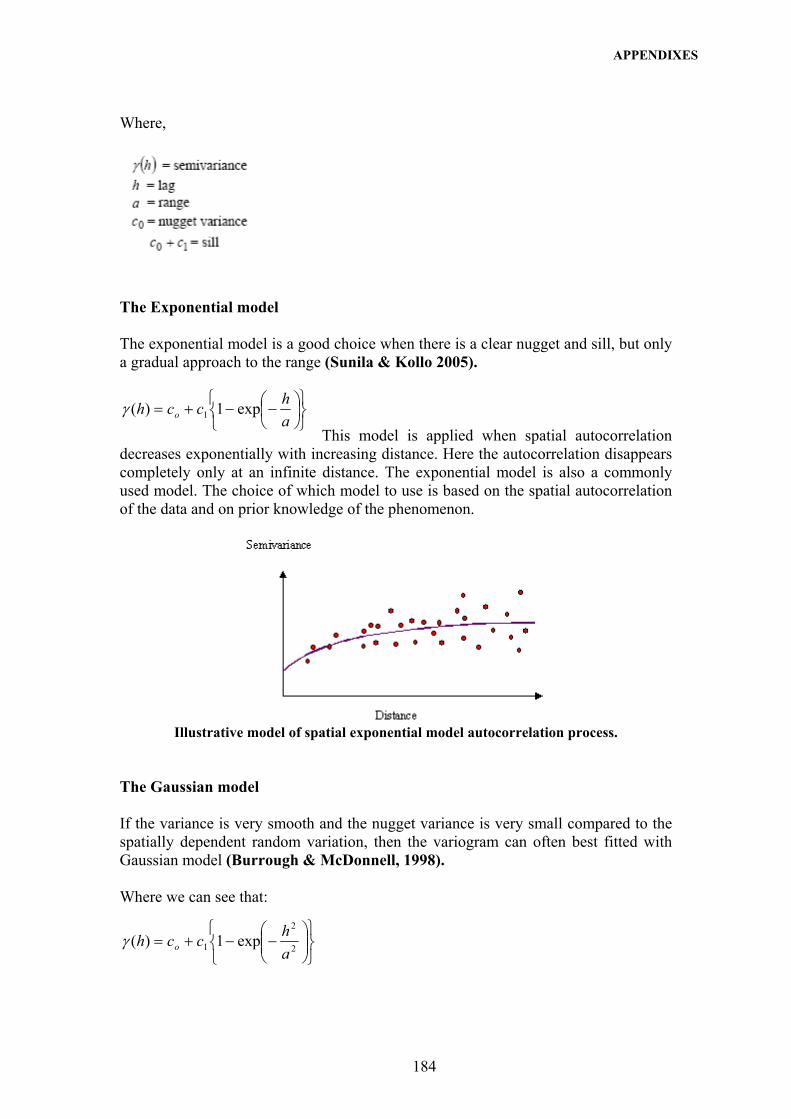
APPENDIXES
184
Where,
The Exponential model The exponential model is a good choice when there is a clear nugget and sill, but only a gradual approach to the range (Sunila & Kollo 2005).
This model is applied when spatial autocorrelation
decreases exponentially with increasing distance. Here the autocorrelation disappears completely only at an infinite distance. The exponential model is also a commonly used model. The choice of which model to use is based on the spatial autocorrelation of the data and on prior knowledge of the phenomenon.
Illustrative model of spatial exponential model autocorrelation process.
The Gaussian model If the variance is very smooth and the nugget variance is very small compared to the spatially dependent random variation, then the variogram can often best fitted with Gaussian model (Burrough & McDonnell, 1998). Where we can see that:
⎭⎬⎫
⎩⎨⎧
⎟⎠⎞
⎜⎝⎛−−+=
ahcch o exp1)( 1γ
⎭⎬⎫
⎩⎨⎧
⎟⎟⎠
⎞⎜⎜⎝
⎛−−+= 2
2
1 exp1)(ahcch oγ

APPENDIXES
185
Range, sill, and nugget As previously discussed, the semivariogram depicts the spatial autocorrelation of the measured sample points. Because of a basic principle of geography (things that are closer are more alike), measured points that are close will generally have a smaller difference squared than those farther apart. Once each pair of locations is plotted after being binned, a model is fit through them. Range, sill, and nugget are commonly used to describe these models. The distance where the model first flattens is known as the range. Sample locations separated by distances closer than the range are spatially autocorrelated, whereas locations farther apart than the range are not. The value at which the semivariogram model attains the range (the value on the y-axis) is called the sill. A partial sill is the sill minus the nugget (see the following section). Theoretically, the nugget value at zero separation distance (for example, lag = 0), the semivariogram value is zero. If for example the semivariogram model intercepts the y-axis at 2, then the nugget is 2.
Illustrative model of nugget, sill, & range relationship

APPENDIXES
186
Appendix 11 Validation and Modeling for Chloride
Appendix 11.1 Validation Trials and Results for Chloride in year 2001
Method Spline (RBF) Regularized Spline Spline with Tension
Parameter Optimized 0.016212 0.005019 Mean (ME): -17.03 -15.82
Root-Mean-Square (RMSE): 211.7 206.2 OK
Method IDW
Power 2 2 3.2273 3.2273 10 smooth (0-1) 0.5 1 0.5 1 1
Cross Validation statistics
Mean (ME): -21.53 -15.56 -11.16 -10.99 -8.231 Root-Mean-Square (RMSE): 196 194.2 187.6 187.5 205.7
OK
Method Kriging/Ordinary Geostatisitcal Method/Output Prediction Map
Transformation log
Semivariogram parameters Spherical Expo.
Partial sill 0.93551 0.93551 0.8442 1.0926 1.1225 0.88253 0.96802 0.84165
Nugget 0 0 0 0 0 0 0 0 Lag Size 774.81 774.81 1000 500 774.81 1000 500 1200 Smooth 0.5 1 1 1 0.5 1 1 1
Cross Validation statistics
Mean (ME): 6.613 1.936 -2.076 7.512 6.431 0.982 7.524 0.01636 Root-Mean-Square (RMSE): 214.4 194.6 193.5 198.7 204.8 195.8 195.8 195.7
OK

APPENDIXES
187
Appendix 11.2 Validation Trials and Results for Chloride in year 2003
Method Spline (RBF) Regularized Spline Spline with Tension
Parameter Optimized 0.019769 0.012102 Mean (ME): -8.972 -8.951
Root-Mean-Square (RMSE): 258.2 258.4
OK
Method IDW
Power 2 2 3.1965 3.1965 10 smooth (0-1) 0.5 1 0.5 1 1
Cross Validation statistics
Mean (ME): -27.91 -19.56 -31.01 -28.95 -33.98 Root-Mean-Square (RMSE): 251.7 253.6 245.7 245.9 264.4
OK
Method Kriging/Ordinary Geostatisitcal Method/Output Prediction Map
Transformation log
Semivariogram parameters Spherical Expo. Partial sill 1.036 1.036 0.8492 0.8325 1.1631 1.1631 0.8314 0.7554 0.7395
Nugget 0 0 0 0 0 0 0 0.0145 0.0430 Lag Size 635.36 635.36 1000 1500 635.36 635.36 1500 2300 2400 Smooth 0.5 1 0.5 1 0.5 1 1 1 1
Cross Validation statistics
Mean (ME): 10.11 13.56 8.093 7.261 17.4 17.84 11.93 8.164 11.13 Root-Mean-Square (RMSE): 266.2 268.6 269.1 267.7 264.6 264.2 260.9 259 257.1
OK

APPENDIXES
188
Appendix 11.3 Validation Trials and Results for Chloride in year 2005
Method Spline (RBF) Regularized Spline Spline with Tension
Parameter Optimized 0.0056453 0.001735 Mean (ME): -27.17 -30.44
Root-Mean-Square (RMSE): 340.1 333.4
OK
Method IDW
Power 2 2 10 1 smooth (0-1) 0.5 1 1 1
Cross Validation statistics
Mean (ME): -50.01 -44.32 -63.04 -17.58 Root-Mean-Square (RMSE): 349.5 358.6 364.9 406.1
OK
Method Kriging/Ordinary Geostatisitcal Method/Output Prediction Map
Transformation log
Semivariogram parameters Spherical Expo. Partial sill 0.94891 1.1934 0.95041 0.91038 0.99974 1.1631 0.92099 1.1366
Nugget 0.033329 0.057465 0 0.009812 0 0 0 0 Lag Size 983.43 500 1500 1200 983.43 635.36 1200 500 Smooth 0.5 1 1 1 0.5 1 1 1
Cross Validation statistics
Mean (ME): -10.28 4.655 -10.31 -8.78 3.237 4.796 3.864 12.02 Root-Mean-Square (RMSE): 332.2 332.8 333.8 332.4 336.7 337 338.9 336.6
OK

APPENDIXES
189
Appendix 11.4 Validation Trials and Results for Chloride in year 2007
Method Spline (RBF)
Regularized Spline Spline with Tension
Parameter Optimized 1.0696 1.5406 Mean (ME): -16.84 -17.26
Root-Mean-Square (RMSE): 505.4 505
OK
Method IDW
Power 2 2 2.6853 2.3946 2.3946 10 smooth (0-1) 0.5 1 0.5 0.5 1 1
Cross Validation statistics
Mean (ME): -26.17 -26.91 -42.73 -36.97 -37.35 -67.47 Root-Mean-Square (RMSE): 514.3 513.9 510.5 511.1 511 555.1
OK
Method Kriging/Ordinary Geostatisitcal Method/Output Prediction Map
Transformation log
Semivariogram parameters Spherical Expo. Partial sill 0.85736 0.85736 0.97391 0.77707 0.99424 0.88696 1.1055
Nugget 0.11035 0.11035 0.12336 0.10771 0 0 0.01933 Lag Size 746.65 746.65 500 1000 746.65 1000 500 Smooth 0.5 1 1 1 0.5 1 1
Cross Validation statistics
Mean (ME): -9.362 -3.944 0.8896 -13.22 -7.787 -6.427 0.8638 Root-Mean-Square (RMSE): 473.1 474.3 474.5 471 489.5 492.2 485.6
OK

APPENDIXES
190
Appendix 12 Validation and Modeling for Water Level
Appendix 12.1 Validation Trials and Results for Water Level in year 2001
Method Spline (RBF)
Regularized Spline Spline with Tension
Parameter Optimized 0.018213 0.004366 Mean (ME): -0.000608 0.008238
Root-Mean-Square (RMSE): 1.293 1.2
OK
Method IDW
Power 2 2 10 2.3103 2.5008 2.5306 smooth (0-1) 0.5 1 0.5 0.5 1 0.8
Cross Validation statistics
Mean (ME): 0.0100 0.0099 0.0743 0.0222 0.0325 0.0327 Root-Mean-Square (RMSE): 1.243 1.267 1.534 1.222 1.221 1.219
OK
Method Kriging/Ordinary Geostatisitcal Method/Output Prediction Map
Transformation None
Semivariogram parameters Spherical Expo. Partial sill 8.6411 8.6411 6.0051 7.9131 9.5694 9.5694 6.5553 3.8288
Nugget 1.8618 1.8618 0.066472 2.1801 0.52827 0.52827 0 0 Lag Size 2695.7 2695.7 2000 3000 2695.7 2695.7 1000 500 Smooth 0.5 1 0.5 0.5 1 0.5 1 1
Cross Validation statistics
Mean (ME): 0.001763 0.007969 0.04789 -0.00275 0.03106 0.02917 0.02901 0.01743 Root-Mean-Square (RMSE): 1.426 1.418 1.282 1.459 1.266 1.282 1.167 1.116
OK

APPENDIXES
191
Appendix 12.2 Validation Trials and Results for Water Level in year 2003
Method Spline (RBF)
Regularized Spline Spline with Tension
Parameter Optimized 0.031901 0.007482 Mean (ME): -0.005668 0.006603
Root-Mean-Square (RMSE): 1.53 1.444
OK
Method IDW
Power 2 2 2.4874 2.4874 10 smooth (0-1) 0.5 1 0.5 1 1
Cross Validation statistics
Mean (ME): 0.000874 0.001147 0.01483 0.01618 -0.01239 Root-Mean-Square (RMSE): 1.423 1.417 1.362 1.37 1.732
OK
Method Kriging/Ordinary Geostatisitcal Method/Output Prediction Map
Transformation None
Semivariogram parameters Spherical Expo. Partial sill 7.9273 7.9273 7.3337 7.8863 9.7464 9.7464 9.7039 9.7362
Nugget 0 0 0 0 0 0 0 0 Lag Size 2628.5 2628.5 2000 2500 2628.5 2628.5 2500 3000 Smooth 0.5 1 0.5 1 0.5 1 1 1
Cross Validation statistics
Mean (ME): 0.04171 0.03238 0.03655 0.03229 0.02894 0.02501 0.02497 0.02502 Root-Mean-Square (RMSE): 1.479 1.464 1.486 1.463 1.443 1.422 1.421 1.422
OK

APPENDIXES
192
Appendix 12.3 Validation Trials and Results for Water Level in year 2005
Method Spline (RBF)
Regularized Spline Spline with Tension
Parameter Optimized 30.661 0.51753 Mean (ME): 0.003301 0.1222
Root-Mean-Square (RMSE): 1.778 1.677
OK
Method IDW
Power 2 2 2.8772 2.8772 10 smooth (0-1) 0.5 1 0.5 1 1
Cross Validation statistics
Mean (ME): 0.02121 0.001312 0.05608 0.05502 0.03546 Root-Mean-Square (RMSE): 1.414 1.499 1.35 1.372 1.569
OK
Method Kriging/Ordinary Geostatisitcal Method/Output Prediction Map
Transformation None
Semivariogram parameters Spherical Expo. Partial sill 10.505 10.505 7.963 8.6882 11.263 11.263 8.471 7.1874
Nugget 2.4871 2.4871 0 0 0 0 0 0 Lag Size 2748 2748 2000 750 2748 2748 2000 750 Smooth 0.5 1 1 1 0.5 1 1 1
Cross Validation statistics
Mean (ME): -0.004681 -0.003879 0.03001 0.0134 0.04238 0.02455 0.01679 0.007288 Root-Mean-Square (RMSE): 1.519 1.517 1.104 1.067 1.133 1.113 1.077 1.064
OK

APPENDIXES
193
Appendix 12.4 Validation Trials and Results for Water Level in year 2007
Method Spline (RBF)
Regularized Spline Spline with Tension
Parameter Optimized 24.823 0.29112 Mean (ME): -0.1475 0.03052
Root-Mean-Square (RMSE): 2.369 2.218
OK
Method IDW
Power 2 2 2.6643 2.6643 10 smooth (0-1) 0.5 1 1 0.5 1
Cross Validation statistics
Mean (ME): -0.1474 -0.1209 -0.1036 -0.1032 -0.1732 Root-Mean-Square (RMSE): 1.898 1.926 1.852 1.848 2.06
OK
Method Kriging/Ordinary Geostatisitcal Method/Output Prediction Map
Transformation None
Semivariogram parameters Spherical Expo. Partial sill 12.267 12.267 10.62 10.707 13.7 13.7 11.27 10.707
Nugget 3.8724 3.8724 0 0 0 0 0 0 Lag Size 2748 2748 2000 1600 2748 2748 2000 1600 Smooth 0.5 1 1 1 0.5 1 1 0.5
Cross Validation statistics
Mean (ME): -0.02023 -0.06515 -0.08456 -0.08758 -0.06127 -0.08617 -0.06432 -0.06504 Root-Mean-Square (RMSE): 2.083 2.108 1.577 1.535 1.61 1.594 1.557 1.542
OK

APPENDIXES
194
Appendix 13 Validation and Modeling for Rainfall
Appendix 13.1 Validation Trials and Results for Rainfall in year 2001
Method Spline (RBF)
Regularized Spline Spline with Tension
Parameter Optimized 0.0004537 0.000193 Mean (ME): 7.087 5.274
Root-Mean-Square (RMSE): 44.1 36.6
OK
Method IDW
Power 2 2 6.7128 6.7128 10 smooth (0-1) 0.5 1 0.5 1 0.5
Cross Validation statistics
Mean (ME): 16.01 9.83 9.308 9.21 9.2230 Root-Mean-Square (RMSE): 60.3 38.23 39.46 39.31 40.91
OK
Method Kriging/Ordinary Geostatisitcal Method/Output Prediction Map
Transformation log
Semivariogram parameters Spherical Expo. Partial sill 0.038164 0.038164 0.027514 0.014292 0.034475 0.013191 0.01137 0.007833
Nugget 0 0 0 0 0 0 0 0 Lag Size 2695 2695 2000 1500 2695.7 1500 1200 1000 Smooth 0.5 1 0.5 1 0.5 1 0.5 1
Cross Validation statistics
Mean (ME): 5.289 8.584 5.513 7.078 7.102 7.507 7.45 7.143 Root-Mean-Square (RMSE): 38.19 33.83 40.44 33.45 51.89 34.05 34.24 34.68
OK

APPENDIXES
195
Appendix 13.2 Validation Trials and Results for Rainfall in year 2003
Method Spline (RBF)
Regularized Spline Spline with Tension
Parameter Optimized 0.0004462 1.35E-05 Mean (ME): 0.103 -14.41
Root-Mean-Square (RMSE): 111 102.1
OK
Method IDW
Power 2 2 5.1879 5.1879 10 smooth (0-1) 0.5 1 0.5 1 0.5
Cross Validation statistics
Mean (ME): 16.88 -5.38 -20.88 -23.83 -32.54 Root-Mean-Square (RMSE): 131.8 105.6 106 105.5 111.6
OK
Method Kriging/Ordinary Geostatisitcal Method/Output Prediction Map
Transformation log
Semivariogram parameters Spherical Expo. Partial sill 0.19871 0.19871 0.1313 0.2352 0.17708 0.17708 0.1183 0.2089
Nugget 0 0 0 0 0 0 0 0 Lag Size 2695 2695 2000 3000 2695 2695 2000 3000 Smooth 0.5 1 0.5 1 0.5 1 1 1
Cross Validation statistics
Mean (ME): -1.723 -1.359 -4.254 0.521 2.339 2.377 -1.094 4.295 Root-Mean-Square (RMSE): 104 102.2 103.4 101.9 103.3 101.9 102.6 101.9
OK

APPENDIXES
196
Appendix 13.3 Validation Trials and Results for Rainfall in year 2005
Method Spline (RBF)
Regularized Spline Spline with Tension
Parameter Optimized 0.0030383 0.004376 Mean (ME): -1.849 -1.607
Root-Mean-Square (RMSE): 29.720 29.4
OK
Method IDW
Power 2 2 1 1 10 smooth (0-1) 0.5 1 0.5 1 0.5
Cross Validation statistics
Mean (ME): -5.628 -4.097 -3.43 -3.19 -32.54 Root-Mean-Square (RMSE): 31.24 33.77 32.51 32.13 111.6
OK
Method Kriging/Ordinary Geostatisitcal Method/Output Prediction Map
Transformation log
Semivariogram parameters Spherical Expo. Partial sill 0.00561 0.00561 0.004739 0.005338 0.007021 0.007021 0.005701 0.00749
Nugget 0.0041087 0.0041087 0.004612 0.00424 0.002833 0.002833 0.003641 0.002128 Lag Size 2695 2695 3000 2000 2695 2695 3000 2000 Smooth 0.5 1 1 1 0.5 1 1 1
Cross Validation statistics
Mean (ME): -1.442 -2.314 -2.301 -2.313 -0.6931 -2.542 -2.498 -2.631 Root-Mean-Square (RMSE): 29.1 33.02 32.82 32.96 29.02 32.71 32.49 32.69
OK

APPENDIXES
197
Appendix 13.4 Validation Trials and Results for Rainfall in year 2007
Method Spline (RBF)
Regularized Spline Spline with Tension
Parameter Optimized 0.0017835 0.001022 Mean (ME): 7.021 6.995
Root-Mean-Square (RMSE): 71.91 70.67
OK
Method IDW
Power 2 2 7.7733 7.7733 10 smooth (0-1) 0.5 1 0.5 1 0.5
Cross Validation statistics
Mean (ME): 20.22 10.15 9.789 9.817 9.432 Root-Mean-Square (RMSE): 68.67 50.76 50.03 50.33 50.91
OK
Method Kriging/Ordinary
Geostatisitcal Method/Output Prediction Map Transformation log
Semivariogram parameters Spherical Expo.
Partial sill 0.09088 0.09088 0.004739 0.00533 0.08149 0.08149 0.1008 0.05178 Nugget 0 0 0.004612 0.0042 0 0 0 0
Lag Size 2695 2695 3000 2000 2695 2695 3000 2000 Smooth 0.5 1 0.5 1 0.5 1 1 1
Cross Validation statistics
Mean (ME): 0.8529 8.197 -2.201 -2.313 3.574 9.053 10.25 7.219 Root-Mean-Square (RMSE): 56.51 57.71 58.18 62.96 61.94 51.53 51.89 51.03
OK