Embed Size (px)
Citation preview

ASSESSMENT OF PERMEABILITY FROM WELL LOGS BASED ON CORE CALIBRATION AND SIMULATION OF MUD-FILTRATE
INVASION Jesús M. Salazar, Carlos Torres-Verdín, The University of Texas at Austin, and Richard
Sigal*, Anadarko Petroleum Corporation
Abstract
This paper describes the application of a new methodology to estimate permeability
of clastic rock formations based on the numerical simulation of the physics of mud-
filtrate invasion. The methodology assumes a key well with a complete suite of well logs
and rock-core laboratory measurements of porosity, permeability, capillary pressure, and
relative permeability. For additional wells in the same field, absolute permeability is
estimated by matching the shallow resistivity measurements with the electrical resistivity
in the flushed zone yielded by the simulation of mud-filtrate invasion. We describe the
application of this methodology to the estimation of permeability in three wells
penetrating the same over-pressured tight-gas sands of the East Texas Bossier formation.
Conventional rock-core porosity and permeability measurements, along with
capillary pressure, are used to determine rock types and flow units in the cored key well.
Estimates of permeability based on a modified version of Winland’s equation agree with
the measured permeability of the available rock-core samples. Simulations of mud-filtrate
invasion account for the dynamic process of immiscible flow between mud-filtrate and
in-situ gas as well as for salt mixing between mud-filtrate and connate water. Moreover,
the simulations properly reproduce the effect of mudcake buildup along the borehole
wall. Two-dimensional spatial distributions of water saturation and salt concentration
* Currently with University of Oklahoma
1
obtained from the simulations are used to calculate spatial distributions of electrical
resistivity. The latter are checked against the measured shallow, medium, and deep
resistivity logs to calibrate time of invasion and Archie’s saturation and cementation
exponents.
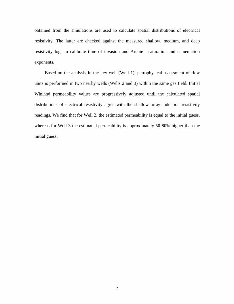
Based on the analysis in the key well (Well 1), petrophysical assessment of flow
units is performed in two nearby wells (Wells 2 and 3) within the same gas field. Initial
Winland permeability values are progressively adjusted until the calculated spatial
distributions of electrical resistivity agree with the shallow array induction resistivity
readings. We find that for Well 2, the estimated permeability is equal to the initial guess,
whereas for Well 3 the estimated permeability is approximately 50-80% higher than the
initial guess.
2
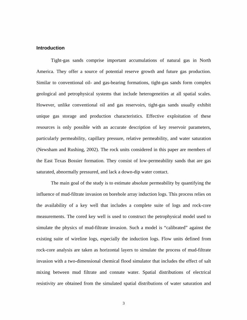
Introduction
Tight-gas sands comprise important accumulations of natural gas in North
America. They offer a source of potential reserve growth and future gas production.
Similar to conventional oil- and gas-bearing formations, tight-gas sands form complex
geological and petrophysical systems that include heterogeneities at all spatial scales.
However, unlike conventional oil and gas reservoirs, tight-gas sands usually exhibit
unique gas storage and production characteristics. Effective exploitation of these
resources is only possible with an accurate description of key reservoir parameters,
particularly permeability, capillary pressure, relative permeability, and water saturation
(Newsham and Rushing, 2002). The rock units considered in this paper are members of
the East Texas Bossier formation. They consist of low-permeability sands that are gas
saturated, abnormally pressured, and lack a down-dip water contact.
The main goal of the study is to estimate absolute permeability by quantifying the
influence of mud-filtrate invasion on borehole array induction logs. This process relies on
the availability of a key well that includes a complete suite of logs and rock-core
measurements. The cored key well is used to construct the petrophysical model used to
simulate the physics of mud-filtrate invasion. Such a model is “calibrated” against the
existing suite of wireline logs, especially the induction logs. Flow units defined from
rock-core analysis are taken as horizontal layers to simulate the process of mud-filtrate
invasion with a two-dimensional chemical flood simulator that includes the effect of salt
mixing between mud filtrate and connate water. Spatial distributions of electrical
resistivity are obtained from the simulated spatial distributions of water saturation and
3

salt concentration using Archie’s law. Matching the simulated flushed-zone resistivity
with the measured shallow resistivity logs provides a direct assessment of Archie’s
parameters, m and n, for a given rock type.
The first stage of the study consists of defining rock types by relating geological
framework, lithofacies, and petrology to porosity, permeability, and capillary pressure.
Rock types represent reservoir units with a distinct porosity-permeability relationship and
a unique water saturation range for a given height above the free water level. The second
stage of the work integrates the rock type model with formation evaluation data to define
reservoir compartments and flow units. Log and rock-core measurements are integrated
to extend the rock-type model, and to compute continuous storage and flow capacity
specific to a given flow unit.
The third stage of the work quantifies the influence of mud-filtrate invasion on the
spatial distribution of fluids in permeable rocks around the wellbore. Fresh water-based
mud was used to drill the key well. High overbalance pressure and low porosity of the
rock combine to cause relatively deep invasion of mud-filtrate (Wu et al, 2004 and
George et al, 2004). Gas saturation of the formation ranges from 85 to 98% showing, in
general, low or sometimes null values of irreducible water saturation that are consistent
with NMR and capillary pressure measurements. Salinity of mud filtrate is about 30
kppm for the key well whereas salinity of connate water ranges between 200 and 220
kppm. We perform a sensitivity analysis of the time evolution of mud-filtrate invasion.
After one day of invasion, spatial distributions of electrical resistivity are calculated from
the simulated spatial distributions of water saturation and salt concentration.
4

Subsequently, shallow resistivity (Rxo) values are computed and compared to the shallow
array induction measurements.
Based on the analysis for the key well, a petrophysical assessment is performed in
two additional wells in the same field. These two additional wells include a basic suite of
logs but lack rock-core measurements. Simulations of mud-filtrate invasion are carried
out in each well with the only free parameter being average absolute permeability per
flow unit. All of the remaining petrophysical parameters required by the simulation of
invasion are either estimated from well logs or extrapolated from the key well. A
modified Winland permeability equation (Pittman, 1992) is used to compute the initial
value of absolute permeability. This initial permeability is progressively adjusted in the
simulation of mud-filtrate invasion until an acceptable match is obtained between the
calculated shallow formation resistivity and the shallow-reading array induction log.
Such a technique embodies a new methodology to estimate in-situ absolute permeability
that is consistent with the radial length of investigation and vertical resolution of
induction logs.
Depositional System and Rock Typing
The Bossier Formation consists of marine shale deposits and localized sand units
(Williams et al, 2001). There are two fairway systems in the upper member of Bossier: a
shelf edge, stacked deltaic fairway, and a relatively deeper water fan fairway that
originates from a combination of sea level fall and climate change (Klein and Chaivre,
2002). The gas field considered in this paper comprises large sand-rich shorelines within
the Bossier Formation (Klein and Chaivre, 2002). This causes a relatively high degree of
lateral continuity of the clean sand bodies observed across the field. Sedimentological
5
description of rock-core samples indicates presence of different litho-facies. Rocks
consist of fine to very fine grained clean sandstones, slightly shaly to shaly sandstones,
calcite-cemented sandstones, and shaly/sandy limestones to calcareous dolostones.
Diagenetic effects on sandstones include an increase of tortuosity and a reduction of the
pore throat size. A decrease of porosity and permeability is the usual way in which the
rock displays the influence of diagenesis. Mechanical compaction, quartz overgrowth
(thereby inducing cementation), grain coating/pore lining clay development, and grain
dissolution are the most common forms of diagenetic overprint in these rocks (Newsham
and Rushing, 2002).
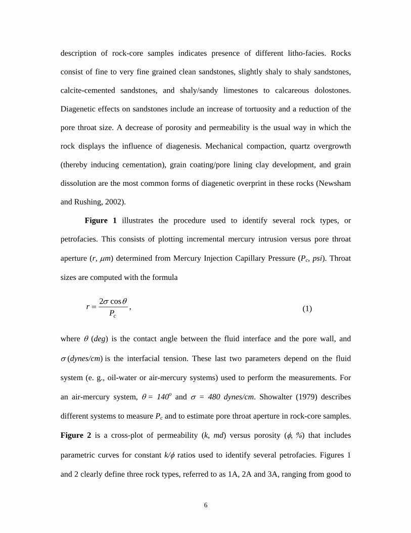
Figure 1 illustrates the procedure used to identify several rock types, or
petrofacies. This consists of plotting incremental mercury intrusion versus pore throat
aperture (r, μm) determined from Mercury Injection Capillary Pressure (Pc, psi). Throat
sizes are computed with the formula
,cos2
cPr θσ
= (1)
where θ (deg) is the contact angle between the fluid interface and the pore wall, and
σ (dynes/cm) is the interfacial tension. These last two parameters depend on the fluid
system (e. g., oil-water or air-mercury systems) used to perform the measurements. For
an air-mercury system, θ = 140o and σ = 480 dynes/cm. Showalter (1979) describes
different systems to measure Pc and to estimate pore throat aperture in rock-core samples.
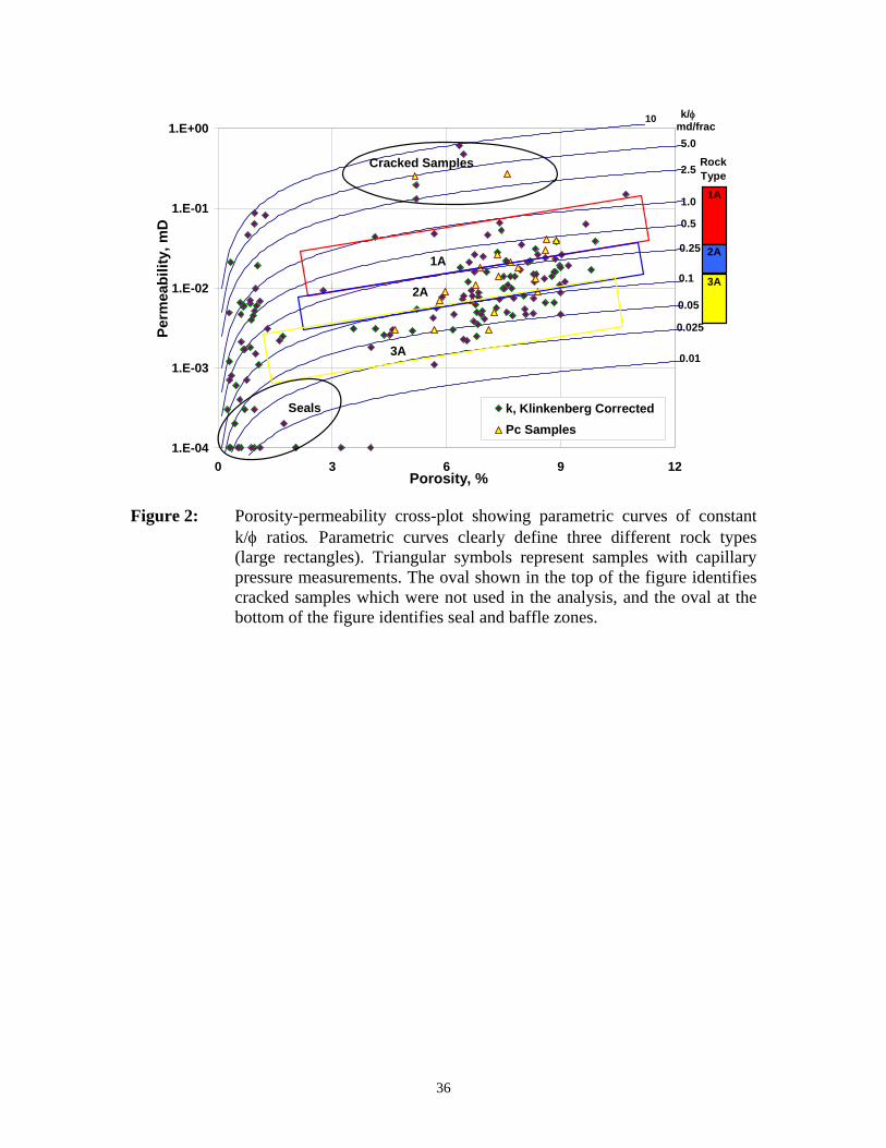
Figure 2 is a cross-plot of permeability (k, md) versus porosity (φ, %) that includes
parametric curves for constant k/φ ratios used to identify several petrofacies. Figures 1
and 2 clearly define three rock types, referred to as 1A, 2A and 3A, ranging from good to
6

poor quality, respectively. Table 1 describes values of porosity, permeability, pore throat
aperture size, and k/φ ratio for each rock type. Effective porosity varies from 1 to 11 %
while absolute permeability ranges from 0.001 to 0.2 md. The permeability of non-
reservoir and seal rocks is lower than 0.001 md. Similar to most tight-gas sands, the
formation under analysis exhibits stress-dependent permeability and, to a less extent,
stress-dependent porosity. In particular, the sensitivity of absolute permeability to in-situ
stress is significant. The analysis described in this paper is carried out using routine rock-
core porosity and Klinkenberg-corrected absolute permeability measurements at an
overburden pressure of 2500 psi.
As shown in Figure 3, capillary pressure curves also distinctly discriminate the
various petrofacies. The lowest quality rock type, 3A, displays very low values of
porosity and permeability. By observing the shape of capillary pressure curves, it is
possible to infer that 3A-type rocks play the role of vertical flow barriers or seals. They
are therefore considered non-reservoir rocks. Figure 4 shows that the Transverse
Relaxation Time (T2) spectrum reconstructed from the 100% brine-saturated NMR
measurements is in agreement with the analysis described above. Rock 1A exhibits a
dominant T2 higher than 90 ms, 2A between 30 ms and 90 ms, and for rock 3A T2 is less
than 30 ms.
Petrophysical Assessment of Flow Units
We define several flow units penetrated by the key well in order to upscale the
geological and petrophysical description for input to the numerical simulation of mud-
filtrate invasion. A Stratigraphic Modified Lorenz Plot (SMLP) of percent of cumulative
flow capacity (%kh) versus percent of cumulative storage capacity (%φh) is constructed
7
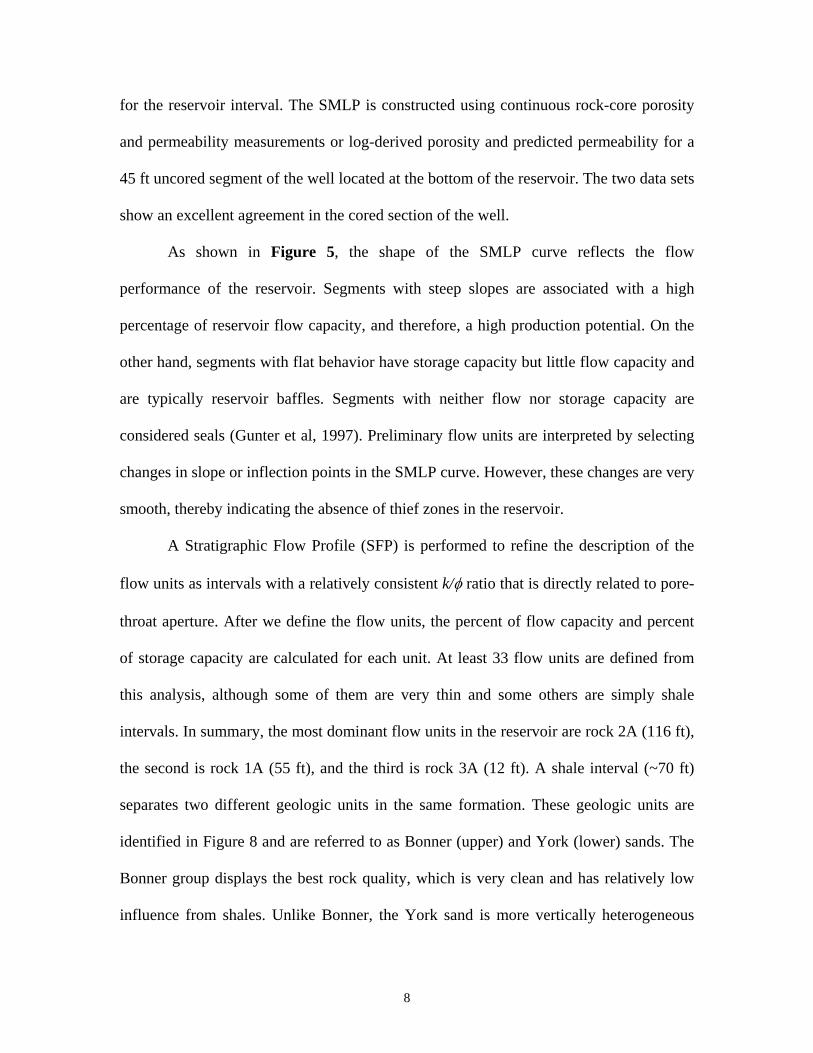
for the reservoir interval. The SMLP is constructed using continuous rock-core porosity
and permeability measurements or log-derived porosity and predicted permeability for a
45 ft uncored segment of the well located at the bottom of the reservoir. The two data sets
show an excellent agreement in the cored section of the well.
As shown in Figure 5, the shape of the SMLP curve reflects the flow
performance of the reservoir. Segments with steep slopes are associated with a high
percentage of reservoir flow capacity, and therefore, a high production potential. On the
other hand, segments with flat behavior have storage capacity but little flow capacity and
are typically reservoir baffles. Segments with neither flow nor storage capacity are
considered seals (Gunter et al, 1997). Preliminary flow units are interpreted by selecting
changes in slope or inflection points in the SMLP curve. However, these changes are very
smooth, thereby indicating the absence of thief zones in the reservoir.
A Stratigraphic Flow Profile (SFP) is performed to refine the description of the
flow units as intervals with a relatively consistent k/φ ratio that is directly related to pore-
throat aperture. After we define the flow units, the percent of flow capacity and percent
of storage capacity are calculated for each unit. At least 33 flow units are defined from
this analysis, although some of them are very thin and some others are simply shale
intervals. In summary, the most dominant flow units in the reservoir are rock 2A (116 ft),
the second is rock 1A (55 ft), and the third is rock 3A (12 ft). A shale interval (~70 ft)
separates two different geologic units in the same formation. These geologic units are
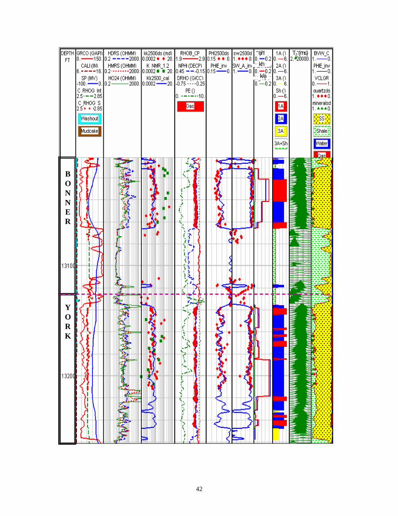
identified in Figure 8 and are referred to as Bonner (upper) and York (lower) sands. The
Bonner group displays the best rock quality, which is very clean and has relatively low
influence from shales. Unlike Bonner, the York sand is more vertically heterogeneous
8

due to variations of grain size and grain sorting that cause substantial variations of
permeability.
Log-Computed Effective Porosity and Water Saturation
The salinity of connate water is over 200 kppm (Newsham and Rushing, 2002).
Therefore, due to this relatively high salt concentration Archie’s equation can be used to
accurately compute water saturation (Sw) without corrections for the presence of clay.
Accordingly, water saturation is given by
wnw mt
R aS
Rφ= , (2)
where φ is effective porosity, Rw is connate water resistivity, Rt is true formation
resistivity, a is the tortuosity factor, and m and n are the cementation and saturation
exponents, respectively.
At the outset, both cementation and saturation exponents are assumed equal to 2,
while the tortuosity factor, a is taken as 1 in equation (2). However, in a subsequent
section of this paper we introduce a method to refine the estimates of m and n.
Commutation analysis and fluid inclusion microthermometry was used to
calculate connate water salinity from preserved core samples in the Bossier Formation
(Newsham and Rushing, 2002). In turn, connate water resistivity at reservoir conditions
is calculated using the calculated salinity of 220 kppm. This yields a value of Rw equal to
0.0126 ohm.m at reservoir conditions and of 0.045 ohm.m at 75 oF (Newsham and
Rushing, 2002). The effective porosity is calculated using a dual-fluid dual-mineral non-
linear model. Accordingly, a Newton-Raphson method is used to solve the equation
9

( ) ( )1 2 2 1 ,wnb smt
R aV V
Rρ φ ρ ρ ρ φ ρ ρ
φ
⎡ ⎤= − + + − − +⎢ ⎥
⎢ ⎥⎣ ⎦h ma sh sh
(3)
for φ, where ρb is the measured bulk density, and ρma is the matrix density obtained from
rock-core measurements. Matrix densities range from 2.64 g/cm3 to 2.67 g/cm3 in the
reservoir rock but never exceed 2.68 g/cm3. The remaining densities are as follows: shale,
ρsh = 2.68 g/cm3, water, ρ1 ≈ 1.0 g/cm3, and gas-mud-filtrate mixture, ρ2 ≈ 0.80 g/cm3.
Volumes of shale concentration, Vsh, are obtained with a linear transformation of gamma-
ray readings. Thomas and Stieber (1975) methodology is applied to rock-core
measurements in order to diagnose the type of shale distribution across the formation. In
so doing, we remark that most of the available core plugs subject to special rock-core
analyses were taken in relatively clean sand intervals. Figure 6 shows a Thomas-Stieber
diagram indicating that dispersed shale is the dominant type of shale distribution in the
formation under study. Figure 8 shows that X-ray diffraction (XRD) mineralogy
measurements agree well with the computed shale concentration. The same figure
compares the log-calculated effective porosity with the measured rock-core porosity at
2500 psi confining pressure. Rock-core porosity and log-calculated porosity exhibit
similar trends. Deep induction resistivity readings, HDRS†, are assumed as the true
formation resistivity in the virgin zone. The application of Archie’s equation provided
ranges of water saturation for each previously defined rock type. It was found that water
saturation for rock type 1A ranges from 2 to 12%, rock 2A from 12 to 30%, and rock 3A
is higher than 30%. Dean-Stark tracer-corrected water saturation measurements were
available for 242 rock-core samples. Such water saturation measurements are shown in
† Mark of Halliburton
10

Figure 8 along with log-calculated values of water saturation obtained via Archie’s
equation.
Absolute Permeability
The porosity and permeability of selected rock-core samples were measured over
a wide range of values of in-situ stress. A slight reduction of porosity is observed with an
increase of in-situ stress. On the other hand, permeability strongly decreases as stress
increases. The dependency of both porosity and permeability on in-situ stress is more
pronounced for the lower quality rock types. A permeability relationship that matches
rock-core measurements is therefore difficult to infer due to such stress-dependence.
Various techniques were unsuccessfully employed to approach such a problem, including
Tixier, Wyllie and Rose, Coates (Balan et al, 1995), and Winland’s R35 method (Pittman,
1992). We applied Winland’s method to estimate permeability from log data.
Accordingly, a multilinear regression model was used with one dependent variable, k
(md), and two independent variables, r (μm) and φ (%), viz.,
,dcrbk φ⋅= (4)
where b, c, and d are scaling constants. The pore throat aperture is calculated from
equation (1) using the pressure readings at the point where the mercury injection
saturation is around 35%. This saturation approximately coincides with the maximum
mercury injection rate (Pittman, 1992), and corresponds to the maximum of each curve in
Figure 1. Finally, we find an equation to estimate the Klinkenberg-corrected permeability
as a function of pore throat aperture and effective porosity at a confining pressure of 2500
psi, given by
11
0.858 1.930.0012k r φ= ⋅ . (5)
The correlation coefficient when using the above formula is 75%. Equation (5) is
different for air-uncorrected k, as well as for a net confining pressure of 800 psi. We
estimate pore throat aperture as a function of water saturation. Figure 7 is a cross-plot of r
vs. Sw together with the corresponding least-squares regression line (correlation
coefficient equal to 94%). Log-calculated values of water saturation are used to estimate
pore aperture based on the equation
0.93230.41 10 wSr −= × . (6)
The permeability track in Figure 8 indicates a good agreement between estimated
and rock-core permeability. Some scattered points are due either to measurements
performed on cracked samples or else to samples close to thin shale layers. Figure 8 also
shows permeability values estimated from NMR data. Clearly, equation (5) provides a
better match with the Klinkenberg-corrected permeability than with the NMR-base
permeability.
Numerical Simulation of Mud-Filtrate Invasion
Mud-filtrate invasion is a phenomenon that takes place in permeable porous media during
the drilling process due to mechanical overbalance and mud circulation. The radial length
of invasion is the radial distance that mud filtrate penetrates into the formation. This
distance depends on mud density, mud chemical composition, mud circulation pressure,
and time of filtration. Rock properties also play an important role in controlling the time
evolution of the invasion process (Wu et al, 2004). The rate of invasion of mud filtrate
into permeable rock formations depends on the filtrate viscosity, the solid content, and
12

the rheology constants of the mud (Wu et al, 2004). Such rate is computed as a flow rate
function resulting from mudcake buildup (George et al., 2004). The flow rate across the
mudcake is described by Darcy’s law, namely,
mcf
mcf
k A PQhμΔ
= , (7)
where Qf is the flow rate of mud filtrate across the borehole wall, kmc is the permeability
of mudcake, A is the cross-sectional area, μf is the viscosity of filtrate, hmc is the thickness
of mudcake, and ΔP is the pressure drop across mudcake.
In this paper, the process of mud-filtrate invasion is simulated in like manner to a
water injection process. Two-phase immiscible fluid flow is assumed in the numerical
simulation of invasion (George et al, 2004) using a modified version of a multi-phase
fluid flow chemical simulator. The original simulator was developed by The University
of Texas at Austin and is known as UTCHEM (Delshad et al, 1996). As in the case of
UTCHEM, the modified simulator is based on finite differences, and is here referred to as
INVADE. It was developed to solve the partial differential equations and boundary
conditions for immiscible radial flow coupled with mudcake growth. Either water-wet or
oil-wet systems can be simulated with INVADE. The development of the equations
assumes local thermodynamic equilibrium, Darcy’s law, ideal mixing, molecular
diffusion, and hydrodynamic dispersion (Delshad et al, 1996). Simulation of the process
of mud-filtrate invasion indicates that the flow rate of mud filtrate across mudcake
monotonically decreases as a function of time. After a short period of time (0.01 hours
for the case under consideration) this flow rate reaches a steady-state value specific to a
particular layer. A comprehensive explanation of the equations used by INVADE as well
13
as the required fluid and rock properties is given by Delshad et al (1996), Proett et al.
(2001), Wu et al. (2004), and George et al. (2004).
Simulation of Mud-Filtrate Invasion in the Key Well
Simulation of the process of mud-filtrate invasion is first performed in the key
well (Well 1). We make the assumption of cylindrical flow and permeability isotropy.
Each flow unit is represented with a material layer with its own effective porosity,
absolute permeability, and irreducible water saturation. Rock properties are considered
spatially invariant radially away from the wellbore. Reservoir flow units are
predominantly type 1A or 2A. Flow units are divided into several numerical layers
whenever necessary to improve the accuracy of the simulation. The radial grid consists of
61 logarithmically distributed nodes. Logarithmically spaced nodes provide adequate
spatial resolution for the time evolution of mud-filtrate invasion near the wellbore.
Figure 9 describes both the flow units and the finite-difference grid used in the
simulations of mud-filtrate invasion. UTCHEM requires that relative permeability and
capillary pressure curves be expressed in terms of Brooks-Corey parameters (Corey,
1994). Laboratory data are used to estimate the parameters included in the Corey-type
capillary pressure (Corey, 1994) and relative permeability curves (Corey, 1994, and
Lake, 1989). Table 2 is a summary of the parameters used in Corey’s equations for
capillary pressure, ep, and Pco, and for relative permeability, ew, enw, and relative
permeability end points (krio). Appendix A briefly describes the physical meaning of the
parameters included in the Brooks-Corey equations.
In the invasion process, mud filtrate advances from the borehole wall toward the
formation while mixing with connate water. As a result, salt concentration will vary
14
radially from mud-filtrate salinity at the wellbore to connate water salinity in the
uninvaded zone (virgin zone).
Two-dimensional spatial distributions of water saturation and salt concentration
are output by the numerical simulation of mud-filtrate invasion. Values of salt
concentration are converted to equivalent values of water resistivity (Rw) using the
Dresser Atlas equation (Bigelow, 1992)
[ ]0.9553647.5 81.770.0123
6.77wRTNaCl
⎛ ⎞⎛ ⎞⎜ ⎟= + ⎜⎜ ⎟ +⎝⎝ ⎠⎟⎠
, (8)
where T is reservoir temperature in oF, and [NaCl] is salt concentration in ppm. The
corresponding value of the rock’s electrical resistivity, Rt, is calculated with equation (2).
A detailed sensitivity analysis is performed to assess the effect of invasion time
on the simulated spatial distributions of electrical resistivity. This analysis considers both
Bonner and York sands divided into 10 and 20 layers, respectively. Impermeable shale
beds bound the reservoir at the top and at the bottom. Table 3 summarizes the reference
fluid properties used in the analysis. The drilling mud used in Well 1 exhibits an average
salinity of 30 kppm, and a density of 13.5 pounds/gallons (ppg) that creates a total
borehole pressure of 9400 psi, i.e., much higher than the 6465-psi average in-situ pore
pressure.
Figures 10 and 11 describe the time evolution of water saturation, salt
concentration, and electrical resistivity away from the borehole wall. The plots are radial
profiles taken in the middle of rock types 1A and 2A. Water saturation varies from
approximately 1.00 close to the wellbore toward the original water saturation in the virgin
zone. Moreover, salt concentration changes from that of mud-filtrate, 30 kppm, to 220
15
kppm in the virgin zone. For rock type 1A (Figure 10), the radial length of invasion
varies from 1 ft after 6 hours of invasion to 2 ft after 2 days of invasion. On the other
hand, for rock type 2A (Figure 11), the radial length of invasion varies from 0.8 ft to 1.8
ft after 6 hours and 2 days of invasion, respectively. Since the well logs were acquired
within 24 hours after the onset of invasion, we assume a time of invasion of one day. This
assumption is consistent with the deep borehole measurements of electrical resistivity.
The radial profiles of electrical resistivity indicate that, close to the wellbore, the
resistivity is approximately equal to that of the rock fully saturated with mud-filtrate.
Second, there is a transition zone where resistivity slightly decreases, and third, electrical
resistivity increases toward that of the virgin zone. The transition zone is about 0.5 ft-
wide for rock 1A and 0.6 ft-wide for rock 2A after one day of invasion. The difference in
salinity between connate water and mud-filtrate is one order of magnitude. However, the
transition zone does not exhibit an appreciable reduction in electrical resistivity.
We also assess the sensitivity of mud-filtrate invasion to variations of capillary
pressure and relative permeability. The radial length of invasion remains unchanged
when a small perturbation is made to both capillary pressure and relative permeability.
However, the location and shape of the transition zone is affected by both parameters.
Changes in the spatial distributions of water saturation due to a change of capillary
pressure are small. On the other hand, changes of relative permeability have a remarkable
influence on the radial distribution of water saturation. A piston-like spatial distribution
of water saturation ensues for high values of critical water saturation, whereas a smooth
spatial distribution of water saturation arises for low values of critical water saturation.
16

Hence, we infer that, in the present study, relative permeability is one of the leading
factors influencing the time-space evolution of the process of mud-filtrate invasion.
Estimation of Archie’s m and n exponents
In order to obtain a reliable value of flushed-zone resistivity, an analysis was
performed to assess the influence of Archie’s exponents m and n in equation (2) on the
computed spatial distributions of electrical resistivity. A value of computed resistivity is
selected at a distance of 1 ft away from the borehole wall. We consider that this is an
adequate radial length of investigation for the shallowest resistivity reading of the array
induction tool, HO24‡. The HO24 log is assumed as the reading of the flushed-zone
resistivity, Rxo. A radial length of invasion longer than 2 ft is reached when the well is
exposed to invasion for longer than 2 days (Figures 10 and 11). The time of invasion is
one day, and the transition zone is approximately one foot away from the wellbore.
Therefore, the assumption of simulated Rxo (Rxo_sim) at 1ft of invasion is corroborated by
the simulation of mud-filtrate invasion.
Electrical resistivity is calculated from the spatial distributions of water saturation
and salt concentration using the best continuous estimate of effective porosity via
equation (3). As an initial guess, m = n = 2, and a = 1. In order to obtain improved
estimates of Archie’s exponents, the simulated Rxo curve is adjusted to fit the HO24
curve. By progressively changing n, and keeping m constant, we adjust the saturation
exponent. The same methodology is applied to estimate the cementation exponent. We
‡ Mark of Halliburton
17

find that, for rock 1A, m = 2.0 and n = 1.6. On the other hand, for rock 2A, m = 1.9 and n
= 1.8. In the two cases the tortuosity factor remains constant§.
Figure 8 shows the log-computed water saturation after enforcing the new m and
n values, which are functions of the rock type. Figure 12 compares the simulated values
of Rxo against the measured shallow resistivity log. We remark that it is not possible to
achieve a perfect match in the depth segments where the measured resistivity exhibits
significant fluctuations due to differences of vertical resolution. Nevertheless, the
simulated Rxo curve, especially across the Bonner sand, exhibits a close agreement with
the actual shallow resistivity log. We remark that the York member displays a more
variable sand-sand sequence that is not even well resolved by the induction log due to
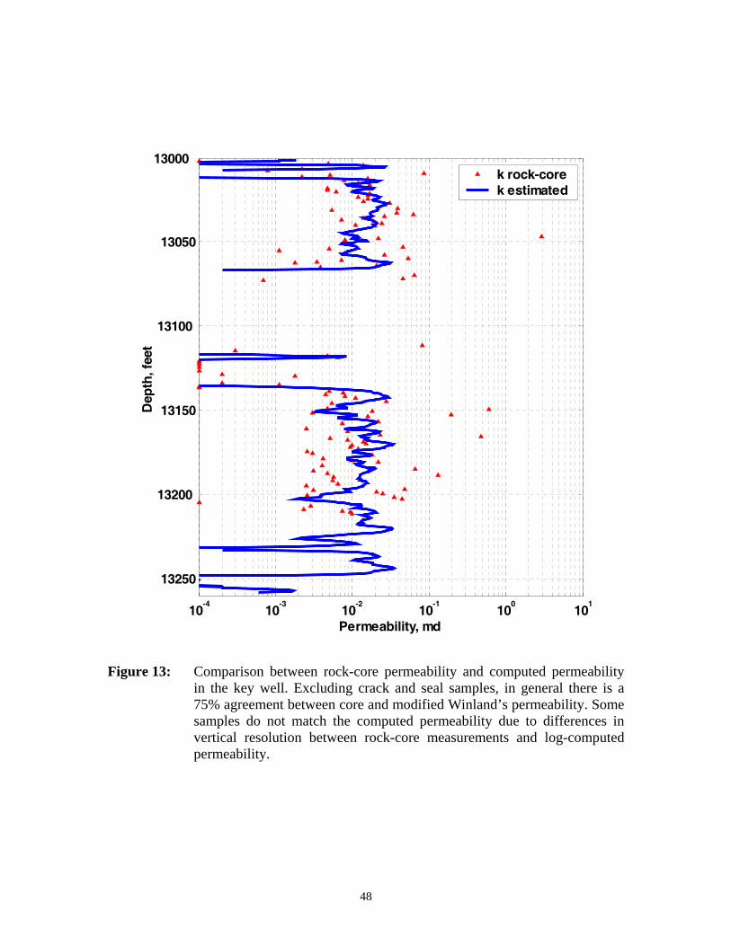
differences in vertical resolution. Figure 13 shows the average absolute permeability per
flow unit together with the rock-core Klinkenberg-corrected permeability at a confining
pressure of 2500 psi. A fair agreement is observed between rock-core and estimated
permeability. One important issue about the scatter of rock-core permeability compared
to the computed permeability is the differences of radial length of investigation and
vertical resolution of the measurements. Rock-core permeability only considers a small
plug of the rock while the computed permeability is estimated from induction logs whose
length of spatial support is considerable larger than that of a core plug.
§ Rock-core electrical measurements were available after the completion of the work reported in this paper. These measurements indicated that m varies between 1.91 and 2.26 (average = 2.15) and that n varies between 1.37 and 1.67 (average = 1.51). Electrical properties are extremely difficult to measure in tight-gas sands and are sometimes unreliable. However, the measured m values are very close to the values we used in this paper. On the other hand, n values are slightly different for rock 2A which is not as abundant as 1A. Sensitivity analysis proved that, due to the high connate water salt concentration (>200 kppm), slight variations of n do not substantially affect the estimation of water saturation.
18

We proceed to perform simulations of the process of mud-filtrate invasion in the
remaining two wells with the intent of estimating absolute permeability exclusively from
well logs. Petrophysical parameters other than porosity and permeability that are
necessary to simulate the process of mud-filtrate invasion are assumed to be the same as
those of the key cored well.
Estimation of Permeability Using the Physics of Mud-Filtrate Invasion
Two additional wells drilled in the same field and completed on the same
formation, here refereed to as Well 2 and Well 3, were available to perform petrophysical
assessments. These wells are located at a distance of 17 km and 1 km, respectively, from
the key well. Figure 14 shows the location of the two wells with respect to the key well.
High Definition Induction (HDIL**) and density-neutron logs are the only borehole
measurements available to estimate permeability in each well. Conventional
petrophysical interpretation is performed following the same methodology used in the
key well. Effective porosity is computed from the density log and the shale concentration
using the nonlinear model given by equation (3). Archie’s Law, equation (2), is used to
compute water saturation and the modified Winland equation (5) is used to obtain an
initial guess of absolute permeability. Based on the last three properties, together with the
corresponding Lorenz’s plots, flow units are defined for each well.
Simulation of Mud-Filtrate Invasion in Well 2. Following the same procedure
as in the key well, we performed simulations of the process of mud-filtrate invasion in
Well 2. Salinity of the drilling mud ranges from 5,000 to 7,500 ppm, that is to say, the
mud is fresher than the one used in Well 1. This mud creates an overbalance pressure of
** Mark of Baker Atlas
19

approximately 2,500 psi. All petrophysical properties estimated from logs (φ, Sw) and
extrapolated from rock-core data (kri, Pc) remain unchanged in the simulation. Absolute
permeability is the only varying parameter in each simulation of the process of mud-
filtrate invasion. For this well, 11 flow units were defined and then divided into 17
numerical layers to perform the simulation.
The estimation technique consists of performing the simulation by keeping
absolute permeability of each numerical layer as the only variable parameter.
Permeability is progressively adjusted until an acceptable match is found between the
estimated flushed-zone resistivity and the measured shallow resistivity (MOR1††). The
MOR1 has a radial length of investigation of approximately 10 inches. Therefore,
electrical resistivity values simulated at a radial distance of 10 inches within the
formation are used to assess the goodness of fit. Figure 15 shows radial profiles of water
saturation, salt concentration, and electrical resistivity taken in the middle of rock type
1A. After one day of invasion, the length of mud-filtrate invasion is 1.8 ft, and the
transition zone is approximately 0.8 ft-wide. A low resistivity annulus is also observed in
the radial profile of electrical resistivity. The latter can be attributed to the large contrast
of salt concentration between mud-filtrate and connate water.
Figure 16 graphically compares the measured and simulated values of Rxo. After
the first simulation, Rxo-sim agrees well with the field measurements. Thus, an adjustment
to permeability is not necessary. The latter exercise confirms the reliability of equation
(5) to estimate permeability from rock-core measurements. A comparison between the
averaged permeability per flow unit with the permeability computed with the modified
†† Mark of Baker Atlas
20

Winland model is shown in Figure 17. In this well, the initial guess is sufficient to
achieve a good agreement between the simulated electrical resistivity and the shallow
resistivity reading of the array induction instrument.
Simulation of Mud-Filtrate Invasion in Well 3. In a similar manner to Well 2,
we perform simulations of mud-filtrate invasion in Well 3. The salinity of the drilling
mud used in this well is between 3,000 and 4,500 ppm. Well 3 was drilled with the
freshest mud among the three wells under consideration. An overbalance pressure of
approximately 2,500 psi is sustained by the mud column. In this simulation, 32 numerical
layers are necessary to properly describe the process of mud-filtrate invasion across 17
flow units. In order to obtain the best estimate of absolute permeability for each layer,
multiple simulations are performed until securing a good agreement between the flushed-
zone resistivity and the shallow resistivity log.
From the radial invasion profiles shown in Figure 18, we observe a deeper
invasion of 2.3 ft and a wider transition zone (approximately 1.3 ft) compared to those of
Well 1 and Well 2. The fresh mud used to drill Well 3 is responsible for the occurrence of
a low resistivity annulus in the computed spatial distribution of electrical resistivity. A
big contrast between the salinity of mud-filtrate and connate water explains this
remarkable low resistivity region. Figure 19 shows that after the first simulation of the
process of mud-filtrate invasion, the agreement between the simulated and the measured
shallow resistivity is poor. Nevertheless, we keep adjusting the permeability for each
layer until achieving an acceptable match between the actual and simulated values of Rxo.
Figure 20 shows the agreement between the two resistivities after performing six
progressive adjustments to all the layer permeabilities. There are some intervals (13,020’-
21

13,050’) where the simulation of shallow resistivity does not agree well with the
measured Rxo. This discrepancy can be attributed to the high porosity observed in that
interval, ranging between 11 and 15%. Porosity does not exceed 11% in the remaining
segment of the formation. The high porosity is most likely due to anomalous density
measurements during logging operations. No explanation is available for this fact because
bulk density was measured at the same conditions as the rest of the available logs. The
best agreement between the measured and simulated resistivities is achieved across the
continuous homogeneous sandstones (Rocks 1A and 2A). Due to shoulder-bed effects, it
is not possible to secure a good agreement between simulated and measured resistivities
close to sand-shale boundaries. In addition, the large permeability contrast between
reservoir rocks (1A and 2A), and non-reservoir rocks (3A and impermeable shale layers),
makes it very difficult to reach a good agreement between the simulated and the
measured values of Rxo.
Based on the match of simulated and measured shallow resistivity, we obtain the
final estimate of permeability shown in Figure 21. In general, the new estimation is 50 to
80% higher than the initial guess. For a few segments (2 layers) the estimated value of
permeability is 5 to 10% below the initial guess. Sensitivity analysis to assess the effect
of flow rate on the estimation of permeability was performed by changing the
permeability of mudcake. Permeability of mudcake was increased from 25% to 100%.
Shallow resistivity exhibits increments between 2% to 8% for these flow rates. The latter
implies that the estimated values of permeability increase approximately by 10% for
increments of 100% in the flow rate of mud-filtrate invasion. Figure 22 shows the error in
22

the estimation of absolute permeability due to a change of ±50% in the initial
permeability of mudcake.
Even though this analysis is based on a cored key well, the study can be
performed using standard suites of well logs (gamma ray, resistivity, and neutron-
density) along with NMR logs. In so doing, relative permeability curves could be
calculated using the Brooks-Corey equations described in Appendix A.
Discussion
The methodology described in this paper to estimate permeability requires that
relative permeability, capillary pressure, and Archie’s parameters be known a priori. It is
also required that mud properties, time of invasion, formation pressure, and overbalance
pressure be available from ancillary mud logs and static tests of mud-filtrate invasion
performed uphole with a paper filter. The model used to reproduce the process of mud-
filtrate invasion assumes an immiscible fluid flow process between mud-filtrate, connate
water, and hydrocarbon. In addition, the invasion process takes into account the
progressive thickening of mudcake, the ensuing reduction of mudcake permeability, and
the coupling of mudcake buildup with rock formations. A crucial component of the
simulations is the dynamic mixing of salt between mud filtrate and connate water. Salt
mixing controls the radial variations of formation resistivity away from the borehole wall
and hence has a strong influence on borehole resistivity measurements.
Further, the estimation procedure assumes that capillary pressure and relative
permeability data, along with fluid properties, are available from laboratory
measurements of rock-core samples retrieved from a key cored well. These parameters
can be specific to a given flow unit but are assumed spatially constant within the
23

hydrocarbon field under consideration within the same geological unit. The availability of
petrophysical and rock fluid properties in the key well, including permeability, provides a
way to “calibrate” the invasion model and hence to refine the estimates of time of
invasion and Archie’s parameters associated with a specific flow unit. The estimated
Archie’s parameters and the measured relative permeability and capillary pressure curves
are used in all of the remaining wells to perform local simulations of the process of mud-
filtrate invasion. Specific parameters necessary for the simulation of mud-filtrate invasion
in each well include porosity, mud properties (including salt concentration), overbalance
pressure, and time of invasion. Porosity is estimated from bulk density, neutron, and
resistivity logs, while time of invasion is inferred by enforcing a global agreement
between simulated shallow, medium, and deep formation resistivity values and the
corresponding measured resistivity logs.
Clearly, errors and uncertainties in all of the assumed parameters will translate
into errors in the estimated permeability. The only possible manner to quantify the
influence of errors in the assumed petrophysical parameters on the calculated
permeability is to perform a systematic sensitivity analysis. Despite these technical
difficulties, the attractive components of the estimation of permeability based on the
physics of mud filtrate invasion are: (a) the petrophysical model itself is consistent with
the physics of multi-phase fluid flow displacement in the borehole region, (b) the
estimated permeability honors all of the available measurements, and (c) the estimated
permeability is consistent with the radial length of investigation and vertical resolution of
well logs and, therefore, provides an “upscaled” version of permeability compared to that
of rock-core samples.
24

To date, permeability remains one of the most difficult petrophysical variables to
measure and/or estimate from indirect measurements. A traditional means to estimate
permeability from well logs includes the use of porosity-permeability regressions
performed on rock-core measurements and extrapolated to uncored wells via well logs. It
is also possible to use elemental analysis based on complete suites of logs and
petrophysical models that require extensive core calibration. Yet another recently popular
procedure is the multi-linear regression of well logs with core calibration. A variation of
this method includes the use of artificial neural networks. While the above methods are
relatively simple to develop and implement, they are seldom subject to cross-validation
and/or checks of petrophysical consistency, nor are they required to honor the scales of
spatial resolution and length of investigation of the different measurements involved in
the estimation.
The estimation procedure described in this paper offers a general model that,
despite its difficulties and associated parameter uncertainty, could be applied to a wide
variety of rock formations, including carbonates, unconsolidated sands, and naturally
fractured rocks. It could also be used in combination with direct measurements of
permeability performed with formation testers to further calibrate Archie’s parameters,
fluid viscosity, capillary pressure, and relative permeability. Finally, the estimation
method based on the physics of mud-filtrate invasion easily lends itself to the use of time-
lapse data, such as a combination of logging-while-drilling and openhole logs, to improve
the accuracy and reliability of the calculated values of permeability. An automatic
inversion procedure is in order to perform the adjustments of permeability with an
efficient minimization method such as those used in the field of geophysical inverse
25

theory. Further conceptual and algorithmic developments are needed to apply the
estimation technique in wells drilled with an oil-based mud.
Conclusions
We have developed and tested a new methodology to estimate absolute
permeability in wells for which the only available measurements is a basic suite of well
logs. The technique was tested on a set of three wells penetrating the tight-gas sands in
the Bossier formation of East Texas. One of the three wells was cored along the sand
deposits of interest and the corresponding rock-core measurements were used to calibrate
the petrophysical invasion model. Simulations were performed of the process of mud-
filtrate invasion in the uncored wells in order to reproduce the measured resistivity logs.
In so doing, the permeability of flow units was progressively adjusted until the simulated
formation resistivity in the invaded zone agreed with the corresponding shallow
resistivity readings.
In general, traditional permeability estimation methods, such as Winland, Tixier,
Timur, etc, are not reliable in tight-gas rocks. The estimation technique developed in this
paper allowed us to cross-validate and calibrate the invasion model against existing rock-
core measurements in the key well. Such a step provided us with improved estimates of
time of invasion and of Archie’s electrical resistivity-water saturation parameters. The
estimated permeability values in one of the uncored wells were consistent with the
porosity-permeability correlation established in the cored key well. However, the
estimated permeability values in the second uncored well were 50-80% higher than
predicted with the same porosity-permeability correlation.
26

Even though the test examples considered in this paper are non-trivial from the
petrophysical point of view (tight-gas sands) and the results are encouraging, additional
testing and cross-validation exercises with field data are necessary to render the
estimation process more efficient and reliable. For instance, it is necessary to thoroughly
assess the influence of imprecise mud parameters, mudcake growth models, errors in the
time of invasion, and biased rock-fluid properties on the estimated values of permeability.
Also, we remark that additional studies are necessary to assess the relative benefits of the
proposed technique for the petrophysical assessment of carbonate formations.
Acknowledgements
We are obliged to Anadarko Petroleum Corporation for permission to publish
these results. A note of special gratitude goes to Dr. E.C. Thomas and three anonymous
reviewers whose constructive and illuminating feedback helped to improve the original
manuscript. Funding for the work reported in this paper was provided by UT Austin’s
Research Consortium on Formation Evaluation, jointly sponsored by Anadarko
Petroleum Corporation, Baker Atlas, ConocoPhillips, ExxonMobil, Halliburton, Mexican
Institute for Petroleum, Schlumberger, Shell International E&P, and TOTAL.
Nomenclature
a : tortuosity factor, [ ]
A : Cross-sectional area, [ft2]
enw : empirical exponents for krnw equation, [ ]
ep : pore-size distribution exponent, [ ]
ew : empirical exponents for krw equation, [ ]
27

hmc : mudcake thickness, [ft]
k : absolute permeability, [md ]
kmc : mudcake permeability, [md]
krnw : non-wetting-phase relative permeability, [ ]
krnw0 : krnw end point, [ ]
krw : wetting-phase relative permeability, [ ]
krw0 : krw end point, [ ]
m : cementation exponent, [ ]
n : saturation exponent, [ ]
Pc : capillary pressure, [psi]
Pco : coefficient for capillary pressure, [psi.darcy1/2]
ΔP : pressure drop across the mudcake, [psi]
Qf : flow rate of mud-filtrate across the borehole wall, [ft3/day]
r : pore-throat aperture size, [μm]
Rt : true formation resistivity, [Ohm.m]
Rw : connate water resistivity, [Ohm.m]
Rxo : measured shallow (flushed-zone) resistivity, [Ohm.m]
Rxo-sim : simulated shallow (flushed-zone) resistivity, [Ohm.m]
S : surface area, [μm2]
SN : normalized wetting-phase saturation, [fraction]
Sw : water saturation, [fraction]
T : temperature, [oF]
T2 : rate of decay of transverse magnetization, [ms]
Vsh : volume of shale concentration, [fraction]
[NaCl] : equivalent NaCl concentration (salinity), [ppm]
μf : mud-filtrate viscosity, [cp]
φ : effective porosity, [fraction]
θ : contact angle, [degrees]
ρ1, ρ2 : fluid density, [g/cm3]
ρb : bulk density, [g/cm3]
28

ρma : matrix density, [g/cm3]
ρsh : shale density, [g/cm3]
σ : surface tension, [dynes/cm]
References
1. Altunbay, M., Martain, R., and Robinson, M., “Capillary Pressure Data From NMR
Logs and Its Implications on Field Economics,” paper SPE 71703 presented at the
SPE Annual Technical Conference and Exhibition, New Orleans, Louisiana,
September 30–October 3, 2001.
2. Balan, B., Mohagheh, S., and Armeri, S., “State-of-The-Art in Permeability
Determination From Well Log Data: Part 1- A Comparative Study, Model
Development,” paper SPE 30978 presented at the SPE Eastern Regional Conference
and Exhibition, Morgantown, West Virginia, September 17-21, 1995.
3. Bigelow, Ed., “Introduction to Wireline Log Analysis,” Western Atlas International,
Inc., Houston, Texas, 1992.
4. Corey, A.T., “Mechanics of Immiscible Fluids in Porous Media,” Water Resource
Publications, Highland Ranch, Colorado, 1994.
5. Delshad, M, Pope, G.A., and Sepehrnoori, K., “A Compositional Simulator for
Modelling Surfactant Enhanced Aquifer Remediation,” Journal of Contaminant
Hydrogeology, v. 23, 1996, p. 303-327.
6. George, B.K., Torres-Verdin, C., Delshad, M., Sigal, R., Zouioueche, F., and
Anderson, B., “Assesment of In-Situ Hydrocarbon Saturation in the Presence of
Deep Invasion and Highly Saline Connate Water,” Petrophysics, v. 45, No 2,
March-April 2004, p. 141-156.
29

7. Gunter, G.W., Finneran, J.M., Hartmann, D.J. and Miller, J.D., “Early
Determination of Reservoir Flow Units Using an Integrated Petrophysical Method,”
paper SPE 38679 presented at the SPE Annual Technical Conference and
Exhibition, San Antonio, Texas, October 5-8, 1997.
8. Klein, G.D. and Chaivre, K.R., “Sequence and Seismic Stratigraphy of the Bossier
Formation (Tithonian), Western East Texas Basin,” Gulf Coast Association of
Geological Societies Transactions, v. 52, 2002, p. 551-561.
9. Lake, L. W., “Enhanced Oil Recovery,” Prentice Hall, Upper Saddle River, New
Jersey, 1989.
10. Newsham, K.E., Rushing, J.A., “Laboratory and Field Observations of an Apparent
Sub Capillary-Equilibrium Water Saturation Distribution in a Tight Gas Sand
Reservoir,” paper SPE 75710 presented at the SPE Gas Technology Symposium,
Calgary, Alberta, Canada, April 30-May 2, 2002.
11. Pittman, E.D., “Relationship of Porosity and permeability to Various Parameters
Derived from Mercury Injection Capilary Pressure Curve for Sandstones,” AAPG
Bulletin, v. 76, No 2, 1992, p. 191-198.
12. Proett, M.A., Chin, W.C., Manohar, M., Sigal, R. and Wu, J., “Multiple Factors that
Influence Wireline Formation Tester Pressure Measurements and Fluid Contacts
Estimates,” paper SPE 71566 presented at the SPE Annual Technical Conference
and Exhibition, New Orleans, Louisiana, September 30-October 3, 2001.
13. Showalter, T.T., “Mechanics of Secondary Hydrocarbon Migration and
Entrapment,” AAPG Bulletin, v. 63, No 5, May 1979, p. 723-760.
30
14. Thomas, E.C. and Stieber S.J., “The distribution of shale in sandstones and its
effects upon porosity,” paper T presented at the SPWLA Sixteenth Annual Logging
Symposium, New Orleans, Louisiana, June 4-7, 1975.
15. Williams, R.A., Robinson, M.C., Fernandez, E.G., and Mitchum, R.M., “Cotton
Valley/Bossier of East Texas: Sequence Stratigraphy Recreates the Depositional
History,” Gulf Coast Association of Geological Societies Transactions, v. 51, 2001,
p. 379-388.
16. Wu, J, Torres-Verdin, C., Sepehrnoori, K., and Delshad, M., “Numerical Simulation
of Mud Filtrate Invasion in Deviated Wells,” SPE Reservoir Evaluation &
Engineering, v. 7, No 2, April 2004, p. 143-154.
Appendix
A. - Capillary Pressure and Relative Permeability Models
A method to compute capillary pressure of a two-phase fluid mixture was
introduced by Brooks and Corey (1966). They proposed that the first imbibition cycle of
the capillary pressure curve could be written as
( ) ,1 peN
occ S
kPP −=
φ (A.1)
31
where Pc is capillary pressure, Pco is the coefficient for capillary pressure, ep is the pore-
size distribution exponent, φ is porosity, k is permeability, and SN is the normalized
wetting phase saturation, given by
,1 nwrwr
wrwN SS
SSS
−−−
= (A.2)
where Swr and Snwr are the residual wetting and non-wetting phase saturations,
respectively.
Multiphase imbibition and drainage relative permeability curves in the saturated
zone can also be calculated using Brooks-Corey’s equations, namely,
,0 weNrwrw Skk = (A.3)
and
( ) ,10 nweNrnwrnw Skk −= (A.4)
where krw and krnw are wetting and non-wetting relative permeabilities, and are
relative permeability end points, and e
0rwk 0
rnwk
w and enw are empirical exponents for each fluid
phase. Figure A.1 shows relative permeability curves calculated with equations (A.3) and
(A.4), along with the only available laboratory gas relative permeability curve available
for the study reported in this paper. The laboratory data do not reach irreducible water
saturation conditions (Sw = 0-5%) due to a low gas-injection rate that induces gas
condensation in the porous rock-core sample.
32
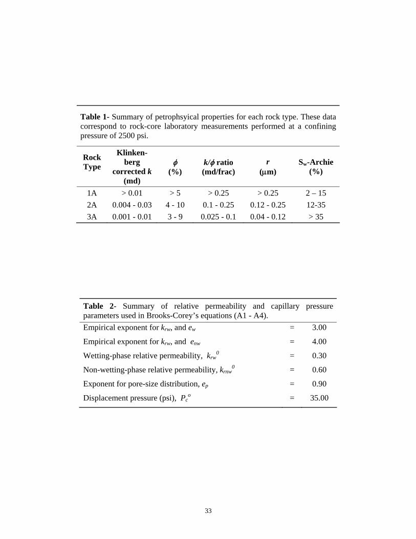
Table 1- Summary of petrophsyical properties for each rock type. These data correspond to rock-core laboratory measurements performed at a confining pressure of 2500 psi.
Rock Type
Klinken-berg
corrected k (md)
φ (%)
k/φ ratio (md/frac)
r (μm)
Sw-Archie (%)
1A > 0.01 > 5 > 0.25 > 0.25 2 – 15 2A 0.004 - 0.03 4 - 10 0.1 - 0.25 0.12 - 0.25 12-35 3A 0.001 - 0.01 3 - 9 0.025 - 0.1 0.04 - 0.12 > 35
Table 2- Summary of relative permeability and capillary pressure parameters used in Brooks-Corey’s equations (A1 - A4). Empirical exponent for krw, and ew = 3.00
Empirical exponent for krw, and enw = 4.00
Wetting-phase relative permeability, krw0 = 0.30
Non-wetting-phase relative permeability, krnw0 = 0.60
Exponent for pore-size distribution, ep = 0.90
Displacement pressure (psi), Pco = 35.00
33

Table 3- Summary of measured mud properties for the key well.
Depth (ft)
Mud Weight (ppg)
Viscosity (s/qt) pH
Filtrate Loss
(cm3/30min)
NaCl (ppm)
Solids (%)
12982 14.0 123 7.4 1.1 20000 24.7
13023 14.0 90 7.5 1.2 25000 22.3
13054 14.2 105 7.6 1.1 30000 22.0
13066 14.3 95 7.6 1.2 30000 22.0
13090 13.8 82 7.7 1.2 34000 21.7
13109 13.4 75 7.3 1.3 35000 19.6
13150 13.3 92 7.5 1.2 36000 19.5
13194 13.9 90 7.4 1.1 33000 21.8
13214 13.8 96 7.5 1.1 33000 22.8
13285 13.9 96 7.2 1.2 33000 22.8
34

0.00
0.05
0.10
0.15
0.20
0.001 0.01 0.1 1r, μm
Inc.
Hg
Sat.,
frac
tion
pore
spa
ce3-1 HS13-19 HS14-2 HS14-11 HS12-41 HS14-15 HS16-21 HS16-25 HS16-6 HS16-32 HS1*6-34 HS17-16 HS2
Rock Type 1A
Rock Type 2A
Rock Type 3A
Figure 1: Incremental mercury intrusion plot obtained from capillary pressure curves. The maximum of each curve indicates the dominant pore throat aperture and discriminates the rock type (RT). For instance, RT 1A (shown in red) has r > 0.25 μm, RT 2A (shown in blue) ranges between 0.12 - 0.25 μm, and RT 3A (shown in yellow) r < 0.1 μm. The legend identifies specific rock-core samples.
35
1.E-04
1.E-03
1.E-02
1.E-01
1.E+00
0 3 6 9 12Porosity, %
Perm
eabi
lity,
mD
k, Klinkenberg CorrectedPc Samples
10
5.0
1.0
k/φ
0.25
0.01
0.05
0.5
2.5
0.025
md/frac
1A
2A
3A
Cracked Samples
0.1
1A
2A
3A
Rock Type
Seals
Figure 2: Porosity-permeability cross-plot showing parametric curves of constant
k/φ ratios. Parametric curves clearly define three different rock types (large rectangles). Triangular symbols represent samples with capillary pressure measurements. The oval shown in the top of the figure identifies cracked samples which were not used in the analysis, and the oval at the bottom of the figure identifies seal and baffle zones.
36

1.E+02
1.E+03
1.E+04
0.00.20.40.60.81.0Mercury Saturation, fraction pore space
Inje
ctio
n Pr
essu
re, p
si
3-1 HS13-19 HS14-2 HS14-11 HS12-41 HS14-15 HS16-21 HS16-25 HS16-6 HS16-32 HS1*6-34 HS17-16 HS2
RT 2A
RT 3A
RT 1A
Figure 3: Curves of selected rock-core measurements of mercury injection capillary pressure. Note that the capillary pressure curves confirm the presence of three distinct rock types.
37

10-1
100
101
102
103
104
0
0.1
0.2
0.3
0.4
0.5
0.6
0.7
0.8
Incr
emen
tal
Po
rosi
ty,
frac
cio
n
T2, ms
Sample 3-19, RT 1ASample 4-2, RT 1ASample 6-21, RT 2ASample 6-32, RT 3A
Figure 4: NMR Transverse relaxation, T2, curves for different rock types. Each rock type is associated with a specific range of dominant T2.
38

0 0.2 0.4 0.6 0.8 10
0.2
0.4
0.6
0.8
1
Cu
m. F
low
Cap
acit
y, f
ract
ion
0 0.2 0.4 0.6 0.8 1
13050
13100
13150
13200
13250
0 0.2 0.4 0.6 0.8 10
0.2
0.4
0.6
0.8
1
Cum. Storage Capacity, fraction
Continuous SLMPInterpreted SLMP
MLP
(a)
(b)
Depth, ft
Figure 5: Flow unit identification in the key well based on storage and flow
capacity. (a) Interpreted Continuous Stratigraphic Modified Lorenz Plot: slope changes define flow units, (b) Modified Lorenz Plots: sorting by quality, the steeper the slope the higher the storage and flow capacity of the flow unit.
39

0 10 20 30 40 50 60 70 80 90 1000
1
2
3
4
5
6
7
8
9
10
Volume of shale concentration, %
Po
rosi
ty, %
Rock-core measurements
Dispersed Laminated
Structural
Figure 6: Thomas-Stieber cross-plot used to diagnose the type of shale/clay distribution across the sand units of interest. Rock-core XRD measurements are used as indicators of shale concentration. The cross-plot indicates that dispersed shale is the dominant type of shale/clay distribution in the sand units.
40

0 0.2 0.4 0.6 0.8 1-1.4
-1.3
-1.2
-1.1
-1
-0.9
-0.8
-0.7
-0.6
-0.5
-0.4
log
(r)
Water Saturation, fraction
log(r)linear(log(r))
log(r) = - 0.9323Sw - 0.389
R2 = 0.9372
Figure 7: The logarithm of pore throat aperture (r) as a function of water saturation (Sw) estimated from capillary pressure curves. The constants in Equation (6) were derived using a linear least-squares regression that relates r with log-computed Sw.
41
T2 (ms)φh
kh
k/φ
YORK
BONNER
T2 (ms)φh
kh
k/φ
YORK
BONNER
42
Figure 8: Petrophysical Assessment. Track 1: lithology logs and core grain density. Track 2: array induction resistivity logs. Track 3: modified Winland’s permeability (shown with a continuous line), core permeability (shown with diamonds), and NMR permeability (shown with squares). Track 4: neutron-density data highlighting gas zones (shown with shading). Track 5: calculated effective porosity (shown with a continuous line) and core porosity (shown with diamonds). Track 6: Archie’s water saturation and core Dean-Stark water saturation. Tracks 7 and 8: Stratigraphic Flow Profile and identified flow units. Track 9: NMR T2 distribution displays only one maximum; this indicates negligible irreducible water saturation. Track 10: volumetric analysis showing clean sands in the Bonner member and more heterogeneous sands in the York member. X-Ray Diffraction mineralogy measurements are consistent with the computed shale volume.
.
43

Flow Units Simulation Grid
Wellbore
ρ
z
Figure 9: Geometrical description of the borehole and formation model. The figure
shows the flow units and the numerical finite-difference grid used in the simulations of mud-filtrate invasion. Each flow unit and/or numerical layer is associated with specific petrophysical properties. The simulation grid used in Well 1 consists of 61x10 nodes in the radial (ρ) and vertical (z) direction for the Bonner member, and of 61x20 nodes for the York member.
44

0 0.5 1 1.5 2 2.5 30
0.5
1
Wat
er S
atu
rati
on
, fr
acWell 1, Rock 1A, INVADE Results
0 0.5 1 1.5 2 2.5 30
50
100
150
200
Sal
init
y, k
pp
m
0 0.5 1 1.5 2 2.5 310
0
102
Radial Distance, ft
0.25 day1 day1.5 days2 days
Res
isti
vity
, O
hm
-m
Figure 10: Results from the simulation of mud-filtrate invasion in the key well for
Rock Type 1A. The plots describe the dynamic evolution in the radial direction of water saturation, salt concentration, and electrical resistivity with time of invasion. From top to bottom: water saturation, salt concentration, and electrical resistivity. Radial distances are measured from the borehole wall.
45

0 0.5 1 1.5 2 2.5 30
0.5
1
Wat
er S
atu
rati
on
, fr
ac
Well 1, Rock 2A, INVADE Results
0 0.5 1 1.5 2 2.5 30
50
100
150
200
Sal
init
y, k
pp
m
0 0.5 1 1.5 2 2.5 310
0
102
Radial Distance, ft
0.25 day1 day1.5 days2 days
Res
isti
vity
, O
hm
-m
Figure 11: Results from the simulation of mud-filtrate invasion in the key well for the Rock Type 2A. The plots describe the dynamic evolution in the radial direction of water saturation, salt concentration, and electrical resistivity with time of invasion. From top to bottom: water saturation, salt concentration, and electrical resistivity. Radial distances are measured from the borehole wall.
46

100
101
102
103
13000
13050
13100
13150
13200
13250
Dep
th, f
eet
Resistivity, Ohm.m
HO24Rxo-Sim
Rock Type
Figure 12: Comparison of measured (HO24) and simulated shallow resistivity (Rxo_Sim) logs in Well 1, together with the description of flow units (1A=1, 2A=2, 3A=3, and shale=4). Archie’s m and n exponents are varied until Rxo_Sim agrees with HO24. The best agreement is obtained in the most homogeneous sand (Bonner group).
47
10-4
10-3
10-2
10-1
100
101
13000
13050
13100
13150
13200
13250
Dep
th, f
eet
Permeability, md
k rock-corek estimated
Figure 13: Comparison between rock-core permeability and computed permeability in the key well. Excluding crack and seal samples, in general there is a 75% agreement between core and modified Winland’s permeability. Some samples do not match the computed permeability due to differences in vertical resolution between rock-core measurements and log-computed permeability.
48

Well Locations
11490000
11492000
11494000
11496000
11498000
11500000
11502000
11504000
2540000 2542000 2544000 2546000 2548000 2550000 2552000 2554000 2556000
N
2 km
Well 1Well 3
Well 2
Figure 14: Relative locations of the wells considered in this paper. Well 1 is the key cored well and Well Nos. 2 and 3 are development wells that include a basic suite of logs but lack rock-core measurements.
49

0 0.5 1 1.5 2 2.5 30
0.5
1W
ater
Sat
ura
tio
n,
frac
Well 2, Rock 1A, INVADE Results after 1 day
0 0.5 1 1.5 2 2.5 30
50
100
150
200
Sal
init
y, k
pp
m
0 0.5 1 1.5 2 2.5 310
0
102
Radial Distance, ft
Res
isti
vity
, O
hm
-m
Figure 15: Results from the simulation of mud-filtrate invasion in Well 2 after 1 day of invasion for Rock Type 1A. The time of invasion is 1 day. From top to bottom: radial profiles of water saturation, salt concentration, and electrical resistivity measured from the borehole wall. The radial length of investigation of MOR1 measurements is between 10 to 14 inches (0.833 to 1.167 ft). A low resistivity annulus due to low mud-filtrate salinity is observed in the transition zone.
50

100
101
102
103
12500
12550
12600
12650
Dep
th, f
eet
Resistivity, Ohm.m
MOR1Rxo-Sim
Rock Type
Figure 16: Comparison of measured (MOR1) and simulated shallow resistivity
(Rxo_Sim) curves in Well 2. The simulated curve agrees well with the measured log.
51

10-3
10-2
10-1
12500
12550
12600
12650
Dep
th, f
eet
Permeability, md
k calculated (initial guess)k estimated
Figure 17: Comparison of the modified Winland’s permeability (initial guess) and the permeability estimated by matching Rxo via the numerical simulation of the process of mud-filtrate invasion in Well 2.
52

0 0.5 1 1.5 2 2.5 30
0.5
1W
ater
Sat
ura
tio
n,
frac
Well 3, Rock 1A, INVADE Results after 1 day
0 0.5 1 1.5 2 2.5 30
50
100
150
200
Sal
init
y, k
pp
m
0 0.5 1 1.5 2 2.5 310
0
102
Radial Distance, ft
Res
isti
vity
, O
hm
-m
Figure 18: Results from the simulation of mud-filtrate invasion in Well 3 after 1 day of invasion for rock type 1A. From top to bottom: radial profiles of water saturation, salt concentration, and electrical resistivity measured from the borehole wall. Due to the high salinity contrast between mud-filtrate and connate water, the resistivity annulus is more pronounced in this well than in Wells 1 and 2.
53

100
101
102
103
104
12950
13000
13050
13100
13150
Dep
th, f
eet
Resistivity, Ohm.m
MOR1Rxo-Sim
Rock Type
Figure 19: Comparison of measured and simulated shallow resistivity readings using the initial guess of permeability in Well 3. The measured and simulated resistivities do not agree with each other.
54

100
101
102
103
12950
13000
13050
13100
13150
Dep
th, f
eet
Resistivity, Ohm.m
MOR1Rxo-Sim
Rock Type
Figure 20: Comparison of measured and simulated shallow resistivity readings in
Well 3 after six progressive adjustments to the permeabilities of flow units. A good agreement between measured and simulated resistivities is obtained in the homogeneous sand layers.
55

10-3
10-2
10-1
100
12950
13000
13050
13100
13150
Dep
th, f
eet
Permeability, md
k calculated (initial guess)k estimated
Figure 21: Comparison of the modified Winland’s permeability (initial guess) and the permeability estimated by matching Rxo obtained via the numerical simulation of mud-filtrate invasion in Well 3. Six progressive adjustments to the permeability of flow units were necessary to calculate the final permeability curve shown above. In general, the values of permeability estimated by matching the shallow resistivity readings, Rxo, are higher than those of the initial guess.
56

10-3
10-2
10-1
12970
12980
12990
13000
13010
13020
Dep
th, f
eet
Permeability, md
k calculated (initial guess)k estimatedk error
Figure 22: Permeability estimate for an interval in Well 3 displaying the error after a perturbation in the permeability of mudcake. The error in the estimation of permeability is approximately 5% for a change of ±50% in the permeability of mudcake.
57

0 0.2 0.4 0.6 0.8 10
0.2
0.4
0.6
0.8
1
Rel
ativ
e P
erm
eab
ility
, fra
ctio
n
Wetting Phase Saturation, fraction
krg Measuredkrnwkrw
Figure A.1: Water-gas Brooks-Corey type relative permeability curves, along with the measured gas relative permeability curve. The experimental measurements do not reach irreducible water saturation conditions (0-5%). Such behavior could be attributed to limitations of the laboratory equipment used to inject the gas at a rate sufficiently high to avoid gas condensation. Therefore, the rock sample cannot be totally dried and remains partially water-saturated.
58
ABOUT THE AUTHORS
Jesus M. Salazar is a Research Assistant and a PhD student in the Department of
Petroleum and Geosystems Engineering at The University of Texas at Austin. He
received a BS in Physics (with honors) from Universidad Central de Venezuela in 1998
and a MSE in Petroleum Engineering from The University of Texas at Austin in 2004.
From 1997 to 2002 he worked for PDVSA (Maracaibo, Venezuela) as a petrophysicist
and well log analyst. He was bestowed a student grant, 2002-2003, and two scholarships,
2003-2004 and 2005-2006 by the SPWLA. His research interests include petrophysics,
log analysis, inverse problems, and numerical reservoir simulation.
Carlos Torres-Verdín received a PhD in Engineering Geoscience from the University of
California, Berkeley, in 1991. During 1991–1997 he held the position of Research
Scientist with Schlumberger-Doll Research. From 1997–1999, he was Reservoir
Specialist and Technology Champion with YPF (Buenos Aires, Argentina). Since 1999,
he has been with the Department of Petroleum and Geosystems Engineering of The
University of Texas at Austin, where he currently holds the position of Associate
Professor. He conducts research on borehole geophysics, formation evaluation, and
integrated reservoir characterization. Torres-Verdín has served as Guest Editor for Radio
Science, and is currently a member of the Editorial Board of the Journal of
Electromagnetic Waves and Applications, and an associate editor for Petrophysics
(SPWLA) and the SPE Journal.
59
Richard Sigal is currently a Research Professor at the University of Oklahoma with a
joint appointment in the Petroleum Engineering and Geoscience Departments. He is also
the Director of the Mobile Core Analysis Laboratory at Oklahoma University.
Previously, Richard worked for Anadarko as part of the engineering technology group.
Before joining Anadarko he spent 21 years with Amoco mostly in their Tulsa Technology
Center. After retiring from Amoco, he worked for two years for Halliburton in Houston.
During the last 15 years, much of Richard’s time has been spent on understanding
permeability and the technologies used to characterize and estimate it. He worked in
Petrophysics and core measurements at Amoco and supervised the development of
Petrophysical applications at Halliburton. Among his areas of special expertise are NMR
and mercury capillary pressure measurements. Richard was trained in mathematics and
physics. His PhD thesis from Yeshiva University was in general relativity.
60