Embed Size (px)
Citation preview

328
Maurer, B. W. et al. (2015). Geotechnique 65, No. 5, 328–336 [http://dx.doi.org/10.1680/geot.SIP.15.P.007]
Assessment of CPT-based methods for liquefaction evaluation in aliquefaction potential index framework
B. W. MAURER�, R . A. GREEN�, M. CUBRINOVSKI† and B. A. BRADLEY†
In practice, several competing liquefaction evaluation procedures (LEPs) are used to compute factorsof safety against soil liquefaction, often for use within a liquefaction potential index (LPI) frameworkto assess liquefaction hazard. At present, the influence of the selected LEP on the accuracy of LPIhazard assessment is unknown, and the need for LEP-specific calibrations of the LPI hazard scale hasnever been thoroughly investigated. Therefore, the aim of this study is to assess the efficacy of threeCPT-based LEPs from the literature, operating within the LPI framework, for predicting the severityof liquefaction manifestation. Utilising more than 7000 liquefaction case studies from the 2010–2011Canterbury (NZ) earthquake sequence, this study found that: (a) the relationship between liquefactionmanifestation severity and computed LPI values is LEP-specific; (b) using a calibrated, LEP-specifichazard scale, the performance of the LPI models is essentially equivalent; and (c) the existing LPIframework has inherent limitations, resulting in inconsistent severity predictions against field observa-tions for certain soil profiles, regardless of which LEP is used. It is unlikely that revisions of theLEPs will completely resolve these erroneous assessments. Rather, a revised index which moreadequately accounts for the mechanics of liquefaction manifestation is needed.
KEYWORDS: earthquakes; liquefaction; sands; seismicity
INTRODUCTIONThe objective of this study is to assess the efficacy of threecommon cone penetration test (CPT)-based liquefaction eva-luation procedures (LEPs), operating within a liquefactionpotential index (LPI) framework, for predicting the severityof surficial liquefaction manifestation, which is commonlyused as a proxy for liquefaction damage potential. Utilisingdata from the 2010–2011 Canterbury earthquakes, this studyinvestigates the influence of the selected LEP on the accu-racy of hazard assessments, and assesses the need for LEP-specific calibrations of the LPI hazard scale. Towards thisend, the deterministic LEPs of Robertson & Wride (1998)(R&W98), Moss et al. (2006) (MEA06), and Idriss &Boulanger (2008) (I&B08) are evaluated.
While the ‘simplified’ LEP (Seed & Idriss, 1971; Whit-man, 1971) is central to most liquefaction hazard assess-ments, the output from an LEP is not a direct quantificationof liquefaction damage potential, but rather is the factor ofsafety against liquefaction triggering (FSliq) in a soil stratumat depth. Iwasaki et al. (1978) proposed the LPI to linkliquefaction triggering at depth to damage potential, whereLPI is computed as
LPI ¼ð20 m
0
Fw(z)dz (1)
where F ¼ 1 � FSliq for FSliq < 1 and F ¼ 0 for FSliq . 1;w(z) is a depth weighting function given by w(z) ¼ 10 � 0.5z;and z is depth in metres below the ground surface. Thus, it is
assumed that the severity of liquefaction manifestation isproportional to the thickness of a liquefied layer, the proxi-mity of the layer to the ground surface, and the amount bywhich FSliq is less than 1.0. Given this definition, LPI canrange from 0 to a maximum of 100 (i.e. where FSliq is zeroover the entire 20 m depth). Analysing SPT data from 55sites in Japan, Iwasaki et al. (1978) proposed that severeliquefaction should be expected for sites where LPI . 15 butnot where LPI , 5. This criterion for liquefaction manifesta-tion, defined by two threshold values of LPI, is subsequentlyreferred to as the Iwasaki criterion. However, in using theLPI framework to assess liquefaction hazard in current prac-tice, it is not always appreciated that the Iwasaki criterion isinherently linked to the LEP that was in common use inJapan in 1978, which differs significantly from those com-monly used today. Also, it has been shown that the variousLEPs used in today’s practice can result in different FSliq
values for the same soil profile and earthquake scenario (e.g.Green et al., 2014), and thus different LPI values. Thesedifferences have led to confusion as to which LEP is the mostaccurate, and whether the Iwasaki criterion is equally effec-tive for all LEPs.
The 2010–2011 Canterbury earthquake sequence (CES)resulted in a liquefaction dataset of unprecedented size andquality, presenting a unique opportunity to assess the effi-cacy of liquefaction analytics (e.g. Cubrinovski & Green,2010; Cubrinovski et al., 2011; Bradley & Cubrinovski,2011). Towards this end, Maurer et al. (2014) evaluated LPIduring the CES at approximately 1200 sites using theR&W98 CPT-based LEP. Although the Iwasaki criterion wasfound to be effective in a general sense, LPI hazard assess-ments were erroneous for a portion of the study area. Inpractice, several competing LEPs are used to assess liquefac-tion hazard in an LPI framework (e.g. Sonmez, 2003; Toprak& Holzer, 2003; Baise et al., 2006; Holzer et al., 2006a,2006b; Lenz & Baise, 2007; Cramer et al., 2008; Hayati &Andrus, 2008; Holzer, 2008; Chung & Rogers, 2011; Kanget al., 2014), but the need for LEP-specific calibration of theLPI hazard scale has never been thoroughly investigated.
Manuscript received 31 March 2014; revised manuscript accepted 9January 2015. Published online ahead of print 23 February 2015.Discussion on this paper closes on 1 October 2015, for further detailssee p. ii.� Department of Civil and Environmental Engineering, Virginia Tech,Blacksburg, Virginia, USA.† Department of Civil and Natural Resources Engineering, Universityof Canterbury, Christchurch, New Zealand.

Therefore, the objective of this study is to assess the efficacyof the R&W98, MEA06 and I&B08 CPT-based LEPs,operating within the LPI framework, for predicting theseverity of surficial liquefaction manifestation. Utilisingmore than 7000 liquefaction case studies from the CES, thisstudy evaluates the influence of the selected LEP on theaccuracy of hazard assessment, and assesses the need forLEP-specific calibrations of the LPI hazard scale. Thisevaluation is performed using receiver operating characteris-tic (ROC) analyses, which are commonly used to assess theperformance of medical diagnostics (e.g. Zou, 2007).
In the following, the high-quality liquefaction case historydataset resulting from the CES is briefly summarised. Thisis followed by a description of how LPI was computed usingthree common CPT-based LEPs. An overview of ROCanalyses is then presented, which is followed by the analysisof the LPI data. The influence of the LEP on the accuracyof LPI hazard assessment is then discussed.
DATA AND METHODOLOGYThe 2010–2011 CES began with the moment magnitude
(Mw) 7.1, 4 September 2010 Darfield earthquake and in-cludes up to ten events that are known to have inducedliquefaction in the affected region (Quigley et al., 2013).However, most notably, widespread liquefaction was inducedby the Darfield earthquake and the Mw 6.2, 22 February2011 Christchurch earthquake (e.g. Green et al., 2014).Ground motions from these events were recorded by a densenetwork of strong motion stations (e.g. Bradley & Cubri-novski, 2011), and due to the extent of liquefaction, theNew Zealand Earthquake Commission funded an extensivegeotechnical reconnaissance and characterisation programme(Murahidy et al., 2012). The combination of densely re-corded ground motions, well-documented liquefaction re-sponse and detailed subsurface characterisation comprisesthe high-quality dataset used for this study. To evaluate theinfluence of the LEP operating in the LPI framework, a largedatabase of CPT soundings performed across Christchurchand its environs (CGD, 2012a) are analysed in conjunctionwith liquefaction observations made following the Darfieldand Christchurch events.
CPT soundingsThis study utilises 3616 CPT soundings performed at sites
where the severity of liquefaction manifestation was welldocumented following both the Darfield and Christchurchearthquakes, resulting in more than 7000 liquefaction casestudies. In the process of compiling these case studies, CPTsoundings were first rejected from the study as follows. First,CPTs were rejected if the depth of ‘pre-drill’ significantlyexceeded the estimated depth of the ground-water table(GWT), a condition arising at sites where buried utilitiesneeded to be safely bypassed before testing could begin.Second, to identify soundings prematurely terminating onshallow gravels, termination depths of CPT soundings weregeo-spatially analysed using an Anselin local Moran’s Ianalysis (Anselin, 1995) and soundings with anomalouslyshallow termination depths were removed from the study.For a complete discussion of CPT soundings and the geospa-tial analysis used herein, see Maurer et al. (2014).
Liquefaction severityObservations of liquefaction and the severity of manifesta-
tions were made by the authors for each of the CPTsounding locations following both the Darfield and Christch-urch earthquakes. This was accomplished by ground recon-
naissance and using high-resolution aerial and satelliteimagery (CGD, 2012b) performed in the days immediatelyfollowing each of the earthquakes. CPT sites were assignedone of six damage classifications, as described in Table 1,where the classifications describe the predominant damagemechanism and manifestation of liquefaction. For example,some ‘severe liquefaction’ sites also had minor lateralspreading, and likewise, many ‘lateral spreading’ sites alsohad some amount of liquefaction ejecta present. Of the morethan 7000 cases compiled, 48% are cases of ‘no manifesta-tion’, and 52% are cases where manifestations were ob-served and classified in accordance with Table 1.
Estimation of amax (peak ground acceleration)To evaluate FSliq using the three LEPs (i.e. R&W98,
MEA06 and I&B08), the peak ground accelerations (PGAs)at the ground surface were computed using the robustprocedure discussed in detail by Bradley (2013a) and usedby Green et al. (2011, 2014) and Maurer et al. (2014). TheBradley (2013a) procedure combines unconditional PGAdistributions estimated by the Bradley (2013b) groundmotion prediction equation, recorded PGAs from strongmotion stations, and the spatial correlation of intra-eventresiduals to compute the conditional PGA distribution atsites of interest.
Estimation of ground-water table depthGiven the sensitivity of liquefaction hazard and computed
LPI values to GWT depth (e.g. Chung & Rogers, 2011;Maurer et al., 2014), accurate measurement of GWT depthis critical. For this study, GWT depths were sourced fromthe robust, event-specific regional ground-water models ofvan Ballegooy et al. (2014). These models, which reflectseasonal and localised fluctuations across the region, werederived in part using monitoring data from a network of,1000 piezometers and provide a best estimate of GWTdepths immediately prior to the Darfield and Christchurchearthquakes.
Liquefaction evaluation and LPIThe value of FSliq was computed using the deterministic
CPT-based LEPs of R&W98, MEA06 and I&B08, wherethe soil behaviour type index, Ic, was used to identify
Table 1. Liquefaction severity classification criteria (after Greenet al., 2014)
Classification Criteria
No manifestation No surficial liquefaction manifestation or lateralspread cracking
Marginalmanifestation
Small, isolated liquefaction features; streets hadtraces of ejecta or wet patches less than a vehiclewidth; ,5% of ground surface covered by ejecta
Moderatemanifestation
Groups of liquefaction features; streets had ejectapatches greater than a vehicle width but were stillpassable; 5–40% of ground surface covered byejecta
Severemanifestation
Large masses of adjoining liquefaction features,streets impassable owing to liquefaction; .40% ofground surface covered by ejecta
Lateral spreading Lateral spread cracks were predominantmanifestation and damage mechanism, but crackdisplacements ,200 mm
Severe lateralspreading
Extensive lateral spreading and/or large opencracks extending across the ground surface with.200 mm crack displacement
ASSESSMENT OF CPT-BASED METHODS FOR LIQUEFACTION EVALUATION 329
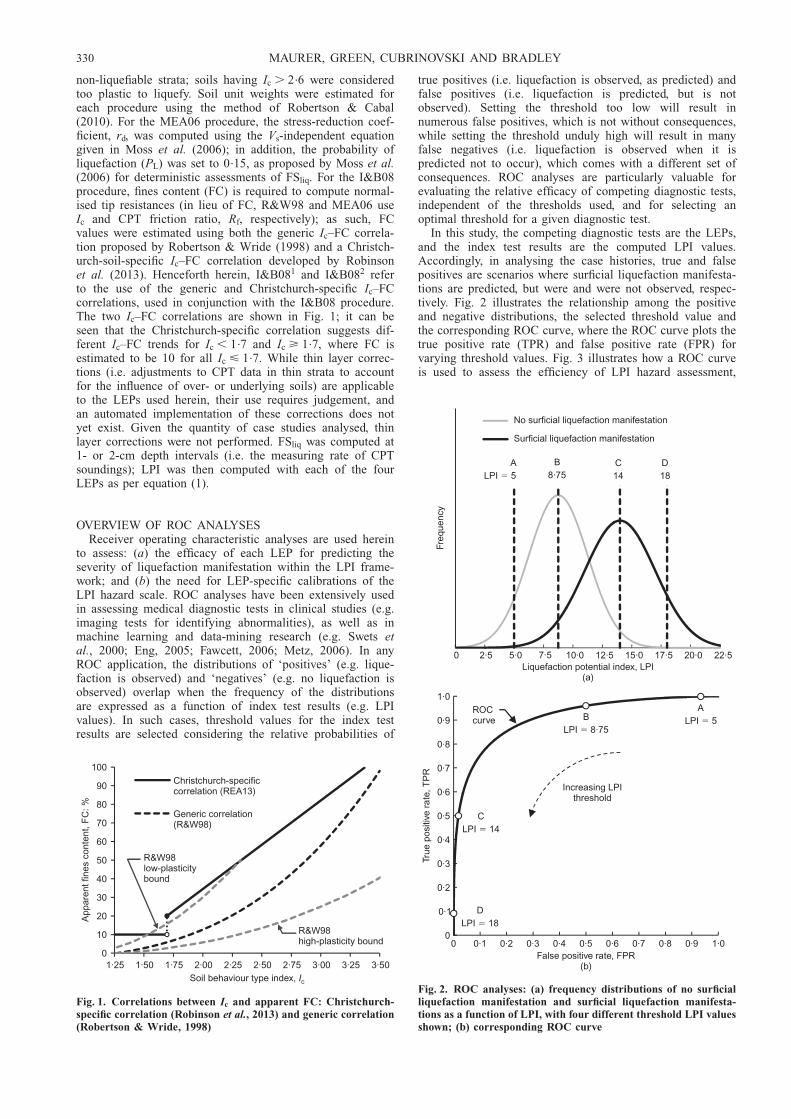
non-liquefiable strata; soils having Ic . 2.6 were consideredtoo plastic to liquefy. Soil unit weights were estimated foreach procedure using the method of Robertson & Cabal(2010). For the MEA06 procedure, the stress-reduction coef-ficient, rd, was computed using the Vs-independent equationgiven in Moss et al. (2006); in addition, the probability ofliquefaction (PL) was set to 0.15, as proposed by Moss et al.(2006) for deterministic assessments of FSliq. For the I&B08procedure, fines content (FC) is required to compute normal-ised tip resistances (in lieu of FC, R&W98 and MEA06 useIc and CPT friction ratio, Rf, respectively); as such, FCvalues were estimated using both the generic Ic–FC correla-tion proposed by Robertson & Wride (1998) and a Christch-urch-soil-specific Ic–FC correlation developed by Robinsonet al. (2013). Henceforth herein, I&B081 and I&B082 referto the use of the generic and Christchurch-specific Ic–FCcorrelations, used in conjunction with the I&B08 procedure.The two Ic–FC correlations are shown in Fig. 1; it can beseen that the Christchurch-specific correlation suggests dif-ferent Ic–FC trends for Ic , 1.7 and Ic > 1.7, where FC isestimated to be 10 for all Ic < 1.7. While thin layer correc-tions (i.e. adjustments to CPT data in thin strata to accountfor the influence of over- or underlying soils) are applicableto the LEPs used herein, their use requires judgement, andan automated implementation of these corrections does notyet exist. Given the quantity of case studies analysed, thinlayer corrections were not performed. FSliq was computed at1- or 2-cm depth intervals (i.e. the measuring rate of CPTsoundings); LPI was then computed with each of the fourLEPs as per equation (1).
OVERVIEW OF ROC ANALYSESReceiver operating characteristic analyses are used herein
to assess: (a) the efficacy of each LEP for predicting theseverity of liquefaction manifestation within the LPI frame-work; and (b) the need for LEP-specific calibrations of theLPI hazard scale. ROC analyses have been extensively usedin assessing medical diagnostic tests in clinical studies (e.g.imaging tests for identifying abnormalities), as well as inmachine learning and data-mining research (e.g. Swets etal., 2000; Eng, 2005; Fawcett, 2006; Metz, 2006). In anyROC application, the distributions of ‘positives’ (e.g. lique-faction is observed) and ‘negatives’ (e.g. no liquefaction isobserved) overlap when the frequency of the distributionsare expressed as a function of index test results (e.g. LPIvalues). In such cases, threshold values for the index testresults are selected considering the relative probabilities of
true positives (i.e. liquefaction is observed, as predicted) andfalse positives (i.e. liquefaction is predicted, but is notobserved). Setting the threshold too low will result innumerous false positives, which is not without consequences,while setting the threshold unduly high will result in manyfalse negatives (i.e. liquefaction is observed when it ispredicted not to occur), which comes with a different set ofconsequences. ROC analyses are particularly valuable forevaluating the relative efficacy of competing diagnostic tests,independent of the thresholds used, and for selecting anoptimal threshold for a given diagnostic test.
In this study, the competing diagnostic tests are the LEPs,and the index test results are the computed LPI values.Accordingly, in analysing the case histories, true and falsepositives are scenarios where surficial liquefaction manifesta-tions are predicted, but were and were not observed, respec-tively. Fig. 2 illustrates the relationship among the positiveand negative distributions, the selected threshold value andthe corresponding ROC curve, where the ROC curve plots thetrue positive rate (TPR) and false positive rate (FPR) forvarying threshold values. Fig. 3 illustrates how a ROC curveis used to assess the efficiency of LPI hazard assessment,
0
10
20
30
40
50
60
70
80
90
100
1·25 1·50 1·75 2·00 2·25 2·50 2·75 3·00 3·25 3·50
App
aren
t fin
es c
onte
nt, F
C: %
Soil behaviour type index, Ic
Christchurch-specificcorrelation (REA13)
Generic correlation(R&W98)
R&W98high-plasticity bound
R&W98low-plasticitybound
Fig. 1. Correlations between Ic and apparent FC: Christchurch-specific correlation (Robinson et al., 2013) and generic correlation(Robertson & Wride, 1998)
0
0·1
0·2
0·3
0·4
0·5
0·6
0·7
0·8
0·9
1·0
0 0·1 0·2 0·3 0·4 0·5 0·6 0·7 0·8 0·9 1·0
True
pos
itive
ra
te, T
PR
False positive rate, FPR(b)
BLPI 8·75�
ALPI 5�
CLPI 14�
DLPI 18�
ROCcurve
Increasing LPIthreshold
0 2·5 5·0 7·5 10·0 12·5 15·0 17·5 20·0 22·5
Freq
uenc
y
Liquefaction potential index, LPI(a)
No surficial liquefaction manifestation
Surficial liquefaction manifestation
ALPI 5�
B8·75
C14
D18
Fig. 2. ROC analyses: (a) frequency distributions of no surficialliquefaction manifestation and surficial liquefaction manifesta-tions as a function of LPI, with four different threshold LPI valuesshown; (b) corresponding ROC curve
330 MAURER, GREEN, CUBRINOVSKI AND BRADLEY

where TPR and FPR are synonymous with ‘true positiveprobability’ and ‘false positive probability’, respectively. InROC curve space, random guessing is indicated by a 1:1 linethrough the origin (i.e. equivalent correct and incorrect pre-dictions), while a perfect model plots as a point at (0,1),indicating the existence of a threshold value which perfectlysegregates the dataset (e.g. all sites with manifestation haveLPI above the selected threshold; all sites without manifesta-tion have LPI below the same selected threshold). While nosingle parameter can fully characterise model performance,the area under a ROC curve (AUC) is commonly used for thispurpose, where AUC is equivalent to the probability that siteswith manifestation have higher computed LPI than sites with-out manifestation (e.g. Fawcett, 2006). As such, increasingAUC indicates better model performance. The optimum oper-ating point (OOP) is defined herein as the threshold LPI valuewhich minimises the rate of misprediction (i.e. FPR + (1 �TPR), where TPR and FPR are the rates of true and falsepositives, respectively). As such, contours of the quantity[FPR + (1 � TPR)] represent points of equivalent perform-ance in ROC space. Thus, in plotting the LPI data as ROCcurves for each LEP, it is possible to assess both the influenceof LEPs on the accuracy of hazard assessments, and the needfor LEP-specific calibrations of the LPI hazard scale.
RESULTS AND DISCUSSIONUtilising more than 7000 combined case studies from the
Darfield and Christchurch earthquakes, LPI values werecomputed using the LEPs of R&W98, MEA06, I&B081 andI&B082.
Prediction of liquefaction occurrenceIn Fig. 4, ROC curves are plotted to evaluate the perform-
ance of each LPI model in segregating sites with and with-out liquefaction manifestation; this initial analysis assessesonly whether LPI accurately predicts the occurrence ofmanifestations and does not yet consider manifestation se-verity. Included in Fig. 4 are data from both the Darfieldand Christchurch earthquakes for all investigation sites,except for those where lateral spreading was the predomi-nant manifestation (the separate assessment of lateral spread-
ing is discussed later in this paper). It can be seen in Fig. 4that, while the four LPI models perform similarly, MEA06and I&B081 are respectively the least and most efficacious,with AUC ranging from 0.71 (MEA06) to 0.78 (I&B081).To place this performance in context, AUCs of 0.5 and 1.0,respectively, indicate random guessing and a perfect model.Also, as highlighted in Fig. 4, the optimum threshold LPIvalues for the R&W98, MEA06, I&B081 and I&B082 mod-els are 4.0, 5.5, 6.0 and 4.5, respectively. Thus, while thelower Iwasaki criterion (i.e. LPI ¼ 5) is generally appropriatefor predicting liquefaction manifestation in Christchurch, theoptimum threshold is LEP dependent. The presence of dif-ferent optimum threshold LPI values for each LEP is notsurprising given that different LEPs have been shown tocommonly compute notably different FSliq values for thesame soil profile (e.g. Green et al., 2014). Although notunexpected, these findings may have important implicationsfor liquefaction hazard assessment, as the risks correspond-ing to particular LPI values depend on the LEP used tocompute LPI.
Also of interest is the influence of the Ic–FC correlationused within the I&B08 LEP. As shown in Fig. 1, theChristchurch-specific correlation infers a higher FC thandoes the generic correlation for all values of Ic, resulting inhigher computed FSliq values, and thus lower computed LPI.As a result, the LPI hazard scale computed using I&B082
(i.e. using the Christchurch-specific correlation) is shiftedtowards lower values relative to the hazard scale computedusing I&B081 (i.e. using the generic correlation) such thatthe median LPI values computed using I&B081 and I&B082
are 7.2 and 4.1, respectively. In addition to influencing theLPI hazard scale, the Ic–FC correlation affects model effi-cacy (i.e. efficiency segregating sites with and withoutliquefaction manifestations), with I&B081 correctly classify-ing 3% more cases than I&B082 when operating at theirrespective OOPs. The slightly weaker performance ofI&B082 might be due to the fact that the Robinson et al.(2013) Christchurch-specific Ic–FC correlation was devel-oped using data from along the Avon River only, while thedatabase assessed herein consists of sites distributed through-out Christchurch, although further analysis is needed toevaluate this hypothesis. As research continues in Christ-church, refined region-specific Ic–FC correlations, which
Improving
performance
Rando
mgu
ess
0
0·1
0·2
0·3
0·4
0·5
0·6
0·7
0·8
0·9
1·0
0 0·1 0·2 0·3 0·4 0·5 0·6 0·7 0·8 0·9 1·0
True
pos
itive
ra
te, T
PR
False positive rate, FPR
Per
fect
mod
el
Perfect model
ROCcurve
OOP
Fig. 3. Illustration of how a ROC curve is used to assess theefficiency of a diagnostic test. The optimum operating point(OOP) indicates the threshold value for which the mispredictionrate is minimised, as described in the text
Iso-p
erform
ancelin
e
0·60
0·65
0·70
0·75
0·80
0·20 0·25 0·30 0·35 0·40
4·0
6·0
5·5
4·5
0
0·1
0·2
0·3
0·4
0·5
0·6
0·7
0·8
0·9
1·0
0 0·1 0·2 0·3 0·4 0·5 0·6 0·7 0·8 0·9 1·0
True
pos
itive
ra
te, T
PR
False positive rate, FPR
R&W98
MEA06
I&B081
I&B082
See insetfigure
Fig. 4. ROC analysis of LPI model performance in predicting theoccurrence of surficial liquefaction manifestation. The optimumthreshold LPI values (i.e. OOPs) for each LEP are highlighted inthe inset figure
ASSESSMENT OF CPT-BASED METHODS FOR LIQUEFACTION EVALUATION 331

might improve the efficacy of LPI hazard assessment inChristchurch, are likely to be developed.
While the preceding ROC analysis showed that optimumthreshold LPI values are LEP dependent, the implications forliquefaction hazard assessment are not intuitively clear. Forexample, it was shown that for the considered dataset theR&W98 and I&B081 LPI models have optimum thresholdLPI values of 4.0 and 6.0, respectively, but the potentialconsequence of failing to account for different optimumthresholds is not easily discerned. To elucidate the signifi-cance of these differences, the probability of surficial lique-faction manifestation is computed herein using the Wilson(1927) interval for a binomial proportion. This assessmentalso allows for application to risk-based frameworks, com-plementing the prior evaluation of deterministic thresholdvalues. The resulting probabilities are plotted in Fig. 5 whereeach data point represents one-twentieth of the correspondingdataset (,350 case histories) and is plotted as a function ofthe median-percentile for each data bin (i.e. 2.5th-percentile,7.5th-percentile, and so on); also shown are third-order poly-nomial regressions for each LPI model. It can be seen fromthese regressions that, at an LPI value of 5.0, the probabil-ities of liquefaction manifestation corresponding to theI&B081, MEA06, R&W98 and I&B082 LPI models are 0.44,0.53, 0.58 and 0.58, respectively. Conversely, using theoptimum threshold LPI values found previously, the prob-abilities corresponding to the respective LPI models are0.50, 0.55, 0.53 and 0.55. Thus, the optimum thresholdscorrespond to roughly the same probability of manifestation,whereas failing to account for the influence of the LEP could
result in different risk levels for the same LPI value,particularly with I&B081.
Prediction of liquefaction severityWhile prediction of the occurrence of surficial manifesta-
tion is an important component of liquefaction hazard analy-sis, the severity of manifestation is of greater consequenceto the built environment and is thus of added importance forhazard mapping and engineering design. To investigate thecapacity of each LPI model for predicting manifestationseverity, additional ROC analyses were performed for eachclassification of severity in Table 1; the results are sum-marised in Table 2 in the form of AUC and recommendedthreshold LPI values. Where the prior ROC analysis assessedeach model’s capacity for predicting any surficial manifesta-tion (i.e. having at least marginal severity), the additionalanalyses assess their ability to predict that manifestationswill be of a particular severity (e.g. moderate as opposed tomarginal). As mentioned previously, lateral spreading istreated separately in this study, and the ‘marginal’, ‘moder-ate’ and ‘severe’ classifications refer only to sand-blowmanifestations. This distinction is made because lateralspreading is a unique manifestation associated with largepermanent ground displacements, and because there areseparate criteria for assessing its severity (e.g. Youd et al.,2002), including the ground slope and height of the nearestfree face (e.g. river bank), among others. Consequently,although site profiles with thin liquefiable layers may havelow LPI values, these sites are susceptible to lateral spread-ing if located on sloping ground or near rivers. Since thefactors pertinent to lateral spreading cases are not consideredin the formulation of LPI, such cases should not be used toassess its performance.
From Table 2, the following observations are made.
(a) Relative trends in model performance, as suggested byAUC, are consistent for each classification of manifesta-tion severity. While the LPI models perform similarly, theI&B081 and MEA06 models are consistently the mostand least efficacious, respectively.
(b) Unsurprisingly, the models are more efficient in predict-ing the incidence of liquefaction manifestation than inpredicting the severity of manifestation (e.g. distinguish-ing between marginal and moderate manifestations);nonetheless, the expected severity of manifestationincreases with increasing LPI.
(c) Differences in optimum threshold LPI values extendthroughout the LPI hazard scale, indicating that the utilityof the Iwasaki criterion varies among LEPs.
(d ) Considering the potential for damage to infrastructure,lateral spreading manifestations have relatively lowoptimum threshold LPI values. For example, lateral
0
0·1
0·2
0·3
0·4
0·5
0·6
0·7
0·8
0·9
1·0
0 5 10 15 20
Pro
babi
lity
ofliq
uefa
ctio
n m
anife
sta
tion
LPI
R&W98
MEA06
I&B081
I&B082
R&W98 ( 0·99)R2 �
I&B08 ( 0·99)2 2R �
I&B08 ( 0·99)1 2R �
MEA06( 0·98)R2 �
�1σ
Fig. 5. Probability of liquefaction manifestation
Table 2. Summary of receiver operator characteristic (ROC) analyses�
LPI Model Allmanifestations†
Marginalmanifestation†
Moderatemanifestation†
Severemanifestation†
Lateralspreading
Severe lateralspreading
OOP‡ AUC§ OOP‡ AUC§ OOP‡ AUC§ OOP‡ AUC§ OOP‡ AUC§ OOP‡ AUC§
R&W98 4.0 0.73 3.0 0.68 5.5 0.62 10.5 0.69 4.5 0.83 10.0 0.66MEA06 5.5 0.71 5.0 0.66 7.5 0.60 14.0 0.68 5.0 0.83 12.0 0.64I&B081 6.0 0.78 5.0 0.72 9.0 0.64 16.0 0.69 6.5 0.79 8.0 0.62I&B082 4.5 0.75 3.0 0.70 6.0 0.63 11.0 0.69 5.0 0.86 8.0 0.63
� Where manifestation severity is characterised as described in Table 1.† Excludes sites where lateral spreading was the predominant manifestation, as described in text.‡ Optimum operating point: recommended optimum threshold LPI value found from ROC analysis.§ Area under ROC curve: general index of model efficacy, where higher AUC indicates better performance.
332 MAURER, GREEN, CUBRINOVSKI AND BRADLEY

spreading and marginal sand-blow manifestations havesimilar OOPs for each respective LPI model (i.e. similarLPI distributions), but the potential for damage toinfrastructure is generally much greater with lateralspreading. This illustrates that while LPI may be usefulfor hazard assessment, the influence of local conditionson the manifestation of liquefaction must also beconsidered. As such, the damage potential of lateralspreading may not be well estimated by LPI.
As was done previously, the probability of manifestationis computed to assess the significance of different optimumthresholds, and to allow for application to risk-based frame-works. Because damage to infrastructure (e.g. settlement ofstructures, failure of lifelines and cracking of pavements) ismore likely a consequence of moderate or severe liquefac-tion, these cases are used to compute the likelihood ofdamaging liquefaction due to sand blows, where marginalliquefaction is considered non-damaging. Using the method-ology previously discussed, the probability of moderate orsevere liquefaction is plotted in Fig. 6 along with third-orderpolynomial regressions for each LPI model. It can be seenfrom these regressions that, at an LPI value of 15.0 (i.e. theupper Iwasaki criterion), the probabilities corresponding tothe I&B081, MEA06, R&W98 and I&B082 LPI models are0.37, 0.40, 0.43 and 0.47, respectively. Conversely, using thethreshold LPI values found previously for severe liquefaction(Table 2), the probabilities corresponding to the respectiveLPI models are 0.39, 0.39, 0.38 and 0.40. Thus, theoptimum thresholds correspond to roughly the same prob-ability of damaging manifestation, whereas failing to accountfor the influence of the LEP results in different risk levels.Similarly, the optimum thresholds for moderate liquefactioncorrespond to the same level of risk (,27%).
Comparative performance in an applied frameworkThe preceding analyses have suggested the four LPI
models may be capable of assessing liquefaction hazard, butthat LEP-specific correlations relating LPI values and sever-ity of surficial liquefaction manifestations are required. Tocompare LEP performance in an applied setting, and todetermine whether any LEP is superior for practical intentsand purposes, deterministic ‘prediction errors’ are computedfor each case history using both the Iwasaki criterion and
the LEP-specific calibrations in Table 2. The prediction error(E) is computed using the thresholds assigned to eachmanifestation category, such that E ¼ LPI � (min or max) ofthe relevant range. For example, using the Iwasaki criterion,if the computed LPI is 14 for a site with no manifestation,E ¼ 14 � 5 ¼ 9 (where 5 is the maximum of the range ofLPI values for no manifestation), whereas if the computedLPI is 6 for a site with severe liquefaction, E ¼ 6 � 15 ¼�9 (where 15 is the minimum of the range of LPI valuesfor severe liquefaction). Thus, positive errors indicate over-predictions of manifestation severity and, conversely, nega-tive errors indicate under-predictions. While there is noprecedent for using a ‘moderate manifestation’ thresholdwith the Iwasaki criterion, an LPI value of 8.0 is used hereinto facilitate comparisons among the models. Also, in light ofthe separate criteria for assessing lateral spreads, lateralspreading is assigned a wide range of expected LPI valuesconsistent with any manifestation, independent of spreadingseverity (i.e. lateral spread sites are only expected to haveLPI > the threshold for marginal liquefaction).
The distributions of LPI prediction errors are shown foreach model in Fig. 7 using both the Iwasaki (Fig. 7(a)) andLEP-specific (Fig. 7(b)) hazard scales. It can be seen in Fig.7(a) that the distributions of errors among LEPs vary usingthe Iwasaki criterion, as expected. Because the models havedifferent LPI hazard scales, applying the Iwasaki criterion toeach results in dissimilar performance. For example,R&W98 and I&B081 under-predict manifestation severity for38% and 18% of cases, respectively. Conversely, using the
0
0·1
0·2
0·3
0·4
0·5
0·6
0 5 10 15 20
Pro
babi
lity
ofm
oder
ate
or
seve
re m
anife
sta
tion
LPI
R&W98
MEA06
I&B081
I&B082
R&W98 ( 0·98)R2 �
I&B08 ( 0·99)2 2R �
I&B08 ( 0·98)1 2R �
MEA06 ( 0·97)R2 �
�1σ
Fig. 6. Probability of moderate or severe liquefaction manifesta-tion
0
5
10
15
20
25
30
35
40
45
50
�25 �20 �15 �10 �5 0 5 10 15 20 25
Pre
dict
ion
rate
(72
32 c
ases
): %
Prediction error: LPI units(a)
R&W98
MEA06
I&B081
I&B082
35%
40%
45%
�0·2 0 0·2
0
5
10
15
20
25
30
35
40
45
50
�25 �20 �15 �10 �5 0 5 10 15 20 25
Pre
dict
ion
rate
(72
32 c
ases
): %
Prediction error: LPI units(b)
R&W98
MEA06
I&B081
I&B082
35%
40%
45%
�0·2 0 0·2
Fig. 7. Distribution of LPI prediction errors, computed from theLPI hazard scales defined by: (a) the Iwasaki criterion; (b) LEP-specific calibrations given in Table 2
ASSESSMENT OF CPT-BASED METHODS FOR LIQUEFACTION EVALUATION 333

LEP-specific calibrations of the LPI hazard scale (Fig. 7(b)),the distributions of errors among LEPs are more similar. Forexample, R&W98 and I&B081 under-predict manifestationseverity for 24% and 20% of cases, respectively. In addition,the rate of accurate prediction (i.e. zero error) is improvedfor each LEP; R&W98, MEA06, I&B081 and I&B082
accurately predict 44%, 42%, 46% and 44% of cases, re-spectively. These performance trends mirror those of theROC analyses, which indicated that, although the modelsperformed similarly, I&B081 and MEA06 were respectivelythe most and least efficacious. However, although accuratepredictions of manifestation severity are important, so too islimiting the rate of highly erroneous predictions, which arenot necessarily mutually inclusive. While I&B081 has themost zero-error predictions (46%), it also has the mostpredictions with |E| . 15 (5%). Conversely, MEA06 has theleast zero-error predictions (42%), but it also has the fewestpredictions with |E| . 15 (2.5%). Given these inconsisten-cies, and considering the variety of metrics that might beused to gauge performance, it is difficult to argue that anyone LEP is superior in this applied framework. Thus, usingthe LEP-specific hazard scales, and based on the predictionerrors computed herein, the performance of the LPI modelsis, for practical intents and purposes, equivalent.
While minor errors are to be expected in any deterministicanalysis, each model produced significant errors with con-sequences for hazard assessment. For example, even withcalibration, |E| exceeded 10 at 9% of sites, on average, foreach model (e.g. severe manifestation predicted, but nomanifestation observed) and |E| exceeded 5 at 22% of sites,on average, for each model (e.g. no manifestation predicted,but moderate manifestation observed). To determine whethercertain models perform better in particular locations, predic-tion errors from the calibrated R&W98, MEA06 andI&B082 models are plotted against one another in Fig. 8. Itcan be seen that prediction errors are generally equivalent;in all, the difference in prediction error between any two ofthe models exceeds �5 for only 12% of investigation sites.Thus, locations of under-, over- and accurate prediction aregenerally consistent between models. In addition, mapsshowing the spatial distributions of errors to be very similarin both earthquakes are provided in an electronic supplementto this paper. Thus, some site profiles have very poorpredictions, irrespective of the LEP used (note that Maureret al. (2014) found no correlation between prediction errorsand either PGA uncertainty, ground water fluctuation or CPTtermination depth). This suggests that LPI has inherentlimitations in its formulation, such that the variables influ-encing surficial manifestation are not adequately accountedfor. While liquefaction triggering has garnered significantresearch and is a subject of frequent debate, the mechanicsof liquefaction manifestation have received less attention.This study highlights that triggering and manifestation aretwo distinct phenomena contributing to liquefaction hazard,and that an improved framework providing clear separationand accounting of the two phenomena is needed.
Lastly, the 12% of cases with inconsistent predictionerrors between models can be shown to correspond to‘exceptional’ site profiles. Since the LEP-specific calibrationsare based on the entire dataset (i.e. predominant behaviouracross Christchurch), predictions for site profiles that divergefrom typical conditions may be inconsistent among models.As an example, it can be seen in Figs 8(a) and 8(c) that anumber of cases exist where the MEA06 prediction errorsignificantly differs from that of R&W98 and I&B082. Onecommon cause of this discrepancy is cases where relativelythick, potentially liquefiable layers are present at depthsgreater than ,10 m. For such cases the LEPs can yielddivergent FSliq and hence divergent LPI values. However, the
LEP-specific calibrations do not account for this divergencebecause the median cumulative thickness of soil stratapredicted to liquefy below 10 m depth for all the sites in thedataset is only 0.35 m, according to I&B082. This empha-sises that assessments and/or calibrations of the LPI hazardscale are a function not only of the selected LEP, but also ofthe chosen dataset, including the geometry and soil charac-teristics of site profiles, as well as the amplitude and dura-tion of ground shaking. As such, the applicability of findingsderived herein to other datasets is unknown.
�15
�5
5
15
25
35
ME
A06
pre
dict
ion
erro
r: L
PI u
nits
Christchurch
Darfield
| | 5E �
�15 �5 5 15 25 35MEA06 prediction error: LPI units
(a)
�15
�5
5
15
25
35
I&B
08pr
edic
tion
erro
r: L
PI u
nits
2
Christchurch
Darfield
�15 �5 5 15 25 35MEA06 prediction error: LPI units
(b)
�15
�5
5
15
25
35
�15 �5 5 15 25 35
I&B
08pr
edic
tion
erro
r: L
PI u
nits
2
MEA06 prediction error: LPI units(c)
Christchurch
Darfield
Fig. 8. Comparison of LPI model prediction errors at eachinvestigation site, as computed by: (a) R&W98 plotted againstMEA06; (b) R&W98 plotted against I&B082; (c) MEA06 plottedagainst I&B082
334 MAURER, GREEN, CUBRINOVSKI AND BRADLEY

SUMMARY AND CONCLUSIONSUtilising high-quality case histories from the CES, this
study evaluated the performance of the R&W98, MEA06,I&B081 and I&B082 CPT-based LEPs, operating within theLPI framework, for assessing liquefaction hazard. The find-ings are summarised as follows.
(a) For deterministic analyses, the optimum threshold LPIvalues for assessing liquefaction hazard were unique tothe LEP used in the LPI framework; suggested optimumthresholds for the CES dataset are summarised in Table 2.The use of LPI for assessing lateral spread potential is notrecommended.
(b) Taking these LEP-specific threshold values into account,receiver-operating-characteristic analyses indicated that,while the models performed similarly, the I&B081 andMEA06 models were respectively the most and leastefficacious.
(c) LPI probability curves were computed to assess thesignificance of different optimum thresholds, and to allowfor application in probabilistic frameworks. The optimumthresholds were shown to correspond to roughly the sameprobability of manifestation, whereas failing to accountfor the influence of the LEP (i.e. using the Iwasakicriterion) resulted in different risk levels for the same LPIvalue.
(d ) To compare model performance in a practical setting,deterministic ‘prediction errors’ were computed for eachcase history. Using the Iwasaki criterion, the distributionsof errors among LEPs varied. These distributions becamemore similar using the LEP-specific hazard scales givenin Table 2, which also improved the rate of accurateprediction for all LEPs.
(e) Even with calibration, each model had significantprediction errors (e.g. severe manifestation predicted,but no manifestation observed). This suggests that LPIhas inherent limitations in its formulation, such that thevariables influencing surficial liquefaction manifestationare not adequately accounted for.
( f ) The findings presented in this study are based on a datasetfrom the CES; the applicability of these findings to otherdatasets is unknown.
In conclusion, the following points can be made.
(a) The risk levels corresponding to the Iwasaki criterionvaried among LEPs.
(b) Using a calibrated, LEP-specific hazard scale, theperformance of the LPI models was, for practical intentsand purposes, equivalent.
(c) The existing LPI framework has inherent limitations suchthat all LEPs have very poor predictions for certain soilprofiles. It is unlikely that revisions of the LEPs willcompletely resolve these erroneous assessments. Rather,a revised index which more adequately accounts for themechanics of liquefaction manifestation is needed.
ACKNOWLEDGEMENTSThis study is based on work supported by the US National
Science Foundation (NSF) grants CMMI 1030564, CMMI1407428 and CMMI 1435494 and US Army EngineerResearch and Development Center (ERDC) grant W912HZ-13-C-0035. The third and fourth authors would like toacknowledge the continuous financial support provided bythe Earthquake Commission (EQC) and Natural HazardsResearch Platform (NHRP), New Zealand, for the researchand investigations related to the 2010–2011 Canterburyearthquakes. The authors also acknowledge the New ZealandGeoNet project and its sponsors EQC, GNS Science and
Land Information New Zealand (LINZ) for providing theearthquake occurrence data and the Canterbury GeotechnicalDatabase and its sponsor EQC for providing the CPT sound-ings, lateral spread observations and aerial imagery used inthis study. However, any opinions, findings, and conclusionsor recommendations expressed in this paper are those of theauthors and do not necessarily reflect the views of NSF,ERDC, EQC, NHRP or LINZ.
SUPPLEMENTAL DATAThe following are available in an electronic supplement:
(a) aerial images representative of the liquefaction manifes-tation severity classes described in Table 1; and (b) mapfigures showing the spatial distribution of LPI predictionerrors for each LPI model, for both the Darfield andChristchurch earthquakes.
NOTESome of the data used in this study were extracted from
the Canterbury Geotechnical Database (https://canterburygeotechnicaldatabase.projectorbit.com), which was preparedand/or compiled for the Earthquake Commission (EQC) toassist in assessing insurance claims made under the Earth-quake Commission Act 1993 and/or for the CanterburyGeotechnical Database on behalf of the Canterbury Earth-quake Recovery Authority (CERA). The source maps anddata were not intended for any other purpose. EQC, CERAand their data suppliers, and their engineers, Tonkin &Taylor, have no liability for any use of these maps and dataor for the consequences of any person relying on them inany way.
NOTATIONIc soil behaviour type index
PL probability of liquefactionRf cone penetration test friction ratiord stress reduction coefficientVs shear wave velocity
w(z) depth weighting function given by w(z) ¼ 10 � 0.5zz depth below ground surface (m)� standard deviation
REFERENCESAnselin, L. (1995). Local indicators of spatial association – LISA.
Geographical Anal. 27, No. 2, 93–115.Baise, L. G., Higgins, R. B. & Brankman, C. M. (2006). Liquefac-
tion hazard mapping-statistical and spatial characterization ofsusceptible units. J. Geotech. Geoenviron. Engng 132, No. 6,705–715.
Bradley, B. A. & Cubrinovski, M. (2011). Near-source strongground motions observed in the 22 February 2011 Christchurchearthquake. Seismol. Res. Lett. 82, No. 6, 853–865.
Bradley, B. A. (2013a). Estimation of site-specific and spatially-distributed ground motion in the Christchurch earthquakes: Ap-plication to liquefaction evaluation and ground motion selectionfor post-event investigation. Proceedings of the 19th New Zeal-and geotechnical symposium, Queenstown, New Zealand, p. 8.
Bradley, B. A. (2013b). A New Zealand-specific pseudo-spectralacceleration ground-motion prediction equation for active shal-low crustal earthquakes based on foreign models. Bull. Seismol.Soc. Am. 103, No. 3, 1801–1822.
CGD (Canterbury Geotechnical Database) (2012a). Geotechnicalinvestigation data. Map layer CGD0010. See https://canterburygeotechnicaldatabase.projectorbit.com (accessed 12/01/2012).
CGD (2012b). Aerial photography. Map layer CGD0010. Seehttps://canterburygeotechnicaldatabase.projectorbit.com (accessed12/01/2012).
Chung, J. & Rogers, J. (2011). Simplified method for spatial
ASSESSMENT OF CPT-BASED METHODS FOR LIQUEFACTION EVALUATION 335

evaluation of liquefaction potential in the St. Louis Area.J. Geotech. Geoenviron. Engng 137, No. 5, 505–515.
Cramer, C. H., Rix, G. J. & Tucker, K. (2008). Probabilisticliquefaction hazard maps for Memphis, Tennessee. Seismol. Res.Lett. 79, No. 3, 416–423.
Cubrinovski, M. & Green, R. A. (2010). Geotechnical reconnais-sance of the 2010 Darfield (Canterbury) earthquake. Bull. NewZealand Soc. Earthquake Engng 43, No. 4, 243–320.
Cubrinovski, M., Bradley, B., Wotherspoon, L., Green, R., Bray, J.,Woods, C., Pender, M., Allen, J., Bradshaw, A., Rix, G., Taylor, M.,Robinson, K., Henderson, D., Giorgini, S., Ma, K., Winkley, A.,Zupan, J., O’Rourke, T., DePascale, G. & Wells, D. (2011). Geo-technical aspects of the 22 February 2011 Christchurch earthquake.Bull. New Zealand Soc. Earthquake Engng 43, No. 4, 205–226.
Eng, J. (2005). Receiver operating characteristic analysis. AcademicRadiol. 12, No. 12, 909–916.
Fawcett, T. (2006). An introduction to ROC analysis. PatternRecognition Lett. 27, No. 8, 861–874.
Green, R. A., Allen, A., Wotherspoon, L., Cubrinovski, M., Bradley,B., Bradshaw, A., Cox, B. & Algie, T. (2011). Performance oflevees (stopbanks) during the 4 September Mw7.1 Darfield and22 February 2011 Mw6.2 Christchurch, New Zealand, earth-quakes. Seismol. Res. Lett. 82, No. 6, 939–949.
Green, R. A., Cubrinovski, M., Cox, B., Wood, C., Wotherspoon,L., Bradley, B. & Maurer, B. (2014). Select liquefaction casehistories from the 2010–2011 Canterbury earthquake sequence.Earthquake Spectra 30, No. 1, 131–153.
Hayati, H. & Andrus, R. D. (2008). Liquefaction potential map ofCharleston, South Carolina based on the 1986 earthquake.J. Geotech. Geoenviron. Engng 134, No. 6, 815–828.
Holzer, T. L. (2008). Probabilistic liquefaction hazard mapping. InGeotechnical Earthquake Engineering and Soil Dynamics IV,ASCE Geotechnical Special Publication 181 (eds D. Zeng,M. T. Manzari and D. R. Hiltunen). Reston, VA, USA: Amer-ican Society of Civil Engineers.
Holzer, T. L., Bennett, M. J., Noce, T. E., Padovani, A. C. &Tinsley, J. C. III. (2006a). Liquefaction hazard mapping withLPI in the greater Oakland, California area. Earthquake Spectra22, No. 3, 693–708.
Holzer, T. L., Blair, J. L., Noce, T. E. & Bennett, M. J. (2006b).LIQUEMAP: A real-time post-earthquake map of liquefactionprobability. Proceedings of the 8th U. S. national conference onearthquake engineering (100th anniversary earthquake confer-ence), paper no. 89. Oakland, CA, USA: Earthquake Engineer-ing Research Institute (CD-ROM).
Idriss, I. M. & Boulanger, R. W. (2008). Soil liquefaction duringearthquakes, Monograph MNO-12, p. 261. Oakland, CA, USA:Earthquake Engineering Research Institute.
Iwasaki, T., Tatsuoka, F., Tokida, K. & Yasuda, S. (1978). Apractical method for assessing soil liquefaction potential basedon case studies at various sites in Japan. Proceedings of the 2ndinternational conference on microzonation for safer construction– research and application, vol. II, pp. 885–896. Arlington, VA,USA: National Science Foundation.
Kang, G. C., Chung, J. W. & Rogers, R. J. (2014). Re-calibratingthe thresholds for the classification of liquefaction potentialindex based on the 2004 Niigata-ken Chuetsu earthquake. EngngGeol. 169, 30–40.
Lenz, A. & Baise, L. G. (2007). Spatial variability of liquefactionpotential in regional mapping using CPT and SPT data. SoilDynam. Earthquake Engng 27, No. 7, 690–702.
Maurer, B. W., Green, R. A., Cubrinovski, M. & Bradley, B. A.(2014). Evaluation of the liquefaction potential index for asses-
sing liquefaction hazard. J. Geotech. Geoenviron. Engng 140,No. 7, 04014032.
Metz, C. E. (2006). Receiver operating characteristic analysis: atool for the quantitative evaluation of observer performance andimaging systems. J. Am. College Radiol. 3, No. 6, 413–422.
Moss, R. E. S., Seed, R. B., Kayen, R. E., Stewart, J. P., DerKiureghian, A. & Cetin, K. O. (2006). CPT-based probabilisticand deterministic assessment of in situ seismic soil liquefactionpotential. J. Geotech. Geoenviron. Engng 132, No. 8, 1032–1051.
Murahidy, K. M., Soutar, C. M., Phillips, R. A. & Fairclough, A.(2012). Post earthquake recovery – development of a geotechni-cal database for Christchurch central city. Proceedings of the15th world conference on earthquake engineering, Lisbon, Por-tugal. Tokyo, Japan: International Association of EarthquakeEngineering.
Papathanassiou, G. (2008). LPI-based approach for calibrating theseverity of liquefaction-induced failures and for assessing theprobability of liquefaction surface evidence. Engng Geol. 96,No. 1–2, 94–104.
Quigley, M., Bastin, S. & Bradley, B. (2013). Recurrent liquefactionin Christchurch, New Zealand during the Canterbury earthquakesequence. Geology 41, No. 4, 419–422.
Robertson, P. K. & Cabal, K. L. (2010). Estimating soil unit weightfrom CPT. Proceedings of the 2nd international symposium oncone penetration testing, Huntington Beach, CA, USA, paperno. 2, p. 40.
Robertson, P. K. & Wride, C. E. (1998). Evaluating cyclic liquefac-tion potential using cone penetration test. Can. Geotech. J. 35,No. 3, 442–459.
Robinson, K., Cubrinovski, M. & Bradley, B. A. (2013). Sensitivityof predicted liquefaction-induced lateral displacements from the2010 Darfield and 2011 Christchurch Earthquakes. Proceedingsof the New Zealand Society for Earthquake Engineering AnnualConference, Wellington, New Zealand, p. 8.
Seed, H. B. & Idriss, I. M. (1971). Simplified procedure forevaluating soil liquefaction potential. J. Soil Mech. Found. Div.,ASCE 97, No. 9, 1249–1273.
Sonmez, H. (2003). Modification of the liquefaction potential indexand liquefaction susceptibility mapping for a liquefaction-pronearea (Inegol, Turkey). Environ. Geol. 44, No. 7, 862–871.
Swets, J. A., Dawes, R. M. & Monahan, J. (2000). Better decisionsthrough science. Scientific American 283, No. 4, 82–87.
Toprak, S. & Holzer, T. (2003). Liquefaction potential index: fieldassessment. J. Geotech. Geoenviron. Engng 129, No. 4, 315–322.
van Ballegooy, S., Cox, S. C., Thurlow, C., Rutter, H. K., Reynolds,T., Harrington, G., Fraser, J. & Smith, T. (2014). Median watertable elevation in Christchurch and surrounding area after the 4September 2010 Darfield earthquake: Version 2, GNS ScienceReport 2014/18. Lower Hutt, New Zealand: GNS Science.
Whitman, R. V. (1971). Resistance of soil to liquefaction andsettlement. Soils Found. 11, No. 4, 59–68.
Wilson, E. B. (1927). Probable inference, the law of succession,and statistical inference. J. Am. Statistical Assoc. 22, No. 158,209–212.
Youd, T. L., Hansen, C. M. & Bartlett, S. F. (2002). Revisedmultilinear regression equations for prediction of lateral spreaddisplacement. J. Geotech. Geoenviron. Engng 128, No. 12,1007–1017.
Zou, K. H. (2007). Receiver operating characteristic (ROC) litera-ture research. On-line bibliography. See http://www.spl.harvard.edu/archive/spl-pre2007/pages/ppl/zou/roc.html (accessed 15/03/2014).
336 MAURER, GREEN, CUBRINOVSKI AND BRADLEY