Embed Size (px)
Citation preview

ASSESSING THE EFFECTIVE DEMAND FOR IMPROVED
WATER SUPPLY SERVICE IN MALAYSIA: FOCUSING
ON JOHOR WATER COMPANY
Zuraini Anang
A thesis submitted for the degree of Doctor of Philosophy in the
School of Architecture, Planning and Landscape
at
Newcastle University
United Kingdom
January 2013

ii
ABSTRACT
In Malaysia, the water management system was restructured in January 2005 by the
transfer of water supplies and services from the State List to the Concurrent List. The
National Water Services Commission or Suruhanjaya Perkhidmatan Air Negara (SPAN)
was established in July 2006 as the technical and economic regulator for the improvement
of water supply quality and the efficiency of the water industry. This study focuses on
SAJ Holdings (SAJH). This water supply company provides a fully integrated service, i.e.
it is involved in the all the processes of drinking water supply; these range from raw water
acquisition, treatment and purification, and the subsequent distribution of purified water
to customers, plus billing and payment collection.
This study attempts to assess the residential customers‟ preferences of different attributes
of water supply. The water attributes are divided into two categories: Water Infrastructure
(WI) and Residential Customers (RC). WI attributes are leakage, pipe bursts, and
reservoirs; RC attributes are water quality, pressure, connections, and disruptions. Choice
modelling (CM) was applied as a tool for the assessment of effective demand for
improved water supplies, particularly by residential customers. There are two
econometric models employed: Conditional Logit (CL) and Mixed Logit (MXL). Face-to-
face interviews were conducted with residential customers and Statistical Analysis
Software (SAS) was used in order to analyse the data.
The model consists of a basic model and an interaction model with socioeconomic
characteristics. The findings show that the significant variables affecting demand are pipe
bursts, (BUR), water quality (QUA), disruption (DIS) and connection (CON), as well as
price (PRI). Among the socioeconomic characteristics that interact with the main
attributes are gender, age, number of children, type of house, number of persons in the
household, education, work, and income. This information is very useful for the water
provider when upgrading the water service for valuable customers.

iii
ACKNOWLEDGEMENTS
The journey to complete this study involved high commitment and discipline. Therefore,
to achieve the final destination needed full support and assistance from many individuals,
if not this research would have faced many difficulties. The deepest appreciation to all
those who have contributed either directly or indirectly towards completing this research.
First and foremost, I would like to express my sincere gratitude to my supervisor,
Professor Dr Ken Willis, for his excellent guidance and patience, and for providing me
with an excellent atmosphere for doing research; also for his encouragement and support
from the initial to the final level, which enabled me to develop an understanding of this
field. Without his guidance and persistent help this thesis would not have been possible.
Special thanks also to my co-supervisor Dr Graham Tipple for his help and guidance in
completing this study.
I wish to thank SAJ Holdings Sdn. Bhd. and their officers and staff for their involvement,
comments and help regarding this research, and particularly for providing the relevant
data and information required for the completion of this research. Thanks also to my
friends and those who have been involved in the data collection at SAJH.
Many thanks to the Government of Malaysia and University Malaysia Terengganu
(UMT) for granting the scholarship and study leave that enabled this study to take place.
Thanks also to Newcastle University for providing a good environment and facilities to
complete this study.
I would like to express the greatest gratitude to my husband, Nadzruddin Hj Ismail and
my children, Nur MuhammadilKahfi, Nur Muhammad Al Harith, Nur Ainil Fatehah, and
Nur Ehlas Merriyam. They are always supporting me and encouraging me with their best
wishes.
Finally, an honourable mention goes to my extended family and my friends for their
prayers, patience, understanding, encouragement and support in completing this research.

iv
TABLE OF CONTENTS
Page
ABSTRACT ..................................................................................................................... ii
ACKNOWLEDGEMENTS ............................................................................................ iii
TABLE OF CONTENTS ................................................................................................ iv
TABLE OF FIGURES etc. ............................................................................................. xii
LIST OF ABBREVIATIONS ....................................................................................... xvi
LIST OF STATISTICAL VARIABLES USED ........................................................ xviii
CHAPTER 1: INTRODUCTION .....................................................................................1
1.1 Background of Study .............................................................................................1
1.2 Research Questions ...............................................................................................4
1.2.1 Statement of the Problem .............................................................................4
1.3 Research Objectives ..............................................................................................6
1.4 Significance of the Research .................................................................................6
1.5 Overview of the Thesis .........................................................................................7
CHAPTER 2: LITERATURE REVIEW ........................................................................9
2.1 Introduction ...........................................................................................................9
2.2 Review of Non-Market Valuation Methods ..........................................................9
2.2.1 Contingent Valuation Methods (CVM) ........................................................9
2.2.2 Choice Modelling (CM) .............................................................................11
2.3 Choice Experiment for Valuing Water Supply ...................................................17
2.4 Choice Experiment Used in Non-Market Goods ................................................22
2.5 Overview of Economic Valuation in Malaysia ...................................................24
2.6 Factors Affecting WTP for Water Services ........................................................25
2.7 Cost Benefit Analysis for Water Improvement ...................................................29
2.8 Conclusions .........................................................................................................31

v
CHAPTER 3: STUDY DESCRIPTION ........................................................................32
3.1 Introduction .........................................................................................................32
3.2 Background of Study Site ...................................................................................32
3.3 Socioeconomic Characteristics of Study Site......................................................33
3.4 Transformation of Johor Water Supply ...............................................................35
3.5 Water Treatment Process ....................................................................................36
3.6 Water Infrastructure ............................................................................................39
3.6.1 Water Demand ............................................................................................39
3.6.2 Pipelines and Reservoirs ............................................................................39
3.7 Water Tariffs, Revenue and Expenditure ............................................................41
3.8 Water Management, Planning and Monitoring ...................................................42
3.8.1 Setting of Measurable Targets ....................................................................42
3.9 Appraisal of SAJH ..............................................................................................45
3.9.1 Service Quality ...........................................................................................45
3.9.2 Customer Charter .......................................................................................46
3.10 Non-Revenue Water (NRW) ...............................................................................48
3.11 Water Quality ......................................................................................................49
3.12 Network ...............................................................................................................51
3.13 Asset Replacement ..............................................................................................52
3.14 Conclusions .........................................................................................................53
CHAPTER 4: METHODS AND PROCEDURES ........................................................55
4.1 Introduction .........................................................................................................55
4.2 Properties of Discrete Choice Models .................................................................55
4.2.1 Choice Set ..................................................................................................55
4.2.2 Identification of Choice Models .................................................................56
4.2.3 Statistical Significant of Model Estimates .................................................57
4.2.4 Limitations of the MNL Model ..................................................................58
4.2.5 Panel Nature of Data ..................................................................................60

vi
4.2.6 Taste Heterogeneity ....................................................................................60
4.3 Theoretical Framework .......................................................................................61
4.4 The Mixed Logit Model (MXL)..........................................................................64
4.5 Design Stages in the Choice Experiment ............................................................67
4.5.1 Defining Attributes .....................................................................................67
4.5.2 Attribute Levels ..........................................................................................69
4.5.3 Choice Options ...........................................................................................71
4.5.4 Experimental Design ..................................................................................71
4.5.5 Choice Sets .................................................................................................73
4.6 Questionnaire Design ..........................................................................................74
4.6.1 Focus Group ...............................................................................................76
4.7 Fieldwork Data Collection ..................................................................................78
4.7.1 Pilot Test ....................................................................................................78
4.7.2 Data Sources and Techniques of Data Collection ......................................81
4.7.3 Sampling Design ........................................................................................83
4.7.4 Sample Size Requirements .........................................................................84
4.7.5 Justification of Interview Site ....................................................................85
4.8 Conclusions .........................................................................................................87
CHAPTER 5: DESCRIPTIVE ANALYSIS ..................................................................89
5.1 Introduction .........................................................................................................89
5.2 Residential Customers Survey ............................................................................89
5.3 Socioeconomic Profile ........................................................................................90
5.4 Respondents‟ Experience with SAJH .................................................................93
5.5 Perceptions of Service Quality Performance ......................................................95
5.6 Perceptions of Improvement of Service Quality .................................................98
5.7 Perception on Improvement of Strategy............................................................100
5.8 Cross Tabulation Analysis of Perceptions and Socioeconomic Characteristics102
5.8.1 Cross Tabulation Analysis Perceptions of Service Quality Performance and
Socioeconomics ........................................................................................102

vii
5.8.2 Cross Tabulation Analysis Perceptions of Water Service Improvement and
Socioeconomics ........................................................................................106
5.8.3 Cross Tabulation Analysis: Perceptions of Improvement of Strategies and
Socioeconomics ........................................................................................109
5.9 Correlation Analysis of Customers Perception and Socioeconomics ...............111
5.9.1 Correlation Perceptions of Service Quality Performance and
Socioeconomics ........................................................................................111
5.9.2 Correlation Perceptions of Service Factors and Socioeconomics ............121
5.9.3 Correlation Perceptions of Strategies and Socioeconomics.....................129
5.10 Conclusions .......................................................................................................136
CHAPTER 6: CHOICE EXPERIMENT RESULTS .................................................139
6.1 Introduction .......................................................................................................139
6.2 Pattern of Responses .........................................................................................139
6.3 Results for the Basic CL Model ........................................................................142
6.4 Results of the CL Model with Levels Incorporated ..........................................146
6.5 Improving the Model Fit ...................................................................................149
6.5.1 Results of the CL Interaction Model, Choice 1: Water Infrastructure (WI)
..................................................................................................................150
6.5.2 Results of the CL Interaction Model, Choice 2: Residential Customers
(RC) ..........................................................................................................154
6.5.3 Results of the CL Interaction Incorporating Level Model, Choice 1: Water
Infrastructure (WI) ...................................................................................158
6.5.4 Results for the Interaction CL Incorporating Level Model, Choice 2:
Residential Customers (RC) .....................................................................161
6.6 Conclusions .......................................................................................................164
CHAPTER 7: MIXED LOGIT RESULTS .................................................................169
7.1 Introduction .......................................................................................................169
7.2 Results for the Basic MXL Model ....................................................................171
7.3 Results of the MXL Interaction Model, Choice 1: Water Infrastructure (WI) .......
...........................................................................................................................174
7.4 Results of the MXL Interaction Model, Choice 2: Residential Customers (RC)
...........................................................................................................................179

viii
7.5 Conclusions .......................................................................................................182
CHAPTER 8: COST BENEFIT ANALYSIS RESULTS ...........................................185
8.1 Introduction .......................................................................................................185
8.2 Stages of CBA for a Water Supply System ......................................................185
8.3 The Scenario of SAJH .......................................................................................192
8.4 Formula of Cost-Benefit Analysis.....................................................................194
8.5 Implementation of CBA in SAJH .....................................................................195
8.6 Conclusions .......................................................................................................197
CHAPTER 9: IMPLICATIONS OF RESULTS .........................................................198
9.1 Introduction .......................................................................................................198
9.2 Implications of Socioeconomic Characteristics ................................................198
9.3 Implications of Customers‟ Experience with SAJH .........................................199
9.4 Implications of Perceptions of Service Quality.................................................200
9.5 Implications of Perceptions of Improvement of Water Service ........................200
9.6 Implication of the Choice Experiments Results ................................................201
9.7 Policy Implications ............................................................................................201
CHAPTER 10: CONCLUSIONS .................................................................................206
10.1 Introduction .......................................................................................................206
10.2 Summary of the Thesis ......................................................................................206
10.3 Conclusion of the Choice Experiments Study...................................................209
10.4 Potential Improvement Areas ............................................................................213
10.4.1 New Approach of Attributes and Levels ..................................................213
10.4.2 Increase the Number of Attributes ...........................................................213
10.4.3 Increase the Number of Water Operators .................................................213
10.4.4 Improvement of the Questionnaire Design ..............................................214
10.5 Suggestions for Future Research .......................................................................214
10.6 Closing Remarks...............................................................................................215

ix
REFERENCES ...............................................................................................................216
APPENDIX A: QUESTIONNAIRE .............................................................................236
APPENDIX B: CROSS TAB AND CORRELATION ...............................................253
Appendix B1: Cross Tab Water Service Performance and Socioeconomics ..............253
Appendix B2: Cross Tab Service Factor Improvement and Socioeconomics .............264
Appendix B3: Cross Tab Improvement of Strategies and Socioeconomics ................275
Appendix B4 ................................................................................................................281
Appendix B4.1 (a): Correlation of Service Quality Performance with Malay ........281
Appendix B4.1 (b): Correlation of Service Quality Performance with Chinese .....282
Appendix B4.1 (c): Correlation of Service Quality Performance with Indian ........283
Appendix B4.2 (a): Correlation of Service Quality Performance with Age (20 to 30
years old) ..................................................................................................284
Appendix B4.2 (b): Correlation of Service Quality Performance with Age (31 to 40
years old) ..................................................................................................285
Appendix B4.2 (c): Correlation of Service Quality Performance and Age (41 to 50
years old) ..................................................................................................286
Appendix B4.2 (d): Correlation of Service Quality Performance and Age (More than
51 years old) .............................................................................................287
Appendix B4.3 (a): Correlation of Service Quality Performance with Child (2
children and fewer) ...................................................................................288
Appendix B4.3 (b): Correlation of Service Quality Performance with Child (3–5
children) ...................................................................................................289
Appendix B4.3 (c): Correlation of Service Quality Performance with Child (68
children) ...................................................................................................290
Appendix B4.3 (d): Correlation of Service Quality Performance with Child (More
than 9 children) .........................................................................................291
Appendix B4.4 (a): Correlation of Service Quality Performance with Person (2
persons or fewer) ......................................................................................292
Appendix B4.4 (b): Correlation of Service Quality Performance with Person (3 to 5
persons) ....................................................................................................293
Appendix B4.4 (c): Correlation of Service Quality Performance with Person (6 to 8
persons) ....................................................................................................294
Appendix B4.4 (d): Correlation of Service Quality Performance with Person (More
than 9 persons) .........................................................................................295

x
Appendix B4.5 (a): Correlation of Service Quality Performance with Terraced
House ........................................................................................................296
Appendix B4.5 (b): Correlation of Service Quality Performance with Two-Storey
House ........................................................................................................297
Appendix B4.5 (c): Correlation of Service Quality Performance with Semi-Detached
House ........................................................................................................298
Appendix B4.5 (d): Correlation of Service Quality Performance with Bungalow ..299
Appendix B4.5 (e): Correlation of Service Quality Performance with Others ........300
Appendix B5 ................................................................................................................301
Appendix B5.1 (a): Correlation of Water Service with Malay ................................301
Appendix B5.1 (b): Correlation of Water Service with Chinese .............................302
Appendix B5.1 (c): Correlation of Water Service with Indian ................................303
Appendix B5.2 (a): Correlation of Water Service with Age (20 to 30 years old) ...304
Appendix B5.2 (b): Correlation of Water Service with Age (31 to 40 years old) ...305
Appendix B5.2 (c): Correlation of Water Service with Age (41 to 50 years old) ...306
Appendix B5.2 (d): Correlation of Water Service with Age (More than 51 years old)
..................................................................................................................307
Appendix B5.3 (a): Correlation of Water Service with Child (2 children or fewer)
..................................................................................................................308
Appendix B5.3 (b): Correlation of Water Service and Child (3 to 5 children) .......309
Appendix B5.3 (c): Correlation of Water Service with Child (6 to 8 children) ......310
Appendix B5.3 (d): Correlation of Water Service with Child (More than 9 children)
..................................................................................................................311
Appendix B5.4 (a): Correlation of Water Service with Person (2 persons or fewer)
..................................................................................................................312
Appendix B5.4 (b): Correlation of Water Service with Person (3 to 5 persons) .....313
Appendix B5.4 (c): Correlation of Water Service with Person (6 to 8 persons) .....314
Appendix B5.4 (d): Correlation of Water Service with Person (More than 9 persons)
..................................................................................................................315
Appendix B5.5 (a): Correlation of Water Service with Terraced House .................316
Appendix B5.5 (b): Correlation of Water Service with Two-Storey House ...........317
Appendix B5.5 (c): Correlation of Water Service with Semi-Detached House ......318

xi
Appendix B5.5 (d): Correlation of Water Service with Bungalow .........................319
Appendix B5.5 (e): Correlation of Water Service with Others ...............................320
Appendix B6 ................................................................................................................321
Appendix B6.1 (a): Correlation of Strategies with Malay .......................................321
Appendix B6.1 (b): Correlation of Strategies with Chinese ....................................321
Appendix B6.1 (c): Correlation of Strategies with Indian ................................322
Appendix B6.1 (d): Correlation of Strategies with Others ...............................322
Appendix B6.2 (a): Correlation of Strategies with Age (20 to 30 years) ................323
Appendix B6.2 (b): Correlation of Strategies with Age (31 to 40 years) ................323
Appendix B6.2 (c): Correlation of Strategies with Age (41 to 50 years) ................324
Appendix B6.2 (d): Correlation of Strategies with Age (More than 51 years) .......324
Appendix B6.3 (a): Correlation of Strategies with Child (2 children or fever) .......325
Appendix B6.3 (b): Correlation of Strategies with Child (3 to 5 children) .............325
Appendix B6.3 (c): Correlation of Strategies with Child (6 to 8 children) .............326
Appendix B6.3 (d): Correlation of Strategies with Child (More than 9 children) ...326
Appendix B6.4 (a): Correlation of Strategies with Person (2 persons or fewer) .....327
Appendix B6.4 (b): Correlation of Strategies with Person (3 to 5 persons) ............327
Appendix B6.4 (c): Correlation of Strategies with Person (6 to 8 persons) ............328
Appendix B6.4 (d): Correlation of Strategies with Person (More than 9 persons) .328
Appendix B6.5 (a): Correlation of Strategies with Terraced House ........................329
Appendix B6.5 (b): Correlation of Strategies with Two-Storey House ..................329
Appendix B6.5 (c): Correlation of Strategies with Semi-Detached House .............330
Appendix B6.5 (d): Correlation of Strategies with Bungalow ................................330
Appendix B6.5 (e): Correlation of Strategies with Others ......................................331

xii
TABLE OF FIGURES etc.
Page
Diagram 3.1: Water Treatment Process .............................................................................37
Diagram 3.2: Water Supply Distribution ...........................................................................38
Figure 1.1: Water Supply Design Capacity and Production in Malaysia (19812008) ......2
Figure 3.1: SAJH Operational Area ...................................................................................35
Figure 3.2: Transformation of Johor Water Supply ...........................................................36
Figure 4.1: Example of Choice Card .................................................................................75
Figure 8.1: Stages in the Development of the CBA Model .............................................186
Table 1.1: Percentage of Urban & Rural Population Served (2008) ...................................3
Table 2.1: Steps of Choice Modelling ...............................................................................13
Table 2.2: Choice Set .........................................................................................................14
Table 3.1: Population in Johor (2008) ...............................................................................33
Table 3.2: Socioeconomic Characteristics of Johor State in 2008.....................................34
Table 3.3: Consumers by Districts and Categories in 2007 and 2008 ...............................39
Table 3.4: Types of Pipe and Total Length (km) ...............................................................40
Table 3.5: Number of Reservoirs in 2008 ..........................................................................40
Table 3.6: Water Tariff ......................................................................................................41
Table 3.7: Expenditure and Revenue (MYR) ....................................................................42
Table 3.8: Quality Objectives ............................................................................................43
Table 3.9: Customer Charter ..............................................................................................44
Table 3.10: Customers‟ Perception on Customer Charter for 2007 and 2008 ...................47
Table 4.1: List of Attributes ...............................................................................................68
Table 4.2: Attributes and Levels ........................................................................................70
Table 4.3: Reliability Analysis...........................................................................................79

xiii
Table 4.4: Survey Methods ................................................................................................82
Table 5.1: Total Number of Samples .................................................................................90
Table 5.2: Socioeconomic Characteristics Profile of Respondents (n=392) .....................91
Table 5.3: Respondents‟ Experience with SAJH (n=392) .................................................94
Table 5.4: Perceptions of Service Quality (n=392) ...........................................................97
Table 5.5: Perceptions of Improvement of Service Quality (n=392).................................99
Table 5.6: SAJH Strategies (n=392) ................................................................................101
Table 5.7 (a): Correlation of Service Quality Performance with Male............................112
Table 5.7 (b): Correlation of Service Quality Performance with Female ........................112
Table 5.8 (a): Correlation of Service Quality Performance with Primary School ...........113
Table 5.8 (b): Correlation of Service Quality Performance with Secondary School.......114
Table 5.8 (c): Correlation of Service Quality Performance with College .......................114
Table 5.8 (d): Correlation of Service Quality Performance with University ...................115
Table 5.9 (a): Correlation of Service Quality Performance with Support Staff ..............116
Table 5.9 (b): Correlation of Service Quality Performance with Professional ................117
Table 5.9 (c): Correlation of Service Quality Performance with Others .........................117
Table 5.10 (a): Correlation of Service Quality Performance with Income (MYR500 or
less per month) ................................................................................................118
Table 5.10 (b): Correlation of Service Quality Performance with Income (MYR501–
MYR1,500 per month) ....................................................................................119
Table 5.10 (c): Correlation of Service Quality Performance with Income (MYR1,501–
MYR2,500 per month) ....................................................................................119
Table 5.10 (d): Correlation Between Service Quality Performance with Income (more
than MYR2,501 per month) ............................................................................120
Table 5.11 (a): Correlation of Water Service with Male .................................................121
Table 5.11 (b): Correlation of Water Service with Female .............................................122
Table 5.12 (a): Correlation of Water Service with Primary School ................................123
Table 5.12 (b): Correlation of Water Service with Secondary School ............................123
Table 5.12 (c): Correlation of Water Service with College .............................................124
Table 5.12 (d): Correlation of Water Service with University ........................................124

xiv
Table 5.13 (a): Correlation of Water Service with Support Staff ....................................125
Table 5.13 (b): Correlation of Water Service with Professional Staff .............................126
Table 5.13 (c): Correlation of Water Service with Others ...............................................126
Table 5.14 (a): Correlation of Water Service with Income (MYR500 or less per month)
.........................................................................................................................127
Table 5.14 (b): Correlation of Water Service with Income (MYR500–MYR1,500 per
month) .............................................................................................................128
Table 5.14 (c): Correlation of Water Service with Income (MYR1501–MYR2,500 per
month) .............................................................................................................128
Table 5.14 (d): Correlation of Water Service with Income (more than MYR2,501 per
month) .............................................................................................................129
Table 5.15 (a): Correlation of Strategies with Male ........................................................130
Table 5.15 (b): Correlation of Strategies with Female ....................................................130
Table 5.16 (a): Correlation of Strategies with Primary School .......................................131
Table 5.16 (b): Correlation of Strategies with Secondary School ...................................131
Table 5.16 (c): Correlation of Strategies with College ....................................................132
Table 5.16 (d): Correlation of Strategies with University ...............................................132
Table 5.17 (a): Correlation of Strategies with Support Staff ...........................................133
Table 5.17 (b): Correlation of Strategies with Professional ............................................133
Table 5.17 (c): Correlation of Strategies with Others ......................................................134
Table 5.18 (a): Correlation of Strategies and Income (MYR500 or less per month) ......134
Table 5.18 (b): Correlation of Strategies and Work (MYR501–MYR1,500 per month) 135
Table 5.18 (c): Correlation of Strategies and Work (MYR1,501–MYR2,500 per month)
.........................................................................................................................135
Table 5.18 (d): Correlation of Strategies and Work (More than MYR2,501 per month) 136
Table 6.1: Descriptions and Descriptive Statistics of the Main Attributes for the Choice
Experiment ......................................................................................................140
Table 6.2: Theoretical Expectation of Explanatory Variables .........................................142
Table 6.3: Basic CL Model, Choice 1 (WI) .....................................................................143
Table 6.4: Basic CL Model, Choice 2 (RC) .....................................................................145
Table 6.5: Results for CL with Levels Incorporated, Choice 1 (WI) ..............................147

xv
Table 6.6: Results for CL with Levels Incorporated, Choice 2 (RC) ..............................148
Table 6.7: The Base Case Level for Choice 1 (W1) and Choice 2 (RC) .........................150
Table 6.8: CL Interaction Model, Choice 1 (WI) ............................................................151
Table 6.9: CL Interaction Model, Choice 2 (RC) ............................................................155
Table 6.10: CL Interactions of Model with Levels Incorporated, Choice 1 (WI) ...........159
Table 6.11: CL Interactions of Model with Levels Incorporated, Choice 2 (RC) ...........162
Table 7.1: Basic MXL Model, Choice 1 (WI) .................................................................171
Table 7.2: Taste Heterogeneity, Proportions of Utility and Disutility (WI) ....................173
Table 7.3: Basic MXL Model, Choice 2 (RC) .................................................................173
Table 7.4: Taste Heterogeneity, Proportions of Utility and Disutility (RC) ....................174
Table 7.5: MXL Interaction Model, Choice 1 (WI).........................................................175
Table 7.6: MXL Interaction Model, Choice 2 (RC) ........................................................179
Table 8.1: Likely Costs of Water Quality Improvement Programmes ............................188
Table 8.2: Likely Benefits of Improvement Programmes ...............................................189
Table 8.3: Cost-Benefit Analysis of SAJH (2008) ..........................................................196

xvi
LIST OF ABBREVIATIONS
AAS Atomic Adsorption Spectrometer
ASC Alternative Specific Constants
BCR Net Benefit-Cost Ratio
BOT Build Operate Transfer
CAPEX Capital Expenditure
CBA Cost-Benefit Analysis
CE Choice Experiment
CF Certificate of Fitness
CL Logit Model
CM Choice Modelling
CREAM Centre of Research Appraisal Management
CVM Contingent Valuation Method
DWB Biological and Chemical
EV Economic Valuation
FEP Fakulti Ekonomi & Pengurusan/Faculty of Economics and Management
FFD Fractional Factorial Design
FV Future Value
GC-MS Gas Chromatography-Mass Spectrophotometer
GDP Gross Domestic Product
GM Genetically Modified
HEV Heteroskedastic Extreme Value
HPM Hedonic Pricing Method
IIA Independent of Irrelevant Alternatives
INSEE National Institute for Statistics and Economic Studies
ISO International Organization for Standardization
JMS Job Management System
LC Latent Class Models
MDC Model of Discrete Choice
ML Million Litres
MNL Multinomial Logit
MOH Ministry of Health (Malaysia)
MRS Marginal Rates of Substitution
MWIG Malaysia Water Industry Guide
MWTP Marginal Willingness to Pay
MXL Mixed Logit
MYR Malaysia Ringgit
NL Nested Logit
NOAA National Oceanic and Atmospheric Administration (US Department of
Commerce)
NPV Net Present Value
NRW Non-Revenue Water
OLS Ordinary Least Squares
OPEX Operational Expenditure
PAAB Pengurusan Aset Air Berhad
PRVs Pressure-Reducing Valves
PUAS Perbadanan Urus Air Selangor
PV Present Value
RC Residential Customers
RMK9 Ninth Plan (Malaysia)

xvii
RPL Random Parameter Logit
RUB Ranhill Utilities Berhad
RUT Random Utility Theory
SAJH Johor Water Company
SAS Statistical Analysis Software
SATU Syarikat Air Terengganu
SC Stated Choice
SE Socioeconomics
SHE Safety, Health and Environment
SIRIM Department of Standards of Malaysia
SOS Security of Supply
SPAN Suruhanjaya Perkhidmatan Air Negara/National Water Services
Commission
TCM Travel Cost Method
TECHNEAU Integrated Project Funded by the European Commission
THM Trihalomethane
UEM United Engineering Malaysia
USD US Dollar
USEPA US Environmental Protection Agency
WaQIS Water Quality Information System
WEDC Water Engineering and Development Centre
WI Water Infrastructure
WSIA Water Service Industry Act
WTP Willingness to Pay

xviii
LIST OF STATISTICAL VARIABLES USED
BOI Boil
BUR Pipe Burst
BUR2 Pipe Burst Level 2
BUR3 Pipe Burst Level 3
CHI Children
CON Connection
CON1 Connection Level 1
CON2 Connection Level 2
DIS Disruption
DIS1 Disruption Level 1
DIS2 Disruption Level 2
EDU Education
ETH Ethnicity
FIL Filter
GEN Gender
HOU House
INC Income
LEA Leakage
LEA1 Leakage Level 1
LEA2 Leakage Level 2
LON Long
MIN Mineral
PER Person
PRE Pressure
PRE2 Pressure Level 2
PRE3 Pressure Level 3
PRI Price
QUA Quality
QUA2 Quality Level 2
QUA3 Quality Level 3
RES Reservoirs
RES2 Reservoirs Level 2
RES3 Reservoirs Level 3
TAN Tank
WOR Work

xix
Interaction variables relating to WI attributes
id2e Interaction between RES2 and customers‟ education level
id3w Interaction between RES2 and customers‟ current work
ida2 Interaction between RES and customers aged 20 to 30 years
ida3 Interaction between RES and customers aged 31 to 40 years
idc5 Interaction between RES and customers with 2 children or fewer
idc7 Interaction between RES and customers with 6 to 8 children
il2c Interaction between LEA2 and number of children in household
il2c5 Interaction between LEA2 and customers with 2 children or fewer
il2c6 Interaction between LEA2 and customers with 3 to 5 children
il2c7 Interaction between LEA2 and customers with 6 to 8 children
il2h Interaction between LEA2 and customers‟ type of house
il2h11 Interaction between LEA2 with customers living in terraced houses
il2h12 Interaction between LEA2 with customers living in two-storey houses
ilc Interaction between LEA and number of children in household
ilh Interaction between LEA and customers‟ type of house
ip2e Interaction between BUR2 and customers‟ education level
ip3w Interaction between BUR3 and customers‟ current work
ipc5 Interaction between BUR and customers with 2 children or fewer
ipc6 Interaction between BUR and customers with 3 to 5 children
ipc7 Interaction between BUR and customers with 6 to 8 children
iph11 Interaction between BUR and customers living in terraced houses
iph12 Interaction between BUR and customers living in two-storey houses
Interaction variables relating to RC attributes
ica4 Interaction between CON and customers‟ age
icg Interaction between CON and customers‟ gender
id2a4 Interaction between DIS2 and customers‟ age
id2g Interaction between DIS2 and customers‟ gender
ida Interaction between DIS and customers‟ age
idi Interaction between DIS and customers‟ income
ip2c Interaction between PRE2 and number of children in household
ip2e Interaction between PRE2 and customers‟ education level
ip2g Interaction between PRE2 and customers‟ gender
ip3c Interaction between PRE2 and number of children in household
ip3g Interaction between PRE3 and customers‟ gender
ip3h Interaction between PRE3 and customers‟ type of house
ipa4 Interaction between PRE and customers‟ age
ipg Interaction between PRE and customers‟ gender
iq2g Interaction between QUA2 and customers‟ gender
iq2c Interaction between QUA2 and number of children in household
iq2w Interaction between QUA2 and customers‟ current work
iq3e Interaction between QUA3 and customers‟ education level
iq3g Interaction between QUA3 and customers‟ gender
iqa4 Interaction between QUA and customers‟ age
iqg Interaction between QUA and customers‟ gender

xx
Interaction variables relating to PRI attribute
ire16 Interaction between PRI and customers in the lower education group
ire17 Interaction between PRI and customers in the higher education group
iri21 Interaction between PRI and customers with a monthly income between
MYR500 and MYR1500
iri22 Interaction between PRI and customers with a monthly income between
MYR1501 and MYR2500
irp10 Interaction between PRI and customers with 6 to 8 persons in the
household
irp8 Interaction between PRI and customers with 2 persons or fewer in the
household
irp9 Interaction between PRI and customers with 3 to 5 persons in the
household
irw19 Interaction between PRI and customers in the professional group

Chapter 1: Introduction
1
CHAPTER 1: INTRODUCTION
1.1 Background of Study
In the 21st century, water is predicted to be the leading issue, because this vital resource
might be a scarce commodity, and increasingly polluted (Chan, 2001). In developing
countries, because of rising population and increased development, the escalation in
demand for water doubles every twenty years, but the growth in supply is far lower and is
currently trailing far behind demand. As a result, it is expected that development will be
significantly checked due to water demand (Bouguerra, 1997). Currently, there is a water
crisis caused by poor water management in developing countries such as Nigeria and
India. As a result, one in five of the world population do not have access to safe and
affordable drinking water. In fact, three to four million people die each year of diseases
carried via water; this includes over two million young children dying of diarrhoea
(Cosgrove et al., 2000).
According to the Global Water Supply and Sanitation Assessment, 1.1 billion people do
not have the use of an appropriate water supply for domestic purposes, and about two-
thirds of them nearly 670 million people are in Asia. This comes to about 18% of the
population of the continent, according to the World Health Organization (WHO) and the
United Nations Children‟s Fund (UNICEF).
According to Lee (2007), the position of Malaysia, close to the equator, ensures that it is
supplied with a fairly copious amount of water resources. During the monsoon season,
average monthly rainfall varies between 190mm and 450mm in a few areas. The total
annual volume of rainfall is estimated as 990km3, but 36% of this is lost because of
evapotranspiration. The total quantity of internal water resources within the country is
estimated to be 580 km3.
The design capacity and production of the water supply in Malaysia has expanded
significantly over the past 20 years. Design capacity has increased at a yearly average
amount of 7.9%; whilst production of water over this period has also grown, by 7.6% per
year. By 2008, the water supply design capacity and production reached 15,877 and
13,243 million litres per day (MLD) respectively (Figure 1.1).

Chapter 1: Introduction
2
Figure 1.1: Water Supply Design Capacity and Production in Malaysia (19812008)
Note: MLD = million litres per day
Source: Malaysia Water Industry Guide 2009
Furthermore, Table 1.1 shows the coverage of water supply in rural and urban area.
Overall, a regular water supply is available to 90.9% of the population of Malaysia.
Access of domestic water is higher in urban areas, at about 96.5% of the population; this
drops to 85.25% of the population in rural areas. Consumption of water is also highest
(per capita) in the most developed states, such as Selangor, Melaka, N. Sembilan and
Pulau Pinang. On the other hand, the lowest levels of access to domestic water are noted
in a few less developed states, such as Sabah and Kelantan: about 52% and 53.2% of the
rural population respectively. This is followed by Terengganu with 82% and Pahang at
about 89% of the rural population.
0
2,000
4,000
6,000
8,000
10,000
12,000
14,000
16,000
18,000
19
81
19
82
19
83
19
84
19
85
19
86
19
87
19
88
19
89
19
90
19
91
19
92
19
93
19
94
19
95
19
96
19
97
19
98
19
99
20
00
20
01
20
02
20
03
20
04
20
05
20
06
20
07
20
08
ML
D
Design Capacity Production
Year

Chapter 1: Introduction
3
Table 1.1: Percentage of Urban & Rural Population Served (2008)
State Population
Served
% Population Served
Urban Rural Total
Johor 3,310,173 100.0 99.5 99.8
Kedah 1,993,642 100.0 94.8 97.0
Kelantan 862,160 56.3 53.2 54.0
Labuan 86,251 100.0 - 100.0
Melaka 753,500 100.0 - 100.0
N.Sembilan 993,541 100.0 99.5 99.8
Pulau Pinang 1,545,836 100.0 99.6 99.9
Pahang 1,406,659 98.0 89.0 93.0
Perak 2,340,261 100.0 98.9 99.5
Perlis 234,736 100.0 99.0 99.0
Sabah 2,380,000 99.0 52.0 76.0
Sarawak 3,185,679 99.0 56.5 78.0
Selangor 6,694,775 100.0 99.0 99.9
Terengganu 1,007,973 98.5 82.0 90.0
National
Total/Average
26,795,186
96.5 85.25 90.9
Source: Malaysia Water Industry Guide (2009)
Due to the increasing population, industrialisation and urbanisation, the water demand is
projected to increase at the rate of 12% per year throughout Malaysia. The current water
demand of 12 billion m3/year will increase to 20 billion m
3/year in 2020 (Ti et al., 2001).
Although the total water availability exceeds the demand, water shortages do occur due to
the variability and uneven distribution of rainfall, especially in a protracted drought
period.
Also, because the requirement for clean water has increased, certain sectors of the
population are having to compete for the use of their water, and. due to the rising growth
in the economy this situation will be exacerbated even more markedly. The transfer of
water between river basins, and even states, has had to be comtemplated, as some areas of
high water demand have reached the realistic limits of developing their surface water
resources.
Approaches to water supply in urban areas are demand-driven: the development of new
resources takes place if there are water shortages. However, as the requirement for water
keeps increasing, this approach becomes infeasible. It would be more realistic to adopt a
method that could exploit restricted water supplies by giving attention to possible means
of conserving them.

Chapter 1: Introduction
4
Therefore, the federal government is becoming more involved in managing water services
and resources across the whole country, so that development of sustainable water
resources is carried out and supply services remain efficient.
1.2 Research Questions
Drinkable water is a resource which is both at risk and in short supply, yet fundamental to
maintain life and development, together with the environment itself. To preserve a supply
of safe water in sufficient quantities, together with unpolluted rivers and the minimum
amount of flooding, a National Water Policy has been drawn up to provide a framework
for water conservation and management. The water service providers therefore need to
follow this framework in order to ensure that customers receive a much better service.
1.2.1 Statement of the Problem
There has been a severely increased demand for water a as consequence of the rise in
population and GDP over the past few decades. Population growth has become a big issue
in the urban areas; this is due to rural-urban migration and increasing urbanisation. The
rapid growth of the urban population has placed heavy demands on the government‟s
capabilities to deal with the population‟s needs for infrastructure and services and provide
environmental conditions necessary for a better quality of life. Naturally, the per capita
amount available for each person of water decreases with a rise in population.
In Malaysia, the responsibility for state water supply services is that of the Public Works
Department, the Water Supply Department, the Water Supply Board and the Water
Supply Corporation or Company in each state, but also of private companies. In order to
achieve financial sustainability and an efficient service to customers, the Federal
Government set up PAAB (Water Asset Management Company) under the Ministry of
Finance to take over the responsibility to finance and develop new water infrastructure.
Therefore, water operators lease the water infrastructure for operation and maintenance
purposes.
SAJ Holdings is a fully integrated water supply company in Johor state. It is involved in
the all the processes of drinking water supply; these range from raw water acquisition,
treatment and purification, and the subsequent distribution of purified water to customers,

Chapter 1: Introduction
5
plus billing and payment collection. Therefore, SAJH needs to meet customers‟ demands.
They should all receive the same level of service; customer quality includes water quality
compliance to Ministry of Health (MOH) standards, continuous supply, and pressure.
Furthermore, the customer charter relates to pipe bursts, pipe leakage and connection.
Residential customers have complained about leakages, pipe bursts, reservoir capacity,
low water pressure, water quality, disruption to the water supply, and connection times. In
order to deliver a better service to residential customers, SAJH has stated its targets
through quality objectives and the customer charter.
This research has been carried out to determine the value of universal access to an
improved water service using a willingness to pay approach (WTP) in the area of study;
specifically, to examine the socioeconomic factors that influence residential customers‟
willingness to pay for an improved water supply. This study concentrates on the water
supply service to residential customers. Aspects of this service which could be improved
are leakage, burst pipes, reservoir capacity, water quality standards, disruption to the
water supply, pressure, and connection times. The customers‟ preferences for
improvements to these water service attributes will allow SAJH to ensure that customers
receive a better service in the future.
Therefore, this research focuses on certain issues relevant to water resource management
that has been operated by private companies. It will try to answer the following specific
research questions:
1. What do residential customers experience in terms of the service quality
provided by SAJH?
2. What are customers‟ perceptions of the current preferences and choices of
service factors or attributes of SAJH in order to improve the quality of
service?
3. What do customers perceive the current service performance to be, according
to the service factors?
4. What can be done to deliver a better service from source to tap?

Chapter 1: Introduction
6
1.3 Research Objectives
The general purpose of this study is to assess customers‟ preferences for different aspects
of improvements in service to residential customers of SAJH. The specific objectives are:
1. To determine customers‟ willingness to pay (WTP) for a particular water
supply service level.
2. To examine the socioeconomic factors that influence residential customers‟
willingness to pay for an improved water supply.
3. To assess the value of WTP as a planning tool for better service delivery and
potential capability of generating funds.
4. To suggest recommendations to the relevant authorities and agencies for the
planning and managing of effective methods of water supply service.
1.4 Significance of the Research
As a consequence of ever-increasing consumption of water, the management of water
supplies has become more and more wide-ranging and complex. Also, conservationists
and environmentalists are heavily involved in the painstaking examination of any
proposed water resource development which is necessary to fulfil the escalating demand
for water. There are three particular challenges in the Ninth Malaysia Plan (RMK9) which
are being addressed by government, as follows: excellent quality water services to be
provided; natural resources to be made best use of through a water delivery system which
is effective and efficient and will enable people‟s rising aspirations; and to defend the
context of the environment, in order to enhance the quality of people‟s lifestyles.
Therefore, these findings about people‟s WTP are necessary so that federal and state
authorities have the information to employ methods which are effective to improve the
water service.
Additionally, this research‟s originality and innovative nature provides a fundamental
basis for any future research. It adds to the information about and proficiency of water
resource management and also approaches to economic valuation, especially in Malaysia
and other developing countries.

Chapter 1: Introduction
7
1.5 Overview of the Thesis
This thesis is divided into ten chapters as follows:
Chapter 1: Introduction
This chapter briefly deals with an overview of water management in Malaysia. There is
also a focus on the current situation and issues that the water companies have faced. The
chapter also sets out the objectives and significance of the research.
Chapter 2: Literature Review
This section reviews on environmental valuation and economic theories related to
valuation and non-market valuation methods. The chapter also describes the Choice
Modelling (CM) methods which have been applied in environmental economics,
particularly in water resource management. This is followed by a discussion of the factors
which influence willingness to pay (WTP) and Cost Benefit Analysis (CBA).
Chapter 3: Study Description
This chapter presents Syarikat Air Johor Holdings (SAJH) as the area of study. It focuses
on Johor state. Water supply operations include customer service, the water network,
water quality, and asset replacement. There are three districts which were chosen for
conducting the survey, namely Johor Bahru, Batu Pahat and Kluang.
Chapter 4: Methods and Procedures
This chapter discusses the research design and the methodology employed. The
procedures of choice modelling design are also discussed. This starts with the design of
choice experiment, construction of the questionnaire, and continues with the fieldwork
study. The questionnaire was designed and translated into a Malay version to ensure good
understanding by the respondent.
Chapter 5: Descriptive Analysis
This section discusses the findings of the research including socioeconomic
characteristics; age, number of children, number of persons in household, type of house,
education, current work, and income per month. This is followed by customers‟
experience with and attitudes to SAJH, its service performance and efficiency. Moreover,

Chapter 1: Introduction
8
further analysis is also conducted in the form of cross-tabulations and correlations
between water attributes and socioeconomic characteristics.
Chapter 6: Choice Experiment Results
This chapter presents the overall results of the choice experiment on SAJH‟s water supply
service. This is followed by the results for the first choice experiment: Water
Infrastructure (WI). These models are then extended to include CL models with
interaction terms with socioeconomic characteristics. This chapter then presents the
results of the second choice experiment: Residential Customers (RC).
Chapter 7: Mixed Logit Results
This chapter describes two stages of the MXL process. Firstly, the basic MXL models for
both WI and RC are constructed and analysed. Next, the market share estimation of mean
and standard deviation of the distribution of each test parameter is calculated, in order to
determine the total number or proportion of respondents who preferred or did not prefer
each variable.
Chapter 8: Cost Benefit Analysis Results
This chapter presents the Cost Benefit Analysis (CBA) which applies to the projects or
investments of SAJH in 2008. The purpose of CBA is to identify the viability of each
project or investment.
Chapter 9: Implications of Results
This chapter provides the impacts of the findings in order to improve water resource
management, particularly within SAJH, and to deliver a better service to residential
customers.
Chapter 10: Conclusions
This chapter presents the final conclusions of the research. It also outlines suggestions
and recommendations in order to improve water management efficiency and effectively.
Then, it suggests aspects of future research that might be undertaken to further advance
research on water management in Malaysia.

Chapter 2: Literature Review
9
CHAPTER 2: LITERATURE REVIEW
2.1 Introduction
This chapter reviews the relevant literature on non-market valuation methods, choice
experiments for valuing the water supply and non-market goods, economic valuation
work in Malaysia, factors affecting WTP for water services and cost-benefit analysis for
water improvement.
2.2 Review of Non-Market Valuation Methods
Environmental economists have recommended a number of market- and non-market-
based methods to value the environment. Non-market goods may be environmentally
valued via one of two methods: revealed preference methods and stated preference
methods. The former suggests a particular non-market good‟s value by following actual
behaviour in markets which are closely related, e.g. hedonic pricing method (HPM) and
travel cost method (TCM).
These methods have been applied to estimate the benefits of non-market valuation, for
instance in ecotourism and recreational opportunities (Hanley, 2001). Basically, TCM is
employed to estimate the economic benefits or costs associated with environment,
tourism or ecotourism sites. The travel cost expenses and time that visitors incur to visit a
certain site are considered the basic premises for TCM and correspond to the „price‟ of
access to the location or site. Therefore, the WTP to visit the site may be determined
through the number of journeys that visitors may make to the site at varying travel costs.
Meanwhile, the stated preference method measures non-market goods‟ value by utilising
respondents‟ stated behaviour in a hypothetical situation, which includes contingent
valuation method (CVM) and choice modelling (CM).
2.2.1 Contingent Valuation Methods (CVM)
CVM has been employed widely in order to estimate non-market value: the first study
was done by Davis (1963) which was focused on hunters in Maine. Since then, one of the
approaches utilised most often for the valuation of non-market goods is the CVM survey.
The most common approach is the closed-ended survey: individuals are asked if they

Chapter 2: Literature Review
10
would be content to improve the level of a certain non-market good by paying a particular
amount (Bateman and Willis, 1999). In addition, other stated preference methods
choice experiments, for example occurred in marketing and transport economics studies
at a similar time (Louviere, 1993).
Hammack and Brown (1974) performed the first CVM relating to water valuation study
in 1969. This estimated the consumer surplus in a study on wildlife hunting in the US
West Pacific Flyway wetlands.. Following this, a study was carried out which looked at
enhancements to water quality in the Monongahela River, Pennsylvania and calculated
option price bids for the consequent improved recreation possibilities (Desvousges et al.,
1987). The possible advantages of improved water quality consistent with the US Clean
Water Act were considered by Carson and Mitchell (1993), who established the WTP for
better water quality for all rivers across the country. The results confirmed that for
enhancements from a totally unusable state to a navigable state, the per capita WTP was
€118.50 per annum, followed by €175.60 for further improvements to a state at which
swimming was possible. The stage-by-stage enhancement value was €32.40 for
improvements from a navigable to a fishable state, followed by €23.90 for those from a
fishable state to a swimmable one.
Cho et al. (2005) used contingent valuation to estimate WTP for drinking water quality
improvement in Minnesota. The results presented an average household WTP of US$4.33
per month in order to lower the sulphate levels and US$5.25 per month to lower the iron
levels to the secondary standards set by the US Environmental Protection Agency
(USEPA). In addition, individuals who had a low perception of drinking water were
willing to pay more in order to have better water quality.
Hanley et al. (2002) applied CVM to test whether such a price level effect can be
detected, once one allows for possible differences in the scale parameter between
different samples. The result showed that once differences in the underlying scale
parameter have been allowed for, estimates of preferences and welfare effects are
insignificantly impacted by the prices used in the design.
Briscoe (1990) employed CVM to evaluate water supply issues in Brazil. Choe et al.
(1996) used CVM and TCM in order to assess improvements in the quality of surface

Chapter 2: Literature Review
11
water in the rivers of and sea around the Philippines. The results of the CVM showed that
the household WTP for environmental amenities was €0.90 per month.
However, CVM has several drawbacks for the estimation of values. Firstly, only one
quality attribute may be presented for valuation to the respondent sample. Secondly,
CVM is a weak method for the calculation of consumer values, because individuals are
not likely to be accurate in their responses when they are asked about a hypothetical
situation. Hypothetical bias may be problematic for the valuation of changes to attribute
which the respondents find unfamiliar, or for changes which have no natural market
method to bring them about. This is not as likely to happen when considering gas,
electricity and water services, because consumers are already used to having to pay for
the base service level. Thirdly, CVM may give rise to strategic behaviour in some
individuals, particularly concerning certain public benefits; for instance, the environment
(CIE, 2001).
2.2.2 Choice Modelling (CM)
Choice modelling has its origin in conjoint analysis (Adamowicz et al., 1998a). Its basis
is that any good may be illustrated in terms of its attributes or characteristics, and the
levels these take (Bateman et al., 2002). In other words, environmental goods may be
valued with regard to their attributes. This is done via the application of probability
models to the choices between the different sets of these attributes. A river may be
described with regards to its ecological or water quality, or its appearance. In many ways,
CM is also comparable to the discrete choice version of CVM; both methods have similar
survey design processes and the same theoretical basis (i.e. random utility theory)
(Blamey et al., 1999). Both techniques may provide surplus estimates for a change from
the status quo to an alternative.
In CM, respondents are given a set of questions, each of which asks them to pick their
preferred option from various different alternatives that is known as a choice set. These
options are offered to the respondents as the results of distinct management policies,
which are portrayed in terms of a standard attribute set. The alternatives are made distinct
by permitting the various attribute levels to differ in accordance with an experimental
design using orthogonal arrays. Correlations must not be present between attributes. This
is so that the significance of each separate attribute within the model may be ascertained.

Chapter 2: Literature Review
12
One of the alternatives within each set of choices must be the status quo or „no change‟
position (Bueren et al., 2004).
In general, the selection of the choice set attributes took place after reviewing the
published literature and via the use of four focus groups a survey of experts (Bennett et
al., 2000). Another important characteristic to take into account when devising a choice
modelling questionnaire is the choice of the various levels of the attributes. These are
qualitative or quantitative descriptions for each individual attribute. The identification of
levels which are suitable may be more difficult than choosing the attributes themselves, as
it may often be possible to describe a particular attribute in various different ways. Also,
those who participated in the initial focus group found appropriate descriptions for each
of the attributes somewhat complex to decide upon. Because of this, a list of various
descriptions was given to those participating in the other focus groups, who were then
asked to specify which ones they favoured most. These descriptions were taken from the
experts‟ survey results and after reviewing the published literature. The questionnaires
then incorporated these selections into the choice of levels (Morrison and Bennett, 2004).
Finally, when designing CE, the researcher must also think about the possibility of multi-
colinearity, which will influence parameter estimation within the model and may produce
choice options which are unrealistic. However, this may be overcome through the use
super-attributes, consisting of a number of attributes; however, this would add to the
complexity of the CE (Gujarati, 1998).
In order to measure welfare economics, the conditional logit (CL) model is employed
because it is relatively simple, and due to its specification as a closed-form model, its
estimation speed and its strength with regard to accuracy of prediction to violation of the
significant behavioural assumptions which are required for model estimation. It is
assumed that the Independence of Irrelevant Alternatives (IIA) property stating that the
relative probability of any two particular options being chosen is unchanged when other
alternatives are introduced or removed must not be violate. If this is not met, then other
more complex statistical methods must be utilised (Hanley et al., 2006).
Therefore, to simplify the CM model, there are six steps developed by Hanley et al.
(2001) as shown in Table 2.1.

Chapter 2: Literature Review
13
Table 2.1: Steps of Choice Modelling
Steps Description
Selection of
attributes
Identification of relevant attributes of the good to be
valued. Literature reviews and focus groups are used to
select attributes that are relevant to people, while expert
consultations help to identify the attributes that will be
impacted by the policy. A monetary cost is typically one of
the attributes to allow the estimation of WTP.
Assignment of
levels
The attribute levels should be feasible, realistic, non-
linearly spaced, and span the range of respondents‟
preference maps. Focus groups, pilot surveys, literature
reviews and consultations with experts are instrumental in
selecting appropriate attribute levels. A baseline „status
quo‟ level is usually included.
Choice of
experimental design
Statistical design theory is used to combine the levels of the
attributes into a number of alternative scenarios or profiles
to be presented to respondents. Complete factorial design
allows the estimation of the full effects of the attributes
upon choices: that includes the effects of each of the
individual attributes presented (main effects) and the extent
to which behaviour is connected with variations in the
combination of different attributes offered (interactions).
These designs often produce an impractically large number
of combinations to be evaluated: for example, 27 options
would be generated by a full factorial design of 3 attributes
with 3 levels each. Fractional factorial designs are able to
reduce the number of scenario combinations presented with
a concomitant loss in estimating power (i.e. some or all of
the interactions will not be detected). For example, the 27
options can be reduced to 9 using a fractional factorial.
These designs are available through specialised software.
Construction of
choice sets
The profiles identified by the experimental design are then
grouped into choice sets to be presented to respondents.
Profiles can be presented individually, in pairs or in groups.
For example, the 9 options identified by the fractional
factorial design can be grouped into 3 sets of 4-way
comparisons.
Measurement of
preferences
Choice of survey procedure to measure individual
preference: ratings, rankings or choices.
Estimation
procedure
OLS regression or maximum likelihood estimation
procedures (logit, probit, ordered logit, conditional logit,
nested logit, panel data models, etc). Variables that do not
vary across alternatives must interact with choice-specific
attributes.
Source: Hanley, Mourato and Wright (2001)
In addition, CM includes choice experiments, contingent ranking, contingent rating and
paired comparisons. These categories are described as follows:

Chapter 2: Literature Review
14
(a) Choice Experiments (CE)
Recently, CE has been the most popular technique of economic valuation, rather than
CVM. In a choice experiment, individuals are given a set of alternatives that differ with
regard to attributes and levels, and asked to select the one they favour most (Hanley et al.,
2002). The status quo situation is also included in each choice set. For instance, an
example of a choice set in this study is presented in Table 2.2.
Table 2.2: Choice Set
If you wish to see leakage reduced, all burst pipes repaired within 24 hours, some
increase in reservoir capacity and you are happy to pay a 20% increase in your water
bill then you should choose Option A.
Option A Option B Option C
Leakage 20% 30% 30%
Burst pipes 100% of repairs
within 24 hours
100% of repairs
within 24 hours
98.5% of repairs
within 24 hours
Reservoirs 125% achieved
against demand
130% achieved
against demand
119% achieved
against demand
Price increase by 20% increase by 10% no change
PREFERENCE
CHOICE
Moreover, there are some advantages of CE, as follows:
(i) CE may be used in the estimation of economic values for any particular
environmental resource, and may also be employed to estimate non-use. In
addition, CE allows estimation not only of the total value of such a
resource, but also of the implied value and ranking of its attributes, and the
value of altering two or more attributes at once (Hanley et al., 1998;
Bateman et al., 2003).
(ii) Individuals find the choice approach more familiar than the CVM payment
approach.
(iii) CE may solve some of the biases which occur in CVM; the strategic bias is
minimised in CE, because prices of resources are already defined within
the choice sets.
(iv) CE also prevents yea-saying bias, since the individual is not permitted to
express a value for a particular resource if they do not actually prefer it.
The possibility of a lack of scope sensitivity („embedding effect‟) is
diminished. If the choice sets presented to individuals are carefully
designed and comprehensive, they will not confuse the scale of the

Chapter 2: Literature Review
15
resource or its attributes with something else in which it could be
embedded (Bateman et al., 2003).
(v) The approach utilised in CE of repeated sampling has the ability to carry
out tests for internal consistency, and the model can be fitted to various
subsets of the data.
(vi) CE also allows for the identification of marginal values of the attributes.
Therefore, in terms of benefit transfer, CE has advantages over CVM, if
environmental resources can be separated into quantifiable attributes with
monetary values and the model includes socioeconomic factors.
(b) Contingent Ranking
In a contingent ranking survey, respondents are given three or more alternatives within
one question, then asked to rank the various alternatives from most to least preferred.
Georgiou et al. (2000) utilised contingent ranking to estimate possible benefits of water
quality improvement in the River Tame in Birmingham. Other studies have employed
contingent ranking to estimate the value of environmental goods; these have included
recreational hunting (Mackenzie, 1993), the reduction of hazardous waste risk (Smith et
al., 1985) improved air quality (Rae, 1983), and electric cars (Beggs et al., 1981).
(c) Contingent Rating
In a contingent rating survey, respondents are asked to assess a set of alternatives, one at a
time, by using a numerical rating scale. These ratings are then regressed against the
attributes and the Ordinary Least Squares (OLS) method is used to estimate the regression
parameters (Adamowicz et al., 1998a).
This method has been widely employed in marketing and psychology. It has recently been
utilised in agricultural and environmental economics, e.g. in the analysis of waterfowl
hunting (Gan and Luzar, 1993), recreational fishing preferences (Roe et al., 1996), and
Spanish wind farms (Alvarez-Farizo and Hanley, 2002).
However, contingent rating is often criticised. Firstly, there are concerns about a rating
score for utility equivalents: the scale‟s cardinality assumes that unit differences are the
same, but without considering that scale‟s numerical value, or the comparability of the
rating among alternatives. Roe et al. (1996) therefore proposed employing centring

Chapter 2: Literature Review
16
points, such as the status quo, and then building up an independent variable of differences
from the status quo.
This method also suffers from a metric bias, which occurs due to the use of rating scales.
This bias is associated with the difficulty of the cardinal measurement of utility and the
problem of interpersonal comparison of this measurement. Metric bias could skew
parameter estimates leading to increased variance (Morrison et al., 1996). Also, it suffers
from estimation bias, because OLS procedures are biased and inefficient when they are
used with discrete data. Moreover, the estimates of value derived by this method are only
relative, because individuals are unable to express their opposition to payment
(Mackenzie, 1993).
(d) Paired Comparison
In a paired comparison, respondents are shown two alternatives to choose between. They
are then asked to rate their preference for the alternatives on a five- or ten-point scale.
This method has been employed to estimate the value of various environmental goods,
including the use of electric cars (Segal, 1995) and recreation (Sinden, 1974). Also,
Johnston and Desvouges (1997) applied a paired comparison technique to estimate values
and public preferences for a number of electricity generation scenarios. The effects of
alternative scenarios were described in terms of employment, health and environmental
attributes.
Data from paired comparison has been analysed using OLS (Krupnick and Cropper,
1992; Viscusi et al., 1991; Magat et al., 1988) and ordered logit and probit procedures
(Johnson et al., 1997). The paired comparison method results in estimates of the value of
individual attribute changes as well as estimates of the total value of environmental
quality changes. A disadvantage of paired comparison is that it results in unconditional
estimates of value, because respondents are unable to oppose payment.
CM has therefore been employed widely in various areas of environmental and resource
economics, e.g. in the valuation of cultural and heritage goods and monuments (Navrud
and Ready, 2002), and environmental attributes of rivers (Bennett and Morrison, 2001);
and in the prediction of user fees at public recreation sites (Schroeder and Louviere,
1999). Furthermore, CM is used both for measuring e values (Adamowicz et al., 1994)
and passive use values (Adamowicz et al., 1998a). Also, the CM method has been further

Chapter 2: Literature Review
17
extended to estimate the effects on economic welfare by changes to provision of public
goods in the US and Europe (Viscusi et al., 1991, Opaluch et al., 1993 and Garrod and
Willis, 1998). In addition, CM has also been used in psychology since the 1960s, and in
transport economics and market research since the early 1970s by Louviere (1996;
1998b), Batsell and Louviere (1991), and Louviere et al. (2000).
2.3 Choice Experiment for Valuing Water Supply
Several studies have used the applied choice experiment (CE) method to estimate the
value of improved water quality and water services. According to previous research,
Hensher et al. (2005) employed CE in order to estimate householders‟ WTP to avoid
water service interruptions and wastewater overflows, which were differentiated by their
timing, duration and frequency, in Canberra, Australia. The results showed that when
there were two interruptions a year, householders were willing to pay approximately
A$41.51 in order to cut the number of interruptions. When there was one interruption per
month, however, the figure was reduced to only A$9.58. This was because of two
reasons: reducing the number of interruptions from 12 to 11 does not seem as
psychologically important as reducing them from two to one; and householders are more
inclined to act differently in order to diminish the effects of a greater number of
interruptions to the supply for example, by keeping water in storage tanks. In addition,
householders‟ MWTP to reduce the length of interruptions in the water supply ranged
from A$36.50 for interruptions of two hours to A$4.38 for those of 24 hours.
In contrast to the above study, MacDonald et al. (2005) included a status quo level in
applied multinomial logit (MNL) models, in order to estimate the implicit prices which
were associated with the attributes of urban water supply. The most important attributes
were the frequency of future interruptions and increases in annual water bills.
Furthermore, implicit price confidence intervals which were based on a random parameter
logit (RPL) model imply that consumers are willing to pay significant amounts in order to
have a less frequently interrupted water supply. These models were enhanced when the
connections between socioeconomic characteristics, e.g. income and age, were included.
Moreover, Cooper et al. (2006) employed choice modelling to examine householder
preferences for an improved wastewater service in Victoria, Australia. In addition,
Hurlimann and McKay (2007) applied conjoint analysis to assess attitudes within an

Chapter 2: Literature Review
18
urban community in South Australia to the use of recycled water for non-potable
domestic purposes. The results showed that, having a „low salt level‟ was the most
important attribute for watering the garden, whereas „colourless‟ was considered as the
most important attribute for washing of clothes, and a „low price‟ for flushing the toilet.
The amount of WTP differed depending on the attributes and uses applied.
Another study in Australia (Gordon et al., 2001) applied choice modelling to estimate
householders‟ WTP to avoid the urban and environmental damage which would be
caused by the construction of a new dam, and examined their WTP to avoid the status quo
supply option: this involved a greater use of water restrictions. The results showed that
residents‟ WTP to prevent a reduction in water use by 10% was A$10. However, they
also suggested that they were willing to pay A$18 per annum in order to improve the
general urban appearance of Canberra. Similar results were obtained by Blamey et al.
(1999), demonstrating that consumers were willing to pay for an improved water supply.
Both studies emphasise the significance of interventions by government to conserve the
environment and upgrade the water supply.
Willis et al. (2002) applied CE to examine the tradeoffs in the preferences of water
company customers between a rise in water supply security and the possible effect this
might have locally on river and wetland biodiversity, in Sussex, UK. The results
demonstrated that consumers‟ valuation of higher water supply security was insignificant.
However, they also valued the conservation of rivers and wetland habitats; WTP values
were €6.30 for a unit increase in the former and €2.10 for the latter.
Another study, carried out in Bradford, UK (Willis et al., 2005), used a stated choice (SC)
to estimate the benefit to water company customers of 14 attributes of the water supply.
Conditional logit (CL), conditional logit quadratic and nested logit (NL) models were
employed to estimate values of marginal rates of substitution (MRS) for each attribute
and for householders‟ WTP. Meanwhile, SC allowed inferences of their WTP to be made
for a whole range of attributes. These had to be organised into „blocks‟ with three or four
attributes in each one; instance. e.g. water supply and quality factors; drinking water and
security of supply (SOS); biological and chemical (DWB).Furthermore, SC model
coefficients permitted MRS to ascertain each attribute‟s implicit price or value.

Chapter 2: Literature Review
19
The findings revealed that a residential customer‟s WTP was £0.03 for every drop in the
number of water samples failing to reach required levels of chemical and biological
purity, and £0.317 for each rise of a percentage point in water supply security during a
period of drought. They also demonstrated a WTP of £2.27 per year for every thousand
fewer properties subject to an interruption of the water supply for 712 hours per year,
and £0.78 per year for complaints about discolouration of drinking water. Customers
disliked wastage of water; their WTP was £0.69 for every percentage point reduction of
water lost via leakages in supply pipes; and their WTP for reduction of discoloured water
was £0.78, despite it being biologically and chemically safe to drink. The authors claimed
that the WTP for each change to an attribute was much simpler to calculate using CE.
Yorkshire Water was able to ascertain the most crucial area of their water service in order
to improve it effectively. Finally, the Office of Water Services (OFWAT) allowed
Yorkshire Water to raise customers‟ bills to improve water services by an average of £45:
from £243 in 2004 to £288 in 2010. These findings are similar to Australian studies
(Hensher et al., 2005 and MacDonald et al., 2005) that estimated what customers were
willing to pay to reduce the number and frequency of interruptions to supply. However
the amount of WTP varied, depending on the frequency of interruptions.
The studies by Accent and CREAM (2002) and Scarpa et al. (2004) used choice
modelling for Yorkshire Water, UK. The study included four service levels: the status
quo service level (where the expected frequency of an interruption to service was once
every 500 years); two levels where service was enhanced (once every 750 and 1000
years, respectively), and a reduction in the service level (once every 250 years). The
results revealed that residential customers‟ WTP was only £0.20 for an improvement in
reliability of one level. However, business customers suggested that they were willing to
pay £1.74 for such an improvement.
Powe et al. (2004) concentrated on the water supply in the south-east of England,
employing CE. There were two evaluations of the possible water supply options: the
current level of reliability, and to a lesser extent to ascertain the environmental effects.
Even qualitative analysis may support the information required, but this also gives rise to
difficulties when valuing environmental goods which are unfamiliar. These become
crucial factors when constructing and analysing future research.

Chapter 2: Literature Review
20
Another study by Haider and Rashid (2002) illustrated customer preferences concerning
two attributes water taste and water pressure while applying conditional logit, in
Thunder Bay, Ontario, Canada. Discrete choice experiment is considered to be a formal
method to evaluate public preferences and trade-off behaviour in municipal water supply
situations.
Furthermore, there are several studies which have applied CE to the valuation of water
services in developing countries. Nam and Son (2005) applied CE and CVM to identify
residents‟ preferences and to determine the WTP for an improved water service in Ho Chi
Minh City, Vietnam. CVM had two attributes: water quality and pressure; however, the
attributes used in CM were water quality, water pressure and price. In CVM, the sample
was split into two groups: piped and non-piped. The Results showed that households‟
WTP to enhance the attributes was noteworthy, as water bills included other costs such as
the collection and storing of water in addition to buying it directly. Moreover,
householders who used non-piped water acknowledged that water quality was more
important to them than water pressure. Although the WTP estimate of WTP within CE
was actually slightly higher than that from a single, dichotomous CVM question, the
difference was not significant.
However, Snowball et al. (2007) utilised some different attributes such as water
discoloration, bacteria, and frequency of water meter problems. Similar attributes were
the price of water and water pressure. This study used CM to ascertain the WTP for the
improvement of such attributes for the middle-income group in South Africa. The
econometric analysis employed was the Conditional Logit model and the Heteroscedastic
Extreme Value model. The findings revealed that all attributes included had the expected
sign, though meter problems and water pressure were not significant. The most important
attributes were supply interruptions and water quality.
In contrast to the above study, Yang et al. (2006) used CE to determine the issues
affecting the demand of water and sanitation in Negombo, Sri Lanka. Four possible
alternatives of water service were given. Most attributes chosen were all different, except
for the price of the monthly water bill. These were: usage of water, water sources, safety,
and quantity. Conditional and Mixed Logit models were utilised. Households included
those denoted as „poor‟ and „non-poor‟: this was calculated from monthly per capita
consumption. The results suggested that the monthly bill, usage of water, safety and

Chapter 2: Literature Review
21
quantity were the most important attributes affecting the choice of water source. Most of
the households favoured the status quo (non-piped) level. Meanwhile, the interactions
findings demonstrated that „poor‟ households had a significant connection with a change
in price.
Another research study by Mu et al. (1990) utilised a discrete choice model of
households‟ decisions on the choice of water source in Uganda and Kenya. The findings
showed that such decisions depended on the time it took to collect water from different
sources, the number of women in a household, and the price of water. On the other hand,
household income did not have a significant effect. Similarly, Persson (2002) attempted
to examine households‟ choice of drinking water source in Cebu, Philippines, applying a
discrete choice approach. The findings suggested that the cost in time is an important
factor in household choice, whereas taste has uncertain effects.
In addition to the time required to collect water, the price and the number of people in the
household have been suggested as important attributes in choice decisions by Asthana
(1997), who employed a multinomial logit (MNL) model to forecast people‟s choice of
water supply systems in Bhopal, India. This study concentrated on bathing and drinking
activities as it had different attributes, such as water pressure and reliability of supply for
bathing and water quality for drinking. In addition, the choice model included both source
and household characteristics.
Similarly, a study by Madanat and Humplick (1993) used a discrete choice approach to
investigate household water demand in Faisalabad, Pakistan; the size of the sample was
588 households. Moreover, two kinds of model were used: the binary-logit model for the
decision about connection to the piped network, and a number of multinomial logit
(MNL) models for the water supply source choice. The results revealed different models
of the choice of supply source for bathing and for drinking. These two choice models
included two kinds of explanatory variables: choice characteristics and household
characteristics. The findings demonstrated that households with better education and
higher incomes preferred piped water, and motor pumps to hand pumps.
Abou-Ali and Carlsson (2004) utilised CE to examine the welfare consequences of an
improved health status resulting from better water quality in Cairo, Egypt. The attributes
used were short-term and long-term health effects, and the price of the water bill. The

Chapter 2: Literature Review
22
findings demonstrated that the mean WTP to deal with health problems brought about by
poor water quality was €1.10 per household per month. However, this WTP figure was
fairly low, compared to what a programme which would achieve such improvements
would cost.
2.4 Choice Experiment Used in Non-Market Goods
Numerous studies employed CE in fields other than improvements to water supplies. Xu
et al. (2007) applied the CM method to estimate the benefits which would arise from a
change in natural resource management strategies in the Ejina region, China. The results
found that the most emphasised attributes were improving water quality and increasing
abundance of animal species. In addition, James and Burton (2003) used CM to
investigate the conditions under which Australian consumers would be willing to buy
genetically-modified (GM) foods. The results suggested that consumers would require a
discount to the weekly shopping bill before doing so. Age seemed to influence
preferences for a particular kind of food, with the older generation being more willing to
accept GM foods. Boxall et al. (1996) also used CM to determine the influences on
recreational moose hunting values of various environmental quality changes to the
practices of forest management in Alberta, Canada. The attributes were distances from
home to hunting area, access within hunting area, forestry management operations in the
area, encounters with other hunters, quality of road access, and moose population. The
results found that all attributes, excluding road quality and forestry management
operations, were significant.
Bueren et al. (2004) reported on household values concerning the effects of land and
water deterioration in Australia using choice modelling. Bergmann et al. (2006) used
choice modelling to estimate the scale of external benefits and costs for renewable energy
technologies in Scotland. Furthermore, Hensher (2001b) applied a discrete choice model
to study empirical valuations of the saving of travel time for car drivers in New Zealand.
Multinomial logit and alternative specifications of mixed logit models were used to obtain
these values. The results demonstrated that choice model specifications which were less
restrictive tended to generate higher estimates of time savings than did the multinomial
logit model. In addition, the study by Ewing and Sarigollu (1998) in Montreal used a
discrete choice experiment model to investigate the issues affecting consumer demand for
zero-emission (or low-emission) vehicles. Three different vehicle types electric, fuel-

Chapter 2: Literature Review
23
efficient and conventional were investigated through the model. A greater consumer
preference for electric and fuel-efficient vehicles rather than conventional ones, with
regard to both performance and price, was revealed by the results.
Garrod et al. (2002) applied choice modelling to examine WTP for traffic calming in the
UK. The results suggested that people had a positive WTP in order to decrease the
negative effects of road traffic, and also for an enhanced design of traffic calming
measures, rather than a basic one. Moreover, Alberini et al. (2005) applied conjoint
choice to assess real estate developers‟ attitudes to incentives such as decreases in the
number of regulations, relief from responsibility for cleanups in the future, and various
subsidies. Models and random-coefficient logit models revealed that developers found
sites which had contamination problems not as attractive as those which did not, and
conditional logit showed that they did appreciate liability relief. Also, a stated preference
model was used by Layton and Brown (2000) to investigate a framework of preferences
to mitigate the effects of global climate change. The findings suggested substantial
heterogeneity in the preferences of respondents; WTP was highly significant and passed
the scope test.
Other research by Beggs et al. (1981) used an ordered logit model to examine survey
information on the possible demand for electric cars. Also, Oppewal and Timmermans
(1999) employed conjoint analysis to investigate the impacts of a number of shopping
centre designs, and also the attributes of managing the public appearance of shopping
centres. Another study by Willis and Garrod (1999) applied stated preference methods in
order to estimate the value to residents of avoiding various levels of externality caused by
a local quarry. The findings showed that respondents trade off reductions in tax against
the change in the amount of time that they have to deal with inconvenience in the
environment. Nechyba and Strauss (1998) suggested a discrete choice to estimate the
impact of local finances and variables on individual community choices.
Adamowicz et al. (1994) used CE to examine the preferences of recreationalists for
various river scenarios in Alberta, Canada. Eight attributes were used, including and
water quality and fish size. The results indicated that the water quality and fish catch
attributes significantly determined the journey destination and the consumer surplus or
use value per journey was between approximately C$4.33 and C$8.06.

Chapter 2: Literature Review
24
2.5 Overview of Economic Valuation in Malaysia
Based on the literature review, there is a wide range of economic valuation (EV) studies
in Malaysia. It has been used in several sectors, particularly in forestry and tourism; for
instance, forests including wetlands such as peat swamps and mangrove forests, coastal
ecosystems and marine environments (DANIDA-CEMD, 2005). The majority of studies
which attempted to estimate nature-based recreation benefits have applied the Travel Cost
Method (TCM) (Othman, 2000; Othman and Othman, 1998; Willis et al., 1998; Shuib,
1991). A few recent studies have utilised Contingent Valuation (CV): Alias and Ruhana
(2003), Alias et al. (2002), Othman (2001), and Nik Mustapha (1993) employed
dichotomous choice and open-ended CV in order to estimate the non-use values of lake
recreation benefits and resources.
Othman et al. (2004) employed choice modelling in order to produce estimates for non-
market values which arose from various possible management options in Matang
Mangrove Wetlands, Perak state, Malaysia. Implicit prices for environmental attributes
were estimated, such as the recreational use of the area and the number of bird species
and areas of environmental forest which would be protected. Othman (1999) also used
CM in the first attempt in Malaysia to estimate non-use values in forest resource
management. The results suggested that individual WTP was MYR0.625 for a 1%
increase in environmental forest area (about 70 ha) and MYR0.825 for an additional
migratory species.
Othman (2002) applied CM and CV to assess consumer WTP for different service options
of solid waste (SW) in Malaysia. Another aim was to establish the frequency of
generation and magnitude of SW and to examine households‟ knowledge of, attitude to,
and behaviour towards the SW strategies. Othman and Asmuni (2004) employed CR to
estimate the economic benefits of forest recreational attributes in Selangor, Malaysia. The
consumer surplus was between US$3.84 and US$4.68 in the Forest Research Institute
Malaysia (FRIM), Kanching Recreational Forest (KRF) and Kuala Selangor Nature Park
(KSNP). Moreover, Willis et al. (1996) used CV and TCM to estimate recreation value in
Forest Recreational Areas (FRAs) in Malaysia.
A different study by Kassim (2003) applied Total Economic Valuation (TEV), in
studying the economic valuation ecosystem at Pulau Payar, Langkawi, Malaysia, using

Chapter 2: Literature Review
25
market prices and transfers of benefit to estimate the economic value for fisheries
resources and the value of resources with other uses and non-use resources. Furthermore,
Raziah (2002) focused on theoretical CV to assess the economic value for indigenous
fruit conservation. Kumari (1997) used incremental cost in a study on biodiversity.
Another study by Mohd Shawahid (1997) also applied incremental cost, to estimate use
values of conservation of biodiversity in wetlands. In addition, Nik Mustapha (1993) used
a dichotomous choice of CV to measure the use value of recreational parks in Tasik
Perdana, Malaysia. The findings revealed that the mean WTP was MYR84 to MYR106
and the median was MYR109 to MYR136. Afizah and Siti Baizura (2006) also applied
dichotomous choice CV to estimate the WTP for conservation of outdoor recreational
places in Bako National Park, Sarawak, Malaysia. The median value of WTP was
MYR7.76 per person. Also, a study by Alias and Ruhana (2003) was carried out at the
Malaysian Agricultural Park, Bukit Cahaya Sri Alam, Selangor using CV. The results
revealed that visitors‟ WTP was higher than present fees charged.
In conclusion, most EV studies focus on use value, particularly in the forestry sector, to
evaluate timber, forestry management options, tourism and recreation, non-timber forest
products, wildlife, agriculture and fisheries, minerals and water. Furthermore, benefit
transfer has been used in marine and coastal ecosystems. Meanwhile, EV studies also
cover use values in tourism and recreation sectors. However, there has been no study on
water management in Malaysia which has applied EV. As a result, this research attempts
to use CM to estimate the WTP in order to improve water planning in Malaysia.
2.6 Factors Affecting WTP for Water Services
Financing is a necessity for a new project, and consumers are the main resource from
which to obtain the capital via their monthly water bills. Therefore, the water provider
management must make efforts to identify the factors which influence the WTP for
improved water service conditions.
Numerous studies have attempted to examine the factors influencing WTP for water
services. The factors affecting domestic demand for enhanced water services in particular
parts of South Asia, Africa and Latin America were investigated by the World Bank
Water Demand Research Team. This study demonstrated that households‟ willingness to
pay (WTP) was influenced by socioeconomic characteristics. Highly educated households

Chapter 2: Literature Review
26
were willing to pay more than lower educated ones, as they were more concerned about
improvements in health connected to a better quality of water service. Female
respondents were willing to pay more for an improved water service than male
respondents (World Bank, 1993).
Similar results concerning education levels were reported by Whittington et al. (1990),
Kaliba et al. (2003), Farolfi et al. (2006), Mbata (2006), Alaba (2001) and Pattanayak et
al. (2006). They found that the relationship between educated households, particularly
women, and improvements to the water service, was positive.
In Haiti, respondents who worked in the farming sector were willing to pay less than non-
farming families. Unfortunately, this was not applicable for households in Pakistan and
Nigeria. But, in Brazil, respondents who work in the government sector were willing to
pay more approximately 15% than those in the private sector. However, there was no
statistically significant relationship between households‟ size and composition and their
WTP for an improved water service. Similar findings showed that other socioeconomic
factors, such as the number of people in the household, the number of adult women, the
number of children, and the age of the respondent, did not influence the WTP for an
improved water service.
Furthermore, households in rural areas were willing to pay very little for an improved
water supply; the percentage of income which they were willing to pay varied widely. For
instance, in Zimbabwe, households were willing to pay less than 0.5% of their income,
whereas in Ukunda, Kenya people were willing to pay approximately 9% of income for
improvements such as water vendors and kiosks (World Bank, 1993; Alaba et al., 2002).
Similar results were obtained in a study conducted by Alaba (2001) in Nigeria. This study
employed CVM to identify factors for the demand for water. Households‟ income level
was significant, and also had a positive relationship with WTP.
Previous research findings claimed age and WTP were inconsistent and contradictory. For
instance, some older households were not willing to pay for changing to a new water
source, because they preferred to use the traditional one (Davis, 2004). Others were
willing to pay because they had sufficient assets to do so, and had to travel long distances
to collect water from public sources (Farolfi et al., 2006).

Chapter 2: Literature Review
27
Based on consumer demand, households would pay more for improved water services
(Raje et al., 2002; Yang et al., 2006; Snowball et al., 2007). Similarly, a study by Nam
and Son (2005) applied CVM and CM to examine consumers‟ preferences and WTP to
improve the water service level. There is a negative relationship between WTP and the
monthly water bill. For instance, in Haiti, households were willing to pay an estimated
40% of their income for a private connection if the existing water source was far away
from their home; whilst households in Kenya were willing to pay an increase of about
10% if they bought water from a vendor or found it time-consuming to collect water, and
an increase of approximately 2% if they bought water from a kiosk (World Bank, 1993).
Several studies have revealed that attributes of the water itself also influence WTP for
improved water services. In 1999, the Asian Development Bank found that the water
quality was the most important factor in determining effective demand for water services.
In this research, water quality included chemical and biological composition, water
pressure, reliability, taste and smell, and accessibility and convenience. Similarly, a study
carried out by Altaf et al. (1993) in Punjab, Pakistan indicated that reliability and water
quality were identified as the main attributes influencing WTP. Other studies found that
households which experienced low water quality were willing to pay more than
households which already received a high quality of water (Hope and Garrod, 2004;
Banda, 2004). They were concerned about the water quality due to the positive
relationship between WTP and health problems (Whittington et al., 1990; Mbata, 2006).
Indeed, a study by Choe et al. (1996) to measure WTP in Davao City in the Philippines
revealed that improvement in the water quality of rivers and the sea would benefit
recreational users and public health in general.
Other research findings revealed that reliability of service is an important factor.
Households were willing to pay more if there is an improved, reliable source. For
instance, a study in India reported that about 17% of households who were already
connected and 62% of those without piped water were willing to pay for improvements to
the water system (World Bank, 1993). Furthermore, households were willing to pay more
for a private connection than for access to a public tap. The percentages in Nigeria and
Punjab were estimated at 100% and 130%, respectively (World Bank, 1993). Studies
conducted by Whittington et al. (1996), and Altaf et al. (1993) showed similar results.

Chapter 2: Literature Review
28
Additionally, there have been some studies in a number of developing countries in order
to determine the issues affecting people‟s WTP for water supply and services. Most of
these studies applied CVM. However, the study by Kayaga et al. (2003) used the
regression method to determine the relationship between household characteristics and
the WTP for water services in 11 large cities in Uganda. There were three aspects,
consisting of customer satisfaction, customer loyalty and socioeconomic characteristics.
The study found that gender, job, education level, income and property tenure status have
affect the WTP. For instance, female heads of household were willing to pay more than
male heads, because they had the responsibility to provide for the basic needs of their
family, such as food. Moreover, there was also a relationship between satisfaction and
loyalty for educated customers, because they were better at decision-making, particularly
concerning the water supply achieving quality standards. Consequently, management of
water services in low-income countries need to recover costs to be able to operate the
water companies.
Similarly, the study by Raje et al. (2002) used logistic regression analysis to determine
the factors affecting WTP in Mumbai, India. The results found that certain variables
influenced WTP, namely customers‟ belief in the system for those customers who live in
flats and bungalows, and affordability towards increase the water rates for slump group.
For example, they are unable to pay more because the prices of basic needs increase
continuously.
Other findings in this study claimed that variable affordability also affected WTP. Due to
a continuous rise in the prices of basic needs, households were not ready for an increase
in the monthly water bill. The type of house being lived in did not influence WTP for an
improved water service. However, variable belief contributed to the majority of
households‟ WTP.
Recently, Echenique et al. (2009) applied choice modelling in Hyderabad, India. The
population of the city was 5.85 million, with 50% of the residents connected to piped
water. The selected attributes consisted of quantity, pressure, frequency of service,
quality, quantum of summer apply, choice of service, and cost of service. The findings
revealed that household size and literacy, garden size, number of kitchens and toilets, plot
size, quantity of water, water quality, and income all influenced households‟ WTP for
improved water services. Surprisingly, the number of years of education did not affect

Chapter 2: Literature Review
29
WTP. Overall, households‟ WTP is more than the costs of provision in Asian countries
as well as other developing countries, and on a par with the monthly water bill in
developed countries. Similarly, a study by Olajuyigbe (2010) in Ado-Ekiti, Nigeria,
employed logistic linear regression. The results revealed that the determinants of WTP for
an improved water supply consisted of the following: the main domestic water supply
utilised, distance to that supply, time taken to collect water, access to a better water
supply, water consumption per day, quantity purchased per day, impact of waterborne
diseases, performance of the water company, and amount of expenditure on water during
seasons of drought.
Another study by Kanyoka et al. (2008) also employed CM to identify the gap by
examining the demand of multiple uses in Sekororo-Letsoalo, Limpopo Province, South
Africa. The findings revealed that customers who lived in rural areas were willing to pay
for water service improvements. Similarly, a study was carried out by Mbata (2006) in
southern Botswana, which employed CVM to assess the relationship between selected
socioeconomic variables and WTP for a private water connection. The results
demonstrated that education, income, employment status and awareness level were
determinants of WTP. Additionally, a study carried out by Adenike et al. (2009) applied
descriptive analysis and logistic regression to examine the factors behind WTP for an
improved water service in Nigeria. The outcome was that income and connection charges
influenced WTP for an upgrade to water services.
2.7 Cost Benefit Analysis for Water Improvement
Cost-benefit analysis (CBA) can be defined as an economic tool to assess a project or
investment through the comparison of economic benefits with the costs of carrying out
the activity (Baffoe-Bonnie et al., 2008). Recently, CBA has been applied in the water
industry to justify water quality improvements and investment needs. Predo and James
(2006) used Microsoft Excel to analyse CBA for the project or investment.
Several studies have revealed the implementation of CBA to evaluate water projects. Cho
and Kim (2004) employed the CVM to calculate the monetary value of the water quality
improvement in the Paldang reservoir, Korea from third to first-class, by investigating the
economic benefits and costs of enhancing water quality. The results enabled local

Chapter 2: Literature Review
30
policymakers to discover the level of decrease in water pollution which was the most
acceptable to the public.
A similar study by Soto Montes de Oca and Bateman (2005) focused on the measurement
of benefits and costs for two water supply situations in Mexico City, namely offers of
maintenance of current supply conditions and offers of improvement to the current level
of service. In order to evaluate the projects, the benefits were estimated using the
customer‟s WTP. Most of the findings indicated that WTP to improve water services
varied. For instance, poor households were willing to pay a high proportion of income for
improvement to the service. The WTP for the urban water supply was estimated by CV;
then, the CBA approach was also employed to evaluate policy alternatives to upgrade the
service performance.
Another piece of research attempted to examine the costs and benefits of clean coastal
water in Greece. Improving coastal water quality could be measured by the improvements
to urban waste water treatment. Another objective was to estimate the public WTP for an
increase in four-monthly water rates in order to provide a higher standard of clean water.
Then, costs and benefits were compared to investigate the economic efficiency of new
capital investment (Kontogianni et al., 2005).
Furthermore, Georgiou et al. (2005) used CVM to measure economic benefits. They also
estimated the public‟s WTP in order for the water company to comply with legislation,
and the implications for the health of individuals and society in general. The economic
benefits were compared with the costs of improvement of bathing water in the UK based
on the European Bathing Water Directive of 1976.
In contrast to the above study, Poirier and Fleuret (2010) applied CE to access local
residents‟ preferences for water quality management in France. Two models were
estimated, namely a conditional logit and random parameter logit. The findings revealed
that people were willing to pay for improvements. Next, a CBA was conducted. However,
the NPV was negative, which means that it could take a long time to achieve good
ecological status in the river basins.

Chapter 2: Literature Review
31
2.8 Conclusions
Briefly, the stated preference methods are divided into Contingent Valuation Methods
(CVM) and Choice Modelling (CM), including Choice Experiment (CE), Contingent
Ranking, Contingent Rating, and Paired Comparison (PC). Recently, research has applied
CM rather than CVM, due to the stability of CM in measuring welfare economics.
Previously, CE was employed in marketing and transport. It was followed by
environmental economics in such areas as wetlands, water supply and recreation.
Based on the literature review, many studies have been conducted on water supplies,
particularly in the US and European countries since the 1970s. However, studies using
CM (and particularly CE) are still new in developing countries such as Malaysia, focusing
on forestry and tourism. Therefore, this study will employ CE when looking at the
attempts of the water supply company (SAJH) to achieve efficiency in the delivery of
water. Furthermore, WTP is a technique to measure the willingness and ability of
consumers to pay for improvements to the water supply. This benefit to consumers can
then be compared against the cost of capital needed to invest in water infrastructure, to
deliver these benefits. The socioeconomic characteristics and attributes of the water
service have been identified as factors influencing households‟ WTP for an improved
water service. The most significant factors included age, gender, education, income, and
water quality.
Additionally, CBA analysis is one tool to evaluate the benefit and cost in water projects.
It has been applied widely in developed countries. The purpose is to determine the
variability of the project for future investment. If the project is viable, the water provider
can proceed with the investment, e.g. delivering safe drinking water to consumers.

Chapter 3: Study Description
32
CHAPTER 3: STUDY DESCRIPTION
3.1 Introduction
This chapter describes Johor state, the study site for this project, and the socioeconomic
characteristics of the population of Johor. Then, it describes the water process, water
infrastructure, water tariffs, revenue and expenditure, and water management, planning
and monitoring as well as an appraisal of SAJH. This appraisal is based on the Customer
Perception Studies in 2007 and 2008 which focused on Service Quality and the Customer
Charter. Other important aspects also discussed are non-revenue water (NRW), water
quality, the water network, and asset replacement.
3.2 Background of Study Site
This study was carried out in Johor, which is one of the most developed states in
Peninsular Malaysia and is the fifth largest (19,062 km2) state in Peninsular Malaysia
(Encyclopedia, 2011). It is situated to the south of Melaka, N. Sembilan and Pahang, and
is thus the southernmost state of Peninsular Malaysia. It is also immediately north of
Singapore, which is separated from Malaysia by the Straits of Johor. There are eight
districts in Johor, namely Johor Bahru, Pontian, Kota Tinggi, Kluang, Segamat, Muar,
Batu Pahat and Mersing.
Economic activities in Johor consist of a mix of agriculture, commercial manufacturing,
and tourism. For instance, the main products comprise palm oil, rubber, pineapples, and
bananas. Johor is also an industrial state, producing electrical appliances, furniture,
textiles and petrochemical products.
It experiences wet equatorial weather, and monsoon rain blows in from the South China
Sea between November and February. The average temperature is between 25.5°C and
27.8°C; average annual rainfall is 1778 mm, and humidity is 82% to 86% (Malaysia Site).
Based on the National Water Resources Study 2000-2050, Johor has adequate water
resources for fifty years. There are five major river basins: Sungai Endau, Sungai Sedili
Besar, Sungai Johor, Sungai Muar, and Sungai Batu Pahat. However, due to continuous
heavy rain, many towns face a flood risk. The flood between December 2006 and January
2007 was particularly serious, affecting Muar, Kota Tinggi, Segamat, and Batu Pahat.
There were estimated to be more than 100,000 victims who had to be transferred to flood
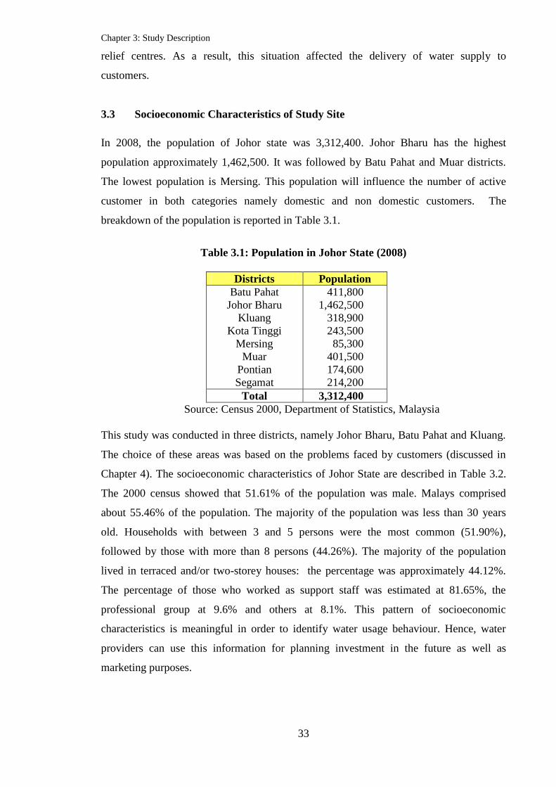
Chapter 3: Study Description
33
relief centres. As a result, this situation affected the delivery of water supply to
customers.
3.3 Socioeconomic Characteristics of Study Site
In 2008, the population of Johor state was 3,312,400. Johor Bharu has the highest
population approximately 1,462,500. It was followed by Batu Pahat and Muar districts.
The lowest population is Mersing. This population will influence the number of active
customer in both categories namely domestic and non domestic customers. The
breakdown of the population is reported in Table 3.1.
Table 3.1: Population in Johor State (2008)
Districts Population
Batu Pahat
Johor Bharu
Kluang
Kota Tinggi
Mersing
Muar
Pontian
Segamat
411,800
1,462,500
318,900
243,500
85,300
401,500
174,600
214,200
Total 3,312,400
Source: Census 2000, Department of Statistics, Malaysia
This study was conducted in three districts, namely Johor Bharu, Batu Pahat and Kluang.
The choice of these areas was based on the problems faced by customers (discussed in
Chapter 4). The socioeconomic characteristics of Johor State are described in Table 3.2.
The 2000 census showed that 51.61% of the population was male. Malays comprised
about 55.46% of the population. The majority of the population was less than 30 years
old. Households with between 3 and 5 persons were the most common (51.90%),
followed by those with more than 8 persons (44.26%). The majority of the population
lived in terraced and/or two-storey houses: the percentage was approximately 44.12%.
The percentage of those who worked as support staff was estimated at 81.65%, the
professional group at 9.6% and others at 8.1%. This pattern of socioeconomic
characteristics is meaningful in order to identify water usage behaviour. Hence, water
providers can use this information for planning investment in the future as well as
marketing purposes.
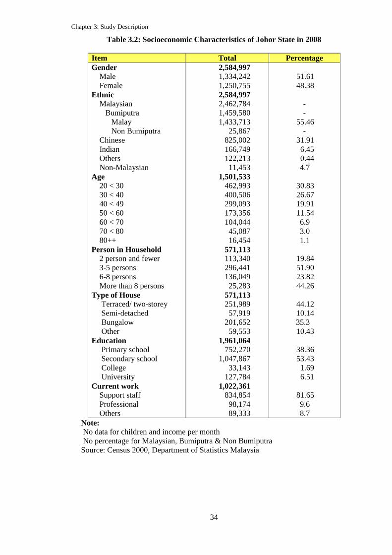
Chapter 3: Study Description
34
Table 3.2: Socioeconomic Characteristics of Johor State in 2008
Item Total Percentage
Gender
Male
Female
Ethnic
Malaysian
Bumiputra
Malay
Non Bumiputra
Chinese
Indian
Others
Non-Malaysian
Age
20 < 30
30 < 40
40 < 49
50 < 60
60 < 70
70 < 80
80++
Person in Household
2 person and fewer
3-5 persons
6-8 persons
More than 8 persons
Type of House
Terraced/ two-storey
Semi-detached
Bungalow
Other
Education
Primary school
Secondary school
College
University
Current work
Support staff
Professional
Others
2,584,997
1,334,242
1,250,755
2,584,997
2,462,784
1,459,580
1,433,713
25,867
825,002
166,749
122,213
11,453
1,501,533
462,993
400,506
299,093
173,356
104,044
45,087
16,454
571,113
113,340
296,441
136,049
25,283
571,113
251,989
57,919
201,652
59,553
1,961,064
752,270
1,047,867
33,143
127,784
1,022,361
834,854
98,174
89,333
51.61
48.38
-
-
55.46
-
31.91
6.45
0.44
4.7
30.83
26.67
19.91
11.54
6.9
3.0
1.1
19.84
51.90
23.82
44.26
44.12
10.14
35.3
10.43
38.36
53.43
1.69
6.51
81.65
9.6
8.7
Note:
No data for children and income per month
No percentage for Malaysian, Bumiputra & Non Bumiputra
Source: Census 2000, Department of Statistics Malaysia

Chapter 3: Study Description
35
3.4 Transformation of Johor Water Supply
SAJ Holdings (SAJH) is a subsidiary of Ranhill Utilities Berhad, which is Malaysia‟s first
“source to tap” water solution provider, offering holistic water services from engineering
and construction to treatment, distribution and services. It provides a fully integrated
service, i.e. it is involved in the all the processes of drinking water supply; these range
from raw water acquisition, treatment and purification, and the subsequent distribution of
purified water to customers, plus billing and payment collection.
SAJH was granted a concession for 30 years‟ potable water supply in Johor state, from 1
March 2000 until 2029 (Figure 3.1).
Source: SAJH (2006)
The Water Supply Department of Johor was originally formed in 1989 under the Public
Works Department. In February 1994, it became a corporate company, Syarikat Air Johor
Sdn. Bhd. In March 2000, it was transformed into a fully privatised company known as
SAJ Holdings Sdn. Bhd. (SAJH). This sequence of events is as shown in Figure 3.2.
Then, Runhill Utilities Berhad (RUB) was listed as a public listed company in June 2002.
Figure 3.1: SAJH Operational Area

Chapter 3: Study Description
36
Source: SAJH (2008)
Specifically, SAJH has put in place an operation and maintenance model, the purpose of
which is to plan and deliver enhancements to water service operations, manage and
improve the water distribution system and also maintain assets and optimise company
operations. This is in order to achieve the lowest possible costs through an effective
maintenance programme. In addition, effective management systems to regulate the
quantity and quality of water have been established.
There is also an initiative to create strategies to deal with various aspects of measurement
data and operating records, and also to carry out the management and development of the
entire programme of works. This includes items such as quality management, programme
and cost control, asset management and planning, procedure and contract strategies, and
monitoring construction (SAJH, 2008).
3.5 Water Treatment Process
There are two steps to the water treatment process as follows:
(a) Water Treatment
Water treatment is a process of removing impurities from untreated water, in order to
supply water which is good enough for human consumption. Among substances removed
are bacteria, algae, iron, sulphur and other chemical pollutants. The conventional
treatment plant comprises the following processes:
Figure 3.2: Transformation of Johor Water Supply

Chapter 3: Study Description
37
Source: SAJH (2008)
(i) Screening
Physical material such as wood, leaves, silt and others are screened at intake.
(ii) Aeration
Water pumped from the intake is oxidised for removal of taste and odour.
(iii) Coagulation / Flocculation
The chemical alum is added to allow small particles in the water to combine and
become bigger. They grow in size by knocking against each other. These particles
are called flocs.
(iv) Sedimentation
In sedimentation, heavy flocs are allowed to settle. Clarified water is then
collected from the top of the tank. If, however, the flocs are lighter, bubbles are
introduced. The flocs then stick to the bubbles and remain at the top of the tank.
Clarified water is then collected from the bottom. This process is called Dissolved
Air Flotation.
(v) Filtration
Filters are then used to trap fine particles in the water. The clean water then goes
to the clear water tank.
Diagram 3.1: Water Treatment Process

Chapter 3: Study Description
38
(vi) Disinfection/pH Adjustment
In the clear water tank, the water is disinfected to get rid of dangerous microbes.
The pH is also adjusted using lime or soda ash. Acidic water could cause
corrosion in pipelines.
(vii) Clear Water Tank
Water will be kept in the clear water tank before distribution. Here, water samples
are collected every two hours for testing to ensure that they meet with WHO
standards and that the water is safe for usage. The water treatment plant would
stop its operations if pollutants were discovered in any of the tests conducted. This
is, however, very rare, and most of the treatment plants in operation have never
experienced this.
Source: SAJH (2008)
(b) Water Supply Distribution
After the process, water from the water treatment plant is distributed to consumers, using
huge diameter pipe mains. Water is distributed by gravity, or pumped to the tank and then
distributed by gravity to customers.
Diagram 3.2: Water Supply Distribution

Chapter 3: Study Description
39
3.6 Water Infrastructure
3.6.1 Water Demand
In 2008, SAJH had 888,756 registered customers, consisting of 777,338 domestic and
111,418 non-domestic customers. This number was an increase of 3.04% compared with
active customers in 2007. There is also an uptrend of customers for each district. In 2007
and 2008, the majority of the customers were from Johor Bharu district. This was
followed by Batu Pahat and Muar districts. Water demand has a positive correlation with
the population. The breakdown of customers was as follows:
Table 3.3: Consumers by Districts and Categories in 2007 and 2008
District 2007 2008
Domestic Non-
Domestic
Total Domestic Non-
Domestic
Total
Johor Bharu 358,534 52,667 411,201 370,376 56,766 427,142
Kota Tinggi 44,097 4,768 48,865 44,550 4,957 49,507
Pontian 37,131 4,949 42,080 38,083 5,163 43,246
Batu Pahat 95,713 13,794 109,507 97,959 14,478 112,437
Segamat 51,477 6,302 57,779 52,582 6,653 59,235
Kluang 66,022 9,165 75,187 67,286 9,508 76,794
Muar 88,008 11,468 99,476 90,445 11,890 102,335
Mersing 15,740 1,863 17,603 16,057 2,003 18,060
Johor 756,722 104,976 861,698 777,338 111,418 888,756
Source: SAJH (2008)
3.6.2 Pipelines and Reservoirs
Pipelines are the most important aspect of the water infrastructure because water needs to
pass through them before reaching the customer‟s tap. The water quality is affected by the
material and age of the pipelines. There are many types of pipe. Pipes can consist of
asbestos cement, mild steel, ductile iron, cast iron, polyethelene, and uPVC. In total, the
length of distribution pipelines in 2007 and 2008 respectively was approximately
16,971km and 17,802 km, as shown below:

Chapter 3: Study Description
40
Table 3.4: Types of Pipe and Total Length (km)
Material Length of Pipes (km)
2007
Length of Pipes (km)
2008
Asbestos Cement 7,808 8,074
Mild Steel 2,918 3,067
Ductile Iron 1,273 1,314
Cast Iron 154 156
Polyethelene 607 630
uPVC 4,097 4,480
Other 113 80
Total 16,971 17,802
Source: Malaysia Water Industry Guide (2009)
Furthermore, there are 535 reservoirs in Johor, with a total capacity of 1,818.54 million
litres (Ml). Essentially, the number of reservoirs required is dependent on population
numbers, because each reservoir has a limited capacity of water that may be supplied to
residential customers. Reservoirs‟ main purposes include the following: providing a store
of treated water in order to minimise any stoppages caused by malfunctions of pumps,
mains, or any other equipment; acting as a release valve for a system which is kept
supplied via pumps; and sustaining a uniform water pressure across the system (Vipin
Bhardwaj et al., 2001). The breakdown of reservoirs by district is reported in Table 3.5.
Table 3.5: Number of Reservoirs in 2008
District No. of Reservoirs Total Capacity (Ml)
Johor Bharu 235 1,052.81
Kota Tinggi 53 107.01
Batu Pahat 48 197.34
Pontian 26 70.86
Kluang 59 153.32
Muar 48 120.31
Segamat 49 86.53
Mersing 17 30.36
Johor 535 1,818.54
Source: SAJH (2009)

Chapter 3: Study Description
41
3.7 Water Tariffs, Revenue and Expenditure
Johor has the highest average water tariff among states in Malaysia: approximately
RM0.98 per m3 for residential customers. This price has influenced by the cost of water
treatment. Moreover, changes in the price must be approved by SPAN. The price per m3
increases with domestic consumption based on the rate consumed in order to encourage
customers to use water wisely for water sustainability reasons, as it is a scarce resource.
The breakdown of the price per m3
is reported in Table 3.6.
Usage Category Rate (m³) Price Per m³
(RM)
Minimum Payment
(RM)
Domestic 015 0.38 4.00
1630 1.31
3145 1.82
46100 2.20
>100 2.23
Source: SAJH (2008)
Additionally, the water tariff will determine the revenue of the water company as well as
the percentage of payment of water bills. The company will achieve a profit if the revenue
exceeds the expenditure. Expenditure can be divided into two categories, namely capital
expenditure (OPEX) and operation expenditure (CAPEX). The expenditure and revenue
have shown a year-on-year increase until 2008, as shown in Table 3.7. In 2006, the
percentage for revenue over expenditure was approximately 61.2%, which was the
highest as compared with previous years, as well as with 2007 and 2008. These
fluctuations might be due to the increase of the cost of water treatment and maintenance
which occurred during those years.
Table 3.6: Water Tariff

Chapter 3: Study Description
42
Table 3.7: Expenditure and Revenue (MYR)
Year Expenditure Revenue +/-
2002 270,722,202 293,531,212 8.4%
2003 382,373,342 428,919,218 12.2%
2004 390,658,719 497,620,817 27.4%
2005 460,719,155 610,068,473 32.4%
2006 440,038,670 709,357,518 61.2%
2007 288,146,000 716,403,000 59.78%
2008 336,114,000 733,073,000 54.15%
Total 2,568,772,088 3,988,973,238
Source: Malaysia Water Industry Guide (2009)
3.8 Water Management, Planning and Monitoring
The aim of SAJH is to achieve efficiency and effectiveness in delivering a service to
customers. Therefore, SAJH developed measurable targets as below:
3.8.1 Setting of Measurable Targets
This target involves the quality objective and customer charter. The quality objective
includes the water quality (meeting the Ministry of Health Standards), continuous supply,
good water pressure, a safe working environment, environmental compliance, water
supply approval, the billing cycle, and Non-Revenue Water (Table 3.8). The customer
charter comprises water quality, pipe burst repairs, billing, pipe leakage, interruption, and
water supply connection (Table 3.9).

Chapter 3: Study Description
43
Customer Quality Quality Targets Achievement
2007
Water Quality (MOH
Standard)
99% compliance 99.5%
Continuous Supply No more than one scheduled
disruption of 24 hours per
customer per 90 days
100%
Adequate Pressure ≥ 10 metres residual pressure at
any point in reticulation
99.4%
Water Quantity (i) Min.120% supply capacity
against demand
(i) 100%
(ii) Min.12 hours storage
capacity at reservoir
(ii) 100%
Safe Working Environment (i) Zero penalties (i) 0 cases
(ii) Zero hospitalisations (ii) 8 cases
(iii) 100% PPEs compliance (iii) 28 cases
(iv) 1/1000 person/year time
lost through injury
(iv) 100%
Environmental Compliance Provide sludge treatment for all
plants if required
Effluent
discharge
continuously
monitored for
compliance
Water Supply Approval/CF
Support
(i) New connection for
developer 7 days
(i) 99.79%
(ii) Water supply approval 14
days after contribution
payment
(ii) 78.22%
(iii) 30 days CF support (iii) 91.76%
Billing cycle Average of 30 days 30.65 days
Non-Revenue Water NRW target set at 28% in June
2008 (concession target 20% by
2010)
31.5% as at
June 2007
Source: SAJH (2008)
Table 3.8: Quality Objectives
Chapter 3: Study Description
44
Criteria Target Achievement
Water shall be supplied in compliance with MOH
Standards:
(i) Residual chlorine; < 2.8% 2.76%
(ii) Aluminium; < 10.2% 4.59%
(iii) E. Coli; < 0.4% 0.0%
(iv) Turbidity; < 0.2% 0.08%
(v) E. Coli & residual chlorine. < 0.3% 0.0%
Customers shall be informed of all planned
interruptions more than 24 hours in advance.
100% 94.23%
Pipe bursts shall be repaired within 18 hours of receipt
of complaint.
100% 99.35%
Pipe leaks shall be repaired within 2 working days of
receipt of complaint.
100% 99.42%
Bill queries at the counter shall be attended to within ½
hour.
100% 99.91%
Queries & complaints requiring a visit to the premises
shall be attended as follows:
(i) Visit to the premises within 3 days of receipt
of complaint;
100% 94.00%
(ii) Complaint resolved within 10 days of receipt
of complaint.
100% 97.96%
New water meters shall be installed at premises as
follows:
(i) 2 working days after deposit paid for
individual household;
100% 98.98%
(ii) 7 working days after deposit paid for housing
developer.
100% 99.75%
Disconnected water supply shall be reconnected within
3 working days after the related payment is received.
100% 99.57%
Deposits shall be returned within 3 weeks of receipt of
application to terminate supply together with related
documents.
100% 80.65%
Application for approval of reticulation plans and
internal plumbing shall be responded to within 3
weeks of receipt of application.
100% 95.45%
Source: SAJH (2008)
Table 3.9: Customer Charter

Chapter 3: Study Description
45
3.9 Appraisal of SAJH
In order to achieve the goal and fulfil customers‟ expectations, SAJH has conducted
customers‟ perception studies every year. These studies used personal interviews carried
by well-trained research assistants. The findings of the customer perception surveys can
be reported based on two aspects for 2007 and 2008 as follows:
3.9.1 Service Quality
In 2007, the majority of respondents (estimated at 93%) did not know the quality of the
water they received. Approximately 79.6% of respondents were satisfied with water
quality and 13% were dissatisfied. Meanwhile, findings in 2008 showed that the majority
of the respondents were satisfied that the water supplied complied with Ministry of
Health requirements. However, half of the respondents did not know the standard water
quality they received. Approximately 91% of respondents were satisfied overall with
water quality. In terms of current colour, odour, and taste, only 75% of them were
satisfied and 22% were dissatisfied. All the respondents agreed the importance of having
better quality tap water which was safe to drink, clear and odourless.
Furthermore, the percentages of respondents who received advance notification for
planned water disruptions were 76.2% in 2007 and 68% in 2008, respectively. The most
effective channel of communication was through flyers. In 2007, about 93% of
respondents experienced interruptions to the water supply over the previous 6 months.
The main causes were pipe bursts and leakage at 27.90%, water rationing, estimated at
26.90%, and maintenance work, at about 28.40%. In 2008, half of the respondents have
experienced water supply interruption in the previous 6 months because of leakage and
pipe burst (42%) and maintenance by contractors/SAJH (estimated at 43%).
Approximately 91% of respondents were also satisfied with the water pressure.
There were slight differences in the level of customer concern in 2007 compared with
2008. For the year 2007, where having tap water that is safe to drink, clear and odourless
was the highest priority for approximately 66% of respondents; having a water supply
which was adequate, with no interruptions except in emergencies was the priority for
33%; while only 0.2% of respondents were concerned with having information about
SAJH and service provided. However, in 2008, the percentage of customers concerned
that tap water is safe to drink, clear and odourless was 79.26%; those who required

Chapter 3: Study Description
46
information about SAJH and services provided were estimated at 67.04%; those whose
priority concern was that the water supply was adequate, with excellent customer service
were about 59.52%; and those who wished never to have any interruption in service
except during emergency cases were 56.55%.
In 2007, 87% of customers believed that the current status of the water supply
infrastructure was in good condition and there was a need to invest for minimum
improvement; approximately 12.4% thought it was in bad condition in a few aspects and
needed to improve in those aspects; and 0.3% thought it was in very bad condition and
needed to improve. 86.2% were also satisfied with the services provided. Their feelings
with regard to the standard services of SAJH were that 47% thought they needed
improvement, and 53% thought services should remain as they were. The majority of
respondents (51.8%) were not willing to pay more for the water services provided;
approximately 43.3% agreed with paying more.
However, in 2008, 75% of customers agreed that the overall service provided was
excellent, and those „satisfied‟ were about 20%. Their feelings on the standard of service
can be classified as follows: an estimated 52% were in favour of making improvements to
the level of service, and about 43% wished the current standard of service to remain. As
far as willingness to pay in order to improve the level of service was concerned, 64% of
respondents disagreed and only 18% agreed.
In conclusion, the majority of respondents were not willing to pay for improvements to
the level of the water supply service. Surprisingly, the percentage of respondents who
preferred to improve the level of service rather than maintain the current standard
increased from 47% in 2007 to 52% in 2008. This situation might arise because they
assume that water is a basic need, therefore, the water tariff should not be raised. At the
same time, the cost of living continuously increased.
3.9.2 Customer Charter
The main objective of an organisation‟s Customer Charter is to increase customer access
to services and encourage the quality of those services. It does so by informing the
customers of the standards of service which they should expect, how to contact the
organisation, and what they should do if they are dissatisfied with the service provided.
From the employees‟ point of view, such a charter is a benefit, as it ensures that the

Chapter 3: Study Description
47
services offered by the organisation are clearly laid out (Paternoste, 2010). The SAJH
customer charter comparison study for 2007 against 2008 is reported in Table 3.10.
Very
Satisfied
Satisfied Dissatisfied Year
Complaints will be
settled within 10 days
from date of receipt of
complaint.
- 48.5% 38.8% 2007
28% 65% 5% 2008
Disconnected water
supplies will be
reconnected within 2
working days of
receiving payment of
arrears.
- 62% 24% 2007
30% 58% 4% 2008
Water meters for
individual households
will be installed
within 2 working days
of receiving deposit.
- 85% 8.9% 2007
41% 52% 5% 2008
A visit by a customer
to the water
company‟s premises
will be responded to
within 3 working days
from date of receipt of
complaint.
- 69.7% 24% 2007
34% 61% 3% 2008
Leakages will be
repaired within 2-3
days of notification
within working hours.
- 65.5% 28% 2007
33% 60% 5% 2008
Burst pipes will be
repaired within 18
hours of notification.
- 77% 12.5% 2007
31% 61% 6% 2008
Note: No data for very satisfied in 2007
Source: Customer Perception Survey in 2007 and 2008
There were dramatic changes of customers‟ perception of all aspects of the customer
charter between 2007 and 2008. The highest percentage of „very satisfied‟ or „satisfied‟
customers in 2008 was an estimated 95% for a response within three working days of a
visit by the customer to the company‟s premises. This was followed by complaints being
Table 3.10: Customers’ Perception on Customer Charter for 2007 and 2008

Chapter 3: Study Description
48
settled within 10 days (approximately 48.5% and 93% in 2007 and 2008, respectively).
Similar results occurred for the installation of water meters and leakages repaired within
2-3 days of notification (approximately 93% in 2008). Surprisingly, there was an increase
in customer satisfaction concerning the repair of burst pipes within 18 hours from 77% to
92% between the 2007 and 2008 surveys. In addition, 12.5% of customers were very
dissatisfied about the repair of burst pipes in 2007. These situations showed the
improvement of the water service provided by SAJH. Nowadays, customers are more
concerned about the level of service provided by the water operator (Goett et al, 2000),
particularly water quality, which has a direct impact on health problems.
In summary, the feedback from these surveys is important to SAJH in setting a
benchmark and the need for continuous improvement and further development to meet
customers‟ perceptions and satisfaction. For instance, SAJH should educate the public on
the priority of investing in the water supply.
3.10 Non-Revenue Water (NRW)
According to Asian Development Bank (2010), non-revenue water (NRW) can be defined
as the difference in volume between the amount of water leaving the treatment plants and
that for which customers are billed. There are three components of NRW as follows:
(a) Physical (i.e. real) loss of water consists of leaks throughout the system and
reservoirs overflowing. This is caused by failure to actively control leakage, the
poor quality of assets underground, and poor operations and maintenance
procedures.
(b) Commercial (i.e. apparent) loss of water is caused by consumption being under-
recorded by faulty meters, errors in data handling, and water being stolen by
various means.
(c) Also, certain authorised consumption of water is unbilled. This includes that used
by firefighters, that used by the company itself in its operations, and that made
available free to particular consumer groups.
At the moment, NRW is estimated at 24.9%, which is reduced from 30%. NRW is the
crucial factor influencing water revenue. As previously mentioned, SAJH has invested
more capital for delivery of safe, high quality water to customers. Therefore, SAJH has to
reduce NRW to ensure that revenue exceeds capital and operating expenditure. In 2004,

Chapter 3: Study Description
49
SAJH implemented the NRW Strategy and Action Plan, which focused on improvements
in addressing, managing and monitoring various NRW issues. The response strategy
includes the following:
(a) Awareness: elements causing NRW are bursts, leaks, reservoirs and meter
malfunctions. These can be encountered at any time, and will influence NRW
levels. If reservoir levels, system flows and pressure are monitored at significant
points, this will result in quicker action to resolve problems.
(b) Location: NRW levels will also be affected by the time taken to discover the exact
reasons for loss. For instance, a loss caused by a reservoir overflowing can be easy
to determine, whilst others such as a small buried leakage need a longer time to
investigate.
(c) Repair: when the exact cause of the loss has been identified, repairs will be
carried out with better quality materials in order to avoid repetition of the
problem.
Other initiative tools also used include the Job Management System (JMS), Remote
Monitoring System Installation, District Metering Zones Establishment, Customer Meter
Management, and Production Meter Management.
3.11 Water Quality
According to National Water Quality Handbook (2003) a working definition of water
quality is its biological, chemical, and physical makeup in relation to the uses for which it
is intended (such as drinking, irrigation, fishing and recreation).
Water quality is the most important attribute to be considered when attempting to
improve the water supply service. Therefore, SAJH water quality should comply with the
Ministry of Health‟s Drinking Water Quality Guidelines (MOH Guidelines) in physical,
chemical and microbiology aspects. Currently, 29,036 water samples have been tested
and 234,928 tests have been carried out on these.

Chapter 3: Study Description
50
The strategic plan was put into practice to ensure that the MOH Guidelines were
complied with. The guidelines include levels of pipework scouring and reservoir cleaning
procedures, in order to enhance consumer water quality (Summerill, 2010). Within the
network system, there are five secondary chlorine closing systems installed.
Sampling activities were affected because the plants were shut down due to the floods of
December 2006 to January 2007. In order to solve this issue, SAJH increased water
quality monitoring, consisting of treatment plants, tankers and static tanks. SAJH
developed the Central Laboratory located in Sri Gading, Batu Pahat to test water samples
of water for compliance with the MOH Standards (SAJH, 2008).
The objectives of the Central Laboratory are:
(i) to co-ordinate the associate district laboratories and suppliers as well as
private laboratories where samples of water from each plant are sent;
(ii) to troubleshoot, should the district laboratory assistant be unable to
diagnose or manage a water quality problem;
(iii) to arrange training of operators and laboratory assistants;
(iv) to communicate with MOH officers concerning any water quality
violations;
(v) to contribute to the monitoring of trends in water quality;
(vi) to maintain a database of historic results;
(vii) to purchase glassware and reagents for use in the plant laboratory.
Whereas the roles of the District Laboratories are:
(i) to monitor the water quality in the district plant and troubleshoot any
problems;
(ii) to carry out water quality spot checks in the plants;
(iii) to monitor and control measurements to ensure water quality and record-
keeping targets are met;
(iv) to calibrate and check the accuracy of instruments in a planned manner, to
ensure instrumentation is fully functional;
(v) to deal with the plant concerning the laboratory‟s glassware and chemical
reagents requirements.

Chapter 3: Study Description
51
At the moment, there are 975 sampling points throughout the water supply system. New
sampling points will be installed in order to fulfil the increasing number of connections
(Eighth Malaysia Plan, 2001). The Water Quality Information System (WaQIS) software
system is employed to consolidate the water quality test results and interpret the water
quality performance for the entire state of Johor.
In addition, the Central Laboratory utilises the latest technology instruments, such as the
Atomic Adsorption Spectrometer (AAS) and Gas ChromatographyMass
Spectrophotometer (GCMS), to identify heavy metals, trihalomethane (THM), and other
pesticide content in raw and treated water, as well as other organic pollutants for short
periods. Then, the formulation of the strategic Water Quality Action plan includes
preventative measures and remedial action procedures that consist of reservoir cleaning
and an air-scouring programme, to upgrade water quality.
SAJH has also hired 40 reliable and well-trained staff for the Water Quality Department
to perform analysis and sample and test the physical, chemical and microbiological
characteristics of more than 35,000 water samples per year, on which 300,000 water tests
per year are conducted.
Approximately 99.5% of the water quality samples tested passed the required standard as
outlined in the MOH Standards. In September 2005, SAJH‟s Central Laboratory was
awarded ISO/IEC:17025 certification by the Department of Standards of Malaysia
(SIRIM). SAJH also introduced water tank cleaning: the first scheduled tank cleaning
programme in Malaysia.
3.12 Network
In 2000, SAJH developed a customer call centre, which operates 24 hours, 7 days a week.
This is the first such technology adopted in the Malaysian water industry. It serves as a
nerve centre to receive feedback and complaints from customers. The Job Management
System (JMS) is a database to receive customer feedback, turning it into job assignments
and job status reports. This information is meaningful for evaluation, planning, decision-
making, and management action. Currently, the SAJ Info Centre receives an average of
2275 calls per week about a variety of issues, for example damage enquiries, meter
problems, water quality, billing enquiries, water theft, leakages, lack of water supply,

Chapter 3: Study Description
52
tanker requests, pipe bursts, and poor water pressure. The number of calls has increased
by 8.8% since 2006. This shows that customers are more concerned about water wastage
and have taken action to conserve water.
In 2006, there was an average of 666 pipe bursts per month. This decreased to an average
of 615 cases per month in 2007. This was due to the Asset Replacement Department and
Pressure Management Programme completing the replacement of pipes. Pressure-
reducing valves (PRVs) were inserted into the network at certain critical positions under
the Pressure Management Programme, in order to lower the number of occurrences of
burst pipes. At present, approximately 98.1% of burst pipes are repaired within 18 hours.
Furthermore, due to improved detection of leaks and better customer feedback, 1850
repairs of minor leaks per week have been achieved: an increase of approximately 25%
from 2008. The performance standard for the time to repair pipe leaks was decreased in
September 2006 from three to two days. It is estimated that about 95% of minor leakages
have been repaired within two days since then.
The Network Department and the NRW Department collaborate closely together in order
to achieve the NRW target levels by managing the implementation of the NRW Strategy
and Action Plan. The Network Department was responsible for monitoring and
controlling the water crisis in Segamat, Muar, Johor Bahru and Kota Tinggi during the
major floods which affected Johor state of Johor in December 2006 and January 2007
(SAJH, 2008).
3.13 Asset Replacement
In the Second Operating Period programme (from 30 June 2007), 668 km of asbestos
cement pipes were replaced by the Asset Replacement Department. Also, under the
Rehab programme in 2006 and 2007, 77 km of asbestos cement pipes were replaced.
Major pipe repair and replacement work took place following the two floods in December
2006 and January 2007. In total, MYR9.3 million was assigned for work to prevent
landslides and conduct repairs, and a further MYR4.4 million in order to replace damaged
pipes. Also, because of various upgrading and development works by the authorities,
some relocation of pipes by SAJH was required. In all, during the Second Operating

Chapter 3: Study Description
53
Period, MYR12.0 million was spent on such works requested by the authorities. Another
MYR1.8 million was spent for works requested since 2006 that marked the beginning of
the Third Operating Period (SAJH, 2008).
3.14 Conclusions
SAJ Holdings Sdn. Bhd. was fully privatised in March 2000. It functions as a structured
water system supply company dealing with the total cycle of the drinking water supply
system. The process starts sourcing of raw water, treatment and deliver of treated water to
consumers, issuing of bills and collection of payments.
Johor state was chosen as a case study. The survey was be conducted in three districts
included Johor Bharu, Kluang, and Batu Pahat. These areas were chosen to represent
problematic areas in Johor that experience issues such as water quality, pipe burst and
leakage, interruption, and water pressure. The main demographic characteristics of the
state are as follows: an estimated 55.46% of the population are Malay and 51.61% are
male (based on the 2000 census). Meanwhile, the majority of the population has a
primary and secondary school education (approximately 91.79%).
The number of customers continually increased approximately 3.04% between 2007 and
2008. Currently, SAJH have 888,756 registered customers. The water infrastructure,
including pipelines and reservoirs, was considered as the main attribute influencing the
water supply service. Additionally, water tariffs, revenue and expenditure are the most
important aspects to determine the viability of project investment.
Johor has the highest water tariff in Peninsular Malaysia: about RM0.98 per m3 for
residential customers. Basically, water tariffs increased when consumption rises, in order
to achieve water sustainability. The tariff is the primary determinant of SAJH‟s revenue,
rather than other income such as the connection and installation fees.
The appraisal of SAJH concentrated on the customer charter as the basis for the main
attributes of this research, such as leakages and burst pipes. The analysis referred to the
customer survey that is conducted every year to evaluate the level of service provided to
the residential customer in particular. The results demonstrated that the service level has

Chapter 3: Study Description
54
improved in certain aspects, while other aspects need to be improved. One of the critical
aspects is NRW, which is still high: this needs to be resolved by SAJH.
Other categories such as water quality, asset replacement and water network also
influence the overall service level. The integration of all aspects is very important to
achieve efficiency and effectiveness in delivering safe drinking water. Therefore, SAJH
should invest for the future.

Chapter 4: Methods and Procedures
55
CHAPTER 4: METHODS AND PROCEDURES
4.1 Introduction
This chapter describes the methodology applied in this research. It starts with the
properties of discrete choice models and the specification of Conditional Logit (CL) and
Mixed Logit (MXL) models. This study will employ a CE to measure customers‟ WTP to
improve water supply for residential customers in Malaysia, particularly in Johor state.
Then, the detailed stages of CE are also presented. It also mentions the process of
fieldwork data collection, including the pilot test, sampling design, and the justification of
selecting three districts in Johor state.
4.2 Properties of Discrete Choice Models
4.2.1 Choice Set
In discrete choice models, decision-makers include households, people and other units of
decision-making. They choose amongst alternatives such as water attributes, product
attributes and so on. The set of options within the choice set must accomplish three
features. First, the options must be mutually exclusive: this means that selecting one
option equals not being allowed to choose any of the others. The person making the
decision has to select one option only from the set of choices. Second, this set has to be
exhaustive, i.e. it must comprise all possible options. The decision-maker is asked to
choose one of the options. Third, the number of options must be limited (i.e. not infinite).
The alternatives may be listed and one eventually reaches the end of the list (Train, 2000).
This is what makes the distinction between discrete choice analysis and regression
analysis, which in theory allows for an infinite number of options.
To take an example, there can be a number of alternatives forming the choice set for a
person deciding how to get to work: driving on one‟s own, car sharing, using the bus or
train. However, the options may become more complicated because one could use
multiple modes of transport for a particular trip, e.g. driving one‟s car to a railway station
and taking the train from there. Therefore, the choice set can include every possible
combination of transport modes. As an alternative, the choice may be defined as that of
the “primary” mode: in this case the set comprises only bus, car, train and “other”

Chapter 4: Methods and Procedures
56
(encompassing all other possibilities such as walking or using a bicycle; “other” is used to
ensure the choice set is exhaustive).
4.2.2 Identification of Choice Models
The specification and estimation of the discrete choice model are affected by the
behavioural decision process. There are two parts as follows:
(a) Differences in Utility
The actual degree of utility is immaterial, both to the decision-maker‟s behaviour as well
as to the researcher‟s model. If one were to add a constant to the utility of all the possible
alternatives, the one with the highest utility would remain the same (Train, 2000).
The choice probability is )0(Prob)(Prob ijUUijUUP njninjnini , which
depends upon the differences in utility. However, if the utility consists of observed and
unobserved parts, the choice probability becomes )(obPr ijVVP njnininjni
which is based on the differences. This indicates that only variations in utility matter,
which has implications regarding the recognition and specification of discrete choice
models (Train, 2003). Basically, it will take several forms, as below:
(i) Alternative Specific Constants (ASC)
It is satisfactory to assign the observed part of the utility to represent a linear
parameter, including the constant (Train, 2000). The equation is written as:
jkxV jnjnj '
where:
njx = vector of variables that relate to alternative j as faced by decision-
maker n
= coefficient
jk = constant specific to alternative j
The alternative specific constants (ASC) have a similar role with the constant in
the regression model (Train, 2003) because they capture whatever orderly
variations in the choice observations which are related with an option that is

Chapter 4: Methods and Procedures
57
explained neither by the observed socioeconomic characteristics of the
respondents nor by the attribute variation (Othman et al., 2004).
When alternative specific constants are present, the unobserved portion of utility,
nj , then possesses zero mean by construction. However, since only the variations
in utility are relevant, so are only the variations in the alternative specific
constants, not their absolute values. To reflect this, the researcher must set their
overall level (Train, 2003).
(ii) Socioeconomic Variables
Entering socioeconomic variables will affect the model. Generally, the main
attributes vary among alternatives. However, the attributes of the decision-maker
do not vary amongst alternatives. For instance, the person‟s income will affect the
willingness to pay a price rise for every cubic metre of water if the water provider
improves the water service in terms of water quality or pressure. This result
indicates that a person‟s utility service depends on higher income. The
socioeconomic variables affect the differences in the utility service through their
interaction with the attributes of the alternatives.
(b) The Scale of Utility is Irrelevant
In the same way that adding a constant to all the alternatives‟ utility will not change the
choice of the decision-maker, neither will multiplying each alternative‟s utility by a
constant. The choice which possesses the highest utility remains the same, regardless how
utility is increased (or reduced). This means that it is not an issue how utility is scaled.
However, the standard process to normalise the scale of utility is by links between the
variance of the error terms (Train, 2003). As a result, normalising the variance of the error
terms is equivalent to normalising the scale of utility (Train, 2003).
4.2.3 Statistical Significant of Model Estimates
An outcome in statistics is considered to be „statistically significant‟ if the likelihood is
that it has not occurred by chance. Moreover, this is different from the use of the term
significance. Significance is a statistical term that states how certain we are that a
difference or relationship exists. The relationship of significance can be strong or weak.
Significant differences can be large or small.

Chapter 4: Methods and Procedures
58
The amount of evidence necessary to show that an event is not likely to have occurred by
chance is called the level of significance or critical p-value. The level of significance is
usually represented by the Greek symbol α (alpha). The most common levels are 5%
(0.05), 1% (0.01) and 0.1% (0.001). If a significance test produces a p-value lower than
the level of significance level, the null hypothesis is then discounted (Hill et al., 2007).
In order to analyse the panel data, this study will be an applied SAS program. The
procedure, which is called MDC (Model of Discrete Choice), will perform calculations on
a variety of multivariate random utility models, consisting of conditional logit, nested
logit, HEV (Heteroskedastic Extreme Value) and multinomial probit models. However,
this research will focus on only two models, multinomial logit (MNL) and mixed logit
(MXL).
Normally, the SAS results reveal information under the headings “Model Fit Summary”,
“Discrete Response Profile”, “Goodness of Fit Measures” and “Parameter Estimates”.
However, the statement algorithm converged at the beginning of the model. The most
important analysis is to evaluate whether to consider the estimated parameters in the
model as representing real effects. If the p-value of the parameter is high, it is considered
non-significant, since there is a high probability that a parameter estimate of the same size
can be generated, even when the true model parameter is zero; whilst if it is low, then it is
considered to be significant, and one can be more certain that the parameter estimate
represents a true effect. This is very practical data in assessing the parameters of the
model (Lívia Madureira et al., 2007). Those insignificant parameters can be ignored when
trying to judge whether the parameters that are significant correspond to the beliefs about
the relationship between the effects in the question and the behaviour (Markley, 2007).
4.2.4 Limitations of the MNL Model
(a) Taste Variation
Generally, the importance or value that decision-makers confer on each attribute of the
options differs among themselves (Train, 2003). For instance, water quality is probably
more important to households with a higher income level than those with a lower income.
Different respondents will choose different options depending on their individual
preferences and concerns, even they have the same education, income, job and so on.

Chapter 4: Methods and Procedures
59
As a result, MNL can represent systematic taste variation, but not random taste variation.
It can capture taste variations, but only in a very limited fashion. More precisely, tastes
that are consistent with reference to observed variables can be covered, but those that
vary with unobserved variables or strictly randomly cannot be handled (Train, 2003).
(b) Substitution Patterns
If representative utility is required by the research, MNL must utilise proportional
substitution throughout all the options. This means that altering the attributes of one
option, e.g. price, increases or decreases the probability of its being decided (Train,
2003). For example, when the water provider increases the water tariff for each cubic
metre, customers will decrease the quantity of daily usage and use water wisely. Instead
of using potable water, they will change to rainwater or well water.
Therefore, MNL employs a certain pattern of substitution across alternatives. MNL is also
appropriate, whenever replacement occurs in this way, given the researcher‟s
specification of representative utility (Train, 2003).
(c) Repeated Choice over Time
In research, there are numerous choices between various alternatives made by each
decision-maker. Typically, respondents are faced with a series of hypothetical choice
enquiries, called “stated preference” experiments. A set of alternative options with
different attributes will be presented to respondents (Train, 2003). Respondents are
required to decide how their choice will change when the attributes change (Yohei
Mitani, 2008). Consequently, the researcher indicates the sequence of choices by each
respondent. Data that represent restated choices like these are addressed in panel data
(Train, 2003).
MNL can be applied to examine the panel data, if the unobserved factors that impact
decision-makers are independent across the repeated options. However, dynamics- related
factors with unobserved factors cannot be managed, because the unobserved factors are
assumed to be unrelated over options (Train, 2003).

Chapter 4: Methods and Procedures
60
4.2.5 Panel Nature of Data
As mentioned above, in stated preference experiments, respondents are faced with a series
of hypothetical choice enquiries and are asked how their choices would alter when the
attributes do. Information collected in this way, that represents a series of different
choices by the same individual, is called panel data. In other words, panel data refers to a
set of data on the same individual over several periods of time (Maddala, 2001).
4.2.6 Taste Heterogeneity
The options chosen by the respondent constitute differences in utility, according to the
decision rules. In order to describe the type of heterogeneity in the population, direct
measures of taste are employed to capture the psychological factors affecting decisions.
For instance, the respondent will be faced with a series of options about their preferences
of attributes of non-market goods and ask them to determine their preferences between
the alternatives presented.
In addition, heterogeneity can be separated into observed and unobserved categories. In
terms of observed heterogeneity, the preference heterogeneity among individuals can for
instance be captured when using the interaction between attributes and individual-specific
variables (i.e., socioeconomics) (Pollack and Wales, 1992). In the random parameter
framework, by contrast, coefficients of attributes are broken down into a mean value that
presents the average attitude over the whole sample. Meanwhile, a deviation from the
mean is specific to each person in the sample. Based on this pattern, heterogeneity is
summarised applying a parametric density function for the coefficients in the model.
Hence, the proportion of the sample which prefers an attribute and that which does not
can be estimated (Train, 1998).
Mixed logit is extensively used in the random parameter discrete choice model that
represents preference heterogeneity in many fields, such as marketing (Louviere et al.,
2002; Ben-Akiva et al., 1999b) and non-market valuation (Train, 1998; Von Haefen et al.,
2004).

Chapter 4: Methods and Procedures
61
4.3 Theoretical Framework
The choice experiment1 method derives from random utility theory (Luce, 1959;
McFadden, 1974; Thurstone, 1927) and the characteristics theory of value (Lancaster,
1966). Random utility theory (RUT) is an example of a discrete choice econometric
model. It makes the assumption that the individual is perfectly able to make choices
which are fully informed; but also assumes that the researcher does not have all the
information and consequently must take uncertainty into consideration (Manski, 1977). In
choice experiment, individuals choose between different sets of (environmental) goods;
these are depicted in terms of their characteristics (or “attributes”) and attribute levels.
One of these attributes is usually price (Hanley et al., 1998); estimates of marginal utility
relating to changes in attribute level may be translated into monetary terms (Hanley et al.,
2002).
In order to identify the choice of the water supply attributes which is preferred by most
people, choice experiment (CE) has been employed. Essentially, the choice experiment
method consists of characteristics theory of value and random utility theory (Rolfe et al.,
2004).
Basically, RUT comprises two components, namely representative utility (observable)
and random components (unobservable). An individual will evaluate each alternative
from J.Uj;j ..,1 possible alternatives. The decision-maker must compare
UJUUU j ....,,..., 21 and choose the alternative with the maximum utility. In other words,
RUT assumes that the probability of decision-maker n choosing alternative j is the
difference between random components of alternatives j and i less than the difference
between the representative utilities of alternatives i and j for all alternatives in the
choice set (van Bueren et al., 2004; Ryan et al., 2009). Decision-maker n chooses
alternative i if and only if njni UU , ji (Train, 2003). Furthermore, the analyst will
observe the attributes of alternatives njx and socioeconomic characteristics of decision-
maker ns . Therefore, the utility function is denoted as )( , nnjnj sxVV and known as
representative utility (Train, 2003).
1 The choice experiment method has been referred to in the literature by a range of names, especially
more recently: “stated choice”, “attribute-based stated choice”, “choice-based conjoint”, and “choice
modelling”. This study uses the terms “choice modelling” and “choice experiment” interchangeably.

Chapter 4: Methods and Procedures
62
Normally, the equation of the utility is represented as njnjnj VU , where nj is the
random factor. The joint density of the random factors vector njnin ... is denoted
as )( nf . Then the probability of decision-maker n choosing alternative i can be
expressed as:
niP Prob )( njni UU
Prob )( njnjnini VV
Prob )( njnininj VV (4.1)
This probability is a cumulative distribution; the probability that each random term
njni .... is below the observed quantity njni VV . Then, using the density )( nf , this
equation can be rewritten as:
niP Prob )( njninj VVni
= ijdfVVI nnnjnininj ,)()(
(4.2)
where I (.) is the indicator function, which is 1 when the expression in the parentheses is
true, and 0 otherwise (Train, 2003).
It is complex to predict respondents‟ preferences because of the random component‟s
influence. This component allows the modelling of the choice of options in a probabilistic
form: the probability that individual n will choose option i from the choice set over the
other options j may be expressed as:
Prob )|( Ci Prob ,jnjninin VV all Cj (4.3)
where:
C = complete choice set
To estimate an equation (4.3), it is presumed that random elements are independent and
identically distributed (McFadden,1974) and Type 1 extreme value distribution or
Gumbel-distribution (Weibull). Then, the probability of choosing i can be given by:
Prob )(i = Cj
vj
vi
exp
exp (4.4)

Chapter 4: Methods and Procedures
63
where:
= scale parameter. This is inversely proportional to the standard
deviation of the error distribution, and is generally assumed have a
value of 1.
Equation (4.4) can be calculated by means of a multinomial logit or conditional logit
model (CL) that has to obey the IIA property. This means that the relative probabilities of
two choices are unaffected when they are either inserted into or taken away from the list
of alternatives (Ben-Akiva and Lerman, 1985).
Therefore, the probability of an individual‟s choice, where they are facing two
alternatives i or j, can be expressed as (Boxall et al., 1996):
Prob )(i Prob )( ijji VV
or
Prob )( j = Prob )( jiij VV (4.5)
Then, to estimate the linear-in-parameters utility function for the jth
alternative as follows
(Blamey et al., 1999):
)*(...
)*(... 11332211
jpp
jkkjj
ASCS
ASCSXXXXASCV
(4.6)
where:
= vector of coefficients
X = vector of observable characteristics of alternative i or j
p = socioeconomic characteristics
j = alternatives in the choice set
k = attributes or factors
= vector of utility values associated with vector of individual respondent
differences
Moreover, ASCs capture the unexplainable factors which can explain choice mean effect
in the error terms for each alternative (Ben-Akiva and Lerman, 1985). Socioeconomic
characteristics can be included in the model interactively with ASCs (Swallow et al.,

Chapter 4: Methods and Procedures
64
1994). ASCs also relieve inaccuracies caused by the assumption that IIA is violated
(Train, 1986).
When the parameter estimates have been obtained, the estimation of welfare can be
derived from WTP, according to Hanemann (1984); Parsons and Kealy (1992), Alvarez-
Farizo and Hanley (2002), Hurlimann and McKay (2007); and also the method used by
van der Pol and Ryan (1996), which can be derived as follows:
i
i
i
i
yV
V
InbWTP0
1
1
exp(
exp(
(4.7)
Equation (4.7) can be simplified as follows:
y
c
b
bWTP
where:
cb = coefficient of any of the attributes in the model
yb = coefficient on price
However, if the IIA is not violated, the standard random utility model can no longer
water quality (Train, 1998); consumers‟ choices of efficiency level of household
appliances (Revelt and Train, 1998); be employed. There are more complex statistical
models, including the random parameters logit (Train, 1998), the nested logit (McFadden,
1981) and also the multinomial probit (Hausman and Wise, 1978). IIA may be tested via
Hausman and McFadden‟s method (1984).
4.4 The Mixed Logit Model (MXL)
Mixed logit2 models have been applied to numerous examples of environmental analysis,
e.g. householders‟ WTP for various attributes of water services (Hensher et al., 2005);
WTP for an upgrade to fish stock, affected by anglers‟ choices of fishing sites and the
individuals‟ choices of vehicle based on emissions and fuel consumption (Train and
2 Mixed logit is also known as logit kernel probit or logit kernel, and random parameter logit or random
coefficient logit. This research prefers to use mixed logit due to it composed of mixture of logit models.

Chapter 4: Methods and Procedures
65
Sonnier, 2004) and demand for generation of renewable energy, for instance water and
wind power (Goett et al., 2000);
There are advantages of mixed logit specification, as follows: the model may be obtained
via utility-maximisation, and the IIA property is not revealed; it explains possible
correlations between recurring selections by each respondent. The model is also able to
portray circumstances in which the coefficients have a distribution pattern different from
the normal distribution (Brownstone and Train, 1996; Revelt and Train 1996).
Consequently, if a normal distribution is imposed in such cases, it is possible to obtain
results which may be improbable or counter-intuitive when utilising the estimates from
the model.
The specification adopts the mixed logit developed by Revelt and Train (1998) and Train
(1997). Individual n faces a choice among J alternatives in each of T time periods. J
can be as small as 2, and T can be small as 1. Hence, the person‟s utility from alternative
j in the period t can be written as follows:
njtnjtnnjt XU ' (4.8)
where:
njt is assumed to be an extreme value of IID independent of n
Individual n chooses alternative i in period t if iU jnjt . Moreover, the coefficient
vector n is unexplained, for each n diversifies among the population with density
)|( f where represents the parameters of this distribution. If n is specified to be
the same for all respondents, then is its value for all respondents; however, if n is
specified to be normally distributed in the population, represents the mean b and
covariance W .
Normally, the respondent chooses the situations that provide the maximum utility.
Therefore, the person‟s chosen alternative in period t is denoted as nty , the person‟s
sequence of choices over T time periods as Tyyy nnn ,...,1
, and the set of nny as Y .
The probability is conditional on n , then respondent i choosing alternative j in
situation t is standard logit (McFadden, 1974):

Chapter 4: Methods and Procedures
66
j
X
X
nnnjtn
nitn
e
etiL
'
'
)|,(
(4.9)
where ntie is independent over choice experiments. The conditional probability of the
respondent‟s n sequence of choices the product of the logit is:
)|()....|1,()|( ,1 nnTnnnn TyLyLyP (4.10)
If the researcher does not observe n , these conditional probabilities are integrated over
all possible values of n , using the density of n :
dfyPyP nn )|()|()|( (4.11)
where )|( nyP is the probability of the sequences of choices by the respondent,
conditional on the parameters of the distribution ).|( f According to McFadden and
Train (2000), any choice model may be closely approximated in an arbitrary manner by a
mixed logit which has a suitable specification of ).|( f
Generally, the integration of mixed logit probability has no closed form. Therefore, it has
to be approximated numerically via simulation. Practically, R draws of are taken from
density ).|( f The product in Equation (4.10) is calculated for each draw. The results
are then averaged over all draws. Then, the simulated probability, denoted )|(~
nyP for
this average, is:
)|(1
)|(~
r
r
nn yPR
yP (4.12)
The population parameter is calculated by introducing )|(~
nyP for each individual
into the log-likelihood function and function over . The estimator is consistent if R is
considered to increase with the size of the sample, and is asymptotically equivalent to the
estimator of the maximum likelihood on the (infeasible) exact probabilities, and
asymptotically normal and efficient if R increases faster than the square root of the size of
the sample (Lee, 1995; Hajivassiliou and Ruud, 1994). Halton draws are utilised to carry
out the simulation, as the results will be more accurate when estimating mixed logits than
random independent draws (Bhat, 2001; Train, 2000; Hensher, 2001a).

Chapter 4: Methods and Procedures
67
4.5 Design Stages in the Choice Experiment
In order to construct the CE questionnaire, there are five steps (Louviere et al., 2000,
Rolfe et al., 2004). These are: the definition of attributes, the assigning of attribute levels,
the creation of scenarios, the determination of choice sets and acquisition of preference
data, and the estimation of model parameters. Similarly, studies by Bateman et al. (2002),
and Mohd Rusli Yacob and Ahmad Shuib (2009) suggested that CE has five stages,
including the selection of attributes, the determination of levels, the choice of
experimental design, choice sets construction, and the of measuring preferences.
However, the experimental design and constructing the questionnaire were identified as
the most important stages in CE.
4.5.1 Defining Attributes
Definition of attributes is the most crucial stage in CE. Environmental goods or services
can be characterised by a number of component attributes, and the choice among these is
a key issue for the researcher (Astrid, 2000). Attributes determined must be familiar and
relevant to respondents (Garrod et al., 1999). These characteristics include those thought
to be part of people‟s preferences for the environmental change being considered, and
attributes which can be impacted by policy, project/management option choice (Bateman
et al., 2002). Identifying attributes can be taken from relevant sources, for instance
literature, report documents, brochures and expertise in water resources.
This study has selected attributes from the customer charter and quality objectives of
SAJH. There are many criteria listed in these documents, such as water quality,
continuous supply, adequate pressure, water quantity, a safe working environment,
environmental compliance, water supply approval, the billing cycle, and Non-Revenue
Water (NRW). However, only seven attributes have been selected for this research, which
are: leakage, burst pipes, reservoirs, water quantity, connections, pressure, and disruption.
These attributes were selected because they are the priorities, as far as residential
customers are concerned, in order to achieve a higher level of service. They are divided
into two blocks: water infrastructure (WI) and residential customers (RC). The detailed
attributes are listed below:

Chapter 4: Methods and Procedures
68
Attributes Definitions
Water Infrastructure
1. Leakage
Water is lost through leakage (cracks) in old
pipes. Currently 30% of all water supplied by
SAJH is „lost‟ in the system through leakage
before it reaches customers. With investment in
new pipes, and better maintenance of existing
pipes, this leakage could be reduced to only
20% by 2010.
2. Burst pipes
Currently, SAJH repairs 98.5% of all burst
pipes within 24 hours of receipt of a complaint.
With further investment, this rate could be
increased to 99% or even 100% in the future.
3. Water Quantity/Reservoirs
Daily production must be sufficient to meet
customer demand. At the moment, the supply
capacity achieved against demand is 119%.
With new investment in plant treatment and
reservoirs, this capacity could be increased.
This would reduce the likelihood any supply
disruption during periods of drought.
Residential Customers
1. Water quality standard
More than 35,000 samples of water are tested
each year to check the purity of tap water.
Currently, SAJH water achieves 99.7%
compliance to the MOH Guidelines. With new
investment in water treatment and distribution
this compliance could be increased to 99.8% or
even 99.9%.
2. Disruption
Disruption to water supply can occur for a
number of reasons such as leakage in main
pipes, drought, etc. Currently, customers
experience loss of water for 2 hours per day for
4 days per year on average. With improved
investment in pipe maintenance and reservoirs,
this disruption could be reduced.
Table 4.1: List of Attributes

Chapter 4: Methods and Procedures
69
Table 4.1 (continued): List of Attributes
Attributes Definitions
3. Connections
Customers must apply for new connections
(and any reconnection because of non-payment
of water bills). SAJH will install a connection
within 3 days (including reconnections after
outstanding payments are received). With
further investment this period could be reduced
to 2 days or with more investment to just 1 day.
4. Pressure
Some customers experience low water pressure
due to geographical and physical factors,
replacement of pipes, and upgrades to treatment
plants. Currently, SAJH provides normal
pressure to around 93% of residential
customers. With planned investment, good
water pressure could be supplied to 95% of
customers, and further investment would mean
98% of customers always had good pressure.
Source: Quality Objectives and Customer Charter of SAJH
4.5.2 Attribute Levels
In this study, most of the attributes‟ levels are measured by percentage descriptions.
There are three levels of attribute: level 1 is the status quo, level 2 and level 3 represent
improvements. Table 4.2 presents the details of attribute levels.

Chapter 4: Methods and Procedures
70
Attributes Levels Current Situation
Water Infrastructure
Leakage 1. 30%
2. 25%
3. 20%
30%
Burst pipes 1. 98.5% of repairs within
24 hours
2. 99% of repairs within 24
hours
3. 100% of repairs within
24 hours
98.5% of repairs within
24 hours
Reservoirs 1. 119% achieved against
demand
2. 125% achieved against
demand
3. 130% achieved against
demand
119% achieved against
demand
Residential customers
Water quality standard 1. 99.7% compliance
2. 99.8% compliance
3. 99.9% compliance
99.7% compliance
Disruption 1. 2 hours per day for 4
days per year
2. 1 hour per day for 3 days
per year
3. 1 hour per day for 2 days
per year
2 hours per day for 4
days per year
Connections 1. 3 days
2. 2 days
3. 1 day
3 days
Pressure 1. 93% of households
2. 95% of households
3. 98% of households
93% of households
Price 1. no change
2. increase by 10%
3. increase by 20%
no change
Table 4.2: Attributes and Levels

Chapter 4: Methods and Procedures
71
4.5.3 Choice Options
This study implemented a series of multiple choices (Mohd Rusli Yacob and Ahmad
Shuib, 2009). The attributes were split into two blocks, namely water infrastructure (WI)
in part A and residential customers (RC) in part B. This is because it is easier to manage
the attributes based on the concern of consumers to the level of service provided.
Moreover, the number of alternatives can be reduced, rather than combined into seven
attributes in one block.
For each attribute, there are three choices or alternatives which include option A, option B
and option C (the status quo or current situation), which implies that the respondent does
not require any improvement of the water supply.
4.5.4 Experimental Design
A design experiment can be defined as a method of manipulating attributes and their
levels in order to allow the rigorous testing of particular hypotheses of interest (Louviere
et al, 2000). In other words, experimental designs present the means to select subsets of
the total set of possible alternatives for use in the questionnaire. This study used
Statistical Analysis Software (SAS) to set the attributes and levels.
This study has two blocks, encompassing water infrastructure (WI) and residential
customers (RC). Water infrastructure contains four attributes (leakage, burst pipes,
reservoirs and price) and three levels (3 x 3 x 3 x 3) = 81 alternatives that are considered a
complete factorial design, i.e. all the possible combinations. Moreover, residential
customers comprises five attributes (water quality, disruption, connection, pressure and
price) and three levels (3 x 3 x 3 x 3 x 3) = 243 alternatives. In this case, the total of the
full factorials for both blocks is 324 alternatives (81 + 243). Practically, it is difficult to
ask each respondent to evaluate and respond to too many alternatives. Therefore, for 324
choice sets, a complete factorial design would have 162 alternative pairs plus the current
situation. This became 54 choice sets of three alternatives for each set. However, in the
survey, the choice sets are still difficult to manage.
As a result, another option is needed: either use of a fractional factorial design, or
blocking of the experimental design. In fractional factorial design (FFD), only a certain
portion of all the possible combinations of attribute levels is implemented. It is then

Chapter 4: Methods and Procedures
72
possible for the design to lower the number of alternatives between which the respondent
must decide, and still permits the unknown parameters sought by the researcher to be
estimated.
Moreover, a special condition requires that fractional factorial design must fulfil the
property of orthogonality. This means that there is no correlation with other attributes.
With this condition, the effect of any changes to these attributes on individuals‟ choices
may be ascertained and measured. In other words, parameter estimates are uncorrelated
and satisfied when any two levels of different attributes in the profile occur jointly, and
their frequencies amount to the product of their marginal frequencies (Huber and
Zwerina, 1996).
To ensure participation from respondents, choice sets should be accepted by the
respondent in order to avoid survey dropouts, reducing the respondents‟ burden for data
quality concerns. Therefore, with the factional factorial design in this study of 34 for
block 1(WI) and 35 for block 2 (RC), the total number of choices in the choice sets is four
for each block; so, in total, there are eight choice cards. According to Carson et al. (1994),
in most research, subjects assess between one and sixteen choice sets, with an average of
eight choice alternatives per person.
After the choice sets have been created by using the experimental design, the next step is
to review each choice set for the presence of implausible or dominated alternatives.
Implausible alternatives are defined as those where the attribute levels move in ways that
most respondents would find counter-intuitive, traced by the experimental design.
Dominated alternatives are those which are combined with other alternatives: the latter
are universally superior on account of their experimental design-driven attribute levels.
The strategy of dropping choice sets with implausible or dominated alternatives can avoid
the problem, but it also can cause departures from the orthogonal character of the
fractional factorial used. The process of trade-off associated with the dropping of
implausible or dominated alternatives due to the importance of an orthogonal design
means that the attributes may be frustrated and that the resulting parameter estimates will
not isolate the effects of each attribute (Bernett et al, 1999).

Chapter 4: Methods and Procedures
73
4.5.5 Choice Sets
Once an experimental design has been selected, alternatives should be packaged to
present them to the respondent. The number of alternatives must be reasonable. It is
impractical to burden the respondent with too complex and difficult a task because they
may not give reliable answers, and they may become tired and may not complete the
questionnaire.
Moreover, there are options when there are too many attributes and levels: 1) try to
reduce the number of attributes and levels offered; 2) group the attributes into subsets,
with a common theme to each set, and construct a smaller design for each set; and 3)
construct large designs, then split them into “blocks” and offer respondents each block
only once. The last two options have implications for the sample size needed. For
example, if the design is divided into several sub-tasks then it will almost certainly not be
possible for each respondent to complete all the tasks, which will therefore need to be
allocated to different groups of respondents. Similarly, if the design is split into blocks,
the sample size will automatically be increased: for instance, 500 respondents become
1500 respondents when the design is split into three blocks (Bateman et al., 2002).
In addition, Smith and Desvousges (1987) suggested that ranking sets of between 4 to 6
elements are suitable for getting consistent answers, compared with sets of more than 8,
which are too complicated for most respondents.
However, in paired comparisons up to 26 profile-pair ratings were presented to
respondents (Johnson and Desvousges, 1997). This was because the individuals became
involved in a learning process and later ratings scored better than previous rating
outcomes. Moreover, in their CE study, Adamowicz et al. (1995) applied 16 pairs for
each respondent and Hanley (1997) used eight pairs. Meanwhile, Kroes and Sheldon
(1988) implemented 9 to 16 pairs in their study.
Another possibility is to construct smaller sets of alternatives to be proposed to the
respondents. Therefore, respondents can be asked to choose, rank or rate their most
preferred options from those provided in the choice set.

Chapter 4: Methods and Procedures
74
Therefore, this study implemented four choice cards, chosen in Part A (Water
Infrastructure WI) of Section B. This was followed by another four choice cards in Part
B (Residential Customers RC).
4.6 Questionnaire Design
In order to design the questionnaire and the choices or alternatives in the choice card, this
study followed the experiment design applying SAS, as mentioned in section 4.5.4.
Hence, the first part contains background information such as the topic of the research.
This is then followed by detailed information regarding the respondent that must be
completed, including the date, starting and ending time, location and serial number. The
interviewer should introduce himself/herself, briefly explain what the research is about,
and explain that all responses will be treated as confidential and for research purposes.
The second part presents general information on Johor Water Company (SAJH), the issue
and purpose of this research. The briefing is very important in order to portray the current
situation correctly, and also the study being undertaken. Then, the details about attributes
in SAJH follow, such as Water Infrastructure (WI) including leakage, burst pipes,
reservoirs; and Residential Customer (RC) consisting of water quality, disruption,
connections, and pressure. The summary of the current attributes are also mentioned so
that the respondent keeps them in mind and to make it easier for him/her to answer the
following questions, particularly in the choice sets of Section B.
This questionnaire has three sections. Section A consists of Water Experience with SAJH,
including the length of time the customer has been with SAJH, the monthly water bill and
customer satisfaction on the water service provided by SAJH since privatisation in March
2000. These items are leakage, burst pipes, reservoirs, water quality, disruption,
connections, pressure, and price. The questionnaire used the Likert scale: very satisfied
(5), fairly satisfied (4), neither satisfied or nor dissatisfied (3), fairly dissatisfied (2), and
very dissatisfied (1). In addition, respondents were also asked about use of water filters,
purchase of bottled water for drinking, and boiling of water while at home.
Section B is the choice experiment, including Quality Service and Quality Objective.
There are a total of eight choice cards, consisting of attributes from Water Infrastructure
(WI), and Residential Customers (RC). The attributes of WI include leakage, burst pipes,

Chapter 4: Methods and Procedures
75
and reservoirs, while RC includes water quality standard, disruption, connections, and
pressure. Initially, each choice card has a brief explanation on the three alternatives
comprising options A, B and C (option C is the status quo). Respondents are asked to
choose their preferred options for all choice sets with different attributes and levels. The
price is also included, for instance as shown below in Figure 4.1.
Figure 4.1: Example of Choice Card
The card below presents three alternatives. Please state which alternative you prefer the
most. Option C is the current situation, Options A and B are alternatives.
If you would like to see leakage reduced, and all burst pipes repaired with 24 hours, and
some increase in reservoir capacity and you are happy to pay a 20% increase in your
water bill then you should choose Option A.
If you are not concerned about reducing leakage but would like to see all burst pipes
repaired within 24 hours, and you would like to see a bigger increase in reservoir
capacity, and you are willing to pay 10% more for your water bill then you should choose
Option B.
Alternatively, if you are happy with the current levels of service from SAJH and you do
not want to pay any more for your water, then you should choose Option C.
There is no right or wrong answer. We are just interested in your preference for the
service factors.
You will now be presented with 4 cards and asked to choose on each card which option
you prefer most.
If you would like to see leakage reduced, and all burst pipes repaired with 24 hours,
and some increase in reservoir capacity and you are happy to pay 20% increase in your
water bill then you should choose Option A.

Chapter 4: Methods and Procedures
76
Option A Option B Option C
Leakage 20%
30% 30%
Burst pipes 100% of repairs
within 24 hours
100% of repairs
within 24 hours
98.5% of
repairs within
24 hours
Reservoirs 125% achieved
against demand
130% achieved
against demand
119% achieved
against demand
Price increase by 20%
increase by 10% no change
PREFERRED
CHOICE
Section C contains socioeconomic characteristics, including gender, age, level of
education, income, type of house, number of children and number of people in the
households, and current work.
4.6.1 Focus Group
Basically, there were four steps in the focus group included introduction, important
discussion, testing the draft of questionnaire and closure. Coordinators of focus group will
be introduced by facilitator in the introduction session. Important discussion focuses on
the issue of the study and the attributes of the environmental goods which chosen for this
study. It was followed by testing the draft of questionnaire and participants could evaluate
and comments on it. At the end of session, they were allowed to point out their opinion
and make a clarification on the issue.
Focus groups were conducted with the residential customers and top management of
SAJH in May 2008. Four focus groups were conducted with 24 participants. The
discussion to collect the qualitative data took approximately 90 to 120 minutes (Krueger,
1994, Rolfe and Bennett, 1996). This method was employed due to affordability,
immediate feedback and reduction of complex sampling and statistical analysis
(Desvousges and Frey, 1989).
Certain issues were explored in the focus group, including crucial issues of water
improvement in order to deliver safe water and sustainability of water preservation, and

Chapter 4: Methods and Procedures
77
also, customers‟ WTP for water improvement, the payment collection mechanism and
management of the WTP for various projects which are beneficial to them. The most
important parts of discussion were identified the problem of water management and water
attributes as well as their level for both aspects, namely Water Infrastructure (WI) and
Residential Customers (RC). Selection of attributes was based on elements of the service
quality and customer charter, while also referring to journals and documents from SPAN.
The outcome of the focus group was slightly similar among residents from three districts.
They agreed with the attributes chosen, comprising leakage, burst pipes, reservoir
capacity, water quality, disruption, connection, pressure and price. These attributes could
be measured as indicator of water service performance. However, there was a detailed
discussion about the determination of the level of selection attributes. Most of the
attributes were measured as percentages.
The majority of participants claimed that the choice sets were confusing because of the
levels and they had to choose the level they most preferred. Therefore, a few amendments
were made following the suggestion in the focus group in terms of sentence structure and
frames or formats in the choice card. The status quo column (option C) was made slightly
bolder to make it easier for respondents to compare it with the improvement levels, option
A and option B. It is most important that the respondent makes the right decision on the
choice card. They also comment on the order of the questions, and in particular that the
questions on the choice card and the language used must be simple and easy to
understand (fewer technical terms).
Powe et al. (2005) looked at the issue of post-questionnaire focus group analysis, and
examined the flexibility of CE, because respondents were asking to choose among a
variety of attributes and levels that they preferred most for particular environmental
goods. Whilst qualitative analysis is a crucial method to gain a true picture, this is
difficult when using the questionnaire method. These results present useful indicators for
improving future studies and the implementation of methods.
Powe et al. (2004b) employed a mixture of questionnaire surveys and focus groups to
examine customers‟ willingness to pay expensive water bills for funding. The purpose is
to manage biodiversity preservation in England and Wales. The findings reveal that
customers are willing to forgo a proportion of the potential reduction of the bill in order to

Chapter 4: Methods and Procedures
78
pay for biodiversity. However, they are not willing to pay increases in the bill for the
same benefits.
In conclusion, the management and customers of SAJH agreed with the attributes and
levels presented in the choice card as well as the issues of the study. Lastly, the
questionnaire was translated into a Malay version.
4.7 Fieldwork Data Collection
4.7.1 Pilot Test
The pilot test was conducted in March 2008. Each respondent was presented with the
series of four choice cards relating to Water Infrastructure (WI) and four for Residential
Customers (RC). This pilot test was conducted with 20 respondents in order to discover
the understanding of the terms used as well as the questionnaire, particularly on choice
sets. The respondents were all residential customers in Johor Bharu.
The results indicated that most of the questions were well managed and all sections were
clear to understand. However, Section B, which presents the series of choice cards, was
found to be a quite complicated task to complete due to the variety of attributes and the
choices to be answered to show the respondents‟ highest preference. Options A and B
present the improvement of attributes and option C is the current situation. Overall, the
questionnaire was understood by respondents. It took about 30 minutes to complete all 27
questions, including respondents‟ experience with SAJH, the choice cards and the
socioeconomic profile.
Furthermore, the reliability analysis has been conducted to assess and improve the
reliability of variables used. The Cronbach‟s alpha of the internal consistency or average
correlation of variables is used in a survey instrument to gauge its reliability. This
research employs the ALPHA option of the PROC CORR procedure using SAS (Joe,
1999).
There are three questions using the Likert scales consisting of Q4 (1 = very dissatisfied; 5
very satisfied); Q17 (1 = completely unimportant; 5 = very important) and Q18 (1 =
Disagree strongly; 5 = agree strongly). The results of the reliability analysis are presented
in Table 4.3.

Chapter 4: Methods and Procedures
79
Table 4.3 Reliability Analysis
(a) Cronbach Coefficient Alpha – Question 4: Experience
Variables Alpha
Raw
Standardized
0.789004
0.856219
Cronbach Coefficient Alpha with Deleted Variable
Raw Variables Standardized Variables
Deleted
Variable
Correlation
with Total
Alpha Correlation
with Total
Alpha
Leakage
Burst
Reservoirs
Quality
Disruption
Connections
Pressure
Price
0.223677
0.830021
0.830021
0.544392
0.545022
0.538487
0.507808
0.557684
0.802676
0.739322
0.739322
0.762910
0.767332
0.759804
0.771110
0.784560
0.249382
0.922721
0.922721
0.463164
0.626026
0.558858
0.613721
0.498185
0.877541
0.798822
0.798822
0.854474
0.835726
0.843584
0.837179
0.850530
(b) Cronbach Coefficient Alpha – Question 17: Service Performance
Variables Alpha
Raw
Standardized
0.755696
0.803623
Cronbach Coefficient Alpha with Deleted Variable
Raw Variables Standardized Variables
Deleted
Variable
Correlation
with Total
Alpha Correlation
with Total
Alpha
Reduce leakage
Improve bursts
Increase reservoirs
Improve quality
Reduce disruption
Improve
connections
Increase pressure
Increase price
0.663465
0.680725
0.643524
0.491291
0.414420
0.570515
0.267680
0.354335
0.700310
0.717620
0.688132
0.737981
0.737922
0.708821
0.758265
0.786289
0.670438
0.700888
0.720307
0.450272
0.393309
0.538326
0.278389
0.401529
0.757531
0.752655
0.749517
0.791213
0.799489
0.778070
0.815652
0.798305
(c) Cronbach Coefficient Alpha – Question 18: Strategy
Variables Alpha
Raw
Standardized
0.823077
0.823087

Chapter 4: Methods and Procedures
80
Raw Variables Standardized Variables
Deleted
Variable
Correlation
with Total
Alpha Correlation
with Total
Alpha
Strategic plan
Staff training
Increasing funding
Education
0.756000
0.552025
0.747409
0.544949
0.725389
0.819423
0.729310
0.822727
0.756105
0.552303
0.747322
0.544688
0.725215
0.819429
0.729503
0.822739
(d) Cronbach Coefficient Alpha – Overall Variables
Variables Alpha
Raw
Standardized
0.852752
0.898765
Cronbach Coefficient Alpha with Deleted Variable
Raw Variables Standardized Variables
Deleted
Variable
Correlation
with Total
Alpha Correlation
with Total
Alpha
Leakage
Burst
Reservoirs
Quality
Disruption
Connections
Pressure
Price
Reduce leakage
Improve burst
Increase reservoirs
Improve quality
Reduce disruption
Improve
connections
Increase pressure
Increase price
Strategic plan
Staff training
Increasing funding
Education
0.375375
0.863449
0.863449
0.275485
0.572471
0.470575
0.674674
0.299192
0.754575
0.766555
0.659187
0.459167
0.254418
0.550686
0.391796
0.298755
0.397764
0.322928
0.612123
0.389976
0.848501
0.836620
0.836620
0.856507
0.843983
0.844966
0.841367
0.861325
0.834015
0.839154
0.834933
0.847343
0.852758
0.841067
0.847914
0.864658
0.848490
0.850374
0.842951
0.848671
0.385518
0.862243
0.862243
0.251575
0.586805
0.435237
0.714100
0.272259
0.737774
0.770502
0.675669
0.473959
0.281574
0.557574
0.359876
0.354336
0.498111
0.334333
0.666716
0.469498
0.897800
0.884372
0.884372
0.901384
0.892260
0.896449
0.888660
0.900835
0.887982
0.887040
0.889755
0.895389
0.900588
0.893077
0.898492
0.898642
0.894724
0.899179
0.890009
0.895512
The Cronbach‟s alpha values of experience, service performance and strategy were
0.789004, 0.755696 and 0.823077, respectively. Furthermore, the overall variable value
was 0.852752. The values indicated that Cronbach‟s alpha is acceptable, due to the
recommended value exceeding 0.70.

Chapter 4: Methods and Procedures
81
4.7.2 Data Sources and Techniques of Data Collection
This research used both primary and secondary data. Primary data was collected through
the survey and focus group discussions. Meanwhile, secondary data included annual
reports and publication from Malaysian Water Association (MWA), documents from
Johor Water Company (SAJH) and government publications.
There are many survey methods for handling fieldwork. These are mail surveys,
telephone interviews, and personnel interviews. These methods are different in terms of
cost, time to collect data, quality of data, quantity of data, response rate, and the degree of
complexity and versatility allowed. Practically, the design of the questionnaire must take
into account and be consistent with the chosen data collection technique. Table 4.4
presents the advantages and disadvantages of each survey method.
Personal interviews were used to collect the data. The sample comprised residential
customers at the SAJH office counters in three districts: Kluang, Batu Pahat and Johor
Bahru. There are several advantages of personal interviews: they are very flexible, larger
quantities of data may be collected, they allow for further probing of answers and
clarification of questions, it is possible to create more complicated questionnaire
structures, the potential exists for the use of visual helps, and there are high response rates
and control of the sample. In addition, the interviewer can assist the respondents by
explaining in detail the structure of the questionnaire and the response needed,
particularly for CE questions. They can also correct the respondents if they overlook a
question and monitor the behaviour of respondents if they feel it is not convenient for
them to complete the questionnaire. Furthermore, the CE technique is a new approach in
Malaysia, and the personal interview was the best method for gaining customer feedback
in this field of study.

Chapter 4: Methods and Procedures
82
Method Advantages Disadvantages
Mail survey
Relatively inexpensive
Lack of interview bias
Easier to answer sensitive
questions
Can be completed at
respondent‟s own pace
Low response rates
(2550%)
Self-selection bias
Time-consuming
Little control over who
fills in the questionnaire
Fixed question order
No clarification or
probing possible
Restricts the use of visual
aids
Respondent can alter
earlier responses
Telephone interviews
Complex questionnaire
structures are possible
Cheaper than personal
interviews
Permits probing and
clarification
Relatively quick to
administer
Easy to monitor
60-75% response rates
No use of visual aids
Restricts use the lengthy
scales
Respondent may get tired
Respondents may not
answer sensitive
questions
Non-telephone or non-
listed respondents not
sampled
Personal interviews
Highly flexible
Complex questions and
questionnaire structures
are possible
Permits probing and
clarification
Larger quantity of data
can be collected
Potential for extensive use
of visual and
demonstration aids
High response rates 70%+
Greatest sample control
Relatively expensive
Interviewer bias
Intercept surveys:
samples normally not
representative and self-
selection bias
Intercept surveys:
questionnaires have to be
short
Mixed modes:
Drop off survey (mail +
personnel)
Initial personal contact
gives survey a „human
face‟
Survey may be lost in
interval before calling
back
Expensive
Table 4.4: Survey Methods

Chapter 4: Methods and Procedures
83
Table 4.4 (continued): Survey Methods
Method Advantages Disadvantages
Mail + telephone
surveys
Respondent telephoned for
interview time, gives
personal touch
Can complete mailed
questionnaire in own time
Shares some of the
limitations of mail
surveys
Relatively expensive
Computer-assisted
interviews
Interviewer records
responses directly on
computer and/or
respondent may respond
to questions on computer
screen, speeding up
analysis
Permits more complex
interviews
Permits use of email and
Internet
Possible rejection of
„computer technology‟
Email/internet may
preclude random sample
unless wide coverage of
PCs
Source: Bateman et al. (2002)
4.7.3 Sampling Design
This study applied cluster sampling for collecting the data. A characteristic of cluster
sampling is heterogeneity among the elements within each group. Hence, there are several
groups with intragroup heterogeneity and intergroup homogeneity. It is possible to carry
out random sampling of the clusters or groups and obtain information from each member
(Sekaran, 2003). Additionally, the most important properties of cluster sampling include
the fact that the population is divided into N groups called clusters and samples are
randomly selected from n clusters by the researcher. Due to budget constraints, cluster
sampling is the best method (Zelin et al., 2005). However, the drawbacks of cluster
sampling are that it is exposed to the greatest biases and is also the least generalisable of
all probability sampling designs. This is because most of the clusters which occur
naturally in the organisational context have no elements which are heterogeneous
(Sekaran, 2003). Furthermore, the justification of the best time to conduct cluster
sampling is exactly when the researcher experiences the difficult task of gathering the full
and complete list of population elements. Also, the population is concentrated in „natural‟
clusters. In this study, sampling took place in the urban areas in three districts in Johor
state: Johor Bharu, Kluang and Batu Pahat.

Chapter 4: Methods and Procedures
84
Furthermore, the sample design encompasses deciding both which types of people to
interview and how many of them; in principle, to select a subset of the target population
in order to achieve accurate and reliable data. Moreover, from a statistical point of view,
this consideration of bias is taken into account in the statistical analysis and the variance
as well. From the survey side, there are aspects of reliability and quality (Bateman et al.,
2002).
It is assumed in this case that every residential customer has experience with SAJH as the
privatised water company in Johor, which has a guarantee of the concession for 30 years
(2000-2030). Therefore, stage 2 of the cluster sampling survey was used for residential
customers within a city (urban area). The personal interview could be conducted with a
random sample of customers who pay the water bill at SAJH counters at Johor Bahru,
Kluang and Batu Pahat, as opposed to customers in the rural areas who prefer to pay their
bill at the post office. As a result, each section of the sample frame had the same
opportunity to be chosen. At the SAJH counter, the personal interviews were conducted
from 9am until 4pm in the start and end of month periods (March to May 2008). This is
because this is the peak time to pay the water bill.
4.7.4 Sample Size Requirements
Practically, the sample sizes for conjoint studies range between 150 and 1200
respondents. Additionally, if the quantitative research does not intend to compare
analysis, the sample size should be 300 respondents (Orme, 2010). By using Sawtooth
Software‟s CBC System, the sample size should be calculated in accordance with the
formula below (Johnson and Orme, 2003).
𝑛𝑡𝑎
𝑐 ≥ 500
where; n = the number of respondents
t = number of choice tasks
a = number of alternatives per choice tasks (exclude none or
status quo alternative)
c = level of attribute

Chapter 4: Methods and Procedures
85
Therefore, the study has 392 usable respondents (detailed discussion in 5.2: Residential
Customers Survey). It shows that the sample is representative to present the population of
active water customers in Johor.
4.7.5 Justification of Interview Site
In general, based on the water quality status for the river basins of Peninsular Malaysia
reported by the Department of Environment (2007), most of the rivers in Johor are
slightly polluted, and a few rivers in Johor Bahru are categorised as polluted because of
waste and sewage from construction sites, squatter areas and factories. The state
government has spent MYR94 million to clean up garbage in these rivers (Star, 10 May
2008). Therefore, three districts have been chosen as the study area, namely Johor Bahru,
Kluang, and Batu Pahat, due to water problems, limited budget and time constraints.
Johor Bahru is the capital of Johor state. The population was approximately 1,370,738 in
2005. The city is an important commercial, industrial and tourism and hub for southern
Malaysia. Johor Bahru also has a highly developed industrial base; this has resulted in it
becoming one of the biggest industrial centres in Malaysia.
There are three rivers, namely the Segget, Tebrau and Skudai, which have been classified
as the most polluted. A mechanical system will be installed to trap solid garbage along the
Tebrau (32.5km), Skudai (35km) and Segget (4km). Also, MYR45 million has been
allocated to carry out research at several river basins in Johor including the Muar, Batu
Pahat, Kluang-Mengkibol, Pontian and Mersing (Star, 10 May 2008).
In Kluang district, the source of water comes from the Sembrong dam. The dam was
completed in 1981 and cost MYR26 million; its primary purposes were to deal with
flooding in low-lying parts of Sungai Batu Pahat, and also to provide water in the Kluang
and Batu Pahat districts for both domestic and industrial uses. Normally, problems are
faced here during periods of drought, because the water level at the dam drops to a
dangerous level due to the lack of rainfall. This problem is expected to be solved with the
transfer between the rivers Sembrong Timur and the Sembrong Barat of 50 million litres
of raw water via 10km of pipelines.

Chapter 4: Methods and Procedures
86
Moreover, a 718 hectare area near Sembrong Dam has been transformed to palm oil
production, which contributes to water pollution, for instance there is a high manganese
and iron content in the raw water pumped to Sembrong Water Treatment Plant. In
addition, 10% out of 20,000 residents face the low water pressure due to the high terrain.
Most of the mains water pipes in Batu Pahat district have been in use for between30 and
50 years. They need to be replaced in order to reduce the NRW level which is due to pipe
bursts and leakage. Moreover, more than 5800km of these pipes are made of a type of
asbestos cement which has a tendency to corrode.
Also, the river Bekok is one of the large streams in Batu Pahat, with a length of
approximately 20km from its source at Bekok Dam. The Bekok flows through various
types of land use agricultural, urban and residential before extraction for the water
supply. This river supplies raw water directly to two water treatment plants, namely Yong
Peng nos. 2 and 3 plants. Another two treatment plants, Sri Gading and Sembrong, get
raw water resources from an artificial lagoon which is also supplied by the Bekok.
However, the Bekok faces severe water quality problems, with concentrations of iron and
aluminium as high as 110mg/1 and 290 mg/1 respectively. The pH values are as low as
2.5, which exceeds the limits set out by the Interim National Water Quality Standards for
Class II Rivers (SAJH, 2005). This situation has caused significant interruptions in the
operation of water treatment plants nos. 2 and 3 at Yong Peng, as well as Sri Gading and
Parit Raja, to produce sufficient potable water for the district of Batu Pahat. Furthermore,
critical problems occurred during the long drought from mid-January to 23 March 2005.
Meanwhile, during periods of heavy rainfall, the operation of Parit Raja plant was forced
to be shut down due to substantial amounts of ammonia, aluminium, iron, and manganese
found in the raw water.
Johor also experienced major floods in December 2006 and January 2007, particularly in
Johor Bahru, Segamat, Muar, and Kota Tinggi. These floods disrupted the operation of 15
water treatment plants. At the same time, sampling activities were affected because of the
plants being shut down and the inaccessibility factor.
There were also complaints from customers during the survey. These included: the impact
of replacement of water meters causing increases in water bills, even though there was no

Chapter 4: Methods and Procedures
87
leakage found at home; poor quality of water in terms of taste, colour and odour during
the flood and drought seasons, because the water treatment plan does not function well;
sometimes customers have to make a complaint more than once about a particular water
problem; the “customer-friendly” roadshows (Mesra Pelanggan) are also limited in
number and only rarely held in the customers‟ area; some staff are not friendly; and
notice of water disruption does not cover the whole area affected, especially in rural
areas.
To summarise, the most crucial issue of the three sites selected is polluted water from the
river, particularly at Johor Bahru, Batu Pahat and Kluang. Another problem is the critical
water level at Sembrong Dam during the drought season. SAJH should take into account
these highlighted problems in order to achieve efficiency and better delivery to the
residential customer, particularly in the sample areas of this study, and Johor state as a
whole.
4.8 Conclusions
This chapter discussed the properties of discrete choice models. It included choice sets,
identification of choice models, the statistical significance of model estimates, limitations
of the MNL model, the panel nature of data, and taste heterogeneity as well as the latent
class model. The specifications of choice modelling and the mixed logit model have been
explained in detail. Basically, both models are based on random utility theory (RUT).
However, the mixed logit model does not present the IIA property and can be derived
from utility maximising behaviour.
Furthermore, there are five steps in designing the choice experiment, and the most
important parts are experimental design and questionnaire design. The focus group was
conducted among residential customers and the top management of SAJH. The main
discussion was about the crucial issue of water supply improvement, in order to deliver
safe water, and the sustainability of water preservation, as well as the water attributes and
their levels. Before a field survey is conducted, the sample framework should be
determined to achieve reliable data based on reliability analysis. The results found that the
overall variable value was 0.852752. This means that Cronbach‟s alpha is acceptable, as
the minimum recommended value is 0.70.

Chapter 4: Methods and Procedures
88
This study applies Stage 2 of cluster sampling and a personal interview with the
respondents, due to the complexity of choice sets that need to be clarified in detail and the
alternatives presented in the choice set. Additionally, the preferred choices of respondents
are very important to decision-makers to determine policy and further investment in the
future.

Chapter 5: Descriptive Analysis
89
CHAPTER 5: DESCRIPTIVE ANALYSIS
5.1 Introduction
This chapter presents some descriptive statistics, which is the first step of analysis. It
describes the basic features of the data in the study and provides simple summaries about
the sample. This research attempts to reveal the true picture of the sample of study:
residential customers of SAJH. The analysis begins with the residential customers‟ survey
and socioeconomic characteristics of the sample, followed by customers‟ experience of
service quality performance, improvement of water service and improvement of
strategies. This is followed by a cross tabulation analysis and correlation analysis also
conducted towards the three aspects mentioned with socioeconomics characteristics.
5.2 Residential Customers Survey
Face-to- face interviews were utilised to collect the data on customers‟ experience and
their perception of service quality, CE questions, and socioeconomic characteristics. The
survey was conducted in three districts in Johor: Johor Bharu, Batu Pahat and Kluang.
These urban areas were selected because serious problems with the water service had
occurred there and customers had not been satisfied (detailed discussion in section 4.7.4).
In total, 430 respondents were interviewed by the researcher; however, only 392
respondents have been used in the data analysis. The discarded sample was 8.83% (38
respondents) from total sampling. This was done to avoid selection bias. These
respondents excluded from analysis because of the following:
(a) Failed to complete the perceptions and experience questions
(b) Failed to complete the CE questions
(c) Failed to complete the socioeconomics questions
At the initial stage, each respondent was informed about this study and asked whether
they were willing or not to participate. However, many factors can influence the
respondent during the process of the interview. These are detailed as follows:
(a) Time constraints. Individuals often have a lot of work to do. Therefore,
time was considered as the main reason for completion (or non-
completion) of the questionnaire. For instance, if the respondent was
waiting for their turn to pay their bill, and during the interview process,

Chapter 5: Descriptive Analysis
90
their turn suddenly came up, the respondent needed to stop the interview
and pay the bill. A few respondents failed to continue the interview after
this and went to work or went home.
(b) Loss of interest. Interest is a very important attitude for the completion of
the questionnaire. However, if there were confusing and difficult
questions, the respondent might ask to omit that question. This might
occur, for instance, with CE questions in which the respondent was asked
to choose their most preferred attribute among three levels the status
quo, a small improvement and a larger improvement; it might also happen
if the questions were too personal or intrusive.
Table 5.1: Total Number of Samples
Description
Interview Location
Johor Bharu Batu Pahat Kluang
Number of respondents
interviewed
Number of samples missing
a. Failed to complete the
perceptions and
experience questions
b. Failed to complete the
CE questions
c. Failed to complete the
socioeconomics
questions
Number of samples used
176 (100%)
5 (2.84%)
6 (3.40%)
3 (1.70%)
162(92.04%)
119 (100%)
3 (2.52%)
7 (5.88%)
2 (1.68%)
107 (89.9%)
135 (100%)
4 (2.96%)
5 (3.70%)
3 (2.22%)
123 (91.11%)
5.3 Socioeconomic Profile
The sample consisted of 392 respondents for three districts in Johor, namely Johor Bharu,
Kluang and Batu Pahat. Face-to-face interviews were conducted at each SAJH counter,
which is the place where customers pay their bill, for each district as organised by SAJH.

Chapter 5: Descriptive Analysis
91
Table 5.2: Socioeconomic Characteristics Profile of Respondents (n=392)
Variables Items Frequency Percentage
(%)
GEN Gender
Male 235 59.95
Female 157 40.05
ETH Ethnic group
Malay 329 83.93
Chinese 48 12.24
Indian 11 2.81
Other 4 1.02
AGE Age
20-30 years 151 38.52
31-40 years 75 19.13
41-50 years 83 21.17
More than 51 years 83 21.17
CHI Children
2 children or fewer 214 55.15
3-5 children 122 31.44
6-8 children 41 10.57
More than 9 children 11 2.84
PER Persons in household
2 persons or fewer 67 17.14
3-5 persons 180 46.04
6-8 persons 113 28.90
More than 8 persons 31 7.93
HOU Type of house
Terraced 145 36.99
Double-storey 107 27.30
Semi-detached 29 7.40
Bungalow 31 7.91
Other 80 20.41
EDU Education
Primary school 39 9.97
Secondary school 122 31.20
College 112 28.64
University 118 30.18
WOR Current work
Support staff group 106 27.11
Professional group 106 27.11
Others 179 45.78
INC Income per month
MYR500 or less 42 10.71
MYR501-1,500 105 26.79
MYR1,501-2,500 133 33.93
More than MYR2,501 112 28.57
The socioeconomic pattern will influence WTP for improvements to the water supply. In
this study, the socioeconomic characteristics included gender, ethnic, age, number of
children, number of persons in the household, type of house, education, current work, and
income, as reported in Table 5.2.

Chapter 5: Descriptive Analysis
92
Male respondents comprised 59.95% of the sample and female ones 40.05%. This shows
that males, as the heads of their families, are responsible to pay the monthly bill more
than females, who concentrate more on looking after the children at home.
The majority of respondents were Malay (83.93%). Most respondents were aged between
20 and 30 years (38.52%) followed by those 30 to 40 years old (19.13%), and the rest
were above 40 years old. The result is parallel with the overall socioeconomic
characteristics of Johor state, where an estimated 55.46% of the population was Malay,
which is the highest percentage among ethnic groups. This was followed by Chinese
(31.91%) and Indian (6.45%).
Most respondents had two children or fewer (55.15%), and the percentages of households
with three to five persons and two persons or fewer were 46.04% and 17.14%,
respectively. The majority of respondents lived in terraced and two-storey houses
(36.99% and 27.30%, respectively). Lifestyle may influence water usage patterns and
attitudes towards water improvement.
Education was identified as the most important socioeconomic factor that influences
WTP for the upgrading of service quality. Most respondents had college or university
degrees (28.64% and 30.14%, respectively); this was followed by 31.20% of respondents
with secondary school education only. The results have been proven in World Bank
(1993), Whittington et al. (1990), Kaliba et al. (2003), Farolfi et al. (2006), Mbata (2006),
Alaba (2001), Kayaga et al. (2003) and Pattanayak et al. (2006) found that higher
educated respondents willing to pay more to improve water service rather than lower
educated.
The majority of respondents have a qualification at either college or university level
according to their socioeconomic profile. This is not reflected in the general population of
Johor, of which about only 8.2% have such a qualification. The interviews‟ location,
which took place at the Nusajaya property project being built by United Engineering
Malaysia (UEM) Land (The Star Online, 2012) may be the reason behind this result.
Nusajaya, 9,308 ha in area, is a major development zones in Iskandar, which is designed
to be Malaysia‟s first „corridor‟ for economic growth (The Star, 2011). Several university
and college graduates are resident in Nusajaya and use the local SAJH agency office to
pay their monthly water bills. In contrast, respondents without any higher education tend

Chapter 5: Descriptive Analysis
93
to use post offices instead of SAJH agency offices to pay their bills. Also, cluster
sampling was utilised by this research in Batu Pahat, Johor Bharu and Kluang districts
(4.7.3 Sampling Design).
Basically, the employment status has a relationship with the level of education as well as
the income level. For instance, an individual who has been through higher education
should be employed in the professional group and earn a higher income.
This study revealed that professional staffs were 27.11% of the respondents, whereas
support staff and others were 27.11% and 45.78%, respectively. This means that the
majority of respondents were self-employed. The majority of respondents had an income
of either between MYR1,501 and MYR2,500 per month (33.93%) or more than
MYR2,501 per month (28.57%). Income level also determines WTP for service quality
improvements.
The rest of the socioeconomic characteristics of the sample are also similar to the
socioeconomics profile of Johor state in 2008. Even though there is the small percentage
of the sample, it is more than enough because the sample size is more than 300, which
fulfils the sample size requirement (4.7.4 pg. 86).
5.4 Respondents’ Experience with SAJH
Table 5.3 shows the respondents‟ experience with SAJH. The results indicate that the
majority of respondents have been with SAJH for more than 8 years. Since privatisation
in March 2000, SAJH has the water supply concession in Johor state for 30 years and a
monopoly of the water resources. The fieldwork was conducted at SAJH counters in three
districts: therefore, 100% of the respondents pay their water bill at SAJH counters.

Chapter 5: Descriptive Analysis
94
Table 5.3: Respondents’ Experience with SAJH (n=392)
Variables Questions Frequency Percentage
(%)
LON Q1. How long have you been with SAJH?
2 years and below 41 10.46
3-5 years 20 5.10
5-7 years 8 2.04
More than 8 years 323 82.40
BIL Q2. How much is your monthly water bill?
MYR4–MYR10 51 13.01
MYR11–MYR20 78 19.90
MYR21–MYR30 84 21.43
More than MYR31 179 45.66
PAY Q3. How do you pay the water bill?
Through SAJH counters 392 100.00
Through online payment e.g. Maybank2u - -
Through the post office - -
Other - -
FIL Q5. Do you use a water filter in your home?
Yes 175 44.64
No 217 55.36
TAN Q6. Do you use a tank to store water?
Yes 296 75.51
No 96 24.49
MIN Q7. Do you buy mineral water or bottled water to
drink?
Yes 208 53.06
No 184 46.94
BOI Q8. Do you boil water for drinking?
Yes 370 94.39
No 22 5.61
The majority had a water bill of more than MYR31 per month because Johor has the
highest water tariff among the states in Malaysia. This is due to the cost of water
treatment, as otherwise the water from source to the household tap would be polluted by
industrial waste and waste from agricultural activities.
Treatment of water results in improvement of water quality such that it achieves 98%
compliance with the MOH Standards. But despite this, almost half of the respondents
(44.64%) used a water filter at home because of the colour and taste of the water.
Discolouration of water and complaints about taste arise because the mains pipes are
more than 20 years old, and rusting. This influences the water quality from the dam to the
customer‟s house. Moreover, respondents also believe in the benefits of water filtration,

Chapter 5: Descriptive Analysis
95
for instance: providing better tasting and smelling mineral water by the removal of
chlorine and bacterial contaminants; reducing the potential risk of cancer; and protecting
against disease, leading to overall greater health.
In order to alleviate this situation, a high percentage of respondents bought mineral water
or bottled water to drink at home (53.06%). The majority of respondents boiled water for
drinking: some 94.3%. Also, most respondents (75.51%) had a water tank at home. This
tank was useful for storing water for daily activities during drought situations.
5.5 Perceptions of Service Quality Performance
In this section of the questionnaire, each respondent was required to state their
perceptions for the eight attributes of service quality performance, rating each from 1
(very satisfied) to 5 (very dissatisfied). Table 5.4 presents respondents‟ perception of
various aspects including leakage, burst pipes, reservoirs, water quality, connections,
disruption, pressure and price. Leakage, or Non-Revenue Water (NRW), occurs in old
pipes, and currently 24.5% of water supplied by SAJH is „lost‟ in the system before it
reaches customers. Normally, leakage is experienced outside customers‟ houses, for
instance in the road. This does not affect the water pressure very much, and immediate
action is taken by SAJH to repair the leakage as they use sophisticated tools to identify
the problem area. Therefore, the majority of respondents were either very satisfied or
fairly satisfied (22.51% and 52.69% respectively).
As far as burst pipes are concerned, SAJH repairs 98.5% of them within 24 hours of
receiving a complaint. Therefore, more than 77% of respondents were satisfied with this.
However, a few respondents still complain about the poor performance of SAJH, such as
late repair of burst pipes and the need to make the same complaint more than once.
Currently, water quantity is more than sufficient (i.e. more than 100%) to supply and
meet customer demand. The majority of respondents (approximately 79.08%) were
normally satisfied with reservoir levels because there is sufficient water in Malaysia as a
whole, as well as in Johor. However, there have been water crises during drought periods
or the dry season. As a result, SAJH needs to increase the available water quantity to
solve this problem.

Chapter 5: Descriptive Analysis
96
Furthermore, the water quality achieved 98% compliance to MOH Standards. At the
moment, more than 35,000 samples of water are tested for purity of tap water every year.
Most of the respondents were satisfied with water quality (approximately 65.56%).
However, 29.85% of respondents were not satisfied with water quality in terms of taste,
colour and odour. This is because their pipes are between 20 and 50 years old and need to
be replaced by PVC pipes. Their water must flow through old pipes that have rusted and
this influences the quality of the drinking water.
Normally, disruptions happen during the drought season and are unpredictable. They will
affect the level of water above the dam until critical levels are reached. More than 70% of
respondents were satisfied with this variable. Disruptions are allowed to be up to two
hours, four times per year, and very rare. SAJH will notify customers through its website,
newspapers, and pamphlets. Sometimes, there are upgrading works at treatment plants,
cleaning of the reservoir, or replacement of an old pipeline in a particular area that causes
disruption. A minority of respondents (17.60%) indicated they were dissatisfied because
information about disruptions did not reach them.
The majority of respondents (81.84%) were satisfied with their water connection because
most of them have not had any problems. A small percentage of respondents (9.46%)
were dissatisfied with this attribute, because they had to wait more than a week for
reconnection of their water supply even though, according to the customer charter, it is
only supposed to take three days to reconnect it. More than 70% of those who were
interviewed indicated that they were satisfied with the water pressure. However, 15.05%
of respondents were dissatisfied because they experienced low pressure, particularly in
the Kluang area, due to the high terrain.
During the survey, the price of fuel increased in Malaysia and other goods rose in price as
well. As a result, most of the respondents were very concerned about price. However,
65.25% of them agreed with the current price, and 31.89% were not satisfied with it.
They also suggested that the price of water should remain unchanged or be reduced
because the current bill indicated that the price had doubled compared to the previous
price. Moreover, Johor has the highest water tariff among all the states in Malaysia. Some
respondents complained that when their meter was replaced, the new meter ran faster than
the old one, and a lot of air rather than water came out of the pipe. They had to wait until
the water began to flow properly.

Chapter 5: Descriptive Analysis
97
Table 5.4: Perceptions of Service Quality (n=392)
Questions
Frequency
Percentage (%)
Q4. Thinking about your experience with SAJH, how
satisfied are you with the following aspects of
the company’s service performance?
(a) Leakage
Very satisfied 88 22.51
Fairly satisfied 206 52.69
Neither satisfied nor dissatisfied 28 7.16
Fairly dissatisfied 47 12.02
Very dissatisfied 22 5.63
(b) Burst pipes
Very satisfied 94 23.98
Fairly satisfied 208 53.06
Neither satisfied nor dissatisfied 31 7.91
Fairly dissatisfied 36 9.18
Very dissatisfied 23 5.87
(c) Reservoirs
Very satisfied 116 29.59
Fairly satisfied 194 49.49
Neither satisfied nor dissatisfied 42 10.71
Fairly dissatisfied 29 7.40
Very dissatisfied 11 2.81
(d) Water quality standard
Very satisfied 92 23.47
Fairly satisfied 165 42.09
Neither satisfied nor dissatisfied 18 4.59
Fairly dissatisfied 74 18.88
Very dissatisfied 43 10.97
(e) Disruption
Very satisfied 93 23.72
Fairly satisfied 207 52.81
Neither satisfied nor dissatisfied 23 5.87
Fairly dissatisfied 53 13.52
Very dissatisfied 16 4.08
(f) Connections
Very satisfied 103 26.34
Fairly satisfied 217 55.50
Neither satisfied nor dissatisfied 34 8.70
Fairly dissatisfied 28 7.16
Very dissatisfied 9 2.30
(g) Pressure
Very satisfied 107 27.30
Fairly satisfied 203 51.79
Neither satisfied nor dissatisfied 23 5.87
Fairly dissatisfied 40 10.20
Very dissatisfied 19 4.85

Chapter 5: Descriptive Analysis
98
Table 5.4 (continued): Perceptions of Service Quality (n=392)
Questions
Frequency
Percentage (%)
(h) Price
Very satisfied 78 19.90
Fairly satisfied 166 42.35
Neither satisfied nor dissatisfied 23 5.87
Fairly dissatisfied 84 21.43
Very dissatisfied 41 10.46
5.6 Perceptions of Improvement of Service Quality
In this section of the questionnaire, the respondents were asked to determine the
importance of various criteria in order to improve the water supply, such as reducing the
level of leakage, improvement in repairing burst pipes, increase in reservoir capacity,
improvement in water quality, reduction in water disruption, reduction of the time taken
for connections, increases in the water pressure level, and increases in price. The
measurement of their perception is based on the Likert scale; 1 = completely unimportant
to 5 = very important. The results indicated that more than 80% of respondents agreed the
importance of all these factors, excluding increases in the level of pressure and increases
in price (64.03% and 33.42% respectively). Over half of respondents (55.61%) disagreed
with the importance of a rise in the price of water. They suggested that SAJH should keep
the price of water at its current level and improve the water quality of service as well.

Chapter 5: Descriptive Analysis
99
Questions
Frequency Percentage (%)
Q20. If the current situation of service
provided by SAJH were changed, and
service performance were improved,
please indicate how important each
service factor improvement is to you
based on the 5-point scale as follows:
(a) Reduction in the level of leakage
Very important 194 49.49
Important 180 45.92
Neither important nor not important 10 2.55
Not important 5 1.28
Completely unimportant 3 0.77
(b) Improvement in repairing burst
pipes
Very important 188 47.96
Important 194 49.49
Neither important nor not important 6 1.53
Not important 2 0.51
Completely unimportant 2 0.51
(c) Increase in reservoirs’ capacity
Very important 191 48.72
Important 169 43.11
Neither important nor not important 11 2.81
Not important 19 4.85
Completely unimportant
(d) Improvement in the Ministry of
Health water quality standards
Very important
Important
Neither important nor not important
Not important
Completely unimportant
(e) Reduction in service quality
disruptions
Very important
Important
Neither important nor not important
Not important
Completely unimportant
2
309
72
5
2
4
196
172
17
3
4
0.51
78.83
18.37
1.28
0.51
1.02
50.00
43.88
4.34
0.77
1.02
Table 5.5: Perceptions of Improvement of Service Quality (n=392)

Chapter 5: Descriptive Analysis
100
Table 5.5 (continued): Perceptions of Improvement of Service Quality (n=392)
Questions
Frequency Percentage (%)
(f) Improvement in the time taken
to connect the water supply
Very important 188 47.96
Important 179 45.66
Neither important nor not
important
17 4.34
Not important 4 1.02
Completely unimportant 4 1.02
(g) Increase in the level of water
pressure
Very important 177 45.15
Important 184 46.94
Neither important nor not
important
13 3.32
Not important 14 3.57
Completely unimportant 4 1.02
(h) Increase in the price
Very important 57 14.54
Important 74 18.88
Neither important nor not
important
43 10.97
Not important 140 35.71
Completely unimportant 78 19.90
5.7 Perception on Improvement of Strategy
In this section, respondents determined their perception of SAJH strategies based on the
scale from 1 (disagree strongly) to 5 (agree strongly). Table 5.6 presents the strategies to
be taken by SAJH in order to improve service quality. There are strategies encompassing:
creating an integrated strategic plan; providing good quality training to all staff;
increasing funding for new investment; and encouraging education and awareness. Over
90% of those interviewed indicated that they agreed with these strategies. This shows that
SAJH should implement them to achieve efficiency and effectiveness of service
performance.

Chapter 5: Descriptive Analysis
101
Questions
Frequency Percentage (%)
Q21. The main issue in SAJH is the efficiency
and effectiveness in service
performance, in order to convince their
customers and to maintain the
sustainability of water as a natural
resource. Please indicate whether you
agree or disagree with improvement of
these strategies based on the 5-point
scale as follows:
(a) Creating an integrated strategic plan
Agree strongly 166 42.46
Agree 215 54.99
Neither agree or disagree 5 1.28
Disagree 5 1.28
Disagree strongly - -
(b) Providing good quality training to all
staff
Agree strongly 204 52.04
Agree 178 45.41
Neither agree or disagree 6 1.53
Disagree 3 0.77
Disagree strongly 1 0.26
(c) Increasing the funding for new
investment e.g. sophisticated tools or
instruments, and upgrades to
reservoirs
Agree strongly 179 45.66
Agree 198 50.51
Neither agree or disagree 10 2.55
Disagree 5 1.28
Disagree strongly - -
(d) Encouraging education and
awareness e.g. roadshow “Mesra
Pelanggan” (customer-friendly)
Agree strongly 202 51.53
Agree 176 44.90
Neither agree or disagree 9 2.30
Disagree 5 1.28
Disagree strongly - -
Table 5.6: SAJH Strategies (n=392)

Chapter 5: Descriptive Analysis
102
5.8 Cross Tabulation Analysis of Perceptions and Socioeconomic Characteristics
The cross tabulation analysis has been conducted in order to see the cross tabulation
between the perception of service quality performance, improvement of water service and
improvement of strategies with socioeconomic characteristics. Current service quality
performance included leakage, repair of burst pipes, reservoir capacity, water quality,
disruption, connection, pressure, and price; whilst there were eight aspects of
improvement of water service, namely reduction in the level of leakage, improvement in
repairing burst pipes, increase in reservoirs‟ capacity, improvement of water quality
against MOH Standards, reduction in service quality disruptions, improvement in the time
taken to connect the water supply, increase in the level of water pressure, and increase in
price.
Additionally, improvement of strategies by SAJH consisted of setting up an integrated
strategic plan, providing good quality training to all staff, increasing funding for new
investments, e.g. sophisticated tools or instruments and upgrades to reservoirs, and
encouraging education and awareness, e.g. the “Mesra Pelanggan” (customer-friendly)
roadshow. These strategies were very important in order to achieve efficiency and
effectiveness in service performance to convince their customers and to maintain the
sustainability of water as a natural resource.
5.8.1 Cross Tabulation Analysis Perceptions of Service Quality Performance and
Socioeconomics
The cross tabulation analysis between perceptions of service quality performance and
socioeconomics is reported in Appendix B1.
(a) Leakage
The results revealed that 75.20% of respondents were satisfied with the leakage situation.
Approximately 56.89% of the respondents were male and 80.10% were Malay. The age
group between 20 to 30 years old is estimated at 27.11% of all respondents. About
39.80% of respondents had two children or fewer. This was followed by those
respondents with three to five children, at approximately 25.06%. 32.82% of the
respondents had six to eight persons in their households and 32.30% of the households
consisted of three to five persons. Most respondents lived in terraced or two-storey

Chapter 5: Descriptive Analysis
103
houses; the percentages were 27.62% and 20.20%, respectively. Most respondents had
qualifications from college or university; the percentages were 21.28% and 18.97%,
respectively. 25.36% of the respondents worked as self-employed, followed by the
professional group at about 20%. The most common income groups were those between
MYR1,501 to MYR2,500 and more than MYR2,501, for which the percentages were
approximately 17.37% and 20.2%, respectively.
(b) Burst pipes
It was estimated that 77.04% of respondents were satisfied with the repair of burst pipes.
It was approximately 58.67% were male. About 81.63% were Malay. There were 27.55%
of respondents who were in the age group between 20 and 30 years old. It was estimated
that 40.98% of respondents had two children or fewer. Those households with three to
five people and those with six to eight people were 35.04% and 32.25%, respectively.
Most respondents lived in terraced or two-storey houses, approximately 28.57% and
19.90% respectively. Most respondents had graduated from college or university and the
percentages of these were 22.51% and 18.92%, respectively. Approximately 35.30% of
respondents worked as self-employed; this was followed by the professional group. The
most common income groups were those between MYR1,501 and MYR2,500 and over
MYR2,501 per month, and the percentages of these were 27.82% and 19.89%,
respectively.
(c) Reservoir capacity
It was estimated that 55.11% of the respondents were male. The majority of respondents
were Malay about 76.28%. The most common age group was that between 20 and 30
years. This was followed by the group aged over 51 years and that aged between 41 and
50 years, the percentages were 18.37% and 17.86%, respectively. Approximately 41.50%
of the respondents had two children or fewer. About 34.78% of the respondents had three
to five persons in their household. This was followed by those who had six to eight
persons in their household, at 23.79%. Most lived in terraced and two-storey houses; the
percentages were 29.08% and 22.70%, respectively. Most respondents had qualifications
from college or university. The percentages were 24.30% and 19.18%, respectively. Most
of the respondents worked as self-employed. The most common income group was that
between MYR1,501 and MYR2,500; the percentage was 28.60%.

Chapter 5: Descriptive Analysis
104
(d) Water Quality
The majority of respondents were male: approximately 58.16%. The percentage of
females was 39.03%. 81.89% of the respondents were Malay. The most common age
group was 20 to 30 years old, estimated at 22.96%. This was followed by the age groups
between 41 and 50 years old and more than 51 years old, at approximately 15.31% and
15.05%, respectively. About 35.05% of respondents had two children or fewer. There
were 20.61% of respondents with three to five children. Approximately 27.88% of
respondents had three to five persons in their households. Most respondents lived in
terraced or two-storey houses, and the percentages for these were 23.72% and 17.60%
respectively. Most also had higher education qualifications from college or university,
estimated at 16.63% and 19.19%, respectively. Most of the respondents worked in the
„others‟ group (such as self-employment). The percentage of these was 29.66%. This was
followed by the professional group at 18.67%. The most common income group was
MYR1,501 to MYR2,500, estimated at 23.98%.
(e) Disruption
Approximately 57.66% of the respondents were male. 78.57% were Malay. 27.80% of the
respondents were aged between 20 and 30 years old. This was followed by groups aged
more than 51 years old and 41 to 50 years old; the percentages were 17.35% and 16.33%
respectively. Most respondents had two children or fewer (40.47%). This was then
followed by those who had three to five children (25%). About 34.28% of respondents
had three to five persons in their households. This was followed by 22.51% of
respondents with six to eight persons in their households. Most respondents lived in
terraced or two-storey houses; the percentages were 27.55% and 21.18% respectively. It
was estimated that 23.53% of respondents had graduated from college and 18.16% from
university. Most respondents worked as self-employed; the percentage was 35.04%.
28.57% of the respondents worked in the professional group. The most common income
group was MYR1,501 to MYR2,500, estimated at 19.13% of all respondents.
(f) Connection
It was estimated that 56.63% of respondents were male and 78.32% were Malay. The
most common age group was that between 20 to 30 years old (approximately 29.93%).
This was followed by those more than 51 years old, estimated at 17.65%. About 36.67%

Chapter 5: Descriptive Analysis
105
of respondents had three to five persons in their households. This was followed by
24.11% of respondents having six to eight persons in their households. The majority of
respondents lived in terraced or two-storey houses; the percentages were 29.41% and
23.27%, respectively. Most respondents had a higher education qualification from college
or university: the percentages were 24.61% and 21.28%, respectively. Most respondents
worked as self-employed, estimated at 37.7%. This was followed by 21.02% who worked
in the professional group. Most respondents had an income of between MYR1,501 to
MYR2,500 or more than MYR2,501 (29.67% and 21.74% respectively).
(g) Pressure
Approximately 55.63% of respondents were male and 76.52% were Malay. Most
respondents were in the age group between 20 and 30 years old, estimated at 27.55%.
This was followed by the group aged between 41 to 50 years and those more than 51
years old; the percentages for these were 16.84% and 18.8%, respectively. There were an
estimated 42.53% of respondents who had two children or fewer. This was followed by
24.74% of respondents who have three to five children. Most respondents had three to
five persons in their households (34.53%) this was followed by 24.56% of respondents
with six to eight persons in their households. Most respondents lived in terraced or two-
storey houses; the percentages for these were 29.08% and 22.96%, respectively. Most had
a higher education qualification from college or university, estimated at 23.27% and
20.51%, respectively. Most respondents worked as self-employed (approximately
35.81%). This was followed by the professional group at 20.98%. The most common
income group was MYR1,501 to MYR2,500; the percentage for this was 29.08%.
(h) Price
The results indicate that 62.25% of respondents agreed with the current price of water.
Only 18.88% of respondents were male and 14.54% were female. It was estimated that
29.85% of the respondents were Malay. The most common age group was that between
20 and 30 years old (approximately 25.25%). Most respondents had two children or
fewer; the percentage was 37.37%. Moreover, most respondents had three to five persons
in their households (estimated at 27.37%). Most respondents lived in terraced or two-
storey houses (23.21% and 17.35%, respectively). Most of them had qualifications from
college or university; the percentages were 16.37% and 17.64%, respectively. Most
respondents worked as self-employed (about 29.15%). This was followed by 17.14% of

Chapter 5: Descriptive Analysis
106
respondents in the professional group. The most common income group was that between
MYR1,501 to MYR2,500, estimated at 20.66%.
5.8.2 Cross Tabulation Analysis Perceptions of Water Service Improvement and
Socioeconomics
The cross tabulation analysis between perception of water service improvement and
socioeconomics is presented in Appendix B2.
(a) Reduction in the level of leakage
The results demonstrated that 95.41% of respondents determine reducing the level of
leakage as important. Approximately 57.98% of respondents were male, and 80.15%
were Malay. Furthermore, 36.74% were in the age group between 20 and 30 years old.
This was followed by those who were aged between 41 and 50 years old; the percentage
was 20.41%. The majority of respondents had two children or fewer, estimated at
53.09%. Also, 44.5% of respondents had three to five persons in their households. In
total, 34.95% of respondents lived in terrace houses. Most of the respondents have a
higher education qualification including college and university degrees, the percentages
were 27.11% and 28.64%, respectively. The majority of respondents were in the “others”
employment category, such as self-employed (approximately 42.71%). This was followed
by the professional group at 27.11%. About 23.16% of respondents from income group
between MYR1,501 to MYR2,500 per month.
(b) Improvement in repairing burst pipes
Approximately 97.45% of respondents identified the importance of improvements in
repairing burst pipes. About 59.80% of them were male and 81.63% were Malay. Most of
the respondents were aged between 20 to 30 years old (37.50%). There were 53.61% who
had two children or fewer and 44.50% who had three to five persons in their households.
Also, it was estimated that 36.22% of respondents lived in terraced houses and 26.27%
lived in two-storey houses. The majority of respondents had a higher education
qualification from college or university (27.88% and 29.16% respectively).
Approximately 43.99% were from the “others” employment category (such as
businessmen or self-employed). These were followed by the professional group at
27.11%. The most common income was between MYR1,501 and MYR2,500 per month.

Chapter 5: Descriptive Analysis
107
(c) Increase in reservoirs’ capacity
The findings showed that 91.83% of respondents recognised the importance of an
increase in reservoirs‟ capacity. The majority of respondents were male and Malay; the
percentages were 55.61% and 76.28%, respectively. The most common age group was
that between 20 and 30 years old, at 35.46%. This was followed by those aged over 51
years old, at 19.64%. Approximately 51.03% of respondents had two children or fewer
and 28.61% had three to five children. About 42.20% of respondents have three to five
persons in their households and 26.59% of respondents have six to eight persons. Most
respondents lived in terraced houses or two-storey houses; the percentages were 35.21%
and 25%, respectively. The majority of respondents had a higher education qualification:
26.60% from college and 27.61% from university. However, most respondents
(approximately 42.20%) were self-employed (such as businessmen). The most common
income range was that between MYR1,501 and MYR2,500 per month, estimated at
31.89%.
(d) Improvements to water quality against Ministry of Health Standards
The results demonstrated that 97.20% of respondents considered important the
improvement of water quality in order to comply with Ministry of Health Standards. It
was estimated that 58.16% of respondents were male and 81.89% were Malay. About
36.99% of respondents were aged between 20 and 30 years old. They were followed by
those aged between 41 and 50 years old and between 31 to 40 years old, at 20.41% and
18.88%, respectively. The majority of respondents (approximately 53.60%) had two
children or fewer. Most respondents had three to five persons in their households; the
percentage was 45.02%. About 35.97% of respondents were college graduates and
20.41% were university graduates. Most respondents worked as self-employed, estimated
at 43.99%. The most common income range was between MYR1,501 and MYR2,500 per
month; the percentage was 33.42%. This was followed by those with an income of more
than MYR2,501 per month.
(e) Reduction in service quality disruptions
The results indicated that 93.88% of respondents chose the reduction in service quality
disruptions as important. It was estimated that 57.66% of respondents were male and
36.22% were female. Approximately 78.57% were Malay. The age group between 20 and

Chapter 5: Descriptive Analysis
108
30 years old was estimated 35.46%. The majority of respondents had two children or
fewer, estimated at 51.51%. This was followed by those who had three to five children.
Approximately 42.45% of respondents had three to five persons in their households.
54.73% of respondents had a higher education qualification. This was followed by those
who had a secondary school qualification, at 29.67%. The majority of respondents were
self-employed; 26.24% were in the professional group. The most common income group
was between MYR1,501 and MYR2,500 per month, estimated at 31.63%. This was
followed by the group who had an income of more than MYR2,501 per month.
(f) Improvements to the time taken to connect the water supply
The findings presented that 93.62% of respondents identified the importance of
improvements in the time taken to connect the water supply. The gender breakdown was
estimated at 56.63% male and 36.99% female, respectively. 78.32% of the respondents
were Malay. The most common age group was that between 20 and 30 years old
(34.95%). This was followed by the age groups between 41 and 50 years old and more
than 51 years old; the percentages were 20.41% and 20.40%, respectively. The majority
of respondents had two children or fewer, estimated at 50.77%. 29.64% had three to five
children. About 42.75% of respondents had three to five persons in their households. The
majority of respondents lived in terraced houses or two-storey houses (34.95% and
24.74%, respectively). About 26.34% of respondents had graduated from college and
27.37% had a university degree. Most respondents were self-employed (estimated at
42.71%) and 26.60% were in the professional group. The most common income group
was that between MYR1,501 and MYR2,500 per month, estimated at 31.89%.
(g) Increase in the level of water pressure
The results showed that 92.09% of respondents believed that an increase in the level of
water pressure was important. The majority of respondents were male (approximately
55.62%). About 76.53% were Malay. 34.19% were in the age group between 20 and 30
years old. The majority of respondents had two children or fewer; the percentage was
50.52%. This was followed by those who had three to five children (29.12%). About
41.69% of respondents had three to five persons in their households, and 27.37% had six
to eight persons in their households. Most respondents lived in terraced or two-storey
houses; the percentages were 34.19% and 23.98%, respectively. The majority of
respondents had a higher education qualification from college or university (estimated at

Chapter 5: Descriptive Analysis
109
25.07% and 28.11%, respectively). Most respondents were self-employed; this was
followed by those in the professional group (the percentages was 41.43% and 26.09%,
respectively). The most common income group was those who earned MYR1,501 to
MYR2,500 per month (estimated at 30.87%).
(h) Increase in the price
Approximately 55.61% of respondents disagreed about a rise in the price of water. The
cross tabulation between gender and price increase shows that 34.44% of the respondents
were male and 21.17% were female. 43.88% of the respondents were Malay. The
majority of the respondents were aged between 20 and 30 years old. About 29.12% of
respondents had two children or fewer. This was followed by those who had three to five
children. It is estimated that 29.12% of respondents were from households consisting of
three to five persons. Moreover, an estimated 20.15% of respondents lived in terraced
houses. Most respondents had a higher education qualification; the percentages of college
and university graduates were 24.8% and 16.37%, respectively. The most common
employment group were the “others” at 15.35% and the most common income group
were those who earned MYR1,501 to MYR2,500 per month.
5.8.3 Cross Tabulation Analysis: Perceptions of Improvement of Strategies and
Socioeconomics
The findings of the cross tabulation analysis between improvement of strategies and
socioeconomics were reported in Appendix B3.
(a) Setting up an integrated strategic plan
Approximately 97.45% of respondents agreed with creating an integrated strategic plan.
More than 50% of the respondents were male and approximately 82.10% were Malay.
The age group between 20 and 30 years old was estimated 37.09%. The majority of
respondents had two children or fewer; the percentage was 53.75%. Furthermore, an
estimated 44.36% of respondents had three to five persons in their households. Most of
the respondents lived in terraced houses or two-storey houses; the percentages were
36.32% and 26.60%, respectively. The majority of respondents had a qualification from
college or university; the percentages were 27.18% and 29.47%, respectively.
Approximately 44.36% of respondents were self-employed. The most common income

Chapter 5: Descriptive Analysis
110
groups were MYR1,500 to RM2,500 and more than MYR2,501 per month; the
percentages were 23% and 27.87%, respectively.
(b) Providing good quality training to all staff
The vast majority of respondents (an estimated 97.45%) agreed with the strategy of
providing good quality training to all staff. About 58.68% were male and 82.39% were
Malay. The age group between 20 to 30 years old was estimated at 37.5%. This was
followed by those aged more than 51 years old, estimated at 20.91%. The majority of
respondents had two children or fewer; the percentage was 53.35%. 30.67% of
respondents had three to five children, whilst an estimated 44.75% and 27.88%,
respectively, had three to five persons and six to eight persons in their households.
Approximately 36.48% of respondents lived in terraced houses. The majority of
respondents have a higher education qualification from college or university (27.38% and
44.59%, respectively). Most respondents worked as self- employed (estimated at
44.50%). The most common income range was that between MYR1,501 and MYR2,500
per month. This was followed by those who had an income of more than MYR2,501 per
month; the percentage was 27.81%.
(c) Increasing funding for new investment
96.17% of respondents agreed with increasing funding for new investment.
Approximately 57.40% were female and 81.13% were Malay. There were 37.25% of
respondents who were in the age group between 20 and 30 years old. The majority of
respondents had two children or fewer, estimated at 53.10%. This was followed by
30.16% of respondents who had three to five children. Most respondents had three to five
or six to eight persons in their households, estimated at 43.99% and 27.62%, respectively.
Most respondents lived in terraced or two-storey houses (36.48% and 27.28%,
respectively). The majority of respondents had higher education qualifications from
college or university. About 43.48% of respondents worked as self-employed. Most
respondents had an income between MYR1,501 to MYR2,500 per month (estimated at
32.66%). This was followed by those who had an income of more than MYR2,501 per
month.

Chapter 5: Descriptive Analysis
111
(d) Encouraging education and awareness
The results indicate that 96.43% of respondents agreed with encouraging education and
awareness. It was estimated that 57.66% of the respondents were male and 38.77% were
female. The majority were Malay (approximately 81.12%). The most common age group
was that between 20 and 30 years old; the percentage was 36.99%. This was followed by
the age group between 41 and 50 years old, estimated at 20.66%. The majority of
respondents had two children or fewer; the percentage was 52.84%. Most respondents had
three to five persons in their households (approximately 43.73%), whilst about 28.14% of
respondents had six to eight persons in their households. Most respondents lived in
terraced and two-storey houses; the percentages were 36.48% and 16.27%, respectively.
The majority of respondents had qualifications from college and university. Most
respondents worked as self-employed (such as businessmen). The most common income
groups were those between MYR1,501 to MYR2,500 per month (estimated at 27.62%)
and more than MYR2,501 per month (28.13%).
5.9 Correlation Analysis of Customers Perception and Socioeconomics
This study applied correlation analysis between customers‟ perception of service quality
performance, improvements to the water service and to strategies, and socioeconomic
characteristics. However, only selected characteristics, consisting of gender, education
level, work and income, which identify the most important factors that influence WTP,
were explained. The purpose of correlation is to see the linear relationship between
variables.
5.9.1 Correlation Perceptions of Service Quality Performance and Socioeconomics
The results of the correlation between perception of service quality performance and
socioeconomics are shown as follows:-

Chapter 5: Descriptive Analysis
112
Table 5.7 (a): Correlation of Service Quality Performance with Male
Pearson Correlation Coefficients, n = 235
Prob > |r| under H0: Rho=0
Leakage Burst
Pipes
Reservoir Water
Quality
Disrup-
tion
Connec-
tion
Pressure Price
Leakage 1.00000 0.82812
(<.0001)*
0.49950
(<.0001)*
0.41718
(<.0001)*
0.57224
(<.0001)*
0.46088
(<.0001)*
0.46339
(<.0001)*
0.36338
(<.0001)*
Burst
Pipes
0.82812
(<.0001)*
1.00000 0.55303
(<.0001)*
0.46435
(<.0001)*
0.60505
(<.0001)*
0.52066
(<.0001)*
0.47243
(<.0001)*
0.30764
(<.0001)*
Reser-
voir
0.49950
(<.0001)*
0.55303
(<.0001)*
1.00000 0.40237
(<.0001)*
0.60734
(<.0001)*
0.58773
(<.0001)*
0.56436
(<.0001)*
0.21088
(<.0001)*
Water
Quality
0.41718
(<.0001)*
0.46435
(<.0001)*
0.40237
(<.0001)*
1.00000 0.50509
(<.0001)*
0.42916
(<.0001)*
0.28591
(<.0001)*
0.20824
(<.0001)*
Disrup-
tion
0.57224
(<.0001)*
0.60505
(<.0001)*
0.60734
(<.0001)*
0.50509
(<.0001)*
1.00000 0.67506
(<.0001)*
0.55320
(<.0001)*
0.27878
(<.0001)*
Connec-
tion
0.46088
(<.0001)*
0.52066
(<.0001)*
0.58773
(<.0001)*
0.42916
(<.0001)*
0.67506
(<.0001)*
1.00000 0.56146
(<.0001)*
0.30182
(<.0001)*
Pressure 0.46339
(<.0001)*
0.47243
(<.0001)*
0.56436
(<.0001)*
0.28591
(<.0001)*
0.55320
(<.0001)*
0.56146
(<.0001)*
1.00000
0.28143
(<.0001)*
Price
0.36338
(<.0001)*
0.30764
(<.0001)*
0.21088
(0.0013)*
0.20824
(<.0001)*
0.27878
(<.0001)*
0.30182
(<.0001)*
0.28143
(<.0001)*
1.00000
* Significant at 1%
Table 5.7 (b): Correlation of Service Quality Performance with Female
Pearson Correlation Coefficients, n = 157
Prob > |r| under H0: Rho=0
Leakage Burst
Pipes
Reservoir Water
Quality
Disrup-
tion
Connec-
tion
Pressure Price
Leakage 1.00000 0.83299
(<.0001)*
0.46367
(<.0001)*
0.39490
(<.0001)*
0.64508
(<.0001)*
0.57993
(<.0001)*
0.42609
(<.0001)*
0.11533 0.1503
Burst
Pipes
0.83299
(<.0001)*
1.00000 0.48784
(<.0001)*
0.40225
(<.0001)*
0.68964
(<.0001)*
0.54349
(<.0001)*
0.41137
(<.0001)*
0.10297
0.1994
Reser-
voir
0.46367
(<.0001)*
0.48784
(<.0001)*
1.00000 0.49036
(<.0001)*
0.64613
(<.0001)*
0.54237
(<.0001)*
0.42568
(<.0001)*
0.20890
(0.0086)*
Water
Quality
0.39490
(<.0001)*
0.40225
(<.0001)*
0.49036
(<.0001)*
1.00000 0.52747
(<.0001)*
0.44076
(<.0001)*
0.46746
(<.0001)*
0.25205
(0.0014)*
Disrup-
tion
0.64508
(<.0001)*
0.68964
(<.0001)*
0.64613
(<.0001)*
0.52747
(<.0001)*
1.00000
0.56339
(<.0001)*
0.47960
(<.0001)*
0.19989
(0.0121)**
Connec-
tion
0.57993
(<.0001)*
0.54349
(<.0001)*
0.54237
(<.0001)*
0.44076
(<.0001)*
0.56339
(<.0001)*
1.00000 0.57005
(<.0001)*
0.10797
0.1783
Pressure 0.42609
(<.0001)*
0.41137
(<.0001)*
0.42568
(<.0001)*
0.46746
(<.0001)*
0.47960
(<.0001)*
0.57005
(<.0001)*
1.00000
0.18151
(0.0229)**
Price 0.11533 0.1503
0.10297 0.1994
0.20890
(0.0086)*
0.25205
(0.0014)*
0.19989
(0.0121)**
0.10797 0.1783
0.18151
(0.0229)**
1.00000
* Significant at 1% ** Significant at 5%

Chapter 5: Descriptive Analysis
113
(a) Service Quality Performance and Gender
Table 5.7 (a) - (b) demonstrated that female respondents had a positive correlation with
all the water attributes except leakage and price, burst pipe and price, as well as
connection and price. Male respondents had a positive interaction with all the water
attributes. The strongest relationships were between leakage and burst pipe and both
genders, and the coefficients were 0.83299 and 0.82812, respectively. Both were
significant at the 1% level. Leakage shared approximately 64% of its variability with
burst pipe. Surprisingly, only price had a weak correlation with reservoir, water quality,
disruption and pressure. The coefficient range was between 0.18151 and 0.36338 and
significant at the 5% and 1% levels respectively.
Table 5.8 (a): Correlation of Service Quality Performance with Primary School
Pearson Correlation Coefficients, n = 39
Prob > |r| under H0: Rho=0
Leakage Burst
Pipes
Reservoir Water
quality
Disruption Connection Pressure Price
Leakage 1.00000
0.74094
(<.0001)*
0.38171
(0.0165)**
0.34673
(0.0306)**
0.63793
(<.0001)*
0.65588
(<.0001)*
0.66464
(<.0001)*
-0.04033
0.8074
Burst
Pipes
0.74094 (<.0001)*
1.00000
0.50667
0.0010
0.17903 0.2755
0.77611 (<.0001)*
0.81058 (<.0001)*
0.74026 (<.0001)*
0.17659 0.2822
Reser-
voir
0.38171
(0.0165)**
0.50667 (0.0010)*
1.00000
0.38640
(0.0151)**
0.54471
(0.0003)*
0.63321 (<.0001)*
0.52588
(0.0006)*
0.35215
(0.0279)**
Water
quality
0.34673
(0.0306)**
0.17903
0.2755 0.38640
(0.0151)**
1.00000
0.19762
0.2278
0.30000
0.0635
0.15729
0.3389
0.16219
0.3239
Disrup-
tion
0.63793
(<.0001)*
0.77611
(<.0001)*
0.54471
(0.0003)*
0.19762 0.2278
1.00000
0.86023 (<.0001)*
0.88734
(<.0001)*
0.11288 0.4939
Connec-
tion
0.65588
(<.0001)*
0.81058
(<.0001)*
0.63321
(<.0001)*
0.30000
0.0635 0.86023
(<.0001)*
1.00000
0.84130
(<.0001)*
0.13122
0.4259
Pressure 0.66464
(<.0001)*
0.74026
(<.0001)*
0.52588
(0.0006)*
0.15729
0.3389 0.88734
(<.0001)*
0.84130
(<.0001)*
1.00000
0.07246
0.6611
Price -0.04033 0.8074
0.17659
0.2822 0.35215 0.0279
0.16219 0.3239
0.11288 0.4939
0.13122 0.4259
0.07246 0.6611
1.00000
* Significant at 1% ** Significant at 5%

Chapter 5: Descriptive Analysis
114
Table 5.8 (b): Correlation of Service Quality Performance with Secondary School
Pearson Correlation Coefficients, n = 122
Prob > |r| under H0: Rho=0
Leakage Burst
Pipes
Reservoir Water
Quality
Disruption Connection Pressure Price
Leakage 1.00000
0.85671
(<.0001)*
0.64330
(<.0001)*
0.41975
(<.0001)*
0.60260
(<.0001)*
0.46199
(<.0001)*
0.36414
(<.0001)*
0.25921
(0.0039)*
Burst
Pipes
0.85671
(<.0001)*
1.00000
0.63704
(<.0001)*
0.42899
(<.0001)*
0.67457
(<.0001)*
0.49260
(<.0001)*
0.37448
(<.0001)*
0.20708
(0.0221)**
Reser-
voir
0.64330
(<.0001)*
0.63704
(<.0001)*
1.00000
0.40452
(<.0001)*
0.66296
(<.0001)*
0.46741
(<.0001)*
0.45918
(<.0001)*
0.17583
(0.0527)***
Water
Quality
0.41975
(<.0001)*
0.42899
(<.0001)*
0.40452
(<.0001)*
1.00000
0.50411
(<.0001)*
0.44829
(<.0001)*
0.46324
(<.0001)*
0.17030
0.0607
Disrup-
tion
0.60260
(<.0001)*
0.67457
(<.0001)*
0.66296
(<.0001)*
0.50411
(<.0001)*
1.00000
0.57992
(<.0001)*
0.39768
(<.0001)*
0.26135
(0.0036)*
Connec-
tion
0.46199
(<.0001)*
0.49260
(<.0001)*
0.46741
(<.0001)*
0.44829
(<.0001)*
0.57992
(<.0001)*
1.00000
0.48105
(<.0001)*
0.22563
(0.0125)**
Pressure 0.36414
(<.0001)*
0.37448
(<.0001)*
0.45918
(<.0001)*
0.46324
(<.0001)*
0.39768
(<.0001)*
0.48105
(<.0001)*
1.00000
0.05980 0.5129
Price 0.25921
(0.0039)*
0.20708
(0.0221)**
0.17583
(0.0527)***
0.17030
0.0607
0.26135
(0.0036)*
0.22563
(0.0125)**
0.05980
0.5129
1.00000
* Significant at 1% ** Significant at 5% *** Significant at 10%
Table 5.8 (c): Correlation of Service Quality Performance with College
Pearson Correlation Coefficients, n = 112
Prob > |r| under H0: Rho=0
Leakage Burst
Pipes
Reservoir Water
Quality
Disruption Connection Pressure Price
Leakage 1.00000
0.85602
(<.0001)*
0.52107
(<.0001)*
0.41548
(<.0001)*
0.57377
(<.0001)*
0.53443
(<.0001)*
0.49780
(<.0001)*
0.25733
(0.0062)*
Burst
Pipes
0.85602
(<.0001)*
1.00000 0.52169
(<.0001)*
0.44957
(<.0001)*
0.65859
(<.0001)*
0.59120
(<.0001)*
0.52502
(<.0001)*
0.21836
(0.0207)**
Reser-
voir
0.64330
(<.0001)*
0.63704
(<.0001)*
1.00000
0.40452
(<.0001)*
0.66296
(<.0001)*
0.46741
(<.0001)*
0.45918
(<.0001)*
0.17583
(0.0324)**
Water
Quality
0.52107
(<.0001)*
0.52169
(<.0001)*
0.36935
(<.0001)*
1.00000
0.57175
(<.0001)*
0.66833
(<.0001)*
0.52945
(<.0001)*
0.20230
(0.0140)**
Disrup-
tion
0.57377
(<.0001)*
0.65859
(<.0001)*
0.57175
(<.0001)*
0.54994
(<.0001)*
1.00000
0.75175
(<.0001)*
0.59000
(<.0001)*
0.21511
(0.0227)**
Connec-
tion
0.53443
(<.0001)*
0.59120
(<.0001)*
0.66833
(<.0001)*
0.45645
(<.0001)*
0.75175
(<.0001)*
1.00000
0.67583
(<.0001)*
0.22563
(0.0035)*
Pressure 0.49780
(<.0001)*
0.52502
(<.0001)*
0.52945
(<.0001)*
0.27886
(0.0029)*
0.59000
(<.0001)*
0.67583
(<.0001)*
1.00000
0.34028
(0.0002)*
Price 0.25733
(0.0062)*
0.21836
(0.0207)**
0.17583
(0.0324)**
0.20230
(0.0140)**
0.21511
(0.0227)**
0.22563
(0.0035)*
0.34028
(0.0002)*
1.00000
* Significant at 1% ** Significant at 5%

Chapter 5: Descriptive Analysis
115
Table 5.8 (d): Correlation of Service Quality Performance with University
Pearson Correlation Coefficients, n = 112
Prob > |r| under H0: Rho=0
Leakage Burst
Pipes
Reservoir Water
Quality
Disruption Connection Pressure Price
Leakage 1.00000
0.78851
(<.0001)*
0.32844
(<.0001)*
0.35981
(<.0001)*
0.58732
(<.0001)*
0.48133
(<.0001)*
0.39494
(<.0001)*
0.35949
(<.0001)*
Burst
Pipes
0.78851
(<.0001)*
1.00000
0.39561
(<.0001)*
0.43716
(<.0001)*
0.52899
(<.0001)*
0.43411
(<.0001)*
0.34115
(0.0002)*
0.27684
(0.0024)*
Reservoir 0.64330
(<.0001)*
0.63704
(<.0001)*
1.00000
0.40452
(<.0001)*
0.66296
(<.0001)*
0.46741
(<.0001)*
0.45918
(<.0001)*
0.17583
(0.0039)*
Water
Quality
0.32844
(<.0001)*
0.39561
(<.0001)*
0.50172
(<.0001)*
1.00000
0.60013
(<.0001)*
0.52710
(<.0001)*
0.48726
(<.0001)*
0.26408
(0.0009)*
Disrup-
tion
0.58732
(<.0001)*
0.52899
(<.0001)*
0.60013
(<.0001)*
0.50071
(<.0001)*
1.00000
0.50400
(<.0001)*
0.46903
(<.0001)*
0.33074
(0.0003)*
Connec-
tion
0.48133
(<.0001)*
0.43411
(<.0001)*
0.52710
(<.0001)*
0.39014
(<.0001)*
0.50400
(<.0001)*
1.00000
0.48474
(<.0001)*
0.22540
(0.0141)*
Pressure 0.39494
(<.0001)*
0.34115
(<.0001)*
0.48726
(<.0001)*
0.35336
(0.0029)*
0.46903
(<.0001)*
0.48474
(<.0001)*
1.00000
0.34638
(0.0001)*
Price 0.35949
(<.0001)*
0.27684
(0.0024)*
0.26408
(0.0039)*
0.30132
(0.0009)*
0.33074
(0.0003)*
0.22540
(0.0141)**
0.34638
(0.0001)*
1.00000
* Significant at 1% ** Significant at 5%
(b) Service Quality Performance and Education
Referring to Table 5.8 (a) - (d) showed that respondents who studied at primary and
secondary level had a positive correlation between some of the water attributes. The
strong relationships for both groups were disruption and pressure as well as leakage and
burst pipe, and the coefficients were 0.88734 and 0.84671, respectively. Both were
significant at the 1% level. Disruption shared about 64% of its variability with pressure.
Furthermore, leakage shared about 64% of its variability with burst pipe. Additionally,
the weakest correlation between leakage and water quality was 0.34673 for primary level
education. It shared about 9% of its variability with water quality. There was no
correlation between most of the water attributes except reservoir capacity. Moreover, for
secondary level education, the weakest correlation was between burst pipe and price at
0.20708 and was significant at the 5% level. It shared about 4% of its variability with
price.
Additionally, those educated at college and university had a positive correlation between
all water attributes. The strongest relationship was leakage and burst pipe for both groups
and the coefficients were approximately 0.85602 and 0.7885, respectively. Both were
significant at the 1% level. It shared about 64% of its variability with burst pipe.
Furthermore, for the college group, the weakest correlation between reservoir capacity

Chapter 5: Descriptive Analysis
116
and price was 0.17583 and was significant at the 5% level. It shared about 4% of its
variability with price. Additionally, for university level education, the weakest correlation
was between connection and price was 0.22540 and was significant at the 5% level. It
shared about 4% of its variability with price.
Table 5.9 (a): Correlation of Service Quality Performance with Support Staff
Spearman Correlation Coefficients, n = 145
Prob > |r| under H0: Rho=0
Leakage Burst
Pipes
Reservoir Water
Quality
Disruption Connection Pressure Price
Leakage 1.00000 0.78953
(<.0001)*
0.65494
(<.0001)*
0.47442
(<.0001)*
0.59688
(<.0001)*
0.56980
(<.0001)*
0.57422
(<.0001)*
0.38423
(<.0001)*
Burst
Pipes
0.78953
(<.0001)*
1.00000
0.68039
(<.0001)*
0.46472
(<.0001)*
0.68605
(<.0001)*
0.67358
(<.0001)*
0.58697
(0.0001)*
0.33877
(0.0004)*
Reser-
voir
0.65494
(<.0001)*
0.68039
(<.0001)*
1.00000 0.54655
(<.0001)*
0.67899
(<.0001)*
0.66908
(<.0001)*
0.60804
(<.0001)*
0.18769
(0.0540)***
Water
Quality
0.47442
(<.0001)*
0.46472
(<.0001)*
0.54655
(<.0001)*
1.00000 0.65989
(<.0001)*
0.60568
(<.0001)*
0.42857
(<.0001)*
0.16670
0.0877
Disrup-
tion
0.59688
(<.0001)*
0.68605
(<.0001)*
0.67899
(<.0001)*
0.65989
(<.0001)*
1.00000
0.79931
(<.0001)*
0.58581
(<.0001)*
0.24703
0.0107**
Connec-
tion
0.56980
(<.0001)*
0.67358
(<.0001)*
0.66908
(<.0001)*
0.60568
(<.0001)*
0.79931
(<.0001)*
1.00000
0.55270
(<.0001)*
0.27551
(0.0043)*
Pressure 0.57422
(<.0001)*
0.58697
(<.0001)*
0.60804
(<.0001)*
0.42857
(<.0001)*
0.58581
(<.0001)*
0.55270
(<.0001)*
1.00000
0.38098
(<.0001)*
Price 0.38423
(<.0001)*
0.33877
(0.0004)*
0.18769
(0.0540)***
0.16670 0.0877
0.24703
(0.0107)**
0.27551
(0.0043)*
0.38098
(<.0001)*
1.00000
* Significant at 1% ** Significant at 5%

Chapter 5: Descriptive Analysis
117
Table 5.9 (b): Correlation of Service Quality Performance with Professional
Spearman Correlation Coefficients, n = 145
Prob > |r| under H0: Rho=0
Leakage Burst
Pipes
Reservoir Water
Quality
Disruption Connection Pressure Price
Leakage 1.00000
0.87235
(<.0001)*
0.40600
(<.0001)*
0.48962
(<.0001)*
0.73540
(<.0001)*
0.56878
(<.0001)*
0.52103
(<.0001)*
0.33018
(0.0005)*
Burst
Pipes
0.87235
(<.0001)*
1.00000
0.45050
(<.0001)*
0.54433
(<.0001)*
0.68609
(<.0001)*
0.55720
(<.0001)*
0.54205
(0.0001)*
0.24334
(0.0120)**
Reser-
voir
0.40600
(<.0001)*
0.45050
(<.0001)*
1.00000
0.52188
(<.0001)*
0.61580
(<.0001)*
0.58615
(<.0001)*
0.68058
(<.0001)*
0.32865
(0.0006)*
Water
Quality
0.48962
(<.0001)*
0.54433
(<.0001)*
0.52188
(<.0001)*
1.00000
0.54282
(<.0001)*
0.44526
(<.0001)*
0.45574
(<.0001)*
0.39728
(<.0001)*
Disrup-
tion
0.73540
(<.0001)*
0.68609
(<.0001)*
0.61580
(<.0001)*
0.54282
(<.0001)*
1.00000
0.59798
(<.0001)*
0.61051
(<.0001)*
0.35413
(0.0002)*
Connec-
tion
0.56878
(<.0001)*
0.55720
(<.0001)*
0.58615
(<.0001)*
0.44526
(<.0001)*
0.59798
(<.0001)*
1.00000
0.76208
(<.0001)*
0.30968
(0.0013)*
Pressure 0.52103
(<.0001)*
0.54205
(<.0001)*
0.68058
(<.0001)*
0.45574
(<.0001)*
0.61051
(<.0001)*
0.55270
(<.0001)*
1.00000
0.39844
(<.0001)*
Price 0.33018
(0.0005)*
0.24334
(0.0120)**
0.32865
(0.0006)*
0.39728
(<.0001)*
0.35413
(0.0002)*
0.30968
(0.0013)*
0.39844
(<.0001)*
1.00000
* Significant at 1% ** Significant at 5%
Table 5.9 (c): Correlation of Service Quality Performance with Others
Spearman Correlation Coefficients, n = 106
Prob > |r| under H0: Rho=0
Leakage Burst
Pipes
Reservoir Water
Quality
Disruption Connection Pressure Price
Leakage 1.00000
0.83029
(<.0001)*
0.60226
(<.0001)*
0.46126
(<.0001)*
0.64009
(<.0001)*
0.56648
(<.0001)*
0.54865
(<.0001)*
0.29149
(<.0001)*
Burst
Pipes
0.83029
(<.0001)*
1.00000
0.63028
(<.0001)*
0.48701
(<.0001)*
0.70592
(<.0001)*
0.57798
(<.0001)*
0.54044
(0.0001)*
0.30373
(<.0001)*
Reser-
voir
0.60226
(<.0001)*
0.63028
(<.0001)*
1.00000
0.42402
(<.0001)*
0.67761
(<.0001)*
0.62022
(<.0001)*
0.53698
(<.0001)*
0.30462
(<.0001)*
Water
Quality
0.46126
(<.0001)*
0.48701
(<.0001)*
0.42402
(<.0001)*
1.00000
0.50905
(<.0001)*
0.44010
(<.0001)*
0.39489
(<.0001)*
0.22619
(0.0023)*
Disrup-
tion
0.64009
(<.0001)*
0.70592
(<.0001)*
0.67761
(<.0001)*
0.50905
(<.0001)*
1.00000
0.66652
(<.0001)*
0.57020
(<.0001)*
0.30279
(<.0001)*
Connec-
tion
0.56648
(<.0001)*
0.57798
(<.0001)*
0.62022
(<.0001)*
0.44010
(<.0001)*
0.66652
(<.0001)*
1.00000
0.63671
(<.0001)*
0.30505
(<.0001)*
Pressure 0.54865
(<.0001)*
0.54044
(<.0001)*
0.53698
(<.0001)*
0.39489
(<.0001)*
0.57020
(<.0001)*
0.63671
(<.0001)*
1.00000
0.23118
(0.0018)*
Price 0.29149
(<.0001)*
0.30373
(<.0001)*
0.30462
(<.0001)*
0.22619
(0.0023)*
0.30279
(<.0001)*
0.30505
(<.0001)*
0.23118
(0.0018)*
1.00000
* Significant at 1%
(c) Service Quality Performance and Work
Table 5.9 (a) - (c) demonstrated that the professional and “others” employment groups
had a positive correlation between all water attributes. The strongest correlations were
between leakage and burst pipe for both groups, and the coefficients were 0.87235 and

Chapter 5: Descriptive Analysis
118
0.83029, respectively. Both were significant at the 1% level. It shared approximately 64%
of its variability with burst pipe. Moreover, for the professional group, there was a weak
correlation between burst pipe and price, which was 0.24334, and was significant at the
5% level. In addition, for the “others” group, the weakest correlation was between water
quality and price at 0.22619 and was significant at the 5% level as well.
Meanwhile, there was a positive correlation between all water attributes except price with
reservoir capacity and water quality for the support staff group. The strongest correlation
was between disruption and connection at 0.79931 and was significant at the 1% level. It
shared approximately 64% of its variability with connection. Furthermore, there was a
weak correlation between disruption and price, with a value of 0.24703, and was
significant at the 5% level.
Table 5.10 (a): Correlation of Service Quality Performance with Income (MYR500
or less per month)
Pearson Correlation Coefficients, n = 42
Prob > |r| under H0: Rho=0
Leakage Burst
Pipes
Reservoir Water
Quality
Disruption Connection Pressure Price
Leakage 1.00000
0.91575
(<.0001)*
0.73402
(<.0001)*
0.62978
(<.0001)*
0.68036
(<.0001)*
0.70108
(<.0001)*
0.47879
(0.0013)**
0.25219
0.1071
Burst
Pipes
0.91575
(<.0001)*
1.00000
0.68053
(<.0001)*
0.70301
(<.0001)*
0.70691
(<.0001)*
0.69470
(<.0001)*
0.45108
0.0027*
0.28555
0.0668
Reser-
voir
0.73402
(<.0001)*
0.68053
(<.0001)*
1.00000
0.51067
(<.0001)*
0.63732
(<.0001)*
0.86514
(<.0001)*
0.43150
(0.0043)*
0.21616 0.1692
Water
Quality
0.62978
(<.0001)*
0.70301
(<.0001)*
0.51067
(<.0001)*
1.00000
0.66730
(<.0001)*
0.56549
(<.0001)*
0.28486
0.0675
0.27609
0.0768
Disrup-
tion
0.68036
(<.0001)*
0.70691
(<.0001)*
0.63732
(<.0001)*
0.66730
(<.0001)*
1.00000
0.73743
(<.0001)*
0.43181
(0.0043)*
0.35120
(0.0226)**
Connec-
tion
0.70108
(<.0001)*
0.69470
(<.0001)*
0.86514
(<.0001)*
0.56549
(<.0001)*
0.73743
(<.0001)*
1.00000
0.46814
(0.0018)*
0.18110 0.2511
Pressure 0.47879
(0.0013)**
0.45108
(0.0027)*
0.43150
(0.0043)*
0.28486
0.0675
0.43181
(0.0043)*
0.46814
(0.0018)*
1.00000
0.20978
0.1824
Price 0.25219
0.1071
0.28555
0.0668
0.21616
0.1692
0.27609
0.0768
0.35120
(0.0226)**
0.18110
0.2511
0.20978
0.1824
1.00000
* Significant at 1% ** Significant at 5%

Chapter 5: Descriptive Analysis
119
Table 5.10 (b): Correlation of Service Quality Performance with Income (MYR501–
MYR1,500 per month)
Pearson Correlation Coefficients, n= 105
Prob > |r| under H0: Rho=0
Leakage Burst Pipes Reservoir Water
Quality
Disruption Connection Pressure Price
Leakage 1.00000
0.82590
(<.0001)*
0.53774
(<.0001)*
0.31780
(<.0001)*
0.50763
(<.0001)*
0.42278
(<.0001)*
0.48088
(0.0013)*
0.15862 0.1061
Burst
Pipes
0.82590
(<.0001)*
1.00000
0.59795
(<.0001)*
0.27443
(0.0046)*
0.59936
(<.0001)*
0.50486
(<.0001)*
0.47377
(0.0027)*
0.19482
(0.0464)**
Reservoir 0.53774
(<.0001)*
0.59795
(<.0001)*
1.00000
0.31843
(0.0009)*
0.57318
(<.0001)*
0.47262
(<.0001)*
0.50822
(0.0043)*
0.23851
(0.0143)**
Water
Quality
0.31780
(<.0001)*
0.27443
(<.0001)*
0.31843
(<.0001)*
1.00000
0.45810
(<.0001)*
0.44065
(<.0001)*
0.42399 0.0675
0.09355 0.3425
Disrup-
tion
0.50763
(<.0001)*
0.59936
(<.0001)*
0.57318
(<.0001)*
0.45810
(<.0001)*
1.00000
0.58679
(<.0001)*
0.46992
(0.0043)*
0.13265
0.1774
Connec-
tion
0.42278
(<.0001)*
0.50486
(<.0001)*
0.47262
(<.0001)*
0.44065
(<.0001)*
0.58679
(<.0001)*
1.00000
0.59454
(<.0001)*
0.13910
0.1570
Pressure 0.48088
(<.0001)*
0.47377
(<.0001)*
0.50822
(<.0001)*
0.42399
(<.0001)*
0.46992
(<.0001)*
0.59454
(<.0001)*
1.00000
0.08135 0.1824
Price 0.15862
0.1061
0.19482
(0.0464)**
0.23851
(0.0143)**
0.09355
0.3425
0.13265
0.1774
0.13910
0.1570
0.08135
0.4094
1.00000
* Significant at 1% ** Significant at 5%
Table 5.10 (c): Correlation of Service Quality Performance with Income
(MYR1,501–MYR2,500 per month)
Spearman Correlation Coefficients, n = 106
Prob > |r| under H0: Rho=0
Leakage Burst
Pipes
Reservoir Water
Quality
Disruption Connection Pressure Price
Leakage 1.00000
0.82336
(<.0001)*
0.35991
(<.0001)*
0.46273
(<.0001)*
0.58275
(<.0001)*
0.56887
(<.0001)*
0.37424
(<.0001)*
0.32997
(0.0001)*
Burst
Pipes
0.82336
(<.0001)*
1.00000
0.29524
(0.0006)*
0.52078
(<.0001)*
0.58686
(<.0001)*
0.49228
(<.0001)*
0.38289
(<.0001)*
0.28540
0.0009*
Reser-
voir
0.35991
(<.0001)*
0.29524
(0.0006)*
1.00000
0.40614
(<.0001)*
0.55492
(<.0001)*
0.45360
(<.0001)*
0.45921
(<.0001)*
0.11594
0.1839
Water
Quality
0.46273
(<.0001)*
0.52078
(<.0001)*
0.40614
(<.0001)*
1.00000
0.51412
(<.0001)*
0.36930
(<.0001)*
0.31378
(0.0002)*
0.25095
(0.0036)*
Disrup-
tion
0.58275
(<.0001)*
0.58686
(<.0001)*
0.55492
(<.0001)*
0.51412
(<.0001)*
1.00000
0.61673
(<.0001)*
0.60621
(<.0001)*
0.23823
(0.0058)*
Connec-
tion
0.56887
(<.0001)*
0.49228
(<.0001)*
0.45360
(<.0001)*
0.36930
(<.0001)*
0.61673
(<.0001)*
1.00000
0.48015
(0.0018)*
0.22303
(0.0102)**
Pressure 0.37424
(<.0001)*
0.38289
(<.0001)*
0.45921
(0.0002)*
0.31378
(<.0001)*
0.60621
(<.0001)*
0.48015
(<.0001)*
1.00000
0.28238
(0.0010)*
Price
0.32997
(0.0001)*
0.28540
(0.0009)*
0.11594
0.1839
0.25095
(0.0036)*
0.23823
(0.0058)*
0.22303
(0.0102)**
0.28238
(0.0010)*
1.00000
* Significant at 1% ** Significant at 5%

Chapter 5: Descriptive Analysis
120
Table 5.10 (d): Correlation Between Service Quality Performance with Income
(more than MYR2,501 per month)
Pearson Correlation Coefficients, n = 112
Prob > |r| under H0: Rho=0
Leakage Burst
Pipes
Reservoir Water
Quality
Disruption Connection Pressure Price
Leakage 1.00000
0.80955
(<.0001)*
0.43651
(<.0001)*
0.33880
(0.0003)*
0.66208
(<.0001)*
0.45019
(<.0001)*
0.47426
(<.0001)*
0.29893
(0.0014)*
Burst
Pipes
0.80955
(<.0001)*
1.00000
0.56906
(<.0001)*
0.38340
(<.0001)*
0.67282
(<.0001)*
0.51772
(<.0001)*
0.45490
(<.0001)*
0.17417
0.0663
Reser-
voir
0.43651
(<.0001)*
0.56906
(<.0001)*
1.00000
0.53252
(<.0001)*
0.67996
(<.0001)*
0.61722
(<.0001)*
0.54858
(<.0001)*
0.29367
(0.0017)*
Water
Quality
0.33880
(<.0001)*
0.38340
(<.0001)*
0.53252
(<.0001)*
1.00000
0.49379
(<.0001)*
0.43290
(<.0001)*
0.39776
(<.0001)*
0.30403
(0.0011)*
Disrup-
tion
0.66208
(<.0001)*
0.67282
(<.0001)*
0.67996
(<.0001)*
0.49379
(<.0001)*
1.00000
0.62571
(<.0001)*
0.50014
(<.0001)*
0.33407
(0.0003)*
Connec-
tion
0.45019
(<.0001)*
0.51772
(<.0001)*
0.61722
(<.0001)*
0.43290
(<.0001)*
0.62571
(<.0001)*
1.00000
0.64421
(<.0001)*
0.32452
(0.0005)*
Pressure
0.47426
(<.0001)*
0.45490
(<.0001)*
0.54858
(<.0001)*
0.39776
(<.0001)*
0.50014
(<.0001)*
0.64421
(<.0001)*
1.00000
0.34849
(0.0002)*
Price 0.29893
(0.0014)*
0.17417
0.0663
0.29367
(0.0017)*
0.30403
(0.0011)*
0.33407
(0.0003)*
0.32452
(0.0005)*
0.34849
(0.0002)*
1.00000
* Significant at 1%
(d) Service Quality Performance and Income
Table 5.10 (a) - (d) showed that for those respondents with an income of MYR500 or less
per month, there was a positive correlation between all water attributes except pressure
with water quality as well as price with leakage, burst pipe, reservoir capacity,
connection, and pressure. The strongest correlation was between leakage and burst pipe at
0.91575 and was significant at the 1% level. It shared approximately 81% of its
variability with burst pipe. This was followed by a correlation between leakage and burst
pipe, which was 0.82590, for respondents who have an income of MYR501 to MYR1,500
per month and was significant at the 1% level. It shared approximately 64% of its
variability with burst pipe.
Meanwhile, for the group with income MYR1,501 to MYR2,500 per month, there was a
positive correlation between all water attributes except reservoir capacity and price. The
strongest correlation was between leakage and burst pipe at 0.82336 and was significant
at the 1% level. It shared approximately 64% of its variability with burst pipe. The lowest
coefficient was 0.19482 of correlation between burst pipe and price, for the group whose
income was between MYR501 and MYR1,500 per month. This correlation was

Chapter 5: Descriptive Analysis
121
significant at the 5% level. Surprisingly, the majority of the water attributes did not have
a relationship with price, in addition to not being statistically significant.
5.9.2 Correlation Perceptions of Service Factors and Socioeconomics
The results of the correlation between the perception of service quality performance and
socioeconomics are reported as follows:-
Table 5.11 (a): Correlation of Water Service with Male
Pearson Correlation Coefficients, n = 235
Prob > |r| under H0: Rho=0
Leakage
Burst
Pipes
Reservoir Water
Quality
Disruption Connection Pressure Price
Leakage 1.00000 0.73421
(<.0001)*
0.61379
(<.0001)*
0.41724
(<.0001)*
0.65577
(<.0001)*
0.64075
(<.0001)*
0.47793
(<.0001)*
0.15703
(0.0160)**
Burst
Pipes
0.73421
(<.0001)*
1.00000
(<.0001)*
0.65889
(<.0001)*
0.50903
(<.0001)*
0.68085
(<.0001)*
0.64651
(<.0001)*
0.49400
(<.0001)*
0.12773
0.0505
Reservoir 0.61379
(<.0001)*
0.65889
(<.0001)*
1.00000 0.38407
(<.0001)*
0.62155
(<.0001)*
0.58616
(<.0001)*
0.45043
(<.0001)*
0.18475
(0.0045)*
Water
Quality
0.41724
(<.0001)*
0.50903
(<.0001)*
0.38407
(<.0001)*
1.00000 0.45902
(<.0001)*
0.44450
(<.0001)*
0.36739
(<.0001)*
0.05352 0.4141
Disrup-
tion
0.65577
(<.0001)*
0.68085
(<.0001)*
0.62155
(<.0001)*
0.45902
(<.0001)*
1.00000 0.76825
(<.0001)*
0.49385
(<.0001)*
0.20336
(0.0017)**
Connec-
tion
0.64075
(<.0001)*
0.64651
(<.0001)*
0.58616
(<.0001)*
0.44450
(<.0001)*
0.76825
(<.0001)*
1.00000 0.55511
(<.0001)*
0.21598
(0.0009)*
Pressure 0.47793
(<.0001)*
0.49400
(<.0001)*
0.45043
(<.0001)*
0.36739
(<.0001)*
0.49385
(<.0001)*
0.55511
(<.0001)*
1.00000 0.22745
(0.0004)*
Price 0.15703
(0.0160)**
0.12773
0.0505 0.18475
(0.0045)**
0.05352
0.4141 0.20336
(0.0017)**
0.21598
0.0009)*
0.22745
(0.0004)*
1.00000
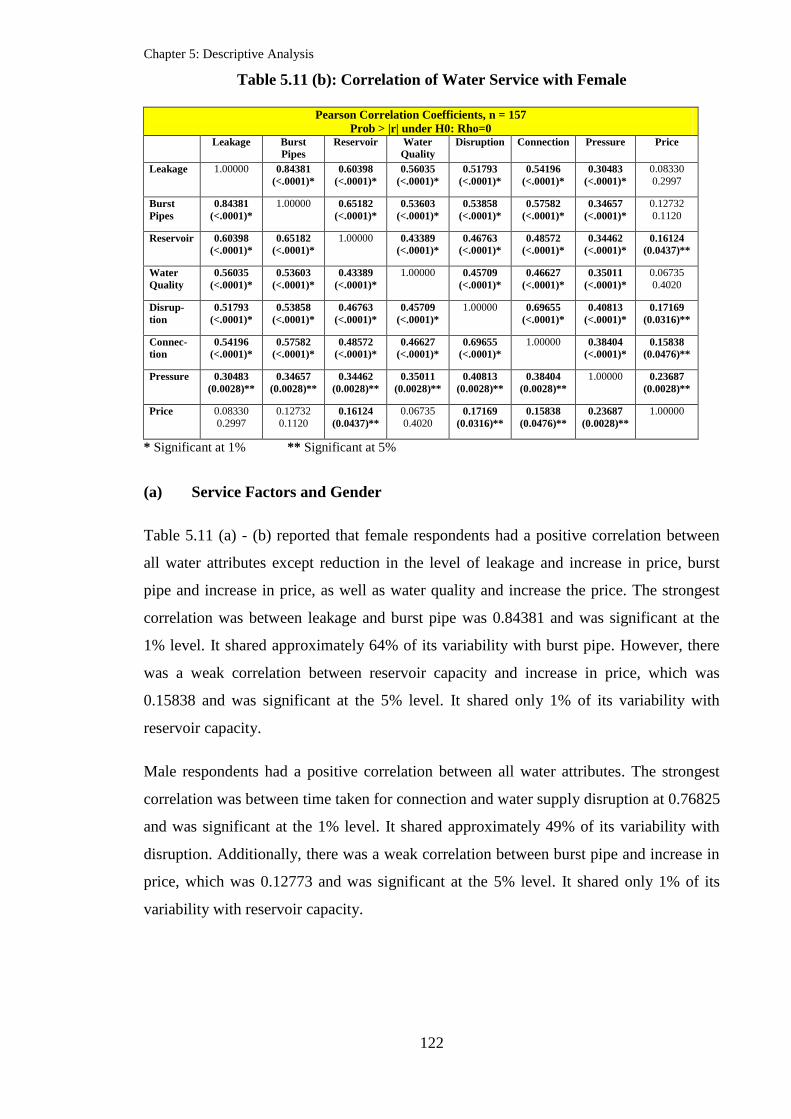
Chapter 5: Descriptive Analysis
122
Table 5.11 (b): Correlation of Water Service with Female
Pearson Correlation Coefficients, n = 157
Prob > |r| under H0: Rho=0 Leakage
Burst
Pipes
Reservoir Water
Quality
Disruption Connection Pressure Price
Leakage 1.00000 0.84381
(<.0001)*
0.60398
(<.0001)*
0.56035
(<.0001)*
0.51793
(<.0001)*
0.54196
(<.0001)*
0.30483
(<.0001)*
0.08330
0.2997
Burst
Pipes
0.84381
(<.0001)*
1.00000 0.65182
(<.0001)*
0.53603
(<.0001)*
0.53858
(<.0001)*
0.57582
(<.0001)*
0.34657
(<.0001)*
0.12732
0.1120
Reservoir 0.60398
(<.0001)*
0.65182
(<.0001)*
1.00000 0.43389
(<.0001)*
0.46763
(<.0001)*
0.48572
(<.0001)*
0.34462
(<.0001)*
0.16124
(0.0437)**
Water
Quality
0.56035
(<.0001)*
0.53603
(<.0001)*
0.43389
(<.0001)*
1.00000 0.45709
(<.0001)*
0.46627
(<.0001)*
0.35011
(<.0001)*
0.06735
0.4020
Disrup-
tion
0.51793
(<.0001)*
0.53858
(<.0001)*
0.46763
(<.0001)*
0.45709
(<.0001)*
1.00000 0.69655
(<.0001)*
0.40813
(<.0001)*
0.17169
(0.0316)**
Connec-
tion
0.54196
(<.0001)*
0.57582
(<.0001)*
0.48572
(<.0001)*
0.46627
(<.0001)*
0.69655
(<.0001)*
1.00000 0.38404
(<.0001)*
0.15838
(0.0476)**
Pressure 0.30483
(0.0028)**
0.34657
(0.0028)**
0.34462
(0.0028)**
0.35011
(0.0028)**
0.40813
(0.0028)**
0.38404
(0.0028)**
1.00000 0.23687
(0.0028)**
Price 0.08330
0.2997
0.12732
0.1120 0.16124
(0.0437)**
0.06735
0.4020 0.17169
(0.0316)**
0.15838
(0.0476)**
0.23687
(0.0028)**
1.00000
* Significant at 1% ** Significant at 5%
(a) Service Factors and Gender
Table 5.11 (a) - (b) reported that female respondents had a positive correlation between
all water attributes except reduction in the level of leakage and increase in price, burst
pipe and increase in price, as well as water quality and increase the price. The strongest
correlation was between leakage and burst pipe was 0.84381 and was significant at the
1% level. It shared approximately 64% of its variability with burst pipe. However, there
was a weak correlation between reservoir capacity and increase in price, which was
0.15838 and was significant at the 5% level. It shared only 1% of its variability with
reservoir capacity.
Male respondents had a positive correlation between all water attributes. The strongest
correlation was between time taken for connection and water supply disruption at 0.76825
and was significant at the 1% level. It shared approximately 49% of its variability with
disruption. Additionally, there was a weak correlation between burst pipe and increase in
price, which was 0.12773 and was significant at the 5% level. It shared only 1% of its
variability with reservoir capacity.

Chapter 5: Descriptive Analysis
123
Table 5.12 (a): Correlation of Water Service with Primary School
Spearman Correlation Coefficients, n = 39
Prob > |r| under H0: Rho=0
Leakage Burst Pipes Reservoir Water
Quality
Disruption Connection Pressure Price
Leakage 1.00000 0.95166
(<.0001)*
0.70504
(<.0001)*
0.59194
(<.0001)*
0.65792
(<.0001)*
0.48563
(0.0017)*
0.61839
(<.0001)*
0.16103 0.3274
Burst
Pipes
0.95166
(<.0001)*
1.00000 0.65388
(<.0001)*
0.55784
(0.0002)*
0.69592
(<.0001)*
0.52493
(0.0006)*
0.55819
(0.0002)**
0.12602
0.4446
Reservoir 0.70504
(<.0001)*
0.65388
(<.0001)*
1.00000 0.66200
(<.0001)*
0.65388
(<.0001)*
0.75651
(<.0001)*
0.70504
(<.0001)*
0.26469
0.1034
Water
Quality
0.59194
(<.0001)*
0.55784
(0.0002)**
0.66200
(<.0001)*
1.00000 0.55784
(0.0002)**
0.53119
(0.0005)**
0.49503
(0.0014)*
0.33383
(0.0378)**
Disrup-
tion
0.65792
(<.0001)*
0.69592
(<.0001)*
0.65388
(<.0001)*
0.55784
(0.0002)**
1.00000 0.80953
(<.0001)*
0.85193
(<.0001)*
0.40131
(0.0113)**
Connec-
tion
0.48563
(0.0017)*
0.52493
(0.0006)*
0.75651
(<.0001)*
0.53119
(0.0005)**
0.80953
(<.0001)*
1.00000 0.85690
(<.0001)*
0.30838
0.0561
Pressure 0.61839
(<.0001)*
0.55819
(0.0002)*
0.70504
(<.0001)*
0.49503
(0.0014)*
0.85193
(<.0001)*
0.85690
(<.0001)*
1.00000 0.31273
0.0526
Price 0.16103
0.3274
0.12602
0.4446
0.26469
0.1034
0.33383
(0.0378)**
0.40131
(0.0113)**
0.30838
0.0561
0.31273
0.0526
1.00000
* Significant at 1% ** Significant at 5%
Table 5.12 (b): Correlation of Water Service with Secondary School
Spearman Correlation Coefficients, n = 122
Prob > |r| under H0: Rho=0
Leakage Burst Pipes Reservoir Water
Quality
Disruption Connection Pressure Price
Leakage 1.00000 0.72401
(<.0001)*
0.68742
(<.0001)*
0.27501
(0.0022)*
0.53104
(<.0001)*
0.55621
(<.0001)*
0.39877
(<.0001)*
-0.03340 0.7150
Burst
Pipes
0.72401
(<.0001)*
1.00000 0.70766
(<.0001)*
0.30120
(0.0007)*
0.52254
(<.0001)*
0.54373
(<.0001)*
0.42476
(<.0001)*
0.01653
0.8566
Reservoir 0.68742
(<.0001)*
0.70766
(<.0001)*
1.00000 0.41478
(<.0001)*
0.58570
(<.0001)*
0.57517
(<.0001)*
0.44608
(<.0001)*
0.00633 0.9448
Water
Quality
0.27501
(0.0022)*
0.30120
(0.0007)*
0.41478
(<.0001)*
1.00000 0.32539
(0.0003)**
0.28455
(0.0015)*
0.31146
(0.0005)*
-0.06985 0.4445
Disrup-
tion
0.53104
(<.0001)*
0.52254
(<.0001)*
0.58570
(<.0001)*
0.32539
(0.0003)**
1.00000 0.66165
(<.0001)*
0.46544
(<.0001)*
0.09225
0.3122
Connec-
tion
0.55621
(<.0001)*
0.54373
(<.0001)*
0.57517
(<.0001)*
0.28455 0.0015
0.66165
(<.0001)*
1.00000 0.59825
(<.0001)*
0.09450 0.3005
Pressure 0.39877
(<.0001)*
0.42476
(<.0001)*
0.44608
(<.0001)*
0.31146 0.0005
0.46544
(<.0001)*
0.59825
(<.0001)*
1.00000 0.19966
(0.0275)**
Price
-0.03340 0.7150
0.01653 0.8566
0.00633 0.9448
-0.06985 0.4445
0.09225 0.3122
0.09450 0.3005
0.19966
(0.0275)**
1.00000
* Significant at 1% ** Significant at 5%

Chapter 5: Descriptive Analysis
124
Table 5.12 (c): Correlation of Water Service with College
Spearman Correlation Coefficients, n = 112
Prob > |r| under H0: Rho=0
Leakage Burst
Pipes
Reservoir Water
Quality
Disruptio
n
Connectio
n
Pressure Price
Leakage 1.00000 0.82124
(<.0001)*
0.76377
(<.0001)*
0.47450
(<.0001)*
0.76295
(<.0001)*
0.75613
(<.0001)*
0.50664
(<.0001)*
0.18765
(0.0476)**
Burst
Pipes
0.82124
(<.0001)*
1.00000 0.78804
(<.0001)*
0.45332
(<.0001)*
0.78977
(<.0001)*
0.74334
(<.0001)*
0.55517
(<.0001)*
0.12516 0.1886
Reser-
voir
0.76377
(<.0001)*
0.78804
(<.0001)*
1.00000 0.40949
(<.0001)*
0.73677
(<.0001)*
0.69702
(<.0001)*
0.58112
(<.0001)*
0.19303
(0.0414)**
Water
Quality
0.47450
(<.0001)*
0.45332
(<.0001)*
0.40949
(<.0001)*
1.00000 0.35605
(<.0001)*
0.47057
(<.0001)*
0.31702
(0.0007)*
0.01622
0.8652
Disrup-
tion
0.76295
(<.0001)*
0.78977
(<.0001)*
0.73677
(<.0001)*
0.35605
(<.0001)*
1.00000 0.78998
(<.0001)*
0.56475
(<.0001)*
0.14400 0.1298
Connec-
tion
0.75613
(<.0001)*
0.74334
(<.0001)*
0.69702
(<.0001)*
0.47057
(<.0001)*
0.78998
(<.0001)*
1.00000 0.60470
(<.0001)*
0.14248
0.1340
Pressure 0.50664
(<.0001)*
0.55517
(<.0001)*
0.58112
(<.0001)*
0.31702
(0.0007)*
0.56475
(<.0001)*
0.60470
(<.0001)*
1.00000 0.25874
(0.0059)*
Price
0.18765
(0.0476)**
0.12516
0.1886
0.19303
(0.0414)*
0.01622
0.8652
0.14400
0.1298
0.14248
0.1340 0.25874
(0.0059)*
1.00000
* Significant at 1% ** Significant at 5%
Table 5.12 (d): Correlation of Water Service with University
Spearman Correlation Coefficients, n = 118
Prob > |r| under H0: Rho=0
Leakage Burst
Pipes
Reservoir Water
Quality
Disruption Connection Pressure Price
Leakage 1.00000 0.82871
(<.0001)*
0.67227
(<.0001)*
0.42274
(<.0001)*
0.52262
(<.0001)*
0.55870
(<.0001)*
0.52982
(<.0001)*
0.03872 0.6772
Burst
Pipes
0.82871
(<.0001)*
1.00000 0.74769
(<.0001)*
0.36321
(<.0001)*
0.51872
(<.0001)*
0.63078
(<.0001)*
0.52830
(<.0001)*
0.08874
0.3393
Reser-
voir
0.67227
(<.0001)*
0.74769
(<.0001)*
1.00000 0.35812
(<.0001)*
0.56053
(<.0001)*
0.63095
(<.0001)*
0.55159
(<.0001)*
0.16263
0.0785
Water
Quality
0.42274
0.36321
(<.0001)*
0.35812
(<.0001)*
1.00000 0.45511
(<.0001)*
0.42162
(<.0001)*
0.45219
(<.0001)*
-0.06941
0.4552
Disrup-
tion
0.52262
(<.0001)*
0.51872
(<.0001)*
0.56053
(<.0001)*
0.45511
(<.0001)*
1.00000 0.72035
(<.0001)*
0.60800
(<.0001)*
0.08680
0.3500
Connec-
tion
0.55870
(<.0001)*
0.63078
(<.0001)*
0.63095
(<.0001)*
0.42162
(<.0001)
0.72035
(<.0001)
1.00000 0.61871
(<.0001)*
0.17557 0.0572
Pressure 0.52982
(<.0001)*
0.52830
(<.0001)*
0.55159
(<.0001)*
0.45219
(<.0001)*
0.60800
(<.0001)*
0.61871
(<.0001)*
1.00000 0.06413 0.4903
Price
0.03872
0.6772
0.08874
0.3393
0.16263
0.0785
-0.06941
0.4552
0.08680
0.3500
0.17557
0.0572
0.06413
0.4903
1.00000
* Significant at 1% ** Significant at 5%

Chapter 5: Descriptive Analysis
125
(b) Service Factors and Education
Table 5.12 (a) - (d) demonstrated that there was a positive correlation between some of
the water attributes for all levels of education. The strongest correlation was between
leakage and burst pipe at 0.95166 and was significant at the 1% level for those who only
went to primary school. It shared about 81% of its variability with burst pipe.
Additionally, it was followed by disruption and pressure, which was 0.85193 and was
significant at the 1% level. It shared approximately 64% of its variability with pressure.
Moreover, respondents who graduated from college and university had a strong
correlation between leakage and burst pipe, which were 0.82124 and 0.82871,
respectively. Both were significant at the 1% level. These attributes shared approximately
64% of their variability with burst pipe. For those educated to university level, there was
no correlation between an increase in the price and other attributes. Furthermore, the
weakest correlation was between an increase in the price and leakage for those who
studied at college. The coefficient was 0.18765 and was significant at the 5% level.
Table 5.13 (a): Correlation of Water Service with Support Staff
Spearman Correlation Coefficients, n =106
Prob > |r| under H0: Rho=0
Leakage Burst Pipes Reservoir Water
Quality
Disruption Connection Pressure Price
Leakage 1.00000 0.68925
(<.0001)*
0.61298
(<.0001)*
0.44998
(<.0001)*
0.52140
(<.0001)*
0.47984
(<.0001)*
0.22633
(0.0197)**
0.02425 0.8051
Burst
Pipes
0.68925
(<.0001)*
1.00000 0.62724
(<.0001)*
0.40668
(<.0001)*
0.54681
(<.0001)*
0.54965
(<.0001)*
0.25088
(0.0095)*
-0.06643
0.4987
Reservoir 0.61298
(<.0001)*
0.74769
(<.0001)*
1.00000 0.40784
(<.0001)*
0.58385
(<.0001)*
0.46914
(<.0001)*
0.33442
(0.0005)*
0.06839
0.4860
Water
Quality
0.44998
(<.0001)*
0.40668
(<.0001)*
0.40784
(<.0001)*
1.00000 0.39934
(<.0001)*
0.42331
(<.0001)*
0.25403
(0.0086)*
0.00021
0.9983
Disrup-
tion
0.52140
(<.0001)*
0.54681
(<.0001)*
0.58385
(<.0001)*
0.39934
(<.0001)*
1.00000 0.69388
(<.0001)*
0.50279
(<.0001)*
0.11672
0.2334
Connec-
tion
0.47984
(<.0001)*
0.54965
(<.0001)*
0.46914
(<.0001)*
0.42331
(<.0001)
0.69388
(<.0001)
1.00000 0.51358
(<.0001)*
0.18051 0.0641
Pressure 0.22633
(0.0197)**
0.25088
(0.0095)*
0.33442
(0.0005)*
0.25403
(0.0086)*
0.50279
(<.0001)*
0.51358
(<.0001)*
1.00000 0.33143
(0.0005)*
Price
0.02425 0.8051
-0.06643 0.4987
0.06839 0.4860
0.00021 0.9983
0.11672 0.2334
0.18051 0.0641
0.33143
(0.0005)*
1.00000
* Significant at 1% ** Significant at 5%

Chapter 5: Descriptive Analysis
126
Table 5.13 (b): Correlation of Water Service with Professional Staff
Spearman Correlation Coefficients, n = 106
Prob > |r| under H0: Rho=0
Leakage Burst Pipes Reservoir Water
Quality
Disruption Connection Pressure Price
Leakage 1.00000 0.90532
(<.0001)*
0.79976
(<.0001)*
0.29625
(0.0020)*
0.69708
(<.0001)*
0.73462
(<.0001)*
0.68184
(<.0001)*
0.13681 0.1620
Burst
Pipes
0.90532
(<.0001)*
1.00000 0.82466
(<.0001)*
0.21668
(0.0257)**
0.60368
(<.0001)*
0.75263
(<.0001)*
0.62612
(<.0001)*
0.23335
(0.0161)**
Reservoir 0.79976
(<.0001)*
0.82466
(<.0001)*
1.00000 0.31828
(0.0009)*
0.62062
(<.0001)*
0.74384
(<.0001)*
0.70019
(<.0001)*
0.20787
(0.0325)**
Water
Quality
0.29625
(0.0020)**
0.21668
(0.0257)**
0.31828
(0.0009)*
1.00000 0.38938
(<.0001)*
0.30952
(0.0012)*
0.39818
(<.0001)*
-0.02713
0.7825
Disrup-
tion
0.69708
(<.0001)*
0.60368
(<.0001)*
0.62062
(<.0001)*
0.38938
(<.0001)*
1.00000 0.70239
(<.0001)*
0.66852
(<.0001)*
0.11716 0.2317
Connec-
tion
0.73462
(<.0001)*
0.75263
(<.0001)*
0.74384
(<.0001)*
0.30952
(0.0012)*
0.70239
(<.0001)
1.00000 0.72755
(<.0001)*
0.25541
(0.0082)*
Pressure 0.68184
(<.0001)*
0.62612
(<.0001)*
0.70019
(<.0001)*
0.39818
(<.0001)*
0.66852
(<.0001)*
0.72755
(<.0001)*
1.00000 0.14231
0.1456
Price 0.13681
0.1620
0.23335
(0.0161)**
0.20787
(0.0325)**
-0.02713
0.7825
0.11716
0.2317 0.25541
(0.0082)*
0.14231
0.1456
1.00000
* Significant at 1% ** Significant at 5%
Table 5.13 (c): Correlation of Water Service with Others
Spearman Correlation Coefficients, n = 179
Prob > |r| under H0: Rho=0
Leakage Burst
Pipes
Reservoir Water
Quality
Disruption Connection Pressure Price
Leakage 1.00000 0.81947
(<.0001)*
0.71088
(<.0001)*
0.61312
(<.0001)*
0.62338
(<.0001)*
0.62338
(<.0001)*
0.54379
(<.0001)*
0.05335
0.4781
Burst
Pipes
0.82871
(<.0001)*
1.00000 0.74498
(<.0001)*
0.47696
(<.0001)*
0.66145
(<.0001)*
0.60522
(<.0001)*
0.59559
(<.0001)*
0.07431
0.3228
Reservoir 0.71088
(<.0001)*
0.74498
(<.0001)*
1.00000 0.48517
(<.0001)*
0.65289
(<.0001)*
0.69822
(<.0001)*
0.57145
(<.0001)*
0.12195
0.1039
Water
Quality
0.44167
(<.0001)*
0.47696
(<.0001)*
0.48517
(<.0001)*
1.00000 0.42632
(<.0001)*
0.43320
(<.0001)*
0.41754
(<.0001)*
-0.00146
0.9846
Disrup-
tion
0.61312
(<.0001)*
0.66145
(<.0001)*
0.65289
(<.0001)*
0.42632
(<.0001)*
1.00000 0.75457
(<.0001)*
0.54772
(<.0001)*
0.12960
0.0838
Connec-
tion
0.62338
(<.0001)*
0.60522
(<.0001)*
0.69822
(<.0001)*
0.43320
(<.0001)
0.75457
(<.0001)
1.00000 0.62241
(<.0001)*
0.07153 0.3413
Pressure 0.54379
(<.0001)*
0.59559
(<.0001)*
0.57145
(<.0001)*
0.41754
(<.0001)*
0.54772
(<.0001)*
0.62241
(<.0001)*
1.00000 0.13337 0.0751
Price
0.05335
0.4781
0.07431
0.3228
0.12195
0.1039
-0.00146
0.9846
0.12960
0.0838
0.07153
0.3413
0.13337
0.0751
1.00000
* Significant at 1% ** Significant at 5%

Chapter 5: Descriptive Analysis
127
(c) Service Factors and Work
Table 5.13 (a) - (c) revealed that professional respondents have a positive correlation
between some of the water attributes. The strongest correlation was between leakage and
burst pipe, which was 0.90532 and was significant at the 1% level. It shared
approximately 64% of its variability with burst pipe. The weakest correlation was
between increase in price and reservoir capacity, which was 0.20787 and was significant
at the 5% level.
Furthermore, for the “others” group, there were correlations with all water attributes
except increase in price. Similarly, the strongest correlation was between leakage and
burst pipe, which was 0.81947 and was significant at the 1% level. It shared
approximately 64% of its variability with improve repairs to burst pipe. Meanwhile, in the
support staff group, the strongest correlation was between disruption and time taken for
connection. The coefficient was 0.69388 and was significant at the 1% level. It shared
approximately 49% of its variability with time taken for connection.
Table 5.14 (a): Correlation of Water Service with Income (MYR500 or less per
month)
Pearson Correlation Coefficients, n = 42
Prob > |r| under H0: Rho=0
Leakage Burst
Pipes
Reservoir Water
Quality
Disruption Connection Pressure Price
Leakage 1.00000 0.77071
(<.0001)*
0.55392
(<.0001)*
0.57826
(<.0001)*
0.58780
(<.0001)*
0.54220
(0.0002)*
0.65458
(<.0001)*
0.29255
0.0601
Burst
Pipes
0.77071
(<.0001)*
1.00000 0.72731
(<.0001)*
0.61497
(<.0001)*
0.66560
(<.0001)*
0.67361
(<.0001)*
0.70159
(<.0001)*
0.41747
(0.0059)*
Reser-
voir
0.55392
(<.0001)*
0.72731
(<.0001)*
1.00000 0.60228
(<.0001)*
0.63539
(<.0001)*
0.72749
(<.0001)*
0.70605
(<.0001)*
0.17411 0.2701
Water
Quality
0.57826
(<.0001)*
0.61497
(<.0001)*
0.60228
(<.0001)*
1.00000 0.67008
(<.0001)*
0.59249
(<.0001)*
0.60384
(<.0001)*
0.18789 0.2334
Disrup-
tion
0.58780
(<.0001)*
0.66560
(<.0001)*
0.63539
(<.0001)*
0.67008
(<.0001)*
1.00000 0.82263
(<.0001)*
0.75190
(<.0001)*
0.27164
0.0818
Connec-
tion
0.54220
(0.0002)*
0.67361
(<.0001)*
0.72749
(<.0001)*
0.59249
(<.0001)
0.82263
(<.0001)
1.00000 0.79483
(<.0001)*
0.25243
0.1068
Pressure 0.65458
(<.0001)*
0.70159
(<.0001)*
0.70605
(<.0001)*
0.60384
(<.0001)*
0.75190
(<.0001)*
0.79483
(<.0001)*
1.00000 0.27968
0.0728
Price
0.29255
0.0601
0.41747
(0.0059)*
0.17411
0.2701
0.18789
0.2334
0.27164
0.0818
0.25243
0.1068
0.27968
0.0728
1.00000
*Significant at 1% **Significant at 5%

Chapter 5: Descriptive Analysis
128
Table 5.14 (b): Correlation of Water Service with Income (MYR500–MYR1,500 per
month)
Pearson Correlation Coefficients, n = 105
Prob > |r| under H0: Rho=0
Leakage Burst Pipes Reservoir Water
Quality
Disruption Connection Pressure Price
Leakage 1.00000 0.77144
(<.0001)*
0.73444
(<.0001)*
0.54859
(<.0001)*
0.59595
(<.0001)*
0.58676
(0.0002)*
0.47135
(<.0001)*
0.09823 0.3188
Burst
Pipes
0.77144
(<.0001)*
1.00000 0.65464
(<.0001)*
0.59943
(<.0001)*
0.61290
(<.0001)*
0.54370
(<.0001)*
0.50300
(<.0001)*
0.04241
0.6675
Reservoir 0.73444
(<.0001)*
0.65464
(<.0001)*
1.00000 0.48705
(<.0001)*
0.65747
(<.0001)*
0.59436
(<.0001)*
0.49947
(<.0001)*
0.20434
(0.0365)**
Water
Quality
0.54859
(<.0001)*
0.59943
(<.0001)*
0.48705
(<.0001)*
1.00000 0.49665
(<.0001)*
0.56323
(<.0001)*
0.41059
(<.0001)*
0.10726
0.2761
Disrup-
tion
0.59595
(<.0001)*
0.61290
(<.0001)*
0.65747
(<.0001)*
0.49665
(<.0001)*
1.00000 0.79224
(<.0001)*
0.42756
(<.0001)*
0.1506
0.1250
Connec-
tion
0.58676
(0.0001)*
0.54370
(<.0001)*
0.59436
(<.0001)*
0.56323
(<.0001)
0.79224
(<.0001)
1.00000 0.43258
(<.0001)*
0.1615
0.1068
Pressure 0.47135
(<.0001)*
0.50300
(<.0001)*
0.49947
(<.0001)*
0.41059
(<.0001)*
0.42756
(<.0001)*
0.43258
(<.0001)*
1.00000 0.23612
(0.0153)**
Price
0.09823 0.3188
0.04241
0.6675
0.20434 0.0365
0.10726 0.2761
0.15067 0.1250
0.16157 0.0996
0.23612
(0.0153)**
1.00000
*Significant at 1% **Significant at 5%
Table 5.14 (c): Correlation of Water Service with Income (MYR1501–MYR2,500
per month)
Pearson Correlation Coefficients, n = 133
Prob > |r| under H0: Rho=0
Leakage Burst Pipes Capacity Water
Quality
Disruption Connection Pressure Price
Leakage 1.00000 0.73043 0.58004 0.46440 0.61969 0.63736 0.34470 0.14291
(<.0001)*
(<.0001)* (<.0001)* (<.0001)* (<.0001)* (<.0001)* 0.1008
Burst pipe 0.73043 1.00000 0.69735 0.52041 0.61906 0.66151 0.33174 0.16440
(<.0001)*
(<.0001)* (<.0001)* (<.0001)* (<.0001)* (<.0001)* 0.0586
Reservoir 0.58004 0.69735 1.00000 0.47556 0.61130 0.50210 0.29290 0.20150
(<.0001)*
(<.0001)* (<.0001)* (<.0001)* (<.0001)* (0.0006)* (0.0200)**
Water
Quality
0.46440
(<.0001)*
0.52041
(<.0001)*
0.47556
(<.0001)*
1.00000 0.45700
(<.0001)*
0.46416
(<.0001)*
0.31412
(0.0002)*
0.08014 0.3592
Disrup-
tion
0.61969 0.61906 0.61130 0.45700 1.00000 0.69490 0.41037 0.21356
(<.0001)* (<.0001)* (<.0001)* (<.0001)*
(<.0001)* (<.0001)* (0.0136)**
Connec-
tion
0.63736 0.66151 0.50210 0.46416 0.69490 1.00000 0.40074 0.20974
(<.0001)*
(<.0001)* (<.0001)* (<.0001)* (<.0001)* (<.0001)* (0.0154)**
Pressure 0.34470 0.33174 0.29290 0.31412 0.41037 0.40074 1.00000 0.35454
(<.0001)*
(<.0001)* (0.0006)* (0.0002)* (<.0001)* (<.0001)* (<.0001)*
Price 0.14291 0.16440 0.20150 0.08014 0.21356 0.20974 0.35454 1.00000 0.1008 0.0586 (0.0200)** 0.3592 (0.0136)** (0.0154)** (<.0001)*
*Significant at 1% **Significant at 5%

Chapter 5: Descriptive Analysis
129
Table 5.14 (d): Correlation of Water Service with Income (more than MYR2,501 per
month)
Pearson Correlation Coefficients, n = 112
Prob > |r| under H0: Rho=0
Leakage Burst Pipes Reservoir Water
Quality
Disruption Connection Pressure Price
Leakage 1.00000 0.84172
(<.0001)*
0.55968
(<.0001)*
0.30846
(0.0009)*
0.59595
(<.0001)*
0.54720
(<.0001)*
0.30807
(0.0010)*
0.08301 0.3842
Burst
Pipes
0.84172
(<.0001)*
1.00000 0.59291
(<.0001)*
0.34610
(<.0002)*
0.61290
(<.0001)*
0.59435
(<.0001)*
0.35427
(<.0001)*
0.07185 0.4515
Reservoir 0.55968
(<.0001)*
0.59291
(<.0001)*
1.00000 0.14106
0.1379
0.30792
(<.0010)*
0.45908
(<.0001)*
0.34281
(<.0002)*
0.12628
0.1846
Water
Quality
0.30846
(0.0009)*
0.34610
(<.0002)*
0.14106
0.1379
1.00000 0.26471
(0.0048)*
0.18990
(0.0449)**
0.20815
(0.0276)**
-0.07945
0.4050
Disrup-
tion
0.52343
(<.0001)*
0.56720
(<.0001)*
0.30792
(<.0010)*
0.26471
(0.0048)**
1.00000 0.65855
(<.0001)*
0.40741
(<.0001)*
0.17795
0.0605
Connec-
tion
0.54720
(0.0001)*
0.59435
(<.0001)*
0.45908
(<.0001)*
0.18990
(0.0449)**
0.65855
(<.0001)
1.00000 0.51415
(<.0001)*
0.18708
(0.0483)**
Pressure 0.30807
(<.0010)*
0.35427
(<.0001)*
0.34281
(<.0002)*
0.20815
(0.0276)**
0.40741
(<.0001)*
0.51415
(<.0001)*
1.00000 0.04943
0.6048
Price
0.08301 0.3842
0.07185 0.4515
0.12628 0.1846
-0.07945 0.4050
0.17795 0.0605
0.18708
(0.0483)**
0.04943 0.6048
1.00000
*Significant at 1% **Significant at 5%
(d) Service Factors and Income
Table 5.14 (a) - (d) revealed that there was a positive correlation between some of the
water attributes. The strongest correlation was between leakage and burst pipe at 0.84172
and was significant at the 1% level. It shared approximately 64% of its variability with
burst pipe for those with an income of more than MYR2,501 per month. It was followed
by those with an income of MYR500 or less per month; the strongest relationship was
between disruption and time taken for connection, which was 0.82263 and was significant
at the 1% level. It shared approximately 64% of its variability with time taken for
connection. Similarly, the coefficient for respondents who had an income of MYR501 to
MYR1,500 was 0.79224. The weakest correlation was between increase in price and burst
pipe, which was 0.41747 and was significant at the 1% level.
5.9.3 Correlation Perceptions of Improvement of Strategies and Socioeconomics
The results of the correlation between perception of improvement of strategies and
socioeconomics have been presented as follows:

Chapter 5: Descriptive Analysis
130
Table 5.15 (a): Correlation of Strategies with Male
Pearson Correlation Coefficients, n = 235
Prob > |r| under H0: Rho=0
Integrated Training Funding Education
Integrated 1.00000 0.74319 0.71881 0.70575
(<.0001)* (<.0001)* (<.0001)*
Training 0.74319 1.00000 0.73084 0.77722
(<.0001)* (<.0001)* (<.0001)*
Funding 0.71881 0.73084 1.00000 0.74902
(<.0001)* (<.0001)* (<.0001)*
Education 0.70575 0.77722 0.74902 1.00000
(<.0001)* (<.0001)* (<.0001)*
* Significant at 1%
Table 5.15 (b): Correlation of Strategies with Female
Pearson Correlation Coefficients, n = 157
Prob > |r| under H0: Rho=0
Integrated Training Funding Education
Integrated 1.00000 0.55820 0.57841 0.62713
(<.0001)* (<.0001)* (<.0001)*
Training 0.55820 1.00000 0.60585 0.47806
(<.0001)* (<.0001)* (<.0001)*
Funding 0.57841 0.60585 1.00000 0.67854
(<.0001)* (<.0001)* (<.0001)*
Education 0.62713 0.47806 0.67854 1.00000
(<.0001)* (<.0001)* (<.0001)*
* Significant at 1%
(a) Improvement of Strategies and Gender
Table 5.15 (a) - (b) showed that there was a positive correlation between all improvement
strategies. For male respondents, the strongest relation was between providing good
quality training to all staff and encouraging education and awareness, which was 0.77722
and was significant at the 1% level. It shared approximately 49% of its variability with
encouraging education and awareness. It was followed by the correlation between funding
for new investment and encouraging education and awareness. The coefficient was
0.74902 and was significant at the 1% level. It shared approximately 49% of its
variability with encouraging education and awareness. With female respondents, there
was a correlation between funding for new investment and encouraging education and

Chapter 5: Descriptive Analysis
131
awareness, which was 0.67854 and was significant at the 1% level. It shared
approximately 36% of its variability with encouraging education and awareness.
Table 5.16 (a): Correlation of Strategies with Primary School
Spearman Correlation Coefficients, n = 39
Prob > |r| under H0: Rho=0
Integrated Training Funding Education
Integrated 1.00000 0.69629 0.74363 0.80829
(<.0001)* (<.0001)* (<.0001)*
Training 0.69629 1.00000 0.95004 0.73458
(<.0001)* (<.0001)* (<.0001)*
Funding 0.74363 0.95004 1.00000 0.68825
(<.0001)* (<.0001)* (<.0001)*
Education 0.80829 0.73458 0.68825 1.00000
(<.0001)* (<.0001)* (<.0001)*
*Significant at 1%
Table 5.16 (b): Correlation of Strategies with Secondary School
Spearman Correlation Coefficients, n = 122
Prob > |r| under H0: Rho=0
Integrated Training Funding Education
Integrated 1.00000 0.73965 0.79292 0.73965
(<.0001)* (<.0001)* (<.0001)*
Training 0.73965 1.00000 0.74485 0.62500
(<.0001)* (<.0001)* (<.0001)*
Funding 0.79292 0.74485 1.00000 0.74589
(<.0001)* (<.0001)* (<.0001)*
Education 0.73965 0.62500 0.74589 1.00000
(<.0001)* (<.0001)* (<.0001)*
*Significant at 1%

Chapter 5: Descriptive Analysis
132
Table 5.16 (c): Correlation of Strategies with College
Spearman Correlation Coefficients, n = 112
Prob > |r| under H0: Rho=0
Integrated Training Funding Education
Integrated 1.00000 0.75219 0.75996 0.78132
(<.0001)* (<.0001)* (<.0001)*
Training 0.75219 1.00000 0.74239 0.78145
(<.0001)* (<.0001)* (<.0001)*
Funding 0.75996 0.74239 1.00000 0.85655
(<.0001)* (<.0001)* (<.0001)*
Education 0.78132 0.78145 0.85655 1.00000
(<.0001)* (<.0001)* (<.0001)*
*Significant at 1%
Table 5.16 (d): Correlation of Strategies with University
Spearman Correlation Coefficients, n = 118
Prob > |r| under H0: Rho=0
Integrated Training Funding Education
Integrated 1.00000 0.65294 0.65908 0.59097
(<.0001)* (<.0001)* (<.0001)*
Training 0.65294 1.00000 0.57213 0.71851
(<.0001)* (<.0001)* (<.0001)*
Funding 0.65908 0.57213 1.00000 0.65513
(<.0001)* (<.0001)* (<.0001)*
Education 0.59097 0.71851 0.65513 1.00000
(<.0001)* (<.0001)* (<.0001)*
*Significant at 1%
(b) Improvement of Strategies and Education
Table 5.16 (a) - (d) demonstrated that there was a positive correlation between all
improvement strategies. The strongest correlation was between providing good quality
training to all staff and increasing funding for new investment, which was 0.95004 and
was significant at the 1% level for those who only studied in primary school. It shared
approximately 81% of its variability with funding for new investment. Furthermore, it
was followed by funding for new investment and encouraging education and awareness at
0.85655, which was significant at the 1% level for those who graduated from college. It
shared approximately 64% of its variability with encouraging education and awareness.
Surprisingly, for respondents who had graduated from university, there was a low
correlation between providing good quality training to all staff and encouraging education

Chapter 5: Descriptive Analysis
133
and awareness, which was 0.71851 and significant at the 1% level. It shared
approximately 49% of its variability with encouraging education and awareness.
Table 5.17 (a): Correlation of Strategies with Support Staff
Spearman Correlation Coefficients, n = 106
Prob > |r| under H0: Rho=0
Integrated Training Funding Education
Integrated 1.00000 0.78621 0.69904 0.67835
(<.0001)* (<.0001)* (<.0001)*
Training 0.78621 1.00000 0.71429 0.66172
(<.0001)* (<.0001)* (<.0001)*
Funding 0.69904 0.71429 1.00000 0.76800
(<.0001)* (<.0001)* (<.0001)*
Education 0.67835 0.66172 0.76800 1.00000
(<.0001)* (<.0001)* (<.0001)*
*Significant at 1%
Table 5.17 (b): Correlation of Strategies with Professional
Spearman Correlation Coefficients, n = 106
Prob > |r| under H0: Rho=0
Integrated Training Funding Education
Integrated 1.00000 0.69778 0.82800 0.75446
(<.0001)* (<.0001)* (<.0001)*
Training 0.69778 1.00000 0.69438 0.74935
(<.0001)* (<.0001)* (<.0001)*
Funding 0.82800 0.69438 1.00000 0.78304
(<.0001)* (<.0001)* (<.0001)*
Education 0.75446 0.74935 0.78304 1.00000
(<.0001)* (<.0001)* (<.0001)*
*Significant at 1%

Chapter 5: Descriptive Analysis
134
Table 5.17 (c): Correlation of Strategies with Others
Spearman Correlation Coefficients, n = 179
Prob > |r| under H0: Rho=0
Integrated Training Funding Education
Integrated 1.00000 0.67920 0.69952 0.70052
(<.0001)* (<.0001)* (<.0001)*
Training 0.67920 1.00000 0.71970 0.71483
(<.0001)* (<.0001)* (<.0001)*
Funding 0.69952 0.71970 1.00000 0.70003
(<.0001)* (<.0001)* (<.0001)*
Education 0.70052 0.71483 0.70003 1.00000
(<.0001)* (<.0001)* (<.0001)*
*Significant at 1%
(c) Improvement of Strategies and Work
Table 5.17 (a) - (c) showed that there was a positive correlation between all improvement
strategies. For respondents who work as professional staff, the strongest correlation was
between an integrated strategic plan and funding for new investment, which was 0.82800
and was significant at the 1% level. It shared about 64% of its variability with increase
funding for new investment. This was followed, by a correlation between an integrated
strategic plan and providing good quality training to all staff for those who worked as
support staff. The coefficient was 0.78621 and was significant at the 1% level. It shared
approximately 64% of its variability with providing good quality training to all staff.
Table 5.18 (a): Correlation of Strategies and Income (MYR500 or less per month)
Pearson Correlation Coefficients, n = 42
Prob > |r| under H0: Rho=0
Integrated Training Funding Education
Integrated 1.00000 0.67797 0.62573 0.69039
(<.0001)* (<.0001)* (<.0001)*
Training 0.67797 1.00000 0.67904 0.69952
(<.0001)* (<.0001)* (<.0001)*
Funding 0.62573 0.67904 1.00000 0.67864
(<.0001)* (<.0001)* (<.0001)*
Education 0.69039 0.69952 0.67864 1.00000
(<.0001)* (<.0001)* (<.0001)*
*Significant at 1%

Chapter 5: Descriptive Analysis
135
Table 5.18 (b): Correlation of Strategies and Work (MYR501–MYR1,500 per
month)
Pearson Correlation Coefficients, n = 105
Prob > |r| under H0: Rho=0
Integrated Training Funding Education
Integrated 1.00000 0.55875 0.58454 0.69784
(<.0001)* (<.0001)* (<.0001)*
Training 0.55875 1.00000 0.62461 0.52755
(<.0001)* (<.0001)* (<.0001)*
Funding 0.58454 0.62461 1.00000 0.62631
(<.0001)* (<.0001)* (<.0001)*
Education 0.69784 0.52755 0.62631 1.00000
(<.0001)* (<.0001)* (<.0001)*
*Significant at 1%
Table 5.18 (c): Correlation of Strategies and Work (MYR1,501–MYR2,500 per
month)
Pearson Correlation Coefficients, n = 132
Prob > |r| under H0: Rho=0
Integrated Training Funding Education
Integrated 1.00000 0.56723 0.65603 0.61697
(<.0001)* (<.0001)* (<.0001)*
Training 0.56723 1.00000 0.66622 0.63809
(<.0001)* (<.0001)* (<.0001)*
Funding 0.65603 0.66622 1.00000 0.64881
(<.0001)* (<.0001)* (<.0001)*
Education 0.61697 0.63809 0.64881 1.00000
(<.0001)* (<.0001)* (<.0001)*
*Significant at 1%

Chapter 5: Descriptive Analysis
136
Table 5.18 (d): Correlation of Strategies and Work (More than MYR2,501 per
month)
Pearson Correlation Coefficients, n = 122
Prob > |r| under H0: Rho=0
Integrated Training Funding Education
Integrated 1.00000 0.84675 0.75261 0.70406
(<.0001)* (<.0001)* (<.0001)*
Training 0.84675 1.00000 0.74382 0.75550
(<.0001)* (<.0001)* (<.0001)*
Funding 0.75261 0.74382 1.00000 0.88501
(<.0001)* (<.0001)* (<.0001)*
Education 0.70406 0.75550 0.88501 1.00000
(<.0001)* (<.0001)* (<.0001)*
*Significant at 1%
(d) Improvement of Strategies and Income
Table 5.18 (a) - (d) revealed that there was a positive correlation between all
improvement strategies. The strongest correlation was between funding for new
investment and encouraging education and awareness, which was 0.88501 and was
significant at the 1% level. It shared approximately 64% of its variability with
encouraging education and awareness for those who had an income of more than
MYR2,501 per month. This was followed by the correlation between providing good
quality training to all staff and an integrated strategic plan. The coefficient was 0.84675
and shared approximately 64% of its variability with an integrated strategic plan.
Additionally, for those who had an income of MYR501 to MYR1,500 per month, the
strongest relationship was between an integrated strategic plan and encouraging education
and awareness, which was 0.69784 and was significant at the 1% level. It shared
approximately 49% of its variability with encouraging education and awareness. The
weakest correlation was between encouraging education and awareness and providing
good quality training to all staff, which was 0.52755 and was significant at the 1% level.
5.10 Conclusions
The sample size was 392 respondents. It covered three districts in Johor: Kluang, Batu
Pahat and Johor Bahru. The majority of respondents have been with SAJH since
privatisation (March 2000) to the present day. Socioeconomics are considered one of the
factors which influence WTP for improvements to service quality.

Chapter 5: Descriptive Analysis
137
Water quality achieved 98% compliance to MOH Standards. Due to old water pipes and
customer concern about the safety of drinking water, the results showed that most of the
respondents used a water filter at home (44.64%) and bought mineral or bottled water for
drinking at home (53.06%).
Performance of service quality measured leakage, pipe bursts, reservoirs, water quality
standards, disruption, connections, pressure, and price. The results indicated that more
that 50% of respondents were satisfied with service quality. However, the service needs
to be upgraded and improved because certain attributes did not achieve 100% of satisfied
respondents.
In order to improve the service quality, the results showed that a majority of respondents
agreed the importance of strategies consisting of reducing leakage, improving the
repairing of burst pipes, increasing reservoirs‟ capacity, improving the water quality,
reducing water supply disruptions, improving the time taken for connections to the water
supply, and increasing the water pressure level.
Furthermore, more than 90% of respondents agreed with the strategies that included
setting up an integrated strategic plan, providing good quality training to staff, increasing
funding for new investment, and encouraging education and awareness about upgrading
the service quality to achieve excellence in the future.
The cross tabulation findings between the perception on service quality performance,
improvement of water service and improvement of strategies, and socioeconomic
characteristics demonstrated that most of the respondents were satisfied with those
aspects. The majority of respondents (approximately 50%) were male and the majority
were Malay. The most common age group was between 20 to 30 years old. About 40% of
respondents had two children or fewer. This was followed by respondents with three to
five children (approximately 25%). 30% of respondents had six to eight persons in their
households. The majority of respondents lived in terraced or two-storey houses.
Furthermore, most of the respondents had qualifications from college or university. The
majority of respondents worked as self-employed, followed by the professional group at
about 20%. The most common income groups were those who earned between
MYR1,501 and MYR2,500 per month and those who earned more than MYR2,501 per
month. It is interesting to observe preferences for certain attributes based on the

Chapter 5: Descriptive Analysis
138
socioeconomic characteristics of the consumer. Therefore, the water company should
consider customer preferences with regard to the water attributes and socioeconomics in
order to better satisfy and fulfil the customers‟ wishes.
Furthermore, the results of the correlation analysis revealed that there was a positive
relationship between the majority of attributes of service quality performance. There was
also a strong correlation among attributes as well as the attributes of the improvement of
the water service. Only the attribute price has a weak correlation with the other water
attributes. Furthermore, the results showed that there was a positive and strong correlation
between all improvement strategies. For instance, the level of education was the most
important variable that influenced the WTP. Therefore, the respondents who have a
higher level of education are more likely to satisfy the more reduction of leakage for
upgrading the water service. Therefore, this pattern of relationships is meaningful to
determine the priority of water attributes and socioeconomic characteristics in order to
deliver an excellent water service.
In conclusion, the descriptive analysis, including cross tabulation and correlation analysis,
found that there were priority aspects of the service quality and the pattern of
socioeconomics which should be considered and improved by SAJH.

Chapter 6: Choice Experiment Results
139
CHAPTER 6: CHOICE EXPERIMENT RESULTS
6.1 Introduction
This chapter reports the results of the choice experiment for the water supply service of
Johor Water Company (SAJH). It begins by documenting the responses to the choice
experiment cards. The chapter then presents results for the first choice experiment: Water
Infrastructure (WI). A number of different models are used, namely: (i) the basic
conditional logit (CL) model; (ii) CL with an alternative specific constant for the status
quo or current position (asc0); (iii) CL with non-linear terms, (iv) CL with non-linear
terms and asc0; and (v) CL incorporating levels. These models are then extended to
include CL models with interaction terms with socioeconomic characteristics, and the
mixed logit model (in Chapter7). This chapter also reports on a second choice
experiment: Residential Customers (RC), comprising a similar series to the models
already mentioned, except for CL with asc0, CL with non-linear terms and asc0, and CL
incorporating levels.
6.2 Pattern of Responses
Both of the choice experiments, Water Infrastructure (WI) and Residential Customers
(RC), comprised a number of attributes. The four attributes of the WI choice experiment
were leakage (LEA), burst pipe (BUR), reservoirs (RES), and price (PRI). The five
attributes of the RC choice experiment consisted of water quality standard (QUA),
disruption (DIS), connection (CON), pressure (PRE) and price (PRI). Table 6.1 reports
the pattern of attribute levels on the choice cards that were presented to respondents.
Most choice cards showed a preferred leakage level of a decrease by 20%. This occurred
on 41.65% of the cards. This was followed by the current situation, estimated at 33.35%.
The choices for BUR the current situation and an improvement of repairing 100% of
bursts within 24 hours – were approximately 50% and 41.67%, respectively. A small
percentage chose an increase to 99.9%. In terms of reservoir capacity (RES), most
respondents chose the current situation, i.e. „no change‟: this appeared on 66.67% of the
cards. This was followed by 25.02% of customers choosing a RES increase to 125%.

Chapter 6: Choice Experiment Results
140
Attributes Description (unit) Descriptive Statistics Freq (%) Mean St.
Dev
Min Max
Water Infrastructure (WI): N = 4704
LEA Leakage (% change) 25.41 4.31 20.00 30.00
a) 30% 1569 (33.35)
b) decrease to 25% 1176 (25.00)
c) decrease to 20% 1959 (41.65)
BUR Burst Pipe (% change) 99.16 0.71 98.50 100.00
a) 98.5% 2352 (50.00)
b) increase to 99.0% 392 (8.33)
c) increase to 100% 1960 (41.67)
RES Reservoir (% change) 121.41 9.24 119.00 130.00
a) 119% 3136 (66.67)
b) increase to 125% 1177 (25.02)
c) increase to 130% 391 (8.31)
PRI Price (% change) 7.50 9.24 0.00 20.00
a) no change 2744 (58.33)
b) increase of 10% 391 (8.31)
c) increase of 20% 1569 (33.35)
Residential Customers (RC): N = 4704
QUA Water Quality (% change) 99.75 0.07 99.70 99.90
a) 99.7% 2744 (58.33)
b) increase to 99.8% 1176 (25.00)
c) increase to 99.9% 786 (16.67)
DIS Disruption 1.82 0.57 1.20 2.40
a) 2 hours per day
for 4 days a year
1176 (25.00)
b) 2 hours per day
for 3 days a year
1176 (25.00)
c) 1 hour per day
for 2 days a year
2352 (50.00)
CON Connection 2.58 0.64 1.00 3.00
a) 3 days 392 (8.33)
b) decrease to 2
days
1176 (25.00)
c) decrease to 1 day 3136 (66.67)
PRE Pressure (% change) 94.91 1.97 93.00 98.00
a) 93% 1960 (41.67)
b) increase to 95% 1568 (33.33)
c) increase to 98% 1176 (25.00)
PRI Price (% change) 6.66 7.45 0.00 20.00
a) no change 2352 (50.00)
b) increase by 10% 1568 (33.33)
c) increase by 20% 784 (16.67)
Most of the choice cards expressed a preference for the current situation of water quality
(QUA) (58.33%). Obviously, where the quality level choice was increased to 99.9%, the
number of choice cards selected was decreased: the percentage was approximately
16.67% of responses for this alternative. Both disruption (DIS) and connection (CON)
saw most of the choice cards selected improving the disruption period to one hour per day
Table 6.1: Descriptions and Descriptive Statistics of the Main Attributes for the
Choice Experiment

Chapter 6: Choice Experiment Results
141
for two days a year and decreasing the connection time to one day: 50% and 66.67%,
respectively. In terms of pressure (PRE), the preferred option was the current situation:
the percentage was 41.67%. When the percentage of PRE increased, the number of choice
cards declined, so that a PRE increase to 98% only scored 25%.
In terms of price (PRI) it is apparent that most preferred the selection of the current price,
i.e.. „no change‟. In the WI experiment, approximately 58% of all choices were for „no
change‟ in price; and in the RC experiment this percentage was 50%. In the RC
experiment it was clear that as price increased, the number of times respondents selected
this option decreased, so that a 20% price increase only attracted 16.6% of responses.
In order to further explain the CL model, the theoretical expectation of the attributes of
WI and RC are stated in Table 6.2. Basically, the customer chooses the alternative that
provides the greatest utility. In Part 1, BUR and RES are expected to be positive signs;
whilst LEA and PRI are expected to have negative signs. It means that customers will
gain more utility with a decrease in the percentage of LEA and PRI. Meanwhile,
customers will entertain more utility with an increase in the percentage of BUR and RES.
Furthermore, QUA and PRE will be expected to be positive signs; DIS, CON and PRI,
negative signs. Customers‟ utility will increase with a decrease in the percentage of DIS,
CON, and PRI. However, increasing the percentage of QUA and PRE will cause a rise of
customers‟ utility as well.

Chapter 6: Choice Experiment Results
142
Variables
Expected
Sign
Explanation
Water Infrastructure (WI)
Leakage (LEA) - Expectation that utility will increase with
reduction of leakage. The relationship is
negative. Customers will be happy with the
reduction of leakage in order to use water
wisely.
Burst Pipe (BUR) + Expectation of utility will positively increase
with repairs immediately after reporting of
bursts. Normally, burst pipes will influence
the water pressure.
Reservoir (RES) + Expectation of utility will be positive with the
increase of reservoir capacity, particularly
during drought. Customers will be happy if
they can receive water at all times.
Residential Customers (RC)
Water Quality (QUA)
+ Improvement in water quality is expected to
have a positive relationship with utility.
Customers will be happy with good water
quality.
Disruption (DIS)
- Reduction in disruption to supply is expected
to increase the utility. The sign is negative.
Customers are less inconvenienced when the
duration of disruption declines.
Connections (CON) - Reduction in period of time waiting for a
connection to water supply will increase the
utility. The sign is negative.
Pressure (PRE) + Improving the pressure will increase the
utility. Customers will regularly receive
water at the normal pressure. The sign is
positive.
Price (PRI)
- An increase in price is expected to have a
negative impact on utility. The customer‟s
WTP will decrease because of the reduction
of disposable income for other goods.
6.3 Results for the Basic CL Model
(a) Choice 1: Water Infrastructure (WI)
The Water Infrastructure (WI) Choice Experiment comprised leakage (LEA), pipe burst
(BUR), reservoir (RES) and price (PRI). The results of the basic CL are reported as
follows:
Table 6.2: Theoretical Expectation of Explanatory Variables

Chapter 6: Choice Experiment Results
143
Model 1 Model 2
Parameter Estimate Approx Pr
> |t|
Marginal
WTP
Estimate Approx Pr
> |t|
Marginal
WTP
asc0 0.6494 0.0079
LEA 0.0392 0.0002 0.002922 0.8640
BUR 0.4164 <0.0001* 0.041 0.6340 <0.0001* 0.064
RES -0.0660 <0.0001 -0.0381 <0.0133
PRI -0.1005 <0.0001* -0.0977 <0.0001*
Number of
observations
1568 1568
Log
likelihood
-1287 -1284
McFadden's
LRI 0.2527 R/U 0.2547 R/U
Model 3 Model 4
Parameter Estimate Approx Pr
> |t|
Marginal
WTP
Estimate Approx Pr
> |t|
Marginal
WTP
asc0 -0.0728 0.8788**
LEA -0.7120 0.0026* 0.072 -0.7689 0.0816 0.078
LEA2 0.0151 0.0015 0.0163 0.0801
BUR 0.5266 <0.0001* 0.055 0.5111 <0.0001* 0.053
RES -0.0821 <0.0001 -0.0865 0.0059
PRI -0.0944 <0.0001* -0.0942 <0.0001*
Number of
observations
1568 1568
Log
likelihood
-1282 -1282
McFadden's
LRI 0.2556 R/U 0.2556 R/U
Notes: *significant at 1%; **significant at 5%
Model 1 of the Water Infrastructure (WI) choice experiment contains LEA, BUR, RES,
and PRI as attributes. The results show that BUR and PRI have a correct sign according
to expectations and are highly significant at the 1% level. Meanwhile, LEA and RES have
incorrect signs. The signs for these attributes should be negative and positive respectively.
The MWTP of BUR is estimated at MYR0.041 for each percentage point increase in
repairing a pipe burst within 24 hours.
Model 2 shows the Water Infrastructure (WI) choice experiment, which also includes
asc0. This denotes the utility of all elements excluded from the model, and therefore has
similarities with a regression model constant. It records the average impact of all elements
which are not included (Train, 2003). The result indicates that BUR and PRI have signs
as expected, and both attributes are highly significant at the 1% level. Both LEA and RES
Table 6.3: Basic CL Model, Choice 1 (WI)

Chapter 6: Choice Experiment Results
144
remain unchanged in terms of signs, and are not statistically significant. The MWTP of
BUR is MYR0.064 for each percentage point increase in repairing a pipe burst within 24
hours.
Model 3 includes a non-linear term for LEA in the Water Infrastructure (WI) choice
experiment, i.e. LEA2 (squared). This is because this aspect of behaviour can only be
interpreted and meaningful for this model. The result for LEA is that it has the correct
sign and is highly significant at the 1% level. BUR and PRI also have their correct prior
expected signs and are highly significant at the 1% level as well. However, RES remains
unchanged with an incorrect sign; it should be positive rather than negative. The MWTP
for both LEA and BUR are estimated to be MYR0.072 and MYR0.055 respectively for
each percentage point of leakage reduction and each percentage point increase in repairs
to pipe bursts within 24 hours.
Model 4 also includes a non-linear term of the Water Infrastructure (WI) choice
experiment, LEA2, and also includes asc0. The result shows that LEA has a negative sign
and is significant at the 10% level. Both BUR and PRI have the correct sign and are
highly significant at the 1% level, as in the previous model. RES remains unchanged with
a negative rather than positive sign. The MWTP for both LEA and BUR are
approximately MYR0.078 and MYR0.053 respectively for each percentage point of
leakage reduction and each percentage point increase in repairing pipe bursts within 24
hours. These amounts are slightly different from Model 3 due to changes in the
coefficient.
In summary, the three variables, LEA, BUR and PRI have correct signs as expected a
priori and are highly significant. However, RES remains with a negative sign rather than
a positive one as expected. This is because the reservoir capacity depends on the season;
the water capacity decreases in drought situations. Both BUR and PRI have correct signs
and are highly significant for all models. PRI is a very important attribute, being
instrumental in measurement of WTP towards improving the water service. The
McFadden LRI values for each model are 0.2527, 0.2547 and 0.2556 respectively. Model
3 is the better model due to a higher McFadden‟s LRI value, and the attributes LEA,
BUR, and PRI have the correct sign and are significant at the 1% level.

Chapter 6: Choice Experiment Results
145
(b) Choice 2: Residential Customers (RC)
The Residential Customers (RC) choice experiment included water quality (QUA),
disruption (DIS), connections (CON), pressure (PRE) and PRI. The results of this second
choice experiment are presented below in Table 6.4.
Model 5 Model 6
Parameter Estimate Approx
Pr > |t|
Marginal
WTP
Estimate Approx
Pr > |t|
Marginal
WTP
QUA -2.7056 0.0006 -1.0373 0.3214
DIS 0.3334 0.0037 -17.8306 0.0178** 1.067
DIS2 4.9892 0.0157
CON -0.5993 <0.0001* 0.084 -0.6540 <0.0001* 0.054
PRE 0.008159 0.7171 0.0505 0.0745** 0.041
PRI -0.0695 <0.0001* -0.1179 <0.0001*
Number of
observations
1568 1568
Log
likelihood
-1402 -1400
McFadden's
LRI 0.1858 R/U 0.1875 R/U
Notes: *significant at 1%; **significant at 5%
Model 5 presents the basic CL of this second CE. The results reveal that CON and PRI
have their correct expected signs. Meanwhile, QUA and PRE have incorrect signs, but are
not statistically significant. Additionally, the variable PRI is significant at the 1% level
and will influence the WTP estimated or improvements in each attribute. However, PRE
is not statistically significant even though it has the correct expected sign.
Model 6 presents the results of a CE that includes a non-linear term: DIS2. The result
shows that DIS has its correct expected sign (negative) and QUA remains unchanged with
an incorrect sign as in the previous model. Moreover, PRE has a positive sign and is
statistically significant. Both CON and PRI have the correct sign and are highly
significant at the 1% level.
In terms of goodness of fit statistics, the McFadden LRI values reported are
approximately 0.1858 and 0.1875 for Models 5 and 6 respectively. This indicates that the
best model is Model 6. This model has four variables: DIS, CON, PRE and PRI, which
have correct signs and are significant at the 1% (CON and PRI) and 5% levels (DIS and
PRE). The alternative specific constant (asc0) is not included in the second CE due to the
Table 6.4: Basic CL Model, Choice 2 (RC)

Chapter 6: Choice Experiment Results
146
fact that asc0 is equal to zero because of the linear combination of asc0 with other
variables.
Surprisingly, RES and QUA have unexpected signs in the basic model. This is possible
for this study based on customer experience. If customers have not experienced a water
shortage, they might not place any emphasis on RES. Rather, they might have
reservations about more reservoirs across the landscape: this is an issue which is
somewhat confounding, and which was not addressed in the experimental design nor in
the questionnaire survey information to respondents.
At the time of the flood disasters on 19th December 2006 (the first occurrence) and 12th
January 2007 (the second occurrence), some of the reservoirs were submerged and had to
be closed., As a result, the water company could not process water in the normal way;
instead, tankers and static tanks had to be used to deliver a treated water supply to relief
centres. The quality of this supply was adequate in areas where Johor Health Department
did not report any major occurrences of food- and water-borne diseases, such as typhoid
and cholera. It was determined that 19,670 of the flood victims had communicable
diseases, whilst 34,530 had non-communicable diseases (Badrul Hisham et al., 2009).
6.4 Results of the CL Model with Levels Incorporated
(a) Choice 1: Water Infrastructure (WI)
There are six main variables of WI reported in Table 6.5. Each attribute was coded by
level, for instance LEA1 and LEA2, with the omitted level being the base case or status
quo position.

Chapter 6: Choice Experiment Results
147
Model 7
Parameter Estimate Approx
Pr > |t|
Marginal
WTP
LEA1 -0.4775 0.0426** 0.047
LEA2 -0.5703 0.0047* 0.056
BUR2 0.8609 0.0004* 0.081
BUR3 0.8199 <0.0001* 0.085
RES2 -0.5668 0.0042**
RES3 -0.9058 <0.0001*
PRI -0.0988 <0.0001*
Number of
observations
1568
Log
likelihood
-1279
McFadden's
LRI 0.2574 R/U
Notes: *significant at 1%; **significant at 5%
Table 6.5 presents the basic model of Water Infrastructure (WI) that consists of LEA1,
LEA2, BUR2, BUR3, RES2, and RES3. All the parameters have the correct sign except
RES2 and RES3. There is a higher coefficient for LEA1 and LEA2, indicating that
customers prefer an improvement to the status quo (LEA3: base level, 30% leakage).
Note that the marginal utility is non-linear: the coefficient for LEA1 (20% leakage) is less
than that for LEA2 (25% leakage). This indicates that customers would prefer to see some
reduction in leakage from 30% to 25%, but do not believe a further reduction from 25%
to 20% is necessary.
Furthermore, the variables BUR2 and BUR3 also have higher coefficients, indicating that
respondents preferred BUR2 and BUR3 to BUR1 (the base level, 98.5% of pipe bursts
repaired within 24 hours). Both are significant at the 1% level. This means that customers
would favour seeing some improvement in repairing pipe bursts to the 99% (BUR2) and
100% (BUR3) levels respectively. Moreover, the parameter coefficient for PRI is
negative, which is the correct sign, and is highly significant at the 1% level. However, the
coefficients for RES2 and RES3 are highly significant and have the incorrect sign to that
expected a priori. The attribute RES has the incorrect sign for all models because water
capacity is dependent on the season and is beyond human control.
Table 6.5: Results for CL with Levels Incorporated, Choice 1 (WI)

Chapter 6: Choice Experiment Results
148
The MWTP of LEA1 and LEA2 have values of MYR0.047 and MYR0.056 respectively
for each percentage point of leakage reduction. Moreover, the MWTP of BUR2 and
BUR3 are MYR0.081 and MYR0.085 per percentage point of improvement in repairs to
burst pipes within 24 hours. In terms of goodness of fit statistics, the McFadden LRI
value reported is approximately 0.2574, which indicates that this model is much better
than the basic model (Table 6.3).
(b) Choice 2: Residential Customers (RC)
The results of the basic RC are presented in Table 6.6. There are eight main attributes
incorporating different levels.
Model 8
Parameter Estimate Approx
Pr > |t|
Marginal
WTP
QUA2 -0.6883 0.0867
QUA3 -1.0408 0.0257
DIS1 -0.7558 0.0600** 0.062
DIS2 -2.2097 0.0034** 0.183
CON1 2.6480 0.0003
CON2 2.7364 0.0007
PRE2 0.5178 0.1642
PRE3 -0.1844 0.2695
PRI -0.1182 <0.0001*
Number of
observations
1568
Log
likelihood
-1387
McFadden's
LRI 0.1949 R/U
Notes: *significant at 1%; **significant at 5%
The incorporated levels of Residential Customers (RC) consist of QUA2, QUA3, DIS1,
DIS2, CON1, CON2, PRE2, PRE3, and PRI. The results demonstrate that DIS1, DIS2
and PRI have the correct sign as expected a priori. Both DIS1 and DIS2 are statistically
significant at the 5% and 1% levels respectively. The coefficient of DIS2 is higher than
DIS1, meaning that respondents favoured the reducing the disruption period from two
hours to one hour per day. The variable PRE2 has the correct sign, but it is insignificant.
Table 6.6: Results for CL with Levels Incorporated, Choice 2 (RC)

Chapter 6: Choice Experiment Results
149
The MWTP for DIS1 and DIS2 are MYR0.062 and MYR0.183 respectively for each
percentage point reduction in the amount of time of disruption. In terms of goodness of fit
statistics, the McFadden LRI value reported is approximately 0.1949. This indicates that
this model is much better than the basic Model 6 in Table 6.4.
6.5 Improving the Model Fit
The basic CL model for both choices (WI and RC) can be improved. There are several
possibilities to improve the model in order to account for the heterogeneity of
preferences. One method is the interaction of socioeconomic characteristics, including
gender, age, children, number of persons in the household, type of house, education,
work, and income, as proposed by Rolfe et al. (2000) and McConnell and Tseng (2000).
All attributes for WI and RC are discrete variables. For instance, in Table 6.3 (Model 3)
the MWTP for LEA and BUR are MYR0.072 and MYR0.055 respectively for each
percentage point in reducing water leakage before it reaches households and for
improving repairs to pipe bursts within 24 hours. Whilst in Table 6.4 (Model 6), the
MWTP for DIS, CON, and PRE are MYR1.067, MYR0.054, and MYR0.041 respectively
for each percentage point for an improvement of the disruption time from two hours per
day for four days per year to a lesser period. Moreover, connection time could be reduced
to less than three days for connection to a new supply, or for reconnection following a
cut-off because of an overdue payment. Also, water pressure should be increased.
In general, there is a little concern about attributes such as RES (WI), and QUA (RC) that
have negative rather than positive signs. By the inclusion of socioeconomic variables
(SE) with the main attributes, the result could be improved from the basic CL model. In
order to enhance the interaction model, dummy variables will be applied for
socioeconomic characteristics, using codes 1 and 0. For example, gender is either male or
female, the dummy variable taking the value 1 whenever the observation in question is
male, and 0 when female. In addition, the status quo level for each attribute has been
selected as a base case level which is specified in bold in Table 6.7.

Chapter 6: Choice Experiment Results
150
Attribute Description
WI attributes (Choice 1)
LEA 30% of water lost before it reaches households decrease to 20% of water lost before it reaches households
decrease to 10% of water lost before it reaches households
BUS 98.5% of burst pipes repaired within 24 hours increase to 99% of burst pipes repaired within 24 hours
increase to 100% of burst pipes repaired within 24 hours
RES 119% water capacity against demand increase to 125% water capacity against demand
increase to 130% water capacity against demand
PRI no change MYR0.90 (average water tariff) increase by 10%
increase by 20%
RC attributes (Choice 2)
QUA 99.7% compliance with Ministry of Health standard increase to 99.8% compliance with Ministry of Health standard
increase to 99.9% compliance with Ministry of Health standard
DIS 2 hours per day for 4 days per year 1 hour per day for 3 days per year
1 hour per day for 2 days per year
CON 3 days to connect to water supply 2 days to connect to water supply
1 day to connect to water supply
PRE Good water pressure achieved in supply to 93% of households
Good water pressure achieved in supply to 95% of households
Good water pressure achieved in supply to 98% of households
PRI no change MYR0.98 (average water tariff) increase by 10%
increase by 20%
Note: the bold italic statement is the base case of each attribute
6.5.1 Results of the CL Interaction Model, Choice 1: Water Infrastructure (WI)
There are 22 interaction variables between the main attributes and socioeconomics in the
CE interaction models. However, only the significant variables are reported. In addition,
this analysis of the model starts with „general to specific‟ which includes all the
socioeconomic variables, then drops the insignificant variables.
Table 6.7: The Base Case Level for Choice 1 (W1) and Choice 2 (RC)

Chapter 6: Choice Experiment Results
151
Model 9 Model 10
Parameter Estimate Approx
Pr > |t|
Marginal
WTP
Estimate Approx
Pr > |t|
Marginal
WTP
LEA -0.6411 0.0079* -0.7085 0.0033*
LEA2 0.0144 0.0039 0.0150 0.0020
BUR 0.5425 <0.0001* 0.0970 0.7647
RES -0.0795 <0.0001* -0.0821 <0.0001*
PRI -0.1016 <0.0001* -0.0968 <0.0001*
il2c5 -0.003161 0.0005* 0.003
il2c6 -0.001935 0.0351** 0.0018
il2c7 -0.002377 0.0176** 0.0023
il2h11 -0.001339 0.0023* 0.0012
il2h12 -0.001615 0.0014* 0.0015
ipc5 0.7044 0.0025* 0.071
ipc6 0.4541 0.0543** 0.045
ipc7 0.6563 0.0104** 0.066
iph11 0.3024 0.0053* 0.031
iph12 0.3630 0.0039* 0.037
Number of
observations
1568 1568
Log
likelihood
-1231 -1245
McFadden's
LRI 0.2853 R/U 0.2771 R/U
Model 11 Model 12
Parameter Estimate Approx
Pr > |t|
Marginal
WTP
Estimate Approx
Pr > |t|
Marginal
WTP
LEA -0.7354 0.0020* -0.7505 0.0016*
LEA2 0.0155 0.0011 0.0159 0.0008
BUR 0.5267 <0.0001* 0.5642 <0.0001*
RES -0.2030 0.0459** -0.0746 <0.0001*
PRI -0.0935 <0.0001* -0.1647 0.0055*
ida2 0.1145 0.0011* 0.012
ida3 0.0652 0.0844*** 0.0068
idc5 0.1758 0.0297** 0.018
idc7 0.1749 0.0445** 0.0085
irp10 -0.0393 0.0589** 0.0023
ire16 -0.0311 0.0431** 0.0018
ire17 -0.0270 0.0838*** 0.0016
irw19 -0.0575 0.0009* 0.0034
iri21 -0.0324 0.0460** 0.0019
iri22 -0.0418 0.0052* 0.0024
Number of
observations
1568 1568
Log
likelihood
-1253 -1232
McFadden's
LRI 0.2725 R/U 0.2848 R/U
Notes: *significant at 1%; **significant at 5%; ***significant at 10%
Table 6.8: CL Interaction Model, Choice 1 (WI)

Chapter 6: Choice Experiment Results
152
Table 6.8 presents the interaction of non-linear terms between Water Infrastructure (WI)
and SE, including LEA2. Model 9 describes the interaction between LEA and SE. These
three variables LEA, BUR and PRI have the correct sign and are significant at the 1%
level. However, RES has an incorrect sign. The result shows LEA has a relationship with
number of children and type of house (il2c5, il2c6, il2c7, il2h11, il2h12). Interaction
results indicate a strong relationship exists between these variables where customers had
two children or fewer (il2c5), as opposed to those who had three to five children, or more
(il2c6, il2c7). These variables are significant at the 1% and 5% levels, respectively. Also,
the variables for customers who lived in terraced houses (il2h11) and two-storey houses
(il2h12) are highly significant at the 1% level.
In addition, Model 10 describes the interaction between BUR and SE. Both LEA and PRI
remain with their correct signs and are significant at the 1% level. Additionally, BUR has
the correct sign as well, but it is not statistically significant. RES remains unchanged with
a negative rather than positive sign as expected. The results reveal that BUR has an
interaction with number of children and type of house (ipc5, ipc6, ipc7, iph11, iph12).
However, the coefficients are higher and have significant values which are also similar
between the 1% and 5% levels as well.
Meanwhile, Model 11 shows the interaction between RES and SE. Three main variables,
namely LEA, BUR and PRI have the correct sign; however, RES remains with an
incorrect sign from that expected a priori. The results indicate that RES has a relationship
with the age of the respondent and the number of children. The age group between 20 to
30 years (ida2) coefficient is more significant than that of the group aged between 31 to
40 years and others (ida3). Furthermore, coefficients for the groups of customers who had
two children or fewer (idc5), and those who had more children (idc7), are both significant
at the 5% level.
Model 12 presents the interaction between PRI and SE. The main variables including
LEA, BUR, and PRI have a correct sign as expected a priori. RES remains unchanged
with a negative rather than positive sign. The results indicate that the number of persons
in the household, education, work and income (irp10, ire16, ire17, irw19, iri21, iri22)
have a relationship with PRI. The coefficient for households with six to eight persons
(irp10) is significant at the 5% level. The lower education group (ire16) has a greater
coefficient than the higher education group (ire17), and these are significant at the 5%

Chapter 6: Choice Experiment Results
153
and 10% levels respectively. The professional group (irw19) also has high significance at
the 1% level. Meanwhile, the higher income group has high significance at the 1% level,
rather than the lower income group.
In terms of goodness of fit statistics, the McFadden‟s LRIs for each model are 0.2853,
0.2771, 0.2725, and 0.2848 respectively, compared with the basic model at 0.2556. This
indicates that the model is much better when the interaction with SE terms is included.
Marginal Willingness to Pay (MWTP)
Model 9 presents the interaction between LEA and SE. The MWTP is between
MYR0.0012 to MYR0.003 for each percentage point of leakage decrease. The MWTP of
the group with two children or fewer (il2c5), three to five children (il2c6) and six to eight
children (il2c7) are MYR0.003, MYR0.00186, and MYR0.0023 respectively. Also, the
MWTP of customers who lived in terraced houses (ilc211) and two-storey houses (ilc212)
are MYR0.0015 and MYR0.0012 respectively. These patterns of MWTP show that
customers‟ willingness to pay for reducing leakage is at the lowest value compared to
other models.
Model 10 describes interaction between BUR and SE. The MWTP is between MYR0.031
to MYR0.071 for each percentage point increase of improvement in repairing pipe bursts
within 24 hours. The highest WTP is MYR0.071 by customers with two children or fewer
(ipc5), followed by the groups with six to eight children (ipc6), and three to five children
(ipc5), with MWTP estimated at MYR0.066 and MYR0.045 respectively. Moreover, the
MWTP of customers who lived in terraced houses (iph11) and two-storey houses (iph12)
are MYR0.031 and MYR0.037 respectively. These trends show that WTP definitely
depends on the purchasing power of customers, whether with a lower or higher monthly
expenditure.
Model 11 shows the interaction between RES and SE. The MWTP of customers aged
between 20 and 30 years (ida2) is higher than those aged 31 to 40 years (ida3). The values
are MYR0.012 and MYR0.0068 respectively. The MWTP of customers with two children
or fewer (idc5) is MYR0.018, and MYR0.0085 for those who had six to eight children
(idc7). There is only a slight difference between them. These values indicate that

Chapter 6: Choice Experiment Results
154
customers‟ WTP for an increase in the volume of reservoirs is reasonable, as water
shortages or crises during drought periods are rare in Johor.
In addition, Model 12 reveals the interaction between PRI and SE. The results indicate
that the range of MWTP is MYR0.0016 to MYR0.0034 for each percentage point
increase in the price of the monthly water bill. The MWTP of households with six to eight
persons (irp10) is MYR0.0023. The MWTP of customers who were educated to
secondary school level (ire16) and college level (ire17) are similar: MYR0.0018 and
MYR0.0016 respectively. Furthermore, the MWTP of the professional group (irw19) is
the highest, estimated at MYR0.0031. The MWTP of customers with an income between
MYR500 and MYR1,500 per month (iri21) and those with an income between
MYR1,501 and MYR2,500 per month (iri22) are MYR0.0019 and MYR0.0024
respectively. This proves that customers with a higher income are willing to pay more
compared to lower income groups. These MWTP values also reveal that customers‟
willingness to pay is a small amount for every cubic metre, and SAJH should take this
into consideration when revising the water tariff in future.
6.5.2 Results of the CL Interaction Model, Choice 2: Residential Customers (RC)
The same process has been conducted for Residential Customers (RC), with the variables
water quality (QUA), disruption (DIS), connection (CON), pressure (PRE), and price
(PRI). In total, there are 22 interaction variables between the main attributes and
socioeconomic variables (SE). However, only the significant variables are reported. The
detailed results are presented in Table 6.9.

Chapter 6: Choice Experiment Results
155
Model 13 Model 14
Parameter Estimate Approx
Pr > |t|
Marginal
WTP
Estimate Approx
Pr > |t|
Marginal
WTP
QUA -2.3027 0.7040 -2.0931 0.0608**
DIS -10.9807 0.1531 -7.3509 0.3401
DIS2 3.1035 0.1415 1.5516 0.4659
CON -0.6496 <0.0001* -0.6711 <0.0001*
PRE 0.0330 0.2549 0.0342 0.2455
PRI -0.1095 <0.0001* -0.1065 <0.0001*
iqg 2.1798 0.0718** 0.195
iqa4 8.5358 <0.0001* 0.764
id2g -0.0726 0.0393** 0.006
id2a4 -0.2802 <0.0001* 0.026
Number of
observations
1568 1568
Log
likelihood
-1342 -1285
McFadden's
LRI 0.221 R/U 0.256 R/U
Model 15 Model 16
Parameter Estimate Approx
Pr > |t|
Marginal
WTP
Estimate Approx
Pr > |t|
Marginal
WTP
QUA -1.0993 0.3354 -1.8201 0.0945
DIS -7.3755 0.3477 -7.0115 0.3580
DIS2 2.1005 0.3301 2.0106 0.3371
CON -2.2784 <0.0001* -0.6676 <0.0001*
PRE 0.0459 0.1248 0.2793 0.1862
PRI -0.1173 <0.0001* -0.1091 <0.0001*
icg -0.2585 0.0125*** 0.056
ica4 -0.6662 <0.0001* 0.021
ipg 0.1280 0.0024* 0.021
ipa4 0.2310 <0.0001* 0.011
Number of
observations
1568 1568
Log
likelihood
-1288 -1279
McFadden's
LRI 0.2522 R/U 0.2573 R/U
Table 6.9: CL Interaction Model, Choice 2 (RC)

Chapter 6: Choice Experiment Results
156
Table 6.9 (continued): CL Interaction Model, Choice 2 (RC)
Model 17
Parameter Estimate Approx
Pr > |t|
Marginal
WTP
QUA -1.4581 0.1866
DIS -6.7877 0.3773
DIS2 1.9161 0.3643
CON -0.4906 <0.0001*
PRE 0.0202 0.4943
PRI -0.1590 0.0349**
irp8 -0.1871 0.0006* 0.012
irp9 -0.2017 0.0003* 0.012
irp10 -0.2265 0.0063* 0.014
iri21 -0.1282 0.0102** 0.007
iri22 -0.1514 0.0352** 0.009
Number of
observations
1568
Log
likelihood
-1338
McFadden's
LRI 0.2231 R/U
Notes: *significant at 1%; **significant at 5%; ***significant at 10%
Table 6.9 describes the linear term interaction between Residential Customers (RC) and
socioeconomics (SE). Model 13 shows the interaction between QUA and SE. The results
demonstrate that DIS, CON, PRE and PRI have the correct sign according to expectations
and that CON and PRI are highly significant at the 1% level, whilst DIS and PRE are not
statistically significant. QUA remains unchanged with a negative rather than positive
sign, as in the basic CL (Model 6). However, QUA has a relationship with gender and age
(iqg, iqa4). These variables are significant at the 5% and 1% levels respectively.
Model 14 includes a non-linear term for DIS in the RC choice experiment. The inclusion
of a non-linear term for DIS, i.e. DIS2, results in DIS having the correct sign, but it is not
statistically significant. Three variables, namely CON, PRE and PRI, have the correct
sign as expected a priori. Variables CON and PRI are significant at the 1% level, whilst
variable PRE is insignificant. The results show that DIS2 has interaction between gender
and age (id2g, id2a4). These groups are highly statistically significant at the 5% and 1%
levels respectively.
Furthermore, Model 15 reports the interaction between CON and SE. The results reveal
that DIS, CON, PRE, and PRI have a correct sign as expected a priori. However, DIS and
PRE are not statistically significant as in the previous model. CON and PRI remain
constant, highly significant at the 1% level. There are interactions with the gender and age

Chapter 6: Choice Experiment Results
157
variables (icg, ica4) as well and these are significant at the 1% and 10% levels
respectively.
Model 16 reports the interaction between PRE and SE. The results confirm that DIS,
CON, PRE, and PRI have the correct prior expected signs. However, only CON and PRI
are significant at the 1% level. PRE has interaction with gender and age (ipg, ipa4). Both
groups are significant at the 1% level.
Model 17 shows the interaction between PRI and SE. All variables except QUA have the
correct sign as expected a priori. However, DIS and PRE are not statistically significant.
CON and PRI are highly significant at the 1% level. In interaction terms, PRI shows a
relationship with the number of persons in the household, and income (irp8, irp9, irp10,
iri21, iri22). Both groups number of persons in the household (irp8, irp9 and irp10) and
income (iri21, iri22) are significant at the 1% and 5% levels respectively.
In terms of goodness of fit statistics, the McFadden‟s LRIs for each model are 0.221,
0.256, 0.2522, 0.2573 and 0.2231 respectively, compared with the basic model at 0.1875.
This reveals that the model is much improved and fits better when interaction terms with
SE are included.
Marginal Willingness to Pay (MWTP)
Model 13 presents the interaction between QUA and SE. The MWTP of female
respondents (iqg) and customers aged 41 to 50 years old (iqa4) are MYR0.19 and
MYR0.76 for each percentage point of improvement to water quality and compliance
with the MOH Standards. These values are the highest MWTP amongst all the models.
The results also indicate that their concern about water quality is a top priority of these
customers‟ perception of a better service provision.
In addition, Model 14 illustrates the interaction between DIS2 and SE. The MWTP for
gender (id2g) and the age group between 41 to 50 years old (id2g4) are MYR0.0066 and
MYR0.026 for each percentage point in reducing disruption to the water supply. The
results reveal that customers‟ WTP is at a certain amount in order to avoid disruption in
order to ensure the daily routine runs properly.

Chapter 6: Choice Experiment Results
158
Model 15 describes the interaction between CON and SE. The MWTP of gender (icg) and
the age group between 41 to 50 years old (ica4) is approximately MYR0.056 and
MYR0.021 respectively. This means that the time taken for the connection of the water
supply is an important criterion for good service by SAJH. Customers are willing to pay a
certain amount for each percentage point of reduction of the time taken for connection,
either for a reconnection following an overdue payment or for a connection to new
premises. This is because a long time taken to connect the water supply will affect daily
activities.
Furthermore, Model 16 indicates the interaction between PRE and SE. The MWTP of
female respondents (ipg) is MYR0.021 for each percentage point of improvement in
water pressure. Meanwhile, the MWTP for age (ipa4) between 41 to 50 years is
MYR0.011 for each percentage point increase in the pressure level. Good pressure is the
most important criterion of delivery of a better service, in order to make sure enough
water comes out of the tap regularly.
Model 17 presents the interaction between PRI and SE. The results reveal that the MWTP
of customers where the number of persons in the household (irp8, irp9, irp10) range from
MYR0.012 to MYR0.014 for each percentage point increase in the water tariff or
monthly water bill. Moreover, the MWTP of those with an income of between MYR501
and MYR1,500 (iri21) and between MYR1,501 and MYR2,500 (iri22) are MYR0.0079
and MYR0.0093 respectively. These values indicate that customers with a higher income
are willing to pay more than those with a lower one.
6.5.3 Results of the CL Interaction Incorporating Level Model, Choice 1: Water
Infrastructure (WI)
In order to fit the model, socioeconomic characteristics were included. However, only the
significant attributes are reported in Table 6.10.

Chapter 6: Choice Experiment Results
159
Model 18 Model 19
Parameter Estimate Approx
Pr > |t|
Marginal
WTP
Estimate Approx
Pr > |t|
Marginal
WTP
LEA1 -0.0579 0.9305 -0.4769 0.0455**
LEA2 1.3038 0.0519** -0.5694 0.0051*
BUR2 0.8379 0.0007* 2.0835 0.1251
BUR3 0.7561 0.0001* 1.7278 0.0002*
RES2 -0.6041 0.0028* -0.5504 0.0061*
RES3 -0.7998 0.0003* -0.9063 <0.0001*
PRI -0.1023 <0.0001* -0.0997 <0.0001*
ilc -0.3976 0.0019* 0.045
ilh -0.1465 0.0096* 0.014
il2c -0.4193 0.0015* 0.04
il2h -0.2255 0.0001* 0.022
ip2e 0.4574 0.0525** 0.045
ip3w 0.1794 0.0152** 0.018
Number of
observations
1544 1544
Log
likelihood
-1231 -1234
McFadden's
LRI 0.2744 R/U 0.2728 R/U
Model 20
Parameter Estimate Approx
Pr > |t|
Marginal
WTP
LEA1 -0.4837 0.0423**
LEA2 -0.5770 0.0049*
BUR2 0.8354 0.0008*
BUR3 0.8195 <0.0001*
RES2 -0.6719 0.3931
RES3 0.5033 0.5887
PRI -0.0983 <0.0001*
id2e 0.3746 0.0039* 0.037
id3w 0.3228 0.0489** 0.032
Number of
observations
1544
Log
likelihood
-1232
McFadden's
LRI 0.274 R/U
Notes: *significant at 1%; **significant at 5%; ***significant at 10%
Table 6.10 shows the linear term interaction between Water Infrastructure (WI) and
socioeconomic factors (SE). Model 18 presents the interaction between LEA and SE. The
three attributes BUR2, BUR3 and PRI have the correct sign as expected a priori, and are
highly significant at the 1% level. However, RES2 and RES3 remain unchanged with an
incorrect sign. The negative sign on the level of leakage and number of children (ilc, il2c)
indicates that customers with more children have a higher preference for reducing leakage
Table 6.10: CL Interactions of Model with Levels Incorporated, Choice 1 (WI)

Chapter 6: Choice Experiment Results
160
to 25% or 20% than those with fewer children. The interaction between leakage and type
of house (ilch, ilc2h) and the negative sign for reduction of leakage to the 25% and 20%
levels indicates that customers who live in a spacious house have a higher preference for
reducing leakage than customers who live in a less spacious dwelling such as a flat.
Model 19 presents the interaction between BUR and SE. There are five variables: LEA1,
LEA2, BUR2, BUR3 and PRI; all have the correct sign as expected a priori. Furthermore,
LEA1 and LEA2 are highly statistically significant at the 5% and 1% levels respectively.
The attribute PRI is highly statistically significant at the 1% level. The income level
variable shows a positive sign for repairing pipe bursts within 24 hours (ip2e), indicating
that the higher income group would agree to support the percentage increase to 99% for
repairs within 24 hours compared with the lower income group. Meanwhile, professional
workers would contribute positively towards repairing 100% of pipe bursts within 24
hours (ip3w).
Model 20 reveals the interaction between RES and SE. The results demonstrate that
LEA1, LEA2, BUR2, BUR3 and PRI have correct signs as expected a priori. All these
attributes are also highly statistically significant at the 1% level, except LEA1, which is
significant at the 5% level. The positive sign for education with RES2 at 125% (id2e)
indicates that customers with a higher level of education have a higher preference than
those with a lower level of education in supporting a water capacity of 125%. Moreover,
the professional group would agree to support increasing the water capacity to 130% of
consumption, compared to other groups.
In terms of goodness of fit statistics, the McFadden‟s LRI for each model is 0.2744,
0.2728, and 0.274 for Models 18, 19, and 20 respectively, compared to the value of
0.2574 for the basic model. This means that the model is a much better fit when
interaction terms with SE are included.
Marginal Willingness to Pay (MWTP)
Model 18 presents the interaction between LEA and SE. The MWTP of the groups with
children (ilc, il2c) is MYR0.045 and MYR0.040 respectively for each percentage point
improvement in reducing leakage; whilst the customers who lived in terraced houses (ilh,
il2h) have a WTP of MYR0.014 and MYR0.022 respectively. The value of the MWTP of

Chapter 6: Choice Experiment Results
161
customers with children is higher than that of those who lived in terraced houses,
meaning that the former are willing to pay more in order to reduce leakage.
Model 19 reveals the interaction between BUR and SE. The MWTP of those customers
who have been in higher education (ip2e) is MYR0.045 and that of the professional group
(ip3w) is MYR0.018 per percentage point of improvement in repairing pipe bursts within
24 hours. The pattern of MWTP indicates that more educated and professional groups are
willing to pay more in order to achieve a better level of service.
In addition, Model 20 describes the interaction between RES and SE. The MWTP of
higher education customers (id2e) and professionals (id3w) is MYR0.037 and MYR0.032
respectively. These amounts indicate that these groups are willing to pay for an increase
in the reservoir capacity, particularly in dry periods.
6.5.4 Results for the Interaction CL Incorporating Level Model, Choice 2: Residential
Customers (RC)
Furthermore, the interaction between the main attributes of RC and socioeconomic
variables was also studied. The results are presented in Table 6.11.

Chapter 6: Choice Experiment Results
162
Model 21 Model 22
Parameter Estimate Approx
Pr > |t|
Marginal
WTP
Estimate Approx
Pr > |t|
Marginal
WTP
QUA2 -3.5919 <0.0001* -0.5578 0.1691
QUA3 -0.9369 0.2193 -1.0164 0.0321
DIS1 -0.6998 0.0889*** -1.3720 0.0337**
DIS2 -2.1729 0.0049** -4.9336 <0.0001*
CON1 2.7646 0.0002* 2.5876 0.0004*
CON2 2.6022 0.0016* 2.6969 0.0009*
PRE2 0.5475 0.1506 0.5031 0.1788
PRE3 -0.0839 0.6231 -0.0756 0.6590
PRI -0.1269 <0.0001* -0.1291 <0.0001*
iq2g 0.4594 <0.0001* 0.035
iq2c 0.5214 0.0084** 0.040
iq2w 0.2832 0.0813*** 0.022
iq3g 0.3214 0.0570*** 0.025
iq3e 0.4893 0.0971*** 0.038
ida -0.2965 0.0009* 0.022
idi -0.5302 0.0167** 0.040
id2a -0.1468 0.0021* 0.011
Number of
observations
1564 1564
Log
likelihood
-1330 -1288
McFadden's
LRI 0.226 R/U 0.2506 R/U
Model 23
Parameter Estimate Approx
Pr > |t|
Marginal
WTP
QUA2 -0.5114 0.1975
QUA3 -1.1929 0.0118
DIS1 -0.9016 0.0232**
DIS2 -2.2204 0.0028*
CON1 2.5981 0.0003*
CON2 2.8621 0.0004
PRE2 -1.4011 0.0076*
PRE3 -2.6020 <0.0001*
PRI -0.1172 <0.0001
ip2g 0.2836 0.0076* 0.024
ip2c 0.6734 0.0001* 0.056
ip2e 0.3718 0.0340** 0.031
ip3g 0.4162 0.0011* 0.035
ip3c 0.5238 0.0143** 0.044
ip3h 0.7241 0.0007* 0.061
Number of
observations
1564
Log
likelihood
-1287
McFadden's
LRI 0.2511 R/U
Notes: *significant at 1%; **significant at 5%; ***significant at 10%
Table 6.11: CL Interactions of Model with Levels Incorporated, Choice 2 (RC)

Chapter 6: Choice Experiment Results
163
Table 6.11 reports the linear term interaction between Residential Customers (RC) and
socioeconomics (SE). Model 21 reveals the interaction between RC and SE. However,
only the significant variables are presented, apart from the main variables. This is because
this interaction model, which included socioeconomic characteristics and main attributes,
had a positive influence on model fit. The interaction between CON and SE is not shown
because there is no interaction between the main attributes and SE. The results show, as
the McFadden value is higher compared to the simple model, that this model is more
accurate.
In Model 21, there is interaction between QUA and SE. There are four attributes: DIS1,
DIS2, PRE2, and PRI, and all have correct signs as expected a priori. DIS1 and DIS2 are
statistically significant at the 10% and 5% levels respectively. PRI is highly statistically
significant at the 1% level. The positive sign on water quality for the gender variable
(iq2g) indicates that male respondents are more concerned than female ones with a water
quality percentage increase to 99.8% compliance with the MOH Standards. Moreover,
customers who had more children (iq2c) and those who were professionals (iq2w) also
had a positive preference for increasing water quality compliance. Furthermore, the
higher education group also had a preference for supporting an increase in water quality
compliance to 99.9%, compared with the lower education group (iq3e).
Model 22 presents the interaction between DIS and SE. The results reveal that four
attributes DIS1, DIS2, PRE2 and PRI have correct signs as expected a priori. DIS1 and
DIS2 are statistically significant at the 5% and 1% levels respectively. PRI is highly
statistically significant at the 1% level. The negative sign for age with DIS indicates that
the older groups (ida, id2a) were more concerned about disruption times than the younger
groups of customers. The income level coefficient showed a negative sign for reducing
the period of disruption from three days to one day a year. This result indicates that the
higher the income level group (idi), the greater the support for reducing disruption.
Furthermore, Model 23 describes the interaction between PRE and SE. The results reveal
that DIS1 and DIS2 have a correct sign as expected a priori. There are interactions
between the gender (ip2g, ip3g), number of children (ip2c, ip3c), education (ip3e) and
type of house (ip3h). The positive sign for the gender coefficient for pressure (ip2g)
shows that females were more likely to agree to the achievement of normal water
pressure. The positive sign for the number of children (ip2c) reveals that people with a
larger number of children preferred to have normal pressure in order have a more settled

Chapter 6: Choice Experiment Results
164
daily routine. The positive sign for education (ipe2) indicates that the higher education
group supported an increase in water pressure more than the lower education group.
In terms of goodness of fit statistics, the McFadden‟s LRI for each model are 0.226,
0.2506, and 0.2511 for Models 21, 22 and 23 respectively, compared with the basic
model, which has a value of 0.1949. This means that the model is a much better fit when
interaction terms with SE are included.
Marginal Willingness to Pay (MWTP)
Model 21 demonstrates the interaction between QUA and SE. The MWTP of gender
(iq2g, iq3g) is MYR0.035 and MYR0.025 respectively, for each percentage point
improvement in water quality compliance to the MOH Standards. Additionally, the
MWTP of the professional group (iq2w) is MYR0.022 and the MWTP of the higher
educated group (iq3e) is MYR0.038. The results reveal that females, the professional
group and those who have been in higher education were more concerned about water
quality as the priority factor of customers‟ perception for providing an excellent service.
Furthermore, Model 22 describes the interaction between DIS and SE. The MWTP of age
(ida, id2a) is MYR0.022 and MYR0.011 respectively. The MWTP of the higher income
level (idi) is MYR0.040. These amounts are for each percentage point decrease of
disruption time. Females and higher income customers were willing to pay more in order
to get a better service.
Model 23 reveals the interaction between PRE and SE. The MWTP of particular age
groups (ip2g, ip3g) is MYR0.024 and MYR0.035 for each percentage point increase in
pressure. Moreover, the MWTP of customers with children (ip2c, ip3c) is MYR0.056 and
MYR0.044 respectively. The MWTP of the higher education group (ip2e) is MYR0.031
and that of those living in terraced houses (ip3h) is MYR0.061.
6.6 Conclusions
Based on the first choice model (WI) presented, the main attributes having interaction
between socioeconomic (SE) characteristics include: number of children, type of house,
age, number of persons in the household, education, type of work, and income. These

Chapter 6: Choice Experiment Results
165
models indicate that LEA and BUR have interaction with the number of children (il2c5,
il2c6, il2c7, ipc5, ipc6, ipc7) and type of house (il2h11, il2h12, iph11, iph12). RES has a
relationship with age (ida2, ida3) and number of children (idc5, idc7). PRI has interaction
with the number of persons in household (irp10), education level (ire16, ire17), type of
work (irw19), and income (iri21, iri22).
Customers‟ WTP is higher for repairs to pipe bursts within 24 hours rather than leakage
(LEA) and reservoir capacity (RES). This means that BUR is the priority attribute of
Water Infrastructure (WI) and this should be taken into consideration when upgrading
residential customers‟ service.
The second choice model (RC) has interaction with gender, age, number of persons in the
household, and income. The interaction between the main variables and SE indicates that
QUA, DIS, CON and PRE have a relationship with gender (iqg, id2g, icg, ipg) and age
(iqa4, id2a4, ica4, ipa4). PRI has interaction with the number of persons in the household
(irp8, irp9, irp10) and income (iri21, iri22).
Additionally, male respondents had more concern about water quality, disruption,
connection and pressure, due to being the head of the family and therefore responsible to
pay the water bill each month. Also, the older age group were concerned about the
achievement of better delivery of service to customers, particularly about water quality,
disruption, connection, and pressure, because they have experienced the history of SAJH
and its transformation from state water company to privatised company. Furthermore,
attitudes to increases in price have been influenced by the number of persons in the
household and income level.
Furthermore, the amount of MWTP varies, depending on the main attributes and
socioeconomic (SE) characteristics. These demonstrate that customers‟ WTP is
influenced directly by purchasing power. For instance, the less educated group were
willing to pay more than the more educated group. Probably the most important factor is
customers‟ income level: the group with a higher income had a greater WTP compared to
those with lower income levels. These groups of customers were also more concerned
about the water service and environment. The MWTP for each attribute illustrates that
customers‟ WTP is high in order to improve the water service and enjoy safe and clean
water, particularly for repairs to pipe bursts (BUR).

Chapter 6: Choice Experiment Results
166
In the model levels incorporated, the results indicate that WI has interactions with
socioeconomic (SE) characteristics. LEA has interactions between the number of children
(ilc, il2c), and type of house (ilh, il2h). BUR and RES have interactions between the
level of education (ip2e, id2e) and type of work (ip3w, id3w). The highest WTP is for
BUR, estimated at MYR0.045 for each percentage point in repairing pipe burst within 24
hours. Also, there are indications that the higher education group and professional group
were willing to pay more to increase the level of service. BUR is definitely the most
important attribute with regards to improving the water service.
In addition, RC also has interaction with socioeconomics (SE), which reveal that QUA
has interaction with gender (iq2g, iq3g), number of children (iq2c, iq3c), type of works
(iq2w), and level of education (iq3e). DIS has interaction with age (ida, id2a), and income
level (idi). Furthermore, PRE also has interaction with gender (ip2g, ip3g), level of
education (ip2e), number of children (ip2c) and type of house (ip3h).
The highest customers‟ WTP for PRE is roughly MYR0.061 per percentage point
increase in water pressure. This means that PRE is the priority attribute in the RC group,
of most concern to customers for achieving a better level of service. PRE has a
relationship with RES, which indicates that if reservoir capacity is sufficient, there is
good water pressure for customers. Water would then be delivered to the customer‟s tap
consistently and continuously without any obstacles or technical problems from the water
provider.
There are a few features that should be highlighted in the CL model. The basic model of
WI incorporating levels (Model 7) is much better than the basic CL (Models 1 and 3) in
Table 6.3. It is shown that the McFadden LRI is higher, approximately 0.2574 rather than
0.2527 and 0.2556 respectively. In addition, the BUR and PRI variables have the correct
signs and are highly significant at the 1% level in Model 1 and Model 3 (non-linear term).
In addition, the RC incorporating levels model (Model 8) is also much better than the
basic CL model (Models 5 and 6) in Table 6.4. The McFadden LRI is higher, estimated at
0.1949, compared with 0.1858 and 0.1875 respectively. The result demonstrated that
attributes CON and PRI have the correct sign and are highly significant at the 1% level in
Model 5. Moreover, in Model 6, DIS, CON, PRE and PRI have the correct sign.
Attributes DIS and PRE are significant at the 5% level whilst variables CON and PRI are

Chapter 6: Choice Experiment Results
167
significant at the 1% level. In Model 8, there are four attributes, DIS1, DIS2, PRE2, and
PRI which have the correct signs as expected a priori. Variable DIS1 and DIS2 are
significant at the 5% level, whilst PRE2 is insignificant. PRI is highly significant at the
1% level.
Furthermore, the results indicate that there is a slightly different interaction in the basic
CL model and the CL model incorporating levels for WI. LEA has interaction both with
the number of children (il2c5, il2c6, ilc7, ilc, il2c), and the type of house (il2h11, il2h12,
ilh, il2h). However, BUR has interaction with the number of children (ipc5, ipc6, ipc7)
and the type of house (iph11, iph12) in the CL interaction. There is interaction with the
education level (ip2e, ip3e) and type of work (ip3w, id3w) for BUR and RES
respectively. The McFadden values are lower for Models 18 and 19. However, it is higher
in Model 20 approximately 0.274 compared with Model 11 in Table 6.6.
In the RC model interaction, the results indicate that QUA has interaction with gender
(iqg, iq2g, iq3g) in Models 13 and 21. However, there are interactions with the number of
children (iq2c), the type of work (iq2w) and the education level (iq3e) in Model 21
(interaction of levels incorporated). DIS has interaction with age (ida and id2a), similar to
the CL interaction (Model 14) in Table 6.9. There is interaction between PRE and gender
(ip2g, ip3g), similar to the model CL interaction (Model 16). However, the results of the
interaction with the number of children (ip2c, ip3c), the education level (ip2e), and the
type of house (ip3h) are different. The McFadden value is similar, estimated to be higher
at 0.226 for Model 21 (Table 6.11) than in the CL interaction in Model 13 (Table 6.9),
where the value is 0.221.
The results of incorporating levels, were better due to the interaction between
socioeconomic variables were variety; the McFadden LRI values are slightly higher for
the basic model (Models 7 and 8), and the MWTP is higher than the MWTP in the CL
interaction model in Table 6.6 and Table 6.9.
The choice experiment analysis has shown that models can be developed to provide
information on customer preferences for improvements to different water attributes. Such
information is important in assessing the benefits of future investment projects to improve
water supply and quality. It is essential that SAJH is able to ensure the benefits to
customers from new projects exceed the cost of those projects. It is also important that

Chapter 6: Choice Experiment Results
168
the water company can increase the price of water to customers, to recover the costs of
the project, and that customers are willing to pay this increase for the benefits that the
project provides. Furthermore, SAJH should identify the most important of the
socioeconomic characteristics that influence the WTP. It is because of the pattern or
background of customers SAJH that can reveal their willingness to pay for water
improvement. For instance, if the MWTP is greater for each percentage point increase for
the main attributes, SAJH could acquire more capital to invest in various projects to
achieve an effective and efficient service to residential customers, particularly in Johor
state.

Chapter 7: Mixed Logit Results
169
CHAPTER 7: MIXED LOGIT RESULTS
7.1 Introduction
Mixed Logit (MXL) models relax many of the assumptions of the CL and NML models
(Revelt and Train, 1998). MXL is a flexible discrete choice model. MXL models are able
to approximate random utility choice models to any desired degree of accuracy. This is
done by specifying the coefficient distributions appropriately (Train et al., 2004).
Moreover, MXL models relax three limitations associated with CL and NML models.
Firstly, they allow the coefficient of variables to vary amongst respondents (i.e. they
introduce heterogeneity into the demand function). Secondly, they fully relax the
independent irrelevant alternatives (IIA) property. Thirdly, they can handle more flexible
substitution patterns, e.g. in repeated choices over time, rather than assuming that
unobserved factors are independent of each respondent over time (Train, 1986;
McFadden, 1974, 1978). Therefore, MXL has been utilised due to the limitations of
Conditional Logit, including random taste variation, unrestricted substitution, and
correlation in unobserved factors over time (Train, 2003). Additionally, this analysis
attempts to look at the comparison analysis between Conditional Logit and other models
to discover which is the best model.
Furthermore, MXL in this research avoids IIA; MXL choice probability does not imply
an IIA test. More specifically, by the use of simulation techniques, this research will
reduce the IIA assumption and will examine the consequences that this might have for the
results.
When estimating the random utility model, there are three different approaches. The first
one is to presume the IIA assumption is correct, and then employ McFadden‟s conditional
logit estimator. The second one utilises simulation methods in order to estimate a
multinomial probit model and reduce the IIA assumption in so doing.
This is followed by the third approach: applying simulation estimation techniques to
estimate a mixed logit specification. This allows the relaxation of two firm assumptions
employed in the initial approach: (1) it is not necessary to assume that the alternatives are
unrelated to each other (which means that the model can be estimated with flexible
substitution patterns); and (2) the assumption of fixed coefficients may be relaxed (which

Chapter 7: Mixed Logit Results
170
means that estimate distribution parameters with the coefficients and individual-specific
heterogeneity within the model may be introduced). If the mixed logit results and those
from the first approach are compared, it is possible to examine whether the results may be
sensitive to these two assumptions. By comparing them with the results from the second
approach, it is possible to observe whether there are any disparities between the
multinomial probit and the mixed logit model in reality (according to McFadden and
Train, 2000) and decide whether any reasons exist (from a practical point of view) to pick
either the multinomial probit or the mixed logit model where the application has many
alternatives.
Theoretically, a useful approach to deal with the IIA property would be to allow the
unobserved area of the utility function to follow. However, this process has not been as
obvious in empirical applications, as multiple integrals then need to be evaluated.
Moreover, advances in the knowledge of simulation methods with estimation, and also in
computer speed, have made other methods just as viable as the traditional one (Dahlberg
et al., 2003).
This is true even if the assumption is made that the elements of the coefficient are
statistically independent (Viton, 2011). Also, IIA is really only relevant where the
alternatives are labelled. There are two non-labelled hypothetical alternatives plus the
current situation (it is labelled, but needs to be included to assess the value of a change
from the current situation).
In terms of water studies, attributes of water resources involve a variety of perceptions of
customers. The values may be intangible and they may be unfamiliar to some customers.
Price attributes may be a sensitive issue and be perceived differently amongst customers.
The combination of water resource variables and monetary values has different impacts
on future investment.
MXL models can take many forms of distribution, such as normal, log normal, uniform
and triangular distribution. But, in practice, the most popular distributions are the normal
or log normal distributions. As usual, at the initial stage of data analysis, all distributions
are applied: normal, log normal and uniform distributions. Unfortunately, coefficients or

Chapter 7: Mixed Logit Results
171
goodness of fit of models are not statistically significant results, except for the normal
distribution. Therefore, this study employed the normal distribution in the MXL model.
Typically, there were two stages to the MXL process in this research. Firstly, the basic
MXL models for both WI and RC were constructed and analysed. Next, the market share
estimation of mean and standard deviation of the distribution of each taste parameter was
calculated, in order to determine the total number or proportion of respondents who
preferred or did not prefer each variable.
Secondly, the main attributes and interaction attributes were entered into the indirect
utility specification. The purpose here was to determine the effect of the characteristics of
respondents on the distribution of preferences, and to compare these results with the CL
model results.
7.2 Results for the Basic MXL Model
(a) Choice 1: Water Infrastructure (WI)
Water Infrastructure (WI) consists of LEA, BUR, RES, and PRI. The basic ML results are
reported in Table 7.1.
Table 7.1: Basic MXL Model, Choice 1 (WI)
Model 1
Parameter Estimate Standard
Error
Approx
Pr > |t|
Marginal
WTP
LEA_M 0.0399 0.0162 0.0140
LEA_S 0.1478 0.0394 0.0002
BUR_M 0.4640 0.0744 <0.0001* 0.039
BUR_S 0.2819 0.6949 0.6850
RES_M -0.1490 0.0621 0.0165
RES_S -0.2232 0.1017 0.0282
PRI -0.1163 0.0137 <0.0001*
Number of observations 1568
Log likelihood -1283
McFadden's LRI 0.2553 R/U
Notes: *significant at 1%

Chapter 7: Mixed Logit Results
172
The results indicate that each attribute comprises an estimated taste parameter value for
the means (M) of preferences for the various water attributes, and an estimated standard
deviation (S) of the distribution of the taste parameter for each attribute in the population.
Both attributes BUR and PRI have the correct sign as expected a priori and are highly
statistically significant at the 1% level. The variable LEA has changed to a positive sign,
compared to a negative one in the CL model. However, RES remains with a negative
sign, when it should really have a positive one, and the same pattern as in the CL model.
The estimated standard deviations of coefficients of this model are significant at all levels
except in the case of the BUR attribute. This means that preferences do vary across the
population of respondents.
In terms of goodness of fit statistics, the McFadden‟s LRI value is presented, and this
indicates that the MXL model is better than the basic CL (Model 1). The index is 0.2553
compared with the Model 1 estimate of 0.2527. However, this indicates that the
explanatory power of the MXL model is only slightly different to the CL and not much
improved.
Compared with the CL model, the MXL model estimates a slightly lower value for BUR:
approximately MYR0.039 for each percentage point increase in repairing pipe bursts
within 24 hours. This value has thus declined by MYR0.002 from an estimated
MYR0.041 to MYR0.039 in Model 1.
Specifically, a MXL model enables the estimation of the coefficient‟s means and standard
deviations for the percentages of the population conferring a positive or a negative value,
respectively, on the WI attributes.
Moreover, customers‟ preferences for LEA show that 39% of respondents would prefer
no further improvement, whilst 61% of them would like to reduce the level of leakage
before it reaches the customer‟s tap. Only 25% of respondents would prefer to increase
the level of reservoir capacity. Furthermore, customers‟ preferences on BUR show 51%
of respondents would prefer an improvement in repairing pipe bursts within 24 hours of a
complaint. The proportion (%) of the population for the WI attributes at each attribute
distribution based on the estimated mean and standard deviation is reported in Table 7.2.

Chapter 7: Mixed Logit Results
173
Table 7.2: Taste Heterogeneity, Proportions of Utility and Disutility (WI)
Variable Disutility
Do Not Prefer (%)
Utility Prefer (%)
LEA
BUR
RES
39
49
75
61
51
25
(b) Choice 2: Residential Customers (RC)
The residential customers (RC) model consists of QUA, DIS, CON, PRE, and PRI. The
basic MXL result is reported in Table 7.3.
Table 7.3: Basic MXL Model, Choice 2 (RC)
Model 2
Parameter Estimate Standard
Error
Approx
Pr > |t|
Marginal
WTP
QUA_M -2.0464 5.2075 0.6943
QUA_S 8.4413 15.8850 0.5951
DIS_M 0.1669 0.2565 0.5153
DIS_S -0.3123 1.7544 0.8587
CON_M -0.4909 0.3840 0.2011
CON_S 1.1031 0.5258 0.0359**
PRE_M 0.002978 0.0708 0.9664
PRE_S 0.3772 0.2062 0.0674***
PRI -0.1431 0.0308 <0.0001*
Number of observations 1568
Log likelihood -1393
McFadden's LRI 0.1912 R/U
Notes: *significant at 1%; **significant at 5%; ***significant at 10%
The results indicate that variables QUA and DIS have an incorrect sign. Variables CON
and PRE have the correct sign, but are not statistically significant for their estimated
means. The estimated standard deviations of the coefficients for this result are not
significant at all levels, except for CON and PRE which are significant at the 5% and
10% levels respectively. These results indicate that preferences do not vary in the
population of respondents for QUA and DIS, although heterogeneity is a significant
feature of CON and PRE. However, only for PRI is the mean coefficient highly
statistically significant at the 1% level. Surprisingly, QUA and DIS, for both their mean
coefficients and standard deviations, are not statistically significant. Obviously, these
results contradict the basic CL model in Table 6.4 (Model 5).

Chapter 7: Mixed Logit Results
174
In addition, in terms of goodness of fit statistics, the McFadden‟s LRI value indicates that
this MXL model is better than the basic CL model (Model 5). The index is 0.1912,
compared with the Model 5 estimate of 0.1858. However, this indicates that the
explanatory power of the MXL model is slightly different to the CL model.
The same process has been conducted as in the previous model, in order to estimate the
proportion of the population with positive and negative utilities. The result of the
proportion of the population that prefers or does not prefer each of the attributes is
reported in Table 7.4.
Table 7.4: Taste Heterogeneity, Proportions of Utility and Disutility (RC)
Variable Disutility
Do Not Prefer (%)
Utility Prefer (%)
QUA
DIS
CON
PRE
40
30
33
50
60
70
67
50
The distribution of coefficients of the DIS attribute presented indicates that 70% of
respondents would prefer more action to avoid disruption. This means that DIS is the
customers‟ highest priority attribute. This is followed by CON, as approximately 67% of
respondents would prefer that connections to the water supply are achieved more quickly.
Meanwhile, the results demonstrate that 60% of respondents prefer water quality (QUA)
in compliance with MOH Standards. This shows that water quality is crucial, probably
because it impacts on health. The water pressure (PRE) attribute achieved 50% of
respondents preferring good water supply pressure. If water pressure is not sufficient or
fails to achieve the normal standard, delivery would not be received at the household tap,
which would influence daily household activities.
7.3 Results of the MXL Interaction Model, Choice 1: Water Infrastructure (WI)
There are 22 interactions between main attributes and socioeconomic (SE) characteristics.
However, only significant variables are reported in Table 7.5.

Chapter 7: Mixed Logit Results
175
Model 3 Model 4
Parameter Estimate Approx
Pr > |t|
Marginal
WTP
Estimate Approx
Pr > |t|
Marginal
WTP
LEA_M 0.1216 <0.0001 0.0262 0.1688
LEA_S 0.0431 0.7189 -0.2731 <0.0001
BUR_M 0.4722 <0.0001* -0.3138 0.2782
BUR_S 0.004030 0.9980 0.0970 0.9353
RES_M -0.1399 0.0131 -0.1934 0.0075
RES_S -0.2050 0.0275 -0.2989 0.0052
PRI -0.1154 <0.0001* -0.1376 <0.0001*
ilc5_M -0.0739 0.0003* 0.0062
ilc5_S -0.1364 0.0022*
ilh11_M -0.0714 0.0021* 0.006
ilh11_S -0.0149 0.9554
ilh12_M -0.0607 0.0215** 0.0051
ilh12_S -0.1353 0.0319**
ipc5_M 0.7463 0.0117** 0.0531
ipc5_S -1.1937 0.0060*
ipc7_M 0.5321 0.0996*** 0.0379
ipc7_S 0.0683 0.9790
iph11_M 0.2785 0.0361** 0.0198
iph11_S -0.4982 0.1995
iph12_M 0.2681 0.0718** 0.019
iph12_S 0.0382 0.9742
Number of
observations
1568 1568
Log
likelihood
-1261 -1256
McFadden's
LRI 0.2679 R/U 0.2637 R/U
Table 7.5: MXL Interaction Model, Choice 1 (WI)

Chapter 7: Mixed Logit Results
176
Table 7.5 (continued): MXL Interaction Model, Choice 1 (WI)
Model 5 Model 6
Parameter Estimate Approx
Pr > |t|
Marginal
WTP
Estimate Approx
Pr > |t|
Marginal
WTP
LEA_M 0.0385 0.0189 0.0511 0.0070
LEA_S -0.1407 0.0003 -0.1711 0.0016
BUR_M 0.4633 <0.0001* 0.5580 <0.0001*
BUR_S 0.3265 0.5984 0.003736 0.9978
RES_M -0.2786 0.0180 -0.1332 0.0443
RES_S -0.2134 0.0980 -0.2333 0.0539
PRI -0.1162 <0.0001* -0.0655 <0.0001*
ida2_M 0.1222 0.0179** 0.010
ida2_S 0.0164 0.9655
irp10_M 0.0279 0.0224** 0.0041
irp10_S 0.1539 0.9464
irw19_M 0.0448 0.0703** 0.0067
irw19_S 0.0584 0.1613
iri22_M 0.0263 0.0939*** 0.0039
iri22_S 0.1072 0.8442
Number of
observations
1568 1568
Log
likelihood
-1265 -1256
McFadden's
LRI 0.2656 R/U 0.2648 R/U
Notes: *significant at 1%; **significant at 5%; ***significant at 10%
The interaction models between the main attributes (LEA, BUR, RES and PRI) and SE
are presented in Table 7.5. This model shows the estimated result of the MXL interaction
model, including the estimates for the taste parameter for both the main variables and the
interaction variables. For each variable indicated, the estimated mean (M) and standard
deviations (S) of the distribution of the taste parameter in the population are shown. Also
presented is the MWTP of the WI attributes for the interaction MXL model.
Model 3 presents the interaction between LEA and SE. The results indicate that there are
two main attributes, namely BUR and PRI, which have correct signs as expected a priori
with mean coefficients that are highly significant at the 1% level. The attribute LEA has
an incorrect sign that should be negative, but it is significant at the 1% level. The variable
RES has an incorrect sign from that expected and is statistically significant. There is
interaction between LEA and the number of children (ilc5) and the type of house (ilh11,
ilh12). The mean for all interactions are significant at the 1% and 5% levels respectively.
The significant of the standard deviation for customers who have two children or fewer
(ilc5) and those who live in two-storey houses (ilh12) show that the preferences for the

Chapter 7: Mixed Logit Results
177
unobserved factors for this variable vary significantly across the population of
respondents.
Model 4 reveals the interaction between BUR and SE. The results indicate that PRI has
the correct sign as expected and is highly statistically significant at the 1% level.
Meanwhile, LEA, BUR and RES remain with incorrect signs, which should be negative,
positive and positive respectively. The standard deviations for BUR are highly
insignificant. Meanwhile, those for LEA and RES are significant at the 1% level. The
results indicate that BUR has an interaction with the number of children (ipc5, ipc7) and
with the type of house (iph11, iph12). The mean interaction is significant at the 5% level
for customers who have two children or fewer (ipc5) and for those who live in terraced or
two-storey houses (iph11, iph12); and at the 10% level for those who have three to five
children (ipc7).
Model 5 describes the interaction between RES and SE. The results indicate that BUR
and PRI have the correct sign according to expectations as well as being highly
statistically significant at the 1% level. Meanwhile, LEA and RES remain with incorrect
signs that should be negative and positive respectively. The standard deviations for BUR
are highly insignificant. The results indicate that RES has an interaction with age (ida2).
For this group of customers the coefficient is significant at the 5% level.
Model 6 reports the interaction between PRI and SE. The results show that BUR and PRI
have correct signs and are highly statistically significant at the 1% level. However, the
standard deviation of BUR is highly significant as well. Elsewhere, LEA and RES are
significant at the 1% and 5% levels respectively. The results presented show that PRI has
interaction with the number of persons in the household (irp10), type of work (irw19),
and also income (iri22). The standard deviations of these are highly insignificant. This
means that preferences for the unobserved factors for this variable do not vary
significantly across the population of the respondents.
In terms of goodness of fit statistics, the McFadden‟s LRI for each model is 0.2679,
0.2637, 0.2656 and 0.2648 respectively, while that of the basic MXL model is 0.2553.
This means that each model has a better explanatory power than the basic MXL model.
However, these values are definitely not much improved if compared with the CL
interaction model.

Chapter 7: Mixed Logit Results
178
Marginal Willingness to Pay
Model 3 presents the interaction between LEA and SE. The MWTP of customers who
have two children or fewer (ilc5) is MYR0.0062 for each percentage point decrease in
leakage. Meanwhile, the MWTP for customers who live in terraced houses (ilh11) or two-
storey houses (ilh12) is MYR0.006 and MYR0.0051 respectively. These values are higher
than in the CL interaction in Table 6.8 (Model 9). The range of values is MYR0.0012 to
MYR0.0003 for each percentage point in leakage reduction before the water reaches
customers. This pattern of MWTP indicates that customers with more income are willing
to pay more, compared to those who have a large number of children and live in flats (for
instance).
Model 4 reveals the interaction between BUR and SE. The MWTP of customers who
have two children or fewer (ipc5) and those who have six to eight children (ipc7) are
MYR0.053 and MYR0.037 respectively for each percentage point improvement in
repairing pipe bursts within 24 hours. Furthermore, the MWTP for customers who live in
terraced (iph11) or two-storey houses (iph12) ranges between MYR0.019 and
MYR0.019. These values are lower than in the CL interaction in Table 6.8 (Model 10).
Model 5 describes the interaction between RES and SE. The MWTP of the group aged
between 20 and 30 years (ida2) is MYR0.01 for each percentage point increase in
reservoir capacity. This value is slightly different from that in the CL interaction model in
Table 7.8 (Model 11) by approximately MYR0.012. The results presented show that
customers‟ willingness to pay is definitely dependent on their level of income.
Model 6 shows the interaction between PRI and SE. The MWTP of customers with six to
eight persons in the household (irp10), professionals (irw19) and those with an income of
between MYR1501 and MYR2500 (iri22) are MYR0.0041, MYR0.0067 and
MYR0.0039 respectively for each percentage point increase in the water bill. The highest
MWTP is from the professional group; due to their higher income, they are willing to pay
more compared to other groups.

Chapter 7: Mixed Logit Results
179
7.4 Results of the MXL Interaction Model, Choice 2: Residential Customers
(RC)
The estimation results of the MXL interaction model of Choice 2 are reported in Table
7.6. This model also comprises 22 interaction variables between the main attributes and
the socioeconomic variables (SE). There are only four main attributes (QUA, DIS, CON,
and PRE), and the significant variables are shown below. The variable PRI did not come
out because of error; convergence was not attained in 100 iterations. The estimates
produced by the software (SAS 9.2) should be interpreted with care.
Model 7 Model 8
Parameter Estimate Approx
Pr > |t|
Marginal
WTP
Estimate Approx
Pr > |t|
Marginal
WTP
QUA_M -3.1202 0.0447 -3.5585 0.0336
QUA_S 0.0642 0.9974 0.8239 0.9598
DIS_M 0.2017 0.2585 0.9212 0.0008
DIS_S 0.1278 0.9524 0.1555 0.9445
CON_M -0.5284 0.0018* -0.8472 <0.0001*
CON_S 0.9155 0.0116 -0.0283 0.9872
PRE_M -0.003676 0.9278 0.0277 0.4648
PRE_S 0.3212 <0.0001 -0.009008 0.9872
PRI -0.1250 <0.0001* -0.1197 <0.0001*
iqg_M 3.6696 0.0093* 0.288
iqg_S -0.0194 0.9993
iqa4_M 3.9517 0.0419** 0.309
iqa4_S 0.0243 0.9990
idg_M -0.9618 <0.0001* 0.0787
idg_S 0.0446 0.9868
ida4_M -4.6183 0.0255** 0.378
ida4_S -9.6268 0.0281**
Number of
observations
1568 1568
Log
likelihood
-1371 -1292
McFadden's
LRI 0.204 R/U 0.2498 R/U
Table 7.6: MXL Interaction Model, Choice 2 (RC)

Chapter 7: Mixed Logit Results
180
Table 7.6 (continued): MXL Interaction Model, Choice 2 (RC)
Model 9 Model 10
Parameter Estimate Approx
Pr > |t|
Marginal
WTP
Estimate Approx
Pr > |t|
Marginal
WTP
QUA_M -2.6181 0.0653 -1.2680 0.3524
QUA_S 0.2946 0.9909 0.0433 0.9986
DIS_M 0.2233 0.1609 0.2257 0.1451
DIS_S -0.0645 0.9792 0.0606 0.9784
CON_M -0.1536 0.3477 -0.4819 0.0027*
CON_S 0.0467 0.9805 0.9236 0.0045
PRE_M -0.0587 0.0824 -0.1959 <0.0001
PRE_S -0.0159 0.9731 0.1768 0.0717
PRI -0.1251 <0.0001* -0.1248 <0.0001*
icg_M -0.8748 <0.0001* 0.0685
icg_S 0.0334 0.9870
ipg_M 0.4005 <0.0001* 0.0314
ipg_S -0.008980 0.9901
ipa4_M 0.3048 <0.0001* 0.0239
ipa4_S -0.1204 0.6807
Number of
observations
1568 1568
Log
likelihood
-1300 -1330
McFadden's
LRI 0.2456 R/U 0.2277 R/U
Notes: *significant at 1%; **significant at 5%
Model 7 describes the interaction between QUA and SE. The results indicate that CON
and PRI have the correct expected signs, with mean coefficients that are highly significant
at the 1% level. This is an improvement on the simple model for the variable CON, which
had an incorrect sign and was insignificant as well. There are three main variables, QUA,
DIS and PRE, that have incorrect signs to those expected a priori and in contrast with the
basic MXL model (Model 2). In terms of the standard deviations for all the main
attributes, they are not significant at any level, except for CON and PRE, which are
significant at the 1% level. Additionally, the result indicates that QUA has an interaction
with gender and age (iqg and iqa4). Both are highly significant at the 1% and 5% levels
respectively.
Model 8 presents the interaction between DIS and SE. The results reported reveal that
PRI remains with a negative sign as expected a priori and is highly significant at the 1%
level. CON also has a correct sign, but it is not statistically significant. Moreover, QUA,
DIS and PRE have incorrect signs according to a priori expectations. None of the mean
coefficients and standard deviations are significant at any level, except for CON and PRI.

Chapter 7: Mixed Logit Results
181
There is a relationship between DIS and gender (idg) and with the age group between 41
and 50 years old (ida4). Both are significant at the 1% and 5% level respectively.
Model 9 indicates the interaction between CON and SE. The results presented reveal that
CON and PRI have the correct sign as expected a priori. The mean coefficient of PRI is
highly significant at the 1% level. Moreover, QUA has an incorrect sign, but is
statistically significant. DIS and PRE also have incorrect signs, but are not statistically
significant. The standard deviations for all main variables are highly insignificant at all
levels. This pattern indicates that preferences do not vary significantly across the
population of respondents. CON has an interaction with gender and age (icg); both are
significant at the 1% level.
Model 10 reports the interaction between PRE and SE. The results described show that
CON and PRI remain with a negative sign, with the mean coefficients being highly
significant at the 1% level. Furthermore, QUA, DIS and PRE have incorrect signs. None
of the standard deviations are highly significant at any level, apart from CON and PRE
which are significant at the 1% and 5% levels respectively. The significance of CON and
PRE suggests that the preferences of the unobserved factors for these variables vary
significantly across the population of respondents. There is an interaction between PRE
and gender (ipg) and age (ipa4). Both groups are significant at the 1% level.
In terms of goodness of fit statistics, the McFadden‟s LRI for each model is 0.204,
0.2498, 0.2456, and 0.2277 respectively, as opposed to that of the basic MXL model,
which is 0.1912. This means that this model has a better explanatory power than the basic
MXL model. However, these values are not much of an improvement when compared
with the CL interaction model.
Marginal Willingness to Pay (MWTP)
Model 7 describes the interaction between QUA and SE. The MWTP of gender (iqg) and
customers aged between 41 and 50 years old (iqa4) is the highest across all models. These
values are MYR0.28 and MYR0.30 respectively for each percentage point of
improvement of the water quality to meet MOH Standards. Both MWTPs are increased as
compared with the values in the CL interaction model (MYR0.179 and MYR0.701). This

Chapter 7: Mixed Logit Results
182
indicates that customers are willing to pay more for getting a better service from SAJH in
terms of receiving good quality water.
Model 8 presents the interaction between DIS and SE. The MWTP of gender (iqg) is
MYR0.28, and for customers who are aged from 41 to 50 years old (iqa4) it is MYR0.31.
These values also increase for each percentage point reduction in disruption to supply.
The results show that customers are also willing to pay more in order for convenience
when conducting daily activities.
Model 9 indicates the interaction between CON and SE. The MWTP of female
respondents (icg) is estimated at MYR0.068, which is an increase from MYR0.056.
Female respondents are therefore willing to pay slightly more as compared to the CL
interaction models. This is because different genders have different responsibilities; for
instance, a male as a head of a family has a huge commitment, particularly for monthly
expenditure.
Model 10 reports the interaction between PRE and SE. The MWTP of gender (ipg) is
MYR0.031 and that for those aged between 41 and 50 years old (ipa4) is MYR0.023 for
each percentage point increase in the level of water pressure. These values are slightly
increased from the CL interaction models (Model 14). The results reveal that customers
are concerned about good pressure as an achievement of a better level of service.
7.5 Conclusions
This chapter presents the MXL model as a flexible tool which will approximate any
random utility model. There are two types of techniques that can be employed to
overcome the IIA problem in McFadden‟s conditional logit estimator: (1) utilizing
simulation methods to estimate a multinomial probit model and (2) employing simulation
estimation to estimate a mixed logit specification. By using simulation techniques, the
need for an IIA test can be avoided.
In the basic MXL (WI) model, the results show that BUR and PRI have the correct signs
as expected a priori and are highly significant. Meanwhile, the results of the basic MXL
(RC) model indicate that only PRI has the correct sign and is highly statistically
significant.

Chapter 7: Mixed Logit Results
183
In the MXL interaction model of Water Infrastructure (WI), four attributes are included,
namely LEA, BUR, RES and PRI. The results reveal that BUR and PRI have correct
signs according to prior expectations and that they are highly significant at the 1% level,
except in Model 4. There is a relationship between LEA and the number of children (ilc5)
and the type of house (ilh11 and ilh12). Moreover, BUR has an interaction between the
number of children and the type of house as well. RES has a relationship with age (ida2);
meanwhile, PRI has a relationship with the number of persons in the household (irp10),
type of work (irw19), and income (iri22).
The MXL interaction model of Residential Customers (RC) includes four attributes.
Attribute PRI did not come out because of error and convergence was not attained in 100
iterations. The estimates produced by the software (SAS 9.2) should be interpreted with
care. The results reveal that CON and PRI have the correct signs as expected a priori and
are statistically significant at the 1% level, except in Model 7. The interaction results
show that QUA has a relationship with gender (iqg) and age (iqa4). DIS has a relationship
with gender (idg) and age (ida4) as well. Meanwhile, CON just has a relationship with
gender (icg). Moreover, PRE has an interaction between gender (ipg) and age (ipa4).
Furthermore, males are more concerned about QUA, DIS and PRE, because they are the
heads of their families and it is their responsibility to pay the monthly water bill. In
addition, the older age group (41 to 50 years old) also have a similar view on this matter,
because they have experienced the process of SAJH becoming a privatised company that
should provide an excellent service to customers.
In general, the MWTP for WI is somewhat similar to the CL models. The MWTP for
interaction variables (ilc5, ilh11, ilh22, irp10, irw19, irw22) is higher. This means that
customers are willing to pay for better service achievements in the water supply.
In addition, the MWTP for RC increases for all interaction variables (iqg, iqa4, idg, ida4,
icg, ipg, ipa4), except for CON with gender (iga4). These patterns show that customers
are willing to pay more in order to get a better service from SAJH. SAJH should take this
into consideration in future when revising the water tariff.
In summary, all MXL model results seem worse than those of the CL basic model. As a
result, the other possible alternative that could be considered for the next process is to

Chapter 7: Mixed Logit Results
184
apply a Latent Class Model (LC). A latent class estimation of the heterogeneity in
preferences might produce better results than a MXL model.

Chapter 8: Cost Benefit Analysis Results
185
CHAPTER 8: COST BENEFIT ANALYSIS RESULTS
8.1 Introduction
This chapter presents the Cost Benefit Analysis (CBA) of investment of SAJH for the
year 2008. It begins with the components of CBA for a water supply system, followed by
the specific scenario of SAJH, the formula to calculate CBA, and the implementation of
CBA in order to evaluate the variables of the project.
8.2 Stages of CBA for a Water Supply System
According to Baffaoe-Bonnie et al. (2008) for Integrated Project funded by the European
Commission (TECHNEAU), there are six key stages of CBA, as follows:
(a) A base case representing the present service level and the current cost to the
provider. This is called the “without-project” scenario; it should be compared
directly with the “with-project” scenario.
(b) The planning period or horizon to the appraisal (in years).
(c) Identification and estimation of costs within this period. This should include
operating expenditure (OPEX), capital expenditure (CAPEX), and social and
environmental costs. The cost to the service provider of any intervening systems
which will improve the features of drinking water enhancement, which would be
identified by a customer focus group, also needs to be identified and quantified.
(d) Identification and estimation of benefits to the service provider, customers, and
society in general within the planning horizon (with regards to monetary or cost
benefits or both). This requires deriving the customer benefit, in monetary terms,
of these enhancements to aesthetic service provision by means of a large-scale
customer WTP survey.
(e) A discount rate, in order to modify future values to current ones.
(f) A risk and sensitivity analysis, in order to incorporate any risks and uncertainties
into the CBA structure.
The stages in the development of a CBA for a TECHNEAU operational improvement are
shown in Figure 8.1.

Chapter 8: Cost Benefit Analysis Results
186
Source: Baffaoe-Bonnie et al. (2008)
Briefly, the stages in developing the CBA are explained as follows:
(a) Ascertaining water supply issues
Identifying key service areas is dependent upon the type of issues that end–users
experience, or have experienced previously, concerning the provision of water which is
safe to drink. Also, users in different geographical areas may have different choices with
regards to which service areas should be prioritised. One would expect these to include
water quality, disruptions to the supply, customer satisfaction, among others. These
problems are usually ascertained through customer focus groups, satisfaction surveys and
complaints databases.
(b) Determining strategies and interventions
The next phase is to determine and choose applicable actions or strategies to maintain or
decrease the service level of risk. This implies identifying the many technologies,
developed under TECHNEAU or else, that for being executed to address the water supply
problems identified.
Figure 8.1: Stages in the Development of the CBA Model

Chapter 8: Cost Benefit Analysis Results
187
(c) Determination of relevant costs and benefits of an intervention
All the relevant costs and benefits must be determined and estimated to create a reliable
framework in order to compare possible alternatives. All of the costs of applying an
intervention for service improvements and the value of the benefits that the customers and
the water supplier gain must be integrated into the model to measure the project‟s
profitability or desirability. This will (as an example), present a method to justify any
capital maintenance expenditure to raise the quality of tap water.
The end-users may have different backgrounds geographical, organisational or
operational. There may also be some national variations as regards regulatory or
organisational responsibilities. These differences will deliver diverse details concerning
the costs along with the effects or impacts of improvements.
Both tangible and intangible effects ought to be determined and quantified. Tangible
effects consider those that can be determined and quantified simply. For instance, tangible
costs may include operating, maintenance and capital costs, and other overheads. In
contrast, it is hard to attribute a monetary value to intangible effects, or to quantify them
otherwise. As an example, intangible effects may add some worth in terms of customers‟
satisfaction, time, comfort or health, due to improvements in water quality these are
generally challenging to quantify.
The probable cost and benefit items for TECHNEAU improvement projects, and ways of
measuring these, are shown in Tables 8.1 and 8.2.

Chapter 8: Cost Benefit Analysis Results
188
Table 8.1: Likely Costs of Water Quality Improvement Programmes
Costs Elements Note on Estimation
C1: Capital
expenditure
Capital costs incurred to
acquire or upgrade physical
assets to undertake water
quality improvement
schemes.
If capital costs are involved,
apply the end-user‟s costs
for the items concerned.
C2: Operating
expenditure
Operating costs include
additional monitoring costs,
energy costs, chemical
costs, labour/manpower
costs, etc.
Additional annual operating
costs – depends on
particular intervention.
C3: Capital
maintenance
This includes costs incurred
on an improvement system
to maintain the existing
standard.
C4: Additional costs Any other additional costs
including replacement
costs, overhead costs, etc.
C5: External costs –
social and
environmental
costs
May include traffic
congestion costs, delay to
pedestrians due to repair
works, noise pollution,
carbon impacts of
intervention, etc.
Depends on the external
costs identified for the
particular operational
improvement in the
particular location of
implementation. As a
general rule, externalities
should be included if they
can be quantified, although
care must be taken to ensure
any unquantifiable external
impacts are not completely
disregarded.
Source: Baffaoe-Bonnie et al. (2008)

Chapter 8: Cost Benefit Analysis Results
189
Table 8.2: Likely Benefits of Improvement Programmes
Benefits Elements Notes on Estimation
B1: Reduction in
operating costs
Could include reduced cost
of customer complaints,
improvements in
technology that lead to
reduced operating costs at
treatment works, etc.
Depends on the operational
improvements implemented
and the knock-on effects. A
comparison of the current
or “without project”
operating costs and “with
project” scenario could give
an estimate of net operating
costs.
B2: Deferment of /
reduction in capital
expenditure
Apply the end-user‟s unit
costs to build up an estimate
of the capital expenditure
deferred.
B3: Improvements to
water supply service
levels
Use consumer‟s valuations
of different levels of service
for each relevant supply
issue, e.g. supply
interruptions.
WTP surveys of customers
need to be performed to
establish their valuations.
B4: Health benefits Good quality water will
result in improved public
health, leading to greater
economic output generally
and reduced health costs
associated with water
quality problems.
Realistically, only an
estimate based on national
statistics, supplemented by
research information from
the WHO, can be made.
Cost effectiveness analysis
is an ideal tool.
B5: Improved
aesthetic qualities
This involves estimating the
value of improved aesthetic
qualities, such as taste and
odour, to customers.
The value users place on
improved tap water could
be estimated based on
customer interviews
(customer surveys) or from
the findings of previous
studies of this type.
B6: Public goodwill
of water company
Based on consumers‟
perception and confidence
in the utility due to fewer
supply interruptions, fewer
complaints as a result of
improve water quality.
Use record of customer
complaints.
Source: Baffaoe-Bonnie et al. (2008)
(d) Valuation of costs and benefits
A key element of CBA is monetary valuation. Economic values which are communicated
in monetary terms, if correctly determined, will indicate respondents‟ preferences,
enabling them to be utilised as emphases to enlighten any policy analysis or decisions.

Chapter 8: Cost Benefit Analysis Results
190
After determining all costs and benefits which are relevant, the next phase is to assign
monetary values to each option‟s costs and benefits, in terms of the prices current in the
year in which the project is evaluated. However, it is complicated to put monetary values
on such non-financial benefits as health or aesthetic benefits. For instance, it is not
necessarily possible to quantify or estimate in solid monetary terms the worth associated
with the reduction of odours in the water or perhaps the value of lives possibly saved
because of improvements in the water quality. This is because no market exists for these
items, or market prices cannot be directly observed or are difficult to estimate. Many
benefits of increased water quality are unable to be measured directly via a market
system; as a result, non-market methods have been devised in order to quantify them.
Consequently, there are several economic valuation techniques and tools, which may be
used to estimate the worth put on non-market goods.
(e) Using economic valuation techniques to measure the benefits of water
quality improvements
Economic valuation refers to assigning monetary values to non-market assets, goods or
services. Monetary values for non-market goods which are reliably estimated will indicate
people‟s WTP for, or accept, various changes. WTP reflects the payment a user is willing
or prepared to pay for a particular service or product, or even a particular change in level
of service or product attribute. It is the price at which they are indifferent between
acquiring the service/product and keeping the money. Somebody may not wish to buy the
service/product for a sum more than their WTP. In terms of water services, WTP
represents the quantity which a customer would be willing to pay for proposed
improvements to the water services over and above the current defined baseline.
(f) Discounting the future stream of costs and benefit
Each cost/benefit has to be assessed at current values employing an appropriate discount
rate and the analysis‟s planning horizon. The selection of discount rate may have a major
effect on the assessment of costs and benefits in the event that the planning horizon is a
long one. This is because of the principle that a given sum is more valuable earlier rather
than later, as this allows one to benefit from investment opportunities. Thus, more
importance is put on costs and benefits that arise now than on others that may occur in the
future. When it is applied to monetary values, the discount should indicate the
opportunity cost of the capital or revenue.

Chapter 8: Cost Benefit Analysis Results
191
The number of years over which the project should be discounted over is determined by
the proposal. There are other factors which must be taken into account, for example, if the
purchase of equipment is the main cost to the project, then one could use the expected life
of that equipment. On the other hand, if costs or benefits are likely to arise at some point
in the future, a longer timescale might be considered.
(g) Decision Criteria – Net Present Value, Benefit Cost Ratio
Net Present Value (NPV) is a reliable guide of a project‟s financial/economic
performance. It measures a project‟s net benefit, and estimated to be the sum of the
project‟s annual net benefit over the planning horizon. In comparing contradictory
improvement options, the one that delivers the best positive net present social benefit is
chosen. If we assume that the advantages are greater than the expenses, then a general
benefit would be achieved through the project‟s implementation.
An important element in a CBA is to determine and quantify all relevant costs and
benefits, as seen through private and society‟s opinions. The NPV is then estimated as the
total of the discounted flows of costs and benefits within the expected life or horizon of
the project. Without including risks and uncertainties, an NPV greater than 0 suggests
that the project would lead to a potential improvement in efficiency, as benefits exceed
costs. Generally, all CBAs use variables which may only be measured or predicted with a
degree of imprecision. Any risk or doubt in the variables within a CBA will affect the
accuracy of the estimated NPV, or any economic decision criteria such as benefit cost
ratio (BCR). Hence, it is crucial to take into consideration the consequences of risks and
uncertainties when undertaking CBA.
The analysis must contain a “risk assessment” in order to cater for the uncertainty that
always pervades investment projects. Two main elements have to be carried out:
sensitivity analysis and risk analysis.
(i) Sensitivity analysis
The object of sensitivity analysis is to determine the critical variables of the project. This
will permit them to be utilised in evaluating how sensitive the expected NPV would be to
any modifications in these variables. The project variables/parameters are allowed to vary
in line with a particular percentage change and then any consequent changes to the

Chapter 8: Cost Benefit Analysis Results
192
economic and financial performance indicators (NPV and BCR) are monitored. Variables
should be changed one at a time, while keeping the rest constant. Calculating the values
as they change may deliver interesting results, by suggesting what percentage change to
the parameters would make the NPV (either economic or financial) equal to zero.
(ii) Risk analysis
Measuring the impact on a project‟s performance indicators of a particular variable‟s
given percentage modification does not indicate anything about the probability of this
change actually occurring. Risk analysis refers to this. By allotting an appropriate
probability distribution to the key variables, probability distributions for the economic
and financial performance indicators may then be estimated. It is then possible to generate
statistics for the performance indicators of the project; these may include expected values,
coefficient of variation and standard deviation.
8.3 The Scenario of SAJH
The SAJH mission is: “We shall continuously satisfy our customers and stakeholders,
delivering quality services to become a world class water utility provider”. This study
focuses on the Water Infrastructure (WI) and Residential Customers (RC) aspects,
considered as crucial for water services improvements, which should be upgraded to fulfil
customers‟ expectations and achieve their satisfaction. There are seven attributes:
reduction level of leakage; repairs to pipe bursts; reservoir capacity; water quality;
reduction of disruption; provision of connection in a shorter time; and increase in good
water pressure. In the customer charter, the target to be achieved for these attributes is
100%. However, it is aimed to reduce leakage by 20% in 2010.
In general, the main activities of the business consist of the following: extracting raw
water from catchment areas to treatment plants; distributing purified water to all
categories of customers (domestic, institutional and commercial); developing,
maintaining and operating the reticulation and water treatment systems, and other systems
supporting these; and collecting fees and charges from the different categories of
customers for supplying water.
As a result, in order to achieve the target, SAJH needs to make new investment in future.
These activities include:

Chapter 8: Cost Benefit Analysis Results
193
(a) Water Infrastructure (WI)
The water infrastructure projects consist of the following:
(i) Leakage
The Network Department and the NRW Department collaborate closely together
in order to achieve the NRW target levels by managing the implementation of the
NRW Strategy and Action Plan.
(ii) Pipe bursts
Pipes were replaced by the Asset Replacement Department and Pressure
Management Programme: pressure-reducing valves were installed at certain
critical positions in the network in order to lower the number of occurrences of
burst pipes.
(iii) Reservoir
A total of 18.1 million litres capacity of new reservoirs and 85km of new mains
are being constructed because of rapid growth in the Iskandar development region.
The daily production of the treatment plants at Bukit Serampang and Gerisek has
been raised from 4.5 to 6.5 million litres and from 44.8 to 62.2 million litres,
respectively. (This project is ongoing, within the Third Operating Period, July
2008June 2013).
(b) Residential Customers (RC)
Meanwhile, the residential customers (RC) projects are as follows:
(i) Water quality
A continuing strategic plan is in place to improve the degree of compliance to
MOH Guidelines. This comprises pipe scouring and reservoir cleaning to improve
water quality; also greater supervision of quality concerning static tanks, tankers
and treatment plants.
(ii) Disruption
Investment in pipe maintenance and reservoirs could reduce the disruption period,
particularly in festival seasons and periods of drought.
(iii) Connection
New investment will reduce the connection time to 1 day.

Chapter 8: Cost Benefit Analysis Results
194
(iv) Pressure
With planned investment, good water pressure could be provided to 100% of
customers.
8.4 Formula of Cost-Benefit Analysis
The process to calculate CBA is dealt with above in section 8.2. The present value (PV)
or cost is computed based on the equation below:
PV = FV / (1 + i)n
where:
PV = the present value of a benefit or cost
FV = its future value
i = the discount rate
n = the number of years between the present and the time when benefit or cost is
expected to occur
In order to make a decision for projects, there are two indicators of financial need to be
used as follows:
(a) Net Present Value (NPV)
This estimates the net benefit of the project. If the benefits exceed the costs, this
means that an overall benefit is achieved with the implementation of the project.
Net Present Value (NPV) is calculated as:
where:
r = discount rate (%)
t = time (years)

Chapter 8: Cost Benefit Analysis Results
195
(b) Benefit Cost Ratio (BCR)
This is the method of determining the most attractive option (the one with the
highest BCR). This may be done by placing monetary values on all costs and
benefits. If the ratio is greater than 1, the benefits exceed the costs and the project
would provide net present social benefit.
Benefit Cost Ratio (BCR) is calculated as:
BCR = NPV(B) / NPV(C)
where:
B = benefits
C = costs
In summary, all benefits accrue from the customers‟ WTP. The average WTP for a
change in the level of a particular attribute may be weighed against the marginal cost of
carrying out the change. If the WTP is more than the marginal cost, it is meaningful to
proceed with the project (Baffoe-Bonnie et al., 2008).
8.5 Implementation of CBA in SAJH
In order to improve the water supply service, SAJH‟s benefit element is identified by
using consumers‟ valuations of different levels of service for each relevant supply issue.
CBA is then conducted to evaluate the future investment or project. According to Willis
(2002), choice experiment (CE) is used to measure the WTP of improvements in water
service. WTP can be explained as the total customers could be willing to further improve
the baseline water service (the status quo). Next, benefits need to be measured at the
present value (PV), setting an appropriate discount rate, and also the planning horizon of
the analysis.
CBA is calculated as the aggregate WTP for the annual available cost and estimated
investment needed to improve the water service to examine the potential implications for
the future water policies. To evaluate the improvements to the water service by SAJH,
there are assumptions as follows: the operating cost (OPEX) is MYR336,114,000 and
capital expenditure (CAPEX) is MYR435,811,000. The lifespan for the new projects is
20 years, regarded as a suitable period to determine the viability of the projects. The
implicit prices have been summed across all attributes of the water supply. The implicit
price of an attribute is derived as the coefficient of summed across all attributes divided

Chapter 8: Cost Benefit Analysis Results
196
by the coefficient of price. This amount is estimated as MYR0.514. This means that
households have a WTP of approximately MYR0.514 for improvements to the level of
water service. Therefore, the total WTP, which can be considered a monthly value, is
MYR1,644,800. This value could be calculated by multiplying the implicit price from the
amount of SAJH customers, which is approximately 3.2 million (Johnstone et al., 2006).
Therefore, the total annual benefit is MYR20,000,000: this amount is calculated by
multiplying the value of the monthly WTP by 12 (months). The discount rate for the net
benefit of improving the water supply is 5%. The result of the calculation is presented in
Table 8.3.
Table 8.3: Cost-Benefit Analysis of SAJH (2008)
Per Year (MYR) Present Value (MYR)
Benefits 20,000,000 269,244.21
Costs 771,925,000 10,391,816.72
Net Present Value
(NPV) 10,122,572.51
Net Benefit Cost Ratio
(BCR)
0.03%
Table 8.3 shows the cost-benefit analysis of SAJH for 2008. The result reveals that there
is a negative NPV, which means that the management project is uneconomic (at a
discount rate of 5%), and therefore the new project should not be invested in because the
costs exceed benefits (Shively and Galopin, n.d.). Therefore, the investment is not
currently viable, but it may become so in the future.
Moreover, the aggregate WTP for enhancing the water supply service was estimated to be
lower than the expenses for all ranges of discount rates considered in this study. Because
of this, customers are not willing to pay very much to upgrade the service. Therefore,
SAJH should determine other aspects of the water infrastructure which might be
identified as the crucial factors for improving the water supply service in Johor, in
particular: customer complaints, water bill enquiries, installation of new meters, and
applications for water reticulation plans and approval of internal plumbing systems.

Chapter 8: Cost Benefit Analysis Results
197
8.6 Conclusions
CBA is the one tool to assess the project with two approaches, which consider Net
Present Value (NPV) and Net Benefit-Cost Ratio (BCR). For the year 2008, SAJH‟s
project was uneconomic. In order to achieve an economic project, the planning horizon
needs to be more than one year. Therefore, SAJH should restructure the project or
investment as well as the amount of capital to gain profit in the future. In addition, the
priority attributes or aspects should be considered more in order to satisfy residential
customers.

Chapter 9: Implications of Results
198
CHAPTER 9: IMPLICATIONS OF RESULTS
9.1 Introduction
This section addresses the implications of the results. It begins by describing the
significance of the socioeconomic characteristics of SAJH customers. Then, it reviews
customers‟ experiences with SAJH. Following this it reconsiders customers‟ perceptions
of service quality and presents the implications of perceptions of improvements to the
water service. The findings of this study, which have been carried out for one water
company and one sample in Johor state, may be used for preliminary awareness of WTP
for an improved water service, as well as in suggesting relevant policy for policymakers
in respect of sustainable water management in Malaysia. At the same time, the water
provider can identify the priority strategies and aspects of water management, including
customer preferences and direct investment, in order to achieve the goals and vision
towards efficient water management which satisfy customer preferences and provide
clean and safe water.
9.2 Implications of Socioeconomic Characteristics
The results of the socioeconomic characteristics of this study are very useful to the
management of SAJH, because of the potential implications for planning and marketing
purposes. Socioeconomics revealed that the majority of respondents are aged between 20
and 30 years old. The management should focus on this group with effective plans; for
example, educate them in using water wisely to ensure sustainable water resources.
Furthermore, most of the respondents graduated from college or university. They are
more concerned about the water service, particularly water quality. They are also willing
to pay more for improvements to the water service. The socioeconomic characteristics
also show that most respondents have an income of greater than MYR1,501 per month.
This shows the connection between education and income level. Of course, individuals
who are educated will be employed in a good job. Subsequently, SAJH management can
propose a pricing plan for water and other payments to enhance the water supply service
and become more efficient. While doing so, the top management of SAJH should create
an integrated plan to manage the water service as well as to achieve customers‟
satisfaction and preferences.

Chapter 9: Implications of Results
199
Moreover, the cross tabulation findings revealed that the majority of respondents were
satisfied with their perception of service quality performance, improvement of water
service, and improvement of strategies. Most respondents were Malay, aged between 20
to 30 years old, with two children or fewer as well as having six to eight persons in their
households. Most respondents lived in terraced or two-storey houses. The majority had
higher education qualifications and a good income. Additionally, the correlation findings
demonstrated that socioeconomics had a positive relationship with all the water attributes
except for increase in price. There were similar results for improvements to the water
service, and improvement of strategies. All coefficients were strong.
Additionally, based on these findings, SAJH will get to know the pattern of behaviour of
the residential customers in each area. It is important to determine the behaviour of
customers towards water; either they use water wisely or not. The pattern of usage will
affect the supply of water to that area, as well as the customers‟ attitude to water issues or
problems. Identifying the customers‟ attitudes and behaviours makes it easier to manage
the water service and settle the problems faced. Customers‟ educational backgrounds and
levels of income are very important characteristics for determining whether the bill will
be paid on time. Those with a higher level of education or income also expect a higher
quality of service of water supply to be provided.
9.3 Implications of Customers’ Experience with SAJH
Furthermore, customers‟ input concerning their experience with SAJH is useful for the
water management for marketing and planning in order to provide an excellent level of
service. The most crucial finding concerns water quality, which achieved 98%
compliance with MOH Standards. However, customers used a water filter at home to
purify the water from colour, odour and taste. They also boiled the water for drinking.
Both techniques are normal practice in Malaysia. A water filter becomes a necessity to
obtain better tasting water, as well as preventing disease.
Therefore, SAJH needs to focus on the management side to achieve a world-class
standard of water quality. SAJH needs to provide good infrastructure in order to upgrade
the service to customers, for example, pipelines, reservoirs, and treatment work, all of
which influence the water quality.

Chapter 9: Implications of Results
200
9.4 Implications of Perceptions of Service Quality
The perceptions of service quality performance indicate that more than 50% of customers
were satisfied with the attributes of the water service. Surprisingly, the most important
attribute within the WI group was reservoirs (RES): approximately 79.08%. Water
capacity is a crucial factor for the delivery of water to customers‟ taps. However, it is
determined by nature in the rainy and drought seasons. In a drought situation, SAJH
needs to ration water to customers because the water capacity is insufficient to provide
normal delivery. Thus, the management of SAJH should be more concerned about
reservoir capacity to provide sufficient water at all times.
In addition, the lowest percentage within the RC group is water quality: approximately
65.56%. This means that water quality is also the priority attribute that most concerns
customers, because people have to consume water regularly to maintain good health. As a
result, they use a water filter at home. SAJH need to increase investment to upgrade the
water infrastructure, particularly to improve water quality.
9.5 Implications of Perceptions of Improvement of Water Service
The results of customers‟ perception of strategies for improvement of the water service
are very useful in order to determine the most important strategies. In Table 6.5, the
strategies are listed as follows:
(i) Encouraging education and awareness about using the water wisely. SAJH
staff can also be made aware of problems directly from customers.
(ii) Creating an integrated strategic plan and providing good quality training to
all the staff.
(iii) Increasing the funding in order to invest for the future.
Therefore, SAJH should have a strategy to improve service levels to the point where the
marginal benefits to customers equals the marginal cost to SAJH in the current
investment period. At the same time, they need to identify and implement another
strategy for the future.

Chapter 9: Implications of Results
201
9.6 Implication of the Choice Experiments Results
There are two groups of water attributes (WI and RC) comprising leakage (LEA), pipe
bursts (BUR), reservoir capacity (RES), water quality (QUA), disruptions (DIS),
connections (CON), and water pressure (PRE). The findings indicate that BUR is the
most important attribute of the WI group.
In order to reduce the incidences of pipe bursts, both the Asset Replacement Department
and the Pressure Management Programme conducted pipe replacement activities. The
objective of the latter was to install pressure-reducing valves (PRVs) at certain critical
positions in the network, in order to lower the number of occurrences of burst pipes. The
Network Department within SAJH has now brought down the standard time required to
mend a burst from 24 to 18 hours. The NRW Department also collaborates very closely
with this department, in order to achieve the NRW level targets by administering the
NRW Strategy and Action Plan.
QUA is the most important attribute within the RC group. SAJH concentrates on
compliance with the MOH Standards by collecting samples of water at certain points in
the system and carrying out tests on chemical, physical and microbiological
characteristics. At the time of writing, 29,036 samples had been taken in total, and
234,928 tests had been performed; 99.5% of these achieved MOH Standards. In total,
there are 975 sampling points throughout the system; these allow for water quality to be
carefully scrutinised, and also permit troubleshooting wherever necessary.
Based on the policies above, SAJH have moved one step ahead in improving the service‟s
condition to achieve customers‟ preferences and keep improving the service to achieve
their vision.
9.7 Policy Implications
The main objective of this study was to assess customers‟ preferences about, and WTP
for, the variety of attributes of water supply and quality, namely leakage (LEA), pipe
bursts (BUR), reservoir capacity (RES), water quality (QUA), disruption (DIS),
connections (CON), and water pressure (PRE). The environmental economic method used
is known as Choice Modelling (CM). This research comprised an analysis of choice of

Chapter 9: Implications of Results
202
alternatives, and explanatory variables were presented as the attributes of the water
service.
The evidence obtained from Chapters 5 to 8 provides a basis for the formulation of water
policy. In Chapter 5, the socioeconomic results could be considered as an input to SAJH‟s
Department of Quality Assurance, in order that revolutionary projects are carried out in
line with policy supplied by SAJH and SPAN regulations. Simultaneously, this
department provides significant facilities, such as the counter for payment and customer
service, and also measurement or processes to monitor the standard of the service to
valuable customers.
As a result, the information about residential customers‟ socioeconomic characteristics,
customers‟ experience of attitudes to SAJH, and their perceptions of service quality, is
considered meaningful data to SAJH in order to provide excellent services and achieve
customer satisfaction. Specifically, in terms of strategy, SAJH needs to upgrade its
strategy intensively in the areas of water quality (QUA) and price (PRI). For instance,
SAJH management should provide sophisticated instruments to ensure good quality water
that achieves 99.7% compliance with MOH Standards when it arrives at the tap;
particularly, reservoirs should be monitored and cleaned and old pipes should be replaced
to achieve this goal.
Additionally, the monthly water bill forms the main source of SAJH‟s revenue. Due to
having the highest water tariff in Johor, SAJH has to review its tariff to become more
competitive among water providers in Malaysia. SPAN is the technical and economic
regulatory body for water services in Peninsular Malaysia and the Federal Territory of
Labuan and has to consider the procedure of setting the water tariff. SAJH also has to
ensure that the customers pay the bill on time. Moreover, the number of residential
customers increases from year to year. Therefore, revenue should rise as long as there is
effective enforcement to ensure the customers pay their bills. There are several methods
of payment, such as payment at the SAJH agent‟s office located in each district, at the
post office, or online. The payment systems and infrastructure need to improve in order to
ensure customers‟ convenience when making a payment at the SAJH counter.
Alternatively, SAJH could keep the current water price and increase the charge of other
payments, such as the deposit for a new installation or the connection fee. Funding is a
very crucial factor for new investment in the areas certain to improve the water service.

Chapter 9: Implications of Results
203
SAJH should create an integrated strategic plan consistent with customers‟ satisfaction
and preferences because of their responsibility to fulfill customers‟ needs.
Staff members are a valuable asset of the company for success in business. Therefore,
SAJH should provide training to all the staff in order that they become more friendly
towards customers and knowledgeable about the business. This is a very important
element in achieving its vision and mission as well as affecting the efficiency of the
company. An estimated 97.45% of customers agreed with providing relevant training for
staff.
Moreover, a programme of customer-friendly service should be held to encourage
education and awareness about using water wisely, for instance. Also in this programme,
the management of SAJH would discuss issues and problems directly with valued
customers. They would provide the latest information, particularly on recent rules and
regulations, and on services provided by the company, through a variety of channels such
as electronic media, brochures, flyers, and the company websites. The findings indicate
that 96.43% of customers agreed with this strategy.
Furthermore, the results from Chapter 6 and 7 shown that age, number of children, type of
house, current work, and income are important factors affecting WTP for the water
supply. Water management could use such information to refine and segment the market
in order to deliver differentiated service levels at different prices, with benefit to all
customers. In other words, customers might be offered different levels of water tariff
based on the quality of water service. The segmentation of the market is also important to
develop promotions and strategies that focus on customers‟ preferences and needs. By
means of this strategy, the water operator can be customer-focused and achieve success in
its water service.
The previous chapters reported that women were more loyal and willing to pay more than
men to get a better quality of water service. Moreover, educated respondents were also
willing to pay more because they were concerned about water quality influencing
individual health. They also have a good attitude towards payment of the water bill
because they know about the operation of the water supply.

Chapter 9: Implications of Results
204
Additionally, the water attributes, such as leakage (LEA), burst pipe (BUR), reservoir
capacity (RES), disruption (DIS), connections (CON), and water pressure (PRE), should
also be considered in integrated planning and formulating strategy, because these items
are stated in the Customer Charter and Quality Objectives. All these attributes should be
integrated in order to contribute to a high quality water service. They also have a positive
and strong correlation with the socioeconomic characteristics of customers.
Moreover, this study applied Choice Experiment to measure households‟ willingness to
pay to improve the water management of SAJH in Johor state. The implicit price was
estimated as MYR0.514. The annual aggregate WTP was estimated to be MYR20
million. This value is insufficient to pay the full cost of water service improvement. As a
result, it is recommended that SAJH should increase the fees for installation, connection
and meter testing.
In Chapter 8 the CBA analysis reported that the SAJH projects in 2008 were uneconomic.
As a result, SAJH‟s management must seek to increase the funding which could increase
the capital for a new project. Alternatively, SAJH also can obtain financing from the
federal government for the development of the water infrastructure. Furthermore,
government has also reformed the obligation to invest in and develop new water
infrastructure in Peninsular Malaysia, which has become the responsibility of the asset
holding company, PAAB. PAAB is financed by using an initial equity contribution from
the federal government and lease payments that are received from state water companies.
PAAB is incorporated into the strategy of taking over both assets and debts from the state
water companies. It can be required to contract debt at commercial rates in the capital
market, obtaining favourable rates because of guarantees by the federal government
(PAAB, n.d).
In principle, all companies need the capital to run the business. Therefore, the water
provider needs to improve its cost recovery. This is because of the importance of
sufficient capital for new projects to upgrade and enhance the water service in order to
fulfill the customers‟ expectations. Additionally, SAJH should conduct market research
and determine the WTP in assessing the financial viability of future investment
programmes, and CBA appraisals of future developments and upgrades to the water
supply system. There is also an equity issue: CBA is usually based on mean WTP, but

Chapter 9: Implications of Results
205
median WTP might be much lower. This raises questions about lower-income
households‟ ability to pay.
In order to support the accuracy of the results of the current CM findings, other methods
of natural resource valuation, such as TCM and CVM, may be conducted. Interestingly,
CM presents detailed information about customers‟ preferences and their WTP for
different water attributes. This data is crucial for water providers to deliver a water
service at a reasonable price, based on the customer‟s demand. The assessment of
customers‟ preferences towards the SAJH water attributes is very important to the
policymaker to ensure that water resources are managed efficiently and sustainably.

Chapter 10: Conclusions
206
CHAPTER 10: CONCLUSIONS
10.1 Introduction
This chapter provides a summary of the thesis on the issue of water demand in Malaysia.
This research has been carried out because of two objectives. The first is to estimate the
economic value of the service provided by SAJH. The method applied was Choice
Experiments (CE). The calculation of willingness to pay (WTP) has been done to estimate
residential consumers‟ WTP for upgrades to the level of service. The second is also to
expand the research use of the economic method in the valuation of non-market goods,
particularly in water resource management. Some suggestions for future research are also
discussed.
10.2 Summary of the Thesis
The initial chapters of this study were an overview of water management in Malaysia.
The study concentrated on the current situation and issues that have been experienced by
the water companies. The literature reviews on environmental valuation and economic
theories related to valuation and non-market valuation methods were then discussed. It
also presented the Choice Modelling (CM) methods which have been applied in
environmental economics, particularly in water resource management, as well as factors
which influence WTP and CBA analysis. This research focused on Syarikat Air Johor
Holdings (SAJH) as the area of study, particularly on the customers‟ preferences for
water attributes in three districts, namely Johor Bahru, Batu Pahat and Kluang. The
research design and the methodology employed were also reported.
Furthermore, in order to achieve the main purpose of this research, the research questions
need to be restated and answered. The research questions are listed below:
1. What do residential customers experience in terms of the service quality provided
by SAJH?
2. What are customers‟ perceptions of SAJH‟s current preferences and choices of
service factors/attributes in order to improve the quality of service?
3. What do customers perceive the current service performance to be according to
the service factors?
4. What can be done to deliver a better service from source to tap?

Chapter 10: Conclusions
207
The answers for questions 1, 3, and 4 have been detailed in descriptive analysis in
Chapter 5. Furthermore, the findings for question 2 have been explained in Chapters 6
and 7. Choice experiments (CE) were conducted, consisting of CL and MXL, using the
basic model, incorporation of levels, and interaction with socioeconomic characteristics
such as gender, age, number of children, number of persons in the household, education,
work and income.
Chapter 1 presented the background of the research. It focused on the problem statement
and the objectives, as well as the significance of the research. An overview of water
management in Malaysia was described. In 2005, the water services industry was
restricted with the introduction of two new water-related measures: the Water Industry
Services Act (WSIA) and the National Water Service Commission (SPAN). The main
effect was that the federal government took over control of the water industry from the
states, which, however, retain powers to determine and regulate water resources including
catchment areas, water sources and river basins. The main purpose of this study was to
assess customers‟ preferences from a variety of water service attributes; the findings then
become a very important indicator for the upgrading of the level of water service in
Malaysia.
Chapter 2 reviewed the literature on non-market valuation methods, Choice Modelling
(CM), consisting of Choice Experiments (CE), paired comparisons, contingent ranking,
and contingent rating. The overview of economic valuation work in Malaysia and the
implementation of choice experiments for assessing the water supply and non-market
goods were discussed. It also presented the factors affecting WTP for water services as
well as Cost Benefit Analysis (CBA).
Following this, Chapter 3 described the study. It focused on detailed information about
Johor state and the management of SAJH, which is an integrated water supply company
in Johor state. It is involved in the all the processes of drinking water supply; these range
from raw water acquisition, treatment and purification, and the subsequent distribution of
purified water to customers, plus billing and payment collection. An appraisal of SAJH
was also presented, based on the customer perception study in 2007 and 2008, which
focused on service quality and the Customer Charter. SAJH also has a well structured
organisation in place in order to deliver water effectively and efficiently. The water
treatment and processes were discussed.

Chapter 10: Conclusions
208
The research methods and procedures were explained in Chapter 4. The first topic
covered was the properties of a discrete choice model and the specification of Conditional
Logit (CL) and Mixed Logit (MXL) models were also explained. The methodology
applied for this study was CE, to measure customers‟ WTP to improve the water supply
for residential customers in Malaysia, particularly in Johor state. The stages of CE were
explained. There are five stages, consisting of selecting attributes, determining levels,
choosing experimental design, constructing choice sets, and measuring preferences. The
most important stages in CE are experimental design and questionnaire construction. The
focus group was selected from SAJH staff and residential customers in each district. The
pilot test was successfully conducted, which resulted in some changes to the
questionnaire in order to be more systematic, better organised, and better understood by
respondents.
The result of the CE design was that the attributes were divided into two groups; namely
Water Infrastructure (WI) and Residential Customers (RC). The first group consisted of
leakage (LEA), pipe bursts (BUR), and reservoir capacity (RES), whilst the second group
comprised water quality (QUA), water service disruptions (DIS), water service
connections (CON), and water pressure (PRE). Face-to-face interviews were the method
used to collect the data.
The descriptive analysis was presented in Chapter 5. This described the full picture of
customers‟ profiles and their socioeconomic characteristics, followed by customers‟
experience with and attitudes to SAJH, its service performance and efficiency. Cross
tabulation and correlation analysis was also conducted concerning customers‟ perception
of service quality performance, improvement of water service, and improvement of
strategies.
The choice experiment results were shown in Chapter 6. This chapter provided the impact
of the findings to improve water resource management, particularly in SAJH, and to
deliver better service to residential customers. Specifically, the CL results were presented
to demonstrate customers‟ preferences within the water service. Three models were
analysed, namely the basic model, the model incorporating levels and the interaction
model. For the basic model, the CL results were shown to be insignificant. The overall
McFadden values were good. In order to proceed to the model incorporating levels and

Chapter 10: Conclusions
209
the interaction model, data was recoded to dummy variables (1 and 0). The respondents‟
socioeconomic characteristics were included to improve the model fit.
Chapter 7 presented the MXL models for WI and RC. It began with analysis of the basic
MXL model and this was followed by that of the interaction MXL model. Then, the
market share estimation of the mean and standard deviation of distribution of each test
parameter was calculated, to determine the proportion of respondents who favoured or did
not favour each variable.
Chapter 8 reported on Cost Benefit Analysis (CBA) results. It described the steps to
conduct the CBA of water supply service, the CBA formula and the implementation of
CBA in SAJH projects or investments to determine whether projects are economic or
uneconomic.
Chapter 9 focused on the implications of the results of this research. The results of this
study will play a crucial role for relevant agencies in order to implement effective water
management policies, and particularly for SAJH to achieve excellence as a water supply
operator, by determining the aspects that need to be improved to deliver clean and safe
water to customers. It would then become a model for other water operators in Malaysia.
Conclusions are presented in Chapter 10. This section reviews all aspects in this research
from beginning to end. It starts with the introduction, follows this with a summary of the
thesis, the benefits of this research, the difficulties encountered and improvements that
could be made to the research. The limitations to the research are also explained, as well
as suggestions for future research of economic valuation.
10.3 Conclusion of the Choice Experiments Study
This research employs CL and MXL for estimation of water resource attributes. The two
groups of attributes are Water infrastructure (WI) and Residential Customers (RC). WI
comprises leakage (LEA), pipe bursts (BUR), and reservoir capacity (RES). RC consists
of water quality (QUA), service disruptions (DIS), service connections (CON), and water
pressure (PRE).

Chapter 10: Conclusions
210
For Choice 1 (WI), the results of the basic CL, which includes non-linear terms such as
LEA2, demonstrate that LEA, BUR, and PRI have the correct sign and are significant at
the 1% level. Additionally, the interaction results reveal that LEA and BUR have a
relationship with the number of children in the household and the type of house. RES has
interaction with age and number of children. Furthermore, PRI has a relationship with the
number of persons in the household, education level, type of work, and income.
Moreover, for Choice 2 (RC), the basic CL model also includes the non-linear term DIS2.
The results show that DIS, CON and PRI have the correct sign as expected a priori. Both
CON and PRI are highly significant at the 1% level. However, DIS and PRE are
significant at the 5% level. The interaction results demonstrate that QUA, DIS, CON and
PRE have a relationship with gender and age. PRI has interaction with the number of
persons in the household and income.
In terms of the basic CL model incorporating levels (WI), LEA2, BUR2, BUR3 and PRI
have the correct sign and are statistically significant at the 1% level, and LEA1 is
significant at the 5% level. This indicates that customers preferred to see improvements in
the level of service. LEA has interaction with the number of children, and type of house.
BUR and RES have interaction with the level of education and type of work.
Furthermore, in Choice 2 (RC), the results show that only DIS1, DIS2 and PRI have the
correct sign as expected a priori. DIS1 and DIS2 are statistically significant at the 5% and
1% levels respectively. In terms of the interactions within the CL model incorporating
levels, QUA has interaction with gender, number of children, type of work, and level of
education. DIS has interaction with age, and income level. Furthermore, PRE also has
interaction with gender, level of education, number of children and type of house.
The MWTP of BUR is the highest value estimated: MYR0.065 for each percentage point
of improvement in repairing pipe bursts within 24 hours. This indicates that BUR is the
most important attribute within WI. Therefore, SAJH must concentrate on this issue to
achieve better service to residential customers. Moreover, QUA is the crucial attribute
within RC, meaning that customers are most concerned about water quality.
Consequently, SAJH need to monitor the water quality against the standard to ensure its
safety, particularly for drinking.

Chapter 10: Conclusions
211
However, in the model incorporating levels, RES has become the most important attribute
within WI. This indicates that customers focus more on the reservoir capacity either in the
rainy or the drought seasons. SAJH need to control and monitor capacity to ensure there
is sufficient water at all times. Moreover, PRE has been determined as the most important
of the RC attributes. This result demonstrates that customers need to have good water
pressure to achieve their daily activities. Therefore, SAJH has to monitor water pressure,
particularly in the highlands.
In summary: for the CL model, there are four important attributes which have been
identified, namely BUR, RES, QUA, and PRE. In order to achieve an excellent water
supply service, SAJH need to concentrate on these attributes when implementing relevant
policy to upgrade or improve the service.
Furthermore, the MXL results are described in Chapter 7. The normal distribution was
considered because the other distributions were insignificant. However, the results for
both groups (WI and RC) seemed to be worse than those for the CL model. The
estimated models showed a small improvement in the McFadden values.
The results show that BUR and PRI have the correct signs as expected a priori and are
highly significant in the basic MXL (WI). Meanwhile, the results of the basic MXL (RC)
indicate that only PRI has the correct sign and is highly statistically significant.
The interaction results of WI demonstrate that LEA has interaction with the number of
children and type of house. Moreover, BUR has interaction between number of children
and type of house. RES has a relationship with age; meanwhile, PRI has a relationship
with the number of persons in the household, type of work, and income.
The interaction results show that QUA has a relationship with gender and age. DIS has a
relationship with gender and age as well. Meanwhile, CON just has a relationship with
gender. Moreover, PRE has interaction with gender and age.
By applying MXL when estimating customers‟ preferences allows for variation in their
preferences. The findings show that there is only a small improvement in explanatory
power and the standard deviation of random parameter distributions does not compare
efficiently with the CL model. However, they still show the heterogeneity of preferences
among customers. It can be concluded that these models have a lower explanatory power

Chapter 10: Conclusions
212
than the CL model. As a result, all the standard deviations of parameter distributions are
highly insignificant at all levels.
The results of the MXL model are seen to be worse than those of the CL model. As a
result, an alternative model such as the Latent Class Model (LC) should be used. It is a
better model of random heterogeneity through segmentation, by e.g. gender, income level,
etc. By using this model, the results could be improved. Recently, this method has been
used widely in economic valuation.
In general, the main determining factor of the WTP for water improvement was education
level. This factor was also identified in similar studies of water demand conducted by
World Bank (1993), Whittington et al. (1990), Kaliba et al. (2003), Farolfi et al. (2006),
Mbata (2006), Alaba (2001), Kayaga et al. (2003) and Pattanayak et al. (2006). These
studies revealed that highly educated respondents were willing to pay more for improved
water supply because their perceived of a good quality of water.
Meanwhile, the type of the respondents‟ work also influences their WTP for water
improvement. The studies from the World Bank (1993) and Kayaga et al. (2003) showed
similar results. The results in this study of the age factor influencing the WTP are similar
to the research of Farolfi et al. (2006). However, the findings in this study are inconsistent
with those of Davis (2004) because customers preferred to use the traditional type of
water source. The income factor also determined the WTP, with a similar outcome to
Alaba (2001), Kayaga et al. (2003) and World Bank (1993), and the gender factor showed
parallels with the study by Kayaga et al. (2003). However, there were results
contradicting previous studies in the literature, regarding number of persons in the
household, and number of children.
In order to determine the viability of the SAJH project, CBA has been conducted. The
results of the CBA show that the project is not viable at present. This has similarities to
the study of Poirier and Fleuret (2010), who applied CE to discover the preferences of
respondents in France regarding water quality management. The study used two models:
conditional logit and random parameter logit. The results demonstrated that residents
were willing to pay for improvements in water quality. However, the project revealed to
be unviable by the CBA, as the costs significantly outweighed the advantages deriving
from the achievement of good ecological status; indeed, they could be deemed out of

Chapter 10: Conclusions
213
proportion. The achievement of such a status in a particular basin could be a benefit
overall, but a long period would be needed to recover the capital invested in the projects
required. CBA is the best method to identify future projects.
10.4 Potential Improvement Areas
10.4.1 New Approach of Attributes and Levels
In this study, most of the attributes and levels concentrate on the quantitative approach.
The most important suggestion in this area is to employ both qualitative and quantitative
approaches, in order to obtain a truer picture and make it easier for respondents to
determine their preferences for each of the attributes. For instance, a picture presentation
using computer graphics could be applied, in order to be more attractive to respondents
and to aid easy understanding. Furthermore, while conducting personal interviews as part
of the fieldwork, the enumerator could use a laptop to present a colourful view of the
questionnaire, particularly with regard to the respondent‟s preference of choice card.
10.4.2 Increase the Number of Attributes
Currently, this research focuses on WI and RC, consisting of leakage, pipe bursts,
reservoir capacity, water quality, service connections, service disruptions and water
pressure. This is because, in the CL basic model, there are few attributes which have the
correct sign and are significant. The majority of the attributes have an incorrect sign and
are insignificant. However, those models become much improved when there is
interaction between the main attributes and the socioeconomic characteristics. In future
research, new attributes or aspects such as productive use, sources of water, age of meters
and length of pipelines could be included, in order to find other crucial factors within
water management in Malaysia. A focus group should be organised properly to
determine accurate attributes and levels within the field of study.
10.4.3 Increase the Number of Water Operators
In the future, studies that involve different water providers will exhibit different attributes
and levels. Therefore, a suitable focus group between water operators as well as
stakeholders should determine appropriate attributes and levels. By using this method,
detailed information can be provided to achieve better results, which will be more
statistically significant.

Chapter 10: Conclusions
214
In Malaysia, water providers are controlled by SPAN as a technical and economic
regulator. Therefore, water providers must follow the rules and regulations in order to
carry out water supply operations. For instance, the most important example in this study
is the price or monthly bill; water operators cannot make a decision to change the price
immediately without getting approval from SPAN. Therefore, in the future, SPAN should
cooperate in management and make effective decisions in a shorter timeframe.
10.4.4 Improvement of the Questionnaire Design
The application of CE is new in Malaysia. Therefore, the researcher should present the
questionnaire clearly and attractively, particularly in the respondents‟ preference section
which includes the attributes and levels, in order to be lucid and not confusing. The
respondents need to choose their highest preference. The information on water supply,
choice experiment methods and choice are very important in order to ensure data
reliability and significant results. This could also reduce the complexity of CE and
potential biases when conducting future CE studies in Malaysia.
10.5 Suggestions for Future Research
Focusing on particular topics in the study of water service improvement could be a good
option; for instance, by concentrating on the issue of water quality for drinking, this might
include perceptions concerning the acceptability of drinking water, to analyse the
customers‟ preferences and the effects on health.
Moreover, this study is the first attempt to employ CE in assessing water management in
Malaysia. It provides detailed information about customers‟ preferences and WTP for
different characteristics of the water service. This is a crucial study for water providers
who may wish to replace or upgrade their machinery or other equipment, or install new
machinery, in order to safeguard the health of the public by supplying drinking water that
is safe. Therefore, this technique is capable of being extended to other water operators by
using different attributes and levels. Moreover, other methods of Choice Modelling (CM)
should be applied, such as Contingent Ranking (CR), Contingent Rating (CRt) and Paired
Comparison (PC). These findings from a variety of methods could be compared to
achieve better results and assist policymakers in implementing the right policy to achieve
the sustainability of natural resources.

Chapter 10: Conclusions
215
10.6 Closing Remarks
This research allows proposals for future water policy to be prepared concerning various
aspects of management; for example, NRW, water quality and water infrastructure, which
would include pipe bursts, reservoir capacity and leakage. The approach utilised by this
research could be usefully employed by other water suppliers so that the objectives of
Vision 2020 (the achievement of developed-nation status) would be fulfilled; Malaysia
would thereby manage and protect its water supplies to guarantee a sufficient quantity of
safe water for all users and for the environment.

References
216
REFERENCES
Abou-Ali H. and Carlsson F. (2004). Evaluating the Welfare Effects of Improved Water
Quality Using the Choice Experiment Method. Working Papers in Economics,
Vol. 131. Department of Economics, Goteborg University
Accent Marketing & Research and Centre for Research in Environmental Appraisal &
Management (CREAM), (2000). Yorkshire Water Services, Final Report,
Prepared for Yorkshire Water, November.
Adamowicz, J. Swait, J., Louviere, J. and Williams, M. (1997). Perceptions versus
Objective Measures of Environmental Quality in Combined Revealed and Stated
Preference Models of Environmental Valuation. Journal of Environmental
Economics and Management, 32(1): 65-84
Adamowicz, W., Boxall, P., Williams, M., and Louviere, J.(1998a). Stated Preference
Approaches for Measuring Passive Use Values: Choice Experiments and
Contingent Valuation. American Journal of Agricultural Economics, 80 (1): 64-75
Adamowicz, W., P. Boxall, et al., (1995). Stated Preference Approaches for Measuring
Passive Use Values: Choice Experiments Versus Contingent Valuation.
Edmonton, Canada, Department of Rural Economics, University of Alberta.
Adamowicz, W., Louviere, J. and Swait, J. (1998b). Introduction to Attribute-Based
Stated Choice Methods, Final Report submitted to: Resource Valuation Branch,
Damage Assessment Centre NOAA (National Oceanic and Atmospheric
Administration, US Department of Commerce)
Adamowicz, W.L., Louviere, J.J. and Williams, M. (1994). Combining Revealed and
Stated Preference Methods for Valuing Environmental Amenities. Journal of
Environmental Economics and Management, 26 (3): 271-292
Adenike, A. A. and Titus, O.B. (2009). Determinants of Willingness to Pay for Improved
Water Supply in Osogbo Metropolis, Osun State, Nigeria. Research Journal of
Social Sciences 4: 1- 6
Afizah, M. and Siti Baizura, J. Z. (2006). The Economics of Recreational Park
Conservation: A Case Study of Bako National Park. Staff Paper 4, Universiti
Putra Malaysia
Alaba O.A. (2001) Economics of Water, Health and Households‟ Labour Market
Participation, A final report presented at the workshop of African Economic
Research Consortium (AERC), in Nairobi-Kenya.
Alaba O.A. and O. B. Alaba (2002), Determinants of Demand for Infrastructure in Rural
and Urban Nigeria Presented at the WIDER/CSAE, Oxford UK
Altaf, M.A., Whinttington, D., Jamal, H., Kerry, V.K., (1993). Rethinking Rural Water
Supply Policy in Punjab, Pakistan. Water Resources Research 29 (7), 1943-1954

References
217
Alberini, A., Longo, A., Tonin, S., Trombetta, F. and Turvani, M. (2005). The Role of
Liability, Regulation and Economic Incentives in Brownfield Remediation and
Redevelopment: Evidence from Surveys of Developers. Regional Science and
Urban Economics 35: 327-351
Alias, R. and Ruhana, B. (2003). Consumer Perception and Willingness to Pay Towards
Facilities in Malaysian Agro Park, Bukit Cahaya Shah Alam, Selangor. In Ishak et
al (eds) Seminar FEP 2001 Proceedings in Hospitality and Recreation, Faculty of
Economic and Management, Universiti Putra Malaysia: 41-52
Alias, R., Shazali, A. M., Abas, S., Afizah, M. (2002). Wilingness of Local Tourists to
Pay for Conservation of Tourism Sports in the Damai District Sarawak. ASEAN
Journal on Hospitality and Tourism 1: 53-63
Alpizar, F., Carlsson, F., and Martinsson, P. (2001). Using Choice Experiments for Non-
Market Valuation. Working Papers in Economics, No. 52. Department of
Economics, Goteborg University
Alvarez-Farizo, B. and Hanley, N. (2002). Using Conjoint Analysis to Quantify Public
Preferences over the Environmental Impacts of Wind Farms. An Example from
Spain. Energy Policy, 30 (2): 107-116
Amigues, J., Boulatoff, C., Desaigues, B., Gauthier, C., Keith, J. E. (2002). The Benefits
and Costs of Riparian Analysis Habitat Preservation: A Willingness to
Accept/Willingness to Pay Contingent Valuation Approach. Ecological
Economics, 43: 17-31
AS Badrul Hisham, MI Marzukhi, AR Daud (2009). The Worst Flood In 100 Years :
Johore Experience. Malaysian Journal of Community Health. Issue Vol 15(S)
Asthana, A.N. (1997). Household Choice of Water Supply Systems, in Water and
Sanitation for All. Proceedings of the 23rd
WEDC Conference, edited by
J.Pickford, pp.259-262, Water, Eng. and Dev. Cent., Loughborough University,
Loughborough, UK
Astrid D. A. M. Kemperman, Aloys W. J. Borgers, Harmen Oppewal, Harry J. P.
Timmermans (2000). Consumer Choice of Theme Parks: A Conjoint Choice
Model of Seasonality Effects and Variety Seeking Behavior. Leisure Sciences: An
Interdisciplinary Journal, 22 (1): 1-18
Atkinson, G., Healey, A. and Mourato, S. (2005). Valuing the Costs of Violent Crime: A
Stated Preference Approach. Oxford Economic Papers, 57: 559-585
Baffoe-Bonnie, B. et. al (2008). Framework for Operational Cost Benefit Analysis in
Water Supply. TECHNEAU (Integrated Project Funded by the European
Commission)
Baffoe-Bonnie, B., Harle, T., Glennie, E., Dillon, G., Sjøvold, F., (2008).Framework for
Operational Cost Benefit Analysis in Water Supply,
http://www.techneau.org/fileadmin/files/Publications/Publications/Deliverables/D
5.1.2.frame.pdf retrieved on 3 Feb 2012

References
218
Banda, B., Farolfi, S., Hassan, R. (2004). Determinants of Quality and Quantity Values of
Water for Domestic Uses in the Steelpoort Sub-Basin: A Contingent Valuation
Approach. Proceedings of the Conference : Water Management for Local
Development, Loskop Dam, 8-11 November
Bateman, I. and Willis, K. G. (1999). Valuing Environmental Preferences. Oxford
University Press
Bateman, I., Carson, et. al. (2002). Economic Valuation with Stated Preference
Technique, Edward Elgar.
Bateman, I., Carson, R., Day, B., Hanemann, W.M., Hanley, N., Hett, T, et al. (2003).
Guidelines for the Use of Stated Preference Techniques for the Valuation of
Preferences for Non-Market Goods. Cheltenham: Edward Elgar.
Bateman, I.,J., Carson, R.T., Day, B., Hanemann, M., Hanley, N., Hett, T., Jones-Lee, M.,
Loomes, G., Mourato, S., Ozdemiroglu, E., Pearce, D. W., Sugden, R., and
Swanson, J. (2002). Economic Valuation with Stated Preference Techniques: A
Manual. Cheltenham: Edward Elgar
Bateman, I.J. and K.G.Willis (1999). Contingent Valuation of Environmental Preference:
Assessing Theory and Practice in the USA, Europe, and Developing Countries.
Oxford University Press
Bateman, J., Carson, R.T, et al. (2002). Economic Valuation with Stated Preference
Techniques: A Manual. Edward Elgar.
Batsell, R. R. and Louviere, J.J. (1991). Experimental Choice Analysis. Marketing Letters
2. 199-214
Beggs, S., Cardell, S. and Hausman, J. (1981). Assessing the Potential Demand for
Electrical Cars. Journal of Econometrics, 16: 1-19
Ben-Akiva M., Lerman S. (1985). Discrete Choice Analysis, The MIT Press, Cambridge
Massachusetts.
Ben-Akiva, M., D. McFadden, T. Garling, D. Gopinath, J. Walker, D. Bolduc, A. Borsch-
Supan, P.Delquie, O. Larichev, T. Morikawa, A. Polydoropoulou and V. Rao
(1999a). Extended Framework for Modelling Choice Behavior. Marketing Letters
10 (3):187-203
Ben-Akiva, M. E. and M. Bierlaire (1999b). Discrete Choice Methods and Their
Applications to Short-Term Travel Decisions, In R. Hall (Hg.) Handbook of
Transportation Science, 5-34, Kluwer, Dordrecht.
Bennett, J. and Blamey, R. (2001). The CM Approach to Environmental Valuation.
Edward Elgar Publishing, Cheltenham, UK.
Bennett, J. and Vic Adamowicz (1999). Some Fundamentals of Environmental Choice
Modelling. In Bennett, J and Blamey, R. The Choice Modelling Approach to
Environmental Valuation. Edward Elgar

References
219
Bennett, J., and Morrison, M. (2001). Valuing the Environmental Attributes of NSW
Rivers. Draft Report Prepared for the NSW Environment Protection Authority
Bennett, J., Morrison, M. and Harvey, R. (2000). A River Somewhere-Valuing the
Environmental Attributes of Rivers. Paper Presented at the International Society
for Ecological Economics 2000 Conference, Australia National University,
Canberra, 5-8 July
Bergmann, A., Hanley, N. and Wright, R. (2006). Valuing the Attributes of Renewable
Energy Investments. Energy Policy, 34: 1004-1014
Bhat, C., (2001). Quasi-random Maximum Simulated Likelihood Estimation of the Mixed
Multinomial Logit Model. Transportation Research, 35, Part B 17 (1): 677-693.
Birol, E., Karousakis, K. and Koundouri, P. (2006). Using Economic Valuation
Techniques to Inform Water Resources Management: A Survey and Critical
Appraisal of Available Techniques and an Application. Journal of Science of the
Total Environment, 365: 105-122
Blamey, R., Gardon, J. and Chapman, R. (1999). Choice Modelling: Assessing the
Environmental Values of Water Supply Options. The Australian Journal of
Agricultural and Resource Economics, 43 (3): 337-357
Bohm, R.A., Essenburg, T.J., Fox, W.F., (1993). Sustainability of Potable Water Services
in the Philippines. Water Resources Research 29 (7), 1955-1963
Bouguerra, L. (1997) Foreword on Water Resources in the 21st Century. In Chan N W
(Editor) Proceedings of the International Conference Meeting Water Challenges
in the 21st Century. Water Mobilising Programme of the Alliance for a
Responsible and United World, Paris, i-ii
Boxall, P., W. Adamowicz, M. Williams, J. Swait, and J. Louviere. (1996). A
Comparison of Stated Preference Approaches to the Measurement of
Environmental Values. Ecological Economics, 18: 243-253.
Briscoe, J., Paulo, F. de C., Charles, G., James, N., and Orjan, O. (1990). Toward
Equitable and Sustainable Rural Water Supplies: A Contingent Valuation Study
in Brazil. World Bank Economic Review 4:115–34
Brownstone, D., and Train, K. (1996). Forecasting New Product Penetration with Flexible
Substitution Patterns. Journal of Econometrics, Vol. 89, No. 1-2: 109-129 .
Buckland, S. T., Macmilla, D. C., Duff, E. I., Hanley, N. (1999). Estimating Mean
Willingness to Pay from Dichotomous Choice Contingent Valuation Studies. The
Statistician 48: 109-124
Bueren, M. and Bennett, J. (2004). Towards the Development of a Transferable Set of
Value Estimates for Environmental Attributes. The Australian Journal of
Agricultural and Resource Economics, 48 (1): 1-32
Bunch, D.S, Louviere, Jordon J, Anderson, Donald A, (1996) A Comparison of
Experimental Design Strategies for Multinomial Logit Models: The Case of
References
220
Generic Attributes. Working Paper, Graduate School of Management, University
of California, Davis, CA
Burton, M., Marsh, S. and Patterson, J. (2007). Community Attitudes Towards Water
Management in the Moore Catchment, Western Australia. Agricultural Systems
92: 157-178
Carlsson, F., Frykblom, P. and Liljenstolpe, C. (2003). Valuing Wetland Attributes: An
Application of Choice Experiments. Journal of Ecology Economics, 47: 95-103
Carson, R.T. and Mitchell, R.C.(1993), The Issue of Scope in Contingent Valuation
Studies. American Journal of Agricultural Economics, 75: 1263-1267.
Carson et al. (1994). Experimental Analysis of Choice. Marketing Letters. 351-368.
Centre for International Economics (CIE)(2001). Review of Willingness-To-Pay
Methodologies. Report Prepared for Independent Pricing and Regulatory Tribunal
of NSW.
Chan, N. W. (2001). Water Resources Management in Malaysia: NGO Perspectives.
http://www.waterwatchpenang.org/upload_files/12/Water%20Resources%20Man
agement%20in%20Malaysia-NGO%20Perspectives.pdf, retrieved on 12 March
2007
Cho and Kim (2004). The Cost-Benefit Analysis of the Improvement of Water Quality of
the Paldang Reservoir in Korea. American Agricultural Economics Association
Meetings in Denver Colorado
Cho, Y., Easter, W., McCann, L.M.J. and Homans, F. (2005). Are Rural Residents
Willing to Pay Enough to Improve Drinking Water Quality? Journal of the
American Water Resources Association 41(3): 729-740
Choe K, Whittington D, Lauria D. (1996). The Economic Benefits of Surface Water
Quality Improvements in Developing Countries: A Case Study of Davao,
Philippines. Land Economics, 72(4): 519–37.
Company Profile,
http://www.saj.com.my/Content.php?menu_parent_id=1&content_id=1, retrieved
2 May 2008
Cooper, B., Crase, L. and Dollery, B. (2006). Using Choice Modelling to Reveal Waste
Water Preferences in Regional Victoria. Desalination, 188: 31-41
Corporate Info - SAJ Holdings (2008).
www.saj.com.my/Content.php?menu_parent_id=1&content_id=1, retrieved 2
May 2008
Cosgrove W.J. and F. R. Rijsberman (2000). World Water Vision: Making Water
Everybody‟s Business. Earthscan, London.
Dahlberg, Matz and Eklöf, Matias, (2003). Relaxing the IIA Assumption in Locational
Choice Models: A Comparison Between Conditional Logit, Mixed Logit, and

References
221
Multinomial Probit Models, Working Paper Series 2003:9, Uppsala University,
Department of Economics.
DANIDA-CEMD Project on Multilateral Environmental Agreement: Capacity Building
and Implementation. (2005). The Use of Economic Valuation in Connection with
the Implementation on Green MEAs. Draft Final Report
Davis, R. (1963). The Value of Outdoor Recreation: An Economic Study of the Maine
Woods. Unpublished Ph.D. dissertation, Department of Economics, Harvard
University
Davis, J. (2004). Assessing Community Preferences for Development Projects: Are
Willingness to Pay Studies Robust to Mode Effects? World Development , 32 (4):
655-672
Department of Environment (2007). Malaysia Environmental Quality Report.
http://www.doe.gov.my/dmdocuments/publications/eqr%2005%20n%2006%20%
20pdf/EQR%202006.pdf retrieved on 20 March 2008
Department of Statistics, Malaysia (2000) Census 2000. Putrajaya, Malaysia: Department
of Statistics.
Desvousges, W.H., Frey, J.H. (1989) Integrating Focus Groups and Surveys: Examples
from Environmental Risk Studies. Journal of Official Statistics 5(4): 349-363.
Desvousges, W. H., Johnson, F.R., Ruby, M.C., Gable, A. R. (1997). Valuing Stated
Preferences for Health Benefits of Improved Air Quality: Results of a Pilot Study.
TER General Working Paper No. T-9702
Desvousges, W.H., Smith, V.K., Fisher, A., (1987). Option Price Estimates for Water
Quality Improvements: A Contingent Valuation Study for the Monongahela River.
Journal of Environmental Economics and Management, 14 (3): 248–267.
Earnhart D. (2001). Combining Revealed and Stated Preference Methods to Value
Environmental Amenities at Residential Locations. Journal of Land Economics,
77 (1):12-29
Echenique M., Seshagiri R. (2009). Attribute-based Willingness to Pay for Improved
Water Services: A Developing Country Application. Environment and Planning
B: Planning and Design 36(3): 384 – 397
Eighth Malaysia Plan 2001- 2005 (2001). Kuala Lumpur: Percetakan Nasional Malaysia
Berhad
Ewing, G. O. and Sarigoollu, E. (1998). Car Fuel-type Choice under Travel Demand
Management and Economic Incentives. Transportation Research 3 (6): 429-444
Farolfi, S, Mabugu. R. E., Ntshingila. (2006). Domestic Water Uses and Values in
Swaziland: A Contingent Valuation Analysis. Agrecon.
Frauendorfer, R. and R. Liemberger (2010). The Issues and Challenges of Reducing Non-
Revenue Water. Mandaluyong City, Philippines: Asian Development Bank

References
222
Freeman, A. M. (2003). The Measurement of Environmental and Resources Values:
Theory and Method. 2nd
ed. Resources for the Future. Washington DC
Gan, C., and E.J. Luzar. (1993). A Conjoint Analysis of Waterfowl Hunting in Louisiana.
Journal of Agricultural and Applied Economics, 25 (2):36-45
Garrod, G. and Willis, KG. (1999). Economic Valuation of the Environment: Methods
and Case Study. Edward Elgar.
Garrod, G. D. and Willis, K.G. (1998). Estimating Lost Amenity Due to Landfill Waste
Disposal. Resource, Conservation and Recycling 22: 83-95
Garrod, G. D., Scarpa, R. and Willis, K.G. (2002). Estimating the Benefits of Traffic
Calming on Through Routes: A Choice Experiment Approach. Journal of
Transport Economics and Policy, 36: 211-231
Georgiou, S., Bateman, I., Cole, M., Hadley, D., (2000). Contingent Ranking and
Valuation of Water Quality Improvements. CSERGE Discussion Paper 2000-18.
University of East Anglia.
Goett, D., Hudson,K. and, Train, K. (2000). Customers' Choice Among Retail Energy
Suppliers: The Willingness to Pay for Service Attributes. The Energy Journal, 21
(4): 1-28.
Gordon, J., Chapman, R. and Blamey, R. (2001). Assessing the Options for the Canberra
Water Supply: An Application of Choice Modelling, in Bennett, J. and Blamey, R.
(eds). The Choice Modelling Approach to Environmental Evaluation. Edward
Elgar, Cheltenham.
Government of Malaysia/JICA, (1982). National Water Resources Study, Malaysia,
Sectoral Report, Volume 18
Green, W. (2000). Econometrics Analysis. Prentice Hall. New York
Gujarati, D. (1998). Basic Econometrics. McGraw-Hill, Singapore.
Haab, T. C. and McConnell, K.E. (2002). Valuing Environmental and Natural Resources:
The Econometrics of Non-Market Valuation. Edward Elgar Publishing Limited.
United Kingdom
Hai, E. C. (2008). Delivering Efficiency in Johor‟s Water Supply. Asia Water 2008.
Kuala Lumpur Convention Centre Putrajaya, 1- 3 April 2008
Haider, W., and H. Rasid (2002). Eliciting Public Preference for Municipal Water Supply
Option. Environmental Impact Assessment Review, 22: 337-360
Hajivassiliou, V.A. and Ruud, P.A. (1994) Classical Estimation Methods for LDV
Models Using Simulation. In Handbook of Econometrics, (eds) R.F. Engle and
D.L. McFadden. Vol. 4: 2384-2441.
Hammack J. and G. Brown (1974), Waterfowl and Wetlands: Towards Bioeconomic
Analysis. Baltimore: John Hopkins University Press.

References
223
Hanemann W.M (1984). Welfare Evaluation in Contingent Evaluation Experiments with
Discrete Response. American Journal of Agricultural Economics, 66: 332-41
Hanley, N. (2001).A Benefits Analysis of the Impacts of Water Framework Directive for
Scotland. A report prepared for the Scottish Executive. University of Glasgow and
University of Dundee.
Hanley N., Bell D, and Alvarez-Farizo, B (2003). Valuing the Benefits of Coastal Water
Quality Improvements Using Contingent and Real Behaviour. Journal of
Environmental and Resource Economics, 24: 273-285
Hanley, N. and G. Koop, et al. (2001). Go Climb a Mountain. Journal of Agricultural
Economics, 52 (1):36-51
Hanley, N., Adamowicz, V., Wright, R. E. (2002). Do Choice Experiments Pass the
Scope Test? A Test of Scope in a Choice Experiment Examining the Benefits of
Water Quality Improvements. EAERE/AERE World Congress, Monterey.
Hanley, N., Colombo, S., Tinch D., Black A. and Aftab, A. (2006). Estimating the
Benefits of Water Quality Improvements Under the Water Framework Directive:
Are Benefits Transferable? European Review of Agricultural Economics, 33 (3):
391-413
Hanley, N., Mourato, S. and Wright, R. E. (2001), Choice Modelling Approaches: A
Superior Alternative for Environmental Valuation? Journal of Economic Surveys,
15: 435–462.
Hanley, N., Wright R.E. and Adamowicz W.L. (1998). Using Choice Experiments to
Value the Environmental. Journal of Environmental and Resource Economics,
11(3-4): 413-428
Hanley, N., Wright, R. E. (1997). Using Choice Experiments to Value the Environment.
Journal of Environment and Resource Economics, 11 (3-4):413-428
Hanley, N., Wright, R.E., and Koop, G. (2002). Modelling Recreation Demand Using
Choice Experiments: Climbing in Scotland. Journal of Environmental and
Resource Economics, 22 (3): 449-466
Hausman, J. A, Wise, D.A, (1978), A Conditional Probit Model for Qualitative Choice:
Discrete Decisions Recognizing Interdependence and Heterogeneous Preferences,
Econometrica, Vol. 46 (2): 403-426
Hausman, J. and McFadden, D. (1984). Specification Tests for the Multinomial Logit
Model. Econometrica, Econometric Society, Vol. 52 (5): 1219-40
Hensher, D. A. (2001a). The Valuation of Commuter Travel Time Savings for Car
Drivers: Evaluating Alternative Model Specifications. Transportation 28: 101-118
Hensher, D.A., (2001b). Measurement of the Valuation of Travel Time Savings. Journal
of Transport Economics and Policy (JTEP). London School of Economics and
University of Bath, Vol. 35 (28): 71-98

References
224
Hensher, D. A., and W. H. Greene (2003). The Mixed Logit Model: The State of Practice.
Transportation 30 (2): 133-176
Hensher, D. A., Shore, N. and K. Train (2005). Households‟ Willingness to Pay for Water
Service Attribute. Journal of Environmental and Resource Economics, 32 (4):
509-531
Hensher, D., Shore, N. and Train, K. (2006).Water Supply Security and Willingness to
Pay to Avoid Drought Restrictions. The Economic Record 82 (256): 56-66
Hill, T. and Lewicki, P. (2007). Statistics: Methods and Applications. StatSoft, Tulsa,
OK.
Hope, R.A., and G.D. Garrod. (2004). Is Water Policy Responding to Rural Preferences?
A Choice Experiment Model Evaluating Household Domestic Water Trade-Offs
in Rural South Africa. CAMP - TR 8.
Huber, J. and K. Zwerina, (1996). The Importance of Utility Balance in Efficient Choice
Designs. Journal of Marketing Research, 33 (8): 307-317
Hurlimann, A. and McKay, J. (2007). Urban Australians Using Recycled Water for
Domestic Non-Potable Use- An Evaluation of the Attributes Prices, Saltiness,
Colour and Odour Using Conjoint Analysis. Journal of Environmental
Management, 83: 93-104
James, S. and Burton, M. (2003). Consumer Preferences for GM Food and Other
Attributes of the Food System. The Australian Journal of Agricultural and
Resource Economics, 47 (4): 501-518
John Loh (2012). UEM Land‟s Nusajaya to be Driven by New Projects in The Star
Online Business, retrieved on 8 Nov 2012.
Johnson, R. and B. Orme (2003). Getting the Most from CBC, Sawtooth Software
Research Paper Series, 41,
http://www.sawtoothsoftware.com/education/techpap.shtml, retrieved 20
December 2011.
Johnson, F. R. and Desvousges, W.H. (1997). Estimating Stated Preferences with Rated-
Pair Data: Environmental, Health, and Employment Effects of Energy Programs.
Journal of Environmental Economics and Management, 34: 79-99
Johnston, F. R. and Desvousges, W.H. and Wood, L.L. (1995). Conjoint Analysis of
Individual and Aggregate Environmental Preferences. Triangle Economic
Research Technical Working Paper No T-9502
Johnstone, C. and Markandya, A. (2006). Valuing River Characteristics Using Combined
Site Choice and Participation Travel Cost Models. Journal of Environmental
Management, 80 (3): 237-247
Johor. The Columbia Encyclopedia (2011), 6th ed., Encyclopedia.com:
http://www.encyclopedia.com/doc/1E1-Johor.html, retrieved 1 April 2012

References
225
Kaliba, A. R., Norman, D. W., and Chang Y. M. (2003). Willingness to Pay To Improve
Domestic Water Supply in Rural Areas of Central Tanzania: Implications for
Policy. International Journal of Sustainable Development and World Ecology,
Vol. 10 Issue 2: 119-32.
Kanyoka P, Farolfi S and Morardet S (2008). Households' Preferences and Willingness to
Pay for Multiple Use Water Services in Rural Areas of South Africa: An Analysis
Based on Choice Modelling. Water SA, 34 (6): 715-724.
Kassim, M. (2003). Economic Valuation of Pulau Payar. Fisheries Research Institute
Kayaga S., Calvert J., Sansom K.(2003). Paying for Water Services: Effects of Household
Characteristics, Utilities Policy, 11 (3): 123-132.
Kontogianni, M.Skourtos, B. Zanou and I.H.Langford (2005). The costs and benefits of
Implementing the European Urban Waste Water Directive in Greece. In Cost
Benefit Analysis and Water Resources Management eds R.Brouwer and D.W.
Pearce. Cheltenham: Edward Elgar.
Kroes, E.P. and Sheldon, R.J. (1988). Stated Preference Methods: An Introduction. A
Journal of Transport Economics and Policy, XXII (1):11-26
Krueger, R.A. (1994). Focus Group; A Practical Guide for Applied Research, Thousand
Oaks, CA: Sage Publications
Krupnick, A. J. and Cropper, M. L. (1992). The Effect of Information on Health Risk
Valuations. Journal of Risk and Uncertainty, 5: 29-48
Kumari, K. (1997). Forestry Practices in North Selangor Peat Swamp Forests, Malaysia in
King, Kenneth and Giesen, Wim (Eds). Incremental Costs of Wetland
Conservation: Case Studies in Asia and the Pacific. Wetlands International-Asia
Pacific and Global Environmental Facility
Lancaster, K. (1966). A New Approach to Consumer Theory. Journal of Political
Economy, 74: 132-157
Layton, D. F. and Brown, G. (2000). Heterogeneous Preferences Regarding Global
Climate Change. The Review of Economics and Statistics, 82 (4): 616-624
Lee, C. (2007). Social Policies and Private Sector Participation in Water Supply: the Case
of Malaysia prepared for the UNRISD project on Social Policy, Regulation and
Private Sector Involvement in Water Supply.
Lee, L.F., (1995). Semiparametric Maximum Likelihood Estimation of Polychotomous
and Sequential Choice Model. Journal of Econometrics, 65: 385-428.
Leon Paternoste (2010). Establishing a Customer Charter / Code of Conduct.
http://www.instituteofcustomerservice.com/1849-2147/Establishing-a customer-
charter--code-of-conduct.html, retrieved on 8 Nov 2012
Lockwood, M. (1997). Integrated Value Assessment Using Paired Comparisons.
Ecological Economics, 25: 73-87

References
226
Lockwood, M. (1999). Preference Structures, Property Rights, and Paired Comparisons.
Environmental and Resource Economics, 13: 107-122
Louviene, J.J. (1988a). Analyzing Decision Making: Metric Conjoint Analysis, Sage
University Papers Series No. 67, Sage Publications, Inc., Newbury Park, CA
Louviene, J.J. (1988b). Conjoint Analysis Modelling of Stated Preferences: A Review of
Theory, Methods, Recent Developments and External validity. Journal of
Transport, Economy, Policy, 10: 93-119
Louviene, J.J. (1992). Experimental Choice Analysis: Introduction and Overview. Journal
of Business Research, 24 (2), 89 – 96
Louviene, J.J. (1996). Relating Stated Preference Measures and Models to Choices in
Real Markets: Calibration of CV Responses. In D.J. Bjornstad and J.R.Kahn (eds):
The Contingent Valuation of Environmental Resources. Edward Elgar,
Cheltenham
Louviere, J.J. (1991). Experimental Choice Analysis: Introduction and Review. Journal of
Business Research, 23, 291-297.
Louviere, J. (1993). Conjoint Analysis. In Bagozzi, R.(ed). Advanced Methods in
Marketing Research. Cambridge: Blackwell Business
Louviere, J., R. Carson, A.Ainslie, J. Deshazo, T. Cameron, R. Kohn and T. Marley
(2002). Dissecting the Random Component of Utility. Marketing Letters, 13 (3),
177-193
Louviere, J.J. Hensher, D.A. and Swait, J.D. (2000). Stated Choice Methods: Analysis
and Application. Cambridge University Press.
Louviere, J.J. Hensher, D.A. et al. (2001). Stated Choice Methods: Analysis and
Applications in Marketing, Transport and Environmental Valuation. Cambridge,
Cambridge University Press.
Luce D. (1959). Individual Choice Behaviour. New York: John Wiley
MacDonald, D. H., Barnes, Mary., Bennett, J., Morrison, M. and Young, M.D. (2005).
Using Choice Modelling Approach for Customer Service Standards in Urban
Water. Journal of the American Water Resources Association, 41: 719-728
Malaysia Site, Johor the Southern Gateway (n.d.), http://malaysiasite.nl/johoreng.htm,
retrieved 8 April 2008
McFadden, D. (1981). Econometric Models of Probabilistic Choice, In Manski, C. and
McFadden, D. (eds.) Structural Analysis of Discrete Data with Econometric
Applications, 198-272. MIT Press, Cambridge, MA.
Mackenzie, J. (1993). A Comparison of Contingent Preference Models. American Journal
of Agricultural Economics, 75: 593-603

References
227
MacDonald, D.H., Barnes, M., Bennett, J., Morrison, M. and Young, M. D. (2005), Using
A Choice Modelling Approach for Customer Service Standards in Urban Water.
JAWRA Journal of the American Water Resources Association, 41: 719-728
Macmillan, D.C., Duff, E.I. and Elston, D.A. (2000). Modelling the Non-market
Environmental Costs and Benefits of Biodiversity Projects Using Contingent
Valuation Data. Environmental and Resource Economics, 18: 391- 410
Madanat, S. and F.Humplick (1993). A Model of Household Choice of Water Supply
Systems in Developing Countries. Water Resources Research, 29: 1353-1358
Maddala, G.S. (2001). Introduction to Econometrics. 3rd
edition. John Wiley & Sons, Ltd.
Madureira, L., Rambonilaza, T. and Karpinski, I. (2007). Review of Methods and
Evidence for Economics Valuation of Agricultural Non-Commodity Output and
Suggestions to Facilitate its Application to Broader Contents. Agriculture
Ecosystems and Environment, 120 (1): 5-20
Magat, W. A., Viscusi, W. K and Huber, J. (1989). Paired Comparison and Contingent
Valuation Approaches to Morbility Risk Valuation. Journal of Environmental
Economics and Management, 15: 395-411
Malaysian Water Association (2009). Malaysia Water Industry Guide 2009. Kuala
Lumpur: Malaysian Water Association.
Manski, C. F. (1977). The Structure of Random Utility Models. Theory and Decision, 8:
229-254
Markley, S. (2007). Spatially-Oriented Discrete Choice Predictions: A Case Study of
French Supermarket Preferences.
Mbata. J. N. (2006). Estimating Household Willingness to Pay for Water Services in a
Rural Economy: The Case of Kanye in Southern Botswana. Development
Southern Africa, 23 (1): 29-44
McFadden D. (1974). Conditional Logit Analysis of Qualitative Choice Behaviour. In:
Zarembka P, editor. Frontiers in Econometrics, New York: Academic Press
McFadden, D. (1978). Modelling the Choice of Residential Location. In Spatial
Interaction Theory and Planning Models, eds. A. Karquist et al. Amsterdam:
North-Holland Press.
McFadden, (1981). Econometric Models of Probabilistic Choice, In Manski, C. and
McFadden, D., (eds.) Structural Analysis of Discrete Data with Econometric
Applications, 198-272. MIT Press, Cambridge, MA.
McFadden, D., and Train, K. (2000). Mixed MNL Models of Discrete Response. Journal
of Applied Econometrics, 15, 447-470
Md. Ghazali, Z. and Omar, J. (2007). The SAJH‟s Experiences on Customers Relation in
Providing Adequate and Satisfactory Water Services, International Conference
on Water Management and Technology Applications in Developing Countries

References
228
Mohd. Azhar, G., (2000). Managing Malaysian Water Resources Development. Jurnal
Kesihatan Masyarakat, 6 (S): 40-58.
Mohd Rusli Yacob and Ahmad Shuib. (2009). Assessing the Preference Heterogeneity in
Marine Ecotourism Attributes by Using Choice Experiment. International Journal
of Economics and Management, 3 (2):367-384.
Mohd Shawahid H.O. (1997). Conservation and Land Use in Kuala Selangor Wetlands,
Malaysia in King,Kenneth and Giesen, Wim (Eds). Incremental Costs of Wetland
Conservation: Case Studies in Asia and the Pacific. Wetlands International-Asia
Pacific and Global Environmental Facility
Morrison, M and Bennett, J. (2004). Valuing New South Wales Rivers for Use in Benefit
Transfer. The Australian Journal of Agricultural and Resource Economics, 48 (4):
591-611
Morrison, M., Bennett, J. and Blamey, R. (1999). Valuing Improved Wetland Quality
Using Choice Modelling. Journal of Water Resources Research, 35(9): 2805-2814
Morrison, M.D., Blamey, R. K., Bennett, J. W. and Louviere, J.J. (1996). A Comparison
of Stated Preference Techniques for Estimating Environmental Values. Research
Report No. 1
Mu, X., D. Whittington and J. Briscoe (1990). Modelling Village Water Demand
Behaviour: A Discrete Choice Approach. Water Resources Research, 26: 521-529
N.A.Powe, G.D.Garrod, P.L.McMahon and K.G.Willis (2004). Assessing Customer
Preferences for Water Supply Options Using Mixed Methodology Choice
Experiments. Water Policy, 6: 427-441
N. A. Powe, William A. Wadsworth, G.D. Garrod, P. L. McMahon (2004). Putting
Action into Biodiversity Planning: Assessing Preferences Towards Funding.
Journal of Environmental Planning and Management, 47: 287-301
N.A.Powe (2007). Redesigning Environmental Valuation: Mixing Methods within Stated
Preference Tecniques. Edward Elgar, USA.
N.A. Powe, G.D. Garrod, and P.L. McMahon (2005). Mixing Methods within Stated
Preference Environmental Valuation: Choice Experiments and Post-Questionnaire
Qualitative Analysis. Ecological Economics, 52: 513-526
Nam, P. and Son, T. (2005). Household demand for Improved Water Services in Ho Chi
Minh City: A Comparison of Contingent Valuation and Choice Modelling
Estimates. Research Report #2005-RR#, Economy and Environment Program for
South East Asia (EEPSEA).
National Water Quality Handbook (2003)
http://www.wsi.nrcs.usda.gov/Internet/FSE_DOCUMENTS/stelprdb1044775.pdf,
retrieved on 2 Nov 2012

References
229
Navrud, S., and Ready, R., (eds) (2002). Valuing Cultural Heritage: Applying
Environmental Valuation Techniques to Historic Building, Monuments and
Artifacts. Cheltenham: Edward Elgar
Nechyba, T. J. and Strauss, R.P. (1998). Community Choice and Local Public Services: A
Discrete Choice Approach. Regional Science and Urban Economics, 28: 51-73
Ninth Malaysia Plan (2006-2010). http://www.parlimen.gov.my/news/eng-
ucapan_rmk9.pdf retrieved on 2 March 2007
Nik Mustapha, A. R. (1993). Valuing Outdoor Recreational Resources in Tasik Perdana
Using Dichotomous Choice of Contingent Valuation Method. The Malaysian
Journal of Agricultural Economics, 10: 39-50
Olajuyigbe, A.E. and Fasakin, J.O. (2010).Citizens‟ Willingness to Pay for Improved
Sustainable Water Supply in a Medium-Sized City in South Western Nigeria,
Current Research Journal of Social Sciences 2 (2): 41-50
Opaluch, J. J., S. Swallow, T. Weaver, C. Wessels and D. Wichlens (1993). Evaluating
Impacts form Noxious Waste Facilities, Including Public Preferences in Current
Sitting Mechanism. Journal of Environmental Economics and Management, 24:
41-59
Oppewal, H. and Timmermans, H. (1999). Modelling Consumer Perception of Public
Space in Shopping Centers. Environment and Behavior, 31 (1): 45-65
Orme, B. (2010). Getting Started with Conjoint Analysis: Strategies for Product Design
and Pricing Research. 2nd edn. (Madison, WI: Research Publishers).
Othman, J. (1999). Economic Valuation of Environmental Resources: Application of the
TEV Framework- Choice Model. UNEP/ROAP
Othman, J. (2000) Economic Benefits of Wetlands-Based Recreation: The Case of Kuala
Selangor Fireflies and Nature Park. Malaysian Journal of Environmental
Management, 1: 41-54
Othman, J. (2001). Estimating Non-Use Values of Environmental Resources Using
Contingent Valuation: Case of Matang Mangroves. In Jamaluddin Jahi, et al.
(eds). Environmental Management . Center for Graduate Studies, Universiti
Kebangsaan Malaysia, December 2001: 214-222
Othman, J (2002). Household Preferences for Solid Waste Management. Paper Economy
and Environment Program for South East Asia (EEPSEA).
Othman, J. and Asmuni, S. (2003). The Economics of Wetlands Conservation: Case of
Paya Indah Wetlands, Malaysia. Paper presented at International Ecotourism
Conference: Sustainability of Ecotourism Development in a Competitive Global
Environment, organized by SEAMEO-SEARCA and UPM, at Bangi, Malaysia,
April, 15-17
References
230
Othman, J. and Asmuni, S. (2004). Entrance Fee System for Recreational Forest in
Selangor, Malaysia. ASEAN Journal on Hospitality and Tourism, 3 (2): 1-19
Othman, J. and Othman, R. (1998). Economic Benefits from Wetland Biodiversity: Case
of Fireflies Recreation, Malaysia. Tropical Biodiversity, 5 (1): 65-74
Othman, J., Bennett, J. and Blamey, R. (2004). Environmental Values and Resource
Management Options: a Choice Modelling Experience in Malaysia. Journal of
Environmental Development Economics, 9: 803-824
PAAB (n.d.) Changes Under The National Water Services Industry Restructuring
Initiatives., http://www.paab.my/reform-in-water-services-industry/changes-
under-the-national-water-services-industry-restructuring-initiatives, retrieved on 4
December 2011
Parsons, G.R., Kealy, M. J. (1992), Randomly Drawn Opportunity Sets in a Random
Utility Model of Lake Recreation, Land Economics, University of Wisconsin
Press, 68 (1): 93-106.
Pattanayak. S.K, Jonson. F.R, Mansfield, C, van den Berg, C., Jones. K (2006).
Unpackaging Demand for Water Service Quality: Evidence from Conjoint
Surveys in Sri Lanka. World Bank Policy Research Working Paper 3817, January
2006
Persson T. H. (2002). Household Choice of Drinking Water Source in the Philippines.
Asian Economic Journal, 16: 303-316
Philip A. Viton (2011). CRP 775 – Extensions Mode Choice – Problems and Extensions.
http://facweb.knowlton.ohio-state.edu/pviton/courses2/crp775/mode-choice-
extensions-handout.pdf retrieved on 12 Dec 2011
Poirier, J. and Fleuret, A. (2010). Using the Choice Experiment Method for Valuing
Improvement in Water Quality: A Simultaneous Application to Four Recreation
Sites of a River Basin. Report Prepared for the INSEE (National Institute for
Statistics and Economic Studies)
Predo, C. and James, D. (2006). A User Manual for Benefit Cost Analysis Using
Microsoft Excel. Economy and Environment Program for Southeast Asia
Pollack, R.A., T.J. Wales (1992). Demand System Specification and Estimation. Oxford
Univ. Press, New York.
Rae, D.A., J. Hauseman, and J. Wickam, (1983). Benefits of Visual Air Quality in
Cincinnati: Results of a Contingent Ranking Survey, paper presented at the AEA
Meetings, Washington, D.C.
Raja Dato‟ Zaharaton Raja Zainal Abidin (2004). Water Resources Management in
Malaysia: The Way Forward.
http://www.epu.gov.my/html/themes/epu/images/common/pdf/papers/txtspeech.p
df retrieved on 13 Feb 2007

References
231
Raje, D., Dhobe, P., and Deshpande, A. (2002). Consumer‟s Willingness to Pay More for
Municipal Supplied Water: A Case Study. Ecological Economics 42 (3):391– 400.
Raziah, M.L. (2002). Contingent Valuation Technique: Application in Natural Resource
Management. Paper presented at a Regional Training Course/Workshop on Socio
Economics of Conservation and Use of Native Tropical Fruit Species Biodiversity
in Asia, HORDI, Peradeniya, Sri Lanka, 12-21 December
Revelt, D. and K. Train. (1996). “Incentives for Appliance Efficiency: Random
Parameters Logit Model of Households‟ Choices, Working Paper, Department of
Economics, University of California, Berkeley.
Revelt, D. and Train, K. (1998). Mixed Logit with Repeated Choices: Households‟
Choice of Appliance Efficiency Level. Review of Economics and Statistics, Vol.
LXXX, 4, 647-657.
Roe, B., Boyle, K. J., and Teisl, M. F. (1996). Using Conjoint Analysis to Derive
Estimates of Compensating Variation. Journal of Environmental Economics and
Management, 31:145-159.
Rolfe, John and Alam, Khorshed and Windle, Jill and Whitten, Stuart (2004) Designing
The Choice Modelling Survey Instrument for Establishing Riparian Buffers in The
Fitzroy Basin (Establishing the Potential for Offset Trading in the Lower Fitzroy
River Research Report No. 3). Project Report. Central Queensland University,
Rockhampton, Australia.
Rolfe, J., Bennett, J. (1996) Valuing International Rainforests Using a Choice Modeling
Approach. Vanuatu Forest Conservation Report, School of Economics nd
Management UNSW.
Rolfe, J. and Bennett, J. (2000). Framing Effects. In J. Bennett, and R. Blamey (eds). The
Choice Modelling Approach to Environmental Valuation. Edward. Elgar
Publishing, Cheltenham, UK
Rolfe, J. Bennett, J and Louviere, J. (2000). Choice Modelling and Its Potential
Application to Tropical Rainforest Preservation. Ecological Economics, 35: 289-
302
Ryan, M. and Watson, V. (2009), Comparing Welfare Estimates from Payment Card
Contingent Valuation and Discrete Choice Experiments. Health Economics,
18: 389–401
S. Georgiou, Bateman, I.J. and I.H.Langford (2005). Cost-benefit Analysis of Improved
Bathing Water Quality in the United Kingdom as a Result of a Revision of the
European Bathing Water Directive. In Cost Benefit Analysis and Water Resources
Management eds R.Brouwer and D.W. Pearce. Cheltenham: Edward Elgar.
SAJ Holdings (2007). Report of Customer Perception Survey 2007. Johor Bahru,
Malaysia: SAJ Holdings.
SAJ Holdings (2008). Report of Customer Perception Survey 2008. Johor Bahru,
Malaysia: SAJ Holdings.

References
232
SAJ Holdings (2008). Review of Operations,
http://www.saj.com.my/V2/Content.php?s_text=review+of+operation&content_id
=8 retrieved 20 June 2008.
SAJ Holdings (2008). Water Treatment Process,
http://www.saj.com.my/Content.php?menu_parent_id=1&content_id=8, retrieved
17 January 2008.
SAJ Holdings (2010). SAJ Holdings Sdn Bhd, http://www.saj.com.my/Default.php,
retrieved 1 January 2010.
Scarpa, R., Willis, K.G. and Acutt, M. (2004). Individual-Specific Welfare Measures for
Public Goods: A Latent Class Approach to Residential Customers of Yorkshire
Water, January, forthcoming in Koundouri, P. (ed), Econometrics Informing
Natural Resource Management, Edward Elgar Publisher, Aldershot.
Schroeder, H. W., and Louviere, J. (1999). Stated Choice Models for Predicting the
Impact of User Fees at Public Recreation Sites. Journal of Leisure Research, 31
(3): 300-324
Segal, R. (1995). Forecasting the Market for Electric Vehicles in California Using
Conjoint Analysis. The Energy Journal, 16 (3): 89-111
Shively, G., and Galopin, M. (n.d.). An Overview of Benefit-Cost Analysis.
http://www.agecon.purdue.edu/staff/shively/COURSES/AGEC406/reviews/bca.ht
m retrieved on 27 Sept 2010
Shuib, A. (1991). Effects of Time Cost on Recreational Benefit Estimation. Malaysia
Journal of Agricultural Economics, 8: 41-51
Sinden, J. A. (1974). A Utility Approach to the Valuation of Recreational and Aesthetic
Experiences. American Journal of Agricultural Economics, 56 (1): 61-72
Smith, V. K., Desvousges, W.H. and Freeman, A. M. (1985).Valuing Changes in
Hazardous Waste Risks: A Contingent Valuation Analysis. Draft Interim Report
prepared for the US Environmental Protection Agency in Smith, V.K. and
Desvousges, W.H. (1986). Measuring Water Quality Benefits. Kluwer-Nojhoff
Publishing, Boston
Smith, V.K. and Desvousges, W.H. (1987). An Empirical Analysis of the Economic
Value of Risk Changes. Journal of Political Economics, 68 (2): 280-290
Snowball, D., Willis, K.G., Jeurissen, C. (2007). Willingness to Pay for Water Service
Improvements in Middle-Income Urban Households in South Africa: A Stated
Choice Analysis. ESSA 2007 Conference.
Soto Montes de Oca, G. and Bateman, I.J. (2005), Cost-benefit Analysis of Urban Water
Supply in Mexico City. In Cost Benefit Analysis and Water Resources
Management eds R.Brouwer and D.W. Pearce. Cheltenham: Edward Elgar.

References
233
Swallow, S.K., Weaver, T., Opaluch, J.J. and Michelman, T.S. (1994). Heterogeneous
Preferences and Aggregation in Environmental Policy Analysis: A Landfill Sitting
Case. American Journal Agriculture Economics, 76: 431- 443
The Star, 10 May 2008. RM94million to Clean Up Three Rivers in Johor.
Thurstone, L. (1927). A Law of Comparative Judgement. Psychological Review 4: 273-
286
Ti, L.H. and Facon, T. (2001a). From Vision to Action: A Synthesis of Experiences in
Southeast Asia, ESCAP Environment and Natural Resources Development
Division, FAO Regional Office for Asia and the Pacific
Ti, L.H. and Facon, T. (2001b), Malaysia‟s Water Vision: The Way Forward: The
Malaysian Water Partnership in From Vision to Action: A Synthesis of
Experiences in Southeast Asia
Train, K. (1986). Qualitative Choice Analysis. Cambridge: MIT Press
Train, K. (1997). Mixed Logit Models for Recreation Demand. In Valuing the
Environment Using Recreation Demand Models, eds. C. Kling and J. Herriges.
Forthcoming, Elgar Press.
Train, K. (1998). Recreation Demand Models with Taste Differences Over People. Land
Economics, 74 (2): 230-239
Train, K. (2000). Halton Sequences for Mixed Logit. Economics Working Papers E00-
278, University of California at Berkeley.
Train, K. (2003). Discrete Choice Methods with Simulation. Cambridge, UK: Cambridge
University Press.
Train, K. and Sonnier, G. (2004) Mixed Logit with Bounded Distributions of Correlated
Partworths, In R. Scarpa & A. Alberini, (eds), Applications of Simulation
Methods in Environmental and Resource Economics, Kluwer Academic
Publishers, Boston, MA.
Uma Sekaran (2003). Research Methods For Business: A Skill Building Approach, 4th
Edition. John Wiley & Sons, Inc.
Van Bueren, M. and Bennett, J. (2004). Towards the Development of a Transferable Set
of Value Estimates for Environmental Attributes. Australian Journal of
Agricultural and Resource Economics, 48: 1-32
Van der Pol, M., Ryan, M., (1996). Using Conjoint Analysis to Establish Consumer
Preferences for Fruit and Vegetables, British Food Journal, 98 (8): 5-12.
Viscusi, W. K., W. A. Megat and J. Huber (1991). Pricing Environmental Health Risks:
Survey Assessments for Risk-Risk and Risk-Dollat Trade-offs for Chronic
Brochitis. Journal of Environmental Economics and Management, 21: 32-51

References
234
Vipin Bhardwaj and Chris Metzgar (2001). Reservoirs, Towers, and Tanks in Tech Brief:
A National Drinking Water Clearing House Fact Sheet.
Von Haefen, R., D. Phaneuf and G. Parson (2004). Estimation and Welfare Analysis with
Large Demand System. Journal of Business and Economics Statistics, 22(2): 194-
205
Whittington, D., Davis, J., McClelland (1996). Implementing a Demand-Driven
Approach to Community Water Supply Planning: A Case Study of Lugazi,
Uganda. Unpublished Report to the World Bank
Whittington, D., Okarafor, A., Okore, A., McPhail, A., (1990). Strategy for Cost
Recovery in the Rural Water Sector: A Case study of Nsukka district, Anambra
State, Nigeria. Water Resources Research, 26 (9): 1899-1913
William J. Cosgrove and Frank R. Rijsberman (2000). Making Water Everybody‟s
Business. World Water Vision Report. Earthscan Publications Ltd
Willis, K.G. (2002). Stated Preference and the Estimation of Environmental Values,
International Journal of Environmental Studies, 59 (6): 635-646
Willis, K.G, Garrod. G.D. and T. Chee (1998). Valuation and Analysis of Consumer
Demand for Forest Recreation Areas in Peninsula Malaysia. In S. Lee, D. 21 May,
I. Gauld and J. Bishop (eds). Conservation, Management and Development of
Forest Resources. Proceedings of the Malaysia-UK Programme Workshop. Forest
Research Institute Malaysia.
Willis, K. G. and Garrod, G.D. (1999). Externalities from Extraction of Aggregates
Regulation by Tax or Land-use Controls. Resources Policy, 25: 77-86
Willis, K. G., McMahon, P.L., Garrod, G.D. and Powe, N. A. (2002). Water Companies‟
Service Performance and Environmental Trade-offs. Journal of Environmental
Planning and Management, 45 (3): 363-379
Willis, K. G., Scarpa, R.and Acutt, M. (2005). Assessing Water Company Customer
Preference and Willingness to Pay for Service Improvement: A Stated Choice
Analysis. Journal of Water Resources Research, 41:1-11
Willis, K.G. (2002). Stated Preference and the Estimation of Environmental Values.
International Journal of Environmental Studies, 59: 635-646
Willis, K.G. and Garrod, G. D. (1996). The Non-Use Benefits of Enhancing Forest
Biodiversity: A Contingent Ranking Study. Ecological Economics, 21: 45-61
Willis, K.G., Garrod, G.D., and Yiew, C.T. (1996). Valuation and Analysis of Consumer
Demand for Forest Recreation Areas in Peninsular Malaysia in Conservation,
Management and Development of Forest Resources. Proceedings of the Malaysia-
United Kingdom Programme Workshop, 21-24 October
World Bank (1993). The Demand for Water in Rural Areas: Determinants and Policy
Implications. The World Bank Research Observer, 8 (1): 47-70

References
235
Xu, Z.M., Cheng G.D., Bennett, J., Zhang, Z. Q., Long, A. H. and Kunio, H.(2007).
Choice Modelling and Its Application to Managing the Ejina Region, China.
Journal of Arid Environment, 69: 331-343
Yang J, Pattanayak S. Kk, Jonson F.Rr, Mansfield C, Van Den Berg C and Jones K
(2006). Unpackaging Demand For Water Service Quality: Evidence From
Conjoint Surveys In Sri Lanka. World Bank Policy Research. Working Paper
3817 (January Issue).
Yohei Mitani, (2008).Estimating Economic Values of Vegetation Restoration with
Choice Experiments: A Case Study of an Endangered Species in Lake
Kasumigaura, Japan. Landscape and Ecological Engineering, 4 (2): 103-113
Zazali Musa (2011). RM6bil invested in Nusajaya, in The Star
www.iskandarmalaysia.com.my › Invest, retrieved on 8 Nov 2012
Zelin A, Stubbs R (2005). Clustered Sampling: A False Economy? International Journal
of Market Research, 47 (5):501-522.

Appendix A: Questionnaire
236
APPENDIX A: QUESTIONNAIRE
Serial No:
ASSESSING THE EFFECTIVE DEMAND FOR IMPROVED
WATER SUPPLY SERVICE IN MALAYSIA: FOCUSING
ON JOHOR WATER COMPANY
Date : ___________________
Start Time : ___________________
End Time : ___________________
Location : ___________________
Interviewer Name : ___________________
All your responses will be treated as confidential
ZURAINI BINTI ANANG
School of Architecture, Planning & Landscape
Newcastle University
United Kingdom

Appendix A: Questionnaire
237
SAJ Holdings Sdn. Bhd. (SAJH)
SAJ Holdings Sdn. Bhd. is a private company which has a 30 year concession to supply
water to residential and commercial customers in Johor from March 2000 until 2029.
SAJH takes water from catchment areas, treats the water, and distributes it to customers.
The tariff is variable depending on the class of the customer. Currently, SAJH has a total
of 766,000 residential customers.
Issue
SAJH aims to deliver a better service to customers. This study focuses on the water
supply service to residential customer. Aspects of this service which could be improved
are leakage, burst pipes, reservoir capacity, quality of water standards, disruption, water
pressure, and connections. Your preference for improvements in these water service
attributes will allow SAJH to invest to ensure that customers receive a better service in
the future.
Purpose of the Research
The purpose of this research is to assess customers‟ preferences for different aspects of
service improvements for residential customers of SAJH.
ASSESSING THE EFFECTIVE DEMAND FOR IMPROVED
WATER SUPPLY SERVICE IN MALAYSIA: FOCUSING
ON JOHOR WATER COMPANY

Appendix A: Questionnaire
238
Water Infrastructure
1. Leakage
Water is lost through leakage (cracks) in old pipes. Currently 30% of all water
supplied by SAJH is „lost‟ in the system before it reaches customers. With
investment in new pipes, and better maintenance of existing pipes, this leakage
could be reduced to only 20% by 2010.
2. Burst Pipes
Currently, SAJH repairs 98.5% of all burst pipes within 24 hours following receipt
of a complaint. With further investment, this rate could be increased to 99% or
even 100% in the future.
3. Water Quantity/Reservoirs
Daily production must be sufficient to meet customer demand. At the moment, the
supply capacity achieved is 119% against demand. With new investment in plant
treatment and reservoirs, this capacity could be increased. This would reduce the
likelihood of any disruption to supplies during periods of drought.
Attributes Practice in SAJH

Appendix A: Questionnaire
239
Residential Customers
1. Water quality standard
More than 35,000 samples of water are tested each year to check the purity of tap
water. Currently, SAJH water achieves 99.7% compliance to the MOH Standards.
With new investment in water treatment and distribution this compliance could be
increased to 99.8% or even 99.9%.
2. Disruption
Disruption to water supply can occur for a numbers of reasons such as leakage in
main pipes, drought, etc. Currently, customers on average experience loss of water
for 2 hours per day for 4 days per year on average. With improved investment in
pipe maintenance and reservoirs, this disruption could be reduced.
3. Connections
Customers must apply for new connections (and any reconnection because of non-
payment of water bills). SAJH will install a connection within 3 days (as well as
reconnection after back payments are received). With further investment this
period could be reduced to 2 days or with more investment to just 1 day.
4. Water Pressure
Some customers experience low water pressure due to geographical and physical
factors, replacement of pipes, and upgrading of treatment plants. Currently, SAJH
provides normal pressure to around 93% of residential customers. With planned
investment, good water pressure could be supplied to 95% of customers, and
further investment would mean that 98% of customers always had good pressure.

Appendix A: Questionnaire
240
Current Attribute Practice
A Summary of the Current Attribute Practice for Improving the Water Supply
Service in Johor
Water Infrastructure
Leakage : 30% of water lost before it reaches households
Burst pipes : 98.5% of burst pipes repaired within 24 hours
Reservoirs : 119% of water capacity against demand
Residential Customers
Water quality standard : 99.7% compliance with Ministry of Health standard
Disruption : 2 hours per day for 4 days per year
Connections : 3 days to connect water supply
Water Pressure : 93% of households supplied with good pressure
Price
Residential Customer : MYR0.98 (average water tariff)
Type of Charge
0-15m3 = MYR0.38/m
3
16-30m3 = MYR1.18/m
3
31-45m3 = MYR1.64/m
3
46-100m3 = MYR1.98/m
3
> 100m3
= MYR2.01/m3
(Source: Malaysia Water Industry Guide, 2009)
Attribute Options for SAJH in Johor

Appendix A: Questionnaire
241
SECTION A: EXPERIENCE OF SAJH
Instruction: Please tick () your answer in the box provided.
Q1. How long have you been with SAJH?
2 years or less
3 – 5 years
5 – 7 years
More than 8 years
Q2. How much is your monthly water bill?
MYR4 – MYR10
MYR11 – MYR20
MYR21 – MYR30
More than MYR31
Q3. How do you pay the water bill?
Through SAJH counters
Through online payment e.g. Maybank2u
Through Post Office
Other: please state ____________
Q4. Thinking about your experience of SAJH, how satisfied are you with the
following aspects of the company‟s service performance? Please indicate how
satisfied or dissatisfied you are with the company‟s performance based on a 5
point scale as follows:
1. Very Dissatisfied
2. Fairly Dissatisfied
3. Neither Satisfied nor Dissatisfied
4. Fairly Satisfied
5. Very Satisfied
Attributes Scale
(a) Leakage 1 2 3 4 5
(b) Burst pipes 1 2 3 4 5
(c) Reservoirs 1 2 3 4 5
(d) Water quality standard 1 2 3 4 5
(e) Disruption 1 2 3 4 5
(f) Connections 1 2 3 4 5
(g) Pressure 1 2 3 4 5
(h) Price 1 2 3 4 5

Appendix A: Questionnaire
242
Q5. Do you use a water filter in your home?
Yes
No
Q6. Do you use a tank to store water?
Yes
No
Q7. Do you buy mineral water or bottled water for drinking?
Yes
No
Q8. Do you boil water for drinking?
Yes
No
SECTION B: QUALITY SERVICES & QUALITY OBJECTIVE
Part A: Water Infrastructure
Instruction: Please choose ONE option and please tick () in the box provided.
The card below presents three alternatives. Please state which alternative you prefer the
most. Option C is the current situation, options A and B are alternatives.
If you would like to see leakage reduced, all burst pipes repaired with 24 hours, some
increase in reservoir capacity and you are happy to pay a 20% increase in your water
bill then you should choose Option A.
If you are not concerned about reducing leakage but would like to see all burst pipes
repaired within 24 hours, a bigger increase in reservoir capacity, and you are willing to
pay a 10% increase in your water bill then you should choose Option B.
Alternatively, if you are happy with the current level of service from SAJH and you do
not want to pay any more for your water, then you should choose Option C.
There is no right or wrong answer. We are just interested in your preference of the
service factors.
You will now be presented with 4 cards and asked to choose on each card which option
you prefer most.

Appendix A: Questionnaire
243
EXAMPLE
If you would like to see leakage reduced, all burst pipes repaired with 24 hours, some
increase in reservoir capacity, and you are happy to pay a 20% increase in your water
bill then you should choose Option A.
Option A
Option B Option C
Leakage 20%
30% 30%
Burst pipes 100% of repairs
within 24 hours
100% of repairs
within 24 hours
98.5% of repairs
within 24 hours
Reservoirs 125% achieved
against demand
130% achieved
against demand
119% achieved
against demand
Price Increase by 20%
Increase by 10% No change
PREFERENCE
CHOICE
MYR0.98 (average water tariff)

Appendix A: Questionnaire
244
Q9.
Now look at these 3 alternatives, which option do you prefer?
Option A
Option B Option C
Leakage 20%
30% 30%
Burst pipes 100% of repairs
within 24 hours
100% of repairs
within 24 hours
98.5% of repairs
within 24 hours
Reservoirs 125% achieved
against demand
130% achieved
against demand
119% achieved
against demand
Price Increase by 20%
Increase by 10% no change
PREFERENCE
CHOICE
MYR0.98 (average water tariff)
Q10.
Now look at these 3 alternatives, which option do you prefer?
Option A
Option B Option C
Leakage 20%
20% 30%
Burst pipes 98.5% of repairs
within 24 hours
100% of repairs
within 24 hours
98.5% of repairs
within 24 hours
Reservoirs 125% achieved
against demand
119% achieved
against demand
119% achieved
against demand
Price No change
No change No change
PREFERENCE
CHOICE
MYR0.98 (average water tariff)

Appendix A: Questionnaire
245
Q11.
Now look at these 3 alternatives, which option do you prefer?
Option A Option B Option C
Leakage
20% 25% 30%
Burst pipes
99% of repairs
within 24 hours
100% of repairs
within 24 hours
98.5% of repairs
within 24 hours
Reservoirs
125% achieved
against demand
119% achieved
against demand
119% achieved
against demand
Price
Increase by 20% Increase by 20% No change
PREFERENCE
CHOICE
MYR0.98 (average water tariff)
Q12.
Now look at these 3 alternatives, which option do you prefer?
Option A Option B Option C
Leakage
25% 25% 30%
Burst pipes
98.5% of repairs
within 24 hours
100% of repair
within 24 hours
98.5% of repairs
within 24 hours
Reservoirs
119% achieved
against demand
119% achieved
against demand
119% achieved
against demand
Price
Increase by 20% No change No change
PREFERENCE
CHOICE
MYR0.98 (average water tariff)

Appendix A: Questionnaire
246
Part B: Residential Customers
Instruction: Please choose ONE option and please tick () in the box provided.
The card below presents three alternatives. Please state which alternative you prefer the
most. Option C is the current situation, options A and B are alternatives.
If you would like to see water quality compliance to Ministry of Health Standards,
reduced disruption to the water supply throughout the year, improved time for
connections, some increase in water pressure, and you are happy to pay a 10% increase
in your water bill, then you should choose Option A.
If you would still like to see improvement in water quality, a greater reduction in
disruption, reduced connection time, and a greater improvement in water pressure, and
you are willing to pay a 20% increase in your water bill, then you should choose Option
B.
Alternatively, if you are happy with the current levels of service from SAJH and you do
not want to pay any more for your water, then you should choose Option C.
There is no right or wrong answer. We are just interested in your preference of the
service factors.
You will now be presented with 4 cards and asked to choose on each card which option
you prefer most.

Appendix A: Questionnaire
247
Q13.
Now look at these 3 alternatives, which option do you prefer?
Option A Option B Option C
Water quality
standard 99.9% compliance
99.9% compliance
99.7%
compliance
Disruption 1 hour per day for
3 days per year
1 hour per day for
2 days per year
2 hours per day
for 4 days per
year
Connections
2 days 2 days 3 days
Pressure
95% of
households
98% of
households
93% of
households
Price
Increase by 10% Increase by 20% No change
PREFERENCE
CHOICE
MYR0.98 (average water tariff)
Q14.
Now look at these 3 alternatives, which option do you prefer?
Option A Option B Option C
Water quality
standard 99.7% compliance
99.8% compliance
99.7%
compliance
Disruption 1 hour per day for
2 days per year
1 hour per day for
2 days per year
2 hours per day
for 4 days per
year
Connections 3 days
1 day 3 days
Pressure 95% of
households
93% of
households
93% of
households
Price
Increase by 10% Increase by 20% No change
PREFERENCE
CHOICE
MYR0.98 (average water tariff)

Appendix A: Questionnaire
248
Q15.
Now look at these 3 alternatives, which option do you prefer?
Option A Option B Option C
Water quality
standard 99.8% compliance
99.7% compliance
99.7%
compliance
Disruption 1 hour per day for
3 days per year
2 hours per day
for 4 days per
year
2 hours per day
for 4 days per
year
Connections
1 day 3 days 3 days
Pressure
95% of
households
98% of
households
93% of
households
Price
No change Increase by 10% no change
PREFERENCE
CHOICE
MYR0.98 (average water tariff)
Q16.
Now look at these 3 alternatives, which option do you prefer?
Option A
Option B Option C
Water quality
standard 99.7% compliance
99.8% compliance
99.7%
compliance
Disruption 1 hour per day for
3 days per year
2 hours per day
for 4 days per
year
2 hours per day
for 4 days per
year
Connections
2 days
3 days 3 days
Pressure
98% of
households
95% of
households
93% of
households
Price
No change
Increase by 10% No change
PREFERENCE
CHOICE
MYR0.98 (average water tariff)

Appendix A: Questionnaire
249
Q17. If the current service provided by SAJH were changed, and service performance
were improved, please indicate how important each service factor improvement
would be to you based on the 5-point scale as follows:
1. Completely unimportant
2. Unimportant
3. Neither important nor unimportant
4. Important
5. Very important
Attributes
Scale
(a) Reduce the level of leakage
1 2 3 4 5
(b) Improve repairs to burst pipes
1 2 3 4 5
(c) Increase in reservoir capacity
1 2 3 4 5
(d) Improve the water quality against
Ministry of Health standards 1 2 3 4 5
(e) Reduce water supply disruption
1 2 3 4 5
(f) Improve the time taken for
connections 1 2 3 4 5
(g) Increase the level of pressure
1 2 3 4 5
(h) Increase the price
1 2 3 4 5

Appendix A: Questionnaire
250
Q18. The main issue in SAJH is the efficiency and effectiveness of service performance
in order to convince their customers and to maintain the sustainability of water as a
natural resource. Please indicate how much you agree or disagree with the improvement
of strategies based on the 5-point scale as follows:
1. Disagree strongly
2. Disagree
3. Neither agree nor disagree
4. Agree
5. Agree strongly
Attributes
Scale
(a) Setting an integrated strategic
plan 1 2 3 4 5
(b) Providing good training to all
staff 1 2 3 4 5
(c) Increasing funding for new
investment e.g. sophisticated
tools or instruments, upgrades to
reservoirs.
1 2 3 4 5
(d) Encouraging education and
awareness e.g. “Mesra
Pelanggan” (customer-friendly)
roadshow.
1 2 3 4 5

Appendix A: Questionnaire
251
SECTION C: SOCIOECONOMIC CHARACTERISTICS
Instruction: Please tick () your answer in the box provided.
Q19. Gender
Male
Female
Q20. What is your ethnic group?
Malay
Chinese
Indian
Other: please state
____________
Q21. What is your age group?
20 – 30 years
31 – 40 years
41 – 50 years
More than 51 years
Q22. How many children are there in
your family?
2 children or fewer
3 – 5 children
6 – 8 children
More than 9 children
Q23. How many persons are there in
your family?
2 persons or fewer
3 – 5 persons
6 – 8 persons
More than 9 persons
Q24. What type of house do you live
in?
Terraced
Two-storey
Semi-detached
Bungalow
Other: please state
_____________
Q25. What is your education level?
Primary school
Secondary school
College
University degree

Appendix A: Questionnaire
252
Q26. What is your current type of
work?
Support staff
Professional
Other: please state
_____________
Q27. What is your household
income level?
MYR500 or less per month
MYR501 – MYR1,500 per
month
MYR1,501 – MYR2,500 per
month
More than MYR2,501 per
month
Thank you for your cooperation

Appendix B: Cross Tab and Correlation
253
APPENDIX B: CROSS TAB AND CORRELATION
Appendix B1: Cross Tab Water Service Performance and Socioeconomics
(a) Leakage
1 2 3 4 5
Gender
Male
Female
n
2
1
%
0.51
0.26
n
4
1
%
1.02
0.26
n
6
4
%
1.53
1.02
n
110
70
%
28.06
17.86
n
113
81
%
28.83
20.66
Ethnic
Malay
Chinese
Indian
Others
3
-
-
-
0.77
-
-
-
4
1
-
-
1.02
0.26
-
-
8
2
-
-
2.04
0.51
-
-
149
20
7
4
38.01
5.10
1.79
1.02
165
25
4
-
42.09
6.38
1.02
-
Age
20-30 years
31-40 years
41-50 years
More than 51
years
8
2
6
6
2.05
0.51
1.53
1.53
22
7
9
9
5.63
1.79
2.30
2.30
14
3
5
6
3.58
0.77
1.28
1.53
69
43
48
46
17.65
11.00
12.28
11.76
37
20
15
16
9.46
5.12
3.84
4.09
Child
2 children or
fewer
3-5 children
6-8 children
More than 9
children
10
6
5
1
2.58
1.55
1.29
0.26
28
14
5
-
7.24
3.62
1.29
-
22
4
2
-
5.68
1.02
0.51
-
109
68
21
5
28.17
17.57
5.43
1.29
45
29
8
5
11.63
7.49
2.07
1.29
Person
2 persons or
fewer
3-5 persons
6-8 persons
More than 9
persons
3
6
8
5
0.77
1.54
2.05
1.28
2
30
13
2
0.51
7.69
3.33
0.51
5
18
3
2
1.28
4.62
0.77
0.51
34
99
59
14
8.72
25.38
15.13
3.59
22
27
30
8
5.64
6.92
7.69
2.05
House
Terraced
Two-storey
Semi-detached
Bungalow
Others
10
7
1
1
3
2.56
1.79
0.26
0.26
0.77
11
14
4
7
11
2.81
3.58
1.02
1.79
2.81
16
7
-
3
2
4.09
1.79
-
0.77
0.51
84
54
16
16
36
21.48
13.81
4.09
4.09
9.21
24
25
8
3
28
6.14
6.39
2.05
0.77
7.16
Education
Primary school
Secondary
College
University
degree
1
4
9
8
0.26
1.02
2.31
2.05
3
12
10
22
0.77
3.08
2.56
5.64
2
3
9
14
0.51
0.77
2.31
3.59
24
74
52
55
6.15
18.97
13.33
14.10
9
29
31
19
2.31
7.44
7.95
4.87
Work
Support staff
Professional
Others
3
10
9
0.77
2.56
2.31
13
10
24
3.33
2.56
6.15
9
7
12
2.31
1.79
3.08
59
55
92
15.13
14.10
23.59
22
23
42
5.64
5.90
1.77
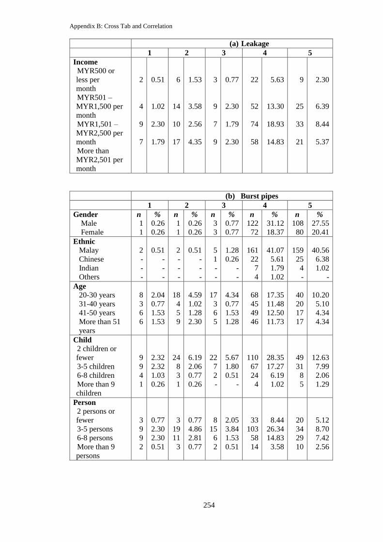
Appendix B: Cross Tab and Correlation
254
(a) Leakage
1 2 3 4 5
Income
MYR500 or
less per
month
MYR501 –
MYR1,500 per
month
MYR1,501 –
MYR2,500 per
month
More than
MYR2,501 per
month
2
4
9
7
0.51
1.02
2.30
1.79
6
14
10
17
1.53
3.58
2.56
4.35
3
9
7
9
0.77
2.30
1.79
2.30
22
52
74
58
5.63
13.30
18.93
14.83
9
25
33
21
2.30
6.39
8.44
5.37
(b) Burst pipes
1 2 3 4 5
Gender
Male
Female
n
1
1
%
0.26
0.26
n
1
1
%
0.26
0.26
n
3
3
%
0.77
0.77
n
122
72
%
31.12
18.37
n
108
80
%
27.55
20.41
Ethnic
Malay
Chinese
Indian
Others
2
-
-
-
0.51
-
-
-
2
-
-
-
0.51
-
-
-
5
1
-
-
1.28
0.26
-
-
161
22
7
4
41.07
5.61
1.79
1.02
159
25
4
-
40.56
6.38
1.02
-
Age
20-30 years
31-40 years
41-50 years
More than 51
years
8
3
6
6
2.04
0.77
1.53
1.53
18
4
5
9
4.59
1.02
1.28
2.30
17
3
6
5
4.34
0.77
1.53
1.28
68
45
49
46
17.35
11.48
12.50
11.73
40
20
17
17
10.20
5.10
4.34
4.34
Child
2 children or
fewer
3-5 children
6-8 children
More than 9
children
9
9
4
1
2.32
2.32
1.03
0.26
24
8
3
1
6.19
2.06
0.77
0.26
22
7
2
-
5.67
1.80
0.51
-
110
67
24
4
28.35
17.27
6.19
1.02
49
31
8
5
12.63
7.99
2.06
1.29
Person
2 persons or
fewer
3-5 persons
6-8 persons
More than 9
persons
3
9
9
2
0.77
2.30
2.30
0.51
3
19
11
3
0.77
4.86
2.81
0.77
8
15
6
2
2.05
3.84
1.53
0.51
33
103
58
14
8.44
26.34
14.83
3.58
20
34
29
10
5.12
8.70
7.42
2.56

Appendix B: Cross Tab and Correlation
255
(b) Burst pipes
1 2 3 4 5
House
Terraced
Two-storey
Semi-detached
Bungalow
Others
8
7
3
1
4
2.04
1.79
0.77
0.26
1.02
9
15
1
8
3
2.30
3.83
0.26
2.04
0.77
16
7
2
2
4
4.08
1.79
0.51
0.51
1.02
79
54
14
18
43
20.15
13.78
3.57
4.59
10.97
33
24
9
2
26
8.42
6.12
2.30
0.51
6.63
Education
Primary school
Secondary
College
University
degree
1
5
8
9
0.26
1.28
2.05
2.30
2
9
7
18
0.51
2.30
1.79
4.60
1
4
9
17
0.26
1.02
2.30
4.35
25
74
55
53
6.39
18.93
14.07
13.55
10
30
33
21
2.56
7.67
8.44
5.37
Work
Support staff
Professional
Others
3
12
8
0.77
3.07
2.05
8
8
20
2.05
2.05
5.12
10
8
13
2.56
2.05
3.32
62
49
97
15.86
12.53
24.81
23
29
41
5.88
7.42
10.49
Income
MYR500 or
less per
month
MYR501 –
MYR1,500 per
month
MYR1,501 –
MYR2,500 per
month
More than
MYR2,501 per
month
2
5
9
7
0.51
1.28
2.30
1.79
7
7
6
16
1.79
1.79
1.53
4.08
3
8
9
11
0.77
2.04
2.30
2.81
20
56
76
56
5.10
14.28
19.38
14.28
10
29
33
22
2.53
7.40
8.42
5.61
(c) Reservoir capacity
1 2 3 4 5
Gender
Male
Female
n
1
1
%
0.26
0.26
n
13
6
%
3.32
1.53
n
5
6
%
1.28
1.53
n
107
62
%
27.30
15.82
n
109
82
%
27.81
20.92
Ethnic
Malay
Chinese
Indian
Others
2
-
-
-
0.51
-
-
-
18
1
-
-
4.59
0.26
-
-
10
1
-
-
2.55
0.26
-
-
135
24
6
4
34.44
6.12
1.53
1.02
164
22
5
-
41.84
5.61
1.28
-
Age
20-30 years
31-40 years
41-50 years
More than 51
years
8
1
2
-
2.04
0.26
0.51
-
16
4
4
5
4.08
1.02
1.02
1.28
21
8
7
6
5.36
2.04
1.79
1.53
62
33
47
52
15.82
8.42
11.99
13.27
44
29
23
20
11.22
7.40
5.87
5.10

Appendix B: Cross Tab and Correlation
256
(c) Reservoir capacity
1 2 3 4 5
Child
2 children or
fewer
3-5 children
6-8 children
More than 9
children
8
3
-
-
2.06
0.77
-
-
19
9
-
1
4.90
2.32
-
0.26
26
10
6
-
6.70
2.58
1.55
-
102
62
23
5
26.29
15.98
5.98
1.29
59
38
12
5
15.21
9.79
3.09
1.29
Person
2 persons or
fewer
3-5 persons
6-8 persons
More than 9
persons
3
4
3
1
0.77
1.02
0.77
0.26
3
17
9
-
0.77
4.35
2.30
-
7
23
8
4
1.79
5.88
2.05
1.02
34
91
55
14
8.70
23.27
14.07
3.58
20
45
38
12
5.12
11.51
9.72
3.07
House
Terraced
Two-storey
Semi-detached
Bungalow
Others
4
1
1
1
4
1.02
0.26
0.26
0.26
1.02
13
8
3
2
3
3.32
2.04
0.77
0.51
0.77
14
9
3
10
6
3.57
2.30
0.77
2.55
1.53
77
51
14
14
38
19.64
13.01
3.57
3.57
9.69
37
38
8
4
29
9.44
9.69
2.04
1.02
7.40
Education
Primary school
Secondary
College
University
degree
2
3
1
5
0.51
0.77
0.26
1.28
-
12
5
12
-
3.07
1.28
3.07
-
5
11
26
-
1.28
2.81
6.65
28
68
50
47
7.16
17.36
12.79
12.02
9
34
45
28
2.30
8.70
11.51
7.16
Work
Support staff
Professional
Others
1
4
6
0.26
1.02
1.53
9
9
11
2.30
2.30
2.81
16
12
14
4.09
3.07
3.58
46
46
102
11.76
11.76
26.09
34
35
46
8.70
8.95
11.76
Income
MYR500 or
less per
month
MYR501 –
MYR1,500 per
month
MYR1,501 –
MYR2,500 per
month
More than
MYR2,501 per
month
2
4
2
3
0.51
1.02
0.51
0.77
3
8
4
14
0.77
2.04
1.02
3.57
4
8
11
19
1.02
2.04
2.81
4.85
23
54
66
51
5.87
13.78
16.84
13.01
10
31
50
25
2.55
7.91
12.76
6.38

Appendix B: Cross Tab and Correlation
257
(d) Water quality against Ministry of Health Standards
1 2 3 4 5
Gender
Male
Female
n
2
2
%
0.51
0.51
n
2
-
%
0.51
-
n
3
2
%
0.77
0.51
n
44
28
%
11.22
7.14
n
184
125
%
46.94
31.89
Ethnic
Malay
Chinese
Indian
Others
3
-
1
-
0.77
-
0.26
-
1
1
-
-
0.26
0.26
-
-
4
1
-
-
1.02
0.26
-
-
61
8
2
1
15.56
2.04
0.51
0.26
260
38
8
3
66.33
9.69
2.04
0.77
Age
20-30 years
31-40 years
41-50 years
More than 51
years
21
5
9
8
5.36
1.28
2.30
2.04
27
21
13
13
6.89
5.36
3.32
3.32
13
1
1
3
3.32
0.26
0.26
0.77
56
28
41
40
14.29
7.14
10.46
10.20
34
20
19
19
8.67
5.10
4.85
4.85
Child
2 children or
fewer
3-5 children
6-8 children
More than 9
children
26
14
3
-
6.70
3.61
0.77
-
39
25
7
2
10.05
6.44
1.80
0.51
13
3
1
1
3.35
0.77
0.26
0.26
88
51
20
4
22.68
13.14
5.15
1.03
48
29
10
4
12.37
7.47
2.58
1.02
Person
2 persons or
fewer
3-5 persons
6-8 persons
More than 9
persons
5
24
10
4
1.28
6.14
2.56
1.02
11
39
19
5
2.81
9.97
4.86
1.28
6
8
4
-
1.53
2.05
1.02
-
26
76
52
11
6.65
19.44
13.30
2.81
19
33
28
11
4.86
8.44
7.16
2.81
House
Terraced
Two-storey
Semi-detached
Bungalow
Others
16
11
7
4
5
4.08
2.81
1.79
1.02
1.28
29
25
2
5
13
7.40
6.38
0.51
1.28
3.32
7
2
1
5
3
1.79
0.51
0.26
1.28
0.77
63
43
13
12
34
16.07
10.97
3.32
3.06
8.67
30
26
6
5
25
7.65
6.63
1.53
1.28
6.38
Education
Primary school
Secondary
College
University
degree
3
7
12
21
0.77
1.79
3.07
5.37
4
28
19
23
1.02
7.16
12.00
21.00
-
3
6
9
-
0.77
1.53
2.30
25
53
41
45
6.39
13.35
10.49
11.51
7
31
34
20
1.79
7.93
8.70
5.12
Work
Support staff
Professional
Others
10
17
16
2.56
4.35
4.09
19
19
36
4.86
4.86
9.21
4
3
11
1.02
0.77
2.81
46
42
77
11.76
10.74
19.69
27
25
39
6.91
6.39
9.97

Appendix B: Cross Tab and Correlation
258
(d) Water quality against Ministry of Health Standards
1 2 3 4 5
Income
MYR500 or
less per
month
MYR501 –
MYR1,500 per
month
MYR1,501 –
MYR2,500 per
month
More than
MYR2,501 per
month
4
10
13
14
1.02
2.55
3.32
4.08
5
20
22
27
1.28
5.10
5.61
6.89
24
43
54
44
6.12
10.97
13.78
11.22
24
43
54
44
6.12
10.97
13.78
11.22
7
24
40
21
1.79
6.12
10.20
5.36
(e) Disruption
1 2 3 4 5
Gender
Male
Female
n
1
3
%
0.26
0.77
n
2
1
%
0.51
0.26
n
6
11
%
1.53
2.81
n
115
57
%
29.34
14.54
n
111
85
%
28.32
21.68
Ethnic
Malay
Chinese
Indian
Others
3
1
-
-
0.77
0.26
-
-
3
-
-
-
0.77
-
-
-
15
2
-
-
3.83
0.51
-
-
140
22
7
3
35.71
5.61
1.79
0.77
168
23
4
1
42.86
5.87
1.02
0.26
Age
20-30 years
31-40 years
41-50 years
More than 51
years
7
2
4
3
1.79
0.51
1.02
0.77
20
13
10
10
5.10
3.32
2.55
2.55
15
1
5
2
3.83
0.26
1.28
0.51
71
37
49
50
18.11
9.44
12.50
12.76
38
22
15
18
9.69
5.61
3.83
4.59
Child
2 children or
fewer
3-5 children
6-8 children
More than 9
children
7
6
3
-
1.80
1.55
0.77
-
33
13
4
3
8.51
3.35
1.02
0.77
17
6
-
-
4.38
1.55
-
-
108
66
25
4
27.84
17.01
6.44
1.03
49
31
9
4
12.63
7.99
2.32
1.03
Person
2 persons or
fewer
3-5 persons
6-8 persons
More than 9
persons
3
3
8
2
0.77
0.77
2.05
0.51
7
32
10
4
1.79
8.18
2.56
1.02
4
11
7
1
1.02
2.81
1.79
0.26
33
100
60
14
8.44
25.58
15.35
3.58
20
34
28
10
5.12
8.70
7.16
2.56

Appendix B: Cross Tab and Correlation
259
House
Terraced
Two-storey
Semi-detached
Bungalow
Others
5
4
3
1
3
1.28
1.02
0.77
0.26
0.77
20
17
4
7
5
5.10
4.34
1.02
1.79
1.28
12
3
1
5
2
3.06
0.77
0.26
1.28
0.51
79
58
14
16
40
20.15
14.80
3.57
4.08
10.20
29
25
7
2
30
7.40
6.38
1.79
0.51
7.65
Education
Primary school
Secondary
College
University
degree
1
3
5
7
0.26
0.77
1.28
1.79
1
16
10
26
0.26
4.09
2.56
6.65
-
4
5
14
-
1.02
1.28
3.58
26
69
56
55
6.65
17.65
14.32
14.07
11
30
36
16
2.81
7.67
9.21
4.09
Work
Support staff
Professional
Others
4
7
5
1.02
1.79
1.28
14
15
24
3.58
3.84
6.14
5
5
13
1.28
1.28
3.32
58
56
93
14.83
14.32
23.79
25
23
44
6.39
5.88
11.25
Income
MYR500 or
less per
month
MYR501 –
MYR1,500 per
month
MYR1,501 –
MYR2,500 per
month
More than
MYR2,501 per
month
2
3
5
6
0.51
0.77
1.28
1.53
5
12
10
26
1.28
3.06
2.55
6.63
3
9
6
5
0.77
2.30
1.53
1.28
24
49
77
57
6.12
12.50
19.64
14.54
8
32
35
18
2.04
8.16
8.93
4.59
(f) Connections
1 2 3 4 5
Gender
Male
Female
n
1
3
%
0.26
0.77
n
2
2
%
0.51
0.51
n
10
7
%
2.55
1.79
n
114
65
%
29.08
16.58
n
108
80
%
27.55
20.41
Ethnic
Malay
Chinese
Indian
Others
4
-
-
-
1.02
-
-
-
4
-
-
-
1.02
-
-
-
14
3
-
-
3.57
0.77
-
-
145
25
5
4
36.99
6.38
1.28
1.02
162
20
6
-
41.33
5.10
1.53
-
Age
20-30 years
31-40 years
41-50 years
More than 51
years
5
2
2
-
1.28
0.51
0.51
-
11
3
6
8
2.81
0.77
1.53
2.05
18
5
6
5
4.60
1.28
1.53
1.28
76
43
49
49
19.44
11.00
12.53
12.53
41
22
20
20
10.49
5.63
5.12
5.12

Appendix B: Cross Tab and Correlation
260
(f) Connections
1 2 3 4 5
Child
2 children or
fewer
3-5 children
6-8 children
More than 9
children
5
4
-
-
1.29
1.03
-
-
14
10
2
2
3.62
2.58
0.51
0.51
24
9
1
-
6.20
2.33
0.26
-
118
66
24
5
30.49
17.05
6.20
1.29
53
33
13
4
13.70
8.53
3.36
1.02
Person
2 persons or
fewer
3-5 persons
6-8 persons
More than 9
persons
1
4
4
-
0.26
1.02
1.02
-
3
14
9
2
0.77
3.59
2.31
0.51
7
19
5
3
1.79
4.87
1.28
0.77
35
106
62
14
8.97
27.18
15.90
3.59
21
37
32
12
5.38
9.49
8.21
3.08
House
Terraced
Two-storey
Semi-detached
Bungalow
Others
2
1
2
1
3
0.51
0.26
0.51
0.26
0.77
11
8
2
2
5
2.81
2.05
0.51
0.51
1.28
16
7
2
6
3
4.09
1.79
0.51
1.53
0.77
83
58
16
18
42
21.23
14.83
4.09
4.60
10.74
32
33
7
4
27
8.18
8.44
1.79
1.02
6.91
Education
Primary school
Secondary
College
University
degree
1
3
2
3
0.26
0.77
0.51
0.77
-
9
6
13
-
2.31
1.54
3.33
-
8
7
19
-
2.05
1.79
4.87
29
73
55
59
7.44
18.72
14.10
15.13
9
29
41
24
2.31
7.44
10.51
6.15
Work
Support staff
Professional
Others
2
3
4
0.51
0.77
1.02
5
8
15
1.28
2.05
3.85
9
12
13
2.31
3.08
3.33
64
49
104
16.41
12.56
26.67
26
33
43
6.67
8.46
11.03
Income
MYR500 or
less per
month
MYR501 –
MYR1,500 per
month
MYR1,501 –
MYR2,500 per
month
More than
MYR2,501 per
month
1
2
3
3
0.26
0.51
0.77
0.77
2
10
5
11
0.51
2.56
1.28
2.81
5
8
8
13
1.28
2.05
2.05
3.32
27
55
73
62
6.91
14.07
18.67
15.86
7
30
43
23
1.79
7.67
11.00
5.88

Appendix B: Cross Tab and Correlation
261
(g) Pressure
1 2 3 4 5
Gender
Male
Female
n
3
1
%
0.77
0.26
n
6
8
%
1.53
2.04
n
8
5
%
2.04
1.28
n
117
67
%
29.85
17.09
n
101
76
%
25.77
19.39
Ethnic
Malay
Chinese
Indian
Others
4
-
-
-
1.02
-
-
-
14
-
-
-
3.57
-
-
-
11
2
-
-
2.81
0.51
-
-
149
26
6
3
38.01
6.63
1.53
0.77
151
20
5
1
38.52
5.10
1.28
0.26
Age
20-30 years
31-40 years
41-50 years
More than 51
years
7
2
9
1
1.79
0.51
2.30
0.26
22
7
7
4
5.61
1.79
1.79
1.02
14
4
1
4
3.57
1.02
0.26
1.02
64
37
47
55
16.33
9.44
11.99
14.03
44
25
19
19
11.22
6.38
4.85
4.85
Child
2 children or
fewer
3-5 children
6-8 children
More than 9
children
10
7
1
1
2.58
1.80
0.26
0.26
24
13
3
-
6.19
3.35
0.77
-
15
6
2
-
3.87
1.55
0.51
-
106
61
26
6
27.32
15.72
6.70
1.55
59
35
9
4
15.21
9.02
2.32
1.02
Person
2 persons or
fewer
3-5 persons
6-8 persons
More than 9
persons
6
8
5
-
1.53
2.05
1.28
-
3
25
8
4
0.77
6.39
2.05
1.02
5
12
4
2
1.28
3.07
1.02
0.51
34
92
62
15
8.70
23.53
15.86
3.84
19
43
34
10
4.86
11.00
8.70
2.56
House
Terraced
Two-storey
Semi-detached
Bungalow
Others
5
5
1
3
5
1.28
1.28
0.26
0.77
1.28
18
8
4
2
8
4.59
2.04
1.02
0.51
2.04
8
4
1
4
6
2.04
1.02
0.26
1.02
1.53
80
59
14
18
32
20.41
15.05
3.57
4.59
8.16
34
31
9
4
29
8.67
7.91
2.30
1.02
7.40
Education
Primary school
Secondary
College
University
degree
1
6
4
8
0.26
1.53
1.02
2.05
2
9
10
19
0.51
2.30
2.56
4.86
-
5
7
11
-
1.28
1.79
2.81
27
67
56
52
6.91
17.14
14.32
13.35
9
35
35
28
2.30
8.95
8.95
7.16
Work
Support staff
Professional
Others
4
8
7
1.02
2.05
1.79
10
9
21
2.56
2.30
5.37
5
7
11
1.28
1.79
2.81
57
49
97
14.58
12.53
24.81
30
33
43
7.67
8.44
11.00

Appendix B: Cross Tab and Correlation
262
(g) Pressure
1 2 3 4 5
Income
MYR500 or
less per
month
MYR501 –
MYR1,500 per
month
MYR1,501 –
MYR2,500 per
month
More than
MYR2,501 per
month
3
3
8
5
0.77
0.77
2.04
1.28
7
11
6
16
1.79
2.81
1.53
4.08
3
8
5
7
0.77
2.04
1.28
1.79
22
49
73
59
5.61
12.50
18.62
15.05
7
34
41
25
1.79
8.67
10.46
6.38
(h) Price
1 2 3 4 5
Gender
Male
Female
n
41
37
%
10.46
9.44
n
94
46
%
23.98
11.73
n
26
17
%
6.63
4.34
n
41
33
%
10.46
8.42
n
33
24
%
8.42
6.12
Ethnic
Malay
Chinese
Indian
Others
63
13
2
-
16.07
3.32
0.51
-
109
22
7
2
27.81
5.61
1.79
0.51
40
2
1
-
10.20
0.51
0.26
-
67
5
-
2
17.09
1.28
-
0.51
50
6
1
-
12.76
1.53
0.26
-
Age
20-30 years
31-40 years
41-50 years
More than 51
years
15
4
13
9
3.83
1.02
3.32
2.30
24
20
19
21
6.12
5.10
4.85
5.36
13
4
3
3
3.32
1.02
0.77
0.77
67
29
35
35
17.09
7.40
8.93
8.93
32
18
13
15
8.16
4.59
3.83
3.83
Child
2 children or
fewer
3-5 children
6-8 children
More than 9
children
15
17
7
1
3.87
4.38
1.80
0.26
37
35
10
1
9.54
9.02
2.58
0.26
17
5
1
-
4.38
1.29
0.26
-
106
38
15
5
27.32
9.79
3.87
1.29
39
27
8
4
10.05
6.96
2.06
1.02
Person
2 persons or
fewer
3-5 persons
6-8 persons
More than 9
persons
4
17
14
6
1.02
4.35
3.58
1.53
9
43
26
6
2.30
11.00
6.65
1.53
7
13
2
1
1.79
3.32
0.51
0.26
33
78
45
10
8.44
19.95
11.51
2.56
14
29
26
8
3.58
7.42
6.65
2.05

Appendix B: Cross Tab and Correlation
263
(h) Price
1 2 3 4 5
House
Terraced
Two-storey
Semi-detached
Bungalow
Others
16
8
4
3
10
4.08
2.04
1.02
0.77
2.55
27
2
5
7
17
6.89
7.14
1.28
1.79
4.34
11
3
1
5
3
2.81
0.77
0.26
1.28
0.77
67
43
12
14
30
17.09
10.97
3.06
3.57
7.65
24
25
7
2
20
6.12
6.38
1.79
0.51
5.10
Education
Primary school
Secondary
College
University
degree
1
9
23
8
0.26
2.30
5.88
2.05
9
24
22
28
2.30
6.14
5.63
7.16
-
7
3
13
-
1.79
0.77
3.32
20
59
41
46
5.12
15.09
10.49
11.76
9
23
23
23
2.30
5.88
5.88
5.88
Work
Support staff
Professional
Others
13
13
15
3.32
3.32
3.84
23
24
37
5.88
6.14
9.46
8
2
13
2.05
0.51
3.32
44
40
82
11.25
10.23
20.97
18
27
32
4.60
6.91
8.18
Income
MYR500 or
less per
month
MYR501 –
MYR1,500 per
month
MYR1,501 –
MYR2,500 per
month
More than
MYR2,501 per
month
3
10
18
10
0.77
2.55
4.59
2.55
8
21
27
28
2.04
5.36
6.89
7.14
4
6
7
6
1.02
1.53
1.79
1.53
20
46
53
47
5.10
11.73
13.52
11.99
7
22
28
21
1.79
5.61
7.14
5.36

Appendix B: Cross Tab and Correlation
264
Appendix B2: Cross Tab Service Factor Improvement and Socioeconomics
(a) Reduce the level of leakage
1 2 3 4 5
Gender
Male
Female
n
2
1
%
0.51
0.26
n
4
1
%
1.02
0.26
n
6
4
%
1.56
1.02
n
110
70
%
28.6
18.2
n
113
81
%
29.38
21.06
Ethnic
Malay
Chinese
Indian
Others
3
-
-
-
0.77
-
-
-
4
1
-
-
1.02
0.26
-
-
8
2
-
-
2.08
0.51
-
-
149
20
7
4
38.01
5.10
1.79
1.02
165
25
4
-
42.09
6.38
1.02
-
Age
20-30 years
31-40 years
41-50 years
More than 51
years
-
1
1
1
-
0.26
0.26
0.26
2
1
-
2
0.51
0.26
-
0.51
5
1
2
2
1.28
0.26
0.51
0.51
56
34
45
45
14.29
8.67
11.48
11.48
88
38
35
33
22.45
9.69
8.93
8.42
Child
2 children or
fewer
3-5 children
6-8 children
More than 9
children
1
2
-
-
0.26
0.51
-
-
3
2
-
-
0.51
-
-
4
5
1
-
1.02
1.29
0.26
-
95
58
22
3
24.48
14.95
5.67
0.77
111
55
18
8
28.61
14.18
4.64
2.06
Person
2 persons or
fewer
3-5 persons
6-8 persons
More than 9
persons
-
3
-
-
-
0.77
-
-
2
2
1
-
0.51
0.51
0.26
-
-
1
7
2
-
0.26
1.79
0.51
29
85
55
11
7.42
21.74
14.07
2.81
36
89
50
18
9.21
22.76
12.79
4.60
House
Terraced
Two-storey
Semi-detached
Bungalow
Others
1
2
-
-
-
0.26
0.51
-
-
-
3
2
-
-
-
0.77
0.51
-
-
-
4
2
-
3
1
1.02
0.51
-
0.77
0.26
63
50
12
17
38
16.07
12.76
3.06
4.34
9.69
74
51
17
11
41
18.88
13.01
4.34
2.81
10.46
Education
Primary school
Secondary
College
University
Degree
1
-
2
-
0.26
-
0.26
-
-
2
1
2
-
0.51
0.26
0.51
1
2
3
4
0.26
0.51
0.77
1.02
25
61
49
44
6.39
15.60
12.53
11.25
12
57
57
68
3.07
14.58
14.58
17.39
Work
Support staff
Professional
Others
1
-
2
0.26
-
0.51
1
-
4
0.26
-
1.02
4
-
6
1.02
-
1.53
48
44
88
12.28
11.25
22.51
52
62
79
13.30
15.86
20.20

Appendix B: Cross Tab and Correlation
265
(a) Reduce the level of leakage
1 2 3 4 5
Income
MYR500 or less
per
month
MYR501 –
MYR1,500 per
month
MYR1,501 –
MYR2,500 per
month
More than
MYR2,501 per
month
-
1
2
-
-
0.26
0.51
-
2
-
1
2
0.51
-
0.26
0.51
2
5
1
2
0.51
1.28
0.26
0.51
21
46
65
48
5.36
11.73
16.58
12.24
17
53
64
60
4.34
13.52
16.58
15.31
(b) Improve repairs to burst pipes
1 2 3 4 5
Gender
Male
Female
n
1
1
%
0.26
0.26
n
1
1
%
0.26
0.26
n
3
3
%
0.51
0.51
n
122
72
%
31.72
18.72
n
108
80
%
28.08
20.8
Ethnic
Malay
Chinese
Indian
Others
2
-
-
-
0.51
-
-
-
2
-
-
-
0.51
-
-
-
5
1
-
-
1.28
0.26
-
-
161
22
7
4
41.07
5.61
1.82
1.02
159
25
4
-
40.56
6.38
1.02
-
Age
20-30 years
31-40 years
41-50 years
More than 51
years
-
-
1
1
-
-
0.26
0.26
1
1
-
-
0.26
0.26
-
-
3
1
1
1
0.77
0.26
0.26
0.26
59
35
48
52
15.05
8.93
12.24
13.27
88
38
33
29
22.45
9.69
8.42
7.40
Child
2 children or
fewer
3-5 children
6-8 children
More than 9
children
1
1
-
-
0.26
0.26
-
-
2
-
-
-
0.51
-
-
-
3
3
-
-
0.77
0.77
-
-
101
62
24
5
26.03
15.98
6.19
1.29
107
56
17
6
27.58
14.43
4.38
1.55
Person
2 persons or
fewer
3-5 persons
6-8 persons
More than 9
persons
-
2
-
-
-
0.51
-
-
-
2
-
-
-
0.51
-
-
-
2
3
1
-
0.51
0.77
0.26
29
92
59
14
7.42
23.53
15.09
3.58
38
82
51
16
9.72
20.97
13.04
4.09

Appendix B: Cross Tab and Correlation
266
(b) Improve repairs to burst pipes
1 2 3 4 5
House
Terraced
Two-storey
Semi-detached
Bungalow
Others
1
1
-
-
-
0.26
0.26
-
-
-
1
1
-
-
-
0.26
0.26
-
-
-
1
2
-
2
1
0.26
0.51
-
0.51
0.26
67
59
10
20
38
17.09
15.05
2.55
5.10
9.69
75
44
19
9
41
19.13
11.22
4.85
2.30
10.46
Education
Primary school
Secondary
College
University
degree
1
-
1
-
0.26
-
0.26
-
-
-
-
2
-
-
-
0.51
1
1
2
2
0.26
0.26
0.51
0.51
26
72
50
45
6.65
18.41
12.79
11.51
11
49
59
69
2.81
12.53
15.09
17.65
Work
Support staff
Professional
Others
-
-
2
-
-
0.26
1
-
1
0.26
-
0.26
2
-
4
0.51
-
1.02
52
47
95
13.30
12.02
24.30
51
59
77
13.04
15.09
19.69
Income
MYR500 or less
per
month
MYR501 –
MYR1,500 per
month
MYR1,501 –
MYR2,500 per
month
More than
MYR2,501 per
month
-
1
1
-
-
0.26
0.26
-
1
-
-
1
0.26
-
-
0.26
1
3
1
1
0.26
0.77
0.26
0.26
24
49
69
52
6.12
12.50
17.60
13.27
16
52
62
58
4.08
13.27
15.82
14.80
(c) Increase in reservoir capacity
1 2 3 4 5
Gender
Male
Female
n
1
1
%
0.26
0.26
n
13
6
%
3.32
1.53
n
5
6
%
1.28
1.53
n
107
62
%
27.30
15.82
n
109
82
%
27.81
20.92
Ethnic
Malay
Chinese
Indian
Others
2
-
-
-
0.51
-
-
-
18
1
-
-
4.59
0.26
-
-
10
1
-
-
2.55
0.26
-
-
135
24
6
4
34.44
6.12
1.53
1.02
164
22
5
-
41.84
5.61
1.28
-
Age
20-30 years
31-40 years
41-50 years
More than 51
years
-
-
1
1
-
-
0.26
0.26
5
3
7
4
1.28
0.77
1.79
1.02
7
2
1
1
1.79
0.51
0.26
1.26
57
30
38
44
14.54
7.65
9.69
11.22
82
40
36
33
20.92
10.20
9.18
8.42

Appendix B: Cross Tab and Correlation
267
(c) Increase in reservoir capacity
1 2 3 4 5
Child
2 children or
fewer
3-5 children
6-8 children
More than 9
children
1
1
-
-
0.26
0.26
-
-
8
7
3
1
2.06
1.08
0.77
0.26
7
3
1
-
1.80
0.77
0.26
-
94
52
18
3
24.23
13.40
4.64
0.77
104
59
19
7
26.80
15.21
4.90
1.80
Person
2 persons or
fewer
3-5 persons
6-8 persons
More than 9
persons
-
2
-
-
-
0.51
-
-
3
8
6
2
0.77
2.05
1.53
0.51
1
5
3
2
0.26
1.28
0.77
0.26
25
85
51
8
6.39
21.74
13.04
2.05
38
80
53
19
9.72
20.46
13.55
4.86
House
Terraced
Two-storey
Semi-detached
Bungalow
Others
1
1
-
-
-
0.26
0.26
-
-
-
3
6
3
4
3
0.77
1.53
0.77
1.02
0.77
3
2
1
3
2
0.77
0.51
0.26
0.77
0.51
62
52
6
16
33
15.82
13.27
1.53
4.08
8.42
76
46
19
8
42
19.39
11.73
4.85
2.04
10.71
Education
Primary school
Secondary
College
University
degree
1
-
1
-
0.26
-
0.26
-
1
7
4
7
0.26
1.78
1.02
1.78
-
3
3
5
-
0.77
0.77
1.28
23
52
45
48
5.88
13.30
11.51
12.78
14
60
59
58
3.58
15.35
15.09
14.83
Work
Support staff
Professional
Others
-
-
2
-
-
0.51
6
6
7
1.53
1.53
1.78
3
3
5
0.77
0.77
1.28
46
40
83
11.76
10.23
21.23
51
57
82
13.04
14.58
20.97
Income
MYR500 or less
per
month
MYR501 –
MYR1,500 per
month
MYR1,501 –
MYR2,500 per
month
More than
MYR2,501 per
month
-
1
1
-
-
0.26
0.26
-
2
5
4
8
0.51
1.28
1.02
2.04
2
4
3
2
0.51
1.02
0.77
0.51
19
40
66
44
4.85
14.03
15.05
11.22
19
55
59
58
4.85
10.20
16.84
14.80

Appendix B: Cross Tab and Correlation
268
(d) Improve the water quality against Ministry of Health
Standards
1 2 3 4 5
Gender
Male
Female
n
2
2
%
0.51
0.51
n
2
2
%
0.51
0.51
n
3
2
%
0.77
0.51
n
44
28
%
11.22
7.14
n
184
125
%
46.94
31.89
Ethnic
Malay
Chinese
Indian
Others
3
-
1
-
0.77
-
0.26
-
1
1
-
-
0.26
0.26
-
-
4
1
-
-
1.02
0.26
-
-
61
8
2
1
15.56
2.04
0.51
0.26
260
38
8
3
66.33
9.69
2.04
0.77
Age
20-30 years
31-40 years
41-50 years
More than 51
years
2
-
1
1
0.51
-
0.26
0.26
1
-
1
-
0.26
-
0.26
-
3
1
1
-
0.77
0.26
0.26
-
27
11
13
21
6.89
2.81
3.32
5.36
118
63
67
61
30.10
16.07
17.09
15.56
Child
2 children or
fewer
3-5 children
6-8 children
More than 9
children
3
1
-
-
0.77
0.26
-
-
1
-
1
-
0.26
-
0.26
-
2
3
-
-
0.26
0.77
-
-
38
20
12
1
9.79
5.15
3.09
0.26
170
98
28
10
43.81
25.26
7.22
2.58
Person
2 persons or
fewer
3-5 persons
6-8 persons
More than 9
persons
2
2
-
-
0.51
0.51
-
-
-
1
1
-
-
0.26
0.26
-
1
1
2
1
0.26
0.26
0.51
0.26
11
27
31
3
2.81
6.91
7.93
0.77
53
149
79
27
13.55
38.11
20.20
6.91
House
Terraced
Two-storey
Semi-detached
Bungalow
Others
3
1
-
-
-
0.77
0.26
-
-
-
-
1
-
1
-
-
0.26
-
0.26
-
1
1
-
3
-
0.26
0.26
-
0.77
-
24
15
3
9
21
6.12
3.83
0.77
2.30
5.36
117
89
26
18
59
29.85
22.70
6.63
4.59
15.05
Education
Primary school
Secondary
College
University
degree
1
1
1
1
0.26
0.26
0.26
0.26
-
-
1
1
-
-
0.26
0.26
-
1
2
2
-
0.26
0.51
0.51
17
22
15
18
4.35
5.63
3.84
4.60
21
98
93
96
5.37
25.06
2.79
24.55
Work
Support staff
Professional
Others
-
1
3
-
0.26
0.77
1
-
1
0.26
-
0.26
1
1
3
0.26
0.26
0.77
19
12
41
4.86
3.07
10.49
85
92
131
21.74
23.53
33.50

Appendix B: Cross Tab and Correlation
269
(d) Improve the water quality against Ministry of Health
Standards
1 2 3 4 5
Income
MYR500 or less
per
month
MYR501 –
MYR1,500 per
month
MYR1,501 –
MYR2,500 per
month
More than
MYR2,501 per
month
-
2
1
1
-
0.51
0.26
0.26
1
-
1
-
0.26
-
0.26
-
1
3
-
1
0.26
0.77
-
0.26
10
17
32
13
2.55
4.34
8.16
3.32
30
83
99
97
7.65
21.17
25.26
24.74
(e) Reduce water supply disruption
1 2 3 4 5
Gender
Male
Female
n
1
3
%
0.26
0.77
n
2
1
%
0.51
0.26
n
6
11
%
1.53
2.81
n
115
57
%
29.34
14.54
n
111
85
%
28.32
21.68
Ethnic
Malay
Chinese
Indian
Others
3
1
-
-
0.77
0.26
-
-
3
-
-
-
0.77
-
-
-
15
2
-
-
3.83
0.51
-
-
140
22
7
3
35.71
5.61
1.79
0.77
168
23
4
1
42.86
5.87
1.02
0.26
Age
20-30 years
31-40 years
41-50 years
More than 51
years
2
-
1
1
0.51
-
0.26
0.26
2
-
-
1
0.51
-
-
0.26
8
5
1
3
2.04
1.28
0.26
0.77
54
30
44
44
13.78
7.65
11.22
11.22
85
40
37
34
21.68
10.20
9.44
8.67
Child
2 children or
fewer
3-5 children
6-8 children
More than 9
children
3
1
-
-
0.77
0.26
-
-
3
-
-
-
0.77
-
-
-
12
3
2
-
3.09
0.77
0.51
-
87
62
18
3
22.42
15.98
4.64
0.77
109
56
21
8
28.09
14.43
5.41
2.06
Person
2 persons or
fewer
3-5 persons
6-8 persons
More than 9
persons
-
4
-
-
-
1.02
-
-
-
2
1
-
-
0.51
0.26
-
3
8
4
2
0.77
2.05
1.02
0.51
22
89
49
12
5.63
22.76
12.53
3.07
42
77
59
17
10.74
19.69
15.09
4.35
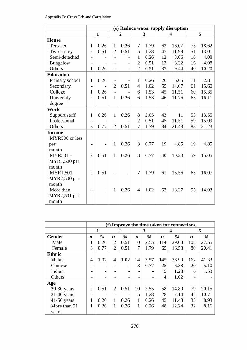
Appendix B: Cross Tab and Correlation
270
(e) Reduce water supply disruption
1 2 3 4 5
House
Terraced
Two-storey
Semi-detached
Bungalow
Others
1
2
-
-
1
0.26
0.51
-
-
0.26
1
2
-
-
-
0.26
0.51
-
-
-
7
5
1
2
2
1.79
1.28
0.26
0.51
0.51
63
47
12
13
37
16.07
11.99
3.06
3.32
9.44
73
51
16
16
40
18.62
13.01
4.08
4.08
10.20
Education
Primary school
Secondary
College
University
degree
1
-
1
2
0.26
-
0.26
0.51
-
2
-
1
-
0.51
-
0.26
1
4
6
6
0.26
1.02
1.53
1.53
26
55
45
46
6.65
14.07
11.51
11.76
11
61
60
63
2.81
15.60
15.35
16.11
Work
Support staff
Professional
Others
1
-
3
0.26
-
0.77
1
-
2
0.26
-
0.51
8
2
7
2.05
0.51
1.79
43
45
84
11
11.51
21.48
53
59
83
13.55
15.09
21.23
Income
MYR500 or less
per
month
MYR501 –
MYR1,500 per
month
MYR1,501 –
MYR2,500 per
month
More than
MYR2,501 per
month
-
2
2
-
-
0.51
0.51
-
1
1
-
1
0.26
0.26
-
0.26
3
3
7
4
0.77
0.77
1.79
1.02
19
40
61
52
4.85
10.20
15.56
13.27
19
59
63
55
4.85
15.05
16.07
14.03
(f) Improve the time taken for connections
1 2 3 4 5
Gender
Male
Female
n
1
3
%
0.26
0.77
n
2
2
%
0.51
0.51
n
10
7
%
2.55
1.79
n
114
65
%
29.08
16.58
n
108
80
%
27.55
20.41
Ethnic
Malay
Chinese
Indian
Others
4
-
-
-
1.02
-
-
-
4
-
-
-
1.02
-
-
-
14
3
-
-
3.57
0.77
-
-
145
25
5
4
36.99
6.38
1.28
1.02
162
20
6
-
41.33
5.10
1.53
-
Age
20-30 years
31-40 years
41-50 years
More than 51
years
2
-
1
1
0.51
-
0.26
0.26
2
-
1
1
0.51
-
0.26
0.26
10
5
1
1
2.55
1.28
0.26
0.26
58
28
45
48
14.80
7.14
11.48
12.24
79
42
35
32
20.15
10.71
8.93
8.16

Appendix B: Cross Tab and Correlation
271
(f) Improve the time taken for connections
1 2 3 4 5
Child
2 children or
fewer
3-5 children
6-8 children
More than 9
children
3
1
-
-
0.77
0.26
-
-
3
1
-
-
0.77
0.26
-
-
11
5
1
-
2.84
0.26
-
93
58
22
4
23.97
14.95
5.67
1.03
104
57
18
7
26.80
14.69
4.64
1.80
Person
2 persons or
fewer
3-5 persons
6-8 persons
More than 9
persons
-
4
-
-
-
1.02
-
-
-
2
2
-
-
0.51
0.51
-
4
7
4
2
1.02
1.79
1.02
0.51
27
88
53
11
6.91
22.51
13.55
2.81
36
79
54
18
9.21
20.20
13.81
4.60
House
Terraced
Two-storey
Semi-detached
Bungalow
Others
1
2
-
-
1
0.26
0.51
-
-
0.26
-
3
-
-
1
-
0.77
-
-
0.26
7
5
1
2
2
1.79
1.28
0.26
0.26
0.51
64
49
11
19
36
16.33
12.50
2.81
4.85
9.18
73
48
17
10
40
18.62
12.24
4.34
2.55
10.20
Education
Primary school
Secondary
College
University
degree
1
-
2
1
0.26
-
0.51
0.26
-
2
1
1
-
0.51
0.26
0.26
1
1
6
9
0.26
0.26
1.53
2.30
24
60
47
47
6.14
15.35
12.02
12.02
13
59
56
60
3.32
15.09
14.32
15.35
Work
Support staff
Professional
Others
1
-
3
0.26
-
0.77
2
-
2
0.51
-
0.51
8
2
7
2.05
0.51
1.79
46
45
88
11.76
11.51
22.51
49
59
79
12.33
15.09
20.20
Income
MYR500 or less
per
month
MYR501 –
MYR1,500 per
month
MYR1,501 –
MYR2,500 per
month
More than
MYR2,501 per
month
-
2
2
-
-
0.51
0.51
-
1
-
2
1
0.26
-
0.51
0.26
4
4
4
5
1.02
1.02
1.02
1.28
21
42
63
53
5.36
10.71
16.07
13.52
16
57
62
53
4.08
14.54
15.82
13.52

Appendix B: Cross Tab and Correlation
272
(g) Increase the level of pressure
1 2 3 4 5
Gender
Male
Female
n
3
1
%
0.77
0.26
n
6
8
%
1.53
2.04
n
8
5
%
2.04
1.28
n
117
67
%
29.85
17.09
n
101
76
%
25.77
19.39
Ethnic
Malay
Chinese
Indian
Others
4
-
-
-
1.02
-
-
-
14
-
-
-
3.57
-
-
-
11
2
-
-
2.81
0.51
-
-
149
26
6
3
38.01
5.10
1.28
0.77
151
20
5
1
38.52
5.10
1.28
0.26
Age
20-30 years
31-40 years
41-50 years
More than 51
years
-
2
1
1
-
0.51
0.26
0.26
8
4
-
2
2.04
1.02
-
0.51
9
2
-
2
2.30
0.51
-
0.51
54
39
42
49
13.78
9.95
10.71
12.50
80
28
40
29
20.41
7.14
10.20
7.40
Child
2 children or
fewer
3-5 children
6-8 children
More than 9
children
2
2
-
-
0.51
0.51
-
-
8
3
2
-
2.06
0.77
0.51
-
8
4
1
-
2.06
1.02
0.26
-
94
62
22
4
24.23
15.98
5.67
1.02
102
51
16
7
26.29
13.14
4.12
1.80
Person
2 persons or
fewer
3-5 persons
6-8 persons
More than 9
persons
-
4
-
-
-
-
-
-
10
3
1
-
2.55
0.77
0.26
4
3
3
3
1.02
0.77
0.77
0.77
26
92
58
8
6.63
23.53
14.83
2.05
37
71
49
19
9.46
18.16
12.54
4.86
House
Terraced
Two-storey
Semi-detached
Bungalow
Others
1
2
1
-
-
0.26
0.51
0.26
-
-
4
8
-
-
2
1.02
2.04
-
-
0.51
6
3
1
2
1
1.53
0.77
0.26
0.51
0.26
62
54
11
21
36
15.82
13.78
2.81
5.36
9.18
72
40
16
8
41
18.37
10.20
4.08
2.04
10.46
Education
Primary school
Secondary
College
University
degree
1
1
1
1
0.26
0.26
0.26
0.26
-
5
6
3
-
1.28
1.53
0.77
1
1
7
4
0.26
0.26
1.79
1.02
25
64
43
51
6.39
16.37
11.00
13.04
12
51
55
59
3.07
13.04
14.07
15.07
Work
Support staff
Professional
Others
1
-
3
0.26
-
0.77
6
1
7
1.53
0.26
1.76
4
2
7
1.02
0.51
1.79
55
43
86
14.07
11.00
21.99
41
59
76
10.49
15.09
19.44

Appendix B: Cross Tab and Correlation
273
(g) Increase the level of pressure
1 2 3 4 5
Income
MYR500 or less
per
month
MYR501 –
MYR1,500 per
month
MYR1,501 –
MYR2,500 per
month
More than
MYR2,501 per
month
-
2
1
1
-
0.51
0.26
0.26
1
4
8
1
0.26
1.02
2.04
0.26
4
4
3
2
1.02
1.02
0.77
0.51
20
42
68
54
5.10
10.71
17.35
13.78
17
53
53
54
4.34
13.52
13.52
13.78
(h) Increase in price
1 2 3 4 5
Gender
Male
Female
n
41
37
%
10.46
9.44
n
94
46
%
23.98
11.73
n
26
17
%
6.63
4.34
n
41
33
%
10.46
8.42
n
33
24
%
8.42
6.12
Ethnic
Malay
Chinese
Indian
Others
63
13
2
-
16.07
3.32
0.51
-
109
22
7
2
27.81
5.61
1.79
0.51
40
2
1
-
10.20
0.51
0.26
-
67
2
1
-
17.09
0.51
0.26
-
50
6
1
-
12.76
1.53
0.26
-
Age
20-30 years
31-40 years
41-50 years
More than 51
years
35
11
19
13
8.93
2.81
4.85
3.32
41
30
32
37
10.46
7.65
8.16
9.44
19
12
2
10
4.85
3.06
0.51
2.55
28
13
19
14
7.14
3.32
4.85
3.57
28
9
11
9
7.14
2.30
2.81
2.30
Child
2 children or
fewer
3-5 children
6-8 children
More than 9
children
43
26
7
2
11.08
6.70
1.80
0.51
70
52
13
4
18.04
13.40
3.35
1.03
28
10
3
2
7.22
2.58
0.77
0.51
40
19
11
2
10.31
4.90
2.84
0.51
33
15
7
1
8.51
3.87
1.80
0.26
Person
2 persons or
fewer
3-5 persons
6-8 persons
More than 9
persons
11
35
26
6
2.81
8.95
6.65
1.53
18
78
36
8
4.60
19.95
9.21
2.05
8
22
7
6
2.05
5.63
1.79
1.53
16
28
24
5
4.09
7.16
6.14
1.28
14
17
20
6
3.58
4.35
5.12
1.53

Appendix B: Cross Tab and Correlation
274
(h) Increase in price
1 2 3 4 5
House
Terraced
Two-storey
Semi-detached
Bungalow
Others
31
26
4
2
15
7.91
6.63
1.02
1.02
0.51
48
46
8
8
30
12.24
11.73
2.04
2.04
7.65
17
8
2
7
9
4.34
2.04
0.51
1.79
2.30
31
11
9
12
11
7.91
2.81
2.30
3.06
2.81
18
16
6
2
15
4.59
4.08
1.53
0.51
3.83
Education
Primary school
Secondary
College
University
degree
6
26
19
27
1.53
6.65
4.86
6.91
14
49
39
37
3.58
12.53
9.97
9.46
1
9
15
18
0.26
2.30
3.84
4.60
13
26
17
18
3.32
6.65
4.35
4.60
5
12
22
18
1.28
3.07
5.63
4.60
Work
Support staff
Professional
Others
16
21
20
4.09
5.37
5.12
18
16
40
4.6
4.09
10.23
19
8
16
4.86
2.05
4.09
34
40
66
8.70
10.23
16.88
19
21
37
4.86
5.37
9.46
Income
MYR500 or
less per
month
MYR501 –
MYR1,500 per
month
MYR1,501 –
MYR2,500 per
month
More than
MYR2,501 per
month
8
27
21
22
2.04
6.89
5.36
5.61
11
33
55
41
2.81
8.42
14.03
10.46
6
13
12
12
1.53
3.32
3.06
3.06
14
18
22
20
3.37
4.59
5.61
5.10
3
14
23
17
0.77
3.57
5.87
4.34

Appendix B: Cross Tab and Correlation
275
Appendix B3: Cross Tab Improvement of Strategies and Socioeconomics
(a) Setting up an integrated strategic plan
1 2 3 4 5
Gender
Male
Female
n
-
-
%
-
-
n
3
2
%
0.77
0.51
n
2
3
%
0.51
0.77
n
133
82
%
34.02
20.97
n
97
69
%
24.81
17.65
Ethnic
Malay
Chinese
Indian
Others
-
-
-
-
-
-
-
-
3
1
-
-
0.77
0.26
-
-
4
1
-
-
1.02
0.26
-
-
179
25
8
-
45.78
6.39
2.05
-
142
21
3
-
36.32
5.37
0.77
-
Age
20-30 years
31-40 years
41-50 years
More than 51
years
3
-
2
-
0.77
-
0.51
-
3
-
2
-
0.77
-
0.51
-
3
1
-
1
0.77
0.26
-
0.26
71
43
46
55
18.16
11.00
11.76
14.07
74
31
34
27
18.93
7.93
8.70
6.91
Child
2 children or
fewer
3-5 children
6-8 children
More than 9
children
-
-
-
-
-
-
-
-
3
2
-
-
0.77
0.51
-
-
3
2
-
-
0.77
0.51
-
-
114
67
26
5
29.46
17.31
6.72
1.29
94
50
15
6
24.29
12.92
3.88
1.55
Person
2 persons or
fewer
3-5 persons
6-8 persons
More than 9
persons
-
-
-
-
-
-
-
-
-
5
-
-
-
1.28
-
-
2
1
2
-
0.51
0.26
0.51
-
32
106
62
15
8.21
27.18
15.90
3.85
33
67
49
16
8.46
17.18
12.56
4.10
House
Terraced
Two-storey
Semi-detached
Bungalow
Others
-
-
-
-
-
-
-
-
-
-
2
1
2
-
-
0.51
0.26
0.51
-
-
1
1
-
1
2
0.26
0.26
-
0.26
0.51
75
67
17
20
36
19.18
17.14
4.35
5.12
9.21
67
37
10
10
42
17.14
9.46
2.56
2.56
10.74
Education
Primary school
Secondary
College
University
degree
-
-
-
-
-
-
-
-
-
-
3
2
-
-
0.77
0.51
-
2
2
1
-
0.51
0.51
0.26
25
72
51
66
6.41
18.46
13.08
16.92
14
48
55
49
3.59
12.31
14.10
12.56
Work
Support staff
Professional
Others
-
-
-
-
-
-
1
2
2
0.26
0.51
0.51
1
1
3
0.26
0.26
0.77
56
55
104
14.36
14.10
26.67
48
48
69
12.31
12.31
17.69

Appendix B: Cross Tab and Correlation
276
(a) Setting up an integrated strategic plan
1 2 3 4 5
Income
MYR500 or
less per
month
MYR501 –
MYR1,500 per
month
MYR1,501 –
MYR2,500 per
month
More than
MYR2,501 per
month
-
-
-
-
-
-
-
-
-
-
2
3
-
-
0.51
0.77
1
3
1
-
0.26
0.77
0.26
-
26
52
74
63
6.65
13.30
18.93
16.11
15
50
55
46
3.84
12.79
14.07
11.76
(b) Providing good quality training to all staff
1 2 3 4 5
Gender
Male
Female
n
-
1
%
-
0.26
n
2
1
%
0.51
0.26
n
3
3
%
0.77
0.77
n
115
63
%
29.34
16.07
n
115
89
%
29.34
16.07
Ethnic
Malay
Chinese
Indian
Others
1
-
-
1
0.26
-
-
0.26
-
2
-
1
-
0.51
-
0.26
5
1
-
-
1.28
0.26
-
-
146
22
8
2
37.24
5.61
2.04
0.51
177
23
3
1
45.15
5.87
0.77
0.26
Age
20-30 years
31-40 years
41-50 years
More than 51
years
1
-
-
-
0.26
-
-
-
2
-
1
-
0.51
-
0.26
-
1
1
3
1
0.26
0.26
0.77
0.26
56
38
38
46
14.29
9.69
9.69
11.73
91
36
41
36
23.21
9.18
10.46
9.18
Child
2 children or
fewer
3-5 children
6-8 children
More than 9
children
1
-
-
-
0.26
-
-
-
3
-
-
-
0.77
-
-
-
3
3
-
-
0.77
0.77
-
-
92
61
19
4
23.71
15.72
4.90
1.03
115
58
2
7
29.64
14.95
5.67
1.80
Person
2 persons or
fewer
3-5 persons
6-8 persons
More than 9
persons
-
-
1
-
-
-
0.26
-
-
3
-
-
-
0.77
-
-
1
2
3
-
0.26
0.51
0.77
-
30
84
52
12
7.67
21.48
13.30
3.07
36
91
57
19
9.21
23.27
14.58
4.86

Appendix B: Cross Tab and Correlation
277
(b) Providing good quality training to all staff
1 2 3 4 5
House
Terraced
Two-storey
Semi-detached
Bungalow
Others
-
-
-
-
-
-
-
-
-
-
-
2
1
-
-
-
0.51
0.26
-
-
2
1
-
1
2
0.51
0.26
-
0.26
0.51
63
54
12
21
28
16.07
13.78
3.06
5.36
7.14
80
50
16
9
49
20.41
1.76
4.08
2.30
12.50
Education
Primary school
Secondary
College
University
degree
1
-
-
-
0.26
-
-
-
-
-
1
2
-
-
0.16
0.51
-
2
4
-
-
0.56
1.02
-
24
58
40
55
6.14
14.83
10.23
14.07
14
62
67
61
3.58
15.86
17.14
15.60
Work
Support staff
Professional
Others
-
-
1
-
-
0.26
1
1
1
0.26
0.26
0.26
1
2
3
0.26
0.51
0.77
48
44
86
12.28
11.25
21.99
56
59
88
14.32
15.09
22.51
Income
MYR500 or
less per
month
MYR501 –
MYR1,500 per
month
MYR1,501 –
MYR2,500 per
month
More than
MYR2,501 per
month
-
1
-
-
-
0.26
-
-
-
1
1
2
-
0.26
0.26
0.51
1
2
2
1
0.26
0.51
0.51
0.26
22
40
62
54
5.61
10.20
15.82
13.78
19
62
68
55
4.85
15.82
17.35
14.03
(c) Increasing funding for new investment e.g.
sophisticated tools or instruments, upgrades to reservoirs
1 2 3 4 5
Gender
Male
Female
n
-
-
%
-
-
n
4
1
%
1.02
0.26
n
6
4
%
1.53
1.02
n
120
78
%
30.61
19.90
n
105
74
%
26.79
18.88
Ethnic
Malay
Chinese
Indian
Others
-
-
-
-
-
-
-
-
3
1
-
1
0.77
0.26
-
0.26
8
1
-
1
2.04
0.26
-
0.26
164
24
8
2
41.84
6.12
2.04
0.51
154
22
3
-
39.29
5.61
0.77
-

Appendix B: Cross Tab and Correlation
278
(c) Increasing funding for new investment e.g.
sophisticated tools or instruments, upgrades to reservoirs
1 2 3 4 5
Age
20-30 years
31-40 years
41-50 years
More than 51
years
-
-
-
-
-
-
-
-
1
-
2
2
0.26
-
0.51
0.51
4
2
2
2
1.02
0.51
0.51
0.51
68
37
43
50
17.35
9.44
10.97
12.76
78
36
36
29
19.90
9.18
9.18
7.40
Child
2 children or
fewer
3-5 children
6-8 children
More than 9
children
-
-
-
-
-
-
-
-
3
2
-
-
0.77
0.51
-
-
5
3
1
1
1.29
0.77
0.26
0.26
107
62
22
4
27.58
15.98
5.67
1.03
99
55
18
6
25.52
14.18
4.64
1.55
Person
2 persons or
fewer
3-5 persons
6-8 persons
More than 9
persons
-
-
-
-
-
-
-
-
-
4
1
-
-
1.02
0.26
-
1
4
4
1
0.26
1.02
1.02
0.26
33
97
54
14
8.44
24.81
13.81
3.58
33
75
54
16
8.44
19.18
13.81
4.09
House
Terraced
Two-storey
Semi-detached
Bungalow
Others
-
-
-
-
-
-
-
-
-
-
-
3
1
-
1
-
0.77
0.26
-
0.26
2
1
-
3
4
0.51
0.26
-
0.77
1.02
73
54
15
20
36
18.62
13.78
3.83
5.10
9.18
70
49
13
8
39
17.86
12.50
3.32
2.04
9.95
Education
Primary school
Secondary
College
University
degree
-
-
-
-
-
-
-
-
-
1
2
2
-
0.26
0.51
0.51
1
3
1
3
0.26
0.77
0.26
0.77
25
68
46
58
6.39
17.39
11.76
14.83
13
50
63
53
3.32
12.79
16.11
13.55
Work
Support staff
Professional
Others
-
-
-
-
-
-
1
2
2
0.26
0.51
0.51
2
1
7
0.51
0.26
1.79
48
50
100
12.28
12.79
25.58
55
53
70
14.07
13.53
17.90

Appendix B: Cross Tab and Correlation
279
(c) Increasing funding for new investment e.g.
sophisticated tools or instruments, upgrades to reservoirs
1 2 3 4 5
Income
MYR500 or
less per
month
MYR501 –
MYR1,500 per
month
MYR1,501 –
MYR2,500 per
month
More than
MYR2,501 per
month
-
-
-
-
-
-
-
-
-
2
-
3
-
0.51
-
0.77
2
2
5
1
0.51
0.51
1.28
0.26
27
51
66
54
6.89
13.01
16.84
13.78
13
50
62
54
3.32
12.76
15.82
13.78
(d) Encouraging education and awareness e.g. “Mesra
Pelanggan” (customer-friendly) roadshow
1 2 3 4 5
Gender
Male
Female
n
-
-
%
-
-
n
3
2
%
0.77
0.51
n
6
3
%
1.53
0.77
n
109
67
%
27.81
17.09
n
117
85
%
29.85
21.68
Ethnic
Malay
Chinese
Indian
Others
-
-
-
-
-
-
-
-
3
1
-
1
0.77
0.26
-
0.26
8
1
-
-
2.04
0.26
-
-
144
23
7
2
36.73
5.87
1.79
0.51
174
23
4
1
44.39
5.87
1.02
0.26
Age
20-30 years
31-40 years
41-50 years
More than 51
years
-
-
-
-
-
-
-
-
2
-
1
2
0.51
-
0.26
0.51
4
2
1
2
1.02
0.51
0.26
0.51
57
33
41
45
14.54
8.42
10.46
11.48
88
40
40
34
22.45
10.20
10.20
8.67
Child
2 children or
fewer
3-5 children
6-8 children
More than 9
children
-
-
-
-
-
-
-
-
5
-
-
-
1.29
-
-
-
4
4
-
1
1.03
1.03
-
0.26
89
59
22
4
22.94
15.21
5.67
1.03
116
59
19
6
29.90
15.21
4.90
1.55
Person
2 persons or
fewer
3-5 persons
6-8 persons
More than 9
persons
-
-
-
-
-
-
-
-
1
4
-
-
0.26
1.02
-
-
1
5
3
-
0.26
1.28
0.77
-
26
87
50
13
6.65
22.25
12.79
3.32
39
84
60
18
9.97
21.48
15.35
4.60

Appendix B: Cross Tab and Correlation
280
(d) Encouraging education and awareness e.g. “Mesra
Pelanggan” (customer-friendly) roadshow
1 2 3 4 5
House
Terraced
Two-storey
Semi-detached
Bungalow
Others
-
-
-
-
-
-
-
-
-
-
1
3
1
-
-
0.26
0.77
0.26
-
-
1
1
-
4
3
0.26
0.26
-
1.02
0.77
65
55
11
16
29
16.58
14.03
2.81
4.08
7.40
78
48
17
11
48
19.90
12.24
4.34
2.81
12.24
Education
Primary school
Secondary
College
University
degree
-
-
-
-
-
-
-
-
-
-
2
3
-
-
0.51
0.77
-
2
2
5
-
0.51
0.51
1.28
21
58
45
51
5.37
14.83
11.51
13.04
18
62
63
59
4.60
15.86
16.11
15.09
Work
Support staff
Professional
Others
-
-
-
-
-
-
-
3
2
-
0.77
0.51
3
1
5
0.77
0.26
1.28
44
46
86
11.25
11.76
21.99
59
56
86
15.09
14.32
21.99
Income
MYR500 or
less per
month
MYR501 –
MYR1,500 per
month
MYR1,501 –
MYR2,500 per
month
More than
MYR2,501 per
month
-
-
-
-
-
-
-
-
-
1
1
3
-
0.26
0.26
0.77
2
3
3
1
0.51
0.77
0.77
0.26
22
41
62
51
5.61
10.46
15.82
13.01
18
60
67
57
4.59
15.31
17.09
14.54

Appendix B: Cross Tab and Correlation
281
Appendix B4
Appendix B4.1 (a): Correlation of Service Quality Performance with Malay
Spearman Correlation Coefficients, n = 329
Prob > |r| under H0: Rho=0
Leakage Burst Pipes Reservoir Water Quality Disruption Connection Pressure Price
Leakage 1.00000 0.81343
(<.0001)*
0.50859
(<.0001)*
0.45047
(<.0001)*
0.64890
(<.0001)*
0.54019
(<.0001)*
0.52930
(<.0001)*
0.26410
(<.0001)*
Burst Pipes 0.81343
(<.0001)*
1.00000 0.53834
(<.0001)*
0.46955
(<.0001)*
0.68564
(<.0001)*
0.58344
(<.0001)*
0.54467
(<.0001)*
0.21771
(<.0001)*
Reservoir 0.50859
(<.0001)*
0.53834
(<.0001)*
1.00000 0.42760
(<.0001)*
0.61447
(<.0001)*
0.58685
(<.0001)*
0.58342
(<.0001)*
0.22223
(<.0001)*
Water
Quality
0.45047
(<.0001)*
0.46955
(<.0001)*
0.42760
(<.0001)*
1.00000 0.53652
(<.0001)*
0.46456
(<.0001)*
0.39188
(<.0001)*
0.21771
(<.0001)*
Disruption 0.64890
(<.0001)*
0.68564
(<.0001)*
0.61447
(<.0001)*
0.53652
(<.0001)*
1.00000
0.66299
(<.0001)*
0.58593
(<.0001)*
0.26232
(<.0001)*
Connection 0.54019
(<.0001)*
0.58344
(<.0001)*
0.58685
(<.0001)*
0.46456
(<.0001)*
0.66299
(<.0001)*
1.00000 0.64974
(<.0001)*
0.27382
(<.0001)*
Pressure 0.52930
(<.0001)*
0.54467
(<.0001)*
0.58342
(<.0001)*
0.39188
(<.0001)*
0.58593
(<.0001)*
0.64974
(<.0001)*
1.00000
0.27349
(<.0001)*
Price 0.26410
(<.0001)*
0.21771
(<.0001)*
0.22223
(<.0001)*
0.21771
(<.0001)*
0.26232
(<.0001)*
0.27382
(<.0001)*
0.27349
(<.0001)*
1.00000
* Significant at 1%

Appendix B: Cross Tab and Correlation
282
Appendix B4.1 (b): Correlation of Service Quality Performance with Chinese
Spearman Correlation Coefficients, n = 48
Prob > |r| under H0: Rho=0
Leakage Burst Pipes Reservoir Water Quality Disruption Connection Pressure Price
Leakage 1.00000
0.93423
(<.0001)*
0.79404
(<.0001)*
0.57247
(<.0001)*
0.73342
(<.0001)*
0.73246
(<.0001)*
0.61692
(<.0001)*
0.73078
(<.0001)*
Burst Pipes 0.93423
(<.0001)*
1.00000
0.81862
(<.0001)*
0.64037
(<.0001)*
0.75073
(<.0001)*
0.67850
(<.0001)*
0.57615
(<.0001)*
0.77010
(<.0001)*
Reservoir 0.79404
(<.0001)*
0.81862
(<.0001)*
1.00000
0.79555
(<.0001)*
0.89704
(<.0001)*
0.82564
(<.0001)*
0.67033
(<.0001)*
0.60980
(<.0001)*
Water
Quality
0.57247
(<.0001)*
0.64037
(<.0001)*
0.79555
(<.0001)*
1.00000
0.67748
(<.0001)*
0.58727
(<.0001)*
0.63481
(<.0001)*
0.56845
(<.0001)*
Disruption 0.73342
(<.0001)*
0.75073
(<.0001)*
0.89704
(<.0001)*
0.67748
(<.0001)*
1.00000
0.79042
(<.0001)*
0.58940
(<.0001)*
0.59532
(<.0001)*
Connection 0.73246
(<.0001)*
0.67850
(<.0001)*
0.82564
(<.0001)*
0.58727
(<.0001)*
0.79042
(<.0001)*
1.00000
0.72393
(<.0001)*
0.48633
(<.0005)*
Pressure 0.61692
(<.0001)*
0.57615
(<.0001)*
0.67033
(<.0001)*
0.63481
(<.0001)*
0.58940
(<.0001)*
0.72393
(<.0001)*
1.00000
0.57573
(<.0001)*
Price 0.73078
(<.0001)*
0.77010
(<.0001)*
0.60980
(<.0001)*
0.56845
(<.0001)*
0.59532
(<.0001)*
0.48633
(<.0005)*
0.57573
(<.0001)*
1.00000
* Significant at 1%

Appendix B: Cross Tab and Correlation
283
Appendix B4.1 (c): Correlation of Service Quality Performance with Indian
Spearman Correlation Coefficients, n = 11
Prob > |r| under H0: Rho=0
Leakage Burst Pipes Reservoir Water Quality Disruption Connection Pressure Price
Leakage 1.00000
0.90830
(0.0001)*
0.90830
(0.0001)*
0.73068
(0.0106)**
0.49054
0.1255
0.72866
(0.0110)**
0.69921
(0.0166)**
0.13587
0.6904
Burst Pipes 0.90830
(0.0001)*
1.00000
1.00000
(<.0001)*
0.85635
(0.0008)*
0.81009
(0.0025)*
0.85398
(0.0008)*
0.75993
(0.0066)*
0.27425
0.4144
Reservoir 0.90830
(0.0001)*
1.00000
(<.0001)*
1.00000
0.85635
(0.0008)*
0.81009
(0.0025)*
0.85398
(0.0008)*
0.75993
(0.0066)*
0.27425
0.4144
Water
Quality
0.73068
(0.0106)**
0.85635
(0.0008)*
0.85635
(0.0008)*
1.00000
0.75979
(0.0067)*
0.64266
(0.0330)**
0.44230
0.1731
0.02135
0.9503
Disruption 0.49054
0.1255
0.68564
(0.0025)*
0.81009
(0.0025)*
0.75979
(0.0067)*
1.00000
0.75769
(0.0069)*
0.60305
(0.0495)**
0.38086
0.2478
Connection 0.72866
(0.0110)**
0.85398
(0.0008)*
0.85398
(0.0008)*
0.64266
(0.0330)**
0.75769
(0.0069)*
1.00000
0.80348
(0.0029)*
0.36195
0.2740
Pressure 0.69921
(0.0166)**
0.75993
(0.0066)*
0.75993
(0.0066)*
0.44230
0.1731
0.60305
(0.0495)**
0.80348
(0.0029)*
1.00000
0.40059
0.2221
Price 0.13587
0.6904
0.27425
0.4144
0.27425
0.4144
0.02135
0.9503
0.38086
0.2478
0.36195
0.2740
0.40059
0.2221
1.00000
* Significant at 1% ** Significant at 1%

Appendix B: Cross Tab and Correlation
284
Appendix B4.2 (a): Correlation of Service Quality Performance with Age (20 to 30 years old)
Pearson Correlation Coefficients, n = 151
Prob > |r| under H0: Rho=0
Leakage Burst Pipes Reservoir Water Quality Disruption Connection Pressure Price
Leakage 1.00000
0.81835
(<.0001)*
0.51118
(<.0001)*
0.43307
(<.0001)*
0.62176
(<.0001)*
0.51702
(<.0001)*
0.45909
(<.0001)*
0.25536
(0.0016)*
Burst Pipes 0.81835
(<.0001)*
1.00000
0.55436
(<.0001)*
0.50838
(<.0001)*
0.70144
(<.0001)*
0.52783
(<.0001)*
0.45032
(<.0001)*
0.28842
(0.0003)*
Reservoir 0.51118
(<.0001)*
0.55436
(<.0001)*
1.00000
0.47410
(<.0001)*
0.67707
(<.0001)*
0.43853
(<.0001)*
0.45286
(<.0001)*
0.27293
(0.0007)*
Water
Quality
0.43307
(<.0001)*
0.50838
(<.0001)*
0.47410
(<.0001)*
1.00000
0.58707
(<.0001)*
0.45203
(<.0001)*
0.39740
(<.0001)*
0.28010
(0.0005)*
Disruption 0.62176
(<.0001)*
0.70144
(<.0001)*
0.67707
(<.0001)*
0.58707
(<.0001)*
1.00000
0.54708
(<.0001)*
0.56422
(<.0001)*
0.29032
(0.0003)*
Connection 0.51702
(<.0001)*
0.52783
(<.0001)*
0.43853
(<.0001)*
0.45203
(<.0001)*
0.54708
(<.0001)*
1.00000
0.54031
(<.0001)*
0.18737
(0.0212)**
Pressure 0.45909
(<.0001)*
0.45032
(<.0001)*
0.45286
(<.0001)*
0.39740
(<.0001)*
0.56422
(<.0001)*
0.54031
(<.0001)*
1.00000
0.21347
(0.0085)*
Price 0.25536
(0.0016)*
0.28842
(0.0003)*
0.27293
(0.0007)*
0.28010
(0.0005)*
0.29032
(0.0003)*
0.18737
(0.0212)**
0.21347
(0.0085)*
1.00000
* Significant at 1% ** Significant at 5%

Appendix B: Cross Tab and Correlation
285
Appendix B4.2 (b): Correlation of Service Quality Performance with Age (31 to 40 years old)
Pearson Correlation Coefficients, n = 75
Prob > |r| under H0: Rho=0
Leakage Burst Pipes Reservoir Water Quality Disruption Connection Pressure Price
Leakage 1.00000
0.91955
(<.0001)*
0.68685
(<.0001)*
0.51086
(<.0001)*
0.82633
(<.0001)*
0.77150
(<.0001)*
0.64061
(<.0001)*
0.32596
(0.0043)*
Burst Pipes 0.91955
(<.0001)*
1.00000
0.69535
(<.0001)*
0.46289
(<.0001)*
0.82407
(<.0001)*
0.81759
(<.0001)*
0.68230
(<.0001)*
0.31628
(0.0057)*
Reservoir 0.68685
(<.0001)*
0.69535
(<.0001)*
1.00000
0.55093
(<.0001)*
0.65092
(<.0001)*
0.75612
(<.0001)*
0.63555
(<.0001)*
0.30711
(0.0074)*
Water
Quality
0.51086
(<.0001)*
0.46289
(<.0001)*
0.55093
(<.0001)*
1.00000
0.52536
(<.0001)*
0.52899
(<.0001)*
0.52018
(<.0001)*
0.45542
(<.0001)*
Disruption 0.82633
(<.0001)*
0.82407
(<.0001)*
0.65092
(<.0001)*
0.52536
(<.0001)*
1.00000
0.77448
(<.0001)*
0.65409
(<.0001)*
0.28248
(0.0141)**
Connection 0.77150
(<.0001)*
0.81759
(<.0001)*
0.75612
(<.0001)*
0.52899
(<.0001)*
0.77448
(<.0001)*
1.00000
0.67397
(<.0001)*
0.40879
(0.0003)*
Pressure 0.64061
(<.0001)*
0.68230
(<.0001)*
0.63555
(<.0001)*
0.52018
(<.0001)*
0.65409
(<.0001)*
0.67397
(<.0001)*
1.00000
0.28090
(0.0146)**
Price 0.32596
(0.0043)*
0.31628
(0.0057)*
0.30711
(0.0074)*
0.45542
(<.0001)*
0.28248
(0.0141)**
0.40879
(0.0003)*
0.28090
(0.0146)**
1.00000
* Significant at 1% ** Significant at 5%

Appendix B: Cross Tab and Correlation
286
Appendix B4.2 (c): Correlation of Service Quality Performance and Age (41 to 50 years old)
Pearson Correlation Coefficients, n = 83
Prob > |r| under H0: Rho=0
Leakage Burst Pipes Reservoir Water Quality Disruption Connection Pressure Price
Leakage 1.00000
0.92907
(<.0001)*
0.56533
(<.0001)*
0.36268
0.0008
0.52287
(<.0001)*
0.57453
(<.0001)*
0.40082
(0.0002)*
0.09563
0.3898
Burst Pipes 0.92907
<.0001*
1.00000
0.58718
(<.0001)*
0.35911
0.0009
0.51721
(<.0001)*
0.54226
(<.0001)*
0.39490
0.0002
0.04384
0.6939
Reservoir 0.56533
(<.0001)*
0.58718
(<.0001)*
1.00000
0.46629
(<.0001)*
0.71810
(<.0001)*
0.73038
(<.0001)*
0.61604
(<.0001)*
0.12673
0.2536
Water
Quality
0.36268
(0.0008)*
0.35911
(0.0009)*
0.46629
(<.0001)*
1.00000
0.60658
(<.0001)*
0.49901
(<.0001)*
0.37098
(0.0006)*
0.08710
0.4336
Disruption 0.52287
(<.0001)*
0.51721
(<.0001)*
0.71810
(<.0001)*
0.60658
(<.0001)*
1.00000
0.70262
(<.0001)*
0.39850
(0.0002)*
0.10357
0.3515
Connection 0.57453
(<.0001)*
0.54226
(<.0001)*
0.73038
(<.0001)*
0.49901
(<.0001)*
0.70262
(<.0001)*
1.00000
0.56907
(<.0001)*
0.17339
0.1170
Pressure 0.40082
(0.0002)*
0.39490
(0.0002)*
0.61604
(<.0001)*
0.37098
(0.0006)*
0.39850
(0.0002)*
0.56907
(<.0001)*
1.00000
0.15551
0.1604
Price 0.09563
0.3898
0.04384
0.6939
0.12673
0.2536
0.08710
0.4336
0.10357
0.3515
0.17339
0.1170
0.15551
0.1604
1.00000
* Significant at 1% ** Significant at 5%

Appendix B: Cross Tab and Correlation
287
Appendix B4.2 (d): Correlation of Service Quality Performance and Age (More than 51 years old)
Pearson Correlation Coefficients, n = 83
Prob > |r| under H0: Rho=0
Leakage Burst Pipes Reservoir Water Quality Disruption Connection Pressure Price
Leakage 1.00000
0.69390
(<.0001)*
0.11966
0.2813
0.33598
(0.0019)*
0.45699
(<.0001)*
0.18496
0.0962
0.31581
(0.0036)*
0.41843
(<.0001)*
Burst Pipes 0.69390
(<.0001)*
1.00000
0.20407
0.0642
0.37496
(0.0005)*
0.48943
(<.0001)*
0.27812
(0.0114)**
0.31264
(0.0040)*
0.24011
(0.0288)**
Reservoir 0.11966
0.2813
0.20407
0.0642
1.00000
0.18820
0.0884
0.34666
(0.0013)*
0.55432
(<.0001)*
0.31642
(0.0036)*
0.10775
0.3322
Water
Quality
0.33598
(0.0019)*
0.37496
(0.0005)*
0.18820
0.0884
1.00000
0.25181
(0.0216)**
0.22039
(0.0466)**
0.09613
0.3873
0.10629
0.3389
Disruption 0.45699
(<.0001)*
0.48943
(<.0001)*
0.34666
(0.0013)*
0.25181
(0.0216)**
1.00000
0.58774
(<.0001)*
0.44916
(<.0001)*
0.29010
(0.0078)*
Connection 0.18496
0.0962
0.27812
(0.0114)**
0.55432
(<.0001)*
0.22039
(0.0466)**
0.58774
(<.0001)*
1.00000
0.52459
(<.0001)*
0.19256
0.0831
Pressure 0.31581
(0.0036)*
0.31264
(0.0040)*
0.31642
(0.0036)*
0.09613
0.3873
0.44916
(<.0001)*
0.52459
(<.0001)*
1.00000
0.41899
(<.0001)*
Price 0.41843
(<.0001)*
0.24011
(0.0288)**
0.10775
0.3322
0.10629
0.3389
0.29010
(0.0078)*
0.19256
0.0831
0.41899
(<.0001)*
1.00000
* Significant at 1% ** Significant at 5%

Appendix B: Cross Tab and Correlation
288
Appendix B4.3 (a): Correlation of Service Quality Performance with Child (2 children and fewer)
Pearson Correlation Coefficients, n = 214
Prob > |r| under H0: Rho=0
Leakage Burst Pipes Reservoir Water Quality Disruption Connection Pressure Price
Leakage 1.00000 0.81176
(<.0001)*
0.51545
(<.0001)*
0.41150
(<.0001)*
0.63063
(<.0001)*
0.49800
(<.0001)*
0.44746
(<.0001)*
0.17086
(0.0123)**
Burst Pipes 0.81176
(<.0001)*
1.00000 0.57695
(<.0001)*
0.45096
(<.0001)*
0.68869
(<.0001)*
0.50184
(<.0001)*
0.42876
(<.0001)*
0.20503
(0.0026)*
Reservoir 0.51545
(<.0001)*
0.57695
(<.0001)*
1.00000 0.46144
(<.0001)*
0.62046
(<.0001)*
0.47219
(<.0001)*
0.50681
(<.0001)*
0.24178
(0.0004)*
Water
Quality
0.41150
(<.0001)*
0.45096
(<.0001)*
0.46144
(<.0001)*
1.00000 0.49428
(<.0001)*
0.37683
(<.0001)*
0.37096
(<.0001)*
0.20286
(0.0029)*
Disruption 0.63063
(<.0001)*
0.68869
(<.0001)*
0.62046
(<.0001)*
0.49428
(<.0001)*
1.00000 0.54238
(<.0001)*
0.57144
(0.0046)*
0.19294
(0.0046)*
Connection 0.49800
(<.0001)*
0.50184
(<.0001)*
0.47219
(<.0001)*
0.37683
(<.0001)*
0.54238
(<.0001)*
1.00000 0.53584
(<.0001)*
0.17786
(0.0091)*
Pressure 0.44746
(<.0001)*
0.42876
(<.0001)*
0.50681
(<.0001)*
0.37096
(<.0001)*
0.57144
(<.0001)*
0.53584
(<.0001)*
1.00000 0.16999
(0.0128)**
Price 0.17086
(0.0123)**
0.20503
(0.0026)*
0.24178
(0.0004)*
0.20286
(0.0029)*
0.19294
(0.0046)*
0.17786
(0.0091)*
0.16999
(0.0128)**
1.00000
* Significant at 1% ** Significant at 5%

Appendix B: Cross Tab and Correlation
289
Appendix B4.3 (b): Correlation of Service Quality Performance with Child (3–5 children)
Pearson Correlation Coefficients, n = 122
Prob > |r| under H0: Rho=0
Leakage Burst Pipes Reservoir Water Quality Disruption Connection Pressure Price
Leakage 1.00000 0.86988
(<.0001)*
0.54983
(<.0001)*
0.38497
(<.0001)*
0.56894
(<.0001)*
0.61403
(<.0001)*
0.49089
(<.0001)*
0.37112
(<.0001)*
Burst Pipes 0.86988
(<.0001)*
1.00000 0.52390
(<.0001)*
0.36780
(<.0001)*
0.60451
(<.0001)*
0.58960
(<.0001)*
0.47254
(<.0001)*
0.27629
(0.0021)*
Reservoir 0.54983
(<.0001)*
0.52390
(<.0001)*
1.00000 0.42999
(<.0001)*
0.74720
(<.0001)*
0.73621
(<.0001)*
0.55302
(<.0001)*
0.21125
(0.0195)**
Water
Quality
0.38497
(<.0001)*
0.36780
(<.0001)*
0.42999
(<.0001)*
1.00000 0.55386
(<.0001)*
0.51159
(<.0001)*
0.41847
(0.0062)*
0.24631
(0.0062)*
Disruption 0.56894
(<.0001)*
0.60451
(<.0001)*
0.74720
(<.0001)*
0.55386
(<.0001)*
1.00000 0.78553
(<.0001)*
0.51997
(0.0029)*
0.26786
(0.0029)*
Connection 0.61403
(<.0001)*
0.58960
(<.0001)*
0.73621
(<.0001)*
0.51159
(<.0001)*
0.78553
(<.0001)*
1.00000 0.63196
(<.0001)*
0.28613
(0.0014)*
Pressure 0.49089
(<.0001)*
0.47254
(<.0001)*
0.55302
(<.0001)*
0.41847
(<.0001)*
0.51997
(<.0001)*
0.63196
(<.0001)*
1.00000 0.28082
(0.0017)*
Price 0.37112
(<.0001)*
0.27629
(0.0021)*
0.21125
(0.0195)**
0.24631
(0.0062)*
0.26786
(0.0029)*
0.28613
(0.0014)*
0.28082
(0.0017)*
1.00000
* Significant at 1% ** Significant at 5%

Appendix B: Cross Tab and Correlation
290
Appendix B4.3 (c): Correlation of Service Quality Performance with Child (68 children)
Pearson Correlation Coefficients, n = 41
Prob > |r| under H0: Rho=0
Leakage Burst Pipes Reservoir Water Quality Disruption Connection Pressure Price
Leakage 1.00000
0.78990
(<.0001)*
0.23111
0.1460
0.46360
(0.0023)*
0.54156
(0.0003)*
0.20649
0.2011
0.19744
0.2160
0.31208
(0.0470)**
Burst Pipes 0.78990
(<.0001)*
1.00000
0.2380
0.18845
(0.0002)*
0.55237
(0.0048)*
0.43221
(0.0466)**
0.31658
0.0587
0.29776
0.4039
0.13391
0.4039
Reservoir 0.23111
0.1460
0.18845
0.2380
1.00000
0.27949
0.0768
0.20998
0.1876
0.54713
(0.0003)*
0.39761
(0.0100)*
0.23695
0.1358
Water
Quality
0.46360
(0.0023)*
0.55237
(0.0002)*
0.27949
0.0768
1.00000
0.41873
(0.0064)*
0.36766
(0.0196)**
0.05243
0.7448
0.20090
0.2078
Disruption 0.54156
(0.0003)*
0.43221
(0.0048)*
0.20998
0.1876
0.41873
(0.0064)*
1.00000
0.47617
(0.0019)*
0.16477
0.3032
0.35939
(0.0210)**
Connection 0.20649
0.2011 0.31658
(0.0466)**
0.54713
(0.0003)*
0.36766
(0.0196)**
0.47617
(0.0019)*
1.00000
0.32621
(0.0400)**
0.15610
0.3361
Pressure 0.19744
0.2160
0.29776
0.0587
0.39761
(0.0100)*
0.05243
0.7448
0.16477
0.3032
0.32621
(0.0400)**
1.00000
0.31604
(0.0441)**
Price 0.31208
(0.0470)**
0.13391
0.4039
0.23695
0.1358
0.20090
0.2078
0.35939
(0.0210)**
0.15610
0.3361
0.31604
(0.0441)**
1.00000
* Significant at 1% ** Significant at 5%

Appendix B: Cross Tab and Correlation
291
Appendix B4.3 (d): Correlation of Service Quality Performance with Child (More than 9 children)
Pearson Correlation Coefficients, n = 11
Prob > |r| under H0: Rho=0
Leakage Burst Pipes Reservoir Water Quality Disruption Connection Pressure Price
Leakage 1.00000 0.89360
(0.0002)*
0.04303
0.9000
0.54130
0.0855 0.70973
(0.0144)*
0.78174
(0.0045)*
0.96612
(<.0001)*
0.86809
(0.0005)*
Burst Pipes 0.89360
(0.0002)*
1.00000 0.41201
0.2080 0.72162
(0.0122)**
0.83450
(0.0014)*
0.95258
(<.0001)*
0.85282
(0.0008)*
0.74516
(0.0085)*
Reservoir
0.04303
0.9000
0.41201
0.2080
1.00000 0.70766
(0.0148)**
0.57869
0.0622 0.60553
(0.0484)**
0.07077
0.8362
0.10821
0.7515
Water
Quality
0.54130
0.0855 0.72162
(0.0122)**
0.70766
(0.0148)**
1.00000 0.97260
(<.0001)*
0.80345
(0.0029)*
0.54930
0.0801 0.73838
(0.0095)*
Disruption 0.70973
(0.0144)**
0.83450
(0.0014)**
0.57869
0.0622 0.97260
(<.0001)*
1.00000 0.87604
(0.0004)*
0.71665
(0.0131)**
0.84981
(0.0009)*
Connection 0.78174
(0.0045)*
0.95258
(<.0001)*
0.60553
(0.0484)**
0.80345
(0.0029)*
0.87604
(0.0004)*
1.00000 0.80345
(0.0029)*
0.70202
(0.0160)**
Pressure 0.96612
(<.0001)*
0.85282
(0.0008)*
0.07077
0.8362
0.54930
0.0801 0.71665
(0.0131)**
0.80345
(0.0029)**
1.00000 0.88606
(0.0003)*
Price 0.86809
(0.0005)*
0.74516
(0.0085)*
0.10821
0.7515 0.73838
(0.0095)*
0.84981
(0.0009)*
0.70202
(0.0160)**
0.88606
(0.0003)*
1.00000
* Significant at 1% ** Significant at 5%

Appendix B: Cross Tab and Correlation
292
Appendix B4.4 (a): Correlation of Service Quality Performance with Person (2 persons or fewer)
Pearson Correlation Coefficients, n = 67
Prob > |r| under H0: Rho=0
Leakage Burst Pipes Reservoir Water Quality Disruption Connection Pressure Price
Leakage 1.00000 0.85976
(<.0001)*
0.59235
(<.0001)*
0.45241
(0.0001)*
0.74065
(<.0001)*
0.82738
(<.0001)*
0.54059
(<.0001)*
0.27614
(0.0237)**
Burst Pipes 0.85976
(<.0001)*
1.00000 0.55587
(<.0001)*
0.47558
(<.0001)*
0.67300
(<.0001)*
0.79310
(<.0001)*
0.43614
(0.0002)**
0.29124
(0.0168)**
Reservoir 0.59235
(<.0001)*
0.55587
(<.0001)*
1.00000 0.50719
(<.0001)*
0.72092
(<.0001)*
0.60307
(<.0001)*
0.48042
(<.0001)*
0.04423
0.7223
Water
Quality
0.45241
(0.0001)*
0.47558
(<.0001)*
0.50719
(<.0001)*
1.00000 0.53389
(<.0001)*
0.49993
(<.0001)*
0.57376
(<.0001)*
0.24032
(0.0501)**
Disruption 0.74065
(<.0001)*
0.67300
(<.0001)*
0.72092
(<.0001)*
0.53389
(<.0001)*
1.00000 0.70547
(<.0001)*
0.64826
(<.0001)*
0.30138
(0.0132)**
Connection 0.82738
(<.0001)*
0.79310
(<.0001)*
0.60307
(<.0001)*
0.49993
(<.0001)*
0.70547
(<.0001)*
1.00000 0.52964
(<.0001)*
0.33758
(0.0052)*
Pressure 0.54059
(<.0001)*
0.43614
(0.0002)**
0.48042
(<.0001)*
0.57376
(<.0001)*
0.64826
(<.0001)*
0.52964
(<.0001)*
1.00000 0.19089
0.1218
Price 0.27614
(0.0237)**
0.29124
(0.0168)**
0.04423
0.7223
0.24032
0.0501 0.30138
(0.0132)**
0.33758
(0.0052)*
0.19089
0.1218
1.00000
* Significant at 1% ** Significant at 5%

Appendix B: Cross Tab and Correlation
293
Appendix B4.4 (b): Correlation of Service Quality Performance with Person (3 to 5 persons)
Pearson Correlation Coefficients, n = 180
Prob > |r| under H0: Rho=0
Leakage Burst Pipes Reservoir Water Quality Disruption Connection Pressure Price
Leakage 1.00000
0.78785
(<.0001)*
0.38717
(<.0001)*
0.34748
(<.0001)*
0.52209
(<.0001)*
0.39796
(<.0001)*
0.37946
(<.0001)*
0.29684
(<.0001)*
Burst Pipes 0.78785
(<.0001)*
1.00000
0.40793
(<.0001)*
0.36571
(<.0001)*
0.57445
(<.0001)*
0.37724
(<.0001)*
0.36559
(<.0001)*
0.23382
(0.0016)*
Reservoir 0.38717
(<.0001)*
0.40793
(<.0001)*
1.00000
0.34661
(<.0001)*
0.57172
(<.0001)*
0.52400
(<.0001)*
0.47717
(<.0001)*
0.29540
(<.0001)*
Water
Quality
0.34748
(<.0001)*
0.36571
(<.0001)*
0.34661
(<.0001)*
1.00000
0.40699
(<.0001)*
0.31106
(<.0001)*
0.24499
(0.0009)*
0.22595
(0.0023)*
Disruption 0.52209
(<.0001)*
0.57445
(<.0001)*
0.57172
(<.0001)*
0.40699
(<.0001)*
1.00000
0.60133
(<.0001)*
0.52309
(<.0001)*
0.23155
(0.0018)*
Connection 0.39796
(<.0001)*
0.37724
(<.0001)*
0.52400
(<.0001)*
0.31106
(<.0001)*
0.60133
(<.0001)*
1.00000
0.50007
(<.0001)*
0.23172
(0.0017)*
Pressure 0.37946
(<.0001)*
0.36559
(<.0001)*
0.47717
(<.0001)*
0.24499
(0.0009)*
0.52309
(<.0001)*
0.50007
(<.0001)*
1.00000
0.33396
(<.0001)*
Price 0.29684
(<.0001)*
0.23382
(0.0016)*
0.29540
(<.0001)*
0.22595
(0.0023)**
0.23155
(0.0018)*
0.23172
(0.0017)*
0.33396
(<.0001)*
1.00000
* Significant at 1% ** Significant at 5%

Appendix B: Cross Tab and Correlation
294
Appendix B4.4 (c): Correlation of Service Quality Performance with Person (6 to 8 persons)
Pearson Correlation Coefficients, n = 113
Prob > |r| under H0: Rho=0
Leakage Burst Pipes Reservoir Water Quality Disruption Connection Pressure Price
Leakage 1.00000 0.89908
(<.0001)*
0.64913
(<.0001)*
0.44008
(<.0001)*
0.64060
(<.0001)*
0.54586
(<.0001)*
0.55761
(<.0001)*
0.20326
(0.0308)**
Burst Pipes 0.89908
(<.0001)*
1.00000 0.71564
(<.0001)*
0.47259
(<.0001)*
0.73425
(<.0001)*
0.57346
(<.0001)*
0.54681
(<.0001)*
0.20292
(0.0311)**
Reservoir 0.64913
(<.0001)*
0.71564
(<.0001)*
1.00000 0.52842
(<.0001)*
0.70367
(<.0001)*
0.66445
(<.0001)*
0.62571
(<.0001)*
0.11026
0.2450
Water
Quality
0.44008
(<.0001)*
0.47259
(<.0001)*
0.52842
(<.0001)*
1.00000 0.68589
(<.0001)*
0.58768
(<.0001)*
0.43415
(<.0001)*
0.18141
0.0545
Disruption 0.64060
(<.0001)*
0.73425
(<.0001)*
0.70367
(<.0001)*
0.68589
(<.0001)*
1.00000 0.66497
(<.0001)*
0.52996
(<.0001)*
0.18739
(0.0469)**
Connection 0.54586
(<.0001)*
0.57346
(<.0001)*
0.66445
(<.0001)*
0.58768
(<.0001)*
0.66497
(<.0001)*
1.00000 0.73588
(<.0001)*
0.21141
(0.0253)**
Pressure 0.55761
(<.0001)*
0.54681
(<.0001)*
0.62571
(<.0001)*
0.43415
(<.0001)*
0.52996
(<.0001)*
0.73588
(<.0001)*
1.00000
0.11700
0.2172
Price 0.20326
(0.0308)**
0.20292
(0.0311)**
0.11026
0.2450
0.18141
0.0545
0.18739
(0.0469)**
0.21141
(0.0253)**
0.11700
0.2172
1.00000
* Significant at 1% ** Significant at 5%

Appendix B: Cross Tab and Correlation
295
Appendix B4.4 (d): Correlation of Service Quality Performance with Person (More than 9 persons)
Pearson Correlation Coefficients, n = 31
Prob > |r| under H0: Rho=0
Leakage Burst Pipes Reservoir Water Quality Disruption Connection Pressure Price
Leakage 1.00000 0.76386
(<.0001)*
0.19019
0.3054 0.45449
(0.0102)**
0.57313
(0.0008)*
0.39445
(0.0281)**
0.29894
0.1023
0.22627
0.2209
Burst Pipes 0.76386
(<.0001)*
1.00000 0.24132
0.1909 0.59773
(0.0004)*
0.49874
(0.0043)*
0.64744
(<.0001)*
0.55749
(0.0011)*
0.13056
0.4839
Reservoir 0.19019
0.3054
0.24132
0.1909
1.00000 0.48052
(0.0062)*
0.36107
(0.0460)**
0.22413
0.2255
0.15368
0.4091 0.38192
(0.0340)**
Water
Quality
0.45449
(0.0102)**
0.59773
(0.0004)*
0.48052
(0.0062)*
1.00000 0.43983
( 0.0133)**
0.39481
(0.0279)**
0.33308
0.0671
0.28360
0.1221
Disruption 0.57313
(0.0008)*
0.49874
(0.0043)*
0.36107
(0.0460)**
0.43983
(0.0133)**
1.00000 0.47278
(0.0072)*
0.19899
0.2832 0.36497
(0.0435)**
Connection 0.39445
(0.0281)**
0.64744
(<.0001)*
0.22413
0.2255 0.39481
(0.0279)**
0.47278
(0.0072)*
1.00000 0.36104
(0.0460)**
-0.03275
0.8612
Pressure 0.29894
0.1023 0.55749
(0.0011)*
0.15368
0.4091
0.33308
0.0671
0.19899
0.2832 0.36104
(0.0460)**
1.00000 0.22598
0.2216
Price 0.22627
0.2209
0.13056
0.4839 0.38192
(0.0340)**
0.28360
0.1221 0.36497
(0.0435)**
-0.03275
0.8612
0.22598
0.2216
1.00000
* Significant at 1% ** Significant at 5%

Appendix B: Cross Tab and Correlation
296
Appendix B4.5 (a): Correlation of Service Quality Performance with Terraced House
Spearman Correlation Coefficients, n = 145
Prob > |r| under H0: Rho=0
Leakage Burst Pipes Reservoir Water Quality Disruption Connection Pressure Price
Leakage 1.00000
0.76058
(<.0001)*
0.50318
(<.0001)*
0.54623
(<.0001)*
0.61656
(<.0001)*
0.54924
(<.0001)*
0.51803
(<.0001)*
0.20306
(0.0143)**
Burst Pipes 0.76058
(<.0001)*
1.00000
1.00000
(<.0001)*
0.53060
(<.0001)*
0.44012
(<.0001)*
0.62664
(<.0001)*
0.56697
(<.0001)*
0.13727
0.0997
Reservoir 0.50318
(<.0001)*
0.53060
(<.0001)*
1.00000
0.29288
(0.0004)*
0.56220
(<.0001)*
0.59926
(<.0001)*
0.49799
(<.0001)*
0.09281
0.2669
Water
Quality
0.54623
(<.0001)*
0.44012
(<.0001)*
0.29288
(0.0004)*
1.00000
0.40092
(<.0001)*
0.32711
(<.0001)*
0.39475
(<.0001)*
0.12811
0.1246
Disruption 0.61656
(<.0001)*
0.71575
(<.0001)*
0.56220
(<.0001)*
0.40092
(<.0001*)
1.00000
0.64341
(<.0001)*
0.59739
(<.0001)*
0.20209
(0.0148)**
Connection 0.54924
(<.0001)*
0.62664
(<.0001)*
0.59926
(<.0001)*
0.32711
(<.0001)*
0.64341
(<.0001)*
1.00000
0.66082
(<.0001)*
0.19924
(0.0167)**
Pressure 0.51803
(<.0001)*
0.56697
(<.0001)*
0.49799
(<.0001)*
0.39475
(<.0001)*
0.59739
(<.0001)*
0.66082
(<.0001)*
1.00000 0.29795
(0.0003)*
Price 0.20306
(0.0143)**
0.13727
0.0997
0.09281
0.2669
0.12811
0.1246
0.20209
(0.0148)**
0.19924
(0.0167)**
0.29795
(0.0003)*
1.00000
* Significant at 1% ** Significant at 5%

Appendix B: Cross Tab and Correlation
297
Appendix B4.5 (b): Correlation of Service Quality Performance with Two-Storey House
Spearman Correlation Coefficients, n = 107
Prob > |r| under H0: Rho=0
Leakage Burst Pipes Reservoir Water Quality Disruption Connection Pressure Price
Leakage 1.00000
0.83899
(<.0001)*
0.54640
(<.0001)*
0.45495
(<.0001)*
0.70745
(<.0001)*
0.51745
(<.0001)*
0.49354
(<.0001)*
0.33319
(0.0005)*
Burst Pipes 0.83899
(<.0001)*
1.00000
0.51593
(<.0001)*
0.56088
(<.0001)*
0.62242
(<.0001)*
0.48593
(<.0001)*
0.44763
(<.0001)*
0.27306
(0.0044)*
Reservoir 0.54640
(<.0001)*
0.51593
(<.0001)*
1.00000
0.55754
(<.0001)*
0.67437
(<.0001)*
0.70767
(<.0001)*
0.66116
(<.0001)*
0.35460
(0.0002)*
Water
Quality
0.45495
(<.0001)*
0.56088
(<.0001)*
0.55754
(<.0001)*
1.00000 0.59165
(<.0001)*
0.51736
(<.0001)*
0.41236
(<.0001)*
0.31970
(0.0008)*
Disruption 0.70745
(<.0001)*
0.62242
(<.0001)*
0.67437
(<.0001)*
0.59165
(<.0001)*
1.00000
0.66030
(<.0001)*
0.55882
(<.0001)*
0.31945
(0.0008)*
Connection 0.51745
(<.0001)*
0.48593
(<.0001)*
0.70767
(<.0001)*
0.51736
(<.0001)*
0.66030
(<.0001)*
1.00000
0.70094
(<.0001)*
0.38995
(<.0001)*
Pressure 0.49354
(<.0001)*
0.44763
(<.0001)*
0.66116
(<.0001)*
0.41236
(<.0001)*
0.55882
(<.0001)*
0.70094
(<.0001)*
1.00000
0.39626
(<.0001)*
Price 0.33319
(0.0005)*
0.27306
(0.0044)*
0.35460
(0.0002)*
0.31970
(0.0008)*
0.31945
(0.0008)*
0.38995
(<.0001)*
0.39626
(<.0001)*
1.00000
* Significant at 1%

Appendix B: Cross Tab and Correlation
298
Appendix B4.5 (c): Correlation of Service Quality Performance with Semi-Detached House
Spearman Correlation Coefficients, n = 29
Prob > |r| under H0: Rho=0
Leakage Burst Pipes Reservoir Water Quality Disruption Connection Pressure Price
Leakage 1.00000
0.93890
(<.0001)*
0.63883
(0.0002)*
0.40479
(0.0294)**
0.74614
(<.0001)*
0.58227
(0.0009)*
0.54865
(0.0021)*
0.51893
(0.0039)*
Burst Pipes 0.93890
(<.0001)*
1.00000
0.73031
(<.0001)*
0.49655
(<.0001)*
0.78278
(0.0061)*
0.58154
(0.0009)*
0.54925
(0.0020)*
0.59554
(0.0007)*
Reservoir 0.63883
(0.0002)*
0.73031
(<.0001*)
1.00000
0.62517
(<.0001)*
0.82932
(0.0003)*
0.37811
(0.0431)**
0.40842
(0.0278)**
0.63288
(0.0002)*
Water
Quality
0.40479
(0.0294)**
0.49655
(0.0061)*
0.62517
(0.0003)*
1.00000
0.73095
(<.0001)*
0.59588
(0.0006)*
0.27466
0.1495
0.70164
(<.0001)*
Disruption 0.74614
(<.0001)*
0.78278
(<.0001)*
0.82932
(<.0001)*
0.73095
(<.0001*)
1.00000
0.52053
(0.0038)*
0.44096
(0.0167)*
0.75498
(<.0001)*
Connection 0.58227
(0.0009)*
0.58154
(0.0009)*
0.37811
(0.0431)**
0.59588
(0.0006)*
0.52053
(0.0038)*
1.00000
0.64481
(0.0002)*
0.43390
(0.0187)**
Pressure 0.54865
(0.0021)*
0.54925
(0.0020)*
0.40842
(0.0278)**
0.27466
0.1493
0.44096
(0.0167)**
0.64481
(0.0002)*
1.00000 0.33185
0.0786
Price 0.51893
(0.0039)*
0.59554
(0.0007)*
0.63288
(0.0002)*
0.70164
(<.0001)*
0.75498
(<.0001)*
0.43390
(0.0187)**
0.33185
0.0786
1.00000
* Significant at 1% ** Significant at 5%

Appendix B: Cross Tab and Correlation
299
Appendix B4.5 (d): Correlation of Service Quality Performance with Bungalow
Spearman Correlation Coefficients, n = 31
Prob > |r| under H0: Rho=0
Leakage Burst Pipes Reservoir Water Quality Disruption Connection Pressure Price
Leakage 1.00000
0.83086
(<.0001)*
0.71443
(<.0001)*
0.52254
(0.0026)*
0.58062
(0.0006)*
0.55798
(0.0011)*
0.70703
(<.0001)*
0.65201
(<.0001)*
Burst Pipes 0.83086
(<.0001)*
1.00000
0.78438
(<.0001)*
0.66897
(<.0001)*
0.61092
(0.0003)*
0.53631
(0.0019)*
0.63806
(0.0001)*
0.51655
(0.0029)*
Reservoir 0.71443
(<.0001)*
0.78438
(<.0001)*
1.00000
0.68576
(<.0001)*
0.57672
(0.0007)*
0.61052
(0.0003)*
0.68927
(<.0001)*
0.53676
(0.0019)*
Water
Quality
0.52254
(0.0026)*
0.66897
(<.0001)*
0.68576
(<.0001)*
1.00000
0.74814
(<.0001*)
0.53182
(0.0021)*
0.43329
(0.0149)**
0.42986
(0.0158)**
Disruption 0.58062
(0.0006)*
0.61092
(0.0003)*
0.57672
(0.0007)*
0.74814
(<.0001)*
1.00000 0.76548
(<.0001*)
0.42165
(0.0182)**
0.51170
(0.0033)**
Connection 0.55798
(0.0011)*
0.53631
(0.0019)*
0.61052
(0.0003)*
0.53182
(0.0021)*
0.76548
(<.0001)*
1.00000
0.58400
(0.0006)*
0.39185
(0.0293)**
Pressure 0.70703
(<.0001)*
0.63806
(0.0001)*
0.68927
(<.0001)*
0.43329
(0.0149)**
0.42165
(0.0182)**
0.58400
(0.0006)*
1.00000
0.53978
(0.0017)*
Price 0.65201
(<.0001*)
0.51655
(0.0029)*
0.53676
(0.0019)*
0.42986
(0.0158)**
0.51170
(0.0033)*
0.39185
(0.0293)**
0.53978
(0.0017)*
1.00000
* Significant at 1% ** Significant at 5%

Appendix B: Cross Tab and Correlation
300
Appendix B4.5 (e): Correlation of Service Quality Performance with Others
Spearman Correlation Coefficients, n = 80
Prob > |r| under H0: Rho=0
Leakage Burst Pipes Reservoir Water Quality Disruption Connection Pressure Price
Leakage 1.00000 0.90591
(<.0001)*
0.56218
(<.0001)*
0.38499
(0.0004)*
0.62019
(<.0001)*
0.63906
(<.0001)*
0.62491
(<.0001)*
0.32277
(0.0035)*
Burst Pipes 0.90591
(<.0001)*
1.00000
0.65003
(<.0001)*
0.44151
(<.0001)*
0.69863
(<.0001)*
0.70402
(<.0001)*
0.64830
(0.0001)*
0.35091
(0.0014)*
Reservoir 0.56218
(<.0001)*
0.65003
(<.0001)*
1.00000
0.61029
(<.0001*)
0.71726
(0.0007)*
0.62400
(0.0003)*
0.71432
(<.0001*)
0.24880
(0.0261)**
Water
Quality
0.38499
(<.0001)*
0.44151
(<.0001)*
0.61029
(<.0001*)
1.00000
0.64438
(<.0001*)
0.62990
(0.0021)*
0.53733
(0.0149)**
0.17896
0.1122
Disruption 0.62019
(0.0006)*
0.69863
(<.0001)*
0.71726
(<.0001)*
0.64438
(0.0003)*
1.00000
0.79292
(<.0001*)
0.70034
(0.0182)**
0.20460
0.0687
Connection 0.63906
(<.0001)*
0.70402
(<.0001)*
0.62400
(<.0001)*
0.62990
(<.0001)*
0.79292
(<.0001*)
1.00000 0.65700
(0.0006)*
0.25962
(0.0200)**
Pressure 0.62491
(<.0001)*
0.64830
(<.0001)*
0.71432
(<.0001)*
0.53733
(<.0001)*
0.70034
(<.0001)*
0.65700
(<.0001)*
1.00000
0.22409
(0.0457)**
Price 0.32277
(0.0035)*
0.35091
(0.0014)*
0.24880
(0.0261)**
0.17896
0.1122
0.20460
0.0687 0.25962
(0.0200)**
0.22409
(0.0457)**
1.00000
* Significant at 1% ** Significant at 5%

Appendix B: Cross Tab and Correlation
301
Appendix B5
Appendix B5.1 (a): Correlation of Water Service with Malay
Spearman Correlation Coefficients, n = 329
Prob > |r| under H0: Rho=0
Leakage
Burst Pipes Reservoir Water Quality Disruption Connection Pressure Price
Leakage 1.00000 0.80243
(<.0001)*
0.68936
(<.0001)*
0.45057
(<.0001)*
0.58250
(<.0001)*
0.59206
(<.0001)*
0.46942
(<.0001)*
0.09530
0.0843
Burst Pipes 0.80243
(<.0001)*
1.00000 0.71077
(<.0001)*
0.41254
(<.0001)*
0.58047
(<.0001)*
0.60513
(<.0001)*
0.48357
(<.0001)*
0.10656
0.0535
Reservoir 0.68936
(<.0001)*
0.71077
(<.0001)*
1.00000 0.43192
(<.0001)*
0.58237
(<.0001)*
0.60856
(<.0001)*
0.50828
(<.0001)*
0.15234
(0.0056)*
Water
Quality
0.45057
(<.0001)*
0.41254
(<.0001)*
0.43192
(<.0001)*
1.00000 0.42618
(<.0001)*
0.42522
(<.0001)*
0.36576
(<.0001)*
-0.01886
0.7332
Disruption 0.58250
(<.0001)*
0.58047
(<.0001)*
0.58237
(<.0001)*
0.42618
(<.0001)*
1.00000 0.71172
(<.0001)*
0.53309
(<.0001)*
0.13373
(0.0152)**
Connection 0.59206
(<.0001)*
0.60513
(<.0001)*
0.60856
(<.0001)*
0.42522
(<.0001)*
0.71172
(<.0001)*
1.00000 0.60183
(<.0001)*
0.15551
(0.0047)**
Pressure 0.46942
(<.0001)*
0.48357
(<.0001)*
0.50828
(<.0001)*
0.36576
(<.0001)*
0.53309
(<.0001)*
0.60183
(<.0001)*
1.00000 0.19531
(0.0004)*
Price 0.09530
0.0843
0.10656
0.0535 0.15234
(0.0056)*
-0.01886
0.7332 0.13373
(0.0152)**
0.15551
(0.0047)**
0.19531
(0.0004)*
1.00000
* Significant at 1% ** Significant at 5%

Appendix B: Cross Tab and Correlation
302
Appendix B5.1 (b): Correlation of Water Service with Chinese
Spearman Correlation Coefficients, n= 48
Prob > |r| under H0: Rho=0
Leakage Burst Pipes Reservoir Water Quality Disruption Connection Pressure Price
Leakage 1.00000 0.87196
(<.0001)*
0.86564
(<.0001)*
0.33037
(0.0218)**
0.82271
(<.0001)*
0.75575
(<.0001)*
0.75501
(<.0001)*
-0.12723
0.3888
Burst Pipes 0.87196
(<.0001)*
1.00000 0.88363
(<.0001)*
0.37204
0.0092
0.83842
(<.0001)*
0.81851
(<.0001)*
0.74364
(<.0001)*
-0.08051
0.5865
Reservoir 0.86564
(<.0001)*
0.88363
(<.0001)*
1.00000 0.38545
( 0.0068)**
0.92962
(<.0001)*
0.89381
(<.0001)*
0.82832
(<.0001)*
-0.02719
0.8545
Water
Quality
0.33037
(0.0218)**
0.37204
(0.0092)**
0.38545
(0.0068)**
1.00000 0.32440
(0.0245)**
0.38618
(0.0067)**
0.44581
(0.0015)**
0.07773
0.5995
Disruption 0.82271
(<.0001)*
0.83842
(<.0001)*
0.92962
(<.0001)*
0.32440
(0.0245)**
1.00000 0.87947
(<.0001)*
0.78917
(<.0001)*
0.00467
0.9749
Connection 0.75575
(<.0001)*
0.81851
(<.0001)*
0.89381
(<.0001)*
0.38618
(0.0067)**
0.87947
(<.0001)*
1.00000 0.88728
(<.0001)*
0.08600
0.5611
Pressure 0.75501
(<.0001)*
0.74364
(<.0001)*
0.82832
(<.0001)*
0.44581
(0.0015)**
0.78917
(<.0001)*
0.88728
(<.0001)*
1.00000 0.07642
0.6057
Price -0.12723
0.3888
-0.08051
0.5865
-0.02719
0.8545
0.07773
0.5995
0.00467
0.9749
0.08600
0.5611
0.07642
0.6057
1.00000
* Significant at 1% ** Significant at 5%

Appendix B: Cross Tab and Correlation
303
Appendix B5.1 (c): Correlation of Water Service with Indian
Spearman Correlation Coefficients, n = 11
Prob > |r| under H0: Rho=0
Leakage
Burst Pipes
Reservoir
Water Quality
Disruption
Connection
Pressure
Price
Leakage 1.00000 0.60714
(0.0476)**
0.44854
0.1664
0.07629
0.8236 0.60714
(0.0476)**
0.69007
(0.0188)**
0.44854
0.1664
-0.27771
0.4083
Burst Pipes 0.60714
(0.0476)**
1.00000 0.82808
(0.0016)**
0.45774
0.1569 1.00000
(<.0001)*
0.69007
(0.0188)**
0.82808
(0.0016)**
-0.27771
0.4083
Reservoir 0.44854
0.1664 0.82808
(0.0016)**
1.00000 0.55277
0.0778 0.82808
(0.0016)**
0.83333
(0.0014)**
0.63333
(0.0364)**
0.00000
1.0000
Water
Quality
0.07629
0.8236
0.45774
0.1569
0.55277
0.0778
1.00000 0.45774
0.1569
0.29481
0.3788
0.55277
0.0778
0.00000
1.0000
Disruption 0.60714
(0.0476)*
1.00000
(<.0001)*
0.82808
(0.0016)**
0.45774
0.1569
1.00000 0.69007
(0.0188)**
0.82808
(0.0016)**
-0.27771
0.4083
Connection 0.69007
(0.0188)**
0.69007
(0.0188)**
0.83333
(0.0014)**
0.29481
0.3788 0.69007
(0.0188)**
1.00000 0.46667
0.1479
0.00000
1.0000
Pressure 0.44854
0.1664 0.82808
(0.0016)**
0.63333
(0.0364)**
0.55277
0.0778 0.82808
(0.0016)**
0.46667
0.1479
1.00000 -0.26830
0.4250
Price -0.27771
0.4083
-0.27771
0.4083
0.00000
1.0000
0.00000
1.0000
-0.27771
0.4083
0.00000
1.0000
-0.26830
0.4250
1.00000
* Significant at 1% ** Significant at 5%

Appendix B: Cross Tab and Correlation
304
Appendix B5.2 (a): Correlation of Water Service with Age (20 to 30 years old)
Pearson Correlation Coefficients, n = 151
Prob > |r| under H0: Rho=0
Leakage Burst Pipes Reservoir Water Quality Disruption Connection Pressure Price
Leakage 1.00000 0.76596
(<.0001)*
0.64711
(<.0001)*
0.45836
(<.0001)*
0.41032
(<.0001)*
0.46081
(<.0001)*
0.41518
(<.0001)*
0.19749
(0.0151)**
Burst Pipes 0.76596
(<.0001)*
1.00000 0.63670
(<.0001)*
0.48938
(<.0001)*
0.45445
(<.0001)*
0.49821
(<.0001)*
0.43576
(<.0001)*
0.18281
(0.0247)**
Reservoir 0.64711
(<.0001)*
0.63670
(<.0001)*
1.00000 0.44650
(<.0001)*
0.49572
(<.0001)*
0.49360
(<.0001)*
0.52324
(<.0001)*
0.24131
(0.0028)**
Water
Quality
0.45836
(<.0001)*
0.48938
(<.0001)*
0.44650
(<.0001)*
1.00000 0.40706
(<.0001)*
0.39688
(<.0001)*
0.31602
(<.0001)*
0.11756
0.1506
Disruption 0.41032
(<.0001)*
0.45445
(<.0001)*
0.49572
(<.0001)*
0.40706
(<.0001)*
1.00000 0.70443
(<.0001)*
0.42760
(<.0001)*
0.22607
(0.0053)*
Connection 0.46081
(<.0001)*
0.49821
(<.0001)*
0.49360
(<.0001)*
0.39688
(<.0001)*
0.70443
(<.0001)*
1.00000 0.41006
(<.0001)*
0.23196
(0.0042)**
Pressure 0.41518
(<.0001)*
0.43576
(<.0001)*
0.52324
(<.0001)*
0.31602
(<.0001)*
0.42760
(<.0001)*
0.41006
(<.0001)*
1.00000 0.26773
(0.0009)*
Price 0.19749
(0.0151)**
0.18281
(0.0247)**
0.24131
(0.0028)**
0.11756
0.1506 0.22607
(0.0053)*
0.23196
(0.0042)**
0.26773
(0.0009)*
1.00000
* Significant at 1% ** Significant at 5%

Appendix B: Cross Tab and Correlation
305
Appendix B5.2 (b): Correlation of Water Service with Age (31 to 40 years old)
Pearson Correlation Coefficients, n = 75
Prob > |r| under H0: Rho=0
Leakage Burst Pipes Reservoir Water Quality Disruption Connection Pressure Price
Leakage 1.00000 0.69006
(<.0001)*
0.46643
(<.0001)*
0.38658
(0.0006)*
0.75604
(<.0001)*
0.69917
(<.0001)*
0.10002
0.3932
-0.00060
0.9959
Burst Pipes 0.69006
(<.0001)*
1.00000 0.64226
(<.0001)*
0.43753
(<.0001)*
0.67514
(<.0001)*
0.60437
(<.0001)*
0.08356
0.4760
-0.09305
0.4272
Reservoir 0.46643
(<.0001)*
0.64226
(<.0001)*
1.00000 0.24459
(0.0344)**
0.47243
(<.0001)*
0.38798
(0.0006)*
0.07753
0.5085
0.08670
0.4595
Water
Quality
0.38658
(0.0006)*
0.43753
(<.0001)*
0.24459
(0.0344)**
1.00000 0.47431
(<.0001)*
0.49176
(<.0001)*
0.14504
0.2144
-0.06833
0.5603
Disruption 0.75604
(<.0001)*
0.67514
(<.0001)*
0.47243
(<.0001)*
0.47431
(<.0001)*
1.00000 0.79192
(<.0001)*
0.19912
0.0868
-0.00345
0.9766
Connection 0.69917
(<.0001)*
0.60437
(<.0001)*
0.38798
(0.0006)*
0.49176
(<.0001)*
0.79192
(<.0001)*
1.00000 0.23861
(0.0392)**
-0.01103
0.9252
Pressure 0.10002
0.3932
0.08356
0.4760
0.07753
0.5085
0.14504
0.2144
0.19912
0.0868 0.23861
(0.0392)**
1.00000 0.14495
0.2147
Price -0.00060
0.9959
-0.09305
0.4272
0.08670
0.4595
-0.06833
0.5603
-0.00345
0.9766
-0.01103
0.9252
0.14495
0.2147
1.00000
* Significant at 1% ** Significant at 5%

Appendix B: Cross Tab and Correlation
306
Appendix B5.2 (c): Correlation of Water Service with Age (41 to 50 years old)
Pearson Correlation Coefficients, n = 83
Prob > |r| under H0: Rho=0
Leakage Burst Pipes Reservoir Water Quality Disruption Connection Pressure Price
Leakage 1.00000 0.86836
(<.0001)*
0.61427
(<.0001)*
0.58756
(<.0001)*
0.75545
(<.0001)*
0.66327
(<.0001)*
0.72848
(<.0001)*
0.11279
0.3100
Burst Pipes 0.86836
(<.0001)*
1.00000 0.74399
(<.0001)*
0.62899
(<.0001)*
0.88313
(<.0001)*
0.80767
(<.0001)*
0.82825
(<.0001)*
0.13935
0.2090
Reservoir 0.61427
(<.0001)*
0.74399
(<.0001)*
1.00000 0.37280
(0.0005)*
0.73552
(<.0001)*
0.60753
(<.0001)*
0.62798
(<.0001)*
0.18165
0.1003
Water
Quality
0.58756
(<.0001)*
0.62899
(<.0001)*
0.37280
(0.0005)*
1.00000 0.47841
(<.0001)*
0.44505
(<.0001)*
0.60683
(<.0001)*
-0.02211
0.8427
Disruption 0.75545
(<.0001)*
0.88313
(<.0001)*
0.73552
(<.0001)*
0.47841
(<.0001)*
1.00000 0.72944
(<.0001)*
0.73192
(<.0001)*
0.19682
0.0745
Connection 0.66327
(<.0001)*
0.80767
(<.0001)*
0.60753
(<.0001)*
0.44505
(<.0001)*
0.72944
(<.0001)*
1.00000 0.84604
(<.0001)*
0.24196
(0.0275)**
Pressure 0.72848
(<.0001)*
0.82825
(<.0001)*
0.62798
(<.0001)*
0.60683
(<.0001)*
0.73192
(<.0001)*
0.84604
(<.0001)*
1.00000 0.15112
0.1727
Price 0.11279
0.3100
0.13935
0.2090
0.18165
0.1003
-0.02211
0.8427
0.19682
0.0745 0.24196
(0.0275)**
0.15112
0.1727
1.00000
* Significant at 1% ** Significant at 5%

Appendix B: Cross Tab and Correlation
307
Appendix B5.2 (d): Correlation of Water Service with Age (More than 51 years old)
Pearson Correlation Coefficients, n = 83
Prob > |r| under H0: Rho=0
Leakage Burst Pipes Reservoir Water Quality Disruption Connection Pressure Price
Leakage 1.00000 0.76403
(<.0001)*
0.66947
(<.0001)*
0.50024
(<.0001)*
0.63281
(<.0001)*
0.71383
(<.0001)*
0.52633
(<.0001)*
0.10510
0.3443
Burst Pipes 0.76403
(<.0001)*
1.00000 0.57597
(<.0001)*
0.57564
(<.0001)*
0.61082
(<.0001)*
0.67126
(<.0001)*
0.51477
(<.0001)*
0.16325
0.1403
Reservoir 0.66947
(<.0001)*
0.57597
(<.0001)*
1.00000 0.48585
(<.0001)*
0.51519
(<.0001)*
0.67482
(<.0001)*
0.41413
(<.0001)*
0.09483
0.3938
Water
Quality
0.50024
(<.0001)*
0.57564
(<.0001)*
0.48585
(<.0001)*
1.00000 0.53619
(<.0001)*
0.56380
(<.0001)*
0.50527
(<.0001)*
0.10873
0.3279
Disruption 0.63281
(<.0001)*
0.61082
(<.0001)*
0.51519
(<.0001)*
0.53619
(<.0001)*
1.00000 0.75004
(<.0001)*
0.58182
(<.0001)*
0.22882
(0.0375)**
Connection 0.71383
(<.0001)*
0.67126
(<.0001)*
0.67482
(<.0001)*
0.56380
(<.0001)*
0.75004
(<.0001)*
1.00000 0.63652
(<.0001)*
0.18302
0.0977
Pressure 0.52633
(<.0001)*
0.51477
(<.0001)*
0.41413
(<.0001)*
0.50527
(<.0001)*
0.58182
(<.0001)*
0.63652
(<.0001)*
1.00000 0.34337
(0.0015)**
Price 0.10510
0.3443
0.16325
0.1403
0.09483
0.3938
0.10873
0.3279
0.22882
(0.0375)**
0.18302
0.0977
0.34337
(0.0015)**
1.00000
* Significant at 1% ** Significant at 5%

Appendix B: Cross Tab and Correlation
308
Appendix B5.3 (a): Correlation of Water Service with Child (2 children or fewer)
Pearson Correlation Coefficients, n = 214
Prob > |r| under H0: Rho=0
Leakage Burst Pipes Reservoir Water Quality Disruption Connection Pressure Price
Leakage 1.00000 0.83441
(<.0001)*
0.66232
(<.0001)*
0.50420
(<.0001)*
0.52150
(<.0001)*
0.53549
(<.0001)*
0.40482
(<.0001)*
0.19271
(0.0047)*
Burst Pipes 0.83441
(<.0001)*
1.00000 0.65794
(<.0001)*
0.50165
(<.0001)*
0.55970
(<.0001)*
0.56454
(<.0001)*
0.40841
(<.0001)*
0.19513
(0.0042)**
Reservoir 0.66232
(<.0001)*
0.65794
(<.0001)*
1.00000 0.42983
(<.0001)*
0.50863
(<.0001)*
0.47822
(<.0001)*
0.41502
(<.0001)*
0.22525
(0.0009)*
Water
Quality
0.50420
(<.0001)*
0.50165
(<.0001)*
0.42983
(<.0001)*
1.00000 0.45022
(<.0001)*
0.43591
(<.0001)*
0.35879
(<.0001)*
0.09407
0.1703
Disruption 0.52150
(<.0001)*
0.55970
(<.0001)*
0.50863
(<.0001)*
0.45022
(<.0001)*
1.00000 0.67770
(<.0001)*
0.44208
(<.0001)*
0.21174
(0.0018)**
Connection 0.53549
(<.0001)*
0.56454
(<.0001)*
0.47822
(<.0001)*
0.43591
(<.0001)*
0.67770
(<.0001)*
1.00000 0.42702
(<.0001)*
0.21900
(0.0013)**
Pressure 0.40482
(<.0001)*
0.40841
(<.0001)*
0.41502
(<.0001)*
0.35879
(<.0001)*
0.44208
(<.0001)*
0.42702
(<.0001)*
1.00000 0.25168
(0.0002)*
Price 0.19271
(0.0047)**
0.19513
(0.0042)**
0.22525
(0.0009)*
0.09407
0.1703 0.21174
(0.0018)**
0.21900
(0.0013)**
0.25168
(0.0002)*
1.00000
* Significant at 1% ** Significant at 5%

Appendix B: Cross Tab and Correlation
309
Appendix B5.3 (b): Correlation of Water Service and Child (3 to 5 children)
Pearson Correlation Coefficients, n = 122
Prob > |r| under H0: Rho=0
Leakage Burst Pipes Reservoir Water Quality Disruption Connection Pressure Price
Leakage 1.00000 0.72406
(<.0001)*
0.59450
(<.0001)*
0.41968
(<.0001)*
0.70706
(<.0001)*
0.67692
(<.0001)*
0.45356
(<.0001)*
0.09721
0.2868
Burst Pipes 0.72406
(<.0001)*
1.00000 0.71769
(<.0001)*
0.59856
(<.0001)*
0.72636
(<.0001)*
0.64893
(<.0001)*
0.49695
(<.0001)*
0.03543
0.6984
Reservoir 0.59450
(<.0001)*
0.71769
(<.0001)*
1.00000 0.44848
(<.0001)*
0.62411
(<.0001)*
0.68375
(<.0001)*
0.50673
(<.0001)*
0.13036
0.1524
Water
Quality
0.41968
(<.0001)*
0.59856
(<.0001)*
0.44848
(<.0001)*
1.00000 0.55303
(<.0001)*
0.49002
(<.0001)*
0.42779
(<.0001)*
0.04843
0.5963
Disruption 0.70706
(<.0001)*
0.72636
(<.0001)*
0.62411
(<.0001)*
0.55303
(<.0001)*
1.00000 0.86051
(<.0001)*
0.56398
(<.0001)*
0.21556
(0.0171)**
Connection 0.67692
(<.0001)*
0.64893
(<.0001)*
0.68375
(<.0001)*
0.49002
(<.0001)*
0.86051
(<.0001)*
1.00000 0.60511
(<.0001)*
0.23947
(0.0079)**
Pressure 0.45356
(<.0001)*
0.49695
(<.0001)*
0.50673
(<.0001)*
0.42779
(<.0001)*
0.56398
(<.0001)*
0.60511
(<.0001)*
1.00000 0.21333
(0.0183)**
Price 0.09721
0.2868
0.03543
0.6984
0.13036
0.1524
0.04843
0.5963 0.21556
(0.0171)**
0.23947
(0.0079)**
0.21333
(0.0183)**
1.00000
* Significant at 1% ** Significant at 5%

Appendix B: Cross Tab and Correlation
310
Appendix B5.3 (c): Correlation of Water Service with Child (6 to 8 children)
Pearson Correlation Coefficients, n = 41
Prob > |r| under H0: Rho=0
Leakage Burst Pipes Reservoir Water Quality Disruption Connection Pressure Price
Leakage 1.00000 0.63741
(<.0001)*
0.54328
(0.0002)*
0.53023
(0.0004)*
0.62357
(<.0001)*
0.66531
(<.0001)*
0.27346
0.0836
-0.13497
0.4002
Burst Pipes 0.63741
(<.0001)*
1.00000 0.59537
(<.0001)*
0.42010
0.0062 0.59923
(<.0001)*
0.82080
(<.0001)*
0.36719
(0.0182)**
0.02941
0.8552
Reservoir 0.54328
(0.0002)*
0.59537
(<.0001)*
1.00000 0.20884
0.1901 0.71802
(<.0001)*
0.54328
(0.0002)*
0.19074
0.2322
0.11707
0.4660
Water
Quality
0.53023
(0.0004)*
0.42010
(0.0062)**
0.20884
0.1901
1.00000 0.19888
0.2126 0.45679
(0.0027)**
0.21761
0.1717
-0.04919
0.7601
Disruption 0.62357
(<.0001)*
0.59923
(<.0001)*
0.71802
(<.0001)*
0.19888
0.2126
1.00000 0.70035
(<.0001)*
0.22058
0.1658
0.02752
0.8644
Connection 0.66531
(<.0001)*
0.82080
(<.0001)*
0.54328
(0.0002)*
0.45679
(0.0027)**
0.70035
(<.0001)*
1.00000 0.39666
(0.0102)**
-0.13497
0.4002
Pressure 0.27346
0.0836 0.36719
(0.0182)**
0.19074
0.2322
0.21761
0.1717
0.22058
0.1658 0.39666
(0.0102)**
1.00000 0.20338
0.2022
Price -0.13497
0.4002
0.02941
0.8552
0.11707
0.4660
-0.04919
0.7601
0.02752
0.8644
-0.13497
0.4002
0.20338
0.2022
1.00000
* Significant at 1% ** Significant at 5%

Appendix B: Cross Tab and Correlation
311
Appendix B5.3 (d): Correlation of Water Service with Child (More than 9 children)
Pearson Correlation Coefficients, n = 11
Prob > |r| under H0: Rho=0
Leakage Burst Pipes Reservoir Water Quality Disruption Connection Pressure Price
Leakage 1.00000 0.67082
(0.0239)**
0.08333
0.8075
0.51640
0.1039 1.00000
(<.0001)*
0.81009
(0.0025)**
0.81009
(0.0025)**
-0.01513
0.9648
Burst Pipes 0.67082
(0.0239)**
1.00000 0.05590
0.8703
0.34641
0.2967 0.67082
(0.0239)**
0.82808
(0.0016)**
0.82808
(0.0016)**
0.17593
0.6048
Reservoir 0.08333
0.8075
0.05590
0.8703
1.00000 0.16137
0.6355
0.08333
0.8075
0.17359
0.6097
0.17359
0.6097
0.06809
0.8423
Water
Quality
0.51640
0.1039
0.34641
0.2967
0.16137
0.6355
1.00000 0.51640
0.1039
0.41833
0.2004
0.41833
0.2004
0.16408
0.6297
Disruption 1.00000
(<.0001)*
0.67082
(0.0239)**
0.08333
0.8075
0.51640
0.1039
1.00000 0.81009
(0.0025)**
0.81009
(0.0025)**
-0.01513
0.9648
Connection 0.81009
(0.0025)**
0.82808
(0.0016)**
0.17359
0.6097
0.41833
0.2004 0.81009
(0.0025)**
1.00000 1.00000
(<.0001)*
0.08405
0.8059
Pressure 0.81009
(0.0025)**
0.82808
(0.0016)**
0.17359
0.6097
0.41833
0.2004 0.81009
(0.0025)**
1.00000
(<.0001)*
1.00000 0.08405
0.8059
Price -0.01513
0.9648
0.17593
0.6048
0.06809
0.8423
0.16408
0.6297
-0.01513
0.9648
0.08405
0.8059
0.08405
0.8059
1.00000
* Significant at 1% ** Significant at 5%

Appendix B: Cross Tab and Correlation
312
Appendix B5.4 (a): Correlation of Water Service with Person (2 persons or fewer)
Pearson Correlation Coefficients, n = 67
Prob > |r| under H0: Rho=0
Leakage Burst Pipes Reservoir Water Quality Disruption Connection Pressure Price
Leakage 1.00000 0.72934
(<.0001)*
0.49913
(<.0001)*
0.23570
0.0548 0.52848
(<.0001)*
0.51485
(<.0001)*
0.64668
(<.0001)*
0.32415
(0.0075)**
Burst pipe 0.72934
(<.0001)*
1.00000 0.66863
(<.0001)*
0.30680
(0.0116)**
0.56815
(<.0001)*
0.58776
(<.0001)*
0.65843
(<.0001)*
0.31407
(0.0096)**
Reservoir 0.49913
(<.0001)*
0.66863
(<.0001)*
1.00000 0.30439
(0.0123)**
0.59305
(<.0001)*
0.63767
(<.0001)*
0.58872
(<.0001)*
0.18778
0.1281
Water
Quality
0.23570
0.0548
0.30680
(0.0116)**
0.30439
(0.0123)**
1.00000 0.47380
(<.0001)*
0.44389
(<.0004)*
0.42191
(<.0004)*
0.11225
0.3658
Disruption 0.52848
(<.0001)*
0.56815
(<.0001)*
0.59305
(<.0001)*
0.47380
(<.0001)*
1.00000 0.86782
(<.0001)*
0.75737
(<.0001)*
0.15878
0.1994
Connection 0.51485
(<.0001)*
0.58776
(<.0001)*
0.63767
(<.0001)*
0.44389
(<.0002)*
0.86782
(<.0001)*
1.00000 0.77791
(<.0001)*
0.27982
(0.0218)**
Pressure 0.64668
(<.0001)*
0.65843
(<.0001)*
0.58872
(<.0001)*
0.42191
(<.0004)*
0.75737
(<.0001)*
0.77791
(<.0001)*
1.00000 0.26124
(0.0327)**
Price 0.32415
(0.0075)**
0.31407
(0.0096)**
0.18778
0.1281
0.11225
0.3658
0.15878
0.1994 0.27982
(0.0218)**
0.26124
(0.0327)**
1.00000
* Significant at 1% ** Significant at 5%

Appendix B: Cross Tab and Correlation
313
Appendix B5.4 (b): Correlation of Water Service with Person (3 to 5 persons)
Pearson Correlation Coefficients, n = 180
Prob > |r| under H0: Rho=0
Leakage Burst Pipes Reservoir Water Quality Disruption Connection Pressure Price
Leakage 1.00000 0.83813
(<.0001)*
0.64195
(<.0001)*
0.59369
(<.0001)*
0.63931
(<.0001)*
0.63919
(<.0001)*
0.31978
(<.0001)*
0.06148
0.4123
Burst Pipes 0.83813
(<.0001)*
1.00000 0.70804
(<.0001)*
0.63028
(<.0001)*
0.61299
(<.0001)*
0.60312
(<.0001)*
0.32192
(<.0001)*
0.08945
0.2324
Reservoir 0.64195
(<.0001)*
0.70804
(<.0001)*
1.00000 0.51584
(<.0001)*
0.57062
(<.0001)*
0.50468
(<.0001)*
0.30940
(<.0001)*
0.17906
(0.0162)**
Water
Quality
0.59369
(<.0001)*
0.63028
(<.0001)*
0.51584
(<.0001)*
1.00000 0.55296
(<.0001)*
0.56287
(<.0001)*
0.40028
(<.0001)*
0.12107
0.1055
Disruption 0.63931
(<.0001)*
0.61299
(<.0001)*
0.57062
(<.0001)*
0.55296
(<.0001)*
1.00000 0.72143
(<.0001)*
0.35678
(<.0001)*
0.20079
(0.0069)**
Connection 0.63919
(<.0001)*
0.60312
(<.0001)*
0.50468
(<.0001)*
0.56287
(<.0001)*
0.72143
(<.0001)*
1.00000 0.31390
(<.0001)*
0.20399
(0.0060)**
Pressure 0.31978
(<.0001)*
0.32192
(<.0001)*
0.30940
(<.0001)*
0.40028
(<.0001)*
0.35678
(<.0001)*
0.31390
(<.0001)*
1.00000 0.23909
(0.0012)**
Price 0.06148
0.4123
0.08945
0.2324
0.17906
0.0162
0.12107
0.1055 0.20079
(0.0069)**
0.20399
(0.0060)**
0.23909
(0.0012)**
1.00000
* Significant at 1% ** Significant at 5%

Appendix B: Cross Tab and Correlation
314
Appendix B5.4 (c): Correlation of Water Service with Person (6 to 8 persons)
Pearson Correlation Coefficients, n= 113
Prob > |r| under H0: Rho=0
Leakage Burst pipe Reservoir Water Quality Disruption Connection Pressure Price
Leakage 1.00000 0.67518
(<.0001)*
0.63238
(<.0001)*
0.41651
(<.0001)*
0.51647
(<.0001)*
0.52060
(<.0001)*
0.46900
(<.0001)*
0.11153
0.2395
Burst Pipes 0.67518
(<.0001)*
1.00000 0.52298
(<.0001)*
0.52727
(<.0001)*
0.54435
(<.0001)*
0.58855
(<.0001)*
0.53773
(<.0001)*
0.03565
0.7077
Reservoir 0.63238
(<.0001)*
0.52298
(<.0001)*
1.00000 0.32428
(0.0005)*
0.43546
(<.0001)*
0.57707
(<.0001)*
0.56233
(<.0001)*
0.10314
0.2770
Water
Quality
0.41651
(<.0001)*
0.52727
(<.0001)*
0.32428
(0.0005)*
1.00000 0.33284
(0.0003)*
0.28107
(0.0026)**
0.29718
(0.0014)**
-0.04438
0.6407
Disruption 0.51647
(<.0001)*
0.54435
(<.0001)*
0.43546
(<.0001)*
0.33284
(0.0003)**
1.00000 0.63684
(<.0001)*
0.48525
(<.0001)*
0.10222
0.2813
Connection 0.52060
(<.0001)*
0.58855
(<.0001)*
0.57707
(<.0001)*
0.28107
(0.0026)**
0.63684
(<.0001)*
1.00000 0.67401
(<.0001)*
0.11075
0.2429
Pressure 0.46900
(<.0001)*
0.53773
(<.0001)*
0.56233
(<.0001)*
0.29718
(0.0014)**
0.48525
(<.0001)*
0.67401
(<.0001)*
1.00000 0.14201
0.1335
Price 0.11153
0.2395
0.03565
0.7077
0.10314
0.2770
-0.04438
0.6407
0.10222
0.2813
0.11075
0.2429
0.14201
0.1335
1.00000
* Significant at 1% ** Significant at 5%

Appendix B: Cross Tab and Correlation
315
Appendix B5.4 (d): Correlation of Water Service with Person (More than 9 persons)
Pearson Correlation Coefficients, n = 31
Prob > |r| under H0: Rho=0
Leakage Burst Pipes Reservoir Water Quality Disruption Connection Pressure Price
Leakage 1.00000 0.77212
(<.0001)*
0.55870
(0.0011)**
0.65440
(<.0001)*
0.61813
(0.0002)*
0.65934
(<.0001)*
0.51145
(0.0033)**
0.09545
0.6095
Burst Pipes 0.77212
(<.0001)*
1.00000 0.70709
(<.0001)*
0.56894
(0.0008)*
0.81736
(<.0001)*
0.77212
(<.0001)*
0.52189
(0.0026)**
0.18305
0.3243
Reservoir 0.55870
(0.0011)**
0.70709
(<.0001)*
1.00000 0.42203
(0.0180)**
0.64406
(<.0001)*
0.43843
(0.0136)**
0.28473
0.1205
0.27130
0.1399
Water
Quality
0.65440
(<.0001)*
0.56894
(0.0008)*
0.42203
(0.0180)**
1.00000 0.51823
(0.0028)**
0.53714
0.0018 0.47629
(0.0068)**
0.07819
0.6759
Disruption 0.61813
(0.0002)*
0.81736
(<.0001)*
0.64406
(<.0001)*
0.51823
(0.0028)**
1.00000 0.87363
(<.0001)*
0.47537
(0.0069)**
0.24164
0.1903
Connection 0.65934
(<.0001)*
0.77212
(<.0001)*
0.43843
(0.0136)**
0.53714
(0.0018)**
0.87363
(<.0001)*
1.00000 0.57724
(0.0007)**
0.05799
0.7566
Pressure 0.51145
(0.0033)**
0.52189
(0.0026)*
0.28473
0.1205 0.47629
(0.0068)**
0.47537
(0.0069)**
0.57724
(0.0007)*
1.00000 0.27066
0.1408
Price 0.09545
0.6095
0.18305
0.3243
0.27130
0.1399
0.07819
0.6759
0.24164
0.1903
0.05799
0.7566
0.27066
0.1408
1.00000
* Significant at 1% ** Significant at 5%

Appendix B: Cross Tab and Correlation
316
Appendix B5.5 (a): Correlation of Water Service with Terraced House
Spearman Correlation Coefficients, n = 145
Prob > |r| under H0: Rho=0
Leakage Burst Pipes Reservoir Water Quality Disruption Connection Pressure Price
Leakage 1.00000 0.76442
(<.0001)*
0.63318
(<.0001)*
0.34930
(<.0001)*
0.56358
(<.0001)*
0.55657
(<.0001)*
0.46733
(<.0001)*
-0.05118
0.5410
Burst Pipes 0.76442
(<.0001)*
1.00000 0.66973
(<.0001)*
0.33780
(<.0001)*
0.54189
(<.0001)*
0.57735
(<.0001)*
0.46127
(<.0001)*
0.00162
0.9846
Reservoir 0.63318
(<.0001)*
0.66973
(<.0001)*
1.00000 0.47836
(<.0001)*
0.56527
(<.0001)*
0.71662
(<.0001)*
0.49851
(<.0001)*
0.05977
0.4752
Water
Quality
0.34930
(<.0001)*
0.33780
(<.0001)*
0.47836
(<.0001)*
1.00000 0.44885
(<.0001)*
0.36023
(<.0001)*
0.39308
(<.0001)*
-0.00239
0.9772
Disruption 0.56358
(<.0001)*
0.54189
(<.0001)*
0.56527
(<.0001)*
0.44885
(<.0001)*
1.00000 0.69267
(<.0001)*
0.61204
(<.0001)*
0.01867
0.8236
Connection 0.55657
(<.0001)*
0.57735
(<.0001)*
0.71662
(<.0001)*
0.36023
(<.0001)*
0.69267
(<.0001)*
1.00000 0.63411
(<.0001)*
0.10441
0.2114
Pressure 0.46733
(<.0001)*
0.46127
(<.0001)*
0.49851
(<.0001)*
0.39308
(<.0001)*
0.61204
(<.0001)*
0.63411
(<.0001)*
1.00000 0.16574
0.0463
Price -0.05118
0.5410
0.00162
0.9846
0.05977
0.4752
-0.00239
0.9772
0.01867
0.8236
0.10441
0.2114
0.16574
0.0463
1.00000
* Significant at 1% ** Significant at 5%
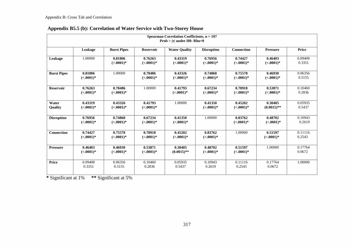
Appendix B: Cross Tab and Correlation
317
Appendix B5.5 (b): Correlation of Water Service with Two-Storey House
Spearman Correlation Coefficients, n = 107
Prob > |r| under H0: Rho=0
Leakage Burst Pipes Reservoir Water Quality Disruption Connection Pressure Price
Leakage 1.00000 0.81806
(<.0001)*
0.76263
(<.0001)*
0.43319
(<.0001)*
0.76956
(<.0001)*
0.74427
(<.0001)*
0.46403
(<.0001)*
0.09408
0.3351
Burst Pipes 0.81806
(<.0001)*
1.00000 0.78486
(<.0001)*
0.43326
(<.0001)*
0.74868
(<.0001)*
0.75578
(<.0001)*
0.46930
(<.0001)*
0.06356
0.5155
Reservoir 0.76263
(<.0001)*
0.78486
(<.0001)*
1.00000 0.41793
(<.0001)*
0.67234
(<.0001)*
0.70918
(<.0001)*
0.53871
(<.0001)*
0.10460
0.2836
Water
Quality
0.43319
(<.0001)*
0.43326
(<.0001)*
0.41793
(<.0001)*
1.00000 0.41350
(<.0001)*
0.45202
(<.0001)*
0.30405
(0.0015)**
0.05935
0.5437
Disruption 0.76956
(<.0001)*
0.74868
(<.0001)*
0.67234
(<.0001)*
0.41350
(<.0001)*
1.00000 0.83762
(<.0001)*
0.48702
(<.0001)*
0.10943
0.2619
Connection 0.74427
(<.0001)*
0.75578
(<.0001)*
0.70918
(<.0001)*
0.45202
(<.0001)*
0.83762
(<.0001)*
1.00000 0.51597
(<.0001)*
0.11116
0.2543
Pressure 0.46403
(<.0001)*
0.46930
(<.0001)*
0.53871
(<.0001)*
0.30405
(0.0015)**
0.48702
(<.0001)*
0.51597
(<.0001)*
1.00000 0.17764
0.0672
Price 0.09408
0.3351
0.06356
0.5155
0.10460
0.2836
0.05935
0.5437
0.10943
0.2619
0.11116
0.2543
0.17764
0.0672
1.00000
* Significant at 1% ** Significant at 5%

Appendix B: Cross Tab and Correlation
318
Appendix B5.5 (c): Correlation of Water Service with Semi-Detached House
Spearman Correlation Coefficients, n = 29
Prob > |r| under H0: Rho=0
Leakage Burst Pipes Reservoir Water Quality Disruption Connection Pressure Price
Leakage 1.00000 0.86349
(<.0001)*
0.84440
(<.0001)*
0.17441
0.3655 0.46013
(0.0120)**
0.52360
(0.0036)**
0.41261
(0.0261)**
0.36713
0.0501
Burst Pipes 0.86349
(<.0001)*
1.00000 0.84922
(<.0001)*
0.23000
0.2300 0.60591
(0.0005)*
0.66312
(<.0001)*
0.42263
0.0224
0.25511
0.1817
Reservoir 0.84440
(<.0001)*
0.84922
(<.0001)*
1.00000 0.16066
0.4051 0.61127
(0.0004)*
0.66743
(<.0001)*
0.44908
(0.0145)**
0.32447
0.0859
Water
Quality
0.17441
0.3655
0.23000
0.2300
0.16066
0.4051
1.00000 0.44958
(0.0144)**
0.47043
(0.0100)**
0.41418
(0.0255)**
-0.16764
0.3847
Disruption 0.46013
(0.0120)**
0.60591
(0.0005)*
0.61127
(0.0004)*
0.44958
(0.0144)**
1.00000 0.93828
(<.0001)*
0.68088
(<.0001)*
0.20505
0.2860
Connection 0.52360
(0.0036)**
0.66312
(<.0001)*
0.66743
(<.0001)*
0.47043
(0.0100)**
0.93828
(<.0001)*
1.00000 0.62111
(0.0003)*
0.24158
0.2068
Pressure 0.41261
(0.0261)**
0.42263
(0.0224)**
0.44908
(0.0145)**
0.41418
0.0255 0.68088
(<.0001)*
0.62111
(0.0003)*
1.00000 0.14511
0.4526
Price 0.36713
0.0501
0.25511
0.1817
0.32447
0.0859
-0.16764
0.3847
0.20505
0.2860
0.24158
0.2068
0.14511
0.4526
1.00000
* Significant at 1% ** Significant at 5%

Appendix B: Cross Tab and Correlation
319
Appendix B5.5 (d): Correlation of Water Service with Bungalow
Spearman Correlation Coefficients, n = 31
Prob > |r| under H0: Rho=0
Leakage Burst Pipes Reservoir Water Quality Disruption Connection Pressure Price
Leakage 1.00000 0.68216
(<.0001)*
0.46433
(0.0085)**
0.61437
(0.0002)*
0.37064
(0.0401)**
0.46768
(0.0080)**
0.64386
(<.0001)*
-0.11056
0.5538
Burst Pipes 0.68216
(<.0001)*
1.00000 0.52744
(0.0023)**
0.61583
(0.0002)*
0.42885
(0.0161)**
0.43762
(0.0138)**
0.62118
(0.0002)*
-0.10670
0.5678
Reservoir 0.46433
(0.0085)**
0.52744
(0.0023)**
1.00000 0.24593
0.1823 0.44547
(0.0120)**
0.25210
0.1713
0.25518
0.1659
0.10945
0.5578
Water
Quality
0.61437
(0.0002)*
0.61583
(0.0002)*
0.24593
0.1823
1.00000 0.33809
0.0628 0.49628
(0.0045)**
0.58644
(0.0005)*
-0.26073
0.1566
Disruption 0.37064
(0.0401)**
0.42885
(0.0161)**
0.44547
(0.0120)**
0.33809
0.0628
1.00000 0.47207
(0.0073)**
0.44183
(0.0128)**
0.13449
0.4707
Connection 0.46768
(0.0080)**
0.43762
(0.0138)**
0.25210
0.1713 0.49628
(0.0045)**
0.47207
(0.0073)**
1.00000 0.76844
(<.0001)*
0.20949
0.2580
Pressure 0.64386
(<.0001)*
0.62118
(0.0002)*
0.25518
0.1659 0.58644
(0.0005)*
0.44183
(0.0128)**
0.76844
(<.0001)*
1.00000 0.14302
0.4428
Price -0.11056
0.5538
-0.10670
0.5678
0.10945
0.5578
-0.26073
0.1566
0.13449
0.4707
0.20949
0.2580
0.14302
0.4428
1.00000
* Significant at 1% ** Significant at 5%

Appendix B: Cross Tab and Correlation
320
Appendix B5.5 (e): Correlation of Water Service with Others
Spearman Correlation Coefficients, n = 80
Prob > |r| under H0: Rho=0
Leakage Burst Pipes Reservoir Water Quality Disruption Connection Pressure Price
Leakage 1.00000 0.90354
(<.0001)*
0.76752
(<.0001)*
0.48175
(<.0001)*
0.65006
(<.0001)*
0.60479
(<.0001)*
0.55989
(<.0001)*
0.19398
0.0847
Burst Pipes 0.90354
(<.0001)*
1.00000 0.76752
(<.0001)*
0.42595
(<.0001)*
0.69653
(<.0001)*
0.58197
(<.0001)*
0.62876
(<.0001)*
0.19398
0.0847
Reservoir 0.76752
(<.0001)*
0.76752
(<.0001)*
1.00000 0.45957
(<.0001)*
0.78988
(<.0001)*
0.54239
(<.0001)*
0.68137
(<.0001)*
0.20839
0.0636
Water
Quality
0.48175
(<.0001)*
0.42595
(<.0001)*
0.45957
(<.0001)*
1.00000 0.43499
(<.0001)*
0.39322
(0.0003)*
0.39635
(0.0003)*
0.13394
0.2362
Disruption 0.65006
(<.0001)*
0.69653
(<.0001)*
0.78988
(<.0001)*
0.43499
(<.0001)*
1.00000 0.67322
(<.0001)*
0.63762
(<.0001)*
0.22451
(0.0453)**
Connection 0.60479
(<.0001)*
0.58197
(<.0001)*
0.54239
(<.0001)*
0.39322
(0.0003)*
0.67322
(<.0001)*
1.00000 0.71449
(<.0001)*
0.20711
0.0653
Pressure 0.55989
(<.0001)*
0.62876
(<.0001)*
0.68137
(<.0001)*
0.39635
(0.0003)*
0.63762
(<.0001)*
0.71449
(<.0001)*
1.00000 0.20438
0.0690
Price 0.19398
0.0847
0.19398
0.0847
0.20839
0.0636
0.13394
0.2362
0.22451
0.0453
0.20711
0.0653
0.20438
0.0690
1.00000
* Significant at 1% ** Significant at 5%

Appendix B: Cross Tab and Correlation
321
Appendix B6
Appendix B6.1 (a): Correlation of Strategies with Malay
Spearman Correlation Coefficients, n = 329
Prob > |r| under H0: Rho=0
Integrated Training Funding Education
Integrated 1.00000 0.67452 0.69341 0.67434
(<.0001)* (<.0001)* (<.0001)*
Training 0.67452 1.00000 0.68304 0.67448
(<.0001)* (<.0001)* (<.0001)*
Funding 0.69341 0.68304 1.00000 0.72553
(<.0001)* (<.0001)* (<.0001)*
Education 0.67434 0.67448 0.72553 1.00000
(<.0001)* (<.0001)* (<.0001)*
* Significant at 1%
Appendix B6.1 (b): Correlation of Strategies with Chinese
Spearman Correlation Coefficients, n = 48
Prob > |r| under H0: Rho=0
Integrated Training Funding Education
Integrated 1.00000 0.91858 0.96386 0.92938
(<.0001)* (<.0001)* (<.0001)*
Training 0.91858 1.00000 0.88155 0.87619
(<.0001)* (<.0001)* (<.0001)*
Funding 0.96386 0.88155 1.00000 0.89032
(<.0001)* (<.0001)* (<.0001)*
Education 0.92938 0.87619 0.89032 1.00000
(<.0001)* (<.0001)* (<.0001)*
* Significant at 1%

Appendix B: Cross Tab and Correlation
322
Appendix B6.1 (c): Correlation of Strategies with Indian
Spearman Correlation Coefficients, n = 11
Prob > |r| under H0: Rho=0
Integrated Training Funding Education
Integrated 1.00000 1.0000 1.0000 0.81009
(<.0001)* (<.0001)* (<.0025)*
Training 1.00000 1.00000 1.0000 0.81009
(<.0001)* (<.0001)* (<.0025)*
Funding 1.00000 1.0000 1.00000 0.81009
(<.0001)* (<.0001)* (<.0025)*
Education 0.81009 0.81009 0.81009 1.00000
(<.0025)* (<.0025)* (<.0025)*
* Significant at 1%
Appendix B6.1 (d): Correlation of Strategies with Others
Spearman Correlation Coefficients, n = 4
Prob > |r| under H0: Rho=0
Integrated Training Funding Education
Integrated 1.00000 0.81650 0.81650 0.81650
0.1835 0.1835 0.1835
Training 0.81650 1.00000 0.33333 1.00000
0.1835 0.6667 <.0001*
Funding 0.81650 0.33333 1.00000 0.33333
0.1835 0.6667 0.6667
Education 0.81650 1.00000 0.33333 1.00000
0.1835 <.0001* 0.6667
* Significant at 1%

Appendix B: Cross Tab and Correlation
323
Appendix B6.2 (a): Correlation of Strategies with Age (20 to 30 years)
Pearson Correlation Coefficients, n = 151
Prob > |r| under H0: Rho=0
Integrated Training Funding Education
Integrated 1.00000 0.55110 0.58783 0.58291
(<.0001)* (<.0001)* (<.0001)*
Training 0.55110 1.00000 0.67146 0.57964
(<.0001)* (<.0001)* (<.0001)*
Funding 0.58783 0.67146 1.00000 0.62048
(<.0001)* (<.0001)* (<.0001)*
Education 0.58291 0.57964 0.62048 1.00000
(<.0001)* (<.0001)* (<.0001)*
* Significant at 1%
Appendix B6.2 (b): Correlation of Strategies with Age (31 to 40 years)
Pearson Correlation Coefficients, n = 75
Prob > |r| under H0: Rho=0
Integrated Training Funding Education
Integrated 1.00000 0.73780 0.72457 0.69389
(<.0001)* (<.0001)* (<.0001)*
Training 0.73780 1.00000 0.65416 0.75025
(<.0001)* (<.0001)* (<.0001)*
Funding 0.72457 0.65416 1.00000 0.74000
(<.0001)* (<.0001)* (<.0001)*
Education 0.69389 0.75025 0.74000 1.00000
(<.0001)* (<.0001)* (<.0001)*
* Significant at 1%

Appendix B: Cross Tab and Correlation
324
Appendix B6.2 (c): Correlation of Strategies with Age (41 to 50 years)
Pearson Correlation Coefficients, n = 83
Prob > |r| under H0: Rho=0
Integrated Training Funding Education
Integrated 1.00000 0.76521 0.76740 0.84217
(<.0001)* (<.0001)* (<.0001)*
Training 0.76521 1.00000 0.71091 0.68957
(<.0001)* (<.0001)* (<.0001)*
Funding 0.76740 0.71091 1.00000 0.80950
(<.0001)* (<.0001)* (<.0001)*
Education 0.84217 0.68957 0.80950 1.00000
(<.0001)* (<.0001)* (<.0001)*
* Significant at 1%
Appendix B6.2 (d): Correlation of Strategies with Age (More than 51 years)
Pearson Correlation Coefficients, n = 83
Prob > |r| under H0: Rho=0
Integrated Training Funding Education
Integrated 1.00000 0.76310 0.65987 0.69594
(<.0001)* (<.0001)* (<.0001)*
Training 0.76310 1.00000 0.67939 0.69233
(<.0001)* (<.0001)* (<.0001)*
Funding 0.65987 0.67939 1.00000 0.78153
(<.0001)* (<.0001)* (<.0001)*
Education 0.69594 0.69233 0.78153 1.00000
(<.0001)* (<.0001)* (<.0001)*
* Significant at 1%

Appendix B: Cross Tab and Correlation
325
Appendix B6.3 (a): Correlation of Strategies with Child (2 children or fever)
Pearson Correlation Coefficients, n = 214
Prob > |r| under H0: Rho=0
Integrated Training Funding Education
Integrated 1.00000 0.65941 0.69745 0.65710
(<.0001)* (<.0001)* (<.0001)*
Training 0.65941 1.00000 0.65865 0.58526
(<.0001)* (<.0001)* (<.0001)*
Funding 0.69745 0.65865 1.00000 0.67979
(<.0001)* (<.0001)* (<.0001)*
Education 0.65710 0.58526 0.67979 1.00000
(<.0001)* (<.0001)* (<.0001)*
*Significant at 1%
Appendix B6.3 (b): Correlation of Strategies with Child (3 to 5 children)
Pearson Correlation Coefficients, n = 122
Prob > |r| under H0: Rho=0
Integrated Training Funding Education
Integrated 1.00000 0.71365 0.60980 0.66850
(<.0001)* (<.0001)* (<.0001)*
Training 0.71365 1.00000 0.68668 0.78526
(<.0001)* (<.0001)* (<.0001)*
Funding 0.60980 0.68668 1.00000 0.78631
(<.0001)* (<.0001)* (<.0001)*
Education 0.66850 0.78526 0.78631 1.00000
(<.0001)* (<.0001)* (<.0001)*
*Significant at 1%

Appendix B: Cross Tab and Correlation
326
Appendix B6.3 (c): Correlation of Strategies with Child (6 to 8 children)
Pearson Correlation Coefficients, n = 41
Prob > |r| under H0: Rho=0
Integrated Training Funding Education
Integrated 1.00000 0.50278 0.54215 0.81732
(<.0001)* (<.0001)* (<.0001)*
Training 0.50278 1.00000 0.80429 0.66746
(<.0001)* (<.0001)* (<.0001)*
Funding 0.54215 0.80429 1.00000 0.73580
(<.0001)* (<.0001)* (<.0001)*
Education 0.81732 0.66746 0.73580 1.00000
(<.0001)* (<.0001)* (<.0001)*
*Significant at 1%
Appendix B6.3 (d): Correlation of Strategies with Child (More than 9 children)
Pearson Correlation Coefficients, n = 11
Prob > |r| under H0: Rho=0
Integrated Training Funding Education
Integrated 1.00000 0.82808 0.91147 0.91147
(0.0016)* (<.0001)* (<.0001)*
Training 0.82808 1.00000 0.81242 0.81242
(0.0016)* (0.0024)* (0.0024)*
Funding 0.91147 0.81242 1.00000 1.00000
(<.0001)* (0.0024)* (<.0001)*
Education 0.91147 0.81242 1.00000 1.00000
(<.0001)* (0.0024)* (<.0001)*
*Significant at 1%

Appendix B: Cross Tab and Correlation
327
Appendix B6.4 (a): Correlation of Strategies with Person (2 persons or fewer)
Pearson Correlation Coefficients, n = 67
Prob > |r| under H0: Rho=0
Integrated Training Funding Education
Integrated 1.00000 0.85472 0.72188 0.81279
(<.0001)* (<.0001)* (<.0001)*
Training 0.85472 1.00000 0.70973 0.70728
(<.0001)* (<.0001)* (<.0001)*
Funding 0.72188 0.70973 1.00000 0.59612
(<.0001)* (<.0001)* (<.0001)*
Education 0.81279 0.70728 0.59612 1.00000
(<.0001)* (<.0001)* (<.0001)*
*Significant at 1%
Appendix B6.4 (b): Correlation of Strategies with Person (3 to 5 persons)
Pearson Correlation Coefficients, n = 180
Prob > |r| under H0: Rho=0
Integrated Training Funding Education
Integrated 1.00000 0.66286 0.62117 0.58406
(<.0001)* (<.0001)* (<.0001)*
Training 0.66286 1.00000 0.64426 0.68726
(<.0001)* (<.0001)* (<.0001)*
Funding 0.62117 0.64426 1.00000 0.73587
(<.0001)* (<.0001)* (<.0001)*
Education 0.58406 0.68726 0.73587 1.00000
(<.0001)* (<.0001)* (<.0001)*
*Significant at 1%

Appendix B: Cross Tab and Correlation
328
Appendix B6.4 (c): Correlation of Strategies with Person (6 to 8 persons)
Pearson Correlation Coefficients, n = 113
Prob > |r| under H0: Rho=0
Integrated Training Funding Education
Integrated 1.00000 0.59922 0.77497 0.77063
(<.0001)* (<.0001)* (<.0001)*
Training 0.59922 1.00000 0.71639 0.56130
(<.0001)* (<.0001)* (<.0001)*
Funding 0.77497 0.71639 1.00000 0.78907
(<.0001)* (<.0001)* (<.0001)*
Education 0.77063 0.56130 0.78907 1.00000
(<.0001)* (<.0001)* (<.0001)*
*Significant at 1%
Appendix B6.4 (d): Correlation of Strategies with Person (More than 9 persons)
Pearson Correlation Coefficients, n = 31
Prob > |r| under H0: Rho=0
Integrated Training Funding Education
Integrated 1.00000 0.55574 0.37516 0.61608
(0.0012)* 0.0376 (0.0002)*
Training 0.55574 1.00000 0.68596 0.66672
(0.0012)* (<.0001)* (<.0001)*
Funding 0.37516 0.68596 1.00000 0.61693
0.0376 (<.0001)* (<.0002)*
Education 0.61608 0.66672 0.61693 1.00000
(0.0002)* (<.0001)* (0.0002)*
*Significant at 1%

Appendix B: Cross Tab and Correlation
329
Appendix B6.5 (a): Correlation of Strategies with Terraced House
Spearman Correlation Coefficients, n = 145
Prob > |r| under H0: Rho=0
Integrated Training Funding Education
Integrated 1.00000 0.74363 0.78529 0.71280
(<.0001)* (<.0001)* (<.0001)*
Training 0.74363 1.00000 0.59737 0.68253
(<.0001)* (<.0001)* (<.0001)*
Funding 0.78529 0.59737 1.00000 0.71352
(<.0001)* (<.0001)* (<.0001)*
Education 0.71280 0.68253 0.71352 1.00000
(<.0001)* (<.0001)* (<.0001)*
*Significant at 1%
Appendix B6.5 (b): Correlation of Strategies with Two-Storey House
Spearman Correlation Coefficients, n = 107
Prob > |r| under H0: Rho=0
Integrated Training Funding Education
Integrated 1.00000 0.70209 0.72513 0.72611
(<.0001)* (<.0001)* (<.0001)*
Training 0.70209 1.00000 0.76332 0.79542
(<.0001)* (<.0001)* (<.0001)*
Funding 0.72513 0.76332 1.00000 0.77097
(<.0001)* (<.0001)* (<.0001)*
Education 0.72611 0.79542 0.77097 1.00000
(<.0001)* (<.0001)* (<.0001)*
*Significant at 1%

Appendix B: Cross Tab and Correlation
330
Appendix B6.5 (c): Correlation of Strategies with Semi-Detached House
Spearman Correlation Coefficients, n = 29
Prob > |r| under H0: Rho=0
Integrated Training Funding Education
Integrated 1.00000 0.61488 0.73193 0.58082
(0.0004)* (<.0001)* (0.0010)*
Training 0.61488 1.00000 0.70563 0.55381
(0.0004)* (<.0001)* (0.0018)*
Funding 0.73193 0.70563 1.00000 0.78195
(<.0001)* (<.0001)* (<.0001)*
Education 0.58082 0.55381 0.77097 1.00000
(0.0010)* (0.0018)* (<.0001)*
*Significant at 1%
Appendix B6.5 (d): Correlation of Strategies with Bungalow
Spearman Correlation Coefficients, n = 31
Prob > |r| under H0: Rho=0
Integrated Training Funding Education
Integrated 1.00000 0.66982 0.54163 0.58020
(<.0001)* (0.0017)* (0.0006)*
Training 0.66982 1.00000 0.80144 0.70901
(<.0001)* (<.0001)* (<.0001)*
Funding 0.54163 0.80144 1.00000 0.69465
(0.0017)* (<.0001)* (<.0001)*
Education 0.58020 0.70901 0.69465 1.00000
(0.0006)* (<.0001)* (<.0001)*
*Significant at 1%

Appendix B: Cross Tab and Correlation
331
Appendix B6.5 (e): Correlation of Strategies with Others
Spearman Correlation Coefficients, n = 80
Prob > |r| under H0: Rho=0
Integrated Training Funding Education
Integrated 1.00000 0.72894 0.73928 0.77077
(<.0001)* (<.0001)* (<.0001)*
Training 0.72894 1.00000 0.77436 0.66293
(<.0001)* (<.0001)* (<.0001)*
Funding 0.73928 0.77436 1.00000 0.75006
(<.0001)* (<.0001)* (<.0001)*
Education 0.77077 0.66293 0.75006 1.00000
(<.0001)* (<.0001)* (<.0001)*
*Significant at 1%