ASSESSING THE ACCURACY OF AUSTRALIA'S SMALL-AREA POPULATION ESTIMATES

ASSESSING THE ACCURACY OF AUSTRALIA'S SMALL-AREA POPULATION ESTIMATESAuthor(s): Andrew HoweSource: Journal of the Australian Population Association, Vol. 16, No. 1/2 (May 1999), pp. 47-63Published by: SpringerStable URL: http://www.jstor.org/stable/41110477 .

Accessed: 15/06/2014 21:03

Your use of the JSTOR archive indicates your acceptance of the Terms & Conditions of Use, available at .http://www.jstor.org/page/info/about/policies/terms.jsp

.JSTOR is a not-for-profit service that helps scholars, researchers, and students discover, use, and build upon a wide range ofcontent in a trusted digital archive. We use information technology and tools to increase productivity and facilitate new formsof scholarship. For more information about JSTOR, please contact [email protected].

.

Springer is collaborating with JSTOR to digitize, preserve and extend access to Journal of the AustralianPopulation Association.

http://www.jstor.org

This content downloaded from 62.122.73.86 on Sun, 15 Jun 2014 21:03:33 PMAll use subject to JSTOR Terms and Conditions

http://www.jstor.org/action/showPublisher?publisherCode=springer

http://www.jstor.org/stable/41110477?origin=JSTOR-pdf

http://www.jstor.org/page/info/about/policies/terms.jsp


Vol.16. Nos.1/2, 1999 Journal of the Australian Population Association

ASSESSING THE ACCURACY OF AUSTRALIA'S SMALL-AREA POPULATION ESTIMATES

Andrew Howe Small Area Population Unit

Australian Bureau of Statistics GPO Box 2272, Adelaide 5001

[email protected]

The Australian Bureau of Statistics provides population estimates of Statistical Local Areas annually. The accuracy of these estimates can be assessed after population estimates are rebased after each quinquennial Census of Population and Housing, however there appears to be no

straightforward method of assessing these estimates. Errors that occur with population estimates can be attributed to several factors, both broad and specific to individual areas. These factors include inherent characteristics of the region, such as population si2e and growth rate; changes in the geographic boundaries; quality of input data; estimation method; and adjustments to control totals (state populations).

The Australian Bureau of Statistics (ABS) compiles and publishes estimates of the population and its components. Here, population is defined according to the concept of Estimated Resident Population (ERP), which links people to their place of usual residence within Australia. ERPs are produced annually for Statistical Local Areas (SLAs). The SLA is the base spatial unit used to collect and disseminate statistics other than those collected from the Census of Population and Housing. In aggregate, SLAs cover the whole of Australia without gaps or overlaps. SLAs generally conform to or combine to form Local Government Areas (LGAs). SLA population estimates are produced annually, on 30 June.

This paper describes and assesses some of the broader - and sometimes inherent - factors behind errors in small-area population estimates, in the context of the 1996 Australian Statistical Local Area populations. Population estimators may then take these factors into account when estimating small-area populations. Similarly, users of population data may know what to take into account when using such small-area data.

The ERPs in SLAs are used extensively for the planning of provision of goods, services and infrastructure throughout the public and private sectors. In addition, SLA population estimates are used as a base for population projections. Users of these small-area estimates and projections include business planners, health analysts, grants bodies and electoral commissions.

47



Methods of Estimation The method used to produce the annual SLA population estimates depends

on whether a Census of Population and Housing was conducted that year. AU SLA population estimates are constrained to add to their previously derived state population total.

Censusyears Census data are predominandy used to produce ERPs for SLAs on 30 June

of the census year. Census counts of usual residents by SLA are adjusted for undercounting using data from the census Post-Enumeration Survey.1 Adjust- ments are also made by estimating the number of Australian residents temporarily overseas, derived from residential addresses reported by these residents on passenger cards upon returning to Australia after a census. If the census does not occur on 30 June (for example the 1996 Census was held on 6 August) then a further adjustment is made to produce estimates at 30 June. Estimates produced in this way are referred to as final ERPs.

Non-census years Based on the census year estimates, SLA population estimates are updated

as at 30 June in following years. Although annual births and deaths data are available for SLAs, the absence of migration data for non-census years means that it is not possible to use the component method to update SLA population totals.

Before 1996, SLA population estimates for non-census years were calculated by the state2 ABS offices, using a variety of procedures and techniques. Regres- sion techniques first establish a relationship, based on past data, between population change (usually percentage share of state total) and the change in symptomatic indicators, which are any available set of data which in some way relates to changes in population size. The choice of symptomatic indicators varies across the states. Examples include dwellings, Medicare enrolments, drivers' licences and electricity connections. The relationships between the change in population and symptomatic indicators are expressed mathematically in terms of regression coefficients which, with the knowledge of the change in the indicators for the current time period, enable population change to be estimated. This estimation procedure is well documented and is used extensively overseas (ABS 1982, 1995; McCullagh and Zidek 1988; Statistics 1 The Post-Enumeration Survey is a sample survey conducted immediately after the census to estimate the number of people (and their characteristics) who did not complete or were not included on a census form. It also detects instances of double counting of individuals, but the number of such cases is far outweighed by the number of people who arc not counted The net undercount is therefore the excess of the undercount (people not counted) over the number of instances of double counting. In 1996 the net undercount for Australia was 1.6 per cent

(ABS 1997a). 2 In this paper the term 'state1 refers to Australia's states and territories.

48



Canada 1992; US Bureau of the Census 1994). Because there can be considerable differences between SLAs in the relation-

ship between symptomatic indicators and population, stratification is applied to the modelling procedure. This involves separating the SLAs within a state into subsets based on factors such as location (for example urban or rural), population growth (high or low), and the house per dwelling ratio. More accurate estimates may then be calculated based on relationships existing within these subsets of more homogeneous SLAs.

At the conclusion of the modelling stage, each population estimate is scrutinized on the basis of local knowledge, alternative procedures or other data sources. Subjective adjustments to modelled estimates are sometimes made. These non-census year estimates are called preliminary estimates; they are also produced for census years prior to census data being available.

Assessment of Accuracy To assess the accuracy of the estimates, a comparison can be made between

the preliminary and final SLA population estimates for census years. For instance, the 1996 SLA estimates based on the 1991 Census (preliminary) can be compared with the 1996 estimates finalized from the 1996 Census (final). The census-based (final) 1996 estimates are implicidy assumed to be correct The difference between preliminary and final ERPs for each SLA is a measure of intercensal error, sometimes referred to as the intercensal discrepancy or the estimation error.

The intercensal error is a valuable tool for assessing the quality of ERPs produced since the previous census. Thus the 30 June 1996 intercensal errors not only measure differences between preliminary and final ERPs in 1996, but also reflect the accuracy or otherwise of population estimates for 1992 to 1995.

Measures of intercensal error Several measures of the intercensal error can be considered. The most

common measure is a percentage difference. However, a numeric difference may also be useful. Other measures can be obtained by transforming the scale, for example, by using a logarithmic scale. There are advantages and disadvan- tages in each approach.

The wide range in SLA size means that in the process of evaluating intercensal errors, care should be taken to ensure that no particular group of SLAs (in terms of size) is disadvantaged by conclusions made for other groups. Evaluation based purely on one measure of error assumes that a given error carries the same significance, despite the range of SLA size. Table 1 considers various measures of error associated with populations of size 2,000, 20,000 and 200,000. It can be seen that different measures lead to potentially different conclusions about accuracy depending on population size.

Percentage errors are not suited to the analysis of SLAs covering a wide range of population sizes because percentage errors are generally greater for

49



Table 1 Examples of errors and measures of error associated with populations of si2e 2,000, 20,000 and 200,000

Final ERP Preliminary ERP Percentage error Numeric error Log error

Percentage error = +5 per cent 2,000 2,100 5.0 100 0.61

20,000 21,000 5.0 1,000 0.70 200,000 210,000 5.0 10,000 0.75

Numeric error = +1,000 persons 2,000 3,000 50.0 1,000 0.91

20,000 21,000 5.0 1,000 0.70 200,000 201,000 0.5 1,000 0.57

Log error = 0.67 2,000 2,163 8.1 163 0.67

20,000 20,762 3.8 762 0.67 200,000 203,562 ^8 3,562 0.67

Note: Percentage error = 100 x (Pp - Pf)/Pf

Numeric error = Pp - Pf

Log error = log | Pp - Pf | /log(PÒ

where Pp = preliminary ERP and Pf = final ERP.

small SLAs. Similarly, numeric errors are not suited to SLAs covering a wide range of population sizes because numeric errors are generally greater for large SLAs. A logarithmic transformation may be considered a compromise between

percentage and numeric errors, because population size has a reduced effect An important consideration when evaluating these errors is the effect of

error in one area estimate on error in other area estimates due to the constraint that estimates sum to total population at the state level. This is especially relevant when funds are allocated on the basis of share of total state

population. For instance, if a relatively large LGA was significantly overestimated, then the remaining LGAs would receive a smaller share of the available pool of funding. Nash (1950) attempted to account for this by deriving a criterion function which recognizes the need to choose an allocation scheme which is a joindy acceptable compromise for all members of a

community. This function suggests that the chi-squared statistic may be the most appropriate measure of error.

Despite its shortcomings, the traditional measure of intercensal error is the

percentage error. When a number of errors are combined to produce a

summary statistic such as the average SLA intercensal error for a state, the absolute value of the error must be used to avoid counterbalancing. The impact on summary measures of the tendency for percentage error to overemphasize the degree of error for small SLAs may be reduced by simply excluding very small SLAs from analysis. In evaluating the accuracy of population estimates, the remainder of this paper will focus mainly on the percentage error,

50



Distribution of SLA Size The nature of SLA geography across Australia is such that SLAs range in

size from zero to well over 200,000 persons. The SLA with the largest population in 1996 was Blacktown, in the northwest of Sydney, with 239,818 persons. Larger SLAs tend to lie in urban areas. Several SLAs had zero populations in 1996. The SLAs included in this analysis are those as defined in the 1996 version of the Australian Standard Geographical Classification (ABS 1996).

Table 2 shows the distribution of SLA population size by state in 1996. It is seen that for all states, the mean ERP equals or exceeds the median. Six states had a mean ERP much larger than the median, indicating that in those states, a relatively small number of SLAs had a relatively large proportion of the population. In fact, over 50 per cent of the population of South Australia and Western Australia resided in only eight and nine per cent of the SLAs respectively. At the other extreme, the Australian Capital Territory and the Northern Territory (where the median SLA size was much closer to the average SLA size) had half of their population in 27 and 25 per cent of SLAs respectively. Table 2 Statistical Local Areas by population size by state, 30 June 1996

Population size Mean Median Statc Õtõ 500 to 1,000 to 5,000 to 10,000 to 50,000 Total ^^ ERP

99 999 4,999 9,999 49,999 and over number C000) C000)

NSW 4 2 52 33 57 41 189 32.8 10.9 Vic 5 2 37 48 84 24 200 22.8 10.3 Qld 19 20 169 130 108 3 449 7.4 5.4 SA 12 7 56 23 26 6 130 11.3 3.5 WA 13 24 54 18 32 10 151 11.7 2.6 Tas 3 3 13 12 12 1 44 10.8 5.9 NT 3 6 45 8 1 0 63 2.9 2.4 ACT 20 5 70 11 1 0 107 2.9 2.9 Australia 79 69 496 283 321 85 1,333 13.7 4.0

Source: Author's computations using data from ABS (1998a).

Assessment of 1996 Population Estimates The estimated resident population of Australia at 30 June 1996 derived by

updating the previous census fell short of the 1996 census-based population by 21,572 persons.3 In other words, the intercensal error was -21,572, or -0.1 per cent, at the national level. The size and direction of errors varied between states. New South Wales had an error of -14,500 persons (-0.2 per cent of the state's final population), Victoria -19,200 (-0.4 per cent), Queensland +16,000 (+0.5 per cent), South Australia +4,900 (+0.3 per cent), Western Australia ** When final births, deaths and migrant category jumping became available, the national intercensal discrepancy was revised to -27,500 (ABS 1998b). SLAs were not updated this way.

51



-2,600 (-0.1 per cent), Tasmania -1,000 (-0.2 per cent), Northern Territory -4,100 (-2.4 per cent) and Australian Capital Territory -800 (-0.2 per cent).

Statistical Local Areas

Despite an underestimate of the total Australian population, a larger number of SLA totals were overestimated (positive intercensal error) than were underestimated (negative intercensal error) as Table 3 shows. The number of overestimated SLAs was 709, while 607 were underestimated. The overall underestimate of the national population combined with the fact that a majority of SLAs were overestimated equates to smaller SLAs being overestimated more frequently than larger SLAs.

Table 3 Statistical Local Areas by size of intercensal error by state, 30 June 1996

Intercensal error State _5o/o and >.5 to >-2to >0to 2to 5% and Total

under -2% <0% <2% <5% over

NSW 37 43 43 30 23 10 186 Vic 31 35 38 36 28 29 197

Qld 86 78 78 72 75 58 447 SA 8 15 34 29 26 15 127 WA 32 18 26 34 19 21 150 Tas 4 4 14 8 6 7 43 NT io 7 6 8 9 22 62 ACT 22 20 17 16 17 14 106 Australia 230 220 256 233 203 176 1,318

Notes: Excludes SLAs where preliminary and final ERP was zero. Percentage errors for SLAs with non-zero preliminary ERP and zero final ERP are undefined. Some SLAs were combined to conform with published preliminary ERPs. Five SLAs had zero intercensal error in 1996.

Source: Author's computations using data from ABS.

Across Australia, there were 912, or 69 per cent of SLAs with a 1996 intercensal error of less than five per cent. In each state except the Northern

Territory, 65 per cent or more of preliminary SLA estimates were less than five

per cent in error. South Australia had the highest percentage of SLAs with less than five per cent error (104 SLAs, or 82 per cent), while Northern Territory had the lowest percentage (30 SLAs, or 48 per cent). Tasmania had the highest percentage with errors of less than two per cent (22 SLAs, or 51 per cent).

As mentioned previously, to include very small SLAs in the calculation of

average error for states may result in misleading conclusions. For example, the SLA of Kowen, a sparsely populated SLA on the outskirts of the Australian

Capital Territory, had a preliminary 1996 estimate of 47 persons - close to its 1991 estimate of 50 persons. However, the final 1996 ERP for Kowen was 16. The intercensal error for Kowen was therefore 194 per cent, or 31 persons. Given that this was a tiny SLA (in terms of population), this further confirms

52



that, in the case of very small SLAs, a large percentage error does not necessarily imply a large numeric error. To include these very small SLAs which are more prone to high percentage errors, of which there are several in the ACT, would give an unfair representation of the performance of SLA population estimates in this state. For this reason, SLAs in all states with a finalized 1996 population less than 500 are excluded in the calculation of average absolute percentage errors in some parts of this paper. The total number of persons residing in these SLAs in 1996 was less than 0.1 per cent of the total Australian population.

Local Government Areas The analysis of population estimates for LGAs is important given that

allocation of funds by governments often depends on the distribution of LGA populations. In 1996, die LGA structure closely resembled the SLA structure in New South Wales, South Australia and Western Australia. Hence for these three states, the patterns observed with LGA population errors are similar to those errors associated with SLA population estimates.

Parts of state Each state can be divided into its Capital City (Statistical Division) and Ttest

of State'. Overall, the capital cities were underestimated by 96,400 persons, or -0.8 per cent. The population outside capital cities was overestimated by almost 74,700, or +1.1 per cent

Later parts of this paper discuss the fact that smaller and declining SLAs tend to be overestimated. SLAs located in rural areas are generally small, and declining SLAs tend to be located in rural areas. These two factors appear to contribute to the liest of States' (mainly rural areas) being overestimated.

Factors Affecting the Accuracy of SLA Population Estimates Several factors can influence the accuracy of an SLA population estimate.

This section attempts to identify some underlying characteristics and factors of SLAs that potentially hinder the accuracy of population estimates. This is done by assessing the 1996 SLA intercensal errors using percentage errors.

Population si%e As already indicated, larger populations tend to be more accurately estimated

than small populations, when the measure of accuracy is percentage error. This is seen in Figure 1 which shows average absolute percentage error by SLA size for 1996. As SLA size increased, there was a steady decline in average percentage error. The average absolute error for SLAs with populations of less than 500 was 23 per cent, and 37 per cent of these SLAs have errors greater than 20 per cent But for SLAs with populations of 50,000 or more, the average error was only two per cent, and only ten per cent of these SLAs had errors of

53



Figure 1 Average absolute percentage intercensal error for Statistical Local Areas by sise of Statistical Local Area, 30 June 1996

25 i - - - - - - - |

20 ■

I 15 ■&

g io ■ ■ -

":1 nli i r ~ - 1 1 - i ■ - ■! <0.5 0.5 -<1 l-<5 5-<10 10-<50 50+

Size of SLA fOOO persons)

Source: Authors computations using data from ABS.

more than five per cent. This trend was also observed in the United States (US Bureau of the Census

1994). For all 3,141 counties in the US in 1990, the average absolute error was 3.6 per cent The 105 counties with a population less than 2,500 had an average error of 7.7 per cent, while the average error for the 414 counties with more than 100,000 persons was 2.0 per cent.

Direction of error is also related to population size. The populations of smaller areas are more likely to be overestimated than the populations of larger areas. Of the SLAs with less than 500 persons, 68 per cent were overestimated. However, of the SLAs with a population more than 50,000, only 46 per cent were overestimated.

Population growth Table 4 shows the distribution of SLAs by population growth, between 1991

and 1996. Figure 2 shows the relationship between average absolute percentage intercensal error in 1996 and population growth between 1991 and 1996. It can be seen that moderately changing populations can be estimated more accurately than rapidly changing populations. 1996 SLA estimates for populations that had declined by more than 10 per cent since 1991 had an average absolute intercensal error of 17.9 per cent For populations that grew by 20 per cent or more, the average error was 8.3 per cent The lowest average error (3.1 per cent) was for populations that grew, but by less than 10 per cent

A similar but less pronounced pattern is seen in the 1990 United States county population estimates. Counties that declined by more than five per cent between 1980 and 1990 had an average error of 3.8 per cent, and those counties

54



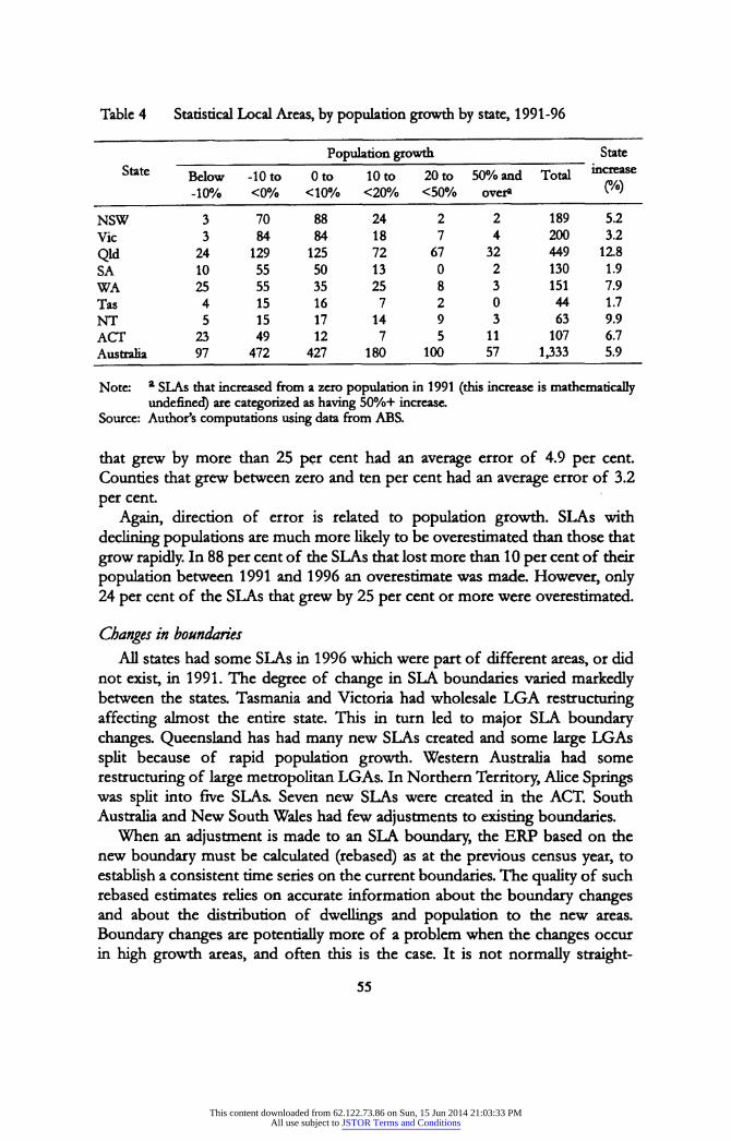
Table 4 Statistical Local Areas, by population growth by state, 1991-96

Population growth State State Below -10 to Oto loto 20to 50% and Total in<^*Se ™0' -10% <0% <10% <20% <50% over* ™0'

NSW 3 70 88 24 2 2 189 5.2 Vic 3 84 84 18 7 4 200 3.2

Qld 24 129 125 72 67 32 449 12.8 SA 10 55 50 13 0 2 130 1.9 WA 25 55 35 25 8 3 151 7.9 Tas 4 15 16 7 2 0 44 1.7 NT 5 15 17 14 9 3 63 9.9 ACT 23 49 12 7 5 11 107 6.7 Australia 97 472 427 180 100 57 1,333 5.9

Note: a SLAs that increased from a zero population in 1991 (this increase is mathematically undefined) are categorized as having 50%+ increase.


that grew by more than 25 pçr cent had an average error of 4.9 per cent. Counties that grew between zero and ten per cent had an average error of 3.2 per cent

Again, direction of error is related to population growth. SLAs with declining populations are much more likely to be overestimated than those that grow rapidly. In 88 per cent of the SLAs that lost more than 10 per cent of their population between 1991 and 1996 an overestimate was made. However, only 24 per cent of the SLAs that grew by 25 per cent or more were overestimated.

Changes in boundaries

All states had some SLAs in 1996 which were part of different areas, or did not exist, in 1991. The degree of change in SLA boundaries varied markedly between the states. Tasmania and Victoria had wholesale LGA restructuring affecting almost the entire state. This in turn led to major SLA boundary changes. Queensland has had many new SLAs created and some large LGAs split because of rapid population growth. Western Australia had some restructuring of large metropolitan LGAs. In Northern Territory, Alice Springs was split into five SLAs. Seven new SLAs were created in the ACT. South Australia and New South Wales had few adjustments to existing boundaries.

When an adjustment is made to an SLA boundary, the ERP based on the new boundary must be calculated (rebased) as at the previous census year, to establish a consistent time series on the current boundaries. The quality of such rebased estimates relies on accurate information about the boundary changes and about the distribution of dwellings and population to the new areas. Boundary changes are potentially more of a problem when the changes occur in high growth areas, and often this is the case. It is not normally straight-

55



Figure 2 Average absolute intercensal error, Statistical Local Areas in 1996, by population growth 1991-96

25 i 1

20 ■

I15 - F=[

g 10

j li n - il DJ I <-10% -10-<0% 0-<10% 10-<20% 20-<50% 50% +

Population growth


forward to determine precisely where the major areas of growth within an SLA are.

Factors which affected the rebased 1991 population estimates included the degree to which the new boundaries aligned with the existing 1991 Census Collector District (CD) boundaries; the validity of the assumptions made in the calculation of the 1991 ERP such as the homogeneity of the CD or SLA losing the population; and the ability to distinguish dwellings which existed at 30 June 1991 from those constructed since.

Further complications may arise when SLAs are subject to more than one set of boundary changes in the intercensal period. Population estimates rebased

according to later boundary changes depend on estimates rebased according to earlier boundary changes. However, population estimates based on earlier

boundary changes are unable to be verified sufficiently until the next census. Thus, if SLA population estimates made after the first set of boundary changes are eventually found to be inaccurate, this will affect all estimates rebased according to subsequent boundary changes.

There were about 330 SLAs in Australia in 1996 which did not exist with the same boundary in 1991 and where the change in boundary involved population change. The average absolute intercensal error for these SLAs was 6.5 per cent, compared with 4.2 per cent for those SLAs with no boundary change. This

disparity was even more marked for Victoria, which had 160 SLAs which underwent boundary changes between 1991 and 1996. These SLAs had an

average absolute intercensal error of 7.1 per cent. The remaining Victorian SLAs had an average absolute error of 2.6 per cent

56



Census rebasing error This factor is closely related to 'changes in boundaries' discussed above.

After the 1996 SLA boundaries were finalized, 1991 population estimates were calculated according to 1996 boundaries. Based on these 1991 estimates, annual population estimates were calculated for 30 June 1992 to 1996. Following the 1996 Census, it became apparent that some of the rebased 1991 figures were incorrect; thus, for Victoria, Queensland and Tasmania it was necessary to revise the 1991 SLA population estimates. The difference between the first and revised rebased 1991 estimates is the census rebasing error. After adjustment for these errors, the average absolute percentage error for SLAs in Victoria decreased markedly from 6.3 per cent to 4.0 per cent This is an important consideration when evaluating intercensal errors.

Method of estimation There is a variety of methods available to estimate populations. Given

reasonable quality indicator data, the regression approach discussed previously is usually reliable. Another method which has been used to estimate SLA populations is to obtain SLA occupancy ratios from the previous census, and estimate populations directly from updated dwelling counts (obtained from building approvals, electricity connections and other related data). The resource-intensive process of properly applying alternative estimation methods does not make a comparison of estimates from different models feasible.

No matter what mathematical models are used, all SLA population estimates that are produced from these models need to be scrutinized individually by population analysts. In fact, some estimates may need to be derived without the assistance of any mathematical techniques. This approach requires extensive knowledge of a region in terms of availability of data, history, etc It is also critical that population estimates are made independently of external influences (e.g. political).

Quality of input data Estimation methods used to produce SLA population estimates for non-

census years generally establish a relationship between population change and symptomatic indicators, which are any available set of data which in some way relate to population change. With knowledge of the change in indicators since the previous census, population change can be estimated. However, the symptomatic data sources must satisfy several criteria to be confidendy applied to the estimation process.

The first of these criteria requires that the input data be available at the SLA level, or at least capable of being converted to the SLA level. Several potentially useful data sources are available at the postcode level rather than SLA level, for example Medicare enrolments, family allowance recipients and drivers* licences. These data must be converted to SLA data, using a postcode to SLA concor-

57



dance. It is important that this conversion is made accurately, especially for rapidly growing areas.

Secondly, in order to establish the relationship between the indicator data and population change, the data sources need to be available for an appropriate period of time to enable the relationship to be confidently established. Under- lying this condition is that the data needs to be indicative of population change as it occurs. Changes in boundaries can have an effect on the indicator data, especially when recalculating historical SLA population indicator data on new boundaries for the purposes of time series analysis.

Thirdly, the data sources need to be consistent in timing and collection procedure, and to have had no major definitional change over the period during which the relationship is established or the population estimated. And to be able to assist in the production of timely population estimates, the input data must be made available very soon after the reference period for which the population estimate is required.

Finally, the effects of boundary changes must be taken into account Where an SLA falls into one or more of the 'troublesome' categories (small population, rapid growth, boundary changes) extra scrutiny of the input data must be applied.

State totals The preliminary SLA population estimates used in this analysis were con-

strained to preliminary state totals. The final SLA estimates were constrained to final state totals. It may then be more appropriate to think of an SLA population in terms of its share of the state population, rather than in terms of the actual number of persons. This is especially relevant when funding or resources are allocated on a share of the state's population basis.

The most straightforward way to account for changes to state totals is to

apportion the percentage revision made to the state population across all SLAs in that state, that is, on a pro-rata basis. For example if a state population increased by 0.2 per cent, then increase each SLA population within that state by 0.2 per cent. The state with the largest variation between the preliminary and final total population in 1996 was Northern Territory, with an underestimate of 2.4 per cent Reflecting this relatively large adjustment, the average absolute error for SLAs within the Northern Territory decreased slightly from 7.9 to 7.7

per cent The remaining states incurred total intercensal errors between -0.4 and +0.5 per cent, resulting in changes in average absolute error of no more than 0.1 per cent

It should be noted that this apportionment (pro-rating) is not the only way that SLA estimates change through revisions of state totals. In some cases, only particular SLAs are adjusted.

58



Administrative There are several SLAs which are formed mainly for census purposes rather

than ERP purposes. Most states have an 'Off-Shore and Migratory" SLA, which encompasses offshore, shipping and migratory Census Collector Districts within the state. In the estimation of preliminary 1996 SLA population, the Off-Shore and Migratory SLAs of Queensland and Northern Territory were considered to have an ERP greater than zero; the remaining states had zero preliminary ERP for their Off-Shore and Migratory SLAs. However, in the production of final 1996 SLA estimates, the Australian Bureau of Statistics (ABS) decided that ERPs for all Off-Shore and Migratory SLAs would be set to zero.

Do not estimate In many cases, preliminary population estimates for 1996 are no more

accurate as estimators of the final population estimates than the final population estimates for 1991. In other words, preliminary estimation may in fact be inadvisable.

Overall, in 29 per cent of SLAs it was at least as accurate in 1996 to use the 1991 final estimate as the 1996 preliminary estimate. For 35 per cent of SLAs with a population under 500, it was at least as accurate in 1996 to use the 1991 final estimate as the 1996 preliminary estimate. Further, in 21 per cent of SLAs with a population of 50,000 or more, the 1991 final estimate was a more accurate reflection of the final 1996 population than was the 1996 preliminary estimate. Of course it is still necessary to estimate the populations of all SLAs, as we do not have the advantage of hindsight at the time of estimation.

Assessment of Effect of Factors Table 5 presents a guide to what the average absolute intercensal errors

would have been if the SLAs with particular characteristics were excluded. This table compares average absolute percentage errors for SLAs with populations greater than 500 persons with errors when other particular factors are also taken into account by excluding relevant SLAs.

It is seen that rapidly changing SLAs have the greatest effect on accuracy, the decrease of 0.7 percentage points in the average error, from 4.6 to 3.9 per cent, due to the exclusion of such SLAs, being the largest improvement to the estimates. This highlights the importance of using effective and immediate indicator data when estimating the populations of rapidly changing areas. The effect of changes to SLA boundaries is also substantial (error decreases from 4.6 to 4.0 per cent), underlining the need for adjusting current populations for boundary changes to the highest possible degree of accuracy.

The table shows that the major reason for the relatively high average error for Victoria was the massive upheaval in SLA boundaries between 1991 and 1996. The average error declined from 6.3 per cent to 2.5 per cent when the

59



Table 5 Average absolute percentage intercensal discrepancy, for Statistical Local Areas by state, 30 June 1996

NSW Vic Qld SA WA Tas NT ACT Aust

Category Excluding very small SLAs* 3.4 6.3 4.5 2.7 5.1 3.2 7.9 3.9 4.6

Excluding small SLAs*> 3.3 5.9 4.1 2.5 3.5 3.1 6.6 3.8 4.2

Excluding very small SLAs and: - rapidly declining SLAs^ 3.4 6.3 4.1 2.6 4.0 3.0 7.4 3.7 4.3

-rapidly increasing SLAs«1 3.2 6.0 4.2 2.7 4.6 3.2 7.0 3.3 4.3 - rapidly growing/declining 3.2 5.9 3.8 2.6 3.4 3.0 6.5 3.0 3.9

SLAs -SLAs incurring boundary 3.4 2.6 4.3 2.9 6.0 0.4 4.6 2.8 4.0

changes6 - 1991 Census rebased SLAsf na 4.0 na na na na na na na - SLAs forced to final state 3.5 6.3 4.4 2.7 5.1 3.2 7.7 3.9 4.6

total

Notes: a Very small SLAs are those with 1996 ERP less than 500. i> Small SLAs are those with 1996 ERP less than 1250. c

Rapidly declining SLAs are those that declined by more than 10 per cent between 1991 and 1996. ^

Rapidly increasing SLAs arc those that increased by more than 50 per cent between 1991 and 1996. c SLAs that incurred boundary changes are those that incurred changes in both area and population between 1991 and 1996.

• * The average absolute percentage error for SLAs that incurred 1991 Census rebasing was approximated for the purposes of this paper only.


effect of boundary changes was removed; and to 4.0 per cent when the adjustment of 1991 Census rebasing was made. Thus most of the intercensal error in Victorian 1996 SLA population estimates can be attributed to boundary changes and census rebasing error. A similar situation was found for the Northern Territory, with a drop from 7.9 per cent to 4.6 per cent after account- ing for changes in SLA boundaries.

Comparison of Errors 1991 and 1996

Table 6 compares average absolute 1996 SLA and LGA numeric and percentage intercensal errors with those for 1991. Preliminary SLA estimates for 30 June 1991 are based on the 1986 Census and are not necessarily derived by the same method as the corresponding 1996 estimate. While the average SLA absolute percentage error for most states in 1996 had declined since 1991, the overall average error increased. In contrast, errors for LGAs have, overall, slightly decreased.

Victoria's average absolute SLA error increased substantially between 1991

60



Table 6 Average absolute numeric and percentage intercensal errors for Statistical Local Areas and Local Government Areas by state, 1991 and 1996

Statistical Local Areas Local Government Areas

State Numeric Percentage Numeric Percentage 1991 1996 1991 1996 1991 1996 1991 1996

NSW 627 774 3.2 3.4 652 812 3.1 3.3 Vic 348 962 3.2 6.3 363 885 2.7 2.1 Qld 280 271 5.4 4.5 556 517 4.4 4.0 SA 166 168 3.0 2.7 167 181 2.8 2.6 WA 342 303 6.1 5.1 351 254 5.7 4.6 Tas 168 224 4.7 3.2 150 307 2.1 2.7 NT 141 196 5.3 7.9 716 553 6.3 5.8 ACT 92 102 4.0 3.9 - - Australia 310 420 4.4 4.6 416 514 3.5 3.4

Note: Excludes SLAs with population less than 500. Source: Author's computations using data from ABS.

and 1996 and, as discussed above, the substantial redrawing of SLA boundaries in 1994-96 appears to be the dominant factor. While most states had some SLA boundaries change in the 1986 to 1991 intercensal period (with Queensland incurring the most changes), no state had SLA boundary changes in 1986-91 anywhere near the extent of Victoria's 1994-96 boundary upheaval. Interestingly Tasmania, which also went through a major round of SLA boundary changes around 1993, saw a reduction in percentage errors in 1996 compared with 1991. However, the numeric error increased.

International comparison Table 7 presents a comparison of intercensal errors in a number of

countries. A comparison of local area population estimates is not straightforward because of differences in aspects such as the structure of the local areas, estimation period and availability and accuracy of input data.

To account for size differentials, this table includes intercensal errors for both SLAs and Statistical Subdivisions (SSDs) for Australia. While SLAs are the basic units of estimation in Australia, SSDs, which are amalgamations of SLAs, are on average closer in size to local areas in other countries. It can be seen from Table 7 that average absolute percentage errors for Australian SSDs compare favourably with those for local areas in other countries.

Conclusion

Population estimates at the Statistical Local Area level are provided annually by the Australian Bureau of Statistics. The accuracy of these estimâtes can best be gauged each time a population census is held. Although there is no over- riding criterion to judge the accuracy of a set of small-area population

61



Table 7 International comparison of intercensal errors

„ - rt tl , Reference Average Average absolute Country „

7 Type - /r of

rt small tl area , , j /o/' 7 /r year population , j error (%) /o/'

Australia Statistical Local Area 1996 13,900a 4.6a Statistical Subdivision 1996 99,500 2.2

Canadab Census Division 1991 108,200 3.6

England & Walesc County District 1991 127,000 2.5

USAV County 1990 79,200 3.6

New Zealand13 Territorial Authority 1996 50,200 2.3

Notes: a Excludes SLAs with population less than 500. k Equates with error of closure which is the difference between population estimates produced before a census and corresponding census counts (no account is taken of variations in the undercount between censuses). c Census held at 10-yearly intervals.

Sources: Statistics Canada (1995); Simpson et al (1996); US Bureau of the Census (1994); Statistics New Zealand, personal communication, 1998.

estimates, Australia's small-area population estimates appear to be reasonable, although there is always room for improvement. In 1996, almost 73 per cent of Australia's 1,330 SLAs were estimated to within five per cent of their 'true' value.

A number of broad factors influence the degree of accuracy by which the populations of small areas can be estimated. These include very small populations, extreme population decline or growth and limited availability of high- quality population indicator data. External influences, such as changes to the spatial units for which population estimates are required, are also potentially obstructive. For these reasons, detailed analysis of intercensal errors, such as that documented in this paper, is a crucial component of the estimation process. Such analysis provides an insight into the accuracy of small-area population estimates and assists in the identification and further investigation of problematic regions.

Acknowledgments An earlier version of this paper was presented at the Ninth National

Conference of the Australian Population Association, Brisbane 29 September - 2 October 1998. Many thanks to David Bartie, Megan Désira and Stephen Becker for their helpful assistance in preparing this paper. I would also to thank three anonymous reviewers of this paper for providing very thoughtful com- ments and suggestions.

62



References Australian Bureau of Statistics. 1982. Regression Techniques for Population Estimation, Occasional Paper

1982/1. Canberra. Australian Bureau of Statistics. 1995. Population Estimates: Concepts, Sources and Methods. Catalogue No.

3228.0. Canberra. Australian Bureau of Statistics (ABS). 1996. Australian Standard Geographical Classification (ASGC) - 1996

Edition. Catalogue No. 1216.0. Canberra. Australian Bureau of Statistics (ABS). 1997a. Census of Population and Housing 1996: Data Quality -

Undenount (Information Paper). Canberra. Australian Bureau of Statistics (ABS). 1998a. Regional Population Growth, Australia, 1996-97. Catalogue No.

3218.0. Canberra. Australian Bureau of Statistics (ABS). 1998b. Australian Demigraphic Statistics Quarterly, March 1998.

Catalogue No. 3101.0. Canberra.

McCuUagh, P. and J.V. Zidek. 1988. Regression methods and performance criteria for small area

population estimation. Pp.62-74 in R. Piatele, J.N.K. Rao, CE. Sarndal and M.P. Singh (eds), Small Area Statistics - An International Symposium, Ottawa: John Wiley and Sons.

Nash, J.E 1950. The bargaining problem. Econometrica 16:155-162.

Simpson, S., I. Diamond, P. Tonkin and R. Tye. 1 996. Updating small area population estimates in England and Wales. Journal of the Royal Statistical Society 159(2):235-247.

Statistics Canada. 1992. Postcensal Annual Estimates of Population for Census Divisions and Census Metropolitan Areas, lune 1, 1991 (Regression Method). Volume 7. Catalogue 91-211. Ottawa.

Statistics Canada. 1995. Annual Demographic Statistics, 1994. Catalogue 91-213. Ottawa. US Bureau of the Census. 1994. Evaluation of Postcensal County Estimates for the 1980s. Technical Working

Paper No. 5. Washington DC

63



Documents

ASSESSING THE ACCURACY OF AUSTRALIA'S SMALL-AREA POPULATION ESTIMATES