SW Ch. 9 1/40

Assessing Studies Based on Multiple Regression

Outline

1. Internal and External Validity 2. Threats to Internal Validity

a. Omitted variable bias b. Functional form misspecification c. Errors-in-variables bias d. Missing data and sample selection bias e. Simultaneous causality bias

3. Application to Test Scores

SW Ch. 9 2/40

A Framework for Assessing Statistical Studies:

Internal and External Validity Internal validity: the statistical inferences about causal

effects are valid for the population being studied.

External validity: the statistical inferences can be generalized from the population studied to other populations

o California in 2011? Massachusetts in 2011? Mexico in 2011?

o Hard to say anything very specific...

SW Ch. 9 3/40

Threats to Internal Validity of Multiple Regression Analysis

Five threats to the internal validity of regression studies:

1. Omitted variable bias 2. Wrong functional form 3. Errors-in-variables bias 4. Sample selection bias 5. Simultaneous causality bias

All of these imply that E(ui|X1i,…,Xki) ≠ 0 (or that conditional mean independence fails) – in which case OLS is biased and inconsistent. (Actually more to worry about -- what other assumptions might be violated?)

SW Ch. 9 4/40

1. Omitted variable bias Omitted variable bias arises if an omitted variable is both:

(i) a determinant of Y and (ii) correlated with at least one included regressor.

We first discussed omitted variable bias in regression with a

single X. OV bias arises in multiple regression if the omitted variable satisfies conditions (i) and (ii) above.

If the multiple regression includes control variables, then we need to ask whether there are omitted factors that are not adequately controlled for, that is, whether the error term is correlated with the variable of interest even after we have included the control variables.

SW Ch. 9 5/40

Solutions to omitted variable bias 1. If you have data on one or more controls and they are

adequate (in the sense of conditional mean independence plausibly holding for the causal variable of interest) then include the control variables;

---------------------------

2. Possibly, use panel data in which each entity (individual) is observed more than once;

3. If the omitted variable(s) cannot be measured, use instrumental variables regression;

4. Run a randomized controlled experiment.

SW Ch. 9 6/40

2. Functional form misspecification bias Solutions to functional form misspecification bias

1. Continuous dependent variable: use the “appropriate” nonlinear specifications in X (interactions, etc.) --------------------------------

2. Discrete dependent variable: need an extension of multiple regression methods (“probit” or “logit” analysis for binary dependent variables).

SW Ch. 9 7/40

3. Errors-in-variables bias So far we have assumed that X is measured without error. In reality, economic data often have measurement error Data entry errors in administrative data Recollection errors in surveys (when did you start your

current job?) Ambiguous questions (what was your income last year?) Intentionally false response problems with surveys (What is

the current value of your financial assets? How often do you drink and drive?)

SW Ch. 9 8/40

Solutions to errors-in-variables bias

1. Obtain better data (often easier said than done). 2. Develop a specific model of the measurement error

process. This is only possible if a lot is known about the nature of the measurement error – for example a subsample of the data are cross-checked using administrative records and the discrepancies are analyzed and modeled. (Very specialized; we won’t pursue this here.)

--------------------------------------

3. Instrumental variables regression.

SW Ch. 9 9/40

Details of Errors-in-variables bias Leads to correlation between the measured variable and the regression error. Consider the single-regressor model:

Yi = 0 + 1Xi + ui and suppose E(ui|Xi) = 0). Let

Xi = unmeasured true value of X

iX = mis-measured version of X (the observed data)

SW Ch. 9 10/40

Then Yi = 0 + 1Xi + ui

= 0 + 1 iX + [1(Xi – iX ) + ui] So the regression you run is,

Yi = 0 + 1 iX + iu , where iu = 1(Xi – iX ) + ui

Classical measurement error:

iX = Xi + vi, where vi is mean-zero random noise with corr(Xi, vi) = 0 and corr(ui, vi) = 0. Under the classical measurement error model, 1̂ is biased towards zero. (Why? Imagine the variance of v approaching infinity.)

SW Ch. 9 11/40

4. Missing data and sample selection bias Data are often missing. Sometimes missing data introduces bias, sometimes it doesn’t. It is useful to consider three cases:

1. Data are missing at random. 2. Data are missing based on the value of one or more X’s 3. Data are missing based in part on the value of Y or u

Cases 1 and 2 don’t introduce bias: the standard errors are larger than they would be if the data weren’t missing but 1̂ is unbiased. (Actually 2 also can cause problems. Why? Think about non-linear models...) Case 3 introduces “sample selection” bias.

SW Ch. 9 12/40

Missing data: Case 1

Data are missing at random

Suppose you took a simple random sample of 100 workers and recorded the answers on paper – but your dog ate 20 of the response sheets (selected at random) before you could enter them into the computer. This is equivalent to your having taken a simple random sample of 80 workers (think about it). This inflates variance but doesn't cause bias.

SW Ch. 9 13/40

Missing data: Case 2

Data are missing based on a value of one of the X’s

In the test score/class size application, suppose you restrict your analysis to the subset of school districts with STR < 20. This is equivalent to having missing data, where the data are missing if STR > 20. This inflates variance but doesn't cause bias.

SW Ch. 9 14/40

Missing data: Case 3

Data are missing based in part on the value of Y or u

In general this type of missing data does introduce bias into the OLS estimator. This type of bias is also called sample selection bias. Sample selection bias arises when a selection process:

(i) influences the availability of data and (ii) is related to the dependent variable.

SW Ch. 9 15/40

Example #1: Height of undergraduates

Your stats prof asks you to estimate the mean height of undergraduate males. You collect your data (obtain your sample) by standing outside the basketball team’s locker room and recording the height of the undergraduates who enter. Is this a good design – will it yield an unbiased estimate of

undergraduate height? Formally, you have sampled individuals in a way that is

related to the outcome Y (height), which results in bias.

SW Ch. 9 16/40

Example #2: Mutual funds

Do actively managed mutual funds outperform “hold-the-market” funds?

Empirical strategy: o Sampling scheme: simple random sampling of mutual

funds available to the public on a given date. o Data: returns for the preceding 10 years. o Estimator: average ten-year return of the sample mutual

funds, minus ten-year return on S&P500 o Is there sample selection bias? (Equivalently, are data

missing based in part on the value of Y or u?) o How is this example like the basketball player example?

SW Ch. 9 17/40

Example #3: returns to education

What is the return to an additional year of education? Empirical strategy:

o Sampling scheme: simple random sample of employed people (employed, so we have wage data)

o Data: earnings and years of education o Estimator: regress ln(earnings) on years_education

What is the selection bias?

SW Ch. 9 18/40

The Basic Point: Sample selection bias induces correlation between a regressor and the error term.

Yi = 0 + 1Xi + ui

Cases with large X values are more likely to have received positive shocks (taller people, surviving funds, highly-educated people, ...)

SW Ch. 9 19/40

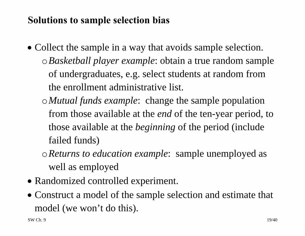
Solutions to sample selection bias

Collect the sample in a way that avoids sample selection. o Basketball player example: obtain a true random sample

of undergraduates, e.g. select students at random from the enrollment administrative list.

o Mutual funds example: change the sample population from those available at the end of the ten-year period, to those available at the beginning of the period (include failed funds)

o Returns to education example: sample unemployed as well as employed

Randomized controlled experiment. Construct a model of the sample selection and estimate that

model (we won’t do this).

SW Ch. 9 20/40

5. Simultaneous causality bias So far we have assumed that X causes Y. What if Y causes X, too? Example: Class size effect Low STR results in better test scores But suppose districts with low test scores are given extra

resources: as a result of a political process they also have low STR

What does this mean for a regression of TestScore on STR?

SW Ch. 9 21/40

Simultaneous causality bias in equations (a) Causal effect on Y of X: Yi = 0 + 1Xi + ui (b) Causal effect on X of Y: Xi = 0 + 1Yi + vi Large ui means large Yi, which implies large Xi (if 1>0)

Thus corr(Xi,ui) 0

Thus 1̂ is biased and inconsistent.

SW Ch. 9 22/40

Solutions to simultaneous causality bias

1. Run a randomized controlled experiment. Because Xi is chosen at random by the experimenter, there is no feedback from the outcome variable to Yi (assuming perfect compliance).

2. Develop and estimate a complete model of bi-directional

causality. This is difficult in practice. ---------------------------------

3. Use instrumental variables regression to estimate the causal effect of interest (effect of X on Y, ignoring effect of Y on X).

SW Ch. 9 23/40

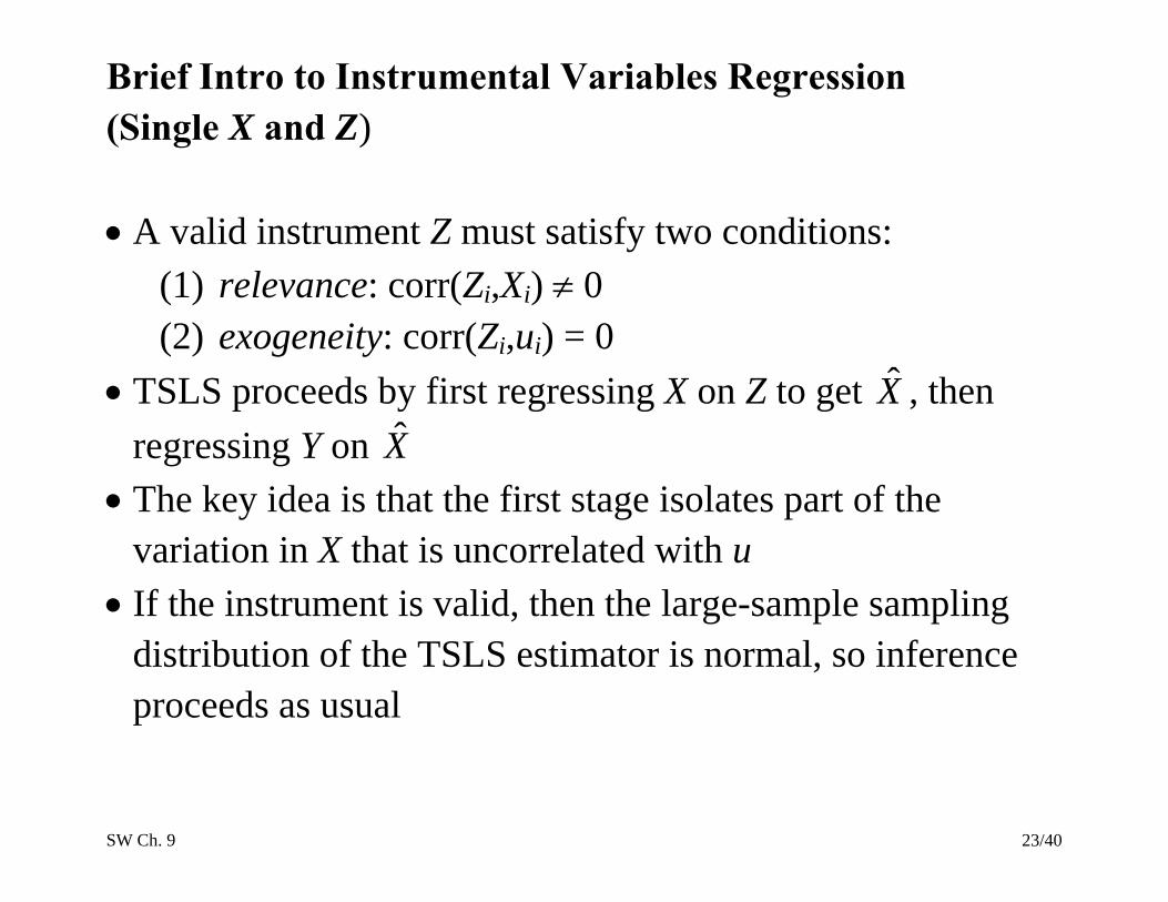
Brief Intro to Instrumental Variables Regression (Single X and Z) A valid instrument Z must satisfy two conditions:

(1) relevance: corr(Zi,Xi) 0 (2) exogeneity: corr(Zi,ui) = 0

TSLS proceeds by first regressing X on Z to get X̂ , then regressing Y on X̂

The key idea is that the first stage isolates part of the variation in X that is uncorrelated with u

If the instrument is valid, then the large-sample sampling distribution of the TSLS estimator is normal, so inference proceeds as usual

SW Ch. 9 24/40

IV Regression: Test scores and class size The California test score/class size regressions still could

have OV bias (e.g. parental involvement). In principle, this bias can be eliminated by IV regression

(TSLS). IV regression requires a valid instrument, that is, an

instrument that is: (1) relevant: corr(Zi,STRi) 0 (2) exogenous: corr(Zi,ui) = 0

SW Ch. 9 25/40

IV Regression: Test scores and class size, ctd. Here is a (hypothetical) instrument: some districts, randomly hit by an earthquake, “double up”

classrooms: Zi = Quakei = 1 if hit by quake, = 0 otherwise

Do the two conditions for a valid instrument hold? The earthquake makes it as if the districts were in a random

assignment experiment. Thus, the variation in STR arising from the earthquake is exogenous.

The first stage of TSLS regresses STR against Quake, thereby isolating the part of STR that is exogenous (the part that is “as if” randomly assigned)

SW Ch. 9 26/40

Applying External and Internal Validity: Test Scores and Class Size

Objective: Assess the threats to the internal and external validity of the empirical analysis of the California test score data. External validity

o Compare results for California and Massachusetts o Think hard…

Internal validity o Go through the list of five potential threats to internal

validity and think hard…

SW Ch. 9 27/40

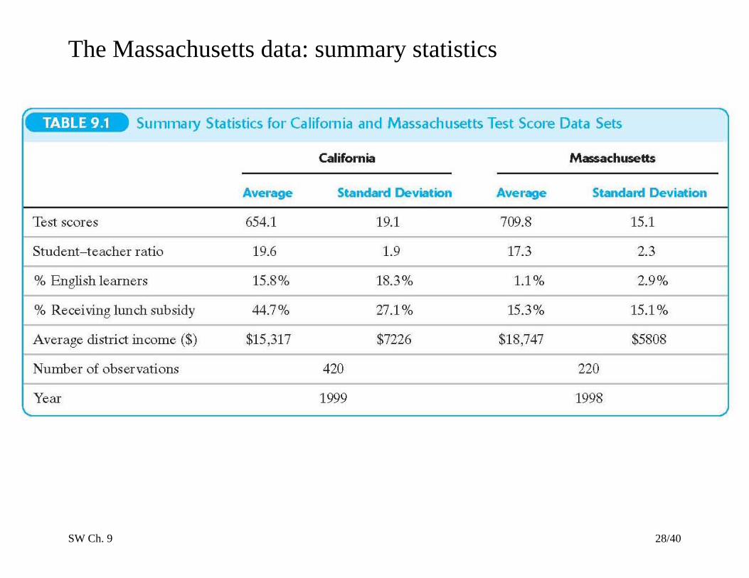
Check of external validity We will compare the California study to one using Massachusetts data

The Massachusetts data set 220 elementary school districts Test: 1998 MCAS test – fourth grade total (Math +

English + Science) Variables: STR, TestScore, PctEL, LunchPct, Income

SW Ch. 9 28/40

The Massachusetts data: summary statistics

SW Ch. 9 29/40

Test scores vs. Income & regression lines: Massachusetts data

SW Ch. 9 30/40

SW Ch. 9 31/40

How do the Mass and California results compare? Logarithmic v. cubic function for STR? Evidence of nonlinearity in TestScore-STR relation? Is there a significant HiELSTR interaction?

SW Ch. 9 32/40

Predicted effects for a class size reduction of 2 Linear specification for Mass:

TestScore = 744.0 – 0.64STR – 0.437PctEL – 0.582LunchPct (21.3) (0.27) (0.303) (0.097)

– 3.07Income + 0.164Income2 – 0.0022Income3 (2.35) (0.085) (0.0010) Estimated effect = -0.64(-2) = 1.28

SW Ch. 9 33/40

Computing predicted effects in nonlinear models

TestScore = 655.5 + 12.4STR – 0.680STR2 + 0.0115STR3

– 0.434PctEL – 0.587LunchPct – 3.48Income + 0.174Income2 – 0.0023Income3

Estimated reduction from 20 students to 18:

TestScore = [12.420 – 0.680202 + 0.0115203] – [12.418 – 0.680182 + 0.0115183] = 1.98

compare with estimate from linear model of 1.28

SW Ch. 9 34/40

Summary of Findings for Massachusetts

Coefficient on STR falls from –1.72 to –0.69 when control

variables for student and district characteristics are included – an indication that the original estimate contained omitted variable bias.

The class size effect is statistically significant at the 1% significance level, after controlling for student and district characteristics

No statistical evidence of nonlinearities in the TestScore – STR relation

No statistical evidence of STR – PctEL interaction

SW Ch. 9 35/40

Comparison of estimated class size effects: CA vs. MA

SW Ch. 9 36/40

Summary: Comparison of California and Massachusetts Regression Analyses

Class size effect falls in both CA, MA data when student

and district control variables are added. Class size effect is statistically significant in both CA, MA

data. Estimated effect of a 2-student reduction in STR is

quantitatively similar for CA, MA. Neither data set shows evidence of STR – PctEL interaction. Some evidence of STR nonlinearities in CA data, but not in

MA data.

SW Ch. 9 37/40

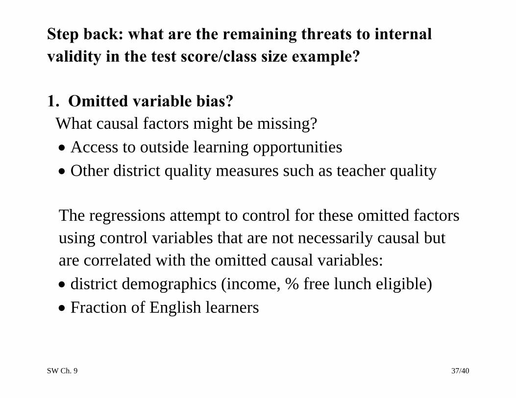
Step back: what are the remaining threats to internal validity in the test score/class size example? 1. Omitted variable bias? What causal factors might be missing? Access to outside learning opportunities Other district quality measures such as teacher quality The regressions attempt to control for these omitted factors using control variables that are not necessarily causal but are correlated with the omitted causal variables: district demographics (income, % free lunch eligible) Fraction of English learners

SW Ch. 9 38/40

Omitted variable bias, ctd. Are the control variables effective? That is, after including the control variables, is the error term uncorrelated with STR? Answering this requires using judgment. There is some evidence that the control variables are

effective: o The STR coefficient doesn’t change much when the

control variables specifications change o The results for California and Massachusetts are

similar – so if there is OV bias remaining, that OV bias would need to be similar in the two data sets

SW Ch. 9 39/40

2. Wrong functional form? We have tried quite a few different functional forms, in

both the California and Mass. data Nonlinear effects are modest Plausibly, this is not a major threat at this point.

3. Errors-in-variables bias? The data are administrative so it’s unlikely that there are

substantial reporting/typo type errors. STR is a district-wide measure, so students who take the

test might not have experienced the measured STR for the district – a complicated type of measurement error

Ideally we would like data on individual students, by grade level.

SW Ch. 9 40/40

4. Sample selection bias? Sample is all elementary public school districts (in

California and in Mass.) – there are no missing data No reason to think that selection is a problem if we are

interested only in public school students. 5. Simultaneous causality bias? School funding equalization based on test scores could

cause simultaneous causality. This was not in place in California or Mass. during these

samples, so simultaneous causality bias is arguably not important.