Assessing Relationships between Stream Water … Relationships between Stream Water Quality and ... Schematic representation of the hydrologic cycle .....21 Figure 9: The Nitrogen

Assessing Relationships between Stream Water Quality and

Watershed Attributes Using the SWAT2000 Integrated Watershed

Model A Case Study in the Rönne River Basin,

Sweden

Assefa Kumssa Afeta March, 2006

Assessing Relationships between Stream Water Quality and Watershed

Attributes Using the SWAT2000 Integrated Watershed Model

A Case Study in the Rönne River Basin, Sweden

by

Assefa Kumssa Afeta Thesis submitted to the International Institute for Geo-information Science and Earth Observation in partial fulfilment of the requirements for the degree of Master of Science in Geo-information Science and Earth Observation, Specialisation: Environmental Modelling and Management Thesis Assessment Board Chairman: Prof. Dr. A.K. Skidmore (NRS, ITC) External Examiner: Dr. M. S. Krol (WEM, University of Twente) Supervisor: Dr. Ir. C.M.M. Mannaerts (WRS, ITC) Course Coordinator: M.sc A. Kooiman (ITC)

International Institute for Geo-information Science and Earth Observation, Enschede, The Netherlands

Disclaimer

This document describes work undertaken as part of a programme of study at the International Institute for Geo-information Science and Earth Observation. All views and opinions expressed therein remain the sole responsibility of the author, and do not necessarily represent those of the institute.

i

Abstract

An integrated spatial modelling approach was used to assess the relationships between watershed attributes and diffuse nitrate loading within the Rönne River basin in Southern Sweden. The soil and water assessment tool (SWAT2000) interfaced with Arc View GIS was used to extract and process input parameters from various GIS data layers including digital elevation model, land cover and soil maps for the SWAT2000 model. The model was calibrated and then validated for stream flow at two locations and for nitrate concentration in stream water at one location within the basin. Several input parameters of the SWAT model were adjusted during calibration of which runoff curve number (CN), soil available water capacity (SOL_AWC), soil evaporation coefficient (ESCO) and nitrate percolation coefficient (NPERCO) were found to be most sensitive. The Nash-Sutcliffe prediction efficiency (ENS), coefficient of determination (r2) and graphical depictions were used to evaluate the performance of the model. During the yearly time step, ENS values for the simulations of flow range between 0.65 and 0.78 for both calibration and validation, while values ranging between 0.70 and 0.79 were achieved for r2, suggesting that the model was able to adequately predict stream flows. However, the result obtained for nitrate calibration on the monthly time step was rather poor with negative ENS value, may be due to insufficiency of information on nutrient related processes within the calibration sub-basin. The calibrated model for hydrological conditions was then used to assess nitrate loading in relation to various watershed attributes. The result revealed that nitrate loading by surface water is strongly positively correlated to the percentage area occupied by agricultural land (r=0.9), suggesting 79% of variation in diffuse nitrate emission can be explained by variation in agricultural land cover. On the contrary, nitrate loading is found to be negatively correlated with the area occupied by forest (r=-0.7). Finally, this study showed that SWAT model is a powerful tool that could be used for hydrological analysis of Rönne River basin, especially when dealing with water balance and quantity aspects. However, further nutrient data verification is essential for a reliable estimation of nitrate load values, related to water quality problems, to help effective management planning and decision-making processes within the watershed.

ii

Acknowledgements

First and foremost, my special gratitude goes to the Erasmus Mundus fellowship Programme for facilitating my studies at the University of Southampton in the United Kingdom, Lund University in Sweden and ITC in The Netherlands. The three coordinators of the programme in the three respective institutions: Prof. Dr. A. Skidmore of ITC, Prof. P. Pilesjö of Lund University and Prof. P. M. Atkinson of the University of Southampton deserve my special thanks for their unreserved guidance, close friendliness and making life easier through out my stay in Europe. I am especially grateful to my primary supervisor Prof. Pilesjö for his critical comments and contributions during my thesis work and for facilitating my stay in Sweden during field data collection. The staffs of GIS centre of Lund University, especially Ulrik Mårtensson, Jean-Nicolas Poussart and Dr. Andreas Persson also deserve my sincere appreciation for enthusiastically assisting me in many aspects during my research work. Without their contribution and help, my task would have been difficult. The contribution of my second supervisor Prof. Katarzyna Dabrowska of University of Warsaw in Poland was also notable during the proposal writing stage that I would like to thank her for her encouragement. I would also like to extend my sincere appreciation to SMHI-VASTRA for allowing me to use their data, and Jorgen Rosberg of SMHI for organising and forwarding me the dataset. I am most indebted in many ways to my ITC advisor Dr. Ir. C.M.M. Mannaerts of the Water Resources Department who spared me much of his precious time and provided me with useful guidance from the very beginning of title selection to the final thesis preparation during the course of my research work. His comments were very constructive throughout, and above all I found him to be very friendly and comfortable person to work with. Thank you once again Chris! I would also like to thank the many people who indirectly have helped me with my study. I am especially grateful to Kasech Taddesse and Fanta Terefe for handling all my personal affairs back home in my absence, and above all for offering me a relentless encouragement during the period of my study. Especially, Kasu is truly a wonderful sister of mine for her care and concern have always been enormous and special to me. My cherished friends Siddisee Amanuel and Yodit Teferi also deserve my sincere gratitude for the concern and moral support they offered me. MAY ‘WAAQAA’ BLESS THEM All! Finally, I would like to express my humble appreciation to my friends Alemu Nebebe, Aster Denekew, Habtamu Mulatu, Sabit Yasin and many others for being part of a “family” away from home. I enjoyed the good times we shared together. I also thank my course mates Lillian, Laura, Apichart and Dan for their friendship during our stay.

iii

Table of Contents

Abstract ................................................................................... i Acknowledgements ....................................................................ii Table of Contents ..................................................................... iii List of figures ........................................................................... v List of tables ........................................................................... vii Acronyms .............................................................................. viii 1. Introduction ....................................................................... 1

1.1 Background and Problem Statement............................... 1 1.2 Objectives .................................................................. 6 1.3 Research Questions ..................................................... 7 1.4 Hypotheses................................................................. 7 1.5 Research Approach ...................................................... 8

2 An Integrated Spatial Approach for Watershed Management: Overview of Tools ............................................................... 9

2.1 General...................................................................... 9 2.2 Hydrologic and Water Quality Models.............................. 9 2.3 The Role of Remote Sensing Data .................................13 2.4 The Role of Geographic Information System ...................14

3 Methods and Materials ........................................................15 3.1 Description of the Study Area.......................................16 3.2 Description of the SWAT2000 Model ..............................20

3.2.1 Hydrology ..............................................................21 3.2.2 Erosion/sedimentation .............................................24 3.2.3 Nutrients................................................................24

3.3 Model Inputs..............................................................30 3.3.1 Watershed Delineation .............................................30 3.3.2 Land Use and Soil Characterization ............................32 3.3.3 Climate Data ..........................................................40 3.3.4 Management Practice...............................................41

3.4 Model Calibration and Validation ...................................42 4 Results .............................................................................47

4.1 Calibration.................................................................47 4.1.1 Stream Flow ...........................................................47 4.1.2 Nutrient (NO3-N) .....................................................52

4.2 Validation ..................................................................53 4.3 Modelling Nutrient (NO3) Loading of the Rönne Basin .......58

4.3.1 NO3 Diffuse Emission Predicting Variables ...................58 4.3.2 NO3 Concentration in Stream Water: Spatial Variation ..61 4.3.3 NO3 Loadings under two Management Scenarios ..........62

5 Discussion.........................................................................65 5.1 Stream Water Flow Modelling .......................................65

iv

5.2 Nutrient (NO3) Load Modelling ......................................67 5.3 Scenario Analysis .......................................................69

6 Conclusion ........................................................................73 References .............................................................................75 Appendices .............................................................................81

Appendix 1: Topographic statistical summary............................81 A-1.1 Elevation report for the watershed ...............................81 A-1.2 Elevation report for each sub-basin ..............................81

Appendix 2: Landsat image and classified land use map .............83 Appendix 3: SWAT main output files ........................................84 Appendix 4: Calibration and validation data ..............................84

A-4.1: Flow calibration data.................................................84 A-4.2: Flow validation data..................................................87 A-4.3: NO3 Calibration data .................................................90

Appendix 5: Different land use proportions vs. Nsurq .................92 Appendix 6: Annual Basin Values: Water balance and nutrient.....93

v

List of figures

Figure 1: Annual average nitrate concentrations (μg N/l) in different sized European rivers........................................................... 4

Figure 2: Conceptual framework of the research work.................... 8 Figure 3: Schematic Diagram of the Integrated Modelling Approach 15 Figure 4: Location of Rönne River basin in Southern Sweden..........16 Figure 5: A Panoramatic view of Rönne River ..............................17 Figure 6: Granite/gneiss rock outcrops .......................................18 Figure 7: Lake Ringsjön and the surrounding cultivated land ..........19 Figure 8: Schematic representation of the hydrologic cycle ...........21 Figure 9: The Nitrogen Cycle ....................................................25 Figure 10: SWAT soil nitrogen pools and processes ......................25 Figure 11: SWAT soil phosphorus pools and processes .................28 Figure 12: DEM and the delineated watershed/sub-basins .............32 Figure 13: Generalised land use map used as model input .............36 Figure 14: A generalised map of soil types used as model input......38 Figure 15: Model calibration and validation sites ..........................43 Figure 16: Comparison between measured and simulated annual

average stream flow at Ringsjön for model calibration .............47 Figure 17: Comparison between measured and simulated annual

average stream flow at Klippan for model calibration...............48 Figure 18: Measured against simulated monthly average stream flow

at Ringsjön for model calibration ..........................................49 Figure 19: Measured against simulated monthly average stream flow

at Klippan for model calibration ............................................50 Figure 20: Regression and 1:1 line fit plot of observed versus

simulated monthly stream flow at Ringsjön ............................50 Figure 21: Regression and 1:1 line fit plot of observed versus

simulated monthly stream flow at Klippan..............................51 Figure 22: Observed against simulated NO3-N concentration in stream

water at Klippan.................................................................52 Figure 23: Measured monthly average flow (m3/s) vs. NO3

concentration (mg/l) at the outlet of Klippan sub-basin............53 Figure 24: Simulated versus measured annual stream flow at

Ringsjön for model validation ...............................................54 Figure 25: Simulated versus measured annual stream flow at Klippan

for model validation............................................................54 Figure 26: Simulated against measured monthly flow at Ringsjön for

model validation ................................................................55 Figure 27: Simulated against measured monthly flow at Klippan for

model validation ................................................................56 Figure 28: Regression and 1:1 line fit plot of observed versus

simulated monthly flow for model validation at Ringsjön ..........56

vi

Figure 29: Regression and 1:1 line fit plot of observed versus simulated monthly flow for model validation at Klippan............57

Figure 30: Comparison of proportion of agricultural land cover against annual average NO3 loading in surface water .........................60

Figure 31: Comparison of proportion of forest cover against annual average NO3 loading in surface water ...................................60

Figure 32: NO3-N concentration in stream water at different locations along the Rönne River.........................................................61

Figure 33: NO3 loading by surface runoff from different sub-basins, 10-years average (1991-2000) for scenario 1.........................63

Figure 34: NO3 loading by surface runoff from different sub-basins, 10-years average (1991-2000) for scenario 2.........................63

vii

List of tables

Table 1: Summary of watershed-scale continuous hydrologic and non-point source pollution models ........................................11

Table 2: Characteristics of hydrologic soil groups .........................23 Table 3: Curve Number adjustments from Antecedent Moisture

Conditions I, II, III .............................................................23 Table 4: CORINE land cover nomenclature ..................................34 Table 5: Proportion and description of the newly classified land use

types from CORINE ............................................................35 Table 6: Common soil types of the Rönne watershed ....................37 Table 7: Proportion and description of the classified soil types .......39 Table 8: Estimated soil parameters for main soil textures .............39 Table 9: Total nitrogen pressure from agriculture, air deposition and

biological fixation for South Sweden......................................41 Table 10: Schedule of tillage, planting, fertilizer application and

harvesting for model runs....................................................42 Table 11: Initial and final values of SWAT calibration parameters for

stream flow .......................................................................44 Table 12: Summary of calibration results for annual stream flows

(m3/s) at Ringsjön and Klippan.............................................48 Table 13: Summary of calibration results for monthly stream flows at

Ringsjön and Klippan ..........................................................51 Table 14: Summary of validation results for annual flows (m3/s) ....55 Table 15: Summary of validation results for monthly flows ............57 Table 16: Correlation coefficient between NO3 loading (NSURQ - kg

N/ha) and %age field..........................................................59 Table 17: Longitudinal NO3 concentration (mg/l) in stream water

along the main channel of Rönne River..................................61 Table 18: Summary of average annual basin values (1991-2000)

under two management scenarios ........................................62

viii

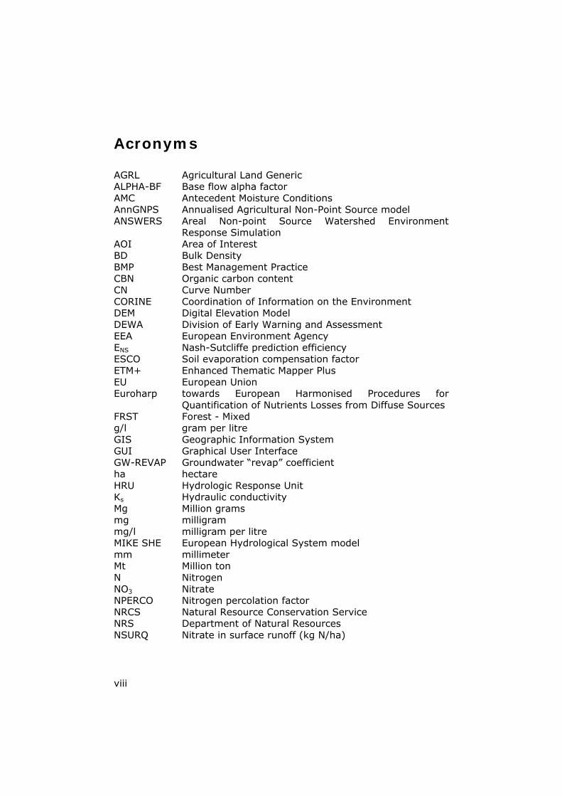
Acronyms

AGRL Agricultural Land Generic ALPHA-BF Base flow alpha factor AMC Antecedent Moisture Conditions AnnGNPS Annualised Agricultural Non-Point Source model ANSWERS Areal Non-point Source Watershed Environment

Response Simulation AOI Area of Interest BD Bulk Density BMP Best Management Practice CBN Organic carbon content CN Curve Number CORINE Coordination of Information on the Environment DEM Digital Elevation Model DEWA Division of Early Warning and Assessment EEA European Environment Agency ENS Nash-Sutcliffe prediction efficiency ESCO Soil evaporation compensation factor ETM+ Enhanced Thematic Mapper Plus EU European Union Euroharp towards European Harmonised Procedures for

Quantification of Nutrients Losses from Diffuse Sources FRST Forest - Mixed g/l gram per litre GIS Geographic Information System GUI Graphical User Interface GW-REVAP Groundwater “revap” coefficient ha hectare HRU Hydrologic Response Unit Ks Hydraulic conductivity Mg Million grams mg milligram mg/l milligram per litre MIKE SHE European Hydrological System model mm millimeter Mt Million ton N Nitrogen NO3 Nitrate NPERCO Nitrogen percolation factor NRCS Natural Resource Conservation Service NRS Department of Natural Resources NSURQ Nitrate in surface runoff (kg N/ha)

ix

P Phosphorous PAST Pasture RIZA Inst. for Inland Water Mgt. & Waste Water Treatment RNGB Range - brush SCS-CN Soil Conservation Service – Curve Number SGU Geological Survey of Sweden SMHI Swedish Meteorological and Hydrological Institute SOL-AWC Soil Water Available Capacity STOWA Foundation for Applied Water Research SWAT Soil and Water Assessment Tool UNEP United Nations Environment Programme URML Residential – Med/low density USDA-ARS United States Department of Agriculture – Agriculture

Research Service USLE Universal Soil Loss Equation VASTRA Swedish Water Management Research Programme WATR Water WEM Department of Water Engineering & Management WETL Wetlands – Mixed WRS Department of Water Resources WWTP Waste Water Treatment Plant

1. Introduction

1.1 Background and Problem Statement

Water, an essential component of the Earth’s ecosystem, is a precious natural resource necessary to maintain human populations and ecosystems that any threat to the sustainability of this resource certainly deserves focused attention. However, freshwaters have been subjected to increasing pressures and suffered quality degradations in the past in many parts of the world (European Commission, 2003; Santhi et al., 2005) despite the continuous renewal of the resources by natural processes of the hydrologic cycle (UNEP/DEWA-Europe, 2004). “Although we as humans recognize this fact, we disregard it by polluting our rivers, lakes, and oceans. Subsequently, we are slowly but surely harming our planet to the point where organisms are dying at a very alarming rate. In addition to innocent organisms dying off, our drinking water has become greatly affected as is our ability to use water for recreational purposes. In order to combat water pollution, we must understand the problems and become part of the solution.”(Krantz and Kifferstein, 2005) Freshwaters, depending on the purpose of demand, have a certain limit of chemical concentrations suitable for aquatic life and human uses (Chapman, 1996). However, high contents of nutrients in water such as nitrates and phosphorus are the major issues in terms of water quality, which have received most attention worldwide (McDonald and Kay, 1988). Most importantly, excess nitrate and phosphorus concentrations in surface waters such as lakes and coastal waters cause eutrophication, which is considered as a serious environmental problem. Eutrophication over-stimulates the growth of algae resulting in oxygen deficiency that becomes hazardous to the aquatic life through decomposition. High nitrate content in drinking waters can also cause a significant health risk to humans. Excessive nutrients in the ecosystem are mainly caused by anthropogenic activities such as runoff from industrial, urban and agricultural lands. Additional sources such as direct atmospheric deposition (De Wit, 1999), landscape morphology, hydrological conditions, biogeochemical processes in soil, sediment and geological characteristics have also contributions but less significantly. There has been, however, a general understanding that agricultural sources

Introduction

2

due to the increased use of manures and manufactured inorganic fertilizers in global agriculture are the single greatest causes of pollution degrading the quality of surface waters as described by several researchers of the field (Bhuyan et al., 2003; Chapman, 1996; De Wit, 1999; Jonsson et al., 2002; Matejicek et al., 2003; Santhi et al., 2005; Van Herpe and De Troch, 2000). The rate of use of nitrogen fertilizer, for example, has increased steadily from the 1950s until the late 1980s coinciding with the end of World War II and the collapse of the former Soviet Union respectively. The disintegration of the Soviet Union led to great disruptions in agriculture and fertilizer use for a short period of time (Matson et al., 1997), but has shown a rapid growing trend since 1995 again with much of the demand driven by an increased use in China. The annual global nitrogen fertilizer consumption has increased from 10Mt in 1960s to nearly 90Mt in late 1990s (Matson et al., 1997). Such human activity with increased reliance on manufactured inorganic fertilizers and the rate of change in the pattern of use has caused significant effect (Galloway, 1998; Vitousek et al., 1997) on the global cycling of nitrogen, especially on the movement of nutrients to estuaries and other coastal waters. When inorganic fertilizer is applied to a field, it can move through a variety of flow paths to downstream aquatic ecosystems. Some of the fertilizer leaches directly to groundwater and surface waters, with the range varying from 3 percent to 80 percent of the fertilizer applied, depending upon soil characteristics, climate, and crop type (Howarth, 1996). The amount of global phosphorus flux, for example, carried in eroded materials and wastewater from the land to the seas was estimated at 22 Mt P yr-1 (Howarth, 1996), which to have been estimated at about 8 Mt P yr-1 prior to increased human agricultural and industrial activity. The trend in Europe is not significantly different per se from the global trend in terms of fertilizer use and hence water quality problems associated with such agricultural activities. Although point sources such as sewage discharges may contribute significantly to nutrient enrichment in some regions of the continent, diffuse sources, particularly agriculture, are still the major contributors (UNEP/DEWA-Europe, 2004). The greater intensification of agriculture and higher productivity during the past 50 years has resulted in a significant increase in fertilizer use, particularly organic nitrogen use (European Commission, 2002; Wolf et al., 2003). According to European Commission report, mineral nitrogen consumption in EU which was less than 1Mt in 1945 has considerably risen to a peak of over 11Mt in 1985 (European Commission, 2002). Similarly, intensive animal

Chapter 1

3

husbandry increased during the same period, contributing to a greater overall nitrogen load through manure. Nitrogen “pressure” from animal husbandry such as cows, pigs, poultry, and sheep on agricultural soils is approximately 8Mt per year based on 1997 data (European Commission, 2002). The greater density of livestock population and manure applications has resulted not only in the direct deposition of nutrients into the ecosystem but also produced a strong volatilization of ammonia to the atmosphere and deposition back on soils and waters with values up to 50-60 kg N/ha/yr. Categorically, about 50% of the nearly 20Mt annual N input to EU agricultural soils comes from mineral fertilizer while the remaining 50% is attributed to air deposition, biological fixation and livestock manure spreading. According to the European Commission report (2002), the intensified agricultural activity has also resulted in the reduction of permanent grassland and disappearance of wetland areas, which could serve as buffer and sink zones for nutrients. This has subsequently caused increased erosion, high rate of run-off and more rapid flow of nutrients to the aquatic ecosystem and groundwater (European Commission, 2002), with the most important consequences of surface water eutrophication and possible health effects. The increasing concentration of nitrate in drinking water and eutrophication of surface waters with adverse environmental and health effects triggered growing public concern, which has prompted the European Union for action to improve water quality since the 1970s. During the last two decades, new agricultural policies and environmental regulations have been enforced in many European countries with the objective of reducing agricultural diffuse source pollution, improve water quality and protect the aquatic habitat from eutrophication (Grizzetti et al., 2003). Limits have been established to agricultural fertilizer inputs in order to control water pollution caused by nitrates from agricultural sources through the nitrate directive issued in 1991 (European Community, 1991). A similar directive was issued concerning urban waste water treatment in the same year to tackle the problem of nitrate pollution. The same nitrate problem has also been addressed in the water framework directives of 2000, with the motto of “getting Europe’s water cleaner”, that has to get polluted waters clean again, and ensure clean waters are kept clean. This includes nitrate under the surveillance monitoring list, mainly aimed at controlling and reducing water pollution resulting from discharge of livestock effluents and the excessive use of fertilizers on agricultural land (European Commission, 2000). The directive, generally, emphasizes on agricultural pollution sources in a watershed and provides a basis for taking actions needed to restore a

Introduction

4

water body thus the respective member countries are required to act and implement accordingly. The efforts made so far have shown significant progress in controlling point sources from sewage and industrial wastes resulting in lower levels of most pollutants such as phosphorus (EEA, 1998a). However, despite the EU Nitrate Directives and the increased use of agri-environmental measures, the agricultural sector remains the main source of diffuse pollutants without as much progress. Nitrogen surpluses from agriculture are rather constant and hence levels in rivers are still as high as they were in the early 1990s (EEA, 2001; EEA, 2003; European Commission, 2003) as indicated in figure 1.

Figure 1: Annual average nitrate concentrations (μg N/l) in different sized European rivers

In Sweden, similar to most EU countries, the load of nutrients on streams, lakes and coastal waters has increased dramatically after World War II mainly due to the intensification of agricultural activities (Arheimer et al., 2004; Ekologgruppen, 2000). This has caused the reduction of wetland areas by 90% thereby stimulating the growth of eutrophication in surface waters and reduction of biological diversity. Nitrogen input to agricultural soils from livestock manure was estimated between 40 to 50 kg N/ha/yr in 1997, while the total nitrogen pressure including mineral fertilizer use, livestock manure spreading, atmospheric deposition and biological fixation was between 100-125 kg N/ha/yr (European Commission, 2002). Average nitrogen atmospheric deposition in Southern Sweden, including the study area, has been estimated between 5 and 10kg N/ha/yr. In view of the EU water policy, the Swedish Government has put in place policy measures and has been implementing several conservation practices aimed at reducing anthropogenic nitrogen

Chapter 1

5

emissions, mainly due to uncontrolled municipal sewage systems and agricultural practices (Ekologgruppen, 2000) by regulating urban waste disposal systems, the use of excessive fertilizers and handling of manures. In addition to policy enforcements to improve urban sewage systems and changing agricultural practices, complimentary measures to reduce nutrient transport to inland and coastal waters are also being undertaken to improve water quality. These include the creation of wetlands, ponds and buffer-zones in the intensively cultivated areas, to increase nutrient sink areas. But the achievement is rather small (Arheimer et al., 2004) to attain the desired target and eutrophication is still a subject of major concern in many Swedish inland and coastal waters, particularly in the intensively farmed plain lands, which are more common in central and southern part of the country. Although there have been improvements, the level of phosphorus content in several lakes is still high that they can be considered eutrophic. Sources indicate that the concentration of nitrate, especially in groundwater, is even worse showing rather an increasing trend (European Commission, 2002), and “water quality problems still remain due to diffuse leaching from arable land and from sediment loading”(Arheimer et al., 2004). The proposed research area, the Rönne River basin, is the second largest catchment in Skåne, southern Sweden, known to have been suffering from such elevated nutrient loadings and subsequent eutrophication of surface waters within the watershed (Arheimer et al., 2004). The problem has been persistent that raised a growing concern, due to: firstly, its socioeconomic and ecological importance in that it contains lakes such as Ringsjön, which is frequently affected by algal blooms. In addition to being a habitat for aquatic ecosystem, Lake Ringsjön is currently used as a spare drinking water source for people inhabiting the area. Secondly, the catchment drains through the Rönne River to the coastal water of the North Sea. Coastal waters, in general, are ecologically sensitive from inland pollution sources and in particular the coastal water of the North Sea is a subject of major concern in the EU that led the current study area to have been designated as “nitrate vulnerable zone”. As a result, the Rönne river basin has been used as a pilot catchment area for eutrophication control (Arheimer et al., 2004) using an integrated river basin management approach. Effective decision-making processes for best management options such as the implementation of EU water framework directives require relatively reliable, not expensive and timely information. Conventional monitoring methods like field stream water quality data collection and analysis as a decision-making tool is expensive, time consuming

Introduction

6

(Santhi et al., 2005) and even it becomes more complex and difficult especially when dealing with large watersheds such as Rönne river basin characterised by mixed land use, soil types, topography and geological conditions. It is believed that a watershed based modelling approach, with spatial or geographic information system capability, allows for the consideration of such attribute variations, and quantification of the impacts at different spatial and temporal scales. The application of watershed models as decision support tools in reducing nutrient leaching from different land use areas in a watershed and the resulting adverse environmental effects in general and water quality in particular has been discussed in several researched works (Arheimer et al., 2004; Arnold et al., 1998; Bhuyan et al., 2003; Borah and Bera, 2003; Grizzetti et al., 2003; Jayakrishnan et al., 2005; Jha et al., 2004; Jonsson et al., 2002; Santhi et al., 2005; Tolson and Shoemaker, 2004; Tripathi et al., 2003; White et al., 1992; Wolf et al., 2003) Hence, this study is intending to apply an integrated modelling approach that uses remote sensing data, geographic information system and a physically based simulation model in order to relate nutrient loadings with watershed attributes. Previous scientific effort made, in this regard, in the study area is that of the VASTRA project - The Swedish Water Management Research Programme - which has been focusing on the development and demonstration of models for more efficient eutrophication control. It is believed that this study will contribute towards such efforts, in particular, and the implementation of the EU water framework directive, in general, by identifying the main source and sink areas of nutrients responsible for adverse environmental impacts such as eutrophication and health risks within the Rönne River basin and the North Sea coastal waters.

1.2 Objectives

In light of the above background and problem statement, the proposed research project has the following general and specific objectives: General Objective: • To analyze and explain the spatial relationships between nutrient

fluxes (NO3-N loadings) of the Rönne river basin and (sub-) watershed area source/sink attributes using remote sensing data, spatial GIS analyses and the Soil and Water Assessment Tool (SWAT2000 model).

Chapter 1

7

Specific objectives: • To simulate the hydrologic flow regime and nutrient (NO3) loading

at selected sub-basin outlets from the different (sub-)watershed area attributes;

• To assess the spatial relationship between watershed attributes and NO3 as a source/sink effect, and hence the contribution of agricultural land as compared to others;

• To test the accuracy of the modelling process against measured/observed stream flow and nutrient loading data;

1.3 Research Questions

The research will try to address the following questions: • Is there any spatial relationship between stream water quality

(NO3 loading) and watershed characteristics of the Rönne River basin? If so, which of the watershed attributes, for example land use, soil types, topographic features, etc, are the most explanatory variables or predictors?

• Which sources, i.e. agricultural land, forest, etc, contribute most to NO3 loads in stream water?

• Does change in land use/cover account for changes in stream water quality?

• Can SWAT accurately predict stream flow and nutrient loadings and therefore can probably be used to model similar watersheds?

1.4 Hypotheses

• Agricultural lands are the most contributors of nitrates in stream waters of the Rönne River basin compared to other sources;

• Spatially, the concentration of nitrate increases longitudinally downstream along the Rönne River due to the cumulative effect of the upstream sub-basin characteristics.

• Change in land use scenario would result change in nitrate loading trend and hence stream water quality.

• SWAT predicts about 70% of observed watershed processes, e.g. stream water flow and nitrate loading, within the watershed.

Introduction

8

1.5 Research Approach

A simplified research conceptual framework is indicated in the following flowchart, figure 2.

Figure 2: Conceptual framework of the research work

Chapter 2

9

2 An Integrated Spatial Approach for Watershed Management: Overview

of Tools

2.1 General

The causes of water pollution are generally attributed to diffuse sources originated mainly from agricultural runoff and point sources originated from domestic and industrial effluents. The sources of such pollutants and their routing mechanism are controlled by several natural and anthropogenic factors such as climatic conditions, hydrologic regimes, soil types, land uses, geological and topographical features, etc. Such natural and human-induced complexities make the protection of pollution and hence water resource management too difficult. Therefore, in order to characterize pollutants and their mechanism of movement within the environment, extensive knowledge and information is required not only about the pollutants in concern but also the controlling factors mentioned within the environment at varying spatial and temporal scales. The underlying challenge is, however, difficulties that may exist in understanding and evaluating such natural processes leading to impairments in a watershed (Borah and Bera, 2003). Description of the appropriate spatial and temporal variability of processes based on conventional measurements or observations, for example field sampling and analysis of stream water quality, at selected locations to represent and explain the entire watershed is ineffective, expensive and time consuming increasing the intricacy on effective decision-making process. An integrated spatial approach that combines a watershed scale hydrologic and water quality models, remote sensing and geographic information system (GIS) led to tremendous progress during the last few decades (Jayakrishnan et al., 2005) in alleviating such problems and demonstrated to be useful tool in studying, understanding and quantifying the impact of major land use changes and other related watershed characteristics on both water quality and quantity.

2.2 Hydrologic and Water Quality Models

Hydrologic models are becoming increasingly essential in water management (STOWA/RIZA, 1999) as they are powerful tools in

An Integrated Spatial Approach for Watershed Management: Overview of Tools

10

hydrologic system investigation by representing known or assumed functions mathematically that explains the various components of a hydrologic cycle. Basically, two broad categories of hydrologic models are possible – deterministic and stochastic (STOWA/RIZA, 1999). Stochastic models are fully data or field measurement oriented while deterministic models are based on known physical processes and laws. Deterministic models are the most widely used models and can be further subdivided into whether they are based on a simple empirical relation with spatially lumped description of the watershed or whether they are a physically based and spatially distributed description of the catchment area involving equations with computationally intensive numerical solutions (Borah and Bera, 2003). Empirical models are based on functions relating basin average input data to outputs that may produce reasonable results. However, since they do not have any physical basis, such models are not expected to accurately represent the spatial and temporal details of the watershed properties as desired. Spatially distributed models, on the other hand, are based on human knowledge of the physical process, which are representative of observed hydrologic phenomena that control the response of the watershed with known geographic locations and attributes. The spatially distributed nature of such models allow a multi-purpose assessment of the effect of spatially and temporally variable processes and watershed properties on the hydrological responses (Romanowicz et al., 2005) making these kind of models more attractive for studying land and water management options. However, despite the growing demands, several shortcomings are associated with the use of spatially distributed hydrologic and water quality models in watershed management decision making process due to: firstly, they involve intensive data demand that cannot be easily met in many practical aspects because of unavailability or do not just satisfy the desired quality standards; secondly, they require tedious computational time and advanced computing machines increasing the cost associated with the modelling process; thirdly, they require an in-depth scientific skill and understanding, for example, related to model parameterization schemes (Romanowicz et al., 2005). Therefore, it will be imperative to decide upon an appropriate model for a given watershed application through compromising between cheap but simple models and detailed but computationally intensive and expensive models (Borah and Bera, 2003).

Chapter 2

11

Models can also vary based on their capability of simulating the temporal scale of processes, categorised as short-term single event based and long-term continuous simulation models. Event-based models are designed for analyzing single-event storms and assessing watershed management practices, especially structural practices. Agricultural Non-Point Source Pollution model (AGNPS), Areal Non-point Source Watershed Environment Response Simulation (ANSWERS), Dynamic Watershed Simulation model (DWSM), and KINmatic runoff and EROSion model (KINEROS) are examples of single rainfall event models. Continuous simulation models are, on the other hand, designed for analyzing long-term effects of hydrological changes and watershed management, especially agricultural, practices. Annualized Agricultural Non-Point Source model (AnnAGNPS), ANSWERS-continuous, Hydrological Simulation Program–Fortran (HSPF), and Soil and Water Assessment Tool (SWAT) are examples of continuous models. While detailed descriptions and references for some selected models in both categories were given in Borah and Bera (2003), a summary of four selected models of continuous types, extracted from the same source, are given in table 1 for comparison purposes. The extensive review of the various non-point source pollution models and their applications (Borah and Bera, 2003) indicated that SWAT (Arnold et al., 1998) is suitable for long-term continuous predictions in agricultural watersheds. A more detailed description of SWAT model is given in section 3.2

Table 1: Summary of watershed-scale continuous hydrologic and non-point source pollution models Description/ Criteria

AnnAGNPS ANSWERS-Continuous

MIKE SHE SWAT

Model compon-ents/ capabili-ties

Hydrology, transport of sediment, nutrients, and pesticides resulting from snowmelt, precipitation and irrigation, source accounting capability, and user interactive programs including TOPAGNPS generating cells and stream

Daily water balance, infiltration, runoff and surface water routing, drainage, river routing, ET, sediment detachment, sediment transport, nitrogen and phosphorous transformations, nutrient losses through uptake, runoff, and

Interception -ET, overland and channel flow, unsaturated zone, saturated zone, snowmelt, exchange between aquifer and rivers, advection and dispersion of solutes, geochemical processes, crop growth and nitrogen processes in the

Hydrology, weather, sedimentation, soil temperature, crop growth, nutrients, pesticides, agricultural management, channel and reservoir routing, water transfer, and part of the USEPA BASINS modeling system with user interface and ArcViewGIS platform.


12

network from DEM.

sediment. root zone, soil erosion, dual porosity, irrigation, and user interface with pre- and post-processing, GIS, and UNIRAS for graphical presentation

Tempor-al scale

Long term; daily or sub-daily steps.

Long term; dual time steps: daily for dry days and 30 seconds for days with precipitation.

Long term and storm event; variable steps depending numerical stability.

Long term; daily steps.

Waters-hed represe-ntation

Homogeneous land areas (cells), reaches, and impoundments.

Square grids with uniform hydrologic characteristics, some having companion channel elements; 1-D simulations.

2-D rectangular/square overland grids, 1-D channels, 1-D unsaturated and 3-D saturated flow layers.

Sub-basins grouped based on climate, hydrologic response units (lumped areas with same cover, soil, and management), ponds, groundwater, and main channel.

Rainfall excess on overlan-d/ water balance

Water balance for constant sub-daily time steps and two soil layers (8-in. tillage depth and user supplied second layer).

Daily water balance, rainfall excess using interception, Green- Ampt infiltration equation, and surface storage coefficients.

Interception and ET loss and vertical flow solving Richards’s equation using implicit numerical method.

Daily water budget; precipitation, runoff, ET, percolation, and return flow from subsurface and groundwater flow.

Runoff on overlan-d

Runoff curve number generating daily runoff following SWRRB and EPIC procedures and SCS TR-55 method for peak flow.

Manning and continuity equations (temporarily variable and spatially uniform) solved by explicit numerical scheme.

2-D diffusive wave equations solved by an implicit finite difference scheme.

Runoff volume using curve number and flow peak using modified Rational formula or SCS TR-55 method.

Runoff in channel

Assuming trapezoidal and compound cross -sections, Manning’s equation is numerically solved for hydraulic parameters and

Manning and continuity equations (temporarily variable and spatially uniform) solved by explicit numerical scheme.

1-D diffusive wave equations solved by an implicit finite difference scheme.

Routing based on variable storage coefficient method and flow using Manning’s equation adjusted for transmission losses, evaporation, diversions, and

Chapter 2

13

TR-55 for peak flow.

return flow.

Overlan-d sedime-nt

Uses RUSLE to generate sheet and rill erosion daily or user-defined runoff event, HUSLE for delivery ratio, and sediment deposition based on size distribution and particle fall velocity.

Raindrop detachment using rainfall intensity and USLE factors, flow erosion using unit-width flow and USLE factors, and transport and deposition of sediment sizes using modified Yalin’s equation.

No information. Sediment yield based on Modified Universal Soil Loss Equation (MUSLE) expressed in terms of runoff volume, peak flow, and USLE factors.

Chemic-al simulat-ion

Soil moisture, nutrients, and pesticides in each cell are tracked using NRCS soil databases and crop information, and reach routing includes fate and transport of nitrogen, phosphorous, and individual pesticides, and organic carbon.

Nitrogen and phosphorous transport and transformations through mineralization, ammonification, nitrification, and denitrification, and losses through uptake, runoff, and sediment.

Dissolved conservative solutes in surface, soil, and ground waters by solving numerically the advection dispersion equation for the respective regimes.

Nitrate-N based on water volume and average concentration, runoff P based on partitioning factor, daily organic N and sediment adsorbed P losses using loading functions, crop N and P use from supply and demand, and pesticides based on plant leaf-area -index, application efficiency, wash off fraction, organic carbon adsorption coefficient, and exponential decay according to half lives.

BMP evaluat-ion

Agricultural management.

Impact of watershed management practices on runoff and sediment losses.

No information.

Agricultural management: tillage, irrigation, fertilization, pesticide applications, and grazing.

Source: (Borah and Bera, 2003)

2.3 The Role of Remote Sensing Data

Models for watershed management require spatial information, concerning the watershed area attributes, as an essential input such as land cover/use, soil types, topography, geology, climatic conditions, population, etc, in order to represent the biophysical


14

processes of the watershed so that the outputs are technically and scientifically effective. While collection of such datasets using conventional methods, i.e. ground based sampling is proved to be costly and time consuming, the use of the state-of-art tools such as remote sensing techniques offer a cheaper and quick means (Engman, 2002; Kerle et al., 2004; Matejicek et al., 2003; Muller et al., 1993) of measuring watershed parameters both qualitatively and quantitatively. Satellite remote sensing methods can also offer the opportunity to cover an extensive area of a watershed being investigated at a time and, more importantly, the electronic data handling format enables the readily incorporation of the data into computer based hydrologic models. Moreover, the repetitive coverage of the satellite images enables to monitor the changes taking place within the watershed and their long-term effect on watershed management practices such as expansion of agricultural lands, deforestation, urbanisation, etc, by comparing multi-temporal images of the same spatial distribution. In conclusion, remote sensing methods provide reliable and essential input data (Engman, 2002; Kerle et al., 2004; Matejicek et al., 2003; Muller et al., 1993; Rao and Kumar, 2004), especially land cover maps, for watershed models in a time and cost-effective manner.

2.4 The Role of Geographic Information System

Pertaining to their integrative capabilities, geographic information systems are also powerful and indispensable tools for watershed-scale hydrologic analysis and modelling (Khairy et al., 2000). The information extracted from satellite data, topographical maps and other data sources representing soils, land use/cover, weather, topography, population, etc could be stored in GIS as a database in tabular, vector and raster formats. GIS, then, allows the effective and efficient integration of such spatial and non-spatial data for model inputs as well as the spatial visualization of outputs. Most of the widely used watershed models were developed in the 1970s and 1980s, whereas since the 1990s the main focus of modelling research was targeted at developing user friendly graphical user interfaces (GUI) and linking with geographic information system (GIS) and remote sensing data (Borah and Bera, 2003). Several water quality models have been integrated and coupled with GIS software so far giving the opportunity of improved and effective data management techniques for watershed modelling. The integration of SWAT2000 with ArcView 3.3 (DiLuzio et al., 2002) is one of such examples.

Chapter 3

15

3 Methods and Materials

The modelling process involves a step by step implementation of methods and tools. Basically three main categories can be identified namely: spatial data collection, preparation and analysis. The specific methods and techniques used in this study are schematically represented by the flow chart in figure 3. Most of the spatial GIS data layers in digital format were obtained from various existing sources. GIS Softwares such as Edas & ArcView available at ITC coupled with SWAT2000 were used for data preparation, integration, analysis and presentation. Statistical analyses of the results were performed using Microsoft office excel 2003.

Figure 3: Schematic Diagram of the Integrated Modelling Approach

Methods and Materials

16

3.1 Description of the Study Area

The study area, Rönne River basin, is the second largest catchment located in the county of Skåne, the most southern region of Sweden. The watershed is elongated in the southeast-northwest direction from 55.8ºLat/13.2ºLon at the southern east end to 56.4ºLat/12.0ºLon at the northern west end. Location map of the study area is shown in figure 4.

Figure 4: Location of Rönne River basin in Southern Sweden

Chapter 3

17

The basin covers a catchment area of 1900km2 being drained by the Rönne River in the northwest direction where it finally enters the North Sea near the city of Ängelhom. Figure 5 shows a panoramatic view of the Rönne River as it crosses agricultural fields (left) and enters the North Sea (right).

Figure 5: A Panoramatic view of Rönne River with respect to agricultural lands and The North Sea

Elevation within the watershed ranges between 0 m near the North Sea and 220 m further in the upstream area. The watershed and its surroundings receive an average annual precipitation of 700mm and the mean annual temperature is 7.4ºC. January and February are the coldest months of the year with average temperatures of -0.7ºC while the maximum temperature occurs in July and August having an average temperature record of 16.3ºC. The annual evaporation and surface runoff have been estimated between 450-550 mm and 200-300mm respectively (Gustafsson, 1992) while The annual mean flow at the outlet of the Rönne River is about 25 m3/s (VASTRA, 2005). Geologically, the watershed area is characterized by the oldest rocks of Precambrian gneisses and granites surrounded by a cover of sedimentary deposits of Early Palaeozoic and Mesozoic ages (Norling and Wikman, 1990). The gneisses and granites are, characterised by deep weathering and intensive fractures, frequently exposed on horsts (figure 6), which are tectonic structures known to occur alternating with grabens along NW-SE trending fracture zones (Daniel, 1978). The lower Palaeozoic is represented by Cambrian quartzitic sandstones and Ordovician-Silurian silty shales while the Mesozoic rocks comprise continental and brackish-marine origin of the Upper Triassic sandstones, clays, and shales succeeded by coal-

Rönne River

Agricultural field

North Sea


18

seams, which have been mined for some 200 years (Daniel, 1978; Norling and Wikman, 1990). Sand, silty and clayey deposits form the top of the pre-Quaternary sedimentary succession of the Jurassic age. The Quaternary deposits of the area are mostly characterized by younger soils of glacial/postglacial clays, silts and sands. The Quaternary period marks the time when Sweden and the surrounding seas were completely glaciated. The most common soil is till or moraine, composed of mainly clayey and fine-grained sediments, and covers extensive area at the surface as well as below other deposits (Gustafsson, 1992). The major soil types of the area are shown on a generalised soil map in figure 14.

Figure 6: Granite/gneiss rock outcrops on a relatively raised morphology or horst structures

Due to variations in geology and geomorphology, widely differing landscape elements can be found, ranging from acid and poor forest brooks to eutrophied agricultural ditches (VASTRA, 2005). Forest dominates most part of the watershed to the north (about 47%) whereas agricultural land dominates the southern part (about 27%). The area is generally considered one of the most favourable for agriculture in Sweden due to the highly fertile soils relative to other parts of the country. The remaining land use types are characterized by urban areas, water bodies and small proportions of wetlands. Cities with over 10,000 inhabitants are (VASTRA, 2005): Ängelholm (35570), Klippan (15539), Höör (14113) and Hörby (13761). Water bodies occupy about 3.5% of the watershed, Lake Ringsjön being the biggest located in the south-eastern part of the catchment. Figure 7 shows the position of Lake Ringsjön relative to the surrounding cultivated land, while the generalised land use map of the area is shown in fig 13.

Granite outcrop

Chapter 3

19

Figure 7: Lake Ringsjön and the surrounding cultivated land

The area is relatively densely populated as compared to other parts of Sweden, a total of nearly 100000 people living in the catchment area out of which about 70000 or 70% are residents of urban areas (VASTRA, 2005). The region has a history of elevated nutrient content due to mainly intensified agricultural activity resulting in nutrient leakage. Lake Ringsjön, which is currently serving as a spare drinking water source, has been suffering from such high nutrient loadings and frequently affected by eutrophication. Consequently, construction and creation of wetlands, ponds and buffer zones have been underway to complement improving water quality, reduce nutrient transport and increase biodiversity in intensively cultivated farmland. Previous scientific efforts made in implementing the EU water framework directive, in Sweden in general and in the study area in particular, are that of the VASTRA project (The Swedish Water Management Research Programme) which has been focusing on the development and demonstration of models for more efficient eutrophication control. Models for nitrogen flow were already developed during Phase I of the project, and similar models for phosphorus have been under construction (VASTRA, 2005). The scenarios modelled so far in VASTRA phase I, indicated that changing agricultural practices, among others, are the most effective and least expensive way of reducing nitrogen transport from land to lakes and finally the sea.

Lake Ringsjön

Agricultural fields


20

3.2 Description of the SWAT2000 Model

The watershed scale model, Soil and Water Assessment Tool (SWAT2000) (Arnold et al., 1998), developed by the United States Department of Agriculture–Agriculture Research Service (USDA-ARS), was used in this research. SWAT2000 was selected in this study because of: (1) its semi-distributed nature that simulates spatial details of processes within a watershed, which is the underlying objective of this research work, (2) its availability free of charge that could be downloaded by all interested users from the internet at http://www.brc.tamus.edu/swat with full of its documentation, (3) it provides an easy-to-use graphical-user interface for model set-up and use that has been integrated into ArcView GIS (DiLuzio et al., 2002) so that the user can easily learn and use within few days of practice, and (4) it is one of the nine contemporary methodologies currently used for quantifying diffuse losses of N and P by European research institutes to inform policy makers at national and international levels (Euroharp, 2005). Soil and Water Assessment Tool (SWAT model) is mostly physically based distributed river basin scale model developed with the objective of simulating the long-time effect of land use practices on water quality, sediment and agricultural chemical yields (Arnold et al., 1998; Neitsch et al., 2002) in a watershed with varying soil types, land uses and climatic conditions. An extensive review of various non-point source pollution models and their applications by Borah and Bera (2003) indicated the suitability of SWAT for long-term continuous simulations in agricultural watersheds. The model has the capability of analysing large watersheds and river basins by subdividing the area into homogeneous sub-basins or sub-watersheds (Santhi et al., 2005). Each sub-basin is further discretized into several hydrologic response units (HRUs) that have distinctive land use and soil combinations. The model requires specific information about the topography, land use, soil type and weather conditions of a watershed. Most of the dataset are commonly readily available from government offices thus reducing the cost and time of field data acquisition. The main components of the model comprise hydrology, weather, erosion/sedimentation, soil temperature, crop growth, nutrients, pesticides, and agricultural/land management (Borah and Bera, 2003). A complete description of each component is given in Arnold et al. (1998) and Neitsch et al. (2002). Nevertheless, brief descriptions of the more relevant components to this study are given here.

Chapter 3

21

3.2.1 Hydrology

SWAT is an integrated hydrological model that simulates the hydrological balances of a watershed, which is the driving force behind everything that happens in the watershed (Neitsch et al., 2002) such as precipitation, stream flow, groundwater flow, evapotranspiration, and infiltration. Simulation of the hydrologic cycle by SWAT is divided in to two parts: (1) the land phase of the hydrologic cycle that controls the amount of water, sediment, nutrient and pesticide loadings to the main channel for each sub-basin and (2) the water/routing phase of the hydrologic cycle that controls the movement of water, sediment, nutrients, and pesticides through the channel network of the watershed to the outlet (Neitsch et al., 2002). Figure 8 shows the hydrologic cycle simulated by SWAT2000.

Figure 8: Schematic representation of the hydrologic cycle (after Neitsch et al., 2002)

The land phase of the hydrologic cycle as simulated by SWAT is based on the water balance equation:

∑=

−−−−+=t

igwseepasurfdayt QwEQRSWSW

10 )( (1)


22

Where SWt is the final soil water content (mm H2O), SW0 is the initial soil water content on day i (mm H2O), t is the time (days), Rday is the amount of precipitation on day i (mm H2O), Qsurf is the amount of surface runoff on day i (mm H2O), Ea is the amount of evapotranspiration on day i (mm H2O), wseep is the amount of water entering the vadose zone from the soil profile on day i (mm H2O), and Qgw is the amount of return flow on day i (mm H2O). When precipitation exceeds infiltration rate, it becomes surface runoff or overland flow that occurs along a sloping surface. SWAT simulates surface runoff separately for each hydrologic response unit (HRU) and routes to obtain the total runoff for the watershed. Two methods are provided in SWAT to estimate surface runoff: the modified SCS curve number method and the Green and Ampt infiltration method as described in Neitsch (2002). The SCS-CN method is the most widely used method for computing surface runoff for rainfall event, which involves the use of simple empirical formula, and readily available tables and curves. The accumulated runoff depth or rainfall excess is estimated using the SCS curve number equation as:

)()( 2

SIRIR

Qaday

adaysurf +−

−= (2)

Where Qsurf is the accumulated runoff or rainfall excess (mm H2O), Rday is the rainfall for the day (mm H2O), Ia is the initial abstractions which includes surface storage, interception and infiltration prior to runoff (mm H2O), and S is a maximum soil water retention parameter (mm H2O) that varies spatially due to spatial differences of soils, land use, management and slope; and temporally because of changes in soil water content (Chaplot, 2005). The retention parameter, S, is represented by the relationship:

101000 −⎟⎠⎞

⎜⎝⎛=

CNS (3)

Where CN is known as the curve number and relates the runoff potential to the combinations of land use and soil types. Higher curve numbers lead to increased runoff and are a function of hydrological soil group, land cover/land use, cultivation practice, and antecedent moisture conditions (Tetra Tech Inc., 2004). Table 2 shows the four hydrologic soil groups that have been classified by the NRCS from more than 4000 soils based on their minimum infiltration rate.

Chapter 3

23

Table 2: Characteristics of hydrologic soil groups Soil Group

Characteristics Minimum Infiltration Capacity (in./hr)

A Sandy, deep, well drained soils; deep loess; aggregated silty soils,

0.30-0.45

B Sandy loams, shallow loess, moderately deep and moderately well drained soils

0.15-0.30

C Clay loam soils, shallow sandy loams with a low permeability horizon impeding drainage (soils with a high clay content), soils low in organic content

0.05-0.15

D Heavy clay soils with swelling potential (heavy plastic clays), water logged soils, certain saline soils, or shallow soils over an impermeable layer

0.00-0.05

Source: NRCS, 1972 as described in (Tetra Tech Inc., 2004)

The amount of moisture contained in the soil affects the volume and rate of runoff and it is evident from table 2 that runoff is much higher in soils of group D (clay soils) with low infiltration capacity as compared to the soils in group A (sandy soils) with higher infiltration capacity. Curve numbers can be adjusted from antecedent soil moisture conditions developed by NRCS as shown in table 3. Condition I reflects dry soils, Condition II represents the average condition and Condition III represents saturated soils under heavy rainfall, light rainfall and low temperatures.

Table 3: Curve Number adjustments from Antecedent Moisture Conditions I, II, III CN for AMC II CN for AMC I CN for AMC III

100 100 100 95 87 99 90 78 98 85 70 97 80 63 94 75 57 91 70 51 87 65 45 83 60 40 79 55 35 75 50 31 70 45 27 65 40 23 60 35 19 55 30 15 50 25 12 45 20 9 39 15 7 33 10 4 26 5 2 17 0 0 0

Source: NRCS, 1972 as described in (Tetra Tech Inc., 2004)


24

Unlike the SCS curve number method, the Green and Ampt infiltration method assumes that the soil profile is uniform and hence antecedent moisture is uniformly distributed in the profile.

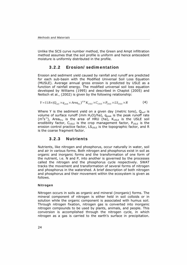
3.2.2 Erosion/sedimentation

Erosion and sediment yield caused by rainfall and runoff are predicted for each sub-basin with the Modified Universal Soil Loss Equation (MUSLE). Average annual gross erosion is predicted by USLE as a function of rainfall energy. The modified universal soil loss equation developed by Williams (1995) and described in Chaplot (2005) and Neitsch et al., (2002) is given by the following relationship:

RLSPCKAreaqQY USLEUSLEUSLEUSLEhrupeaksurf ×××××××= 56.0)(8.11 (4)

Where Y is the sediment yield on a given day (metric tons), Qsurf is volume of surface runoff (mm H2O)/ha), qpeak is the peak runoff rate (m3s-1), Areahru is the area of HRU (ha), KUSLE is the USLE soil erodibility factor, CUSLE is the crop management factor, PUSLE is the erosion control practice factor, LSUSLE is the topographic factor, and R is the coarse fragment factor.

3.2.3 Nutrients

Nutrients, like nitrogen and phosphorus, occur naturally in water, soil and air in various forms. Both nitrogen and phosphorus exist in soil as organic and inorganic forms and the transformation of one form of the nutrient, i.e. N and P, into another is governed by the processes called the nitrogen and the phosphorus cycle respectively. SWAT tracks the movement and transformation of several forms of nitrogen and phosphorus in the watershed. A brief description of both nitrogen and phosphorus and their movement within the ecosystem is given as follows. Nitrogen Nitrogen occurs in soils as organic and mineral (inorganic) forms. The mineral component of nitrogen is either held in soil colloids or in solution while the organic component is associated with humus soil. Through nitrogen fixation, nitrogen gas is converted into inorganic nitrogen compounds to be used by plants, animals, and people. This conversion is accomplished through the nitrogen cycle, in which nitrogen as a gas is carried to the earth’s surface in precipitation.

Chapter 3

25

Nitrogen may also be added to the soil by bacteria fixation, fertilizer and animal manure application. Nitrogen is removed from the soil by denitrification as gaseous loss to the air, plant uptake, soil leaching and surface runoff. The major components of nitrogen cycles are shown in figure 9.

Figure 9: The Nitrogen Cycle (Pidwirny, 2005)

Pertaining to its ability of existing in several chemical valence states, nitrogen is highly reactive and mobile that prediction of its movement between different pools in soil is essential for management with environmental context (Neitsch et al., 2002). SWAT tracks five different pools of nitrogen in the soil: two pools are inorganic compounds (NH4

+ and NO3-), while the other three pools are organic

forms of nitrogen as indicated in figure 10.

Figure 10: SWAT soil nitrogen pools and processes (after Neitsch et al., 2002)

NH4 NO3 Active Stable

Fresh

Mineral N Organic

Volatilization

Inorganic N

Nitrification

Denitrification

Inorganic N

Plant

Mineralization

Humic Residue

Organic N Plant

Residue Mineralization

Decay


26

Nitrate from the mineral N pool (inorganic form) may be transported from soil by surface runoff with water, lateral leaching or percolation to the underlying layer. Howarth (1996) discussed that some of the fertilizer applied to agricultural land leaches directly to groundwater and surface waters depending upon soil characteristics, climate, and crop type and the leaching rate varies from 3 percent to f80 percent of the applied fertilizer. In SWAT, the concentration of nitrate in the mobile water fraction is calculated as:

mobile

lye

mobilely

mobileNO wSAT

wNOConc

∗−−∗

=)1(

exp3

,3

θ (5)

Where concNO3, mobile is the concentration of nitrate in the mobile water for a given layer (kg N/mm H2O), NO3ly is the amount of nitrate in the layer (kg N/ha), wmobile is the amount of mobile water in the layer (mm H2O), εθ is the fraction of porosity from which anions are

excluded, and SATly is the saturated water content of the soil layer (mm H2O). Anions are excluded due to repulsion from particle surfaces or negative adsorption and replaced by cations (Neitsch et al., 2002). The amount of mobile water in the layer is the amount lost by surface runoff, lateral flow or percolation, given by:

lyperclylatsurfmobile wQQw ,, ++= , for top 10mm (6)

lyperclylatmobile wQw ,, += , for lower soil layers (7)

Where wmobile is the amount of mobile water in the layer (mm H2O), Qsurf is the surface runoff generated on a given day (mm H2O), Qlat,ly is the water discharged from the layer by lateral flow (mm H2O), and wperc,ly is the amount of water percolating to the underlying soil layer on a given day (mm H2O). In SWAT the top 10mm soil layer is allowed to interact with the surface runoff and transport nutrients from this layer, which is calculated as:

surfmobileNONOsurf QconcNO ∗∗= ,3 33β (8)

Where NO3surf is the nitrate removed by surface runoff (kg N/ha),

3NOβ is the nitrate percolation coefficient, concNO3,mobile is the

concentration of nitrate in the mobile water for the top 10 mm of soil (mm H2O), and Qsurf is the surface runoff generated on a given day (mm H2O).

Chapter 3

27

Organic form of nitrogen may also be transported by surface runoff attached to soil particles. Organic N is associated with the sediment loading from HRU and any change in sediment loading will be reflected in the loading of this form of nitrogen. SWAT estimates the amount of organic nitrogen loading in surface runoff using a loading function developed by McElroy et al (1976) and modified by Williams and Hann (1978), both cited in Neitsch et al. (2002):

sedNhru

orgNsurf areasedconcorgN :001.0 ∈∗∗∗= (9)

Where orgNsurf is the amount of organic nitrogen transported to the main channel in surface runoff (kg N/ha), concorgN is the concentration of organic nitrogen in the top 10mm (g N/metric ton soil), sed is the sediment yield on a given day (metric tons), areahru is the HRU area (ha), and sedN:ε is the nitrogen enrichment ratio. A larger proportion

of clay sized particles in a sediment load to the main channel leads to the occurrence of a greater proportion or concentration of organic N resulting in the enrichment of organic N. The enrichment ratio is defined as the ratio of concentration of organic nitrogen transported with the sediment to the concentration in the soil surface layer (Neitsch et al., 2002). The concentration of organic nitrogen in the soil surface layer and the nitrogen enrichment ratio are, respectively, calculated in SWAT as:

surfb

surfactsurfstasurffrshorgN depth

orgNorgNorgNconc

.)(

.100 ,,,

ρ++

= (10)

2468.0

, )(78.0 −∗=∈ surqsedNsed conc (11)

Where orgNfrsh,surf is nitrogen in the fresh organic pool in the top 10mm (kg N/ha), orgNsta,surf is nitrogen in the stable organic pool (kg N/ha), orgNact,surf is nitrogen in the active organic pool in the top 10 mm (kg N/ha), bρ is the bulk density of the first soil layer (Mg/m3),

depthsurf is the depth of the soil surface layer (10 mm), and concsed,surq is the concentration of the sediment in surface runoff (Mg sed/m3 H2O). The concentration of sediment in surface runoff is calculated as:


28

surfhrusurqsed Qarea

sedConc∗∗

=10, (12)

Where sed is the sediment yield on a given day (metric ton), areahru is the HRU area (ha), and Qsurf is the amount of surface runoff on a given day (mm H2O). Phosphorus Phosphorus is another key nutrient in soils that occurs in organic form associated with humus, insoluble mineral form and plant available phosphorus in solution. Phosphorus may be added to the soil through the application of fertilizer, manure or residue while removal from the soil occurs by plant uptake and erosion. Phosphorus movement in landscapes is closely associated with soil erosion because P is attached to solid soil materials. Phosphorus reacts readily with positively charged iron (Fe), aluminum (Al), and calcium (Ca) ions to form relatively insoluble substances that precipitate out of solution facilitating the build up of phosphorus near the soil surface that is readily available for transport in runoff (Neitsch et al., 2002). SWAT monitors six pools of phosphorus of which three are organic forms and the remaining three are inorganic forms as shown in figure 11.

Figure 11: SWAT soil phosphorus pools and processes (after Neitsch et al., 2002)

Phosphorus movement in the soil is primarily by diffusion. Surface runoff only partially interacts with the solution P stored in the top 10 mm of soil due to its low mobility. The amount of solution P transported in surface runoff as calculated by SWAT is:

Stable Active Solutio Active Stable Fres

Inorganic P

Plant

Mineral

Mineralization

Residue

Decay

Organic P Plant id

Humic Residu

Organic

Chapter 3

29

surfdsurfb

surfsurfsolutionsurf kdepth

QPP

,

,

***

ρ= , (13)

Where Psurf is the amount of soluble phosphorus lost in surface runoff (kg P/ha), Psolution,surf is the amount of phosphorus in solution in the top 10mm (kg P/ha), Qsurf is the amount of surface runoff on a given day (mm H2O), bρ is the bulk density of the top 10 mm (Mg/m3),

depthsurf is the depth of the surface layer (10 mm), and kd,surf is the phosphorus soil partitioning coefficient (m3/Mg). The amount of organic and mineral P that is transported attached to the sediment particles is calculated by SWAT using the loading function developed by McElroy et al (1976) and modified by Williams and Hann (1978), cited in Neitsch et al. (2002):

sedphru

sedPsurf areasedconcsedP :***001.0 ∈= , (14)

Where sedPsurf is the amount of phosphorus transported with sediment to the main channel in surface runoff (kg P/ha), concsedP is the concentration of phosphorus attached to sediment in the top 10 mm (g P/metric ton soil) calculated using equation 12, sed is the sediment yield on a given day (metric tons), areahru is the HRU area (ha), and sedp:ε is the phosphorus enrichment ratio calculated using

the same equation (11) for N above. The concentration of phosphorus attached to sediment in the soil surface layer, concsedP, is computed as:

surfb

surffrshsurfhumsurfstasurfactsedP depth

orgPorgPPPconc

*)min(min

*100 ,,,,

ρ+++

= , (15)

Where minPact,surf is the amount of phosphorus in the active mineral pool in the top 10 mm (kg P/ha), minPsta,surf is the amount of phosphorus in the stable mineral pool in the top 10 mm (kg P/ha), orgPhum,surf is the amount of phosphorus in the humic organic pool in the top 10 mm (kg P/ha), orgPfrsh,surf is the amount of phosphorus in the fresh organic pool in the top 10 mm (kg P/ha), bρ is the bulk

density of the first soil layer (Mg/m3), and depthsurf is the depth of the soil surface layer (10 mm).


30

3.3 Model Inputs

SWAT requires specific information about watershed characteristics such as topography, land use/cover, soil types, weather, and management practices. The model uses a two-level discretization scheme; first basin and sub-basin delineation is performed based on topographic information, followed by further discretization into HRUs using land use and soil type considerations in order to represent heterogeneous watershed properties. Climate inputs are required since they control water balance that drives all the processes simulated in the watershed. Management practice of a watershed is needed because it greatly influences the nutrient emission to surface and subsurface waters.

3.3.1 Watershed Delineation

The subdivision of a watershed into discrete sub-watershed areas enables the modelling process to represent, as much as possible, the heterogeneity of the watershed. SWAT works on a sub-basin basis and the interface delineates the watershed into such sub-basins or sub-watersheds based on topographic information. The delineation of Rönne watershed was performed based on topographic information of the watershed area obtained from the Swedish Land Survey Department in the form of digital elevation model (DEM) with X-Y resolution of 50 metres using the procedure described in ArcView interface for SWAT2000 user’s guide (DiLuzio et al., 2002). The total watershed area of Rönne basin is about 190000 ha (VASTRA, 2005) while that of total delineated area by the algorithm was 180500 ha. The discrepancy between the actual and the delineated area could be due to the fact that some modifications were made to the original DEM data to allow complete delineation of the entire watershed area which otherwise disallows the delineation of the most downstream or the main outlet area. The reason was that some cells had zero values near the outlet which persisted even after the pre-processing of the DEM to remove sinks by the interface. The application of one time 3x3 low pass filter in ArcGIS to the DEM was able to solve the problem by averaging the cells having 0 values with surrounding pixels. Since the size of a sub-basin is believed to affect the assumption of homogeneity or spatial variability of conditions (Jha et al., 2004), definition of the watershed, sub-basin boundaries and streams was made by selecting a threshold area or the minimum draining area to define streams. Configuration of larger number of sub-basins causes

Chapter 3

31

an increased amount of input data preparation and subsequent analysis though detailed spatial variations with in the watershed could be simulated. On the other hand, too small number of sub-watersheds could affect the simulation result by ignoring spatial variability that lumps watershed conditions together. Therefore, a threshold level and hence the number of sub-basins for a given watershed area needs to be selected carefully, and (Jha et al., 2004) suggested a maximum of 35 and 11 sub-basins for predicting nitrate and mineral P losses respectively for watersheds approximately comparable in size to the present study area. For the present sub-watershed configuration, a threshold area of 4500 ha was used to generate a reasonable number of sub-basins with additional sub-basins delineated to obtain output at 8 water quality monitoring stations for nutrient, especially nitrate, loading simulation. Although the interface could automatically generate sub-basin outlets, manual edition was made in order to include additional outlets at key locations of water quality monitoring sites and remove some of the automatically generated ones so that the desired size of sub-basins would be delineated. Subsequently, selection of the main watershed outlet was made to delineate the main watershed area and 21 sub-basins. Before the task of delineating the main watershed area and sub-basins has been completed, locations of water quality monitoring sites were added into the configuration for simulation and comparison at a later stage of the modelling process. The digital elevation model and the subsequently delineated watershed, sub-basins, streams, selected sub-basin outlet locations and SWAT weather generator locations are shown in figure 12. The statistical summary of topographic data (elevation report) for the delineated watershed and sub-basins is given in appendix 1.


32

Figure 12: DEM (left) and the delineated watershed/sub-basins (right).

3.3.2 Land Use and Soil Characterization

Land cover and soil, among others, greatly influence the hydrological properties of a watershed that they are two of the five main input datasets required by SWAT to help describe a sub-basin or HRU. Once watershed topographic parameters have been computed for each sub-basin, the interface uses land cover and soils data to generate multiple hydrologic response units (HRUs) within each sub-basin by GIS overlay process to assign soil parameters and SCS curve numbers. HRUs are lumped land areas within the sub-watershed that are comprised of distinctive land cover, soil, and management combinations (Neitsch et al., 2002). Such subdivision of sub-basins into HRUs enables the SWAT model to reflect the spatial variations of the hydrologic conditions for different land cover and soil distributions within the sub-basins Land Cover Data Land cover information for the study area was downloaded from The European Topic Centre on Terrestrial Environment (CORINE land cover database) owned by European Environment Agency (EEA,

Chapter 3

33

2000). CORINE is a European Commission programme established with the aim of compiling and coordinating information on the state of the environment and ensuring that the information are consistent and data are compatible within the Member States of the Community as well as at international level. The land cover project is part of the CORINE programme intended to provide consistent geographical information on the land cover of the Member States of the European Community, which is believed to be essential for the management of the environment and natural resources. This data was chosen to be used as model input because: • It is freely available for the Member States of the Community that

downloading from Internet was easily possible through the GIS Centre of Lund University.

• It provides the user with an option in his/her best interest of spatial details to be used by the model.

• It is compatible with most GIS softwares so that data extraction and preparation for the SWAT model input is easier.

• It has been compiled with the aim of providing reliable land cover information to help decision-making process for environmental and natural resources management.

All features in CORINE land cover map were extracted from an interpretation of satellite images, namely Landsat and Spot images, aided by topographic maps obtained from different countries of the Member States and the map has been compiled with various scales and different level of details (3 levels), the surface area of the smallest unit mapped being 25 hectares, to enable decision-makers to identify, analyse and monitor land use management systems. Level 1 is highly generalised information indicating the major categories of land cover while level 2 with 15 land use classes has been compiled for use on scales of 1:500000 and 1:1000000. The third level, with 44 land use classes, is a larger scale map describing more detailed features that can be used for projects on a scale of 1:100000. The different level of details and nomenclature for CORINE land cover is shown in table 4. A simplified form of the level 2 CORINE land use nomenclature was established for this study. The modification was important because firstly the SWAT input land use data should, more or less, match with that of the SWAT land cover database used by the model, secondly since the data was extracted from a large area covering southern part of Sweden, some of the classes were absent or are not common in the study area, and thirdly minor land use classes would be eliminated at a later stage during definition of the land use/soil distribution or HRUs depending on the selected threshold.


34

Table 4: CORINE land cover nomenclature Level 1 Level 2 Level 3

1.1.1. Continuous urban fabric 1.1. Urban fabric 1.1.2. Discontinuous urban fabric 1.2.1. Industrial or commercial units 1.2.2. Road and rail networks and associated land 1.2.3. Port areas

1.2. Industrial, commercial and transport units

1.2.4. Airports 1.3.1. Mineral extraction sites 1.3.2. Dump sites

1.3. Mine, dump and construction sites

1.3.3. Construction sites 1.4.1. Green urban areas

1. Artificial surfaces

1.4. Artificial non-agricultural vegetated areas

1.4.2. Sport and leisure facilities

2.1.1. Non-irrigated arable land 2.1.2. Permanently irrigated land

2.1. Arable land

2.1.3. Rice fields 2.2.1. Vineyards 2.2.2. Fruit trees and berry plantations

2.2. Permanent crops

2.2.3. Olive groves 2.3. Pastures 2.3.1. Pastures

2.4.1. Annual crops associated with permanent crops 2.4.2. Complex cultivation 2.4.3. Land principally occupied by agriculture, with significant areas of natural vegetation

2. Agricultural areas

2.4. Heterogeneous agricultural areas

2.4.4. Agro-forestry areas 3.1.1. Broad-leaved forest 3.1.2. Coniferous forest

3.1. Forests

3.1.3. Mixed forest 3.2.1. Natural grassland 3.2.2. Moors and heathlands 3.2.3. Sclerophyllous vegetation

3.2. Shrub and/or herbaceous vegetation association

3.2.4. Transitional woodland shrub 3.3.1. Beaches, dunes and sand plains 3.3.2. Bare rock 3.3.3. Sparsely vegetated areas 3.3.4. Burnt areas

3. Forests and semi-natural areas

3.3. Open space with little or no vegetation

3.3.5. Glaciers and perpetual snow 4.1.1. Inland marshes 4.1. Inland wetlands 4.1.2. Peatbogs 4.2.1. Salt marshes 4.2.2. Salines

4. Wetlands

4.2 Coastal wetlands

4.2.3. Intertidal flats 5.1.1. Water courses 5.1. Inland waters 5.1.2. Water bodies 5.2.1. Coastal lagoons 5.2.2. Estuaries

5. Water bodies

5.2. Marine waters

5.2.3. Sea and ocean Source: (EEA, 2000)

Chapter 3

35

Therefore, ArcView GIS was used to reclassify and prepare the data input as required, considering 7 main classes: urban, agriculture, pasture, shrub/range, forest, wetland and water. All the artificial surfaces with built-up areas were summarised as and designated by urban residential-medium to low density; arable land and permanent crops as agricultural land-generic; pastures as pastures; forests as forest-mixed; shrub and/or herbaceous vegetation association and open space with little or no vegetation as range-brush; inland wetlands as wetlands-mixed and inland waters as water. Some of the classes not mentioned here from the level 2 of the CORINE land cover nomenclature are missing in the study area. In the subsequent discussion, reference will be made to the generalised land use map of the study area with 7 classes, characterised mainly by forest (46.7%) and arable land (26.6%), both comprising about 73% of the total watershed area. The rest of land use types occupy a very less proportion: pasture (8.5%), brush and rangeland (8.6%), urban areas (4.5%), water bodies (3.5%) and wetlands (only 1.6%), as quantified by SWAT in ArcView interface. Figure 13 shows the reclassified land use map while the proportion of each land use and their description is given in table 5.

Table 5: Proportion and description of the newly classified land use types from CORINE No. Area (%) Swat Land Class Description 1 4.53 URML Residential-Med/Low Density 2 26.57 AGRL Agricultural Land-Generic 3 8.49 PAST Pasture 4 46.74 FRST Forest-Mixed 5 8.57 RNGB Range-Brush 6 1.62 WETL Wetlands-Mixed 7 3.48 WATR Water

Total 100.00 After preparing the land use data to be used in the model, a semi-supervised satellite image classification of the study area, based on few GPS points (only about 26), was performed to have a quick overview and compare with CORINE land cover map. This was to show if semi-supervised maps, with less cost and time, could be used as model input in the absence of carefully prepared maps. The size of ground truth sample was limited to only few points because of time constraint to carryout intensive fieldwork. Landsat 7 ETM+ image from the year 1999 was downloaded from the University of Maryland database, which is freely available for the geo-information community (University of Maryland, 2005). Since it has already been geo-referenced and rectified, pre-processing was not required that only


36

the area of interest (AOI) was clipped and the coordinate system was re-projected to fit that of the Swedish National Grid. ERDAS software was used for the classification procedure. The resulting classified land use map was somewhat similar to that of the CORINE data whereby most classes were noticeably identified. The satellite image and the resulting classified land use map are attached in appendix 2.

Figure 13: Generalised land use map used as model input

Soil Data Soil data was obtained from the Geological Survey of Sweden (Sveriges Geologiska Undersökning-SGU) through the GIS Centre of the Lund University. The data was in digital format having different level of soil classes that enables modification according to the interest

Chapter 3

37

of users and the SWAT input data format. The more generalised soil class comprises 14 soil types including water covered areas. The soils are geologically young and belong to the Quaternary period, formed during the ice age (glacial soils) and subsequent processes (post glacial soils). The glacial soils contain tills/moraines and glacial sediments. Tills are the most common soil types and are mainly clayey (Gustafsson, 1992), but some times also occur as sandy or sandy-silty in some places (Norling and Wikman, 1990) that led to classify them as clay in this study. The glacial sediments consist of coarse grained sediments- sand, gravel, and cobbles, and of fine grained sediments-clay and silt, which were classified as sand for the purpose of this study. The postglacial soils can be divided into re-worked and redeposited types and organic soils. After the glaciation period, there was a strong increase in the production of organic material mixed into the fine grained material to form organic fine grained soils, e.g. organic clay and peat bogs sporadically distributed within the watershed area. A typical soil profile, in the study area, from top to bottom is characterised by organic soil; postglacial and glacial clay; stones, gravel and sand; till and finally bed rock. The most common soil types of the study area, based on the 14 classes of SGU, are indicated in table 6.

Table 6: Common soil types of the Rönne watershed No. Soil type Description Generalised as 1 Organic Soil Organic clay, peat bogs, swamps Organic Soil 2 Clay Glacial and postglacial clay Clay 3 Silt Glacial and postglacial silt Silt 4 Sand Glacial sand Sand 5 Gravel Glacial gravel Sand 6 Stone block Postglacial stone blocks Rock 7 Fluvioglacial

sediment Mostly glacial sand with gravels Sand

8 Moraine clay Moraine; clay >15% Clay 9 Moraine Moraine; range from fine grained

clays to coarse grained gravel tills. Clay

10 Thin earth layer Missing in the study area -

11 Rock outcrop bedrock Rock 12 Landfills Land fill, natural or artificial Sand 13 Others Unknown under water Water 12 Water Water bodies Water A simplified classification of soils is important in order to avoid further complications and extensive data input demand by the model during soil parameterization. Furthermore, some of the soil types, listed in table 7, are insignificant in terms of proportion in the study area while some of them are closely similar to others in terms of soil physical


38

properties, such as texture, which is the most important soil parameter in SWAT. Therefore, the original SGU soil data was reclassified into 6 soil types, mainly based on texture. Water was considered as one class in this study because of its unique effect on nutrient movement as the different types of soils do. Figure 14 shows the reclassified soil types while the proportion of each soil type and their description is given in table 7.

Figure 14: A generalised map of soil types used as model input

According to the newly classified soil types, most of the watershed area is occupied by clayey soils of mainly moraine type (60%) while sandy soils occupy about 20% of the watershed. Organic soils cover about 12%, sporadically distributed over the whole area and a less proportion of the area is made up of the rest minor classes.

Chapter 3

39

Table 7: Proportion and description of the newly classified soil types used as model input No. Area (%) Swat Soil Class Description 1 11.96 Organic soil Peat bogs, swamps 2 59.93 Clay Mainly moraine clay 3 2.65 Silt Glacial and fluvial origin 4 20.60 Sand Glacial sand, moraine,

sediments and gravels 5 1.11 Rock Rock outcrops and boulders 7 3.75 Water Water bodies and soils under

water Total 100.00 Various physical properties such as bulk density, available water capacity, saturated hydraulic conductivity, k-factor and organic carbon content are required by SWAT in order to carry out the modelling process. The characterisation of the different soil parameters was made by making use of a graphic computer programme known as soil water characteristics (Saxton, 2003). The programme estimates moist bulk density, available water capacity and saturated hydraulic conductivity using the soil texture and organic matter. The soil types were used to derive soil textures while the soil organic matter content for Sweden, given in literature, was used. The median value of organic matter content for most Swedish arable land, including organic soils, is 4.1%; and for soils with less organic matter, the median value is 3.9% (Eriksson et al., 1997). USLE soil erodibility factor or k-factor was collected from various sources for different soil textures. Table 8 shows the different soil parameters used for the current study. Finally, since there were no available data on different soil layers, only a single soil layer was assumed over the entire watershed for the modelling purpose. In fact, there is no well developed soil layer in the study area since the soils are of much younger age associated to the glacial and post-glacial geological activities.

Table 8: Estimated soil parameters for main soil textures Soil Type Soil

group BD

g/cm3 AWC

mm/mm Ks

mm/hr CBN %

Clay %

Silt %

Sand %

k-factor

Organic Soil C 1.1 0.15 33.3 4.1 40 30 30 0.15 Clay C 1.10 0.14 26.50 4.10 50 25 25 0.15 Silt B 1.20 0.24 298.50 3.90 15 15 70 0.42 Sand A 1.33 0.15 145.30 3.90 10 10 80 0.10 Rock D 2.30 0.04 0 0.10 7 3 90 0.01 Water D 1.10 0.15 13 - - - - 0.05 Note: some parameters were changed during calibration


40

GIS overlay of the land cover and soil information

Once the land cover and soil datasets have been prepared in a format that can be used by the SWAT2000 model, overlay of the two GIS layers was made by the interface to generate detailed land use and soil distribution for the entire watershed area and the 21 sub-basins defined during the watershed delineation stage. This was followed by definition of multiple HRUs within sub-basins. Since the user is allowed to decide whether or not to use HRUs in the modelling application, in this study it was preferred to proceed with the definition of HRUs so that spatial differences of hydrological processes within sub-basins would be reflected. If multiple HRUs are ignored, the interface will use the dominant land use and soil characteristics for the entire watershed which ignores the spatial variability by lumping together the sub-basin processes. A threshold level can also be determined by the user to model multiple HRUs by eliminating minor land uses in each sub-basin. Subsequently, land uses that cover a percentage of the sub-basin area less than the threshold level are eliminated and the area of the land use is reapportioned so that 100 percent of the land area in the sub-basin is included in the simulation. It has been suggested (DiLuzio et al., 2002) that a 20 percent land use threshold and a 10 percent soil threshold are adequate for most modelling applications. However, a 10 percent land use and a 10 percent soil threshold were used in this simulation so that more detailed discretization of sub-basins would be possible to represent more heterogeneous watershed attributes, which resulted in 127 unique land use/soil combinations or HRUs.

3.3.3 Climate Data

Weather data is another key set of input data required by SWAT2000 model. The daily climate inputs include precipitation, maximum and minimum temperature, solar radiation, wind speed and relative humidity. They can be supplied to the model in two general ways: (1) from daily observations of historical data recorded at specific stations near or within the watershed as a user-specified file or (2) monthly statistical data on local weather conditions after which SWAT weather generator simulates the time series data. A combined approach was used in this study where daily precipitation data for the period 1981-2000, obtained from the Swedish Meteorological and Hydrological Institute, was supplied to the model while the rest were left to be generated internally within SWAT for the 40 year period after providing monthly weather statistical data at three locations within the watershed. Most of the statistical datasets were obtained from internet sources, such as WORLDCLIM (Hijmans et al., 2004) for

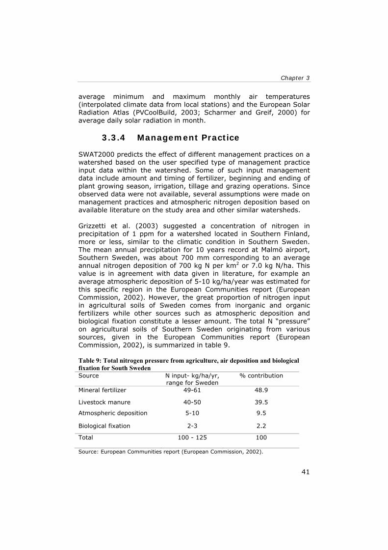
Chapter 3

41

average minimum and maximum monthly air temperatures (interpolated climate data from local stations) and the European Solar Radiation Atlas (PVCoolBuild, 2003; Scharmer and Greif, 2000) for average daily solar radiation in month.

3.3.4 Management Practice

SWAT2000 predicts the effect of different management practices on a watershed based on the user specified type of management practice input data within the watershed. Some of such input management data include amount and timing of fertilizer, beginning and ending of plant growing season, irrigation, tillage and grazing operations. Since observed data were not available, several assumptions were made on management practices and atmospheric nitrogen deposition based on available literature on the study area and other similar watersheds. Grizzetti et al. (2003) suggested a concentration of nitrogen in precipitation of 1 ppm for a watershed located in Southern Finland, more or less, similar to the climatic condition in Southern Sweden. The mean annual precipitation for 10 years record at Malmö airport, Southern Sweden, was about 700 mm corresponding to an average annual nitrogen deposition of 700 kg N per km2 or 7.0 kg N/ha. This value is in agreement with data given in literature, for example an average atmospheric deposition of 5-10 kg/ha/year was estimated for this specific region in the European Communities report (European Commission, 2002). However, the great proportion of nitrogen input in agricultural soils of Sweden comes from inorganic and organic fertilizers while other sources such as atmospheric deposition and biological fixation constitute a lesser amount. The total N “pressure” on agricultural soils of Southern Sweden originating from various sources, given in the European Communities report (European Commission, 2002), is summarized in table 9.

Table 9: Total nitrogen pressure from agriculture, air deposition and biological fixation for South Sweden Source N input- kg/ha/yr,

range for Sweden % contribution

Mineral fertilizer 49-61 48.9

Livestock manure 40-50 39.5

Atmospheric deposition 5-10 9.5

Biological fixation 2-3 2.2

Total 100 - 125 100

Source: European Communities report (European Commission, 2002).


42

Since detailed information was not available on arable crop land distribution, a generic agricultural land (AGRL- equivalent to 4 character SWAT2000 land cover code) and pasture grass (PAST) were chosen to represent agricultural lands. The crops were assumed to grow in the middle of May after fertilizer operation. A fertilizer application was considered for generic agricultural land use and pasture grasses. The maximum fertilizer input rate (125 kg N/ha/yr) was used as model input because the study area is a relatively densely populated and intensely cultivated area due to the presence of favourable fertile soil for agriculture compared to other parts of Sweden. The timing of tillage operation, crop growth, fertilizer application, and harvesting is given in table 10, based on assumption in Southern Finland as mentioned by Grizzetti et al. (2003) and Southern Sweden (European Commission, 2002; VASTRA, 2005).

Table 10: Schedule of tillage, planting, fertilizer application and harvesting for model runs Year Date Operation

May 3 Chisel Plow May 14 Fertilization (125 kg/ha) May 17 Plant Spring Barley August 26 Harvest Barley

1

September 01 Tillage operation

3.4 Model Calibration and Validation

Once the main SWAT input data are ready to successfully run the model, a number of output files are generated after simulation. The main SWAT output files generated during simulation are indicated in appendix 3. Model calibration and validation was performed based on these output files. Model calibration is a procedure to adjust or fine-tune model parameters so as to represent observed conditions in as much as possible, while validation is testing of the calibrated model results with independent data set without any further adjustment (Neitsch et al., 2002) at different spatial and temporal scales. In water quality modelling, a three step calibration procedure has been suggested by Neitsch et al. (2002), first starting with water balance and stream flow followed by sediment and nutrient consecutively. However, the availability of observed data set determines whether to perform the calibration on all or part of the procedures suggested. After the initial configuration of SWAT, model calibration and validation were performed on selected locations within the watershed. Stream flow was calibrated first, then nutrient concentration was considered, while sediment was excluded since measured time series

Chapter 3

43

data was not available for calibration purposes. Stream flow was calibrated on annual and monthly average time steps at two locations while NO3 was calibrated at one location on monthly basis. The calibration and validation locations are indicated in figure 15.

Figure 15: Model calibration and validation sites (the numbers represent designated sub-basins)

The model was first calibrated for flow at the outlet of sub-basin 15 (here after referred as Ringsjön) representing five upstream sub-basins, then extended to the outlet of sub-basin 19 (here after referred as Klippan basin) located further downstream of Ringsjön. The already calibrated parameters, on upstream site, were kept unchanged during calibration of the downstream site. The two calibration sites were selected primarily due to the availability of measured daily stream flow data for a period of 20 years (Jan 1981–


44

Dec 2000) which was acquired from the VASTRA project of the Swedish Meteorological and Hydrological Institute. Regarding temporal scale, long-term average annual stream flow was calibrated first and after ensuring the satisfactory performance of the model for the yearly time step, monthly stream flow was calibrated for each location again without changing the values already adjusted during yearly time step. The period from 1981-1990 was used for calibration while validation was performed during the period 1991-2000. Key hydrologic parameters such as SCS runoff curve number for moisture condition II, available water capacity of the soil layer, ground water revaporation coefficient and the threshold depth of the shallow aquifer before evaporation can occur were considered for flow calibration. The parameters were chosen based on previous researched works on SWAT calibration (Jha et al., 2004; Santhi et al., 2005) and suggestions given by Neitsch et al. (2002). The values or ranges of selected sensitive parameters before and after calibration are given in table 11. These parameters were believed to govern the partitioning of precipitation between surface and ground water flows (Tetra Tech Inc., 2004) and hence are sensitive components.

Table 11: Initial and final values of SWAT calibration parameters for stream flow Variable name

Description Recommended Range

Initial value

Calibrated value

CN2 SCS runoff curve number for antecedent moisture condition II

±8 - -8

SOL_AWC Soil available water capacity

±0.05 - 0.05

ESCO Soil evaporation compensation factor

0-1 0 0.1

GW_REVAP Ground water revaporation coefficient

0.02-0.2 0.02 0.1

CH_K2 Effective hydraulic conductivity in main channel alluvium

-0.01-150 0 50

ALPHA_BF Baseflow alpha factor 0-1 0.048 1 SMFMX Maximum melt rate

for snow during the year

0-10 4.5 10

SMFMN Minimum melt rate for snow during the year

0-10 4.5 10

SLOPE Average slope steepness

0-0.6 0.025 0.2

SLSUBBSN Average slope length 10-150 91.5 50

Chapter 3

45

After confirming that the stream flow calibration results were reasonably convincing and adequate, attempt was made to calibrate nutrient (NO3-N) concentration in stream water at the outlet of Klippan sub-basin. The calibration process involved comparing water quality time series simulation output to available water quality (NO3 concentration) observation data, obtained from VASTRA. The available measured water quality data was not a continuous daily record of monitoring data for nutrients. Only about 12 sample data per year (grab samples) were available from the monitoring station for the period Jan 1997-Dec 2000. Additional data on point sources pollution were not also available, whereas it was learned that two such sources from municipal waste water treatment plants exist within the sub-basin. Since point source emissions are believed to greatly influence the concentration of nutrients in streams, comparison of observed and simulated water quality without considering point sources would not be as such meaningful. However, since point sources are expected to be controlled emissions, i.e. constant daily discharges, significant temporal variation is not expected on the model output as a result of the missing data. Nevertheless, in order to best reproduce the observed data by simulation, fine tuning of pollutant loading and in-stream water quality parameters within recommended range were performed. The SWAT parameters related to nutrient loading such as nitrogen percolation factors (NPERCO), initial organic nutrient concentration in surface soil layer (SOL_ORGN), initial mineral nutrient concentration in the soil layer (SOL_NO3), biological mixing efficiency (BIOMIX) and fertilizer application rates were adjusted. Although the model was found to be very sensitive to NPERCO and slightly to fertilizer application rates, the remaining parameters were not responsive and much improvement could not be achieved in reproducing the observed scenarios. Validation was not performed for nitrate because of the unavailability of sufficient data as well as due to the poor results obtained on calibration. Finally, calibration and validation results were evaluated by comparing time series model outputs to measured data. Graphical comparison and statistical analysis methods were used to test for goodness-of-fit. It has been suggested that graphical comparison is enormously useful for judging the results of model calibration as it provides a good visual control over time-variable plots of measured against simulated flow and the model’s capability to reproduce storm hydrographs, base flow recession, time lags, and other related factors, which are often overlooked by statistical comparisons (Tetra Tech Inc., 2004). Several statistical methods including the Nash-


46

Sutcliffe prediction efficiency (ENS), coefficient of determination (r2), mean error, root mean square error, root mean square, etc, are available for evaluating the model predictions versus the observed values. The first two statistical approaches, ENS and r2, were used here since they are the most commonly used methods in several other similar studies. The Nash-Sutcliffe prediction efficiency (Nash and Sutcliffe, 1970) indicates how well the plot of observed against simulated value fits the 1:1 line, which is computed as:

∑∑

=

=

−

−−= n

i i

n

i iiNS

QQ

QQE

12

12

)(

)'(1 , (16)

Where Q represents the mean measured values, Qi and Q’i are the measured and simulated values respectively and n is the number of values computed. A value for ENS equal to 0 or less indicates a poor performance of the model while a value of 1 indicates a perfect fit between the measured and model predicted values. The second statistical goodness-of-fit used was the coefficient of correlation (r2), which explains how much the measured values are explained by the simulated values indicating the strength of correlation between the two variables. If the value for r2 is zero or close to zero, the model’s prediction capability is poor and unacceptable. If the values are close or equal to one, the model prediction is considered perfect.

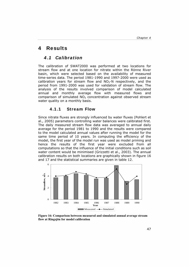
Chapter 4

47

4 Results

4.1 Calibration

The calibration of SWAT2000 was performed at two locations for stream flow and at one location for nitrate within the Rönne River basin, which were selected based on the availability of measured time-series data. The period 1981-1990 and 1997-2000 were used as calibration years for stream flow and NO3-N respectively, and the period from 1991-2000 was used for validation of stream flow. The analysis of the results involved comparison of model calculated annual and monthly average flow with measured flows and comparison of simulated NO3 concentration against observed stream water quality on a monthly basis.

4.1.1 Stream Flow

Since nitrate fluxes are strongly influenced by water fluxes (Pohlert et al., 2005) parameters controlling water balances were calibrated first. The daily measured stream flow data was averaged to annual daily average for the period 1981 to 1990 and the results were compared to the model calculated annual values after running the model for the same time period of 10 years. In computing the efficiency of the model, the first year of the model run was used as model priming and hence the results of the first year were excluded from all computations so that the influence of the initial conditions such as soil water content would be minimised (Grizzetti et al., 2003). The annual calibration results on both locations are graphically shown in figure 16 and 17 and the statistical summaries are given in table 12.

0

2

4

6

1982 1983 1984 1985 1986 1987 1988 1989 1990Year

Stre

amflo

w,

m3 /s

Measured Simulated

Figure 16: Comparison between measured and simulated annual average stream flow at Ringsjön for model calibration

Results

48

0

1

2

3

4

5

1982 1983 1984 1985 1986 1987 1988 1989 1990Year

Stre

amflo

w, m

3 /s

Measured Simulated

Figure 17: Comparison between measured and simulated annual average stream flow at Klippan for model calibration

Figures 16 and 17 show the time-series comparison of model simulated and observed annual stream flows for the Ringsjön and Klippan locations respectively over the 10 year (1981-1990) calibration period. Generally, the model performed satisfactorily by closely tracking the observed annual flows. There was a good match between the observed and simulated flow values both in magnitude and temporal variations at both locations although some peak flows tended to be under predicted and some of the low flows were over predicted.

Table 12: Summary of calibration results for annual stream flows (m3/s) at Ringsjön and Klippan

Performance

Loca

tion

Yea

r

1982

1983

1984

1985

1986

1987

1988

1989

1990

ENS R2

Meas. 3.70 3.97 4.41 4.13 3.51 3.61 5.80 3.10 3.37

Rin

gsj

ön

Sim. 3.98 4.10 4.72 4.34 3.70 3.77 5.20 2.60 3.96

0.75

0.77

Meas. 2.98 3.42 3.16 3.87 2.82 3.01 4.11 2.33 2.86

Klip

pan

Sim. 2.91 3.28 3.38 3.49 3.19 2.85 4.12 2.39 3.23

0.78

0.79

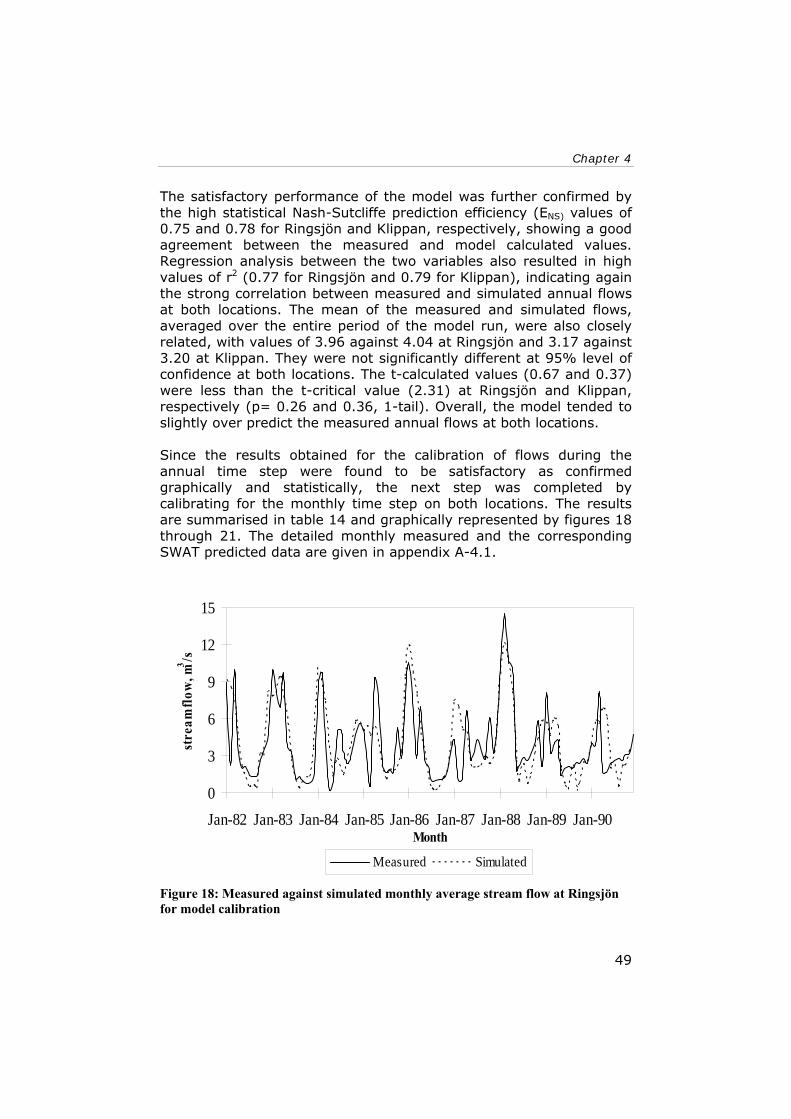
Chapter 4

49

The satisfactory performance of the model was further confirmed by the high statistical Nash-Sutcliffe prediction efficiency (ENS) values of 0.75 and 0.78 for Ringsjön and Klippan, respectively, showing a good agreement between the measured and model calculated values. Regression analysis between the two variables also resulted in high values of r2 (0.77 for Ringsjön and 0.79 for Klippan), indicating again the strong correlation between measured and simulated annual flows at both locations. The mean of the measured and simulated flows, averaged over the entire period of the model run, were also closely related, with values of 3.96 against 4.04 at Ringsjön and 3.17 against 3.20 at Klippan. They were not significantly different at 95% level of confidence at both locations. The t-calculated values (0.67 and 0.37) were less than the t-critical value (2.31) at Ringsjön and Klippan, respectively (p= 0.26 and 0.36, 1-tail). Overall, the model tended to slightly over predict the measured annual flows at both locations. Since the results obtained for the calibration of flows during the annual time step were found to be satisfactory as confirmed graphically and statistically, the next step was completed by calibrating for the monthly time step on both locations. The results are summarised in table 14 and graphically represented by figures 18 through 21. The detailed monthly measured and the corresponding SWAT predicted data are given in appendix A-4.1.

0

3

6

9

12

15

Jan-82 Jan-83 Jan-84 Jan-85 Jan-86 Jan-87 Jan-88 Jan-89 Jan-90Month

stre

amflo

w, m

3 /s

Measured Simulated

Figure 18: Measured against simulated monthly average stream flow at Ringsjön for model calibration

Results

50

0

2

4

6

8

10

12

14


Stre

amflo

w (m

3 /s)

Measured Simulated

Figure 19: Measured against simulated monthly average stream flow at Klippan for model calibration

The predicted result was able to satisfactorily reproduce and closely follow the corresponding observed monthly flows. The peak flows and temporal variations were well tracked by the model, with some over- and under-predictions, at both locations, the comparisons of which are shown in figure 18 and 19. The monthly predicted values were also regressed and plotted against the measured flows and figure 20 and 21 provide their distribution along the 1:1 line for the two calibration sites. The results showed that the measured and calculated flows were uniformly distributed along the 1:1 line without any significant outlier, indicating a good level of agreement between the observed and simulated values.

0

3

6

9

12

15

0 3 6 9 12 15Measured flow (m3/s)

Sim

ulat

ed fl

ow (m

3 /s)

regression line 1:1 line

Figure 20: Regression and 1:1 line fit plot of observed versus simulated monthly stream flow at Ringsjön, Jan 1981 to Dec 1990

Chapter 4

51

0

2

4

6

8

10

12

14

0 2 4 6 8 10 12 14Measured flow (m3/s)

Sim

ulat

ed fl

ow (m

3 /s)


Figure 21: Regression and 1:1 line fit plot of observed versus simulated monthly stream flow at Klippan, Jan 1981 to Dec 1990

Further statistical test for goodness-of-fit, provided in table 13, showed that the Nash-Sutcliffe values of 0.35 for Ringsjön and 0.53 for Klippan were lower as compared to the annual performance of the model, but still considered satisfactory and acceptable. The results of regression analysis, with r2 values of 0.52 and 0.63 for Ringsjön and Klippan respectively, also showed a good correlation between predicted and measured values for the indicated time step. The mean of the measured and simulated flows, averaged over the entire simulation period, were also closely related with values of 3.96 against 4.05 at Ringsjön and 3.28 against 3.21 at Klippan. They were not significantly different at 95% level of confidence (α =0.05) at both locations since the t-calculated values of 0.40 and 0.44 were less than the t-critical values of 1.66 at both Ringsjön and Klippan, respectively (p= 0.34 and 0.33, 1-tail test). Overall, the model tended to slightly under predict high flows.

Table 13: Summary of calibration results for monthly stream flows at Ringsjön and Klippan

Mean 1-tail t-test, α =0.05 Performance Location No. of observations Meas. Sim. t-calc t-

crit p-value

ENS R2

Ringsjön 108 3.96 4.05 0.40 1.66 0.34 0.35* 0.52*

Klippan

108 3.28 3.21 0.44 1.66 0.33 0.53 0.63

*The initial calibration results (ENS=0.50 and r2=0.57) were affected during calibration on downstream sub-basin at Klippan.

Results

52

4.1.2 Nutrient (NO3-N)

Nitrate was considered for nutrient calibration based on the availability of observed stream water quality data. Since the measured nitrate data was concentration in g/l, the SWAT simulated NO3 load (kg N) was converted to concentration by dividing with the simulated flow out of the reach at Klippan using a concentration–load relationship as:

QFC = (17)

Where, C is nitrate concentration in stream water (g/l), F is nitrate transported with water out of reach during the simulation time step (e.g. kg N/month) and Q is stream flow out of reach during the time step (e.g. m3/month). The predicted results were compared with the observed data on a monthly basis for the period of Jan 1997-Dec 2000. The result showed a poor agreement between the observed and measured values by consistently under predicting the observed data, as expected, regardless of efforts made to verify all the key processes related to nutrients. Nutrient parameter adjusted was only the nitrogen percolation factor (NPERCO) which was found to be the only sensitive variable while others such as SOL-NO3, BIOMIX, RSDCO and fertilizer application rates remained unresponsive or very slightly if any at all. However, the simulated concentration tends to reflect the seasonality of the measured data. Figure 22 shows comparison of observed and simulated monthly NO3 concentration at the outlet of Klippan sub-basin. The detailed monthly measured and the corresponding SWAT predicted data are given in appendix A-4.3.

0

1

2

3

Jan-98 Jul-98 Jan-99 Jul-99 Jan-00 Jul-00

Month

NO

3 (m

g/l)

0

0.5

1

1.5

2

NO

3 (m

g/l)

measured simulated

Figure 22: Observed against simulated NO3-N concentration in stream water at Klippan

Chapter 4

53

The poor agreement between the observed and simulated values was an expected result due to uncertainties associated to the data used for model input as already mentioned in section 3.4. First, the measured data were not continuous daily records of monitoring data (only grab samples) and the chemical analysis procedures were not verified. Second, information on point sources and other possible nitrogen sources in the immediate vicinity of the sampling point that would significantly influence stream water quality were not verified and considered. Lastly, the information on management practice used in the model was purely based on literatures covering wide region and hence might not represent watershed-specific scenarios. All these factors would definitely hinder a thorough calibration process. Uncertainties that could be associated with NO3 concentration were further examined by comparing the time-series measured concentration data against measured flow to observe the seasonal behaviour if variation in NO3 concentration can be explained by seasonal stream flow variation as indicated in figure 23. The result showed a negative correlation with very low coefficient of determination (r2 = 0.02) suggesting that variation in NO3 concentration could not be explained by the variation in discharge.

y = -0.03x + 1.39R2 = 0.02

0

1

2

3

0.0 3.0 6.0 9.0Flow (m3/s)

NO

3 (m

g/l)

Figure 23: Measured monthly average flow (m3/s) vs. NO3 concentration (mg/l) at the outlet of Klippan sub-basin, Jan 1997-Dec2000.

4.2 Validation

Model validation was performed for the annual and monthly stream flows on the same sub-basins used for calibration. The sites were selected based on the availability of measured flow data as well as to avoid the influence that might be resulted due to differences in watershed attributes, such as land cover and soil properties, when a different location is used. In the validation process, the model run was made with input parameters set during the calibration process without any change and the results were compared with observed

Results

54

data from different time period (1991-2000) used for calibration. The validation result for the annual flow at Ringsjön is graphically shown in figure 24, while figure 25 represents the result for Klippan. Both results showed that SWAT was able to accurately predict the annual stream flow variations, matching well with measured data.

0

1

2

3

4

5

6

7

1992 1993 1994 1995 1996 1997 1998 1999 2000Year

Stre

amflo

w (m

3 /s)

measured simulated

Figure 24: Simulated versus measured annual stream flow at Ringsjön for model validation

0

1

2

3

4

5

1992 1993 1994 1995 1996 1997 1998 1999 2000Year

Stre

amflo

w (m

3 /s)

Measured Simulated Figure 25: Simulated versus measured annual stream flow at Klippan for model validation

The goodness-of-fit was further evaluated statistically as summarised in table 14. The relatively high Nash-Sutcliffe (0.65 & 0.66) and r2 (0.75 & 0.70) values confirmed a further agreement and strong correlation between the observed and simulated flows that the model prediction capability of annual flow was adequate, although these results were slightly weaker compared to the calibration results.

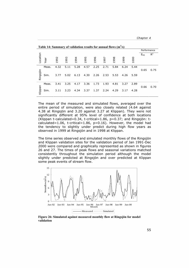
Chapter 4

55

Table 14: Summary of validation results for annual flows (m3/s) Performance

Loca

tion

Yea

r

1992

1993

1994

1995

1996

1997

1998

1999

1000 ENS R2

Meas. 4.32 5.11 5.28 4.57 2.25 2.71 5.84 6.24 5.44

Rin

gsj

ön

Sim. 3.77 5.02 6.13 4.30 2.26 2.53 5.53 4.26 5.59

0.65

0.75

Meas. 3.41 3.25 4.17 3.36 1.73 1.93 4.81 3.27 2.89

Klip

pan

Sim. 3.11 3.23 4.34 3.37 1.37 2.24 4.29 3.17 4.28

0.66

0.70

The mean of the measured and simulated flows, averaged over the entire period of simulation, were also closely related (4.64 against 4.38 at Ringsjön and 3.20 against 3.27 at Klippan). They were not significantly different at 95% level of confidence at both locations (Klippan t-calculated=0.34, t-critical=1.86, p=0.37; and Ringsjön: t-calculated=1.06, t-critical=1.86, p=0.16). However, the model had the tendency to slightly under predict during high flow years as observed in 1999 at Ringsjön and in 1998 at Klippan. The time series observed and simulated monthly flows of the Ringsjön and Klippan validation sites for the validation period of Jan 1991-Dec 2000 were compared and graphically represented as shown in figures 26 and 27. The times of peak flows and seasonal variations matched consistently throughout the simulation period although the model slightly under predicted at Ringsjön and over predicted at Klippan some peak events of stream flow.

0

3

6

9

12

15


Stre

amflo

w (m

3 /s)

Measured Simulated Figure 26: Simulated against measured monthly flow at Ringsjön for model validation

Results

56

0

2

4

6

8

10

12

14


Stre

amflo

w (m

3 /s)

Measured Simulated

Figure 27: Simulated against measured monthly flow at Klippan for model validation

The distribution of predicted monthly stream flows with respect to the measured values were regressed and the 1:1 line fit were plotted as indicated in figures 28 and 29. The results showed that the values were distributed uniformly about the 1:1 line. However, few outliers were observed for the high flows attributed to the under prediction and over prediction of the model at Ringsjön and Klippan, respectively, during the high flow years.

0

3

6

9

12

15

0 3 6 9 12 15Measured flow (m3/s)

Sim

ulat

ed fl

ow (m

3 /s)


Figure 28: Regression and 1:1 line fit plot of observed versus simulated monthly flow for model validation at Ringsjön

Chapter 4

57

0

2

4

6

8

10

12

14

0 2 4 6 8 10 12 14Measured flow (m3/s)

Sim

ulat

ed fl

ow (m

3 /s)


Figure 29: Regression and 1:1 line fit plot of observed versus simulated monthly flow for model validation at Klippan

Although the monthly statistical validation result for Ringsjön had lower ENS and r2 values (0.43 and 0.56), it was still considered satisfactory and the prediction at Klippan was even higher (ENS=0.62 and r2=0.66). The mean of the measured and calculated values at both locations were not significantly different at 95% confidence level since the p-values (0.13 and 0.34) were greater than the α -value of 0.05. Table 15 summarises the statistical results of simulated against measured values on both validation sites. The detailed monthly measured and the corresponding SWAT predicted data are given in appendix A-4.2.

Table 15: Summary of validation results for monthly flows Mean 1-tail t-test, α =0.05 Performance Location Number of

observations Meas. Sim. t-calc t-crit p-value ENS R2

Ringsjön 108 4.65 4.39 1.14 1.66 0.13 0.43 0.56

Klippan 108 3.21 3.27 0.41 1.66 0.34 0.62 0.66

Results

58

4.3 Modelling Nutrient (NO3) Loading of the Rönne Basin

The calibration and validation results for annual and monthly stream flows performed on two sub-basins of the Rönne River Basin were found to be satisfactory indicating that SWAT can be used to model the hydrologic conditions of the entire basin. But the results obtained for nitrate simulation were not so good probably due to the limitations and uncertainties associated with nutrient data, which otherwise would have significantly influenced the model output. Given such prevailing circumstances, therefore, it would be unwise conclusion to associate the poor results due to less performance of SWAT in modelling nitrate within the study area. In fact, the model was successfully used by Grizzetti et al. (2003) to model diffuse emission of nitrogen from the Vantaanjoki watershed in Southern Finland, which has similar watershed properties to the current study area. Therefore, SWAT was applied to assess and show the relative importance of different watershed properties, particularly land uses, in terms of nitrate emission and loading to stream water within the study area based on the calibrated hydrological conditions, but without undermining the possible systematic errors associated in estimating nitrate concentrations in stream water due to the already mentioned uncertainties. Temporal variations due to missing point sources data, for example, are insignificant since they are controlled emissions although the estimated outputs are expected to be far under predicted. Finally, it should be noted that in the subsequent nutrient modelling approach, while the estimated outputs could serve the purpose of analysing relationships between nitrate diffuse emission and different watershed characteristics in relative terms, a further verification of nutrient data is still required in order to use it for management planning in its strictest sense.

4.3.1 NO3 Diffuse Emission Predicting Variables

It was believed that NO3 diffuse emission by surface and subsurface runoff is influenced by watershed properties such as land use/cover types and hence by the area occupied by such land uses. In this research, it was further hypothesised that agricultural land would contribute most to nitrate emission. In order to relate the most predictors of NO3 loading by surface water, a comparison involving the proportion of different land covers and the respective nutrient loading in different sub-basins was performed. The correlation

Chapter 4

59

involved the percentage areas of different land uses in 20 out of the 21 sub-basins and the respective nitrate loading by surface runoff. Sub-basin 17 (the main outlet) was considered as spatial outlier and hence excluded from the analysis because the sub-basin area was too small while it contributed high amount of nitrate load compared to the whole area due to high proportion of urban land within the sub-basin. Table 16 presents the correlation matrix that relates the NO3 loading (NSURQ) and the proportion of land use types from which NO3 was transported by surface runoff during a 10-year simulation period (1991-2000). The cover proportions of different land uses in different sub-basins and the amount of NO3 transported from the respective sub-basins in surface runoff is given in appendix 5.

Table 16: Correlation coefficient between NO3 loading (NSURQ - kg N/ha) and %age field Landuse AGRL FRST PAST RANGB WATR URBN NSURQ AGRL 1 FRST 1 PAST 1 RANGB 1 WATR 1 URBN 1 NSURQ 0.9 -0.7 0.3 -0.5 -0.3 -0.1 1

Note: the comparison involved only nitrate transported in surface runoff (NSURQ).

Nitrate loading was found to be strongly positively correlated to the area occupied by agricultural land (r=0.9) and negatively correlated to the area occupied by forest (r=-0.7). The remaining land use types were less correlated to nitrate leaching compared to agricultural land and forest areas. Nitrate loading was further compared by regressing against the proportion of agricultural and forest covers as shown in figures 30 and 30. The result revealed that agricultural land was strong predictor of nitrate emission (r2 = 0.79) compared to other land use areas suggesting 79% of variation in nitrate loading can be explained by variation in agricultural land proportion within the sub-basin. The positive slope (figure 29) indicates that nitrate loading increases with the increase of agricultural land area and if the watershed was completely free from any agricultural activity, the average nitrate loading from the watershed would be limited to a background value of 0.4 kg N/ha.

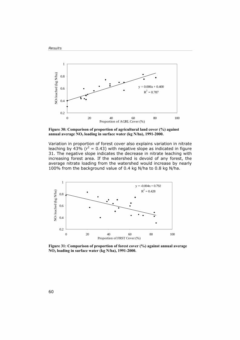
Results

60

y = 0.006x + 0.400R2 = 0.787

0.2

0.4

0.6

0.8

1

0 20 40 60 80 100Proportion of AGRL Cover (%)

NO

3 le

ache

d (k

g N

/ha)

Figure 30: Comparison of proportion of agricultural land cover (%) against annual average NO3 loading in surface water (kg N/ha), 1991-2000.

Variation in proportion of forest cover also explains variation in nitrate leaching by 43% (r2 = 0.43) with negative slope as indicated in figure 31. The negative slope indicates the decrease in nitrate leaching with increasing forest area. If the watershed is devoid of any forest, the average nitrate loading from the watershed would increase by nearly 100% from the background value of 0.4 kg N/ha to 0.8 kg N/ha.

y = -0.004x + 0.792R2 = 0.428

0.2

0.4

0.6

0.8

1

0 20 40 60 80 100Proportion of FRST Cover (%)

NO

3 lea

ched

(kg

N/h

a)

Figure 31: Comparison of proportion of forest cover (%) against annual average NO3 loading in surface water (kg N/ha), 1991-2000.

Chapter 4

61

4.3.2 NO3 Concentration in Stream Water: Spatial Variation

The concentration of NO3 in stream water was also simulated at different sub-basin outlets along the Rönne River to examine the longitudinal spatial trend of stream water quality. The results were plotted from the most upstream sub-basin reach to the most downstream including the main outlet. The simulated results included average annual values for the period 1991-2000 and 1998 wet year as shown in table 17 and figure 32. Longitudinal plot along the main channel at the outlet of the various sub-basins indicated NO3 concentrations increase downstream. The difference between the 10-year average and the 1998 concentrations were high in the downstream areas while there was no significant difference near the upstream sub-basins.

0.0

0.3

0.6

0.9

1.2

1.5

Sb-1

4

Sb-1

2

Sb-1

5

Sb-9

sb-7

Sb-5

Sb-1

8

Sb-3

Sb-1

Sb-1

6

sb-1

7

Subbasin

NO

3-N

(mg/

l)

1991-2000 1998 Figure 32: NO3-N concentration in stream water at different locations along the Rönne River

Table 17: Longitudinal NO3 concentration (mg/l) in stream water along the main channel of Rönne River Sub-basin 14 12 15 9 7 5 18 3 1 16 17

91-00 0.21 0.19 0.15 0.16 0.22 0.31 0.42 0.50 0.49 0.51 0.51 NO3

98 0.23 0.20 0.17 0.22 0.42 0.69 1.02 1.09 1.18 1.34 1.37

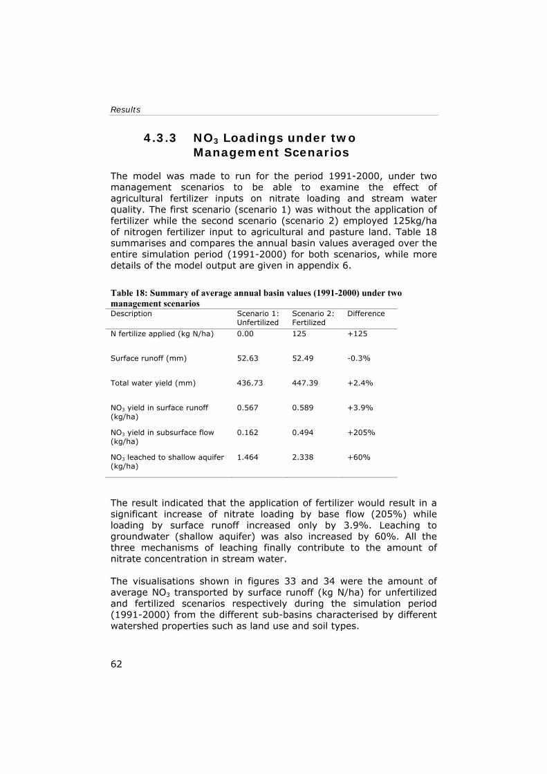
Results

62

4.3.3 NO3 Loadings under two Management Scenarios

The model was made to run for the period 1991-2000, under two management scenarios to be able to examine the effect of agricultural fertilizer inputs on nitrate loading and stream water quality. The first scenario (scenario 1) was without the application of fertilizer while the second scenario (scenario 2) employed 125kg/ha of nitrogen fertilizer input to agricultural and pasture land. Table 18 summarises and compares the annual basin values averaged over the entire simulation period (1991-2000) for both scenarios, while more details of the model output are given in appendix 6.

Table 18: Summary of average annual basin values (1991-2000) under two management scenarios Description Scenario 1:

Unfertilized Scenario 2: Fertilized

Difference

N fertilize applied (kg N/ha) 0.00 125 +125

Surface runoff (mm) 52.63 52.49 -0.3%

Total water yield (mm) 436.73 447.39 +2.4%

NO3 yield in surface runoff (kg/ha)

0.567 0.589 +3.9%

NO3 yield in subsurface flow (kg/ha)

0.162 0.494 +205%

NO3 leached to shallow aquifer (kg/ha)

1.464 2.338 +60%

The result indicated that the application of fertilizer would result in a significant increase of nitrate loading by base flow (205%) while loading by surface runoff increased only by 3.9%. Leaching to groundwater (shallow aquifer) was also increased by 60%. All the three mechanisms of leaching finally contribute to the amount of nitrate concentration in stream water. The visualisations shown in figures 33 and 34 were the amount of average NO3 transported by surface runoff (kg N/ha) for unfertilized and fertilized scenarios respectively during the simulation period (1991-2000) from the different sub-basins characterised by different watershed properties such as land use and soil types.

Chapter 4

63

Figure 33: NO3 loading by surface runoff from different sub-basins, 10-years average (1991-2000) for scenario 1

Figure 34: NO3 loading by surface runoff from different sub-basins, 10-years average (1991-2000) for scenario 2

Results

64

The difference in loading due to fertilization was not as such significant on the visualizations since the significant amount of leaching occurred by subsurface water that can not be visually observed on surfaces. Nevertheless, both maps show that higher density of loading generally occurred from areas dominated by agricultural land, whereas areas to the north mostly occupied by forest showed less loading density. But, few exceptions to such general distributions were observed, for example in sub-basins 2 and 17. Sub-basin 2 is dominated by forest (65%) and sub-basin 17 is occupied by significant proportion of urban land (47%) and forest (40%) whereas, agricultural land occupies only 13%. The least loading rate occurred from sub-basin 4 under both scenarios.

Chapter 5

65

5 Discussion

5.1 Stream Water Flow Modelling

Several hydrologic parameters were adjusted for annual and monthly stream flow calibrations at two locations within the study area. Most of the calibration parameters were based on suggestions of previous SWAT studies (Arnold et al., 2000; Santhi et al., 2005). Since hydrologic conditions are likely to vary considerably between different watersheds, sensitivity analysis is essential in order to identify the most responsive hydrologic conditions for Rönne River basin. Hence, three of the ten input parameters (table 11) used in this study were evaluated for sensitivity that involve the curve number, soil available water capacity, soil evaporation coefficient, groundwater revaporation factor and base flow alpha factor. The result showed that the runoff curve number (CN) was found to be the most sensitive parameter for both surface and base flow, while SOL-AWC and ESCO also influenced both flows though not as significant as CN. These parameters were also found to be sensitive in other previous SWAT studies performed on several watersheds in the U.S.A., for example by (Arnold et al., 2000; Reungsang et al., 2005; Santhi et al., 2005; White and Chaybey, 2005). Similar studies performed in Europe, for example by Grizzetti et al (2003), on the Vantaanjoki watershed in Southern Finland showed that CN was most sensitive in calibrating stream flow. CN is a parameter that adjusts the proportioning between surface runoff and infiltration based on watershed properties such as soil hydrologic group, land use, and antecedent moisture conditions. The sensitivity calculated for flow as a function of average annual values, by varying CN2 from -0.1 to -8 decreases the surface runoff by 38% and 48%, and increases the base flow by 12% and 9% for the calibration sub-basins at Ringsjön and Klippan, respectively. This indicates that surface runoff significantly increases as the curve number increases, while base flow is inversely related to curve number since infiltration rate decreases with increasing surface runoff. The sensitivity also varies between different sub-basins, as observed in this study, due to likely variations in combinations of land use and soil types in different sub-basins. The land use and soil combinations in Klippan (>80% forest and 23 % sand soil) favour more infiltration compared to the upstream sub-basins of Ringsjön characterised by significant proportion of land use and soil types that favour more runoff such as water bodies, agricultural land, urban areas and clay soils with less forest cover.

Discussion

66

ESCO was the second parameter evaluated for sensitivity because it determines the depth distribution for evaporation from the soil (Neitsch et al., 2002) to account for the effect of capillary action, crusting and cracking (Jha et al., 2004). The sensitivity evaluation performed showed that the variation of ESCO value from 1 (no compensation) to 0.1 decreases the surface runoff by 5.4% and 4%, and base flow by 9.5% and 9% for Ringsjön and Klippan sub-basins respectively. This indicates that reduced ESCO value increases the evaporative demand from soil layer making less water available for surface runoff and base flow. The change in base flow at both locations is closely similar may be because only a single soil layer was assumed for the entire basin and hence spatial variation does not account for layer depth variation. SOL-AWC decreases, in both surface and base flow, between 4-5% for an increase of parameter value from 0.001 to 0.05. Increasing the SOL-AWC increases the water holding capacity of the soil that would be more available for plant uptake by reducing the net outflow of water from a sub-basin. On the contrary, decreasing soil water capacity results in less pore space between soil particles and hence less water holding capacity favouring higher runoff and percolation. The calibration and validation of SWAT2000 performed on two locations within the Rönne River Basin produced a satisfactory prediction of stream water flow, for both annual and monthly time steps with slight under predictions of high flows. The mean of the measured and calculated values are not significantly different at 95% confidence level (p<0.05) for all the calibration and validation results. The Nash-Sutcliffe simulation efficiency, ENS, ranges from 0.65 to 0.78 for the annual simulations indicating that the model sufficiently tracked the average annual flows. A coefficient of determination, r2, ranging between 0.70 – 0.79 for annual simulation further confirms the suitability of SWAT to model, especially, the hydrological conditions of the current study area. However, the model performed less efficiently on a monthly basis with computed ENS and r2 values ranging from 0.35 to 0.62 and 0.52 to 0.66 respectively indicating that SWAT is more suitable to model long-term annual effects than short-term monthly variations of basin hydrologic conditions. Although the results obtained can be considered adequate as evaluated graphically and statistically, they showed generally less performance compared to results obtained in previous SWAT studies on similar watersheds. Grizzetti et al. (2003) for example, obtained ENS value of 0.57-0.81 and 0.75-0.81 for daily and monthly time steps respectively during the calibration and validation of SWAT on the Vantaanjoki watershed in Southern Finland. This may indicate

Chapter 5

67

that the present calibration results could be further improved by verifying the model input data such as land use, soil and climate since these dataset might had been greatly generalised somewhat overlooking the spatial variability of basin characteristics.

5.2 Nutrient (NO3) Load Modelling

Although the simulated time-series plot tends to follow the temporal variations of the observed data (figure 22), the calibration result for the selected nutrient (NO3-N) was poor with negative Nash-Sutcliffe prediction efficiency. All parameters suggested in various literatures for NO3 calibration (Neitsch et al., 2002; Santhi et al., 2005; White and Chaybey, 2005), such as SOL-NO3, BIOMIX, NPERCO, RSDCO and fertilizer application rates were rigorously adjusted to effectively simulate the measured data, but the result remained far under predicted without significant improvement. The nitrate percolation coefficient (NPERCO) was found to be the only sensitive parameter that significantly changes NO3 concentration (>300%) with a parameter variation from 0 to 1. It adjusts the proportion of concentration of nitrate between surface runoff and percolating water (Neitsch et al., 2002) in such a way that higher value of NPERCO increases NO3 transport in surface water and hence concentration in stream water. The consistent under prediction of the model in calibrating NO3 is not surprising since nutrient related model data input was not exhaustively verified due to lack of information. One of such data input involves point sources from waste water treatment plants (WWTPs) located within the basin that is believed to greatly influence the model output. Several point sources from WWTPs are found in the study area and two of them are located within the sub-basin selected for calibration for which point discharge data could not be available to include in this particular study. A SWAT study in Germany (Pohlert et al., 2005) demonstrated that the contribution of point source pollution, especially during low flow periods in summer can reach up to 90% of the total nitrate load at the outlet. This implies the significance of point sources in altering the under predicted nitrate concentration in stream in this study although the point source contribution proportion may differ from that of Germany depending on local conditions. Management data, such as timing, type and amount of fertilizer applications, crop types and growing seasons are also closely related to nutrient loading. The management data used in this study were

Discussion

68

solely based on available literature sources for the whole Sweden, regional in nature, which are not watershed-specific to exceptionally represent the study area that may lead to additional discrepancies. However, the discrepancy due to such management data may not be significant as discussed by Grizzetti et al. (2003) since other watershed characteristics such as soil properties are more important than crop and management parameters in model predictions. Uncertainties associated with NO3 concentration were further examined by comparing the time-series measured concentration data against measured flow to observe the seasonal behaviour if variation in NO3 concentration can be explained by seasonal stream flow variation as indicated in figure 23. The result showed a negative correlation with very low coefficient of determination (r2 = 0.02) suggesting that variation in NO3 concentration could not be explained by the variation in discharge. This may be partially true since other factors such as soil types and land uses also control NO3 exports from sub-basins. However, this is in disagreement with previous works performed in other watersheds, for example, in Belgium (Van Herpe and De Troch, 2000) and several other researched works cited there-in. Van Herpe and De Troch (2000) reported positive correlations, and on average 32% (r2=0.32) of the variation in NO3 concentration was explained by the variation in discharge volume with out any significant negative correlations between discharge and concentration. The low value of r2 in this study may, therefore, be attributed to the likely error associated to the sampling and analysis procedures for NO3 concentration. This can be further explained by the fact that the measured data were not continuous daily discharge data (only grab samples) so that the possibility of low precision and less representativeness of the data may not be ruled out. Santhi et al. (2005) underscored the necessity of continuous collection of monitoring data for adequate calibration and validation of SWAT model. Uncertainties are also likely due to the model itself since some nutrient related processes are not considered to fully account for nitrogen balances. The contribution of Nitrous oxide (N2O), for example, as a possible pathway for N-losses is not included into the model. Therefore, further verification of the N-balances for the sub-basin, by attempting to estimate the overall N-budgets, i.e. inputs, exports and transformations, may help minimize such uncertainties. Groundwater quality data in terms of N-levels, for example, could be

Chapter 5

69

used to verify the N- leaching to groundwater and the contributions expected back from the groundwater store.

5.3 Scenario Analysis

Obviously, the uncertainty associated with nitrate modelling due to the limitations discussed above is a drawback for comprehensive scenario analysis that would enable the estimation and study of nitrate loading from different sub-basins and concentration in stream water since the resulting model outputs are greatly influenced by the quality of input data. However, different scenarios could be examined in relative terms so that the spatial and temporal variations of nutrient in relation to different watershed attributes such as land use, soil types, topographic feature, and management scenarios would be investigated. The first scenario analysis was introduced to scrutinize the relationship between different land use types and NO3 loading by surface water that finally makes its way to stream waters. NO3 (kg N) transported by surface water from the various land covers was statistically compared to the field percentages and the result showed the amount of nitrate leached positively correlated to the percentage area occupied by agricultural land (r= 0.9, r2= 0.79). A similar strong correlation was obtained (Grizzetti et al., 2003) in the Vantaanjoki basin of Southern Finland by considering total nitrogen loads and agricultural surface of the drained catchments. This analysis also indicated the positive correlation between in-stream NO3 concentration (mg/l) and proportion of arable land although the correlation coefficient obtained (r= 0.37) is weaker than that of the NO3 load (r=0.90). The lower correlation coefficient for nitrate concentration compared to loading may be attributed to additional factors that influence nutrient concentrations such as in-stream nutrient processes that undergo different transformations. Nonetheless, both nitrate transport in surface water (kg N) and concentration in stream water (mg/l) are well explained by agricultural land, which could be attributed to the application of fertilizers. Similarly, Grizzetti et al. (2003) discussed the well predictability of nutrient load by agricultural surface even without specifying crop type. Previous scenarios modelled in the study area (Arheimer et al., 2004) also suggested that changing agricultural practices is the most effective way to reduce nitrogen transport from land to lakes and the sea indicating that nutrient emission is well predicted by agricultural land.

Discussion

70

This study also showed diffuse emissions are lower for other land use types and particularly negatively correlated with percentage of forest cover (r = -0.7). A statistical analysis performed on a watershed in Belgium (Van Herpe and De Troch, 2000) showed analogous results whereby higher percentages of forested area resulted in lower NO3 concentrations. This indicates that NO3 emission to surface and subsurface waters decreases with increasing forest surface mainly due to the increased demand of plant nitrogen uptake as indicated by the nitrogen cycle (figure 9) and SWAT nitrogen pool (figure 10). The CN associated to forest cover is also believed to influence, at least, nitrate transport in surface runoff by increasing infiltration. The second scenario studied was the spatial variation of NO3 concentration in stream water at the outlet of various sub-basins along the Rönne River. The longitudinal pattern along the main stream, as observed in figure 32 and table 17, shows that the concentration of NO3 increases downstream. This is not an unexpected trend, since the volume of water that carries nutrients from sub-basins increases in the downstream direction. This can be further explained by comparing the ten year average and the 1998 wet year NO3 concentration as indicated in figure 32. The difference between the two in the first few upstream sub-basins is practically insignificant since the volume of water and sub-basin area contributing to NO3 loading are small. But it becomes significant in the downstream areas as the volume of water for 1998 rises above the ten year average due to large draining area to carry more nutrients. The downstream increase of nitrate concentration may be explained not only by the enhanced volume of water (hydrologic regime) responsible for transporting but also by the spatial distribution of basin characteristics such as topography, soil type and land use. In this study, it was hypothesised that arable land is the major source of nutrient concentrations in stream water. This can be justified by comparing the increasing nitrate concentration (figure 32 and table 17) corresponding to the downstream intensification of agricultural activity along the main channel (figure 13 and appendix 2). Similar phenomenon was observed and discussed (Van Herpe and De Troch, 2000) in Belgium where the influence of anthropological land use activities (increasing arable land) was reflected in the longitudinal NO3 concentration pattern along the main stream with positive correlation. Finally, two different management scenarios for fertilizer application were considered in order to evaluate the effects on NO3 loading. Scenario 1 was without the application of fertilizer while scenario 2 considers 125kg/ha of nitrogen fertilizer input to agricultural and

Chapter 5

71

pasture lands represented by spring barley. The simulation result averaged over 10 years showed an annual increase of NO3 loading by 4%, 267% and 63% to surface water, subsurface water and shallow aquifer, respectively under fertilized scenario (table 18). The spatial distribution of NO3 leaching exhibits similar densities for both scenarios except slight increase observed after fertilization (cf. figures 33 and 34). Generally, most of the leaching is related to agricultural land as observed from the simulation visualised in figures 33 and 34) and this has been statistically confirmed as explained above. The least rate of leaching occurred in sub-basin 4 under both scenarios. Sub-basin 4 is covered by forest and totally devoid of agricultural land. However, exceptions are also observed in this simulation whereby high density of loading is related to other areas different from agricultural land. The high rate of loading from sub-basin 2, for example may not be explained by agricultural land since the proportion of forest cover is much higher (65%) than agricultural land surface (35%). This indicates that other watershed characteristics may control the NO3 loading within the basin. One of such factors could be the effect of topographic feature that controls the rate of surface runoff and hence the rate of nutrient leaching. This has been discussed by Van Herpe and De Troch (2000) that steep slopes generate more surface runoff and less infiltration compared with gentle or flat slopes. Although such hydrologic process has a diluting effect on stream water NO3 concentrations due to greater volume of water, on the other hand it carries a considerable amount of nutrients from land surface causing huge loss of NO3 from sub-basins. This is a possible circumstance in sub-basin 2 mainly covered by forest but generating high nitrate export. The steepest slope is in fact found in sub-basin 2 with mean standard deviation of elevation being the highest (59) compared to the rest of sub-basins, only closely followed by sub-basin 21 with standard deviation of 55 (appendix 1) for which surface leaching is also high. This indicates that the sub-basins generate high rate of runoff and hence high nitrate export in surface water influenced by the topographic feature as observed in sub-basins 2 and 21.

73

6 Conclusion

The hydrologic conditions and nitrate loading from land to stream water within the Rönne River basin were modelled using SWAT hydrologic and water quality model. The model calibration and validation procedures for stream flow confirmed that the model adequately simulates the hydrologic regime of the study area. The simulated stream flow was found to be sensitive to variations in curve number, the soil evaporation coefficient and soil available water capacity that the selection of values of the parameters can significantly change the predicted stream flow results. The calibration result for nitrate concentration in stream water was rather poor probably attributed to the scantiness of information and input data used for the model. Nevertheless, the calibrated model for hydrologic conditions was used to assess the relationships between different watershed attributes and nitrate losses within the watershed. The simulation result over the period of 10-years (1991-2000) showed that nitrate loading by surface water is strongly positively correlated to the percentage area occupied by agricultural land and negatively correlated to the area occupied by forest. Nitrate concentration in stream water is also correlated and spatially varied with intensively cultivated agricultural land longitudinally along the main channel of the Rönne River. There is also an indication that nutrient loading could be influenced by topographic features, steeper slopes being responsible for enhanced transport of nitrate by surface runoff. Generally, agricultural land is a strong predictor of nitrate emission from land that 79% of variation in nitrate loading can be explained by variation in agricultural land cover. The loading in surface water is also influenced by change in forested area with r2 value of 0.43. Therefore, changing agricultural practice and increasing forest area will effectively reduce nitrate leaching to surface waters within the Rönne basin and the nearby coastal North Sea. Finally, this study showed that SWAT model is a powerful tool that can be used for hydrological analysis of Rönne River basin, especially when dealing with water balance and quantity aspects. However, further nutrient data verification is essential for a reliable estimation of nitrate load values, related to water quality problems, to help effective management planning and decision-making processes within the watershed.

References

75

References

Arheimer, B., L. Andersson, M. Larsson, G. Lindström, J. Olsson and B. C. Pers, 2004. Modelling diffuse nutrient flow in eutrophication control scenarios. Water Science and Technology, 49(3): 37-45.

Arnold, J.G., Muttiah, R.S., Srinivasan, R. and Allen, P.M., 2000. Regional Estimating of Baseflow and Groundwater Recharge in the Mississippi River Basin. Journal of Hydrology(227): 21-44.

Arnold, J.G., Srinivasan, R., Muttiah, R.S. and Williams, J.R., 1998. Large area hydrologic modelling and assessment. Part I: Model development. Journal of the American Water Resources Association, 34(1): 73-89.

Bhuyan, S.J., Koelliker, J.K., Marzen, L.J. and Harrington, J.A., Jr., 2003. An integrated approach for water quality assessment of a Kansas watershed. Environmental Modelling and Software, 18: 473-484.

Borah, D.K. and Bera, M., 2003. Watershed-Scale Hydrologic and Nonpoint-Source Pollution Models: Review of Mathematical Bases. American Society of Agricultural Engineers, 46(6): 1553-1566.

Chaplot, V., 2005. Impact of DEM mesh size and soil map scale on SWAT runoff, sediment, and NO3-N loads predictions. Journal of Hydrology, 312: 207-222.

Chapman, D. (Editor), 1996. Water Quality Assessment. E & FN Spon, London and New York, 626 pp.

Daniel, E., 1978. Description of the Quaternary map: Hoganas No/Helsingborg NV, Sveriges Geologiska Undersokning, Stockholm.

De Wit, M., 1999. Nutrient Fluxes in the Rhine and Elbe Basins. PhD Thesis, Universiteit Utrecht, Utrecht, 163 pp.

DiLuzio, D., Srinivasan, R., Arnold J.G. and Neitsch S.L., 2002. ArcView Interface for SWAT2000. User's Guide. BRC Report 02-03, Texas Water Resources Institute, College Station, Texas.

EEA, 1998a. Environment in European Union at the turn of the century. Appendix to the summary, facts and findings per environmental issues, European Environment Agency, Copenhagen.

EEA, 2000. Corine land cover 2000 vector by country (CLC2000). European Environment Agency, On-line document, URL: http://dataservice.eea.eu.int/dataservice, Access date: 06 Nov 2005, Copenhagen.

References

76

EEA, 2001. Nitrate concentrations in rivers. European Environment Agency: On-line document, URL: http://themes.eea.eu.int, Access date: 01 Dec 2005.

EEA, 2003. Status of Europe's water. 1/2003, European Environment Agency, Copenhagen.

Ekologgruppen, 2000. Wetlands in Agricultural Areas, Lunds Kommun, Lund, Sweden.

Engman, E.T., 2002. Remote sensing based continuous hydrologic modelling. Advances in Space Research, 4(11): 201-209.

Eriksson, J., Andersson, A. and Andersson, R., 1997. Current status of Swedish arable soils: Summary, Online document, URL: http://www-umea.slu.se, Access date 20 Nov 2005.

Euroharp, 2005. Towards European Harmonised Procedures for Quantification of Nutrient Losses from Diffuse Sources. Euroharp.org, On-line document, URL: http://euroharp.org, Access date: 10 Sep 2005.

European Commission, 2000. Directive 2000/60/EC of the European Parliament and of the Council: establishing a framework for community action in the field of water policy. Official Journal of the European Communities(L327): 1-72.

European Commission, 2002. Implementation of Council Directive 91/676/EEC concerning the protection of waters against pollution caused by nitrates from agricultural sources. European Commission, Luxembourg.

European Commission, 2003. Water for Life: International cooperation from knowledge to action. European Commission, Luxembourg.

European Community, 1991. Council Directive 91/676/EEC concerning the protection of waters against pollution caused by nitrates from agricultural sources. Off. J. L 375.

Galloway, J.N., 1998. The global nitrogen cycle: changes and consequences. Environmental Pollution, 102(SI(1998)): 15-24.

Grizzetti, B., Bouraoui, F., Granlund, K., Rekolainen, S. and Bidoglio, G., 2003. Modelling diffuse emission and retention of nutrients in the Vantaanjoki watershed (Finland) using the SWAT model. Ecological Modelling, 169: 25-38.

Gustafsson, O., 1992. Grundvattenkartor: Beskrivning till hydrogeologiska kartan Hoganas NO/Helsingborg NV, SGU, Uppsala.

Hijmans, R.J., S.E. Cameron, J.L. Parra, Jones, P.G. and A. Jarvis, 2004. The WorldClim interpolated global terrestrial climate surfaces. Version 1.3. Available at http://biogeo.berkeley.edu/, Access date: 10 Dec 2005.

References

77

Howarth, R.W. (Editor), 1996. Nitrogen cycling in the North Atlantic Ocean and its watersheds. Kluwer, Dordrecht, 304 pp.

Jayakrishnan, R., Srinivasan, R., Santhi, C. and J.G., A., 2005. Advances in the application of the SWAT model for water resources management. HYDROLOGICAL PROCESSES, 19(2005): 749-762.

Jha, M., Gassman, P.W., Sechi, S., Gu, R. and Arnold, J., 2004. Effect of Watershed Subdivision on SWAT Flow, Sediment, and Nutrient Predictions. Journal of the American Water Resources Association, 40(3): 811-825.

Jonsson, H., Larsson, M., Martensson, K. and Hoffmann, M., 2002. SOILNDB: a decision support tool for assessing nitrogen leaching losses from arable land. Environmental Modelling & Software, 17: 505-517.

Kerle, N., Janssen, L.L.F. and Huurneman, G.C. (Editors), 2004. Principles of Remote Sensing. (ITC Educational Textbook Series; 2), Third edition, Enschede.

Khairy, W.M., Hannoura, A.P., Cothren, G.M. and McCorquodale, A., 2000. Application of information systems in modelling of nonpoint pollution, 4th International Conference on Integrating GIS and Environmental Modelling (GIS/EM4): Problems, Prospects, and Research Needs., Banff, Alberta, Canada, September 2-8, 2000.

Krantz, D. and Kifferstein, B., 2005. Water Pollution and Society. On-line document, URL: - http://www.umich.edu : Access date: 30 Nov 2005.

Matejicek, L., Benesova, L. and Tonika, J., 2003. Ecological modelling of nitrate pollution in small river basins by spreadsheets and GIS. Ecological Modelling, 170(2-3): 245-263.

Matson, P.A., Parton, W.J., Power, A.G. and Swift, M.J., 1997. Agricultural Intensification and Ecosystem Properties. Science, 277(5325): 504 - 509.

McDonald, A. and Kay, D., 1988. Water Resources: Issues and Strategies. Longman Group UK Ltd, Essex, 284 pp.

Muller, E., Decamps, H. and Dobson, M., 1993. Contribution of Space Remote-Sensing to River Studies. Freshwater Biology, 29(2): 301-312.

Nash, J.E. and Sutcliffe, J.V., 1970. River flow forecasting through conceptual models. Part 1-A: Discussion of principles. Journal of Hydrology, 10(3): 282-290.

Neitsch, S.L., Arnold, J.G., Kiniry, J.R., Williams, J.R. and King, K.W., 2002. Soil and Water Assessment Tool Theoretical Documentation. Version 2000, Texas Water Resources Institute, College Station, Texas.

References

78

Norling, E. and Wikman, H., 1990. Description of the map of solid rocks: Hoganas No/Helsingborg NV, Sveriges Geologiska Undersokning, Uppsala.

Pidwirny, M., 2005. Fundamentals of Physical Geography. Online document, URL: http://www.physicalgeography.net, Access date 60 Dec 2005.

Pohlert, T., J. A. Huisman, L. Breuer and Frede, H.-G., 2005. Modelling of point and non-point source pollution of nitrate with SWAT in the river Dill, Germany. Advances in Geosciences, 5: 7–12.

PVCoolBuild, 2003. Solar radiation data for PVCoolBuild, Online document, URL: http://www.pvcoolbuild.com, Access date 60 Dec 2005.

Rao, K. and Kumar, D., 2004. Spatial decision support system for watershed management. Water Resources Management, 18(5): 407-423.

Reungsang, P. et al., 2005. Calibration and Validation of SWAT for the Upper Maquoketa River Watershed. Center for Agricultural and Rural Development, Iowa State University. Online document, URL: www.card.iastate.edu, Access date: 05 Jan 2006.

Romanowicz, A.A., Vanclooster, M., Rounsevell, M. and La Junesse, I., 2005. Sensitivity of the SWAT model to the soil and land use data parameterisation: a case study in the Thyle catchment, Belgium. Ecological Modelling, 1876: 27-39.

Santhi, C., Srinivasan, R., Arnold, J.G. and Williams, J.R., 2005. A modeling approach to evaluate the impacts of water quality management plans implemented in a watershed in Texas. Environmental Modelling & Software, article in press.

Saxton, K.E., 2003. Soil Water Characteristics: Hydraulic Properties Calculator, Online document, URL: http://www.bsyse.wsu.edu/saxton/soilwater, Access date: 20 Dec 2005.

Scharmer, K. and Greif, J., 2000. The European Solar Radiation Atlas. Database and exploitation software, Vol. 2. Presses de l'Ecole des Mines, Paris, France.

STOWA/RIZA, 1999. Smooth Modelling in Water Management, Good Modelling Practice Handbook; STOWA report 99-05. Dutch Dept. of Public Works, Institute for Inland Water Management and Waste Water Treatment, report 99.036.

Tetra Tech Inc., 2004. Appendix C: Application of the Soil Water Assessment Tool (SWAT) to the Wabash River Watershed, Ohio, U.S. Environmental Protection Agency Region 5, Watersheds and Wetlands Branch, Cleveland.

Tolson, B.A. and Shoemaker, C.A., 2004. Watershed Modelling of the Cannonville Basin using SWAT2000: Model development,

References

79

calibration and validation for the prediction of flow, sediment and phosphorus transport to the Cannonsville Reservoir. Version 1.0. Technical Report, School of Civil and Environmental Engineering, Cornell University. Online document, URL: www.brc.tamus.edu, Access date: 16 Sep 05, NY, pp. 159.

Tripathi, M.P., Panda, R.K. and Raghuwanshi, N.S., 2003. Identification and Prioritization of Critical Sub-watersheds for Soil Conservation Management using the SWAT Model. Biosystems Engineering, 85(3): 365-379.

UNEP/DEWA-Europe, 2004. Freshwater in Europe: Facts, Figures and Maps, United Nations Environment Programme, Geneva.

University of Maryland, 2005. Global Land Cover Facility, Online document, Available at: http://glcf.umiacs.umd.edu, Access date: 15 Aug 05. University of Maryland, Maryland.

Van Herpe, Y. and De Troch, P.A., 2000. Spatial and temporal variations in surface water nitrate concentrations in a mixed land use catchment under humid temperature climatic conditions. HYDRLOGICAL PROCESSES, 14(14): 2439-2455.

VASTRA, 2005. Description of the pilot area - the Rönne River catchment area. On-line document, URL: http://www.vastra.org/ronnea/ronnea.asp : Access date: 29 June 2005.

Vitousek, P.M. et al., 1997. Human Alteration of the Global Nitrogen Cycle: Sources and Consequences. Ecological Applications, 7(7): 737–750.

White, D.A., Smith, R.A., Price, C.V., Alexander, R.B. and Robinson, K.W., 1992. A Spatial Model to Aggregate Point-source and Nonpoint-source Water-quality Data for Large Areas. Computers and Geosciences, 18(8): 1055-1073.

White, K.L. and Chaybey, I., 2005. Sensitivity Analysis, Calibration, and Validations for a Multisite and Multivariable SWAT Model. JOURNAL OF THE AMERICAN WATER RESOURCES ASSOCIATION (JAWRA), 41(5): 1077-1089.

Wolf, J., Beusen, A.H.W., Groenendijk, P., Kroon, T., Rötter, R. and van Zeijts, H., 2003. An integrated modelling system SOTNE for calculating nutrient emissions from agriculture in the Netherlands. Environmental Modelling and Software, 18: 597-617.

Appendices

81

Appendices

Appendix 1: Topographic statistical summary

A-1.1 Elevation report for the watershed

Min. Elevation: 0 Max. Elevation: 220.333 Mean. Elevation: 89.87 Std. Deviation: 41.1029 ----------------------------------------------------------------------------

A-1.2 Elevation report for each sub-basin

Sub-basin # 1 Min. Elevation: 0.366667 Max. Elevation: 77.6444 Mean. Elevation: 27.1339 Std. Deviation: 14.4413 ------------------------------------- Sub-basin # 2 Min. Elevation: 4.43333 Max. Elevation: 206.489 Mean. Elevation: 115.026 Std. Deviation: 59.0218 ------------------------------------- Sub-basin # 3 Min. Elevation: 5.26667 Max. Elevation: 204.089 Mean. Elevation: 68.7082 Std. Deviation: 47.1641 ------------------------------------- Sub-basin # 4 Min. Elevation: 38.7778 Max. Elevation: 150.617 Mean. Elevation: 95.448 Std. Deviation: 22.3323 ------------------------------------- Sub-basin # 5 Min. Elevation: 37.6444 Max. Elevation: 117.467 Mean. Elevation: 66.207

Sub-basin # 12 Min. Elevation: 53.5333 Max. Elevation: 159.567 Mean. Elevation: 82.6792 Std. Deviation: 27.0774 ------------------------------------- Sub-basin # 13 Min. Elevation: 77.1222 Max. Elevation: 186.8 Mean. Elevation: 146.521 Std. Deviation: 20.3408 ------------------------------------- Sub-basin # 14 Min. Elevation: 77.3667 Max. Elevation: 187.9 Mean. Elevation: 147.044 Std. Deviation: 22.7102 ------------------------------------- Sub-basin # 15 Min. Elevation: 53.5889 Max. Elevation: 113.856 Mean. Elevation: 65.0945 Std. Deviation: 14.7067 ------------------------------------- Sub-basin # 16 Min. Elevation: 0 Max. Elevation: 127.089 Mean. Elevation: 41.61

Appendices

82

Std. Deviation: 18.9847 ------------------------------------- Sub-basin # 6 Min. Elevation: 42.6889 Max. Elevation: 168.8 Mean. Elevation: 84.5067 Std. Deviation: 31.373 ------------------------------------- Sub-basin # 7 Min. Elevation: 42 Max. Elevation: 167.078 Mean. Elevation: 90.5339 Std. Deviation: 27.9726 – – --------------------------------- Sub-basin # 8 Min. Elevation: 44.8889 Max. Elevation: 172.611 Mean. Elevation: 108.967 Std. Deviation: 23.5944 ------------------------------------- Sub-basin # 9 Min. Elevation: 42.8889 Max. Elevation: 127 Mean. Elevation: 79.5981 Std. Deviation: 17.6689 ------------------------------------- Sub-basin # 10 Min. Elevation: 53.3889 Max. Elevation: 169.256 Mean. Elevation: 83.7107 Std. Deviation: 23.6541 ------------------------------------- Sub-basin # 11 Min. Elevation: 53.4889 Max. Elevation: 175.48 Mean. Elevation: 109.173 Std. Deviation: 27.6952 -------------------------------------

Std. Deviation: 29.6787 ------------------------------------- Sub-basin # 17 Min. Elevation: 0.0333333 Max. Elevation: 37.9556 Mean. Elevation: 11.0494 Std. Deviation: 9.22288 ------------------------------------- Sub-basin # 18 Min. Elevation: 34.3889 Max. Elevation: 93.7556 Mean. Elevation: 54.6465 Std. Deviation: 12.2109 ------------------------------------- Sub-basin # 19 Min. Elevation: 11.5444 Max. Elevation: 149.722 Mean. Elevation: 93.8542 Std. Deviation: 24.4071 ------------------------------------- Sub-basin # 20 Min. Elevation: 2.04444 Max. Elevation: 175.525 Mean. Elevation: 96.9643 Std. Deviation: 28.6877 ------------------------------------- Sub-basin # 21 Min. Elevation: 6.94444 Max. Elevation: 220.333 Mean. Elevation: 93.3582 Std. Deviation: 54.5715

Appendices

83

Appendix 2: Landsat image and classified land use map

Landsat ETM+ 7 image of the study area, acquisition date: 03 Aug 1999, with display colour bands: R=7, G=5, and B=4. The resulting classified land use map was based on semi-supervised image classification method.

Appendices

84

Appendix 3: SWAT main output files

Three main SWAT output files: the HRU file (.sbs), the main channel or reach out put file (.rch) and the sub-basin file (.bsb). In this study, (.rch) and (.bsb) were widely used for data analysis.

Appendix 4: Calibration and validation data

A-4.1: Flow calibration data

Table showing measured stream flow (monthly daily average) and the corresponding SWAT predicted values for two locations within the watershed. The calibration was performed for a period of 10-years (Jan 81-Dec 90).

Ringsjön KlippanDate Meas. (m3/s)

Sim. (m3/s)

Meas. (m3/s)

Sim. (m3/s)

Jan-81 15.85 0.05 6.22 0.00Feb-81 15.70 0.09 8.08 0.26

Appendices

85

Mar-81 12.21 1.89 8.60 1.60Apr-81 5.79 1.74 2.40 2.15May-81 1.32 0.66 1.30 0.88Jun-81 2.22 1.40 1.66 0.41Jul-81 2.23 1.14 1.60 0.52

Aug-81 1.71 0.79 0.82 0.49Sep-81 1.73 0.90 0.56 0.32Oct-81 1.73 6.51 5.07 4.43Nov-81 6.78 11.86 10.19 9.23Dec-81 10.44 10.40 4.14 8.48Jan-82 8.88 8.41 2.47 5.87Feb-82 2.18 5.65 3.95 4.35Mar-82 9.94 6.68 8.12 4.74Apr-82 3.92 3.16 2.56 2.53May-82 2.07 1.51 2.91 1.83Jun-82 2.14 0.94 1.51 0.82Jul-82 1.45 0.16 0.61 0.34



Aug-84 2.99 1.10 0.72 0.52Sep-84 2.36 4.26 2.00 1.61Oct-84 3.19 6.54 5.23 4.92Nov-84 4.70 5.72 3.55 4.61

Appendices

86

Dec-84 5.58 5.31 3.62 4.26Jan-85 5.08 4.03 1.43 2.90Feb-85 3.29 7.49 3.24 6.37Mar-85 0.69 3.95 3.25 3.08Apr-85 9.21 4.59 7.93 3.69May-85 7.85 2.52 4.23 2.85Jun-85 2.14 1.48 1.49 1.25Jul-85 1.55 0.73 0.90 0.53




Aug-88 2.55 0.63 1.76 1.98

Appendices

87

Sep-88 3.27 2.13 2.53 1.60Oct-88 4.13 5.96 4.12 4.32Nov-88 5.87 4.48 2.80 3.23Dec-88 2.11 6.62 5.97 4.96Jan-89 8.12 4.72 6.37 4.06Feb-89 3.26 4.23 4.68 3.61Mar-89 4.05 6.18 5.71 4.82Apr-89 4.24 3.87 4.58 3.08May-89 1.54 1.05 2.31 1.35Jun-89 1.91 0.31 1.43 0.54Jul-89 2.12 0.14 0.50 0.28


Aug-90 2.70 0.22 1.09 0.62Sep-90 2.56 2.12 2.03 0.49Oct-90 3.06 3.85 2.09 3.79Nov-90 3.18 4.68 3.68 3.44Dec-90 4.69 4.76 3.25 3.48

A-4.2: Flow validation data

Table showing measured stream flow (monthly daily average) and the corresponding SWAT predicted values for two locations within the watershed. The validation was performed for a period of 10-years (Jan 1991-Dec 2000).

Ringsjön KlippanDate Meas. (m3/s)

Sim. (m3/s)

Meas. (m3/s)

Sim. (m3/s)

Jan-91 3.95 0.06 5.35 0.00Feb-91 6.55 0.03 3.05 0.00Mar-91 3.53 0.02 3.40 0.01Apr-91 2.82 0.03 2.25 0.01

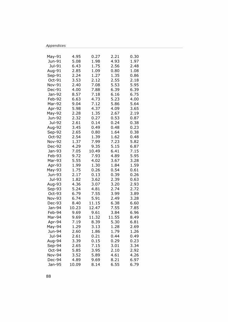
Appendices

88

May-91 4.95 0.27 2.21 0.30Jun-91 5.08 1.98 4.93 1.97Jul-91 6.43 1.75 2.56 2.48




Aug-94 3.39 0.15 0.29 0.23Sep-94 2.65 7.15 3.01 3.34Oct-94 5.85 3.95 2.10 2.92Nov-94 3.52 5.89 4.61 4.26Dec-94 4.89 9.69 8.21 6.97Jan-95 10.09 8.14 6.55 6.79

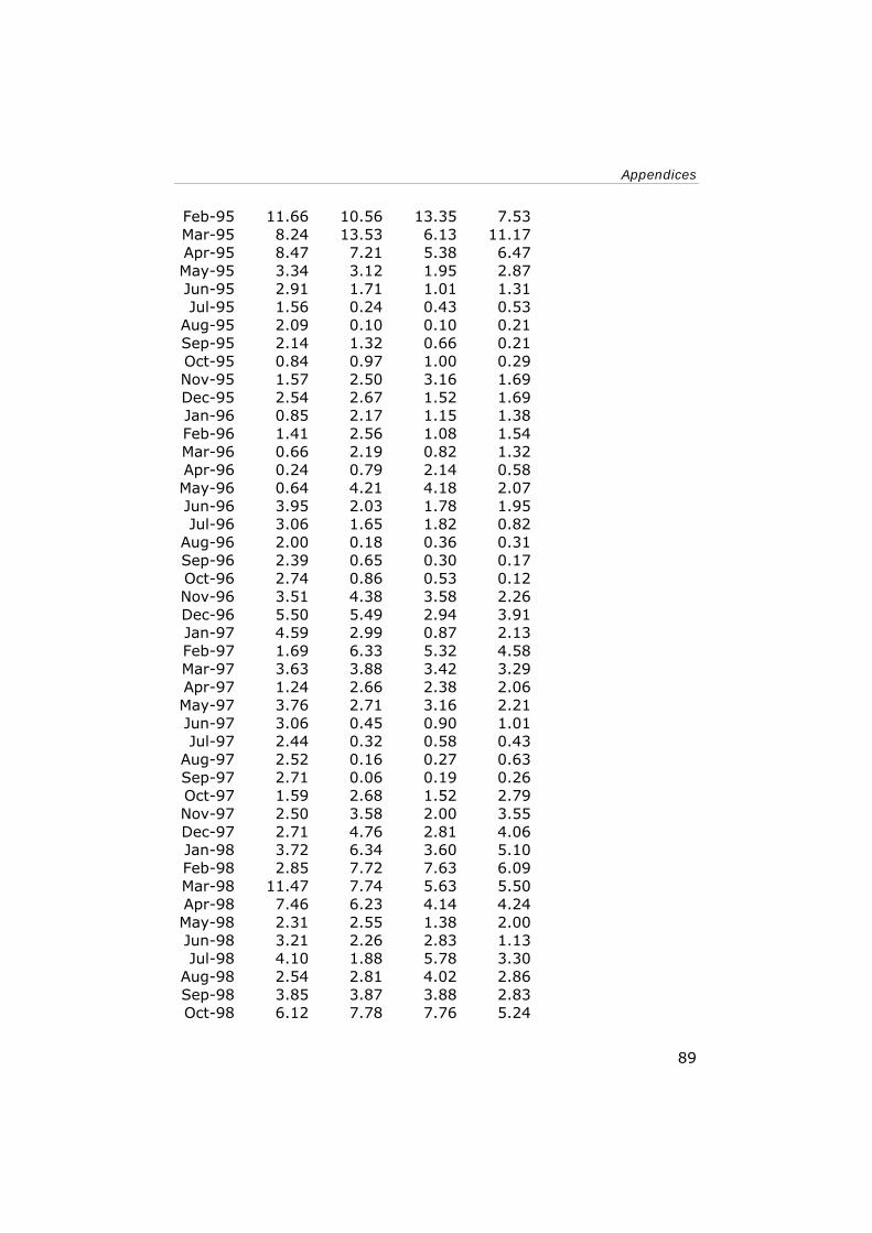
Appendices

89

Feb-95 11.66 10.56 13.35 7.53Mar-95 8.24 13.53 6.13 11.17Apr-95 8.47 7.21 5.38 6.47May-95 3.34 3.12 1.95 2.87Jun-95 2.91 1.71 1.01 1.31Jul-95 1.56 0.24 0.43 0.53




Aug-98 2.54 2.81 4.02 2.86Sep-98 3.85 3.87 3.88 2.83Oct-98 6.12 7.78 7.76 5.24

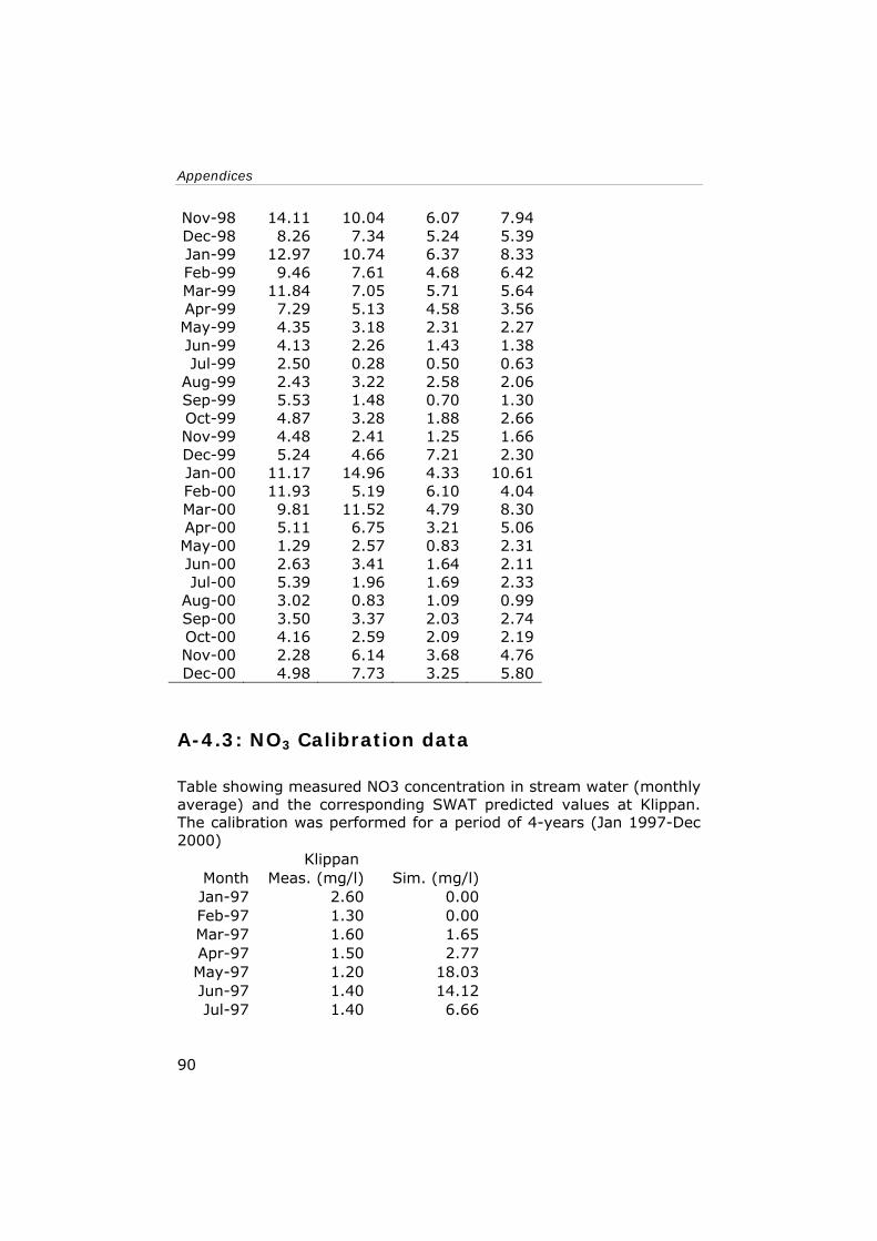
Appendices

90

Nov-98 14.11 10.04 6.07 7.94Dec-98 8.26 7.34 5.24 5.39Jan-99 12.97 10.74 6.37 8.33Feb-99 9.46 7.61 4.68 6.42Mar-99 11.84 7.05 5.71 5.64Apr-99 7.29 5.13 4.58 3.56May-99 4.35 3.18 2.31 2.27Jun-99 4.13 2.26 1.43 1.38Jul-99 2.50 0.28 0.50 0.63


Aug-00 3.02 0.83 1.09 0.99Sep-00 3.50 3.37 2.03 2.74Oct-00 4.16 2.59 2.09 2.19Nov-00 2.28 6.14 3.68 4.76Dec-00 4.98 7.73 3.25 5.80

A-4.3: NO3 Calibration data

Table showing measured NO3 concentration in stream water (monthly average) and the corresponding SWAT predicted values at Klippan. The calibration was performed for a period of 4-years (Jan 1997-Dec 2000)

Klippan Month Meas. (mg/l) Sim. (mg/l)Jan-97 2.60 0.00Feb-97 1.30 0.00Mar-97 1.60 1.65Apr-97 1.50 2.77May-97 1.20 18.03Jun-97 1.40 14.12Jul-97 1.40 6.66

Appendices

91

Aug-97 1.80 1.61Sep-97 1.40 1.01Oct-97 1.80 0.13Nov-97 1.20 0.05Dec-97 1.50 0.20Jan-98 1.80 0.06Feb-98 1.90 0.07Mar-98 1.70 0.18Apr-98 1.10 0.03May-98 1.40 0.61Jun-98 1.50 0.83Jul-98 0.78 0.14



Aug-00 1.10 0.21Sep-00 0.86 0.29Oct-00 0.80 0.07Nov-00 0.78 0.04Dec-00 1.00 0.12

Appendices

92

Appendix 5: Different land use proportions vs. Nsurq

Sub-basin AGRL FRST PAST RANGB WATR URBN

NSURQ (kg N/ha)

1 80.69 0 19.31 0 0 0 0.778

2 35.01 64.99 0 0 0 0 0.742

3 38.85 38.44 11.37 0 0 11.34 0.671

4 0 84.67 0 15.33 0 0 0.305

5 12.55 61.34 10.43 15.68 0 0 0.431

6 51.82 48.18 0 0 0 0 0.701

7 12.21 68.33 0 19.46 0 0 0.450

8 16.99 83.01 0 0 0 0 0.486

9 47.14 40.03 12.83 0 0 0 0.701

10 24.3 49.47 15.69 10.54 0 0 0.560

11 15.15 60.33 0 11.4 0 13.12 0.595

12 51.75 22.22 0 0 26.03 0 0.568

13 29.21 44.36 12.41 14.02 0 0 0.633

14 69.08 19.93 10.99 0 0 0 0.829

15 0 32.37 0 0 54.23 13.4 0.400

16 69.95 30.05 0 0 0 0 0.749

17 13.39 39.55 0 0 0 47.06 1.066

18 18.63 46.36 18.38 16.63 0 0 0.502

19 15.54 72.62 0 11.84 0 0 0.432

20 17.12 82.88 0 0 0 0 0.418

21 39 61 0 0 0 0 0.642

Appendices

93

Appendix 6: Annual Basin Values: Water balance and nutrient

SWAT Feb.'01 VERSION2000 Thu Feb 02 00:19:26 2006 AVSW AVE ANNUAL BASIN VALUES PRECIP = 899.9 MM SNOW FALL = 267.53 MM SNOW MELT = 266.36 MM SUBLIMATION = 1.17 MM SURFACE RUNOFF Q = 52.63 MMLATERAL SOIL Q = 18.59 MM TILE Q = 0.00 MM GROUNDWATER (SHAL AQ) Q = 366.21 MM REVAP (SHAL AQ => SOIL/PLANTS) = 12.50 MM DEEP AQ RECHARGE = 15.38 MMTOTAL AQ RECHARGE = 393.34 MM TOTAL WATER YLD = 436.73 MM PERCOLATION OUT OF SOIL = 398.61 MM ET = 405.2 MM PET = 461.9MM TRANSMISSION LOSSES = 0.70 MM TOTAL SEDIMENT LOADING = 37.528 T/HA SWAT Feb.'01 VERSION2000 Thu Feb 02 00:19:26 2006 AVSW AVE ANNUAL BASIN VALUES

SWAT Feb.'01 VERSION2000 Wed Feb 01 23:42:26 2006 AVSW AVE ANNUAL BASIN VALUES PRECIP = 899.9 MM SNOW FALL = 267.53 MM SNOW MELT = 266.23 MM SUBLIMATION = 1.29 MM SURFACE RUNOFF Q = 52.49 MM LATERAL SOIL Q = 18.77 MM TILE Q = 0.00 MM GROUNDWATER (SHAL AQ) Q = 376.81 MM REVAP (SHAL AQ => SOIL/PLANTS) = 12.82 MM DEEP AQ RECHARGE = 6.04 MM TOTAL AQ RECHARGE = 404.94 MM TOTAL WATER YLD = 447.39 MM PERCOLATION OUT OF SOIL = 410.27 MM ET = 393.5 MM PET = 461.9MM TRANSMISSION LOSSES = 0.68 MM TOTAL SEDIMENT LOADING = 9.435 T/HA SWAT Feb.'01 VERSION2000 Wed Feb 01 23:42:26 2006 AVSW AVE ANNUAL BASIN VALUES

Appendices

94

NUTRIENTS- UNFERTILIZED ORGANIC N = 34.793 (KG/HA) ORGANIC P = 4.261 (KG/HA) NO3 YIELD (SQ) =0.567 (KG/HA) NO3 YIELD (SSQ)=0.162(KG/HA) SOL P YIELD = 0.008 (KG/HA) NO3 LEACHED = 1.464 (KG/HA) P LEACHED = 0.216 (KG/HA) N UPTAKE = 26.845 (KG/HA) P UPTAKE = 5.588 (KG/HA) ACTIVE TO SOLUTION P FLOW = 10.486 (KG/HA) ACTIVE TO STABLE P FLOW = 7.863 (KG/HA) N FERTILIZER APPLIED = 0.000 (KG/HA) P FERTILIZER APPLIED = 0.000 (KG/HA) N FIXATION = 0.000 (KG/HA) DENITRIFICATION = 87.329 (KG/HA) HUMUS MIN ON ACTIVE ORG N = 100.156 (KG/HA) ACTIVE TO STABLE ORG N = -57.216 (KG/HA) HUMUS MIN ON ACTIVE ORG P = 17.066 (KG/HA) MIN FROM FRESH ORG N = 5.527 (KG/HA) MIN FROM FRESH ORG P = 0.826 (KG/HA) NO3 IN RAINFALL=8.802(KG/HA) INITIAL NO3 IN SOIL = 29.976 (KG/HA) FINAL NO3 IN SOIL = 0.936 (KG/HA) INITIAL ORG N IN SOIL = 32490.656 (KG/HA) FINAL ORG N IN SOIL = 31161.080 (KG/HA) INITIAL MIN P IN SOIL = 490.597 (KG/HA) FINAL MIN P IN SOIL = 606.869 (KG/HA)

NUTRIENTS- FERTLIZED ORGANIC N = 24.678 (KG/HA) ORGANIC P = 3.129 (KG/HA) NO3 YIELD (SQ) =0.589 (KG/HA) NO3 YIELD(SSQ) =0.494(KG/HA) SOL P YIELD = 0.027 (KG/HA) NO3 LEACHED = 2.338 (KG/HA) P LEACHED = 0.528 (KG/HA) N UPTAKE = 36.859 (KG/HA) P UPTAKE = 4.511 (KG/HA) ACTIVE TO SOLUTION P FLOW = 20.462 (KG/HA) ACTIVE TO STABLE P FLOW = 15.068 (KG/HA) N FERTILIZER APPLIED = 124.993 (KG/HA) P FERTILIZER APPLIED = 12.200 (KG/HA) N FIXATION = 0.000 (KG/HA) DENITRIFICATION = 189.611 (KG/HA) HUMUS MIN ON ACTIVE ORG N = 109.319 (KG/HA) ACTIVE TO STABLE ORG N = -52.803 (KG/HA) HUMUS MIN ON ACTIVE ORG P = 18.643 (KG/HA) MIN FROM FRESH ORG N = 17.882 (KG/HA) MIN FROM FRESH ORG P = 3.528 (KG/HA) NO3 IN RAINFALL=8.801(KG/HA) INITIAL NO3 IN SOIL = 29.976 (KG/HA) FINAL NO3 IN SOIL = 1.034 (KG/HA) INITIAL ORG N IN SOIL = 32490.656 (KG/HA) FINAL ORG N IN SOIL = 31339.012 (KG/HA) INITIAL MIN P IN SOIL = 490.597 (KG/HA) FINAL MIN P IN SOIL = 724.198 (KG/HA)

Appendices

95

INITIAL ORG P IN SOIL = 3980.106 (KG/HA) FINAL ORG P IN SOIL = 3769.930 (KG/HA) NO3 IN FERT = 0.000 (KG/HA) AMMONIA IN FERT = 0.000 (KG/HA) ORG N IN FERT = 0.000 (KG/HA) MINERAL P IN FERT = 0.000 (KG/HA) ORG P IN FERT = 0.000 (KG/HA) N REMOVED IN YIELD = 0.000 (KG/HA) P REMOVED IN YIELD = 0.000 (KG/HA) AMMONIA VOLATILIZATION = 0.000 (KG/HA) AMMONIA NITRIFICATION = 0.000 (KG/HA) NO3 EVAP-LAYER 2 TO 1 = 0.509

INITIAL ORG P IN SOIL = 3980.106 (KG/HA) FINAL ORG P IN SOIL = 3798.609 (KG/HA) NO3 IN FERT = 81.573 (KG/HA) AMMONIA IN FERT = 14.838 (KG/HA) ORG N IN FERT = 28.582 (KG/HA) MINERAL P IN FERT = 6.971 (KG/HA) ORG P IN FERT = 5.228 (KG/HA) N REMOVED IN YIELD = 27.433 (KG/HA) P REMOVED IN YIELD = 2.521 (KG/HA) AMMONIA VOLATILIZATION = 1.848 (KG/HA) AMMONIA NITRIFICATION = 12.989 (KG/HA) NO3 EVAP-LAYER 2 TO 1 = 2.368

Documents

Assessing Relationships between Stream Water … Relationships between Stream Water Quality and ... Schematic representation of the hydrologic cycle .....21 Figure 9: The Nitrogen