ASSESSING PLANT DESIGN WITH REGARD TO MPC PERFORMANCE

F.A.M. Strutzel1, I. David L. Bogle2

Centre for Process Systems Engineering, Department of Chemical Engineering,

University College London, Torrington Place, London WC1E 7JE, UK

Abstract

Model Predictive Control is ubiquitous in the chemical industry and offers great

advantages over traditional controllers. Notwithstanding, new plants are being projected

without taking into account how design choices affect the MPC’s ability to deliver better

control and optimization. Thus a methodology to determine if a certain design option

favours or hinders MPC performance would be desirable. This paper presents the

economic MPC optimization index whose intended use is to provide a procedure to

compare different designs for a given process, assessing how well they can be controlled

and optimised by a zone constrained MPC. The index quantifies the economic benefits

available and how well the plant performs under MPC control given the plant’s

controllability properties, requirements and restrictions. The index provides a

monetization measure of expected control performance.

This approach assumes the availability of a linear state-space model valid within the

control zone defined by the upper and lower bounds of each controlled and manipulated

variable. We have used a model derived from simulation step tests as a practical way to

use the method. The impact of model uncertainty on the methodology is discussed. An

analysis of the effects of disturbances on the index illustrates how they may reduce

profitability by restricting the ability of a MPC to reach dynamic equilibrium near process

restrictions, which in turn increases product quality giveaway and costs. A case of study

consisting of four alternative designs for a realistically sized crude oil atmospheric

distillation plant is provided in order to demonstrate the applicability of the index.

1 On leave from Petrobras Oil Company, Presidente Bernardes Refinery (RPBC), Cubatão, São Paulo,

Brazil.

2 Corresponding author. Tel.: +44 20 7679 3803; fax: +44 20 7383 2348.

E-mail address: d.bogle@ucl.ac.uk (I. David L. Bogle)

2

Keywords

Integrated Process Design and Control, Model Predictive Control (MPC), Zone

Constrained Model Predictive Control, Zone Control, Controllability Analysis, Crude Oil

Distillation.

1 Introduction and Motivation

The ultimate goal of any chemical plant is to produce products profitably and thus

its operation must be stable and optimised. To reach such a goal it is necessary to provide

the plant with a correctly engineered control system, which must possess a convenient set

of controlled and manipulated variables, clearly defined control objectives, and optimal

tuning parameters. MPC control schemes are popular solutions to meet the control

requirements of complex chemical processes due to their capacity for dealing with

multivariable problems and inverse response, as well as time delayed and highly

nonlinear systems. Assuming that the MPC is well engineered, the limitations on its

ability to control and optimize chemical plants is related to the plant’s own characteristics.

The maximum number of controlled variables it can keep at their desired values in the

face of disturbances and saturation of control elements is ultimately defined by process

dynamics, in turn reflected in the plant’s model. Most published works in MPC control

theory have been focusing on the development of new algorithms but we believe this field

has matured and larger gains may be achieved by switching the focus back to the design

of the process.

Controllability and resiliency as judged by many published indices (for example

the Disturbance Cost Index (Lewin (1996), Solovyev and Lewin (2002)) are required but

by themselves, isolated from process economics analysis, they may be a poor guide for

selecting a process design. To maximise profitability a controller’s ability to return the

process to the original operating region is less important than the MPC’s capability to

operate close to the controlled variables’ restrictions, reducing quality giveaway and

energy costs and therefore maximizing operating revenue, and doing this without

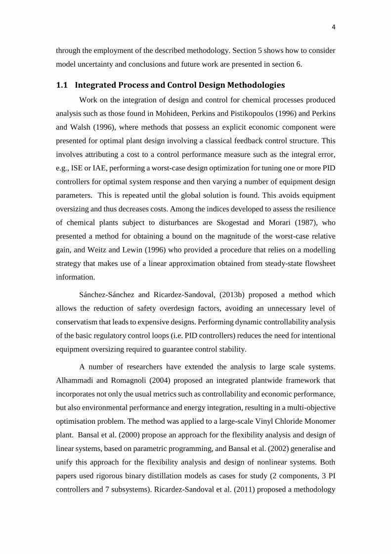
producing off spec products or compromising safety. As can be seen from figure 1, which

presents a simplified scheme to illustrate the economic benefits of MPC, the reduced

variability allows the process to operate closer to restrictions, maximizing output. We

present an approach that explicitly relates the control effort index to plant operational

revenue.

3

Figure 1 – MPC reduces quality give away.

Many years of experience with MPC have shown its ability to improve

performance in this way, but if we can assume this fact how should this affect the

chemical design process? Given a set of controlled and manipulated variables and their

bounds, what effect has a certain plant layout modification on MPC performance? Or how

should changes in product specifications affect the layout if we assume MPC will be

used? The present work proposes an easy new way to assess those impacts that is valid

for any zone constrained MPC algorithm.

The problem being addressed in this work may be summarised as follows: within

the range of all possible operating points or conditions available for a given plant, which

has been defined by the MPC control zones, what is the most profitable? Is the path from

an initial state to this desired state feasible or does it violate soft constraints? Can this

optimal state be sustained by the plant? If we have a number of different plant designs,

how does each plant’s optimal operating point compare? In the current work an optimal

trajectory for each plant is defined, evaluated and inspected by the control engineer who

then proceeds with a comparison between the process candidate designs. The approach

presented in this paper is based on the premise that disturbances are known and estimated

a priori and follow a given time-dependant profile.

This paper is organized in 5 sections. Section 2 contains a brief presentation of the

economic MPC optimization index. Section 3 will feature a case of study concerning the

assessment of four possible layouts for a crude oil distillation unit for which the new

methodology will be applied. Section 4 will present and discuss the results obtained

4

through the employment of the described methodology. Section 5 shows how to consider

model uncertainty and conclusions and future work are presented in section 6.

1.1 Integrated Process and Control Design Methodologies

Work on the integration of design and control for chemical processes produced

analysis such as those found in Mohideen, Perkins and Pistikopoulos (1996) and Perkins

and Walsh (1996), where methods that possess an explicit economic component were

presented for optimal plant design involving a classical feedback control structure. This

involves attributing a cost to a control performance measure such as the integral error,

e.g., ISE or IAE, performing a worst-case design optimization for tuning one or more PID

controllers for optimal system response and then varying a number of equipment design

parameters. This is repeated until the global solution is found. This avoids equipment

oversizing and thus decreases costs. Among the indices developed to assess the resilience

of chemical plants subject to disturbances are Skogestad and Morari (1987), who

presented a method for obtaining a bound on the magnitude of the worst-case relative

gain, and Weitz and Lewin (1996) who provided a procedure that relies on a modelling

strategy that makes use of a linear approximation obtained from steady-state flowsheet

information.

Sánchez-Sánchez and Ricardez-Sandoval, (2013b) proposed a method which

allows the reduction of safety overdesign factors, avoiding an unnecessary level of

conservatism that leads to expensive designs. Performing dynamic controllability analysis

of the basic regulatory control loops (i.e. PID controllers) reduces the need for intentional

equipment oversizing required to guarantee control stability.

A number of researchers have extended the analysis to large scale systems.

Alhammadi and Romagnoli (2004) proposed an integrated plantwide framework that

incorporates not only the usual metrics such as controllability and economic performance,

but also environmental performance and energy integration, resulting in a multi-objective

optimisation problem. The method was applied to a large-scale Vinyl Chloride Monomer

plant. Bansal et al. (2000) propose an approach for the flexibility analysis and design of

linear systems, based on parametric programming, and Bansal et al. (2002) generalise and

unify this approach for the flexibility analysis and design of nonlinear systems. Both

papers used rigorous binary distillation models as cases for study (2 components, 3 PI

controllers and 7 subsystems). Ricardez-Sandoval et al. (2011) proposed a methodology

5

used to estimate analytical bounds on the worst-case variability of disturbances and

parametric model uncertainties suitable for application to large-scale systems (using the

Tenessee Eastman Problem which has 8 components, 8 PI controllers and 5 subsystems).

Trainor et al. (2013) presents a methodology for the optimal process and control design

of large-scale systems under uncertainty that incorporates robust feasibility and stability

analyses formulated as convex mathematical problems (applied to a ternary distillation

problem with 2 PI controllers and 6 subsystems). Alvarado-Morales et al. (2010)

presented an integrated synthesis framework and applied it to two large-scale processes:

a bioethanol production plant as well as succinic acid production (with 16 components, 2

PI controllers and 7 subsystems).

While all systems addressed by works above are genuinely large-scale, oil refining

processes, such as the set of crude oil distillation plants studied here, presents a particular

challenge. The phenomenological models used by the papers presented in this section are

adequate for separation processes of mixtures presenting near-ideal behaviour, i.e., where

deviation from Raoult's law can be ignored, or mixtures of chemically similar solvents,

or non-ideal solutions to which Raoult's law applies and fugacity and activity coefficients

can be easily calculated. But difficulties arise when dealing with petroleum fractions:

each subsystem has usually dozens of non-ideal hypothetical components; severe

operating conditions mean that the behaviour of gases, solutions and mixtures is also non-

ideal; multiphase flow is very common and hard to model adequately; and equipment

designs are intricate. The best simulators for this kind of process do not provide their set

of equations, which are closed source intellectual property. For all these reasons, and the

time and engineering effort required for rigorous modelling is always very large and,

unless models are linearised, even with the optimization solvers and processing power

available at the time of writing it is doubtful that a solution could be found in reasonable

time. This paper aims to offer an alternative controllability analysis approach that is better

suited for the plant-wide design of oil refining processes, and also to include the use of

Model Predictive Control as main control strategy.

1.2 Integrated Process Designs using Model Predictive Control

Adapting this kind of methodology to deal with MPC is a very challenging task

which has been only recently receiving due attention from researchers. Perhaps the first

attempt to extend the classical integrated design and control approach using MPC control

was carried out by Brengel and Seider (1992). Francisco et al. (2011) presented a

6

methodology to provide simultaneously the plant dimensions, the control parameters and

a steady state working point using an IHMPC formulation with a terminal penalty

including considering model uncertainty for robustness. The optimization problem is a

multi-objective nonlinear constrained optimization problem, including capital and

operating costs and controllability indices.

A similar method was presented by Bahakim and Ricardez-Sandoval (2014),

involving the identification of an internal MPC model and solving an optimization

problem at each time step in which the MPC algorithm rejected stochastic worst-case

disturbances. The control performance was added to a design cost function that also

included the capital costs derived from equipment sizing parameters. The methodology

considers how often the worst-case would occur and the level of significance of constraint

violations, arguing that it is not reasonable to overdesign the plant with increased costs

because of extremely rare situations. Chawankul et al. (2007) presented another method

which attributed a variability cost for controlled variables during dynamic operation. The

sum of capital and operating costs are combined into a single objective function. Process

nonlinearity is represented by the use of a nominal linear model with parameter

uncertainty in the MPC internal model. The worst-case variability was quantified and its

associated economic cost was calculated and referred to as the robust variability cost.

This approach avoided nonlinear dynamic simulations, offering computational

advantages.

Sakizlis et al. (2004) presented an extension of the process and control design

framework that incorporates parametric model-based predictive controllers. Applying

parametric programming for the controller derivation, the authors removed the need for

solving an optimization problem on-line by giving rise to a closed-form controller

structure. Sánchez-Sánchez and Ricardez-Sandoval (2013a) solve layers of optimisation

problems: dynamic flexibility analysis, a robust dynamic feasibility analysis, a nominal

stability analysis, and a robust asymptotic stability analysis to determine the optimal

design. The methodology incorporates structural decisions in the analysis for the selection

of an optimal process flowsheet, while formulating the analysis as convex problem for

which efficient numerical algorithms exist. Ricardez-Sandoval et al. (2009) point out that

the algorithmic framework involving MPC is computationally demanding even when a

small number of process units are considered.

7

A different approach to access economic performance is needed to deal with the

multivariable “zone control” problem addressed by most commercial MPC packages.

This variation of a partial control problem is defined by the existence of “zone

constraints” in which every controlled variable is bounded by maximum and minimum

desired values so that the control problem is not to keep each one at a fixed set-point but

instead to keep all of them bounded. Often the MPC is not able to keep all controlled

variables within their control zones due to the lack of degrees of freedom, which may lead

to the violation of some restrictions, which are called ‘soft constraints’. Every

manipulated variable also has its required maximum and minimum values, or ‘hard

constraints’ which must never be violated. It is also a standard feature for industrial

control applications to perform simultaneous process control and optimization. Several

MPC packages, including Honeywell™ MPC, Shell-Yokogawa Exa-SMOC™, Emerson

DeltaV™ Predict and AspenTech DMCplus™ , offer both of these features.

Most recent academic research has been focusing on robust MPC and other

schemes with guaranteed stability, which translate into slower control actions, instead of

real needs and performance (as noted by Bemporad and Morari (1999) robust MPC

control actions may be excessively conservative). Some examples of research concerning

zone control are found in González and Odloak (2009), Grosman et al. (2010), Luo et al.

(2012) and Zhang et al. (2011). Porfírio and Odloak (2011), Gouvêa and Odloak (1998)

and Adetola and Guay (2010) address the integration of economic optimization and MPC

control.

The work presented here aims to provide a workable solution to assess alternative

designs based on control performance and its economic ramifications for highly complex

chemical plants controlled by zone control MPC algorithms. The approach makes use of

the most readily available models, which are usually empirical models identified from

plant tests, such as step tests. Here a new controllability index is used, the economic MPC

optimization index, for assessing process plants for which linear state-space models are

available indicating the best achievable performance by a generic MPC controller. This

index provides results directly related to process economics, taking into account the

required control performance in the face of any given disturbance and process constraints

so as to allow comparison between similar process plants. It will be able to provide a

measure of how much a plant can be optimized while keeping controlled variables within

the bounds of the zone control.

8

2 Some Definitions and Their Use

Let us now define an index to evaluate just how much room for optimization exists

for a given plant when applying a zone constrained model predictive control in the face

of disturbances and control bounds. The goal is to define which candidate plant design

has the best, most profitable and yet reachable state, enabling the analysis and comparison

of slightly different chemical plants in order to find out which one has higher resilience

to disturbances, better controllability, lesser product quality giveaway and lower costs.

Details of the concept of state reachability can be found in Vidyasagar (2002).

In order to be a worthwhile tool for process design the methodology needs to be

carried out independently of other factors such as future choice of MPC algorithm or set

of tuning parameters, focusing only on the model response. Minimizing the index for a

given plant means finding what out what is the best state that can be reached at the end

of the prediction horizon, while subject to zone control. If several chemical plants are

being compared with a view to assessing which has better dynamic response, the optimal

index is closely related to the best achievable performance any MPC package can achieve.

The success of the control effort made by an MPC controller is its capacity to

reject disturbances while optimizing economically the process, and thus the index must

account for the eventual economic losses due to the necessary control actions. The

methodology presented here will favour solutions which have smooth transitions to the

final state and to penalize violations of zone constraints in order to make sure that the

dynamic trajectory leading to the optimized steady-state is feasible. Also, restrictions

concerning manipulated variables such as their maximum rate of change and maximum

and minimum values are incorporated in the analysis.

The index’s purpose is to compare different process plants independently of the

MPC algorithm and tuning parameters that will be used to control these plants.

Considering both the speed of the transient and final values would restrict the validity of

the analysis to a certain algorithm and set of tuning parameters, rendering the analysis

useless otherwise. Furthermore, introducing criteria such as speed of dynamic response

would result in an optimization problem composed of several layers that could be rapidly

become intractable for larger systems, which are the main subjects of this work.

The economic MPC optimization index may be used to determine what are the

best reachable states for a set of chemical plants subject to disturbances and restrictions

9

to inputs and outputs. If these variables, disturbances and restrictions are the same for

those plants, the index indicates the better plant from a dynamic behaviour standpoint:

the lower the index, the better the state reachability for a given plant. Since commercial

MPC packages make use of linear state-space models, which can be identified with

relative ease through step tests of the manipulated inputs, here we use a generic linear

state-space model to obtain the prediction of process outputs y at the end of the prediction

horizon 𝑘 + 𝑝:

𝑦𝑘 = 𝐶𝑥𝑘 (1)

𝑥𝑘+1 = 𝐴𝑥𝑘 + 𝐵∆𝑢𝑘 + 𝐷∆𝑑𝑘 (2)

The model represents a process flowsheet that is assumed to be fixed during the

analysis (this approach does not aim to replace early stage process synthesis usually based

on steady-state information). The method presents analysis of the most promising

flowsheets with regard to zone constrained MPC performance. The goal is to assess which

plant is better placed to accommodate disturbances while being optimized by a MPC.

The model defined by equations (1) and (2) makes use of deviation variables. At

an arbitrary time instant 𝑘, it is possible to predict the values of the process outputs using

the following procedure:

𝑦𝑘+1 = 𝐶𝑥𝑘+1 = 𝐶𝐴𝑥𝑘 + 𝐶𝐵∆𝑢𝑘 + 𝐶𝐷∆𝑑𝑘

𝑦𝑘+2 = 𝐶𝑥𝑘+2 = 𝐶𝐴𝑥𝑘+1 + 𝐶𝐵∆𝑢𝑘+1 + 𝐶𝐷∆𝑑𝑘+1

= 𝐶𝐴2𝑥𝑘 + [𝐶𝐴𝐵 𝐶𝐵] [∆𝑢𝑘∆𝑢𝑘+1

] + [𝐶𝐴𝐷 𝐶𝐷] [∆𝑑𝑘∆𝑑𝑘+1

]

⋮

𝑦𝑘+2 = 𝐶𝐴2𝑥𝑘 + [𝐶𝐴𝐵 𝐶𝐵] [

∆𝑢𝑘∆𝑢𝑘+1

] + [𝐶𝐴𝐷 𝐶𝐷] [∆𝑑𝑘∆𝑑𝑘+1

]

𝑦𝑘+𝑝 = 𝐶𝐴𝑝𝑥𝑘 + [𝐶𝐴

𝑝−1𝐵 𝐶𝐴𝑝−2𝐵… 𝐶𝐴𝑝−𝑚𝐵][∆𝑢𝑘 ∆𝑢𝑘+1… ∆𝑢𝑘+𝑚−1]𝑇 (3)

+[𝐶𝐴𝑝−1𝐷 𝐶𝐴𝑝−2𝐷… 𝐶𝐴2𝐷][∆𝑑𝑘 ∆𝑑𝑘+1… ∆𝑑𝑘+𝑝−3]𝑇

where 𝑚 is the number of time increments of the control horizon, which is also the number

of control actions performed. Here we make the assumption that the number of

disturbance movements is equal to the prediction horizon. This prediction will later be

used to define the economic control resilience index.

10

2.1 Index for Control Bound Violations

In zone control each controlled variable has a minimum and maximum desired

variable but some of these constraints may have more importance than others and, for this

reason, when defining the MPC control problem it is common practice to assign each

controlled variable a weight value, which establishes the relative priority each bound will

have in the solution. For example, constraints relative to process, equipment and

environmental safety normally have precedence over those concerning product

specifications. Henceforth these weight values will be denominated 𝑊𝑖,𝑢𝑝𝑝𝑒𝑟 and 𝑊𝑖,𝑙𝑜𝑤𝑒𝑟

meaning respectively the weights for the upper (maximum value) and lower (minimum

value) bounds of controlled variable 𝑦𝑖, where 𝑖 = 1,… , 𝑛𝑦, and 𝑛𝑦 is the number of

controlled variables. Initially, let us consider the steady-state achieved by the MPC where

the plant will operate for much of the time. The questions of smoothness of the transient

response shall be dealt with in section 2.4, but for now let us just assume that given

enough time the plant will reach steady-state after a series of control and optimization

actions. If only the last instant in the prediction is considered, a new problem arises in

which the goal is to minimize the sum of the predicted deviations from the control zone

for each process output multiplied by its weight. A cost function for this control problem

can be defined as follows:

𝐽𝐶𝑉𝑘+𝑝 = ∑ [|𝑦𝑖,𝑚𝑖𝑛 − 𝑦𝑘+𝑝,𝑖| ∙ 𝑊𝑖,𝑙𝑜𝑤𝑒𝑟 + |𝑦𝑘+𝑝,𝑖−𝑦𝑖,𝑚𝑎𝑥| ∙ 𝑊𝑖,𝑢𝑝𝑝𝑒𝑟]𝑛𝑦𝑖=1 (4)

𝑖𝑓 𝑦𝑖,𝑚𝑖𝑛 ≤ 𝑦𝑘+𝑝,𝑖 ≤ 𝑦𝑖,𝑚𝑎𝑥 ⇒ 𝑊𝑖,𝑢𝑝𝑝𝑒𝑟 = 𝑊𝑖,𝑙𝑜𝑤𝑒𝑟 = 0

𝑖𝑓 𝑦𝑖,𝑚𝑖𝑛 > 𝑦𝑘+𝑝,𝑖 ⇒ 𝑊𝑖,𝑙𝑜𝑤𝑒𝑟 > 0

𝑖𝑓 𝑦𝑘+𝑝,𝑖 > 𝑦𝑖,𝑚𝑎𝑥 ⇒ 𝑊𝑖,𝑢𝑝𝑝𝑒𝑟 > 0

where 𝑖 = 1,… , 𝑛𝑦. In this problem it is of special interest to know if there is a set

of manipulated variables, or MVs, that leads the system to a state where all outputs are

within their zone constraints at the end of the prediction horizon, and thus 𝐽𝐶𝑉𝑘+𝑝 = 0,

or alternatively, if there is no ideal solution for equation 4, what is the final state that

minimizes the violation of the control bounds and consequently minimizes 𝐽𝐶𝑉𝑘+𝑝.

2.2 An Economic Optimization Index

MPC controllers found in the chemical industry frequently possess economic

optimization functions in addition to the control capabilities. Also recent research has

shown that process economics can be optimized directly in the dynamic control problem,

which can take advantage of potentially higher profit transients to give superior economic

11

performance. Examples of this approach include Amrit et al. (2013) and Strutzel et al.

(2013). The optimization is performed by changing the manipulated process inputs when

the process finds itself within its control bounds, and degrees of freedom are available to

be employed in optimization tasks. In oil refining processes, MVs are often related to

process energy cost. For instance, it may be necessary to burn more natural gas in the

fired heater in order to increase the temperature of the feed stream to a reactor. If the feed

temperature is a MV increasing it has a negative impact on process profitability, which

depends on the price of natural gas. Another example would be diesel production in an

atmospheric crude oil distillation column. In this process it is often possible to improve

the quality of the diesel by reducing its output and, consequently, increasing the

atmospheric residue output. However, diesel has a much higher commercial value, so if

the flow rate of diesel is a manipulated variable, it is positively correlated to profitability.

Other MVs are not strongly correlated to energy costs or product prices and can be altered

freely. In inorganic processes the goal is often to maximize chemical reaction conversion

and the relation between MV and costs may be less obvious.

It is thus interesting to define for each MV whether it is positively or negatively

related to profitability, and to what degree. Let us now define two sets of optimization

weights, 𝑉𝑗,𝑚𝑖𝑛 and 𝑉𝑗,𝑚𝑎𝑥, where 𝑗 = 1, … , 𝑛𝑢, where 𝑛𝑢 is the number of MVs, which

illustrate the optimization direction and relative priority among the various MVs for

economic purposes. If a given MV is positively correlated to profitability and at the

present moment is not being employed for control actions, it should stay as close as

possible to its maximum limit or upper bound. Likewise, if it is negatively related to

profitability, it should stay close to its minimum limit or lower bound. In the single layer

MPC control scheme, the optimization weights 𝑉𝑚𝑖𝑛 and 𝑉𝑚𝑎𝑥 are very small compared

to the control zone weights 𝑊𝑖,𝑢𝑝𝑝𝑒𝑟 and 𝑊𝑖,𝑙𝑜𝑤𝑒𝑟 in the cost function, and optimization

is performed without hindering the control objectives. Ferramosca et al. (2014) provide a

formal proof of convergence for such an approach.

Concerning the MVs, it is desired to determine how far they stand from the hard

constraints because, depending on the direction of optimization, this distance denotes how

much room there is for optimization. A simplified optimization cost function may then

be established yielding equation 5, which relates the distance between MVs and their

bounds at the prediction’s end:

12

𝐽𝑀𝑉𝑘+𝑝 = ∑ [|𝑢𝑘+𝑝,𝑗 − 𝑢𝑗,𝑚𝑖𝑛| ∙ 𝑉𝑗,𝑚𝑖𝑛 + |𝑢𝑗,𝑚𝑎𝑥 − 𝑢𝑘+𝑝,𝑗| ∙ 𝑉𝑗,𝑚𝑎𝑥]𝑛𝑢𝑗=1 (5)

Subject to:

𝑢𝑚𝑖𝑛 ≤ 𝑢𝑘+𝑝,𝑗 ≤ 𝑢𝑚𝑎𝑥

where:

𝑢𝑘+𝑝,𝑗 = ∑ ∆𝑢𝑘+𝑗𝑚𝑗=1

The optimization weights are subject to:

𝑉𝑗,𝑚𝑖𝑛 ≥ 0, 𝑉𝑗,𝑚𝑎𝑥 ≥ 0, 𝑉𝑗,𝑚𝑖𝑛 ∙ 𝑉𝑗,𝑚𝑎𝑥 = 0

(6)

where 𝑗 = 1,… , 𝑛𝑢. The set of restrictions defined by equation 6 was included in

order to guarantee that a single economic optimization direction exists for each variable,

if there is any: if for a MV of index 𝑗, 𝑉𝑗,𝑚𝑖𝑛 = 𝑉𝑗,𝑚𝑎𝑥 = 0, then the variable doesn’t have

any optimization direction, being neutral for profitability.

2.3 Economic MPC Optimization Index

Adding equations (4) and (5) in a single cost function yields the first form of the

economic MPC optimization index:

𝐽𝑘+𝑝 = 𝐽𝐶𝑉𝑘+𝑝 + 𝐽𝑀𝑉𝑘+𝑝

= ∑ [|𝑦𝑖,𝑚𝑖𝑛 − 𝑦𝑘+𝑝,𝑖| ∙ 𝑊𝑖,𝑙𝑜𝑤𝑒𝑟 + |𝑦𝑘+𝑝,𝑖−𝑦𝑖,𝑚𝑎𝑥| ∙ 𝑊𝑖,𝑢𝑝𝑝𝑒𝑟]𝑛𝑦𝑖=1

+∑ [|𝑢𝑘+𝑝,𝑗 − 𝑢𝑗,𝑚𝑖𝑛| ∙ 𝑉𝑗,𝑚𝑖𝑛 + |𝑢𝑗,𝑚𝑎𝑥 − 𝑢𝑘+𝑝,𝑗| ∙ 𝑉𝑗,𝑚𝑎𝑥]𝑛𝑢𝑗=1 (7)

Subject to:

𝑖𝑓 𝑦𝑖,𝑚𝑖𝑛 ≤ 𝑦𝑘+𝑝,𝑖 ≤ 𝑦𝑖,𝑚𝑎𝑥 ⇒ 𝑊𝑖,𝑢𝑝𝑝𝑒𝑟 = 𝑊𝑖,𝑙𝑜𝑤𝑒𝑟 = 0

𝑖𝑓 𝑦𝑖,𝑚𝑖𝑛 > 𝑦𝑘+𝑝,𝑖 ⇒ 𝑊𝑖,𝑙𝑜𝑤𝑒𝑟 > 0

𝑖𝑓 𝑦𝑘+𝑝,𝑖 > 𝑦𝑖,𝑚𝑎𝑥 ⇒ 𝑊𝑖,𝑢𝑝𝑝𝑒𝑟 > 0

𝑉𝑗,𝑚𝑖𝑛 ≥ 0, 𝑉𝑗,𝑚𝑎𝑥 ≥ 0, 𝑉𝑗,𝑚𝑖𝑛 ∙ 𝑉𝑗,𝑚𝑎𝑥 = 0

where i = 1,… , ny and j = 1,… , nu. The prediction of 𝑦 at the time instant 𝑘 + 𝑝

is given by equation 3, which can be further simplified by defining the following matrices:

13

𝐶𝑢̿̿ ̿ = [𝐶𝐴𝑝−1𝐵 𝐶𝐴𝑝−2𝐵… 𝐶𝐴𝑝−𝑚𝐵] 𝐶𝑑̿̿ ̿ = [𝐶𝐴

𝑝−1𝐷 𝐶𝐴𝑝−2𝐷… 𝐶𝐴2𝐷]

∆𝑢𝐾 = [∆𝑢𝑘 ∆𝑢𝑘+1… ∆𝑢𝑘+𝑚−1]𝑇 ∆𝑑𝐾 = [∆𝑑𝑘 ∆𝑑𝑘+1… ∆𝑑𝑘+𝑝−3]

𝑇

Replacing these new terms in equation 3 yields:

𝑦𝑘+𝑝 = 𝐶𝐴𝑝𝑥𝑘 + 𝐶𝑢̿̿ ̿ ∆𝑢𝐾 + 𝐶𝑑̿̿ ̿ ∆𝑑𝐾 (8)

The vector 𝑢𝑘+𝑝 may be calculated as follows:

𝑢𝑘+𝑝 = ∑ ∆𝑢𝑘+𝑗 = 𝐼𝑚.𝑛𝑢 ∙ ∆𝑢𝐾𝑚𝑗=1 (9)

where:

𝐼𝑚.𝑛𝑢 = [1 ⋯ 0⋮ ⋱ ⋮0 ⋯ 1

1 ⋯ 0⋮ ⋱ ⋮0 ⋯ 1

⋯ 1 ⋯ 0⋮ ⋱ ⋮0 ⋯ 1

]⏟

}𝑛𝑢

𝑚.𝑛𝑢

(10)

Applying equations 8 and 9 in the cost function 7, and putting the resultant

equation into vector form yields a more functional form for the cost function:

𝐽𝑘+𝑝 = |𝑦𝑚𝑖𝑛 − 𝐶𝐴𝑝𝑥𝑘 − 𝐶𝑢̿̿ ̿ ∆𝑢𝐾 − 𝐶𝑑̿̿ ̿ ∆𝑑𝐾| ∙ 𝑊𝑙𝑜𝑤𝑒𝑟

+|𝐶𝐴𝑝𝑥𝑘 + 𝐶𝑢̿̿ ̿ ∆𝑢𝐾 + 𝐶𝑑̿̿ ̿ ∆𝑑𝐾 − 𝑦𝑚𝑎𝑥| ∙ 𝑊𝑢𝑝𝑝𝑒𝑟 (11)

+|𝐼𝑚.𝑛𝑢 ∙ ∆𝑢𝐾 − 𝑢𝑚𝑖𝑛| ∙ 𝑉𝑚𝑖𝑛 + |𝑢𝑚𝑎𝑥 − 𝐼𝑚.𝑛𝑢 ∙ ∆𝑢𝐾| ∙ 𝑉𝑚𝑎𝑥

For any system described by a state-space model in the form given by equations

1 and 2, subject to a set of disturbance vectors ∆𝑑𝐾 ∈ 𝐷𝐾, the economic MPC

optimization index problem is defined by equation 12. The same restrictions as for

equation 7 apply.

(12)

2.4 Ensuring Viable Solutions

The economic cost function defined in equation 12 guarantees that the final state

will be as close as possible to the economic optimal state without violating the MPC

constraints but does not consider the transient response. Now we shall modify the cost

function to ensure that the transition to the final state is as smooth as possible. In order

to achieve this we now introduce two new parameters in the cost function that will

14

penalize steep changes in the final predicted values for the states, favouring smooth

curves for the controlled variables at the end of the prediction.

These new terms shall be called “soft landing” matrices and will be inversely

proportional respectively to the first and to the second order derivatives of the controlled

variables at instant 𝑘 + 𝑝. By multiplying the economic cost function by the inverses of

the soft landing matrices its value will increase proportionally to the slope of the final

output prediction. The soft landing matrices will be relevant mostly if 𝑝, the prediction

horizon, is small and the system doesn’t have enough time to stabilize. The soft landing

matrices for the first and second order derivatives are:

𝑆𝐿1 = 𝐼𝑛𝑦 − 𝑇𝑆𝐿1[𝑑𝑖𝑎𝑔|𝑦𝑘+𝑝 − 𝑦𝑘+𝑝−1| ∙ 𝑑𝑖𝑎𝑔|𝑦𝑚𝑎𝑥 − 𝑦𝑚𝑖𝑛|−1] (13)

𝑆𝐿2 = 𝐼𝑛𝑦 − 𝑇𝑆𝐿2[𝑑𝑖𝑎𝑔|[𝑦𝑘+𝑝 − 𝑦𝑘+𝑝−1] − [𝑦𝑘+𝑝−1 − 𝑦𝑘+𝑝−2]| 𝑑𝑖𝑎𝑔|𝑦𝑚𝑎𝑥 − 𝑦𝑚𝑖𝑛|−1] (14)

where 𝑇𝑆𝐿1 and 𝑇𝑆𝐿2 are parameter vectors that define the priority of rejecting sharp

moves for each variable. Higher values favour flatter curves at the expense of a more

aggressive approach. Values for 𝑇𝑆𝐿1 and 𝑇𝑆𝐿2 must be assigned so that 1SL and 2SL are

contained in the unit circle. The first order derivative is the difference between the

controlled variable’s predictions at 𝑘 + 𝑝 and 𝑘 + 𝑝 − 1, obtained as follows:

𝑦𝑘+𝑝 − 𝑦𝑘+𝑝−1 = 𝐶𝐴𝑝𝑥𝑘 + [𝐶𝐴

𝑝−1𝐵 𝐶𝐴𝑝−2𝐵… 𝐶𝐴𝑝−𝑚𝐵] [∆𝑢𝑘 ∆𝑢𝑘+1… ∆𝑢𝑘+𝑚−1]𝑇

+[𝐶𝐴𝑝−1𝐷 𝐶𝐴𝑝−2𝐷… 𝐶𝐴2𝐷][∆𝑑𝑘 ∆𝑑𝑘+1… ∆𝑑𝑘+𝑝−3]𝑇

−𝐶𝐴𝑝−1𝑥𝑘 − [𝐶𝐴𝑝−2𝐵 𝐶𝐴𝑝−3𝐵… 𝐶𝐴𝑝−𝑚−1𝐵][∆𝑢𝑘 ∆𝑢𝑘+1… ∆𝑢𝑘+𝑚−1]

𝑇

−[𝐶𝐴𝑝−2𝐷 𝐶𝐴𝑝−3𝐷… 𝐶𝐴𝐷][∆𝑑𝑘 ∆𝑑𝑘+1… ∆𝑑𝑘+𝑝−3]𝑇=

[𝐼𝑛𝑦 − 𝐴−1] = {

𝐶𝐴𝑝𝑥𝑘 + [𝐶𝐴𝑝−1𝐵 𝐶𝐴𝑝−2𝐵… 𝐶𝐴𝑝−𝑚𝐵] [∆𝑢𝑘 ∆𝑢𝑘+1… ∆𝑢𝑘+𝑚−1]

𝑇

+ [𝐶𝐴𝑝−1𝐷 𝐶𝐴𝑝−2𝐷… 𝐶𝐴2𝐷] [∆𝑑𝑘 ∆𝑑𝑘+1… ∆𝑑𝑘+𝑝−3]𝑇 } (15)

Introducing the matrices defined in equation 8, the derivative given by equation

15 becomes:

𝑆𝐿1 = 𝐼𝑛𝑦 −

15

−𝑇𝑆𝐿1[𝑑𝑖𝑎𝑔|[𝐼𝑛𝑦 − 𝐴−1][𝐶𝐴𝑝𝑥𝑘 + 𝐶𝑢̿̿̿̿ ∆𝑢𝐾 + 𝐶𝑑̿̿̿̿ ∆𝑑𝐾]| ∙ 𝑑𝑖𝑎𝑔|𝑦𝑚𝑎𝑥 − 𝑦𝑚𝑖𝑛|

−1] (16)

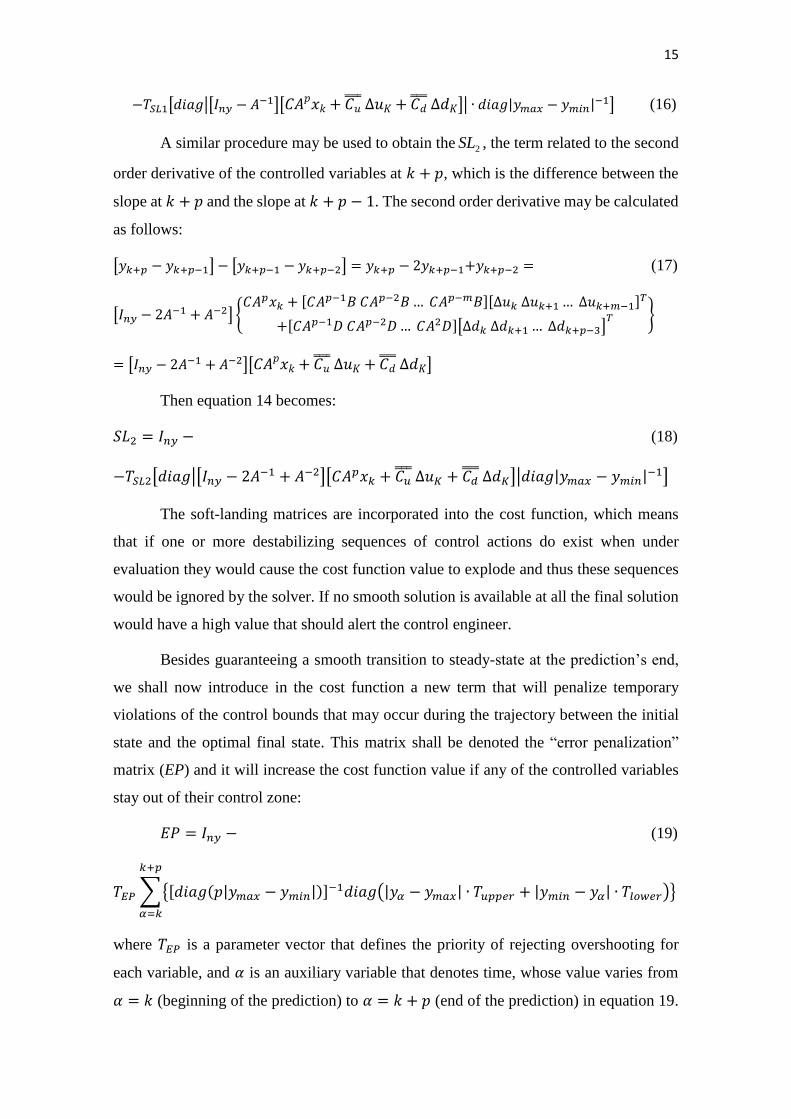
A similar procedure may be used to obtain the 2SL , the term related to the second

order derivative of the controlled variables at 𝑘 + 𝑝, which is the difference between the

slope at 𝑘 + 𝑝 and the slope at 𝑘 + 𝑝 − 1. The second order derivative may be calculated

as follows:

[𝑦𝑘+𝑝 − 𝑦𝑘+𝑝−1] − [𝑦𝑘+𝑝−1 − 𝑦𝑘+𝑝−2] = 𝑦𝑘+𝑝 − 2𝑦𝑘+𝑝−1+𝑦𝑘+𝑝−2 = (17)

[𝐼𝑛𝑦 − 2𝐴−1 + 𝐴−2] {

𝐶𝐴𝑝𝑥𝑘 + [𝐶𝐴𝑝−1𝐵 𝐶𝐴𝑝−2𝐵… 𝐶𝐴𝑝−𝑚𝐵][∆𝑢𝑘 ∆𝑢𝑘+1… ∆𝑢𝑘+𝑚−1]

𝑇

+[𝐶𝐴𝑝−1𝐷 𝐶𝐴𝑝−2𝐷… 𝐶𝐴2𝐷][∆𝑑𝑘 ∆𝑑𝑘+1… ∆𝑑𝑘+𝑝−3]𝑇 }

= [𝐼𝑛𝑦 − 2𝐴−1 + 𝐴−2][𝐶𝐴𝑝𝑥𝑘 + 𝐶𝑢̿̿̿̿ ∆𝑢𝐾 + 𝐶𝑑̿̿̿̿ ∆𝑑𝐾]

Then equation 14 becomes:

𝑆𝐿2 = 𝐼𝑛𝑦 − (18)

−𝑇𝑆𝐿2[𝑑𝑖𝑎𝑔|[𝐼𝑛𝑦 − 2𝐴−1 + 𝐴−2][𝐶𝐴𝑝𝑥𝑘 + 𝐶𝑢̿̿ ̿ ∆𝑢𝐾 + 𝐶𝑑̿̿ ̿ ∆𝑑𝐾]|𝑑𝑖𝑎𝑔|𝑦𝑚𝑎𝑥 − 𝑦𝑚𝑖𝑛|

−1]

The soft-landing matrices are incorporated into the cost function, which means

that if one or more destabilizing sequences of control actions do exist when under

evaluation they would cause the cost function value to explode and thus these sequences

would be ignored by the solver. If no smooth solution is available at all the final solution

would have a high value that should alert the control engineer.

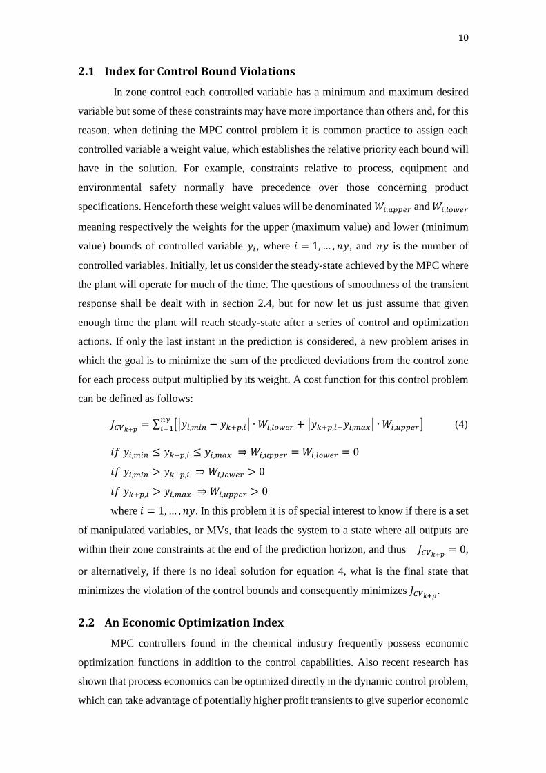
Besides guaranteeing a smooth transition to steady-state at the prediction’s end,

we shall now introduce in the cost function a new term that will penalize temporary

violations of the control bounds that may occur during the trajectory between the initial

state and the optimal final state. This matrix shall be denoted the “error penalization”

matrix (EP) and it will increase the cost function value if any of the controlled variables

stay out of their control zone:

𝐸𝑃 = 𝐼𝑛𝑦 − (19)

𝑇𝐸𝑃∑{[𝑑𝑖𝑎𝑔(𝑝|𝑦𝑚𝑎𝑥 − 𝑦𝑚𝑖𝑛|)]−1𝑑𝑖𝑎𝑔(|𝑦𝛼 − 𝑦𝑚𝑎𝑥| ∙ 𝑇𝑢𝑝𝑝𝑒𝑟 + |𝑦𝑚𝑖𝑛 − 𝑦𝛼| ∙ 𝑇𝑙𝑜𝑤𝑒𝑟)}

𝑘+𝑝

𝛼=𝑘

where 𝑇𝐸𝑃 is a parameter vector that defines the priority of rejecting overshooting for

each variable, and 𝛼 is an auxiliary variable that denotes time, whose value varies from

𝛼 = 𝑘 (beginning of the prediction) to 𝛼 = 𝑘 + 𝑝 (end of the prediction) in equation 19.

16

So 𝑦𝛼 is the vector of controlled variables at time alpha, which is being compared to 𝑦𝑚𝑎𝑥

and 𝑦𝑚𝑖𝑛, in order to know if any controlled variable left the control zone during the

transient. The sets of parameters 𝑇𝑢𝑝𝑝𝑒𝑟 and 𝑇𝑙𝑜𝑤𝑒𝑟 must obey the following restrictions:

𝑖𝑓 𝑦𝑖,𝑚𝑖𝑛 ≤ 𝑦𝑘+𝑝,𝑖 ≤ 𝑦𝑖,𝑚𝑎𝑥 ⇒ 𝑇𝑖,𝑢𝑝𝑝𝑒𝑟 = 𝑇𝑖,𝑙𝑜𝑤𝑒𝑟 = 0

𝑖𝑓 𝑦𝑖,𝑚𝑖𝑛 > 𝑦𝑘+𝑝,𝑖 ⇒ 𝑇𝑖,𝑙𝑜𝑤𝑒𝑟 > 0

𝑖𝑓 𝑦𝑘+𝑝,𝑖 > 𝑦𝑖,𝑚𝑎𝑥 ⇒ 𝑇𝑖,𝑢𝑝𝑝𝑒𝑟 > 0

where 𝑖 = 1,… , 𝑛𝑦. These restrictions guarantee that EP will decrease if, during the

transient, any controlled variable overshoots. If that happens, the solution will be

penalized even if the final state is within its control zone. Matrices 𝑇𝑙𝑜𝑤𝑒𝑟 and 𝑇𝑢𝑝𝑝𝑒𝑟

indicate how strongly this overshooting will be rejected.

Finally, we can reach the final form for the economic MPC optimization index

by multiplying the cost function given by equation 12 by the inverse of the determinants

of the soft landing and the error penalization matrices, 𝑆𝐿1, 𝑆𝐿2 and 𝐸𝑃:

(20)

The new cost function will cause the optimization algorithm to discard

overshooting solutions that could be otherwise selected if equation 12 was used.

Evidently, if 𝑝 is sufficiently large all control actions and their effects will have taken

place at the end of the prediction, 𝑘 + 𝑝, and thus, 𝑆𝐿1 and 𝑆𝐿2 will be identity matrices.

If however, 𝑝 is small or if the set of control actions results in an unstable response, the

index cost function will increase and the solution will be penalized.

The vectors 𝑇𝑆𝐿1, 𝑇𝑆𝐿2, 𝑇𝐸𝑃, 𝑇𝑢𝑝𝑝𝑒𝑟 and 𝑇𝑙𝑜𝑤𝑒𝑟 all require manual tuning. Their

values should reflect prioritization among controlled variables as well the desired balance

between steady-state optimization and penalization for eventual issues in the transient

behaviour. The larger the values, the greater the penalties for lack of a smooth transition

to the final state and for violations of the control zones. The exact values that should be

assigned depend on the number of variables (a larger number of variables increases their

cumulative effect) and the desired penalty. For example, one could tune 𝑇𝐸𝑃, 𝑇𝑢𝑝𝑝𝑒𝑟 and

𝑇𝑙𝑜𝑤𝑒𝑟 in such a way that |𝐸𝑃|−1 = 1 + 1.5 𝑛𝑦⁄ , if a single variable stays unbounded for

50% of the transient, and |𝐸𝑃|−1 = 1 + 1.75 ∙ 1.5 𝑛𝑦⁄ , if additionally another variable is

unbounded for 75% of the transient, and so on. Another possibility is setting 𝑇𝑆𝐿1 and

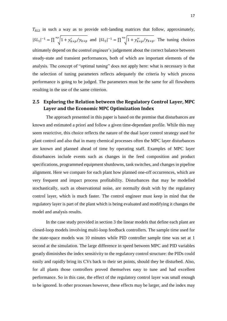
17

𝑇𝑆𝐿2 in such a way as to provide soft-landing matrices that follow, approximately,

|𝑆𝐿1|−1 = ∏ √1+ 𝑦𝑘+𝑝

′ 𝑦𝑘+𝑝⁄𝑛𝑦

and |𝑆𝐿2|−1 = ∏ √1+ 𝑦𝑘+𝑝

′′ 𝑦𝑘+𝑝⁄𝑛𝑦

. The tuning choices

ultimately depend on the control engineer’s judgement about the correct balance between

steady-state and transient performances, both of which are important elements of the

analysis. The concept of “optimal tuning” does not apply here: what is necessary is that

the selection of tuning parameters reflects adequately the criteria by which process

performance is going to be judged. The parameters must be the same for all flowsheets

resulting in the use of the same criterion.

2.5 Exploring the Relation between the Regulatory Control Layer, MPC

Layer and the Economic MPC Optimization Index

The approach presented in this paper is based on the premise that disturbances are

known and estimated a priori and follow a given time-dependant profile. While this may

seem restrictive, this choice reflects the nature of the dual layer control strategy used for

plant control and also that in many chemical processes often the MPC layer disturbances

are known and planned ahead of time by operating staff. Examples of MPC layer

disturbances include events such as changes in the feed composition and product

specifications, programmed equipment shutdowns, tank switches, and changes in pipeline

alignment. Here we compare for each plant how planned one-off occurrences, which are

very frequent and impact process profitability. Disturbances that may be modelled

stochastically, such as observational noise, are normally dealt with by the regulatory

control layer, which is much faster. The control engineer must keep in mind that the

regulatory layer is part of the plant which is being evaluated and modifying it changes the

model and analysis results.

In the case study provided in section 3 the linear models that define each plant are

closed-loop models involving multi-loop feedback controllers. The sample time used for

the state-space models was 10 minutes while PID controller sample time was set at 1

second at the simulation. The large difference in speed between MPC and PID variables

greatly diminishes the index sensitivity to the regulatory control structure: the PIDs could

easily and rapidly bring its CVs back to their set points, should they be disturbed. Also,

for all plants those controllers proved themselves easy to tune and had excellent

performance. So in this case, the effect of the regulatory control layer was small enough

to be ignored. In other processes however, these effects may be larger, and the index may

18

vary considerably according to the selection of control schemes and tuning parameters.

For example, if the regulatory control is too slow or difficult to tune, or if its actuators

run at their saturation limits, then the regulatory layer will have greater impact on the

models and, consequently, on the index.

In the following sections the method is applied to candidate flowsheets for an oil

distillation process unit. For this approach the candidate flowsheets must have their

stability confirmed before applying the economic MPC optimization index. The classical

approach is to use the well-known stability theorem which states that a linearly time

invariant (LTI) system is stable if all eigenvalues of model matrix A have magnitude less

than one, i.e. lie inside the unit circle. According to this definition all flowsheets discussed

in sections 3 and 4 are open loop stable. Details concerning MPC and state-space stability

can be found in Mayne et al. (2000) and Oliveira et al. (1999).

3 Case of Study - Economic Disturbance Index for an Oil

Distillation Process Unit

In order to demonstrate how the economic disturbance cost index may be applied

to provide solutions to industrial scale problems three possible designs for a crude oil

distillation plant shall be presented. Also a common set of controlled and manipulated

variables for the MPC control problem will be defined. As the index is related to the best

possible solution for this control problem, its value will indicate which plant can be better

controlled by a well-tuned MPC controller. In section 7, the index will be evaluated for

each of four different scenarios.

3.1 Describing the Control Problem

The models of the plants presented here were obtained through dynamic

simulation using Honeywell's UniSim® software. They have a very similar design, but

present key differences. These differences represent significant design decisions that the

project engineers have to make through the process of specifying the layout and

dimensions of a chemical plant. The distillation plants are rather simple and have a typical

configuration. The problem has 36 components, 8 local PI controllers, 21 subsystems and

the column has 29 trays. This is considerable larger than the examples reported above.

The base case, or plant 1, can be seen below in figure 2.

19

The process simulated has a realistically drafted layout for a medium sized crude

oil distillation process unit. The distillation column generates 5 different product streams

(Naphtha, Kerosene, Light Diesel, Heavy Diesel and Residue). The Kerosene, Light

Diesel, Heavy Diesel and Residue product streams are used to preheat the crude oil feed

from 25 °C to about 220 °C in two series of heat exchangers, yielding high energetic

efficiency. After the first series the oil reaches an adequate temperature to enter the

desalter drum where salt is removed from the oil. After passing through the second series

of exchangers, the pre-heated oil enters a fired heater where its temperature is increased

to 320-380 °C. The hot crude is then fed to the distillation column where the product

streams are obtained. The cold light diesel and cold heavy diesel streams are mixed

together to generate the “Pool Diesel” stream, whose properties will be used to evaluate

the cost index.

Figure 2 – Plant 1 – Simplified Process Flow Sheet

There are three different types of crude oil available for processing in the three

distillations units: medium (29.0 °API), light (32.3 °API) and heavy (26.2 °API) crude

oils. The light oil provides better yields of the more valuable naphtha, diesel and kerosene

and lower yield of the less desired atmospheric residue. However, it is the most expensive.

The heavy oil provides poor yields of the lighter, more valuable products but on the other

hand it is considerably cheaper. Table 1 provides example costs for the crude oils and the

prices for the products, which will be used in the simulation to calculate the profitability

20

of the process. Those values are based on the average prices for the Brazilian market in

2015, which can be found on ANP (National Agency of Petroleum and Natural Gas)

website.

Medium Crude Oil US$/m3 452.69

Heavy Crude Oil US$/m3 419.17

Light Crude Oil US$/m3 496.76

Naphtha US$/m3 484.84

Kerosene US$/m3 557.83

Diesel US$/m3 551.21

Residue US$/m3 470.17

Table 1 – Crude Oil Costs and Product Prices

The optimization problem for Plant 1, which will be exactly the same for Plants

2, 3 and 4, consists of maximizing the share of Heavy Crude Oil in the feed while

minimizing the share of Light Crude Oil, bringing costs down, and at the same time

increasing the yield of higher priced Diesel and Kerosene in the products. The product

specifications, which act as restrictions for profit maximization, are shown in table 2:

Controlled Variables Description Unit Maximum Minimum

𝒚𝟏 Cetane Index DIESEL - 42

𝒚𝟐 Flash Point DIESEL C - 55

𝒚𝟑 ASTM D86 DIESEL 65% C - 250

𝒚𝟒 ASTM D86 DIESEL 85% C 350 -

𝒚𝟓 ASTM D86 DIESEL 95% C 370 -

𝒚𝟔 Freezing Point DIESEL C -15 -

𝒚𝟕 Density (15 C) DIESEL kg/m3 860 820

𝒚𝟖 ASTM D86 KEROSENE 100% C 300 -

𝒚𝟗 Flash Point KEROSENE C - 38

𝒚𝟏𝟎 Density (15 C) KEROSENE kg/m3 840 775

𝒚𝟏𝟏 Freezing Point KEROSENE C -47 -

Table 2 – Description and limits for the controlled variables.

It is also interesting to control Kerosene’s properties. Table 2 below provides a

list of the controlled variables whose limits must be enforced by an MPC controller and

must be taken into account while evaluating the economic disturbance cost index. The

values below are true specifications for the fuels marketed in the European Union.

The manipulated variables available to the MPC controller and their limits can be

found in table 3. The plant has a number of PID feedback controllers and the plant state-

space model is a closed loop model. In a classic two layer control framework, the MPC

manipulated variables are the PID controllers’ set points.

21

Manipulated Variables Description Unit Maximum Minimum

𝒖𝟏 Temperature 01 tray TIC01.SP C 70 40

𝒖𝟐 Temperature Fired Heater TIC02(B).SP C 380 320

𝒖𝟑 Light Diesel Output FC02.SP m3/h 270 (*) 0

𝒖𝟒 Heavy Diesel Output FC03.SP m3/h 65 (*) 0

𝒖𝟓 Medium Crude Flow Rate FC01A.SP m3/h 800 (**) 0

𝒖𝟔 Light Crude Flow Rate FC01B.SP m3/h 800 (**) 0

𝒖𝟕 Heavy Crude Flow Rate FC01C.SP m3/h 800 (**) 0

Table 3 – Description and limits for the manipulated variables. *Total diesel

production (sum of 𝑢3 and 𝑢4) must be at least 85 m3/h. **The sum of 𝑢5, 𝑢6 and

𝑢7 must be equal to 800 m3/h, keeping the total feed flow constant.

A slop recycle will be used as a measured disturbance. Processes such as

atmospheric or vacuum distillation produce several main cuts as well as slop cuts. Slop

oil is the collective term for mixtures of heavy fractions of oil, chemicals and water

derived from a wide variety of sources in refineries or oil fields, often forming emulsions.

For example, in a vacuum distillation unit the slop oil and water are separated by gravity

in the vacuum drum. It is also formed when tank wagons and oil tanks are cleaned and

during maintenance work or in unforeseen oil accidents. Slop oil formation can be

reduced but cannot be avoided and the need to dispose of it results in one of the largest

challenges in the everyday operation of an oil refinery.

The slop cuts produced during the operation of oil refining are conventionally

stored in large oil lagoons or tanks to receive chemical treatment so as to enable them to

be recycled to process units such as fluid catalytic cracking or, very often, atmospheric

distillation units. Therefore, slop oil must be incorporated into the process feed from time

to time. In the distillation unit simulated in this work, it is possible to treat the recycle of

slop oil as a disturbance and measure the impact of changes in its flow rate in the

controlled variables. The same set of variables was defined for all three plants, and a state

space model for every pair of input and output has been identified through step tests

carried out by dynamic simulation. These models are shown in the appendix.

Plant 2 is essentially the same process as plant 1, with the exception of the

presence of two product tanks which collect respectively the kerosene and pool diesel

output streams. The kerosene tank is 616 m3 and the diesel tank is 1692 m3, which implies

a residence time of 10 hours for both the kerosene and diesel streams if flow rates remain

at their steady state values. In plant 2, instead of being concerned about the properties of

distillation column side streams of diesel and kerosene as in plant 1, it is desired to control

22

the properties of the diesel and kerosene streams exiting the product tanks. Plant 2 is

presented in figure 4. The virtual analysers AI01 and AI02 are placed in different

positions compared to figure 3, i.e., after the diesel and kerosene product tanks instead of

after the column.

Figure 3 – Plant 2 – Simplified Process Flow Sheet – Plant with Product Tanks.

Plant 3 and 4 are also very similar to plant 1, but with distillations columns of

remarkably different dimensions. Plant 3’s column is of increased size compared to plants

1 and 2’s, while Plant 4’s has a smaller column accompanied of a pre-flash drum that

removes the lighter fractions such as C1-C4 gases and light naphtha and an extra fired

heater. This new fired heater ensures the feed has an appropriate relation between gas and

liquid phases. Plant 3’s column may be considered to be slightly oversized for the

nominal feed flow rate of 800 m3/h, and the interesting point here is the slower dynamic

response provided by a larger column. Plant 4’s pre-flash drum has a volume of 12.56 m3.

In section 5 it shall be discussed how these differences may affect the process

controllability by a MPC controller. The differences in the sizing parameters of the

columns in plant 1, 2, 3 and 4 (column height and number of trays are the same) are shown

in table 4:

Plant 1 and 2 Plant 3 Plant 4

Column Diameter (m) 13.7 15 11.62

Tray Space (m) 0.60 0.70 0.51

Tray Volume (m3) 88.45 123.7 52.1

23

Weir Height (mm) 50 65 42.40

Weir Length (m) 10.0 14.0 7.9

Downcomer Volume (m3) 0.08836 0.1 0.08836

Internal Type Sieve Bubble Cap Sieve

Table 4 – Column Sizing Parameters for Plants 1, 2, 3 and 4.

Figure 4 – Plant 4 – Simplified Process Flow Sheet – Plant with Pre-flash Drum.

3.2 State-Space Model Formulation

The state-space formulation for this plant is presented in Strutzel et al. (2013) and

is built upon the transfer functions that can be obtained from the analytical form of the

step response of the system, a convenient and common way of obtaining the models of a

chemical plant. Therefore, this formulation was selected for use in the case study

discussed in this section. More details and further developments about this kind of model

representation, designated output prediction oriented model (OPOM), which was first

proposed by Rodrigues and Odloak (2000), can be found in Martins et al. (2013) and

González et al. (2007).

3.3 Measuring the Economic Impact of the Control Effort

In the case of an oil distillation unit, it is necessary to burn more natural gas in the

fired heater in order to increase the temperature of the feed stream to the column.

Therefore, since the feed temperature is a manipulated variable increasing it has a

negative impact on process profitability, which depends on the price of natural gas. Thus,

2u is negatively correlated to profitability.

24

The MPC controller also should be able to maintain the diesel output at the

maximum value that guarantees a specified product, without reducing output

unnecessarily. The commercial value of the residue stream is much lower than that of the

diesel, thus transferring hydrocarbons from the diesel to residue decreases revenue.

Therefore, 𝑢4 is positively correlated to profitability.

Finally, the composition of the feed is also defined by the MPC controller. It is

able to manipulate the flow rate of Light, Medium and Heavy oil crudes in order to keep

specifications within constraints, decreasing the volume of heavy oil and increasing light

oil when necessary. Once more, there is a trade-off between profitability and product

specifications, because lighter crudes usually generate better products but also cost more.

The medium crude will make the bulk of the feed and has properties in between those of

heavy and light oil.

3.4 Defining Parameters for measuring Economic Control Cost

As discussed in section 2, each of the process inputs and outputs requires a

weighting parameter to which the analysis is highly sensitive. In this section adequate

values for these shall be defined using market prices for the crude oil feed, product

streams, energy costs and data from the simulation.

𝑢1 – Temperature 01 tray (TIC01.SP)

Concerning the distillation column top temperature control, there is an energetic

cost to decreasing it due to the fact that more cooling water will be spent in order to

increase the reflux flow rate. Calculating the cost of generating cooling water is a complex

task, but it can all nevertheless be assumed that this cost is insignificant compared the

other costs involved and therefore will be considered equal to zero. Thus, it is assumed

that 𝑉1,𝑚𝑖𝑛 = 𝑉1,𝑚𝑎𝑥 = 0.

𝑢2 – Temperature Fired Heater (TIC02.SP / TIC02B.SP)

It is possible to establish a relation between the crude oil temperature at the fired

heater outlet and the heat duty for plant 1,2 and 3. At a fixed feed flow of 800 m3/h, the

simulation provides the values found in table 5 below:

T (C) Q (Mcal/h)

330.07 61,066

334.11 62,406

335.13 62,676

336.10 62,966

25

340.00 64,332

Table 5 – Energy consumption by the fired heater

where T is the fired heater outlet temperature and Q is the heat duty. From the values

above we obtain the increase in energy consumption relative to the increase in outlet

temperature, as shown in table 6:

ΔT

(C)

ΔQ

(Mcal/h)

ΔQ/ΔT

(Mcal/(C.h))

4.04 1,339.8 331.4

1.02 270.8 265.5

0.97 289.8 299.2

3.90 1,365.5 349.9

Table 6 – Increase in energy consumption by the fired heater

Clearly, the energy cost is dependent on the starting temperature and the

relationship is nonlinear. It also depends on the feed flow to the column. However, for

control purposes the values are close enough and an average value can be used without

any compromises to control performance. The average of ΔQ/ΔT = 311.5 Mcal/(C.h)

shall be considered at any feed flow rate. Considering the Lower Heating Value (LHV)

of natural gas equal to 8.747 Mcal/m3 and a natural gas price of 0.33 US$/m3, the cost

related to 𝑢2 can be calculated as follows:

𝑉2,𝑚𝑖𝑛 =∆𝑄 ∆𝑇⁄

𝐿𝐻𝑉 𝑃𝑁𝐺 =

311.5 𝑀𝑐𝑎𝑙 𝐶. ℎ⁄

8.747 𝑀𝑐𝑎𝑙 𝑚3⁄ 0.33

𝑈𝑆$

𝑚3= 11.75

𝑈𝑆$

𝐶. ℎ

𝑉2,𝑚𝑎𝑥 = 0

For plant 4 𝑢2 is defined as the temperature at the fired heater B outlet. Because

the light components are separated from the feed at the pre-flash drum, the feed properties

and, thus the heat exchange coefficients, are slightly different. However, for the sake of

simplicity this difference will be ignored since its effects are very small.

𝑢3/𝑢4 – Light Diesel Output (FC02.SP) and Heavy Diesel Output (FC03.SP)

In this example the light and heavy diesel streams are combined to produce the

“pool diesel”. The kerosene output and diesel output are placed sequentially in the boiling

point curve and therefore transferring hydrocarbons between these streams is part of

normal of everyday operations. However, the UNISIM simulation used in this example

considers a fixed kerosene output in order for the simulator to be able to solve the fluid

flow dynamic equations. However there is a variable flux between the diesel output and

26

the residue output and thus the optimization gain is defined as the price difference

between these streams:

𝑉3,𝑚𝑎𝑥 = 𝑉4,𝑚𝑎𝑥 = 𝑃𝑑𝑖𝑒𝑠𝑒𝑙 − 𝑃𝑟𝑒𝑠𝑖𝑑𝑢𝑒 = 551.21 − 470.17 = 81.04𝑈𝑆$

𝑚3

𝑉3,𝑚𝑖𝑛 = 𝑉4,𝑚𝑖𝑛 = 0

As discussed at the beginning of this section, increasing heavy diesel output

reduces the residue output and thus increases profitability. In this case study the

separation between light and heavy diesel output has no commercial importance but in

most refineries these hydrocarbon streams have different destinations, such as being fed

to different hydrotreating or hydrocracking process units, and therefore they may have

different commercial values. These possibilities are not considered here.

5u – Medium Crude Oil Feed Flow Rate (FC01A.SP)

Given a set of flow rate values for each of the crude oils that compose the feed to

the distillation column, at any given time the average price of the oil processed is given

by:

𝑃𝑎𝑣𝑒 =452.69 𝑢5 + 496.76 𝑢6 + 419.17 𝑢7

𝑢5 + 𝑢6 + 𝑢7 𝑈𝑆$

𝑚3

The difference between average oil price and the medium crude will provide the

optimization coefficient.

∆𝑃𝑚𝑒𝑑𝑖𝑢𝑚 = 𝑃𝑚𝑒𝑑𝑖𝑢𝑚 − 𝑃𝑎𝑣𝑒

Therefore the following rule may be defined to obtain 𝑉5,𝑚𝑖𝑛 and 𝑉5,𝑚𝑎𝑥:

𝑖𝑓 ∆𝑃𝑚𝑒𝑑𝑖𝑢𝑚 > 0 ⟹ 𝑉5,𝑚𝑎𝑥 = 0, 𝑉5,𝑚𝑖𝑛 = ∆𝑃𝑚𝑒𝑑𝑖𝑢𝑚

𝑖𝑓 ∆𝑃𝑚𝑒𝑑𝑖𝑢𝑚 < 0 ⟹ 𝑉5,𝑚𝑎𝑥 = −∆𝑃𝑚𝑒𝑑𝑖𝑢𝑚, 𝑉5,𝑚𝑖𝑛 = 0

𝑖𝑓 ∆𝑃𝑚𝑒𝑑𝑖𝑢𝑚 = 0 ⟹ 𝑉5,𝑚𝑎𝑥 = 𝑉5,𝑚𝑖𝑛 = 0

In the third case, all feed is already entirely composed of medium crude and

average oil price doesn’t change with changes in 𝑢5.

𝑢6– Light Crude Oil Feed Flow Rate (FC01B.SP)

In a similar manner to the approach used for 𝑢5, the difference between average

oil price and the medium crude will provide the optimization coefficient 𝑉6,𝑚𝑖𝑛, and since

the light oil is the most expensive, the maximization coefficient will always be zero.

27

𝑉6,𝑚𝑖𝑛 = ∆𝑃𝑙𝑖𝑔ℎ𝑡 = 𝑃𝑙𝑖𝑔ℎ𝑡 − 𝑃𝑎𝑣𝑒 𝑉6,𝑚𝑎𝑥 = 0

𝑢7 – Heavy Crude Oil Feed Flow Rate (FC01C.SP)

In a similar manner to the approach used for 5u and 6u , the difference between an

average oil price and the medium crude will provide the optimization coefficient 𝑉7,𝑚𝑎𝑥,

and since the light oil is the most expensive, the minimization coefficient will always be

zero:

𝑉7,𝑚𝑎𝑥 = ∆𝑃ℎ𝑒𝑎𝑣𝑦 = 𝑃𝑎𝑣𝑒−𝑃ℎ𝑒𝑎𝑣𝑦 𝑉7,𝑚𝑖𝑛 = 0

𝑑 – Disturbance slop recycle

While in operating refineries slop streams require an expensive previous treatment

in order to be incorporated into the feed and reprocessed, in this study this element of

process economics will be ignored. It will not change the analysis since the MPC is not

able to determine slop flow rate in first place. Being a disturbance, the slop will not have

a price tag in the optimization problem, and thus may be considered a feed component

whose hydrocarbons are available for “free” for they do not need to be acquired and, once

these slop hydrocarbons replace crude oil in the feed and are recovered and incorporated

in the product cuts, they cause the overall index to decrease. At the same time, since slop

is composed mostly of very heavy, difficult to process oil cuts it diminishes the maximum

quantity of cheap heavy oil that can be processed and increases the energy consumption,

and in its turn these effects increase the index. The absolute values are not consequential:

the goal is to evaluate the relative performance of each plant which is going to behave

differently due to the presence of slop in the feed.

Controlled Variables

To avoid having controlled variables out of their control zones due to the

optimization efforts, the parameters 𝑊𝑢𝑝𝑝𝑒𝑟 and 𝑊𝑙𝑜𝑤𝑒𝑟 must have high enough values

that the cost generated by one or more process outputs outside their control zone is much

higher than the cost due to optimization. From an economic perspective, since product

specifications are requirements for the product to be saleable, the optimization weight for

each controlled value can be defined as the value of the relevant product stream as

provided in Table 1. Since 𝑦1 to 𝑦7 are related to diesel specifications, the cost of violating

their restrictions will be equal to the diesel price multiplied by diesel output, which is

defined as the sum of 𝑢3 and 𝑢4. In this case study the possibility of selling diesel and

28

kerosene as fuel oil is not being considered, and such a procedure is also very unlikely in

industrial operations.

551.21𝑈𝑆$

𝑚3(𝑢3 + 𝑢4)

𝑚3

(10 𝑚𝑖𝑛)= 551.21(𝑢3 + 𝑢4)

𝑈𝑆$

(10 𝑚𝑖𝑛)

Similarly, 𝑦8 to 𝑦11 are related to kerosene specifications, and their weight in the

optimization problem will be equal to the kerosene price multiplied by kerosene output,

which is kept fixed at 61.29 m3/h, or 10.215 m3/(10 min).

557.83𝑈𝑆$

𝑚310.215

𝑚3

(10 𝑚𝑖𝑛)= 5698.23

𝑈𝑆$

(10 𝑚𝑖𝑛)

Hence, the set of rules below was adopted for defining the weights of each

controlled variable in the cost function:

𝑖𝑓 𝑦𝑖,𝑚𝑖𝑛 ≤ 𝑦𝑘+𝑝,𝑖 ≤ 𝑦𝑖,𝑚𝑎𝑥 ⟹ 𝑊𝑖,𝑙𝑜𝑤𝑒𝑟 = 𝑊𝑖,𝑢𝑝𝑝𝑒𝑟 = 0

𝑖𝑓 𝑦𝑖,𝑚𝑖𝑛 > 𝑦𝑘+𝑝,𝑖 ⟹ 𝑊𝑖,𝑙𝑜𝑤𝑒𝑟 = 551.21(𝑢3 + 𝑢4), 𝑖 = 1,2,3,4,5,6,7

𝑖𝑓 𝑦𝑘+𝑝,𝑖 > 𝑦𝑖,𝑚𝑎𝑥 ⟹ 𝑊𝑖,𝑢𝑝𝑝𝑒𝑟 = 551.21(𝑢3 + 𝑢4), 𝑖 = 1,2,3,4,5,6,7

𝑖𝑓 𝑦𝑖,𝑚𝑖𝑛 > 𝑦𝑘+𝑝,𝑖 ⟹ 𝑊𝑖,𝑙𝑜𝑤𝑒𝑟 = 5698.23, 𝑖 = 8,9,10,11

𝑖𝑓 𝑦𝑘+𝑝,𝑖 > 𝑦𝑖,𝑚𝑎𝑥 ⟹ 𝑊𝑖,𝑢𝑝𝑝𝑒𝑟 = 5698.23, 𝑖 = 8,9,10,11

4 Results and Discussion

In this section the results obtained through the application of the economic MPC

optimization index to assessing alternative distillation plant designs are presented. The

optimization problem was solved using the interior-point routine available in the

optimization toolbox in Matlab. It is also worth noting that the problem has nonlinear

constraints and required a solver able to deal with disjunctive programming. However, in

some cases the results proved to be sensitive to the initial point chosen, and the

optimization algorithm sometimes reached a local minimum instead of a global one. To

avoid this shortcoming an iterative “genetic” algorithm strategy was implemented

consisting of using the previous solution the new starting point, but randomly modifying

it so as to implement “mutations”, then evaluating the cost function and storing the new

solution if it was better than the previous one. The random mutations were constrained to

be within ±25% of the acceptable range for each manipulated variable and 100 iterations

were permitted using this methodology in each case. While we believe the solutions

presented are global, no formal proof will be provided.

29

4.1 Scenario 1 – Simultaneous Control and Optimization without

Disturbance

The four different plants were given the same starting point, i.e. the same initial

values for the controlled and manipulated variables. Given this set of values, it is

necessary to obtain the initial state vector, 𝑥𝑘 for each plant. For the state-space model

employed, a completely null state vector (𝑥𝑘 = 0) is the model’s origin, or the equivalent

of having the plant at the exact same steady state used during the step test model

identification. To test a different starting points equation 21 gives initial states:

𝑦𝑘 = 𝐶𝑥𝑘 ⟹ 𝑥𝑘 = 𝐶−1𝑦𝑘 (21)

but there are an infinite number of potential solutions to equation 21 and future states may

also be affected the choice of 𝑥𝑘, as can be seen by equation 3. To make sure a “coeteris

paribus” comparison is possible, it is convenient to implement equation 21 as a restriction

that ensures the selection of a stable state, which satisfies equation 21 while having no

impact on future states 𝑥𝑘+1, 𝑥𝑘+2, … , 𝑥𝑘+𝑝. The restriction defined by equation 22

satisfies these criteria:

0 = ∑ |yk − CAzxk|

pz=0 (22)

For all the plants studied it was possible to obtain kx that satisfied equations 21

and 22. The same values for the controlled and manipulated variables resulted in distinct

vectors 𝑥𝑘 since each plant has its own model. Although we recommend several distinct

starting points to be tested for thorough analysis, due to lack of space our analysis will be

carried out using the single one given in table 7:

𝐲𝟏 𝒚𝟐 𝒚𝟑 𝒚𝟒 𝐲𝟓 𝐲𝟔 𝒚𝟕 𝒚𝟖 𝒚𝟗 𝐲𝟏𝟎 𝐲𝟏𝟏

System

origin 44.00 81.76 288.82 319.42 341.42 -25.47 826.79 251.11 49.79 812.88 -68.38

Starting

point 43.28 83.95 292.39 318.69 341.70 -25.60 829.33 251.48 50.82 815.75 -68.62

Table 7 – New initial values for process outputs.

The assigned value for controlled variable 𝑦1, the Cetane Index, is set lower than

its required value of 46. This requires control actions to bring 𝑦1 back to its control zone

and this control effort may limit the room for optimization. In this first scenario, which

may serve as a basis of comparison with other cases, the processes are at steady-state and

there is no disturbance. Optimization was carried out with the restriction of constant total

feed flow and the set of parameters introduced in section 4 for plants 1, 2, 3 and 4, and

30

using a control horizon 𝑚 = 6, a prediction horizon 𝑝 = 60 (10 hours) and 𝑇𝑆𝐿1 and 𝑇𝑆𝐿2

equal to unitary vectors multiplied by scalar 5. The weights 𝑇𝑙𝑜𝑤𝑒𝑟 and 𝑇𝑢𝑝𝑝𝑒𝑟 are unitary

vectors when variables are outside their control zones and null when they are within. The

MVs in table 8 (only final values are shown) were found to be the best available for each

plant:

Manipulated Variables

Description

Unit Max.

Value

Min.

Value

Initial

Value

Final Value

Plant

1

Plant

2

Plant

3

Plant

4

𝒖𝟏 Temperature 01 tray TIC01.SP C 70.0 40.0 42.64 40.00 41.27 69.63 40.01

𝒖𝟐 Temperature Fired Heater TIC02.SP C 380.0 320.0 335.13 379.99 320.00 380.00 346.06

𝒖𝟑 Light Diesel Output FC02.SP m3/h 270.0(*) 0.0 135.75 62.00 145.03 58.69 61.22

𝒖𝟒 Heavy Diesel Output FC03.SP m3/h 65.0(*) 0.0 25.71 49.37 0.00 26.53 64.99

𝒖𝟓 Medium Crude Flow Rate FC01A.SP m3/h 800 (**) 0.0 550.00 112.09 288.70 1.36 753.47

𝒖𝟔 Light Crude Flow Rate FC01B.SP m3/h 800 (**) 0.0 250.00 0.11 511.29 11.17 0.07

𝒖𝟕 Heavy Crude Flow Rate FC01C.SP m3/h 800 (**) 0.0 0.00 687.81 0.01 787.46 46.47

𝒅𝟏 Slop Oil Feed Recycling Flow Rate m3/h 0.00 0.00 0.00 0.00 0.00 0.00 0.00

Table 8 – Inputs for case without disturbance. *u3 + u4 ≥ 85 **u5 + u6 + u7 = 800.

For these sets of process inputs, the cost function values for each plant are

provided in table 9. Lower values are better and thus plant 3 presented the best

performance, closely followed by plant 1, while plants 2 and 4 had worse results. The

lower values of the index result from larger amount of cheaper heavy crude oil that could

be processed in plant 3 and 1. Comparing plants 2 and 4, the latter performed better since

it did not require a large proportion of light oil in order to avoid producing off-spec

products.

Plant 1 Plant 2 Plant 3 Plant 4

Objective

Function Value 5639.5 12693.0 5516.2 8920.14

Table 9 – Cost Function Values for each Plant – Case 1.

Table 10 provides values for the controlled outputs for each plant. In all three

cases the algorithm was able to define a set of inputs that guarantee that no output value

violated its zone bounds during the transient or at their final values. The highlighted

values show which boundary conditions were active for each plant, which were the

quality requirements that restricted profitability.

31

Controlled Variables Description Unit Min.

Value

Max.

Value

Initial

Value

Final Value

Plant

1

Plant

2

Plant

3

Plant

4

𝒚𝟏 Cetane Index DIESEL 46.0 - 44.00 46.00 46.00 46.00 46.00

𝒚𝟐 Flash Point DIESEL C 55.0 - 81.76 145.66 89.31 86.48 95.57

𝒚𝟑 ASTM D86 DIESEL 65% C 250.0 - 288.81 309.46 301.96 307.47 305.82

𝒚𝟒 ASTM D86 DIESEL 85% C - 350.0 319.42 334.71 346.00 322.23 348.18

𝒚𝟓 ASTM D86 DIESEL 95% C - 370.0 341.63 355.07 369.94 339.75 355.70

𝒚𝟔 Freezing Point DIESEL C - -15.0 -25.47 -15.00 -18.75 -15.00 -15.00

𝒚𝟕 Density (15 C) DIESEL kg/m3 820.0 860.0 826.79 860.00 822.51 859.93 859.11

𝒚𝟖 ASTM D86 KEROSENE 100% C - 300.0 251.11 242.67 253.33 243.74 292.88

𝒚𝟗 Flash Point KEROSENE C 38.0 - 49.79 123.76 58.09 129.20 95.41

𝒚𝟏𝟎 Density (15 C) KEROSENE kg/m3 775.0 840.0 812.88 813.65 816.11 808.40 822.84

𝒚𝟏𝟏 Freezing Point KEROSENE C - -47.0 -68.38 -67.26 -64.10 -68.95 -70.63

Table 10 – Output predictions for scenario without disturbance.

4.2 Scenario 2 – Handling a Measured Disturbance

In this scenario the process simulations start at the same steady-state and all

parameters were kept at the same values as in case 1. However, the slop recycling flow

rate, which acts as a measured disturbance, was increased from zero to 90 m3/h at time

instant 𝑘, and kept at this value and until 𝑘 + 𝑝. The total crude oil flow rate, composed

of light, medium and heavy crudes, was decreased from 800 m3/h to 710 m3/h in order to

accommodate the flow of slop, while keeping total volumetric flow constant. As in case

1, the minimum limit for the Cetane Index, controlled variable 𝑦1, is 46 and the initial

value is lower than required. Table 11 presents the inputs for each plant:

Manipulated Variables

Description Unit

Max.

Value

Min.

Value

Initial

Value

Final Value

Plant

1

Plant

2

Plant

3

Plant

4

𝒖𝟏 Temperature 01 tray TIC01.SP C 70.0 40.0 42.64 40.00 40.00 69.99 40.00

𝒖𝟐 Temperature Fired Heater TIC02.SP C 380.0 320.0 335.13 379.98 320.00 380.00 332.93

𝒖𝟑 Light Diesel Output FC02.SP m3/h 270.0(*) 0.0 135.75 68.31 154.92 69.10 140.21

𝒖𝟒 Heavy Diesel Output FC03.SP m3/h 65.0(*) 0.0 25.71 46.70 0.03 26.56 65.00

𝒖𝟓 Medium Crude Flow Rate FC01A.SP m3/h 800 (**) 0.0 550.00 0.01 23.59 92.24 603.23

𝒖𝟔 Light Crude Flow Rate FC01B.SP m3/h 800 (**) 0.0 250.00 146.46 686.41 94.96 0.03

𝒖𝟕 Heavy Crude Flow Rate FC01C.SP m3/h 800 (**) 0.0 0.00 563.53 0.00 522.81 196.73

𝒅𝟏 Slop Oil Feed Recycling Flow Rate m3/h 0.00 0.00 0.00 90.00 90.00 90.00 90.00

Table 11 – Inputs for specification change case. *u3 + u4 ≥ 85 **u5 + u6 + u7 = 800.

The index values for this scenario can be found in table 12. This time plant 4 had

the best performance and plant 1 and 3 followed quite closely. Plant 2 had the worst result

yet again, with significantly higher index due to its slower dynamics which prevented it

from producing properly specified diesel (see table 13). Compared to plants 1 and 3, plant

4 could produce more diesel and for this reason had a better index.

32

Plant 1 Plant 2 Plant 3 Plant 4

Objective

Function Value 7576.9 34718.4 7690.1 6987.23

Table 12 – Cost Function Values for each Plant – Case 2.

Direct comparison of index values between cases 1 and 2 should take into account

that case 2 involves lower crude oil flow rates. Compared to case 1, the index was 34.35%

higher for plant 1. Plant 2 had an index 173.52% higher; plant 3, 39.41% higher and plant

4, a 21.66% lower index. Therefore, the performance degradation due to the disturbance

was relatively small for plants 1 and 3, and very significant for plant 2. The fact that those

plants had lower indices confirms the expected decrease in profitability due to the need

to meet quality requirements in the presence of slop in the oil feed, leading to higher crude

oil acquisition costs (increased demand for expensive light and medium oils). However,

plant 4 made good use of the “free” raw material provided by the slop, and its performance

actually improved. Concerning the outputs, we can observe in table 13 that the final

cetane value, 𝑦1, for plant 2 was not met even with almost all the feed composed of light

oil. This signifies that plant layout 2 cannot handle a slop recycle of 90 m3/h without

compromising product quality.

Controlled Variables Description Unit Min.

Value

Max.

Value

Initial

Value

Final Value

Plant

1

Plant

2

Plant

3

Plant

4

𝒚𝟏 Cetane Index DIESEL 46.0 - 44.00 46.02 45.78 46.39 46.00

𝒚𝟐 Flash Point DIESEL C 55.0 - 81.76 115.16 85.75 89.13 89.24

𝒚𝟑 ASTM D86 DIESEL 65% C 250.0 - 288.81 309.91 280.16 308.18 330.93

𝒚𝟒 ASTM D86 DIESEL 85% C - 350.0 319.42 335.51 345.97 324.00 350.00

𝒚𝟓 ASTM D86 DIESEL 95% C - 370.0 341.63 359.02 370.00 345.48 339.34

𝒚𝟔 Freezing Point DIESEL C - -15.0 -25.47 -15.00 -15.00 -15.00 -15.16

𝒚𝟕 Density (15 C) DIESEL kg/m3 820.0 860.0 826.79 859.56 821.35 858.32 840.17

𝒚𝟖 ASTM D86 KEROSENE 100% C - 300.0 251.11 245.71 253.36 252.58 251.60

𝒚𝟗 Flash Point KEROSENE C 38.0 - 49.79 117.02 59.29 110.37 68.56

𝒚𝟏𝟎 Density (15 C) KEROSENE kg/m3 775.0 840.0 812.88 816.13 818.29 810.28 819.23

𝒚𝟏𝟏 Freezing Point KEROSENE C - -47.0 -68.38 -68.31 -66.62 -69.55 -63.76

Table 13 – Results for specification change case.

4.3 Selecting the Best Plant

The results obtained in both scenarios must be considered together in order to

draw a consistent conclusion about which plant has the better characteristics when it

comes to MPC zone control. Thus an average index will now be defined. It isn’t necessary

that all components have the same weight in the averaged index. If for instance the chosen

33

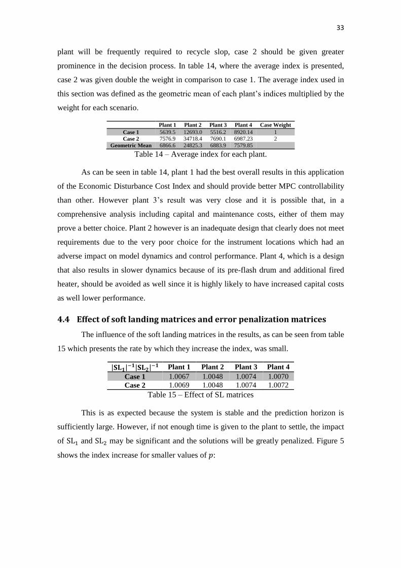
plant will be frequently required to recycle slop, case 2 should be given greater

prominence in the decision process. In table 14, where the average index is presented,

case 2 was given double the weight in comparison to case 1. The average index used in

this section was defined as the geometric mean of each plant’s indices multiplied by the

weight for each scenario.

Plant 1 Plant 2 Plant 3 Plant 4 Case Weight

Case 1 5639.5 12693.0 5516.2 8920.14 1

Case 2 7576.9 34718.4 7690.1 6987.23 2

Geometric Mean 6866.6 24825.3 6883.9 7579.85

Table 14 – Average index for each plant.

As can be seen in table 14, plant 1 had the best overall results in this application

of the Economic Disturbance Cost Index and should provide better MPC controllability

than other. However plant 3’s result was very close and it is possible that, in a

comprehensive analysis including capital and maintenance costs, either of them may

prove a better choice. Plant 2 however is an inadequate design that clearly does not meet

requirements due to the very poor choice for the instrument locations which had an

adverse impact on model dynamics and control performance. Plant 4, which is a design

that also results in slower dynamics because of its pre-flash drum and additional fired

heater, should be avoided as well since it is highly likely to have increased capital costs

as well lower performance.

4.4 Effect of soft landing matrices and error penalization matrices

The influence of the soft landing matrices in the results, as can be seen from table

15 which presents the rate by which they increase the index, was small.

|𝐒𝐋𝟏|−𝟏|𝐒𝐋𝟐|

−𝟏 Plant 1 Plant 2 Plant 3 Plant 4

Case 1 1.0067 1.0048 1.0074 1.0070

Case 2 1.0069 1.0048 1.0074 1.0072

Table 15 – Effect of SL matrices

This is as expected because the system is stable and the prediction horizon is

sufficiently large. However, if not enough time is given to the plant to settle, the impact

of SL1 and SL2 may be significant and the solutions will be greatly penalized. Figure 5

shows the index increase for smaller values of 𝑝:

34

Figure 5 – |SL1|−1|SL2|

−1 for plant 1, scenario 1, for various values of 𝑝.

Since this work is a steady-state focused analysis, the inclusion of SL matrices can

be considered a cautionary measure to ensure validity of the results and force the

optimization algorithm to disregard oscillatory or overshooting solutions if

possible. However, in some design cases the speed of dynamic response may be key and

thus it may be necessary to assess the system thoroughly by testing several different

values for 𝑝.

The identity matrix was always used for the error penalization matrix - which

means no bound violations are permitted during the transients – with the exception of

plant 2 in scenario 2 where |𝐸𝑃|−1 = 1.0104 to allow 𝑦1 < 𝑦𝑚𝑖𝑛,1 over the whole

predicted range.

5 Quantifying the Effects of Model Uncertainty

When designing control systems for robust performance, it is necessary to address

model uncertainty. Similarly, when performing controllability analysis the evaluation of

plant performance should be robust to uncertainty in the model parameters. If the

flowsheets being assessed have very different uncertainty levels in their models,

conducting integrated design and control analysis using only the nominal model will

eventually lead to wrong conclusions.

In this section model uncertainty is embedded in the Economic MPC Optimisation

Index. As discussed in section 3.2 and also in the appendix, the state-space model used in

this paper is derived from transfer function models identified from process simulation

35

data. Thus, the state-space model of each CV/MV pair inherited the same level of

uncertainty of the transfer function from which it is derived.

We shall now define a model uncertainty measure suitable to represent process

nonlinearity. Since simulation is the source of process data in the current work, and for

this reason there are no sensor related issues, model nonlinearity is the major source of

modelling error (numerical error being the remaining possibility). Since step tests are the

chosen method of system identification, we are interested in knowing the magnitude of

uncertainty in the steady-state output change in response to a control action, as shown in

figure 6:

Figure 6 – Uncertainty in the magnitude of the output steady-state change, given

a certain input change.

Let us assume that, for each input/output pair, the test used to identify the linear

model consists of a series of 𝑛 = 1,… ,𝑁𝑠 steps. After the nominal model is identified,

we may validate it by comparing its response to the identification data, thereby obtaining

the model mismatch relative to each one of the steps performed. The model mismatch

value can be positive or negative, and so can step response amplitude. The relative model

mismatch of the nth step, 𝜑𝑛, which relates absolute mismatch to response amplitude, can

be obtained using equation 23:

𝜑𝑛 = (∆𝑦𝑠𝑛 − ∆𝑦𝑛𝑜𝑛,𝑠𝑛) ∆𝑦𝑠𝑛⁄ = 𝑒𝑠𝑛 ∆𝑦𝑠𝑛⁄ (23)

where ∆𝑦𝑠𝑛 is the steady-state response amplitude of plant data relative to the nth

step, ∆𝑦𝑛𝑜𝑛,𝑠𝑛 is the steady-state response amplitude of the nominal model relative to the

nth step, and 𝑒𝑠𝑖 is the steady-state absolute value of model mismatch, also relative to the

nth step. Figure 7 illustrates this concept for a model identification test consisting of 𝑁𝑠 =

3 steps:

36

Figure 7 – Representation of model mismatch for a step test.

It is important to consider that, if the output/input pair is weakly related, the

denominator in equation 23 is small and 𝜑 might become too large (>1). In this case the

control engineer should ignore uncertainty for this 𝑦/𝑢 pair and set 𝜑𝑛 = 0 for 𝑛 =

1, … , 𝑁𝑠. It is important to notice that models can be biased to a particular direction, e.g.,

providing always smaller changes in output prediction than plant data, consistently

resulting in negative model mismatch. Or, alternatively, prediction error may be randomly

distributed, with a similar number of steps with positive and negative model mismatch.

For this reason, equations 24 and 25 define 𝛽𝑦𝑖,𝑢𝑗− and 𝛽𝑦𝑖,𝑢𝑗

+ , respectively the minimum

negative relative model mismatch and the maximum positive relative model mismatch

between 𝑦𝑖 and 𝑢𝑗:

𝛽𝑦𝑖,𝑢𝑗− = 𝑚𝑖𝑛

𝑛=1,…,𝑁𝑠𝜇𝑛 𝜑𝑛, 𝑖 = 1,… , 𝑛𝑦, 𝑗 = 1, … , 𝑛𝑢 (24)

𝛽𝑦𝑖,𝑢𝑗+ = 𝑚𝑎𝑥

𝑛=1,…,𝑁𝑠𝜗𝑛 𝜑𝑛, 𝑖 = 1,… , 𝑛𝑦, 𝑗 = 1,… , 𝑛𝑢 (25)

where 𝜇𝑛 = 1 and 𝜗𝑛 = 0 if 𝜑𝑛 < 0, 𝜇𝑛 = 0 and 𝜗𝑛 = 1 if 𝜑𝑛 > 0, 𝑁𝑠 is again

the number of steps, and 𝑛𝑦 and 𝑛𝑢 are respectively the number of CVs and MVs.

Parameters 𝛽𝑦𝑖,𝑢𝑗− and 𝛽𝑦𝑖,𝑢𝑗

+ may be understood as fractions of the nominal model

response. Similarly, βyi,dj− and βyi,dj

+ are respectively the minimum negative and the

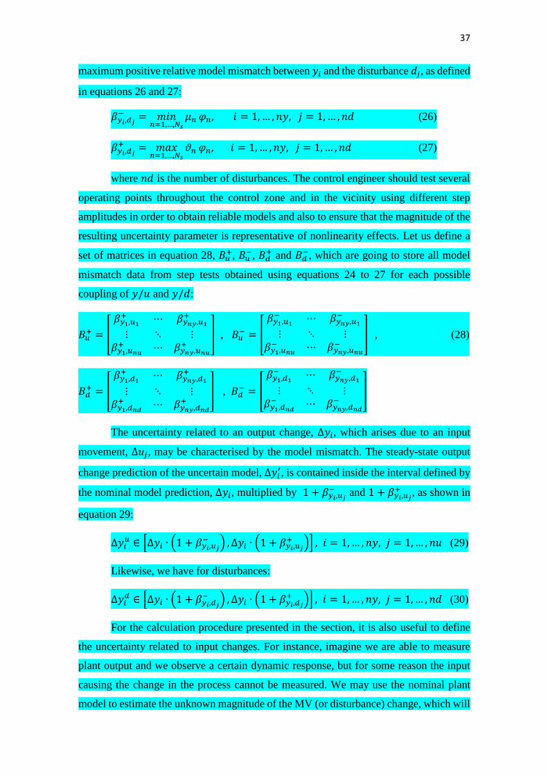
37

maximum positive relative model mismatch between 𝑦𝑖 and the disturbance 𝑑𝑗, as defined

in equations 26 and 27:

𝛽𝑦𝑖,𝑑𝑗− = 𝑚𝑖𝑛

𝑛=1,…,𝑁𝑠𝜇𝑛 𝜑𝑛, 𝑖 = 1,… , 𝑛𝑦, 𝑗 = 1,… , 𝑛𝑑 (26)

𝛽𝑦𝑖,𝑑𝑗+ = 𝑚𝑎𝑥

𝑛=1,…,𝑁𝑠𝜗𝑛 𝜑𝑛, 𝑖 = 1, … , 𝑛𝑦, 𝑗 = 1,… , 𝑛𝑑 (27)

where 𝑛𝑑 is the number of disturbances. The control engineer should test several

operating points throughout the control zone and in the vicinity using different step

amplitudes in order to obtain reliable models and also to ensure that the magnitude of the

resulting uncertainty parameter is representative of nonlinearity effects. Let us define a

set of matrices in equation 28, 𝛣𝑢+, 𝛣𝑢

−, 𝛣𝑑+ and 𝛣𝑑

−, which are going to store all model

mismatch data from step tests obtained using equations 24 to 27 for each possible

coupling of 𝑦/𝑢 and 𝑦/𝑑:

𝛣𝑢+ = [

𝛽𝑦1,𝑢1+ ⋯ 𝛽𝑦𝑛𝑦,𝑢1

+

⋮ ⋱ ⋮𝛽𝑦1,𝑢𝑛𝑢+ ⋯ 𝛽𝑦𝑛𝑦,𝑢𝑛𝑢

+] , 𝛣𝑢

− = [

𝛽𝑦1,𝑢1− ⋯ 𝛽𝑦𝑛𝑦,𝑢1

−

⋮ ⋱ ⋮𝛽𝑦1,𝑢𝑛𝑢− ⋯ 𝛽𝑦𝑛𝑦,𝑢𝑛𝑢

−] , (28)

𝛣𝑑+ = [

𝛽𝑦1,𝑑1+ ⋯ 𝛽𝑦𝑛𝑦,𝑑1

+

⋮ ⋱ ⋮𝛽𝑦1,𝑑𝑛𝑑+ ⋯ 𝛽𝑦𝑛𝑦,𝑑𝑛𝑑

+] , 𝛣𝑑

− = [

𝛽𝑦1,𝑑1− ⋯ 𝛽𝑦𝑛𝑦,𝑑1

−

⋮ ⋱ ⋮𝛽𝑦1,𝑑𝑛𝑑− ⋯ 𝛽𝑦𝑛𝑦,𝑑𝑛𝑑

−]

The uncertainty related to an output change, ∆𝑦𝑖, which arises due to an input

movement, ∆𝑢𝑗, may be characterised by the model mismatch. The steady-state output

change prediction of the uncertain model, ∆𝑦𝑖′, is contained inside the interval defined by

the nominal model prediction, ∆𝑦𝑖, multiplied by 1 + 𝛽𝑦𝑖,𝑢𝑗− and 1 + 𝛽𝑦𝑖,𝑢𝑗

+ , as shown in

equation 29:

∆𝑦𝑖𝑢 ∈ [∆𝑦𝑖 ∙ (1 + 𝛽𝑦𝑖,𝑢𝑗

− ) , ∆𝑦𝑖 ∙ (1 + 𝛽𝑦𝑖,𝑢𝑗+ )] , 𝑖 = 1,… , 𝑛𝑦, 𝑗 = 1,… , 𝑛𝑢 (29)

Likewise, we have for disturbances:

∆𝑦𝑖𝑑 ∈ [∆𝑦𝑖 ∙ (1 + 𝛽𝑦𝑖,𝑑𝑗

− ) , ∆𝑦𝑖 ∙ (1 + 𝛽𝑦𝑖,𝑑𝑗+ )] , 𝑖 = 1,… , 𝑛𝑦, 𝑗 = 1,… , 𝑛𝑑 (30)

For the calculation procedure presented in the section, it is also useful to define

the uncertainty related to input changes. For instance, imagine we are able to measure

plant output and we observe a certain dynamic response, but for some reason the input

causing the change in the process cannot be measured. We may use the nominal plant

model to estimate the unknown magnitude of the MV (or disturbance) change, which will

38

be contained in the value interval ∆𝑢𝑗′ (or ∆𝑑𝑗

′), in a similar way to ∆𝑦𝑖′. This concept is

shown in figure 8:

Figure 8 – Uncertainty in the magnitude of an unknown input change, given a

certain output change.

Now this concept of uncertainty is clearly defined and we have the understanding

that it describes input and output rates of change and not absolute values. Given this

uncertainty definition, if a linear continuous-time state-space model is being used, there

is a relation of proportionality between ∆yiu/∆yi and ∆uj

′/∆uj, and also between ∆yid/∆yi

and ∆dj′/∆dj.

This proportionality also applies to the bound definition of uncertainty intervals

(equations 29 and 30). Due to model linearity, if we multiply an MV change, ∆𝑢𝑗, by any

real number contained in [1 + 𝛽𝑦𝑖,𝑢𝑗− , 1 + 𝛽𝑦𝑖,𝑢𝑗

+ ], the resulting output change will be

contained inside ∆𝑦𝑖𝑢. Similarly, multiplying a disturbance change, ∆𝑑𝑗, by any real

number contained in [1 + 𝛽𝑦𝑖,𝑑𝑗− , 1 + 𝛽𝑦𝑖,𝑑𝑗

+ ], the resulting output change will be contained

inside ∆𝑦𝑖𝑑. We use this effect to obtain equations 31 and 32, which are respectively the

interval of control action magnitude of the uncertain model, ∆𝑢𝑗′, and the interval of

disturbance magnitude of the uncertain model, ∆𝑑𝑗′:

∆𝑢𝑗′ ∈ [∆𝑢𝑗 ∙ (1 + 𝛽𝑦𝑖,𝑢𝑗

− ) , ∆𝑢𝑗 ∙ (1 + 𝛽𝑦𝑖,𝑢𝑗+ )] , 𝑖 = 1,… , 𝑛𝑦, 𝑗 = 1,… , 𝑛𝑢 (31)

∆𝑑𝑗′ ∈ [∆𝑑𝑗 ∙ (1 + 𝛽𝑦𝑖,𝑑𝑗

− ) , ∆𝑑𝑖 ∙ (1 + 𝛽𝑦𝑖,𝑑𝑗+ )] , 𝑖 = 1, … , 𝑛𝑦, 𝑗 = 1, … , 𝑛𝑑 (32)

Let us define two new variables, the uncertainty parameters 𝛾𝑦𝑖,𝑢𝑗 and 𝛾𝑦𝑖,𝑑𝑗, which

are real numbers that can assume any value inside the limits defined by, respectively,

[1 + 𝛽𝑦𝑖,𝑢𝑗− , 1 + 𝛽𝑦𝑖,𝑢𝑗

+ ] and [1 + 𝛽𝑦𝑖,𝑑𝑗− , 1 + 𝛽𝑦𝑖,𝑑𝑗

+ ], as shown in equations 33 and 34:

𝛾𝑦𝑖𝑢𝑗 ∈ [1 + 𝛽𝑦𝑖,𝑢𝑗− , 1 + 𝛽𝑦𝑖,𝑢𝑗

+ ] (33)

𝛾𝑦𝑖𝑑𝑗 ∈ [1 + 𝛽𝑦𝑖,𝑑𝑗− , 1 + 𝛽𝑦𝑖,𝑑𝑗

+ ] (34)

39

Equation 3, which calculates the output prediction of the nominal model, can be

modified to incorporate these new variables, obtaining new output trajectories as the

uncertainty parameters assume different values. In order to do that, instead of applying

the original MV change ∆uk at time k, we apply γyiuj∆uk, where i = 1, …ny, j = 1,… nu.

At time k + 1 we apply γyiuj∆uk+1 instead of ∆uk+1, and so forth until the end of the

control horizon, k + m. The same approach can be used for disturbances. We replace ∆dk

for γyidj∆dk at time k, where i = 1,… ny, j = 1,… nd, and then replace ∆dk+1 for

γyidj∆dk+1 at time k + 1, and proceed likewise all the way until the end of the prediction

horizon, k + p. These substitutions yield equation 35, enabling us to calculate a new

output prediction of the uncertain model, y ,, where y, ∈ (∆yu⋃∆yd).

𝑦𝑘+1, = 𝐶𝑥𝑘+1 = 𝐶𝐴𝑥𝑘 + 𝑑𝑖𝑎𝑔(𝐶𝐵𝛤𝛥𝑢𝑘) + 𝑑𝑖𝑎𝑔(𝐶𝐵𝛤𝛥𝑑𝑘)

𝑦𝑘+2, = 𝐶𝑥𝑘+2 = 𝐶𝐴𝑥𝑘+1 + 𝑑𝑖𝑎𝑔(𝐶𝐵𝛤𝛥𝑢𝑘+1) + 𝑑𝑖𝑎𝑔(𝐶𝐵𝛤𝛥𝑑𝑘+1)

= 𝐶𝐴2𝑥𝑘 + 𝑑𝑖𝑎𝑔 ([𝐶𝐴𝐵 𝐶𝐵] [𝛤𝛥𝑢𝑘𝛤𝛥𝑢𝑘+1

]) + 𝑑𝑖𝑎𝑔 ([𝐶𝐴𝐷 𝐶𝐷] [𝛤𝛥𝑑𝑘𝛤𝛥𝑑𝑘+1

]) (35)

⋮

𝑦𝑘+𝑝, = 𝐶𝐴𝑝𝑥𝑘 + 𝑑𝑖𝑎𝑔 ([𝐶𝐴

𝑝−1𝐵 𝐶𝐴𝑝−2𝐵 … 𝐶𝐴𝑝−𝑚𝐵][𝛤𝛥𝑢𝑘 𝛤𝛥𝑢𝑘+1 … 𝛤𝛥𝑢𝑘+𝑚−1]𝑇)

+𝑑𝑖𝑎𝑔 ([𝐶𝐴𝑝−1𝐷 𝐶𝐴𝑝−2𝐷 … 𝐶𝐴2𝐷] [𝛤𝛥𝑑𝑘 𝛤𝛥𝑑𝑘+1 … 𝛤𝛥𝑑𝑘+𝑝−3]𝑇

)

where:

𝛤𝛥𝑢𝑘+𝜎,𝜎=0,…,𝑚−1 =

[ 𝛾𝑦1𝑢1∆𝑢𝑘+𝜎,1 𝛾𝑦2𝑢1∆𝑢𝑘+𝜎,1 ⋯

𝛾𝑦1𝑢2∆𝑢𝑘+𝜎,2 𝛾𝑦2𝑢2∆𝑢𝑘+𝜎,2 ⋯

⋮ ⋮ ⋱

𝛾𝑦𝑛𝑦𝑢1∆𝑢𝑘+𝜎,1

𝛾𝑦𝑛𝑦𝑢2∆𝑢𝑘+𝜎,2⋮

𝛾𝑦1𝑢𝑛𝑢∆𝑢𝑘+𝜎,𝑛𝑢 𝛾𝑦2𝑢𝑛𝑢∆𝑢𝑘+𝜎,𝑛𝑢 ⋯ 𝛾𝑦𝑛𝑦𝑢𝑛𝑢∆𝑢𝑘+𝜎,𝑛𝑢]

𝛤𝛥𝑑𝑘+𝜎,𝜎=0,…,𝑝−3 =

[ 𝛾𝑦1𝑑1∆𝑑𝑘+𝜎,1 𝛾𝑦2𝑑1∆𝑑𝑘+𝜎,1 ⋯

𝛾𝑦1𝑑2∆𝑑𝑘+𝜎,2 𝛾𝑦2𝑑2∆𝑑𝑘+𝜎,2 ⋯

⋮ ⋮ ⋱

𝛾𝑦𝑛𝑦𝑑1∆𝑑𝑘+𝜎,1

𝛾𝑦𝑛𝑦𝑑2∆𝑑𝑘+𝜎,2⋮

𝛾𝑦1𝑑𝑛𝑑∆𝑑𝑘+𝜎,𝑛𝑑 𝛾𝑦2𝑑𝑛𝑑∆𝑑𝑘+𝜎,𝑛𝑑 ⋯ 𝛾𝑦𝑛𝑦𝑑𝑛𝑑∆𝑑𝑘+𝜎,𝑛𝑑]

The Economic MPC Optimisation Index procedure will be now updated to

incorporate model uncertainty. Since equation 35 may be used to obtain the feasible

intervals of predictions, the optimisation problem can be modified to provide a multilayer

optimisation problem, enabling us to calculate the “worst” and “best” possible model

indices. The first step of the new procedure is to solve the nominal model problem

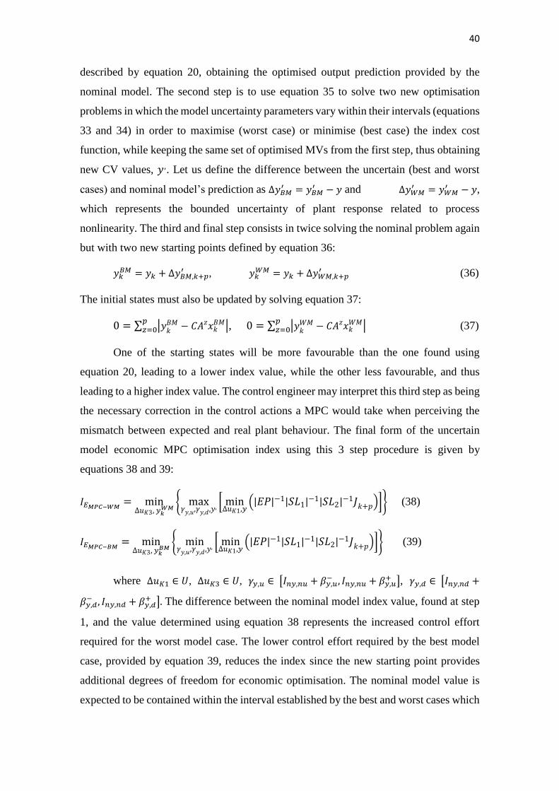
40

described by equation 20, obtaining the optimised output prediction provided by the

nominal model. The second step is to use equation 35 to solve two new optimisation

problems in which the model uncertainty parameters vary within their intervals (equations

33 and 34) in order to maximise (worst case) or minimise (best case) the index cost

function, while keeping the same set of optimised MVs from the first step, thus obtaining

new CV values, 𝑦 ,. Let us define the difference between the uncertain (best and worst

cases) and nominal model’s prediction as ∆𝑦𝐵𝑀′ = 𝑦𝐵𝑀

′ − 𝑦 and ∆𝑦𝑊𝑀′ = 𝑦𝑊𝑀

′ − 𝑦,

which represents the bounded uncertainty of plant response related to process

nonlinearity. The third and final step consists in twice solving the nominal problem again

but with two new starting points defined by equation 36:

𝑦𝑘𝐵𝑀 = 𝑦𝑘 + ∆𝑦𝐵𝑀,𝑘+𝑝

′ , 𝑦𝑘𝑊𝑀 = 𝑦𝑘 + ∆𝑦𝑊𝑀,𝑘+𝑝

′ (36)

The initial states must also be updated by solving equation 37:

0 = ∑ |𝑦𝑘𝐵𝑀 − 𝐶𝐴𝑧𝑥𝑘

𝐵𝑀|𝑝𝑧=0 , 0 = ∑ |𝑦

𝑘𝑊𝑀 − 𝐶𝐴𝑧𝑥𝑘

𝑊𝑀|𝑝𝑧=0 (37)

One of the starting states will be more favourable than the one found using

equation 20, leading to a lower index value, while the other less favourable, and thus

leading to a higher index value. The control engineer may interpret this third step as being

the necessary correction in the control actions a MPC would take when perceiving the

mismatch between expected and real plant behaviour. The final form of the uncertain

model economic MPC optimisation index using this 3 step procedure is given by

equations 38 and 39:

𝐼𝐸𝑀𝑃𝐶−𝑊𝑀 = min∆𝑢𝐾3, 𝑦𝑘

𝑊𝑀{ max𝛾𝑦,𝑢,𝛾𝑦,𝑑,𝑦

,[ min∆𝑢𝐾1,𝑦

(|𝐸𝑃|−1|𝑆𝐿1|−1|𝑆𝐿2|

−1𝐽𝑘+𝑝)]} (38)

𝐼𝐸𝑀𝑃𝐶−𝐵𝑀 = min∆𝑢𝐾3, 𝑦𝑘

𝐵𝑀{ min𝛾𝑦,𝑢,𝛾𝑦,𝑑,𝑦

,[ min∆𝑢𝐾1,𝑦

(|𝐸𝑃|−1|𝑆𝐿1|−1|𝑆𝐿2|

−1𝐽𝑘+𝑝)]} (39)

where ∆𝑢𝐾1 ∈ 𝑈, ∆𝑢𝐾3 ∈ 𝑈, 𝛾𝑦,𝑢 ∈ [𝐼𝑛𝑦,𝑛𝑢 + 𝛽𝑦,𝑢− , 𝐼𝑛𝑦,𝑛𝑢 + 𝛽𝑦,𝑢

+ ], 𝛾𝑦,𝑑 ∈ [𝐼𝑛𝑦,𝑛𝑑 +

𝛽𝑦,𝑑− , 𝐼𝑛𝑦,𝑛𝑑 + 𝛽𝑦,𝑑

+ ]. The difference between the nominal model index value, found at step

1, and the value determined using equation 38 represents the increased control effort

required for the worst model case. The lower control effort required by the best model

case, provided by equation 39, reduces the index since the new starting point provides

additional degrees of freedom for economic optimisation. The nominal model value is

expected to be contained within the interval established by the best and worst cases which

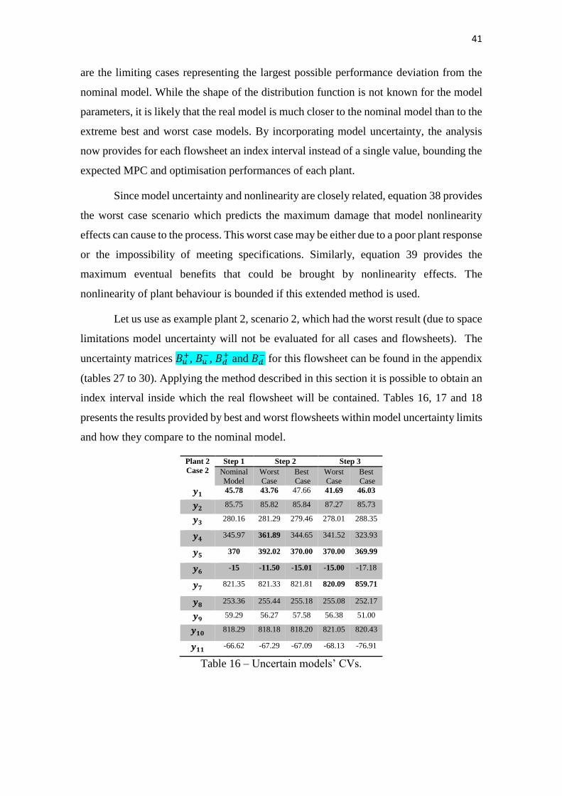
41

are the limiting cases representing the largest possible performance deviation from the

nominal model. While the shape of the distribution function is not known for the model

parameters, it is likely that the real model is much closer to the nominal model than to the

extreme best and worst case models. By incorporating model uncertainty, the analysis

now provides for each flowsheet an index interval instead of a single value, bounding the

expected MPC and optimisation performances of each plant.

Since model uncertainty and nonlinearity are closely related, equation 38 provides

the worst case scenario which predicts the maximum damage that model nonlinearity

effects can cause to the process. This worst case may be either due to a poor plant response

or the impossibility of meeting specifications. Similarly, equation 39 provides the

maximum eventual benefits that could be brought by nonlinearity effects. The

nonlinearity of plant behaviour is bounded if this extended method is used.

Let us use as example plant 2, scenario 2, which had the worst result (due to space

limitations model uncertainty will not be evaluated for all cases and flowsheets). The

uncertainty matrices 𝛣𝑢+, 𝛣𝑢

−, 𝛣𝑑+ and 𝛣𝑑

− for this flowsheet can be found in the appendix

(tables 27 to 30). Applying the method described in this section it is possible to obtain an

index interval inside which the real flowsheet will be contained. Tables 16, 17 and 18

presents the results provided by best and worst flowsheets within model uncertainty limits

and how they compare to the nominal model.

Plant 2

Case 2

Step 1 Step 2 Step 3

Nominal

Model

Worst

Case

Best

Case

Worst

Case

Best

Case

𝒚𝟏 45.78 43.76 47.66 41.69 46.03

𝒚𝟐 85.75 85.82 85.84 87.27 85.73

𝒚𝟑 280.16 281.29 279.46 278.01 288.35

𝒚𝟒 345.97 361.89 344.65 341.52 323.93

𝒚𝟓 370 392.02 370.00 370.00 369.99

𝒚𝟔 -15 -11.50 -15.01 -15.00 -17.18

𝒚𝟕 821.35 821.33 821.81 820.09 859.71

𝒚𝟖 253.36 255.44 255.18 255.08 252.17

𝒚𝟗 59.29 56.27 57.58 56.38 51.00

𝒚𝟏𝟎 818.29 818.18 818.20 821.05 820.43

𝒚𝟏𝟏 -66.62 -67.29 -67.09 -68.13 -76.91

Table 16 – Uncertain models’ CVs.

42

Plant 2

Case 2

Step 1/2 Step 3

Nominal

Model

Worst

Case

Best

Case

𝒖𝟏 40.00 40.00 67.94

𝒖𝟐 320.00 320.00 332.24

𝒖𝟑 154.92 170.02 72.77

𝒖𝟒 0.03 12.29 59.91

𝒖𝟓 23.59 52.76 261.59

𝒖𝟔 686.41 657.24 434.29

𝒖𝟕 0.00 0.00 14.11

𝒅𝟏 90.00 90.00 90.00

Table 17 – Uncertain models’ MVs

Plant 2 Nominal

Model

Best

Model

Worst

Model

Case 2 – Step 3 34,718.4 16,744.0 4,342,402.4

Table 18 – Uncertain models’ indices

These tables show that inside the range of uncertainty parameters obtained

through model identification for plant 2, there is a best possible model that would be

capable of producing diesel within specification, something that the nominal plant 2 is

not capable of accomplishing. The worst case plant is much further away from acceptable

performance than the nominal plant. For the worst-case plant 2, there is no opportunity

for acceptable MPC performance – a MPC package capable of delivering good

performance does not exist since it is not achievable for these conditions.

The best and worst case models are situated at the extremes of model uncertainty

and thus are highly unlikely, if not impossible, to be true. If the user is willing to adopt a

less rigorous approach in order to obtain a more meaningful index interval, one should

consider using the standard deviation of negative and positive relative model mismatches

to calculate parameters 𝛽𝑦,𝑢+ , 𝛽𝑦,𝑢

− , 𝛽𝑦,𝑑+ and 𝛽𝑦,𝑑

− instead of respectively minimum and

maximum values. The interval thus obtained might enable better comparison between

plants.

6 Conclusions and Future work

The work presented a new method to assess the expected controllability, control

resilience and profitability of chemical plants where zone constrained or traditional model

predictive control is to be used. Here we have used models derived from simulation step

43

tests to aid practical implementation and hence encourage its use. A new economic cost

index which included elements of controller performance has been developed which

enables us to compare designs. The index includes constraint violations, enforcing for

hard constraints but allowing some leniency where necessary for soft constraints, and

smoothness of response. Best and worst case bounds can be obtained to allow for

nonlinearity of the system. The approach has been demonstrated on a problem of

considerable complexity, a crude distillation system.

When making use of linear models it is assumed that the process is nearly linear,

at least locally, otherwise the model would be invalid when the present values for the

variables are too distant from the base case where the model parameters were obtained.

Some error due to linearisation can be tolerated but it is necessary to assess whether or

not it compromises the whole analysis. If the assumption of a linear model derived from

process simulation is reasonably valid within the zone constraints of the control problem,

it won’t compromise the use of the economic MPC optimization index as presented here.

However, we have provided a method for quantifying the effects of model nonlinearity

and uncertainty on the index and obtaining an index interval that bounds plant

performance.

Nonlinearity effects tend to affect the dynamic response of different flowsheets in

a similar way. In particular, the final steady state usually moves in the same direction. For

instance consider figure 6 where we compare the diesel flash point (𝑦2) dynamic response

for the base and pre-flash plants, following an increase in medium crude oil flow rate

(∆𝑢5 = +20 𝑚3). In case 1, both plants were processing a heavy mix of crude oil at a

high furnace outlet temperature, whereas in case 2 both plants operated with a much

lighter oil mix at low outlet temperature. Due to process nonlinearity, the significant

change in operating starting point in effect modified by some degree the size of decrease

in 2y . However the changes were in the same direction (a lower decrease in case 2 relative

to case 1 for both plants). Since all plants are similarly affected by changes in operating

point and the effects of nonlinearity, they produce smaller changes in the final results and

the analysis done with linear models should remain valid unless differences in the index’s

scores are very small. MPC packages in industrial applications make successful use of

linear models, showing that most of the time these effects can be ignored for control

purposes.

44

Figure 6 – Comparing nonlinearity for 2 different plants.

Future work will develop a multi-model approach where multiple linear models

with different validity zones are used. The use of nonlinear state-space models based on

phenomenological models and infinite prediction horizon will also be explored. The

downside of these alternatives would likely be the increased computational costs which

will reduce the range of processes for which the approach can be applied.

At the time of writing, even when linear models are used, solving the economic

MPC optimisation index involves significant computational cost when dealing with

complex systems. For example, the problem described in section 3 and 4 was solved using

MATLAB® R2014a running on a 3GHz quad-core Intel Xeon E5-1607 CPU, of which

50% of its capacity was available to the solver. Each iteration takes between 25 and 45

minutes. The computational demand can be much reduced by using smaller control or

prediction horizons, 𝑚 and 𝑝. Using 𝑚 = 1 reduces the computing time necessary to each

iteration to only 3-5 minutes. However it is recommend to set 𝑚 as high as possible,

enabling additional degrees of freedom for the algorithm, which in turn leads to less

conservative control actions. On the other hand, 𝑘 only needs to be high enough to

compute the whole transient prediction.

Acknowledgement

45

The authors thank CAPES and Brazil’s Ministry of Education for the financial

support and scholarship, and Petrobras and University College London for the

encouragement received.

References

Adetola V, Guay M. Integration of real time optimization and model predictive control.

Journal of Process Control 2010;20:125–33.

Alhammadi H, Romagnoli J. Process Design and Operation: Incorporating

Environmental, Profitability, Heat Integration and Controllability Considerations.

The Integration of Process Design and Control 2004;17:264-306.

Alvarado-Morales M, Abd Hamid MK, Sin G, Gernaey KV, Woodley JM, Gani R. A

model-based methodology for simultaneous design and control of a bioethanol

production process. Comput Chen Eng 2010;34:2043–61.

Amrit R, Rawlings JB, Biegler LT. Optimizing process economics online using model

predictive control. Comput Chem Eng 2013;58:334–43.

Bahakim SS, Ricardez-Sandoval LA. Simultaneous design and MPC-based control for

dynamic systems under uncertainty: A stochastic approach. Comput Chem Eng

2014;63:66–81.

Bansal V, Perkins JD, Pistikopoulos EN. A Case Study in Simultaneous Design and

Control Using Rigorous, Mixed-Integer Dynamic Optimization Models. Ind Eng

Chem Res 2002;41:760–78.

Bansal V, Ross R, Perkins JD, Pistikopoulos EN. The interactions of design and control:

double-effect distillation. J Process Contr 2000;10:219–27.

Bemporad A, Morari M. Robust model predictive control: A survey, Lecture Notes in

Control and Information Sciences 1999;245:207–226.

Brengel DD, Seider W. Coordinated design and control optimization of nonlinear

processes, Chem Eng Com 1992;16:861–86.

Chawankul N, Ricardez-Sandoval LA, Budman H, Douglas PL. Integration of Design

and Control: A Robust Control Approach Using MPC. The Canadian Journal of

Chemical Engineering 2007;85(4):433–46.

Ferramosca A, Gonzalez AH, Limon D, Odloak D. One-layer robust MPC: a multi-

model approach. Preprints of the 19th World Congress, The International Federation

of Automatic Control, Cape Town, South Africa. August 24-29, 2014.

Francisco M, Vega P, Alvarez H. Robust integrated design of process with terminal

penalty model predictive controllers. Ind Eng Chem Res 2011;89:1011−24.

González AH, Marchetti JL, Odloak D. Extended Robust Model Predictive Control of

Integrating Systems. AIChE J 2007;53(7):1758–69.

González AH, Odloak D. A stable MPC with zone control. Journal of Process Control

2009;19(1):110–122.

Gouvêa MT, Odloak D. One-layer real time optimization of LPG production in the FCC

unit: Procedure, advantages and disadvantages. Comput Chem Eng 1998;22:191–98.

46

Grosman B, Dassau E, Zisser HC, Jovanovič L, Doyle III FJ. Zone Model Predictive

Control: A Strategy to Minimize Hyper- and Hypoglycemic Events. Journal of

Diabetes Science and Technology 2010;4(4).

Lewin DR. A Simple Tool for Disturbance Resiliency Diagnosis and Feedforward

Control Design. Comput Chem Eng 1996; 20:13.

Luo X, Zhou X, Wang S, Xu F. Zone Control with Model Predictive Control for Much

Constrained States Process. Proceedings of the 31st Chinese Control Conference, July

25-27, 2012, Hefei, China.

Martins MAF, Yamashita AS, Santoro BF, Odloak D. Robust model predictive control

of integrating time delay processes. Journal of Process Control 2013;23:917–32.

Mayne DQ, Rawlings JB, Rao CV, Scokaert POM. Constrained Model Predictive

Control: Stability and Optimality. Automatica 2000; 36:789.

Mohideen MJ, Perkins JD, Pistikopoulos EN. Optimal design of dynamic systems under

uncertainty. AIChE Journal 1996;42(8):2251–72.

Oliveira MC, Bernussou J, Geromel JC. A new discrete-time robust stability condition.

Systems & Control Letters 1999;37:261–65.

Perkins JD, Walsh SPK. Optimization as a tool for design/control integration. Comput

Chem Eng 1996;20(4):315–23.

Porfírio CR, Odloak D. Optimizing model predictive control of an industrial distillation

column, Control Engineering Practice 2011;19(10):1137–46.

Ricardez-Sandoval LA, Budman H, Douglas P. Integration of Design and Control for

Chemical Processes: A Review of the Literature and Some Recent Results. Annual

Reviews in Control 2009;33(2):158-71.

Ricardez-Sandoval LA, Douglas PL, Budman HM. A methodology for the simultaneous

design and control of large-scale systems under process parameter uncertainty.

Comput Chen Eng 2011;35:307–18.

Rodrigues MA, Odloak D. Output feedback MPC with guaranteed robust stability.

Journal of Process Control 2000;10:557–72.

Sakizlis V, Perkins JD, Pistikopoulos EN. Recent advances in optimization-based

simultaneous process and control design. Comput Chem Eng 2004;28:2069–86.

Sánchez-Sánchez KB, Ricardez-Sandoval LA. Simultaneous design and control under

uncertainty using model predictive control. Ind Eng Chem Res 2013; 52:4815–33.

Sánchez-Sánchez KB, Ricardez-Sandoval LA. Simultaneous process synthesis and

control design under uncertainty: A worst-case performance approach. AIChE J

2013;59(7):2497–2514.

Skogestad S, Morari M. Implications of large RGA-elements on control performance.

Ind Eng Chem Res 1987:26(11):2323–30.

Solovyev BM, Lewin DR. A Steady-state Process Resiliency Index for Non-linear

Processes: 1. Analysis, W. L. Luyben Edition of Ind Eng Chem Res 2002.

Strutzel FAM, Odloak D, Zanin AC. Economic MPC of an Industrial Diesel

Hydrotreating Plant. Proceedings of Intelligent Systems and Control (PE 2013),

November 11 – 13, 2013, Marina del Rey, USA.

47

Trainor M, Giannakeas V, Kiss C, Ricardez-Sandoval, LA. Optimal process and control

design under uncertainty: A methodology with robust feasibility and stability

analyses. Chem Eng Sci 2013;104:1065-80.

Vidyasagar M. Nonlinear Systems Analysis 2nd edition. Society for Industrial and

Applied Mathematics 2002.

Weitz O, Lewin DR. Dynamic controllability and resiliency diagnosis using steady state

process flowsheet data. Comput Chem Eng 1996;20(4):325–35.

Yuan Z, Chen B, Zhao J. An overview on controllability analysis of chemical processes.

AIChE Journal 2011; 57(5):1185–1201.

Zhang X, Luo X, Wang S. The Expression of Control Law for Zone Constraints

Predictive Control. Artificial Intelligence and Computational Intelligence, Second

International Conference, AICI 2011, Taiyuan, China, September 24-25, 2011.

48

Appendix

Continuous-Time Transfer Functions for the Crude Oil Distillation Process

As discussed in section 3.2, this work made use of the output prediction oriented

model (OPOM), a state-space formulation that is built upon the transfer functions that

define the interaction between each pair of manipulated/disturbance and controlled

variable. In order to identify these models, a series of step tests was carried using the

dynamic simulations of the four different designs of the crude oil distillation process

presented in section 4. Tables from 14 to 21 display parameters to be substituted in

equation 19 as a means to represent each model as a 5th order transfer function.

0,,1,,

2

2,,

3

3,,

4

4,,

5

5,,

0,,1,,

2

2,,

3

3,,

4

4,,

5

5,,

, )(jijijijijiji

jijijijijiji

jiasasasasasa

bsbsbsbsbsbsG

(40)

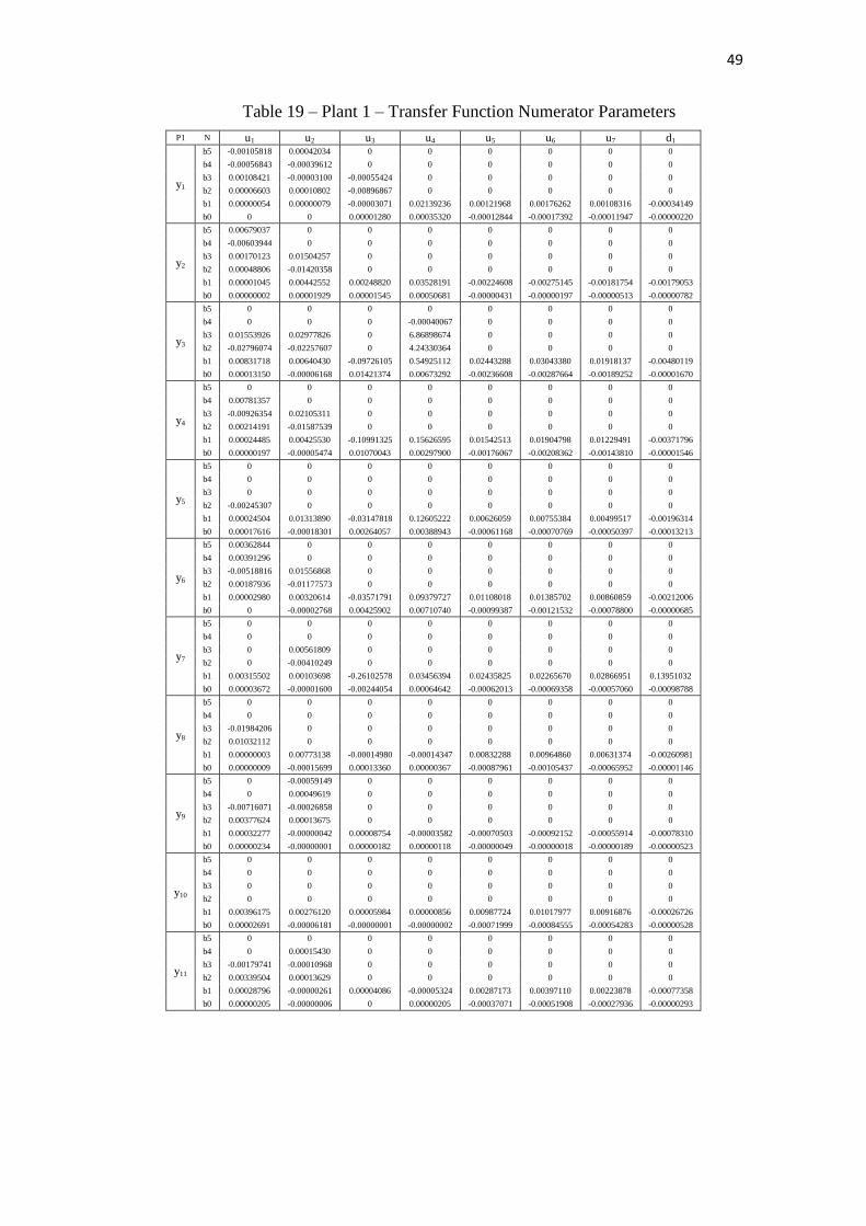
49

Table 19 – Plant 1 – Transfer Function Numerator Parameters

P1 N u1 u2 u3 u4 u5 u6 u7 d1

y1

b5 -0.00105818 0.00042034 0 0 0 0 0 0

b4 -0.00056843 -0.00039612 0 0 0 0 0 0

b3 0.00108421 -0.00003100 -0.00055424 0 0 0 0 0

b2 0.00006603 0.00010802 -0.00896867 0 0 0 0 0

b1 0.00000054 0.00000079 -0.00003071 0.02139236 0.00121968 0.00176262 0.00108316 -0.00034149

b0 0 0 0.00001280 0.00035320 -0.00012844 -0.00017392 -0.00011947 -0.00000220

y2

b5 0.00679037 0 0 0 0 0 0 0

b4 -0.00603944 0 0 0 0 0 0 0

b3 0.00170123 0.01504257 0 0 0 0 0 0

b2 0.00048806 -0.01420358 0 0 0 0 0 0

b1 0.00001045 0.00442552 0.00248820 0.03528191 -0.00224608 -0.00275145 -0.00181754 -0.00179053

b0 0.00000002 0.00001929 0.00001545 0.00050681 -0.00000431 -0.00000197 -0.00000513 -0.00000782

y3

b5 0 0 0 0 0 0 0 0

b4 0 0 0 -0.00040067 0 0 0 0

b3 0.01553926 0.02977826 0 6.86898674 0 0 0 0

b2 -0.02796074 -0.02257607 0 4.24330364 0 0 0 0

b1 0.00831718 0.00640430 -0.09726105 0.54925112 0.02443288 0.03043380 0.01918137 -0.00480119

b0 0.00013150 -0.00006168 0.01421374 0.00673292 -0.00236608 -0.00287664 -0.00189252 -0.00001670

y4

b5 0 0 0 0 0 0 0 0

b4 0.00781357 0 0 0 0 0 0 0

b3 -0.00926354 0.02105311 0 0 0 0 0 0

b2 0.00214191 -0.01587539 0 0 0 0 0 0

b1 0.00024485 0.00425530 -0.10991325 0.15626595 0.01542513 0.01904798 0.01229491 -0.00371796

b0 0.00000197 -0.00005474 0.01070043 0.00297900 -0.00176067 -0.00208362 -0.00143810 -0.00001546

y5

b5 0 0 0 0 0 0 0 0

b4 0 0 0 0 0 0 0 0

b3 0 0 0 0 0 0 0 0

b2 -0.00245307 0 0 0 0 0 0 0

b1 0.00024504 0.01313890 -0.03147818 0.12605222 0.00626059 0.00755384 0.00499517 -0.00196314

b0 0.00017616 -0.00018301 0.00264057 0.00388943 -0.00061168 -0.00070769 -0.00050397 -0.00013213

y6

b5 0.00362844 0 0 0 0 0 0 0

b4 0.00391296 0 0 0 0 0 0 0

b3 -0.00518816 0.01556868 0 0 0 0 0 0

b2 0.00187936 -0.01177573 0 0 0 0 0 0

b1 0.00002980 0.00320614 -0.03571791 0.09379727 0.01108018 0.01385702 0.00860859 -0.00212006

b0 0 -0.00002768 0.00425902 0.00710740 -0.00099387 -0.00121532 -0.00078800 -0.00000685

y7

b5 0 0 0 0 0 0 0 0

b4 0 0 0 0 0 0 0 0

b3 0 0.00561809 0 0 0 0 0 0

b2 0 -0.00410249 0 0 0 0 0 0

b1 0.00315502 0.00103698 -0.26102578 0.03456394 0.02435825 0.02265670 0.02866951 0.13951032

b0 0.00003672 -0.00001600 -0.00244054 0.00064642 -0.00062013 -0.00069358 -0.00057060 -0.00098788

y8

b5 0 0 0 0 0 0 0 0

b4 0 0 0 0 0 0 0 0

b3 -0.01984206 0 0 0 0 0 0 0

b2 0.01032112 0 0 0 0 0 0 0

b1 0.00000003 0.00773138 -0.00014980 -0.00014347 0.00832288 0.00964860 0.00631374 -0.00260981

b0 0.00000009 -0.00015699 0.00013360 0.00000367 -0.00087961 -0.00105437 -0.00065952 -0.00001146

y9

b5 0 -0.00059149 0 0 0 0 0 0

b4 0 0.00049619 0 0 0 0 0 0

b3 -0.00716071 -0.00026858 0 0 0 0 0 0

b2 0.00377624 0.00013675 0 0 0 0 0 0

b1 0.00032277 -0.00000042 0.00008754 -0.00003582 -0.00070503 -0.00092152 -0.00055914 -0.00078310

b0 0.00000234 -0.00000001 0.00000182 0.00000118 -0.00000049 -0.00000018 -0.00000189 -0.00000523

y10

b5 0 0 0 0 0 0 0 0

b4 0 0 0 0 0 0 0 0

b3 0 0 0 0 0 0 0 0

b2 0 0 0 0 0 0 0 0

b1 0.00396175 0.00276120 0.00005984 0.00000856 0.00987724 0.01017977 0.00916876 -0.00026726

b0 0.00002691 -0.00006181 -0.00000001 -0.00000002 -0.00071999 -0.00084555 -0.00054283 -0.00000528

y11

b5 0 0 0 0 0 0 0 0

b4 0 0.00015430 0 0 0 0 0 0

b3 -0.00179741 -0.00010968 0 0 0 0 0 0

b2 0.00339504 0.00013629 0 0 0 0 0 0

b1 0.00028796 -0.00000261 0.00004086 -0.00005324 0.00287173 0.00397110 0.00223878 -0.00077358

b0 0.00000205 -0.00000006 0 0.00000205 -0.00037071 -0.00051908 -0.00027936 -0.00000293

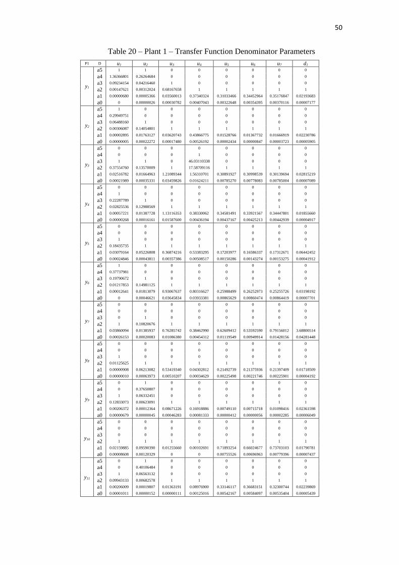
50

Table 20 – Plant 1 – Transfer Function Denominator Parameters

P1 D u1 u2 u3 u4 u5 u6 u7 d1

y1

a5 1 1 0 0 0 0 0 0

a4 1.36366801 0.26264684 0 0 0 0 0 0

a3 0.09234154 0.04216460 1 0 0 0 0 0

a2 0.00147621 0.00312024 0.68167658 1 1 1 1 1

a1 0.00000680 0.00005366 0.03560013 0.37340324 0.31033466 0.34452964 0.35176847 0.02193683

a0 0 0.00000026 0.00030782 0.00407043 0.00322648 0.00354395 0.00370116 0.00007177

y2

a5 1 0 0 0 0 0 0 0

a4 0.29949751 0 0 0 0 0 0 0

a3 0.06488160 1 0 0 0 0 0 0

a2 0.00306087 0.14054801 1 1 1 1 1 1

a1 0.00002895 0.01763127 0.03620743 0.43866775 0.01528766 0.01367732 0.01666919 0.02230786

a0 0.00000005 0.00022272 0.00017480 0.00526192 0.00002434 0.00000847 0.00003723 0.00005905

y3

a5 0 0 0 0 0 0 0 0

a4 0 0 0 1 0 0 0 0

a3 1 1 0 46.03110338 0 0 0 0

a2 0.37554760 0.13570009 1 17.58709116 1 1 1 1

a1 0.02516782 0.01664963 1.21089344 1.56310701 0.30891927 0.30998539 0.30139694 0.02815219

a0 0.00021989 0.00035331 0.03459826 0.01624211 0.00785270 0.00778083 0.00785004 0.00007089

y4

a5 0 0 0 0 0 0 0 0

a4 1 0 0 0 0 0 0 0

a3 0.22287789 1 0 0 0 0 0 0

a2 0.02825536 0.12988569 1 1 1 1 1 1

a1 0.00057221 0.01387728 1.13116353 0.38330062 0.34581491 0.33921567 0.34447801 0.01855660

a0 0.00000268 0.00016161 0.01587600 0.00436194 0.00437167 0.00425213 0.00442939 0.00004917

y5

a5 0 0 0 0 0 0 0 0

a4 0 0 0 0 0 0 0 0

a3 1 0 0 0 0 0 0 0

a2 0.18435735 1 1 1 1 1 1 1

a1 0.03079164 0.05226808 0.36874216 0.53383295 0.17203977 0.16586337 0.17312671 0.06442452

a0 0.00024846 0.00043811 0.00357386 0.00508517 0.00150286 0.00143274 0.00153275 0.00041912

y6

a5 1 0 0 0 0 0 0 0

a4 0.37737981 0 0 0 0 0 0 0

a3 0.19790672 1 0 0 0 0 0 0

a2 0.01217853 0.14981125 1 1 1 1 1 1

a1 0.00012641 0.01813079 0.93067637 0.80316627 0.25988499 0.26252973 0.25255726 0.03198192

a0 0 0.00046621 0.03645834 0.03933381 0.00865629 0.00860474 0.00864419 0.00007701

y7

a5 0 0 0 0 0 0 0 0

a4 0 0 0 0 0 0 0 0

a3 0 1 0 0 0 0 0 0

a2 1 0.10820676 1 1 1 1 1 1

a1 0.03860094 0.01385937 0.76285742 0.38462990 0.62609412 0.53592590 0.79156012 3.68800514

a0 0.00026153 0.00020083 0.01086380 0.00454312 0.01119549 0.00949914 0.01428156 0.04281448

y8

a5 0 0 0 0 0 0 0 0

a4 0 0 0 0 0 0 0 0

a3 1 0 0 0 0 0 0 0

a2 0.01125625 1 1 1 1 1 1 1

a1 0.00000908 0.06213082 0.53419340 0.04302812 0.21492739 0.21375936 0.21397409 0.01718509

a0 0.00000010 0.00063973 0.00510207 0.00034629 0.00225498 0.00221746 0.00225901 0.00004192

y9

a5 0 1 0 0 0 0 0 0

a4 0 0.37650807 0 0 0 0 0 0

a3 1 0.06332451 0 0 0 0 0 0

a2 0.12833073 0.00623091 1 1 1 1 1 1

a1 0.00206372 0.00012364 0.08671226 0.16918886 0.00749110 0.00715718 0.01098416 0.02361598

a0 0.00000679 0.00000045 0.00046283 0.00081333 0.00000412 0.00000056 0.00002285 0.00006049

y10

a5 0 0 0 0 0 0 0 0

a4 0 0 0 0 0 0 0 0

a3 0 0 0 0 0 0 0 0

a2 1 1 1 1 1 1 1 1

a1 0.02159885 0.09590390 0.01255660 0.00102691 0.71893254 0.66024677 0.73703103 0.01790781

a0 0.00008608 0.00120329 0 0 0.00755526 0.00696963 0.00779396 0.00007437

y11

a5 0 1 0 0 0 0 0 0

a4 0 0.40106484 0 0 0 0 0 0

a3 1 0.06563132 0 0 0 0 0 0

a2 0.09943133 0.00682578 1 1 1 1 1 1

a1 0.00206009 0.00019807 0.01363191 0.08976900 0.33146117 0.36683151 0.32300744 0.02239869

a0 0.00001011 0.00000152 0.00000111 0.00125016 0.00542167 0.00584097 0.00535404 0.00005439

51

Table 21 – Plant 2 – Transfer Function Numerator Parameters

P2 N u1 u2 u3 u4 u5 u6 u7 d1

y1

b5 -0.00018774 0.00147645 0 0 0 0 0 0

b4 -0.00000214 0.00014399 0 0 0 0 0 0

b3 0.00000166 0.00001765 0.00006663 0 0 0 0 0

b2 0 0.00000027 -0.00001160 0 0 0 0 0

b1 0 0 0.00000046 0.00004259 0.00000418 0.00000595 0.00000450 -0.00002998

b0 0 0 0.00000008 0.00000087 -0.00000075 -0.00000091 -0.00000060 -0.00000008

y2

b5 -0.00604111 0 0 0 0 0 0 0

b4 -0.00055015 0 0 0 0 0 0 0

b3 -0.00000014 0.00058977 0 0 0 0 0 0

b2 0.00000048 -0.00030489 0 0 0 0 0 0

b1 0.00000001 0.00004494 -0.00001157 0.00007577 -0.00000032 0.00000321 0.00000323 -0.00002018

b0 0 0.00000065 0.00000230 0.00000001 -0.00000181 -0.00000218 -0.00000147 0.00000004

y3

b5 0 0 0 0 0 0 0 0

b4 0 0 0 -0.00343149 0 0 0 0

b3 0.00207776 -0.00543070 0 0.00049288 0 0 0 0

b2 0.00005860 0.00058305 0 0.00003009 0 0 0 0

b1 0.00003830 0.00000057 -0.00006850 0.00000019 0.00007767 0.00008932 0.00008184 -0.00062480

b0 0.00000054 -0.00000007 0.00001848 0 -0.00001248 -0.00001503 -0.00001028 -0.00000336

y4

b5 0 0 0 0 0 0 0 0

b4 0 0 0 0 0 0 0 0

b3 0 -0.00132885 0 0 0 0 0 0

b2 0.00268940 -0.00018634 0 0 0 0 0 0

b1 0.00014403 0.00006126 -0.00013679 0.00068009 0.00007461 0.00008422 0.00007217 -0.00021301

b0 0.00001479 -0.00000082 0.00001653 0.00001510 -0.00000910 -0.00001096 -0.00000746 -0.00000280

y5

b5 0 0 0 0 0 0 0 0

b4 0 0 0 0 0 0 0 0

b3 0 0 0 0 0 0 0 0

b2 -0.00047125 0 0 0 0 0 0 0

b1 0.00001740 0.00044177 -0.00015009 0.00037935 0.00012115 0.00012678 0.00010285 -0.00014484

b0 0 -0.00000577 0.00001293 0.00001324 -0.00000646 -0.00000780 -0.00000531 -0.00000265

y6

b5 -0.00571228 0 0 0 0 0 0 0

b4 -0.00032045 0 0 0 0 0 0 0

b3 0.00002251 0.00052189 0 0 0 0 0 0

b2 0.00000087 -0.00031259 0 0 0 0 0 0

b1 0.00000001 0.00004551 -0.00010539 0.00004944 0.00008004 0.00009605 0.00007625 0.00001400

b0 0 -0.00000040 0.00001275 0.00004390 -0.00000760 -0.00000914 -0.00000628 -0.00003246

y7

b5 0 0 0 0 0 0 0 0

b4 0 0 0 0 0 0 0 0

b3 0 0.00567759 0 0 0 0 0 -0.00286620

b2 0 -0.00410884 0 0 0 0 0 0.06918149

b1 0.00315703 0.00103824 -0.26074940 0.03467888 0.02423986 0.02263684 0.02888788 -0.00009883

b0 0.00003633 -0.00001601 -0.00243858 0.00064345 -0.00061709 -0.00069309 -0.00057488 -0.00000185

y8

b5 0 0 0 0 0 0 0 0

b4 0 0 0 0 0 0 0 0

b3 -0.01982822 0 0 0 0 0 0 0

b2 0.01031364 0 0 0 0 0 0 0

b1 0.00000003 0.00773426 -0.00014768 -0.00014429 0.00832686 0.00965079 0.00631434 -0.00292617

b0 0.00000010 -0.00015699 0.00013260 0.00000367 -0.00087983 -0.00105450 -0.00065968 -0.00001558

y9

b5 0 0.00006324 0 0 0 0 0 0

b4 0 -0.00001981 0 0 0 0 0 0

b3 -0.00552608 0.00000592 0 0 0 0 0 0

b2 0.00003670 -0.00000004 0 0 0 0 0 0

b1 0.00000400 0 0.00000103 0.00000114 -0.00000837 -0.00000779 -0.00000414 -0.00005138

b0 0 0 0.00000005 0 -0.00000131 -0.00000163 -0.00000094 -0.00000037

y10

b5 0 0 0 0 0 0 0 0

b4 0 0 0 0 0 0 0 0

b3 0 0 0 0 0 0 0 0

b2 0 0 0 0 0 0 0 0

b1 0.00396161 0.00276129 0.00005970 0.00000854 0.00987424 0.01017849 0.00922054 -0.00024472

b0 0.00002689 -0.00006180 -0.00000001 -0.00000002 -0.00071961 -0.00084560 -0.00054567 -0.00000796

y11

b5 0 0 0 0 0 0 0 0

b4 0 0.00002798 0 0 0 0 0 0

b3 0.00109664 -0.00000455 0 0 0 0 0 0

b2 0.00006766 0.00000192 0 0 0 0 0 0

b1 0.00000707 -0.00000005 0.00000012 0.00000106 0.00003534 0.00002000 0.00001609 -0.00001741

b0 0.00000023 0 0.00000007 0.00000003 -0.00000207 -0.00000248 -0.00000152 0.00000005

52

Table 22 – Plant 2 – Transfer Function Denominator Parameters

P2 D u1 u2 u3 u4 u5 u6 u7 d1

y1

a5 1 1 0 0 0 0 0 0

a4 0.01714772 0.11294159 0 0 0 0 0 0

a3 0.00005084 0.01412991 1 0 0 0 0 0

a2 0.00000050 0.00006624 0.10680783 1 1 1 1 1

a1 0 0.00000004 0.00130945 0.01303862 0.01284120 0.01292737 0.01302207 0.00251888

a0 0 0 0.00000193 0.00001958 0.00001892 0.00001897 0.00001944 0.00000282

y2

a5 1 0 0 0 0 0 0 0

a4 0.12412928 0 0 0 0 0 0 0

a3 0.00391192 1 0 0 0 0 0 0

a2 0.00004761 0.14063439 1 1 1 1 1 1

a1 0.00000007 0.00253530 0.04425476 0.00183187 0.01788072 0.01741509 0.01830251 0

a0 0 0.00000411 0.00007389 0.00000013 0.00002620 0.00002571 0.00002731 0.00000026

y3

a5 0 0 0 0 0 0 0 0

a4 0 0 0 1 0 0 0 0

a3 1 1 0 0.04797087 0 0 0 0

a2 0.06203264 0.03188063 1 0.00033828 1 1 1 1

a1 0.00062186 0.00027210 0.02741094 0.00000053 0.02559482 0.02515364 0.02624496 0.01041877

a0 0.00000089 0.00000037 0.00004411 0 0.00003960 0.00003883 0.00004113 0.00000349

y4

a5 0 0 0 0 0 0 0 0

a4 0 0 0 0 0 0 0 0

a3 0 1 0 0 0 0 0 0

a2 1 0.12310097 1 1 1 1 1 1

a1 0.01341609 0.00159427 0.01573947 0.01439703 0.01481716 0.01466346 0.01500543 0.00671748

a0 0.00001956 0.00000240 0.00002407 0.00002200 0.00002201 0.00002171 0.00002255 0.00000885

y5

a5 0 0 0 0 0 0 0 0

a4 0 0 0 0 0 0 0 0

a3 1 0 0 0 0 0 0 0

a2 0.01705386 1 1 1 1 1 1 1

a1 0.00002035 0.00915569 0.01163580 0.01160280 0.01099575 0.01086539 0.01111255 0.00636816

a0 0 0.00001440 0.00001724 0.00001732 0.00001618 0.00001582 0.00001648 0.00000831

y6

a5 1 0 0 0 0 0 0 0

a4 0.11480197 0 0 0 0 0 0 0

a3 0.00286161 1 0 0 0 0 0 0

a2 0.00002125 0.12008429 1 1 1 1 1 1

a1 0.00000003 0.00425409 0.06397040 0.21872143 0.04051925 0.03956747 0.04214022 0.25722627

a0 0 0.00000714 0.00011094 0.00038591 0.00006576 0.00006407 0.00006928 0.00026217

y7

a5 0 0 0 0 0 0 0 0

a4 0 0 0 0 0 0 0 0

a3 0 1 0 0 0 0 0 1

a2 1 0.10828070 1 1 1 1 1 1.42914642

a1 0.03846274 0.01387072 0.76201213 0.38478220 0.62306946 0.53563021 0.79758883 0.03383366

a0 0.00025870 0.00020105 0.01085486 0.00452169 0.01114221 0.00949230 0.01438864 0.00008011

y8

a5 0 0 0 0 0 0 0 0

a4 0 0 0 0 0 0 0 0

a3 1 0 0 0 0 0 0 0

a2 0.01125410 1 1 1 1 1 1 1

a1 0.00000920 0.06213124 0.53034874 0.04302060 0.21497917 0.21378488 0.21402466 0.02060087

a0 0.00000010 0.00063978 0.00506432 0.00034658 0.00225555 0.00221773 0.00225956 0.00005659

y9

a5 0 1 0 0 0 0 0 0

a4 0 0.14695206 0 0 0 0 0 0

a3 1 0.00245709 0 0 0 0 0 0

a2 0.00941951 0.00001660 1 1 1 1 1 1

a1 0.00000759 0.00000008 0.01011649 0 0.00924142 0.00907954 0.00885333 0.00381538

a0 0 0 0.00001189 0.00000028 0.00001081 0.00001079 0.00001083 0.00000434

y10

a5 0 0 0 0 0 0 0 0

a4 0 0 0 0 0 0 0 0

a3 0 0 0 0 0 0 0 0

a2 1 1 1 1 1 1 1 1

a1 0.02159305 0.09591554 0.01254107 0.00100962 0.71853627 0.66029395 0.74081993 0.02447674

a0 0.00008602 0.00120310 0 0 0.00755120 0.00696994 0.00783462 0.00011159

y11

a5 0 1 0 0 0 0 0 0

a4 0 0.39354906 0 0 0 0 0 0

a3 1 0.04280596 0 0 0 0 0 0

a2 0.06007570 0.00107141 1 1 1 1 1 1

a1 0.00077089 0.00000320 0.01523808 0.01041895 0.01915250 0.01859453 0.01913125 0

a0 0.00000113 0 0.00002304 0.00001148 0.00003061 0.00002825 0.00002939 0.00000028

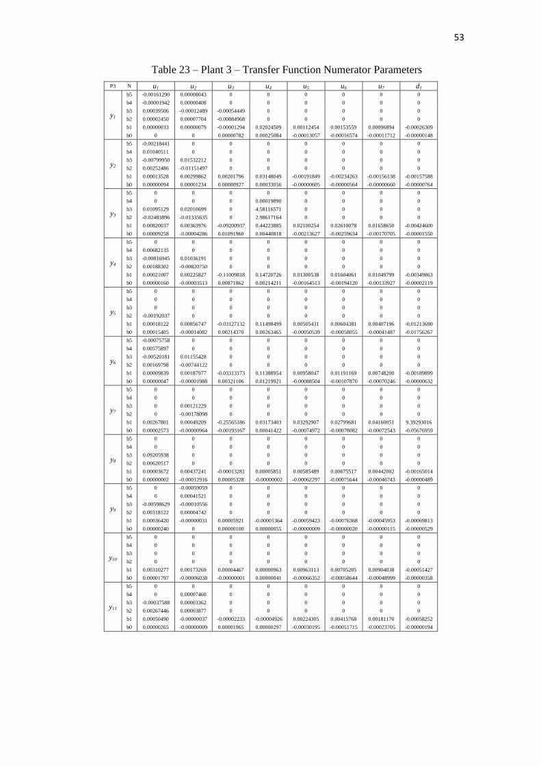
53

Table 23 – Plant 3 – Transfer Function Numerator Parameters

P3 N u1 u2 u3 u4 u5 u6 u7 d1

y1

b5 -0.00161290 0.00008043 0 0 0 0 0 0

b4 -0.00001942 0.00000408 0 0 0 0 0 0

b3 0.00039506 -0.00012489 -0.00054449 0 0 0 0 0

b2 0.00002450 0.00007704 -0.00884968 0 0 0 0 0

b1 0.00000033 0.00000079 -0.00001294 0.02024509 0.00112454 0.00153559 0.00096894 -0.00026309

b0 0 0 0.00000782 0.00025084 -0.00013057 -0.00016574 -0.00011712 -0.00000148

y2

b5 -0.00218441 0 0 0 0 0 0 0

b4 0.01040511 0 0 0 0 0 0 0

b3 -0.00799950 0.01532212 0 0 0 0 0 0

b2 0.00252486 -0.01151497 0 0 0 0 0 0

b1 0.00013528 0.00299862 0.00201796 0.03148049 -0.00191849 -0.00234263 -0.00156138 -0.00157588

b0 0.00000094 0.00001234 0.00000927 0.00033056 -0.00000605 -0.00000564 -0.00000660 -0.00000764

y3

b5 0 0 0 0 0 0 0 0

b4 0 0 0 0.00019890 0 0 0 0

b3 0.01095129 0.02010699 0 4.58116571 0 0 0 0

b2 -0.02483896 -0.01335635 0 2.98617164 0 0 0 0

b1 0.00820037 0.00363976 -0.09200937 0.44223885 0.02100254 0.02610078 0.01658650 -0.00424600

b0 0.00009258 -0.00004286 0.01091960 0.00440818 -0.00213627 -0.00259634 -0.00170705 -0.00001550

y4

b5 0 0 0 0 0 0 0 0

b4 0.00682135 0 0 0 0 0 0 0

b3 -0.00816945 0.01036191 0 0 0 0 0 0

b2 0.00188302 -0.00820750 0 0 0 0 0 0

b1 0.00021007 0.00225827 -0.11009818 0.14720726 0.01300538 0.01604061 0.01049799 -0.00349863

b0 0.00000160 -0.00003513 0.00871862 0.00214211 -0.00164513 -0.00194120 -0.00133927 -0.00002119

y5

b5 0 0 0 0 0 0 0 0

b4 0 0 0 0 0 0 0 0

b3 0 0 0 0 0 0 0 0

b2 -0.00192037 0 0 0 0 0 0 0

b1 0.00018122 0.00856747 -0.03127132 0.11498499 0.00505431 0.00604381 0.00407196 -0.01213690

b0 0.00015405 -0.00014082 0.00214370 0.00263465 -0.00050539 -0.00058055 -0.00041487 -0.01756267

y6

b5 -0.00075758 0 0 0 0 0 0 0

b4 0.00575897 0 0 0 0 0 0 0

b3 -0.00520181 0.01155428 0 0 0 0 0 0

b2 0.00169798 -0.00744122 0 0 0 0 0 0

b1 0.00009839 0.00187977 -0.03313173 0.11388954 0.00958047 0.01191169 0.00748200 -0.00189899

b0 0.00000047 -0.00001988 0.00321106 0.01219921 -0.00088504 -0.00107870 -0.00070246 -0.00000632

y7

b5 0 0 0 0 0 0 0 0

b4 0 0 0 0 0 0 0 0

b3 0 0.00121229 0 0 0 0 0 0

b2 0 -0.00178098 0 0 0 0 0 0

b1 0.00267801 0.00049209 -0.25565186 0.03173403 0.03292907 0.02799681 0.04160051 9.39293016

b0 0.00002573 -0.00000964 -0.00193167 0.00041422 -0.00074972 -0.00078082 -0.00072543 -0.05676959

y8

b5 0 0 0 0 0 0 0 0

b4 0 0 0 0 0 0 0 0

b3 0.09205938 0 0 0 0 0 0 0

b2 0.00620517 0 0 0 0 0 0 0

b1 0.00003672 0.00437241 -0.00013281 0.00005851 0.00585489 0.00675517 0.00442002 -0.00165014

b0 0.00000002 -0.00012916 0.00005328 -0.00000002 -0.00062297 -0.00075644 -0.00046743 -0.00000489

y9

b5 0 -0.00059059 0 0 0 0 0 0

b4 0 0.00041521 0 0 0 0 0 0

b3 -0.00598629 -0.00010556 0 0 0 0 0 0

b2 0.00318122 0.00004742 0 0 0 0 0 0

b1 0.00036420 -0.00000031 0.00005921 -0.00001364 -0.00059423 -0.00076368 -0.00045953 -0.00069813

b0 0.00000240 0 0.00000100 0.00000055 -0.00000009 -0.00000020 -0.00000115 -0.00000529

y10

b5 0 0 0 0 0 0 0 0

b4 0 0 0 0 0 0 0 0

b3 0 0 0 0 0 0 0 0

b2 0 0 0 0 0 0 0 0

b1 0.00310277 0.00173269 0.00004467 0.00000963 0.00963113 0.00705205 0.00904038 -0.00051427

b0 0.00001797 -0.00006038 -0.00000001 0.00000041 -0.00066352 -0.00058644 -0.00048999 -0.00000358

y11

b5 0 0 0 0 0 0 0 0

b4 0 0.00007460 0 0 0 0 0 0

b3 -0.00037588 0.00003362 0 0 0 0 0 0

b2 0.00267446 0.00003877 0 0 0 0 0 0

b1 0.00050490 -0.00000037 -0.00002233 -0.00004926 0.00224305 0.00415768 0.00181170 -0.00058252

b0 0.00000265 -0.00000009 0.00001965 0.00000297 -0.00030195 -0.00051715 -0.00023705 -0.00000194

54

Table 24 – Plant 3 – Transfer Function Denominator Parameters

P3 D u1 u2 u3 u4 u5 u6 u7 d1

y1

a5 1 1 0 0 0 0 0 0

a4 0.60616366 0.26006504 0 0 0 0 0 0

a3 0.04003953 0.04040114 1 0 0 0 0 0

a2 0.00083667 0.00285457 0.67672652 1 1 1 1 1

a1 0.00000422 0.00004973 0.02802616 0.34553608 0.39651350 0.41650526 0.43808977 0.01669236

a0 0 0.00000023 0.00019015 0.00290484 0.00327246 0.00341690 0.00367504 0.00004821

y2

a5 1 0 0 0 0 0 0 0

a4 0.73338773 0 0 0 0 0 0 0

a3 0.30252888 1 0 0 0 0 0 0

a2 0.03196168 0.13151790 1 1 1 1 1 1

a1 0.00055550 0.01411709 0.02875371 0.37612675 0.01499550 0.01383684 0.01664834 0.02144646

a0 0.00000227 0.00014080 0.00010432 0.00342748 0.00003450 0.00002557 0.00004824 0.00005771

y3

a5 0 0 0 0 0 0 0 0

a4 0 0 0 1 0 0 0 0

a3 1 1 0 30.57056552 0 0 0 0

a2 0.48323275 0.12222426 1 12.99983459 1 1 1 1

a1 0.02350459 0.01333325 1.15251139 1.24281174 0.34386181 0.34402516 0.33617157 0.02582544

a0 0.00015477 0.00024303 0.02663119 0.01061586 0.00711138 0.00704405 0.00710418 0.00006556

y4

a5 0 0 0 0 0 0 0 0

a4 1 0 0 0 0 0 0 0

a3 0.24682552 1 0 0 0 0 0 0

a2 0.02911368 0.10920344 1 1 1 1 1 1

a1 0.00052769 0.01078674 1.16076062 0.35068568 0.40412591 0.39464666 0.40185801 0.02103288

a0 0.00000218 0.00010262 0.01295549 0.00313854 0.00409003 0.00396640 0.00413259 0.00006688

y5

a5 0 0 0 0 0 0 0 0

a4 0 0 0 0 0 0 0 0

a3 1 0 0 0 0 0 0 0

a2 0.19728464 1 1 1 1 1 1 1

a1 0.03373426 0.04940690 0.37952403 0.46431275 0.17888196 0.17098216 0.17959950 9.65369794

a0 0.00021699 0.00033173 0.00289534 0.00343470 0.00123983 0.00117319 0.00126066 0.05530446

y6

a5 1 0 0 0 0 0 0 0

a4 0.65957664 0 0 0 0 0 0 0

a3 0.22269097 1 0 0 0 0 0 0

a2 0.02250019 0.13949382 1 1 1 1 1 1

a1 0.00051595 0.01467835 0.86032882 1.07844538 0.28219311 0.28348602 0.27530588 0.02936023

a0 0.00000196 0.00033151 0.02757344 0.06770926 0.00773520 0.00766312 0.00773408 0.00007096

y7

a5 0 0 0 0 0 0 0 0

a4 0 0 0 0 0 0 0 0

a3 0 1 0 0 0 0 0 0

a2 1 0.08725273 1 1 1 1 1 1

a1 0.03312328 0.01017913 0.73885014 0.33524447 0.94763699 0.75232933 1.26428402 276.11678502

a0 0.00018177 0.00012047 0.00858640 0.00288218 0.01360218 0.01074938 0.01827899 2.39957106

y8

a5 0 0 0 0 0 0 0 0

a4 0 0 0 0 0 0 0 0

a3 1 0 0 0 0 0 0 0

a2 0.01057821 1 1 1 1 1 1 1

a1 0.00004423 0.06299703 0.25806181 0.00496132 0.19510464 0.19640850 0.19460712 0.01029938

a0 0.00000001 0.00052878 0.00205527 0 0.00163304 0.00162326 0.00163627 0.00001868

y9

a5 0 1 0 0 0 0 0 0

a4 0 0.26640812 0 0 0 0 0 0

a3 1 0.04281507 0 0 0 0 0 0

a2 0.17198260 0.00341701 1 1 1 1 1 1

a1 0.00250734 0.00006023 0.05626396 0.07767206 0.00599493 0.00616802 0.00885345 0.02489282

a0 0.00000701 0.00000019 0.00025698 0.00041129 0 0.00000066 0.00001368 0.00006095

y10

a5 0 0 0 0 0 0 0 0

a4 0 0 0 0 0 0 0 0

a3 0 0 0 0 0 0 0 0

a2 1 1 1 1 1 1 1 1

a1 0.01741610 0.10980178 0.00917391 0.02118988 0.83101837 0.55217599 0.83145014 0.01907029

a0 0.00005770 0.00117154 0 0.00013578 0.00700103 0.00471769 0.00707324 0.00004898

y11

a5 0 1 0 0 0 0 0 0

a4 0 0.28079827 0 0 0 0 0 0

a3 1 0.04833173 0 0 0 0 0 0

a2 0.19768300 0.00445632 1 1 1 1 1 1

a1 0.00353637 0.00019380 0.54226850 0.13936678 0.33816196 0.46152256 0.34547457 0.01687142

a0 0.00001309 0.00000247 0.00646498 0.00174467 0.00440564 0.00595548 0.00453658 0.00003605

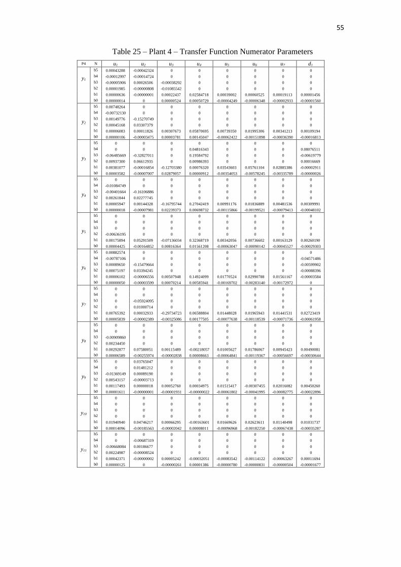
55

Table 25 – Plant 4 – Transfer Function Numerator Parameters

P4 N u1 u2 u3 u4 u5 u6 u7 d1

y1

b5 0.00043288 -0.00042324 0 0 0 0 0 0

b4 -0.00012997 -0.00014724 0 0 0 0 0 0

b3 -0.00005906 0.00026506 -0.00038292 0 0 0 0 0

b2 0.00001985 -0.00000808 -0.01085542 0 0 0 0 0

b1 0.00000636 -0.00000001 0.00022437 0.02584718 0.00039002 0.00060525 0.00019113 0.00001456

b0 0.00000014 0 0.00000524 0.00050729 -0.00004249 -0.00006348 -0.00002933 -0.00001560

y2

b5 0.00748264 0 0 0 0 0 0 0

b4 -0.00732130 0 0 0 0 0 0 0

b3 0.00149776 -0.15270749 0 0 0 0 0 0

b2 0.00045168 0.03307379 0 0 0 0 0 0

b1 0.00006083 0.00011826 0.00307673 0.05870695 0.00739350 0.01995306 0.00341213 0.00109194

b0 0.00000106 -0.00003475 0.00003781 0.00145047 -0.00062422 -0.00151898 -0.00036390 -0.00016813

y3

b5 0 0 0 0 0 0 0 0

b4 0 0 0 0.04816343 0 0 0 0.08076511

b3 -0.06485669 -0.32827011 0 0.19584792 0 0 0 -0.00619779

b2 0.00937300 0.06612935 0 0.00986393 0 0 0 0.00016669

b1 0.00381077 -0.00016854 -0.12703380 0.00076320 0.03543603 0.05761104 0.02885386 -0.00002911

b0 0.00003582 -0.00007007 0.02879057 0.00000912 -0.00354053 -0.00578245 -0.00335789 -0.00000026

y4

b5 0 0 0 0 0 0 0 0

b4 -0.01084749 0 0 0 0 0 0 0

b3 -0.00401664 -0.16106886 0 0 0 0 0 0

b2 0.00261844 0.02277745 0 0 0 0 0 0

b1 0.00005947 0.00144328 -0.16795744 0.27042419 0.00991176 0.01836889 0.00481536 0.00309991

b0 0.00000018 -0.00007981 0.02239373 0.00698732 -0.00115866 -0.00199521 -0.00079413 -0.00048102

y5

b5 0 0 0 0 0 0 0 0

b4 0 0 0 0 0 0 0 0

b3 0 0 0 0 0 0 0 0

b2 -0.00636195 0 0 0 0 0 0 0

b1 0.00175894 0.05291509 -0.07136034 0.32368719 0.00342056 0.00736602 0.00163129 0.00260190

b0 0.00004425 -0.00164852 0.00816364 0.01561208 -0.00063047 -0.00090142 -0.00045527 -0.00029303

y6

b5 0.00882574 0 0 0 0 0 0 0

b4 -0.00787106 0 0 0 0 0 0 -0.04571486

b3 0.00089650 -0.15479664 0 0 0 0 0 -0.00599902

b2 0.00075197 0.03394245 0 0 0 0 0 -0.00088396

b1 0.00006102 -0.00006556 0.00507948 0.14924099 0.01770524 0.02990788 0.01561167 -0.00003584

b0 0.00000050 -0.00003599 0.00070214 0.00585941 -0.00169702 -0.00283140 -0.00172972 0

y7

b5 0 0 0 0 0 0 0 0

b4 0 0 0 0 0 0 0 0

b3 0 -0.05924095 0 0 0 0 0 0

b2 0 0.01000714 0 0 0 0 0 0

b1 0.00765392 0.00032933 -0.29734723 0.06588804 0.01448028 0.01965943 0.01441531 0.02723419

b0 0.00005839 -0.00002389 -0.00325086 0.00177505 -0.00077638 -0.00118539 -0.00071736 -0.00061958

y8

b5 0 0 0 0 0 0 0 0

b4 0 0 0 0 0 0 0 0

b3 -0.00909860 0 0 0 0 0 0 0

b2 0.00234450 0 0 0 0 0 0 0

b1 0.00292877 0.07580051 0.00115489 -0.00218057 0.01005627 0.01786067 0.00945423 0.00490081

b0 0.00006589 -0.00255974 -0.00002838 0.00008663 -0.00064841 -0.00119367 -0.00056697 -0.00030644

y9

b5 0 0.03765047 0 0 0 0 0 0

b4 0 0.01481212 0 0 0 0 0 0

b3 -0.01369149 0.00089190 0 0 0 0 0 0

b2 0.00543157 -0.00003713 0 0 0 0 0 0

b1 0.00117493 0.00000018 0.00052760 0.00034975 0.01515417 -0.00307455 0.02016082 0.00450260

b0 0.00001611 -0.00000001 -0.00001931 -0.00000022 -0.00061802 -0.00041995 -0.00082775 -0.00022896

y10

b5 0 0 0 0 0 0 0 0

b4 0 0 0 0 0 0 0 0

b3 0 0 0 0 0 0 0 0

b2 0 0 0 0 0 0 0 0

b1 0.01940940 0.04746217 0.00066295 -0.00163601 0.01669626 0.02623611 0.01140498 0.01031737

b0 0.00014096 -0.00185563 -0.00002042 0.00008011 -0.00096968 -0.00182250 -0.00067438 -0.00035287

y11

b5 0 0 0 0 0 0 0 0

b4 0 -0.00687319 0 0 0 0 0 0

b3 -0.00668084 0.00186677 0 0 0 0 0 0

b2 0.00224987 -0.00008524 0 0 0 0 0 0

b1 0.00042371 -0.00000002 0.00005242 -0.00032051 -0.00083542 -0.00114122 -0.00063267 0.00011694

b0 0.00000125 0 -0.00000261 0.00001386 -0.00000780 -0.00000831 -0.00000504 -0.00001677

56

Table 26 – Plant 4 – Transfer Function Denominator Parameters

P4 D u1 u2 u3 u4 u5 u6 u7 d1

y1

a5 1 1 0 0 0 0 0 0

a4 0.23296424 0.07863813 0 0 0 0 0 0

a3 0.08208049 0.00430576 1 0 0 0 0 0

a2 0.00758918 0.00005046 0.73141937 1 1 1 1 1

a1 0.00027850 0.00000006 0.02366003 0.41143877 0.06512178 0.08150280 0.05821337 0.04183427

a0 0.00000193 0 0.00016993 0.00508471 0.00064549 0.00082135 0.00056422 0.00038562

y2

a5 1 0 0 0 0 0 0 0

a4 0.23708439 0 0 0 0 0 0 0

a3 0.06591165 1 0 0 0 0 0 0

a2 0.00480229 0.05239921 1 1 1 1 1 1

a1 0.00020995 0.00222654 0.03984005 1.27894468 0.10426372 0.20629258 0.08168182 0.05338634

a0 0.00000144 0.00001732 0.00098598 0.01041943 0.00109114 0.00224910 0.00083210 0.00051304

y3

a5 0 0 0 0 0 0 0 0

a4 0 0 0 1 0 0 0 1

a3 1 1 0 0.43818533 0 0 0 0.06735221

a2 0.09688217 0.05125249 1 0.02483772 1 1 1 0.00416706

a1 0.00555968 0.00273708 0.92474185 0.00141974 0.24707656 0.31464865 0.30851965 0.00010757

a0 0.00003700 0.00003040 0.05252992 0.00001331 0.00481350 0.00663588 0.00583065 0.00000058

y4

a5 0 0 0 0 0 0 0 0

a4 1 0 0 0 0 0 0 0

a3 0.11694337 1 0 0 0 0 0 0

a2 0.00578770 0.05029504 1 1 1 1 1 1

a1 0.00006439 0.00278323 1.22673630 0.50232417 0.10301513 0.14395772 0.09151188 0.07403663

a0 0.00000016 0.00002836 0.02585690 0.00679653 0.00125117 0.00182626 0.00108903 0.00085042

y5

a5 0 0 0 0 0 0 0 0

a4 0 0 0 0 0 0 0 0

a3 1 0 0 0 0 0 0 0

a2 0.10104154 1 1 1 1 1 1 1

a1 0.00379845 0.04898411 0.43152954 0.79996287 0.06432041 0.06504308 0.05700327 0.04468609

a0 0.00002731 0.00043381 0.00587453 0.00937255 0.00053787 0.00059174 0.00047837 0.00037514

y6

a5 1 0 0 0 0 0 0 0

a4 0.21972097 0 0 0 0 0 0 1

a3 0.06659150 1 0 0 0 0 0 0.05154411

a2 0.00442000 0.05491795 1 1 1 1 1 0.01303801

a1 0.00019950 0.00300581 0.08144899 0.73302066 0.24001571 0.30546798 0.32850680 0.00021094

a0 0.00000132 0.00003921 0.00422347 0.01847968 0.00588219 0.00835938 0.00771513 0

y7

a5 0 0 0 0 0 0 0 0

a4 0 0 0 0 0 0 0 0

a3 0 1 0 0 0 0 0 0

a2 1 0.05272244 1 1 1 1 1 1

a1 0.04281203 0.00313944 1.01082640 0.55796812 0.26007935 0.31059134 0.32064062 0.45341583

a0 0.00024024 0.00003952 0.02169965 0.00805290 0.00431904 0.00543513 0.00522737 0.00718090

y8

a5 0 0 0 0 0 0 0 0

a4 0 0 0 0 0 0 0 0

a3 1 0 0 0 0 0 0 0

a2 0.12351264 1 1 1 1 1 1 1

a1 0.00484536 0.05383596 0.02844148 0.06383918 0.04919364 0.08293772 0.05958454 0.04818289

a0 0.00003158 0.00045160 0.00035422 0.00041686 0.00041126 0.00068875 0.00048580 0.00037573

y9

a5 0 1 0 0 0 0 0 0

a4 0 0.03660570 0 0 0 0 0 0

a3 1 0.00286174 0 0 0 0 0 0

a2 0.10169929 0.00002187 1 1 1 1 1 1

a1 0.00410603 0.00000033 0.06022577 0.00394322 0.14853279 0.14177080 0.30637232 0.16425635

a0 0.00001749 0 0.00049377 0 0.00102863 0.00074390 0.00197746 0.00093493

y10

a5 0 0 0 0 0 0 0 0

a4 0 0 0 0 0 0 0 0

a3 0 0 0 0 0 0 0 0

a2 1 1 1 1 1 1 1 1

a1 0.03593174 0.08606306 0.03073281 0.12177017 0.19248980 0.29722990 0.18198729 0.14743131

a0 0.00015891 0.00097574 0.00057639 0.00097667 0.00208356 0.00329687 0.00192737 0.00151117

y11

a5 0 1 0 0 0 0 0 0

a4 0 0.25190654 0 0 0 0 0 0

a3 1 0.01188150 0 0 0 0 0 0

a2 0.09248629 0.00035869 1 1 1 1 1 1

a1 0.00401231 0.00000029 0.01313662 0.04725453 0.01729359 0.01863502 0.01702169 0.02135520

a0 0.00001712 0 0.00068071 0.00179233 0.00017796 0.00016128 0.00015325 0.00075203

57

Table 27 – Manipulated Variables Positive Uncertainty Parameters

Table 28 – Disturbance Positive Uncertainty Parameters

Table 29 – Manipulated Variables Positive Uncertainty Parameters

Table 30 – Disturbance Negative Uncertainty Parameters