Assessing New Quantitative

Imaging Biomarkers

Chaya Moskowitz, Ph.D.

Department of Epidemiology and Biostatistics

Memorial Sloan Kettering Cancer Center

With thanks to Todd Alonzo and Alicia Toledano

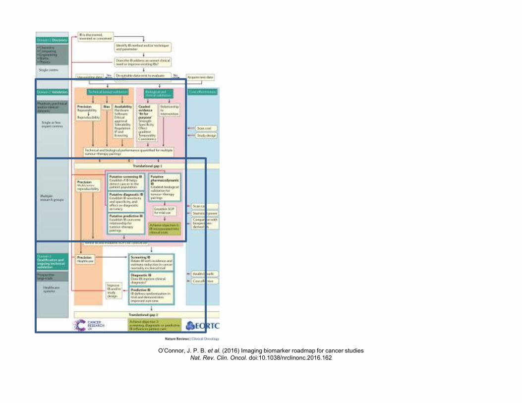
O’Connor, J. P. B. et al. (2016) Imaging biomarker roadmap for cancer studies

Nat. Rev. Clin. Oncol. doi:10.1038/nrclinonc.2016.162

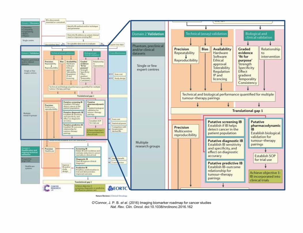
O’Connor, J. P. B. et al. (2016) Imaging biomarker roadmap for cancer studies

Nat. Rev. Clin. Oncol. doi:10.1038/nrclinonc.2016.162

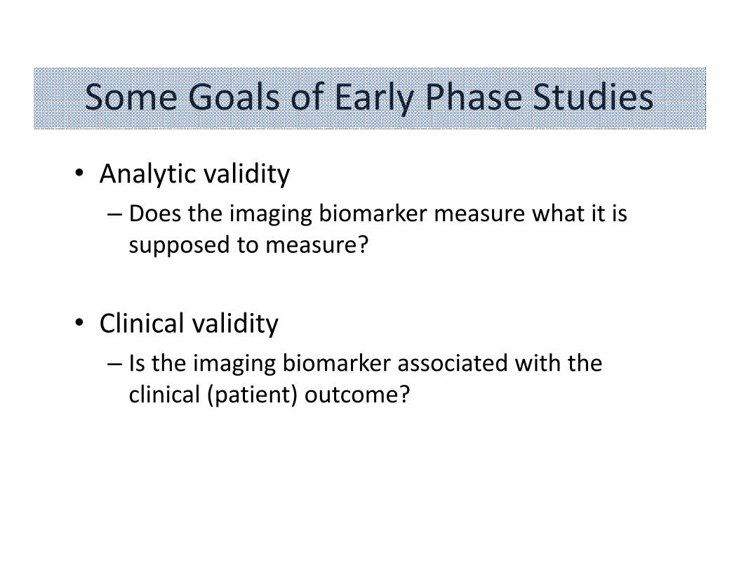
Some Goals of Early Phase Studies

• Analytic validity

– Does the imaging biomarker measure what it is

supposed to measure?

• Clinical validity

– Is the imaging biomarker associated with the

clinical (patient) outcome?

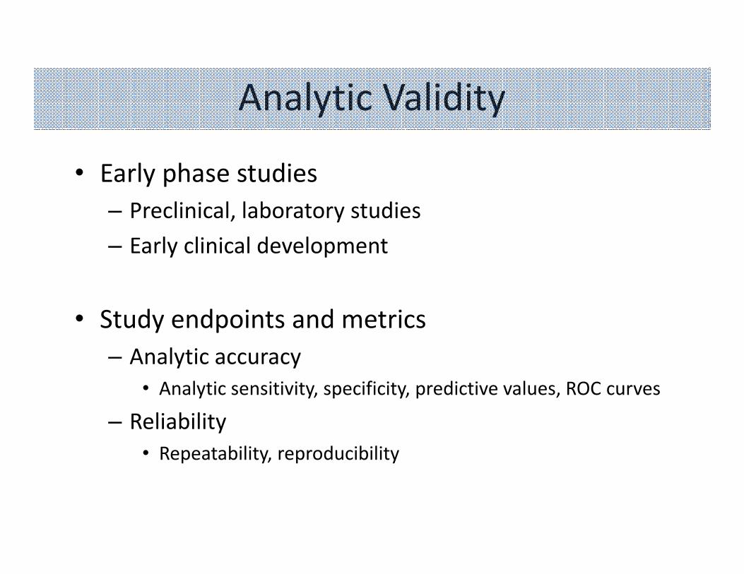
Analytic Validity

• Early phase studies

– Preclinical, laboratory studies

– Early clinical development

• Study endpoints and metrics

– Analytic accuracy

• Analytic sensitivity, specificity, predictive values, ROC curves

– Reliability

• Repeatability, reproducibility

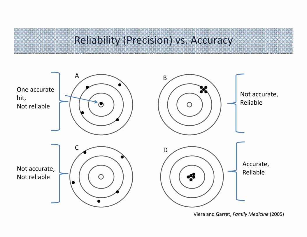
One accurate

hit,

Not reliable

A B

C D

Not accurate,

Reliable

Not accurate,

Not reliable

Accurate,

Reliable

Reliability (Precision) vs. Accuracy

Viera and Garret, Family Medicine (2005)

Importance

• Potential utility of an imaging biomarker can be greatly impacted by lack of reliability

• Poor reliability can make measured change in parameter difficult to interpret

• Developing reliable biomarkers can be difficult

• Acceptable magnitude depends on use– Strong agreement is a necessary component of any

subjective procedure intended for diagnostic use

Sources of Variability

• Patient-related

– Disease or treatment-related

– Other biophysiological sources

• Imaging system-related

– Scanner-related

– Reader-related

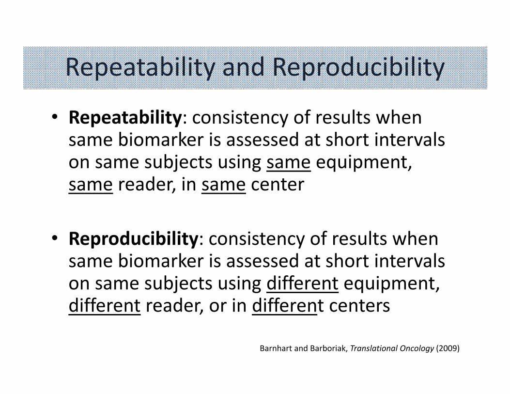
Repeatability and Reproducibility

• Repeatability: consistency of results when same biomarker is assessed at short intervals on same subjects using same equipment, same reader, in same center

• Reproducibility: consistency of results when same biomarker is assessed at short intervals on same subjects using different equipment, different reader, or in different centers

Barnhart and Barboriak, Translational Oncology (2009)

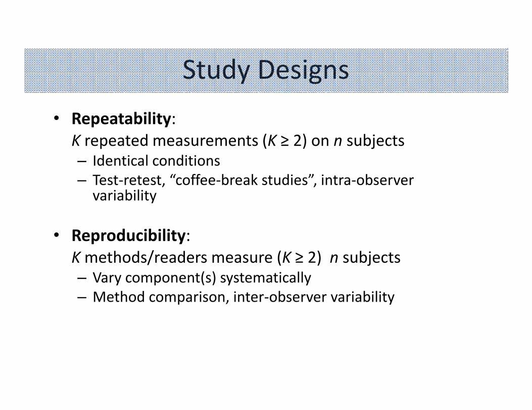
Study Designs

• Repeatability:

K repeated measurements (K ≥ 2) on n subjects

– Identical conditions

– Test-retest, “coffee-break studies”, intra-observer variability

• Reproducibility:

K methods/readers measure (K ≥ 2) n subjects

– Vary component(s) systematically

– Method comparison, inter-observer variability

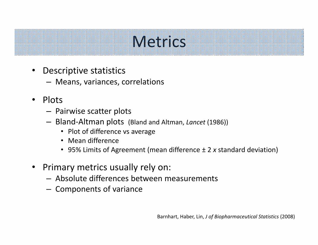
Metrics

• Descriptive statistics– Means, variances, correlations

• Plots– Pairwise scatter plots

– Bland-Altman plots (Bland and Altman, Lancet (1986))

• Plot of difference vs average

• Mean difference

• 95% Limits of Agreement (mean difference ± 2 x standard deviation)

• Primary metrics usually rely on:– Absolute differences between measurements

– Components of variance

Barnhart, Haber, Lin, J of Biopharmaceutical Statistics (2008)

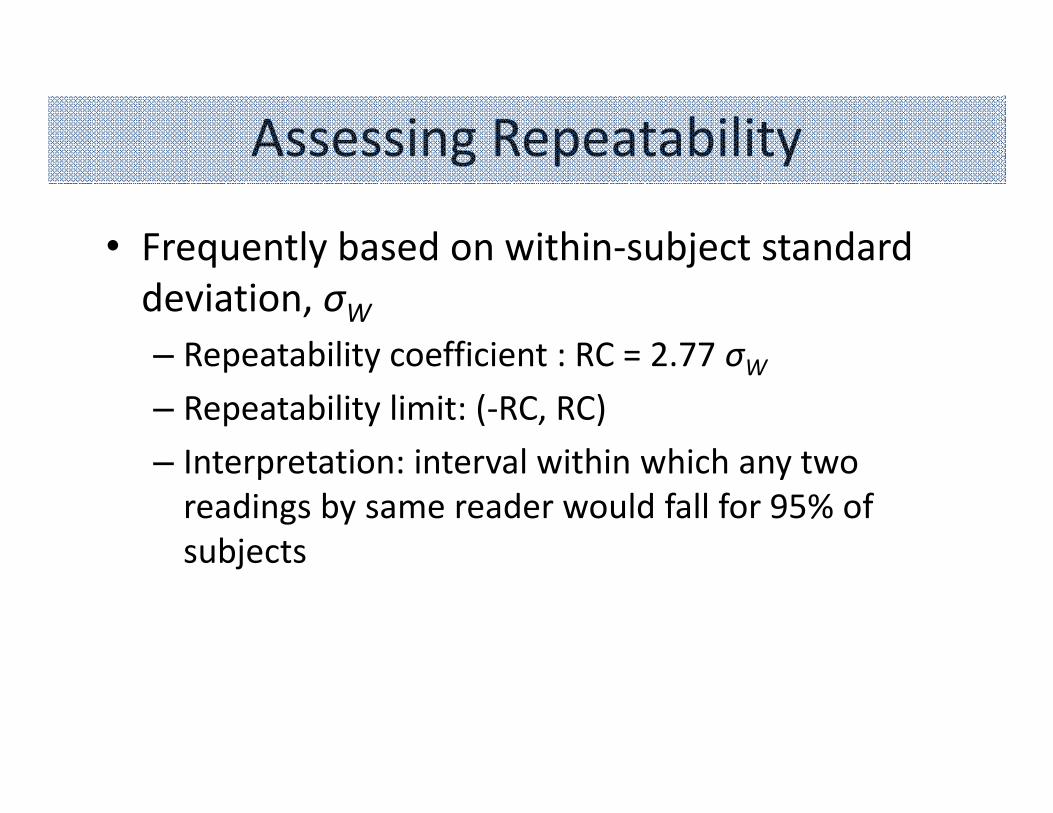
Assessing Repeatability

• Frequently based on within-subject standard

deviation, σW

– Repeatability coefficient : RC = 2.77 σW

– Repeatability limit: (-RC, RC)

– Interpretation: interval within which any two

readings by same reader would fall for 95% of

subjects

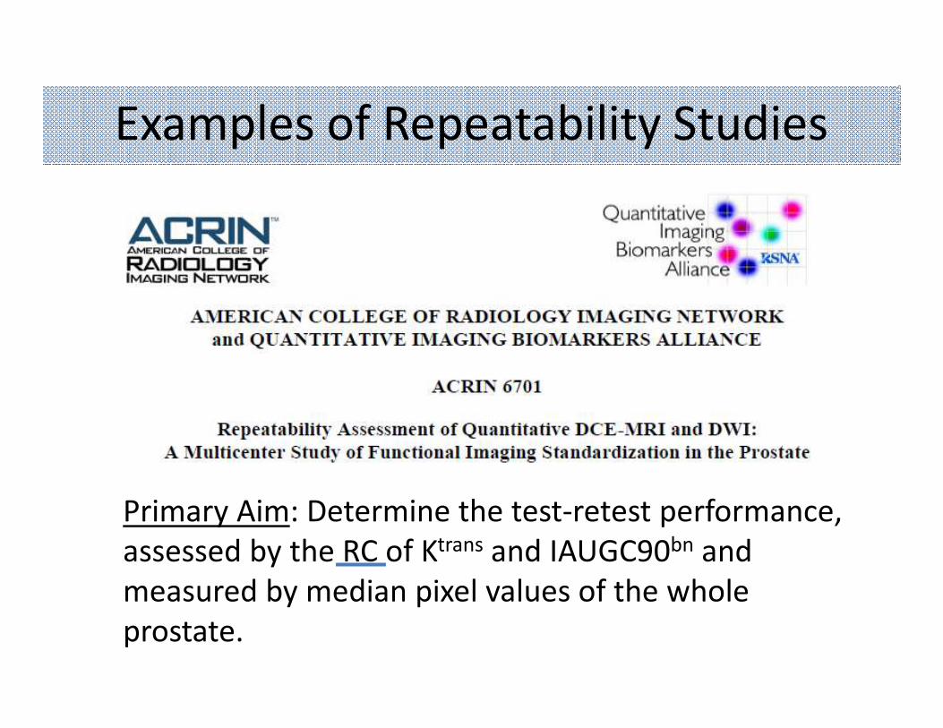
Examples of Repeatability Studies

Primary Aim: Determine the test-retest performance,

assessed by the RC of Ktrans and IAUGC90bn and

measured by median pixel values of the whole

prostate.

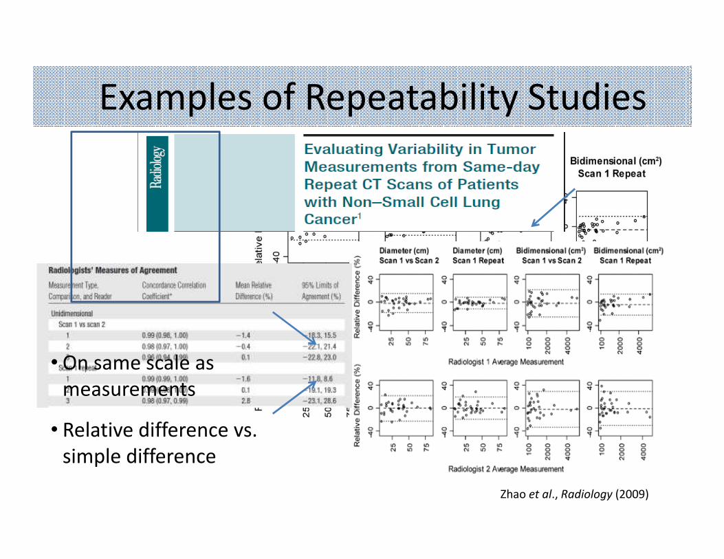
Examples of Repeatability Studies

Zhao et al., Radiology (2009)

• On same scale as

measurements

• Relative difference vs.

simple difference

Assessing Reproducibility

• Frequently based on between-subject standard deviation, σB

– Intraclass correlation coefficient

• ICC = σ2B /(σ2

B + σ2W)

• Interpretation: Proportion of total variance due to the different readers/methods

– Concordance correlation coefficient (Lin, Biometrics (1989))

• ρc = (2σX1X2)/(σ2

X1+ σ2

X2+ (µX1

- µX2)2)

• Interpretation: Quantifies agreement between two measurements

Examples of Reproducibility Studies

Kim et al., J of Magentic Resonance Imaging (2012)

Other Considerations

• Many other possible methods

• Continuous vs. categorical data– Contributes to choice of metrics

– Kappa statistics for categorical data

• Estimation rather than testing– P-values less interesting

– Confidence intervals

• Studies designed to evaluate both repeatability and reproducibility

Clinical Validity

• Mid-phase studies

– Clinical studies

– Retrospective and prospective

• Study endpoints and metrics

– Clinical sensitivity, specificity, predictive values, ROC curves

– Risk of the patient outcome for people with or without the imaging biomarker

Examples of Patient Outcomes

• Presence or absence of disease

• Tumor response rate

• Time to recurrence

• Progression free survival

• Disease free survival

• Overall survival

Survival Analysis

• Statistical methods for analyzing data where the outcome is the time to an event

• Applicable for data from single-arm clinical trials, randomized clinical trials, and cohort studies

• Important for: – Studies where not all patients enter at the same time

(staggered entry)

– Data analyzed before all patients have experienced the outcome (censoring)

Censoring

• Exact time event occurs is not known

• Different type of censoring:– Right censoring: event has not yet occurred

• Most common type of censoring

• Examples: study ends or patients are lost to follow-up

– Interval censoring: event occurred between two time-points, but we don’t know exactly when

• Examples: outcome occurs between two scheduled follow-up visits

– Left censoring: Event occurs before the study starts• Not usually found in clinical trials

Survival Data Example

Study

Start

Study

End

X

X

Calendar time Study

Start

Time on study

X

XX

X event censored

Definitions

• Primary interest:

T = the time until the event

• Instead observe:

C = the time at which an observation is censored

Y = min(T, C)

δ = 1 if the observation is censored, 0 otherwise

• Don’t throw away information on C!

• Record and give to your statistician: δ and Y– Example 1: Recurrence yes/no and time to recurrence or last follow-up

– Example 2: Recurrence yes/no and date of recurrence or last follow-up

Survival Function

• S(t) = Prob(T > t)

• Interpretation: Probability an individual experiences the event after time t; probability of surviving beyond time t.

• Starts at 1 and decreases towards 0:– S(t) =1 for t=0, S(t) = 0 for t=∞

• Nonincreasing function

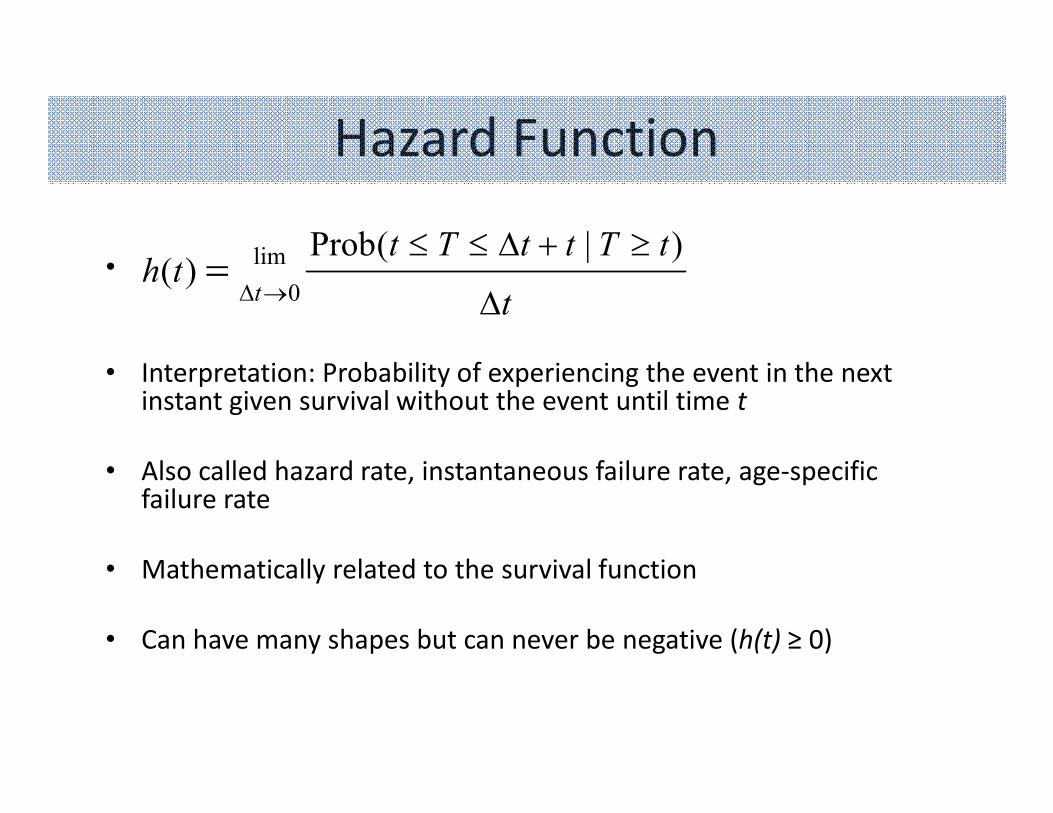
Hazard Function

•

• Interpretation: Probability of experiencing the event in the next instant given survival without the event until time t

• Also called hazard rate, instantaneous failure rate, age-specific failure rate

• Mathematically related to the survival function

• Can have many shapes but can never be negative (h(t) ≥ 0)

t

tTttTtth

t ∆

≥+∆≤≤→∆

=)|(Prob

)(0

lim

Estimating the Survival Function

• To estimate S(t) = Prob(T>t), why not just take the proportion of people with event times greater than t?– Ignores censoring

• Two main ways:– Parametric estimate

• Assumes the times-to-event follow a particular probability distribution function

– Non-parametric estimate• Empirical estimate

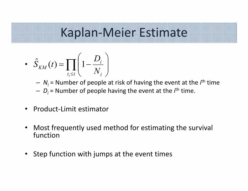
Kaplan-Meier Estimate

•

– Ni = Number of people at risk of having the event at the ith time

– Di = Number of people having the event at the ith time.

• Product-Limit estimator

• Most frequently used method for estimating the survival function

• Step function with jumps at the event times

∏≤

−=

tt i

iKM

iN

DtS 1)(ˆ

0.0

00

.25

0.5

00

.75

1.0

0

0 5 10 15 20analysis time

Kaplan-Meier survival estimate

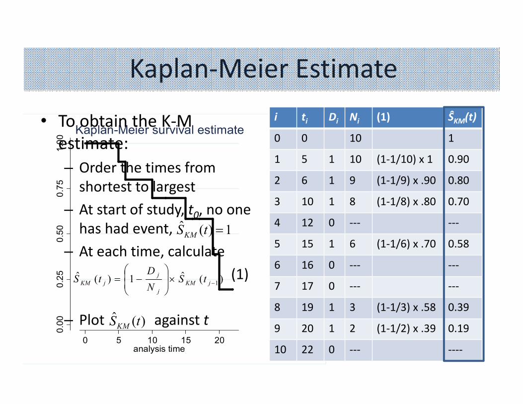
Kaplan-Meier Estimate

• To obtain the K-M

estimate:

– Order the times from

shortest to largest

– At start of study, t0, no one

has had event,

– At each time, calculate

(1)

– Plot against t

i ti Di Ni (1) ŜKM(t)

0 0 10 1

1 5 1 10 (1-1/10) x 1 0.90

2 6 1 9 (1-1/9) x .90 0.80

3 10 1 8 (1-1/8) x .80 0.70

4 12 0 --- ---

5 15 1 6 (1-1/6) x .70 0.58

6 16 0 --- ---

7 17 0 --- ---

8 19 1 3 (1-1/3) x .58 0.39

9 20 1 2 (1-1/2) x .39 0.19

10 22 0 --- ----

1)(ˆ =tSKM

)(ˆ1)(ˆ1−×

−= jKM

j

j

jKM tSN

DtS

)(ˆ tSKM

Caveats

• Assume probability an observation is censored is unrelated to the probability of having an event– Uninformative censoring

• Estimates can be unstable at the tail of the Kaplan-Meier curve when the number of patients remaining at risk gets small

• If the last observation is censored the Kaplan-Meier estimate will not reach 0.

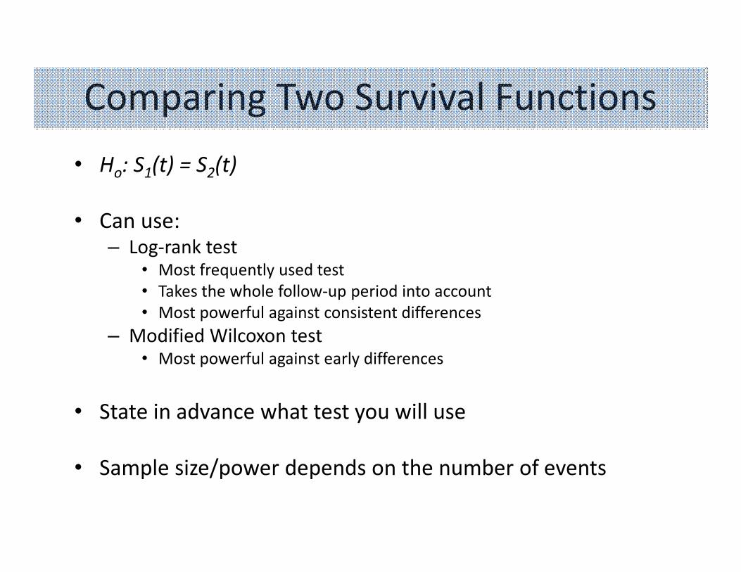
Comparing Two Survival Functions

• Ho: S1(t) = S2(t)

• Can use:– Log-rank test

• Most frequently used test

• Takes the whole follow-up period into account

• Most powerful against consistent differences

– Modified Wilcoxon test• Most powerful against early differences

• State in advance what test you will use

• Sample size/power depends on the number of events

Time-Dependent ROC Curves

• Disease status changes over time

• ROC curves that change as a function of time

• Can define based on the survival function

Heagerty et al. Biometrics 2000

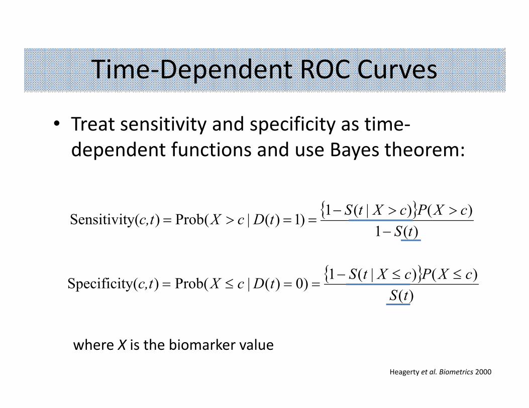
• Treat sensitivity and specificity as time-

dependent functions and use Bayes theorem:

Time-Dependent ROC Curves

{ })(1

)()|(1)1)(|(Prob)y(Sensitivit

tS

cXPcXtStDcXc,t

−>>−

==>=

{ })(

)()|(1)0)(|(Prob)y(Specificit

tS

cXPcXtStDcXc,t

≤≤−==≤=

where X is the biomarker value

Heagerty et al. Biometrics 2000

• Retrospective study

• Used archived echocardiograph images on 416 patients with chronic systolic heart failure

• Speckle-tracking analysis of left ventricular longitudinal, circumferential, and radial strain and strain rate

• Outcome: prognosis as defined by all-cause mortality, cardiac transplantation, or ventricular assist device placement

• Short- and long-term prognosis

Time-Dependent ROC Curves:Example using Strain in Chronic Heart Failure

Time-Dependent ROC Curves:Example using Strain in Chronic Heart Failure

(t = 1 year) (t = 5 years)

Zhang et al. J Am Heart Assoc. 2013

Summary

• Critical to assess analytic validity; many studies do not rigorously assess analytic validity

• Consistency of results when biomarker assessed at short intervals on same subjects– Using same equipment in same center (Repeatability )

– Using different equipment in different centers (Reproducibility)

• With time-to-event data, important to properly account for unobserved events

35