Assessing Individual Risk attitudes Using

Field Data from Lottery Games* Connel Fullenkamp Rafael Tenorio Duke University DePaul University

and

Robert Battalio University of Notre Dame

* We thank Gabriella Bucci, Larry Samuelson, Richard Sheehan, various workshop participants, and two anonymous referees for numerous comments. Part of this project was completed while Tenorio visited the Management and Strategy Department at Northwestern University. He is thankful for their hospitality. Trish and Marcos Delgado provided superb research assistance. All errors or omissions are the authors'. Please address correspondence to: Rafael Tenorio, DePaul University, Department of Economics, 1 E. Jackson Blvd. – Suite 6200, Chicago, IL 60604-2287. E-mail: rtenorio@condor.depaul.edu.

Assessing Individual Risk attitudes Using Field Data from Lottery Games

Abstract We use information from the television game show with the highest guaranteed average payoff in the U.S.,

Hoosier Millionaire, to analyze risk-taking in a high-stakes experiment. We characterize gambling

decisions under alternative assumptions about contestant behavior and preferences, and derive testable

restrictions on individual risk attitudes based on this characterization. We then use an extensive sample of

gambling decisions to estimate distributions of risk aversion parameters consistent with the theoretical

restrictions and revealed preferences. We find that although most contestants display risk averse

preferences, the extent of the risk aversion implied by our estimates varies substantially with the stakes

involved in the different decisions.

JEL Codes: C93, D81, C15

1

I. Introduction

A series of recent studies (Rabin 2000a, 2000b; Rabin and Thaler 2001) have pointed out the inadequacy of

expected utility theory to provide proper characterization of risk aversion when monetary stakes are small.

The basic contention of this criticism is that the concavity of the utility function would have to be so

pronounced to explain small stake risk aversion, that this same utility function would imply absurd levels of

risk aversion for large stakes. Rabin (2000b) concludes that "Expected-utility theory seems to be a useful

and adequate model of risk aversion for many purposes, such as understanding large-stakes insurance…,"

but "is manifestly not close to the right explanation of risk attitudes over modest stakes…"

A number of studies have attempted to characterize individual risk aversion under relatively large

stakes using expected utility theory. Experiments by Binswanger (1981), and Kachelmeier and Shehata

(1992) face subjects with decisions involving small nominal stakes that are large relative to the subjects'

wealth. Their findings are mixed: while the Binswanger subjects exhibit more risk averse behavior as

stakes are increased, Kachelmeier and Shehata conclude that "the effects of monetary payoffs are real, albeit

subtle, and are in need of further study." Unfortunately, the inherent limitations of rewards in experimental

studies make it difficult to get more robust conclusions about risk-taking in large stakes settings.

A second group of papers analyzes risk-taking behavior using information from natural experiments

involving large stakes. Gertner (1993) uses betting decisions from the bonus round of the television game

show Card Sharks, and concludes that individuals exhibit a small degree of risk aversion. Metrick (1995),

Hersch and McDougall (1997), analyze field data from wagering decisions on the television game shows

Final Jeopardy! and Illinois Instant Riches, respectively, and find that contestants display behavior that is

statistically indistinguishable from risk neutrality. In contrast, Beetsma and Schotman (1999), conclude that

contestants in the Dutch television show LINGO, exhibit substantial risk aversion.

In this paper we use information from the television show Hoosier Millionaire to gain additional

insight into the behavior of individuals in high stakes situations. Although this show has undergone a

number of regime changes, the current regime is representative of the typical decision a contestant faces:

she may either (a) take a sure $100,000, or (b) play a game in which she gets $150,000, $200,000,

2

1,000,000, or $0, each with equal probability. If she draws $150,000 or $200,000, she may stop playing and

keep the prize, or continue drawing from the remaining alternatives until she either decides to stop, or draws

$0 or $1,000,000. Prizes are not cumulative.

We believe, for various reasons, that the structure of the decision problems in Hoosier Millionaire

provides us with a very appealing natural experiment to study individual decisions under risk. First, unlike

previous game studies, the realization of the risky prospect is the outcome of a very simple probability

process, where no subjectivity or skills are involved 1. Second, the stakes are larger than those in previous

studies, thus allowing a more proper characterization of risk aversion using expected utility theory. Finally,

our data comprises a time series of games involving several regime changes, which allows us to study the

sensitivity of individual behavior across various gambles.

Our approach to analyzing risk aversion differs significantly from previous game-based studies.

Exogenous wagers and lack of variation in the gambles prevent us from estimating risk aversion parameters

using regression techniques. Instead, we use the sample properties of the decisions in the different regimes

of Hoosier Millionaire to estimate the parameters of the distribution of risk aversion coefficients in the

contestant population. In addition, unlike previous studies, we explicitly account for various degrees of

contestant rationality in our estimation.

Our results show that most individuals behave in a way consistent with risk aversion, and as noted in

recent studies, the implied degree of risk aversion varies largely with the stakes of the decision. In fact, our

estimates imply substantial risk aversion for gambles comparable to those in Hoosier Millionaire, while also

implying near risk neutrality for smaller gambles of similar structure. We also show that the impact of

different behavioral traits on decisions and risk aversion is only evident under large stakes.

II. A Brief History of Hoosier Millionaire

The Hoosier Lottery’s weekly television show, Hoosier Millionaire, first aired on October 28, 1989.

Since its inception, each show has involved six contestants chosen randomly from a pool of entries

submitted by people playing a scratch-off ticket game. All contestants participate in the first of two

phases played on each show. In Phase I, all six contestants play a series of purely random draw games.

3

The contestant who amasses the most cash wins and proceeds to Phase II, while the remaining five

contestants leave the show. All six contestants keep the cash and prizes accumulated in Phase I.

Four regimes have governed Phase II of Hoosier Millionaire. In Regime 1, the Phase I winner has

the option of choosing one of four numbers randomly associated with the dollar amounts $50,000,

$100,000, and $1,000,000, and a consolation prize of $25,000. If the contestant draws $1 million, she wins

that amount, paid-out in 10 equal annual payments, and the game is over. If the contestant draws $50,000 or

$100,000, she can keep that amount or give it up and make another choice among the remaining

alternatives. She continues until she chooses to stop, wins the $1 million, or draws the consolation prize.

In October of 1990, the two intermediate amounts offered in the gamble changed from $50,000 and

$100,000 to $100,000 and $200,000. All other features remained the same. We call this Regime 2.

In February of 1992, more changes were made to Phase II. First, the lowest amount attainable in the

initial drawing changed from $100,000 to $150,000. Second, the consolation prize went down from

$25,000 to 1,000 scratch-off lottery tickets with a purchase price of $1 each. Finally, lottery officials

changed the payment of the $1 million prize to twenty annual payments of $50,000. We call this Regime 3.

Rules currently governing Phase II of Hoosier Millionaire were instituted in February of 1994.

According to Pat Traub, the lottery's acting deputy director, these changes offer "...the highest guaranteed

prize of any game show in the nation..." and were made to "...enhance the show's entertainment value."

Two revisions were made. First, a contestant is now automatically endowed with a guaranteed $100,000

prize. She may then decide to keep that amount and walk away from the show, or give it up and choose

one of the four numbers just as in Regime 3. The other change involved extending the period of time

over which the $1,000,000 prize is paid out from twenty to twenty-five years 2. We call this Regime 4.

III. Analytical Issues

In analytical terms, the problem a Hoosier Millionaire contestant faces is one of sequential decisions with

no recall. This means that the outcome of the first decision may give the contestant the option to continue

playing, but once a continuation decision is made at any stage, the status quo is no longer available. In a

problem like this, the optimal decisions follow from using a dynamic programming (or backward induction)

4

technique. This means starting at the final decision node, assessing the values of continuing and stopping at

that stage, and then factoring in these values when making decisions at the previous stage(s). This procedure

is equivalent to finding the subgame perfect equilibrium in a game against nature.

In analyzing the optimal strategy for each regime, we consider the following behavioral hypotheses:

Full Rationality (FR). A contestant performs backward induction at each decision node, and discounts the

$1,000,000 prize based on the annuity system 3.

Bounded Rationality 1 (BR1). Same as FR but no discounting is applied to the $1,000,000 prize.

Bounded Rationality 2 (BR2). Contestants do not perform backward induction at every decision node, i.e.,

they do not take into account the value of the option to continue playing the game, and evaluate each lottery

as a simple rather than a sequentially compounded lottery. Annuities are discounted.

Bounded Rationality 3 (BR3). Same as BR2 but annuities are not discounted.

Our bounded rationality scenarios are motivated by biases observed in decision settings comparable

to our problem. Empirical and experimental evidence suggests that low or even negative discounting is

common in decisions involving evaluation of income streams over time (BR1, BR3). Loewenstein and

Prelec (1991), Loewenstein and Thaler (1989), and Gigliotti and Sopher (1997), note that most subjects

prefer a more constant and spread out stream of income over a strictly decreasing pattern of payments 4, 5.

There is also extensive evidence that individuals fail to perform backward induction in sequential

decision environments (BR2, BR3). Carbone and Hey (1998), report a series of decision-making

experiments where individuals do not apply Bellman’s Principle of Optimality. Similarly, Camer et. al.

(1993) show that subjects do not reason backwards in simple alternating-offers bargaining experiments.

Instead, most subjects base their decision on current round payoffs 6.

Figures 1 and 2 show the game trees associated with Regimes 3 and 4 of Hoosier Millionaire. We

subsequently analyze optimal decisions under each of the behavioral hypotheses outlined above.

(i) Risk neutrality.

If decisions depend solely on expected values at each decision node, simple calculations show that:

5

(a) Boundedly rational contestants who do not discount annuities (BR2 and BR4) always choose the gamble

over the sure prospect. Here, the $1,000,000 prize makes the gambles’ expected values very large across the

board, even when contestants do not backward induct.

(b) If contestants discount annuities (FR and BR2), gambling may become unattractive as discounting

increases. Table 1 shows the discount rates that make a contestant indifferent between gambling and

keeping the sure prospect at the various decision nodes. As shown, for sufficiently low discount rates

(r<10.014%), it is optimal to gamble in any regime at any decision node for both the FR and BR2 contestant

types. As discounting increases, some of the gambles' expected values fall below the sure prospects. In

Regimes 1 and 2, discount rates must be very high (above 22%) to discourage individuals from gambling.

This is because the $1 million annuity payments are only spread across 10 years and the consolation prize is

substantial ($25,000). In Regimes 3 and 4, where annuities are paid over 20-25 years and the consolation

prize is only $1,000, lower discount rates may induce individuals to take on various gambles.

(ii) Risk Aversion 7.

To make our results comparable to those of previous studies we assume that Hoosier Millionaire

contestants display one of the following two types of preferences:

Constant Absolute Risk aversion (CARA). These preferences, which imply increasing relative risk

aversion, are often assumed in studies of individual decision-making. Their generic utility representation is:

aWeWU −−=)( (1),

where W is the individual's wealth, a is the coefficient of absolute risk aversion, and aW is the coefficient of

relative risk aversion. This formulation is convenient because it allows one to calculate absolute risk

aversion coefficients without any wealth information.

Constant Relative Risk aversion (CRRA). These preferences, which imply decreasing absolute risk

aversion, are commonly used in macro and asset-pricing studies. Their generic utility representation is:

b

WWUb

−=

−

1)(

)1(

(2),

6

where W is the individual's wealth, b is the coefficient of relative risk aversion, and b/W is the coefficient of

absolute risk aversion. Since this formulation implies that risk aversion depends on wealth, we must know

something about this variable to make meaningful inferences. Given lack of comprehensive wealth

information, we make alternative assumptions about the reference wealth level that individuals use to make

decisions. We first use a restrictive definition of wealth, W0, encompassing only the winnings accumulated

in Hoosier Millionaire. This partial asset integration in decision-making is to some extent consistent with

Kahneman and Tversky's Prospect Theory. As a test of robustness we will also use a broader wealth

definition (W1), which includes the median household income of the individual’s Census Tract in 1990.

Table 2 shows the values for the CARA and CRRA (W0) parameters that make contestants indifferent

between gambling and keeping the sure prospect on every initial subgame in every regime of Hoosier

Millionaire. That is, for any risk aversion parameter larger than a given parameter in this table, the

contestant will prefer the sure prospect to the gamble.

As expected, as discounting increases, the value of the $1,000,000 annuity payments becomes small

relative to the lump-sum payoffs. Thus, at some discount rate the expected value of a gamble becomes

smaller than the sure prospect, and the contestant would have to be a risk lover to gamble (see selected

entries in Table 2 when r=20% and r=30%). Also, for a given discount rate, the risk aversion coefficient

that dissuades a contestant from gambling decreases with the amount of the sure prospect, regardless of the

degree of contestant rationality. This follows from certainty-equivalence.

IV. Data

We obtained the Hoosier Millionaire data from the Hoosier Lottery office in Indianapolis, and from press

releases in the South Bend Tribune. With a few exceptions, our data set contains the winnings and Census

Tract characteristics of all the participants in both phases of Hoosier Millionaire since its original inception.

Table 3 presents a summary of the contestants' endogenous initial gambling decisions 8. We also

report mean Phase 1 winnings and 1990 Census Tract median income figures for our sample. As seen in

Table 3, although 58% of the individuals in our sample take the initial gamble, this fraction varies across

regimes. In fact, the rough comparative statics of decisions across regimes indicate that contestants

7

correctly respond to changes in the award structure. For instance, in Regime 1 the sizable consolation prize

($25,000) substantially reduces the downside of gambling. As a result, all of the contestants in this regime

choose to gamble. This contrasts with Regime 3, where the small consolation prize ($1,000) makes the

downside of gambling rather onerous, thus inducing 40 of 45 contestants to keep the sure prospect.

The fourth column of Table 3 shows Phase 1 winnings for each contestant in our data set. As seen,

there is not much variation in these winnings. We obtained the addresses of all Phase 2 Hoosier Millionaire

contestants, and found matching data from their 1990 Census Tracts. Table 3 also shows the average

median family and per-capita income for our sample. Although both of these income measures are below

state averages, they are not significantly different from them 9. However, there is no systematic difference

between the incomes of contestants that took the gambles and contestants that chose the certain prospects 10.

V. Estimation

(i) Methodology

Previous studies such as Gertner (1993), Metrick (1995), and Hersch and McDougall (1997) estimated the

coefficient of absolute risk aversion using a non-linear probit approach. Unlike those studies, where

individuals face gambles involving different stakes, each contestant within a regime of Hoosier Millionaire

faces a gamble with identical stakes. Thus the probit technique is inappropriate because a key source of

variation --that between the size of each gamble-- is absent.

Instead, we use a probabilistic approach and estimate the distribution of the risk aversion parameter.

We assume that contestants are endowed with risk aversion parameters that are independent draws from a

normal population distribution 11. If a contestant's realization of the risk aversion parameter is less than the

value that yields indifference, or equality of expected utilities from gambling and not gambling, she chooses

the gamble. The probability that the contestant's risk aversion parameter lies below the indifference value is

given by the value of the cumulative normal distribution evaluated at the indifference value.

As we know, the normal distribution depends on its mean and standard deviation. To estimate these

parameters, we use the indifference values in Table 2 and the binomial probabilities implied by the

empirical frequencies in Table 3. We infer the mean and standard deviation as follows: Each subgame in

8

the history of Hoosier Millionaire is associated with a CARA or CRRA indifference parameter, which we

denote ρ, and an observed frequency of taking the gamble, denoted p. We choose pairs of subgames, and

solve for the (unique) values of the mean µ and standard deviation σ that satisfy the following system:

12

)(

21

21

2

2

)2( pdxex

=∫∞−

−−−ρσ

µ

σπ (3a)

22

)(

21

22

2

2

)2( pdxex

=∫∞−

−−−ρσ

µ

σπ (3b)

We then used Monte Carlo simulations to place confidence intervals around the estimated mean and

standard deviation. For each Monte Carlo trial, we generated two data sets consisting of indicator random

variables, and used the implied p’s from this pseudo data to solve for µ and σ. The data generating process

for each set of indicator variables was a binomial distribution with parameter (probability of success on each

binomial trial) equal to the observed p from the respective subgame. The number of observations in each set

of pseudo data was set equal to the number of actual observations of the respective subgame. We repeated

this experiment 1,000 times for each regime pair and behavioral assumption, ranked the estimated means

and standard deviations, and identified 90% confidence intervals.

Although we performed this experiment using several pairs of subgames, we focus on the pairing of

Regimes 4 and 3.2. 12. Table 4 reports estimated means and variances of the CARA and CRRA coefficients

for each behavioral assumption, along with the Monte Carlo generated 90% confidence intervals.

(ii) Results

A feature of our results is their robustness across utility specifications. The parameter estimates for the

CARA and CRRA(Wo) functions yield similar distributions and exhibit comparable patterns. The following

discussion makes use of this similarity by grouping the results from both specifications whenever possible.

First, our results consistently support risk aversion. Estimated mean risk aversion coefficients are

always positive and the confidence intervals around these means never include zero. Mean risk aversion

parameter estimates under CARA range from 4.8E-6 to 9.7E-6, while those under CRRA utility range from

0.64 to 1.43. Moreover, the minimum means implied by the Monte Carlo simulations are always positive.

9

This evidence supports the hypothesis that on average, the individuals on our sample are risk averse.

However, the estimated standard deviations of the risk aversion parameters indicate that some individuals

may display risk neutral or risk loving preferences. This is particularly the case for CRRA utility, where a

significant fraction of estimated risk aversion parameters are non-positive. A two-standard deviation

interval around the mean risk aversion parameter generally includes only positive values for the CARA

utility function but encompasses zero and negative values in the CRRA case.

Our second main result is that different behavioral assumptions affect the estimates of mean risk

aversion. For fixed discounting, confidence intervals for these means under full rationality (FR) and non-

backward induction (BR2 and BR3) are mutually exclusive. In addition, when comparing no discounting

and 10% discounting, holding behavior fixed, confidence intervals are mutually exclusive in three of four

cases. We discuss the direction and significance of these differences in the next section.

As a test of robustness of our CRRA results, we estimated the distribution parameters using a more

inclusive definition of wealth (W1). In this specification, in addition to Phase I winnings, the initial wealth

also included the average median income for the contestant’s Census Tract in 1990. As we see in Table 4,

the higher initial wealth uniformly increases the means and standard deviations of the CRRA parameter

distributions. However, most of these increases are of very small order (between 0.1 and 0.3), and as we

show in the next section, do not affect the basic interpretation of the results. The similarity between the two

sets of CRRA estimates is due to the fact that that both wealth definitions are a relatively small fraction of

the stakes of the gambles in Hoosier Millionaire 13.

VI. Discussion and Conclusions

The results from the previous section uniformly indicate that most individuals display some degree of risk

aversion. To gain insight into the economic significance of these results, we first compare them to those

obtained in related work. Our estimated means of the CARA parameter distributions are lower than the

estimated CARA parameters of other game show studies. Gertner (1993), using two alternative methods,

estimates statistically significant lower bounds on this parameter of 0.000310 or 0.0000711. Metrick (1995),

and Hersch and McDougall (1997) report estimates ranging from 0.0000265 to 0.000066, but these

10

estimates are not statistically different from zero, leading to the conclusion of risk neutrality. In contrast,

our largest estimated mean CARA parameter is 0.0000097, and the largest upper bound on a confidence

interval is 0.000012, both of which are nearly an order of magnitude smaller than those reported elsewhere.

Our CRRA parameter estimates are also generally lower than those reported elsewhere. Friend and

Blume (1975), using data from individual portfolio holdings find estimates of this parameter ranging from 1

to 2, while Chou et. al. (1992), in an asset-pricing context, estimate this parameter to be around 3. Beetsma

and Schotman (1999), using game data from LINGO, estimate this parameter to be around 7. In our case the

mean CRRA parameters range from 0.64 to 1.76, once again below most estimates from other studies.

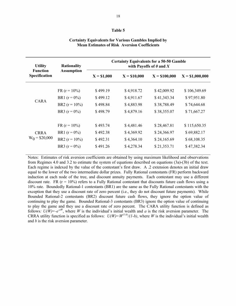
To gain some intuition into the meaning of our results and how they compare to those of other

studies, we calculate certainty equivalents implied by our mean estimates for a variety of gambles (see Table

5). For instance, for a gamble offering a 50-50 chance of winning nothing and $1,000, the certainty

equivalent ranges from $461.40 (Gertner 1993) to $496.73 (Hersch and McDougall 1997), with most

estimates implying a certainty equivalent above $490. In our experiments, certainty equivalents implied

by point estimates of the mean of the parameter distribution range from $491.26 to $499.40. Thus for

gambles of this magnitude, not only are our results similar to those in other studies, but they imply

behavior close to risk neutrality. Moreover, the tightness of the range of these certainty equivalents

indicates that the differences among risk aversion parameters across behavioral assumptions may not have

much economic significance when stakes like these are involved. In fact, as seen in Table 5, near risk

neutrality across all behaviors obtains even as stakes rise to several thousand dollars. This point, also

emphasized on Table 1 of Rabin and Thaler (2001), suggests that gambles of this size unavoidably lead to

parameter estimates that imply near risk neutrality within the expected utility paradigm. Thus, given that

most previous studies based their estimates on gambles with maximum stakes around $20,000, it is not

surprising at all that the results point towards risk neutrality or mild risk aversion 14.

However, we estimated our risk aversion parameters from decisions involving unusually high stakes.

In fact, stakes in Hoosier Millionaire are several orders of magnitude (20 or more in most cases) higher than

those in any of the games analyzed in other studies. Thus, we must base our inferences on stakes of this

11

magnitude. For instance, for a 50-50 gamble between winning nothing and $1 million, the certainty

equivalents that our mean estimates imply range from $57,308 to $255,422, indicating substantial risk

aversion. Moreover, there is wide variation of certainty equivalents depending on rationality assumptions.

More precisely, fully rational contestants display uniformly higher certainty equivalents than all boundedly

rational contestants, and contestants who do not backward-induct and fail to discount their payoffs display

the lowest certainty equivalents. These facts suggest that the willingness to take on large gambles is

inversely related to the extent of rationality of the contestant. Because boundedly rational contestants fail to

account for the option value of continuing to make decisions, their perceived expected utility of gambling is

below that of a fully rational contestant. Table 5 also reports the CE’s associated with two intermediate

gambles, which shows how risk aversion starts to surface more dramatically as the stakes grow larger.

What can we learn from these results? First, one should be very careful in drawing general

conclusions about preferences from context-specific estimates. In our case, when taken to the context of

previous studies, our estimates point towards very mild risk aversion. However, once we account for the

actual context of our estimation, the results indicate substantial risk aversion. Thus, the recent claims in

Rabin (2000a, 2000b) and Rabin and Thaler (2001) about the limited applicability of expected utility

theory when stakes are small, should be taken very seriously. Second, not only does the size of the stakes

affect risk aversion inferences, but it is also very important in helping us distinguish across behaviors in

decision-making problems. As we showed, estimates based on small stakes may yield decision rules that

are economically indistinguishable for fully rational and boundedly rational decision-makers. Only at

high stakes are these behavioral differences clearly observable.

Finally, a common criticism of field studies data pertains the selection of participating subjects. It is

possible that individuals participating in these games may be in some sense different from the rest of the

population. The evidence presented here and also in Hersch and McDougall (1997) suggests that this is not

the case in terms of observable characteristics. However, our contestant sample is more likely to be selected

from individuals who are heavy lottery ticket buyers. Thus our results can be interpreted as providing a

quasi-lower bound on the mean risk aversion parameter for the population at large.

12

References

Beetsma, Roel, and Peter Schotman (1999), "Measuring Risk Attitudes in a Natural Experiment: Data from

the Television Game Show LINGO," Mimeo, University of Maastricht.

Binswanger, Hans (1981), "Attitudes Towards Risk: Theoretical Implications of an Experiment in Rural

India," Economic Journal 91, 867-890.

Camerer, Colin, Eric Johnson, Talia Rymon, and Sankar Sen (1993), "Cognition and Framing in Sequential

Bargaining for Gains and Losses," in Frontiers of Game Theory, 27-48, edited by Ken Binmore, Alan

Kirman, and Piero Tani, MIT Press, Cambridge, Massachusetts

Carbone, Enrica, and John Hey (2000), "A Test of the Principle of Optimality," Mimeo, University of York.

Chou, Ray, Robert F. Engle, and Alex Kane (1992), "Measuring Risk Aversion from Excess Returns on a

Stock Index," Journal of Econometrics 52, 201-224.

Friend, I., and M. Blume (1975), "The Demand for Risky Assets," American Economic Review 65, 900-922.

Gertner, Robert (1993), "Game Shows and Economic Behavior: Risk-Taking on 'Card Sharks'," Quarterly

Journal of Economics 108, 507-522.

Gigliotti, Gary, and Barry Sopher (1997), "Violations of Present value Maximization in Income Choice,"

Theory and Decision 43, 45-68.

13

Hersch, Philip, and Gerald McDougall (1997), "Decision Making under Uncertainty when the Stakes are

High: Evidence from a Lottery Game Show," Southern Economic Journal 64, 75-84.

Kachelmeier, Steven, and Mohammed Shehata (1992), "Examining Risk-Preferences Using High Monetary

Incentives: Evidence from the People's Republic of China," American Economic Review 82, 1120-1141.

Kahneman, Daniel, and Amos Tversky (1979), "Prospect Theory: An Analysis of Decision under Risk,"

Econometrica 47, 263-291.

Loewenstein, George, and Drazen Prelec (1991), "Negative Time Preference," American Economic Review

81, 347-352.

_______________, and Richard Thaler (1989), "Anomalies. Intertemporal Choice," Journal of Economic

Perspectives 3, 181,193.

Metrick, Andrew (1995), "A Natural Experiment in Jeopardy!," American Economic Review 85, 240-253.

Rabin, Mathew (2000a), "Risk Aversion and Expected Utility Theory: A Calibration Theorem,"

Econometrica 68, 1281-1292.

_______________ (2000b), "Diminishing Marginal Utility of Wealth Cannot Explain Risk Aversion,"

forthcoming in Choices, Values, and Frames, edited by Daniel Kahneman and Amos Tversky, cambridge

University Press, New York.

_______________, and Richard Thaler (2001), "Anomailes. Risk Aversion," Journal of Economic

Perspectives 15, 219-232.

14

Table 1

Discount Rates that Make a Risk neutral Contestant Indifferent Between Taking and not Taking the Gamble

Regime Fully Rational Contestants in

Subgame 1

Boundedly Rational-2 Contestants in

Subgame 1

Fully Rational Contestants in

Subgame 2

Fully Rational Contestants in

Subgame 3

1.1 > 10.0 > 10.0 1.33268 n.a.

1.2 1.33268 0.79588 > 10.0 n.a.

2.1 1.33268 > 10.00 0.33699 n.a.

2.2 0.33699 0.22315 1.33268 n.a.

3.1 0.19388 0.24749 0.12897 n.a.

3.2 0.12897 0.10722 0.19388 n.a.

4.0 0.25039 4.44444 n.a. n.a.

4.1 n.a. n.a. 0.14892 0.10014

4.2 n.a. n.a. 0.10014 0.14892

Notes: Each regime is indexed by the value of the contestant’s first draw. A .1 (.2) extension denotes an initial draw equal ot the higher (lower) of the two intermediate dollar prizes. Fully Rational contestants perform backward induction at each decision node of the tree, whereas Boundedly Rational-2 contestants do not perform backward-induction (i.e., they ignore the option value of continuing to play the game.). Both Fully Rational and Boundedly Rational-2 contestants fully discount annuity payments. n.a. = non-applicable.

15

Table 2

Risk Aversion Parameters that Yield Equal Expected Utilities from Taking and not Taking the Gamble

Panel A: Constant absolute risk aversion (CARA) utility function.

Regime FR r = 10%

FR r = 20%

FR r = 30%

BR1 r = 0%

BR2 r = 10%

BR2 r = 20%

BR2 r = 30%

BR3 r = 0%

1.1 2.7726 2.7726 2.7725 2.7726 4.2303 4.2303 4.2303 4.2303 1.2 0.9209 0.9069 0.8760 0.9240 2.7726 2.7726 2.7725 2.7726 2.1 0.9209 0.9069 0.8760 0.9240 1.3432 1.3410 1.3335 1.3435 2.2 0.3349 0.2357 0.0760 0.3825 0.01849 0.0434 -0.1757 0.2606 3.1 0.3410 0.1903 -3.00E-9 0.4583 0.4542 -1.70E-9 -0.2495 0.5367 3.2 0.1288 -0.0559 -4.4638 0.3301 0.0341 -4.80E-9 -7.0109 0.2791 4.0 0.6173 0.2802 -0.3554 0.6992 1.1359 6.00E-12 -9.10E-17 1.1494

Panel B: Constant relative risk aversion (CRRA) utility function.

Regime Initial Wealth

FR r = 10%

FR r = 20%

FR R = 30%

BR1 r = 0%

BR2 r = 10%

BR2 r = 20%

BR2 r = 30%

BR3 r = 0%

1.1 $19,000 2.5061 2.4849 2.4598 2.5221 3.2015 3.1962 3.1891 3.2049 1.2 $19,272 1.4353 1.3327 1.0002 1.5233 1.1114 0.9703 0.8170 1.2345 2.1 $20,200 1.4407 1.3380 1.2251 1.5287 1.7622 1.7050 1.6443 1.8117 2.2 $21,222 0.7693 0.4945 0.1495 0.9849 0.4705 0.1004 -0.3814 0.7534 3.1 $21,139 0.5533 -0.0458 -1.1179 0.9292 0.6872 0.2519 -0.3146 0.9993 3.2 $19,685 0.2399 -0.9646 < -9 0.7752 0.0683 -1.6003 < -15 0.7025 4.0 $20,586 0.7817 0.3042 -0.3584 1.1125 1.1835 0.9957 0.8269 1.3540

Notes: Each regime is indexed by the value of the contestant’s first draw. A .1 (.2) extension denotes an initial draw equal to the higher (lower) of the two intermediate dollar prizes. Fully Rational contestants (FR) perform backward induction at each node of the tree, and discount annuity payments. Each contestant may use a different discount rate. We use discount rates of 10, 20, and 30 percent. Thus, FR, r = 10% refers to a Fully Rational contestant that discounts future cash flows using a 10% rate. Boundedly Rational-1 contestants (BR1) are the same as the Fully Rational contestants with the exception that they use a discount rate of zero percent (i.e., they do not discount future payments). While Bounded Rational-2 contestants (BR2) discount future cash flows, they act myopically in that they ignore the option value of continuing to play the game. Bounded Rational-3 contestants (BR3) ignore the option value of continuing to play the game and they use a discount rate of zero percent. The CARA utility function is specified as follows: U(W)=-e-aW, where W is the individual’s initial wealth and a is the risk aversion parameter. The CRRA utility function is specified as follows: U(W)=W(1-b)/(1-b), where W is the individual’s initial wealth and b is the risk aversion parameter. Initial wealth refers to the median amount of winnings in Phase 1 of the Hoosier Millionaire.

16

Table 3

Descriptive Statistics

Regime Take Gamble?

Sample Size

Phase 1 Winnings

Median Income

Per-Capita Income

no 0 n.a. n.a. n.a. yes 5 $ 19,000 $ 26,101 $ 11,323 1.1

total 5 $ 19,000 $ 26,101 $ 11,323

no 0 n.a. n.a. n.a. yes 11 $ 19,727 $ 20,831 $ 11,149 1.2

total 11 $ 19,727 $ 20,831 $ 11,149

No 2 $ 16,500 missing obs. missing obs. yes 13 $ 20,769 $ 27,300 $ 11,991 2.1

total 15 $ 20,200 $ 27,850 $ 12,374

no 14 $ 21,143 $ 29,702 $ 13,436 yes 4 $ 21,500 $ 28,500 $ 12,937 2.2

total 18 $ 21,222 $ 29,419 $13,319

no 16 $ 21,281 $ 27,790 $ 13,087 yes 2 $ 20,000 missing obs. missing obs. 3.1

total 18 $ 21,139 $ 27,647 $ 12,986

no 24 $ 19,688 $ 27,114 $ 11,872 yes 3 $ 19,667 missing obs. missing obs. 3.2

total 27 $ 19,685 $ 27,770 $ 12,032

no 59 $ 20,829 $ 28,063 $ 12,636 yes 129 $ 20,474 $ 27,448 $ 12,655 4.0

total 188 $ 20,586 $ 27,645 $ 12,649

Total 282 $ 20,493 $ 27,525 $ 12,563

Indiana $ 28,797 $13,149 Notes: Each regime is indexed by the value of the contestant’s first draw. A .1 (.2) extension denotes an initial draw equal to the higher (lower) of the two intermediate dollar prizes. Phase 1 refers to the preliminary phase of the Hoosier Millionaire, during which contestants randomly draw cash prizes. The contestant amassing the most cash in Phase 1 moves onto Phase 2, where she is confronted with the gambles analyzed in this paper. Income figures are from the 1990 Census. Median and per-capita incomes are not available for all contestants due to a lack of demographic information. This affects seven contestants in Regime 4, two in Regime 2, and two in Regime 1. “missing obs.” denotes a cell in which demographic information is missing for at least one contestant. n.a. = non-applicable.

17

Table 4

Estimates of Risk Aversion Coefficients

Rationality Assumption Utility Function

Specification FR r = 10%

BR1 r = 0%

BR2 r = 10%

BR3 r = 0%

Mean 4.8221 5.9715 8.3127 9.0882 (90% C.I.) (4.2107, 5.3983) (5.5370, 6.4775) (7.0160, 9.6262) (8.2018, 10.3005)

Std. Dev. 0.1702 0.1479 0.2556 0.2271 CARA

(90% C.I.) (0.1428, 0.2017) (0.1224, 0.1754) (0.2159, 0.3029) (0.2159, 0.3029)

Mean 0.6319 1.0193 0.8752 1.1738 (90% C.I.) (0.5750, 0.6970) (0.9746, 1.0585) (0.7389, 1.0288) (1.0986, 1.2589)

Std. Dev. 0.5667 0.4471 0.8130 0.6214

CRRA W0 = $20,000

(90% C.I.) (0.4771, 0.6676) (0.3751, 0.5274) (0.6774, 0.9517) (0.5232, 0.7268)

Mean 0.8078 1.2430 1.0598 1.3911 CRRA W1 = $48,000

Std. Dev 0.6504 0.5061 0.8951 0.6755 Notes: Estimates of risk aversion coefficients are obtained by using maximum likelihood and observations from Regimes 4.0 and 3.2 to estimate the system of equations described on equations (3a)-(3b) of the text. Each regime is indexed by the value of the contestant’s first draw. A .2 extension denotes an initial draw equal to the lower of the two intermediate dollar prizes. Fully Rational contestants (FR) perform backward induction at each node of the tree, and discount annuity payments. Each contestant may use a different discount rate. Thus, FR, r = 10% refers to a Fully Rational contestant that discounts future cash flows using a 10% rate. Boundedly Rational-1 contestants (BR1) are the same as the Fully Rational contestants with the exception that they use a discount rate of zero percent (i.e., they do not discount future payments). While Bounded Rational-2 contestants (BR2) discount future cash flows, they ignore the option value of continuing to play the game. Bounded Rational-3 contestants (BR3) ignore the option value of continuing to play the game and they use a discount rate of zero percent. The CARA utility function is specified as follows: U(W)=-e-aW, where W is the individual’s initial wealth and a is the risk aversion parameter. The CRRA utility function is specified as follows: U(W)=W(1-b)/(1-b), where W is the individual’s initial wealth and b is the risk aversion parameter. Two estimations are done for the CRRA utility function. The first uses an initial wealth (W0) of $20,000 and the second uses an initial wealth (W1) of $48,000. Standard deviation is abbreviated Std. Dev. and Confidence interval is abbreviated C.I.

18

Table 5

Certainty Equivalents for Various Gambles Implied by Mean Estimates of Risk Aversion Coefficients

Certainty Equivalents for a 50-50 Gamble with Payoffs of 0 and X Utility

Function Specification

Rationality Assumption

X = $1,000 X = $10,000 X = $100,000 X = $1,000,000

FR (r = 10%) $ 499.19 $ 4,918.72 $ 42,009.92 $ 106,349.69 BR1 (r = 0%) $ 499.12 $ 4,911.67 $ 41,343.34 $ 97,951.80 BR2 (r = 10%) $ 498.84 $ 4,883.98 $ 38,788.49 $ 74,644.68

CARA

BR3 (r = 0%) $ 498.79 $ 4,879.16 $ 38,355.07 $ 71,667.27

FR (r = 10%) $ 493.74 $ 4,481.46 $ 28,467.81 $ 115,650.35 BR1 (r = 0%) $ 492.38 $ 4,369.92 $ 24,366.97 $ 69,882.17 BR2 (r = 10%) $ 492.31 $ 4,364.10 $ 24,165.69 $ 68,108.35

CRRA W0 = $20,000

BR3 (r = 0%) $ 491.26 $ 4,278.34 $ 21,353.71 $ 47,382.34

Notes: Estimates of risk aversion coefficients are obtained by using maximum likelihood and observations from Regimes 4.0 and 3.2 to estimate the system of equations described on equations (3a)-(3b) of the text. Each regime is indexed by the value of the contestant’s first draw. A .2 extension denotes an initial draw equal to the lower of the two intermediate dollar prizes. Fully Rational contestants (FR) perform backward induction at each node of the tree, and discount annuity payments. Each contestant may use a different discount rate. FR (r = 10%) refers to a Fully Rational contestant that discounts future cash flows using a 10% rate. Boundedly Rational-1 contestants (BR1) are the same as the Fully Rational contestants with the exception that they use a discount rate of zero percent (i.e., they do not discount future payments). While Bounded Rational-2 contestants (BR2) discount future cash flows, they ignore the option value of continuing to play the game. Bounded Rational-3 contestants (BR3) ignore the option value of continuing to play the game and they use a discount rate of zero percent. The CARA utility function is defined as follows: U(W)=-e-aW, where W is the individual’s initial wealth and a is the risk aversion parameter. The CRRA utility function is specified as follows: U(W)=W(1-b)/(1-b), where W is the individual’s initial wealth and b is the risk aversion parameter.

19

Endnotes 1 Both Card Sharks and Illinois Instant Riches involve non-trivial probability calculations, while Final

Jeopardy and LINGO involve subjective assessments of one's (or other players') ability to solve a puzzle

or answer a question.

2 This change, not widely publicized by the Lottery Commission, became a heated point of contention in

the 1994 Indiana State elections.

3 All earnings are taxable. Given the amounts at stake, as long as marginal tax rates are constant over the

annuity payments horizon, decisions should be tax-neutral. We also assume a constant inflation rate over

the annuity horizon. Thus our discount rates may be interpreted as real discount rates.

4 A further possibility is that contestants are unaware of the annuity system, or that their decision frames

are affected by the fact that $1 million winners are presented with a large symbolic check for that amount.

5 A variety of other decision problems involving time-delayed payoffs, but not streams of payoffs,

actually show that individuals may over-discount future payoffs. However, financial companies openly

advertise their readiness to convert lottery annuity payments into lump-sum payoffs at discount rates in

the 8 -10% range. Thus, over-discounting appears unlikely in our problem.

6 The authors conducted an experiment to gain insight on this issue. The Hoosier Millionaire Regime 4

decision problem was given as a final exam question in two different courses: First Year MBA

Microeconomics and Senior level Risk Management and Insurance. Whereas the MBA students had been

exposed to the concept of backward induction, seniors were mostly unfamiliar with it. Our results show that

8 of 90 (8.9%) MBA students and 7 of 60 (11.7%) seniors used backward induction to solve this problem.

7 It is well known that expected utility theory fails to account for some empirical regularities in decision-

making under uncertainty. The two most important violations relate to the decision makers’ (a) asymmetric

evaluations of gains and losses, and (b) use of decision weights instead of probabilities. The decisions we

analyze are such that (a) is absent because there are no losses, and the impact of (b) should be minimal due

to the simple probability structure of the gambles. In addition, the recent papers by Rabin (2000a, 2000b),

and Rabin and Thaler (2001) conclude that risk aversion results based on expected utility theory are most

20

accurate when they pertain to decisions involving large stakes, such as those in our games. As such we feel

comfortable staying within the expected utility framework.

8 We concentrate on the initial gambling decisions due to the very limited number of individuals choosing to

gamble more than once. In Regimes 1-3 contestants face a compulsory (exogenous) initial gambling

decision. As such we consider only on the (endogenous) decisions after that compulsory stage. In contrast,

all initial gambling decisions in Regime 4 are endogenous.

9 Hersch and McDougall (1997) note that the median income of Illinois lottery players is nearly identical to

the state-wide figure. Although no figures are presented to back this claim, its accuracy is subject to the

same problem regarding the coarseness of variables within Census Tracts.

10 We also collected other Census Tract data for our contestant sample, like schooling, household size,

and age. We do not show this information due to its coarseness and insignificant inter-regime variation.

11Although we choose a normal distribution for our analysis, the results are qualitatively similar if we use

a one-parameter symmetric distribution, such as the logistic distribution. We do not know ex ante if risk

aversion parameters are symmetrically distributed among individuals, but we are unaware of hard

evidence showing otherwise.

12 Strictly speaking, the distribution parameters are over-identified, as there are several regime pairs that

could be used to estimate them. However, the choice of regime pairs does not introduce major qualitative

variations in the estimates. The similar results we obtained in the logistic case, which is not subject to the

pairing problem, reinforces this point.

13 The income statistics are from the 1990 census (1989 figures), whereas the gambling figures are from

1992-1998. Although post-1989 contestant Census Tract figures are not available, the income variation

within this period is not significant enough to meaningfully affect our CRRA estimates or its

interpretation. For instance, median household income in Indiana was $31,776 in 1995, indicating only a

modest nominal increase of 10.35% relative to 1989.

14 The high risk aversion parameters estimated by Beetsma and Schotman (1999) are an exception. Given

the relatively small average stakes of their gambles (around $1500), it is possible that the subjective

elements involved in their decisions may be influencing their estimates.

21

22