Assessing Improvements to the Parallel VolumeRendering Pipeline at Large Scale

Tom Peterka∗, Robert Ross∗, Hongfeng Yu†, Kwan-Liu Ma‡, Wesley Kendall§, and Jian Huang§∗Argonne National LaboratoryEmail: tpeterka@mcs.anl.gov

†Sandia National Laboratories, California‡University of California, Davis

§University of Tennessee, Knoxville

Abstract—Computational science’s march toward the petascaledemands innovations in analysis and visualization of the resultingdatasets. As scientists generate terabyte and petabyte data, itis insufficient to measure the performance of visual analysisalgorithms by rendering speed only, because performance isdominated by data movement. We take a systemwide view inanalyzing the performance of software volume rendering on theIBM Blue Gene/P at over 10,000 cores by examining the relativecosts of the I/O, rendering, and compositing portions of thevolume rendering algorithm. This examination uncovers room forimprovement in data input, load balancing, memory usage, imagecompositing, and image output. We present four improvementsto the basic algorithm to address these bottlenecks. We showthe benefit of an alternative rendering distribution scheme thatimproves load balance, and how to scale memory usage so thatlarge data and image sizes do not overload system memory.To improve compositing, we experiment with a hybrid MPI -multithread programming model, and to mitigate the high costof I/O, we implement multiple parallel pipelines to partially hidethe I/O cost when rendering many time steps. Measuring thebenefits of these techniques at scale reinforces the conclusionthat BG/P is an effective platform for volume rendering of largedatasets and that our volume rendering algorithm, enhanced bythe techniques presented here, scales to large problem and systemsizes.

Keywords–Parallel volume rendering; distributed scientific visu-alization; software raycasting; load balancing, scalability, multi-threading

I. INTRODUCTION

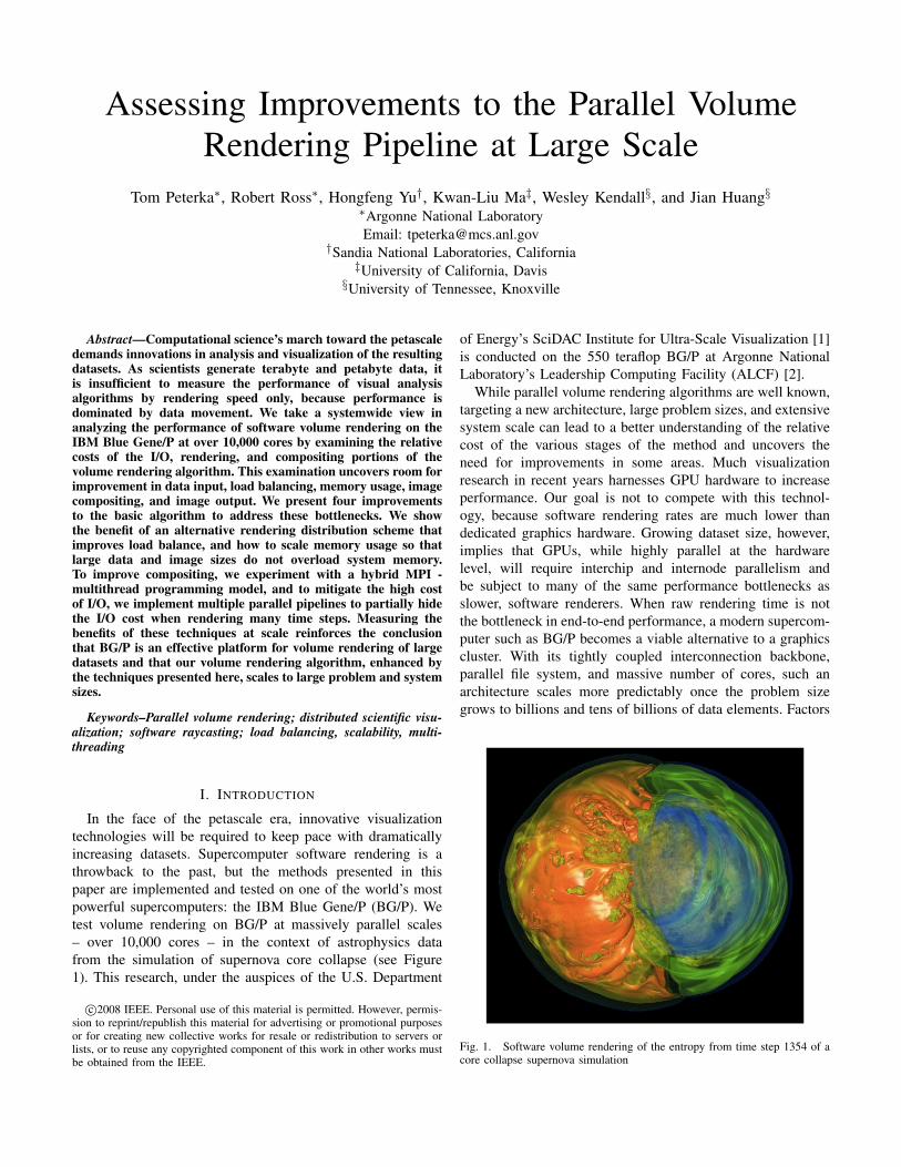
In the face of the petascale era, innovative visualizationtechnologies will be required to keep pace with dramaticallyincreasing datasets. Supercomputer software rendering is athrowback to the past, but the methods presented in thispaper are implemented and tested on one of the world’s mostpowerful supercomputers: the IBM Blue Gene/P (BG/P). Wetest volume rendering on BG/P at massively parallel scales– over 10,000 cores – in the context of astrophysics datafrom the simulation of supernova core collapse (see Figure1). This research, under the auspices of the U.S. Department

c©2008 IEEE. Personal use of this material is permitted. However, permis-sion to reprint/republish this material for advertising or promotional purposesor for creating new collective works for resale or redistribution to servers orlists, or to reuse any copyrighted component of this work in other works mustbe obtained from the IEEE.

of Energy’s SciDAC Institute for Ultra-Scale Visualization [1]is conducted on the 550 teraflop BG/P at Argonne NationalLaboratory’s Leadership Computing Facility (ALCF) [2].

While parallel volume rendering algorithms are well known,targeting a new architecture, large problem sizes, and extensivesystem scale can lead to a better understanding of the relativecost of the various stages of the method and uncovers theneed for improvements in some areas. Much visualizationresearch in recent years harnesses GPU hardware to increaseperformance. Our goal is not to compete with this technol-ogy, because software rendering rates are much lower thandedicated graphics hardware. Growing dataset size, however,implies that GPUs, while highly parallel at the hardwarelevel, will require interchip and internode parallelism andbe subject to many of the same performance bottlenecks asslower, software renderers. When raw rendering time is notthe bottleneck in end-to-end performance, a modern supercom-puter such as BG/P becomes a viable alternative to a graphicscluster. With its tightly coupled interconnection backbone,parallel file system, and massive number of cores, such anarchitecture scales more predictably once the problem sizegrows to billions and tens of billions of data elements. Factors

Fig. 1. Software volume rendering of the entropy from time step 1354 of acore collapse supernova simulation

such as I/O and communication bandwidth – not renderingspeed – dominate the overall performance.

The opportunity for in situ visualization [3] [4] [5], oroverlapping visualization with an executing simulation, isanother advantage associated with visualizing data on the samearchitecture as the simulation. Because postprocessing andtransporting data can dominate a scientific workflow as datasizes increase, moving the analysis and visualization closerto the data can be less expensive than the other way around.In situ techniques grow in importance as simulations grow insize. For example, Yeung et al. already routinely compute flowsimulations at 20483 data elements [6], and their next targetis 40963 using the IBM Blue Gene architecture. This equatesto approximately 270 GB per time step per variable. Similardataset sizes are currently being produced by Woodward et al.[7] in the area of fluid dynamics and by Chen et al. [8] inearthquake simulation.

In this paper we examine the costs of the various phases ofour volume rendering algorithm; I/O, rendering, and composit-ing as we scale the problem and system size. Based on ourfindings, we examine four improvements to the algorithm andstudy how each technique affects performance. The techniquesare: (a) load balancing via round-robin data block distribution,(b) memory conservation via parallel image output, (c) lever-aging shared memory architecture via hybrid programming,and (d) hiding I/O latency through multiple time step pipelines.While these techniques are not new inventions, we test themat scales up to 16K cores and analyze the benefit of each tothe whole as well as to individual parts of the parallel volumerendering algorithm.

II. BACKGROUND

A brief background on parallel volume rendering is followedby a survey of parallel performance in large scale visualization.This section concludes with a look at trends in modern parallelarchitectures and the changing programming models to supportthem.

A. Parallel Volume Rendering

Figure 2 shows that the a parallel volume rendering algo-rithm consists of three main stages: I/O, rendering, and com-positing. Each core executes I/O, rendering, and compositingserially, and this set of three operations is replicated in parallelover many cores. In the I/O stage, data are simultaneouslyread by all cores. The middle section, rendering, occurs inparallel without any intercore communication. The third stage,compositing, requires many-to-many communication using thedirect-send method [9]. Finally, a completed image from apipeline is either saved to disk or streamed over a network.

Sort-last parallel rendering methods [10] such as ours ac-commodate large data by dividing the dataset among nodes[11]. This approach can cause load imbalance in the renderingphase because of variations in scene complexity. Althoughit may seem that empty blocks should be fastest, the oppo-site is true in this algorithm. Early ray termination causescomputation of the volume rendering integral along a ray

Fig. 2. Functional diagram of the parallel volume rendering algorithm

to terminate once a maximum opacity is reached, but emptyregions never reach this maximum opacity and are evaluatedfully. Load imbalances occur only in the rendering phase; thecompositing phase is inherently load balanced by dividing theresulting image into uniform regions such as scan lines [12].Approaches to load balancing in the rendering phase can beeither dynamic [13] or static [14], and distribution can occurin data space, image space, or both [15].

B. Performance

To measure performance, we compile the time requiredfor each of the three stages in Figure 2, which sum to thetotal frame time, or the latency between viewing one timestep to the next. (Frame rate is the reciprocal of frame time.)The relative costs of the three phases shift as the number ofcores increases, but ultimately the algorithm is I/O bound [16].Rendering performance scales linearly assuming perfect loadbalance, because it requires no interprocess communication.Cost of the direct-send compositing portion of the algorithmis dominated by many-to-many communication and becomesa significant factor beyond 2K cores and eclipses renderingtime beyond 8K cores.

We do not use compression or multiple levels of detail,which can impose load imbalance and degrade visual quality.We do not preprocess the data to detect empty blocks, nor dowe hierarchically structure the data as in [17]. Because ourdata are time varying, we attempt to simply visualize “on-the-fly,” without doing any preprocessing between time steps.

In [18], Peterka et al. tested scalability up to 4K coresand concluded that leadership class supercomputers are viablevolume rendering platforms for large datasets, that I/O costdominates performance and must be mitigated, that renderinginefficiency is caused by load imbalance, and that compositingstrategies such as direct-send cannot scale indefinitely. Tosummarize some other large visualization results, we survey afew notable examples from the literature in Table I.

From this list, one may conclude that it is possible to visual-ize structured meshes of 1 billion elements at interactive ratesof several frames per second, including I/O for time varyingdata. Unstructured meshes can be visualized in tens of seconds,excluding I/O and preprocessing time. Large structured meshesof tens of billions of elements fall in between, requiring severalseconds excluding I/O time. Lighting is typically not possibleat these performance levels, and image sizes are usuallylimited to 1 megapixel. Our goal is to show scalability ratherthan interactive rates, but performance cannot be neglected

TABLE IPREVIOUSLY PUBLISHED LARGE VOLUME RENDERING RESULTS

Dataset BillionEle-ments

Mesh Type ImageSize

Time(s)

I/Oincl.

Ref.

MolecularDynamics

.14 unstructured 1Kx1K 30 no [19]

Blast Wave 27 unstructured 1Kx1K 35 no [19]Taylor-Raleigh

1 structured 1Kx1K 0.2 yes [20]

Fire 14 unstructured 800x800 16 no [21]

either. Our results will demonstrate that the performance ofthis method fits within the context of the work in Table I. Forexample, we will show that 11 billion elements on a structuredgrid can be volume rendered, with lighting, in 16 seconds,including I/O.

C. Parallel Architectures and Programming Models

In addition to passing messages between nodes, sharingmemory among cores is another way to achieve concurrency.Multicore architectures are ubiquitous today as chip makersstrive to satisfy Moore’s Law without the ability to increaseclock speed and power indefinitely. Parallel graphics andvisualization is evolving with this changing hardware. Forexample, Santos et al. [22] remark that the parallel visual-ization community began to address these architectures in2007. [23] is one such paper that specifically targets multicorearchitectures to perform quality interactive rendering of largedata sets. This trend continues in 2008 with many morepapers targeting multicore hardware, for example, volumerendering on the cell broadband engine [24]. The number ofcores in the Blue Gene PowerPC processor has doubled inthe last generation of machines, and this trend is likely tocontinue. These hardware changes suggest that programmingmodels will evolve to best harness the intra- and internodeparallelism that is available. MPI has been the de facto parallelprogramming model for many years, but OpenMP [25], IntelThread Building Blocks [26], and other libraries are gainingpopularity for writing multithreaded programs.

III. METHOD

In this section we elaborate on details of the implementa-tion. We begin by describing the nature of the dataset andBG/P architecture. We then discuss the program parametersthat vary in order to generate results, and discuss how perfor-mance data are collected and analyzed.

A. Dataset

Our datasets originate from Anthony Mezzacappa of OakRidge National Laboratory and John Blondin of North Car-olina State University and represent physical quantities duringthe early stages of supernova core collapse [27]. Variablessuch as density, pressure, and velocity are stored in netCDF[28] file format, in structured grids of size 8643 and 11203.The two data sizes contain 0.65 and 1.4 billion elements pertime step, respectively. Additionally, we created two simulatedlarger datasets by doubling each of the actual datasets in three

dimensions. These simulated data are eight times larger thanthe original, or 5.2 and 11.2 billion data elements, respectively.In order to visualize the data, each time step is preprocessedto extract a single variable from the netCDF file and writtenin a separate file in 32 bit floating point format. With asingle variable extracted, the file sizes for one time step ofthe actual and simulated datasets are 2.6, 5.6, 20.8, and 44.8GB, respectively.

B. Architecture

Argonne National Laboratory’s Leadership Computing Fa-cility (ALCF) [2] operates a 557 teraflop (TF) BG/P super-computer. Four PowerPC450 cores that share 2 GB of RAMconstitute one BG/P node. Peak performance of one core is3.4 gigaflops (GF), or 13.6 GF per node. One rack contains1K nodes (4K cores), has 2 TB memory, and is capable of13.9 TF peak performance. Eight racks equate to 16 TB RAMand 108 TF. The complete system contains 40 racks (40Knodes, 160K cores) 80 TB RAM, with peak performanceof 557 TF. These relationships are diagrammed in Figure 3.IBM provides extensive online documentation of the BG/Parchitecture, compilers, and users’ and programmers’ guides[29].

C. Program Parameters

We built many controls into the volume rendering applica-tion. For example, the image mode is variable: not just thesize of the finished image but whether it is saved to a file orstreamed to a remote display. The number of time steps runin succession, including looping indefinitely over a finite timeseries, can be set. Lighting can be enabled or disabled; weenable lighting in order to demonstrate performance for highquality rendering. The density of point sampling along eachray can be controlled with a parameter as well.

A few more controls govern the arrangement of processesinto parallel pipelines, multiple threads, and collective writers.The number of pipelines is variable up to the limit of thetotal number of cores available. For example, 8K cores can be

Fig. 3. Argonne’s BG/P architecture.

TABLE IISAMPLE PROGRAM PARAMETERS

Parameter Example NotesDataSize 11203 Grid size (data elements)ImageSize 16002 Image size (pixels)NumProcs 16384 Total MPI processesNumPipes 16 16 pipelines of 1K processes eachNumThreads 1 Threads per MPI processNumNodes 4096 BG/P nodes (eg, vn mode)NumWriters 64 Parallel image output processesBlockingFactor 8 Round-robin data blocks per process

configured in a single pipeline, two pipes of 4K cores each, etc.The rendering portion of an MPI process can be multithreadedwith up to four POSIX pthreads. Each pipeline can output thefinal image in parallel, using a number of writer processes.Table II lists a sample of the parameters used to control thevolume rendering code. With these parameters, the test setupis flexible and configurable. The meaning of most of theseparameters will be clear when they are used to generate theresults in Section IV.

D. Emphasis on Quality

It is important for visualizations of scientific data to faith-fully replicate detail and provide the highest fidelity, mostenlightening view of the data possible. For example, when dataare computed at high spatial resolution, high image resolutionshould be used to view the result so that the image area iscomparable to the view area of the data volume. Besides imagesize, careful choice of ray sample spacing and the use oflighting models affect the quality of output images.

Lighting and shading add a high degree of informationcontent and realism to volume rendering. For example, com-pare the two images of supernova angular momentum withand without lighting in Figure 4. The illuminated model,complete with specular highlights, resembles the appearanceof isosurface rendering. This quality comes at a price, andalthough straightforward to compute, interactive volume ren-derers often omit lighting in order to maintain frame rate.With the extended potential for scaling that leadership classmachines offer, we compute lighting as a matter of course. Byestimating gradient direction from differences of neighboringvertex values, a normal direction is calculated on the fly foreach data point, and a standard lighting model, includingambient, diffuse, and specular components, is computed [30].

Just as image size should be proportional to the length andwidth of the data volume, the sample spacing along each rayshould be of the same order as the volume data spacing in thedepth direction. This way, larger, higher resolution data arereproduced faithfully. Our algorithm generates samples alongrays spaced at an adjustable fraction of the data spacing. Wealways set this parameter to one. Thus, the number of samplesalong each ray grows or shrinks with the number of datavoxels, ensuring that image acuity matches data detail.

IV. RESULTS

This section quantifies gains from our main improvementsto the volume rendering algorithm: load balancing, parallel

Fig. 4. Unlit (top) rendering vs. lit (bottom) rendering. Image quality thatresembles triangle mesh isosurfacing can be produced with direct volumerendering.

output, multithreaded rendering, and parallel pipelines. Testson large data and high numbers of cores validate the results.

A. Load Balancing

Load balancing is a difficult problem when it is in thecontext of large problem sizes, large numbers of cores, andtime varying data. Uniform load balance is crucial to goodscalability and efficiency, and much research has been pub-lished in this area of parallel computing. However, many ofthe published methods do not scale, particularly their commu-nication costs, to thousands of cores under the performanceconstraints of time dependant data. Marchesin et al. [13]provide a dynamic load balancing method that requires data tobe replicated on all cores; data replication is unacceptable forour problem scale. Childs et al. [19] describe a two phaserendering algorithm that balances work load by dividing aportion of it within object space and the rest in image space,but the cost of an additional many-to-many communication

Fig. 5. Efficiency of the rendering phase can be improved by distributingdata blocks in a more equitable manner. Round-robin balancing assigns manyblocks to each core, distributed in a round-robin fashion. Compare efficiencythe default distribution of one block per core.

Fig. 6. There is additional I/O cost associated with round robin, since eachprocess must read many more noncontiguous blocks. However, this cost isoffset by increases in rendering efficiency.

between the two stages may be prohibitive for our purposes.Ma et al. [31] show good scalability and parallel efficiencythrough a round-robin static distribution method.

Choosing a low cost but effective strategy, we implementedand tested the round-robin approach. Round-robin data par-titioning is inexpensive because it is still a static balancingscheme but it has a good probability of achieving a roughlyuniform load balance. The dataset is divided into more blocksthan processors and the blocks are assigned to processors ina round-robin fashion. The number of blocks per processor iscalled the blocking factor: we have found 4, 8, or 16 to besufficient for most cases.

The round-robin load distribution is surprisingly effectivefor increasing rendering efficiency, especially considering itslow cost. Occasionally we need to hand tune the blockingfactor to increase efficiency further. For example, in our testswe found 32 blocks per process to be better at 128 and 256cores, but we can now smooth out previous bumps in efficiency

curves easily through appropriate choice of blocking factor.Figure 5 compares rendering efficiency with and withoutround-robin balancing. The default case represents the uniformdata division into the same number of blocks as processors.The round-robin case represents the improved load balancescheme.

Figure 5 shows that the round robin distribution is notperfect. For example, there are instances such as 512 and4K cores where the default distribution is coincidentally verygood, reaching over 90%. On average, however, the round-robin distribution is more predictable and in most casesbetter than the default, ranging between 70 and 90% overseveral thousand cores. The raw rendering time shows thisimprovement as well, completing faster than before in mostcases. There is an I/O cost, however, in reading a number ofnonadjacent blocks sequentially within each process, insteadof just one or sometimes two. See Figure 6, which measuresthe I/O portion of time only. In all but two cases, however,the increase in I/O time was offset by a reduction in renderingtime.

In those cases where the increased I/O cost remains, wewill show later that I/O can be hidden effectively throughmultiple pipeline parallelism. Another potential optimizationis to write a more intelligent I/O read function that batchesthe sequential reads that a process makes into a higher levelcollective read that can occur simultaneously. MPI-IO dictatesthat any collective file I/O operations occur in monotonicallynondecreasing byte order at the file level. Hence, blocks inthe subvolume would need to be decomposed into stringsof contiguous bytes, and these strings sorted with respect tofile byte order. Then a processes can read all of its blockscollectively, followed by reassembly into subvolume blocksonce in memory. We are considering implementing this in thefuture.

To further test the overall performance of the algorithmwith load balancing, we present overall timing results for fourdata sizes, 8643, 11203, 17283, and 22403. The first two sizesare the actual data from Blondin et al.’s computational runs.

Fig. 7. The total frame rate with lighting is plotted for the 11203 dataset.

Fig. 8. At large data sizes and many cores, the relative contributions of thethree stages of the algorithm are dominated by I/O. Compositing cost alsogrows.

We generated the latter two sizes by doubling the size of theoriginal datasets in each direction, producing a file size eighttimes as large as the original.

The 11203 time step contains 1.4 billion data values. Figure7 shows total frame rate (including I/O) for this data size, asa function of the number of cores. The total frame time at 8Kcores is 7.9 s. Blocking factors for the round robin distributionrange from 16 at lower numbers of cores to 4 at the upper end.The slope of the curve gradually decreases as compositing costgrows with increased numbers of cores.

For the same test conditions in Figure 7, Figure 8 shows thedistribution of time spent in I/O, rendering, and compositing.I/O dominates over the vast majority of the plot, and at8K cores compositing is nearly as expensive as rendering.Extrapolating these these trends further out, rendering will bethe least expensive of the three stages beyond approximately10K cores. At the far right side of the time distribution, therelative percentage of I/O decreases. This is caused by theincreasing cost of compositing, not because the I/O rate itselfimproved.

The total, end-to-end times for all four data sizes are listedin Table III. For comparison to other published results, we alsoinclude the visualization-only time in the right-hand column;this is the rendering time plus the compositing time, excludingI/O time. The image size is a constant 10242 pixels for thesetests. At the scale of 16K cores, rendering has become thefastest of the three stages and compositing has grown to nearly30% of the total frame time. Data movement, whether networkcommunication or storage access, dominates the process at

TABLE IIISIMULATED LARGE DATA SIZES

GridSize

Elements(billion)

File Size(GB)

Cores End-EndTime (s)

Vis-OnlyTime (s)

8643 .64 2.4 2K 3.6 0.811203 1.4 5.2 8K 7.9 2.417283 5.2 19.2 16K 15.6 5.222403 11.2 41.9 16K 16.4 5.2

large scale.

B. Memory Conservation Through Parallel Writers

Memory is a scarce resource on BG/P. As we saw in SectionIII.B, 2GB are divided among 4 cores, or 512 MB per core invirtual node mode. Even though the compute node kernel onlyrequires a few megabytes, it is still easy for an application toexceed the remaining 510 megabytes or so. Applications mustconserve memory.

The size of the data and the size of the image both determinehow much memory is required by the volume rendering appli-cation. Memory requirements grow with problem size; that isunavoidable. We must ensure, nonetheless, that the amount ofrequired memory decreases linearly with the number of cores,so that large problems can fit into memory by allocating morecores. Otherwise, the program will run out of memory at somedata or image size, regardless of the number of cores.

That was exactly our situation. Even after optimizingmemory usage to dynamically grow memory buffers onlyas needed, an underlying problem remained: the entire im-age needed to eventually reside on one core at the end ofthe process. The data structure that accompanies each rayrequires significant memory per pixel, much more than justthe R,G,B,A color values. The compositing process concludeswith an MPI Gatherv() operation that funnels all of thecompleted subimages to one core. This core tessellates thepieces into one image and saves it to disk. This serialization isa choke point in the algorithm. Performance suffers, memoryusage does not scale, and image sizes beyond 16002 pixelscrash the program.

The solution is to write images out in parallel with MPI-IO at the end of the algorithm, similar to the way thatdata are read in parallel at the start of the algorithm. Forperformance reasons, we want to control how many writingcores (“writers”) we use. Too few writers result in the situationdescribed previously. Too many writers hinder performance,

Fig. 9. The tail end of the algorithm consists of three substages: compositing,gathering down to a possibly smaller number of writers, and collectivelywriting the image to disk. Parallel image output is more scalable in termsof memory usage. No core needs to allocate space for the entire image, alongwith its associated data structures.

because each writer writes very little. In this discussion andin Figure 9, terms such as writers, renderers, and compositorsrefer to the roles certain processes play at a given time. Thesame process takes on different roles during various stages ofthe algorithm. All processes act as renderers and compositors;later, a subset of processes become writers during the laststage.

We implemented a flexible scheme diagrammed in Figure9. By creating several MPI communicators, compositing isfollowed by a partial gather down to the desired number ofwriters, and concludes with a collective image write to disk.Because the number of writers is a parameter, it can be anyvalue from one to the total number of cores. Figure 10 showsthat the optimal number of writers is 64 for this example. Thistest included 2 K cores, the 11203 dataset, and an image sizeof 20482 pixels.

In fact, now that memory is more scalable, we have success-fully generated images as large as 40963, or 16 megapixels.After these improvements, the final memory usage model forthis algorithm is:

m = 70M + 2.5Kp/c + 4v/c

Where:

1) m is the total memory usage in bytes2) p size is the total number of pixels in the image3) v is the total number of data elements in the volume4) c is the total number of cores being used5) M, K are one megabyte and one kilobyte, respectively

In this model, the memory requirements for data size andimage size are divided by the number of cores. 70 MB areallocated by the MPI library, but we can control the rest ofthe memory usage by applying more or fewer cores to thevolume rendering task.

Fig. 10. Different numbers of writers affect overall output performance.We divide this stage into three substages: composite, gather, and write. Thestacked graph shows the relative time that each of these substages takes whenthe number of writers is varied. 2 K compositors are used, and the image sizeis 20482 pixels.

Many data structures depend on the image size, includingray casting, compositing schedule, and the partial image itself.That is why the coefficient of p is so much larger than thatof v. However, v itself is generally three orders of magnitudelarger than p, so both image and data size end up contributingto the memory usage. We tested the accuracy of this modelbetween 256 and 1024 cores, image sizes from 2562 to 20482,and volume sizes up to 11203.

C. Hybrid MPI - Multithreaded Rendering

Multicore computer architectures are ubiquitous today.BG/P is no exception: each node contains four cores that canbe operated individually (virtual node mode), in pairs (dualmode), or as one unit (SMP mode). In SMP mode, 2 GBof memory constitute a common address space that is sharedamong the four cores. Thus far, we have not attempted toexploit this mode of operation, limiting ourselves to virtualnode mode where each core acts as a separate processor withits own process space of 512 MB. With current architecturestending toward multi and many cores, however, it is necessaryto develop new programming models that can exploit changingtechnology. We were curious what advantages could be gainedby combining message passing and shared memory parallelismin our volume renderer. As usual, we wanted to test this atlarge system scale, so we modified a portion of the volumerendering code to include a hybrid multithreaded / MPIcomponent, with the goal of measuring how the I/O, rendering,and compositing time compared to the original.

We changed the rendering portion of the volume rendereronly, dictating whether an MPI process runs the renderingstage with one thread or with 4 threads within that process.In the first case, one process per core executes in virtual nodemode, while in the second case, one process per node executesin SMP mode. BG/P’s microkernel statically maps each ofthe four threads to one of the four cores within the node.Several programming APIs are available for thread manage-ment, including OpenMP and POSIX pthreads. We chose thelatter for simplicity: thread creation was straightforward withpthreads and there was no scheduling advantage that OpenMPcould provide within the context of BG/P’s static allocation ofthreads to cores. In the following performance graphs, the firstcase is labeled “4 procs” (processes) while the second case islabeled “4 threads.” “4 procs” implies the conventional MPI-only method and “4 threads” is the hybrid MPI - multithreadmethod.

In the 4 threads method, the distribution of data space andimage space is hybrid as well as the programming model.Among nodes and MPI processes, the data space is still dividedinto blocks, but among threads within a node, the image spaceis divided into 4 image regions. Ray casting is a naturalalgorithm to parallelize in image space, because each ray isindependent of the others. The threads do not communicatewith one another and the results of the cast rays are writtento different addresses in the same data structure without needfor synchronization or mutual exclusion. The only restriction

Fig. 11. Top: I/O and composite time vs. number of nodes when rendering isperformed with 4 processes per node and 4 threads per node. Bottom: Similartest of rendering time. Rendering can be adversely affected by load imbalance,as the “4 threads (unbalanced)” curve shows.

is that all four threads complete the rendering stage before theprogram can proceed to the next stage, compositing.

When plotting results, we align values along the horizontalaxis based on the same physical number of BG/P nodes,to enable a fair comparison. This way, the physical amountof hardware is the same. Some of the results matched ourexpectations, while others were a surprise. We predicted thateven though the rendering step is where the code was changed,the rendering time should remain roughly constant in bothscenarios. The total number of rays to be cast is the same,and since rendering requires no communication between eitherprocesses or threads, there should be little difference betweenthe two approaches. On the contrary, we predicted that theI/O and compositing steps would be affected by the way thatthe program is executed. In virtual node mode, there are fourtimes as many processes performing collective reading andfour times as many participants exchanging messages.

Figure 11 shows our results for a test of one time stepof the 11203 dataset, rendered to a 10242 pixel image. Bothgraphs compare aspects of the two programming models as thenumber of nodes increases. The top graph illustrates I/O andcompositing time while the bottom graph depicts renderingtime. The I/O time did not improve much with multithreading.

At higher numbers of nodes, one might expect to see someI/O improvement because the dataset is divided into fewer,larger blocks. However, storage traffic passes through the samenumber of I/O nodes in BG/P, irrespective of the number ofprocesses per compute node. Furthermore, MPI-IO executescollective I/O calls with the help of “aggregators.” These canbe thought of as a smaller number of actors that actually carryout I/O requests on behalf of MPI processes. The numberof aggregators is also based on the number of I/O nodes,usually eight per I/O node, and this is a way for MPI-IO toavoid small, individual reads by grouping them into larger sets.These factors appear to have more significant impact on I/Orates than the changes that we made to the code.

The real win is in compositing. With fewer numbers ofprocesses that need to exchange messages, compositing perfor-mance begins to improve at 128 nodes. With multithreading,the hybrid division of labor into both data space and imagespace takes advantage of the natural parallelism in ray casting.Rays within the same node exchange no information, andmultithreading allows four subsets of rays to be computed inroughly the same time. This is the ideal parallel scenario. Thecompositing curves in the upper graph of Figure 11 show thisimprovement.

The lower graph confirms our hypothesis that rendering timedoes not improve with programming model, but it reveals asurprising fact. While multithreading did not speed up render-ing, it can degrade rendering performance if not done carefully.We see that the “4 procs” and “4 threads” performance isvirtually identical, except for minor deviations at 32 and 64nodes. However, we also include a “4 procs unbalanced”result that is substantially slower. The cause of this slowdown,as the name suggests, is load imbalance between the fourthreads. Since all four threads must join before proceedingto compositing, the slowest thread dictates performance forthe node. There is little to be gained from concurrency if thethreads are imbalanced. As the lower graph shows, this canactually be slower than the MPI-only case, which has no suchbarrier per node.

Fortunately, we already solved this problem in anothercontext. We can achieve interthread load balance using assimilar technique as in Subsection A: round-robin distribution.This time, the distribution is in image space, but the idea isthe same. Each thread operates on more than one region ofthe image, and those regions are interleaved in round-robinfashion. We call these regions stripes, and found that a stripingfactor of eight stripes per thread was sufficient to balancerendering load. The curve labeled “4 threads” in the bottomgraph of Figure 11 is generated with eight stripes per thread.The interleaving of threads and stripes within a subimagefollows the pattern below:

• Thread 0, Stripe 0• Thread 1, Stripe 0• Thread 2, Stripe 0• Thread 3, Stripe 0• Thread 0, Stripe 1• ...

• Thread 3, Stripe 8

D. Multiple Parallel Pipelines

The previous sections demonstrate good scalability, but theyalso point out two problems. One is the diminishing returnfrom higher numbers of cores in Figure 7, and the other is thewidening gap between visualization-only time and end-to-endtime in Table 2. Rendering time is not the bottleneck at scale:I/O dominates the frame time and further progress dependson hiding this I/O cost. In a time varying dataset, we cannotchoose to simply ignore I/O time when measuring the framerate because each time step or image frame requires a newfile to be read. The I/O cost, however, can be mitigated andeven completely hidden if sufficient I/O bandwidth, renderingresources, and communication bandwidth exist to processmultiple time steps simultaneously.

The solution is two levels of parallelism: inter- time step andintra- time step parallelism using multiple parallel pipelines.In fact, even some of the rendering costs can be absorbed ifthe pipelines have sufficient overlap. As long as final framesare sent out in order, the client display software can bufferframes to smooth out any discrepancies in interframe latencyand present final frames at a consistent frame rate.

Collections of cores are grouped into parallel pipelines [31].Within any pipeline, many cores operate in parallel. Figure12 shows a simplified diagram of a multipipe architecturefor this application with four pipelines. Each pipeline isactually a collection of many cores operating in parallel onthe same time step. The boxes are labeled I/O for file reading,R for rendering, and C/S for compositing and sending. Allfour pipelines begin at the same time because there is noneed to synchronize them until the final stage. The onlysynchronization requirement is that images are output in order.

We can also impose further serialization within the pipelineinterior, so that only one pipeline has control of the storageor communication network at any time. We call this a stagedpipeline. It imposes a higher degree of serialization in ex-change for less contention. An unstaged pipeline allows themaximum parallelism without concern for contention, orderingonly the final sending of the resulting images. In our tests,staging of I/O or compositing did not significantly affect theframe time, but we have retained the staging feature in thecode and will retest whether this has an effect at still largerscales.

Some idle time may occur within each pipe between thecompletion of rendering (R) and the start of either compositingor sending (C/S). This depends on the exact sum of thecomponent times with respect to the number of pipelines. Inthe limit, however, multiple pipelines can reduce the frametime from the sum of I/O + R + C/S to just the C/S time, asignificant savings.

Figure 13 shows the results of our experiments with 1, 2,4, 8, and 16 pipelines arranged as follows:

• 1 pipe of 8 K cores• 1 and 2 pipes of 4 K cores• 1, 2, and 4 pipes of 2 K cores

• 1, 2, 4, and 8 pipes of 1 K cores• 1, 2, 4, 8, and 16 pipes of 512 coresThe frame rate in Figure 13 is measured at the receiving dis-

play device; images are streamed to it as they are completed.An average frame rate is computed over all of the time stepsreceived, so this is an end-to-end value that includes the entiresystem including I/O, rendering, compositing, and streaming.No compression is used for streaming or elsewhere in thesetests. The graph shows five curves of various size pipelines,512 to 8192 cores per pipeline. The horizontal axis shows thetotal number of cores used in the test. The number of pipelinesfor a given data point is the total number of cores divided bythe number of cores per pipeline.

Performance improves along each curve with each doublingof the number of pipes. In fact, with 512 cores per pipe, theframe time (reciprocal of the frame rate) improved from nearlyeighteen seconds for a single pipe to just over one second forsixteen pipes. At this point all of the I/O time is hidden alongwith a portion of the original single-pipe visualization time.

Figure 13 also demonstrates that performance improves forthe same total number of cores, depending on how manypipelines they are arranged into. For example, 8K total coresarranged as 16 pipes of 512 cores produces a frame rate thatis six times faster than 8K cores in a single pipe. Intersectingthe curves of 13 with any vertical grid line produces a similarresult: for a constant total number of cores, faster timesare attained by arranging the cores into a greater numberof smaller size pipelines. We conclude that the overlap ofoperations in Figure 12 contributes more than simple scalingof the number of cores because the total end-to-end time isI/O bound and does not scale linearly. In other words, hidingthe I/O time via multiple pipelines is an effective tool tocounterbalance I/O cost.

V. DISCUSSION

By improving load balancing, conserving memory throughparallel output, combining MPI with multithreaded program-

Fig. 13. Multiple pipelines can provide several times faster performance,even if the same total number of cores is distributed into several pipes insteadof a single pipe.

Fig. 12. Example of how four parallel pipelines can reduce frame time and hide I/O cost. I/O = file read, R = render, C/S = composite and send.

ming, and employing multiple pipelines, we have extended thescale of high quality time varying volume rendering to over 10billion data elements per time step. By scaling to over 10,000cores, we can generate results at frame times on the order ofseveral seconds, including I/O and lighting.

A simple round-robin load distribution scheme achieves twotimes better balance than naive single-block allocation. Withextreme numbers of cores, this may be the best that canbe achieved without the cost of load balancing outweighingits benefit. More complex redistribution of data at thesescales, within performance constraints, has yet to be achieved.Even round-robin distribution carries increased I/O costs, butthese can be offset through improved rendering efficiency andmultipipe parallelism.

Changes in memory allocation can extend the scalabilityof our volume renderer. By outputting the image in parallel,memory use scales inversely with the number of renderingcores. Now, arbitrarily large volumes and images can beaccommodated by allocating enough cores to the problem. Weimplemented this feature using several MPI communicatorsand gathering the number of compositors down to a smallernumber of writers. By making the number of writers a programparameter, we can test variable numbers of writers, from oneto the total number of cores.

Computer architectures are becoming increasingly multi-core. Another way to improve the performance of parallelmachines is to exploit the intranode parallelism that exists onchip. By allocating one MPI process per node and one threadper core for the rendering portion of the algorithm, we havefound that a hybrid programming model can increase the I/Oand compositing performance at large system scale. Render-ing cost remains approximately constant whether threads orprocesses are used, but the overall program performance canimprove due to the improvements in the other parts of thealgorithm.

The multiple pipeline organization effectively hides I/Ocosts in time varying datasets by processing multiple timesteps simultaneously. It is often more efficient to arrange afixed number of cores into more pipelines of fewer cores each,than to group all of the cores into a single pipeline.

With these improvements, it is technically feasible to applyleadership-class machines at large scales to visualization andanalysis problems such as volume rendering. The remainingquestion is, “Is this use of resources justified?” While such

nontechnical questions are outside of the scope of this re-search, the remainder of this section presents a few argumentswhy we believe that this use of valuable resources is desirable,justifiable, and surprisingly economical. Foremost, we arecreating the foundation for in situ visualization. Not onlydoes this offer significant savings in terms of time and datamovement, but having access all of the simulation data insitu affords new capabilities, such as simultaneous analysisof multiple variables. Interacting with the simulation, notjust the visualization, is another advantage. Numerous otherpossibilities exist in this exciting new research area.

In order to faithfully resolve detail in large datasets, largedisplay devices such as tiled walls and accompanying largeimage sizes (tens and hundreds of megapixels) are required.Otherwise, the display size and image resolution effectivelydown-sample the dataset to a much coarser level of detail.Data are discarded just as if the dataset had originally beenmuch smaller, except that information is discarded at the endof a potentially long and expensive visualization workflow.Larger display and image sizes require orders of magnitudelarger visualization systems than are currently available inthe graphics cluster class of architectures. Leadership-classmachines are currently the only choice when considering notonly large data size, but also high image resolution.

In terms of scheduling and machine utilization, in ourexperience, visualization jobs interleave easily within othercomputational runs. Our visualization runs are short, usuallyonly a few minutes. Over the course of a week, these short runsaccrue no more than a few hours of total CPU time. Even if16K cores are required for a total of 10 hours per week (morethan we have used to date), this is still only a fraction of onepercent of the utilization of a 500 TF machine. A job schedulercan back-fill the unused cycles between scheduled computa-tional runs with analysis and visualization tasks. These cycleswould be wasted otherwise, so the visualization is essentiallyfree.

VI. FUTURE WORK

We continue to scale up to larger data and more cores. In sodoing, new bottlenecks appear. The next hurdle to overcomerequires rewriting the compositing part of the algorithm toemploy binary swap [32]. More efficient compositing is oneof the priorities for successful operation at tens of thousandsof cores.

Improving I/O performance is another. The ALCF re-searchers continue to improve aggregate I/O bandwidth andI/O scalability; these improvements are welcome because theydirectly affect the performance of this application. We areinvestigating different I/O file formats and ways to increasethe aggregate I/O bandwidth of our application as well.

ACKNOWLEDGMENT

We thank John Blondin and Anthony Mezzacappa formaking their dataset available for this research. This workwas supported by the Office of Advanced Scientific ComputingResearch, Office of Science, U.S. Department of Energy, underContract DE-AC02-06CH11357. Work is also supported inpart by NSF through grants CNS-0551727, CCF-0325934, andby DOE with agreement No. DE-FC02-06ER25777.

REFERENCES

[1] (2008) Scidac institute for ultra-scale visualization. [Online]. Available:http://ultravis.ucdavis.edu/

[2] (2008) Argonne leadership computing facility. [Online]. Available:http://www.alcf.anl.gov/

[3] K.-L. Ma, C. Wang, H. Yu, and A. Tikhonova, “In-situ processing andvisualization for ultrascale simulations,” Journal of Physics, vol. 78,2007.

[4] T. Tu, H. Yu, L. Ramirez-Guzman, J. Bielak, O. Ghattas, K.-L. Ma, andD. R. O’Hallaron, “From mesh generation to scientific visualization: Anend-to-end approach to parallel supercomputing,” in Proc. Supercomput-ing 2006, Tampa, FL, 2006.

[5] H. Yu, K.-L. Ma, and J. Welling, “A parallel visualization pipeline forterascale earthquake simulations,” in Proc. Supercomputing 2004, 2004,p. 49.

[6] P. K. Yeung, D. A. Donzis, and K. R. Sreenivasan, “High-reynolds-number simulation of turbulent mixing,” Physics of Fluids, vol. 17, no.081703, 2005.

[7] P. Woodward. (2008) Laboratory for computational science andengineering. [Online]. Available: http://www.lcse.umn.edu/index.php?c=home

[8] L. Chen, I. Fujishiro, and K. Nakajima, “Optimizing parallel per-formance of unstructured volume rendering for the earth simulator,”Parallel Computing, vol. 29, no. 3, pp. 355–371, 2003.

[9] U. Neumann, “Communication costs for parallel volume-rendering al-gorithms,” IEEE Computer Graphics and Applications, vol. 14, no. 4,pp. 49–58, 1994.

[10] S. Molnar, M. Cox, D. Ellsworth, and H. Fuchs, “A sorting classificationof parallel rendering,” IEEE Computer Graphics and Applications,vol. 14, no. 4, pp. 23–32, 1994.

[11] B. Wylie, C. Pavlakos, V. Lewis, and K. Moreland, “Scalable renderingon pc clusters,” IEEE Computer Graphics and Applications, vol. 21,no. 4, pp. 62–69, 2001.

[12] A. Stompel, K.-L. Ma, E. B. Lum, J. Ahrens, and J. Patchett, “Slic:Scheduled linear image compositing for parallel volume rendering,” inProc. IEEE Symposium on Parallel and Large-Data Visualization andGraphics, Seattle, WA, 2003, pp. 33–40.

[13] S. Marchesin, C. Mongenet, and J.-M. Dischler, “Dynamic load balanc-ing for parallel volume rendering,” in Proc. Eurographics Symposium ofParallel Graphics and Visualization 2006, Braga, Portugal, 2006.

[14] K.-L. Ma and T. W. Crockett, “A scalable parallel cell-projection volumerendering algorithm for three-dimensional unstructured data,” in Proc.Parallel Rendering Symposium 1997, 1997, p. 95.

[15] A. Garcia and H.-W. Shen, “An interleaved parallel volume renderer withpc-clusters,” in Proc. Eurographics Workshop on Parallel Graphics andVisualization 2002, Blaubeuren, Germany, 2002, pp. 51–59.

[16] H. Yu and K.-L. Ma, “A study of i/o methods for parallel visualizationof large-scale data,” Parallel Computing, vol. 31, no. 2, pp. 167–183,2005.

[17] J. Gao, C. Wang, L. Li, and H.-W. Shen, “A parallel multiresolutionvolume rendering algorithm for large data visualization,” Parallel Com-puting, vol. 31, no. 2, pp. 185–204, 2005.

[18] T. Peterka, H. Yu, R. Ross, and K.-L. Ma, “Parallel volume renderingon the ibm blue gene/p,” in Proc. Eurographics Parallel Graphics andVisualization Symposium 2008, Crete, Greece, 2008.

[19] H. Childs, M. Duchaineau, and K.-L. Ma, “A scalable, hybrid scheme forvolume rendering massive data sets,” in Proc. Eurographics Symposiumon Parallel Graphics and Visualization 2006, Braga, Portugal, 2006, pp.153–162.

[20] J. Kniss, P. McCormick, A. McPherson, J. Ahrens, J. S. Painter, A. Kea-hey, and C. D. Hansen, “Interactive texture-based volume rendering forlarge data sets,” IEEE Computer Graphics and Applications, vol. 21,no. 4, pp. 52–61, 2001.

[21] K. Moreland, L. Avila, and L. A. Fisk, “Parallel unstructured volumerendering in paraview,” in Proc. IS&T SPIE Visualization and DataAnalysis 2007, San Jose, CA, 2007.

[22] L. P. Santos, D. Reiners, and J. Favre, “Parallel graphics and visualiza-tion,” Computers and Graphics, vol. 32, no. 1, pp. 1–2, 2008.

[23] C. P. Gribble, C. Brownlee, and S. G. Parker, “Practical global illumi-nation for interactive particle visualization,” Computers and Graphics,vol. 32, no. 1, pp. 14–24, 2008.

[24] J. Kim and J. Jaja, “Streaming model based volume ray casting imple-mentation for cell broadband engine,” in Proc. Eurographics ParallelGraphics and Visualization Symposium, Crete, Greece, 2008.

[25] (2008) Openmp. [Online]. Available: http://openmp.org/wp/[26] (2008) Intel thread building blocks. [Online]. Available: http:

//www.threadingbuildingblocks.org/[27] J. M. Blondin, A. Mezzacappa, and C. DeMarino, “Stability of standing

accretion shocks, with an eye toward core collapse supernovae,” TheAstrophysics Journal, vol. 584, no. 2, p. 971, 2003.

[28] (2008) Netcdf. [Online]. Available: http://www.unidata.ucar.edu/software/netcdf/

[29] (2008) Ibm redbooks. [Online]. Available: http://www.redbooks.ibm.com/redpieces/abstracts/sg247287.html?Open

[30] N. L. Max, “Optical models for direct volume rendering,” IEEE Transac-tions on Visualization and Computer Graphics, vol. 1, no. 2, pp. 99–108,1995.

[31] K.-L. Ma and D. M. Camp, “High performance visualization of time-varying volume data over a wide-area network,” in Proc. Supercomput-ing 2000, Dallas, TX, 2000, p. 29.

[32] K.-L. Ma, J. S. Painter, C. D. Hansen, and M. F. Krogh, “Parallel volumerendering using binary-swap compositing,” IEEE Computer Graphicsand Applications, vol. 14, no. 4, pp. 59–68, 1994.

The submitted manuscript has been created by UChicagoArgonne, LLC, Operator of Argonne National Laboratory(“Argonne”). Argonne, a U.S. Department of Energy Officeof Science laboratory, is operated under Contract No. DE-AC02-06CH11357. The U.S. Government retains for itself,and others acting on its behalf, a paid-up nonexclusive,irrevocable worldwide license in said article to reproduce,prepare derivative works, distribute copies to the public, andperform publicly and display publicly, by or on behalf of theGovernment.