Embed Size (px)
Citation preview

ABSTRACT
Title of Dissertation: TACKLING UNCERTAINTIES AND ERRORS IN THE
SATELLITE MONITORING OF FOREST COVER CHANGE
Kuan Song, Ph. D, 2010
Directed By: Professor John R. G. Townshend
Department of Geography University of Maryland, College Park
This study aims at improving the reliability of automatic forest change detection.
Forest change detection is of vital importance for understanding global land cover as
well as the carbon cycle. Remote sensing and machine learning have been widely
adopted for such studies with increasing degrees of success. However,
contemporary global studies still suffer from lower-than-satisfactory accuracies and
robustness problems whose causes were largely unknown.
Global geographical observations are complex, as a result of the hidden
interweaving geographical processes. Is it possible that some geographical
complexities were not expected in contemporary machine learning? Could they
cause uncertainties and errors when contemporary machine learning theories are
applied for remote sensing?

This dissertation adopts the philosophy of error elimination. We start by
explaining the mathematical origins of possible geographic uncertainties and errors in
chapter two. Uncertainties are unavoidable but might be mitigated. Errors are
hidden but might be found and corrected. Then in chapter three, experiments are
specifically designed to assess whether or not the contemporary machine learning
theories can handle these geographic uncertainties and errors. In chapter four, we
identify an unreported systemic error source: the proportion distribution of classes in
the training set. A subsequent Bayesian Optimal solution is designed to combine
Support Vector Machine and Maximum Likelihood. Finally, in chapter five, we
demonstrate how this type of error is widespread not just in classification algorithms,
but also embedded in the conceptual definition of geographic classes before
classification. In chapter six, the sources of errors and uncertainties and their
solutions are summarized, with theoretical implications for future studies.
The most important finding is, how we design a classification largely
pre-determines the “scientific conclusions” we eventually get from the classification
of geographical observations. This happened to many contemporary popular
classifiers including various neural nets, decision tree, and support vector machine.
This is a cause of the so-called overfitting problem in contemporary machine learning.
Therefore, we propose that the emphasis of classification work be shifted to the
planning stage before the actual classification. Geography should not just be the
analysis of collected observations, but also about the planning of observation
collection. This is where geography, machine learning, and survey statistics meet.

TACKLING UNCERTAINTIES AND ERRORS IN THE SATELLITE MONITORING OF
FOREST COVER CHANGE
By
Kuan Song
Dissertation submitted to the Faculty of the Graduate School of the University of Maryland, College Park, in partial fulfillment
of the requirements for the degree of Ph. D 2010
Advisory Committee: Professor John R. G. Townshend, Chair Professor Samuel Goward Professor Shunlin Liang Dr. Chengquan Huang Professor Joseph F. Jaja

© Copyright by Kuan Song
2010

ii
Acknowledgements
I want to express deep thanks to my advisor, the committee, the department, and
my family and friends. Dr. Townshend has been aware of the possible uncertainty
problem in global remote sensing since the 1980s. He had an instinct that
unsupervised classification has some kind of virtue over supervised ones, although
supervised classification offers good performance and efficiency. Thus I started to
work on this field with the right direction. The fascinating and thorough course on
machine learning and knowledge engineering offered by Dr. Jaja further helped me to
understand the mathematical origins of machine learning. The committee further
offered many insightful suggestions and questions along the way. Many experiments
in chapter two were gradually refined because of the questions raised by them in
committee meetings. For example, section 3.5 was improved based on Dr. Goward’s
advice. Dr. Huang offered me immense help on the general process of dissertation
work through regular discussions between the two of us. His dissertation work back
in 1999 was the first one on SVM in the field of remote sensing. For example, he
discovered that RBF kernel is better than other kernels used in SVM. This triggered
my thoughts on why different machine learning designs can be good, or bad, on
different aspects.
The dissertation writing process had been very slow, partly because I was not
good at all at writing long papers, and partly because it has been difficult to interpret
the key observations. Dr. Townshend went to great lengths to teach me on these

iii
aspects and looked through every chapter multiple times before the defense. During
the time, funding has been covered with NASA grants, a Dean’s assistantship, and a
teaching stipend from the department. Thus during this Ph.D study, I benefited not
just from trainings in research, but also in teaching, writing, and public presentation.
This has been a rich education experience that would benefit me for life. Teaching
five courses, including two graduate courses, in the department improved my teaching
skills and unexpectedly helped me to systematically organize materials in writing.
The software package LibSVM developed by Chih-Chung Chang and Chih-Jen
Lin has been heavily used in this dissertation. Its free availability, versatile usability,
and rich documentation greatly facilitated my research.
Also I feel extremely lucky to have been trained at Peking University and Ohio
State University before I come to pursue my PhD at Maryland. At Peking University,
the total tuition and boarding I paid for four year of excellent college education and
two Bachelor’s degrees was USD $1250. With a fellowship from OSU, I was able to
focus on coursework without worrying about living expenses. The broad knowledge
spectrum at OSU basically retrained me and exposed me to geoinformatics, statistics,
and electrical engineering. The education at UMD, on the other hand, emphasized
more on the reasoning process, the science side of remote sensing, and a global
perspective in observation.
Finally I would not have been able to finish this without the support and
encouragement from my family, friends, and the committee. They lent me the
strength to carry on in good times and bad times.

iv
Table of Contents
Acknowledgements .......................................................................................................................... ii
List of Tables .................................................................................................................................. vii
List of Figures ............................................................................................................................... viii
1. Introduction ............................................................................................................................... 1
1.1. Remote Sensing for Global Forest Monitoring ......................................................... 1
1.2. Current Problems ....................................................................................................... 3
1.2.1. Reliability of Classification Algorithms .......................................................... 3
1.2.2. Error Propagation within the Designs of Change Detection ............................ 6
1.3. A Framework of Uncertainty-Oriented Methodology ............................................... 8
2. Candidate Classifiers for Forest Change Detection ................................................................. 12
2.1. Introduction ............................................................................................................. 12
2.2. Major Families of Machine Learning Algorithms Used in Change Detection ........ 13
2.3. Maximum Likelihood Classification (MLC) ........................................................... 17
2.4. Decision Tree Classification (DT) ........................................................................... 21
2.5. Fuzzy ARTMAP Neural Network Classification (ARTMAP NN) .......................... 24
2.5.1. The ART network ........................................................................................... 24
2.5.2. The Fuzzy ARTMAP algorithm ..................................................................... 26
2.6. Support Vector Machine Classification (SVM) ....................................................... 27
2.6.1. The Max-Margin Idea .................................................................................... 27
2.6.2. From Max-Margin idea to SVM Implementation .......................................... 28
2.6.3. The Risk Minimization Ideas behind SVM ................................................... 31
2.6.4. From Hard-Margin SVM to Soft-Margin SVM ............................................. 32
2.6.5. From 2-class SVM to Multi-class SVM ........................................................ 33
2.6.6. Choice of Kernel and Kernel Parameters ....................................................... 34
2.7. Kernel Perceptron (KP): Introducing Neural Network into SVM ........................... 36
2.7.1. Adaptive boosting: Infinite Ensemble Learning ............................................ 36
2.7.2. Building the Ensemble Kernels for SVM ...................................................... 37
2.7.3. Kernel Perceptron .......................................................................................... 39
2.8. A Brief Discussion on Self-Organizing Maps Neural Network (SOM) .................. 40
2.9. Cross-comparison of Machine Learning Algorithms for Remote Sensing .............. 41
3. Assessing Machine Learning Algorithms with Real-World Uncertainties .............................. 46
3.1. Assessments and Comparison Design ..................................................................... 46
3.1.1. The Tradeoff between Generalization Power and Accuracy .......................... 48
3.1.2. The Realistic Acknowledgement of Errors in the Source .............................. 49
3.1.3. The Uncertainty in Class Definition .............................................................. 50
3.1.4. The ‘Blind men and the Elephant’ Problem ................................................... 51
3.1.5. Minimizing the Cost of Sample Collection .................................................... 52
3.2. Geographical Information of the Assessment Areas ................................................ 53
3.3. Assessing the Algorithms in Different Geographical Regions ................................ 56
3.4. Assessing the Algorithms over Large Areas ............................................................ 59
3.5. Assessing the Error Tolerance of Algorithms .......................................................... 61
3.6. Assessing the Algorithms with Mixed or Atypical Training Data ........................... 66

v
3.7. Assessing the Algorithms with Varying Contents of Training Data ........................ 68
3.8. Assessing the Algorithms with Scarce Training Data ............................................. 80
3.9. The Algorithm of Best Overall Performance ........................................................... 81
4. Optimizing Class Proportions in the Training Set ................................................................... 84
4.1. Class Proportions in Training Data: an Overlooked Pitfall ..................................... 84
4.2. Why are Modern Classifiers Heavily Influenced by Class Proportions in the
Training Data? ......................................................................................................................... 87
4.2.1. Maximum Likelihood Classification ............................................................. 88
4.2.2. Decision Trees................................................................................................ 89
4.2.3. ARTMAP Neural net ..................................................................................... 89
4.2.4. Support Vector Machine and Kernel Perceptron ............................................ 90
4.2.5. Self-Organizing Maps coupled with Learning Vector Quantization
(SOM-LVQ) .................................................................................................................... 91
4.3. Prioritized Training Proportions (PTP): Reducing the uncertainties in classification
and change detection of satellite data ...................................................................................... 92
4.3.1. A Tale of Two Optimization Rules ................................................................. 93
4.3.2. Redefining Cross Validation .......................................................................... 96
4.3.3. Enumeration of Key Class Proportion in the Training Dataset ...................... 98
4.3.4. Constructing the Largest Possible Training Dataset and the Optimal Classifier
Model 100
4.4. Assessment of the Joint Classifier MLC-SVM ..................................................... 101
4.4.1. Assessment Design ...................................................................................... 101
4.4.2. Approaches in Comparison .......................................................................... 102
4.4.3. Outcomes ..................................................................................................... 105
4.5. Discussion and Conclusions .................................................................................. 118
4.5.1. Redefining the Designs of Training and Cross Validation ........................... 118
4.5.2. Effectiveness of New Approaches ............................................................... 119
4.5.3. Future Improvement of Prioritized Training Proportions Approach ............ 121
4.5.4. The Relationship between Training Class Proportions and “Class Prior”
Probability ..................................................................................................................... 122
4.5.5. The Relationship between Training Class Proportions and Boosting .......... 125
5. The Dilution of the Change Signal ........................................................................................ 128
5.1. Change as the Class with the Lowest Accuracy .................................................... 128
5.2. A Possible Dilution Effect in the Change Training Data ....................................... 129
5.3. An Experiment on the Separation of the Change-Relevant and Change-Irrelevant
Nonforest132
5.3.1. Experiment Settings ..................................................................................... 132
5.3.2. The Post-hoc Change Detection Algorithm ................................................. 133
5.4. Assessment Result ................................................................................................. 137
5.4.1. Accuracy Assessment................................................................................... 137
5.4.2. Error Patterns ............................................................................................... 139
5.5. Conclusions ........................................................................................................... 144
6. Conclusions and Recommendations ...................................................................................... 147
6.1. Sources of Uncertainties and Errors ...................................................................... 147

vi
6.1.1. Inevitable Errors .......................................................................................... 148
6.1.2. Variability in Class Definition ..................................................................... 149
6.1.3. Observational Sufficiency ............................................................................ 151
6.2. Integrated Solution for Uncertainties .................................................................... 152
6.3. The Overfitting Problem: From Structural to Geographical Risk Minimization ... 154
6.4. Future Explorations ............................................................................................... 158
6.4.1. Predictions on Further Uncertainties............................................................ 158
6.4.2. Budgeting Uncertainty ................................................................................. 161
6.4.3. Publishing Data Products with Training Data Sets ...................................... 162
6.5. Geographical Machine Learning ........................................................................... 163
Bibliography .................................................................................................................................. 165

vii
List of Tables
Table 2.1 Summary of mathematical characteristics and expected strengths and weaknesses of
algorithms discussed in Chapter 2 ................................................................................................... 43
Table 3.1 Geographical Information of Test Areas (Huang et al. 2009) .......................................... 54
Table 3.2 Overall Accuracy of different classifiers in different regions .......................................... 57
Table 3.3 User Accuracy of the Forest Change Class produced by different classifiers in different
geographical regions ....................................................................................................................... 57
Table 3.4 Producer Accuracy of the Forest Change Class produced by different classifiers in
different geographical regions ......................................................................................................... 57
Table 3.5 Performance of algorithms over large areas .................................................................... 60
Table 3.6 Experiment on training data contents .............................................................................. 70
Table 3.7 Percentage of Forest Change pixels in training data when optimal SVM performances
are achieved ..................................................................................................................................... 79
Table 3.8 The effect of training data scarcity on accuracy .............................................................. 81
Table 3.9 The theoretical strengths and suspected weaknesses revisited ........................................ 83
Table 4.1 A standard confusion matrix for a 3-class classification ................................................. 94
Table 4.2 An example for enumeration of key class proportion in training data ............................. 99
Table 4.3 An illustration of possible omission-commission dynamics due to enumeration of key
class proportion in the training set ................................................................................................ 100
Table 4.4 Overall accuracy in 8 study areas of 3 approaches ........................................................ 105
Table 4.5 The amount of detected change normalized by that of real change ............................... 109
Table 5.1 Assessment Plan of the ‘Dilution of Change Signal’ Hypothesis .................................. 133
Table 5.2 Accuracy Assessment of Experiment One ..................................................................... 137
Table 5.3 Accuracy Assessment of Experiment Two..................................................................... 137
Table 5.4 Accuracy Assessment of Experiment Three .................................................................. 138
Table 5.5 Accuracy Assessment of Experiment Four .................................................................... 138
Table 5.6 Accuracy Assessment of Experiment Five .................................................................... 138

viii
List of Figures
Figure 1.1 Popular methodologies of contemporary change detection ............................................. 6
Figure 2.1 A family tree of supervised classifiers. .......................................................................... 16
Figure 2.2 The maximizing margin philosophy of SVM (same as Figure 5.2 in Vapnik 1999) ...... 28
Figure 3.1Three test areas in Paraguay ........................................................................................... 55
Figure 3.2 Change detection results from different algorithms in Eastern Paraguay ...................... 58
Figure 3.3 Change detection results from different algorithms on large-area test........................... 61
Figure 3.4 Error Tolerances of different Algorithms in Eastern Paraguay ...................................... 63
Figure 3.5 Error Tolerances of Different Algorithms in Western Paraguay .................................... 64
Figure 3.6 Error tolerances of Classifiers in Western Paraguay with 30% errors in training .......... 65
Figure 3.7 Error Tolerances of Different Algorithms in Central Paraguay ..................................... 66
Figure 3.8 Location Effects of Training Data .................................................................................. 68
Figure 3.9 The Producer accuracy plot of the eastern test area ....................................................... 71
Figure 3.10 The User accuracy plot of the eastern test area ............................................................ 71
Figure 3.11 The overall accuracy plot of the east test area ............................................................. 72
Figure 3.12 The producer accuracy of the central test area ............................................................. 72
Figure 3.13 The user accuracy of the central test area .................................................................... 73
Figure 3.14 The overall accuracy of the central test area ................................................................ 73
Figure 3.15 The producer accuracy plots of the western test area................................................... 73
Figure 3.16 The user accuracy plots of the western test area .......................................................... 74
Figure 3.17 The overall accuracy plots of the western test area ...................................................... 74
Figure 3.18 The user and producer accuracies of SVM in the eastern study area, affected by the
class proportions in training ............................................................................................................ 75
Figure 3.19 The user and producer accuracies of MLC in the eastern study area, unaffected by the
class proportions in training ............................................................................................................ 75
Figure 3.20 Landsat TM 7-4-2 (Left), ETM+ 7-4-2 (Center), Change reference map (Right) ....... 76
Figure 3.21MLC Classification with 5% change training (Left), with 50% change training (Center),
with 95% change training (Right) ................................................................................................... 77
Figure 3.22 DT Classification with 5% change training (Left), with 50% change training (Center),
with 95% change training (Right) ................................................................................................... 77
Figure 3.23 SVM Classification with 5% change training (Left), with 50% change training
(Center), with 95% change training (Right) .................................................................................... 78
Figure 3.24 KP Classification with 5% change training (Left), with 50% change training (Center),
with 95% change training (Right) ................................................................................................... 78
Figure 3.25 ARTMAP Classification with 5% change training (Left), with 50% change training
(Center), with 95% change training (Right) .................................................................................... 78
Figure 3.26 SOM Classification with 5% change training (Left), with 50% change training
(Center), with 95% change training (Right) .................................................................................... 78
Figure 4.1 The workflow of Self-Organizing Maps (Cited from the help file of the Idrisi software)
......................................................................................................................................................... 91
Figure 4.2 Class boundary illustrations in three approaches ......................................................... 104
Figure 4.3 Overall accuracy in eight study areas of three approaches .......................................... 105
Figure 4.4 The User Accuracies and Producer Accuracies after Stratified Training ..................... 107

ix
Figure 4.5 The User Accuracies and Producer Accuracies after PTP Training ............................. 108
Figure 4.6 The User Accuracies and Producer Accuracies after Adaptive Training...................... 108
Figure 4.7 Comparison of class overestimation-underestimation in area one ............................... 110
Figure 4.8 Comparison of class overestimation-underestimation in area two............................... 111
Figure 4.9 Comparison of class overestimation-underestimation in area three ............................. 112
Figure 4.10 Comparison of class overestimation-underestimation in Area four ........................... 113
Figure 4.11 Comparison of class overestimation-underestimation in Area five ............................ 114
Figure 4.12 Comparison of class overestimation-underestimation in Area six ............................. 115
Figure 4.13 Comparison of class overestimation-underestimation in Area seven ......................... 116
Figure 4.14 Comparison of class overestimation-underestimation in Area eight .......................... 117
Figure 4.15 The omission-commission difference in study Area one ........................................... 120
Figure 5.1 Creating the Training Data for the Change Class from Stacking ................................. 130
Figure 5.2 Creating the Training Data for the Real Change Class from Stacking ......................... 131
Figure 5.3 Training Data Construction using the Post-hoc Change Detection .............................. 134
Figure 5.4 Experiment result at test area one ................................................................................ 140
Figure 5.5 Experiment result at test area two ................................................................................ 140
Figure 5.6 Experiment result at test area three .............................................................................. 141
Figure 5.7 Experiment result at test area four ............................................................................... 141
Figure 5.8 Experiment result at test area five ................................................................................ 142
Figure 5.9 Experiment result of test area six ................................................................................. 142
Figure 5.10 Experiment result of test area seven .......................................................................... 143
Figure 5.11 Experiment result of test area eight ............................................................................ 143
Figure 6.1 The Structural Risk Minimization Theory (SRM) by Vapnik ...................................... 154
Figure 6.2 Another interpretation of the overfitting problem ........................................................ 155

1
1. Introduction
1.1. Remote Sensing for Global Forest Monitoring
There are two major dimensions of global change: land cover change and climate
change. The information on forest change is vital in both topics. On the Land
cover science side it is important for biodiversity conservation (Kennedy et al. 2009),
sustainable forest management (Quincey et al. 2007), regional planning (Wiens et al.
2009), and international environmental agreements (Noss 2001). On the climate
change science side it is an important input variable for carbon cycle models (Schimel
1995; Foody et al. 1996; Hese et al. 2005).
But forest change is a very broad concept. The term ‘forest’ can be dense closed
forest, or open-canopy woodlands. Forest can also be evergreen or deciduous. And
in terms of forest change, forest can become a wide variety of land use and land cover
types. Natural forest change types include burning, which happen frequently in the
relatively dry climates and the northern forests. Forest use of mankind includes clear
cutting, selective logging, and rotational timber management.
Given the importance and diversity, then how can we get reliable estimations of
Earth’s forest and its temporal changes? There have been two major sources of
information: forest inventory statistics from individual governments, and the
interpreted results from remotely sensed imagery (Estes et al. 1980; Nelson et al. 1987;
Townshend et al. 1991; Cardille and Foley 2003). The country-based forest

2
inventory data records have been widely used to conduct regional studies. For
example, the historical forest changes in China and United States were estimated
respectively to identify the ‘missing carbon’ for carbon cycle models (Fang et al. 2001;
Pacala et al. 2001). Satellite remote sensing is another way to estimate forest and its
changes. Global tropical forest change along with regional rates of changes were
estimated from AVHRR and Landsat respectively (DeFries et al. 2002). Forest
inventory data and satellite monitoring were both used in some studies (Myneni et al.
2001). The United Nations Food and Agriculture Organization’s (FAO) Forest
Resource Assessment (FRA) follows another unique path. The FRA1980 (FAO
1981), FRA1990 (FAO 1995), FRA2000 (FAO 2001), and FRA2005 (FAO 2006)
reports provided global estimation of forest inventory based on governmental
statistics. FAO’s forest change reports of 1996 (FAO 1996) and 2001 (FAO 2001)
added a 10% stratified random sample of Landsat sensor scenes to estimate the global
extent of tropical deforestation from 1980 to 1990, and 1990 to 2000.
Forest inventory data generated by individual countries has various quality issues.
FRA2000 and FRA2005 adopted broad expert advices to synchronize the definition of
‘forest’ globally. Yet the two most complained sources of error, pointed out by the
users of FAO2000 estimation, are the low frequency of monitoring and the relatively
less accurate estimation for open woodlands (Matthews and Grainger 2002). Some
researchers refer to this problem as the “weak definition” of forest (Sasaki and Putz
2009). Not only is the government inventory data prone to uncertainties, the forest
change estimation derived from those datasets are also unavoidably affected. The

3
situation was as bad as “Consistent data time series do not exist beyond the decade
spanned by each report” (Matthews and Grainger 2002).
In light of this, remote sensing had been given high hopes to produce better
estimations for both forest inventory and its change over time. Satellite observation
can reach conventionally inaccessible regions as well (Tucker and Townshend 2000).
Thus according to the IPCC GPG (Intergovernmental Panel on Climate Change, Good
Practice Guidance), remote sensing methods are especially suitable for independent
verification of the national LULUCF (Land Use, Land-Use Change, and Forestry)
carbon pool estimates, particularly the aboveground biomass (IPCC 2003). The
importance of satellite monitoring of global forest change is also illustrated in the
recent NASA initiative of “Earth System Data Records” (ESDR), of which global
forest change is an aspect. (NASA 2006; Chuvieco and Justice 2008)
In some sense, the research community and the international organizations expect
remote sensing to offer us reliable forest data to help us understand global change.
1.2. Current Problems
1.2.1. Reliability of Classification Algorithms
As we have seen in the previous section, the science community put high hopes in
remote sensing because the other approach, based on national statistics, has lots of
weaknesses. But is the remote sensing approach largely error-free? The use of
remote sensing in global forest change is actually far from operational. A number of
controversies exist in the specification of consistent reliable methods.
4
The previously mentioned FAO report series of world’s forest in years 1980, 1990,
1995, and 2000 did not see much use of remote sensing. The forest change reports
incorporated the use of satellite images with a 10% random sampling scheme. It was
criticized for only sampling 10% randomly (Tucker and Townshend 2000). They
argued that such a low sampling rate is insufficient given the high spatial variability
of forest change. Forest change is not likely to be spatially random event. Their
suggestion of a wall-to-wall mapping was countered by FAO. “FAO did not have
sufficient funding or staffing to accomplish this immense task” (Czaplewski 2002).
This discussion showed us two important issues: 1. Global forest change has a
high spatial heterogeneity that can only be reliably estimated with a census instead of
limited sampling. 2. The very high cost and the need for big staff cited necessary to
achieve that purpose only imply that automated algorithms are not fully-fledged.
Apart from these two issues, there are controversies around another vital theme:
the accuracy of remote sensing analysis. In the same paper by Tucker and
Townshend, they gave an optimistic evaluation to this topic. They were pleased with
the approximately 85% accuracy achievable by combining unsupervised classification,
human interpretation, and expert inputs. However, this approach is too
labor-intensive that it is not suitable for global studies.
What Tucker and Townshend did not mention, is the capability of fully automated
analysis. Another study, around the same time, outlined the major criteria of
nearly-automated approaches (DeFries and Chan 2000). They listed four criteria
namely total accuracy, computation resources, stability, and robustness to error in data.

5
Basically these four criteria is one fundamental issue: robustness of automated
algorithms. They applied these criteria to different variants of decision tree (Quinlan
1986) and achieved mixed results ranging from low to high performance in each
criteria. Worth noticing is that, they found no variant of Decision Tree, which has
been widely applied in MODIS applications, achieved high performance in all the
judging criteria for Landsat imagery.
DeFries and Chan recognized two other important issues: 1. Error handling is
important. 2. Fine-resolution imagery such as Landsat seems more difficult to
analyze automatically than coarser resolution imagery such as MODIS.
If we combine the contribution of the two papers above, we can get a clearer
picture of what remote sensing can and cannot offer at the turn of the century.
First, remote sensing data analyzed using unsupervised classification together
with human modifications can give ~85% overall accuracy. However, it is highly
time-consuming.
Second, automated supervised classification of fine-resolution imagery produces
lower accuracy for global studies compared to local studies. The reason of this
suboptimal performance has not been identified but can be reasonably deduced. In
local studies, manual editing is widely used and does not take much time. However,
manual editing in global studies will be an unthinkably costly operation.
Third, the high spatial heterogeneity of forest change means that reliable global
forest change monitoring has to be done preferably wall-to-wall with a fine resolution.

6
One can immediately see that these three “status quo” leads to a dilemma
between quality and cost. How do we solve this?
1.2.2. Error Propagation within the Designs of Change Detection
Another problem the remote sensing community faces is what the phrase “change
detection” actually means in practice. Forest change detection is largely based on
classification, but it also involves more designs to model the change signal. Three
major methodology approaches are prevalent in contemporary studies. The
following figure shows their basic designs. There are well-known flaws in them.
Figure 1.1 is a synthesis from two papers. The methodologies A and B were
discussed in 1990s (Townshend et al. 1992). Methodology B was considered to have
less error propagation and was thus preferred more than methodology A.
Approaches A and C are the most popular methodology in contemporary studies
(Kennedy et al. 2009). In contemporary studies, the majority use approach A (Yuan
et al. 2005; Liu et al. 2008; Kuemmerle et al. 2009; Wang et al. 2009). Approach B
Time 1 Spectral Data
Time 2 Spectral Data
Time 1 Classification
Time 2 Classification Change Matrix
Time 1 Spectral Data
Time 2 Spectral Data
Stacked Bi-temporal
Spectral Data Stacked
Classification
Time 1 Spectral Data
Time 2 Spectral Data
Spectral Differencing or
Modeling Threshold
Tuning
Approach A. Separate Classification
Approach B. Stacked Classification
Approach C. Direct Differencing
Figure 1.1 Popular methodologies of contemporary change detection

7
has also been used recently (Song et al. 2005; Huang et al. 2008). All the
experiments in this dissertation have also been done using Approach B. Approach C
saw some usages (Zhan et al. 2002; Masek et al. 2008; Xian et al. 2009).
These three approaches all showed signs of problem for different reasons.
Approach A is more sensitive to error propagation than Approach B (Townshend et
al. 1992). Error propagation is a fundamental concept in the science and engineering
world (Taylor 1997). Basically, the more multi-stage optimization steps involved in
a study, the more likely it is inferior to a one-step overall optimization. By stacking
the images of multiple dates, Approach B has less error propagation because it only
performs classification once.
However, our experiments, which adopted Approach B, are conducted with much
better training data than practically available in reality. Our training data in the
change class was easily available because we had wall-to-wall change map in the first
place. In reality, this is not the case. In the change detection based on the
classification of stacked bi-temporal images, the training data for the change class is
the most difficult to acquire. That is the main reason that researchers prefer the
methodology approach A described in figure 1.1. Despite strengths, Approach B is
hard to implement in reality because the researcher needs to collect training data
specifically on land parcels that went through actual changes. Exhaustive search of
those land parcels can be challenging.
Approach C is based on differencing and thresholding, which are almost always
parametric operators and very often simple linear operators. The complexity in

8
spectral signature can overwhelm the over-simplified parametric operators. In
addition, there is a heavy reliance on tuning in Approach C. Thus it is unavoidably
and heavily influenced by individual researchers. It should be avoided at all costs in
continental or global studies, unless it can be automated without human intervention
at local scales. TDA (Training Data Automation) (Huang et al. 2008) is such an
effort to collect training data automatically at local scales.
1.3. A Framework of Uncertainty-Oriented Methodology
Many contemporary studies of forest change have tried state-of-the-art machine
learning methods side-by-side to find out which one produces the best accuracy
(Collins and Woodcock 1996; Desclée et al. 2006; Rogan et al. 2008). While that
approach is productive in individual study sites, this dissertation will not follow that
research paradigm. New machine learning methods are designed every year, if not
every month. Comparing performances with the ever-newer algorithms in a local
test site shows us the accuracies but not the causes of those accuracies. Besides, the
world outside our own small test site is what really matters. To actively seek out and
learn from the failures, we need another path.
We will instead try to locate the error sources and then improve the available
machine learning algorithms. In particular we will focus on these questions: “What
are the errors and uncertainties in the classification of remotely sensed imagery?
Where do they come from? How do we eliminate them?”
This kind of research paradigm is not completely new. In fact, modern survey

9
methodology is built on the analysis of error origins. For example, the origins of
survey errors have been well studied and put into categories such as sampling error,
interviewer error, measurement error, and nonresponsive omission (Groves 1989).
Remote sensing can be seen as a special type of survey. The data is acquired
through optical sensors, analyzed by machine learning algorithms, and trained by one
or more arbitrary human arbitrator. Thus, error origins in remote sensing analysis
are arguably more complex. Yet, this complex situation does not mean it is
insolvable. It only suggests more possible sources of error than in a traditional
survey.
In the field of remote sensing, pioneering efforts on the origins of error were
made in the 1960s and 1970s. As put by Landgrebe (Landgrebe 1980), “The scene is
the portion of the (remote sensing) system which provides us with the greatest
challenge. It is the only portion not under design or operational control, and by far
the most dynamic and complex portion of the system.” He cited an early work
(Hughes 1968) illustrating the decreasing performance of Maximum Likelihood
classifiers with increasing dimensionality. What they discovered echoes a
statistician’s term “The curse of dimensionality” (Bellman 1961), but the remote
sensing world at that time did not link this to their peers on the statistics side.
However, these efforts were largely left forgotten until they were picked up a
decade ago (DeFries and Chan 2000). They faced up to the fact that, the training
data in practical work is generally not 100% correct. Errors could be caused by bad
geo-referencing, interpretation mistakes, or severely mixed classes.

10
We adopt this idea and extend it into a framework— a framework of uncertainty
handling. This framework treats global automated forest change detection as an
information retrieval process, during which a number of known and unknown
uncertainties reduce the accuracy significantly from the theoretical expectation. The
image analyst is also a possible source of errors. This notion echoes with survey
methodology.
Although training data error is the only widely explored type of error in the
analysis of satellite imagery, there are in fact many more possible causes of errors.
We understand very little about why the accuracy of forest change detection is still
only around ~85% even after integrating modern machine learning methods and
human interpretation. We do not have a theoretical explanation for the difference
between automated algorithms and human interpretation either. We also do not
understand well why accuracy varies a lot from one image to another. Neither do we
understand why the forest change class, among all classes, is usually the class with the
lowest accuracy. However, these observations do shed a light on the hidden
uncertainties: its magnitude and variability.
Landgrebe sensed some of these problems 30 years ago, but he could not give a
thorough theoretical explanation. However, his intuition, that the remote sensed
imagery is not ‘under design or control’, is a good start. Can we add geographical
designs and controls into the machine learning theories?
Here is the plan for our hunt for the uncertainties. Different machine learning
methods were designed with different philosophies, often in parallel, for different

11
situations in the real world. Hence they may have different capabilities to tackle
different uncertainties. They may also have redundancy or even some designs that
can backfire for remote sensing applications, because they were rarely designed for
image classification at all. If we dissect machine learning algorithms and examine
their components, we might be able to identify those that are extremely effective in
handling uncertainties in satellite monitoring. If we can integrate the more useful
components, we may be able to create a more successful hybrid algorithm out of
parent algorithms, without reinventing the wheels again.
In chapter two, we will thoroughly examine the most popular and promising
machine learning algorithms. We will try to figure out in which aspect(s) of
uncertainties every algorithm were designed to overcome. Then in chapter three we
will conduct a test of these algorithms for different types of uncertainties. If there is
an algorithm that excels in all aspects, then we do not need to construct any new
algorithm. But if no algorithm can tackle all aspects of uncertainties, our further
chapters will be on the combining of building blocks from different machine learning
algorithms until we come to a universal solution. As we will see in the chapters, the
situation is far more complicated than we anticipated. We actually identified a
previously unreported error source in remote sensing. This error source will be
explained and resolved in chapter four. A side effect of this error source is our
conceptual definition of classes. It will be explained and dealt with in chapter five.
Then we will make a summary of the findings in chapter six.

12
2. Candidate Classifiers for Forest Change Detection
2.1. Introduction
Various machine learning algorithms have been applied to retrieve forest change
information by the remote sensing community. These algorithms fall into two basic
categories: unsupervised learning and supervised learning.
It has been found that unsupervised learning such as ISODATA clustering often
produces lower accuracy than combining ISODATA and maximum likelihood
classification, which is a supervised method (Justice and Townshend 1982).
Moreover, they found that clustering takes more time in the computing and manual
labeling processes. The computing power has been dramatically improved since
then, but the time needed for manual labeling of unsupervised clusters has not and
possibly will not be substantially improved. Automating the labeling of
unsupervised clusters had been shown to be impractical (Song et al. 2005) Several
other studies also favors supervised over unsupervised learning (Rogan et al. 2002;
Keuchel et al. 2003). Supervised algorithms are even reported to have higher
accuracies than visual interpretation on SPOT imagery (Martin and Howarth 1989).
Thus our current change detection study will focus on supervised change detection.
It is the goal of this chapter to examine contemporary supervised learning
algorithms, and find out whether or not their designs can tackle errors and
uncertainties in the process of retrieving forest change information from Landsat
imagery. We will outline the theoretical backgrounds and the unique strengths of the

13
designs. Five algorithm candidates were chosen representing different schools of
machine learning philosophy. These are the Maximum Likelihood Classifier (MLC),
Decision Tree (DT), Fuzzy ARTMAP Neural Network (ARTMAP), Support Vector
Machine (SVM), and Kernel Perceptron (KP) algorithms. The reason for their
selection will be detailed in section 2.2. Another algorithm, the Self-Organizing
Maps Neural net (SOM) will be briefly used in only one experiment.
2.2. Major Families of Machine Learning Algorithms Used in
Change Detection
Supervised change detection algorithms used in the remote sensing community
were first developed in the machine learning community since the 1950s (Chow 1957;
Rosenblatt 1958), approximately the same time of Sputnik and Explorer 1. Satellite
remote sensing has since consistently benefited from the development of computers
and machine learning.
These classifiers have different theoretical origins and make various
mathematical assumptions, which may or may not fit remote sensing applications.
Some algorithms were developed from probability theories such as the Bayes rule.
Some were constructed from pure guesses on how the human brain functions, for
example, the Perceptron neural network model. Others were based on arbitrary
criteria of how an ‘optimal’ classification should be executed. For example, the DT
algorithm was developed from the entropy minimization criterion while the SVM
algorithm was developed from the class distance maximization criterion

14
It is impractical for one to assess each and every algorithm for a given remote
sensing application. However, the hundreds of supervised change detection
algorithms now available can be categorized into a handful of groups. The approach
of this study is to limit our study to a handful of representative algorithms with good
prospects. In figure 2.1 we propose a typology of modern machine learning
algorithms for effective cross-comparison. Each branch of this ‘tree’ represents a
school of thought from the machine-learning society.
The Bayes classifiers, the neural networks, the Entropy-minimization classifiers,
and the max-margin classifiers are four prominent schools of machine learning
theories. In addition, the method of boosting is a meta-algorithm which means it can
be applied onto one or several classifiers. It is also known as Ensemble Learning.
With the same given set of raw data, these four prominent schools of machine
learning theories each extracts information in its own unique rationale. They
analyze the data set in very fundamentally different ways to determine the class label
of each data point. We could see how different they really are through a simple
walkthrough of the core philosophies.
The Bayes’ classifiers are rooted in the Bayes rule of probabilities and give a
Bayes Optimal solution in which the average error is lowest. Neural networks, on
the other hand, are based on the thought that there are one or more iterations of
algebraic equations which stand between the raw data and the class labels. Those
iterations of algebraic equations were named ‘hidden layers’. The making of those
algebraic equations leads to different subtypes of neural networks. The

15
entropy-minimization classifiers are formed on the assumption that heterogeneous
data should be sub-divided into purer classes. The iteration of this sub-dividing
process becomes the classifier itself. And for the max-margin classifiers, they are
based on the philosophy that different classes are best separated when there is a big
enough buffer zone between each other.
Each of the above philosophies is quite convincing but their choice is inherently
subjective. They are methods designed by individual researchers to understand the
data and observations in scientific and engineering fields. They are not solely based
on axioms of mathematics or rules of physics. They are very unique, and thus might
be more or less suitable in different research fields. It is worth mentioning that many
machine learning ideas were developed not by computer scientists. For example, the
Bayes rule was first formulated by Pierre-Simon Laplace more than a century before
the age of computers. A landmark paper (Perrone and Cooper 1993) creating the
field of Ensemble learning involved a Nobel Laureate in Physics: Leon Cooper,
whose major contributions lie in the distant field of superconductivity. Vapnik, who
invented SVM, has been heavily influenced by the Russian tradition of nonparametric
probability theory carried on by Andrei Kolmogorov. Therefore, when we unravel
contemporary machine learning, it is necessary to understand not just the names and
equations, but also the rationales and philosophies at their cores.
Dozens of algorithms have been developed in each family of machine learning
theories. From this tree typology we choose one typical algorithm from each
branch. Our choices (Figure 2.1) are: the maximum likelihood from the Bayes’

16
classifier family as a classic benchmark, the fuzzy ARTMAP algorithm from the
neural network family, the soft-boundary SVM and the Kernel Perceptron algorithm
from the max-margin classifier family, and the decision tree classifier from the
entropy minimization family. This is the first time that the powerful Kernel
Perceptron algorithmic approach has been applied in remote sensing studies. In
recent years, the max-margin philosophy has been used to modify more and more
traditional methods, such as principal component analysis and multivariate regression.
Kernel Perceptron combined the designs of neural network, kernel machine, and
ensemble learning. For these reasons, in this study we used two algorithms in this
machine learning family. The light blue boxes show the algorithms we will use.
In this chapter, we will discuss in detail the background and theoretical strengths
of these candidate algorithms. Then in the following chapter, we will figure out their
Bayes classifiers
Neural networks
Perceptron Back-propag
ation
Feed forward -only
ARTMAP
Recurrent Maximum
Likelihood
A Family Typology of Machine Learning Theories
Fuzzy ARTMAP
Max-Margin
Classifier
Support
Vector
Soft-boundary SVM
Kernel
Boosting
Entropy
Minimization
Decision Tree
Figure 2.1 A family tree of supervised classifiers.

17
possible advantages and disadvantages in the face of practical uncertainties and errors,
in change detection applications using remote sensing. However, it must be pointed
out, that these possible advantages and disadvantages are formed with mathematical
reasoning and past literature in the field of remote sensing. We will use another
chapter to assess these claims.
2.3. Maximum Likelihood Classification (MLC)
The Maximum Likelihood Classifier was developed gradually (Mahalanobis
1936; Chow 1957; Chow 1962; Haralick 1969; Swain and Davis 1978; Strahler 1980).
The equations in this sub-section are cited from Swain and Davis (1978). MLC
classifies a pattern X in n-feature imagery into class I using the Bayes Optimal
criteria:
)()|()()|( jiii pXppXp ωωωω ≥ For all j=1, 2, …, n (Equation 2.1)
Where iω is the i-th class and )( ip ω
is the prior probability of the i-th class.
The probability function )|( iXp ω
has to be estimated from the data set. In
remote sensing applications, two hidden assumptions were made. The first
assumption is Bayes optimal, which means to minimize the average error over the
entire set of classification. And the second assumption is Gaussian distribution in
each class.
From Bayes optimal, the total error is defined as a loss function:
∑=
=n
jjX XpjiiL
1
)|()|()( ωλ (Equation 2.2)

18
Where )|( jiλ is called the loss function, defined as the loss or cost caused by
mistakenly classifying a data point into class i but actually belongs to class j.
The Bayes Optimal rule defines the relationship between joint probabilities and
conditional probabilities:
)()|()()|(),( XpXppXpXp jjjj ωωωω == (Equation 2.3)
Combining forms 2.2 and 2.3, we have the average error formulated as:
∑=
=n
jjjX XppXpjiiL
1
)(/)()|()|()( ωωλ (Equation 2.4)
The remote sensing community tends to simplify the loss function into 0 and 1:
jiji
jiji
≠=
==
,1)|(
,0)|(
λ
λ (Equation 2.5)
Assuming that the data set follows multivariate normal distribution, i.e. Gaussian
distribution N ( kµ , 1),
)()(2
1log
2
1)(log)( 1
kkT
kkeieX XXpiL µµω −∑−+∑+−= −
(Equation 2.6)
Where:
)(iLX is the loss function to be minimized, according to the Bayes optimal
strategy.
n: number of features, or bands in the imagery
X: image data of n features
kµ : mean vector of class k

19
k∑ : Variance-covariance matrix of class k
k∑ : Determinant of the k∑ matrix
The remote sensing community also tends to simplify the prior probabilities, P(X),
of all classes to be equal. Laplace, who first formulated the Bayes rule, also favors
using equal prior probabilities. The pioneers of MLC also warned of prior
probability. Chow’s initial form of MLC does not include prior probability. Swain
and Davis warned that the use of prior probability will be discriminating against the
naturally rare classes (Swain and Davis 1978). Laplace himself is very wary about
using prior probability. He even coined a term ‘principle of insufficient reason’ and
chose to use equal prior probabilities for all classes.
Also it was proposed that, after the first classification, the percentage of each
class can be used as prior probabilities (Strahler 1980). But this approach does not
bring significant accuracy improvements. Strahler also explained a subjective use of
prior probability. The researcher’s own belief can be used as prior probability. He
admitted in the same paper that this does not generate very accurate results. The
controversy in the use of objective and subjective prior probability in remote sensing
reflects the controversy of this subject even in the field of Bayesian Statistics itself.
As put by the influential statistician William Feller on page 114 of his book:
“Unfortunately, Bayes’ rule has been somewhat discredited by metaphysical
applications……In routine practice this kind of argument can be dangerous.” (Feller
1957) This echoes with Laplace’s concerns. But in the remote sensing world,
researchers have been much less wary than these statisticians.

20
Researchers also integrated neighborhood information into prior probabilities and
called them contextual classifiers (Settle 1987), which in fact is the same idea of the
MLC inventor in the 1960s (Chow 1962). Recently researchers have been trying to
iteratively adjust the prior probabilities towards the outcome results and found slightly
better results in some cases (Hagner and Reese 2007).
The Maximum Likelihood classifier had been applied in remote sensing studies
since the 1970s. It enabled researchers to explore early multi-spectral satellite data,
which is often noisy and with little calibration, such as AVHRR data (Parikh 1977),
MSS data (Fraser et al. 1977), and even the very early APOLLO-9 mission data
(Anuta and MacDonald 1971-1973). The Gaussian assumption of MLC turns out
often to be quite well suited for land cover mapping and change detection within
relatively small to medium areas.
MLC has yielded quite some good results in single-scene studies of Landsat,
SPOT, ASTER imagery and even hyperspectral imagery. It was reported to achieve
even better results than back-propagating neural networks on Landsat TM and SAR
data (Michelson et al. 2000). It was concluded to work well on the hyperspectral
AVIRIS data within a small study site (Hoffbeck and Landgrebe 1996). MLC
achieved results comparable to Decision Tree classification on Landsat ETM+ data
and performed better than Decision Tree on hyperspectral data (Pal and Mather 2003).
On the other hand, it is relatively less successful in multiple-scene studies and
studies on large-swath imagery such as the AVHRR data (Friedl and Brodley 1997;
Gopal et al. 1999). Some studies suggest that the Gaussian assumption is well suited

21
for small areas but not for large areas (Small 2004). However, such conclusions
have not been strongly supported theoretically. It remains something of a mystery as
to why such an ‘outdated’ classifier has been reported in so many studies to have
comparable performances to its modern competitors.
On yet another hand, it had been shown through simulated data set (Hughes 1968)
and local experiments (Lillesand and Kiefer 1979) that the solving power of MLC
will decrease with the amount of data dimensions. That echoes with the statistical
term of “The Curse of Dimensionality” (Bellman 1961). However the experiment he
designed used simulated datasets and thus has limited persuasion power.
MLC is still widely used for its simplicity and excellent results at the local scale.
It also has an desirable property, which is also shared by some other families of
algorithms to be described in this chapter, that pixel level probability estimates can be
output and further modeled (Strahler 1980). Thus it is frequently used as the No.1
benchmark algorithm in many research fields including remote sensing.
2.4. Decision Tree Classification (DT)
The Decision Tree (Quinlan 1986) is a classifier in the form of a binary tree
structure where each node is either a leaf node or a decision node.
The central focus of the decision tree growing algorithm is selecting which
attribute to test at each node in the tree. For the selection of the features with the
most heterogeneous class distribution the algorithm uses the concept of Entropy.
The entropy of a dataset S is calculated as:

22
∑=
−=n
iii ppSEntropy
1
)ln()( (Equation 2.7)
Where pi is the proportion of S belonging to class i.
The decision tree splits at every decision node with the criteria of maximizing
Gain with an attribute A:
∑∈
−=)(
)()(),(AValuesv
VV SEntropyS
SSEntropyASGain
(Equation 2.8)
where SV refers to the data with value v.
When every attribute has been included in the tree or the training samples
associated with every leaf node all have the same target attribute value (i.e., their
entropy is zero), the tree is complete. However, a complete tree is often very
complicated and unwanted because of elongated computing time. Often the full tree
is ‘pruned’ to accelerate the classification. It has been verified that a heavily pruned
decision tree does not suffer from significant loss of accuracy in forest change
detection (Song et al. 2005).
The decision tree, since its introduction into remote sensing, has been frequently
used with the help of boosting. Boosting, as depicted in our typology of machine
learning diagram, is a meta-algorithm that improves upon other algorithms. There
are several major types of boosting. The first type of boosting came from the idea to
combine the results of several different classifiers, including that of decision tree,
through voting or consensus theory (Benediktsson and Swain 1992; Perrone and
Cooper 1993). Due to the complexity of each algorithm, the result is sometimes

23
unreliable (Foody et al. 2007).
Another form of ensemble classification is based on a single learning algorithm
while changing the training set. Bagging (Breiman 1996) and Adaboost (Freund and
Schapire 1996) are the two most popular approaches today. It has been
demonstrated that decision tree enhanced with bagging gets better accuracy when
applied on both AVHRR and Landsat TM data (DeFries and Chan 2000). Adaboost
will be discussed in detail in section 2.7.1
The decision tree method has enjoyed popularity in the remote sensing
community around year 2000 because people like a classifier without the Gaussian
assumption. Researchers hoped it can be used where this assumption is violated
(Friedl and Brodley 1997; Gopal et al. 1999). It is also valued by biogeographers
because Decision Trees explicitly identify what are the chief discriminating features
are and where the class boundaries are located (Hansen et al. 2000). It has also been
widely applied in AVHRR and MODIS data analyses. In summary, researchers
attributed its performance to its zero assumption on data distributions.
However, the accuracy of decision tree has never significantly exceeded MLC in
local scale studies. This interesting phenomenon is, however, often overlooked. It
has been reported that decision tree cannot perform as well as maximum likelihood or
neural network classifications on hyperspectral data (Pal and Mather 2003). This
sounds like the “Curse of Dimensionality” again. Therefore, decision tree might
probably have less value in the stacked change detection involving a total of 14 bands
than in single date classification with 7 bands of Landsat’s TM and ETM.

24
2.5. Fuzzy ARTMAP Neural Network Classification (ARTMAP
NN)
Neural network algorithms enjoyed great popularity from the late 1980s to around
2000. Many studies reported high accuracy given enough training data and fine
tuning. Most of the studies, such as those described as ‘a neural network model of Z
layers with Z-2 hidden layers’, adopted the feed-forward back-propagation models
(Lippman 1987). This family of models is known to be capable of high accuracy
given enough training data and especially easy to use for remote sensing applications
(Foody et al. 1995). They are also known to be prone to overfitting (Gopal and
Woodcock 1996). Our study will not cover the traditional
feedforward-backpropagation model, because it has been compared to decision tree
and support vector machine in the past and found to be inferior (Huang 1999). We
will instead look for newer implementations in the neural network family, which show
some promises in overcoming these deficiencies.
2.5.1. The ART network
Fuzzy ARTMAP is a type of supervised neural network models based on the
Adaptive Resonance Theory (ART) (Grossberg 1976; Grossberg 1987). It was
developed from the simplest ART network, which is a classifier for multi-dimensional
vector datasets. Each training class consists of many ‘patterns’ of vectors. The
input data vector is classified into a class which it most closely resembles depending
on the stored training pattern. Once a training pattern is found, it is modified to

25
resemble the input data. If the input data does not match any stored pattern within a
certain tolerance range, then the input data is absorbed into the training data as a new
pattern. Resemblance between the training data and the input data for classification
is measured through the following equation:
x
PxPxR i
i
∩=),(
(Equation 2.9)
In this form, R(x,Pi) is the resemblance coefficient; x is the input data vector; Pi is
the ith pattern stored in the training data; and ∩ is a bitwise AND operator.
If the resemblance coefficient is larger than a threshold value, then the training
pattern Pi is updated through a linear equation:
)()1( xPiPiPi ∩+−= ββ (Equation 2.10)
In this form,β is the updating speed coefficient between 0 and 1.
Consequently, no stored pattern is ever modified unless it matches the input
vector within a certain tolerance. New classes will be formed when the input data
does not match any of the stored patterns.
The ART network is said to be uniquely designed to have both ‘plasticity’ and
‘stability’ (Carpenter 1999). ‘Plasticity’ comes from the design that the training data
keeps evolving according to the classification data. ‘Stability’ is maintained by a
chosen tolerance value. The ART network distinguishes itself from most other
contemporary pattern classifiers by integrating ‘plasticity’ into its design. However,
how these theoretical designs work in reality is not very well tested.

26
2.5.2. The Fuzzy ARTMAP algorithm
ARTMAP was developed by Grossberg and Carpenter (Carpenter et al. 1992;
Carpenter 1999) and was introduced into the land cover mapping community rapidly
(Carpenter 1999). The original ARTMAP performs binary classification while the
fuzzy ARTMAP classifies on multi-valued data.
The fuzzy ARTMAP algorithm, along with the decision tree algorithm, were the
only two candidates competing for the MODIS land cover classification algorithm
(MLCCA). Fuzzy ARTMAP was not chosen for MLCCA because the algorithm was
“in the early developing stage and could not handle missing data points” (Friedl 2002).
However, this is not very convincing. Handling missing data points does not seem
to be a major programming obstacle. What Friedl found at that time might be an
artifact that seemed to be caused by missing data handling but in reality isn’t.
Still, researchers in the land cover community had high expectations for fuzzy
ARTMAP because it does not assume any statistical distribution in the dataset and
might be suitable for global land cover mapping.
The ARTMAP classifier is built upon modules called ART and MAP networks.
ART1 is the simplest variety of ART networks, accepting only binary
inputs.(Carpenter et al. 1992) ART2 extends network capabilities to support
continuous inputs. ARTMAP combines two slightly modified ART-1 or ART-2 units
into a supervised learning structure where the first unit takes the input data and the
second unit takes the correct output data. The matching of the outputs from these

27
two ART modules is done through a MAP module. Then the vigilance parameter in
the first unit will be adjusted for the minimum possible amount in order to make the
correct classification.
2.6. Support Vector Machine Classification (SVM)
2.6.1. The Max-Margin Idea
The Support Vector Machine has been considered as one of the most promising
mathematical solver for statistical learning in general. It was introduced into the
field of remote sensing a decade ago and has demonstrated its potentials (Huang
1999). Understanding of its mechanism in geographical term is not complete yet.
The Support Vector Machine algorithm came from a long way. We will need
several subsections to explain its origins and developments. Only when we are
thoroughly clear about these, can we possibly predict how SVM might respond to
geographical uncertainties and errors.
A straightforward rationale was suggested for linear binary classification (Vapnik
and Chervonenkis 1974; Vapnik 1982). The maximum distance between the data of
two classes is determined and called the ‘margin’. The plane in the center of the
margin is used as the classifier. This is known as the max-margin classifier, or the
optimal-margin classifier. For example, the two outer planes (H1 and H2) in the
following figure are the maximum margins while the optimal hyperplane in the center
separates the two classes.

28
Figure 2.2 The maximizing margin philosophy of SVM (same as Figure 5.2 in Vapnik 1999)
For a 2-D linear feature space of D: (xi, yi), the hyperplane set H1 and H2 is
formulated with slope w and intersection b. The equations in section 2.6 are all
adopted from Cortes and Vapnik (1995)
1
1
−=+⋅
+=+⋅
bwx
bwx
i
i
(Equation 2.11)
The maximizing margin solution is derived by minimizing ww⋅ while
constrained by:
11
11
−=−≤+⋅
+=+≥+⋅
ii
ii
yforbwx
yforbwx
(Equation 2.12)
However, Vapnik’s idea in the 1970s was not a practical classifier yet. It was
more like a philosophy.
2.6.2. From Max-Margin idea to SVM Implementation
The max-margin classification idea has been developed into a powerful pattern
classifier with several mathematical techniques (Boser et al. 1992).

29
First, the max-margin training of N-dimensional data x with the dataset size of p
is expressed as:
Bxthenotherwise
AxthenxD
∈
∈>
,
,0)(
, where ∑=
+=N
iii bxwxD
1
)()( ϕ (Equation 2.13)
D(x) is the decision function of the classifier. iw and b are the adjustable
parameters for the classifier to tune. )(xiϕ are pre-defined functions of the data x
most suitable for the dataset model.
The decision function can also be written in pure vector form as:
bxwxD +⋅= )()( ϕ , where w and )(xϕ are N-dimensional vectors.
(Equation 2.14)
Assuming that a full separation between class A and B exists, and then the margin
M between the classes can be expressed as:
pkwherew
xDyM kk ,...,2,1,
)(=≤ (Equation 2.15)
Since we wish to maximize the margin size, we would want the minimization of
the normw
. The 2-class max-margin classifier of N-dimensional data of size p
thus becomes:
2min w
w , under the condition that: pkxDy kk ,...,2,1,1)( =≥ (Equation 2.16)
This is the optimization goal for the solution of max-margin classifier.
Calculating directly with high-dimensional data is exceedingly expensive or
practically impossible. Only after they incorporated two important mathematical

30
techniques was the max-margin classifier named ‘Support Vector Machine’ (Boser et
al. 1992).
The first technique is to use symmetric kernels. Instead of directly calculating
the inner product in Hilbert space, the trick is to use the kernel mapping. Mercer’s
condition (Vapnik 1998) states that a symmetric kernel is a valid inner product if and
only if its Gram matrix is always positive semi-definite. This technique will
simulate mapping the data into a very high dimensional feature space. A symmetric
kernel K can be expressed as:
∑=i
ii xxxxK )()(),( '' ϕϕ (Equation 2.17)
With this new knowledge, ∑∑==
+=+=p
kkk
N
iii bxxKbxwxD
11
),()()( αϕ
(Equation 2.18)
The second new technique is solving the optimization of max-margin by means
of a Langrangian. The prime problem is converted to the dual problem:
∑=
−−=p
kkkk xDywbwL
1
2]1)([
2
1),,( αα
, subject to pkk ,...2,1,0 =≥α
(Equation 2.19)
The optimization problem becomes searching for a saddle point of ),,( αbwL
that minimizes L with respect to w and maximizes L with respect to α . This can be
solved via quadratic programming. In short, the solution of 2-class N-dimensional
max-margin classification using kernels was found in 1992 (Boser et al. 1992). This

31
is known as the 2-class prototype of support vector machine. SVM leads to a family
of pattern recognition methods based on kernels with varying performance.
2.6.3. The Risk Minimization Ideas behind SVM
The development of SVM has been centered on the minimization of expected
algorithm risks, which is arguably an extension of the Bayesian school.
In the 1970s, Vapnik and Chervonenkis came up with an idea called the Empirical
Risk Minimization (ERM) criterion (Vapnik and Chervonenkis 1974). They
mentioned the heavy influence by the idea of algorithmic complexity (Kolmogorov
1965) at the time. Basically the Russian statisticians at that time were trying to
define the complexity of algorithms, and thus by proxy to define the complexity of
real-world data which the algorithms tackle.
The ERM idea suggests that, all statistical learning methods aim at minimizing
the risk function, which is defined as the difference between empirical observation
and algorithm estimation. In regression, ERM is the least squares method; in
statistical inferencing it is the Kolmogorov-Smirnov test; while in classification, it is
the maximum likelihood classifier as equation 2.1 (Vapnik and Chervonenkis 1974;
Vapnik 1982; Vapnik 1999).
In the 1970s and 1980s, Vapnik went on to define the second risk minimization
criterion which he named as the Structural Risk Minimization (SRM). What it
means is that the complexity of the algorithm should not be greater than the
complexity of the real-world problem to be solved. One can immediately see the

32
Russian nonparametric statistics tradition from Kolmogorov. Vapnik believes that
the cause of overfitting in statistical learning is that the complexity of the algorithm
was uncontrolled. For example, a neural network can have arbitrary amount of
hidden layers. The more complex an algorithm is, the more fit it can achieve with a
given set of observation data. However, that would only make it worse when
generalized to the data population. Therefore, an ideal statistical learning algorithm
should be flexible to adjust its own complexity to match that of the observation data
(Vapnik 1982; Vapnik 1999).
The complexity of each SVM model is determined by the structure and
parameters of the kernel. This is why the choice of kernels and the tuning of kernel
parameter are so important. They directly determine whether or not the
classification has overfitting.
In the 1980s, Vapnik went on to define the third risk minimization rule which he
named as the Vicinity Risk Minimization (VRM). It assumes two “smoothness”
conditions. The probability function of the data distribution and the algorithm
function should both be smooth around observed data values. This VRM rule gives
SVM a new design: the error margins. Vapnik presented two cases: the soft-vicinity
and hard-vicinity SVMs (Vapnik 1999). They are more commonly referred to as
soft-margin and hard-margin SVMs (Cortes and Vapnik 1995).
2.6.4. From Hard-Margin SVM to Soft-Margin SVM
SVM was further developed to cope with real-world situations where class

33
separation can be difficult. It has been pointed out that the margin between the two
classes can be arbitrarily small if the training data cannot be separated by hyperplanes
in the Hilbert space (Cortes and Vapnik 1995). Therefore the classification can be
useless under that situation. To counter this problem, they introduced the ‘soft
margin’ concept. The soft margin hyperplanes allow a certain amount of training
data to lie between the hyperplanes as outliers. A vector of ‘slack variables’ kξ is
introduced to enable this concept of soft margin hyperplanes. The direct form of the
optimization problem now becomes:
))(2
1(min
1∑=
+>•<p
kk
wCFww ξ
, under the condition that
pkxDy kkk ,...,2,1,1)( =−≥ ξ (Equation 2.20)
C is a sufficiently large constant, often different in different variations of SVM,
used as a penalty coefficient. It acts similarly to the loss function in MLC. kξ
should be between the value of 0 and 1. F(n) is a monotonic convex function,
chosen from a many options at the discretion algorithm developers.
It has been proven that the 2-class soft-margin SVM can be solved using kernels
in the same way as in the 2-class hard-margin SVM classifier (Cortes and Vapnik
1995).
2.6.5. From 2-class SVM to Multi-class SVM
SVM was developed from the classic case of 2-class separation. Researchers
have tried different approaches to solve the multi-class separation case. For a dataset

34
with N classes, it was proposed to execute N(N-1)/2 pair-wise SVM classifiers and
use a voting mechanism to determine the final class label of each data point (Hastie
1996). This algorithm is known as the ‘one-against-one’ approach. It also has been
proposed to execute N SVM classifiers of each class vs. the rest of the classes (Bottou
1994). This is known as the ‘one-against-all’ approach.
Lately, the ‘one-against-one’ approach, the ‘one-against-all’ approach, and a
multi-class simultaneous optimization approach were compared sided by side. Their
results showed that the ‘one-against-one’ and ‘one-against-all’ approaches achieve the
best accuracies, while the ‘one-against-one’ is also the fastest approach (Hsu 2002).
In light of this, current multi-class SVM implementations usually adopt the
‘one-against-one’ voting algorithm.
This voting mechanism leads to two important consequences. The first is that
the probability generated by contemporary SVM algorithms is the summary of the
votes. Thus, arguably, it cannot be viewed as statistical probability. The second
consequence is that, if the SVM algorithm is implemented by the ‘one-against-one’
approach, the computation time will increase rapidly with the number of classes.
2.6.6. Choice of Kernel and Kernel Parameters
The use of symmetric kernels is a key breakthrough in the development of SVM.
The structure and parameters of the kernels are vital to avoid overfitting. Several
kernels have been proposed for use with real-world datasets. The most commonly
used kernels are the RBF (Radial Basis Function) kernel, the polynomial kernel and

35
the Sigmoid kernel.
)tanh(),(:
),(:
)(),(:
2
rxaxxxKKernelSigmoid
exxKKernelRBF
rxaxxxKKernelPolynomial
jTiji
xx
ji
dj
Tiji
ji
+=
=
+=
−−γ
(Equation 2.21)
The Sigmoid kernel has been proved to be less efficient than the RBF kernel (Lin
and Lin 2003). The classification accuracy of polynomial kernel varied a lot with
regard to the polynomial order(Huang et al. 2002). Only when high-order
polynomial forms are used can the polynomial kernel achieve similar accuracy as the
RBF kernel. The use of high-order polynomial kernels substantially increases the
time needed for training. A similar study demonstrated that the RBF kernel has
become the most favored kernel for SVM in practice (Huang et al. 2002). An
interesting fact is that the RBF kernel is actually a high-dimensional Gaussian kernel.
There has been reported (Small 2004) that the Gaussian assumption of the maximum
likelihood classification negatively affects MLC performance when applied to large
areas. It would be also necessary to assess whether the Gaussian kernel of SVM is
also susceptible to this problem. Therefore in the next chapter we will take a look
into this case.
The RBF kernel is controlled by two variables: C and γ . The choice of their
values strongly affects the accuracy of SVM outputs. In practice, a procedure called
K-fold cross validation is used to identify the best set of parameters (Stone 1974; Lin
and Lin 2003). In each permutation run, a random 1/K of the total training data is
used to train the SVM model using a particular combination of parameters. The rest

36
of the training data are used for accuracy assessments. The parameter set of the
permutation run with highest accuracy will be used for the complete training dataset.
In practice, it has been showed that SVM classification accuracies do not fluctuate
significantly when the size of the training dataset shrinks (Song et al. 2005).
Therefore, the K-fold cross validation process can just use a fraction of the total
training data and still find the optimal parameter set. This greatly shortens the time
needed for cross validation. The whole cross validation process, however, is
completely missing or unspecified in the current generation of ENVI software, which
is the first major remote sensing toolbox to incorporate the SVM algorithm.
2.7. Kernel Perceptron (KP): Introducing Neural Network into
SVM
Kernel Perceptron is a recent development of SVM (Lin and Li 2005; Lin and Li
2005). It is developed from three theories: a boosting theory called infinite ensemble
learning, the classical neural network model of the Perceptron, and the kernel design
of the support vector machine. It has been suggested that KP is should outperform
SVM (Lin and Li 2005). Therefore in our study we decided to include KP as a more
recent integration of both SVM and Neural Nets.
2.7.1. Adaptive boosting: Infinite Ensemble Learning
Boosting is a meta-algorithm, which means it is used on top of other learning
algorithms to improve their performance. It has been described as ‘‘one of the most
important recent developments in classification methodology’’ (Friedman 2000).

37
AdaBoost (Freund and Schapire 1996) refers to adaptive boosting. It is the most
simple, popular, and successful boosting meta-method for machine learning.
AdaBoost is adaptive in the sense that subsequent classifiers built are tweaked in
favor of those instances misclassified by previous classifiers. AdaBoost is sensitive
to noisy data and outliers. Otherwise, it is less susceptible to the overfitting problem
than most learning algorithms. This has been demonstrated in a remote sensing
study (Chan and Paelinckx 2008). For a given integer T and a hypothesis set H,
AdaBoost iteratively selects T hypotheses Hht ∈ and weights 0≥tw to construct
an ensemble classifier. The equations in section 2.7 are all adopted from Lin and Li
(2005).
))(()(1
xhwsignxg tt
T
t∑=
= (Equation 2.22)
When T goes to infinity, AdaBoost approximates an infinite ensemble classifier:
))(()(1∑
∞
==
t tt xhwsignxg (Equation 2.23)
2.7.2. Building the Ensemble Kernels for SVM
It has been pointed out that AdaBoost and SVM both use the inner product
(Freund and Schapire 1999). This similarity was later demonstrated in an effort to
build special kernels for the SVM algorithm such that the infinite ensemble algorithm
gets embedded in the kernels (Lin and Li 2005). To do this, a kernel that embodies
all the hypotheses in H needs to be designed. Then, the classifier obtained from
SVM with this kernel is a linear combination of those hypotheses and thus an

38
ensemble classifier. In addition, the structure of SVM makes it possible for the first
time to construct ensemble classifiers with infinite hypotheses intended against
overfitting (Lin and Li 2005).
Lin’s ensemble kernel thus designed has the following general form:
∫=c
xxH dxxK ααφαφγ )()()',( ',
(Equation 2.24)
In this kernel form, H is the set of hypotheses }:{ ChH ∈= αα . C is a
measurement space. The function )()()( xhrx ααφ = maps the data x into Hilbert
space. The variable α is the parameter of an arbitrary hypothesis )(xhα . This
general form of an ensemble kernel is thus an integral of inner products. An earlier
technique (Scholkopf 2002) was used to construct kernels from an integral inner
product.
Lin’s kernel is used in the soft-margin SVM. The SVM optimization problem
was ))(
2
1(min
1∑=
+>•<p
kk
wCFww ξ
under the condition that
0;,...,2,1;1)( >=−≥ kkkk pkxDy ξξ . Now it becomes:
∫ ∑=
+C
p
kkCFdw ))()(
2
1min
1
2 ξαα under the constraint that
0;,...,2,1;1))()()(( >=−≥+∫ kkC ik pkbdxhrwy ξξααα α (Equation 2.25)
This SVM model based on the ensemble filter will be valid if and only if the
hypothesis set H is negation complete. That is, Hh∈ if and only if Hh ∈− )( .
Negation completeness is usually a mild assumption for a reasonable H.

39
Lin’s ensemble SVM model will have the solution classifier g(x):
))()()(()( ∫ +=C
bdxhrwsignxg ααα α (Equation 2.26)
With Lagrange multiplers iλ , the final form of Lin’s ensemble SVM classifier is
)),(()(1∑=
+=N
iiHii bxxKysignxg λ
(Equation 2.27)
2.7.3. Kernel Perceptron
The Kernel Perceptron is an ensemble kernel method built on the Perceptron idea
(Rosenblatt 1958). He designed the Perceptron as a hypothesis on how the human
brain perceives the information from the outside world, and hence the name
‘Perceptron’. Later it was developed into a neural network learning method by
assuming the neurons work as Perceptrons. The Perceptron classifier can simply be
expressed as:
)()(, αθαθ −•= xsignxp (Equation 2.28)
In this equation, x is the input data of multi dimensions, θ is an array of
coefficients, >•< is the inner product of vectors, and α is the threshold value.
Lin embedded infinite amount of Perceptrons into an ensemble classifier (Lin
and Li 2005; Lin and Li 2005), and used a SVM to get the optimal solution, which
could not be achieved before the advent of SVM. The resulting algorithm, named
the Kernel Perceptron, is equivalent to a neural network with one hidden layer,
infinitely many hidden neurons, and a hard-threshold activation functions. They
proved that mathematically the Kernel Perceptron is just the regular form of SVM

40
with a special type of kernel.
')',( xxpxxK p −−∆= , where p∆ is a constant. (Equation 2.29)
In other words, Kernel Perceptron is more like a new type of SVM with a neural
network kernel. In this we see the integration of several of the families of classifiers
described in figure 2.1.
Using several standard machine learning test databases, the performance of the
Kernel Perceptron was compared to that of SVM with the RBF kernel. The result
shows that KP outperforms SVM-RBF when the source data contains 10%
mislabeling error (Lin and Li 2005). This encouraging result suggests that the KP
algorithm might also outperform SVM-RBF in real world datasets. Therefore the
KP algorithm is also studied in our experiment.
2.8. A Brief Discussion on Self-Organizing Maps Neural Network
(SOM)
Kohonen’s Self-Organizing Map (SOM) neural network is a unique type of neural
nets because it takes into consideration the detailed boundary of classes (Kohonen
1990). We will mention it briefly here, and use it in only one experiment (section
3.7) in chapter three. It has a special design that is of interest to us. This method
will not be covered in the other experiments and therefore we will not elaborate on it.
SOM consists of three steps. The first step is called coarse tuning, which is
basically an unsupervised clustering based on Euclidean distance. This step
establishes a fundamental regional organization (a topology) of neuron weights that

41
represent the clusters and sub-clusters in the input data. The second step is called
labeling. This determines the classes to which the neurons belong. The third step
is called the fine tuning, which uses the training data to carve out the detailed borders
among neurons, using an algorithm called Learning Vector Quantization (LVQ). The
refined neurons in the output layer are now considered fully trained, and can then be
used to conduct classification.
The unique design caveat of SOM is that it incorporates the underlying clusters of
the input training data. This means that SOM should be very sensitive to the class
proportions in the training set.
2.9. Cross-comparison of Machine Learning Algorithms for
Remote Sensing
The remote sensing community has adopted change detection algorithms from the
machine learning community. As new algorithms appear every year, there are
numerous of remote sensing studies that assess one ‘new’ algorithm against a couple
of ‘standard’ algorithms such as the classic MLC. This approach effectively
demonstrates the virtues of a new algorithm. Each study presents us with one
algorithm superior than the MLC algorithm, which was designed more than five
decades ago. One would naturally ask: with so many new algorithms at hand, is
there a generally superior algorithm? Or are these fancy new algorithms good for
different situations respectively? A related question is whether many users simply
over-tune the classifiers and hence demonstrate no more than that for one particular

42
example better results can be obtained with no guarantee that similar improvements
will be found for other areas. It is obvious that, a cross-comparison among the
modern algorithms is more important.
However, there are too many change detection algorithms to be tested one by one.
Rather than comparing every new variant of the basic methods our approach is to
carry out a cross-comparison of superior examples from each of the different families.
Moreover our comparison will not simply be an empirical assessment but will attempt
to explain the differences in terms of the mathematical theories underlying them. To
be more specific, we seek to find which underlying designs are effective at handling
uncertainties and errors in practical applications. We summarize them into table 2.1.
These promising methods are chosen based on their theoretical strengths and
feedbacks from contemporary literature. Some of these theoretical strengths are very
desirable for remote sensing studies. All the methods are tested in the next chapter,
in different scenarios chosen to resemble real-world geographical applications.
Our study is not aimed at touting at performance of the supposedly best
algorithm(s). We are aware that the mathematical characteristics may have
side-effects as well as strengths. From the table above, we can see that the machine
learning algorithms were born with hidden assumptions.

43
Table 2.1 Summary of mathematical characteristics and expected strengths and weaknesses of algorithms discussed in Chapter 2
Algorithm
Family
Algorithm
Name
Mathematical
Characteristics
Expected
Strengths
Possible
Weaknesses
Bayes
Classifiers
MLC Assumption of Gaussian
Distribution; Classes
defined from centers
High accuracy in
small-scale
studies
Lower accuracy
in complicated
non-Gaussian
data; Curse of
Dimensionality
Entropy-mi
nimization
DT No assumption on data
distribution
Good accuracy in
large-scale
studies
Salt-and-pepper
errors; Curse of
dimensionality
Neural
Networks
ARTMAP Adaptive training data Training pattern
can be improved
with incoming
data for
classification
overfitting
Margin-ma
ximization
SVM Classes defined from
boundaries; The RBF
kernel assumes
Multimodal Gaussian
Distribution of data; SVM
assumes smoothness in
both the estimator and
data observation
High accuracy at
all scales
The Gaussian
assumption is
controversial
Kernel KP Classes defined from
boundaries; No Gaussian
assumption on the data;
Infinite Boosting
High accuracy at
all scales
overfitting
It is also interesting to see that as new algorithms are developed, some of the
controversial hidden assumptions in the older algorithms were adopted again as
building blocks. For example, the Gaussian assumption has been used in both MLC
and RBF, which is the most successful kernel form of SVM. Another example is
that the Perceptron model was used both in traditional neural networks and modern
Kernel Perceptron. Arguably, the algorithms that share assumptions might exhibit

44
similar performance weakness under certain scenarios. The Gaussian assumption
has long been criticized for being too simple for geographical variations. The
Perceptron neural networks model, on the other hand, has long been criticized for
being too prone to over-fitting. This also leads to some worries about Kernel
Perceptron. Would it also tend to overfit?
Also in this chapter we identified two interesting hypotheses from contradictory
literature. The first is that the decision tree might be ill-suited for stacked change
detection because it does not handle high dimensional data as well as some algorithms.
The second is that the Gaussian assumption on geographical data over large areas
might not be totally invalid. Since the Gaussian kernel of SVM is indeed a
simulation of multimodal Gaussian, it might actually fit the geographical phenomena
very well.
These pros and cons have deep roots in the mathematical theory and have to be
assessed in empirical studies. Since these mathematical features were built into the
algorithm to handle uncertainties, we will test the algorithm under challenging
classificatory situations. Unlike other studies that assess algorithms in an arbitrary
scenario, our study simulates special scenarios for testing different aspects of the
algorithms. These different aspects trace back to and are targeted at the theoretical
strengths and suspected weakness we discussed here.
In the next chapter, we will also define the qualities of a truly good algorithm.
In DeFries et al. (2000), two general criteria were raised as key: stability and
robustness. In the past several years we have accumulated knowledge on what

45
stability and robustness truly mean in the real world. We will find out in the next
chapter which algorithm best meets these criteria. And if no algorithm can satisfy all
the criteria, we will try to find out the most acceptable solution.

46
3. Assessing Machine Learning Algorithms with
Real-World Uncertainties
3.1. Assessments and Comparison Design
In chapter two, we outlined the possible strengths and weaknesses of modern
machine learning methods. We hope to find out under what conditions will
classifiers be successful and when not. What are the internal designs that lead to
varying degrees of success? Is there a classifier successful enough for most
real-world applications in remote sensing? These questions have not been
systematically addressed in previous studies.
This study tries to attribute the varying degree of success to two factors: the
internal designs of classifiers, and the real-world complexities in the field of remote
sensing. The designs of classifiers originate largely from statistical theory, e.g. the
Mahalanobis Distance (Mahalanobis 1936) and applications in computer science, e.g.
the MLC learning of texts (Chow 1957). They were never custom-built for
geographical phenomena. It would be wishful thinking that existing machine
learning methods can automatically handle geographical uncertainties perfectly.
Traditionally, when the accuracies of different supervised change detection
algorithms are assessed and compared, the characteristics of the selected training and
validation sets are not quantified. This can introduce biases into the comparison.
Although this source of bias had been brought up from time to time during the past

47
four decades, but it had largely been ignored in contemporary remote sensing.
When addressing the generalization power of machine learning in general, Vapnik
(Vapnik 1999) stated: “One first has to find the appropriate structure of the learning
machine which is a result of the tradeoff between overfitting and poor approximation,
and second find in this machine the function that minimizes the number of errors on
the training data.” Thus, if we put the secondary goal of accuracy maximization as
the top priority, as seen in so many contemporary remote sensing studies claiming
classification accuracies over 95% and regression R-squares over 95%, then we lose
sight of the big picture: the tradeoff between overfitting and underfitting.
Therefore, classification accuracy is only meaningful if the classifier structure is
right for the data. To figure out that appropriate structure for geographical
phenomena, we must identify possible weaknesses. After that, we can think about
improving the accuracy.
Most previous studies have significant weaknesses when applying training data,
though several investigations have attempted to overcome individual weaknesses with
varying amount of success. Our perspective here is to systematically outline these
weaknesses and seek solutions accordingly. This will enable us to improve the
classifier structure and then the accuracy itself.
Our approach aims to isolate the effect of each bias caused by training data sets.
We would estimate how well the change detection algorithm can do with or without
the biases caused by the training data set. The best change detection algorithm

48
should be able to achieve high accuracy, while least influenced by adverse biases from
the training data set. If no existing algorithm satisfies these high standards, then we
would need to think why this happens and how to solve this.
3.1.1. The Tradeoff between Generalization Power and Accuracy
First, most traditional assessments tell how successful the algorithms are when
analyzing study areas of limited range of sizes, land cover variation, and atmospheric
conditions. This is a problem. In a pioneering work based on a land cover study
using Landsat-1 imagery, it was shown that when the atmospheric turbidity decreases
1.3, the maximum likelihood classification result can differ by a whopping 22%
(Fraser et al. 1977). It was also shown that the performance of the MLC algorithm
starts to drop in complex environments after the band number is more than five
(Lillesand and Kiefer 1979). However this type of issue was not widely
acknowledged until the last decade, partly because multispectral remote sensing is
more and more applied to study continental and global changes.
Researchers in the last decade started to raise the ‘stability’ requirement (DeFries
and Chan 2000) and the generalization power criterion (Woodcock et al. 2001). In
the latter paper, the benefit of generalization power to Geographers were clearly laid
out: “Methods based on generalization require less time and effort than conventional
methods and as a result may allow monitoring of larger areas or more frequent
monitoring at reduced cost.” (Woodcock et al. 2001)
Also pointed out was that many data-driven algorithms, such as the maximum

49
likelihood algorithm, can fail at complex datasets (Hastie 2001). Also mentioned is
that the principal component analysis would have drastically different results in
different areas while decision tree is reasonably better (Scull et al. 2005). ARTMAP
and Decision Tree have been recommended in such situations (Rogan et al. 2002).
SVM was recommended above Decision Tree and MLC for variations over large
areas (Song et al. 2005). In another recent study (Masek et al. 2008), the accuracy
assessment for their new algorithm is done in 23 sites across the US. This is very
convincing yet also very hard to achieve.
To avoid this methodological weakness, we choose our study areas to be large
and very complex. Three study areas were chosen. Each area has a distinctive
ecosystem, and a unique landscape pattern. These three areas also show a sharp
difference in annual rainfall. The impacts of geographical variation will be further
discussed in sections 3.2, 3.3, and 3.4.
3.1.2. The Realistic Acknowledgement of Errors in the Source
Second, the traditional assessment routine most tells how successful the
algorithms are when they are fed with 100% correct training data. Only in the last
decade has researchers started to address the problem that there exists mislabeled
training data in remote sensing applications (Brodley 1996). Algorithms thus must
possess the ‘robustness’ property (DeFries and Chan 2000). It was then reported that
MLC might be susceptible to mislabeled training data (Simard 2000; Miller and
Franklin 2002) and is inferior to ARTMAP on error tolerance (Rogan et al. 2008).

50
To avoid this methodological weakness, we carried out experiments on the impact
of varying amounts of error in the training data. Errors from 5% to 50% will be used
to see how well the algorithm resists training errors. A contemporary study tested
error for three algorithms (Rogan et al. 2008). Our study will test 5 algorithms
instead. And more importantly we need to find out what in the classifier(s) works
mathematically against errors. Section 3.5 covers the results on the error tolerance.
3.1.3. The Uncertainty in Class Definition
Third, the traditional assessment routine tells how successful the algorithms are
when they are fed with training data from typical and pure ground cover types.
There has been no known publication discussing this issue.
To avoid this, we do not choose our training data only from distinctive and pure
landscapes. Instead, training data will be chosen randomly from across the whole
study area. We also assessed using training data in the relatively transitional zone
against relatively that in the core zone. This separation and comparison of training
data from the core zone and the transitional zone has not been mentioned before.
The results on the transitional training data will be discussed in section 3.6.
If we bring this topic a little further, we can also ask a more fundamental question.
How would the conceptual definition of geographical classes affect the classification
outcome? Chapter 5 will explore into this question.

51
3.1.4. The ‘Blind men and the Elephant’ Problem
Fourth, the traditional assessment routine tells how successful the algorithms are,
but the actual sampling process of the training data is often arbitrary or neglected.
This situation is similar to the ancient Asian fable of the blind men and the
elephant. It was put into a poem by John Godfrey Saxe (1816-1887).
It was six men of Hindustan To learning much inclined, Who went to see the Elephant (Though all of them were blind), That each by observation Might satisfy his mind
This ancient fable shows us that our observation is a sampling of reality, and that
can induce our partial perception of reality. If we only observe the tail, we might
conclude that the elephant is like a snake. Although we are not blind, we still could
blindly trust a methodology developed not specifically for Geographical phenomena.
Almost all contemporary change detection studies use three types of sampling
strategy when they choose the training dataset. The sampling may be random, the
systematic, stratified or even purposive (i.e. when chosen by the analyst). This is
intended to avoid statistical bias in the inference of ‘population’ accuracy. The
performance of change detection algorithms may be affected by the choice of
sampling method. There have been no known studies on the effect of this aspect,
although stratified sampling is often preferred because it gives an ‘equal’
representation for all classes. For example, in a study that discussed the effect of
training data (Rogan et al. 2008), his training data is not selected pure randomly, but

52
with equal amounts of training data in each class.
Recently, researchers have been focusing more on the topic of sampling.
Stehman published a series of papers (Stehman 2000; Zhu et al. 2000; Stehman et al.
2003; Stehman 2005; Stehman 2009) introducing the ‘model-based sampling’ as
compared to the ‘design-based sampling’ such as random, stratified, and systematic
samplings mentioned before. His major concern was that geographical events are
often not spatial random. Therefore design-based sampling is not sufficient to
characterize the whole area statistically. This is similar to the concerns raised by
Tucker and Townshend (Tucker and Townshend 2000) although expressed with a
different language. However, Stehman’s interest was purely in the estimation of
accuracy for end products of remote sensing studies, not in the process of remote
sensing analysis. He did not realize that, our way of observation can foul our
analysis process. To study this problem, we used variable class proportions in the
training data. This kind of study has also not been done in contemporary
publications. Section 3.7 will cover the results on the sampling of training classes.
3.1.5. Minimizing the Cost of Sample Collection
Fifth, the traditional assessment routine tells how successful the algorithms are
when the amount of the training data is often unrealistically large for practical
applications. This problem has only been noticed in the past a few years. Our
earlier work mentioned that the accuracies of SVM and Decision Tree do not decrease
as much as MLC does when the available training set size was reduced to 1% of

53
original set (Song et al. 2005). There have also been efforts trying to prove
theoretically that SVM requires far less training data because of its mathematical
designs (Foody et al. 2006). Another study found that ARTMAP accuracy only lost
10% when the training set size was reduced by 25% (Rogan et al. 2008).
To avoid the fifth weakness of traditional assessments, we use varying amounts of
training data in our assessment. The results on the abundance of training
information will be discussed in section 3.8. A contemporary study tested 3
algorithms when the training data is reduced by 50% (Rogan et al. 2008), while our
study compares 5 algorithms when the training data is reduced by 80%. What is
more important than just finding the efficiencies of different algorithms is to find out
which internal design makes this happen.
These five approaches in our assessment will tell how well the candidate
algorithms handle geographical uncertainties and errors in the real world. These
assessments will allow us to assess empirically whether the theoretical strengths and
limitations listed in table 2.1 really exist. In this chapter we will also present the
first large-scale testing of the SVM and ARTMAP algorithms in remote sensing, and
the first application of the promising Kernel Perceptron algorithm in remote sensing.
3.2. Geographical Information of the Assessment Areas
As the first step to avoid overfitting, our experiments from sections 3.3 ~ 3.8 look
at multiple areas with different ecosystems and complex land use trajectories.
We chose three areas in the country of Paraguay to test the algorithm candidates.

54
The country of Paraguay has three major ecosystems from east to west, namely the
Atlantic Forest, the Humid Chaco, and the Dry Chaco. These three ecosystems have
vastly different appearances and species. The Atlantic forest is a closed canopy
forest in humid coastal climate from the Eastern coast of Brazil (Olson and Dinerstein
2002) to the eastern departments (provinces) in Paraguay. The dry Chaco in inland
Paraguay and Bolivia has wet season and dry season in a year and is mainly covered
by open-canopy woodland (Olson et al. 2000). The humid Chaco is a transitional
zone between Atlantic forest and dry Chaco, with some wetlands, grasslands, and
inter-annual floods (Cabrera 1976). All three areas have moderate-to-extensive
agriculture developments during the time span of 1990-2000. The Dry Chaco area is
dominated by woodland, while the other two areas are dominated by non-forest.
Each area was chosen to include significant amount of forest change. The sizes of
these three test areas are 9076, 9849, and 5878 km2 respectively from east to west.
Table 3.1 Geographical Information of Test Areas (Huang et al. 2009)
Landsat path/row 224/78 225/77 228/76
Ecosystem Atlantic Forest Humid Chaco Dry Chaco
Forest Percentage 26.7% 23.5% 58.1%
Nonforest Percentage 48.5% 68.1% 34.7%
Forest Change Percentage 24.8% 8.4% 7.2%
Area (sq km) 9076 9876 5878
We have an accurate forest change map of Paraguay and we used it as both for the
training and accuracy assessment (Huang et al. 2007; Huang et al. 2009). Cloud-free
images of Landsat TM (1990) and ETM+ (2000) were used to develop this
wall-to-wall forest cover change map using an iterative clustering-supervised labeling
(ICSL) method. Unsupervised clustering using the ISODATA algorithm (Tou and

55
Gonzalez 1974) and supervised labeling of clusters using training pixels were applied
iteratively to resolve spectral confusions among the concerned classes. This iterative
process is highly reliable and has been assessed by 136 aerial photos, as well as
IKONOS and Quickbird imagery covering 64km2. The overall accuracy is higher
than 95% (Huang et al. 2007; Huang et al. 2009). The resulting Paraguay forest
change map is thus a good test-bed for training data and testing data as well. We
select training data randomly instead of confined to a fieldtrip or an IKONOS image.
We also use the whole area as our testing data for the accuracy assessment.
In this map and throughout this dissertation, the color scheme will be: Green for
the Forest-to-Forest class, yellow for the Nonforest-to-Nonforest class, and red for the
Forest-to-Nonforest class.
Figure 3.1Three test areas in Paraguay

56
Only three classes were used in these experiments: persistent forest,
forest-to-nonforest change, and persistent nonforest. Our study did not use the
nonforest-to-forest class. There has been no sizeable land in Paraguay that went
through forest regrowth during the 1990s.
3.3. Assessing the Algorithms in Different Geographical Regions
In this experiment, we start to look at the basic characteristics of our algorithms
with a very simple design. 2000 random pixels were used in each test area as the
training data. Each class was given the same amount of training pixels. And we
evaluate the algorithms by means of total accuracy, as well as the user and producer
accuracy of the forest change class. The higher accuracy, the more capable is the
algorithm at adapting to various geographical contents.
In sections 3.4-3.8, our experimental designs are actually further developed from
the experiment in this section.
Our findings are listed in table 3.2-3.4. The algorithms have achieved different
accuracies in the three ecosystems. Generally speaking, the algorithms have higher
accuracies in the Dry Chaco region. This might be caused by both the dry climate,
the limited types of land use in that region, and the fact that this test area is smaller
than the other two. The forest clearings in the Dry Chaco region become ranches
and farms. These large ranches and farms are very large and stand out easily against
other classes. While in the eastern regions the forest clearings become farms of
soybean and other crops. The land parcels are much smaller and more varied in the

57
east. In short, the west area has a simpler set of geographical features.
Table 3.2 Overall Accuracy of different classifiers in different regions
Classifier Atlantic Forest Humid Chaco Dry Chaco
MLC 90.47% 86.69% 93.33%
ARTMAPNN 86.89% 86.96% 88.53%
DT 89.94% 89.62% 91.43%
SVM 91.12% 91.77% 93.68%
KP 92.56% 91.97% 94.12%
Table 3.3 User Accuracy of the Forest Change Class produced by different classifiers in different geographical regions
Classifier Atlantic Forest Humid Chaco Dry Chaco
MLC 80.29% 83.62% 94.32%
ARTMAPNN 76.12% 71.61% 82.71%
DT 81.52% 72.85% 88.43%
SVM 85.32% 76.89% 89.20%
KP 86.29% 76.91% 91.66%
Table 3.4 Producer Accuracy of the Forest Change Class produced by different classifiers in different geographical regions
Classifier Atlantic Forest Humid Chaco Dry Chaco
MLC 90.27% 63.08% 81.52%
ARTMAPNN 80.28% 68.13% 80.63%
DT 86.71% 77.14% 81.10%
SVM 88.39% 81.63% 90.40%
KP 89.76% 82.93% 89.05%
As we compare the algorithms in three geographical setting, we have several
findings. The first finding is that the ARTMAP neural network is clearly not good
for any geographical setting at all. It almost always achieves the worst performance.
The second finding is that SVM and KP almost always achieve best performance
in overall accuracy as well as the user and producer accuracies of the forest change
class. More important is that they did well in all three ecosystems, showing the
robustness of kernel methods.

58
Our third finding is that MLC remains a good alternative although its
performance does vary from place to place. For example, MLC made the best
producer accuracy among all five methods in the Atlantic forest test area, but achieved
the worst producer accuracy among all five methods in the Humid Chaco test area.
We also produced some images to show the change detection results from
different algorithms. Throughout this dissertation, the color scheme will be: Green
for the Forest-to-Forest class, yellow for the Nonforest-to-Nonforest class, and red for
the Forest-to-Nonforest class.
Figure 3.2 shows the classification results by different algorithms in the eastern
area. We can see that, graphically speaking, SVM and KP results have a distinctive
look of rounded edges around land cover patches, while ARTMAP and DT results
have a lot more salt-and-pepper noises.
Paraguay Map MLC ARTMAP NN
DT SVM KP
Figure 3.2 Change detection results from different algorithms in Eastern Paraguay

59
3.4. Assessing the Algorithms over Large Areas
In our earlier work (Song et al. 2005), we found that the SVM algorithm have a
unique property. It could use limited training data from multiple satellite scenes
blended and still has decent performance at detecting forest change over large area.
In that comparison, MLC and DT were tested against SVM. MLC showed poor
performance. The DT algorithm got limited success in terms of accuracy but the
resulting change map is virtually unusable due to widespread tiny errors of the
salt-and-pepper type.
While forest change detection does not necessarily have to be performed at
multiple scenes at once, what is important is that SVM showed a potentially useful
generalization property. The geographical variations over large areas did not ruin the
change detection. This property can be of good value at some regions of Earth
where strong local geographical variations exist.
Therefore, we hope to examine all five of our candidate algorithms. It would be
nice if some of them other than SVM also show this property.
This assessment creates a pseudo-image mosaic of all three areas together.
There is no atmospheric correction or any radiometric enhancement. On one hand,
the classification of individual satellite images does not benefit significantly from
atmospheric correction (Song et al. 2001), on the other hand, the classification of
multiple satellite images together is a grill for the classifier. The five classifiers will
have to deal with much larger spectral variation in every land cover change class.

60
We also limit the amount of the training data to a very small set of 1000 pixels. If
some algorithm(s) could still achieve good change detection in this manmade extreme
case, then in the real world it can as well handle strong geographical variations with
very limited training information. Our test results are shown in table 3.5:
Table 3.5 Performance of algorithms over large areas
Total Accuracy User Accuracy of
Change Class
Producer Accuracy of
Change Class
MLC 85.73% 81.26% 62.59%
ARTMAP 82.86% 66.64% 64.54%
DT 88.40% 73.73% 81.31%
SVM 91.72% 73.79% 91.48%
KP 91.93% 76.13% 90.17%
We concluded that, first of all, the ARTMAP Neural Network method should be
avoided at all costs. They are quite ineffective at generalization. Second, MLC
and the kernel methods have different strengths. MLC have higher user accuracy
(100%-commission), while the kernel methods tend to have much higher producer
accuracies (100%-omission). This seemingly odd contrast will be explained using
the findings from section 3.7. Finally, the best overall performance still belongs to
the kernel methods.
In addition to the accuracy numbers, we also studied the change detection images
closely. Figure 3.3 shows a subset image on the border of three areas. We could
see from the above images that, although the accuracies numbers do not vary too
much, we could only find the map outputs from SVM and Kernel Perceptron are
much more clear and meaningful. ARTMAP and DT results still have the undesired
salt-and-pepper noises.

3.5. Assessing the Error
In this assessment we blemish the original class label of the training data with
varying amount of rando
errors such as those caused by image misregistration, ambiguous land cover types,
and different interpretations among analysts. Therefore our approach of adding a
percentage of errors into an
than an ‘ideal’ training set.
We hope to know how the algorithms would perform with regard to such errors in
the training data. Algorithms without significant accuracy loss would be considered
as error-tolerant and thus prized in practice. Before developing the TDA algorithm,
we already found out by luck that the SVM algorithm showed some error
In this experiment we will systematically assess all five algorithms in this regard. Is
Paraguay Map
DT
Figure 3.3 Change detection results from different algorithms on large
61
Assessing the Error Tolerance of Algorithms
In this assessment we blemish the original class label of the training data with
varying amount of random errors. In the real-world application, there are inevitable
errors such as those caused by image misregistration, ambiguous land cover types,
and different interpretations among analysts. Therefore our approach of adding a
percentage of errors into an ‘ideal’ training set is closer to the real
than an ‘ideal’ training set.
We hope to know how the algorithms would perform with regard to such errors in
the training data. Algorithms without significant accuracy loss would be considered
and thus prized in practice. Before developing the TDA algorithm,
we already found out by luck that the SVM algorithm showed some error
In this experiment we will systematically assess all five algorithms in this regard. Is
Paraguay Map MLC ARTMAP NN
SVM KP
Change detection results from different algorithms on large
In this assessment we blemish the original class label of the training data with
world application, there are inevitable
errors such as those caused by image misregistration, ambiguous land cover types,
and different interpretations among analysts. Therefore our approach of adding a
‘ideal’ training set is closer to the real-world application
We hope to know how the algorithms would perform with regard to such errors in
the training data. Algorithms without significant accuracy loss would be considered
and thus prized in practice. Before developing the TDA algorithm,
we already found out by luck that the SVM algorithm showed some error tolerance.
In this experiment we will systematically assess all five algorithms in this regard. Is
ARTMAP NN
SVM KP
Change detection results from different algorithms on large-area test

SVM the only algorithm with such
share this property?
In each test, a total of 1500 training pixels are
whole study area. E
from the eastern area are
62
SVM the only algorithm with such error tolerance? Do other modern algorithms
In each test, a total of 1500 training pixels are systematically sampled from the
Error starts from 0% to 50%, by 5% increment
are shown in figure series 3.4.
? Do other modern algorithms
systematically sampled from the
rror starts from 0% to 50%, by 5% increments. The results

Figure 3.4 Error Tolerances of different Algorithms in Eastern Paraguay
There is a very distinctive pattern of
exceptional that with ~30% errors in the training set, the overall accuracy of SVM
classification in this test
Let us also look at the results from other test
area are shown in figure series 3.5
63
Error Tolerances of different Algorithms in Eastern Paraguay
There is a very distinctive pattern of error tolerance in SVM. It i
exceptional that with ~30% errors in the training set, the overall accuracy of SVM
classification in this test area stays largely unaffected! Would this be a coincidence?
Let us also look at the results from other test areas. The results from th
in figure series 3.5:
Error Tolerances of different Algorithms in Eastern Paraguay
in SVM. It is truly
exceptional that with ~30% errors in the training set, the overall accuracy of SVM
stays largely unaffected! Would this be a coincidence?
The results from the western

Figure 3.5 Error Tolerances of Different Algorithms in Western Paraguay
We found that in the above two test
tolerance of error in the training data. Usually SVM can maintain >90% accuracy
when 0%~30% of the training data is actually wrong. Kernel Perceptron maintains
about 85% accuracy with up to 20% error in the training data. MLC shows a lower
error tolerance but fluctuates a lo
all.
However, the user accuracy of KP algorithm drops to 0 when 30% of training
data is wrong. The change detection map shows that for some unknown reason, the
KP algorithm fails to pick up a
error and a very low commission error. This shows why we have to look at both the
user accuracy figure and the producer accuracy figure.
64
Error Tolerances of Different Algorithms in Western Paraguay
We found that in the above two test areas, SVM consistently
error in the training data. Usually SVM can maintain >90% accuracy
when 0%~30% of the training data is actually wrong. Kernel Perceptron maintains
about 85% accuracy with up to 20% error in the training data. MLC shows a lower
uctuates a lot. DT and ARTMAP are almost not error
However, the user accuracy of KP algorithm drops to 0 when 30% of training
. The change detection map shows that for some unknown reason, the
KP algorithm fails to pick up any forest change. This leads to very high omission
error and a very low commission error. This shows why we have to look at both the
user accuracy figure and the producer accuracy figure.
Error Tolerances of Different Algorithms in Western Paraguay
consistently showed a unique
error in the training data. Usually SVM can maintain >90% accuracy
when 0%~30% of the training data is actually wrong. Kernel Perceptron maintains
about 85% accuracy with up to 20% error in the training data. MLC shows a lower
t. DT and ARTMAP are almost not error-tolerant at
However, the user accuracy of KP algorithm drops to 0 when 30% of training
. The change detection map shows that for some unknown reason, the
This leads to very high omission
error and a very low commission error. This shows why we have to look at both the

65
The test in the Central Paraguay area also shows this problem. What’s worse is
that some of the SVM change detection results do not have the change class also.
This brings a possibility: when a class has a small training dataset with lots of errors,
kernel methods might fail to pick them up at all. In this study site, the change class
is a quite minor class. Thus by systematic sampling, we are actually only giving the
change class ~ 110 training points. This tells us the ‘bottom line’ of SVM’s error
tolerance property. We can use SVM when we have a training set of small size but
high reliability (will be explained in section 3.8), or a training set of large size but less
reliability. But we cannot expect SVM to cope with a training set of small size and
low reliability.
The accuracy results in the central test area are plotted in figure series 3.7.
Paraguay Map MLC ARTMAP NN
DT SVM KP
Figure 3.6 Error tolerances of Classifiers in Western Paraguay with 30% errors in training

Figure 3.7 Error Tolerances of Different Algorithms in Central Paraguay
3.6. Assessing the Algorithms with Mixed
Data
Reliable training data is usually derived from field trips and image interpretation.
Traditionally, when change detection algorithms are assessed and compared, the
researcher tends to rely on the most reliable training data pixels, which are of no
surprise often from the most prominent
66
Error Tolerances of Different Algorithms in Central Paraguay
Assessing the Algorithms with Mixed or Atypical Training
Reliable training data is usually derived from field trips and image interpretation.
Traditionally, when change detection algorithms are assessed and compared, the
researcher tends to rely on the most reliable training data pixels, which are of no
e often from the most prominent and most typical land cover parcels.
Error Tolerances of Different Algorithms in Central Paraguay
Atypical Training
Reliable training data is usually derived from field trips and image interpretation.
Traditionally, when change detection algorithms are assessed and compared, the
researcher tends to rely on the most reliable training data pixels, which are of no
typical land cover parcels.

67
Researchers also tend to pick the pixels in the center of land parcels for an important
reason: to avoid misregistration. Pixels there are also usually more pure than
transitional or mixed land cover.
Our intention in this experiment is to see how the candidate algorithms handle
mixed land cover as training data in addition to the pure land cover as training data.
Our hypothesis in this experiment is that, those pixels at the hearts of land parcels are
more likely to be pure land cover types, and the pixels around the edge of land parcels
are more likely to be transitional land cover types.
Our experiment looks at the change detection accuracy variation when the
training data pixels were selected from varying distances from the land parcel
boundaries. The land parcel boundaries are generated using the Canny edge detector,
a detector used routinely in image processing.
Only the classifiers of SVM and DT were performed in this experiment. This
experiment was conceived in the very early stage of this dissertation, before the
inclusion of other classifiers. Our result is shown in the following graph:

68
Figure 3.8 Location Effects of Training Data
Our experiment did not find significant accuracy improvement when the training
data is selected around the land parcel boundaries compared to when the training data
is selected in the heart of land parcels.
SVM is a boundary classifier in the feature space, but it does not seem to benefit
significantly from training pixels of physical boundaries. Therefore, the relative
geolocation of training data for SVM seems to be not important.
3.7. Assessing the Algorithms with Varying Contents of Training
Data
A training data set contains training samples from multiple classes. When
designing a change detection study, the amount of training pixels for each class has to
be decided.
1 2 3 4 5 6 7 8 9 100.86
0.87
0.88
0.89
0.9
0.91
0.92
0.93
0.94
The distance of training data from nearest land cover patch boundary (in pixels)
Ove
rall
Acc
ura
cy f
or
Ch
ang
e D
etec
tio
n (
%)
Will the location of training pixels affect SVM accuracy?
SVM Contextual Result AccuracySVM Result AccuracyDT Result Accuracy
69
Contemporary classification studies have used a variety of different approaches
which impact the relative proportions of training sets. The so-called
availability-based sampling is the most popular approach in which the researcher feed
all the available training data to the classifier. This is actually the most common
type in many contemporary studies (Keuchel et al. 2003; Sesnie et al. 2008; Schneider
et al. 2009). Several papers have used equal or roughly equal number of points in
each class (Rosenfeld et al. 1982; Rogan et al. 2002; Foody et al. 2006; Kuemmerle et
al. 2009). Another approach, systematic sampling, collects sample points using a
grid (Yuan et al. 2005). This is rather rarely used though because the cost for
collecting data systematically is quite high. In many studies the relative sizes of
classes is not even discussed (Keuchel et al. 2003; Lucas et al. 2008; Potapov et al.
2008; Brenning 2009).
Generally, classification modules in commercial software such as Idrisi, ENVI, or
ERDAS Imagine leave it to the user to decide on the size and relative proportions of
training data. However Idrisi Andes (version 15.0) developed by Clark University
assigns equal amount of training data for each class in its Multi-layer Perceptron
(MLP) neural net module. The reason for this was not explained in IDRISI help file.
Stratified sampling had been widely used not just because it allows easier
collection of training data compared to random sampling. It can also provide
statistical confidence interval for the total forest change over the whole area, which
random sampling can also provide. It also ensures that every major geographical
unit has been represented, which random sampling cannot.

70
Different sampling methods lead to different sets of training data. Will the
different amount of training data in each class affect the final performance of the
change detection algorithm? People have not asked this question yet.
Will any of our algorithms perform well without significant differences under
stratified sampling and random sampling?
We designed an experiment to answer these two questions. For each of our
three test areas, we perform 19 runs of change detection. Each run has a different set
of training data. This is shown in table 3.6
Table 3.6 Experiment on training data contents
Change Detection
Runs
Forest Change
pixels in training
set(%)
Unchanged Forest
pixels in training set
(%)
Unchanged Nonforest
pixels in training set (%)
No.1 5% (1-5%)/2=47.5% (1-5%)/2=47.5%
No.2 10% (1-10%)/2=45% (1-10%)/2=45%
… … … …
No.18 90% (1-90%)/2=5% (1-90%)/2=5%
No.19 95% (1-95%)/2=2.5% (1-95%)/2=2.5%
For each run we calculated the user accuracy of forest change class, the producer
accuracy of forest change class, and the total accuracy of the whole study area. The
results are plotted in the following figures.
Figure 3.9 shows producer accuracy for the Eastern test area. We can see that,
as the proportion of one class in the training set increases, the corresponding producer
accuracy of that class generally increases gradually and approaches 100%. However,
the MLC algorithm is different. It stays almost the same regardless of the class
proportion in training. We can also see that when the proportion of a class in the

71
training set is extremely small, omission error can be high, especially for the
Self-Organizing Map Neural Net and ARTMAP.
Figure 3.9 The Producer accuracy plot of the eastern test area
Let us move on to look at the user accuracy results. Figure 3.10 shows that,
most classifiers result in lower user accuracy for a class when the proportion of that
class increases in the training set. User accuracies drop to around 40% when the
proportion of that class occupies 95% of the training set. This indicates substantial
overestimation. MLC is again indifferent to the variation in training proportion.
Figure 3.10 The User accuracy plot of the eastern test area
We found that, the overall accuracy almost always ranges from 80% to 90%+,
overshadowing the fact the accuracy of change detection is often very poor.
0.0
0.2
0.4
0.6
0.8
1.0
0.0 0.2 0.4 0.6 0.8 1.0
Acc
urac
y
Proportion of Change Class in Training
MLC Producer Accuracy
DT Producer Accuracy
SVM Producer Accuracy
KP Producer Accuracy
ARTMAP Producer AccuracySOM Producer Accuracy
0.0
0.2
0.4
0.6
0.8
1.0
0.0 0.2 0.4 0.6 0.8 1.0
Acc
urac
y
Proportion of Change Class in Training
MLC User Accuracy
DT User Accuracy
SVM User Accuracy
KP User Accuracy
ARTMAP User AccuracySOM User Accuracy

72
Figure 3.11 The overall accuracy plot of the east test area
The pattern we found from the first test area is clear. The performances of
Decision Tree, SVM, KP, ARTMAP, and SOM are all significantly affected by the
class proportions within the training set. If a class is over-represented in the training
set, then it is overestimated in the classification output; and vice versa. This
relationship has apparently eluded the remote sensing field, probably because the
overall accuracy stays seemingly unaffected. We also observed that the MLC
algorithm stays unaffected.
The following figures show the three accuracy indicators of the other two test
areas. These three figures are from the central test area (WRS-2 footprint 225/077):
Figure 3.12 The producer accuracy of the central test area
0.0
0.2
0.4
0.6
0.8
1.0
0.0 0.2 0.4 0.6 0.8 1.0
Acc
urac
y
Proportion of Change Class in Training
MLC Overall Accuracy
DT Overall Accuracy
SVM Overall Accuracy
KP Overall Accuracy
ARTMAP Overall AccuracySOM Overall Accuracy
0.0
0.2
0.4
0.6
0.8
1.0
0.0 0.2 0.4 0.6 0.8 1.0
Acc
urac
y
Proportion of Change Class in Training
MLC Producer Accuracy
DT Producer Accuracy
SVM Producer Accuracy
KP Producer Accuracy
ARTMAP Producer AccuracySOM Producer Accuracy

73
Figure 3.13 The user accuracy of the central test area
Figure 3.14 The overall accuracy of the central test area
The following three figures are from the western test area (WRS-2 footprint
228/76):
Figure 3.15 The producer accuracy plots of the western test area
0.0
0.2
0.4
0.6
0.8
1.0
0.0 0.2 0.4 0.6 0.8 1.0
Acc
urac
y
Proportion of Change Class in Training
MLC User Accuracy
DT User Accuracy
SVM User Accuracy
KP User Accuracy
ARTMAP User AccuracySOM User Accuracy
0.0
0.2
0.4
0.6
0.8
1.0
0.0 0.2 0.4 0.6 0.8 1.0
Acc
urac
y
Proportion of Change Class in Training
MLC Overall Accuracy
DT Overall Accuracy
SVM Overall Accuracy
KP Overall Accuracy
ARTMAP Overall AccuracySOM Overall Accuracy
0.0
0.2
0.4
0.6
0.8
1.0
0.0 0.2 0.4 0.6 0.8 1.0
Acc
urac
y
Proportion of Change Class in Training
MLC Producer Accuracy
DT Producer Accuracy
SVM Producer Accuracy
KP Producer Accuracy
ARTMAP Producer AccuracySOM Producer Accuracy

74
Figure 3.16 The user accuracy plots of the western test area
Figure 3.17 The overall accuracy plots of the western test area
The accuracy trends in all three test areas have a marked similarity. As the
percentage of a class increases in the training set, the more appearance it makes in the
classification output; and vice versa. There is a difference among then, however.
The western and central test areas show consistently higher producer accuracies than
the eastern areas, while the eastern area shows consistently higher user accuracies
than the other two areas. This is caused by the different class proportions of three
test areas. The western and central areas have much lower proportion of forest
change than the eastern area, as outlined in table 3.1. Therefore, classifiers are more
prone to overestimate forest change in those two areas.
0.0
0.2
0.4
0.6
0.8
1.0
0.0 0.5 1.0
Acc
urac
y
Proportion of Change Class in Training
MLC User Accuracy
DT User Accuracy
SVM User Accuracy
KP User Accuracy
ARTMAP User AccuracySOM User Accuracy
0.0
0.2
0.4
0.6
0.8
1.0
0.0 0.2 0.4 0.6 0.8 1.0
Acc
urac
y
Proportion of Change Class in Training
MLC Overall Accuracy
DT Overall Accuracy
SVM Overall Accuracy
KP Overall Accuracy
ARTMAP Overall AccuracySOM Overall Accuracy
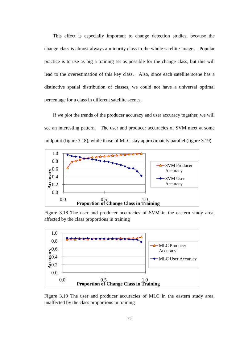
75
This effect is especially important to change detection studies, because the
change class is almost always a minority class in the whole satellite image. Popular
practice is to use as big a training set as possible for the change class, but this will
lead to the overestimation of this key class. Also, since each satellite scene has a
distinctive spatial distribution of classes, we could not have a universal optimal
percentage for a class in different satellite scenes.
If we plot the trends of the producer accuracy and user accuracy together, we will
see an interesting pattern. The user and producer accuracies of SVM meet at some
midpoint (figure 3.18), while those of MLC stay approximately parallel (figure 3.19).
Figure 3.18 The user and producer accuracies of SVM in the eastern study area, affected by the class proportions in training
Figure 3.19 The user and producer accuracies of MLC in the eastern study area, unaffected by the class proportions in training
0.0
0.2
0.4
0.6
0.8
1.0
0.0 0.5 1.0
Acc
urac
y
Proportion of Change Class in Training
SVM Producer Accuracy
SVM User Accuracy
0.0
0.2
0.4
0.6
0.8
1.0
0.0 0.5 1.0
Acc
urac
y
Proportion of Change Class in Training
MLC Producer Accuracy
MLC User Accuracy

This implies that, the omission
machine learning algorithms are determined in the training stage, directly related to
the amount of training pixels in each class. The maximum likelihood algorithm
though now often considered inferior by the community,
The trends in the figures of user accuracy and producer accuracy give the overall
picture of this issue. We will also give a more visual examination of the spatial
patterns compared against the ground reference map. This should indicate the
locations of overestimation and underestimation errors. We would also like to find
out whether overestimation
We will show the results from different algorithms and training proportions side
by side in a representative sub
difficult one for change detection among the three test
phenology between the two image dates. It also has the inter
phenomenon on the nonforest land surface between the two image dates. The
following figures show the Landsat TM 7
composite image, and the forest change reference map.
Figure 3.20 Landsat TM 7(Right)
76
This implies that, the omission and commission rates of the powerful new
machine learning algorithms are determined in the training stage, directly related to
amount of training pixels in each class. The maximum likelihood algorithm
though now often considered inferior by the community, is largely unaffected.
The trends in the figures of user accuracy and producer accuracy give the overall
sue. We will also give a more visual examination of the spatial
patterns compared against the ground reference map. This should indicate the
locations of overestimation and underestimation errors. We would also like to find
out whether overestimation and underestimation are solvable by post
We will show the results from different algorithms and training proportions side
by side in a representative sub-region of the west test area. This test
difficult one for change detection among the three test areas. It has a varied forest
phenology between the two image dates. It also has the inter
phenomenon on the nonforest land surface between the two image dates. The
owing figures show the Landsat TM 7-4-2 composite image, Landsat ETM+ 7
composite image, and the forest change reference map.
Landsat TM 7-4-2 (Left), ETM+ 7-4-2 (Center), Change reference
commission rates of the powerful new
machine learning algorithms are determined in the training stage, directly related to
amount of training pixels in each class. The maximum likelihood algorithm,
is largely unaffected.
The trends in the figures of user accuracy and producer accuracy give the overall
sue. We will also give a more visual examination of the spatial
patterns compared against the ground reference map. This should indicate the
locations of overestimation and underestimation errors. We would also like to find
post-processing
We will show the results from different algorithms and training proportions side
. This test area is the most
. It has a varied forest
phenology between the two image dates. It also has the inter-annual flooding
phenomenon on the nonforest land surface between the two image dates. The
2 composite image, Landsat ETM+ 7-4-2
2 (Center), Change reference map

We have 342 classification results in total and thus could not show all of them
here. Instead, we will only show 18 classification results, in which six algorithms
are fed with three types of training sets. The first training set has 5% data
forest change. The second training set has 50% data labeled as forest change. The
third training set has 95% data labeled as forest change.
Figures 3.21 to figure 3.26 illustrates how different supervised classifiers handle
training sets of same amount yet different class proportions.
Figure 3.21MLC Classification with 5% change training (Left), with 50% change training (Center), with 95% change training (Right)
Figure 3.22 DT Classification with 5% change training (Left), with 50% change training (Center), with 95% change training (Right)
77
We have 342 classification results in total and thus could not show all of them
Instead, we will only show 18 classification results, in which six algorithms
are fed with three types of training sets. The first training set has 5% data
forest change. The second training set has 50% data labeled as forest change. The
third training set has 95% data labeled as forest change.
Figures 3.21 to figure 3.26 illustrates how different supervised classifiers handle
ame amount yet different class proportions.
MLC Classification with 5% change training (Left), with 50% change training (Center), with 95% change training (Right)
DT Classification with 5% change training (Left), with 50% change training (Center), with 95% change training (Right)
We have 342 classification results in total and thus could not show all of them
Instead, we will only show 18 classification results, in which six algorithms
are fed with three types of training sets. The first training set has 5% data labeled as
forest change. The second training set has 50% data labeled as forest change. The
Figures 3.21 to figure 3.26 illustrates how different supervised classifiers handle
MLC Classification with 5% change training (Left), with 50% change
DT Classification with 5% change training (Left), with 50% change

Figure 3.23 SVM Classification with 5% change training (Center), with 95% change training (Right)
Figure 3.24 KP Classification with 5% change training (Left), with 50% change training (Center), with 95% change traini
Figure 3.25 ARTMAP Classification with 5% change training (Left), with 50% change training (Center), with 95% change training (Right)
Figure 3.26 SOM Classification with 5% change training (Left), with 50% change training (Center), with 95% change training (Right)
We have observed that,
78
SVM Classification with 5% change training (Left), with 50% change training (Center), with 95% change training (Right)
KP Classification with 5% change training (Left), with 50% change training (Center), with 95% change training (Right)
ARTMAP Classification with 5% change training (Left), with 50% change training (Center), with 95% change training (Right)
SOM Classification with 5% change training (Left), with 50% change training (Center), with 95% change training (Right)
We have observed that, when the class proportions in the training set vary
training (Left), with 50% change
KP Classification with 5% change training (Left), with 50% change
ARTMAP Classification with 5% change training (Left), with 50%
SOM Classification with 5% change training (Left), with 50% change
when the class proportions in the training set vary, the

79
Maximum Likelihood Classifier is much more robust than the newer and more
popular classifiers. SVM has shown desirable properties consistently in previous
experiments, but this experiment identified that SVM shares the same problem with
neural nets and decision tree in this aspect. The quality of classification results can
be very bad if the proportions of training classes are left to be arbitary. This is a
serious source of error.
We also found that, when the producer accuracy curve meets the user accuracy,
the percentage of the forest change pixels in the training data is somewhat but not
strictly related to the percentage of the forest change pixels in the whole study area.
The following table illustrates this vague relationship.
Table 3.7 Percentage of Forest Change pixels in training data when optimal SVM performances are achieved
Study Area Percentage of Forest Change
pixels in study area
Percentage of Forest Change pixels in
training data with optimal performance
Atlantic Forest 24.8% 25%
Humid Chaco 8.4% 15%
Dry Chaco 7.2% 10%
These numbers give us some hopes. Maybe, to achieve the optimal accuracy,
SVM has to have a carefully-selected training data set that has the same class
proportions as the data population? However, the data population is not known
before the change detection. How can we solve this ‘chicken-and-egg’ dilemma?
Let us continue with the experiments, and return to this question in the summary
section of this chapter.

80
3.8. Assessing the Algorithms with Scarce Training Data
Traditional assessments of change detection algorithms are usually based on
ample training data. But it is not practical to always have ample training data
collected from field trips and high-resolution photo interpretation everywhere on
Earth. A good algorithm needs to be able to achieve reasonably good accuracy when
the available training data is scarce.
Algorithms need to cope with scarce training data not just because the total
training data might be scarce. If one class only has a small amount of training data
while the other classes have disproportional ample training data, our experiment in
section 4.7 have demonstrated the effect. Accuracy decreases sharply when the
training data sampling does not comply with the Equal Sample Size (ESS) rule.
Therefore, any class with scarce training data will lead to the reduction of total
number of training pixels. Thus it is vital that algorithms for large-area forest
change detection must perform well with less-than-perfect amount of training data.
This experiment was also conceived in the very early stage of this dissertation, and
only SVM and Decision Tree were tested.
Our experiment in this section assesses the accuracies using different amount of
training data. For the Atlantic Forest study area, which has roughly 10 million pixels,
the result is listed in table 3.8.
Our experiment shows that, SVM and DT do not need a lot of training pixels to
achieve good accuracy. And when they use the same amount of training data, SVM

81
consistently out-performs DT. We can also interpret the finding in another direction:
There is an intriguing limit of classification accuracy irrelevant to training size.
Table 3.8 The effect of training data scarcity on accuracy
Training pixel Count SVM Overall Accuracy DT Overall accuracy
12500 0.8823 0.8510
10000 0.8790 0.8433
7500 0.8774 0.8473
5000 0.8833 0.8465
2500 0.8785 0.8454
In the Ph.D Dissertation of Dr. Chengquan Huang (Huang 1999), he also looked
at this aspect. His observation was that the SVM algorithm at that time needs a
training set 6% of the total data volume. It now seems that his evaluation might be
conservative. Apparently, the SVM algorithm does not lose much accuracy even
when the training set is less than one thousandth of the data population.
3.9. The Algorithm of Best Overall Performance
Our empirical cross-comparison of change detection algorithms aims at
comparing the detection power of algorithms on a fair basis, and compare them as
close to real-world situations as possible so as to challenge them with uncertainties.
The influences of less-than-perfect training data are well considered, in order to find
algorithms that are truly robust and accurate.
Our assessment in section 3.3 show that geographical variations do have impact
on the accuracy of all the algorithms, but SVM and Kernel Perceptron consistently
excel. Our experiment in section 3.4 shows that SVM, Kernel Perceptron, and
Decision Tree all have good capabilities in handling large-area variation. Our

82
experiment in section 3.5 shows that SVM and Kernel Perceptron have outstanding
error tolerance. Our experiment in section 3.6 shows that SVM is not significantly
impacted by training data located in the transitional land cover. Our experiment in
section 3.7 shows that the modern algorithms are heavily affected by the sampling
method of the training data while the old-school MLC is almost not affected. Our
experiment in 3.8 shows that both SVM and Decision Tree can work with
less-than-conventional amount of training data and still get good results.
When these results are linked with the theoretical strengths and limitation
outlined in chapter 2, we can see that some of the theoretical characteristics are
verified, while some are rejected.
SVM and KP do have the theoretical advantages of handling geographical
variations and high error-tolerance. SVM does not have the theoretical disadvantage
of the Gaussian assumption as MLC has, because the Gaussian kernel in SVM is the
more versatile multi-modal Gaussian distribution. However, the generalization
power of KP is not as good as that of SVM.
We conclude that, the machine learning community has already built an excellent
baseline classifier for us. The SVM family can tackle most types of known
uncertainties and errors in remote sensing applications. It is much better than
Decision Tree and Neural Nets. To be specific, when >85% of the training data is
reliable, Kernel Perceptron is the best algorithm to perform forest change detection.
When <85% of the training data is reliable, then the standard SVM with RBF kernel
is the solution. However, in real-world applications, it is often difficult to know a

83
priori the percentage of errors in our observations. Therefore, it is safer to use the
SVM with RBF kernel as a baseline algorithm.
Table 3.9 The theoretical strengths and suspected weaknesses revisited
Algorithm Family Algorithm
Name
Validated Strengths Validated Weaknesses
Bayes Classifiers MLC N/A Lower accuracy in
complicated,
high-dimensional features
No error tolerance
Entropy-minimization DT Good accuracy in
large-scale studies
Salt-and-pepper errors
Mediocre error tolerance
Neural Networks ARTMAP Training pattern can be
improved with incoming
data for classification
In developing and varies a
lot among versions
Margin-maximization SVM High accuracy at all scales
High error tolerance
sampling bias can hurt
Kernel KP High accuracy at all scale
Medium error tolerance
Boosting without extra
computational time
sampling bias can hurt
Meanwhile, we discovered an unreported source of error for most of the
contemporary machine learning algorithms. The relative proportions of classes in
the training set exert a powerful hidden influence on the classification results. It is
unlikely that any remote sensing study can construct a perfect training set by chance.
We must understand where this error source originates from, and how to bring it under
control. This effort will be outline in the next two chapters.

84
4. Optimizing Class Proportions in the Training Set
4.1. Class Proportions in Training Data: an Overlooked Pitfall
In chapter three we have discovered that, the performance of most supervised
classifiers are significantly affected by the proportions of training data used to
represent each class. Change detection studies are particularly heavily affected by
this side effect, given that the change classes are quite unique. The change class is
numerically a minority class in most studies. The number of change pixels is often
highly variable from one satellite scene to another. The change classes are also often
of highest importance. Therefore, the proportions of the change classes are small,
variable, and important. This fact makes them the most susceptible classes under the
newly discovered pitfall.
How do we quantify the severity of this pitfall? In remote sensing studies, the
producer accuracy is defined as the detection success against omission error, and the
user accuracy is defined as the detection success against commission error (Congalton
1991). In section 3.7, we studied empirically the dynamic nature of producer
accuracy and user accuracy as they are influenced by class proportions in training.
They seem able to catch the problem. How serious is it?
For the case of Decision Tree, when the proportion of change class in the training
set is gradually adjusted from 5% to 95%, the producer accuracy increases from 64%

85
to 98% while the user accuracy drops from 95% to 45%. In addition to Decision
Trees, other popular contemporary algorithms such as Support Vector Machine,
ARTMAP neural nets, and Self-organizing Maps also fall prey to this pitfall. The
only algorithm that is largely immune to this effect is the Maximum Likelihood
Classifier. The user and producer accuracy produced by MLC are invariant,
although not always unbiased, when the class proportions in the training data change.
Therefore, we interpret our empirical findings as: most nonparametric classifiers
increasingly overestimate any class when the training data proportion of that class
increases in a training set of fixed size. Vice versa, they increasingly underestimate
any class when the training data proportion of that class decreases in a training set of
fixed size. In short, the outcome of classification is highly dependent on the class
proportions in training.
There seems to be a simple internal relationship between underestimation and
overestimation in classifiers. This relationship can be easily pushed in any direction
by increasing or decreasing training data in a class. Therefore, this issue likely does
not just exist in change detection studies, but also is present everywhere in the broader
field of classification of remotely sensed data.
Through our empirical study in chapter three, we have found that, different
geographical regions have different patterns of overestimation and underestimation.
This implies that a significant challenge exists in continental-to-global classification
study of remotely sensed data. If we have little or no control over the balance of
underestimation and overestimation errors, then the same class might be

86
underestimated in one satellite scene yet overestimated in another. In addition, the
smaller the satellite footprint is, the more likely it is affected.
This effect was well hidden in a sense. In chapter three, we found that when the
proportion of change class in the training set was adjusted from 5% to 80%, the
overall accuracy always stays above 85%, which is a decent performance. In most
real-world applications, the overall accuracies are often used as a benchmark for
project success. The overall accuracy hides the variations in user and producer
accuracies. In remote sensing studies, researchers are often interested in thematic
information of one class, such as forest, water, and urban, instead of all the classes.
Those studies will suffer the most from this pitfall. Change detection studies are
also among the most-affected because a single change class such as deforestation is of
highest importance, yet the problem has been hidden.
The sufficiency of training is not a new topic of discussion. In the past,
researchers have directed their attentions to the sufficient quantity of training.
Several contemporary studies have looked at the effect of the total training set (Foody
et al. 1995; Foody and Mathur 2004; Song et al. 2005; Foody et al. 2006; Rogan et al.
2008), and the effect of sufficient training data for each class (Pal and Mather 2003),
but there has been no study of over- and under-estimation caused by class proportions
in the training set.
In this chapter, we will investigate the mathematical origin, magnitude of impact,
and the solution to this newly-found pitfall that greatly challenges the reliability of
data products from remote sensing.

87
4.2. Why are Modern Classifiers Heavily Influenced by Class
Proportions in the Training Data?
Modern supervised classification of remotely sensed data starts with a training
dataset usually collected either through fieldwork, or visually-interpreted
high-resolution images. The training process effectively tunes the classifier model
towards the best overall accuracy for a given training set. The tuned classifier model
is then applied to the whole image. The classification result is then compared to a
set of and reference validation data for accuracy assessment. The accuracy
assessment benchmarks the performance of the classification, and gives a confidence
interval of accuracy on the whole image. Very often, the training data and the
validation data come from the same fieldwork or image interpretation process.
This has been a quite standard procedure for the past three decades. Past studies
on the general methodology of training procedures have focused on two topics:
1. How to collect training data so that the training data covers all the features in
the feature space while being minimal in numbers (Foody and Mathur 2004; Foody et
al. 2006).
2. How to choose the sampling scheme for validation dataset in accuracy
assessment so that we can estimate the confidence interval for accuracy on the whole
classified image (Stehman et al. 2003; Stehman 2005; Stehman et al. 2009).
An overlooked aspect is the arrangement of class balance inside the training set.
Collecting training data in real-world applications is costly and often limited by

88
geographical accessibility.
We propose that, the sampling design of the training set should not be based on
data availability, or merely for the convenience in statistical accuracy estimation, but
instead it should be directly targeted for the optimization of a given classifier
algorithm.
In chapter three we demonstrated that the supervised classification process is
more complicated than simply building classification models based on an arbitrary
training dataset available. In this section, we will examine, one by one, how modern
supervised classifiers were designed to use the class information of the training data.
4.2.1. Maximum Likelihood Classification
The training process of MLC is solely dependent on two basic statistical
measurements: the mean of each class, and the covariance matrix among all the
classes (Equation 2.6). These two form an ellipsoid for each class in the feature
space. If we introduce more training data points only for one class, the mean and
covariance matrix are not easily changed. MLC uses the covariance matrix in the
determination of class boundaries. Thus the class boundaries are not easily
changeable and the classification result is also not easy to be changed.
However, when a class is described by only a very small amount of training data,
and that small training set contains some errors due for example to misregistration or
misinterpretation of ground features, then the mean center of the class might be
substantially changed. This could explain the sudden drop of accuracy at extreme

89
ends in graphs in section 3.7
Another known problem regarding classes happens when the ellipsoids
characterizing different classes are not separable. They can simply overlap with
each other, or go through one another. In that case, MLC might fail completely.
This is caused by the definition of classes, not caused by class proportions in training.
4.2.2. Decision Trees
The training process of DT starts with calculating Entropy of the training dataset.
∑=
−=n
iii ppSEntropy
1
)ln()( (Equation 4.1)
In this equation, pi is the percentage of data points in class i out of the whole
training set. It is very obvious that if we introduce more training points into one of
the classes, the calculation of Entropy is now significantly affected. Thus the
building of the decision tree will be altered. Therefore, Decision tree might be the
classifier most sensitive to class proportion variations in the training set.
4.2.3. ARTMAP Neural net
The training process of ARTMAP is the matching process of clusters identified by
two ART modules. One ART module performs clustering using the training label,
and the other ART module performs clustering using the spectral data. Increasing
the amount of training data for an arbitrary class would increase the ‘coverage’ of
clusters of that class in the feature space, and leads to overestimation. However,
judging from this mechanism, the center of the clusters should not be changed a lot.

90
ARTMAP is expected to be less sensitive to the variation of training data proportions
than Decision Trees.
4.2.4. Support Vector Machine and Kernel Perceptron
The contemporary SVM and KP algorithms are based on the soft-margin SVM
design. The internal optimization function is ))(2
1(min
1∑=
+>•<p
kk
wCFww ξ , in
which C is the penalty coefficient and kξ varies between 0-1, allowing some data
points to exist between the hyperplanes (class boundaries) in Hilbert Space. This
design was first introduced to effectively deal with inseparable classes. In chapter
three, we found that it also had an unplanned but useful side-effect of error tolerance.
However, this design also leads to another unplanned and unwanted side-effect: the
hyperplanes could be pushed to move substantially. When a class is given more
training data, the hyperplanes around this class will be pushed outwards, eroding other
classes. This might be one origin of the problem.
Another hidden mechanism is the cross-validation (CV) stage (Stone 1974) in the
tuning of classifiers. SVM with a specific kernel needs to tune the parameters of the
kernel for the maximum possible accuracy. This CV stage can achieve best accuracy
for a given training set. However, there has been no documented rule on how to
construct the training set for CV. Researchers usually just take a random sub-sample
of the available training data. This also might be another cause of the problem.
Worth noticing is that, this dubious CV process is also present in most neural nets.

91
4.2.5. Self-Organizing Maps coupled with Learning Vector Quantization
(SOM-LVQ)
Kohonen’s Self-Organizing Map (SOM) neural network is a special kind of
neural network. It is not a typical feed-forward network, and not a typical recurrent
network. It does not have the popular design of hidden layers either. It consists of
two layers: the input layer which contains neurons of the amount of input data
dimension, and the output layer which contains a two-dimensional neuron array.
Figure 4.1 The workflow of Self-Organizing Maps (Cited from the help file of the Idrisi software)
In the first step of training stage, known as the ‘coarse tuning’, the neurons in the
output layer are derived in such a way that the neurons corresponds to clusters in the
spectral data, and each neuron is kept at a distance from other neurons. Neurons are
then labeled into each class.
In the second step of training stage, known as the ‘fine tuning’, Learning Vector
Quantization (SOM-LVQ) creates a topology of neurons in the output layer.
Neurons that are similar in the feature space will make the class boundary expanding
outward.

92
The design of SOM-LVQ is somewhat controversial for the issue of class
proportions in training data. The ‘course tuning’ part will not provide a very high
accuracy in the training area, but might be effective against the pitfall
overestimation-underestimation. The ‘fine tuning’ part will provide a high accuracy
in the training area, but is susceptible to the pitfall of overestimation-underestimation.
In summary, SOM might be of some value without the ‘fine tuning’ phase, but it is to
be examined in real-world cases. SOM-LVQ was discussed only briefly in chapter
two. It was not used in chapter three. It is introduced here simply because of its
potential to help overcome the pitfall of over and underestimation.
4.3. Prioritized Training Proportions (PTP): Reducing the
uncertainties in classification and change detection of satellite data
In the previous discussion, we have outlined the uncertainties and the possible
causes of a previously hidden issue for all classification-based change detections.
Empirical studies in chapter three showed that all modern supervised classifiers but
MLC are strongly affected by variations in training set proportions, and that past
studies in the methodology of machine learning have not identified this issue yet.
Remote sensing studies, especially those aiming at continental-to-global scales,
need a way to minimize this uncertainty. In this section, two candidate solutions are
proposed by going to the source mechanisms of supervised classifiers, and by
combining the strengths of different hard classifiers to make a joint classifier. This
is expected to reduce the uncertainties in the overestimation-underestimation dilemma.

93
This joint classifier will be based on a new optimization goal, and make use of SVM
and MLC together.
4.3.1. A Tale of Two Optimization Rules
With the exception of MLC, all modern supervised classifiers described
previously have the same optimization rule: maximization of overall accuracy in the
dataset used for cross validation. The dataset used for cross validation, however, is
usually only a random subset of the training set. Thus Bayes Optimal was aimed for
the data population but actually achieved for the sample. Therefore, the first
optimization rule we propose, is to indeed achieve Bayes Optimal for the data
population.
Another optimization rule we propose here is the minimization of the absolute
difference between the estimated omission data points and commission data points for
a Key class. Let us call this the Bayes Optimal for a Key Class.
Assume there are M classes in the dataset, and the proportion of each class in the
training set is written as KP , i=1 …, K,… M. The Kth class is chosen as the most
important class.
11
=∑=
M
iiP
, 1<K≤ M
The proposed optimization rule is to feed a supervised classifier with training
datasets designed to have KP enumerated from 0~1, and find out the optimal KP so
that:

94
||min CK
OK
P
NNArgK
− (Equation 4.2)
where OKN is the pixel count of Omission errors in the K(ey) class, and C
KN is
the pixel count of Commission errors in the K(ey) class.
OKN and C
KN are the direct results of a chosen scenario of class proportions in a
training dataset with a fixed total amount of data points.
This optimization rule defines the optimal classification as when the magnitude of
omission errors is closest to that of commission errors for the Key class. It is
designed this way because in the general classification applications, not all the classes
are of equal importance. Especially in change detection applications, the change
class is always of the highest importance. The optimization rule prioritizes the Key
class, and thus we call it PTP (Prioritized Training Proportions).
Geographers are more familiar with the confusion matrix. Let us use it to
illustrate our ideas. For a 3-class classification of Persistent Forest, Persistent
Nonforest, and Forest Change, we have the following confusion matrix:
Table 4.1 A standard confusion matrix for a 3-class classification
Classification
Assessment Persistent Forest Persistent Nonforest Forest Change
Persistent Forest A1 A2 A3
Persistent Nonforest B1 B2 B3
Forest Change C1 C2 C3
The Bayes Optimal for the data population goal maximizes the sum of the
diagonal items (A1+B2+C3).
The Bayes Optimal for a Key Class goal, when we treat the Forest Change class
as the key class, minimizes the absolute difference in [(A3+B3) - (C1+C2)]

95
Another perspective to interpret the Bayes Optimal for a Key Class goal is rather
important in reality. For example, a carbon model needs an unbiased estimation of
the forest change inventory statistics in the Amazon, but it does not need a quality
map. The total amount of forest change found by the classifier is A3+B3+C3, while
the total amount of forest change found by the assessment is C1+C2+C3. The
carbon model wants these two numbers to be as close as possible, which means the
minimization of the absolute difference in [(A3+B3+C3)_- (C+C1+C2)], which is
equal to [(A3+B3) - (C1+C2)]. This is the Bayes Optimal for a Key Class goal.
Other researchers have already outlined similar goals, just without a working
solution. In R. M. Lark’s milestone paper (Lark 1995) he listed a large number of
possible optimization goals, and this was listed as his goal No. B1. He tried to give a
solution using prior probability modeling in the MLC framework. We will discuss
more in the next chapter and show why the solution is wrong. The so-called ‘Pareto
Boundary’ of omission-commission errors (Boschetti et al. 2004) is basically the same
thing but with an unnecessarily complicated mathematical model, which gives an
ambiguous zone of possible solution. Another study also concentrated on this
question and tried to extend Lark’s work. It was identified (Boyd et al. 2006) that
‘statistically significantly increases in accuracy were achieved through the use of
simple binary classifications by DT and SVM that aimed to separate the class of
interest from all others.’ But how this worked was not understood.
These two optimization rules are actually very straightforward both in theory and
in implementation. It only takes three simple steps to implement them.

96
The first step is to construct a cross validation dataset maxV using a subset of all
the available training data. This validation dataset will have approximately the same
class proportions as in the whole study area. These class proportions should be
estimated without full prior knowledge of the data population. In the next section
we will discuss in details how to do this. Both optimization rules will need this step,
but only the PTP rule needs the next two steps.
The second step is to create many training datasets using the available training
data points. These different training datasets will be denoted as KiT because they
enumerate all the possible KP values from 0 to 1. These different training datasets
will be used to train classifiers and find out which training dataset produces
||min CK
OK
P
NNArgK
− . The optimal KP is denoted as *KP .
The third step is to create the largest possible training dataset *KT with the
optimal *KP . This training dataset will be used to build the optimal classifier that is
used for the change detection analysis.
These three steps will be discussed in details subsequently in three subsections.
4.3.2. Redefining Cross Validation
Contemporary supervised classification algorithms seek the maximization of
overall accuracy in cross validation (CV). For example, the RBF kernel used in
SVM requires the parameters C and gamma (explained in section 4.2.4) that produces
the best overall accuracy. Contemporary cross validation is the so-called “N-fold
Cross Validation” (Stone 1974), in which all the available training data points are

97
evenly partitioned into complementary subsets, performing the analysis on one subset
(called the training set), and validating the analysis on the other subset (called the
validation set or testing set). This CV approach uses a validation set with
approximately the same class proportions as in the training set. This is, however, a
hidden link between the training set and the validation set.
The validation set used in our algorithm must have the same class proportions of
the whole study area. In this way, cross validation will generate the optimal
parameter set not just for the validation set, but also for the whole population.
However, before the change detection, we do not know the true class proportions in
the whole study area. Even after conventional supervised change detection, the
estimated class proportions in the whole study area are not reliable because of the
overestimation-underestimation problem among the classes. This is a
chicken-and-egg dilemma.
Fortunately, we discovered in chapter three that MLC has the rare property of
being largely resistant to the overestimation-underestimation problem among the
classes. Thus we can perform an initial round of change detection using MLC with a
training set with equal amount of training data in each class. This does not give us a
classification result of fabulous quality, but it gives us an unbiased estimation of the
class proportions in the whole data population. This information is called “class
prior” in hundreds of papers published from 1980s to 1990s (Strahler 1980; Lark
1995). We will discuss more about it in section 4.5.5. Those studies use this “class
prior” information in the posterior probability modeling of classification results. In

98
Lark’s study, he outlined different classification optimization goals, and varied the
class prior probability among the classes to achieve those goals. Our approach, on
the other hand, varies the class proportions in the training and validation sets.
Let us use a concrete example to illustrate how to create a standardized validation
set. Assume that we are studying three classes in a study area of 500 square
kilometers. We have 1000 known data points available. 500 data points belong to
class A, 410 points belong to class B, and 90 points belong to class C. Class C is the
key class, i.e. the class of highest practical importance. We will perform a MLC
change detection using 90 training points in each class. Then we find out the
approximate class proportions in the study area are: 55%, 32%, and 13%. Then we
retrieve the largest possible subset within this set of 1000 points: maxV =min(500/0.55,
410/0.32,90/0.13)=692, of which 380 points comes from class A, 221 points come
from class B, and 90 points come from class C.
4.3.3. Enumeration of Key Class Proportion in the Training Dataset
After we have a standardized validation set, we will use it to find what the
optimal class proportions in the training set really are. The goal is to achieve the
minimization of difference between commission error and omission error for a given
key class. This is performed through the enumeration of key class proportion in the
training set.
Let us use a concrete example to lay out this idea. Assume we have 1000 data
points collected from the study area. Three classes (A, B, and C) are used in the

99
study. The enumeration of class proportions will be shown in table 4.2:
Table 4.2 An example for enumeration of key class proportion in training data
Enumeration of Key
Class Proportion ( )
Percentage of training
points in class C
Percentage of training
points in class B
Percentage of training
points in class A
10% 10 45 45
20% 20 40 40
30% 30 35 35
40% 40 30 30
50% 50 25 25
60% 60 20 20
70% 70 15 15
80% 80 10 10
90% 90 5 5
Although we have 1000 ground data points available, we do not use all of them
together. In the enumeration of key class proportion, we need to make sure the total
number of training points stays invariant. In other words, we want to isolate the
effect of class proportions from the effect of training dataset size.
Each training set is used to construct a classification model, and is then applied to
the standardized validation set maxV . Omission error ( OKN ) and commission error
( CKN ) are then calculated. Table 4.3 shows the detailed procedure for optimization.
In this table, we find that the balance between commission error and omission
error is reached somewhere when KP is between 10% and 30%. We repeat this
step using finer stepping of 1% increment in the range of 10% and 30% to seek for the
optimal balance point *KP . For example, we might find it at 17%.
KP

100
Table 4.3 An illustration of possible omission-commission dynamics due to enumeration of key class proportion in the training set
Enumeration of Key
Class Proportion ( )
Commission error in
key class ( )
Omission error in
key class ( )
10% 0 45 45
20% 2 10 8
30% 10 0 10
40% 17 0 17
50% 50 0 50
60% 120 0 120
70% 340 0 340
80% 560 0 560
90% 650 0 650
4.3.4. Constructing the Largest Possible Training Dataset and the Optimal
Classifier Model
With the optimal balance point *KP located for the key class, we will construct
the largest possible training dataset *KT out of the 1000 available data points. It is
min(550/((1-0.17)/2),410/((1-0.17)/2),90/0.17)=529, of which 220 points come from
class A, 220 points come from class B, and 89 points come from class C. In this
training set *KT , every class that is not the key class shares equal amount of training
points. Strictly speaking, this is still not the ideal solution for the non-vital classes.
An improvement would be to rank the class in order of importance, and optimize
them class after class recursively. However, this idea is left for future development.
*KT is then used to derive the best classifier model. In doing so, it is very
important that we need to bypass the cross validation built in those classifiers. The
reason is that we already achieve a better cross validation described in 4.3.2 and 4.3.3.
If we allow the classifiers to use the built-in CV procedure, it would not be optimal.
KP CKN O
KN|| C
KOK NN −

101
However, the classifiers still need some parameters, such as C and gamma in the
case of SVM with RBF kernel. These are usually derived through CV. When we
bypass the CV procedure in the final training stage, we can directly use those
parameters derived in the process of identifying *KP .
With these three steps, we have improved the contemporary cross validation
notion in the field of machine learning, and we can build a joint classifier by linking
MLC to any classifier of SVM, DT, or ARTMAP neural nets. In chapter three we
have identified that SVM and KP have some unique strengths compared to others, and
thus the soft-classifier is implemented in this dissertation in the form of MLC-SVM.
In the next section, we will illustrate the performance of the joint classifier
MLC-SVM constructed using the method described in this section.
4.4. Assessment of the Joint Classifier MLC-SVM
4.4.1. Assessment Design
In this section, we will assess the practical use of two new approaches against a
widely-used contemporary practice, which consists of stratified sampling of training
data. The first new approach is to gain true Bayes Optimal for the whole data
population, and the second new approach is to gain Bayes Optimal for a key class in
the whole data population. These two goals were discussed in section 4.3.1.
The data we used in this assessment consist of eight neighboring Landsat
scene-pairs in Paraguay and also the corresponding forest change map. These scenes

102
contain very different deforestation patterns. In some scenes, about 20% of the total
land area was deforested in the time span of 10 years, whereas in other scenes, only
2%-3% of the total land area was deforested. We anticipated that, the variation of
class proportions in different areas will cause some variations in accuracy. This
offers us a good opportunity to study the different response of the three approaches.
In every Landsat scene, only the central 100km-by-100km region will be used.
This is a carefully calculated region ensuring no overlap with neighboring Landsat
scenes. This criterion for data selection will prevent unnecessary confusion due to
some areas being included twice.
For every Landsat scene, 2000 points collected from the forest change map are
assumed to be accurate and used as the training data. The methods of sampling o
will be described in the next section. The map of the whole 100km square
(3200-by-3200 pixel region) is used in the accuracy assessment after the change
detection.
Similar to the experiments in chapter two and three, we define three classes in
this multi-temporal assessment. They are forest-to-forest, nonforest-to-nonforest,
and forest change. Among the, the class of forest change is of highest importance
and is treated as the key class. There has been no noticeable land cover change of
nonforest-to-forest in the region. Thus we do not have this class in the experiments.
4.4.2. Approaches in Comparison
Three approaches are designed, with significant differences in the training stage.

103
The first one, namely the ‘Stratified’ approach, is the most popular approach used in
contemporary and past studies on remotely-sensed imagery and other machine
learning applications alike. The training set of 2000 points is chosen with equal
amounts from three classes. This is a stratified random sampling.
The second approach, namely ‘PTP’ approach, was described in section 4.3.1.
The training set of 2000 points is chosen with the optimal class proportions identified
as:
||min C
KOK
P
NNArgK
−. (Equation 4.2)
The technical steps were discussed in 4.3.2~4.3.4.
The third approach, namely the ‘Adaptive approach, is the simpler optimization
rule of the two discussed in section 4.3.1. It is very similar to the PTP approach, but
much simpler. Basically we construct the training and the validation sets with the
class proportions estimated using MLC. It needs the technical steps of 4.3.2, but not
the steps in 4.3.3 and 4.3.4. For its simple construction, we call it ‘Adaptive’.
Let us visualize how the modern classifiers work. With given classes A, B, and
C, the classifier tries to delineate the boundary among them. As we pointed out in
this chapter, the configuration of class proportions in the training data is the hidden
driving force behind the delineation of class boundaries. In the following drawing
(Figure 4.2), the three vertices are the centers of classes A, B, and C and the red dot is
the ideal place where the class boundaries should meet. The green lines meet at the
location where the class boundaries meet together.

104
Figure 4.2 Class boundary illustrations in three approaches
The “Stratified” approach uses the same amount of training data from each class,
and thus will overestimate the classes whose true proportion in the study area is less
than 1/3, and will underestimate the classes whose true proportion in the study area is
more than 1/3.
The “PTP” approach optimizes to find the optimal location for key class C, but in
the current version of PTP algorithm, we have no optimization between classes A and
B. Therefore, our solution is close to the ideal location, but not perfect.
The “Adaptive” approach uses the same proportions of training data as in the
whole study area, and thus should be quite close to the ideal solution of class
separation. However, the optimization rule in this scenario is the maximization of
overall accuracy, not emphasizing the key class. In studies with more classes, the
class boundary in the feature space will be more complicated. This adaptive
approach might be less effective in studies involving more classes.
In the next section, we will present the outcome of these three approaches. The
actual pictorial outcome will be also illustrated to show the obvious effect of
underestimation-overestimation.

105
4.4.3. Outcomes
The following table shows the overall accuracy of the eight Landsat scenes under
three different approaches. We can see that, there is really not much difference
between the “Stratified” approach and the “PTP” approach. But there is a significant
increase of accuracy from the “Stratified” approach and the “Adaptive” approach.
Table 4.4 Overall accuracy in 8 study areas of 3 approaches
Study Area (WRS-2
Path/Row)
Overall Accuracy in
“Stratified” approach
Overall Accuracy in
“PTP” approach
Overall Accuracy in
“Adaptive” approach
Area 1 (225/77) 89.8 89.7 91.2
Area 2 (225/78) 88.5 89.7 93.6
Area 3 (226/76) 87.5 89.6 92.4
Area 4 (226/77) 87.3 91 96.0
Area 5 (227/75) 91.9 93.4 94.1
Area 6 (227/76) 87.6 88.8 89.6
Area 7 (228/75) 85.6 86.4 Failed
Area 8 (228/76) 89.6 90.4 89.6
These results are better illustrated in the following chart.
Figure 4.3 Overall accuracy in eight study areas of three approaches
0102030405060708090
100
Area 1 Area 2 Area 3 Area 4 Area 5 Area 6 Area 7 Area 8
Accuracy
Overall Accuracy with the Stratified Training Set Overall Accuracy with the Adaptive Training SetOverall Accuracy with the PTP Training Set

106
The “Adaptive” approach was designed because we anticipated it to have better
performance than the “Stratified” approach. It used the class proportions estimated
by MLC to construct a training set for SVM. The same step is used as the first step
in PTP algorithm.
What surprised us is that this adaptive approach seems to have even better
performance than the “PTP” approach, in which we did extra optimization on the key
class. There are two possible reasons for this unexpected finding. The first reason
is that this version of the PTP algorithm only optimizes one key class, while ignoring
the other two classes. The PTP algorithm should be further developed into a
recursive optimization of classes ranking from most important to least important.
Then it should outperform the adaptive approach. The second reason is that our
change detection is basically a 3-class supervised classification. We have illustrated
in the previous section that, such a simple case favors the adaptive approach. As the
number of classes increase, the class boundary in the feature space will be more
distant from the adaptive estimation. The recursive PTP approach might be more
successful at that time.
We also found that, the adaptive approach failed completely in test area seven. 7%
of the total land area in scene 7 is forest change, and the land cover patterns are very
complex. What happened in the adaptive approach is that, the class abstraction
power of MLC failed almost entirely to identify the change signal and estimated that
only 0.1% of the land area is forest change. The training set fed to the SVM
procedure thus only contains very few change pixels. Due to the soft-boundary

nature of SVM, the change class is completed ignored in the output. The resulting
change map carries no change at all, and is thus co
Let us also look at the user accuracy and producer accuracy of the most important
class: the forest change class. The following figures tell the real story hidden behind
the seemingly identical numbers of total accuracy in figure
Figure 4.4 The User Accuracies and Producer Accuracies after Stratified Training
We can see from Figure 4.4 that, user and producer accuracies are really unequal.
The difference between them can be huge in some
scenario, the producer accuracy is always much higher than the user accuracy. This
indicates gross overestimation of the change class. Why did it happen? In a
stratified 3-class supervised classification, training data from each class are of equal
amount. However, we know that the forest change class usually only take up a small
percentage, such as 1%~10% of the land surface. The change class is almost always
the minority class in any thematic change detection analysis. Therefore, assigning
equal amount of training data to each class almost always will lead to over
107
nature of SVM, the change class is completed ignored in the output. The resulting
change map carries no change at all, and is thus considered a total failure.
Let us also look at the user accuracy and producer accuracy of the most important
class: the forest change class. The following figures tell the real story hidden behind
the seemingly identical numbers of total accuracy in figure 4.3.
The User Accuracies and Producer Accuracies after Stratified Training
We can see from Figure 4.4 that, user and producer accuracies are really unequal.
The difference between them can be huge in some test areas. In the “Stratified”
scenario, the producer accuracy is always much higher than the user accuracy. This
s gross overestimation of the change class. Why did it happen? In a
class supervised classification, training data from each class are of equal
amount. However, we know that the forest change class usually only take up a small
ch as 1%~10% of the land surface. The change class is almost always
the minority class in any thematic change detection analysis. Therefore, assigning
equal amount of training data to each class almost always will lead to over
nature of SVM, the change class is completed ignored in the output. The resulting
nsidered a total failure.
Let us also look at the user accuracy and producer accuracy of the most important
class: the forest change class. The following figures tell the real story hidden behind
The User Accuracies and Producer Accuracies after Stratified Training
We can see from Figure 4.4 that, user and producer accuracies are really unequal.
. In the “Stratified”
scenario, the producer accuracy is always much higher than the user accuracy. This
s gross overestimation of the change class. Why did it happen? In a
class supervised classification, training data from each class are of equal
amount. However, we know that the forest change class usually only take up a small
ch as 1%~10% of the land surface. The change class is almost always
the minority class in any thematic change detection analysis. Therefore, assigning
equal amount of training data to each class almost always will lead to over-estimation.

Let us check if the PTP and Adaptive approaches can do the job better.
Figure 4.5 The User Accuracies and Producer Accuracies after PTP Training
The balance between user accuracy and producer accuracy is much better, but
some cases still far from ideal.
Figure 4.6 The User Accuracies and Producer Accuracies after Adaptive Training
The “PTP” scenario and “Adaptive” Scenario both lead to
producer accuracy and
108
the PTP and Adaptive approaches can do the job better.
The User Accuracies and Producer Accuracies after PTP Training
The balance between user accuracy and producer accuracy is much better, but
some cases still far from ideal.
The User Accuracies and Producer Accuracies after Adaptive Training
The “PTP” scenario and “Adaptive” Scenario both lead to
and user accuracy. In half of the areas (areas 2, 3, 4, 6), those two
the PTP and Adaptive approaches can do the job better.
The User Accuracies and Producer Accuracies after PTP Training
The balance between user accuracy and producer accuracy is much better, but in
The User Accuracies and Producer Accuracies after Adaptive Training
The “PTP” scenario and “Adaptive” Scenario both lead to more balanced
2, 3, 4, 6), those two

109
scenarios improved the user accuracy very significantly (20%~70%).
This shed light on one of the oldest mysteries of change detection: while the
overall accuracy is quite decent, why do we have very low user and producer
accuracies of the change class in some studies? Our answer is that, the hidden flaw
in the design of the training stage causes the poor user and producer accuracies in the
change class. This is completely avoidable.
Another purpose for the PTP algorithm is to give the closest estimation for the
total amount of the key class. This was discussed in section 4. 3.1. Did we achieve
that goal? Let us evaluate the ratio between the amount of change pixels detected
and the amount of change pixels in reality.
Table 4.5 The amount of detected change normalized by that of real change
Area (WRS-2
Path/Row)
Stratified Training PTP Training Adaptive Training
Area 1 1.27 1.15 1.05 Area 2 2.97 1.34 1.19 Area 3 2.63 1.45 1.03 Area 4 16.85 5.87 2.15 Area 5 1.23 1.02 1.00 Area 6 1.99 1.36 1.04 Area 7 0.84 0.69 0.66 Area 8 1.28 0.99 0.99
We found that, the PTP algorithm only partially meets its design goals. Its
performance is a lot better than Stratified training set. However, in six out of all
eight test areas, its estimations were worse than those using the much simpler
algorithm: the Adaptive training set. Therefore it is not an unbiased estimator of the
magnitude of a key class as we expected.

A by-product of this experiment is that
brought by stratified training, which is the most popular approach in contemporary
studies. If such results of forest change were used
would be the “Garbage in, Garbage out”
happening.
Now, let us have a look at the actual change maps resulting from the three
scenarios. By comparing these maps, we will see clearly, the over
small classes in the conventional approach.
Landsat TM 1990 7-4
“Stratified” Scenario
Figure 4.7 Comparison of class overestimation
Area one consists mostly of close
major deforestation. In the images above, we chose an area that went through
selective logging to full clear
110
product of this experiment is that we found a huge amount of uncertainties
stratified training, which is the most popular approach in contemporary
If such results of forest change were used as inputs in a carbon model, it
“Garbage in, Garbage out” situation. We need to prevent this from
Now, let us have a look at the actual change maps resulting from the three
scenarios. By comparing these maps, we will see clearly, the over
small classes in the conventional approach.
4-2 Landsat ETM+ 2000 7-4-2 Reference Forest Change Map
“Stratified” Scenario “PTP” Scenario “Adaptive” Scenario
Comparison of class overestimation-underestimation in area one
consists mostly of close-canopy forest, mechanized agriculture, and
major deforestation. In the images above, we chose an area that went through
ive logging to full clear-cut. It is quite hard to distinguish the difference
huge amount of uncertainties
stratified training, which is the most popular approach in contemporary
in a carbon model, it
We need to prevent this from
Now, let us have a look at the actual change maps resulting from the three
scenarios. By comparing these maps, we will see clearly, the overestimation of
Reference Forest Change Map
“PTP” Scenario “Adaptive” Scenario
underestimation in area one
canopy forest, mechanized agriculture, and
major deforestation. In the images above, we chose an area that went through
cut. It is quite hard to distinguish the difference

between selective loggings and clear
area which had been selectively logged as non
different estimates of forest change. The “Stratified” scenario treated about
the selective logging area as forest change, while the “PTP” scenario treated about
1/10 of the selective logging area as forest change, and the “Adaptive” scenario
treated even fewer pixels
the “Stratified” scenario overestimated the forest change class
approaches put the errors under control
class proportions in the training set made a significant difference, especially at
ambiguous places.
Landsat TM 1990 7-4-2
“Stratified” Scenario
Figure 4.8 Comparison of class overestimation
Area two is characterized by the agricultural practice of family
111
between selective loggings and clear-cut s spectrally. The reference map
area which had been selectively logged as non-forest. The three scenarios have
stimates of forest change. The “Stratified” scenario treated about
the selective logging area as forest change, while the “PTP” scenario treated about
of the selective logging area as forest change, and the “Adaptive” scenario
fewer pixels in the selective logging area as forest change. Therefore,
the “Stratified” scenario overestimated the forest change class while the other two
approaches put the errors under control. When all other parameters are the same, the
ions in the training set made a significant difference, especially at
2 Landsat ETM+ 2000 7-4-2 Reference Forest Change Map
“Stratified” Scenario “PTP” Scenario “Adaptive” Scenario
Comparison of class overestimation-underestimation in area two
is characterized by the agricultural practice of family
cut s spectrally. The reference map defined the
forest. The three scenarios have
stimates of forest change. The “Stratified” scenario treated about 1/4 of
the selective logging area as forest change, while the “PTP” scenario treated about
of the selective logging area as forest change, and the “Adaptive” scenario
the selective logging area as forest change. Therefore,
while the other two
. When all other parameters are the same, the
ions in the training set made a significant difference, especially at
Reference Forest Change Map
“Adaptive” Scenario
underestimation in area two
is characterized by the agricultural practice of family-sized

encroachment around a hilly forest. The tiny size of
important automated change detection is. Our three scenarios showed a striking
difference among them. The “Stratified” scenario overestimated forest change
severely. The “PTP” scenario and the “” scenario both made excellent esti
forest change, compared to the reference ground map. However, we have seen an
obvious overestimation of forest area in the “PTP” scenario. In this Landsat scene,
forest is actually a minority class. Most of the land has been cultivated. Our “
scenario gave equal amount of training data to the forest class and the nonforest class,
and then ends up with overestimation in forest. This shows us the importance of
recursive optimization of the PTP algorithm.
Landsat TM 1990 7-4-2 Landsat
“Stratified” Scenario “PTP” Scenario “Adaptive” Scenario
Figure 4.9 Comparison of class overestimation
In area three, we observe both selective logging and several types of agricultural
112
encroachment around a hilly forest. The tiny size of land patches shows how
important automated change detection is. Our three scenarios showed a striking
difference among them. The “Stratified” scenario overestimated forest change
severely. The “PTP” scenario and the “” scenario both made excellent esti
forest change, compared to the reference ground map. However, we have seen an
obvious overestimation of forest area in the “PTP” scenario. In this Landsat scene,
forest is actually a minority class. Most of the land has been cultivated. Our “
scenario gave equal amount of training data to the forest class and the nonforest class,
and then ends up with overestimation in forest. This shows us the importance of
recursive optimization of the PTP algorithm.
2 Landsat ETM+ 2000 7-4-2 Reference Forest Change Map
“Stratified” Scenario “PTP” Scenario “Adaptive” Scenario
Comparison of class overestimation-underestimation in area three
, we observe both selective logging and several types of agricultural
land patches shows how
important automated change detection is. Our three scenarios showed a striking
difference among them. The “Stratified” scenario overestimated forest change
severely. The “PTP” scenario and the “” scenario both made excellent estimation of
forest change, compared to the reference ground map. However, we have seen an
obvious overestimation of forest area in the “PTP” scenario. In this Landsat scene,
forest is actually a minority class. Most of the land has been cultivated. Our “PTP”
scenario gave equal amount of training data to the forest class and the nonforest class,
and then ends up with overestimation in forest. This shows us the importance of
2 Reference Forest Change Map
“Stratified” Scenario “PTP” Scenario “Adaptive” Scenario
underestimation in area three
, we observe both selective logging and several types of agricultural

land use, some of which are similar to woodland spectrally. Again, we observed the
similar pattern shown in previous study
the change class, which by nature is almost always a minority class. The PTP
scenario and Adaptive scenario perform better.
Area four has a very complex inter
goes through seasonal flooding. The pictures above sh
some years are flooded. The different water content drastically changes the spectral
signature of the nonforest land. Under such a situation, the “Stratified” scenario
overestimated a lot of forest change in the dry river bed
some sporadic pixels misclassified in the river bed, while the “Adaptive” scenario
performed best.
Landsat TM 1990 7-4-2
“Stratified” Scenario
Figure 4.10 Comparison of class overestimation
113
land use, some of which are similar to woodland spectrally. Again, we observed the
similar pattern shown in previous study area. The stratified scenario overestimates
change class, which by nature is almost always a minority class. The PTP
scenario and Adaptive scenario perform better.
has a very complex inter-annual change of land cover types because it
goes through seasonal flooding. The pictures above show a dry river bed, which in
some years are flooded. The different water content drastically changes the spectral
signature of the nonforest land. Under such a situation, the “Stratified” scenario
overestimated a lot of forest change in the dry river bed. The “PTP” scenario has
some sporadic pixels misclassified in the river bed, while the “Adaptive” scenario
2 Landsat ETM+ 2000 7-4-2 Reference Forest Change Map
“Stratified” Scenario “PTP” Scenario “Adaptive” Scenario
Comparison of class overestimation-underestimation in Area four
land use, some of which are similar to woodland spectrally. Again, we observed the
. The stratified scenario overestimates
change class, which by nature is almost always a minority class. The PTP
annual change of land cover types because it
ow a dry river bed, which in
some years are flooded. The different water content drastically changes the spectral
signature of the nonforest land. Under such a situation, the “Stratified” scenario
. The “PTP” scenario has
some sporadic pixels misclassified in the river bed, while the “Adaptive” scenario
Reference Forest Change Map
“Adaptive” Scenario
underestimation in Area four

Area five, located in the open woodland of Chaco, and is characterized by both
the inter-annual variation of flooding and local variation in woodland structure.
Also special about this Landsat scene is that most of the land area is cover by
open-canopy woodland. Again, the “PTP” scenario and “Adaptive” scenario
performed consistently better.
Landsat TM 1990 7-4-2
“Stratified” Scenario
Figure 4.11 Comparison of class
In our theory, the “Stratified” scenario should exhibit the overestimation of forest
change and the underestimation of forest. However, we only observed the
overestimation of forest change, but not the
to conclude that at least for SVM, the rule of class overestimation
due to class proportions in training set applies more to the conceptual classes that are
diverse in the feature space, and applies
114
, located in the open woodland of Chaco, and is characterized by both
l variation of flooding and local variation in woodland structure.
Also special about this Landsat scene is that most of the land area is cover by
woodland. Again, the “PTP” scenario and “Adaptive” scenario
performed consistently better.
2 Landsat ETM+ 2000 7-4-2 Reference Forest Change Map
“Stratified” Scenario “PTP” Scenario “Adaptive” Scenario
Comparison of class overestimation-underestimation in Area five
In our theory, the “Stratified” scenario should exhibit the overestimation of forest
change and the underestimation of forest. However, we only observed the
overestimation of forest change, but not the underestimation of forest. This leads us
to conclude that at least for SVM, the rule of class overestimation
due to class proportions in training set applies more to the conceptual classes that are
diverse in the feature space, and applies less to the conceptual classes that are
, located in the open woodland of Chaco, and is characterized by both
l variation of flooding and local variation in woodland structure.
Also special about this Landsat scene is that most of the land area is cover by the
woodland. Again, the “PTP” scenario and “Adaptive” scenario
Reference Forest Change Map
“PTP” Scenario “Adaptive” Scenario
underestimation in Area five
In our theory, the “Stratified” scenario should exhibit the overestimation of forest
change and the underestimation of forest. However, we only observed the
underestimation of forest. This leads us
to conclude that at least for SVM, the rule of class overestimation-underestimation
due to class proportions in training set applies more to the conceptual classes that are
less to the conceptual classes that are

congregated in the feature space. This inference is easy to understand. The outer
class boundaries (hyper
set. But for classes that are “compact” in th
proportion of training data in this class is less than it should be, it would still be hard
for the hyper-plane to shrink into the compact “core”.
The subset of Landsat images in
change detection here. The open forest canopy, the inter
selective logging all have occurred here. Yet the “PTP” scenario and the “Adaptive”
scenario consistently excelled. The “Stratified” scenario showed moderate amount
of overestimation in the forest change class, as expected.
Landsat TM 1990 7-4-2 Landsat ETM+ 2000 7
“Stratified” Scenario
Figure 4.12 Comparison of class overestimation
Area seven consists mostly of Chaco woodland of various canopy thicknesses due
115
congregated in the feature space. This inference is easy to understand. The outer
class boundaries (hyper-planes) are pushed by the proportions of classes in training
set. But for classes that are “compact” in the feature space, even when the
proportion of training data in this class is less than it should be, it would still be hard
plane to shrink into the compact “core”.
The subset of Landsat images in area six shows how challenging it is to conduc
change detection here. The open forest canopy, the inter-annual flooding, and
selective logging all have occurred here. Yet the “PTP” scenario and the “Adaptive”
scenario consistently excelled. The “Stratified” scenario showed moderate amount
stimation in the forest change class, as expected.
2 Landsat ETM+ 2000 7-4-2 Reference Forest Change Map
“Stratified” Scenario “PTP” Scenario “Adaptive” Scenario
Comparison of class overestimation-underestimation in Area six
consists mostly of Chaco woodland of various canopy thicknesses due
congregated in the feature space. This inference is easy to understand. The outer
planes) are pushed by the proportions of classes in training
e feature space, even when the
proportion of training data in this class is less than it should be, it would still be hard
shows how challenging it is to conduct
annual flooding, and
selective logging all have occurred here. Yet the “PTP” scenario and the “Adaptive”
scenario consistently excelled. The “Stratified” scenario showed moderate amount
2 Reference Forest Change Map
“PTP” Scenario “Adaptive” Scenario
underestimation in Area six
consists mostly of Chaco woodland of various canopy thicknesses due

to different water availability at the local scale. Mennonites colonized this region
and developed some ranches. Our three scenarios all have some problems to derive
the change map. The “Stratified” scenario over
The “PTP” scenario overestimates the nonforest class. And the “Adaptive” scenario
failed completely because the complexity of class signature overwhelmed the MLC
algorithm used to estimate the class proportions in the whole region.
Landsat TM 1990 7-4-2 Landsat ETM+ 2000 7
“Stratified” Scenario
Figure 4.13 Comparison of class overestimation
However, these problems actually showed that our theory is correct. The “PTP”
scenario would have solved all the problems, if it had been implemented recursively
to optimize all the classes instead of only the forest change class. The reason why
the “PTP” scenario overestimated nonforest is because nonforest is a minority class in
this region, but in our immature
116
to different water availability at the local scale. Mennonites colonized this region
veloped some ranches. Our three scenarios all have some problems to derive
the change map. The “Stratified” scenario over-estimates the forest change class.
The “PTP” scenario overestimates the nonforest class. And the “Adaptive” scenario
tely because the complexity of class signature overwhelmed the MLC
algorithm used to estimate the class proportions in the whole region.
2 Landsat ETM+ 2000 7-4-2 Reference Forest Change Map
“Stratified” Scenario “PTP” Scenario “Adaptive” Scenario
Comparison of class overestimation-underestimation in Area seven
However, these problems actually showed that our theory is correct. The “PTP”
scenario would have solved all the problems, if it had been implemented recursively
to optimize all the classes instead of only the forest change class. The reason why
” scenario overestimated nonforest is because nonforest is a minority class in
our immature PTP algorithm we gave it as many training pixels as
to different water availability at the local scale. Mennonites colonized this region
veloped some ranches. Our three scenarios all have some problems to derive
estimates the forest change class.
The “PTP” scenario overestimates the nonforest class. And the “Adaptive” scenario
tely because the complexity of class signature overwhelmed the MLC
algorithm used to estimate the class proportions in the whole region.
2 Reference Forest Change Map
“PTP” Scenario “Adaptive” Scenario
underestimation in Area seven
However, these problems actually showed that our theory is correct. The “PTP”
scenario would have solved all the problems, if it had been implemented recursively
to optimize all the classes instead of only the forest change class. The reason why
” scenario overestimated nonforest is because nonforest is a minority class in
PTP algorithm we gave it as many training pixels as

for the forest class. Therefore, the complete solution to the class proportion issue
calls for the improvement of the PTP algorithm. With the current version of PTP
algorithm, we do see errors in forest and nonforest estimations in this scene, but the
forest change class has been estimated with good accuracy (90.8% user accuracy and
62.9% producer accuracy).
Failure of the “Adaptive” scenario in this
class features are very complicated and where one or more classes are significantly in
minority, the adaptive can fail completely.
assumes Gaussian distribution, leads to its failure in such situations.
Landsat TM 1990 7-4-2 Landsat ETM+ 2000 7
“Stratified” Scenario “PTP” Scenario “Adaptive” Scenario
Figure 4.14 Comparison of class overestimation
In Area eight, we observed that the variation of forest canopy density is well
tackled by all three scenarios. Overestimation is not signif
117
for the forest class. Therefore, the complete solution to the class proportion issue
for the improvement of the PTP algorithm. With the current version of PTP
algorithm, we do see errors in forest and nonforest estimations in this scene, but the
forest change class has been estimated with good accuracy (90.8% user accuracy and
cer accuracy).
Failure of the “Adaptive” scenario in this area showed us that, in areas where
class features are very complicated and where one or more classes are significantly in
minority, the adaptive can fail completely. Its heavy reliance on MLC, whi
assumes Gaussian distribution, leads to its failure in such situations.
2 Landsat ETM+ 2000 7-4-2 Reference Forest Change Map
“Stratified” Scenario “PTP” Scenario “Adaptive” Scenario
Comparison of class overestimation-underestimation in Area eight
, we observed that the variation of forest canopy density is well
tackled by all three scenarios. Overestimation is not significant even for the
for the forest class. Therefore, the complete solution to the class proportion issue
for the improvement of the PTP algorithm. With the current version of PTP
algorithm, we do see errors in forest and nonforest estimations in this scene, but the
forest change class has been estimated with good accuracy (90.8% user accuracy and
showed us that, in areas where
class features are very complicated and where one or more classes are significantly in
Its heavy reliance on MLC, which
assumes Gaussian distribution, leads to its failure in such situations.
2 Reference Forest Change Map
“Stratified” Scenario “PTP” Scenario “Adaptive” Scenario
underestimation in Area eight
, we observed that the variation of forest canopy density is well
icant even for the

118
“Stratified” scenario. The reason is probably that the proportion of forest change in
the whole area is quite close to 1/3, which is the proportion of change pixels in the
training set in “Stratified” scenario.
4.5. Discussion and Conclusions
4.5.1. Redefining the Designs of Training and Cross Validation
The construction of training set had been largely overlooked in contemporary
remote sensing studies and other machine learning applications alike. Researchers
tend to use as much training data as they can find, or they use equal amount of
training data for each class. It also had been largely overlooked in contemporary
machine learning studies as well.
To make the situation worse, the cross validation hidden in the training stage of
many machine learning theories was flawed. It can achieve Bayes Optimal for the
training sample, but not for the data population. Invented 35 years ago, it was
adopted as a standard technical process instead of a machine learning theory. When
researchers assess a machine learning algorithm, they usually assess its own
theoretical or practical merits without expecting a legacy problem in this technical
process. The problem was thus hidden like a landmine.
Our main argument is: since the proportions among classes in the training set lead
to the propensity of overestimation and underestimation, then we can achieve
optimization simply by controlling the training data proportions among classes.
Thus we discovered that, contrary to common belief, a supervised classification might

119
not be more accurate if more training data is used. It actually could be worse.
What matters is not just the total amount of training data, but also the proportions
among classes.
But how do we optimize that? In this chapter we offered two approaches. The
first approach is called PTP (Prioritized Proportions Approach), designed to balance
the overestimation and underestimation of a key class. The second approach is an
adaptive one, simplified from PTP. It is designed to optimize for all the classes
without preference.
In both approaches, the class proportions of the whole study area are derived
using Maximum Likelihood Classification with equal prior probabilities. It is the
only known algorithm largely unaffected by the class proportions in the training set.
The PTP algorithm made a new analytical rule of optimization: the minimization
of the difference between omission error and commission error. PTP also changed
the contemporary N-fold cross validation rule to using a standardized CV dataset
whose class proportions approximate those in the whole study area.
4.5.2. Effectiveness of New Approaches
The PTP algorithm tested in this chapter is an early development in a series. It
optimizes only for one key class. All the other classes are treated as equals, which
we realized to be a drawback. The future roadmap of PTP will be further outlined.
Even with the current version of PTP, we already achieved significant
improvement when compared to the contemporary approach of assigning equal

120
amount of training data for each class. In four of the eight test areas we examined
where the forest change class is less than 15% of total land area, we observed 20%~50%
increase in user accuracy at the cost of 10%~20% decrease in producer accuracy. In
the other four test areas where the forest change class is around 15%~25% of total
land surface, we observed 5%~15% increase in user accuracy at the cost of about 5%
decrease in producer accuracy.
The following chart shows the amount of overestimation-underestimation in the
first study area. We can see that as we use more and more training data of change
class in a fixed-size training set, the absolute difference between omission and
commission decreases at first, and then increase rapidly. PTP algorithm picks the
lowest saddle point as the optimal solution. However, as we can see from this graph,
the lowest saddle point is not easy to determine. It fluctuates a lot. This is possibly
one of the reasons why the PTP algorithm is still halfway to perfection as of now.
Figure 4.15 The omission-commission difference in study Area one
0 10 20 30 40 50 60 70 80 90 1000
1000
2000
3000
4000
5000
6000
7000
8000
9000
Percentage of Change class in training data
AB
S(o
mis
sion
pix
els-
com
mis
sion
pix
els
in a
100
00 s
et)
The relationship between class proportion and estimation errors, site 1 Paraguay

121
The “Adaptive” approach, which is a simplified version of PTP, achieved much
better than expected performance. We observed that it’s generally even better than
the current fledgling PTP algorithm in all aspects. However, in one of the eight areas,
it failed completely when MLC failed to classify the complex feature patterns there.
4.5.3. Future Improvement of Prioritized Training Proportions Approach
The PTP algorithm needs to be improved in three aspects.
The first and most important improvement is to optimize not just for the most
important class, but to optimize for all the classes recursively, from the most
important class to the least important one. The rule of optimization is still the same,
i.e. the balance between omission error and commission error for each class.
The second aspect of improvement is in the estimation of class proportions in the
whole study area. As we have seen in the test area seven, MLC couldn’t handle the
complex spectral features when the change class only accounts for a very small
fraction of the land surface. When that happens, we can only get the estimation from
running an SVM classification with equal training data for each class.
The third aspect of improvement is in the sub-optimization in big conceptual
classes. We have found that class proportions in training data affect more on the
classes that have very diverse sub-classes in the feature space. For example, the
nonforest class is more diverse than the forest class, and is more prone to
under-over-estimation problem. Within the nonforest class itself, there also exists an
under-over estimation problem among the subclasses. Our proposed method is to

122
perform the PTP algorithm for the clusters in complex classes. The clusters can be
identified using unsupervised classification method such as K-means and SOM (SOM
can act both as supervised and unsupervised classification).
Another major use of the PTP principle in conceptual classes will be discussed in
the next chapter specifically for change detection..
4.5.4. The Relationship between Training Class Proportions and “Class Prior”
Probability
This is not the first time that researchers looked at the importance of class
proportions. After Maximum Likelihood Classification was first invented (Chow
1957; Chow 1962), some researchers looked at the implications of class proportions
in the study area for MLC. They named it the “Class Prior” probability because they
thought it can be used in MAP (Maximum a Posteriori) modeling framework (Hughes
1968; Haralick 1969). The result is Equation 2.1.
This framework was introduced in the field of remote sensing (Swain and Davis
1978; Strahler 1980). Strahler reasoned theoretically that this “Class Prior”
probability should improve the accuracy of classifications. The MAP framework for
“Class Prior” is as simple as:
CLASSMLCMAP PPP *=
The MAP probability of a pixel is equal to the MLC probability multiplied by the
proportion of this class in the whole study area. This idea dominated the next three
decades in remote sensing. However, Strahler himself reported an insignificant

123
increase in the overall accuracy of MLC after adopting prior probability. Swain and
Davis warned that the use of prior probability might unfairly discriminate against the
rare classes.
This series of research done by Chow, Haralick, Swain, and Strahler constructed
the framework of the Maximum Likelihood Classifier and the use of prior probability.
However, the issue of class prior probability was not without controversy.
Then in the 1980s and 1990s, dozens of remote sensing applications claimed to
increase more or less improvement of accuracy using this framework of MLC with
various prior probabilities. Apart from these applications, a true pioneer in the
theoretical development of MLC for remote sensing is R.M. Lark (Lark 1995). He
pointed out that “no one map will be optimal from the point of view of every user”,
because the confusion matrix is basically a balance between omission errors and
commission errors. Thus he went on outline several hypothetical optimization goals
very similar to the ones we listed in section 4.3.1. Then, he looked for the prior
probability settings which would enable the MLC algorithm to achieve those goals.
He was thus quite against the idea of using equal prior probabilities.
In 2006, G. Foody picked up Lark’s work. In multiple papers(Boyd et al. 2006;
Foody et al. 2006), Foody reasoned that “The ability to use a small training set is
based mainly on the identification of the most informative training cases prior to the
classification.” Foody’s attention, although clearly originated from Lark’s work, was
diverted to the size of total training data. While this is also a good study, he missed
the real target by inches. What really mattered is not the total amount of training

124
data, but the relative class proportions of training data.
A recent pioneering paper (Hagner and Reese 2007) proposed to use the
classification results of MLC to reconstruct a new training set, to be used iteratively
by MLC. He reported that one out of the three Landsat scenes showed
improvements. Our understanding of his work is that, he was right to reconstruct a
new training set proportionate to the first MLC result, but applying this training for
MLC would not increase performance. The reason is that MLC is very insensitive to
the class proportions in training. If he had applied the new training set to Neural
nets, Decision Tree, or SVM, he would have found similar observation as we have.
Let us have a closer look at this ‘class prior’ probability. Its use in the MLC
idea can be described in layman’s language in one sentence: A feature X should be
classified to a class, when the possible occurrence rate of that class multiplied by the
statistical probability that this feature belongs to that class is maximized. This
guarantees the minimization of error expectation on the whole data population for the
classification of every data point. When the scope of the data population changes,
the class prior probability also changes, and the classification results thus changes
with them.
The classification of a feature shouldn’t depend on the environment it is located
in. A farm is a farm and should be classified as a farm, be it in the Corn Belt where
its class prior is very high, or in Lapland where its class prior is extremely low. The
Class Prior Probability thus can contain so much uncertainty. It can introduce more
errors than improvements into the posteriori estimation.

125
An interesting experience happened in the early research stage of this dissertation.
Class prior was tried and we achieved 0.58% overall accuracy improvement over the
simple MLC of 1957, and there is virtually no discernible change in the cartographic
aspect either.
In the earlier section 4.2.1, we stated that the theoretical structure of MLC
without prior probability is not relevant to the class proportions in the training set or
in the whole study area. The empirical study in chapter three also found that version
of MLC is the only classifier largely exempt from the influence of class proportions.
We argue that, the MAP method using “Class Prior Probability” is not effective as
other researchers proposed during the past 30 years. And we want to argue that, the
effective use of class proportions is not in the MAP framework as ‘Class Prior
Probability’ proposed in the past, but in how to construct an optimal training set.
The effort of R. M. Lark (Lark 1995) failed in reality because of that.
Contrary to the popular belief in the past 50 years, we suggest that researchers did
not successfully improve Chow’s original MLC with their various prior probabilities.
It is actually Chow’s simple and timeless MLC that now can help researchers improve
other modern supervised classifications.
The use of prior information is absolutely necessary (Vapnik 1999). It should be
used as proportions of training proportions, instead of in the form of prior probability.
4.5.5. The Relationship between Training Class Proportions and Boosting
In the landmark paper of boosting (Freund 1995), the author wrote:

126
“Here the examples that are given to the learning algorithm are generated by
choosing the instances at random from a distribution over the instance space. This
distribution is arbitrary and unknown to the learner. The central measure of quality
of a learning algorithm in the probabilistic setting is the accuracy of the hypotheses
that it generates. The accuracy of a hypothesis is the probability that it classifies a
random instance correctly.”
What Freund actually stated is that the distribution of the (population of)
instances is unknown to the learner. The capability of a classification algorithm
depends on if it can correctly classify a random subset of the (population of) instances
given a randomly known training set.
Freund’s approach is to draw random subsets in the known training set, build
classifiers, and classify the data. Then decide on the label of the class through
voting by majority.
A decade after Freund’s first paper describing boosting, there have been more
than a dozen boosting algorithms. Taking decision tree as an example for base
algorithm, there have been boosting methods such as the Random Decision Tree,
Random Forest, and Disjoint Sample Trees. These methods have also been very
successfully applied in the field of remote sensing.(Mclver and Friedl 2002)
However, back in the machine learning field again, researchers are still trying to
reason why boosting worked. For example, a paper (Fan 2005) reported that:
“Randomized decision tree methods have been reported to be significantly more

127
accurate than widely-accepted single decision trees, although the training procedure
of some methods incorporates a surprisingly random factor and therefore opposes the
generally accepted idea of employing gain functions to choose optimum features at
each node and compute a single tree that fits the data. One important question that is
not well understood yet is the reason behind the high accuracy.”
Now, what this tells us is that, the machine learning researcher are surprised at the
degree of success that boosting has achieved, and they are still trying to figure out
why a simple voting cast by randomized training sets can achieve accuracy
improvement.
Our conjecture is that, boosting achieves the similar purpose as our PTP
algorithm and our adaptive algorithm, although through a different path.
Freund (Freund 1995) stated that the whole distribution of the instances in the
feature space is unknown. His boosting approach is to enumerate random subsets of
training data. Our PTP approach and the adaptive approach, on the other hand, try to
figure out the approximate distribution of instances in the feature space. This
information is achieved with the help of MLC.
Proving this conjecture would be out of my capability at this moment. It would
be left as an open question for the machine learning field to prove correct or wrong.

128
5. The Dilution of the Change Signal
5.1. Change as the Class with the Lowest Accuracy
The experiments in earlier chapters were designed to look for the effect of the
training set. We found the important issue of class proportions in the training set.
However, there is another mystery we have not solved yet. Why is the overall
accuracy almost always higher than that of the forest change class in all our
experiments? This is still the case even after we adopted new algorithms in chapter
four. Therefore this is another possible source of uncertainties and errors.
One possible reason is the complex spectral signatures of land cover change.
Two reasons argue against it. First, we now have many powerful nonparametric
classifiers such as the decision tree, support vector machine, and neural nets. These
classifiers are nonlinear by nature, and make few assumptions on the data distribution.
However, their results all showed the same problem, that the accuracy of the change
class is lower than the overall accuracy of all classes. Second, why is it always the
change class that gets affected the most? The nonforest class is also a very complex
class in the feature space. Thus the geographical variation in spectral signatures is
not the correct answer.
Our analysis in this chapter will try to solve this mystery using a very simple
extension from the theory we developed in chapter four.

129
5.2. A Possible Dilution Effect in the Change Training Data
Why is it always the change class that almost always has the lowest accuracy
among all classes? This issue exists for all the classifiers. Thus it might not be
caused by the machine learning algorithm. We suspect there is something wrong in
the designing stage of change detection in general. Contemporary methodologies of
change detection mentioned in figure 1.1 can be used to find out what might have
gone wrong. The research community knows well that these contemporary
methodologies co-exist because we do not have a definite winner yet. Naturally, the
awkward change detection design might have something to do with the sub-optimal
detection performance for the change class.
In the previous chapter, we formulated a general theory on most supervised
classification algorithms. The accuracy of any supervised classification study is
largely pre-determined by the proportions of each conceptual class in the training
dataset, regardless of the absolute amount of training data, or the complexity of the
classification algorithm. In the previous chapter, we have also demonstrated how
supervised classifications can benefit from optimizing these proportions. With the
PTP algorithm and the Adaptive algorithm at hand, change detection approaches A
and B mentioned in Figure 1.1 are expected to have good accuracies everywhere.
However, the reason why the stacked classification in our experiments still showed
more or less the same problem is not known.
Studies using methodology approach B often simulate change training data from

130
stacking training data of two different land cover types together (Huang et al. 2008).
This method is described in the following figure.
In this scheme, the training pixel for Forest at Time 1 does not have to be at the
same geographical location as the training pixel for Nonforest at Time 2. Therefore
the training pixel for Forest Change from Time 1 to Time 2 is actually a simulated
change signal. This method produces sufficient amount of training data for the
change class, as long as there are sufficient amount of training data for basic land
cover types on the bi-temporal image pair. In that same paper, Huang also designed
an automated training data acquisition method named TDA to get sufficient amount of
training data for basic land cover types on the bi-temporal image pair. In this way,
automated acquisition of sufficient amount of training data for every class is achieved.
Let us now imagine doing change detection in the semi-arid region of Africa with
this scheme. A significant portion of the land is covered by desert and Savannah.
When we simulate the change signal for training, we can produce a considerable
amount of unrealistic change signals such as from forest to Savannah, and from forest
to desert. These change signals could occur naturally in hundreds or thousands of
years, but highly unlikely within five or ten years of satellite monitoring.
These unrealistic change signals thus become ‘dummy’ data in the training set.
A Training Pixel for Forest Change from Time 1 to Time 2
A Training Pixel for Forest at Time 1
A Training Pixel for NonForest at Time 2
= +
Figure 5.1 Creating the Training Data for the Change Class from Stacking

131
Will they do any harm to the classification algorithms? Or will they just be harmless
redundant information that the classifiers intelligently ignore?
In chapter four, we have discovered that any class will be underestimated if it is
underrepresented in the training dataset. Therefore, the dummy training data in the
change class might ‘dilute’ the actual change signal and causes a net underestimation
of forest change. As Economists puts it: Bad money drives out good.
Here we make a hypothesis that, the ‘dilution’ in the training data for the
simulated stacked change class would lead to lower change class accuracies.
If this hypothesis is true, then its solution is simple. Bi-temporal forest change
detection studies are recommended to distinguish two groups of nonforest pixels:
change-relevant and change-irrelevant nonforest, as illustrated in figure 5.2.
Only the change-relevant nonforest should be used in simulation of the training
A Training Pixel for NonForest from Time 1 to Time 2
A Training Pixel for NonForest at Time 1
A Training Pixel for NonForest at Time 2
= +
A Training Pixel for Forest Change from Time 1 to Time 2
A Training Pixel for Forest at Time 1
A Training Pixel for Change-Relevant Non-Forest at Time 2
= +
Figure 5.2 Creating the Training Data for the Real Change Class from Stacking

132
data for the change class. Realistic change signals such as forest-to-agriculture,
forest-to-urban, and forest-to-water can thus be separated from unrealistic change
signals such as forest-to-desert, forest-to-savannah, forest-to-cloud, etc.
5.3. An Experiment on the Separation of the Change-Relevant
and Change-Irrelevant Nonforest
5.3.1. Experiment Settings
Five experiments are designed to test whether or not change detection results
benefit from separating the change-relevant and change-irrelevant nonforest
subclasses. It is an assessment of the ‘Dilution of Change Signal’ hypothesis raised
in the previous sections.
The first two experiments use the training data acquired by TDA (Training Data
Automation) algorithm (Huang et al. 2008). These two experiments show us what is
achievable in a more automated way. The training data went through a selection,
which can be viewed as a sampling process. One experiment used Adaptive
sampling and the other one used PTP. Both sampling approaches have been
described in chapter four.
The third and fourth experiments use the reference map as training data, in a
similar way as we discussed in chapter four. These two experiments show us what
are the achievable performances if we have ample a priori knowledge. The training
data also went through a sampling process. One experiment used Adaptive sampling
and the other one used PTP. Both sampling approaches have been described before.

133
The last experiment is the new approach we designed to address “Training Data
Dilution” Hypothesis. The only difference in its training design, compared to
contemporary approaches, is the separation of the change-relevant and
change-irrelevant nonforest subclasses. This cannot be done using the TDA program
because the dilution problem was not realized when TDA was designed. This
information is also not available in the reference map. So it has to be done via visual
interpretation of the images. PTP sampling has also been applied to the training set.
The design of these five experiments is outlined in table 5.1.
Table 5.1 Assessment Plan of the ‘Dilution of Change Signal’ Hypothesis
Experiments Source of Training Data Selective Criterion for Training Data
TDA Simulated from TDA Adaptive and Post-hoc
TDA PTP Simulated from TDA PTP and Post-hoc
Reference Real from Reference Map Adaptive and Post-hoc
Reference PTP Real from Reference Map PTP and Post-hoc
Anti-Dilution Experiment Visual Interpretation for
change-relevant and
change-irrelevant nonforest
PTP and Post-hoc
If the change detection result in the fifth experiment outperforms those of the
other four experiments, then our hypothesis is proved.
The ‘Post-hoc’ method mentioned in the table will be described in details next.
5.3.2. The Post-hoc Change Detection Algorithm
The Post-hoc algorithm is a way to simulate training data set for 2-date change
detection, using training information only on the first date. It is built upon the
statistical concept of Canonical Correlation (CCA), and its natural extension
algorithm of Correspondence Analysis (CA). It was designed for two reasons. The

134
first reason is that, for some unknown reason, the current TDA algorithm fails to
analyze Landsat ETM+ data. We could only get TDA training data from Landsat
TM imagery. The second reason is that, we do like to simplify the collection of
training data. If we could conduct change detection while only collect training data
on the image of Time 1, then we could save half of the time in training data collection.
Take the case of bi-temporal forest change detection as the simplest example.
We start with a set of forest pixels and another set of nonforest at Time 1. Then we
estimate the most possible forest pixels and nonforest pixels at Time 2. The training
A Training Pixel for Unchanged NonForest from Time 1 to Time 2
A Training Pixel for NonForest at Time 1
An Estimated Pixel for NonForest at Time 2
= +
A Training Pixel for Forest Change (Loss) from Time 1 to
A Training Pixel for Forest at Time 1
An Estimated Pixel for NonForest at Time 2
= +
A Training Pixel for Unchanged Forest from Time 1 to Time 2
A Training Pixel for Forest at Time 1
An Estimated Pixel for Forest at Time 2
= +
A Training Pixel for Forest Regrowth from Time 1 to Time 2
A Training Pixel for Nonforest at Time 1
An Estimated Pixel for Forest at Time 2
= +
Figure 5.3 Training Data Construction using the Post-hoc Change Detection

135
data is created by stacking randomly pixels from two dates, as shown in the figure 5.3.
The key technique used to estimate the possible forest pixels and nonforest pixels
at Time 2 is Canonical Correlation Analysis (CCA). This technique was invented by
statisticians to describe the hidden linear similarity between two sets of variables.
When it is used to describe data outliers after removing the hidden linear similarity
between two sets of variables, it becomes know as Correspondence Analysis (CA).
In short, CCA describes the first statistical moment of a hidden relationship between
two sets of variables, while CA finds the second statistical moment.
For remote sensing imagery, it can be readily used to describe the relationship
between the radiometric channels of two satellite sensors. It has been used for
change detection of bi-temporal Landsat TM image pair (Nielsen 2002; Zhang et al.
2007). These studies, however, aimed at finding all the changes happening over the
satellite footprint. CCA is very good at doing this. Our post-hoc framework will
use it to derive the most possible forest pixels at Time 2, given the forest pixels at
Time 1.
The following are the rationales used in the estimation process.
Forest pixels at Time-1 will become partly converted to nonforest use, while the
rest remains as forest with a different phenology. We conduct a CCA analysis
between the 7 bands of Landsat TM image at Time 1 and the 7 bands of Landsat
ETM+ image at Time 2. The pixels that fall close to the canonical correlation line
are usually the pixels without change. From those pixels we can derive the signature

136
of forest pixels at Time-2.
The nonforest pixels at Time-1 will mostly remain as nonforest use at Time-2.
Therefore, we derive the signature of nonforest pixels at Time-2 using the same pixels
location as on the Tim-1 image. We do expect a small fraction of forest regrowth.
We also expect the error-tolerant property of SVM can handle this small fraction of
error easily.
With the forest and nonforest signatures at Time-2 Landsat ETM+ image
available, we will now create the training data for the four classes along the change
paths: Forest-to-Forest, Forest-to-Nonforest, Nonforest-to-Nonforest, and
Nonforest-to-Forest. The last class has negligible magnitude in the study area and
thus has been omitted.
The training data is simulated from stacking together the corresponding
signatures at two times. This process is described in figure 5.3.

137
5.4. Assessment Result
5.4.1. Accuracy Assessment
The accuracies of the five experiments are listed in the following tables. All
units are percentages.
Table 5.2 Accuracy Assessment of Experiment One
Overall Accuracy User Accuracy Producer Accuracy
Area one 80.5 86.6 54.6
Area two 60 20.6 46.7
Area three 65.3 36.4 37.3
Area four 62.4 5 28.1
Area five 80 35.6 12
Area six 64.4 38.7 25.8
Area seven 78.6 39.3 0
Area eight 82.7 52.6 29.8
We can see that the accuracies are really low.
Table 5.3 Accuracy Assessment of Experiment Two
Overall Accuracy User Accuracy Producer Accuracy
Area one 80.1 71.6 60.5
Area two 61.2 21.1 57.4
Area three 67.3 37.5 57.9
Area four 61.1 3.3 51.5
Area five 78.5 11.6 7.2
Area six 65.9 26.5 41
Area seven 78.6 18.7 0
Area eight 84.9 67.3 35.1
The accuracies are systematically better than those from experiment one. With
the training proportions adjusted, TDA is reasonably usable.

138
Table 5.4 Accuracy Assessment of Experiment Three
Overall Accuracy User Accuracy Producer Accuracy
Area one 87.8 80.4 48.9
Area two 92.3 49.3 43.4
Area three 91.1 62.4 34.1
Area four 95 25.1 51.7
Area five 87.6 43.3 14.8
Area six 85 46.4 10.4
Area seven 78.9 14.3 0
Area eight 85.9 43.1 5.1
With the reference data of time 1 as training data, the accuracies is not great.
Table 5.5 Accuracy Assessment of Experiment Four
Overall Accuracy User Accuracy Producer Accuracy
Area one 85.8 86.4 31.8
Area two 92.8 54 52.6
Area three 91.2 58.1 53.9
Area four 95 22.1 66.2
Area five 92.7 76.3 87.4
Area six 87.4 64.6 64.5
Area seven 89.7 90 61
Area eight 84.3 66 13.6
With the help of PTP, training with 1 date yields acceptable results. They are
much more improved than the previous scenario.
Table 5.6 Accuracy Assessment of Experiment Five
Overall Accuracy User Accuracy Producer Accuracy
Area one 85.9 75 47.3
Area two 89.8 30.8 59.4
Area three 91.3 51.6 58.7
Area four 92.8 8.6 45.7
Area five 91 67.6 71.7
Area six 87 47.5 82.7
Area seven 88.5 91.9 52
Area eight 88.3 76.2 89.2
Here we achieved a higher accuracy than any previous scenario.

139
When we examine these tables together, the first thing we can see that experiment
two is more successful than experiment one, and experiment four more successful
than experiment three. The reason is that the PTP algorithm is used in experiment
two and four.
The second observation is that, experiment five and experiment four produce the
best results. Experiment four is expected to produce the best results because it
employs the training data it uses is the ground reference data and is more complete
than real-world situations. Experiment five is thus significant because it produces
comparable accuracy based on a small visually assessed training set.
The third observation from the above tables is that, there are test areas where the
first four experiments did better than the fifth experiment. Those are the areas in
east Paraguay, where not much change-irrelevant nonforest exist in the landscape.
The study areas where the fifth experiment outperforms the peer are located in central
and west Paraguay, where a lot of change-irrelevant nonforest such as grassland and
bare land exists. These observations agree with our hypothesis.
5.4.2. Error Patterns
In addition to the accuracy numbers, we would like to study the error patterns on
the map. We can find out which features got underestimated, and which ones got
overestimated. We can then understand more on the cause and effect of errors.
Figure 5.4 shows the experiment conducted in area one. Landsat TM-ETM+
image pair in band combination 7-4-2 shows the deforestation due to agriculture.

140
The results of all five experiments are not ideal. Surprisingly, experiments three &
four which use the reference data for their training sets did not achieve a good result.
Figure 5.4 Experiment result at test area one
Figure 5.5 shows the experiment conducted in test area two. All five scenarios
again have different issues. Experiment five seems to achieve the best result.
Landsat TM Landsat ETM+ Reference Experiment 1
Experiment 2 Experiment 3 Experiment 4 Experiment 5
Experiment 2 Experiment 3 Experiment 4 Experiment 5
Figure 5.5 Experiment result at test area two
Landsat TM Landsat ETM+ Reference Experiment 1

141
Figure 5.6 shows the experiment conducted in test area three. Experiments three
to five achieved good results.
Figure 5.7 shows the experiment conducted in test area four. Experiments three
to five again all achieved good results.
Landsat TM Landsat ETM+ Reference Experiment 1
Experiment 2 Experiment 3 Experiment 4 Experiment 5
Landsat TM Landsat ETM+ Reference Experiment 1
Experiment 2 Experiment 3 Experiment 4 Experiment 5
Figure 5.6 Experiment result at test area three
Figure 5.7 Experiment result at test area four

142
Figure 5.8 shows the experiment conducted in test area five. The five
experiments showed different estimation errors.
In Figure 5.9, experiments four and five showed the best performances.
Landsat TM Landsat ETM+ Reference Experiment 1
Experiment 2 Experiment 3 Experiment 4 Experiment 5
Landsat TM Landsat ETM+ Reference Experiment 1
Experiment 2 Experiment 3 Experiment 4 Experiment 5
Figure 5.8 Experiment result at test area five
Figure 5.9 Experiment result of test area six

143
In figure 5.10, only experiment four ends up with a good performance. All other
experiments have problems.
In figure 5.11, only experiment five achieved reasonable performance.
Landsat TM Landsat ETM+ Reference Experiment 1
Experiment 2 Experiment 3 Experiment 4 Experiment 5
Landsat TM Landsat ETM+ Reference Experiment 1
Experiment 2 Experiment 3 Experiment 4 Experiment 5
Figure 5.10 Experiment result of test area seven
Figure 5.11 Experiment result of test area eight

144
5.5. Conclusions
The numbers and maps in the previous section are the joint result of three
methodological designs. First there is the PTP (experiment two, four, and five) vs.
non-PTP (experiment one and three) optimization design. Then there is the Post-hoc
algorithm, which deduces the change path using only the time-1 training data. And
finally there is the “Anti-dilution” design which visually distinguishes between
change-relevant nonforest and change-irrelevant nonforest. This design only exists
in experiment Five.
Multiple methodological designs made the interpretation difficult. Let us go
through them one by one.
First of all, The PTP experiments (two and four) are better than non-PTP
experiments (one and three) respectively. The PTP experiment five is almost always
the best. This observation echoed the findings in chapter 4.
Second, the experiments we did in this chapter generally produce lower
accuracies than the experiments we conducted in chapter four. We used the same
test areas. Experiments three and four used the same training data source.
However, their accuracies are lower than corresponding experiments in chapter four.
The direct reason is the post-hoc change detection framework we used here. It
facilitates change detection using only time-1 training data, but has a negative impact
on accuracy. Therefore, the post-hoc framework requires further improvements.
The post-hoc change detection framework worked well with training data either

145
from visual interpretation or from reference data. But it does not work well with
TDA. One possible reason is that this post-hoc framework is not very tolerant to the
errors in the training set. The CCA algorithm at its core is an adaptive linear
algorithm. It needs to be further improved before pairing with TDA. A possible
improvement is to use the nonparametric version of CCA: kernel CCA.
Thirdly and most important for this chapter, is the effectiveness of experiment
five. We can see that, in most areas it is better than TDA experiments. In some
areas, experiment five is even better than experiment four which employed the
reference data for training. This shows that, our hypothesis that the unreal change
signal used in training data exists more or less in most satellite scenes is validated.
Satellite scenes with a lot of change-irrelevant nonforest are significantly affected,
while satellite scenes with little change-irrelevant nonforest are minimally affected.
Our solution is to simply distinguish two types of nonforest: change-relevant
nonforest and change-irrelevant nonforest. Currently this is done using visual
interpretation. It was recommended that the TDA algorithm should incorporate this
finding and automatically distinguish between the change-irrelevant nonforest and
change-relevant nonforest.
However, another initial guess was a net underestimation of the real change class
exists due to this “Change Training Dilution” problem. This is not entirely true.
TDA did show some underestimation of the change class compared to our fifth
experiment. Our fifth experiment, which relied on a small set of visually interpreted
training data, also showed some underestimation of the change class probably due to

146
the insufficiency of training data.
This shows that, the completeness of training features and the effectiveness of
training features are both important. Incomplete training features will surely lead to
underestimation, while ineffective training features lead to more complicated pattern
of errors. TDA is good at the aspect of completeness, while the aspect of
effectiveness can be improved simply by distinguishing between change-relevant and
change-irrelevant nonforest subclasses. If TDA can be complemented by the
findings in this chapter, the forest change class in certain regions of the world can be
much better estimated. However, the automated solution for TDA with undiluted
change signals is beyond the capability of this dissertation.

147
6. Conclusions and Recommendations
6.1. Sources of Uncertainties and Errors
The use of remote sensing for global studies was expected to greatly improve our
understanding of important environmental concerns. However, the analysis of
remotely sensed data, especially when with a global perspective, is still not free of
major uncertainties and errors.
This dissertation is more concerned as to why the global classification of
remotely sensed data has yet to achieve the goals of being automatic, objective,
accurate, and reliable. It has been more than five decades since the invention of
computers, the emergence of machine learning as a research field, and the launch of
the first satellites. Why are we still unable to retrieve land cover information from
satellite images fully automatic, objectively, accurately, and reliably?
The hypothesis of this dissertation is that the cause of sub-optimal performance
might be some essential difference(s) between the mathematic models of the machine
learning theories and the underlying geographical factors in satellite remote sensing.
In this dissertation, these essential differences are referred to as uncertainties and
errors, although in some other fields people consider them ‘systemic errors’ (Taylor
1997). The uncertainties described in this dissertation consist of three broad types:
inevitable errors during observation, variability of class definition, and observational
sufficiency. These three broad types will be summarized in the following sections.

148
6.1.1. Inevitable Errors
Inevitable errors from observations can come from the instrument and image
analysts. This has been well known since the dawn of remote sensing. Early
Landsat sensors had significant radiometric and geometric anomalies. Researchers
can also make mistakes during field trips. Image analysts can mislabel classes.
GPS accuracy fluctuation can lead to geo-registration error of the images.
Therefore, the classification of remotely sensed data has to be able to tolerate
imperfections and errors. This idea has been advocated since the turn of this century.
The decision tree algorithm was reported by earlier researchers that it has some error
tolerance compared to maximum likelihood (DeFries and Chan 2000). Similar
finding was reported for ARTMAP neural net (Rogan et al. 2008). This dissertation
performed an error tolerance experiment in chapter three. We contributed two new
findings by linking error tolerance with the internal design features of machine
learning algorithms.
First, the error tolerance in decision tree or ARTMAP is not significant. The
performances of decision tree, neural nets, and maximum likelihood all deteriorate
rapidly. With a 10% random error in the training labels, the classification results
would be unusable. Support vector machine using the radial basis function as kernel
has a much higher error tolerance. Its overall performance is retained even if 30% of
the training data label is randomly wrong. However, with very limited amount of
training data, in which a lot of errors are hidden, SVM can also fail.

149
Second, this dissertation elaborated on the mathematical cause of the strong error
tolerance of SVM. It has been found that, modern SVM algorithms adopted the
soft-boundary design originally for solving inseparable classes. This design had an
unintentional yet easy-to-understand effect. If a small percentage of training data
points carries wrong labels, they would fall between the soft class boundaries. This
design gave SVM an outstanding merit. However, this alone cannot explain the
outstanding error tolerance. We found that, SVM using a neural net kernel and
built-in boosting would have a lesser error tolerance. Therefore, we conclude that
the RBF kernel is also a contributing factor. The multi-modal Gaussian assumption
in the RBF kernel not only describes remotely sensed data well, but also is robust
against error.
In summary, to tackle the inevitable errors in remote sensing, there are two
machine learning features that are quite effective: soft-boundaries among classes, and
assuming multi-modal Gaussian distribution within classes. It is also worth noticing
that, these two features were initially not designed to achieve error tolerance.
6.1.2. Variability in Class Definition
The classification of remotely sensed imagery is basically the simplification from
images to thematic information. Researchers have a fixed set of concepts regarding
the classes. However, these classes would inevitably look quite different from place
to place, and from time to time. For forest change detection, this variability of class
definition is significant. We thus realize that, there is significant spatial and

150
temporal variability in the way we define our classes. Can contemporary machine
learning tackle them?
Our studies in chapter three performed three experiments on this subject. Our
first experiment examined the performance of classifiers with remotely sensed images
from different dates, geographic regions, and ecosystems. Our second experiment
examined the performance of classifiers when the data from different scenes are
merged together. Our third experiment examined the performance of classifiers
when atypical training data is used.
We have found that, SVM significantly outperforms all other classifiers in the
above three experiments. We conclude that, when characterizing complex classes,
the assumption of multi-modal Gaussian distribution is better than a single Gaussian
distribution. This is well expected. However, what we did not expect is that the
other nonparametric classifiers, the neural nets and the decision tree, cannot
characterize complex classes as good as SVM can. We conclude that, the
assumption of multi-modal Gaussian is superior to the Entropy assumption in decision
tree and the linear propagation assumption in Neural net.
The accurate definition of classes does not mean we should define broad,
all-encompassing classes. In chapter five, we also examined the effect of ‘Dilution
of Change Signal’. This is caused by the over-definition of the class. If simulated
training data from multiple dates are used, and if the training data contains ‘dummy’
data points, then a class can get underestimated. Therefore, a clear definition of the
conceptual classes is important.

151
6.1.3. Observational Sufficiency
While there is ample availability of remotely sensed imagery, the ground truth
observations that accompany satellite flyovers are usually limited. The latter is used
as the training sample. The classification is thus the way to determine a vast data
population with a limited training sample. The sufficiency of training samples is
naturally questioned. The contemporary remote sensing studies use as much training
data as possible. Often, the only concern in the designs is the project budget. And
thus, recent studies have raised a question on the sufficient quantity of training.
This dissertation looks into this topic on two aspects. First, the quantity of
training sample is examined. We aim at finding a machine learning design that most
effectively uses the training sample. And second, we investigate the effect on the
class distribution in the training sample. We want to know whether or not the
classifiers are affected by this factor. We would like to find a classifier that is least
biased by what we feed to it.
Our finding on the quantity aspect is that, SVM is most efficient at utilizing
training data. Its performance does not substantially deteriorate with decreasing
training samples, at least for the case of forest change detection.
Our finding on the class distribution aspect is more complicated. First of all, all
the nonparametric classifiers including our star algorithm: SVM, are severely biased
by training samples with biased class distributions. The oldest classifier, MLC, is
unexpectedly not affected.

152
We looked into the origin of this bias, and found that the cross validation stage
used in the machine learning community is actually only Bayes Optimal for the
training set, but not necessarily for the data population.
Our additional work on this aspect leads to chapter four and five. Chapter four
outlines a new algorithm combining the strength of MLC and SVM to make SVM
immune from biased training sets. This will be elaborated in the next section.
Chapter five investigates further on the implication of biased training sets. We
found that the definition of classes is also a source of uncertainty. If a class is
conceptually designed more than it actually would occur in the feature space in the
real world, and that these ‘padding’ features are included in the training set, then it
will cause an underestimation of the real class signal. This is quite similar to an
everyday case in Economy: counterfeit products takes over the market of authentic
ones, and bad money drive out good ones, simply because the fixed total market size.
In light of this, global forest change studies are recommended to distinguish between
the change-relevant and change-irrelevant nonforest land cover types.
6.2. Integrated Solution for Uncertainties
The current generation of machine learning offered us great hopes to monitor the
land surface of Earth. The Support Vector Machine is excellent in dealing with
inevitable observational errors. It is also adaptive to variability in class definition.
It is also very efficient at using limited training information. These merits make
SVM the ideal candidate baseline algorithm. The machine learning community

153
already paved the way for Geographers. We only need to refine it.
This dissertation has addressed the importance of class proportions in the training
set. SVM, as well as most others, is susceptible to this pitfall. In some sense, this
is the Geography aspect of machine learning. There are two stages that were largely
overlooked in the past by both the remote sensing community and the machine
learning community.
The first overlooked stage is the construction of the training set. We cannot use
as many training points as possible. Instead, we use them selectively. The
proportions of training are more important than the quantity of training. The class
proportions in the training set should match those in the whole population of
observations. The latter is unknown, but can be estimated most of the times using
MLC. When MLC fails, SVM can also be used to give a biased but second-best
estimation.
The second overlooked stage is the definition of classes. We need to be aware
that, dummy training data for a class would lead to underestimation of the real class
signal. This issue is most prone when simulated class signatures are used, such as
the case of TDA (Training Data Automation) algorithm (Huang et al. 2008).
With the integrated design of an adaptive training stage, the improved SVM is our
champion for tackling the uncertainties and errors listed in this dissertation.

154
6.3. The Overfitting Problem: From Structural to Geographical
Risk Minimization
What we have discovered in this dissertation actually echoed some thoughts in
the machine learning community 30 years ago on the topic of overtuning. Yet we
have looked at this topic in another perspective.
In section 2.6.3 we described how Vapnik and Chervonenkis jointly developed
the VC theory (Vapnik and Chervonenkis 1974). It has several parts. One part is
the well-known development of the Support Vector Machine, while a lesser-known
part of this theory is called the Structural Risk Minimization Theory (SRM). It
states that, as the structural complexity of a machine learning model increases, the
training error goes down, while the test error goes up. Therefore, there exists a
tipping point for the best model. A figure (Vapnik and Chervonenkis 1974)
illustrated this idea.
Figure 6.1 The Structural Risk Minimization Theory (SRM) by Vapnik

155
In SVM, a vital step is to determine the complexity of the model in the cross
validation stage. The SRM theory is no doubt correct. However, it still cannot cure
overfitting. We have demonstrated in previous chapters that, the reason is the
training error and test error in the VC theory have not been defined very clearly.
Those errors rely on how we construct the set for training, and how we perceive the
set for testing. In other words, ‘overfitting’ happens not just because we over-fit
machine learning models to a training set, but also because we often got a training set
so poorly constructed that it does not reflect the reality well. Therefore, we would
like to draw a new figure to complement Vapnik’s SRM figure.
Figure 6.2 Another interpretation of the overfitting problem
Since we discovered this issue from the side of Geography, we can name it as
‘Geographical Structural Risk Minimization’ as an extension of Vapnik’s Structural
risk Minimization Theory. It is a natural extension of Vapnik’s philosophy. Vapnik
himself repeatedly states that the philosophy of ill-posed problems as the turning point

156
in the understanding of statistical inference (Vapnik 1999; Vapnik 2006). That
philosophy states:
(1) The general problem of inference – obtaining the unknown reasons from the
unknown consequences – is ill-posed.
(2) To solve it one has to use very rich prior information about the desired
solution. However, even if one has this information it is impossible to guarantee that
the number of observations that one has is enough to obtain a reasonable
approximation to the solution.
If we interpret the findings of this dissertation using the above philosophy of
ill-posed problems, we can see an interesting echo. The ‘rich prior information’ it
states is not the commonly understood prior probability, but is actually the
representativeness of training set in our study.
In the history of remote sensing, there have been many times that researchers
came close to our finding here. Strahler’s seminal paper (Strahler 1980) was named
‘The use of prior probabilities in maximum likelihood classification of remotely
sensed data’ because he intended to improve the performance of Chow’s MLC (Chow
1957) using prior probabilities. Although he got mixed results in experiments, he
did not realize the true role of prior information. It is not just simply for deriving
posterior probabilities, but to refine and restructure the experiment namely the
training process.
Lark’s work (Lark 1995) is a milestone because he realized the balance between

157
omission error and commission error, and that no classification is perfect for all
practical uses. However, he was still limited in the MLC framework and was still
using prior probabilities. Boyd and Foody (Boyd et al. 2006; Foody et al. 2006) was
impressed by Lark’s work and stated that ‘more training data on a key class will
improve its accuracy’. This is partially true, but will also cause overestimation for
the key class, which he did not realize.
Hagner and Reese (Hagner and Reese 2007) realized the importance of the
training set and tried to modify the class proportions of the training set for MLC.
Although their guess was correct, they were limited by the MLC framework yet again.
Unfortunately, the class proportion idea works on nonparametric classifiers but not
MLC.
Stehman’s series of papers on the model-based sampling technique (Stehman
2000; Stehman et al. 2003; Stehman 2005; Stehman 2009; Stehman et al. 2009),
together with Tucker and Townshend’s idea on the limitation of random sampling in
geography (Tucker and Townshend 2000), shed light on how important sampling is
for geographical observation. However, their interest was in the estimation of
accuracy. They did not notice that sampling of observation directly affects
classification, from which the accuracy figures were derived.
The exploration of error budgeting using the concept of Pareto boundary
(Boschetti et al. 2004) also is interesting. Their approach, however, is unnecessarily
complicated. And they were limited by the Maximum Likelihood framework.
Thus their reasoning was very similar to that of R. M. Lark’s (Lark 1995).

158
However, these pioneering efforts, together with the philosophical criteria of error
tolerance (DeFries and Chan 2000) and generalization power (Woodcock et al. 2001),
still deserve our kudos. They showed a gradually unfolding picture of why we
should minimize analyses risks geographically and statistically. These continuous
efforts remind us that the discovery of knowledge has no limits. After we
discovered here the real importance of class proportions in training, there is still a lot
more to be explored on the theoretical side. The next section will outline them.
6.4. Future Explorations
This most important finding of this dissertation is that, the relative amount of the
training is more important than the absolute amount of training. It is, however, not
the end of the story. There are two categories of foreseeable implications. The first
category will be the possible existence of other related uncertainties. The second
category will be the ‘budgeting’ of uncertainty minimization in complex settings.
Instead of searching for errors and manually correcting them in the
post-processing stage, we could optimize classification studies automatically in the
planning stage. I hope to explore these topics after my Ph. D, and expand this study
into a new interdisciplinary subfield across machine learning and geography.
6.4.1. Predictions on Further Uncertainties
We have shown that, the optimization rule of modern classifiers is Bayes
Optimality for the training sample. However, we all know that, the training sample

159
is a very limited sampling of the population. What if the detailed distribution within
the class in the training sample is different to that in the population? Would the
proportions within a class be a source of uncertainty for classification? The more
easily observed features might dominate a class, while the features difficult to study in
fieldwork and the features unfamiliar to the eyes of the analyst might be neglected.
A possible solution is to use Gaussian clustering to get an estimation of the
proportions of clusters within every class. Then, the training set is reconstructed
using these proportions.
A second source of uncertainty is also related to the class proportion issue. Let
us ask a question: if we make sure that the class proportions in the training are equal
to those in the data population, and that the proportions of clusters in every class are
equal to those found in the population, will this be the ultimate solution?
We still have one degree of freedom here: the scope of the ‘population’ is
undefined. In remote sensing, the scope of the ‘population’ is usually the size of one
satellite picture, taken systematically along Low Earth Orbit (LEO). The size of the
satellite footprint is usually determined by the technology available at the time of
design. In other words, the study scope of remote sensing classification has always
been unknowingly determined by an ‘invisible hand’.
How would this arbitrary study scope impact classification results? Starting
from the class proportions theory, there would be two effects.
The first effect is that, by summing up the classification results from individual

160
satellite photos, the overall statistics will not be Bayes Optimal for the globe. The
second effect is that, Non-Bayes Optimal for the globe actually might not be a bad
thing. Why would these two effects seem contradicting each other?
The spatial distribution of land cover types on the Earth is not homogenous.
However, homogenous distribution of land covers does occur locally. An arbitrary
satellite footprint consists of several locally homogenous sub-zones such as
agriculture zones, urban zones, and fragmented forest zones. If we perform
classification on the whole satellite footprint as a whole ‘population’, then the theory
of class proportions predicts that the resulting errors would be geographically
congregated. The reason is that, the local class proportions are different to the
population class proportions. Thus Bayes Optimal for the population might not be
Bayes Optimal for each zone. Unfortunately, this is the contemporary way of
classifying satellite images.
What if we perform classification within each local zone? If we segment an
image into zones that are ‘self-organized’, which means they have an almost constant
class proportions throughout the zone, then the total classification errors over the
whole image would be higher than those found in contemporary work. However, the
spatial distribution of errors would not be congregated. Instead it would be closer to
spatially random. Therefore, what might be more important than the minimization
of total classification errors is the spatial randomization of those errors. In other
words, somewhat higher error rate can be a good thing.
Thus, from the global perspective, it might be important to conduct global

161
classification studies not based on arbitrary satellite footprints, but on homogenous
zones. Accuracy, when measured from different aspects, has different meanings.
Different studies might have conflicting goals. Would one map satisfy all needs?
In the MLC framework it has already been pointed out 15 years ago that “no one map
will be optimal from the point of view of every user” (Lark 1995). Today we echo
this idea, but for a different reason.
6.4.2. Budgeting Uncertainty
The PTP algorithm designed in chapter four is not perfect. It needs
improvements for optimizing multiple classes. Its current performance is even lower
than the much simpler ‘Adaptive’ algorithm.
However, the PTP algorithm offers something more than the above simple
method. By constructing the training set using the same proportions as of the data
population, we are going after Bayes Optimal, which is trying to balance
overestimation and underestimation. Let us ask a question: what if in some
applications, underestimation is more severe than overestimation? For example, a
forest ecosystem is near extinction and researchers want to find the last island
ecosystem of its kind. If our classification overestimates it, we can always correct
the results via field validation. But if our classification underestimates it, we do not
even have a chance to do field validation. The PTP algorithm is based on the
modeling of overestimation and underestimation. It can assign different weights on
either side, depending on practical needs.

162
6.4.3. Publishing Data Products with Training Data Sets
A core idea of this dissertation is that the ‘value-added’ data products derived
from remote sensing depend heavily on their training data sets. The reliance is so
heavy that, the quality of a classification work is already determined when the training
strategy is decided, well before the actual machine learning algorithm is performed.
This leads us to an awkward situation. In the past, researchers tended to publish
their data products only, with the machine learning algorithm mentioned by name, the
training strategy virtually arbitrary or even nonexistent, and the training data set
eventually lost in time.
In other research fields such as Physics, Chemistry and Biology, for example,
experiments can almost always be repeated to verify earlier findings with the exact
same settings. While in Geography and global change studies, rarely would a
classification study be repeated to verify the findings. We have been relying on good
faith that any classification performed on an arbitrary satellite data source is good
enough to describe the environment.
We propose that, for a classification of remotely sensed data, the most important
value-added product is the training set gathered by qualified analysts. Researchers
with different expertise can come up with different conclusions on the training set.
Current generation of machine learning algorithms can be applied to generate data
products to satisfy the need today. Future machine learning algorithms can achieve
better understandings gradually as time goes by. The accumulation of training data

163
over time will lead to the accumulation of our knowledge in Earth Science.
In addition, geographers have long been aware that one classification cannot
satisfy all needs (Lark 1995). Different applications have different optimization
goals. It would be important for the user to have the training set so that he or she can
generate the classification scheme best for individual applications.
Thus, we deem it important to convince the research community to release the
training data sets when the conventional data products are published in the future.
6.5. Geographical Machine Learning
This dissertation studied the classification of geographical observations.
Real-world events we observe occur at some locations in a given time period for some
reasons. For estimation purposes, we might not have to know what those reasons are.
What is really important for classification is the geographical distribution of classes.
To be specific, we need to know the distribution of classes in the given study area.
To avoid overfitting, we need this information to design our classification. We call
this the geographical factor in machine learning. It is highly variable, elusive, and
important. We conclude that it can be estimated, fortunately. We expect it to be a
complement to both the rule of Bayes Optimal and the Vapnik-Chervonenkis machine
learning theory. It is not only useful for classification, but also for regression.
Let’s revisit the ancient fable of ‘the blind men and the elephant’ mentioned in
section 3.1.4. When each of the blind men felt different parts of the elephant’s body,
it would only be natural to combine their findings and piece together the

164
characteristics of elephant. The crown jewel of this dissertation is as simple as this.
How useful is this ancient wisdom today? Any physical or social phenomenon
involves space and time. Researchers observe complex phenomena selectively,
though often unknowingly. A famous case is Ellen Churchill Semple’s selective use
of evidence to support her idea of Environmental Determinism. The public receives
the information from researchers, on the other hand, also often selectively. The
Third Reich favored Semple’s work and further altered it subjectively. We have to
realize this subjective tendency of our observation and reasoning before we can
approach objectivity. Geography has a unique place in machine learning. Global
satellite monitoring, with appropriate mathematics, thus can potentially achieve the
complete and unbiased observation and understanding of the globe.
In the future, we propose to develop classification and regression algorithms that
targets heterogeneity in space and time. This is extremely important for the
understanding of global environment. The spatial coverage and temporal history are
so complex and heterogeneous. Whatever hypothesis we might form in mind, no
matter how partial it actually might be, we are never short of one-sided supporting
facts as evidences. That could be repeating the mistake of Ellen Churchill Semple.
To achieve an unbiased estimation, one can estimate the spatial and temporal
distributions through maximum likelihood. That is pivotal in adjusting the
proportions of “Evidences” for subsequent classification and regression analyses.
Here machine learning is assisted with the use of prior information but not prior
probabilities. We would like to call this approach ‘Geographical Machine Learning’.

165
Bibliography
Anuta, P. E. and R. B. MacDonald (1971-1973). "Crop surveys from multiband satellite photography
using digital techniques." Remote Sensing of Environment 2: 53-67.
Bellman, R. (1961). Adaptive Control Processes: A Guided Tour, Princeton University Press.
Benediktsson, J. A. and P. H. Swain (1992). "Consensus theoretic classification methods." Systems,
Man and Cybernetics, IEEE Transactions on 22(4): 688-704.
Boschetti, L., S. P. Flasse, et al. (2004). "Analysis of the conflict between omission and commission in
low spatial resolution dichotomic thematic products: The Pareto Boundary." Remote Sensing of
Environment 91(3-4): 280-292.
Boser, B. E., I. Guyon, et al. (1992). A Training Algorithm for Optimal Margin Classifiers. the Fifth
Annual Workshop on Computational Learning Theory, Pittsburgh.
Bottou, L., Cortes, C., Denker, J. S., Drucker, D., Guyon, I., Jackel,L. D., Cun, Y. L., Muller, U. A.,
Säckinger, E., Simard, P., and Vapnik, V. (1994). Comparison of classifier methods: a case study in
handwritten digit recognition. the 12th IAPR International Conference on Pattern Recognition,
Conference B: Computer Vision & Image Processing., jerusalem, IEEE.
Boyd, D. S., C. Sanchez-Hernandez, et al. (2006). "Mapping a specific class for priority habitats
monitoring from satellite sensor data." International Journal of Remote Sensing 27(13): 2631-2644.
Breiman, L. (1996). "Bagging predictors." Machine Learning 24: 123-140.
Brenning, A. (2009). "Benchmarking classifiers to optimally integrate terrain analysis and multispectral
remote sensing in automatic rock glacier detection." Remote Sensing of Environment 113(1): 239-247.
Brodley, C. a. F., M.A. (1996). "Identifying and eliminating mislabeled training instances. In
Proceedings of Thirteenth National Conference on Artificial Intelligence." 799-805.
Cabrera, A. L. (1976). Regiones fitogeográficas Argentinas. Buenos Aires, Argentina.
Cardille, J. A. and J. A. Foley (2003). "Agricultural land-use change in Brazilian Amazonia between
1980 and 1995: Evidence from integrated satellite and census data." Remote Sensing of Environment
87(4): 551-562.
Carpenter, G. A., Gopal, S., Macomber, S., Martens,S. Woodcock, C. E., and Franklin (1999). "A
Neural Network Method for Efficient Vegetation Mapping." J., , Remote Sens. Environ.(70): 326-328.
Carpenter, G. A., S. Grossberg, et al. (1992). "Fuzzy ARTMAP: A Neural Network Architecture for

166
Incremental Supervised Learning of Analog Multidimensional Maps." IEEE Transaction on Neural
Networks 3(5).
Chan, J. C.-W. and D. Paelinckx (2008). "Evaluation of Random Forest and Adaboost tree-based
ensemble classification and spectral band selection for ecotope mapping using airborne hyperspectral
imagery." Remote Sensing of Environment 112(6): 2999-3011.
Chow, C. K. (1957). "An Optimum Character Recognition System Using Decision Functions." IEEE
Transactions on Electronic Computers EC-6(4): 247-254.
Chow, C. K. (1962). "A Recognition Method Using Neighbor Dependence." IEEE Transactions on
Electronic Computers EC-11(5): 683-690.
Chuvieco, E. and C. Justice (2008). NASA Earth Observation Satellite Missions for Global Change
Research. Earth Observation of Global Change: 23-47.
Collins, J. B. and C. E. Woodcock (1996). "An assessment of several linear change detection
techniques for mapping forest mortality using multitemporal landsat TM data." Remote Sensing of
Environment 56(1): 66-77.
Congalton, R. (1991). "A review of assessing the accuracy of classifications of remotely sensed data."
Remote Sensing of Environment 37: 35-46.
Cortes, C. and V. N. Vapnik (1995). "Support-Vector Networks." Machine Learning 20(3): 273-297.
Czaplewski, R. L. (2002). FRA 2000, On sampling for estimating global tropical deforestation. Rome,
Food and Agriculture Organization of the United Nations.
DeFries, R., R. A. Houghton, et al. (2002). "Carbon emissions from tropical deforestation and regrowth
based on satellite observations for the 1980s and 1990s." Proceedings of the National Academy of
Sciences 99(22): 14256-14261.
DeFries, R. S. and J. C.-W. Chan (2000). "Multiple Criteria for Evaluating Machine Learning
Algorithms for Land Cover Classification from Satellite Data." Remote Sensing of Environment 74(3):
503-515.
Desclée, B., P. Bogaert, et al. (2006). "Forest change detection by statistical object-based method."
Remote Sensing of Environment 102(1-2): 1-11.
Estes, J. E., J. R. Jensen, et al. (1980). "Impacts of remote sensing on U.S. geography." Remote Sensing
of Environment 10(1): 43-80.
Fan, W. (2005). "Effective Estimation of Posterior Probabilities: Explaining the Accuracy of
Randomized Decision Tree Approaches." Proceedings of the Fifth IEEE International Conference on

167
Data Mining (ICDM’05).
Fang, J., A. Chen, et al. (2001). "Changes in Forest Biomass Carbon Storage in China between 1949
and 1998." Science 292(5525): 2320-2322.
FAO (1981). “Tropical Forest Resources Assessment Project (in the framework of GEMS)” - FRA
1980. Rome.
FAO (1995). Forest resources assessment 1990. Rome.
FAO (1996). Forest Resources Assessment 1990: survey of tropical forest cover and study of change
processes. F. a. A. O. o. t. U. Nations. Rome. Forestry Paper No. 130.
FAO (2001). Global Forest Resources Assessment 2000 Main report, Food and Agriculture
Organization of the United Nations.
FAO (2006). Global Forest Resources Assessment 2005: Progress towards sustainable forest
management. Rome.
Feller, W. (1957). An Introduction to Probability Theory and its Applications, Wiley and Sons, Inc.
Foody, G. M., D. S. Boyd, et al. (2007). "Mapping a specific class with an ensemble of classifiers."
International Journal of Remote Sensing 28: 1733-1746.
Foody, G. M. and A. Mathur (2004). "Toward intelligent training of supervised image classifications:
directing training data acquisition for SVM classification." Remote Sensing of Environment 93(1-2):
107-117.
Foody, G. M., A. Mathur, et al. (2006). "Training set size requirements for the classification of a
specific class " Remote Sensing of Environment 104(1): 1-14.
Foody, G. M., M. B. McCulloch, et al. (1995). "The effect of training set size and composition on
artificial neural network classification." Int. j. remote sensing 16: 1707-1723.
Foody, G. M., G. Palubinskas, et al. (1996). "Identifying terrestrial carbon sinks: Classification of
successional stages in regenerating tropical forest from Landsat TM data." Remote Sensing of
Environment 55(3): 205-216.
Fraser, R. S., O. P. Bahethi, et al. (1977). "The effect of the atmosphere on the classification of satellite
observations to identify surface features." Remote Sensing of Environment 6(3): 229-249.
Freund, Y. (1995). "Boosting a Weak Learning Algorithm by Majority." Information and
Computation(121): 256-285.

168
Freund, Y. and R. E. Schapire (1996). "Experiments with a new boosting algorithm." Machine Learning:
Proceedings of the Thirteenth International Conference: 148-156.
Freund, Y. and R. E. Schapire (1999). "A short introduction to boosting." Journal of Japanese Society
for Artificial Intelligence(14): 771-780.
Friedl, M. A. and C. E. Brodley (1997). "Decision tree classification of land cover from remotely
sensed data." Remote Sensing of Environment 61(3): 399-409.
Friedl, M. A., McIver, D. K., Hodges, J. C. F., Zhang, X. Y., Muchoney, D., Strahler, A. H., Woodcock,
C. E., Gopal, S., Schneider, A., Cooper, A., Baccini, A., Gao, F., Schaaf, C. (2002). "Global land cover
mapping from MODIS: algorithms and early results." Remote Sensing of Environment (83): 287-302.
Friedman, J., Hastie, T., & Tibshirani, R (2000). "Additive logistic regression: a statistical view of
boosting." The Annals of Statistics(28): 337-374.
Gopal, S. and C. Woodcock (1996). "Remote sensing of forest change using artificial neural networks."
Geoscience and Remote Sensing, IEEE Transactions on 34(2): 398-404.
Gopal, S., C. E. Woodcock, et al. (1999). "Fuzzy Neural Network Classification of Global Land Cover
from a 1?AVHRR Data Set." Remote Sensing of Environment 67(2): 230-243.
Grossberg, S. (1976). "Adaptive pattern classification and universal recoding: I. parallel development
and coding of neural feature detectors." Biological Cybernetics(23): 121-134.
Grossberg, S. (1987). "Competitive learning: From interactive activation to adaptive resonance."
Cognitive Science(11): 23-63.
Groves, R. M. (1989). Survey Errors and Survey Costs, John Wiley and Sons, Inc. Hoboken, New
Jersey.
Hagner, O. and H. Reese (2007). "A method for calibrated maximum likelihood classification of forest
types." Remote Sensing of Environment 110(4): 438-444.
Hansen, M. C., R. S. Defries, et al. (2000). "Global land cover classification at 1km spatial resolution
using a classification tree approach." International Journal of Remote Sensing 21: 1331-1364.
Haralick, R. M. (1969). The Bayesian approach to identification of a remotely sensed environment,
CRES.
Hastie, T., Tibshirani, R., and Friedman, J. (2001). "The elements of statistical learning: Data mining,
inference, and prediction." 536.
Hastie, T. a. T., R (1996). Classification by pairwise coupling. Technical report, Stanford University

169
and University of Toronto.
Hese, S., W. Lucht, et al. (2005). "Global biomass mapping for an improved understanding of the CO2
balance--the Earth observation mission Carbon-3D." Remote Sensing of Environment 94(1): 94-104.
Hoffbeck, J. P. and D. A. Landgrebe (1996). "Classification of remote sensing images having high
spectral resolution." Remote Sensing of Environment 57(3): 119-126.
Hsu, C. W. a. L., C. j. (2002). "A comparison of methods for multi-class support vector machines."
IEEE Transactions on Neural Networks(13): 415-425.
Huang, C. (1999). Improved land cover characterization from satellite remote sensing. Geography.
College Park, University of Maryland (College Park, Md.). . Ph.D: 228.
Huang, C., L. S. davis, et al. (2002). "An assessment of support vector machines for land cover
classification." int. j. remote sensing 23(4): 725-749.
Huang, C., S. Kim, et al. (2007). "Rapid loss of Paraguay's Atlantic forest and the status of protected
areas -- A Landsat assessment." Remote Sensing of Environment 106(4): 460-466.
Huang, C., S. Kim, et al. (2009). "Assessment of Paraguay's forest cover change using Landsat
observations." Global and Planetary Change 67(1-2): 1-12.
Huang, C., K. Song, et al. (2008). "Use of a dark object concept and support vector machines to
automate forest cover change analysis." Remote Sensing of Environment 112(3): 970-985.
Hughes, G. (1968). "On the mean accuracy of statistical pattern recognizers." Information Theory,
IEEE Transactions on 14(1): 55-63.
IPCC (2003). Good practice guidance for land use, land-use previous termchangenext term and forestry.
Hayama, Japan, IPCC National Greenhouse Gas Inventories Programme: 295.
Justice, C. and J. Townshend (1982). "A comparison of unsupervised classification procedures on
Landsat MSS data for an area of complex surface conditions in Basilicata, Southern Italy." Remote
Sensing of Environment 12(5): 407-420.
Kennedy, R. E., P. A. Townsend, et al. (2009). "Remote sensing change detection tools for natural
resource managers: Understanding concepts and tradeoffs in the design of landscape monitoring
projects." Remote Sensing of Environment 113(7): 1382-1396.
Keuchel, J., S. Naumann, et al. (2003). "Automatic land cover analysis for Tenerife by supervised
classification using remotely sensed data." Remote Sensing of Environment 86(4): 530-541.
Kohonen, T. (1990). "The Self-Organizing Map." Proceedings of the IEEE(78): 1464-1480.

170
Kolmogorov, A. N. (1965). "Three approaches to the quantitative definition of information." Problems
of Information and Transmission 1(1): 1-7.
Kuemmerle, T., O. Chaskovskyy, et al. (2009). "Forest cover change and illegal logging in the
Ukrainian Carpathians in the transition period from 1988 to 2007 " Remote Sensing of Environment
113(6): 1194-1207.
Landgrebe, D. A. (1980). Useful Information From Multispectral Image Data: Another Look. Remote
Sensing The Quantitative Approach. S. M. D. Philip H. Swain, McGraw-Hill: 336-374.
Lark, R. M. (1995). "Components of accuracy of maps with special reference to discriminant analysis
on remote sensor data " International Journal of Remote Sensing 16(8): 1461-1480.
Lillesand, T. M. and R. W. Kiefer (1979). Remote Sensing and Image Interpretation, John Wiley &
Sons Inc.
Lin, H. T. and L. Li (2005). Infinite Ensemble Learning with Support Vector Machines. Machine
Learning: ECML '05, vol. 3720 of Lecture Notes in Artificial Intelligence. G. e. al., Springer-Verlag:
242-254.
Lin, H. T. and L. Li (2005). "Novel Distance-Based SVM Kernels for Infinite Ensemble Learning."
Proceedings of ICONIP '05: 761-766.
Lin, H. T. and C. J. Lin (2003). A Study on Sigmoid Kernels for SVM and the Training of non-PSD
Kernels by SMO-type Methods. Technical Report, National Taiwan University.
Lippman, R. P. (1987). "An Introduction to Neural Nets." IEEE ASSP Mag. (April): 4-22.
Liu, D., K. Song, et al. (2008). "Using local transition probability models in Markov random fields for
forest change detection." Remote Sensing of Environment 112(5): 2222-2231.
Lucas, R., P. Bunting, et al. (2008). "Classificationnext term of Australian forest communities using
aerial photography, CASI and HyMap data " Remote Sensing of Environment 112(5): 2088-2103.
Mahalanobis, P. C. (1936). "On the generalised distance in statistics." Proceedings of the National
Institute of Sciences of India 2(1): 49-55.
Martin, L. R. G. and P. J. Howarth (1989). "Change-detection accuracy assessment using SPOT
multispectral imagery of the rural-urban fringe." Remote Sensing of Environment 30(1): 55-66.
Masek, J. G., C. Huang, et al. (2008). "North American forest disturbance mapped from a decadal
Landsat record." Remote Sensing of Environment 112(6): 2914-2926.

171
Matthews, E. and A. Grainger (2002). Evaluation of FAO’s Global Forest Resources Assessment from
the user perspective. Unasylva 210, Vol 53, FAO.
Mclver, D. K. and M. A. Friedl (2002). "Using prior probabilities in decision-tree classification of
remotely sensed data." Remote Sensing of Environment 81( 2-3): 253-261.
Michelson, D. B., B. M. Liljeberg, et al. (2000). "Comparison of Algorithms for Classifying Swedish
Landcover Using Landsat TM and ERS-1 SAR Data." Remote Sensing of Environment 71(1): 1-15.
Miller, J. and J. Franklin (2002). "Modeling the distribution of four vegetation alliances using
generalized linear models and classification trees with spatial dependence." Ecological Modelling
157(2-3): 227-247.
Myneni, R. B., J. Dong, et al. (2001). "A Large Carbon Sink in the Woody Biomass of Northern
Forests." Proceedings of the National Academy of Sciences of the United States of America 98(26):
14784-14789.
NASA (2006). ROSES 2006: Making Earth System data records for Use in Research Environments.
Nelson, R., D. Case, et al. (1987). "Continental land cover assessment using landsat MSS data."
Remote Sensing of Environment 21(1): 61-81.
Nielsen, A. A. (2002). "Multiset canonical correlations analysis and multispectral, trulymultitemporal
remote sensing data." Image Processing, IEEE Transactions on 11(3): 293-305.
Noss, R. F. (2001). "Beyond Kyoto: Forest Management in a Time of Rapid Climate Change."
Conservation Biology 15(3): 578-590.
Olson, D. M. and E. Dinerstein (2002). "The global 200: Priority ecoregions for global conservation."
Annals of the Missouri Botanical Garden 89: 199-224.
Olson, D. M., E. Dinerstein, et al. (2000). Terrestrial Ecoregions of the Neotropical Realm Conserv. Sci.
Program. DC, WWF-US.
Pacala, S. W., G. C. Hurtt, et al. (2001). "Consistent Land- and Atmosphere-Based U.S. Carbon Sink
Estimates." Science 292(5525): 2316-2320.
Pal, M. and P. M. Mather (2003). "An assessment of the effectiveness of decision tree methods for land
cover classification." Remote Sensing of Environment 86(4): 554-565.
Parikh, J. (1977). "A comparative study of cloud classification techniques." Remote Sensing of
Environment 6(2): 67-81.
Perrone, M. P. and L. N. Cooper (1993). When networks disagree: ensemble method for neural

172
networks. Neural Networks for speech and image processing. R. J. Mammone. London, Chapman-Hall.
Potapov, P., M. C. Hansen, et al. (2008). "Combining MODIS and Landsat imagery to estimate and
map boreal forest cover loss." Remote Sensing of Environment 112(9): 3708-3719.
Quincey, D. J., A. Luckman, et al. (2007). "Fine-resolution remote-sensing and modelling of
Himalayan catchment sustainability." Remote Sensing of Environment 107(3): 430-439.
Quinlan, J. R. (1986). "Induction of decision trees." Mach. Learn.. 1: 81-106.
Rogan, J., J. Franklin, et al. (2002). "A comparison of methods for monitoring multitemporal
vegetation change using Thematic Mapper imagery." Remote Sensing of Environment 80(1): 143-156.
Rogan, J., J. Franklin, et al. (2008). "Mapping land-cover modifications over large areas: A comparison
of machine learning algorithms." Remote Sensing of Environment 112(5): 2272-2283.
Rosenblatt, F. (1958). "The Perceptron: A Probabilistic Model for Information Storage and
Organization in the Brain." Psychological Review 65(6): 386-408.
Rosenfeld, G. H., K. Fitzpatrick-Lins, et al. (1982). "Sampling for thematic mapping accuracy testing."
Photoqrummetric Enqineerinq and Remote Sensinq 48: 131-137.
Sasaki, N. and F. E. Putz (2009). "Critical need for new definitions of "forest" and "forest degradation"
in global climate change agreements." Conservation Letters 9999(9999).
Schimel, D. S. (1995). "Terrestrial biogeochemical cycles: Global estimates with remote sensing."
Remote Sensing of Environment 51(1): 49-56.
Schneider, J., G. Grosse, et al. (2009). "Land cover classificationnext term of tundra environments in
the Arctic Lena Delta based on Landsat 7 ETM+ data and its application for upscaling of methane
emissions." Remote Sensing of Environment 113(2): 380-391.
Scholkopf, B., Smola, A. (2002). Learning with Kernels. Cambridge, MIT Press.
Scull, P., J. Franklin, et al. (2005). "The application of classification tree analysis to soil type prediction
in a desert landscape." Ecological Modelling 181(1): 1-15.
Sesnie, S. E., P. E. Gesslera, et al. (2008). "Integrating Landsat TM and SRTM-DEM derived variables
with decision trees for habitat classification and change detection in complex neotropical
environments." Remote Sensing of Environment 112(5): 2145-2159.
Settle, J. J. (1987). Contextual Classification: Principles and Practice, in Hardy, J.R., Townshend,
J.R.G., Settle, J.J., Drake, N.A., Briggs, S.A. (eds), Proceedings of workshop on Contextual
Classification of Remotely Sensed Data, University of Reading.

173
Simard, M., Saatchi, S. S., and De Grandi, G. (2000). "The use of a decision tree and multiscale texture
for classification of JERS-1 SAR data over tropical forest." IEEE Transactions on Geoscience and
Remote Sensing 38(5): 2310-2321.
Small, C. (2004). "The Landsat ETM+ spectral mixing space." Remote Sensing of Environment
93(1-2): 1-17.
Song, C., C. E. Woodcock, et al. (2001). "Classification and Change Detection Using Landsat TM Data:
When and How to Correct Atmospheric Effects?" Remote Sensing of Environment 75(2): 230-244.
Song, K., J. R. G. Townshend, et al. (2005). Improving Automated Detection of Land Cover Change
for Large Areas Using Landsat Data. Proceedings of the Third International Workshop on the Analysis
of Multi-temporal Remote Sensing Images, Biloxi, Mississippi, USA.
Stehman, S. V. (2000). "Practical Implications of Design-Based Sampling Inference for Thematic Map
Accuracy Assessment." Remote Sensing of Environment 72(1): 35-45.
Stehman, S. V. (2005). "Comparing estimators of gross change derived from complete coverage
mapping versus statistical sampling of remotely sensed data." Remote Sensing of Environment 96(3-4):
466-474.
Stehman, S. V. (2009). "Model-assisted estimation as a unifying framework for estimating the area of
land cover and land-cover change from remote sensing." Remote Sensing of Environment 113(11):
2455-2462.
Stehman, S. V., T. L. Sohl, et al. (2003). "Statistical sampling to characterize recent United States
land-cover change." Remote Sensing of Environment 86(4): 517-529.
Stehman, S. V., J. D. Wickham, et al. (2009). "Estimating accuracy of land-cover composition from
two-stage cluster sampling." Remote Sensing of Environment 113(6): 1236-1249.
Stone, M. (1974). "Cross-validation and multinomial prediction." Biometrika 61(3): 509-515.
Strahler, A. H. (1980). "The use of prior probabilities in maximum likelihood classification of remotely
sensed data." Remote Sensing of Environment 10(2): 135-163.
Swain, P. H. and S. M. Davis (1978). Remote Sensing: The Quantitative Approach, McGRAW-HILL.
Taylor, J. R. (1997). An Introduction to Error Analysis: The Study of Uncertainties in Physical
Measurements, University Science Books.
Tou, J. T. and R. C. Gonzalez (1974). Pattern Recognition Principles. Reading, MA, Addison-Wesley.

174
Townshend, J., C. Justice, et al. (1991). "Global land cover classification by remote sensing: present
capabilities and future possibilities." Remote Sensing of Environment 35(2-3): 243-255.
Townshend, J. R. G., C. O. Justice, et al. (1992). "The effect of misregistration on the detection of
vegetation change." Trans. Inst. of Electronic and Elec. Engineers, Geosciences and Remote Sensing
30(5): 1054-1060.
Tucker, C. J. and J. R. G. Townshend (2000). "Strategies for Monitoring Tropical Deforestation Using
Satellite Data." Int. J. Remote Sensing 21(6/7): 1461.
Vapnik, V. (1999). The Nature of Statistical Learning Theory, Springer.
Vapnik, V. (2006). Estimation of Dependences Based on Empirical Data: Empirical Inference Science,
Springer
Vapnik, V. and A. Chervonenkis (1974). Theory of Pattern Recognition (in Russian). Moskow, Nauka.
Vapnik, V. N. (1982). Estimation of Dependences Based on Empirical Data, Springer-Verlag.
Vapnik, V. N. (1998). Statistical Learning Theory. New York:, John Wiley & Sons.
Vapnik, V. N. and A. Y. Chervonenkis (1974). Teoriya Raspoznavaniya Obrazov: Statisticheskie
Problemy Obucheniya. (Russian) [Theory of Pattern Recognition: Statistical Problems of Learning].
Moskow, Nauka.
Wang, Y., B. R. Mitchell, et al. (2009). "Remote sensing of land-cover change and landscape context of
the National Parks: A case study of the Northeast Temperate Network." Remote Sensing of
Environment.
Wiens, J., R. Sutter, et al. (2009). "Selecting and conserving lands for biodiversity: The role of remote
sensing." Remote Sensing of Environment 113(7): 1370-1381.
Woodcock, C. E., S. A. Macomber, et al. (2001). "Monitoring large areas for forest change using
Landsat: Generalization across space, time and Landsat sensors." Remote sensing of environment
78(1-2): 194-203.
Xian, G., C. Homer, et al. (2009). "Updating the 2001 National Land Cover Database land cover
classification to 2006 by using Landsat imagery changenext term detection methods " Remote Sensing
of Environment 113(6): 1133-1147.
Yuan, F., K. E. Sawaya, et al. (2005). "Land cover classification and change analysis of the Twin Cities
(Minnesota) Metropolitan Area by multitemporal Landsat remote sensing." Remote Sensing of
Environment 98(2-3): 317-328.

175
Yuan, F., K. E. Sawaya, et al. (2005). "Land cover classification and changenext term analysis of the
Twin Cities (Minnesota) Metropolitan Area by multitemporal Landsat remote sensing " Remote
Sensing of Environment 98(2-3): 317-328.
Zhan, X., R. A. Sohlberg, et al. (2002). "Detection of land cover changesnext term using MODIS 250
m data " Remote Sensing of Environment 83(1-2): 336-350.
Zhang, L., M. Liao, et al. (2007). "Remote Sensing Change Detection Based on Canonical Correlation
Analysis and Contextual Bayes Decision." Photogrammetric Engineering & Remote Sensing 73(3):
311-318.
Zhu, Z., Yang, et al. (2000). "Accuracy Assessment for the U.S. Geological Survey regional land cover
mapping program: New York and New Jersey region." Photogrammetric Engineering & Remote
Sensing 66: 1425-1438.