Aspects of Digital Waveguide Networks for Acoustic Modeling

Applications

Julius O. Smith IIICenter for Computer Research in Music and Acoustics (CCRMA)∗

Stanford University, Stanford, CA 94305 USA

Davide RocchessoCentro di Sonologia Computazionale

Dipartimento di Elettronica e InformaticaUniversita degli Studi di Padova

via Gradenigo, 6/A - 35131 Padova, ITALY

December 19, 1997

Abstract

This paper collects together various facts about digital waveguide networks (DWN) used inacoustic modeling, particularly results pertaining to lossless scattering at the junction of N in-tersecting digital waveguides. Applications discussed include music synthesis based on physicalmodels and delay effects such as artificial reverberation. Connections with Wave Digital Filters(WDF), ladder/lattice digital filters, and other related topics are outlined. General conditionsfor losslessness and passivity are specified. Computational complexity and dynamic range re-quirements are addressed. Both physical and algebraic analyses are utilized. The physicalinterpretation leads to many of the desirable properties of DWNs. Using both physical andalgebraic approaches, three new normalized ladder filter structures are derived which have onlythree multiplications per two-port scattering junction instead of the four required in the wellknown version. A vector scattering formulation is derived which maximizes generality subjectto maintaining desirable properties. Scattering junctions are generalized to allow any waveguideto have a complex wave impedance which is equivalent at the junction to a lumped load imped-ance, thus providing a convenient bridge between lumped and distributed modeling methods.Junctions involving complex wave impedances yield generalized scattering coefficients whichare frequency dependent and therefore implemented in practice using digital filters. Scatteringfilters are typically isolable to one per junction in a manner analogous to the multiply in aone-multiply lattice-filter section.

∗http://ccrma.stanford.edu/

1

Contents

1 Introduction 3

1.1 Digital Filters as Physical Models . . . . . . . . . . . . . . . . . . . . . . . . . . . . . 31.2 Digital Waveguide Networks (DWN) . . . . . . . . . . . . . . . . . . . . . . . . . . . 51.3 Properties of DWNs . . . . . . . . . . . . . . . . . . . . . . . . . . . . . . . . . . . . 61.4 Paper Outline . . . . . . . . . . . . . . . . . . . . . . . . . . . . . . . . . . . . . . . . 7

2 Basic DWN Formulation 8

2.1 The Ideal Acoustic Tube . . . . . . . . . . . . . . . . . . . . . . . . . . . . . . . . . . 82.2 Multivariable Formulation of the Acoustic Tube . . . . . . . . . . . . . . . . . . . . . 92.3 Generalized Wave Impedance . . . . . . . . . . . . . . . . . . . . . . . . . . . . . . . 102.4 Generalized Complex Signal Power . . . . . . . . . . . . . . . . . . . . . . . . . . . . 112.5 Medium Passivity . . . . . . . . . . . . . . . . . . . . . . . . . . . . . . . . . . . . . . 122.6 Impulsive Signals Interpretation . . . . . . . . . . . . . . . . . . . . . . . . . . . . . . 132.7 Bandlimited Signals Interpretation . . . . . . . . . . . . . . . . . . . . . . . . . . . . 132.8 Interpolated Digital Waveguides . . . . . . . . . . . . . . . . . . . . . . . . . . . . . 142.9 Lossy, Dispersive Waveguides . . . . . . . . . . . . . . . . . . . . . . . . . . . . . . . 152.10 The General Linear Time-Invariant Case . . . . . . . . . . . . . . . . . . . . . . . . . 16

3 The Lossless Junction 17

3.1 Generalized Lossless Scattering . . . . . . . . . . . . . . . . . . . . . . . . . . . . . . 18

4 The Normalized Lossless Junction 19

4.1 Time-Varying Normalized Waveguide Networks . . . . . . . . . . . . . . . . . . . . . 194.2 Isolating Time-Varying Junctions . . . . . . . . . . . . . . . . . . . . . . . . . . . . . 204.3 Scattering of Normalized Waves . . . . . . . . . . . . . . . . . . . . . . . . . . . . . . 20

5 Physical Scattering Junctions 21

5.1 Parallel Junction of Multivariable Complex Waveguides . . . . . . . . . . . . . . . . 235.2 Loaded Junctions . . . . . . . . . . . . . . . . . . . . . . . . . . . . . . . . . . . . . . 245.3 Example: Bridge Coupling of Piano Strings . . . . . . . . . . . . . . . . . . . . . . . 25

6 Nonlinear, Time-Varying DWNs 27

7 Algebraic Properties of Lossless Junctions 29

7.1 Conditions for Lossless Scattering . . . . . . . . . . . . . . . . . . . . . . . . . . . . . 30

8 Complexity Reduction: A Physical Approach 31

8.1 The Three-Multiply Normalized Lattice Section. . . . . . . . . . . . . . . . . . . . . 35

9 Complexity Reduction: A Geometric Approach 37

10 Non-constant scattering matrices and applications 39

11 Conclusions 42

2

1 Introduction

The theory of lossless scattering of traveling waves has had an enormous influence on theory andpractice in science and engineering. For example, classical scattering theory has found applica-tions in transmission-line and microwave engineering [3], geoscience and speech modeling [39, 35],numerically robust filter structures [27, 35, 111, 113, 112, 114, 110], and estimation theory [9].Moreover, signal processing models of acoustic systems based on a sampled traveling-wave physicaldescription have recently led to extremely efficient structures for musical sound synthesis based onphysical models [93, 97, 118, 115, 134, 76, 100] and for delay effects such as artificial reverberation[91, 106, 79, 122, 84, 125].

The solution of the wave equation in terms of traveling waves began with d’Alembert’s firstpublication of it in 1747 [20]. While it may seem likely that scattering theory would have developedwith transmission-line analysis in the early part of this century, the concept of the scatteringmatrix was introduced from general physics to the microwave engineering literature in 1948 (see,e.g., [3, p. 851]). The scattering formalism was developed independently and simultaneously forlumped networks by Belevitch [3, p. 851]. Since then, many fruitful lines of development havegrown from the traveling-wave formalism, including results in insertion-loss filter theory, distributedamplifier design, the design of n-ports in telephone applications, wave digital filters, the applicationsmentioned in the previous paragraph, and the many results discussed in the references.

1.1 Digital Filters as Physical Models

The mainstream literature in digital signal processing does not routinely include methodologyfor using digital filters as physical modeling elements. On the other hand, literature on generalnumerical simulation techniques for physical dynamic systems does not generally cover relevantgood practice in digital signal processing. Recent applications [91, 56, 64, 122, 134] have shown thatmany benefits can be derived from taking a physical point of view with respect to digital filteringcomputations. For example, robust, rapidly time-varying, nearly lossless digital filters (such asneeded, e.g., for a guitar string simulation) can be developed more easily using a physical approach,and conditions for the absence of unnatural artifacts become more clear. Moreover, nonlinearextensions are much more straightforward when there is a physical interpretation for each of theprocessing elements. While some benefits of the physical modeling perspective have been realizedin the form of general-purpose digital filter structures with good numerical properties, such asladder and lattice filters,1 more general use of signal processing elements and analysis/optimizationmethods in physical modeling applications appears to be rare.

The original Kelly-Lochbaum (KL) speech model [39] employed a ladder filter with delay ele-ments in physically meaningful locations, allowing it to be interpreted as a discrete-time, traveling-wave model of the vocal tract (see the allpass portion of Fig. 5 for a similar diagram). Assuming areflecting termination at the lips, the KL model can be transformed via elementary manipulationsto the ladder/lattice filters used in linear predictive coding (LPC) of speech [92]. The early workof Kelly and Lochbaum appears to have been followed by two main lines of development: (1) “ar-ticulatory” speech synthesis which utilizes increasingly sophisticated physical simulations [50, 22],and (2) linear predictive coding of speech [57]. The all-pole synthesis filter used in LPC, whenimplemented as a ladder filter, can be loosely interpreted as a transformation of the KL model

1Following previous usage conventions, we use the term “ladder filter” when the graph of the filter is planar, and“lattice filter” when the graph is non-planar.

3

[57]. There have been ongoing efforts to develop low bit-rate speech coders based on simplifiedarticulatory models [89, 29]. The main barrier to obtaining practical speech coding methods hasbeen the difficulty of estimating vocal-tract shape given only the speech waveform.

There have been a few developments toward higher quality speech models retaining the sim-plicity of a source-filter model such as LPC while building on a true physical model interpretation:An extended derivative of the Kelly-Lochbaum (KL) model, adding a nasal tract, neck radiation,and internal damping, has been used to synthesize high-quality female singing voice [14]. Sparseacoustic tubes, in which many reflection coefficients are constrained to be zero, have been pro-posed [54, 32]. Conical (rather than the usual cylindrical) tube segments and sparsely distributedinterpolating scattering junctions have been proposed as further refinements [117, 115].

In musical sound synthesis and delay-effects applications, digital waveguide models have beenused for distributed media, such as vibrating strings, bores, horns, plates, solids, acoustic spaces,and the like [93, 94, 97, 14, 15, 16, 18, 17, 36, 37, 103, 44, 46, 47, 8, 48, 98, 123, 119, 126, 116,124, 115, 118, 120, 130, 6, 23, 49, 82, 121, 41, 73, 68, 100, 45, 77, 86, 87, 107, 85, 74, 101, 102, 30].A digital waveguide is typically defined as a bidirectional delay line containing sampled travelingwaves. This paper is concerned with general properties of digital waveguide models.

Digital waveguide models often include lumped elements such as masses and springs. Lumpedelement modeling is the main focus of wave digital filters (WDF) as developed principally byFettweis [26, 27]. Wave digital filters derive from a scattering-theoretic formulation [4] and bilineartransformation [65] of lumped RLC elements. The formal traveling-wave signals in the scattering-theoretic description of lumped circuit elements are known as wave variables. Interfacing to digitalwaveguide models is simple since both use scattering-theoretic formulations. In acoustic modelingapplications, WDFs can provide digital filters which serve as explicit physical models of mass,spring, and dashpot elements, as well as more exotic elements from classical network theory suchas transformers, gyrators, and circulators. An example of using a WDF to model a nonlinearmass-spring system is the “wave digital piano hammer” [127]. For realizability of lumped modelswith feedback, wave digital filters also incorporate short waveguide sections called “unit elements,”but these are ancillary to the main development. The digital waveguide formulation is actuallymore closely related to “unit element filters” which were developed much earlier than WDFs inmicrowave engineering [72].

Vaidyanathan and Mitra [113] developed a class of digital filters containing both the WDFsand the Gray-Markel normalized ladder structures [35], and proved low passband sensitivity tocoefficient quantization and the absence of limit cycles, even under time-varying conditions. Thegeneralized filter structure in [113] can itself be interpreted as a DWN consisting of a single nor-malized scattering junction (see Section 4) joining an input/output port and N waveguides whichare each 1/2 sample long and reflectively terminated at their other end.

Vaidyanathan and Mitra also defined a general family of multivariable digital ladder filters[112] and derived a synthesis procedure for m-input k-output transfer-function matrices based onrecursive extraction of generalized scattering junctions from an allpass transfer-function matrix inwhich the desired transfer function is embedded. Each “vector” scattering junction is an elegantgeneralization of that in the Gray-Markel normalized ladder filter [57]. The extraction approachstarts from the specification of a k×m matrix fraction description [43] of the desired allpass matrixand proceeds directly in the z domain.

Digital waveguide models, in contrast to WDFs and generalized Gray-Markel ladder filters, aretypically derived directly from the geometry and physical properties of a desired acoustic system.

4

They are often used to simulate nearly lossless distributed vibrating structures such as strings,tubes, rods, membranes, plates, and so on, but only up to a certain bandwidth (the limit of humanhearing in audio applications). In many cases we do not want simply to implement a transferfunction; we need instead a complete model with which we can interact in a physically consistentway, even when parameters are time-varying and nonlinearities are introduced. In such cases,digital waveguide networks can provide a solid foundation.

1.2 Digital Waveguide Networks (DWN)

Wave propagation in distributed physical systems can be efficiently simulated using DWNs. Thesimplest case is a single bidirectional delay line which simulates wave propagation in a losslesscylindrical acoustic tube or ideal vibrating string [97] (see Fig. 1). A slightly more complex case isthe cascade connection of two or more bidirectional delay lines, interconnected by two-port losslessscattering junctions, as in the Kelly-Lochbaum vocal-tract model (see Fig. 5, allpass section).

Terminating a cascade of bidirectional delay lines with an infinite or zero impedance yieldstotal reflection from the termination (far left or far right in Fig. 5). In this case, delay elementsfor sampled signals traveling toward the termination can be commuted through the scatteringjunctions and combined with the delay elements for signals traveling away from the termination,and the sampling rate can be lowered by a factor of two [92]. This derives the ladder digitalfilter structure used in more modern speech coding via linear prediction [57]. Extending thisprocedure, the multivariable digital lattice filters synthesized according to [112] can be transformedvia elementary delay manipulations to a multivariable DWN.

Wave propagation in membranes and volumes can be efficiently simulated using a waveguidemesh which is a grid of bidirectional delay lines interconnected by N -port lossless scattering junc-tions [93, 122, 84, 125, 30]. Highly efficient, multiply-free, lossless meshes can be obtained whenthe number of waveguides intersecting at each junction is a power of two [91]; this happens inthe simple rectilinear 2D mesh, and also in the tetrahedral 3D mesh (analogous to the diamondcrystal lattice) [125]. The common feature of DWNs is sampled unidirectional traveling waves indistributed wave-propagation media.

Digital waveguide networks (as well as WDFs or any digital filter with a physical interpretation)can be regarded as a special case of finite difference methods (FDM) [109]. Normally, FDMs arederived directly from differential equations by replacing differentials (dx, dt, etc.) by finite steps(∆x, ∆t, etc.). A major distinction of DWN-induced FDMs is their inherent stability. Since DWNsfor lossless media are by construction lossless networks of lossless sampled transmission lines, thestability problems normally associated with FDMs are avoided at the outset. Moreover, dispersionis often avoided completely in the 1D case, and it can be controlled from a different perspective inhigher dimensions [124]. These advantages are quite useful in acoustic modeling applications whichinvolve large-order systems which are very close to lossless (such as a vibrating string, plate, orreverberating chamber).

To incorporate linear propagation distortions (frequency-dependent attenuation and dispersion),recursive digital filters are typically embedded in the DWN at specific points. Rather than imple-ment attenuation and dispersion in a uniformly sampled, distributed fashion (i.e., a small amountof filtering between each pair of unit-delay elements), one digital filter will normally implementthe attenuation and dispersion associated with a much larger section of medium [97]. In principle,the required filter order increases with the size of the section being “summarized,” but in nearlylossless media such as strings and acoustic tubes, the filtering per unit length of medium is so weak

5

that very low-order filters give very good approximations to many samples worth of wave propaga-tion. This “lumping” of losses and dispersion in the discrete-time simulation can yield enormouscomplexity reductions, but it is also a source of approximation error which must be considered inthe context of the application. In acoustic modeling over audio bandwidths, approximations ofthis kind are normally inaudible so long as the overall decay rates and tunings of the modes of thestructure being modeled are preserved.

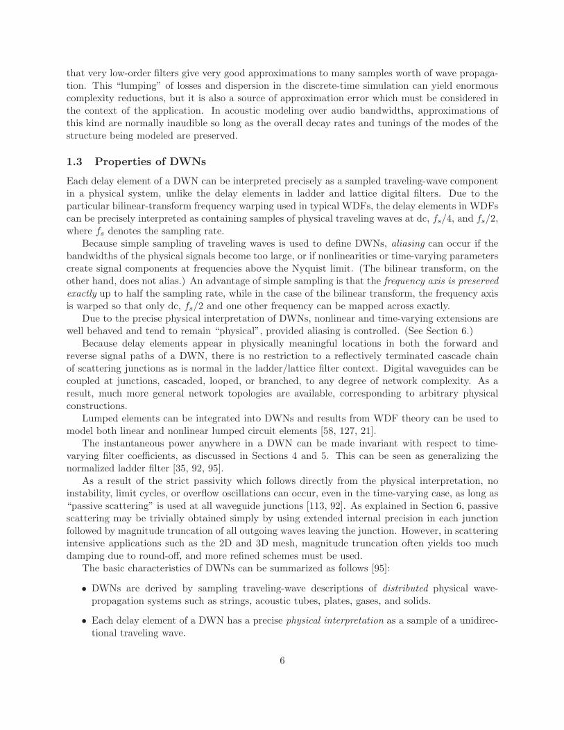
1.3 Properties of DWNs

Each delay element of a DWN can be interpreted precisely as a sampled traveling-wave componentin a physical system, unlike the delay elements in ladder and lattice digital filters. Due to theparticular bilinear-transform frequency warping used in typical WDFs, the delay elements in WDFscan be precisely interpreted as containing samples of physical traveling waves at dc, fs/4, and fs/2,where fs denotes the sampling rate.

Because simple sampling of traveling waves is used to define DWNs, aliasing can occur if thebandwidths of the physical signals become too large, or if nonlinearities or time-varying parameterscreate signal components at frequencies above the Nyquist limit. (The bilinear transform, on theother hand, does not alias.) An advantage of simple sampling is that the frequency axis is preservedexactly up to half the sampling rate, while in the case of the bilinear transform, the frequency axisis warped so that only dc, fs/2 and one other frequency can be mapped across exactly.

Due to the precise physical interpretation of DWNs, nonlinear and time-varying extensions arewell behaved and tend to remain “physical”, provided aliasing is controlled. (See Section 6.)

Because delay elements appear in physically meaningful locations in both the forward andreverse signal paths of a DWN, there is no restriction to a reflectively terminated cascade chainof scattering junctions as is normal in the ladder/lattice filter context. Digital waveguides can becoupled at junctions, cascaded, looped, or branched, to any degree of network complexity. As aresult, much more general network topologies are available, corresponding to arbitrary physicalconstructions.

Lumped elements can be integrated into DWNs and results from WDF theory can be used tomodel both linear and nonlinear lumped circuit elements [58, 127, 21].

The instantaneous power anywhere in a DWN can be made invariant with respect to time-varying filter coefficients, as discussed in Sections 4 and 5. This can be seen as generalizing thenormalized ladder filter [35, 92, 95].

As a result of the strict passivity which follows directly from the physical interpretation, noinstability, limit cycles, or overflow oscillations can occur, even in the time-varying case, as long as“passive scattering” is used at all waveguide junctions [113, 92]. As explained in Section 6, passivescattering may be trivially obtained simply by using extended internal precision in each junctionfollowed by magnitude truncation of all outgoing waves leaving the junction. However, in scatteringintensive applications such as the 2D and 3D mesh, magnitude truncation often yields too muchdamping due to round-off, and more refined schemes must be used.

The basic characteristics of DWNs can be summarized as follows [95]:

• DWNs are derived by sampling traveling-wave descriptions of distributed physical wave-propagation systems such as strings, acoustic tubes, plates, gases, and solids.

• Each delay element of a DWN has a precise physical interpretation as a sample of a unidirec-tional traveling wave.

6

• The frequency axis is preserved up to half the sampling rate (i.e., it is not warped accordingto the bilinear transform).

• Physically meaningful nonlinear, time-varying extensions are straightforward.

• Aliasing can occur due to nonlinearities, time variation, or inadequate bandlimiting of initialconditions and/or input signals.

• Fully general modeling geometries are available (e.g., in contrast to ladder/lattice filters).

• Lumped models can be simply interfaced to DWNs.

• Overall signal energy can be simply controlled.

• Instability, limit cycles, can overflow oscillations can be suppressed by using “passive scatter-ing.”

• Sensitivity to coefficient quantization can be minimized.

• A synthesis procedure exists for constructing any single-input, single-output (SISO) transferfunction by means of a DWN [111], and any m-input, k-output transfer function by meansof a multivariable DWN [112].

1.4 Paper Outline

Section 2 gives a generalized formulation of waveguide models: After a short introduction in classicalterms, we consider the m-component dual variables p and u, which can be associated with anyphysical wave quantities such as acoustic pressure and volume velocity, or voltage and current.This discrete-time multivariable formulation, while leading to results similar to those in classicalelectrical network theory [4], provides a general framework giving a unified treatment of variousmodeling problems.

In Section 3, we define the lossless junction of waveguide sections in terms of energy conservation.Such a formulation yields a class of lossless scattering junctions larger than that arising from theset of all physically meaningful scattering junctions.

Section 4 discusses power normalization of waveguide variables, and the results are applicableto both physical and non-physical scattering junctions.

In Section 5, we summarize formulas for physical, normalized, and unnormalized scatteringjunctions of m-variable waveguide branches. We show how these junctions can be loaded with alumped network and present an example in acoustic modeling.

In Section 6, using the physical interpretation of the computations, we give conditions forensuring passivity of nonlinear and time-varying DWNs.

In Section 7, we present an algebraic analysis of the lossless junction, and the fundamental con-dition of losslessness is translated into the domain of eigenvalues and eigenvectors of the scatteringmatrix.

Section 8 shows how physical junctions can be implemented efficiently, both in the normalizedand unnormalized cases. As a byproduct, two new three-multiply, three-add normalized latticesections are derived. It is shown that the proposed implementations are robust with respect tocoefficient quantization, and dynamic range requirements are addressed.

7

Section 9 considers an abstract geometric (as opposed to physically geometric) interpretationof physical scattering computations. The normalized scattering matrix is shown to be equivalentto a Householder reflection, while the unnormalized case can be seen as an oblique Householderreflection. Householder matrices are highly valued in numerical analysis because they conserve nu-merical dynamic range and thereby yield robust algorithms [34]. As a byproduct of this viewpoint,another new three-multiply, three-add normalized lattice section is derived which is especially wellsuited for implementation on general-purpose digital signal processing chips.

For completeness, Section 10 briefly covers the extension of lossless scattering and junction nor-malization to the case in which scattering matrices may contain complex rational transfer functionelements. Such cases arise in the computational modeling of acoustic systems such as intersectingconical tubes and woodwind fingerholes. Junctions loaded by an arbitrary lumped impedance (e.g.,a Helmholtz resonator mouthpiece model or complex violin bridge impedance), can also be handledthis way.

2 Basic DWN Formulation

This section reviews the DWN paradigm and briefly outlines considerations arising in acousticsimulation applications.

The formulation is based on dual m-dimensional vectors of “pressure” and “velocity” p andu, respectively. These variables can be associated with acoustic pressure and particle- or volume-velocity, or they can be anything analogous such as electrical voltage and current, mechanical forceand velocity, etc. We call these dual variables Kirchhoff variables to distinguish them from wavevariables which are their traveling-wave components. For concreteness, we will focus on pressureand velocity waves in a lossless, linear, acoustic tube. In acoustic tubes, velocity waves are in unitsof volume velocity (particle velocity times the tube cross-sectional area) [60].

2.1 The Ideal Acoustic Tube

First we address the scalar case. For an ideal acoustic tube, we have the following wave equation [60]:

∂2p(x, t)

∂t2= c2 ∂2p(x, t)

∂x2(1)

where p(x, t) denotes (scalar) pressure in the tube at the point x along the tube at time t in seconds.If the length of the tube is LR, then x is taken to lie between 0 and LR. We adopt the conventionthat x increases “to the right” so that waves traveling in the direction of increasing x are referred toas “right-going.” The constant c is the speed of sound propagation in the tube, given by c =

√

K/µ,where K is the “spring constant” or “stiffness” of the air in the tube,2 and µ is the mass per unitvolume of the tube. The dual variable, volume velocity u, also obeys (1) with p replaced by u. Thewave equation (1) also holds for an ideal string, if p represents the transverse displacement, K isthe tension of the string, and µ is its linear mass density.

The wave equation (1) follows from the more physically meaningful telegrapher’s equations [24]:

− ∂p(x, t)

∂x= µ

∂u(x, t)

∂t(2)

2“Stiffness” is defined here for air as the reciprocal of the adiabatic compressibility of the gas [61, p. 230]. Thisdefinition helps to unify the scattering formalism for acoustic tubes with that of mechanical systems such as vibratingstrings.

8

−∂u(x, t)

∂x= K−1 ∂p(x, t)

∂t(3)

Equation (2) follows immediately from Newton’s second law of motion, while (3) follows fromconservation of mass and properties of an ideal gas [61].

The general traveling-wave solution to (1), (2), and (3) was given by D’Alembert [60] as

p(x, t) = p+(x− ct) + p−(x + ct)u(x, t) = u+(x− ct) + u−(x + ct)

(4)

where p+, p−, u+, u− are the right- and left-going wave components of pressure and velocity, re-spectively, and are referred to as wave variables. This solution form is interpreted as the sum oftwo fixed wave-shapes traveling in opposite directions along the uniform tube. The specific wave-shapes are determined by the initial pressure p(x, 0) and velocity u(x, 0) throughout the tube forx ∈ [0, LR].

2.2 Multivariable Formulation of the Acoustic Tube

A straightforward multivariable generalization of the telegrapher’s equations (2) and (3) gives thefollowing m-variable generalization of the wave equation (5):

∂2p(x, t)

∂t2= KM−1 ∂2p(x, t)

∂x2(5)

in the spatial coordinates xT △=[

x1 . . . xm

]

at time t, where M and K are m×m non-singular,

non-negative matrices which play the respective roles of multidimensional mass and stiffness. Thesecond spatial derivative is defined here as

[

∂2p(x, t)

∂x2

]T△=

[

∂2p1(x, t)

∂x21

. . .∂2pm(x, t)

∂x2m

]

(6)

For digital waveguide modeling, we desire solutions of the multivariable wave equation whichinvolve only sums of traveling waves, because traveling wave propagation can be efficiently simulateddigitally using only delay lines, digital filters, and scattering junctions. Consider the eigenfunction

p(x, t) =

est+v1x1

. . .est+vmxm

△= estI+V X · 1 (7)

where s is interpreted as a Laplace-transform variable s = σ + jω, I is the m×m identity matrix,

X△=diag(x), V

△=diag([v1, . . . , vm]) is a diagonal matrix of spatial Laplace-transform variables (the

imaginary part of vi being spatial frequency along the ith spatial coordinate), and 1T △=[1, . . . , 1].

Substituting the eigenfunction (7) into (5) gives the algebraic equation

s2I = KM−1V 2 △= C2V 2 (8)

where C is the diagonal matrix of sound-speeds along the m coordinate axes. Since C2V 2 = s2I,we have

V = ±sC−1. (9)

9

Substituting (9) into (7), the eigensolutions of (5) are found to be of the form

p(x, t) = es

(

tI±C−1X)

· 1 (10)

Having established that (10) is a solution of (5) when condition (8) holds for the matrices M

and K, we can express the general traveling-wave solution to (5) in both pressure and velocity as

p(x, t) = p+ + p−

u(x, t) = u+ + u− (11)

where p+△=f(tI−C−1X), with f being an arbitrary superposition of right-going components of the

form (10) (i.e., taking the minus sign), and p−△=g(tI + C−1X) is similarly any linear combination

of left-going eigensolutions from (10) (all having the plus sign). Similar definitions apply for u+

and u−. When the time and space arguments are dropped as in the right-hand side of (11), it isunderstood that all the quantities are written for time t and position x.

When the mass and stiffness matrices M and K are diagonal, our analysis corresponds toconsidering m separate waveguides as a whole. For example, the three directions of vibration (onelongitudinal and two transverse) in a single terminated string can be described by (5) with m = 3.The coupling among the strings occurs primarily at the bridge in a piano [132]. As we will seelater, the bridge acts like a junction of several multivariable waveguides.

When the matrices M and K are non-diagonal, the physical interpretation can be of the form

C2 △= KM−1 (12)

where K is the stiffness matrix, M is the mass density matrix. C is diagonal if (8) holds, and inthis case, the wave equation (5) is decoupled in the spatial dimensions. There are physical examples

where the matrices M and K are not diagonal, even though C2 △= KM−1 is. One such example,

in the domain of electrical variables, is given by m conductors in a sheath or above a ground plane,where the sheath or the ground plane acts as a coupling element [63, pp. 67–68].

Note that the multivariable wave equation (5) considered here does not include wave equationsgoverning propagation in multidimensional media (such as membranes, spaces, and solids). Inhigher dimensions, the solution in the ideal linear lossless case is a superposition of waves travelingin all directions in the m-dimensional space [60]. However, it turns out [122] that a good simulationof wave propagation in a multidimensional medium may be in fact be obtained by forming a mesh ofunidirectional waveguides as considered here, each described by (5). Such a mesh of 1D waveguidescan be shown to solve numerically a discretized wave equation for multidimensional media [125].

2.3 Generalized Wave Impedance

From the multivariable generalization of (2), we have, using (10), ∂p(x, t)/∂x = −M∂u(x, t)/∂t⇒±sC−1p = −sMu⇒ p = ±CMu = ±K1/2M1/2u

△= ±Ru, where ‘+’ is for right-going and ‘−’

is for left-going. Thus, following the classical definition for the scalar case, the wave impedance isdefined by

R△= K1/2M1/2 = CM

10

and we havep+ = Ru+

p− = −Ru− (13)

Thus, the wave impedance R is the factor of proportionality between pressure and velocity in atraveling wave. It is diagonal if and only if the mass matrix M is diagonal (since C is assumeddiagonal). The minus sign for the left-going wave p− accounts for the fact that velocities mustmove to the left to generate pressure to the left. The wave admittance is defined as Γ = R−1.

More generally, when there is a loss represented by a diagonal matrix G, we have, in thecontinuous-time case,

p = eGXes

(

tI−C−1X)

· 1 (14)

where X△= diag(x) as before, leading to the admittance matrix

Γ = M−1C−1 − 1

sM−1G (15)

For the discrete-time case, we may map Γ(s,x) from the s plane to the z plane via the bilineartransform [65], or we may sample the inverse Laplace transform of Γ(s,x) and take its z transformto obtain Γ(z, x).

A linear propagation medium in the discrete-time case is completely determined by its waveimpedance R(z, x) (generalized here to permit frequency-dependent and spatially varying waveimpedances). A waveguide is defined for purposes of this paper as a length of medium in whichthe wave impedance is either constant with respect to spatial position x, or else it varies smoothlywith x in such a way that there is no scattering (as in the conical acoustic tube). For simplicity,we will suppress the possible spatial dependence and write only R(z).3

2.4 Generalized Complex Signal Power

The net complex power involved in the propagation can be defined as [4]

P = u∗p = (u+ + u−)∗(p+ + p−)

= u+∗Ru+ − u−∗

R∗u− +

u−∗Ru+ − u+∗

R∗u−

△= (P+ − P−) + (P× − P×∗) (16)

where all quantities above may be functions of z, and “∗” denotes paraconjugation (transpositionand complex conjugation on the unit circle in the z plane). The quantity P+ = u+∗

Ru+ iscalled right-going active power (or right-going average dissipated power4), while P− = u−∗

R∗u−

3There are no tube shapes supporting exact traveling waves other than cylindrical and conical (or conical wedge,which is a hybrid) [69]. However, the “Salmon horn family” (see, e.g., [60, 96]) characterizes a larger class ofapproximate “one-parameter traveling waves.” In the cone, the wave equation is solved for pressure p(x, t) using achange of variables p′ = px, where x is the distance from the apex of the cone, causing the wave equation for thecone to reduce to that of the cylindrical case [2].

4Note that |z| = 1 corresponds to the average physical power at frequency ω, where z = exp(jωT ), and the wavevariable magnitudes on the unit circle may be interpreted as RMS levels [4, p. 48]. For |z| > 1, we may interpretthe power P(z) = u∗(1/z∗)p(z) as the steady state power obtained when exponential damping is introduced into thewaveguide giving decay time-constant τ , where z = exp(−T/τ) exp(jωT ) [4, p. 48].

11

is called the left-going active power. The term P+−P−, the right-going minus the left-going powercomponents, we call the net active power, while the term P× − P×∗ is net reactive power. Thesenames all stem from the case in which the matrix R(z) is positive definite for |z| ≥ 1. In this case,both traveling components of the active power are real and positive, the active power itself is real,and the reactive power is purely imaginary.

2.5 Medium Passivity

Following the classical definition of passivity [4, 133], a medium is said to be passive if

P+ + P− ≥ 0 (17)

for |z| ≥ 1. Thus, a sufficient condition for ensuring passivity in a medium is that each travelingactive-power component be real and non-negative.

To derive a definition of passivity in terms of the wave impedance, consider a perfectly reflectinginterruption in the transmission line, such that u− = u+. For a passive medium, using (16), (17)becomes

R(z) + R∗(1/z∗) ≥ 0 (18)

for |z| ≥ 1. The wave impedance R(z) is an m-by-m function of the complex variable z. Condition(18) is essentially the same thing as saying R(z) is positive real [128], except that it is allowed tobe complex (but Hermitian), even for real z.5 The matrix R∗(1/z∗) is the paraconjugate of R,i.e., the unique analytic continuation (when it exists) of the Hermitian transpose of R from theunit circle to the complex z plane [110]. Since the inverse of a positive-real function is positivereal, the corresponding generalized wave admittance Γ(z) = R−1(z) is positive real (and henceanalytic) in |z| ≥ 1. In other terms, the sum of the wave impedance and its paraconjugate ispositive semidefinite.

We say that wave propagation in the medium is lossless if the wave impedance matrix satisfies

R(z) = R∗(1/z∗) (19)

i.e., if R(z) is para-Hermitian (which implies its inverse Γ(z) is also).Most applications in waveguide modeling are concerned with nearly lossless propagation in

passive media. In this paper, we will state results for R(z) in the more general case when applicable,while considering applications only for constant and diagonal impedance matrices R. As shown inSection 2.3, coupling in the wave equation (5) implies a non-diagonal impedance matrix, since thereis usually a proportionality between the speed of propagation C and the impedance R through thenon-diagonal matrix M .

The wave components of equations (11) travel undisturbed along each axis. This propagationis implemented digitally using m bidirectional delay lines, as depicted in Fig. 1. We call such acollection of delay lines an m-variable waveguide section. Waveguide sections are then joined attheir endpoints via scattering junctions (discussed further in following sections) to form a DWN.

5A complex-valued function of a complex variable f(z) is said to be positive real if

1) z real ⇒ f(z) real

2) |z| ≥ 1 ⇒ Re{f(z)} ≥ 0

Positive real functions characterize passive impedances in classical network theory [129].

12

p (t)+

z-mL

z-m

L

p (t + m T)-

+p (t - m T)

L

L

p (t)-

p (t)+

z-mL

z-m

L

p (t + m T)-

+p (t - m T)

L

L

p (t)-

1 1

11

m

m

m

m

Figure 1: An m-variable waveguide section.

2.6 Impulsive Signals Interpretation

Let c denote the speed of propagation in one branch of an m-variable waveguide section having real,positive wave impedance R. Let L be the linear length of this branch in samples. The propagationtime from one end to the other is Tp = L/c. If Tp = nT , where T is the sampling interval of thedigital network, the (frequency-independent) propagation in the branch can be precisely simulated(ignoring any roundoff errors due to scattering at the endpoints). Extending this restriction to everybranch in the network, we can state that a DWN is equivalent to a physical waveguide networkin which the input pressure signals are streams of weighted impulses at intervals of T seconds.This equivalence is also true in the case of time-varying wave impedances. The impulsive nature ofthe propagating signals serves to sample the junction scattering coefficients at the digital samplinginstants.

2.7 Bandlimited Signals Interpretation

A more practically useful correspondence between physical and digital waveguide networks is ob-tained by assuming the inputs to the physical networks are bandlimited continuous-time Kirchoffvariables. The signals propagating throughout the physical network are assumed to consist of fre-quencies less than fs/2 Hz, where fs = 1/T denotes the sampling rate. Therefore, by the Shannonsampling theorem, if we record a sample of the pressure wave, say, at each unit-delay element everyT seconds, the bandlimited continuous pressure fluctuation can be uniquely reconstructed through-out the waveguide network. Saying the pressure variation is frequency bandlimited to less thanfs/2 is equivalent to saying the pressure distribution is spatially bandlimited to less than fs/2c, or,a one-sample section of waveguide is less than half a cycle of the shortest wavelength contained ina traveling wave. In summary, a DWN is equivalent to a physical waveguide network in which theinput signals are bandlimited to fs/2 Hz. This equivalence does not remain true for time-varyingor non-linear DWNs.

13

In the case of time-varying wave impedances, the time-variation of the resultant scattering coef-ficients applies a continuous amplitude modulation to the continuous propagating signals, therebygenerating sidebands. If the signals incident on a junction are bandlimited to f1 Hz and the scat-tering coefficients are bandlimited to f2 Hz, then the signals emerging from an interconnectionof waveguides are bandlimited only to f1 + f2 Hz. If the network is nontrivial, a portion of theamplitude-modulated signals may return to the same time-varying junction, and the signal band-width expands to f1 + 2f2, and so on. A time-varying junction eventually expands the bandwidthof the signals contained in the network to infinity. With a fixed sampling rate fs in the DWN,we obtain aliased versions of the physical signals. The general result is that time-varying physicalwaveguide networks cannot be simulated by DWNs at a fixed sampling rate. In practice, however,we obtain good approximate digital simulations by working with wave variables and junction pa-rameters bandlimited to much less than fs/2, and by using sufficient damping (implemented usinglow-pass filtering) in the network so that the aliased signal energy is attenuated below significance.

Particular care must be used also when inserting nonlinear elements into waveguide networks,since they also extend the bandwidth, and frequency foldover will result. Nonlinear elements arealmost always present in the excitation blocks of musical instruments (e.g., reeds, bows, and felt-covered hammers), sometimes also in the resonators (e.g., brasses, sitar strings and cymbals), andsometimes also in the output amplification/diffusion stage (e.g., a saturating amplifier or speakersimulation). Nonlinearities in the resonators (such as a sitar string) may be sufficiently weak so thatinherent low-pass filtering can attenuate nonlinearly generated high frequencies to insignificancebefore they alias. Also, nonlinear excitations can be bandlimited using a lowpass filter if they arenot strongly coupled to the resonator they excite (the “source-filter” decomposition). Similarly,nonlinearities in the output path can be implemented without aliasing in the absence of feedbackto the resonator or excitation. In some practical cases, conditions for the passivity of nonlinearitiescan be determined [127, 62, 81]. However, preventing aliasing is much more difficult. One strategyis to use low-order polynomials to implement nonlinearities. A polynomial of order n expands thebandwidth by only a factor of n. Therefore, bandlimiting the nonlinearity input to fs/(2n) andoversampling by a factor of n will avoid aliasing.

A third reason (beyond time-variation and nonlinearity support) for adopting a sampling ratesignificantly higher than the audio frequency bandwidth is the necessity of using fractional delays.These are needed whenever a high spatial resolution is needed, or when the waveguide length mustbe “continuously” variable. In all these cases digital interpolators must be used, in the form ofFIR or IIR filters, ideally allpass (see next subsection). To some extent, both FIR and IIR filtertypes introduce amplitude and/or phase distortion at high frequencies, so it is typically beneficialto increase the sampling rate and provide a “guard band” between 20 kHz (for high fidelity audio)and fs/2.

2.8 Interpolated Digital Waveguides

Integer delay lengths are not sufficient for musical tuning of digital waveguide models at commonlyused sampling rates [40]. The simplest scheme which is typically tried first is linear interpolation.However, poor results are obtained in some cases (such electric guitar models) due to the pitch-dependent damping caused by delay-line interpolation. As is well known [88], linear interpolationis equivalent to a time-varying FIR filter of the form y(n) = α(n)x(n) + [1 − α(n)]x(n − 1), andfor α(n) = 0.5 (for interpolation half way between available samples), the gain of the interpolationfilter at fs/2 drops to zero. In some cases, such as for steel string simulation, the interpolation filter

14

becomes the dominant source of damping, so that when the pitch happens to fall on an integerdelay-line length (α = 0), the damping suddenly decreases, making the note stand out as “buzzy.”In such cases, something better than linear interpolation is required.

Allpass interpolation is a nice choice for the nearly lossless feedback loops commonly used indigital waveguide models [40, 104], because it does not suffer any frequency-dependent damping.Its phase distortion normally manifests as a slight mistuning of high-frequency resonances, which isusually inaudible and arguably even desirable in most cases. However, allpass interpolation insteadhas the problem that instantly switching from one delay to another (as in a “hammer-on” or “pull-off” simulation in a string model) gives rise to a transient artifact due to the recursive nature of theallpass filter. Transient artifacts can be reduced or eliminated by “warming up” a second instanceof the filter using the new coefficients in advance of the transition (ideally several time-constantsin advance) and, at the desired transition time, switching out the old filter and switching in thenew [120]. In this way, the new filter is switched in with state consistent with the new coefficients.Another approach is to cross-fade from the old filter to the new filter, allowing consistent state todevelop in the new filter before its output fades in.

Another popular choice is Lagrange interpolation [46, 115, 1, 88] which is a special case ofFIR filter interpolation; while the transient artifact problem is minimal since the interpolatingfilter is nonrecursive, there is still a time-varying amplitude distortion at high frequencies. In fact,first-order Lagrange interpolation is just linear interpolation, and higher orders can be shown togive a maximally smooth frequency response at dc (zero frequency), while the gain generally rollsoff at high frequencies. Allpass interpolation can be seen as trading off this frequency-dependentamplitude distortion for additional frequency-dependent delay distortion [13]. A comprehensivereview of Lagrange interpolation appears in [115].

Both allpass and FIR interpolation suffer from some delay distortion at high frequencies due tohaving a nonlinear phase response at non-integer desired delays. As mentioned above for the allpasscase alone, this distortion is normally inaudible, even in the first-order case, causing mistuning orphase modulation only in the highest partial overtones of a resonating string or tube.

Optimal interpolation can be approached via general-purpose bandlimited interpolation tech-niques [105, 70]. However, the expense is generally considered too high for widespread usage atpresent. Both amplitude and delay distortions can be eliminated over the entire band of humanhearing using higher order IIR (e.g., allpass) or FIR interpolation filters in conjunction with someamount of oversampling. A comprehensive review of delay-line interpolation techniques is given in[53].

2.9 Lossy, Dispersive Waveguides

In reality, distributed linear propagation is never lossless. There is always some attenuation anddispersion per unit distance traveled by a wave in the medium. In principle, implementing loss anddispersion calls for a digital filter to be inserted at the output of every delay element to preciselysimulate one sample of wave propagation. In practice this is generally unnecessary. Instead, wemay normally implement digital filters sparsely along each digital waveguide [97, 99]. Each filterprovides the attenuation and dispersion corresponding to the propagation distance over the sectionit covers. In other words, lossy, dispersive media are approximated by piecewise lossless mediahaving the same average attenuation and dispersion over long distances. Loss and dispersion arethus lumped at sparse points along the waveguide model rather than being lumped at each spatialsampling point.

15

In the 1D case, it is possible to obtain exact results using sparsely lumped losses and dispersion,thanks to the commutativity of linear, time-invariant elements [99]. For example, consider anacoustic cylinder which is L samples long. If the per-sample traveling-wave filter is given by Hs(z),and if we only care what happens at the endpoints of the tube, then we need only implement thefilter HL

s (z) at each end of the L-sample tube, prior to any junctions. Since the per-sample filteringHs(z) is typically very weak, the stronger filter HL

s (z) is normally also quite weak and readilyapproximated to within audio specifications by a low-order digital filter.

It is easy to show that the per-sample traveling-wave filter Hs(z) for any passive propagationmedium such as a string or acoustic cylinder must satisfy

∣∣Hs(e

jω)∣∣ ≤ 1 for all ω ∈ [−π, π]. That

is, wave propagation in a fixed wave impedance cannot increase traveling-wave amplitude at anyfrequency. This is a convenient stability criterion which is straightforward to ensure in practice.

In summary, wave propagation in a general linear time-invariant medium is thus simulated usinga (possibly interpolated) delay line to handle the time-delay associated with the propagation, andone or more digital filters to sparsely implement losses and dispersion where needed, such as priorto a bow-string contact model [90].

2.10 The General Linear Time-Invariant Case

Let y(t, x) denote the transverse displacement, in one plane, of a vibrating string [60]. The completelinear time-invariant generalization of the lossy, stiff string is described by the differential equation

∞∑

k=0

αk∂ky(t, x)

∂tk=

∞∑

l=0

βl∂ly(t, x)

∂xl. (20)

which, on setting y(t, x) = est+vx, (or taking the 2D Laplace transform with zero initial conditions),yields the algebraic equation,

∞∑

k=0

αksk =

∞∑

l=0

βlvl. (21)

Solving for v in terms of s is, of course, nontrivial in general. However, in specific cases, wecan determine the appropriate attenuation per sample G(ω) and wave propagation speed c(ω) bynumerical means. For example, starting at s = 0, we normally also have v = 0 (corresponding to theabsence of static deformation in the medium). Stepping s forward by a small differential j∆ω, theleft-hand side can be approximated by α0 +α1j∆ω. Requiring the generalized wave velocity s/v(s)to be continuous, a physically reasonable assumption, the right-hand side can be approximated byβ0 + β1∆v, and the solution is easy. As s steps forward, higher order terms become important oneby one on both sides of the equation. Each new term in v spawns a new solution for v in terms ofs, since the order of the polynomial in v is incremented. For each solution v(s), let vr(ω) denotethe real part of v(jω) and let vi(ω) denote the imaginary part. Then the eigensolution familycan be seen in the form exp {jωt± v(jω)x} = exp {±vr(ω)x} · exp {jω (t± vi(ω)x/ω)}. Defining

c(ω)△=ω/vi(ω), and sampling according to x → xm

△=mX and t → tn

△=nT (ω), with X

△=c(ω)T (ω),

(the spatial sampling period is taken to be frequency invariant, while the temporal sampling intervalis modulated versus frequency using allpass filters), the left- and right-going sampled eigensolutionsbecome

ejωtn±v(jω)xm = e±vr(ω)xm · ejω[tn±xm/c(ω)]

= Gm(ω) · ejω(n±m)T (ω) (22)

16

where G(ω)△=e±vr(ω)X . Thus, a general map of v versus s, corresponding to a partial differential

equation of any order in the form (20), can be translated, in principle, into an accurate, local, linear,time-invariant, discrete-time simulation. The boundary conditions and initial state determine theinitial mixture of the various solution branches as is typical in, say, the stiff string [19].

In summary, a large class of wave equations with constant coefficients, of any order, admits a de-caying, dispersive, traveling-wave type solution. Even-order time derivatives give rise to frequency-dependent dispersion and odd-order time derivatives correspond to frequency-dependent losses.Higher order spatial derivatives can be approximated by higher order time derivatives and treatedsimilarly [10]. The corresponding digital simulation of an arbitrarily long (undriven and unobserved)section of 1D medium (such as a string or acoustic tube) can be simplified via commutativity to atmost two pure delays and at most two linear, time-invariant filters. In higher dimensions, such asfor the 2D mesh, the per-sample filtering cannot in general be exactly commuted to the boundariesof the mesh. However, an approximation problem can be solved which matches the observed modalfrequencies and decay rates using sparsely distributed low-order filters in an otherwise lossless mesh(e.g., around the rim).

In practical physical simulation scenarios, such as for real-world strings or acoustic tubes, it isgenerally most effective to identify experimentally the attenuation and dispersion associated withwave propagation at each frequency over the band of interest [108, 49]. These data can be used todesign a digital filter which gives an optimal approximation over the propagation distance desired.If needed, the per-sample filter identified in this way can be translated into higher-order termsin the wave equation for the medium. Thus, the wave equation itself can be “identified” frommeasured input-output behavior of the medium (assuming it is linear and uniform) rather thanbeing derived from physical principles and physical constants of the medium as is classically done[61, 11].

3 The Lossless Junction

A scattering junction of waveguide sections is characterized by its scattering matrix A. The rela-tionship between the N incoming and outgoing traveling waves is given by:

p− = Ap+ (23)

where p+ is the vector of incoming waves (assumed scalar here) and p− is the vector of outgoingwaves relative to the junction (see Fig. 2). We say that the junction is N -way (or it has N branches)if N is the dimension of the incoming and outgoing wave vectors.

We now consider the case of a constant scattering matrix A. The more general case of scatteringmatrices as functions of z will be considered in Section 10.

The net complex power entering the junctions is

P = u∗p = p+∗Γ∗(1/z∗)p+ − p−∗Γp− +

p+∗Γ∗(1/z∗)p− − p−∗Γp+

= (P+ − P−) + (P× − P×∗) (24)

where Γ is the diagonal matrix containing the N wave admittances of all the branches meeting atthe junction. Assuming the branch admittances are Hermitian and nonzero, we have that Γ haspositive real elements along its diagonal and zeros elsewhere. The quantity P+ = p+∗Γp+ ≥ 0 is

17

p1+p1

-

p2+

p2- p3

+

p3-

A

Figure 2: A schematic depiction of the 3-way waveguide junction.

incoming active power, and P− = p−∗Γp− ≥ 0 is then the outgoing active power relative to thejunction. The term P+ − P− is the absorbed active power, while the term P× − P×∗, containingthe mixed incoming and outgoing waves, is called the reactive power.

A scattering junction is said to be passive when the absorbed active power is nonnegative, i.e.,when

P+ ≥ P− (25)

for |z| ≥ 1. In other terms, the outgoing active power does not exceed the incoming active power.

3.1 Generalized Lossless Scattering

A scattering junction is said to be lossless if P+ = P−, i.e., the active power absorbed at thejunction is zero. In the case of lossless propagation in a passive medium, it is easy to verifyfrom (19), (23) and (24) that this is ensured if and only if

Γ(z) = A∗Γ(z)A (26)

where Γ(z) is a generalized wave admittance which is para-Hermitian and analytic for |z| > 16. Inthis case the matrix A is said to be a lossless scattering matrix. We refer to (26) as the conditionof losslessness.

When wave propagation occurs in a medium which is passive but not necessarily lossless, thecondition for lossless scattering becomes

Γ∗(1/z∗) = A∗Γ(z)A (27)

Notice that (26) is closely related to the well-known

6Note that by the maximum modulus theorem, if a matrix of meromorphic functions is positive definite on theunit circle and analytic outside the unit circle, it is necessarily positive definite everywhere outside the unit circle.

18

Lyapunov equation [43] for testing the asymptotic stability of discrete-time linear systems.The definition of lossless junctions employed here includes junctions arising from the connection

of physical waveguides, and extends the formal treatment to non-physical junctions as well. Incertain applications, it can be useful to use non-physical scattering matrices having a particularstructure which increases the computational efficiency, or which gives the desired behavior of thesystem [78, 79].

In DWNs, waveguide sections separating scattering junctions are normally implemented usingdelay lines. Since in any physical simulation there will be delay in both directions, the delay linesisolate the scattering junctions, allowing parallel computation of the junctions. This is an advantageover traditional ladder/lattice filters in which delay elements are present in only one flow direction[57, 92], thus preventing both a direct pipelined computation and a physical interpretation. On theother hand, having the delays along only one direction is easier to work with when the problem isto realize a ladder/lattice filter having a prescribed transfer function [57, 112].

4 The Normalized Lossless Junction

In some applications it is worthwhile to normalize the traveling waves so that all waveguideseffectively have unit impedance, R(z) = I. To normalize, pressure waves are multiplied by a(matrix) square root of the wave admittance, and velocity waves are multiplied by a (matrix)square root of the wave impedance. Conservation of power at a lossless junction implies that thesignal dynamic range is conserved in a mean square sense for normalized waves. This can be veryuseful in fixed-point implementations of large networks, especially in the time-varying case, sincesignal scaling problems are avoided and the full dynamic range can be achieved at every point ofthe network. Normalized waveguide networks can be seen as a generalization of the normalizedladder filter [35].

4.1 Time-Varying Normalized Waveguide Networks

A time-varying waveguide network can be created by changing one or more impedances over time.This induces changes in the scattering junctions connecting the various impedances. Defining timevariation this way also preserves the physical interpretation of the time-varying network which iscritical for keeping a handle on passivity and hence on stability and numerical robustness.

Since the signal power associated with, say, a single traveling pressure sample p(n) storedwithin a delay element in a scalar digital waveguide is Pp(n) = p2(n)Γ, where Γ is the (scalar)wave admittance of the associated waveguide, modulating a waveguide impedance also modulatesthe stored signal power in that waveguide. That is, the stored power associated with the samplep(n) varies proportional to Γ(n). This is not the case with normalized waves. The normalizedcounterpart of pressure sample p(n) is p(n) = p(n)

√

Γ(n), and the associated power is always justthe square of the sample value: Pp(n) = p2(n) = p2(n)Γ(n) = Pp(n). The scattering junctionsconnecting normalized waveguides are modulated by the time-varying impedances, but the storedsignal power in the normalized waveguides is not. For the case of lossless scattering junctions,signal energy is constant throughout the time-varying network. This gives a general class of energyconserving time-varying digital filters which, along with passive rounding rules, are also free of limitcycles and overflow oscillations [92]. Thus, normalized waveguide networks decouple signal powerin the network from time variations in the scattering coefficients: A change in the wave impedance

19

changes the scattering properties of the junctions but does not alter the instantaneous signal powerin the network.

4.2 Isolating Time-Varying Junctions

Since waveguide sections are typically terminated on both ends by scattering junctions, a changein one waveguide impedance modulates both scattering junctions rather than only one as maybe desired. It is possible to vary the coefficients of only a single junction when the network isan acyclic graph (which can be thought of as a generalization of the cascade chain as used inladder/lattice filters). Consider the simple case of the cascade chain: Suppose there are N wave-guides abutted end to end and numbered 1 through N from left to right. Suppose further that wewant to modulate only the scattering junction between sections m and m + 1. We can accomplishthis by modulating the impedance Rm+1 of section m+1. Let the modulation signal be denoted byg(n) = Rm+1(n)/Rm+1(0), assuming the modulation begins after time 0. Then we can cancel themodulation at the right endpoint of section m + 1 by modulating the impedance of section m + 2by g(n) (since the scattering coefficients at the junction of two waveguides depends only on theimpedance ratio). However, now we have to also modulate the impedance of section m + 3 by g(n)in order to prevent modulation at the junction of sections m + 2 and m + 3. Continuing in thisway, we must modulate the impedances of all waveguides to the right of section m by g(n) in orderto obtain an isolated modulated junction between sections m and m + 1. This argument extendsreadily to an acyclic graph, and breaks down whenever a “downstream” branch is connected to an“upstream” branch, i.e., whenever there is a cycle in the waveguide network graph.

The simultaneous variation of many wave impedances determines an instantaneous variationof the stored signal power. When the waveguides are normalized, the signal power remains fixed.As a result, it is possible to vary isolated junctions in the normalized case without worrying aboutenergy modulation consequences in other parts of the network.

Another way to isolate impedance variations in a time-varying network is by means of idealtransformers which can step the wave impedance up or down by an arbitrary factor without inducingreflections. The basic theory of the digital waveguide transformer is discussed in Appendix A, andSection 9 discusses further applications.

4.3 Scattering of Normalized Waves

We consider first diagonal impedance matrices, since they have an intuitive physical counterpart inlossless acoustic tubes. Under this assumption, we have the impedance matrix

R = diag[R1, . . . , Rn] (28)

and the admittance matrixΓ = diag[Γ1, . . . ,Γn] = R−1. (29)

By (19) and the assumption of a passive medium, the normalized pressure waves are uniquelydefined as

p±i =p±i√Ri

= p±i√

Γi (30)

where the three signs above are all taken as “+” or all as “−”. (Square roots in this paper arealways taken as positive.) We can write also

p± = Γ1

2 p± (31)

20

where Γ1

2 is the diagonal square root of Γ. The junction of normalized waveguides is in this caserepresented by the scattering matrix

A = Γ1

2 AΓ− 1

2 (32)

As a side note, this equation is analogous to the relation between power-wave scattering matri-ces and voltage-wave scattering matrices as found in the WDF literature [27] for lumped circuitelements.

In the more general case, when the (complex) admittance matrix Γ is not necessarily diagonal,but remains positive semidefinite as required for lossless propagation, we have that Γ admits aCholesky factorization

Γ = U∗U (33)

where U is upper triangular. We can define the normalized pressure waves as

p± = Up± (34)

The normalized scattering junction is obtained via the following similarity transformation on theunnormalized scattering matrix:

A = UAU−1 (35)

Theorem 1 The scattering matrix of a normalized junction is unitary, i.e.,

A∗A = I (36)

Proof: From the condition of losslessness (26), we have A∗A = U−∗A∗U∗UAU−1 = U−∗A∗ΓAU−1 =

U−∗ΓU−1 = U−∗U∗UU−1 = I

By an explicit computation of the matrix product in (36) we can show that the terms of anycolumn of A are power complementary, i.e.,

N∑

i=1

| ai,k |2 = 1 (37)

for all k.

5 Physical Scattering Junctions

All scattering matrices arising from the connection of N scalar physical waveguides have the samebasic structure which is an efficient subset of the set of all lossless scattering matrices in the senseof (26). To fix the setting, consider the parallel junction of N lossless acoustic tubes, each with real,positive, scalar wave admittance Γi. The pressure at the junction is the same for all N waveguidesat the junction point, and the velocities from each branch sum to zero. These physical constraintsyield scattering matrices of the form

A =

2Γ1

ΓJ− 1 2Γ2

ΓJ. . . 2ΓN

ΓJ

2Γ1

ΓJ

2Γ2

ΓJ− 1 . . . 2ΓN

ΓJ

. . .2Γ1

ΓJ

2Γ2

ΓJ. . . 2ΓN

ΓJ− 1

△= 1αT − I (38)

21

where ΓJ and α are defined as follows:

ΓJ =N∑

i=1

Γi (39)

α△=

2

ΓJ[Γ1, . . . ,ΓN ]T (40)

It is easy to verify that the matrix A satisfies the condition of losslessness (26). In the particularcase of equal-impedance waveguides, we have

Ae =

2N − 1 2

N . . . 2N

2N

2N − 1 . . . 2

N. . .2N

2N . . . 2

N − 1

△=

2

N11T − I (41)

We notice that the elements of each row of matrix A in (38) and (41) are allpass complementary,i.e., |∑N

k=1 ai,k | = 1, for all k. Since the scattering matrix Ae for equal-impedance waveguides issymmetric, the elements of any row or column of matrix Ae are allpass complementary. Since Ae

remains unchanged in the normalized case, the elements of each row and column are also powercomplementary.

The equal-impedance case is particularly important when N is a power of two. In this case,all the multiplications can be replaced by right-shifts in fixed-point arithmetic, and considerablesavings in circuit area can be achieved in a VLSI implementation. This case has been explored inthe design of efficient digital waveguide meshes [91, 122, 125].

The scattering matrix for a connection of N normalized physical waveguides is given by (32).It can be more explicitly written as

A =

2Γ1

ΓJ− 1 2

√Γ1Γ2

ΓJ. . . 2

√Γ1ΓN

ΓJ

2√

Γ2Γ1

ΓJ

2Γ2

ΓJ− 1 . . . 2

√Γ2ΓN

ΓJ

. . . . . .

. . . . . .2√

ΓNΓ1

ΓJ

2√

ΓNΓ2

ΓJ. . . 2ΓN

ΓJ− 1

△= 2γγT − I (42)

where γ△= 2√

ΓJ[√

Γ1, . . . ,√

ΓN ]T , and the power-complementary property (37) can be verified for

both rows and columns.In the expressions (38)–(42), the elements of the matrices are real, since the one-variable wave-

guides intersecting at the junction have real, positive impedances.Normalized N -way scattering junctions represented by real matrices can be implemented by

N(N −1)/2 CORDIC processors [38]. Since the scattering matrix is orthogonal (real and unitary),it corresponds to a rotation in N dimensions. Any such rotation can be obtained by N(N − 1)/2

22

planar rotations [34], with each planar rotation being realizable using a CORDIC processor. Thisformulation can be useful for VLSI implementations.

The junction represented by the expressions (38) to (42) is formally a parallel junction. Thecorresponding series junction can be obtained by taking the dual of the parallel junction, i.e.,by replacing admittance with impedance and interchanging pressure and velocity. In the seriesjunction, the velocity is the same in all waveguides at the junction, and the pressures (or forces)sum to zero.

Parallel junctions occur naturally in the case of intersecting acoustic tubes, while series junctionsarise at the intersection of N transversely vibrating strings, where the transverse velocity must bethe same for all N strings. For waves in strings, force waves play the role of pressure waves inacoustic tubes. Note that the wave equation (1) for strings is usually written in terms of transversedisplacement. However, choosing velocity and force as Kirchhoff variables unifies the treatment ofvibrating strings with that of acoustic tubes.

5.1 Parallel Junction of Multivariable Complex Waveguides

We now consider the scattering matrix for the parallel junction of N m-variable physical waveguides,and at the same time, we treat the generalized case of matrix transfer-function wave impedances.Equations (13) and (11) can be rewritten for each m-variable branch as

u+i = Γi(z) p+

i

u−i = − Γ∗

i (1/z∗) p−i

(43)

andui = u+

i + u−i

pi = p+i + p−

i = pJ1(44)

where Γi(z) = R−1i (z), pJ is the pressure at the junction, and we have used pressure continuity to

equate pi to pJ for any i.Using conservation of velocity we obtain

0 = 1TN∑

i=1

ui

= 1TN∑

i=1

{

[Γi(z) + Γ∗i (1/z∗)] p+

i

−Γ∗i (1/z∗)pJ1}

(45)

and

pJ = S1TN∑

i=1

[Γi(z) + Γ∗i (1/z∗)] p+

i (46)

where

S =

{

1T

[N∑

i=1

Γ∗i (1/z∗)

]

1

}−1

. (47)

23

Hence, the scattering matrix is given by

A = S

1T[

Γ1 + Γ∗1 . . . ΓN + Γ∗

N

]

. . .

1T[

Γ1 + Γ∗1 . . . ΓN + Γ∗

N

]

− I (48)

It is clear that (38) is a special case of (48) when m = 1. If the branches do not all have the samedimensionality m, we may still use the expression (48) by letting m be the largest dimensionalityand embedding each branch in an m-variable propagation space.

5.2 Loaded Junctions

In discrete-time modeling of acoustic systems, it is often useful to attach waveguide junctions toexternal dynamic systems which act as a load. We speak in this case of a loaded junction. The loadis expressed in general by its complex admittance and can be considered a lumped circuit attachedto the distributed waveguide network.

Examples of loaded junctions can be found in certain representations of finger holes in wind-instrument modeling [93, 80], or in bridge terminations in stringed-instrument modeling [98] (see theexample in the next section). They are also a natural way to load a waveguide mesh to simulate airabove a membrane [31]. Sometimes the load can be time-varying and even nonlinear, as in the caseof a piano hammer hitting a string [127, 7]; in this case, the hammer is modeled as a mass-springsystem in which the spring stiffness nonlinearly depends on its compression, and the impedance“seen” by the string changes continuously during contact. Finally, the loaded junction equationscan be used to interface a DWN with other types of physical modeling simulations (e.g., a WDF):In such a case, the attached load is simply the driving-point impedance of the external simulation.

To derive the scattering matrix for the loaded parallel junction of N lossless acoustic tubes,the Kirchhoff’s node equation is reformulated so that the sum of velocities meeting at the junctionequals the exit velocity (instead of zero). For the series junction of transversely vibrating strings,the sum of forces exerted by the strings on the junction is set equal to the force acting on the load(instead of zero).

The load admittance ΓL is regarded as a lumped driving-point admittance [128], and the equation

UL(z) = ΓL(z)pJ(z) (49)

expresses the relation at the load. In acoustic modeling applications, ΓL is normally first obtained inthe continuous-time case as a function of the Laplace transform variable s. Denote the continuous-time Laplace transform by Γc

L(s), and the inverse Laplace transform by γcL(t). To preserve the

tuning of audio resonances of acoustic systems, the load admittance is usually converted to discretetime by the impulse-invariant method, i.e., simple sampling of γc

L(t) in the time domain. In simplercases in which there is only one resonance to be transformed from the s plane to the z plane,such as a piano-hammer model (a mass-spring system) or the individual terms of a partial fractionexpansion, the bilinear transform s = α(z − 1)/(z + 1) may be used [65].

In the impulse-invariant case, to avoid aliasing, we require ΓcL ≃ 0 for frequencies near and

above half the sampling rate. Since the driving-point admittances of acoustic systems are notgenerally bandlimited (consider the driving-point impedance of an elementary mass Γc

L(s) = 1/msor spring Γc

L(s) = Ks), anti-aliasing filtering should be applied to γcL(t). The bilinear transform is

24

inherently free of aliasing since the entire jω axis in the s plane is mapped only once to the unitcircle in the z plane, but as a result of this mapping, the frequency axis is warped, and the behaviorat continuous-time frequencies can be mapped to the same discrete-time frequencies at only threepoints (dc, half the sampling rate, and one more frequency which is arbitrary). For this reason, theimpulse-invariant method is normally preferred when the precise tuning of more than one spectralfeature is important.

In case of a time-varying or nonlinear load, as in the piano-hammer model, to avoid aliasing, theload impedance should vary sufficiently slowly and/or be sufficiently weakly nonlinear so that thelow-pass filtering in the DWN will attenuate modulation and/or distortion products to insignificancebefore aliasing occurs in the recursive network.

The scattering matrix for a loaded parallel junction of N lossless, scalar waveguides with realwave impedances can be rewritten as [93]

AL =

2Γ1

ΓJ− 1 2Γ2

ΓJ. . . 2ΓN

ΓJ

2Γ1

ΓJ

2Γ2

ΓJ− 1 . . . 2ΓN

ΓJ

. . . . . .

. . . . . .2Γ1

ΓJ

2Γ2

ΓJ. . . 2ΓN

ΓJ− 1

where

ΓJ = ΓL +N∑

i=1

Γi (50)

For the more general case of N m-variable physical waveguides, the expression of the scatteringmatrix is that of (48), with

S =

[

1T

(N∑

i=1

Γi

)

1 + ΓL

]−1

(51)

5.3 Example: Bridge Coupling of Piano Strings

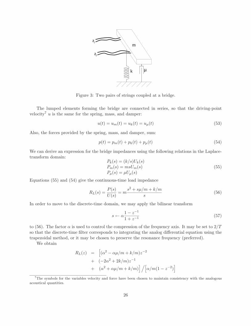
As an application of the theory, we outline the digital simulation of two pairs of piano strings. Thestrings are attached to a common bridge which acts as a coupling element between the strings (seeFig. 3). An in-depth treatment of coupled strings can be found in [132].

To a first approximation, the bridge can be modeled as a lumped mass-spring-damper system,while for the strings, a distributed waveguide representation is more appropriate. For the purposeof illustrating the theory in its general form, we represent each pair of strings as a single 2-variablewaveguide. This approach is justified if we associate the pair with the same key in such a way thatboth the strings are subject to the same excitation. Since the 2×2 matrices M and T of (5) can beconsidered to be diagonal in this case, we could alternatively describe the system as four separatescalar waveguides.

The ith pair of strings is described by the 2-variable impedance matrix

Ri =

[

Ri,1 00 Ri,2

]

(52)

25

mz

z

µk

1

2

Figure 3: Two pairs of strings coupled at a bridge.

The lumped elements forming the bridge are connected in series, so that the driving-pointvelocity7 u is the same for the spring, mass, and damper:

u(t) = um(t) = uk(t) = uµ(t) (53)

Also, the forces provided by the spring, mass, and damper, sum:

p(t) = pm(t) + pk(t) + pµ(t) (54)

We can derive an expression for the bridge impedances using the following relations in the Laplace-transform domain:

Pk(s) = (k/s)Uk(s)Pm(s) = msUm(s)Pµ(s) = µUµ(s)

(55)

Equations (55) and (54) give the continuous-time load impedance

RL(s) =P (s)

U(s)= m

s2 + sµ/m + k/m

s(56)

In order to move to the discrete-time domain, we may apply the bilinear transform

s← α1− z−1

1 + z−1(57)

to (56). The factor α is used to control the compression of the frequency axis. It may be set to 2/Tso that the discrete-time filter corresponds to integrating the analog differential equation using thetrapezoidal method, or it may be chosen to preserve the resonance frequency (preferred).

We obtain

RL(z) =[

(α2 − αµ/m + k/m)z−2

+ (−2α2 + 2k/m)z−1

+ (α2 + αµ/m + k/m)]/[

α/m(1− z−2)]

7The symbols for the variables velocity and force have been chosen to maintain consistency with the analogousacoustical quantities.

26

The factor S in the impedance formulation of the scattering matrix (48) is given by

S(z) =

2∑

i,j=1

Ri,j + RL(z)

−1

(58)

which is a rational function of the complex variable z. The scattering matrix is given by

A = 2S

R1,1 R1,2 R2,1 R2,2

R1,1 R1,2 R2,1 R2,2

R1,1 R1,2 R2,1 R2,2

R1,1 R1,2 R2,1 R2,2

− I (59)

which can be implemented using a single second-order filter having transfer function (58).

6 Nonlinear, Time-Varying DWNs

The DWN paradigm is highly useful for constructing time-varying nonlinear digital filters whichare guaranteed stable in the Lyapunov sense [59, 25]. Lyapunov stability analysis involves findinga positive-definite “Lyapunov function” (which is like a norm defined on the filter state), whichdecreases each time step (given zero inputs) in the presence of linear or nonlinear computations(such as numerical round-off). Whenever each state variable (delay element) in a filter computationhas a physical interpretation as an independent wave variable, a Lyapunov function can be definedsimply as the sum of wave energies associated with the state variables. By choosing the scattering-junction round-off rules to be passive (e.g., by using magnitude truncation), the total stored energyin the filter decreases or remains the same relative to an infinite-precision implementation. Aslong as the infinite-precision filter is asymptotically stable, the quantized filter must be also. Thus,the total stored energy in any “physical” digital filter is precisely what is needed for a Lyapunovfunction.

Since many ladder, lattice, and wave digital filters are equivalent to DWNs, possibly after somedelay manipulations [51, 92, 93, 75], it is clear that DWNs can be used to realize a wide class oftransfer functions. In particular, every filter transfer function can be realized as a linear combinationof DWNs (in a manner analogous to using “tap parameters” on a ladder or lattice filter [57, 12]), andlinear combinations are well behaved in the presence of nonlinearities and time-varying parameters.

In practice, Lyapunov stability in a DWN is normally guaranteed by ensuring that wave-variables are never amplified by nonlinear operations or time-varying gains. For example, magnitudetruncation on each output of an extended-precision scattering junction suffices to ensure passivity.Non-amplifying nonlinearities and varying gains are sufficient for passivity but sometimes too dissi-pative, especially in waveguide mesh applications [122]. A more refined rule is obtained by summingrounded-off energy (or an approximation to it) in an accumulator and changing the direction ofrounding so as to servo the cumulative energy error to zero [93].

In the normalized case, the energy associated with each signal sample in a DWN is given bythe square of that sample,8 so the total energy stored in a DWN is given simply as the sum of

8Strictly speaking, a squared wave variable in a normalized waveguide is proportional to signal power [97], andwe should multiply by the sampling interval T to obtain units of energy. However, such a constant scale factor isinconsequential.

27

squares of all the samples contained in all the delay elements. In the unnormalized case, the energyof the jth sample xi,j(n) in waveguide i, at time n, is given by x2

i,j(n)/Ri, where Ri is the waveimpedance of the ith waveguide, and the total energy at time n in the DWN can be written as

E(n) =N∑

i=1

Mi∑

j=1

x2i,j(n)

Ri.

where Mi is the length of waveguide i in samples. The DWN is stable in the presence of time-varying nonlinearities so long as E(n) (the Lyapunov functional for the DWN) is not increasedwhen all inputs are zero, i.e.,

E(n + 1) ≤ E(n).

Thus, magnitude truncation (rounding toward zero) at the output of all scattering junctions (withextended precision internal to each junction) preserves network stability, as does multiplication ofany wave variable by a nonlinear or time-varying gain gi,j(n) not exceeding 1 in magnitude, i.e.,we only require |gi,j(n)| ≤ 1, for all n.

The above general result is applied in the following specific example (which is related to awaveguide sitar model):

( )ny( )[ ]nyng ,

z−N

Allpass ( )zA

Figure 4: A feedback loop containing a delay line, an allpass filter, and a time-varying nonlinearity.

Theorem 2 A feedback loop containing an allpass filter A(z) (assumed here to be exactly imple-mented), a delay line of any length N > 0, and a time-varying nonlinearity g[n, y(n)], as shown inFig. 4, is stable in the Lyapunov sense if |g[n, y(n)]| ≤ 1 for all n. If the initial stored energy isE(0), then the total energy remaining at time n is given by

E(n) = E(0)−n∑

i=1

{1− g2[i, y(i)]}y2(i)

Proof: It suffices to show that (a) the arrangement of Fig. 4 is numerically equivalent to aDWN, and (b) y(n) is a wave variable of the DWN corresponding to a unit impedance. Considerthe redrawing of Fig. 4 as in Fig. 5. The delay line is broken into two halves to form a digitalwaveguide. (If the delay line length is odd, a sample of delay can be moved in cascade with theallpass filter.) It is well known that an arbitrary order M allpass filter can be realized in the form ofa digital ladder filter [57] with no “taps,” and it is straightforward to show that such a ladder filtercan be manipulated into a digital waveguide filter by splitting each unit delay into two half-delaysand commuting half of the half-delays around the ladder so that there is a half-delay between each

28

scattering junction on both the upper and lower rails of the lattice [92].9 In this configuration,also shown in Fig. 5, the ladder filter is a DWN consisting of a cascade of digital waveguides,where the input and output of the allpass are the incoming and outgoing wave variables at the leftof the leftmost waveguide of the allpass, and the rightmost waveguide is terminated on the rightby a perfect reflection (infinite wave impedance, given pressure or force waves). Without loss ofgenerality, we may choose the wave impedance of the bidirectional delay line to be 1. The returnsignal y(n) from the allpass is a wave variable at wave impedance 1, and its energy at time n isy2(n). After scaling by the nonlinearity, its energy becomes |g[n, y(n)]|2y2(n), and the energy losteach sample interval is therefore {1− g2[n, y(n)]}y2(n), which is nonnegative, and the total energylost is simply the sum over time of these per-sample losses.

k1 − k1

1 − k1

1 + k1

R1R0 = 1

z−N 2

z−N 2 ( )[ ]nyng ,

z− 21

z− 21( )ny

{ {

DigitalWaveguide

NonlinearityAllpass filter in Kelly-Lochbaum DWN form

z− 21

z− 21

…

…kM − kM

1 − kM

1 + kM

RM ∞

Figure 5: A system equivalent to Fig. 4 containing a bidirectional delay line (digital waveguide)terminated reflectively on the left, terminated on the right by an allpass reflectance, and containinga time-varying nonlinearity on the return wave from the allpass.

Corollary 1 All lossless nonlinearities or time-varying gains in the system of Fig. 4 can only selectbetween the values +1 and −1.

Corollary 2 The amplitude of y(n) is bounded by y(n) ≤√

E(n).

Corollary 3 The signal y(n) will approach zero asymptotically so long as |g[n, y(n)]| ≤ 1 − ǫ forsome fixed ǫ > 0, irrespective of how g may vary with time or as a function of y.

Of course, by keeping track of the energy gained or lost, as illustrated in the above theorem,and by controlling the gain/nonlinearity so that energy gained or lost is compensated at a latertime, a wider class of nonlinear and/or time-varying systems may be defined which are lossless onaverage. An example is the exactly lossless (on average) DWN which servos round-off error energyto zero mentioned above. It is also possible to approximate lossless nonlinear behavior within theallpass filter [67, 127].

9Altering a ladder filter to convert it to a DWN can also be accomplished using the cut-set method of Kung[51, 12].

29

7 Algebraic Properties of Lossless Junctions

Comparing (38) and (42) shows that the elements of the normalized scattering matrix A in (42)are

ai,j = ai,j

√Γi√Γj

= 2√

ΓiΓj

/N∑

k=1

Γk − δ(i− j) = aj,i (60)

where δ(n)△=1 for n = 0 and 0 for n 6= 0. Hence, the normalized scattering matrix A is symmetric.

As was shown in Theorem 1, it is easy to verify by direct computation that A is also unitary (i.e.,AA

∗= A

∗A = I), so that all its eigenvalues are on the unit circle. Since all eigenvalues of a real,

symmetric matrix are real [66], A has eigenvalues only at ±1. Moreover, since by (32) A and A

are related by a similarity transformation, A also must have all eigenvalues at +1 or −1.An elementary eigenvector analysis can be conducted using physical analogies. It is well known

that a symmetric matrix has orthogonal eigenvectors. For the equal-impedance case, one eigenvector

is always e0 =[

1 1 . . . 1]T

by symmetry: this corresponds to a collision of equal pressure

waves at the junction, so the return scatter must be identical. This corresponds to the eigenvalue 1.For the -1 eigenvalues, a similar interpretation can be found: inject a unit pressure wave at all thebranches but one, and “pull out” a pressure wave having magnitude N−1 at the remaining branch.In this case, the return scatter is inverted, since we have arranged that the pressure be zero at thejunction and hence at each branch termination. In this way we can find N eigenvectors analogous

with e1 =[

−(N − 1) 1 . . . 1]T

which span the (N −1)-dimensional subspace associated with

the eigenvalue -1. Note that e0 is orthogonal to this subspace, while the ei are not mutuallyorthogonal for i > 0.

For unequal impedances, a similar physical interpretation can be found for the eigenvectors.If we supply equal pressure waves to all branches at the junction, the reflected waves must beequal by symmetry, since p−i = pJ − p+

i , where pJ is the junction pressure and all the p+i are

equal. Hence, e0 =[

1 1 . . . 1]T

remains an eigenvector corresponding to the eigenvalue

1. On the other hand, if we inject a unit pressure wave into all the branches but the jth and“pull out” a pressure wave having magnitude

∑

i6=j Γi/Γj at the jth branch, then the junctionpressure pJ is again forced to zero by construction and the return scatter at any branch is thenegative of the incoming wave on that branch. In this way we can find N eigenvectors analogous

with ej =[

1 . . . 1 −∑i6=j Γi/Γj 1 . . . 1]T

spanning the (N − 1)-dimensional subspace

associated with the eigenvalue -1. In this case, none of the eigenvectors is necessarily orthogonalto the others.

The foregoing is an example of how physical intuition can help in finding algebraic propertiesof a given matrix in physical applications.

Another property of the scattering matrix A is that it is its own inverse: A2 = I. Thiscorresponds physically to the fact that if the results of a scattering operation are fed back to thesame junction as incoming waves, the result must be the inverse of the original scattering. Animplication of this is that lossless scattering networks can be run in reverse, i.e., by changing thedirections of all the delay lines and computing the junctions as dictated by the wave impedances, thenetwork will compute its own inverse. If there are inputs and outputs, they must be interchanged.

30

7.1 Conditions for Lossless Scattering

We now present a theorem characterizing the condition of losslessness in terms of the eigenvaluesand eigenvectors of the scattering matrix.

Theorem 3 A scattering matrix A ∈ CN×N is lossless if and only if its eigenvalues lie on the unitcircle and it admits a basis of N linearly independent eigenvectors.

Proof: By definition (26), A is lossless if A∗ΓA = Γ, where Γ is a positive definite matrix.Therefore, Γ admits a Cholesky factorization Γ = U∗U where U is an upper triangular matrixwhich converts A to a unitary matrix via similarity transformation: A∗ΓA = Γ ⇒ A∗U∗UA =U∗U ⇒ A

∗A = I, where

A = UAU−1 (61)

This shows the eigenvalues of every lossless scattering matrix lie on the unit circle. It readily followsfrom similarity to A that A admits N linearly independent eigenvectors.

Conversely, assume |λi| = 1 for each eigenvalue λi of A, and that there exists a matrix T oflinearly independent eigenvectors of A. Then the matrix T diagonalizes A to give T−1AT = D ⇒T ∗A∗T−1∗ = D∗, where D = diag(λ1, . . . , λN ). Multiplying, we obtain T ∗A∗T−1∗T−1AT =D∗D = I ⇒ A∗T−1∗T−1A = T−1∗T−1. Thus, the condition of lossless scattering (26) is satisfiedfor Γ = T−1∗T−1 which is Hermitian and positive definite.

Theorem 3 can be extended to lossless junctions of lossy waveguides, as the reader can easilyverify by applying the above proof to (27).

It is worth noting that most research in feedback delay networks for artificial reverberation hasbeen concerned only with orthogonal feedback matrices [42, 33] rather than on the more general classof matrices satisfying the losslessness condition (26) [78, 106, 79]. This is an excessive restrictionsince many of the matrices naturally arising from models of lossless physical junctions are notorthogonal. As can be seen above, physical scattering matrices are orthogonal only if we restrictattention to propagation in equal-admittance media [Γ(z) = I], or to propagation of normalizedwaves.

8 Complexity Reduction: A Physical Approach

The scattering matrix of a physical junction of N waveguides (38) can be expressed in terms of thealpha parameters as

A = 1αT − I (62)

where αT =[

α1 α2 . . . αN

]

, and in the lossless case,

αi△=2Γi

/N∑

j=1

Γj . (63)

The vector of outgoing pressure waves can be expressed as

p− = Ap+ △= 1pJ − p+ (64)

where pJ = αT p+ can be interpreted as the “junction pressure.” Thus, the matrix-vector multipli-cation can be seen to require only N multiplications and 2N − 1 additions.

31

Equation (64) can be rewritten as

pJ =N∑

i=1

αip+i , αi

△=

2Γi

Γ1 + · · ·+ ΓN

p−j = pJ − p+j (65)

This is the canonical form of the scattering relations for a physical N -way scattering junctionparametrized in terms of the alpha parameters.

Whenever possible, it is advisable to set the branch impedances so that αi = 1 for some i,and therefore only N − 1 multiplications are needed. This is achieved when the ith waveguideadmittance equals the sum of all the other admittances. According to Fettweis’ terminology forwave digital filters, the ith junction port is called a reflection-free port, and the ith branch is saidto be adapted to the other N − 1 branches. Physically, a wave traveling into the junction on areflection-free port will be fully scattered into the other branches meeting at the junction, with noreflection back along branch i.

In time-varying applications, it is also convenient to maintain scaling such that∑N

j=1 Γj = 1so that no divisions or renormalizations are necessary in the alpha parameters. This is easilyaccomplished by setting the admittance of branch 1, say, to

Γ1(n) = 1−N∑

i=2

Γi(n) (66)

provided this remains nonnegative.Since the alpha parameters sum to 2 in the lossless case, the first element, say, of the vector α

can be expressed as

α1 = 2−N∑

i=2

αi (67)

Thus, the vector of outgoing pressure waves can be computed as

p− = 1αT p+ − p+

= 1

(

2p+1 −

N∑

i=2

αip+1 +

N∑

i=2

αip+i

)

− p+

= 1

[

2p+1 +

N∑

i=2

αi(p+i − p+

1 )

]

− p+ (68)

which implies

p−j = 2p+1 +

N∑

i=2

αi(p+i − p+

1 )− p+j

= p−1 − (p+j − p+

1 )︸ ︷︷ ︸

available

(69)

In Fettweis’ terminology, the port corresponding to the first waveguide is called the dependentport. Organizing the computations as in (68), a scattering junction can be performed with N − 1

32

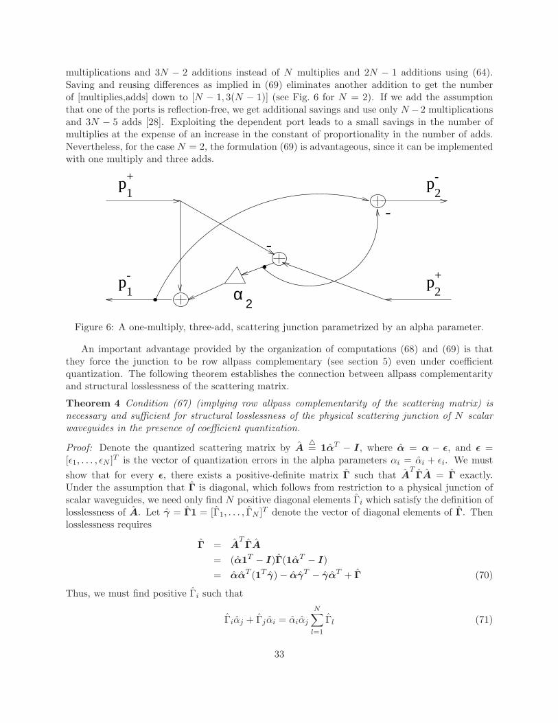
multiplications and 3N − 2 additions instead of N multiplies and 2N − 1 additions using (64).Saving and reusing differences as implied in (69) eliminates another addition to get the numberof [multiplies,adds] down to [N − 1, 3(N − 1)] (see Fig. 6 for N = 2). If we add the assumptionthat one of the ports is reflection-free, we get additional savings and use only N −2 multiplicationsand 3N − 5 adds [28]. Exploiting the dependent port leads to a small savings in the number ofmultiplies at the expense of an increase in the constant of proportionality in the number of adds.Nevertheless, for the case N = 2, the formulation (69) is advantageous, since it can be implementedwith one multiply and three adds.

-

-

p

pp

+

+

p-

-

1

1

2

2α2

Figure 6: A one-multiply, three-add, scattering junction parametrized by an alpha parameter.

An important advantage provided by the organization of computations (68) and (69) is thatthey force the junction to be row allpass complementary (see section 5) even under coefficientquantization. The following theorem establishes the connection between allpass complementarityand structural losslessness of the scattering matrix.

Theorem 4 Condition (67) (implying row allpass complementarity of the scattering matrix) isnecessary and sufficient for structural losslessness of the physical scattering junction of N scalarwaveguides in the presence of coefficient quantization.

Proof: Denote the quantized scattering matrix by A△= 1αT − I, where α = α − ǫ, and ǫ =

[ǫ1, . . . , ǫN ]T is the vector of quantization errors in the alpha parameters αi = αi + ǫi. We must

show that for every ǫ, there exists a positive-definite matrix Γ such that ATΓA = Γ exactly.

Under the assumption that Γ is diagonal, which follows from restriction to a physical junction ofscalar waveguides, we need only find N positive diagonal elements Γi which satisfy the definition oflosslessness of A. Let γ = Γ1 = [Γ1, . . . , ΓN ]T denote the vector of diagonal elements of Γ. Thenlosslessness requires

Γ = ATΓA

= (α1T − I)Γ(1αT − I)

= ααT (1T γ)− αγT − γαT + Γ (70)

Thus, we must find positive Γi such that

Γiαj + Γjαi = αiαj

N∑

l=1

Γl (71)

33

Let Γi = cαi/2 where c is any positive constant. Since αi is positive, so is Γi. (While αi is restrictedto certain values, Γi may be any positive real value). The condition (71) becomes

αiαjc = αiαjcN∑

l=1

αl/2 (72)

which holds if and only ifN∑

l=1

αl = 2 (73)

and this identity is provided by condition (67).We see that exact losslessness of a physical waveguide junction is assured provided only that

the actual alpha parameters are positive and sum precisely to 2 after quantization. The proofextends readily to nonnegative αi by assigning Γi = 0 to any waveguide branch corresponding to aport for which αi = 0. (Note that αi = 0 corresponds to a branch which contributes no signal tothe junction, and a branch with zero admittance can convey no signal power. Such a situation isphysically degenerate so that if quantization forces αi to zero for some i, the corresponding branchmay be removed from the junction.)

The above theorem is quite simple from a physical point of view: All we require for exactlosslessness is that the quantized scattering matrix correspond to some valid lossless scatteringmatrix. From the physical correspondence (63) between the alpha parameters and the branch waveadmittances it is clear that losslessness holds when α1 + · · ·+ αN = 2. For more general passivity,we can add a positive real “load” admittance ΓL to the sum over Γj above to obtain that scatteringpassivity holds if and only if the alpha parameters are positive and sum to a value not exceeding 2.

The above discussion is only concerned with passivity of the scattering matrix itself. Theapplication of the matrix is assumed to be exact. Since rounding of the final outgoing waves isnecessary in practice, we add

Corollary 4 Sufficient conditions for the passivity of a DWN are (1) all scattering matrices arepassive, (2) intermediate outgoing waves are computed exactly at each junction in extended precisionbefore rounding, and (3) the final outgoing waves from each junction are rounded passively.

Since extended intermediate precision is required to ensure passivity, it is of interest to examinethe additional bits required.

Theorem 5 For an order N junction with m-bit alpha parameters (m > 1) and n-bit scalar wavevariables (n > 2) computed in fixed point, the extended precision needed to implement the canonicalscattering formula (64) is (a) one additional bit for the computation of junction pressure pJ , and(b) two additional bits for the computation of each outgoing wave p−j .

Proof: From (64), assuming 0 < αi ≤ 2 and −1 ≤ p+i < 1, we have

|pJ | =∣∣∣∣∣

N∑

i=1

αip+i

∣∣∣∣∣≤

N∑

i=1

αi

∣∣∣p+

i

∣∣∣ <

N∑

i=1

αi ≤ 2

Hence (a) one additional bit is sufficient for the inner-product accumulator for pJ . That the extrabit is necessary is shown by taking p+

i = −1 for all i in which case pJ = −2 for any set of losslessalpha parameters.

34

The outgoing wave variables are computed as p−i = pJ − p+i , and a single bit is clearly sufficient

to provide the needed headroom for a single subtraction in general. That the second headroom bit isnecessary is shown by considering the example N = 2, α1 = 0, α2 = 2, p+

1 = 1/2, p+2 = −1, in which

case p−1 = −2 − 1/2 = −2.5. If α1 = 0 is not allowed, then an example is obtained with α1 = ǫ1,α2 = 2−ǫ1, p+

1 = −1, p+2 = 1−ǫ2, for which p−1 = (ǫ1−1)(−1)+(2−ǫ1)(1−ǫ2) = 3−2ǫ1−2ǫ2+ǫ1ǫ2.

For this to exceed 2, we must have 2ǫ1 + 2ǫ2 − ǫ1ǫ2 < 1. With m = 3 or more, we can chooseǫ1 = 1/4, and with n = 3 or more, we can take ǫ2 = 1/4, and the inequality is satisfied. Thus, (b)two extra bits are necessary and sufficient for the computation of each outgoing wave variable p−j .

It is perhaps surprising at first that only one extra bit suffices for the junction pressure compu-tation, no matter how many branches are impinging on the junction. Ordinarily, an inner productof length N requires log2(N) headroom bits. The single headroom bit requirement is a direct resultof the alpha parameters being restricted to positive partitions of 2 in the lossless case, or a positivepartitioning of a positive number less than 2 in the lossy, passive case.

Since an out-of-range outgoing traveling wave typically must be “clipped” in practice (i.e.,replaced by −1 if negative and 1 − ǫ2 if positive), the two extra carry bits are normally fed alongwith the next lower bit (the in-range sign bit) to saturation logic which implements clipping asneeded.

The computations (68) or (69) can also be used to implement precisely lossless or passive time-varying junctions. In this case, the passivity constraints become

N∑

i=2

αi(n) ≤ 2

αi(n) ≥ 0 (74)

where n is time in samples, since α1 implicitly obeys (67) in formulas (68) and (69). (Here weallow αi(n) = 0 which may be a convenient way to eliminate waveguide branches momentarily inthe time-varying case.)

A junction of normalized waveguides can be obtained from (68) or (69) by transformer-couplingeach branch other than the first with a waveguide having wave admittance Γ1. The ideal transformerintroduces two additional multiplications for each branch except one. Therefore, the normalizedjunction for arbitrary impedances can be implemented using 3(N −1) multiplications and 3(N −1)additions.

8.1 The Three-Multiply Normalized Lattice Section.

A well known two-port unnormalized scattering junction [57], implemented using one multiply andthree adds, can be derived by organizing (64) as

p−1 = p+2 + p∆

p−2 = p+1 + p∆

(75)

wherep∆

△= ρ(p+

1 − p+2 ), (76)

and

ρ△= α1 − 1 = 1− α2 =

Γ1 − Γ2

Γ1 + Γ2=

R2 −R1

R2 + R1(77)

35

is the reflection coefficient seen at an impedance step from R1 to R2, i.e., at port 1. In theladder/lattice filter literature, only a 4-multiply, 2-add normalized junction appears to be known.A normalized, three-multiply junction can be obtained simply by coupling any one-multiply junctionsuch as (75) with an ideal transformer [92] (see Appendix A), as illustrated in Fig. 7, where

g△=√

Γ2/Γ1 (78)

However, any lossless two-port junction which preserves a physical interpretation will do. Forexample, a transformer can also be attached to the alpha-parametrized one-multiply junction ofFig. 6 to obtain the three-multiply normalized junction of Fig. 8, having essentially the sameproperties as that of Fig. 7.

p2-

p2+

p

p

+

-

1

1ρ

-

g

1/g

Figure 7: A three-multiply, three-add, normalized scattering junction parametrized in terms of areflection coefficient.

p2-

p2+

-

-

p

p

+

-

1

1 α2

g

1/g

Figure 8: A three-multiply, three-add, normalized junction parametrized in terms of an alphaparameter.

Note that a high quality sinusoidal oscillator requiring only one multiply can be formed by

36

adding a unit delay on either side of a three-multiply junction and reflectively terminating (inwhich case the transformer multiplies cancel) [103].

One-multiply two-port scattering junctions enforce structural losslessness in finite precisionarithmetic since the allpass complementarity condition (67) is always true. A normalized junctionobtained by transformer-normalizing a one-multiply junction is also structurally lossless, providedthe transformer multipliers are implemented in extended precision. In practice, normalized junc-tions of this type are made passive by using any non-amplifying rounding rule at the output.

Denoting the ideal transformer coefficients by g−△=√

Γ2/Γ1 and g+ = 1/g−, the passivity conditionon the transformer with quantized coefficients g− = g− − ǫ− and g+ = g+ − ǫ+ is g+g− ≤ 1, evenin the time-varying case.

Since one of the transformer coefficients is always greater than 1, fixed-point implementationsrequire support for an integer part, unlike the fractional fixed-point format used in most DSP chips.Since the transformer commutes with the junction in the two-port case, the larger coefficient can,without loss of generality, be chosen to apply to the signal entering the junction. As an example ofthe increased internal dynamic range required, if ρ ∈ [−1+ǫ, 1−ǫ], the transformer coefficients maybecome as large as

√

2/ǫ− 1. If ǫ is the “machine epsilon,” i.e., ǫ = 2−(n−1) for typical n-bit two’scomplement arithmetic normalized to lie in [−1, 1), then the dynamic range of the transformercoefficients is bounded by

√2n − 1 ≈ 2n/2. In summary, while transformer-normalized junctions

trade a multiply for an add in the two-port case, they require up to 50% more bits of dynamicrange within the junction adders.

9 Complexity Reduction: A Geometric Approach

A convenient expression for the scattering matrix of a junction of N normalized waveguides isobtained in terms of

uTn

△=[ √

Γ1

√Γ2 . . .

√ΓN

]

(79)

The normalized scattering matrix A can then be expressed as

A = 2uuT

‖u‖2 − I (80)

where ‖u‖2 △= uT u. Note that u is the eigenvector of A corresponding to the eigenvalue 1. A

matrix of the form −A is known as a Householder reflection [34], and it produces the mirror imageof a given vector about the hyperplane orthogonal to the vector u.

The Householder structure (80) can be exploited to speed up the matrix-vector multiplication.Define

w△= βuT

np+ (81)

where β = 2/‖ un ‖2 . The computation of the outgoing waves can be expressed as:

p− = Ap+ = unw − p+ (82)

Thus, N multiplications and N − 1 additions are needed to compute the scalar product in (81),and N multiplications and N additions are needed for the final multiply-add in (82). In the caseof an acyclic network graph, we can eliminate at least one multiplication in (82) by scaling allimpedances appropriately. A total of 2N − 1 multiplications and 2N − 1 additions are needed.

37

The unnormalized Householder reflection H = ‖ un ‖2I − 2unuTn is structurally a unitary

transformation in the sense that H∗H remains a constant diagonal matrix after quantization ofthe vector un [110]. Hence, if all the incoming waves p+ are scaled by ‖ un ‖−2, normalizedjunctions implemented in this way conserve their losslessness even under coefficient quantization.To be conservative, it is sufficient to scale the incoming waves by a constant slightly less than‖ un ‖−2, in such a way that the junction has a small loss. Preferably, however, we may scalethe Γi so that they sum to 2K for some integer K, in which case ‖ un ‖−2 becomes a power of 2implementable as a simple shift in fixed-point binary arithmetic.

Similarly, the unnormalized junction (38) can be interpreted as an “oblique Householder” reflec-

tion, in the sense that the sum of the vectors p+ and p− is colinear with the vector[

1 . . . 1]

which lies on the diagonal of the parallelogram whose edges are given by the incoming andoutgoing wave vectors. As we have already noticed in section 8, even in this case the matrixA = 21ΓT /< 1,Γ > − I can be implemented as a structurally lossless transformation, and there-fore it is well suited as a building block for large networks using fixed-point computations.

Computations (64) and (82) do not lend themselves to highly parallel implementations becauseof the scalar product needed to compute w or pJ . A scalar product needs O(log2 N) additions tobe computed on O(N) processors [55].

Yet Another Three-Multiply Normalized Lattice.

Further variations arise from analyzing the two-variable scattering junction algebraically. In thecase of two arbitrary real, positive, scalar, waveguide impedances, the scattering relations are

[

p−1p−2

]

=

[2Γ1

Γ1+Γ2− 1 2Γ2

Γ1+Γ2

2Γ1

Γ1+Γ2

2Γ2

Γ1+Γ2− 1

] [

p+1

p+2

]

= A

[

p+1

p+2

]

(83)

The two-port normalized scattering matrix can be expressed as

A =

[

cos(θ) sin(θ)sin(θ) − cos(θ)

]

(84)

where

cos(θ)△=

Γ1 − Γ2

Γ1 + Γ2, sin(θ)

△=

2√

Γ1Γ2

Γ1 + Γ2.

The matrix A is a (negated) Householder reflection, and it reflects any input across the linedefined by the eigenvector [cos(θ/2), sin(θ/2)]. The quantities involved in (82) can be set to be

uTn =

[

1 g]

=[

1√

Γ2/Γ1

]

and β = α1 = 2Γ1/(Γ1 + Γ2). The signal-flow graph obtained

from (84) is the well-known normalized ladder section. The application of (82) in the two-port caseleads to the signal-flow graph of Fig. 9.

It is worth noting that the realization of Fig. 9 can be implemented, for Γ1 > Γ2, with allcoefficients in [−2, 2), thereby needing only a one-bit integer part. Parametrizing in terms of thereflection coefficient ρ = α− 1 can be used to confine all parameters to the range [−1, 1), requiringno integer part. Note also that the junction computation consists of three sequential multiply-adds,as naturally fits the architecture of many current DSP chips.

38

p2-

p2+

-

p

p

+

-

1

1 - α 1

g

g

Figure 9: A three-multiply-add normalized junction.

The normalized 2-port junction can also be obtained by applying transformer coupling to a2-multiply, 3-add unnormalized junction.

Consider the unnormalized 2× 2 section in Kelly-Lochbaum form. Defining ρ = Γ1−Γ2

Γ1+Γ2, we can

write the outgoing pressure wave on the left port as

p−1= ρp+1 + (1− ρ)p+

2

= ρp+1 + p+

1 − p+1 +

1− ρ

1 + ρ(1 + ρ)p+

2

= βp+1 − p+

1 +Γ2

Γ1βp+

2

= −p+1 + β(p+

1 +Γ2

Γ1p+2 ) (85)

For the right outgoing pressure wave we have

p−2 = (1 + ρ)p+1 − ρp+

2

= βp+1 − ρp+

2 − p+2 + p+

2

= βp+1 − p+

2 +Γ2

Γ1βp+

2

= −p+2 + β

(

p+1 +

Γ2

Γ1p+2

)

(86)

With these algebraic manipulations we have obtained the 2-multiply 3-add unnormalized junction.It does not offer any benefit over the classic lattice or ladder sections; however, now considernormalization via transformer coupling. Figure 10 shows how to obtain the 3-multiply-add junctionof Fig. 9: after transformer coupling the 2-multiply junction, just push the transformer into thejunction and consolidate the multipliers.

So far, we have obtained three alternative realizations of the three-multiply, three-add, normal-ized junction. By comparing Figures 7, 8 and 9, we can say that, for an implementation on a generalpurpose DSP chip with a parallel multiply-add instruction, the junction of Fig. 9 seems to offersome benefit over the other two. In fact, we can organize the computations into three multiply-addsin series, thus achieving a better pipeline. For VLSI design, the direct implementation of the matrix

39

p2+

p2-

-1

p

p

+1

- α 1

-

g

g

1/g

2

Figure 10: Obtaining a three-multiply-add normalized junction via transformer coupling.

product using the matrix (84) may be best, since it can be done with four parallel multiplicationsor CORDIC sections [38].

10 Non-constant scattering matrices and applications

The formulation of sections 3 and 4 can be restated for the more general case in which the scatteringmatrix has elements which are functions of z.

In this case the scattering relationship is

p−(z) = A(z)p+(z) (87)

In the case of lossless propagation, the scattering junction is said to be lossless if

Γ(z) = A∗(1/z∗)Γ(z)A(z) (88)

In the more general case of passive propagation, the scattering junction is said to be lossless if

Γ∗(1/z∗) = A∗(1/z∗)Γ(z)A(z) (89)

By adding (89) to its conjugate transpose we get

Γ(z) + Γ∗(1/z∗) = A∗(1/z∗)[Γ(z) + Γ∗(1/z∗)]A(z) (90)

and we see that the construction of a normalized scattering matrix proceeds from a spectral fac-torization (if it exists) of the real part of the admittance matrix:

Γ(z) + Γ∗(1/z∗) = U∗(1/z∗)U(z) (91)

When the medium is passive we have Γ(z) + Γ∗(1/z∗) ≥ 0, and a spectral factorization does exist.The normalized scattering matrix is then

A(z) = U(z)A(z)U−1(z) (92)

40

and it is para-unitary, i.e.,A

∗(1/z∗)A(z) = I . (93)

A real-coefficient matrix A(z) which is analytic for |z| ≥ 1 and which satisfies (93) is calledLossless Bounded Real [63, 112]. The condition (93) implies that the elements of any column ofA(z) are power complementary, i.e.,

N∑

i=1

| ai,k(ejω) |2 = 1 . (94)

In fixed-point implementations, the condition (94) can be satisfied as shown in [71, 83, 114]. Givena set of N power-complementary filters {a1,k(z) . . . aN,k(z)}, they can be implemented by meansof N allpass filters under mild conditions [114], and the property of power complementarity isstructurally induced in the sense that coefficient quantization cannot alter it.

Applications of Generalized Scattering

The generalized scattering-matrix transfer function can be used to describe the intersection ofconical acoustic tubes having different taper angles [96, 117, 130, 76]. Conical waveguides have acomplex “one-pole” wave impedance in the continuous-time case [2, 5]. As a result, the elementsof the scattering matrix for intersecting cones become first-order filters in place of real scatteringcoefficients. It turns out that the entire scattering junction for adjoined conical sections can beimplemented using a single first-order IIR filter, analogous to the one-multiply lattice-filter junction[76], and “one-filter” forms exist also for the normalized case, in the presence of losses, and whenthere is a discontinuity in cross-sectional area (as in piecewise cylindrical acoustic tubes). In thediscrete-time case, higher order filters and a guard band are necessary for high accuracy at all audiofrequencies.

An interesting property of conical waveguide junctions is that the reflection coefficient corre-sponding to reflection from a decreasing taper angle (e.g., from a cylinder to a converging cone), isunstable. That is, the impulse response of such a junction contains a growing exponential compo-nent. The growing exponentials are always canceled by reflections (e.g., from the conical tip), butspecial care must be taken when using unstable one-pole filters in a practical model [131], or elseFIR filters may be used to implement the truncated growing exponential impulse response includingthe canceling reflection from the other end of the converging conical segment [85]. Another promis-ing approach (so far not implemented to our knowledge), is to choose normalized waves instead ofpressure waves for the simulation.

Results similar to the conical junction are obtained for models of toneholes in woodwind bores[119, 115, 85]. In this application, the tonehole can be regarded as a three-port junction in whichtwo of the ports connect to the bore on either side of the tonehole, and the third port connectsto the tonehole itself. While the wave impedance of the bore is real for a cylindrical tube such asthe clarinet, the tonehole presents a complex lumped impedance at the junction. (Alternatively,the tonehole can be modeled as an extremely short waveguide terminated by a simple reflectionwhen closed and a complex radiation reflectance when open.) As in the case of intersecting cones,the reflection and transmission coefficients at the tonehole junction become one-pole filters in thecontinuous-time case, and third-order filters perform very well in the discrete-time case [85, 87]. Inaddition, it is possible to obtain low-order one-filter forms which handle all filtering in the toneholejunction [107]. However, unlike the conical junction case, the junction filter is always stable.

41

A third application similar to piecewise conical tube modeling and tonehole modeling is themodeling of coupled strings intersecting at a point driving a lumped impedance (e.g., a “bridge”model for a piano). Again, a “one-filter junction” is available [98], analogous to the one-multiplylattice-filter section. However, in this case, the one filter, while shared by all the strings, mustcontain all important body resonances (e.g., of a piano soundboard) “seen” through the bridgeby the strings. A bridge filter is therefore not naturally a low-order filter. However, low-orderapproximations have been found to sound quite good, and it can be argued that strong coupling atisolated frequencies is musically undesirable. In other words, a smoother bridge reflectance, havinga frequency response which follows only the upper envelope of the measured magnitude response,may be preferable.

The generalized scattering-matrix transfer function can also be used to simulate wave scatteringby an object among discrete directions of arrival. If we consider N waveguides to simulate wavepropagation along a set of N directions, the element ai,j of the scattering matrix can be interpretedas the coefficient applied to the signal coming in from direction j and being transmitted out alongdirection i. The scattering coefficients are highly dependent on frequency, and this can be handledusing frequency-dependent elements of the scattering matrix. For example, wavelengths which aresmall compared with the object tend to reflect, or scatter according to the texture of the objectsurface, while wavelengths which are larger than the object tend to diffract around it and sendscattering components in all directions. Consider the simpler case of incident wave energy scat-tering from a textured wall. In this case, wavelengths larger than the “grain size” of the texturetend to reflect specularly, while smaller wavelengths are scattered into a range of new directionsaccording to well known formulas [52]. As a rough approximation for this case, we might use asingle high-pass filter for all of the N −1 transmitted waves, and the complementary low-pass filterfor the reflected wave, as in the “cross-over” scheme proposed by Regalia et al. [71]. In such ascheme, low frequencies are reflected specularly while high frequencies are diffusely reflected alongN − 1 directions.

11 Conclusions

A variety of topics related to digital waveguide networks (DWN) were discussed, within a gener-alized formulation which arises naturally from sampled traveling-wave solutions to physical waveequations. The idealized elements of DWNs are sampled lossless waveguides, or ideal transmissionlines, intersecting at lossless scattering junctions. Such networks are a generalization of well knownlattice and ladder digital filter structures, and many desirable properties of such filters are carriedover. In physical modeling applications, lossy and dispersive waveguides and junctions are utilized,as are nonlinear and time-varying extensions.

Lossless junctions of normalized and unnormalized waveguides were investigated, and lossless-ness was characterized for both physical and non-physical junctions, in both energy-based andalgebraic approaches. Depending on the application at hand, the energy-based viewpoint maybe more advantageous over the algebraic viewpoint, or vice versa. For example, we introducedthree new three-multiply, normalized, lattice-filter sections, each derived by adopting a differentapproach.

The main applications of digital waveguide networks so far seem to be in the fields of artificialreverberation, musical sound synthesis, and physical simulation of nearly lossless propagation inmedia such as air, plates, membranes, and vibrating strings. We expect future applications to be

42

plausible in any field needing numerically robust and computationally efficient simulation of largelylinear propagation media, especially when the wave propagation is close to lossless, and when afixed upper frequency limit makes sense in the application, as it does in most audio applications.In other terms, DWNs provide an effective “bandlimited medium” simulation, being especiallyefficient in the lossless case. Also, in many audio applications, it has proved sufficient to implementlosses only sparsely in the DWN, using a single digital filter, e.g., to “summarize” the losses anddispersion over a fairly large section of medium, so that most of the efficiency of the lossless caseis retained in the lossy, dispersive case. The time-varying case can be made free of “parametricamplification” effects by means of waveguide normalization. Finally, the nonlinear case, while notbeing bandlimited and therefore prone to aliasing, is greatly facilitated and made more robust bythe use of a simulation structure which is precisely understood from a physical point of view.

Appendix A: The Digital Waveguide Transformer

A useful technique for junction normalization is by insertion of ideal transformers. First we definethe ideal transformer in the 2 × 2 case (N=2) and apply it to the normalization of junctionswhere the impedance matrix is diagonal. Then we show a generalization to the N ×N case and anon-diagonal impedance matrix.

The ideal cascade transformer is a lossless 2-port which scales up pressure by some factor andscales down velocity by the same factor without generating scattering reflections. Signal power isconserved. Since a transformer introduces a discontinuity in both pressure and velocity, it is notphysical (although there are physical approximations used in microwave engineering). A conicalacoustic tube section can be regarded as an approximate transformer, as can horn loudspeakers.

+

-

+

-

p1 p2u1 u2RR 21 :

Consider the general two-port diagram in Fig. 11. Since a 2-port transformer, by definition,preserves signal power, we have

p1u1 = (p+1 + p−1 )(p+

1 − p−1 )/R1

= −(p+2 + p−2 )(p+

2 − p−2 )/R2

= −p2u2 (95)

which is satisfied by

p−1 =√

R1

R2p+2

△= 1

gp+2

p−2 =√

R2

R1p+1

△= gp+

1

(96)

where g is defined as the “turns ratio” since it corresponds to the voltage stepping ratio in electrictransformers. Regarding the 2-port transformer as a special kind of two-waveguide junction, its

43

scattering matrix is

Σ =

0

√R1

R2√R2

R10

△=

[

0 1g

g 0

]

(97)

p p

pp

+ -

- +

1 2

1 2

g

1/g

Figure 11: The ideal 2-port transformer.

The ideal 2-port transformer is depicted in Fig. 11.In the case of a junction of N waveguides, we can normalize the junction by making all the

waveguide impedances equal. This is accomplished by inserting N 2-port transformers, each ofthem coupling the original branch impedance at the junction with a unit impedance at each wave-guide. This corresponds to the diagonal similarity transformation of (32). Of course, we can chooseone of the original branch impedances as reference impedance, so that inserting (N − 1) 2-porttransformers will suffice.

The physical interpretation of ideal transformers can be extended more generally. We definethe generalized ideal transformer as a 2N -port satisfying the equations [63]

p1 = T ∗p2

u2 = −T u1(98)

where p1 and u1 are respectively the N -component vectors of pressure and velocity at the firstgroup of N ports, and p2 and u2 are the corresponding vectors for the second group of N ports.T is an N ×N matrix called the turns-ratio matrix.

It is easy to check that the definition (98) satisfies the conservation of power:

u1∗p1 = −u2

∗T−1∗T ∗p2 = −u2∗p2 (99)

To normalize a junction in the general case of non-diagonal impedance matrix, we can use atransformer having turns-ratio matrix

T = U−1∗ (100)

where U is the Cholesky factor of (33). The resulting scattering matrix is therefore given by (35).We can say that the matrix U of (33) acts as an ideal transformer on the vector of all N

waveguide variables.An important application of the ideal transformer is to decouple scattering junctions from their

attached waveguide branches. That is, by modulating the transformer “turns ratios,” we may

44

arbitrarily modulate the scattering parameters without also modulating the signal power stored inthe waveguide branches.

References

[1] Handbook of Mathematical Functions, New York: Dover, 1965.

[2] R. D. Ayers, L. J. Eliason, and D. Mahgerefteh, “The conical bore in musical acoustics,” AmericanJournal of Physics, vol. 53, pp. 528–537, June 1985.

[3] V. Belevitch, “Summary of the history of circuit theory,” Proceedings of the IRE, vol. 50, pp. 848–855,May 1962.

[4] V. Belevitch, Classical Network Theory, San Francisco: Holden-Day, 1968.

[5] A. Benade, “Equivalent Circuits for Conical Waveguides,” Journal of the Acoustical Society of America,vol. 83, pp. 1764–1769, May 1988.

[6] G. Borin and G. De Poli, “A Hammer-String Interaction Model for Physical Model Synthesis,” in Proc.XI Colloquium Mus. Inform., (Bologna, Italy), pp. 89–92, AIMI, Nov. 1995.

[7] G. Borin and G. De Poli, “A Hysteretic Hammer-String Interaction Model for Physical Model Synthe-sis,” in Proceedings of the Nordic Acoustical Meeting (NAM-96), Helsinki, Finland, (Helsinki, Finland),pp. 399–406, June 1996.

[8] G. Borin, G. De Poli, and A. Sarti, Sound Synthesis by Dynamic Systems Interaction, vol. Readingsin Computer-Generated Music, pp. 139–160, IEEE Computer Society Press, 1992, D. Baggi, editor.

[9] A. Bruckstein and T. Kailath, “An inverse scattering framework for several problems in signal pro-cessing,” IEEE Signal Processing Magazine, vol. 4, pp. 6–20, January 1987.

[10] A. Chaigne, “On the Use of Finite Differences for Musical Synthesis. Application to Plucked StringedInstruments,” J. Acoustique, vol. 5, pp. 181–211, 1992.

[11] A. Chaigne and A. Askenfelt, “Numerical Simulations of Piano Strings. I. A Physical Model for aStruck String using Finite Difference Methods,” Journal of the Acoustical Society of America, vol. 95,pp. 1112–1118, Feb 1994.

[12] J. Chung and K. K. Parhi, “Scaled normalized lattice digital filter structures,” IEEE Transactions onCircuits and Systems-II, vol. 42, pp. 278–282, Apr. 1995.

[13] P. Cook, “Integration of physical modeling for synthesis and animation,” in Proceedings of the 1995International Computer Music Conference, Banff, pp. 525–528, Computer Music Association, 1995.

[14] P. R. Cook, Identification of Control Parameters in an Articulatory Vocal Tract Model, with Appli-cations to the Synthesis of Singing, PhD thesis, Elec. Engineering Dept., Stanford University, Dec.1990.

[15] P. R. Cook, “Tbone: An interactive waveguide brass instrument synthesis workbench for the NeXTmachine,” in Proceedings of the 1991 International Computer Music Conference, Montreal, pp. 297–299, Computer Music Association, 1991.

[16] P. R. Cook, “A meta-wind-instrument physical model, and a meta-controller for real time performancecontrol,” in Proceedings of the 1992 International Computer Music Conference, San Jose, pp. 273–276,Computer Music Association, 1992.

[17] P. R. Cook, “Singing voice synthesis: History, current work, and future directions,” Computer MusicJournal, vol. 20, pp. 38–46, Fall 1996.

45

[18] P. R. Cook, “Synthesis toolkit in C++, version 1.0,” in SIGGRAPH Proceedings, Assoc. Comp. Mach.,May 1996.

[19] L. Cremer, The Physics of the Violin, Cambridge, MA: MIT Press, 1984.

[20] J. l. d’Alembert, “Investigation of the curve formed by a vibrating string, 1747,” in Acoustics: Historicaland Philosophical Development (R. B. Linsdsay, ed.), pp. 119–123, Stroudsburg: Dowden, Hutchinson& Ross, 1973.

[21] G. De Poli and A. Sarti, “Generalized adaptors with memory for nonlinear wave digital structures,”in EUSIPCO, (Trieste, Italy), pp. 1941–1944, Sept. 1996.

[22] J. R. Deller Jr., J. G. Proakis, and J. H. Hansen, Discrete-Time Processing of Speech Signals, NewYork: Macmillan, 1993.

[23] P. H. Dietz and N. Amir, “Synthesis of trumpet tones by physical modeling,” in Proceedings of theInternational Symposium on Musical Acoustics (ISMA-95), Dourdan, France, (France), pp. 471–477,Societe Francais d’Acoustique, July 1995.

[24] W. C. Elmore and M. A. Heald, Physics of Waves, New York: McGraw Hill, 1969, Dover Publ., NewYork, 1985.

[25] K. T. Erickson and A. N. Michel, “Stability analysis of fixed-point digital filters using computergenerated Lyapunov functions—Part I: Direct form and coupled form filters, and Part II: Wave digitalfilters and lattice digital filters,” IEEE Transactions on Circuits and Systems, vol. 32, pp. 113–132 and132–142, Feb. 1985.

[26] A. Fettweis, “Some Principles of Designing Digital Filters Imitating Classical Filter Structures,” IEEETransactions on Circuit Theory, vol. 18, pp. 314–316, Mar. 1971.

[27] A. Fettweis, “Wave Digital Filters: Theory and Practice,” Proceedings of the IEEE, vol. 74, pp. 270–327, Feb. 1986.

[28] A. Fettweis and K. Meerkotter, “On Adaptors for Wave Digital Filters,” IEEE Transactions on Acous-tics, Speech, Signal Processing, vol. 23, pp. 516–524, Dec. 1975.

[29] J. L. Flanagan, K. Ishizaka, and K. L. Shipley, “Signal models for low bit-rate coding of speech,”Journal of the Acoustical Society of America, vol. 68, no. 3, pp. 780–791, 1980.

[30] F. Fontana and D. Rocchesso, “Physical modeling of membranes for percussion instruments,” ActaAcustica, vol. 84, pp. 529–542, May/June 1998.

[31] F. Fontana and D. Rocchesso, “Simulations of Membrane-based Percussion Instruments,” in Proc.Workshop: Sound Synthesis by Physical Modeling, (Firenze, Italy), Centro Tempo Reale, June 1996.

[32] W. Frank and A. Lacroix, “Improved vocal tract models for speech synthesis,” Proceedings of theInternational Conference on Acoustics, Speech, and Signal Processing, vol. 3, pp. 2011–2014, April7–11 1986.

[33] M. A. Gerzon, “Unitary (Energy Preserving) Multichannel Networks with Feedback,” Electronics Let-ters V, vol. 12, no. 11, pp. 278–279, 1976.

[34] G. H. Golub and C. F. V. Loan, Matrix Computations, Baltimore: The Johns Hopkins UniversityPress, 1989.

[35] A. H. Gray and J. D. Markel, “A Normalized Digital Filter Structure,” IEEE Transactions on Acous-tics, Speech, Signal Processing, vol. 23, pp. 268–277, June 1975.

[36] S. Hirschman, Digital Waveguide Modelling and Simulation of Reed Woodwind Instruments, Engineer’sthesis, Elec. Engineering Dept., Stanford University (CCRMA), May 1991, available as CCRMATechnical Report Stan-M-72, Music Dept., Stanford University, July 1991.

46

[37] S. Hirschman, P. R. Cook, and J. O. Smith, “Digital waveguide modelling of reed woodwinds: Aninteractive development environment on the NeXT computer,” in Proceedings of the 1991 InternationalComputer Music Conference, Montreal, pp. 300–303, Computer Music Association, 1991, available in“CCRMA Papers on Physical Modeling from the 1991 International Computer Music Conference,”Department of Music Technical Report STAN-M-73, Stanford University, October 1991.

[38] Y. H. Hu, “CORDIC-Based VLSI Architectures for Digital Signal Processing,” IEEE Signal ProcessingMagazine, pp. 16–35, July 1992.

[39] J. J. L. Kelly and C. C. Lochbaum, “Speech synthesis,” Proceedings of the Fourth InternationalCongress on Acoustics, Copenhagen, pp. 1–4, September 1962, Paper G42.

[40] D. A. Jaffe and J. O. Smith, “Extensions of the Karplus-Strong Plucked String Algorithm,” ComputerMusic Journal, vol. 7, no. 2, pp. 56–69, 1983.

[41] D. A. Jaffe and J. O. Smith, “Performance expression in commuted waveguide synthesis of bowedstrings,” in Proceedings of the 1995 International Computer Music Conference, Banff, pp. 343–346,Computer Music Association, 1995.

[42] J.-M. Jot and A. Chaigne, “Digital Delay Networks for Designing Artificial Reverberators,” in AudioEngineering Society Convention, (Paris, France), AES, Feb. 1991.

[43] T. Kailath, Linear Systems, Englewood Cliffs: Prentice-Hall, 1980.

[44] M. Karjalainen and U. K. Laine, “A model for real-time sound synthesis of guitar on a floating-pointsignal processor,” in Proceedings of the International Conference on Acoustics, Speech, and SignalProcessing, Toronto, vol. 5, (New York), pp. 3653–3656, IEEE Press, May 1991.

[45] M. Karjalainen and J. O. Smith, “Body modeling techniques for string instrument synthesis,” inProceedings of the 1996 International Computer Music Conference, Hong Kong, pp. 232–239, ComputerMusic Association, Aug. 1996.

[46] M. Karjalainen, U. K. Laine, T. I. Laakso, and V. Valimaki, “Transmission-Line Modeling and Real-Time Synthesis of String and Wind Instruments,” in Proc. International Computer Music Conference,(Montreal, Canada), pp. 293–296, ICMA, 1991.

[47] M. Karjalainen, J. Backman, and J. Polkki, “Analysis, Modeling, and Real-Time Sound Synthesis ofthe Kantele, A Traditional Finnish String Instrument,” in Proceedings of the International Conferenceon Acoustics, Speech, and Signal Processing, (Minneapolis), pp. 229–232, IEEE, 1993.

[48] M. Karjalainen, V. Valimaki, and Z. Janosy, “Towards High-Quality Sound Synthesis of the Guitar andString Instruments,” in Proc. International Computer Music Conference, (Tokyo, Japan), pp. 56–63,ICMA, 1993.

[49] M. Karjalainen, V. Valimaki, B. Hernoux, and J. Huopaniemi, “Exploration of wind instruments usingdigital signal processing and physical modeling techniques,” in Proceedings of the 1995 InternationalComputer Music Conference, Banff, pp. 509–516, Computer Music Association, 1995, Revised versionpublished in the Journal of New Music Research, 24(4), December 1995.

[50] E. Keller, Fundamentals of Speech Synthesis, New York: John Wiley and Sons, Inc., 1994.

[51] S.-Y. Kung, “On supercomputing with systolic/wavefront array processors,” Proceedings of the IEEE,vol. 72, pp. 867–884, July 1984.

[52] H. Kuttruff, Room Acoustics, Essex, England: Elsevier Science, 1991, Third Ed.; First Ed. 1973.

[53] T. I. Laakso, V. Valimaki, M. Karjalainen, and U. K. Laine, “Splitting the Unit Delay—Tools forFractional Delay Filter Design,” IEEE Signal Processing Magazine, vol. 13, pp. 30–60, January 1996.

47

[54] A. Lacroix and B. Makai, “A novel vocoder concept based on discrete time acoustic tubes,” Proceedingsof the International Conference on Acoustics, Speech, and Signal Processing, Washington, D.C., pp. 73–76, April 2–4 1979.

[55] F. T. Leighton, Introduction to Parallel Algorithms and Architectures : Arrays, Trees, Hypercubes, LosAltos, California: William Kaufmann, Inc., 1992.

[56] I. T. Lim and B. G. Lee, “Lossless Pole-Zero Modeling of Speech Signals,” IEEE Transactions onSpeech and Audio Processing, vol. 1, pp. 269–276, July 1993.

[57] J. D. Markel and A. H. Gray, Linear Prediction of Speech, New York: Springer-Verlag, 1976.

[58] K. Meerkotter and R. Scholtz, “Digital simulation of nonlinear circuits by wave digital filter principles,”in IEEE Proc. ISCAS ’89, (New York), pp. 720–723, IEEE Press, 1989.

[59] R. K. Miller and A. N. Michel, Ordinary Differential Equations, New York: Academic Press, 1982.

[60] P. M. Morse, Vibration and Sound, New York: American Institute of Physics for the Acoustical Societyof America, 1991, 1st ed. 1936, 2nd ed. 1948.

[61] P. M. Morse and K. U. Ingard, Theoretical Acoustics, New York: McGraw-Hill, 1968, Reprinted in1986, Princeton Univ. Press, Princeton, NJ.

[62] P. J. Moylan, “Implications of passivity in a class of nonlinear systems,” IEEE Transactions on Auto-matic Control, vol. 19, pp. 373–381, Aug. 1974.

[63] R. W. Newcomb, Linear Multiport Synthesis, New York: McGraw-Hill, 1966.

[64] A. Paladin and D. Rocchesso, “A Dispersive Resonator in Real Time on MARS Workstation,” in Proc.International Computer Music Conference (A. Strange, ed.), (San Jose, CA), pp. 146–149, ICMA, Oct.1992.

[65] T. W. Parks and C. S. Burrus, Digital Filter Design, New York: John Wiley and Sons, Inc., 1987.

[66] S. Perlis, Theory of Matrices, Reading, Mass.: Addison-Wesley, 1952.

[67] J. R. Pierce and S. A. Van Duyne, “A passive nonlinear digital filter design which facilitates physics-based sound synthesis of highly nonlinear musical instruments,” Journal of the Acoustical Society ofAmerica, vol. 101, pp. 1120–1126, Feb. 1997.

[68] N. Porcaro, P. Scandalis, D. Jaffe, and J. O. Smith, “Using SynthBuilder for the creation of physicalmodels,” in Proceedings of the 1996 International Computer Music Conference, Hong Kong, ComputerMusic Association, 1996.

[69] G. Putland, “Every one-parameter acoustic field obeys webster’s horn equation,” Journal of the AudioEngineering Society, vol. 41, pp. 435–451, June 1993.

[70] W. Putnam and J. O. Smith, “Design of fractional delay filters using convex optimization,” in Proceed-ings of the IEEE Workshop on Applications of Signal Processing to Audio and Acoustics, New Paltz,NY, (New York), IEEE Press, Oct. 1997, http://ccrma.stanford.edu/~jos/resample/optfir.pdf.

[71] P. A. Regalia, S. K. Mitra, and P. P. Vaidyanathan, “The Digital All-Pass Filter: A Versatile SignalProcessing Building Block,” Proceedings of the IEEE, vol. 76, pp. 19–37, Jan. 1988.

[72] J. D. Rhodes, P. C. Marston, and D. C. Youla, “Explicit solution for the synthesis of two-variabletransmission-line networks,” IEEE Transactions on Circuit Theory, vol. CT-20, pp. 504–511, Sept.1973.

[73] C. Roads, The Computer Music Tutorial, Cambridge, MA: MIT Press, 1996.

[74] C. Roads, S. T. Pope, A. Piccialli, and G. De Poli, eds., Musical Signal Processing, Netherlands: Swetsand Zietlinger, 1997.

48

[75] R. A. Roberts and C. T. Mullis, Digital Signal Processing, Reading - MA: Addison-Wesley, 1987.

[76] D. Rocchesso, Strutture ed Algoritmi per l’Elaborazione del Suono basati su Reti di Linee di RitardoInterconnesse, Phd thesis, Universita di Padova, Dipartimento di Elettronica e Informatica, Feb. 1996.

[77] D. Rocchesso and F. Scalcon, “Accurate Dispersion Simulation for Piano Strings,” in Proceedings ofthe Nordic Acoustical Meeting (NAM-96), Helsinki, Finland, pp. 407–414, June 1996.

[78] D. Rocchesso and J. O. Smith, “Circulant Feedback Delay Networks for Sound Synthesis and Process-ing,” in Proc. International Computer Music Conference, (Aarhus, Denmark), pp. 378–382, ICMA,Sept. 1994.

[79] D. Rocchesso and J. O. Smith, “Circulant and Elliptic Feedback Delay Networks for Artificial Reverb-eration,” IEEE Transactions on Speech and Audio Processing, vol. 5, no. 1, pp. 51–63, 1996.

[80] D. Rocchesso and F. Turra, “A Generalized Excitation for Real-Time Sound Synthesis by PhysicalModels,” in Proc. of the Stockholm Music Acoustics Conf. (A. Friberg, J. Iwarsson, E. Jansson, andJ. Sundberg, eds.), (Stockholm), pp. 584–588, Royal Swedish Academy of Music, July 1993.

[81] X. Rodet, “Flexible yet controllable physical models: A nonlinear dynamics approach,” in Proceedingsof the 1993 International Computer Music Conference, Tokyo, pp. 10–15, Computer Music Association,1993.

[82] X. Rodet, “One and two mass model oscillations for voice and instruments,” in Proceedings of the 1995International Computer Music Conference, Banff, pp. 207–214, Computer Music Association, 1995.

[83] T. Saramaki, “On the Design of Digital Filters as a Sum of Two All-Pass Filters,” IEEE Transactionson Circuits and Systems, vol. 32, pp. 1191–1193, Nov. 1985.

[84] L. Savioja, J. Backman, A. Jarvinen, and T. Takala, “Waveguide Mesh Method for Low-FrequencySimulation of Room Acoustics,” Proceedings of the 15th International Conference on Acoustics (ICA-95), Trondheim, Norway, pp. 637–640, June 1995.

[85] G. Scavone, An Acoustic Analysis of Single-Reed Woodwind Instruments with an Emphasis on Designand Performance Issues and Digital Waveguide Modeling Techniques, PhD thesis, Music Department,March 1997, In preparation; date estimated.

[86] G. Scavone and J. O. Smith, “Digital waveguide modeling of woodwind toneholes,” in Proceedings ofthe 1997 International Computer Music Conference, Greece, Computer Music Association, 1997.

[87] G. Scavone and J. O. Smith, “Scattering parameters for the Keefe clarinet tonehole model,” in Proceed-ings of the International Symposium on Musical Acoustics (ISMA-97), Edinburgh, Scotland, pp. 433–438, Aug. 1997.

[88] R. W. Schafer and L. R. Rabiner, “A digital signal processing approach to interpolation,” Proceedingsof the IEEE, vol. 61, pp. 692–702, June 1973.

[89] J. Schroeter and M. M. Sondhi, “Techniques for estimating vocal-tract shapes from the speech signal,”IEEE Transactions on Speech and Audio Processing, vol. 2, pp. 133–150, Jan. 1994.

[90] J. O. Smith, Techniques for Digital Filter Design and System Identification with Application to theViolin, PhD thesis, Elec. Engineering Dept., Stanford University, June 1983.

[91] J. O. Smith, “A New Approach to Digital Reverberation Using Closed Waveguide Networks,” inProc. International Computer Music Conference, (Vancouver, Canada), pp. 47–53, ICMA, 1985, Alsoavailable in [93].

[92] J. O. Smith, “Elimination of limit cycles and overflow oscillations in time-varying lattice and ladderdigital filters,” Tech. Rep. STAN–M–35, CCRMA, Music Department, Stanford University, May 1986,Short version published in Proceedings of the IEEE Conference on Circuits and Systems, San Jose,May 1986. Full version also available in [93].

49

[93] J. O. Smith, “Music applications of digital waveguides,” Tech. Rep. STAN–M–39, CCRMA, MusicDepartment, Stanford University, 1987, A compendium containing four related papers and presentationoverheads on digital waveguide reverberation, synthesis, and filtering. CCRMA technical reports canbe ordered by calling (415)723-4971 or by sending an email request to hmk@ccrma.stanford.edu.

[94] J. O. Smith, “Waveguide filter tutorial,” in Proceedings of the 1987 International Computer MusicConference, Champaign-Urbana, pp. 9–16, Computer Music Association, 1987.

[95] J. O. Smith, “Waveguide digital filters,” in Music Applications of Digital Waveguides, CCRMA, 1987,Part IV of [93].

[96] J. O. Smith, “Waveguide simulation of non-cylindrical acoustic tubes,” in Proceedings of the 1991International Computer Music Conference, Montreal, pp. 304–307, Computer Music Association, 1991.

[97] J. O. Smith, “Physical modeling using digital waveguides,” Computer Music Journal, vol. 16, pp. 74–91, Winter 1992, special issue: Physical Modeling of Musical Instruments, Part I. http://-

ccrma.stanford.edu/~jos/pmudw/.

[98] J. O. Smith, “Efficient synthesis of stringed musical instruments,” in Proceedings of the 1993 Interna-tional Computer Music Conference, Tokyo, pp. 64–71, Computer Music Association, 1993.

[99] J. O. Smith, “Use of commutativity in simplifying acoustic simulations,” in Proceedings of the IEEEWorkshop on Applications of Signal Processing to Audio and Acoustics, (New York), IEEE Press, Oct.1993.

[100] J. O. Smith, “Physical modeling synthesis update,” Computer Music Journal, vol. 20, pp. 44–56,Summer 1996.

[101] J. O. Smith, “Acoustic modeling using digital waveguides,” in Musical Signal Processing (C. Roads,S. T. Pope, A. Piccialli, and G. De Poli, eds.), pp. 221–263, Netherlands: Swets and Zietlinger, 1997.

[102] J. O. Smith, “Principles of digital waveguide models of musical instruments,” in Applications of Dig-ital Signal Processing to Audio and Acoustics (M. Kahrs and K. Brandenburg, eds.), pp. 417–466,Boston/Dordrecht/London: Kluwer Academic Publishers, 1998.

[103] J. O. Smith and P. R. Cook, “The second-order digital waveguide oscillator,” in Proceedings of the1992 International Computer Music Conference, San Jose, pp. 150–153, Computer Music Association,San 1992, Available online at http://www-ccrma.stanford.edu/˜jos/.

[104] J. O. Smith and B. Friedlander, “Adaptive Interpolated Time-Delay Estimation,” IEEE Transactionson Aerospace and Electronic Systems, vol. 21, pp. 180–199, Mar. 1985.

[105] J. O. Smith and P. Gossett, “A flexible sampling-rate conversion method,” in Proceedings of theInternational Conference on Acoustics, Speech, and Signal Processing, vol. 2, (San Diego), pp. 19.4.1–19.4.2, IEEE Press, March 1984, An expanded tutorial based on this paper and associated free softwareare available online under http://www-ccrma.stanford.edu/˜jos.

[106] J. O. Smith and D. Rocchesso, “Connection between Feedback Delay Networks and Waveguide Net-works for Digital Reverberation,” in Proc. International Computer Music Conference, (Aarhus, Den-mark), pp. 376–377, ICMA, Sept. 1994.

[107] J. O. Smith and G. Scavone, “The one-filter Keefe clarinet tonehole,” in Proceedings of the IEEEWorkshop on Applications of Signal Processing to Audio and Acoustics, New Paltz, NY, (New York),IEEE Press, Oct. 1997.

[108] T. Stilson, “Forward-going wave extraction in acoustic tubes,” in Proceedings of the 1995 InternationalComputer Music Conference, Banff, pp. 517–520, Computer Music Association, 1995.

[109] J. Strikwerda, Finite Difference Schemes and Partial Differential Equations, Pacific Grove, CA:Wadsworth and Brooks, 1989.

50

[110] P. P. Vaidyanathan, Multirate Systems and Filter Banks, Englewood Cliffs, NY: Prentice Hall, 1993.

[111] P. P. Vaidyanathan and S. K. Mitra, “Low Passband Sensitivity Digital Filters: A Generalized View-point and Synthesis Procedures,” Proceedings of the IEEE, vol. 72, pp. 404–423, Apr. 1984.

[112] P. P. Vaidyanathan and S. K. Mitra, “A General Family of Multivariable Digital Lattice Filters,” IEEETransactions on Circuits and Systems, vol. 32, pp. 1234–1245, Dec. 1985.

[113] P. P. Vaidyanathan and S. K. Mitra, “Passivity Properties of Low-Sensitivity Digital Filter Structures,”IEEE Transactions on Circuits and Systems, vol. 32, pp. 217–223, Mar. 1985.

[114] P. P. Vaidyanathan, S. K. Mitra, and Y. Neuvo, “A New Approach to the Realization of Low-SensitivityIIR Digital Filters,” IEEE Transactions on Acoustics, Speech, Signal Processing, vol. 34, pp. 350–361,Apr. 1986.

[115] V. Valimaki, Discrete-Time Modeling of Acoustic Tubes Using Fractional Delay Filters, PhD thesis,Report no. 37, Helsinki University of Technology, Faculty of Elec. Eng., Lab. of Acoustic and AudioSignal Processing, Espoo, Finland, Dec. 1995.

[116] V. Valimaki and M. Karjalainen, “Digital Waveguide Modeling of Wind Instrument Bores Constructedof Truncated Cones,” in Proc. International Computer Music Conference, (Aarhus, Denmark), pp. 423–430, ICMA, 1994.

[117] V. Valimaki and M. Karjalainen, “Improving the Kelly-Lochbaum vocal tract model using conical tubesections and fractional delay filtering techniques,” in Proc. 1994 International Conference on SpokenLanguage Processing (ICSLP-94), vol. 2, (Yokohama, Japan), pp. 615–618, IEEE Press, Sept. 18–221994.

[118] V. Valimaki and M. Karjalainen, “Implementation of Fractional Delay Waveguide Models using AllpassFilters,” in Proceedings of the International Conference on Acoustics, Speech, and Signal Processing,(Detroit), pp. 8–12, IEEE, May 1995.

[119] V. Valimaki, M. Karjalainen, and T. I. Laakso, “Modeling of Woodwind Bores with Finger Holes,” inProc. International Computer Music Conference, (Tokyo, Japan), pp. 32–39, ICMA, 1993.

[120] V. Valimaki, T. I. Laakso, and J. Mackenzie, “Elimination of Transients in Time-Varying AllpassFractional Delay Filters with Application to Digital Waveguide Modeling,” in Proc. InternationalComputer Music Conference, (Banff, Canada), pp. 327–334, ICMA, 1995.

[121] V. Valimaki, J. Huopaniemi, M. Karjalainen, and Z. Janosy, “Physical Modeling of Plucked StringInstruments with Application to Real-Time Sound Synthesis,” Audio Engineering Society Convention,vol. Preprint 3956, Feb 1995, Submitted to the Journal of the Audio Engineering Society.

[122] S. A. Van Duyne and J. O. Smith, “Physical Modeling with the 2-D Digital Waveguide Mesh,” inProc. International Computer Music Conference, (Tokyo, Japan), pp. 40–47, ICMA, 1993.

[123] S. A. Van Duyne and J. O. Smith, “The 2-D Digital Waveguide Mesh,” in Proceedings of the IEEEWorkshop on Applications of Signal Processing to Audio and Acoustics, (Mohonk, NY), IEEE, 1993.

[124] S. A. Van Duyne and J. O. Smith, “The Tetrahedral Digital Waveguide Mesh,” in Proceedings of theIEEE Workshop on Applications of Signal Processing to Audio and Acoustics, (Mohonk, NY), IEEE,Oct. 1995.

[125] S. A. Van Duyne and J. O. Smith, “The Tetrahedral Waveguide Mesh: Multiply-Free Computationof Wave Propagation in Free Space,” in Proceedings of the IEEE Workshop on Applications of SignalProcessing to Audio and Acoustics, (Mohonk, NY), Oct. 1995.

[126] S. A. Van Duyne, J. R. Pierce, and J. O. Smith, “Traveling Wave Implementation of a Lossless Mode-Coupling Filter and the Wave Digital Hammer,” in Proc. International Computer Music Conference,(Aarhus, Denmark), pp. 411–418, ICMA, Sept. 1994.

51

[127] S. A. Van Duyne, J. R. Pierce, and J. O. Smith, “Traveling-wave implementation of a lossless mode-coupling filter and the wave digital hammer,” in Proceedings of the 1994 International Computer MusicConference, Arhus, pp. 411–418, Computer Music Association, 1994, Also presented at the conferenceof the Acoustical Society of America, Nov., 1994.

[128] M. E. Van Valkenburg, Introduction to Modern Network Synthesis, New York: John Wiley and Sons,Inc., 1960.

[129] M. E. Van Valkenburg, Introduction to Modern Network Synthesis, New York: John Wiley and Sons,Inc., 1960.

[130] M. van Walstijn and G. de Bruin, “Conical waveguide filters,” in Proceedings of the Second Inter-national Conference on Acoustics and Musical Research, (Ferrara, Italy), pp. 47–54, CIARM, May1995.

[131] A. Wang and J. O. Smith, “On fast fir filters implemented as tail-canceling iir filters,” IEEE Transac-tions on Signal Processing, vol. 45, 1997, Accepted for publication.

[132] G. Weinreich, “Coupled Piano Strings,” Journal of the Acoustical Society of America, vol. 62, pp. 1474–1484, Dec. 1977.

[133] M. R. Wohlers, Lumped and Distributed Passive Networks, New York: Academic Press, Inc., 1969.

[134] Yamaha Corp., “Yamaha VL-1 User’s Manual,” 1993.

Julius O. Smith received the B.S.E.E. degree from Rice University, Houston, TX, in 1975.He received the M.S. and Ph.D. degrees in E.E. from Stanford University, Stanford, CA, in 1978and 1983, respectively. His Ph.D. research involved the application of digital signal processing andsystem identification techniques to the modeling and synthesis of the violin, clarinet, reverberantspaces, and other musical systems. From 1975 to 1977 he worked in the Signal Processing De-partment at ESL, Sunnyvale, CA, on systems for digital communications. From 1982 to 1986 hewas with the Adaptive Systems Department at Systems Control Technology, Palo Alto, CA, wherehe worked in the areas of adaptive filtering and spectral estimation. From 1986 to 1991 he wasemployed at NeXT Computer, Inc., responsible for sound, music, and signal processing softwarefor the NeXT computer workstation. Since then he has been an Associate Professor at the Centerfor Computer Research in Music and Acoustics (CCRMA) at Stanford teaching courses in signalprocessing and music technology, and pursuing research in signal processing techniques applied tomusic and audio. For more information, see http://ccrma.stanford.edu/˜jos/.

Davide Rocchesso is a PhD candidate at the Dipartimento di Elettronica e Informatica,Universita di Padova - Italy. He received his Electrical Engineering degree from the Universitadi Padova in 1992, with a dissertation on real-time physical modeling of music instruments. In1994 and 1995, he was visiting scholar at the Center for Computer Research in Music and Acous-tics (CCRMA), Stanford University. He has been collaborating with the Centro di SonologiaComputazionale (CSC) dell’Universita di Padova since 1991, as a researcher and a live-electronicdesigner/performer. His main interests are in audio signal processing, physical modeling, soundreverberation and spatialization, parallel algorithms. Since 1995 he has been a member of theBoard of Directors of the Associazione di Informatica Musicale Italiana (AIMI).

52