Embed Size (px)
Citation preview

Ask Your Doctor? Direct-to-Consumer Advertisingof Pharmaceuticals
Michael Sinkinson
The Wharton School, University of Pennsylvania
Amanda Starc∗
The Wharton School, University of Pennsylvania and NBER
February 2015
Abstract
We measure the impact of direct-to-consumer television advertising by statin manufacturers.Our identification strategy exploits shocks to local advertising markets generated by idiosyn-crasies of the political advertising cycle. We find that a 10% increase in the quantity of afirm’s advertising leads to a 0.76% increase in revenue, while the same increase in rival ad-vertising leads to a 0.55% decrease in firm revenue. Results also indicate that a 10% increasein category advertising produces a 0.2% revenue increase for non-advertised drugs. Both thebusiness-stealing and spillover effects would not be detected through OLS. Decomposition us-ing micro data comfirms that the effect is due mostly to new customers as opposed to switchingamong current customers. Simulations show that an outright ban on DTCA would have modesteffects on the sales of advertised drugs as well as on non-advertised drugs.
∗The Wharton School, University of Pennsylvania, 3620 Locust Walk, Philadelphia PA 19104 (e-mail:[email protected]; [email protected]). The authors would like to acknowledge the valuable ad-vice and suggestions provided by Jason Abaluck, Patricia Danzon, Liran Einav, Brett Gordon, Wes Hartmann, GunterHitsch, JF Houde, Ginger Jin, Marc Meredith, Andrew Sfekas, Brad Shapiro, Ashley Swanson, and Bob Town. Wewould further like to thank workshop participants at Wharton, the Columbia Commuter Strategy Conference, Market-ing Dynamics, IIOC, QME, and the Econometric Society for their comments and feedback. Starc gratefully acknowl-edges funding from the Leonard Davis Institute.
1

1 Introduction
This paper provides new causal estimates of the impact of advertising on consumers and firmsusing a novel identification strategy. While advertising is a ubiquitous part of life, economic theoryoffers few conclusions on its welfare effects (Bagwell 2007). The impact and consequences ofadvertising are empirical questions. Furthermore, estimation is a challenge due to endogeneity,issues in measurement, and heterogeneity across consumers. Yet advertising spending continuesto grow, especially as firms expand to new platforms.1
Pharmaceutical companies are known for aggressively advertising their products directly toboth physicians and consumers. Direct-to-consumer advertising (DTCA) of drugs accounted forover $3 billion in spending in 2012. DTCA has been controversial since the Federal Drug Admin-istration (FDA) loosened restrictions in 1997. While the Federal Trade Commission has encour-aged DTCA due to its perceived informational qualities, some in the industry are skeptical, notingthat it can effectively create a wasteful arms race among competitors selling similar products.Anecdotal evidence indicates that strategic interaction among firms is an important component ofdirect-to-consumer advertising, with advertising often being purchased to “blunt the impact of ...competitors’ ads.”2
We identify the effectiveness of TV advertising for anti-cholesterol drugs known as statins.3
Statins are an excellent market to examine the impact of DTCA for a number of reasons. First,there are a small number of advertised drugs - four during our sample period - allowing us toexplore the importance of competitive interaction between firms. Second, the products, whetheradvertised or not, are close substitutes, and idiosyncratic consumer preferences are less importantin this setting. Third, the products are considered effective with few side-effects. Fourth, uniquevariation allows us to identify the effect of both own and rival advertising. Finally, the category iseconomically important, generating $34 billion in sales in 2007, with substantial ad spending.
Estimating returns to advertising is challenging because firm advertising decisions are endoge-nous: they depend both on unobserved market characteristics and actions of rival firms. First,firms are more likely to advertise in markets where advertising is likely to be most effective, due toeither a transitory or permanent demand shock. Interaction between firms also has major implica-tions for measurement and estimation: if advertising is largely business stealing, firms be trappedin a prisoner’s dilemma, where all would prefer to pre-commit to lower levels of advertising. Bycontrast, if advertising is characterized by large spillovers, firms may have an incentive to under-
1Growth in online video advertising is strong, for example. See Hoelzel (2014).2Ian Spatz, formerly of Merck, has been especially critical (Spatz (2011)).3This paper focuses on television advertising only, but evidence is presented that the results are not contaminated
by spending in other channels, such as print or radio. Television is the primary medium for advertising in the data,accounting for over twice the spending in any other channel.
2

advertise. Both issues highlight the need for exogenous variation in advertising levels to measureeffectiveness.
Our identification strategy exploits novel variation in advertising due to political campaigningduring the 2008 national election. Idiosyncrasies of the US political process meant that in Januaryof 2008, voters in New Hampshire, Iowa, and South Carolina saw large quantities of political ads,while in May of 2008, political advertising was concentrated in Indiana, Pennsylvania and NorthCarolina. In the months leading up to the general election, advertising was heaviest in “swingstates” in the presidential contest, and where House and Senate races were most competitive.4
We show that political advertising displaces pharmaceutical advertising. Our first-stage estimatesimply that the thousands of political ads aired through the election cycle had a significant, negativeeffect on the level of DTCA.
Graphical analyses show that political primaries are associated with statistically significant re-ductions in drug sales using market-month-drug level usage data from Truven Medstat. Regressionresults show an own-advertising elasticity of revenue with respect to the quantity of ads of .0764for a sample of privately insurer consumers. We also provide estimates of revenue elasticitieswith respect to rival advertising: here, we estimate an elasticity of -.0548. We separately estimatethe impact on non-advertised branded and generic drugs and estimate an elasticity with respectto branded advertising of 0.02. Therefore, advertising has both a business-stealing effect amongbranded, advertised drugs, but a spillover effect to non-advertised drugs.
Elasticities are similar in a sample of Medicare Part D beneficiaries, and we cannot rejectthat our elasticities are the same across samples. We also examine heterogeneity across differentsubsets of consumers in the Part D sample. When we restrict the sample to first-time consumers,we estimate much larger elasticities: the effectiveness of advertising is largest for new consumerswho have no history of statin use. Both data sets tell a consistent story: DTCA has an economicallyimportant impact on drug sales. Competitive interaction between rivals is an important feature ofthe market, and rival advertising can have a significant business-stealing effect among some drugs,while having a beneficial effect on others.
We use our estimates in a number of policy simulations. First, we show that the estimatedbusiness-stealing effect is economically meaningful: revenue for branded advertised drugs would21-24% higher absent the effect of rival advertising. Second, banning DTCA harms sales unad-vertised drugs. For advertised drugs, the net effect of eliminating both the positive and negativeeffects of advertising is a modest 2.6% reduction in quantity for Lipitor and only a 1% reductionfor Crestor.
4While the list of swing states varies from election to election and there is no clear definition, Politico determinedthat the 2008 presidential race was most competitive in Colorado, Florida, Indiana, Missouri, Nevada, New Hampshire,New Mexico, North Carolina, Ohio, Pennsylvania, and Virginia. Source: http://www.politico.com/convention/swingstate.html
3

While we believe our paper is the first to exploit this form of political advertising as an instru-ment, we build on a substantial literature examining the impact of DTCA.5 Previous researchershave found significant evidence for the market-expanding or spillover effects of DTCA on out-comes such as doctors visits, drug sales, and drug adherence (Berndt 2005, Jin and Iizuka 2005,Wosinska 2002, Wosinska 2005, Rosenthal et al. 2003, Berndt et al. 1995). The paper closestto our study is Shapiro (2014), which estimates economically significant spillover effects in theanti-depressant market using a cross-border strategy and structural model of demand. Our paperis consistent with these previous studies, while finding an additional, economically important rolefor business stealing in the statin market. This paper also contributes to a literature that attemptsto measure the causal impact of advertising. Recent work (Lewis and Rao 2013, Blake, Nosko andTadelis 2013) has utilized randomized experiments on online platforms. Similar to these studiesand work by Ackerberg 2001, our natural experiment finds heterogeneity in the effect of advertis-ing in a setting with plausibly exogenous variation in advertising levels. While our focus is on thestatin market, the identification strategy we propose is likely to be useful in many other productmarkets.
The paper is organized as follows. Section 2 describes the market and setting. Section 3presents of model of strategic interaction and simulation results. Section 4 describes the data andempirical strategy, while Section 5 presents results. We perform robustness checks and exploreheterogeneity in the main results in Section 6. Section 7 details simulations, and Section 8 con-cludes.
2 Setting
Cholesterol is a waxy substance that is both created by the body and found in food. Low-densitylipoprotein (LDL, or "bad" cholesterol) is associated with a higher risk of heart attack and stroke.While cholesterol can usually be well controlled with diet and exercise, drug therapy can alsobe effective. A large class of drugs - statins - work by preventing the synthesis of cholesterol inthe liver. Statins are big business: each year during our sample period, Lipitor and Crestor alonehad nearly $15 billion in combined sales. The first statin on the market was Mevacor, which wasintroduced in 1987 by Merck. Mevacor was followed by a large number of “me-too” drugs: similar,but chemically distinct, compounds with the same mechanism of action. Zocor was introduced byMerck in 1991, as was Pravachol.
Between 2007 and 2008, four branded anti-cholesterol medications were being advertised.The two largest advertisers were Lipitor (Pfizer), approved in 1997, and Crestor (AstraZeneca),
5A recent literature has examined the effect of political advertising in political campaigns and explore supply sidecompetition. (see Gordon and Hartmann 2013 and Gordon and Hartmann 2014).
4

approved in 2003. According to trade press and news, the introduction of Lipitor heralded anincrease in the “’arms race’ of drug marketing.”6 The FDA clarified its stance on DTCA in 1997;Pfizer marketed Lipitor to consumers aggressively beginning in 2001. Zocor’s patent expired in2006, and heavy generic competition began shortly thereafter. This hurt the sales of not only Zocor,but also Crestor and, to a lesser extent, Lipitor, as cheaper generic substitutes flooded the marketand Zocor gave aggressive rebates to insurers to keep consumers taking their product. Prescriptiondrugs without patent protection are rarely advertised by their manufacturers.7 Lipitor’s patentexpired at the end of November 2011 and Crestor’s is scheduled to expire in 2016.
Manufacturer strategies for differentiating their products often rely on results from clinicaltrials showing efficacy. Zocor marked an early use of clinical trials in marketing drugs (largelyto physicians): Merck showed in the Scandinavian Simvastatin Survival Study (4S) that Zocorprevented additional heart attacks among patients who had already suffered a heart attack. In April2008, Merck released the results of the ECLIPSE trial, which favored Crestor relative to Lipitorfor some sub-populations of patients,8 corresponding to the increase in Crestor marketing.
Two issues affected the marketing of statins during our sample period. The ENHANCE trialresults led to the end of advertising of Vytorin and Zetia in 2008.9 The study, completed in 200610,showed that Vytorin (Zetia and Zocor combined) was no better than Zocor alone. The AmericanAcademy of Cardiologists recommended that doctors no longer prescribe Vytorin and stronglydiscouraging the use of Zetia.11 The effect on Vytorin’s market share was dramatic, falling 10%immediately and 40% over the course of 2008 in our sample data.12 The second came in Aprilof 2008, when Lipitor halted its advertising campaign featuring Dr. Robert Jarvik (developer ofthe Jarvik artificial heart). Many, including Congress, had concluded that the advertisements weremisleading.13 As a result, Crestor was the only statin airing DTC TV spots from April 2008 untilAugust 2008. In 2008, Lipitor’s sales fell by 2% and Crestor’s sales rose by nearly 29%.14
Statins are widely covered by insurance plans. Most consumers with employer-sponsored
6For a more complete historical narrative, see Jack (2009) and ?. While initially, Pfizer priced aggressively anddetailed heavily, they eventually turned to DTCA as a way to expand the market and gain market share.
7 This is in contrast to over-the-counter medications, which are often advertised even through an exact molecularsubstitute is available. See Bronnenberg et al. (2014) for details.
8They use the results of this trial in marketing. See, for example, http://www.crestor.com/c/about-crestor/crestor-clinical-studies.aspx, and Faergeman et al. (2008) for the clinical trial results.
9Congress specifically sent a letter to the FDA to challenge marketing of Vytorin (Mathews (2008)).10Greenland and Lloyd-Jones (2008)11Davidson and Robinson (2007)12By contrast, a recent, much larger study (18,000 subjects vs. just 750) found Vytorin to be more effective than
Simvastatin alone. See Kolata (2014) for news coverage and Blazing et al. (2014) for study design. We do not takea strong stand on the role of these studies except to point out that the findings are often referenced in DTCA and thisadvertising, in addition to the information content of the studies themselves, may affect demand.
13Dr. Jarvik was not a licensed cardiologist and was replaced by a stunt double in some of the TV spots.14See ?.
5

health insurance have prescription drug coverage as part of their benefits package.15 Insurancecoverage is usually generous, and consumers will face only a fraction of a branded statin’s $3/dayprice tag. Consumers in employer-sponsored insurance tend to have a limited number of choices(Dafny, Ho and Varela (2013)) and are unlikely to select into insurance plans based on their cov-erage or cost sharing for particular drugs. By contrast, most seniors obtain their drug coveragethrough the Medicare Part D program. Consumers in Medicare Part D face a very non-linear in-surance contract: there is an initial deductible, followed by (an average of) 25% co-payment ratesup to an initial coverage limit. Once a consumer hits the initial coverage limit, they must pay forall of their expenditure in the “donut hole” or coverage gap until they meet a catastrophic cap. Thedonut hole is now closing due to the Patient Protection and Affordable Care Act (ACA), but thisbasic structure would have been in plan during our sample period. There are many plans availableto most consumers and these plans are likely to vary substantially in terms of their formularies,that is, the specific drugs covered by the plan. A savvy consumer will choose a plan based ontheir expected drug demand over the course of the year. Meanwhile, insurers have incentives tosteer consumers to lower cost drugs and manufacturers provide rebates to plans in exchange forpreferred positioning on formularies. This has led to lower prices for branded drugs (Duggan andMorton (2010)). Therefore, plan selection and copay structure are more likely to be a concern inthe Medicare Part D setting.
Finally, to obtain a statin, a patient must have a prescription. Manufacturers advertise theirproducts to physicians, through detailing, as well as directly to consumers. Physicians and con-sumers may disagree about the best course of treatment, and asymmetric information creates thepotential for physician agency to be an important feature of prescription drug markets. Prescrip-tion drug manufacturers, aware of the influence of physicians, engage in substantial detailing at thedoctor level in addition to DTCA (known as “push” techniques, as opposed to “pull” techniquesthat target the consumer). Both plan selection and physician agency are outside the scope of thispaper. While they influence the market, their effects are likely to remain fixed over our short timeperiod, allowing us to focus on measuring the impact of DTCA.
3 Firm Advertising Decisions and Estimation Bias
The direction of bias in OLS estimates is not obvious in the context of firm advertising decisions.Consider a static, simultaneous move advertising game among two single-product firms with de-mand for drugs j ∈ 1,2 given by
D j(a j,a− j,ξ ),
15This insurance coverage may be provided by the consumer’s health insurer of by a pharmacy benefits manager.
6

where a j is firm j’s advertising level and a− j is rival advertising. While we assume this gametakes place across many markets, we will supress market notation. The vector ξ is a set of shocksto demand for each good, ξ = {ξ1,ξ2}. The per-unit cost of advertising is c, and profit per unitsold is ρ .
In equilibrium, firms choose a j such that the marginal benefit of advertising equals its marginalcost. Firms observe their demand shock when choosing their advertising. The econometricianobserves the realized D j and the chosen a j for all firms across many markets and over time, butnever the vector ξ .16
The econometrician observes many outcomes from this game and estimates the demand elas-ticity of own and rival advertising, using a specification such as
ln(D j) = α +β1ln(1+a j)+β2ln(1+a− j)+ ε j. (1)
Because the demand shock ξ is unobserved to the econometrician, OLS estimates suffer fromomitted variables bias.17
Advertising levels depend on consumer responsiveness to ads, which will depend on the func-tional form and parameters of the demand system.18 In the case of a single firm advertising (so thata− j = 0 for that firm), optimal advertising choices that create a positive correlation between de-mand shocks and advertising lead to overstated impacts in OLS estimates. By contrast, a negativecorrelation between demand shocks and advertising leads to downward bias in OLS estimates.
In the case of multiple firms advertising, the levels of a are equilibrium objects of a game, wherea firm’s best response to rival advertising may be to either increase or decrease its own advertising.Consider an example: Lipitor has a positive demand shock in a market, which increases their returnto advertising. Lipitor’s heightened advertising increases Crestor’s return from advertising, so bothfirms advertise at high levels. This would create positive correlation between Crestor ads andpositive demand shocks for Lipitor. Such correlation would lead the econometrician to concludethat Crestor advertising has a spillover effect on Lipitor, when that is not the case. The strategicinteractions among firms can lead to correlations between advertising levels and unobservablesthat result in upward or downward bias in OLS estimates.
From a welfare perspective, understanding the forces that shape equilibrium outcomes is crit-
16Appendix A lists regularity assumptions for the analysis that follows.17 It is common to think of the shock as positive in the sense that ∂D j
∂ξ j> 0 and rival shocks as negative ∂D j
∂ξ j< 0 , as
we will do here.In the Labor literature, it is also typically the case that this heterogeneity is positively correlated withthe input of interest, e.g. ∂a j
ξ j> 0, such as in the returns to schooling literature, although this need not be the case in
general.18Returns to advertising need not be linear and may depend on relative market shares. For example, in the em-
pirical application in Dubé, Hitsch and Manchanda 2005, the authors assume thresholds and diminishing returns toadvertising.
7

ical. If advertising generates spillovers, we would expect it to be undersupplied in equilibriumrelative to the social optimum: the advertising firm cannot capture all of the surplus generated.Similarly, if advertising is about business-stealing, it would be oversupplied, as private firms donot account for the negative effect it has on rivals. This latter case is an example of a prisoner’sdilemma where both firms would prefer to commit to lower levels of advertising, while in theformer case both firms would do best to have a joint marketing agreement.19
3.1 Model Simulation
We simulate a Logit formulation of the above setting to explore estimation bias. Our formulationhas the following utility functions in each simulated market m
ui jm = α j +β1ln(1+a jm)+β2ln(1+a− jm)+ξ jm + εi jm
ui0m = εi0m,
where ui0 denotes the utility of the outside good. Assuming εi jm is i.i.d. type I extreme value,market shares D jm can be computed given parameters and advertising levels using the standardLogit formula. Firm profits in this model are given by π jm = ρD jm−ca jm. We solve for advertisinglevels in each market such that both firms’ first-order conditions are satisfied and create a datasetcontaining demand and advertising data. We then estimate equation 1, and compare the estimatedelasticity with respect to own and rival advertising with analytic values (full details are in AppendixA).
We simulate 200 markets and optimal advertising decisions for both firms at a range of pa-rameter values for β1 and β2. Plots below show the difference between estimated and analyticelasticities. The level of the surface indicates the bias in different areas of the parameter space:it is apparent that there can be upward (greater than zero) or downward (less than zero) bias inboth own and rival advertising elasticities. In no simulation were own and rival elasticities bothestimated with less than 5% bias. Table 11 shows estimates and standard errors for a particular setof parameter values.
19This is nicely illustrated in the market for antidepressants by Shapiro 2014.
8

Figure 1: Simulations of OLS Estimate Bias
4 Data and Empirical Strategy
4.1 Identification Strategy
We exploit shocks from political advertising in markets over time. These shocks are a result of thestaggered nature of the party nomination processes and variation in competitiveness of differentraces in the general election. The United States holds quadrennial general elections for the presi-dency, which coincide with elections for all seats of the House of Representatives, numerous stategovernors, and approximately one-third of seats in the Senate. The election is held on the Tuesdayfollowing the first Monday of the month of November in the election year. Presidential campaignsbegin well over a year before the general election as candidates seek their party’s nomination,which is conferred by delegates voting at each party’s national convention. Individual states andstate political parties determine the timing and format of the contest to determine the state’s delega-tion to each party’s national convention, with the majority of states using government-run primaryelections, and the remainder using party-run caucuses. The staggered nature of the primaries in-creases the national attention on and importance of early contests in Iowa and New Hampshire,as well as South Carolina, Florida and Nevada.20 In 2008, the Democratic party contest betweenHillary Clinton and Barack Obama extended into June, while John McCain secured the Republicannomination by March of 2008. Figure 2 highlights the staggered nature of the process by showingpolitical ad concentrations for January to June, 2008.
During the general election, the “winner take all” nature of the Electoral College means that
20New Hampshire law stipulates that no other state can have a primary earlier: “The presidential primary electionshall be held on the second Tuesday in March or on a date selected by the secretary of state which is seven days ormore immediately preceding the date on which any other state shall hold a similar election, whichever is earlier, ofeach year when a president of the United States is to be elected or the year previous.” NH RSA 653:9
9

political advertising in swing states is likely to be far more valuable than in “safe states”, leadingto large variations in the numbers of ads different markets are exposed to (Gordon and Hartmann,2013). For example, in October of 2008, New York, NY had 0 television ads for presidential can-didates (547 for Governor/House/Senate candidates), while Cleveland, OH had 8,073 televisionads for presidential candidates (and another 2,439 for Governor/House/Senate candidates). Po-litical campaigns and outside influence groups often purchase premium advertising slots that canpre-empt previously purchased advertising.21
While political advertising provides useful variation that allows us to identify the effect ofadvertising, we are interested in both the effect of the focal firm’s advertising and their rival’sadvertising. To separately identify the two effects, we use an additional shock specific to thestatin market. As discussed above, Pfizer was forced to halt its consumer advertising in mid-2008.In order to separately identify the effect of own and rival advertising, we interact the politicaladvertising instrument with the timing of this regulatory action. We assume that the relative impactof this shock across markets is uncorrelated with drug demand.
4.2 Data
We combine two sources of advertising data. First, data from Kantar Media contain both thenumber of ads and the level of spending for 2007-2008 at the month-drug level for every DMAin the United States. We also have a record of every political ad (presidential, senate, house,and gubernatorial) aired during the 2007-2008 election cycle in every DMA from the WisconsinAdvertising Project, which we normalize to a 30-second length and aggregate into monthly figures.
The number of political ads in a market-month varies widely during the Jan 2007-Nov 2008time period: half of the month-market observations during this period have zero ads, while somemarkets have over 20,000 political ads in a month (i.e. Denver, CO in October of 2008). Figure 2shows the progression of the political ad shocks for the first six months of 2008, where each DMAis represented by a circle sized proportionally to the number of political ads. The mean numberof monthly ads by market from Jan 2007 to Nov 2008 is 535, with a standard deviation of 1600.By contrast, there are fewer drug ads in general: when combining national ads with local ads, theaverage number of statin ads aired in a market during a month is 98 with a standard deviation of59. (National and local refer to the level of the ad buy, not the content.) Figure 3 shows the levelsof monthly national ads for the advertised statins during our sample period, while Figure 4 showsthe highest number of monthly local ads for each of the drugs (the minimum is always zero). Local
21See the discussion in Gordon and Hartmann (2014) regarding how political campaigns purchase advertisements.As they discuss, campaigns and issue advocacy groups purchase premium “non-preemptible” advertising slots, whichcan displace advertising previously ordered at the lowest unit rate. This is in spite of laws that guarantee low ratesto political campaigns. This is also explored in Moshary (2014), whose author examines differential pricing amongpolitical action committees (PACs). She further argues that LUR regulation may lead stations to withhold some slots.
10

advertising can be a substantial portion of a firm’s total advertising. While some markets receive noadditional advertising, the maximum amount of local advertising is often higher than the nationaladvertising, indicating that a substantial proportion of advertising comes from local ads.
We combine this advertising data with prescription drug usage and revenue data from twosources. First, we used Truven MarketScan data, which draws from a convenience sample of large,self-insured firms. These data represent individuals enrolled in traditional, employer-sponsoredinsurance, and are likely to be the primary target market of statin advertisers. Our sample consistsof market-level aggregated revenues, quantities, and covered lives.22 Summary statistics for thedata sources are shown in Table 1. We utilize data covering 189 DMAs and 17 months, spanningJuly of 2007-November of 2008. The sample is younger than the population on the whole, and arelatively small proportion of this population takes statins. The largest branded drug captures justless than 5% of the total market.
We supplement this data with data from the Medicare Part D program. Our data represent a 10%random sample of all Medicare Part D beneficiaries. This data allows for tracking of individualconsumers. However, many consumers who ever take a statin begin before they reach Medicareeligibility, and plan selection and copay structure are larger concerns. We restrict our sample to thesame 189 DMAs, 17 months, and four drugs in the Truven data. We then aggregate the data to theproduct-month-DMA level and perform a parallel analysis. The combination of data sets allows usto explore heterogeneity in the effectiveness of DTCA and provides additional confidence in themagnitude of our empirical results.
To test for covariate balance, we utilize the Part D data. For simplicity, we split the sample intomarkets that experience more or less than the median level of political ads during our entire sampleperiod. Table 2 provides summary statistics; the unit of observation is the DMA. We consider age,gender, and race as well as mortality rates (a crude measure of health) and dual eligible status(a crude measure of poverty). None of the differences between the two groups are statisticallydifferent with the exception of % dual eligible. Consumers in markets with less political ads seemto be slightly poorer; if anything, income effects would only increase drug demand in above medianmarkets assuming prescription drugs are a normal good.
5 Results
5.1 First-Stage Results
Political advertising is plausibly exogenous: the political primary and caucus schedule is set in-dependently of any prescription drug market factors and the competitiveness of specific races is
22We aggregate MSAs to DMAs to arrive at our analysis data set.
11

unlikely to be correlated with the market for statins. We next demonstrate that the level of politicaladvertising predicts drug advertising. Figure 5 shows a binned scatter plot highlighting the rela-tionship between political advertising and statin advertising, where observations are de-meaned bymarket and drug-year-month, and then binned to create a scatter plot of the data. There is a strongnegative correlation between the two series.
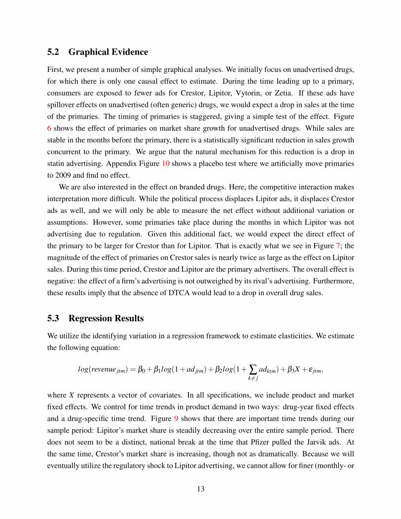
Table 3 presents a regression of the log of the number of statin advertisements for a drug in amarket on the log of the number of political advertisements (in 1000s). The level of observation isa DMA-month for January 2007 until November 2008. We include a variety of fixed effects acrossdifferent specifications. The OLS results show that a 10% increase in political advertising leads toa 1.2% decrease in statin advertising. The effect is slightly larger if you do not account for monthfixed effects. To account for the fact that drug ads cannot be negative, the last columns of Table 3estimates a Tobit model. We find a significantly larger effect: the elasticity of an individual drug’sads with respect to political ads in a market is -0.2598 in our preferred specification, implying thata 10% increase in political ads decreases each drug’s ads by 2.6%. Appendix Table 14 shows theanalogous results using levels instead of logs, with all results strongly negative and significant.
We address four possible concerns about this strategy. First, since the political cycle is knownin advance, firms could have substituted ads to months before or after a market received a largenumber of political ads. In Table, 13 we show that leads and lags of political advertising are notpredictive of drug ads in the current month, indicating that there was not substitution to earlieror later months. Second, firms may substitute from TV advertising to other local media (radio,newspaper) when political ads displace television advertising. In Table 12, we show that totallocal spending is not affected by political ads once local TV ads are controlled for.23 Third, firmsmay modify their detailing plans due to the displacement of their local TV ads by political ads.While we do not have data to directly test for this, discussions with industry managers led us toconclude that this is infeasible, as detailing plans are set at the annual level and cannot be quicklyscaled up or down at the market level. Finally, we do not believe that drug firms are responding topolitical advertising shocks by buying more advertising in less desirable time slots, which wouldcreate measurement error in the number of ads in our data. The relationship between politicaladvertising and drug advertising is largely driven by availability and pre-emption as opposed toprices. The Communications Act of 1934 limits media outlets from raising prices for politicalcampaigns, and Table 15 shows that the price per impression is not changed significantly due topolitical advertising. If firms were shifting their ad buys to lower-priced slots with lower ratings,we would expect a negative relationship.
23The results appear to show that local TV ads and other local media are complements, not substitutes, and isconsistent with the political cycle being a shock to all forms of media in a local market.
12
5.2 Graphical Evidence
First, we present a number of simple graphical analyses. We initially focus on unadvertised drugs,for which there is only one causal effect to estimate. During the time leading up to a primary,consumers are exposed to fewer ads for Crestor, Lipitor, Vytorin, or Zetia. If these ads havespillover effects on unadvertised (often generic) drugs, we would expect a drop in sales at the timeof the primaries. The timing of primaries is staggered, giving a simple test of the effect. Figure6 shows the effect of primaries on market share growth for unadvertised drugs. While sales arestable in the months before the primary, there is a statistically significant reduction in sales growthconcurrent to the primary. We argue that the natural mechanism for this reduction is a drop instatin advertising. Appendix Figure 10 shows a placebo test where we artificially move primariesto 2009 and find no effect.
We are also interested in the effect on branded drugs. Here, the competitive interaction makesinterpretation more difficult. While the political process displaces Lipitor ads, it displaces Crestorads as well, and we will only be able to measure the net effect without additional variation orassumptions. However, some primaries take place during the months in which Lipitor was notadvertising due to regulation. Given this additional fact, we would expect the direct effect ofthe primary to be larger for Crestor than for Lipitor. That is exactly what we see in Figure 7; themagnitude of the effect of primaries on Crestor sales is nearly twice as large as the effect on Lipitorsales. During this time period, Crestor and Lipitor are the primary advertisers. The overall effect isnegative: the effect of a firm’s advertising is not outweighed by its rival’s advertising. Furthermore,these results imply that the absence of DTCA would lead to a drop in overall drug sales.
5.3 Regression Results
We utilize the identifying variation in a regression framework to estimate elasticities. We estimatethe following equation:
log(revenue jtm) = β0 +β1log(1+ad jtm)+β2log(1+ ∑k 6= j
adktm)+β3X + ε jtm,
where X represents a vector of covariates. In all specifications, we include product and marketfixed effects. We control for time trends in product demand in two ways: drug-year fixed effectsand a drug-specific time trend. Figure 9 shows that there are important time trends during oursample period: Lipitor’s market share is steadily decreasing over the entire sample period. Theredoes not seem to be a distinct, national break at the time that Pfizer pulled the Jarvik ads. Atthe same time, Crestor’s market share is increasing, though not as dramatically. Because we willeventually utilize the regulatory shock to Lipitor advertising, we cannot allow for finer (monthly- or
13

quarterly-) product-specific fixed effects. However, we can can allow for a linear, product-specifictime trend that approximates the data reasonably well. In 18, we show that higher order, drug-specific time trends have a negliable effect on the estimates. Because the specification is log-log,we can interpret the coefficients as elasticities.
Table 4 shows the results of OLS specifications for advertised drugs. The first pair of columnsuse contemporaneous ads and revenues; the next pair regresses this month’s revenue on the aver-ages of this month’s and the previous month’s advertising levels; the final pair average the previousthree months’ advertising levels. Previous research has shown that advertising can be cumulativeand/or have a lagged effect (Dubé, Hitsch and Manchanda 2005), but that the effects of DTCAcan depreciate quickly (Jin and Iizuka (2005)). In each regression, the level of analysis is theDMA-month-drug. We include each of the drugs advertised during our sample period from July2007 through November 2008 that are classified in the same in Truven Redbook class 059: Lipitor,Crestor, Vytorin, and Zetia. The dependent variable is logged drug revenue per insured individualin the market. Regardless of controls, the OLS regressions consistently show a small, but statisti-cally significant and positive effect of DTCA on sales. The specifications that allow for a productspecific time trend are typically smaller in magnitude.
We document the causal impact of advertising in Table 5. We instrument own and rival ad-vertising levels using (i) the level of political ads, as well as second- and third-order polynomialsof political ads, (ii) a dummy for the congressional action that halted Lipitor advertising, and (iii)an interaction of this dummy with the polynomials of political advertising. Our instruments areremarkably strong predictors of own and rival advertising. The F-statistic for a test of joint signi-fication of the excluded instruments in the first stage of our main specifications is 493.66 for ownadvertising and 67.30 for rival advertising.
Based on the results in the previous table, the OLS analysis underestimates the effects of ownand rival advertising. The own advertising effect in column 4 (.0064) is less than 10% of theeffect measured in the IV specification (.0764). Similarly, we find substantial evidence of businessstealing in the IV specifications that is absent from the OLS results. As discussed in Section 3,the direction of OLS bias is ambiguous, but in this case it appears that the strategic interactionbetween firms leads to the effect of own advertising being biased downward, while the effect ofrival advertising is biased upward.24
Unsurprisingly, we find that the effects are attenuated as we look at a broader window. The ef-fect of contemporaneous advertising in the drug-year fixed effects regression is the largest (0.0808),while the two-month (0.0764) and three-month (0.0536) moving averages are smaller. Despite this
24One other possible explanation for the bias we find is that measurement error could be attenuating the OLSestimates. Alternatively, we measure a local average treatment effect that captures the short run elasticity of sales withrespect to advertising expenditures and the long run elasticity may be smaller in magnitude.
14

attenuation, the results are stable across specifications. While the estimates that allow for product-specific time trends are smaller in magnitude, we cannot reject that they are statistically the same.We focus on the two-month trailing average specification with drug specific time trends movingforward. Our preferred own-revenue elasticity estimates for advertised drugs is 0.0764, from col-umn 5. This implies that a 10% increase in advertising would yield a 0.76% increase in revenue.Our preferred cross-revenue elasticity estimate is -0.055. Appendix Table 18 shows similar resultsif the outcome of interest is quantity (market share) instead of revenue. These results are consistentwith a model in which advertising is business-stealing and may create an arms race.
Table 6 estimates the spillover effects for unadvertised drugs. Columns 3 and 4 replicate thelast set of specifications in Table 5 in which two-month moving averages of drug advertising arethe independent variables of interest. However, columns 1 and 2 present OLS and IV specificationsin which logged revenue of unadvertised antihyperlipidemia drugs (as classified by Redbook) isthe dependent variable. In the OLS specifications, we find no effect of rival advertising. Once weinstrument for advertising, we find evidence that advertising has a small, but significant spillovereffect. A 10% increase in advertising for the class leads to a 0.23% increase in sales of unadvertiseddrugs. Our results support a model in which advertising has largely persuasive or business-stealingeffects, but also spillovers to unadvertised drugs, consistent with informational effects.
6 Robustness Checks and Heterogeneity
6.1 Robustness Checks
We perform a number of additional analyses and robustness checks. We present three key sets ofspecifications here. First, in Table 17, we explore the direction of the bias in OLS results. Weargue that strategic interaction is an important determinant of returns to advertising. To test this,we run two specifications in which we omit the effect of rival ads. The results are in Columns1 and 3. These specifications explicitly violate our exclusion restriction: shocks to political ad-vertising affect drug sales not only through changes in my own advertising, but changes in myrival’s advertising as well. Therefore, we do not interpret these estimates as causal. When we donot control for rival advertising, the estimated own-advertising elasticity is much smaller (0.0163),less than 15% of the effect measured in columns 2. Both my advertising and my rivals’ advertisingare endogenous and the outcome of dynamic game; our identification strategy allows us to captureboth effects.
Table 18 shows that our results are robust to the different assumptions about the timing ofadvertising effectiveness. Column 2 presents a specification where advertising is measured with aone-month lag, rather than a two-month trailing average. The estimates are quite similar, though
15

larger in magnitude and closer to the contemporaneous estimates in column 2 of Table 5. Thespecification in column 1 controls for the fact that advertising stock might also have an effecton drug revenues by including a one-year lag of advertising as a control. We obtain statisticallyindistinguishable estimates as compared to our preferred specification.
Finally, our identification strategy exploits both the timing of the political process and thepulling of Lipitor ads featuring Dr. Robert Jarvik. We have more confidence in the first source ofidentification; it is possible that the pulling of Lipitor ads also led to numerous news stories andthis publicity, while it contained no content about the quality of the drug itself, may have had animpact on sales. However, in the third column of 18, we still interact the regulatory action withthe level of political advertising and utilize the “intensity of treatment” across areas as a secondinstrument, while omitting the main effect from both stages. We are comparing those states wherea primary would have had a large impact on Lipitor ads if not for the regulatory action with thosestates where a primary affects all drugs more equally. We also run an additional specificationthat includes the main effect of the Jarvik regulatory action and interactions in both stages of theregression and present the results in column 4 Table 18. The estimates are noisier, but confirm ourbasic story. The own advertising elasticity in both of these specifications is larger in magnitudethan our main results, but not statistically different.
6.2 Part D Sample
These results are compelling, but the Truven MarketScan data represent only a fraction of thepotential statin market. While there is no reason to believe the consumers in the Truven MarketScanare not representative of employees of large, self-insured firms, the sample is not representative ofthe population as a whole. In order to further explore the effect of DTCA, we utilize MedicarePart D claims data. Medicare Part D covers a population that is significantly older and sickerthan the Truven MarketScan data. Furthermore, the contractual features of plans do more to alterutilization or steer consumers towards particular drugs. This analysis gives us an opportunity tocompare elasticities across settings and explore additional heterogeneity in the data.
In all our specifications, we aggregate the Part D claims data, which are individual-prescriptionfill level observations, to the DMA-product-month level. We keep only those markets for whichwe have Truven data, leaving us with the same number of observations in each specification andidentical first stage regressions. Any differences in the estimates are due to differences in relativesales across the two samples.
Table 16 shows the results of OLS specifications for advertised drugs. The results are re-markably similar in magnitude to the estimates in Table 4, though slightly larger. The differencesbetween the estimates are rarely statistically significant. In the IV regressions in Table 7, the own
16

advertising elasticities range from 0.054-0.147. while the estimates from the employer-sponsoredsample ranged from 0.076-0.125. In both samples, we see significant evidence of business stealingeffects, though the (negative) effect of rival advertising is smaller in magnitude than the (positive)effect of own advertising. The estimates for the Part D sample are more precise; we cannot rejectthat the estimated elasticities are the same. Replicating our main results in this sample providesadditional confidence in both the qualitative pattern and empirical magnitudes.
The Part D data also allows us to explore heterogeneity in the effect of DTCA across differentdemographic groups, utilization patterns, and insurance regimes. Of primary interest is whetherthese effects are driven by new consumers, with no history of statin use, or by switchers, who maybe more likely to try an alternative statin after seeing an ad. In order to quantify the separate effectson consumers without a history of statin use, we focus on revenue from new prescriptions. Werestrict the claims data to first time prescriptions, defined by the first fill of Crestor, Lipitor, Vytorin,or Zetia. We then collapse the data to the market-month-product level and replicate the sameanalysis. We have slightly fewer observations as we do not observe “new” prescriptions in everyDMA-month-product cell. Otherwise, the specifications are the same as previous specificationsbut utilize a different dependent variable.
The results are presented in Table 8. We report specifications with product specific time trends.There are two key observations. First, the own advertising elasticity is five times as large in mag-nitude for new consumers (0.288 versus 0.054 for the entire sample). Second, the rival elasticitiesare larger in magnitude among new consumers as well (0.149 vs. 0.0401 for the entire sample).We conclude that the effect is largely being driven by new consumers, rather than switchers. Thishas important implications for firm strategy, which we hope to explore in future research.
We also explore additional dimensions of heterogeneity in the appendix. Medicare Part D hasfour phases, corresponding to total spending. What phase a consumer ends the year in reflects boththe marginal cost of drugs to the consumers and their relative utilization. We show that advertisingdoes not have a significant effect on consumption for the sickest consumers - those who end theyear in the “catastrophic coverage” phase of Medicare Part D.25 Finally, consumers can choosebetween two alternative types of insurance plans under the Part D program. They can enroll in astand-alone Part D plan, or a comprehensive Medicare Advantage (MA) plan. The MA plans tendto have more supply-side restrictions, and advertising has a smaller impact among these enrollees.
25The results do not seem to depend on effective marginal prices: the results for the initial coverage phase, inwhich the consumer has a relatively small co-pay, and the donut hole, where they have effectively no coverage, arestatistically the same. This is consistent with previous research that argues that consumers tend to respond to thespot price rather than the true marginal price (Aron-Dine et al. (2014),Abaluck, Gruber and Swanson (2013), Dalton,Gowrisankaran and Town (2014), Einav, Finkelstein and Schrimpf (2014)).
17

7 Implications and Discussion
A back-of-envelope calculation shows that our estimates are quite sensible.26 Lipitor spent $175Mon DTCA in 2009, or $15M a month. US revenue was approximately $490M/month, and theirfinancial statements indicate that costs were 25% of revenue. Our elasticity estimates are 0.0764and 0.0543 for the Truven and Part D samples, respectively. This implies that a 1% increase inadvertising ($150,000) increases revenues net of costs by $200,000-$281,000. While this does notexactly equate marginal costs and marginal revenues, it does hold fixed rival advertising, and sois a partial elasticity. Furthermore, the OLS estimates would imply an increase of revenue net ofcosts by $75,000 assuming our largest estimates. The OLS estimates imply marginal revenue farbelow marginal cost, or that firms are not maximizing profits.
7.1 Simulations
Our results can be used to quantify the magnitudes of business-stealing and spillovers in this mar-ket. In all simulations below, we bootstrap by re-sampling the data set 100 times (with replace-ment), re-estimate our main specifications, and then compute a simulated object such as the changein revenue or quantity. We report the mean of the bootstrapped results, as well as the 95% confi-dence interval.
First, we calculate sales of advertised drugs in the absence of a business-stealing effect ofcompetitor advertising. To do this, we set the coefficient on rival ads equal to zero in the mainspecification (column 4 of 5) and calculate the percentage change in revenue. We do not alter thelevel of the ads themselves. This is important for two reasons. First, firms still benefit from thecontent of their own advertising. Second, we are not measuring an equilibrium outcome; firmsmay choose higher or lower levels of advertising absent a business-stealing effect.
Table 9 presents the results. Panel A shows that business-stealing has a sizable impact onrevenues. Absent the negative impact of rival ads, sales would be 23% higher for Lipitor and 21%higher for Crestor over the sample period.27 To the extent that business-stealing is less likely tobe seen as welfare-enhancing, this has important implications for policy. This also suggests thatDTCA creates a prisoners’ dilemma, where an individual firm has a strong incentive to advertise,but in equilibrium, all are spending more on advertising and seeing minimal effects. Panel Bperforms the same simulation for non-advertised drugs, which effectively eliminates spilloversfrom other drug advertising. In the absence of such spillovers, revenues for unadvertised drugs
26In this calculation, we assume that prices are constant, so that an increase in spending is equivalent to an increasein the number of ads.
27This is a substantial increase, but not unreasonable given our estimates and the data. At $90 for a month’s supply,this amounts to approximately 250 more monthly prescriptions in the average market.
18

would fall by 9.7%. This indicates a potentially large role for welfare-enhancing spillovers in drugadvertising.
We can also quantify the impact that the political process’s shock had on drug firm revenues.We first predict what advertising levels would have been in the absence of any political ads, andthen use our main results to predict revenues in the absence of political ads. Panel A shows thatif the political process had not displaced drug advertising, revenues for Crestor and Lipitor wouldhave been roughly two percent higher over the study period.
Finally, we analyze the impact of changes in the regulatory environment: a ban on DTCA.This eliminates both the effect of a firm’s own ads and their rival’s ads. The FDA is unlikelyto be concerned about firm revenues, and so the outcome of interest is the quantity (share) ofconsumers taking a particular drug. We proceed with our simulations based on the specificationfrom Appendix Table 18. Table 10 shows that all firms see fewer customers under this scenario,although the effect is not identical across drugs. Figure 8 shows the distribution of the percentchange from each simulation for Lipitor, Crestor, and non-advertised drugs. The results show thatin the absence of DTCA, Lipitor is significantly harmed, while Crestor is harmed to a lesser degree.In general, Lipitor advertises more than Crestor during this time period. For non-advertised drugs,we see a more dispersed but still negative effect, as these drugs benefited from rival advertising.
Based on these calculations, we conclude that DTCA is primarily characterized by a business-stealing effect among branded competitors, with a small spillover to unadvertised drugs. Signifi-cantly, DTCA increases the number of patients taking all drugs in the category, advertised or not.We recognize that the statin market has a small number of players that are very close substituteswith few side-effects, and so the empirical effects may differ in other drug classes with a largernumber players or where the “match” of a patient to a drug is more important.
7.2 Discussion
While our results present a consistent story, there are a number of caveats. First, these are short-run elasticities. Though they are much larger for new consumers, the long-run impact is unclear.Second, we do not consider selection into insurance plans or explore the role of physician agency.Given that we are looking at such a short time period, we do not believe these factors bias ourresults. Third, all of our results take the decision to advertise at all as given. This decision innon-random, and our treatment effects need not generalize.
Similarly, some of our results are likely to be specific to the market we study, with a limitednumber of advertisers who are close clinical substitutes. For example, much of the literature hasexamined the antidepressant market, which is similarly characterized by spillovers, but finds littleevidence of business stealing effects (Avery, Eisenberg and Simon (2012); Donohue and Berndt
19

(2004); Narayanan, Desiraju and Chintagunta (2004) and, most recently Shapiro (2014)). Ourresults are consistent with these studies; for example, Shapiro (2014) finds that a cooperative ad-vertising campaign that internalized spillovers would generate five times as many ads and increasecategory size by 13.7%. Our simulations are different in flavor and eliminate ads completely, butfind a 5% reduction in the sales on unadvertised drugs, which comprise the bulk of the market.Here, we argue that substantial advertising expenditure is also defensive and may not provide agreat deal of value from a social perspective, but that eliminating DTCA would significantly re-duce the number of patients taking an effective, safe drug. Our identification strategy is likely to beuseful in a number of product markets, including other drug classes. However, additional variationwill be necessary to separately identify the impact of rival advertising.
A final caution is that these are only partial equilibrium calculations. Firms may alter theirpricing or detailing strategies in response to changes in the competitive environment. Future workshould further explore firm decisions to advertise in an equilibrium model. building on the intuitionin Section 3, we would like to explore a model of advertising competition that can be estimated andused for additional counterfactual calculations. This model should be both tractable and dynamicto capture firm incentives.
8 Conclusion
This paper provides causal estimates of the impact of DTCA. The estimation strategy utilizes ex-ogenous variation in the level of advertising generated by the political cycle. OLS estimates arebiased due to firms strategically advertising in response to both consumer demand and competitoractions. We find significant returns to advertising in the statin market: our estimates indicate that a10% increase in advertising leads to a 0.76% increase in revenues, holding rival actions constant.We estimate the effect in two samples: among the privately insured and among Medicare benefi-ciaries. In the Medicare sample, we show that our effect is primarily driven by new prescriptions.We find both business-stealing and spillover effects of advertising in the statin market.
The impact of DTCA is an empirical question of critical policy importance. Our simulationshighlight the role of advertising competition and the potential for an advertising ban to reducewasteful advertising spending. While sales of unadvertised drugs fall by nearly 5%, the savingsfrom eliminating television advertising are substantial. Our results help quantify the tradeoffsthat policy makers may face when regulating pharmaceutical firms. Furthermore, the impact ofadvertising is a fundamental empirical challenge and our identification strategy provides usefulevidence on this important question.
20

References
Abaluck, Jason, Jonathan Gruber and Ashley T. Swanson. 2013. “A Dynamic Model of Prescrip-tion Drug Utilization.” 2014.
Ackerberg, Daniel A. 2001. “Empirically Distinguishing Informative and Prestige Effects of Ad-vertising.” The RAND Journal of Economics 32(2):316–333.
Aron-Dine, Aviva, Liran Einav, Mark Cullen and Amy Finkelstein. 2014. “Moral Hazard in HealthInsurance: Do Dynamic Incentives Matter?” NBER Working Paper 17802 .
Avery, Rosemary J., Matthew D. Eisenberg and Kosali I. Simon. 2012. “The Impact of Direct-to-Consumer Television and Magazine Advertising on Antidepressant Use.” Journal of Health
Economics 31(5):705–718.
Bagwell, K. 2007. “The Economic Analysis of Advertising.” Handbook of Industrial Organization
3:1701–1844. Mark Armstrong and Rob Porter (eds.).
Berndt, Ernst R. 2005. “To inform or persuade? Direct-to-consumer advertising of prescriptiondrugs.” New England Journal of Medicine 352(4):325–8.
Berndt, Ernst R, Linda T. Bui, David H. Reiley and Glen L. Urban. 1995. “Information, Marketingand Pricing in the U.S. Anti-Ulcer Drug Market.” American Economic Review 85(2):100–105.
Blake, T., C. Nosko and S. Tadelis. 2013. “Consumer Heterogeneity and Paid Search Effectiveness:A Large Scale Field Experiment.”.
Blazing, MA, RP Giugliano, C Cannon, T Musline, A Tershakovec, J White, C Reist, A McCagg,E Braunwald and R Califf. 2014. “Evaluating cardiovascular event reduction with ezetimibeas an adjunct to simvastatin in 18,144 patients after acute coronary syndromes: final baselinecharacteristics of the IMPROVE-IT study population.” American Heart Journal 168(2):205–212.
Bronnenberg, Bart J., Jean-Pierre Dubé, Matthew Gentzkow and Jesse M. Shapiro. 2014. “Dopharmacists buy Bayer? Informed shoppers and the brand premium.” University of Chicagomimeo.
Dafny, Leemore, Kate Ho and Mauricio Varela. 2013. “Let Them Have Choice: Gains fromShifting Away from Employer-Sponsored Health Insurance and toward an Individual Exchange.”American Economic Journal: Economic Policy 5(1):32–58.
21

Dalton, Christina M., Gautam Gowrisankaran and Robert Town. 2014. “Myopia and ComplexDynamic Incentives: Evidence from Medicare Part D.” 2014.
Davidson, Michael and Jennifer Robinson. 2007. “Safety of Aggressive Lipid Management.” Jour-
nal of the American College of Cardiology .
Donohue, Julie M and Ernst R Berndt. 2004. “Effects of Direct-to-Consumer Advertising on Med-ication Choice: The Case of Antidepressants.” Journal of Public Policy & Marketing 23(2):115–127.
Dubé, Jean-Pierre, Günter J Hitsch and Puneet Manchanda. 2005. “An Empirical Model of Adver-tising Dynamics.” Quantitative Marketing and Economics 3(2):107–144.
Duggan, Mark and Fiona Scott Scott Morton. 2010. “The Effect of Medicare Part D on Pharma-ceutical Prices and Utilization.” American Economic Review 100(1):590–607.
Einav, Liran, Amy Finkelstein and Paul Schrimpf. 2014. “The Response of Drug Expenditure toNon-Linear Contract Design: Evidence from Medicare Part D.” 2014.
Faergeman, Ole, L Hill, E Windler, O Wiklund, R Asmar, E Duffield and F Sosef. 2008. “Effi-cacy and Tolerance of rosuvastatin and atorvastatin when force-titrated in patients with primaryhypercholesterolemia: results from the ECLIPSE study.” Cardiology 111(4):219–228.
Gordon, Brett R. and Wesley R. Hartmann. 2013. “Advertising Effects in Presidential Elections.”Marketing Science 32:19–35.
Gordon, Brett R. and Wesley R. Hartmann. 2014. “Advertising Competition in Presidential Elec-tions.” Stanford University mimeo.
Greenland, Philip and Donald Lloyd-Jones. 2008. “Critical Lessons from the ENHANCE Trial.”Journal of the American Medical Association .
Hoelzel, Mark. 2014. “Online Video Advertising is Growing Many Times Faster Than TV, Search,and Most Other Digital Ad Markets.” Business Insider .URL: http://www.businessinsider.com/digital-video-advertising-growth-trends-2014-5
Jack, Andrew. 2009. “The Fall of the World’s Best-Selling Drug.” Financial Times Magazine .URL: http://www.ft.com/intl/cms/s/0/d0f7af5c-d7e6-11de-b578-
00144feabdc0.html?siteedition=intl
Jin, Ginger Zhe and Toshiaki Iizuka. 2005. “The Effects of Prescription Drug Advertising onDoctor Visits.” Journal of Economics & Management Strategy 14(3):701–727.
22

Kolata, Gina. 2014. “Study Finds Alternative to Anti-Cholesterol Drug.” New York Times .URL: http://www.nytimes.com/2014/11/18/health/study-finds-alternative-to-statins-in-
preventing-heart-attacks-and-strokes.html
Lewis, R.A. and J.M. Rao. 2013. “On the near impossibility of measuring the returns to advertis-ing.”.
Mathews, Anna Wilde. 2008. “Congress Investigates Vytorin Ads.” Wall Street Journal .URL: http://blogs.wsj.com/health/2008/01/16/congress-investigates-vytorin-ads/
Moshary, Sarah. 2014. “Price Discrimination across PACs and the Consequences of PoliticalAdvertising Regulation.” MIT Working Paper.
Narayanan, Sridhar, Ramarao Desiraju and Pradeep K. Chintagunta. 2004. “Return on Invest-ment Implications for Pharmaceutical Promotional EExpenditure: The Role of Marketing-MixInteractions.” Journal of Marketing 68(4):90–105.
Rosenthal, M.B., E.R. Berndt, J.M. Donohue, A.M. Epstein and R.G. Frank. 2003. “Demandeffects of recent changes in prescription drug promotion.” Frontiers in Health Policy Research
6(1):1–26.
Shapiro, Brad. 2014. “Positive Spillovers and Free Riding in Advertising of Prescription Pharma-ceuticals: The Case of Antidepressants.” University of Chicago Working Paper.
Spatz, Ian. 2011. “Better Drug Ads, Fewer Side Effects.” New York Times .URL: http://www.nytimes.com/2011/02/10/opinion/10spatz.html
Wosinska, Marta. 2002. “Just What the Patient Ordered? Direct-to-Consumer Advertising and theDemand for Pharmaceutical Products.” Harvard Business School mimeo.
Wosinska, Marta. 2005. “Direct-to-Consumer Advertising and Drug Therapy Compliance.” Jour-
nal of Marketing Research 42(3):323–332.
23

Figures
Figure 2: Political Ad Levels, January-June 2008
Notes: The above maps show a dot for each DMA in the USA. The diameter of each dot isproportional to the number of political ads aired in that market, in that month, for all races(Presidential, Senatorial, House, Gubernatiorial). The first row are January and February; secondrow are March and April, and third row are June and July.
24

Figure 3: National Pharmaceutical Ad Levels for Statins
Notes: The above graphic plots spending on national advertising buys from the Kantar data. Dataspans January 2007-November 2008.
Figure 4: National Pharmaceutical Ad Levels for Statins
Notes: The above graphic plots spending on local advertising buys from the Kantar data. Dataspans January 2007-November 2008. The axes are the same as the previous figure.
25

Figure 5: Political Ads Displace Local Drug Ads, Binned Scatter plot
Notes: The above plots bins of observations from January 2007 to November 2008 at themarket-month level after residualizing by market and year-month fixed effects, and adding backthe sample mean. Twenty bins are used. The fitted line is based on a regression of all underlyingdata, not only the binned values.
Figure 6: Effect of Primaries on Growth in Market Share of Non-Advertised Statins
Note: The above plots estimated coefficients for timing dummies relative to a market’s primarymonth. The dependent variable is the (one-month) change in market share, defined as thepercentage of the population taking a non-advertised statin.
26

Figure 7: Effect of Primaries on Growth in Market Share of Crestor and Lipitor
Note: The above plots estimated coefficients for timing dummies relative to a market’s primarymonth. The dependent variable is the (one-month) change in market share, defined as thepercentage of the population taking Lipitor or Crestor.
27

Figure 8: Simulation Results: Eliminating DTCA
Note: The above plots are histograms of the change in quantity for each drug (or drug group) frombootstrapped simulations that eliminate DTCA from the market over the sample period. Seesection XX for an extended discussion of the methodology.
28

Tables
Table 1: Summary Statistics
Drug Drug Usage (Truven Analysis Data set)Number of Markets 189 Average Branded Share 0.829%Number of Months 17 Range, Branded Share (0.000%, 4.71%)Advertised Statins 4 Average Generic Share 3.05%
Range, Generic Share (0.000%, 7.62%)Political Ads Drug Ads
Average 774 Average Local Ads by Drug 1.56Standard Deviation 1,897 Range, Local Ads (0, 105)
Minimum 0 Average National Ads by Drug 19.71Maximum 22,636 Range, National Ads (0, 145)
Notes: The Truven analysis data set limits the sample to months that are most active in politicaladvertising, July 2007-November 2008. Average Branded Share is by drug, not aggregate for allbrands.
Table 2: Covariate Balance, Part D Data
Below Median Markets Above Median Markets DifferenceAverage Age 71.109 71.309 −0.1994
% Female 0.5489 0.5519 −0.0030% White 0.8536 0.8727 −0.0190% Black 0.0849 0.0933 −0.0083
% Hispanic 0.0147 0.0088 0.0058Mortality Rate 0.0423 0.0425 −0.0002
% LIS 0.6874 0.6657 0.0217∗∗
Notes: We split the Part D beneficiary summary sample into two groups. We take the sum ofpolitical advertising over the 2008 calendar year and compare demographics for markets above andbelow the median. We compare demographics across the two groups. Statistical significance at the10%, 5% and 1% levels are denoted by ∗, ∗∗, and ∗∗∗.
29

Tabl
e3:
Polit
ical
Ads
Dis
plac
eD
rug
Ads
Dep
ende
ntV
aria
ble:
Log
(Loc
alSt
atin
Ads
+1)
,Dru
g-M
arke
t-Y
ear-
Mon
thL
evel
Mod
el:
OL
SO
LS
OL
STo
bit
Tobi
tTo
bit
Log
(Pol
itica
lAds
in10
00s
+1)−
0.18
95∗∗∗−
0.12
08∗∗∗−
0.12
08∗∗∗−
0.84
79∗∗∗−
0.30
97∗∗∗−
0.25
98∗∗∗
(0.0
098)
(0.0
116)
(0.0
116)
(0.0
494)
(0.0
613)
(0.0
103)
Con
trol
s:M
arke
tFE
sX
XX
XX
XY
ear-
Mon
thFE
sX
XX
XD
rug
FEs
XX
XX
XX
Dru
g-Y
ear-
Mon
thFE
sX
XN
24,1
5024,1
5024,1
5024
,150
24,1
5024,1
50R
20.
314
0.36
40.
478
0.30
50.
402
0.55
2N
otes
:Uni
tofo
bser
vatio
nis
the
drug
-mar
ket-
mon
thle
vel.
The
rear
e5
adve
rtis
eddr
ugs,
210
mar
kets
and
23m
onth
sof
data
.OL
San
dTo
bits
tand
ard
erro
rscl
uste
red
atth
em
arke
t-ye
ar-m
onth
leve
l.St
atis
tical
sign
ifica
nce
atth
e10
%,5
%an
d1%
leve
lsar
ede
note
dby∗ ,∗∗
,and∗∗∗ .
Rep
orte
dR
2is
adju
sted
forO
LS,
pseu
dofo
rTob
it.
30

Tabl
e4:
OL
SR
even
ueR
egre
ssio
nsfo
rAdv
ertis
edD
rugs
Dep
ende
ntV
aria
ble:
Log
(Rev
enue
perI
nsur
ed)D
rug-
Mar
ket-
Yea
r-M
onth
Lev
elT
his
Mon
thTw
oM
onth
Trai
ling
Ave
rage
Thr
eeM
onth
Trai
ling
Ave
rage
Ow
nA
ds0.
0194∗∗∗
0.00
64∗∗∗
0.02
39∗∗∗
0.00
66∗∗∗
0.03
16∗∗∗
0.00
86∗∗∗
(0.0
022)
(0.0
020)
(0.0
021)
(0.0
021)
(0.0
020)
(0.0
023)
Riv
alA
ds0.
0042∗
0.00
56∗∗
0.00
160.
0036
0.00
080.
0028
(0.0
025)
(0.0
023)
(0.0
027)
(0.0
026)
(0.0
029)
(0.0
029)
Con
trol
s:M
arke
tFE
sX
XX
XX
XY
earF
Es
XX
XX
XX
Dru
gFE
sX
XX
XX
XD
rug
FE*T
ime
Tren
dX
XX
Dru
g-Y
earF
Es
XX
XN
11,5
5111,5
5111
,550
11,5
5010
,875
10,8
75R
20.
842
0.84
70.
843
0.84
70.
845
0.84
9N
otes
:Reg
ress
ions
are
base
don
the
Truv
enda
ta.S
tand
ard
erro
rscl
uste
red
atth
em
arke
t-ye
ar-m
onth
leve
l.In
clud
esre
venu
esfo
rJul
y20
07un
tilN
ovem
ber2
008.
Adv
ertis
eddr
ugs
are
Cre
stor
,Lip
itor,
Vyt
orin
and
Zet
iadu
ring
this
peri
od.“
Ow
nA
ds”
and
“Riv
alA
ds”
are
cons
truc
ted
asL
og(1
+X).
“Tw
oM
onth
Trai
ling
Ave
rage
”in
dica
tes
that
the
inde
pend
entv
aria
bles
are
cons
truc
ted
asth
eav
erag
eof
the
reve
nue
mon
than
don
em
onth
befo
re.T
he“T
hree
Mon
thTr
ailin
gA
vera
ge”
isco
nstr
ucte
dac
cord
ingl
yus
ing
thre
em
onth
s.Fi
rsts
tage
excl
uded
inst
rum
ents
are
polit
ical
adve
rtis
ing,
itssq
uare
and
cube
,and
inte
ract
ions
with
adu
mm
yth
atta
kes
ona
one
duri
ngA
pril
2008
-Aug
ust2
008.
Stat
istic
alsi
gnifi
canc
eat
the
10%
,5%
and
1%le
vels
are
deno
ted
by∗ ,∗∗
,and∗∗∗ .
31

Tabl
e5:
IVR
even
ueR
egre
ssio
nsfo
rAdv
ertis
edD
rugs
Dep
ende
ntV
aria
ble:
Log
(Rev
enue
perI
nsur
ed)D
rug-
Mar
ket-
Yea
r-M
onth
Lev
elT
his
Mon
thTw
oM
onth
Trai
ling
Ave
rage
Thr
eeM
onth
Trai
ling
Ave
rage
Ow
nA
ds0.
1559∗∗∗
0.08
08∗∗
0.12
52∗∗∗
0.07
64∗∗∗
0.10
48∗∗∗
0.05
36∗∗∗
(0.0
251)
(0.0
344)
(0.0
136)
(0.0
258)
(0.0
099)
(0.0
235)
Riv
alA
ds−
0.10
64∗∗∗−
0.04
92∗∗−
0.09
66∗∗∗
−0.
0548∗∗∗
−0.
0908∗∗∗
−0.
0407∗
(0.0
179)
(0.0
247)
(0.0
112)
(0.0
212)
(0.0
095)
(0.0
230)
Con
trol
s:M
arke
tFE
sX
XX
XX
XY
earF
Es
XX
XX
XX
Dru
gFE
sX
XX
XX
XD
rug
FE*T
ime
Tren
dX
XX
Dru
g-Y
earF
Es
XX
XN
11,5
5111
,551
11,5
5011
,550
10,8
7510,8
75R
20.
755
0.81
90.
788
0.82
40.
810
0.84
0N
otes
:Reg
ress
ions
are
base
don
the
Truv
enda
ta.S
tand
ard
erro
rscl
uste
red
atth
em
arke
t-ye
ar-m
onth
leve
l.In
clud
esre
venu
esfo
rJul
y20
07un
tilN
ovem
ber2
008.
Adv
ertis
eddr
ugs
are
Cre
stor
,Lip
itor,
Vyt
orin
and
Zet
iadu
ring
this
peri
od.“
Ow
nA
ds”
and
“Riv
alA
ds”
are
cons
truc
ted
asL
og(1
+X).
“Tw
oM
onth
Trai
ling
Ave
rage
”in
dica
tes
that
the
inde
pend
entv
aria
bles
are
cons
truc
ted
asth
eav
erag
eof
the
reve
nue
mon
than
don
em
onth
befo
re.T
he“T
hree
Mon
thTr
ailin
gA
vera
ge”
isco
nstr
ucte
dac
cord
ingl
yus
ing
thre
em
onth
s.Fi
rsts
tage
excl
uded
inst
rum
ents
are
polit
ical
adve
rtis
ing,
itssq
uare
and
cube
,and
inte
ract
ions
with
adu
mm
yth
atta
kes
ona
one
duri
ngA
pril
2008
-Aug
ust2
008.
Stat
istic
alsi
gnifi
canc
eat
the
10%
,5%
and
1%le
vels
are
deno
ted
by∗ ,∗∗
,and∗∗∗ .
32

Table 6: Revenue Effect Decomposition
Dependent Variable: Log(Revenue per Insured), Log(Revenue per Insured),Non-Advertised Drugs Advertised Drugs
Model: OLS IV OLS IVOwn Ads - - 0.0239∗∗∗ 0.0764∗∗∗
(0.0021) (0.0258)Rival Ads 0.0018 0.0233∗∗∗ 0.0016 −0.0548∗∗∗
(0.0037) (0.0089) (0.0027) (0.0212)Controls:
Market FEs X X X XDrug FEs and Time Trends X X X XN 3,146 3,146 11,500 11,500R2 0.875 0.874 0.843 0.824Notes: Regressions are based on the Truven data. OLS and IV standard errors clustered at themarket-year-month level. Revenue data are for July 2007 until November 2008. “Own Ads” and“Rival Ads” are constructed as Log(1+X), where X is the two-month trailing average of thenumber of ads. First stage excluded instruments are political advertising, its square and cube, andinteractions with a dummy that takes on a one during April 2008-August 2008. Statisticalsignificance at the 10%, 5% and 1% levels are denoted by ∗, ∗∗, and ∗∗∗.
33

Tabl
e7:
IVR
even
ueR
egre
ssio
nsfo
rAdv
ertis
edD
rugs
,Par
tDD
ata
Dep
ende
ntV
aria
ble:
Log
(Rev
enue
perI
nsur
ed)D
rug-
Mar
ket-
Yea
r-M
onth
Lev
elT
his
Mon
thTw
oM
onth
Trai
ling
Ave
rage
Thr
eeM
onth
Trai
ling
Ave
rage
Ow
nA
ds0.
124∗∗∗
0.03
170.
147∗∗∗
0.05
43∗∗∗
0.12
8∗∗∗
0.04
28∗∗
(0.0
194)
(0.0
242)
(0.0
121)
(0.0
180)
(0.0
0924
)(0.0
184)
Riv
alA
ds−
0.08
67∗∗∗−
0.01
62−
0.11
9∗∗∗
−0.
0401∗∗∗
−0.
118∗∗∗
−0.
0350∗∗
(0.0
140)
(0.0
177)
(0.0
101)
(0.0
151)
(0.0
0892
)(0.0
177)
Con
trol
s:M
arke
tFE
sX
XX
XX
XY
earF
Es
XX
XX
XX
Dru
gFE
sX
XX
XX
XD
rug
FE*T
ime
Tren
dX
XX
Dru
g-Y
earF
Es
XX
XN
11,5
5111
,551
11,5
5011
,550
10,8
7510,8
75R
20.
819
0.87
40.
792
0.86
60.
814
0.87
2N
otes
:Dat
acr
eate
dby
colla
psin
gM
edic
are
Part
Dev
entd
ata
toth
em
arke
t-m
onth
-pro
duct
leve
l.St
anda
rder
rors
clus
tere
dat
the
mar
ket-
year
-mon
thle
vel.
Incl
udes
reve
nues
forJ
uly
2007
until
Nov
embe
r200
8.A
dver
tised
drug
sar
eC
rest
or,L
ipito
r,V
ytor
inan
dZ
etia
duri
ngth
ispe
riod
.“O
wn
Ads
”an
d“R
ival
Ads
”ar
eco
nstr
ucte
das
Log
(1+X
).“T
wo
Mon
thTr
ailin
gA
vera
ge”
indi
cate
sth
atth
ein
depe
nden
tvar
iabl
esar
eco
nstr
ucte
das
the
aver
age
ofth
ere
venu
em
onth
and
one
mon
thbe
fore
.The
“Thr
eeM
onth
Trai
ling
Ave
rage
”is
cons
truc
ted
acco
rdin
gly
usin
gth
ree
mon
ths.
Firs
tst
age
excl
uded
inst
rum
ents
are
polit
ical
adve
rtis
ing,
itssq
uare
and
cube
,and
inte
ract
ions
with
adu
mm
yth
atta
kes
ona
one
duri
ngA
pril
2008
-Aug
ust2
008.
Stat
istic
alsi
gnifi
canc
eat
the
10%
,5%
and
1%le
vels
are
deno
ted
by∗ ,∗∗
,and∗∗∗ .
34

Tabl
e8:
IVR
even
ueR
egre
ssio
nfo
rFir
stPr
escr
iptio
nsO
nly,
Part
DD
ata
Dep
ende
ntV
aria
ble:
Log
(Rev
enue
perI
nsur
ed)D
rug-
Mar
ket-
Yea
r-M
onth
Lev
elT
his
Mon
thTw
oM
onth
Trai
ling
Ave
rage
Thr
eeM
onth
Trai
ling
Ave
rage
Mod
el:
OL
SIV
OL
SIV
OL
SIV
Ow
nA
ds0.
0496∗∗∗
0.36
1∗∗∗
0.04
69∗∗∗
0.28
8∗∗∗
0.04
72∗∗∗
0.25
5∗∗∗
(0.0
0408
)(0.0
973)
(0.0
0418
)(0.0
769)
(0.0
0467
)(0.0
800)
Riv
alA
ds0.
0528∗∗∗−
0.17
3∗∗
0.05
11∗∗∗
−0.
149∗∗
0.04
97∗∗∗
−0.
134∗
(0.0
0531
)(0.0
743)
(0.0
0577
)(0.0
667)
(0.0
0631
)(0.0
788)
Con
trol
s:M
arke
tFE
sX
XX
XX
XY
earF
Es
XX
XX
XX
Dru
gFE
sX
XX
XX
XD
rug
FE*T
ime
Tren
dX
XX
XX
XN
10,7
8910
,789
10,7
8810
,788
10,1
2510,1
25R
20.
594
0.29
10.
593
0.42
10.
591
0.48
0N
otes
:Dat
acr
eate
dby
rest
rict
ing
even
tdat
ato
first
pres
crip
tions
only
and
colla
psin
gto
the
mar
ket-
mon
th-p
rodu
ctle
vel.
Stan
dard
erro
rscl
uste
red
atth
em
arke
t-ye
ar-m
onth
leve
l.In
clud
esre
venu
esfo
rJul
y20
07un
tilN
ovem
ber2
008.
Adv
ertis
eddr
ugs
are
Cre
stor
,Lip
itor,
Vyt
orin
and
Zet
iadu
ring
this
peri
od.“
Ow
nA
ds”
and
“Riv
alA
ds”
are
cons
truc
ted
asL
og(1
+X).
“Tw
oM
onth
Trai
ling
Ave
rage
”in
dica
tes
that
the
inde
pend
entv
aria
bles
are
cons
truc
ted
asth
eav
erag
eof
the
reve
nue
mon
than
don
em
onth
befo
re.T
he“T
hree
Mon
thTr
ailin
gA
vera
ge”
isco
nstr
ucte
dac
cord
ingl
yus
ing
thre
em
onth
s.Fi
rsts
tage
excl
uded
inst
rum
ents
are
polit
ical
adve
rtis
ing,
itssq
uare
and
cube
.Sta
tistic
alsi
gnifi
canc
eat
the
10%
,5%
and
1%le
vels
are
deno
ted
by∗ ,∗∗
,and∗∗∗ .
35

Table 9: Revenue Simulations
Panel A: Simulations for Advertised Drugs% Change in Revenue: Crestor Lipitor
(1) Eliminating Business-Stealing 0.2107 0.2327Confidence Interval (0.0047, 0.5639) (0.0054, 0.6082)
(2) Eliminate Political Ads 0.0207 0.0163Confidence Interval (0.0039, 0.0689) (0.0038, 0.0484)
Panel B: Simulations for Non-Advertised Drugs% Change in Revenue: Unadvertised Drugs
(3) Eliminate Spillovers −0.0974Confidence Interval (−0.1539,−0.0262)
(4) Eliminate Political Ads −0.0030Confidence Interval (−0.0049,−0.0008)
Notes: Estimates from “Two Month Trailing Average” and drug-specific time trend specificationsare used in all simulations. (1) sets the coefficient on rival advertising in column 4 of Table 5 equalto zero. (2) estimates the number of drug ads in the absence of political ads, and then estimatessales at those levels of advertising. In Panel B, (3) sets the coefficient on rival advertising incolumn 2 of Table 6 equal to zero. (4) estimates the number of drug ads in the absence of politicalads, and then estimates sales for non-advertised drugs at those levels of advertising. Estimates arebootstrapped by re-sampling the data set, re-estimating the primary specifications, andre-computing the counterfactual exercise on the observed data. We use 100 bootstrap replicationsand report the 2.5%-97.5% confidence interval as well as then mean.
Table 10: Quantity Simulations
% Change in Quantity Crestor Lipitor Unadvertised(1) Ban All Advertising −0.0094 −0.0255 −0.0491
Confidence Interval (−0.0444, 0.0248) (−0.0614, 0.0070) (−0.1230, 0.0107)
Notes: Estimates from “Two Month Trailing Average” and drug-specific time trend specificationsare used in all simulations. The dependent variable is the log of the market share of a product. Thesimulation sets the coefficient on own and rival advertising equal to zero. Estimates arebootstrapped by re-sampling the data set, re-estimating the primary specifications, andre-computing the counterfactual exercise on the observed data. We use 100 bootstrap replicationsand report the 2.5%-97.5% confidence interval as well as then mean. Figure 8 shows thedistributions of the simulated outcomes.
36

Appendix
Supplemental Appendix For Online Publication
A Model Assumptions and Simulation Details
Assumption 1. Function D j is smooth and continuous in all its arguments; first- and second-
derivatives are defined everywhere. Function D j is concave in all arguments.
Note that Logit demand satisfies this assumption, as do many other standard demand formula-tions. Concavity gives the result that rival advertising lowers the return to own advertising underspillovers, and raises it under business-stealing.
Assumption 2. The following conditions hold: ∂D j∂a j
> 0 and ∂D j∂a j a j=0
∣∣∣∣> cρ
.
Assumption 2 guaratees there is an incentive to advertise. If a firm’s advertising createsspillovers for rivals, that implies that ∂D j
∂a− j> 0 in our notation, while business-stealing implies
∂D j∂a− j
< 0. When we say that the effectiveness of advertising is diminishing in the level of drug
demand, we mean that ∂D j²∂a j∂ξ j
< 0, while if it is complementary to the level of drug demand we
have ∂D j²∂a j∂ξ j
> 0. A firm’s first-order condition for advertising is satisfied when ∂D j∂a j
= cρ
.Parameters were set to the following values: α1 = α2 = 0, c = 1, ρ = 1000. Matlab’s FSOLVE
function was used to set a system of first-order conditions to zero. We use 200 markets and wedraw values of ξ for each firm in each market where ξ ∼ N(0,0.25).
Analytic values of own and rival advertising elasticities are calculated as the mean over allobservations of
ηown = β1(1− s j)−β2s− j
ηrival = β2(1− s j)−β1s− j
We drop any simulations where Matlab’s FSOLVE function failed to converge to a solutionfor firm first-order conditions for advertising levels. The full space of simulations covered β1 ∈[0.01,0.3] and β2 ∈ [−0.4,−0.01], both in increments of 0.005. The share of simulations where thebias in estimating own advertising elasticity was less than 5%, was only 1.54% of simulations, and1.20% for rival advertising elasticity. The table below shows for one particular set of parametervalues the OLS bias in estimating elasticities of own and rival ads.
37

Table 11: Sample Model Simulation Results
Dependent Variable: Log(Revenue)Specification: Naive With ξ Analytic Values
(1) (2) (3)Log(1+Own Ads) 0.0945∗∗∗ 0.1457∗∗∗ 0.1497
(0.0263) (0.0020)Log(1+Rival Ads) −0.0286 −0.2641∗∗∗ −0.2516
(0.0238) (0.0017)Control: ξ XN 200 200R2 0.267 0.998
Notes: Parameter values for these results were β1 = 0.1 and β2 =−0.3. Firm optimal advertisinglevels were solved for using Matlab’s FSOLVE routine and first-order conditions for profitmaximization. Estimates are for equation 1, with ξ j and ξ− j as additional controls in the secondcolumn.
B Additional Robustness Checks
Figure 9: Time Trends
Notes: The above graphic plots the share of Lipitor and Crestor from the Truven data as apercentage of total statin sales over the period of January 2007-November 2008. Note differentaxes.
38

Figure 10: Effect of Placebo Primaries on Shares of Non-Advertised Sales
Note: The above plots estimated coefficients for timing dummies relative to a market’s primarymonth, with the “timing” of the primary shifted 12 months forward. The dependent variable is the(one-month) change in market share, defined as the percentage of the population taking anon-advertised statin.
Table 12: Robustness: No Substitution to Other Media
Dependent Variable: Local Non-TV AdvertisingSpending, Product-Market-Year-Month Level
Model: OLS OLS OLSPolitical Ads (1000s) −0.4474∗∗ −0.2477 −0.2802
(0.1830) (0.1843) (0.1849)Local TV Drug Ads 1.0554∗∗∗ 1.1303∗∗∗
(0.1357) (0.1379)National TV Drug Ads −0.0867∗∗∗
(0.0125)Controls:
Market FEs X X XYear-Month FEs X X XDrug FEs X X XN 20,087 20,087 20,087R2 0.080 0.100 0.101
Notes: Regressions combine the Wisconsin and Kantar data sets. OLS standard errors clustered atthe market-year-month level. Results differ from Table 3 as this is at the individual drug level.Statistical significance at the 10%, 5% and 1% levels are denoted by ∗, ∗∗, and ∗∗∗.
39

Table 13: Robustness: No Substitution to Earlier/Later Months
Dependent Variable: Local Drug Ads,Product-Market-Year-Month Level
Model: OLS OLS OLS OLSPolitical Ads (1000s) −0.0819∗∗∗ −0.0632∗∗
(0.0263) (0.0304)One Month Lag 0.0265 0.0012
(0.0284) (0.0299)One Month Lead −0.0239 -0.0405
(0.0301) (0.0294)Controls:
Market FEs X X X XYear-Month FEs X X X XDrug FEs X X X XDrug National Ads X X X XN 8,925 8,925 8,120 8,120R2 0.225 0.225 0.219 0.218
Notes: Regressions combine the Wisconsin and Kantar data sets. OLS standard errors clustered atthe market-year-month level. Results differ from Table 3 as this is at the individual drug level.Statistical significance at the 10%, 5% and 1% levels are denoted by ∗, ∗∗, and ∗∗∗.
Table 17: Effect of Business Stealing (IV Results)
Dependent Variable: Log(Revenue per Insured)
Exposure: 2-Month 3-Month
(1) (2) (3) (4)
Log Own Ads 0.0121∗∗∗ 0.0764∗∗∗ 0.0119∗∗∗ 0.0536∗∗∗
(0.0022) (0.0258) (0.0026) (0.0235)Log Rival Ads −0.0548∗∗∗ −0.0407∗
(0.0212) (0.0230)
ControlsMarket FE X X X XDrug FEs and Time Trends X X X X
N 11,550 11,550 10,875 10,875R2 0.847 0.824 0.849 0.840
Notes: Standard errors clustered at the market-year-month level. Revenue data are for July 2007until November 2008. “Own Ads” and “Rival Ads” are constructed as Log(1+X), where X is atrailing average of the number of ads. T-statistics in parentheses. First stage excluded instrumentsare political advertising, its square and cube, and interactions with a dummy that takes on a oneduring April 2008-August 2008. Statistical significance at the 10%, 5% and 1% levels are denotedby ∗, ∗∗, and ∗∗∗.
40
Tabl
e14
:Pol
itica
lAds
Dis
plac
eD
rug
Ads
Dep
ende
ntV
aria
ble:
Stat
inA
ds,D
rug-
Mar
ket-
Yea
r-M
onth
Lev
elM
odel
:O
LS
OL
SO
LS
Tobi
tTo
bit
Tobi
tPo
litic
alA
ds(1
000s
)−
0.29
03∗∗∗−
0.22
57∗∗∗−
0.22
57∗∗∗−
1.54
84∗∗∗−
0.84
38∗∗∗−
0.92
57∗∗∗
(0.0
212)
(0.0
216)
(0.0
217)
(0.1
271)
(0.1
084)
(0.0
239)
Con
trol
s:M
arke
tFE
sX
XX
XX
XY
ear-
Mon
thFE
sX
XX
XD
rug
FEs
XX
XX
XX
Dru
g-Y
ear-
Mon
thFE
sX
XN
24,1
5024,1
5024,1
5024
,150
24,1
5024,1
50R
20.
226
0.25
80.
374
0.19
80.
254
0.33
7N
otes
:Reg
ress
ions
com
bine
the
Wis
cons
inan
dK
anta
rdat
ase
ts.U
nito
fobs
erva
tion
isth
edr
ug-m
arke
t-m
onth
leve
l.O
LS
and
Tobi
tsta
ndar
der
rors
clus
tere
dat
the
mar
ket-
year
-mon
thle
vel.
Stat
istic
alsi
gnifi
canc
eat
the
10%
,5%
and
1%le
vels
are
deno
ted
by∗ ,∗∗
,and∗∗∗ .
41

Tabl
e15
:Pol
itica
lAds
and
Ad
Pric
ing
Dep
ende
ntV
aria
ble:
Cos
tper
Uni
tofD
rug
Adv
ertis
ing
Polit
ical
Ads
(100
0s)
0.00
290.
0037
0.00
230.
0012
(0.0
059)
(0.0
051)
(0.0
064)
(0.0
063)
Con
trol
s:M
arke
tFE
sX
XX
Mon
thFE
sX
XD
rug
FEs
XN
2584
2584
2584
2584
R2
0.00
00.
578
0.61
00.
634
Not
es:R
egre
ssio
nsco
mbi
neth
eW
isco
nsin
and
Kan
tard
ata
sets
.Uni
tofo
bser
vatio
nis
the
drug
-mar
ket-
mon
thle
vel.
Stan
dard
erro
rscl
uste
red
atth
em
arke
t-ye
ar-m
onth
leve
l.St
atis
tical
sign
ifica
nce
atth
e10
%,5
%an
d1%
leve
lsar
ede
note
dby∗ ,∗∗
,and∗∗∗ .
42

Tabl
e16
:OL
SR
even
ueR
egre
ssio
nsfo
rAdv
ertis
edD
rugs
,Par
tDD
ata
Dep
ende
ntV
aria
ble:
Log
(Rev
enue
perI
nsur
ed)D
rug-
Mar
ket-
Yea
r-M
onth
Lev
elT
his
Mon
thTw
oM
onth
Trai
ling
Ave
rage
Thr
eeM
onth
Trai
ling
Ave
rage
Ow
nA
ds0.
0229∗∗∗
0.00
991∗∗∗
0.02
59∗∗∗
0.00
817∗∗∗
0.03
24∗∗∗
0.00
792∗∗∗
(0.0
0215
)(0.0
0186
)(0.0
0197
)(0.0
0192
)(0.0
0192
)(0.0
0208
)R
ival
Ads
0.00
457∗∗
0.00
692∗∗∗
0.00
0423
0.00
206
−0.
0003
830.
0004
53(0.0
0200
)(0.0
0187
)(0.0
0217
)(0.0
0209
)(0.0
0238
)(0.0
0235
)C
ontr
ols:
Mar
ketF
Es
XX
XX
XX
Yea
rFE
sX
XX
XX
XD
rug
FEs
XX
XX
XX
Dru
gFE
*Tim
eTr
end
XX
XD
rug-
Yea
rFE
sX
XX
N11,5
5111
,551
11,5
5011
,550
10,8
7510,8
75R
20.
871
0.87
70.
871
0.87
70.
873
0.87
8N
otes
:Dat
acr
eate
dby
colla
psin
gM
edic
are
Part
Dev
entd
ata
toth
em
arke
t-m
onth
-pro
duct
leve
l.O
LS
and
IVst
anda
rder
rors
clus
tere
dat
the
mar
ket-
year
-mon
thle
vel.
Incl
udes
reve
nues
forJ
uly
2007
until
Nov
embe
r200
8.A
dver
tised
drug
sar
eC
rest
or,L
ipito
r,V
ytor
inan
dZ
etia
duri
ngth
ispe
riod
.“O
wn
Ads
”an
d“R
ival
Ads
”ar
eco
nstr
ucte
das
Log
(1+X
).“T
wo
Mon
thTr
ailin
gA
vera
ge”
indi
cate
sth
atth
ein
depe
nden
tvar
iabl
esar
eco
nstr
ucte
das
the
aver
age
ofth
ere
venu
em
onth
and
one
mon
thbe
fore
.The
“Thr
eeM
onth
Trai
ling
Ave
rage
”is
cons
truc
ted
acco
rdin
gly
usin
gth
ree
mon
ths.
Firs
tsta
geex
clud
edin
stru
men
tsar
epo
litic
alad
vert
isin
g,its
squa
rean
dcu
be,a
ndin
tera
ctio
nsw
itha
dum
my
that
take
son
aon
edu
ring
Apr
il20
08-A
ugus
t200
8.St
atis
tical
sign
ifica
nce
atth
e10
%,5
%an
d1%
leve
lsar
ede
note
dby∗ ,∗∗
,and∗∗∗ .
43

Table 19: Heterogeneity, Part D Data
Dependent Variable: Log(Revenue per Insured)Two-Month Trailing Average Three-Month Trailing Average
OLS IV OLS IVPanel A: Beneficiaries Ending Year in Initial Coverage Phase
Log Own Ads 0.0347∗∗∗ 0.221∗∗∗ 0.0437∗∗∗ 0.186∗∗∗
(0.00219) (0.0177) (0.00215) (0.0132)Log Rival Ads 0.00883∗∗∗ −0.166∗∗∗ 0.00908∗∗∗ −0.157∗∗∗
(0.00275) (0.0148) (0.00300) (0.0129)N 11,550 11,550 10,875 10,875R2 0.842 0.682 0.845 0.735
Panel A: Beneficiaries Ending Year in Donut HoleLog Own Ads 0.0212*** 0.203*** 0.0273*** 0.184***
(0.00238) (0.0181) (0.00235) (0.0143)Log Rival Ads −0.00875*** −0.186*** −0.00922*** −0.194***
(0.00287) (0.0151) (0.00312) (0.0139)N 11,547 11,547 10,872 10,872R2 0.824 0.666 0.825 0.691
Panel A: Beneficiaries Ending Year in the Catastrophic PhaseLog Own Ads 0.0135*** −0.0128 0.0149*** 0.000359
(0.00260) (0.0164) (0.00260) (0.0129)Log Rival Ads −0.00290 0.0100 −0.00766** −0.00157
(0.00323) (0.0140) (0.00351) (0.0130)N 11,491 11,491 10,819 10,819R2 0.795 0.793 0.796 0.795
Notes: Data created by restricting event data to beneficiaries ending the year in each phase andcollapsing to the market-month-product level. OLS and IV standard errors clustered at themarket-year-month level. Includes revenues for July 2007 until November 2008. Advertised drugsare Crestor, Lipitor, Vytorin and Zetia during this period. “Own Ads” and “Rival Ads” areconstructed as Log(1+X). “Two Month Trailing Average” indicates that the independent variablesare constructed as the average of the revenue month and one month before. The “Three MonthTrailing Average” is constructed accordingly using three months. First stage excluded instrumentsare political advertising, its square and cube. All regressions include market, year, and drug fixedeffects and a drug specific time trend. Statistical significance at the 10%, 5% and 1% levels aredenoted by ∗, ∗∗, and ∗∗∗.
44

Tabl
e18
:Rob
ustn
ess
Che
cks
(IV
Res
ults
)
Dep
ende
ntV
aria
ble:
Dep
ende
ntV
aria
ble:
Log
(Rev
enue
perI
nsur
ed)
Log
(Day
sSu
pply
perI
nsur
ed)
Ow
nA
ds(2
-Mon
thTr
ailin
g)0.
766∗∗∗
0.13
06∗∗∗
0.11
89∗∗
0.07
34**
*0.
1495∗∗∗
0.06
57∗∗∗
(0.0
258)
(0.0
492)
(0.0
549)
(0.0
270)
(0.0
141)
(0.0
255)
Riv
alA
ds(2
-Mon
thTr
ailin
g)−
0.05
50∗∗∗
−0.
0958∗∗−
0.09
15∗∗
-0.0
425*
*−
0.12
02∗∗∗
−0.
0488∗∗
(0.0
212)
(0.0
383)
(0.0
451)
(0.0
215)
(0.0
116)
(0.0
209)
Jan.
-Jun
.’07
Ads
0.06
99∗∗
(0.0
322)
1-M
onth
Lag
ged
Ow
nA
ds0.
1444∗∗∗
(0.0
466)
1-M
onth
Lag
ged
Riv
alA
ds−
0.10
41∗∗∗
(0.0
365)
Mar
ketF
Es
XX
XX
XX
XY
earF
Es
XX
XX
XX
XD
rug
FEs
XX
XX
XX
XD
rug
FE*T
ime
Tren
dX
XX
XX
XD
rug
FE*T
ime
Tren
d^2
XD
rug-
Yea
rFE
sX
1(FD
A),
infir
stst
age
XX
XX
XX
1(FD
A),
inse
cond
stag
eX
N11,5
5111,5
5111
,550
11,5
5011
,550
11,5
5011,5
50R
20.
871
0.87
70.
776
0.78
70.
832
0.74
50.
822
Not
es:D
ata
crea
ted
byco
llaps
ing
Med
icar
ePa
rtD
even
tdat
ato
the
mar
ket-
mon
th-p
rodu
ctle
vel.
Stan
dard
erro
rscl
uste
red
atth
em
arke
t-ye
ar-m
onth
leve
l.In
clud
esre
venu
esfo
rJul
y20
07un
tilN
ovem
ber2
008.
Adv
ertis
eddr
ugs
are
Cre
stor
,Lip
itor,
Vyt
orin
and
Zet
iadu
ring
this
peri
od.“
Ow
nA
ds”
and
“Riv
alA
ds”
are
cons
truc
ted
asL
og(1
+X).
“Tw
oM
onth
Trai
ling
Ave
rage
”in
dica
tes
that
the
inde
pend
entv
aria
bles
are
cons
truc
ted
asth
eav
erag
eof
the
reve
nue
mon
than
don
em
onth
befo
re.T
he“T
hree
Mon
thTr
ailin
gA
vera
ge”
isco
nstr
ucte
dac
cord
ingl
yus
ing
thre
em
onth
s.Fi
rst
stag
eex
clud
edin
stru
men
tsar
epo
litic
alad
vert
isin
g,its
squa
rean
dcu
be,a
ndin
tera
ctio
nsw
itha
dum
my
that
take
son
aon
edu
ring
Apr
il20
08-A
ugus
t200
8.St
atis
tical
sign
ifica
nce
atth
e10
%,5
%an
d1%
leve
lsar
ede
note
dby∗ ,∗∗
,and∗∗∗ .
45

Table 20: Heterogeneity II, Part D Data
Dependent Variable: Log(Revenue per Insured)Two-Month Trailing Average Three-Month Trailing Average
OLS IV OLS IVPanel A: Beneficiaries in MA Plans
Log Own Ads 0.0203∗∗∗∗ 0.106∗∗∗ 0.0271∗∗∗ 0.0963∗∗∗
(0.00345) (0.0219) (0.00344) (0.0172)Log Rival Ads −0.00876∗∗ −0.0994∗∗∗ −0.0118∗∗ −0.104∗∗∗
(0.00445) (0.0191) (0.00482) (0.0177)N 10,996 10,996 10,364 10,364R2 0.813 0.795 0.814 0.800
Panel A: Beneficiaries in Stand-alone Part D PlansLog Own Ads 0.0267∗∗∗ 0.167∗∗∗ 0.0330∗∗∗ 0.143∗∗∗
(0.00192) (0.0128) (0.00186) (0.00975)Log Rival Ads 0.00295 −0.134∗∗∗ 0.00251 −0.130∗∗∗
(0.00215) (0.0107) (0.00236) (0.00935)N 11,550 11,550 10,875 10,875R2 0.893 0.800 0.894 0.826...Panel C: LIS-Eligible Beneficiaries OnlyLog Own Ads 0.0207∗∗∗ 0.0348∗∗∗ 0.0241∗∗∗ 0.0379∗∗∗
(0.00231) (0.0121) (0.00227) (0.00907)Log Rival Ads 0.00252 −0.0223∗∗ −0.000817 −0.0288∗∗∗
(0.00260) (0.0102) (0.00287) (0.00911)N 11,538 11,538 10,863 10,863R2 0.858 0.856 0.858 0.857
Notes: Data created by restricting event data to beneficiaries ending the year in each plan type andcollapsing to the market-month-product level. OLS and IV standard errors clustered at themarket-year-month level. Includes revenues for July 2007 until November 2008. Advertised drugsare Crestor, Lipitor, Vytorin and Zetia during this period. “Own Ads” and “Rival Ads” areconstructed as Log(1+X). “Two Month Trailing Average” indicates that the independent variablesare constructed as the average of the revenue month and one month before. The “Three MonthTrailing Average” is constructed accordingly using three months. First stage excluded instrumentsare political advertising, its square and cube. All regressions include market, year, and drug fixedeffects and a drug specific time trend. Statistical significance at the 10%, 5% and 1% levels aredenoted by ∗, ∗∗, and ∗∗∗.
46