Import tariffs and export subsidies in the World Trade Organization:

A small-country approach

By Tanapong Potipiti

No. 119/September 2012

ARTNeT Working Paper Series

Asia-Pacific Researchand Training Network on Trade

© ARTNeT 2012

The ARTNeT Working Paper Series disseminates the findings of work in progress to encourage the exchange of ideas about trade issues. An objective of the series is to get the findings out quickly, even if the presentations are less than fully polished. ARTNeT working papers are available online at www.artnetontrade.org. All material in the working papers may be freely quoted or reprinted, but acknowledgment is requested, together with a copy of the publication containing the quotation or reprint. The use of the working papers for any commercial purpose, including resale, is prohibited. Asia-Pacific Research and Training Network on Trade (ARTNeT) is an open regional network of research and academic institutions specializing in international trade policy and facilitation issues. IDRC, UNCTAD, UNDP, ESCAP and the WTO, as core network partners, provide substantive and/or financial support to the network. The Trade and Investment Division of ESCAP, the regional branch of the United Nations for Asia and the Pacific, provides the Secretariat of the network and a direct regional link to trade policymakers and other international organizations. Disclaimer: The opinion, figures and estimates are the responsibility of the authors and should not be considered as reflecting the views or carrying the approval of the United Nations, ARTNeT members, partners or authors’ employers.

ARTNeT Working Paper Series

No. 119/September 2012

Import tariffs and export subsidies in the World Trade Organization:

A small-country approach

By Tanapong Potipiti

Tanapong Potipiti, is a Lecturer in Economics at Chulalongkorn University, Bangkok, Thailand. The author is grateful to Robert Staiger, Yeon-Cho Che, John Kennan, Bijit Bora, Kiriya Kulkolkarn and the partic¬ipants in the WTO seminar for their helpful comments. The author also thanks WTO for its financial support. The opinion, figures, and estimates are the responsibility of the authors and should not be considered as reflecting the views or carrying the approval of the United Nations. Any remaining errors are the responsibility of the author, who can be contacted by e-mail at Tanapong.P@chula.ac.th .

Please cite this paper as: Potipiti, Tanapong, 2012. Import tariffs and export subsidies in the World Trade Organization: A small – country approach. ARTNeT Working Paper No. 119, September, Bangkok, ESCAP. Available from www.artnetontrade.org.

Contents

1. Introduction .........................................................................................................................................6

2. Basic story ............................................................................................................................................8

3. Basic model ..........................................................................................................................................9

4. Import tariffs, export subsidies and trade agreements ................................................................15

5. Conclusion..........................................................................................................................................27

References ...................................................................................................................................................28

5

Import tariffs and export subsidies in the World Trade Organization:

A small-country approach

Tanapong Potipiti

Abstract

This paper develops a simple small-country model to explain why the World Trade

Organization (WTO) prohibits export subsidies but allows import tariffs. Governments choose

protection rates (import tariffs/export subsidies) to maximize a weighted sum of social welfare

and lobbying contributions. While transportation costs decrease due to the progress of trade

liberalization and lower transportation costs, import-competing sectors decline but export

industries grow. In the growing export industries, the surplus generated by protection is eroded

by new entrants. Therefore, the rent that governments gain from protecting the export sectors

by using export subsidies is small. On the other hand, in the import-competing sectors, capital

is sunk and no new entrants erode the protection rent. Therefore, governments can get large

political contributions from protecting these import-competing sectors. This paper shows that

under fast capital mobility, governments with a high bargaining power are better off than with a

trade agreement that allows import tariffs but prohibits export subsidies.

JEL code: F13, F53

Key words: Export subsidy agreement, import tariff, WTO

6

1. Introduction

Since 1948, GATT Article XVI has called for contracting parties to avoid export sub-

sidies on primary products and to abolish export subsidies on other goods. The WTO

Agreement on Subsidies and Countervailing Measures built on the Tokyo Round subsidies

code (issued in 1979) defines export subsides and prohibits them on non-primary products. As

pointed out by Bagwell and Staiger (2001), the prohibition of export subsidies presents a puzzle

to trade economists; it contradicts predictions made by the standard theories of trade

agreements which find that the role of a trade agreement is to solve the prisoner's dilemma

problem driven by terms-of-trade externalities.1In the non-cooperative equilibrium, large

countries exploit their market power to maximize their welfare by using import tariffs and

export taxes to decrease the prices of imports and increase the prices of exports. As a result,

import tariffs and export taxes are higher than their efficient levels, and the volume of trade is

less than its efficient level. These countries can improve their welfare if they agree to decrease

import tariffs and export taxes, thereby promoting trade.

The standard theories fail to explain why governments use export subsidies policies in

the absence of a trade agreement. According to the standard theories, governments lose their

terms of trade and national income by employing export subsidies. The standard terms-of-trade

theories thus fail to even rationalize the use of export subsidies. A way to solve this puzzle is to

allow governments to be motivated by both national income and distributional concerns. If a

government is highly concerned with the welfare of its exporting sectors, that government will

choose export subsidies. This approach has the following implication: when a government

subsidizes exports, the world price of the export good falls and foreign consumers receive a

positive externality from the subsidy policy. Under a cooperative trade agreement, this positive

externality is internalized, encouraging export subsidies. However, this result contradicts the

WTO rule prohibiting export subsidies.

Another relevant strand of literature concerns strategic trade policy. In the seminal

paper by Brander and Spencer (1985), export sectors compete in a Cournot fashion within a

model with two large exporting countries and one importing country. Export sectors compete in

a Cournot fashion. They show that in the non-cooperative equilibrium export subsidies are

optimal for governments of the exporting countries. However, the welfare of the two exporting

countries improves when both agree to limit export subsidies. Bagwell and Staiger (2001)

studied a model similar to that given in Brander and Spencer (1985) in a standard

partial-equilibrium setting; they found the same result under the condition that exporting

governments' political concerns weighed heavily on producer surplus. Furthermore, they

showed that although an exporting government gained when limiting export subsidies, the

1 Among the representatives of the standard theories are: Johnson, 1954; Grossman and Helpman, 1995; Levy, 1999; and Bagwell and Staiger, 1999.

7

outcome was inefficient from a global perspective. In the efficient outcome, export subsidies

should be promoted and the importing country should transfer income to the exporting

countries.

The studies discussed above are based on large-country models. Trade agreements are

instruments to solve externality problems among the governments of large countries. Another

strand of literature argues that trade agreements can be used as a commitment device to help a

government enhance its credibility and solve domestic time-inconsistency problems (see, for

example, Staiger and Tabellini, 1987, Tornell, 1991, Maggi and Rodriguiez-Clare, 1998, and

Mitra, 2002). These models provide a rationale for the government of a small country to

commit to a free trade agreement and to eliminate tariffs and export subsidies.

Maggi and Rodriguiez-Clare (2005a and 2005b) developed a model in which trade

agreements were motivated both by terms-of-trade and domestic commitment problems. Their

model is novel in the following aspects: (a) they allow the agreement to be incomplete and may

specify only tariff and export subsidy ceilings rather than the exact levels of tariffs and export

subsidies;2 and (b) lobbying occurs in two stages - when the agreement is designed3 (ex-ante

lobbying), and when tariff and export subsidy rates are selected by each government subject to

the restrictions imposed by the agreement (ex-post lobbying). In this model, they show that if

the ex-post lobbying is stronger than the ex-ante lobbying, the optimal trade agreement is

incomplete, and it limits both import tariffs and export subsidies.

The existing models have succeeded in explaining various aspects of trade agreements.

However they fail to account for the following asymmetric treatment of import tariffs and

export subsidies in WTO. In WTO, a country may choose its own tariff binding level in

exchange for concessions. On the contrary, export subsidies are completely prohibited with few

exceptions. In this paper, a simple small-country model is proposed, using the commitment

approach to explain this asymmetry.

2 An agreement is considered complete if it specifies the exact levels of tariffs and export subsidies. 3 For example, if the agreement is incomplete at this stage, special interest groups might lobby for the values of the tariff and export subsidy ceilings.

8

The paper is organized as follows. Sections 1 and 2 describe the basic story and the

basic model, respectively. Section 3 studies how a government values a tariff prohibition

agreement and an export subsidy prohibition agreement differently, and under what conditions

it is optimal for a government to join an agreement that prohibits only export subsidies. Section

4 provides the conclusion.

2. Basic story

In order to explain the asymmetric treatment of export subsidies and import tariffs in

WTO, this paper incorporates dynamics into the model. The main dynamic force in the model

is decreasing transportation costs that have asymmetric effects on export and import-competing

sectors. As a result, countries trade more and become more specialized in the goods in which

they have comparative advantage. Export sectors expand and new firms enter these sectors. On

the other hand, import-competing sectors decline and there is no entry.

Empirical studies on international trade and growth in each industry (see, for example,

Baldwin and Gu, 2004, and Bernard and Jensen, 2002) show that given that other things being

equal, decreasing transportation costs and foreign competition has a negative impact on

import-competing industries, and decreasing transportation costs promote export-oriented

industries. Although these studies are supportive, it is not directly relevant to this paper, which

finds that, in general, as transportation costs decrease over time, export industries grow but

import-competing industries shrink. Table 1 shows the growth rates in the number of United

States manufacturing plants. Table 2 reports a simple regression of the growth rate in the

Table 1. United States import-competing and export manufacturing industries, 1992-1997

Industries

(Ind.) Annual growth rates of no. of plants (%)

Number of industries

Import-competing industries

Ind. with m/s > 15% -0.63 176 Ind. with m/s > 20% -0.45 15 Ind. with m/s > 25% -0.01 120

Export industries Ind. with x/s > 15% 0.37 155 Ind. with x/s > 20% 0.41 105 Ind. with x/s > 25% 0.32 77 All manufacturing 0.37 387

Notes: x, m, s denote the volumes of exports, imports and shipments, respectively. Shipment and number of plant data are from the 1997 United States. economic census. Manufacturing industries are classified according to the 1987 4-digit SIC. Import and export data are from Feenstra, Romalis and Schott (2002).

9

number of plants by industry with the exports/shipments (x/s) and imports/shipments (m/s)

ratios. While the regression shows a positive relationship between entry and x/s, it finds a

negative relationship between entry and m/s. The data and regression shown in tables 1 and 2

are consistent with the story that export sectors grow and import-competing sectors shrink.

Table 2. OLS estimates

Data source: See the note in table 1. Note: R2 = 0.02 Number of observations = 258 ; gp I, x,, m,, s, denote the growth rates of number of plants, volumes of exports, imports and shipments in industry i, respectively. To exclude non-tradable industries, only industries with x/s > 0.1 or m/s > 0.1 are included in the regression.

Turning to the theoretical model, government welfare is the weighted sum of social

welfare and political contributions. A government employs import tariffs and export subsidies

to extract rent in the form of political contributions from the lobbies in the protected sectors. To

clarify this, consider the case where a government has all the bargaining power and extracts all

the protection rent. When export subsidies are used to protect these sectors, more new entrants

are attracted. These new entrants free-ride on the protection and erode the protection rent.

When the free-rider problem becomes severe, the benefit to a government from protecting

exporting sectors is small. If this benefit is less than the social welfare loss from distorted

investment caused by anticipation for the protection, an agreement to prohibit export subsidies

is desirable for that government as a commitment device to restore investment to its efficient

level. On the contrary, import-competing sectors are declining and capital in these sectors is

sunk.4 Protection can raise the rates of return in these sectors without attracting new capital, as

long as the rates of return in these sectors are lower than the normal rate of return. Therefore,

there is no free-rider problem in these sectors. A government can receive high rent from

protecting these import-competing sectors. Consequently, an agreement that prohibits tariffs

and precludes lobbying is not desirable.

3. Basic model

3.1. Economic environment

For simplicity and clarity, this paper's model consists of two small open countries:

Home (H) and Foreign (F). Unlike the standard two-country models, in this model, the two

countries are completely separable. Home has a lobbying game in its import-competing sector.

4 A similar idea was employed by Grossman and Helpman (1996), and Baldwin and Robert-Nicoud (2002) to explain why declining industries got more protection than growing industries.

10

On the other hand, Foreign has a lobbying game in its export sector. Note that another way to

think about this paper's model is to think of a small country with an import-competing sector

and an export sector that are completely separable.

The two countries produce and consume two goods: Numeriare (N) and manufacturing

(M). The parameters of the model are specified such that Home imports M from the world but

Foreign exports M to the world.

The two countries have identical production structure. Land and capital are the factors

used in production. Land is specific to the production of N. Capital is used both for the

production of N and of M. Each country is endowed with k units of capital and l units of land.

The marginal product of capital in the production of N is:

whereNk and Nl are, respectively, the levels of capital and land employed in the production of

N. The term is the slope of the demand for capital in sector N. The total rent on land is:

Manufacturing production uses only capital. One unit of capital is required to produce

one unit of M.

The demand for M (di) and the consumer surplus (csi) of country i {H, F} from

consuming M are:

and

where pi is the local price of M in country i. It is assumed that vH is sufficiently high and vF is

sufficiently low that Home imports M and Foreign exports M. The local price pi is defined as:

where ip is the price of M in country i under free trade, τH and τF are, respectively, the import tariff in Home and export subsidy in Foreign, p is the price of M in the world market, and ζ is the cost of transporting M between the world market and the two countries. As in standard

(1)

(2)

11

economic geography models, it is assumed that the numeriare is traded freely and is transported without cost. The role of the transportation cost ζ is crucial in this model and is discussed in subsection 2.3. The amount of M imported by country i is the difference between its domestic demand and supply:

where xi is the amount of capital employed in sector M in country i. The social welfare of

country i (wi) is defined as:

where yi is the value of y in country i. The RHS of (3) is the sum of the return on land, the

producer surplus, the consumer surplus and the tariff revenue. Using the capital market clearing

condition: xi + iNk = k , (1) and (2), wi can be expressed as a function of xi and pi; wi = wi (xi, pi;

vi, p , ζ). 3.2. The lobbying game 3.2.1. Structure of the game

In each country i {H, F}, a lobbying game is played by the government, the

capitalists and the lobbies formed by capitalists in sector M. The structure of the games in the

two countries is identical.

As a normalization, the length of the game is 1. Let t [0,1] be the time index of the

game. For simplicity, no payoff discounting overtime is assumed. The world price p is

constant for the whole game. However, the local price under free trade (pi) may change due to

the change in the transportation cost ζ, as shown in equations (1) and (2).

At time t = 0, each capitalist allocates all his capital in a sector. After capital is

allocated, a lobby is formed in sector M. No lobby is formed in sector N. In country i, the lobby

and the government negotiate for protection rate τi and political contribution ci. The protection

rate τi is set and unchanged for the whole game. Then the lobby pays the political contribution

and no more contributions will be paid in the game.

In period t (0,1 - θ), goods are produced and traded. At time t = 1 - θ, capital can be

moved from sector N to sector M in order to seek a higher rate of return. On the other hand,

once capital is employed in sector M, it is sunk and stays there forever. Therefore, capital

cannot move from sector M to sector N. The term θ (0,1] can be interpreted as the speed of

capital movement; it is negatively related to adjustment costs of capital. This capital movement

(3)

12

is the main difference between the model in this paper and that of Maggi and Rodriguiez-Clare

(1998). In Maggi and Rodriguiez-Clare (1998), capital cannot move across sectors after the

protection rate is announced. Several empirical studies show that a strong relationship exists

between the dynamic of a sector and its protection level.5

In period t (1-θ,1], goods are produced and traded. There is no capital movement in

this period. The game ends at t = 1.

For notational convenience, period 0 is defined as the period where t = 0, period 1 as the

period where t (0,1 - θ) and period 2 as the period where t [1 - θ,1].6 With this notation, the

game can be summarized as: (a) Timing

- In period 0, capital is allocated in each sector.

- In period 1, a lobby is formed in sector M of each country. The government and

the lobby bargain over the protection rate and political contributions. The protection

rate is set and unchanged until the end of the game. The lobby pays the political

contribution. Trade and production start.

- In period 2, capital may move from sector N to sector M to seek a higher

rate of return.

(b) Other assumptions

- The lengths of periods 0, 1 and 2 are 0, 0 and 1 - 0, respectively.

- Capital in sector M is sunk: ix1≥

ix2 . Note that a subscript denotes a time

period.

3.2.2. Payoffs

In this subsection, the payoff of each player is defined starting with the capitalists, who

are highly concentrated and account for a negligible in the population. Each capitalist can

allocate his capital in one sector. Because each capitalist is so rich, his utility from consuming

non-numeriare goods and the government transfer is negligible. A capitalist, therefore,

maximizes his utility by allocating all his capital in the sector with the highest rate of return.

The payoff of the lobby in country i, formed by the capitalists in sector M in period 1, is

its net return on its sunk capital (Λi):

5 Hufbauer and Rosen (1986), Hufbauer, Berliner and Elliot (1986), and Ray (1991) documented the fact that declining United States industries received more protection than the other industries. Glismann and Weiss (1980) found that the growth rates of industry income were negatively correlated with the level of protection in Germany between 1880 and 1978. 6 As θ → 0, period 2 disappears and the model becomes a special case in Maggi and Rodriguiez-Clare, 1998.

(4)

13

The government of country i maximizes the weighted sum of social welfare and

political contributions; its payoff is:

The first and the last terms on the RHS are the social welfare in periods 1 and period 2,

respectively. The term ci is the political contribution per unit of capital and the term ci ix1 is the

total contribution that the government gets from the lobby in sector M. The term a ≥ 0 is the

weight that the government puts on the political contribution relative to the social welfare.7

3.3. Transportation costs, growth of import-competing and export sectors, and

free-riders

This subsection discusses the crucial role of the transportation cost ζ. As mentioned

above, the main difference between the export sector (in F) and the import-competing sector (in

H) is that the export sector is expanding but the import-competing sector is not. To have such an

outcome, a drop is assumed in the transportation cost in period 2: ζ2 < ζ1. The drop in

transportation cost has asymmetric effects on the growth rates of the import-competing and

export sectors.8

The change in the transportation cost affects the rate of return of capital in the

manufacturing according to the following equations:

where itr is the rate of return of capital in sector M, in country i and in period t. The terms p

and ζt are exogenous. The political contribution ci and the protection rate τi are determined

endogenously. In period 1, the rate of return of capital is the local price ( p + ζ1 + τi) minus the

political contribution (ci). In period 2, the rate of return is just the local price because there is no

political contribution paid in this period.

The change in the rate of return in sector M in country i {H, F} between

periods 1 and 2 is:

7 For simplicity, it is assumed that the two governments put the same weight on political contributions. 8 Other potential exogenous forces that can drive similar outcomes are technological improvement in the export sector, and the progress of tariff reductions that decreases the prices of imports relative to the prices of exports.

(5)

(6)

(7)

(8)

14

where Δy = y2 - y1. Capital moves from sector M to sector N if, and only if, Δri > 0. Because the

political contribution is always positive (ci > 0), Δ ζ < 0 implies that ΔrF > 0 and the growth in

this sector is positive; there is always new capital moving to this sector, in period 2. It is worth

emphasizing that the owners of capital moved to sector M, in period 2, free-ride on the

protection without participating in the lobbying.

On the other hand, whether the import-competing sector in H grows or not depends on

whether cH(.)+Δ ζ is greater or less than 0. This paper focuses on the case where Δ ζ < -cH(.) and

ΔrH < 0. Under these conditions, there is no incentive for new capital to move in and free-ride

on the protection in period 2. Moreover, capital cannot move out because it is sunk. All

capitalists that benefit from the protection invest their capital in this sector in period 1 and pay

for the protection.

Figure 1 shows the growth of capital in the import-competing sector in H as well as in

the export sector in F. The solid line shows the growth of the import-competing sector in F,

measured by ΔxF, as a function of Δζ. Similarly, the dotted line shows the growth of the export

sector in H. For Δζ < Δ2, in period 2, capital moves to the export sector in F but no capital

moves to the import-competing sector in H. This is the main area of interest of this paper and is

thoroughly discussed in the subsequent sections. For Δζ (Δ1, Δ2), a sub-game perfect

equilibrium does not exist.9 For Δζ (Δ1,0), both the import-competing and export sectors

expand, and the equilibria of the lobbying games in H and F are qualitatively the same.

Figure 1. Growth of import-competing and export sectors and transportation cost

9 The non-existence occurs because the model used in this paper possesses a discontinuity resulting from the assumption that capital in sector M cannot move to sector N. The assumption causes a big jump in ci(.) and non-existence of equilibrium for some Δζ.

15

4. Import tariffs, export subsidies and trade agreements

This section solves the lobbying games in Home and Foreign. Subsection 4.1 analyses

the game in the import-competing sector in Home and studies how committing to a tariff

prohibition agreement might help the Home government. Similarly, subsection 4.2 analyses the

game in the export sector in Foreign and studies how committing to an export-subsidy

prohibition agreement might help the Foreign government.

For simplicity and tractability, in this paper attention is restricted to the simple

agreements in which tariffs and export subsidies are freely used or completely prohibited.10

Subsection 4.3 studies the conditions under which it is optimal for the two governments

to join an agreement that prohibits export subsides but allows import tariffs.

4.1. Import tariffs and import-tariff prohibition agreements

This subsection studies how the Home government might gain from an agreement to

prohibit tariffs. First, the lobbying game is solved in the absence of tariff agreements. Then the

game is solved under a tariff prohibition agreement and the conditions found under which the

government gains by committing to the agreement.

4.1.1. Import tariffs in the absence of tariff agreements

Now the lobbying game in the import-competing sector of Home can be solved in the

absence of tariff agreements. Throughout this paper, attention is restricted to interior equilibria

in which the levels of capital in all sectors are always positive. To achieve such interior

equilibria, it is assumed that the marginal productivity of capital in the numeriare sector is not

too high or too low, and the weight that a government puts on political contributions is not too

high:

Because good M is imported, its local price in period i is:

10 WTO bans export subsidies as a membership condition, while tariff levels are negotiated among WTO members. To focus on the first order distinction between tariffs and export subsidies, this paper abstracts from the negotiation issues.

(A1)

16

As mentioned above, it is assumed that the transportation cost ζ drops sufficiently fast

that the rate of return on capital in sector M declines and no capital moves to sector M in period

2. In particular:

This assumption ensures that no capital moves to sector M in period 2.

The lobbying game is solved by backward induction. In period 2, it is assumed (and

verified) that Hx2 = Hx1 in equilibrium – no capital moves from the numeriare sector to the

manufacturing sector in period 2.

In period 1, after capital is allocated, Hx1 is known. The lobby bargains with the

government for the tariff rate τH and political contribution cH. The bargaining subgame is

modelled as a Nash bargaining game in which the status quo is that the government chooses

free trade and the lobby pays no contributions. The government's and the lobby's bargaining

powers are σ and 1 - σ, respectively. They choose the tariff rate to maximize their joint surplus.

The surplus is then split with respect to their bargaining powers.

The government and the lobby pick the optimal protection rate )(~1HH x such that:

Note that y~ denotes the value of y in the subgame perfect equilibrium. From

equations(4) and (5), the term being maximized is the joint surplus of the two bargaining

parties. Solving the optimization by using Hx1~ = Hx2

~ , we obtain:

The optimal tariff rate is increasing in Hx1~ and α. The larger the values of Hx1

~ and α, the

higher the marginal gain from the tariff. Under Nash bargaining, the contribution (cH) that the

government receives from the protection is:

(12)

(A2)

(10)

(11)

(12)

17

where *~H ≡ H~ ( Hx1~ ). The term ΔH(.)/α Hx1

~ is the adjusted welfare loss per unit of capital

generated by the tariff *~H . The last *~H in this equation is the lobby's willingness to pay for

the protection.

The welfare loss from the protection ΔH( Hx1~ , *~H ) is the difference between the free

trade welfare and the welfare under the protection:

where Hx2~ ( Hx1

~ , H) is the level of capital in sector M in period 2 as a function of Hx1~ and H in

the subgame perfect equilibrium. Simplifying and using the supposition that no capital moves

to sector M in period 2 ( Hx2~ ( Hx1

~ , *~H ) = Hx2~ ( Hx1

~ , 0) = Hx1~ ), we have:

Substituting (11) and (14) into (12), we obtain:

The total gain for the government from protecting the import-competing sector is:

In period 0, capital is allocated in sectors N and M such that the rates of return in the two

sectors are equal. Under the supposition that Hx2~ ( Hx1

~ , *~H )= Hx1~ , the levels of capital in the

two sectors are determined by:

The LHS and the RHS are the total (periods 1 and 2) return on capital in sectors N and

M, respectively. Solving (4.10) for Hx1~ , we have:

(13)

(14)

(15)

(16)

(17)

(18)

18

The government welfare under the lobbying game is:

Finally, the supposition that Hx2~ ( Hx1

~ , *~H ) = Hx2~ ( Hx1

~ , 0) = Hx1~ must be verified. It must

be shown that there is no incentive for capital in sector N to move to sector M in period 2:

This condition can be verified by using equations (4), (18) and (A2). Because of sunk

capital in sector N, the rates of return on capital in sectors N and M are not equalized; the rate of

return in sector N is higher than that in sector M. Importantly, the protection raises only the rate

of return in sector M. The rate of return on capital in sector N is unaffected by the protection.

4.1.2. Import tariff prohibition agreements

Now the Home government is allowed an opportunity to pre-commit to an agreement

that prohibits import tariffs before the lobbying game begins. Under the agreement, no lobbies

are formed and the tariff rate is zero. This subsection solves the government welfare under the

agreement and then shows the condition under which the government is better off given the

agreement.

Under the agreement, the expectation for protection is eliminated and no lobbies are

formed; cH = 0 and H = 0. The level of capital in sector M in period 1 ( Hx1 ) is determined by:

where y denotes the value of y under the agreement. Equation (21) is derived from (17) using

cH = 0 and H~ = 0. By inspecting (21) and (17), and using *~H ≥ cH( Hx1 ), we can verify that Hx1 > Hx1 ; the lobbying creates over-investment. In sector M, because capital is sunk and the local price

decreases, the level of capital in period 2 ( Hx2 ) is equal to that in period 1: Hx2 = Hx1 .

Under the agreement, the government welfare is:

The government gains from committing to the agreement if:

(21)

(22)

(23)

(19)

(20)

19

This statement holds if and only if σ < ( ) = 1 – 2( 2 - ). The above result is summarized in proposition 1:

Proposition 1: The government gains from the tariff prohibition agreement if, and only

if, σ < ( ).

When committing to the agreement, the over-investment in period 1 is eliminated and the

government with a low bargaining power σ < gains from the agreement. A similar result is

found in Maggi and Rodriguiez-Clare (1998). Figure 2 depicts this result. The horizontal and

vertical axes show the values of σ and θ, respectively. The GT and LT regions are the regions in

which the government gains and loses from the agreement, respectively.

Note that e (0,1), ( ) is increasing in (the slope of the demand for capital in the

numeriare sector), lim0σ ( ) = 1, and lim

( ) = 0.11 The intuition is as follows. From

equations (17) and (22), we have:

Figure 2. Gain ( G T ) and Loss (L T ) from the Tariff Prohibition Agreement

11 Note that 0

4

1)

2

1(

122

122)('

22

for >0.

From

2

2 and 2

1

2lim

, we have 0)(lim

20

Figure 3.

and deadweight loss

As , the over-investment ( Hx1~ - Hx1 ) approaches zero and the benefit from the

agreement disappears. On the other hand, the over-investment becomes larger as 0 ,

committing to the trade agreement becomes more beneficial and the GT region is larger. Figure

3 shows the relationship between the deadweight loss (the gray triangle) and in an

environment where σ = 0.

4.2. Export subsidies and export subsidy agreements

This subsection considers the lobbying game in the export sector of Foreign. Unlike that

in subsection 4.1, M is exported and the lobby group lobbies for an export subsidy rather than a

tariff. In addition, because M is exported, its local price is in period i {1, 2} is:

As a result of the increase in Fip , sector M grows and capital moves to the sector in

period 2: Fx2 > Fx1 .

4.2.1. Export subsidies

Similar to subsection 4.1.1, the lobbying game in the absence of agreements on export

subsidies is solved backward. In period 2, because of the increase in the local price ( Fip ),

capital moves from sector N to sector M until the rates of return in the two sectors are equal. In

equilibrium, capital allocation is determined by:

The rate of return on capital is raised to FFp 2 in sectors N and M; this is contrary to

that in the tariff case in which the protection H raises only the return on the sunk capital in

(24)

21

sector M. In the export case, not only do the capitalists in the lobby group benefit from the

protection, but the other capitalists also get a positive externality and free ride on the protection.

When negotiating in period 1, the government and the lobby foresee the last period

outcome, and they choose the optimal subsidy rate that maximizes their joint welfare:

Solving the optimization problem using equation (24), we obtain:

Comparing this )~(~1FF x with the )~(~

1HH x in equation (11), it is observed that for Fx1

~ = Hx1

~ , )~(~)~(~11HHFF xx . This result is broadly consistent with the observation that before the

General Agreement on Tariffs and Trade (GATT), the rates of export subsidies was lower than

the rates of import tariffs.12 The subsidy rate is lower because the marginal benefit that the

government and the lobby receive from the protection is eroded and free-ridden by the capital

that moves to sector M in period 2.

The social welfare loss from the subsidy is:

where )~(~~1

* FFF x Comparing this equation with equation (14), it is observed that the export

subsidy in Foreign generates more welfare loss than the tariff in Home with the same level.

Substituting (26) and (25) into (12), we have:

The net benefit to the government from the protection is:

12 This asymmetry is discussed in Rodrik, 1995.

(25)

(26)

(27)

(28)

22

The total protection surplus the two bargaining parties receive is:

The higher the value of θ is, the faster the new capital moves to sector M in period 2 and

erodes the protection surplus. The entrance of new capital amplifies the deadweight loss

through over-investment in period 2. In period 0, capital is allocated such that the rates of return

in the two sectors are equal:

The LHS and the RHS are the total (periods 1 and 2) returns on capital allocated in

sector N and sector M, respectively. Simplifying equation (29) by using (27) and (25), we have:

Solving this equation by using (27) and (25), we have:

where )1(2)1(2)( aah .13 Differentiating equation (31), we have:

where )1(21)12()( bbJ . 14 Intuitively, as θ increases, the free-rider

problem is more severe and the incentive to invest capital in sector M in period 1 decreases.

From (28) and (32), we have:

13The function h is a bell-shaped quadratic function. For ))1(),0(min()(],1,0[ hhh . From

0)1(2)0( ah and 0)1()1( ah , we have 0)( h for ]1,0[ 14 bJ 22)1()0( and

2)(2)1( bJ . The linearity of J, J (0) > 0 and J (1) > 0 imply J (σ) > 0 for ]1,0[ .

(29)

(30)

(31)

(32)

23

The rent that the government receives from protection is decreasing in θ. Now the game

is solved. The government welfare under this game is:

4.2.2. Export subsidy prohibition agreements

Now suppose that the Foreign government commits to an export subsidy prohibition

agreement before the lobbying game begins. Under this agreement, there is no lobbying and F = 0. Because the transportation cost drops, the local price of M increases. In period 2, capital

moves from sector N to sector M. In equilibrium, the sunk capital constraint ( Fx1 ≥ Fx2 ) is not

binding. Therefore, capital in periods 1 and 2 is allocated according to:

In solving these two equations, we obtain:

Comparing equations (30) and (34), we have:

Figure 4 shows the over-investment and under-investment regions. In the north-east

region of figure 4, where θ and σ are high and 2θ+σ > 1, lobbying creates under-investment in

period 1. The rate of return from investing capital in sector M in period 1 is small because the

lobby's bargaining power (1 — σ) is small. Moreover, high θ results in a high incentive for

capitalists to invest in sector N in period 1 and to wait to free-ride on the positive externality from

the protection. These two effects together result in under-investment in period 1. On the other

hand, in the south-west region of figure 4, the lobbying creates over-investment in period 1.

(33)

(34)

(35)

(36)

24

Figure 4. Over-investment

and under-investment

Subtracting the government welfare under the subsidy agreement ( F ) from that, in

the absence of the agreement, we have:

where 2)1()1(4)1)1(4(4),( Q . The function Q has the following properties:

15

16

15 The )( is defined in section 3.1.2. 16 3

162

16

162

16162.0

4

1

82)3(

3

4

1

4

1

162

62

8

1lim

andFromd

d we have 1)(lim

25

The government gains from committing to the agreement for 0),( Q and loses for

0),( Q . Figure 5 shows the GS and LS regions in which the government gains and loses

from the subsidy agreement, respectively. The shapes of these two regions depend only on the

values of θ and .

From the property (b) of Q, the government gains if θ is sufficiently high. The intuition

is as follows. The government gains from the agreement if the political contribution loss is less

than the welfare loss caused by the anticipation for protection in period 1. As θ approaches one,

period 1 gets shorter and the welfare loss and the political contribution drop to zero – from

equations (27) and (32). However, the political contribution drops at a faster rate;17 the increase

in θ has two negative effects on the total contribution: the size of the protected sector, Fx1~ , and

the political contribution per unit of capital, FF xc 1~ , decrease. Therefore, for 9 sufficiently

closed to one, the decrease in the political contribution dominates the decrease in the welfare

loss, and the government is better off under the subsidy agreement.

Observe that in figure 5, for ),( = (0, 0.5), although the government has no

bargaining power and does not receive any political contributions under the lobbying game,

committing to the subsidy agreement does not improve its welfare. As mentioned above, the

government may gain from the agreement since it helps eliminate inefficient investment in

period 1. However, from equation (36), for ),( = (0, 0.5), investment is at its efficient level

under the lobbying game. Therefore, there is no gain from committing to the agreement.

17 Mathematically, as 1 , the social welfare loss decreases approximately at rate

2

1, but the total political

contribution approximately decreases at rate 1

1

Figure 5. Gain (GS) and loss

(LS) from subsidy prohibition

Figure 6. Gain (GS) and loss (LS) from subsidy

prohibition ( 0 )

Figure 7. Gain (GS) and loss (LS) from subsidy

prohibition ( )

26

In the south-west region of figure 5, where and θ are low, the government also gains

from committing to the agreement. The agreement helps the government eliminate

over-investment in period 1.

The main finding in this subsection is summarized in Proposition 2:

Proposition 2: The government gains from the agreement to prohibit export subsidies

if and only if (a) θ is sufficiently high or (b) θ and are sufficiently low.

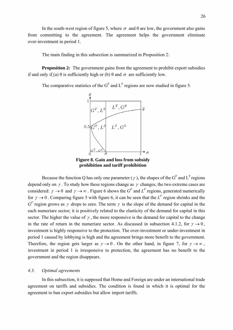
The comparative statistics of the GF and LF regions are now studied in figure 5.

Figure 8. Gain and loss from subsidy

prohibition and tariff prohibition

Because the function Q has only one parameter ( ), the shapes of the GF and LF regions

depend only on . To study how these regions change as changes, the two extreme cases are

considered: 0 and . Figure 6 shows the GF and LF regions, generated numerically

for 0 . Comparing figure 5 with figure 6, it can be seen that the LF region shrinks and the

GF region grows as drops to zero. The term is the slope of the demand for capital in the

each numeriare sector; it is positively related to the elasticity of the demand for capital in this

sector. The higher the value of , the more responsive is the demand for capital to the change

in the rate of return in the numeriare sector. As discussed in subsection 4.1.2, for 0 ,

investment is highly responsive to the protection. The over-investment or under-investment in

period 1 caused by lobbying is high and the agreement brings more benefit to the government.

Therefore, the region gets larger as 0 . On the other hand, in figure 7, for ,

investment in period 1 is irresponsive to protection, the agreement has no benefit to the

government and the region disappears.

4.3. Optimal agreements

In this subsection, it is supposed that Home and Foreign are under an international trade

agreement on tariffs and subsidies. The condition is found in which it is optimal for the

agreement to ban export subsidies but allow import tariffs.

27

Figure 8 combines figures 2 and 5. Consider the most interesting region of figure 8, i.e.,

the north-east region. In this region, the agreement that prohibits only export subsidies is

optimal compared to the following simple agreements: (a) the agreement that prohibits tariffs

and export subsidies; (b) the agreement that prohibits only tariffs; (c) the agreement that

prohibits only export subsidies; and (d) the agreement that prohibits nothing. The main result of

this paper can by summarized by Proposition 3.

Proposition 3: For sufficiently high σ and θ, the agreement that prohibits only export

subsidies is optimal among the simple agreements.

As mentioned above, whether the Home government gains or loses from an agreement

to prohibit tariffs depends only on its bargaining power (σ). With a sufficiently high bargaining

power, the Home government receives large political contributions from using tariffs and an

agreement to prohibit tariffs is not desirable. On the other hand, whether an agreement to

prohibit export subsidies is desirable to the Foreign government or not depends on σ and θ. For

a sufficiently high θ, the political contribution that the Foreign government receives from

export subsidies is highly eroded by free-riders and the government would be better off when

committing to prohibit export subsidies. Therefore, for sufficiently high σ and θ, the optimal

agreement is the one that prohibits only export subsidies.

5. Conclusion

This paper proposes a simple small-country model to explain the asymmetric treatment

between import tariffs and export subsidies in WTO. In the model, the anticipation of

protection creates inefficient investment. A government may choose to commit to a tariff

prohibition agreement and/or export subsidy prohibition agreement in order to eliminate this

anticipation and achieve a social welfare gain. However, when committing to these agreements,

that government loses the political contributions collected from protection. Therefore, that

government commits to a trade agreement, if the social welfare gain is greater than the loss in

political contributions.

In an environment where transportation costs are decreasing, export sectors grow and

import-competing sectors decline. In export sectors, export subsidies attract new entrants and

investment. These entrants erode the protection rent. The rent that the government can get from

protecting these sectors is, therefore, small. On the other hand, import-competing sectors

decline. In those sectors, the return on capital drops. Capital is sunk and cannot move out. This

sunk capital allows protection to raise the rate of return in these sectors without attracting entry

as long as the rate of return on the sunk capital is lower than the normal rate of return. The

protection rent in import-competing sectors is not eroded by new entrants and the government

may extract large political rent. In this environment, it is found that under the condition in

which the government has a high bargaining power and capital moves fast, the optimal

agreement prohibits only export subsidies and allows the use of tariffs.

28

References

Bagwell, K. and R. W. Staiger (2001). "Strategic trade, competitive industries and agricultural trade disputes, Economics and Politics, pp. 113-128.

——— (1999). "An economic theory of GATT," American Economic Review, vol. 89, pp. 215-248.

Baldwin, J. R. and W. Gu (2004). "Trade liberalization: Export-market participation, pro-ductivity growth and innovation", Oxford Review of Economic Policy, vol. 20, pp. 372-392.

Baldwin, R. and F. Robert-Nicoud (2002). "Entry and asymmetric lobbying: Why governments pick losers," NBER Working Paper No. 8756. National Bureau of Economic Research, Cambridge, MA, United States.

Bernard, A. B. and J. B. Jensen (2002). "The deaths of manufacturing plants," NBER Working Paper No. 9026. National Bureau of Economic Research, Cambridge, MA, United States.

Brander, J. A. and J. B. Spencer (1985). "Export subsidies and international market share rivalry," Journal of International Economics, vol. 18, No. 2, pp. 83-100.

Ethier, W. J. (2003). "Trade agreements based on political externalities", (mimeograph), University of Pennsylvania, United States.

Feenstra, R. C., J. Romalis and P. K. Schott (2002). "U.S. imports, exports and tariff data", NBER Working Paper No. 9387. National Bureau of Economic Research, Cambridge, MA, United States.

Glismann, H. and F. Weiss (1980). "On the political economy of protection in Germany", World Bank Staff Working Paper No. 427. . World Bank, Washington, D.C.

Grossman, G. and E. Helpman (1996). "Rent dissipation, free riding, and trade policy," European Economic Review, vol. 40, pp. 795-803.

——— (1995). "Trade wars and trade talks," Journal of Political Economy, vol. 103, No. 4, pp. 675-708.

——— (1994). "Protection for sale," American Economic Review, vol. 84, No. 4, pp. 833-850.

Hufbauer, G. and H. Rosen (1986). Trade Policy for Troubled Industries, Policy Analyses in International Economics 15, Institute for International Economics, Washington, D.C.

Hufbauer, G., D. Berliner and K. Elliot (1986). Trade Protection in the United States: 31 Case Studies, Institute for International Economics, Washington, D.C.

Johnson, H. (1954). "Optimum tariffs and retaliation," Review of Economic Studies, vol. 21, No. 2, pp. 142- 153.

Levy, I. P. (1999). "Lobbying and international cooperation in tariff setting", Journal of International Economics, vol. 47, pp. 345-370.

Maggi, G. and A. Rodriguez-Clare (2005a). "A political-economy theory of trade agreements", (mimeograph), Princeton University, United States.

———(2005b). "Import tariffs, export subsidies and the theory of trade agreements", (mimeograph), Princeton University, United States.

——— (1998). "The value of trade agreements in the presence of political pressures", Journal of Political Economy, vol. 106, pp. 574-601.

29

Mitra, D. (2002). "Endogenous political organization and the value of trade agreements", Journal of International Economics, vol. 57, pp. 473-485.

Rodrik, D. (1995). "Political economy of trade policy", in G. Grossman and K. Rogoff (eds.), Handbook of International Economics, pp. 1457-1495.

Staiger, R. W. and G. Tabellini (1987). "Discretionary trade policy and excessive protection", American Economic Review, vol. 77, pp. 823-837.

Subramanian, A. and S. J. Wei (2003). "The WTO promotes trade, strongly but unevenly", NBER Working Paper No. 10024. National Bureau of Economic Research, Cambridge, MA, United States.

Tornell, A. (1991). "Time inconsistency of protectionist programs", Quarterly Journal of Economics, vol. 106, pp. 963-974.

ARTNeT Secretariat

United Nations Economic and Social Commission for Asia and the Pacific

Trade and Investment Division United Nations Building

Rajadamnern Nok Avenue Bangkok 10200, Thailand

Tel.: +66 2 2882251 Fax.: +66 2 2881027

E-mail: artnetontrade@un.org Web site: http://www.artnetontrade.org

ARTNeT Working Paper Series are available from http://www.artnetontrade.org