Embed Size (px)
Citation preview
ASCEND IV
Advanced System for Computations in ENgineering Design
A portable mathematical modeling environment.Release 0.8
Sept 26, 1997Partial revision for release 0.9
June 20, 1998
Authors:Arthur Westerberg and research group
Department of Chemical Engineering, Carnegie Mellon UniversityBenjamin Allan, Vicente Rico-Ramirez, Mark Thomas, Kenneth Tyner
Other Helpful People Too Numerous To Mention Here
Sponsors 1993-1997:Computer Aided Process Design ConsortiumInstitute for Complex Engineered Systems
National Science Foundation grant for the Engineering Design Research CenterUS Department of Energy
We are deeply indebted to the authors and contributors at large who created Tcl/Tk. Many thanksDr. Osterhout!
Keywords:
ASCEND, CONOPT, EDRC, FORTRAN, GAMS, GNU license, GUI, ICES, LSODE, Leven-berg-Marquardt, MINLP, NLP, Newton, ODE, Tcl, Tk, UNIFAC, boundary value, chemical engi-neering, collocation, complex engineered system,, conditional modeling, copyleft, degrees offreedom, design, design research cente,r distillation, dynamic, engineering design, free software,freeware, initial value, initialization, interactive, large-scale, linear algebra, linear equations,mathematical modeling, mixed integer, modeling system, nonideal thermodynamics, nonlinearprogram, object oriented, optimization, ordinary differential equation, Pitzer vapor, reactive distil-lation, scalable, scaling, simulation, solving, structural analysis, Wilson liquid.

2
612244264
Documentation Bird’s Eye View
ASCEND IV 1Advanced System for Computations in ENgineering Design 1Documentation Bird’s Eye View 2Documentation Detail Map 4A typical scenario for running the ASCEND system 18Getting Started with ASCEND 22Script 26Library 38Browser 50Solver 60The Data Probe Window 72ASCPLOT 78Display slave 86ASCEND Units 90The ASCEND Toolbox 96The System Utilities Window 100Font Selection Dialog 108The Print Dialog 112Solved simple modeling problems with ASCEND 11A Conditional Modeling Example: Representing a SuperstructureA Simple Chemical Engineering Flowsheeting Example 1The ASCEND predefined collection of models 16The ASCEND IV language syntax and semantics 1Units library 218Brief History of ASCEND 232INDEX 236
/afs/cs.cmu.edu/project/edrc-ascend7/DOCS/Help/ascend-helpLOP.doc

3
Last modified: June 20, 1998 10:33 pm
4
8
ll
Documentation Detail Map
A typical scenario for running the ASCEND system 18Getting Started with ASCEND 22:: Philosophy 22- Getting the ASCEND system and installing it 22- Starting ASCEND 23
o ASCENDDIST 23o ASCENDHELP 23o ASCENDLIBRARY 23
Script 26Figure ASCEND’s Script Window 26
:: The Script Menu Bar 27- Script File Menu 27
o New File 27o Read File 27o Import File 27o Exit ASCEND 27o Save 27o Save As 27o Buffer List 27
- Script Edit Menu 27o Record actions 27o Select all 28o Delete statements 28o Cut 28o Copy 28o Paste 28
- Script Execute Menu 28o Run statements selected 28o Step through statements selected 2
- Script Options window 28o Save all options and appearances for a
windows 28- Script View window 29
o Font 29o Save Script appearance 29o Save all appearances 29
- Script Tools window 29- Script Help menu 29
o On SCRIPT 29o On getting started with ASCEND 29o About ASCEND IV 30
:: The Script Language 30- Summary 30
/afs/cs.cmu.edu/project/edrc-ascend7/DOCS/Help/ascend-helpTOC.doc
5
o <arg> 30o <a1,a2> 30o <a1 a2> 30o [a1] 30o [a,b] 30o qlfdid 30o qlfpid 30o {} 30
- Quick reference: 31o ASSIGN 31o BROWSE 31o CLEAR_VARS 31o COMPILE 31o DELETE 31o DISPLAY* 31o INTEGRATE 31o MERGE 31o PLOT 31o PRINT 31o PROBE 31o READ 31o REFINE 31o RESTORE* 31o RESUME 31o RUN 31o SAVE* 31o SHOW 31o SOLVE 31o WRITE 31
- Commands 32o ASSIGN 32o BROWSE 32o CLEAR_VARS 32o COMPILE 32o DELETE 32o DISPLAY 32o INTEGRATE 32o MERGE 33o OBJECTIVE 33o PLOT 33o PRINT 33o PROBE 33o READ 33o REFINE 34o RESTORE 34o RESUME 34
Last modified: June 20, 1998 10:33 pm

6
-
o RUN 34o SAVE 34o SHOW 34o SOLVE 34o WRITE 35o 35
:: Script Window Bindings 35o M1 35o M1-Drag 35o Shift-M1[-Drag] 35o Double-M1 35o Double-M1-Drag 35o Triple-M1 35o Triple-M1-Drag 35o M2 35o M2-Held-Down 35o M3 35o Control-M1 35o Control-k 36o Control-w 36o Meta-w 36o Control-y 36o Meta-y 36
Library 38Figure ASCEND Library Window. 38Figure Data structure used to store type defini
tions. 40:: Menu Bar 40- The file Menu 40
o Read types from file 40o Close window 41o Exit ASCEND 41
- The Edit Menu 41o Create simulation 41o Suggest methods 41o Delete Simulation 41o Delete all types 42Figure The Create Simulation Dialog 42
- The Display Menu 42o Code 42o Ancestry 42o Refinement hierarchy 42o External functions 42o Hide type 42o UnHide type 42o Hide/Show Fundamentals 43
/afs/cs.cmu.edu/project/edrc-ascend7/DOCS/Help/ascend-helpTOC.doc

7
7
Figure Select the fundamental type to Hide orUnhide. 43- The Find Menu 43
o ATOM by units 43o Type by name 43Figure The Library’s Find Type dialog. 44o Type by fuzzy name 44o Pending statements 44o To Display 44o To Console 44o To File 44
- The Options Menu 44o Generate C binary 45o Simplify compiled equations 45o Save options 45
- The View Menu 45o Font 45o Open automatically 45o Save appearance 45
- The export Menu 45o Simulation to Browser 46o Simulation to Solver 46o Simulation to Probe 46
- The help Menu 46o On LIBRARY 46
:: Type Refinement Hierarchy Window 46Figure The Type Refinement Window. 47Figure The Parts window displays the parts. 4Figure The Hierarchy Roots Window. 49
Browser 50Figure ASCEND’s Browser window. 50
:: The Menu Bar 51- BROWSER File menu 51
o Read values 51o Write values 51o Close window 51o Exit ASCEND 51
- BROWSER Edit Menu 51o Run method 51o Clear Vars 52o Set value 52o Refine 52o Merge 52o Compile 53o Resume Compilation 53o Create Part 53
Last modified: June 20, 1998 10:33 pm

8
9
- BROWSER Display menu 53o Attributes 53o Relations 53o Conditional Relations 53o Logical Relations 53o Conditional Logical Relations 54o Whens 54o Plot 54o Statistics 54
- BROWSER Find menu 54o By name 54o By type 54o Aliases 56o Where created 56o Clique 57o Eligible variables 57o Active Relations 57o Operands 57o Pendings 57
- BROWSER Options menu 57o Hide Passed Parts 57o Suppress Atoms 57o Display Atom Values 57o Check Dimensionality 58o Save Options 58o Hide Names 58o UnHide Names 58
- BROWSER view menu 58o Font 58o Open automatically 58o Save window appearance 58
- BROWSER Export menu 58o to Solver 58o Many to Probe 58Figure Filtering instances sent to the Probe 5o Item to Probe 59
- BROWSER Help menu 59o On BROWSER 59
Solver 60Figure Solver Window 60
:: The Solver Menu Bar 61- Solver File Menu 61
o Close Window 61o Exit ASCEND 61
- Solver Edit Menu 61o Remove instance 61
/afs/cs.cmu.edu/project/edrc-ascend7/DOCS/Help/ascend-helpTOC.doc

9
o Select objective 61- Solver Display Menu 61
o Status 61o Unattached variables 61o Unincluded relations 61o Incidence matrix 61Figure The Incidence Matrix 62
- Solver Execute Menu 62o Solve 62o Single step 62o Integrate 63
- Solver Analyze menu 63o Reanalyze 63o Debugger 63o Overspecified 63o Find dependent eqns. 63o Find unassigned eqns. 63o Evaluate unincluded eqns. 63o Find vars near bounds 63o Find vars far from nominal 64
- Solver View Menu 64o Font 64o Open automatically 64o Save Solver appearance 64
- Solver Export Menu 64o to Browser 64o to Probe 64
:: Solver Button Bar 64o Solver Select Button 64o Solver Options Button 65o Halt Button 65
- General parameters page 65Figure General Parameter Page 65
:: Available Solvers 67- QRSlv 67:: Debugger 69
Figure The Debugger Window 70The Data Probe Window 72:: Overview 72
Figure Probe window 73:: The File menu 73
o New buffer 73o Read file 74o Save 74o Save as 74o Print 74
Last modified: June 20, 1998 10:33 pm

10
o Close window 74o Exit ASCEND 74o Buffer list 74
:: The Edit Menu 74o Highlight all 74o Remove selected names 74o Remove all names 74o Remove UNCERTAIN names 74o Copy 74
:: The View Menu 75o Font 75o Open automatically 75o Save window appearance 75
:: The Export Menu 75o to Browser 75o to Display 75
:: The Probe Filter 75- The Help Menu 75
Figure Probe import filter 76ASCPLOT 78:: Plot maker 78
Figure The Ascend Plot Window 78- The Edit Menu 79- The Execute Menu 79
Figure The Create Data Window 80- The Display Menu 81
Figure The Graph Generics Window 82Figure Complete Plot 83
:: Navigation 84Figure Phase Diagram 85
Display slave 86:: Overview 86
Figure Display slave window 86:: Display File Menu 87
o Print 87o Close window 87o Exit ASCEND 87
:: Display Edit Menu 87o Cut 87o Copy 87o Paste 87
:: Display View Menu 87o Show comments in code 87o Save Display options 87o Font 87o Open automatically 88
/afs/cs.cmu.edu/project/edrc-ascend7/DOCS/Help/ascend-helpTOC.doc

11
-
o Save window appearance 88- Font 88- Open automatically 88- Display Help Menu 88:: Title line 88ASCEND Units 90:: The Menu Bar 90
o Units vs dimensions 90o Typical use 90Figure The Units of measure window 91
- Units File Menu 91o Read file 91o Save file 91o Close window 91o Exit ASCEND 92
- Units Edit Menu 92o Set precision 92o Set basic units 92
- Units Display Menu 92o Show all units 92
- Units View Menu 92o SI(MKS) set 92o US Engineering set 92o CGS set 92o Font 92o Open automatically 92o Save window appearance 92
- Units Help Menu 93:: An essay on units vs dimensions 93- On UNITS 94The ASCEND Toolbox 96
Figure The ASCEND Toolbox window. 96:: Exit 97:: Ascplot 97:: Help 97:: Utilities 97:: Internals 97:: Bug Report 98The System Utilities Window 100:: Overview 100
Figure The System Utilities window managesASCEND’s interaction with the operating system and with other programs. 100:: Variables 101- WWW Root URL 101- WWW Restart Command 102
Last modified: June 20, 1998 10:33 pm

12
4
- WWW Startup Command 102- ASCENDLIBRARY Path* 102
- Scratch Directory 103- Working Directory 103- Plot Program Type 103- Plot Program Name 103- Text Edit Command 103- Postscript Viewer 104- Spreadsheet Command 10- Text Print Command 104- PRINTER Variable* 104
- ASCENDDIST Directory* 104
- TCL_LIBRARY Environment Variable* 105
- TK_LIBRARY Environment Variable* 105
:: Buttons 105- OK 106- Save 106- Read 106- More 106- Help 106Font Selection Dialog 108:: Overview 108
Figure The font selection dialog. 108:: Font Menu 109:: Style Menu 109:: Cancel Button 109:: OK Button 109:: Current Font Sample 110:: Font Sampler Area 110:: Point Size Slider 110:: Current Font Selection 110:: Setting the Default Font 110The Print Dialog 112:: Overview 112
Figure The print dialog. 112:: Settings 112- Destination 112- Printer 114- Name of file 114- Enscript flags 114- User print command 114:: Buttons 115- OK 115- Help 115- Cancel 115Solved simple modeling problems with ASCEND 116
/afs/cs.cmu.edu/project/edrc-ascend7/DOCS/Help/ascend-helpTOC.doc

13
8
he
:: Roots of a polynomial 116- Problem statement 117- Answer 117:: Numerical integration of tabular data 11- Problem statement 118- Answer 119A Conditional Modeling Example: Representing a Superstructure122
Figure Superstructure used in the example of tapplication of the when statement122:: The WHEN Statement 122:: The Problem Description 124:: The Code 124A Simple Chemical Engineering Flowsheeting Example 144:: The problem description 144:: The code 145The ASCEND predefined collection of models 162
o system.a4l 162o atoms.a4l 162o Typical use of library files 163o Examples and scripts 163
The ASCEND IV language syntax and semantics 164:: Preliminaries 165- Punctuation 166
o keywords: 166o (* *) 167o ( ) 167o { } 167o [ ] 168o . 168o .. 168o : 168o :: 168o ; 168
- Basic Elements 168o L 169o M 169o T 169o E 169o Q 169o TMP 170o LUM 170o P 170o S 170o C 170
- Basic Concepts 175
Last modified: June 20, 1998 10:33 pm

14
:: Data Type Declarations 178o UNIVERSAL 179
- Models 179o MODEL 179o foo 179o bar 179o column(n,s) 180o flowsheet 180
- Sets 181o :== 181o UNION[setlist] 181o + 181o INTERSECTION[] 182o * 182o - 182o CARD[set] 182o CHOICE[set] 182o IN 182o SUCH_THAT (* 4 *) 183o | 183
- Constants 184o real_constant 184o integer_constant 184o symbol_constant 184o boolean_constant 184o :== 185
- Variables 185o ATOM 185o DEFAULT, DIMENSION, and DIMEN-
SIONLESS 185o real 186o integer 186o boolean 186o symbol 186o := 186o DATA (* 4+ *) 187o 188
- Relations 188o =, >=, <=, <, >, <> 189o MAXIMIZE, MINIMIZE 189o + 189o - 189o * 189o / 189o ^ 189o - 189
/afs/cs.cmu.edu/project/edrc-ascend7/DOCS/Help/ascend-helpTOC.doc

15
4
o ordered_function() 189o SUM[term set] 189o PROD[term set] 190o MAX[term set] 190o MIN[term set] 190
- Derivatives in relations (* 4+ *) 190- External relations 190- Conditional relations (* 4 *) 191- Logical relations (* 4 *) 191- NOTES (* 4 *) 191:: Declarative statements 194
o IS_A 195o IS_REFINED_TO 195o ALIASES (* 4 *) 195o ALIASES/IS_A (*4*) 195o WILL_BE (* 4 *) 195o ARE_THE_SAME 195o WILL_BE_THE_SAME (* 4 *) 196o WILL_NOT_BE_THE_SAME (* 4 *) 196o ARE_NOT_THE_SAME (* 4+ *) 196o ARE_ALIKE 196o FOR/CREATE 196o FOR/CHECK 196o SELECT/CASE (*4*) 196o CONDITIONAL (*4*) 196o WHEN/CASE (* 4 *) 196o IS_A 197o IS_REFINED_TO 197o ALIASES (* 4 *) 198o ALIASES/IS_A (*4*) 199o WILL_BE (* 4 *) 200o ARE_THE_SAME 200o WILL_BE_THE_SAME (* 4 *) 202o WILL_NOT_BE_THE_SAME (* 4 *) 202o ARE_NOT_THE_SAME (* 4+ *) 202o ARE_ALIKE 202o FOR/CREATE 203o SELECT/CASE (*4*) 204o CONDITIONAL (*4*) 204o WHEN/CASE (* 4 *) 204
:: Procedural statements 20o METHODS 204o ADD METHODS IN type_name; (*4*)
205o REPLACE METHODS IN type_name;
(*4*) 205
Last modified: June 20, 1998 10:33 pm

16
8
0
3
o ADD METHODS IN DEFINITIONMODEL; 205
o METHOD 205o FOR/DO statement 206o IF 207o SWITCH (* 4 *) 207o CALL 207o RUN 207
:: Parameterized models 20- The parameter list 208- The WHERE list 210- The assignment list 210- Refining parameterized types 21:: Miscellany 211- Variables for solvers 211
o solver_var 211o lower_bound 211o upper_bound 211o nominal 211o fixed 212o generic_real 212o solver_semi, solver_integer,
solver_binary 212o ivpsystem.a4l 212
- Supported attributes 213o (* 4+ *) 213
- Single operand real functions: 21o exp() 213o ln() 213o sin() 213o cos() 213o tan() 213o arcsin() 213o arccos() 213o arctan() 213o erf() 213o sinh() 213o cosh() 213o tanh() 214o arcsinh() 214o arccosh() 214o arctanh() 214o lnm() 214o abs() 214
- Logical functions 215o SATISFIED() (*4*) 215
/afs/cs.cmu.edu/project/edrc-ascend7/DOCS/Help/ascend-helpTOC.doc

17
18s li-
- UNITS definitions 215Units library 218:: Units 218:: The basic units in an extended SI MKS system 2:: Units defined in measures.a4l, the default system unitbrary of atoms.a4l. 219Brief History of ASCEND 232
Last modified: June 20, 1998 10:33 pm

18
d it
ingreeend
6, of
se
chit
ord
.ffel.
CHAPTER1 A TYPICAL SCENARIO FOR RUNNING
THE ASCENDSYSTEM
The ASCEND system is a modeling environment. We have designeto allow modelers to pose, debug and solve or optimize modelsdescribed by up to of the order of a hundred thousand nonlinearalgebraic equations on a conventional UNIX workstation or PC runnWindows NT4 or Windows 95. The ASCEND system comprises thmajor parts: the ASCEND modeling language for posing models, thASCEND interactive environment to allow users to compile, debug aexecute models, and a suite of solvers and optimizers.
Detailed information on modeling appears in Chapter 15, Chapter 1Chapter 17, and the Howto-ASCEND documents. The primary aimthis book is to describe the graphic user interface of ASCEND (amoving target if ever there was one) and to serve as a languagereference (Chapter 19). You would typically proceed as follows to uthe ASCEND GUI for modeling.
1. Using your favorite text editor (e.g., xemacs1), you will create amodel of the problem you wish to solve in the ASCENDmodeling language. ASCEND models are type definitions. Eamodel typically includes a declaration of the parts from which is constructed, including variables, instances of previouslydefined types and arrays of any of these. Each model alsoincludes the equations it adds to the model definition over andabove those equations that its parts will provide. Finally if youabide by our advice on model writing, you will also write three four methods that you will later run interactively on the compilemodel instance to prepare it to be solved.
If the model is particularly complex, you will probably createyour model using types defined earlier by yourself and othersFor chemical process flowsheet models, we provide a library otypes. We also provide a file that contains most of the types ovariables and constants anyone would use to construct a mod
2. Start up the interactive ASCEND user interface by typing
1. Xemacs is a very powerful text editor which is widely used on UNIX workstations. It is available for freefor both UNIX workstations and PCs through the WWW (search on xemacs).
/afs/cs.cmu.edu/project/edrc-ascend7/DOCS/Help/using_ascend.fm5
19 A TYPICAL SCENARIO FOR RUNNING THEASCENDSYSTEM
ch one
uy,otur
ss
lreou
l.
d alldel the
ed
ll-hemted
oon.
‘ascend’ on the Unix shell command line or double clicking onthe ASCEND icon on a PC. A number of different tool sets, earepresented by a special window, open up on the screen. Theyou will likely focus on at first is the SCRIPT window. In thiswindow under Tools, you will open whichever tool window youwant to work with at first, probably the LIBRARY tool set whichprovides tools to load text files containing ASCEND models.You will likely move and/or resize these windows.
3. Using a tool in the LIBRARY tool set, you will load the filescontaining the previously defined types of which your modelmakes use. You will open last the file containing the model yohave just written. Unless you are incredibly skilled and/or luckyou will see several error messages indicating that you have ncorrectly posed your model as the system attempts to load yonew file. Moving back to your favorite editor you will correctsyntax errors discovered by this file loading process, attemptagain to load, make more corrections, etc.
4. Once your new model description can pass the loading procewithout errors, you will compile a simulation for it. Again therecould be errors.
5. You will export this compiled simulation to the BROWSER tooset so you can look at the model, examining all its parts. If thewere compiler errors, you may use tools in this tool set to aid yto find exactly what you have done wrong in posing the mode
For example, if it is a particularly complex model, you willmethodically examine it to see if you have configured it as youwanted.
6. Once you are through inspecting the model and have removethe errors that of which you are aware, you will prepare the moto be solved. This you will do by asking the system to executemethods you should have written to go with your modeldescription. If you abide by the style of modeling that westrongly advocate, your model will have these methods attachto it -- written before your first atttempt to compile it. Thesemethods will be for setting initial values for the variables, forscaling the variables, and for setting the “fixed” flags for asufficient number of variables to make the model instance weposed. To be well-posed means a number of things, among tthat the model has the same number of variables to be calculaas equations available for calculating them.
7. You will next export the model to the SOLVER tool set. Whenimporting a model, the SOLVER tool set analyzes the model tdiscover how many variables and equations are in its descripti
Last modified: June 20, 1998 10:33 pm

20
itn
d
will
er
oth
itsle
illhat
h
o
,willel.g.ofpick
ldile
and
If it is not an optimization problem, the SOLVER looks to see ifis well-posed and, if not, will issue warning messages and opeup an interactive tool provided to aid you to make it well-poseright then and there. What you learn while using this tool youwill likely encode right away into the model description so thenext time you compile this model, it will become well-posedwithout this interactive step.
8. You can interactively choose among the available solvers and most likely choose our nonlinear equation solving solver. Withfingers crossed, you will ask the solver to start solving.
9. Whether or not it solves successfully, you will likely return to thBROWSER to inspect the results as you can view the value foevery variable and equation residual in the model using theBROWSER. If the solving process fails, you can select tools bin the BROWSER and the SOLVER to look for the likelyproblem. For example, you may have posed your problem andinitial conditions such that the solution is out of bounds. A toowill tell you if the SOLVER has driven any of the variables in thmodel to their bounds. Another will tell you if some of yourvariables are poorly scaled. Yet another will investigate themodel to see it if is locally singular, and if it is, that tool willreport to you exactly which equations (by name) have given itreason to believe that to be so. (In the near future, this tool walso tell you that you should change what you are fixing and wyou are calculating to remove this singularity, if such a movewould prove useful. It will give you a list of variables from whicto choose for each of these trades.)
10. You may wish to see the output in units different from thosecurrently used. Opening the UNITS tools set will allow you tochange wholesale from SI to American Engineering and/or tochange individual units such as those for pressure from bars tatm.
11. You may have opened the SCRIPT tool set before loading themodel files. Before doing all the above steps within ASCENDyou may then have activated a tool to record all the steps you subsequently take to load, compile, initialize and solve the modThis tool will construct a script from the steps it sees you takinYou wlil likely then edit this script, for example to delete some the missteps you have taken, and then save it. You may also out any of the steps in the script and execute them at any timerather than look for the tools in the tool set windows. You wouuse a script to aid you to repeat all the above steps quickly whyou are debugging a model. You will also prepare a script to hyour model to someone else to execute. Indeed, your first
/afs/cs.cmu.edu/project/edrc-ascend7/DOCS/Help/using_ascend.fm5

21 A TYPICAL SCENARIO FOR RUNNING THEASCENDSYSTEM
e
experience with ASCEND may be to run a script that someonelse has provided so you can be sure to run your first examplesuccessfully.Last modified: June 20, 1998 10:33 pm

A
ace
ry toave the
ions
ser,
n
E
with
CHAPTER2 GETTING STARTED WITH ASCEND
2.1 PHILOSOPHY
Our goal is to create a set of very powerful modeling/solving tools. side effect is that users can often find uses for the tools we did notanticipate. Another is that, while we have tried to build a user interfthat lets every user from beginner to expert use our tools (or theirscombined with ours!) in a comfortable fashion, we have almostcertainly erred on the side of giving the user too much control.Knowing that to be the case, the user should fearlessly dive in and tuse the system, at first by doing some of the simple problems we hprovided in this documentation. The first step, of course, is to startsystem up, the purpose of this section.
This chapter largely out of date. See howto-ascend.pdf and instructon http://www.cs.cmu.edu/~ascend/ascend_download.htm instead
2.1.1 GETTING THE ASCEND SYSTEM AND INSTALLING IT
ASCEND is available through our Web page. Using your web browgo the URL
http://www.cs.cmu.edu/~ascend/Home.html
Follow the instructions (the ftp link) there to download ASCEND.
Installing the UNIXversion
If you are downloading a version to run on a UNIX workstation, thefind someone who is a UNIX expert to help you. The process willinvolve transferring the source files for ASCEND along with a MAKfile. The MAKE file will allow a UNIX specialist to compile ASCENDand get it ready for use. There are detailed instructions that come
23 GETTING STARTED WITH ASCEND
s
ofto
ntt or
nt
.
not
sm
.
this version to help in installing it. (Your expert’s expertise may bevery minimally required for installing it on most systems.)
Installing the PCversion
If you are downloading to a PC running under either NT or Window95, you will be downloading ASCEND4.zip. Uncompress usingWinZip, double click on install.exe and follow the instructions.
2.1.2 STARTING ASCEND
2.1.2.1 FOR PC USERS ONLY
On the PC, simply double click on the ASCEND icon.
2.1.2.2 FOR UNIX USERS ONLY
The ASCEND IV interface is an open system written in TCL on top several libraries of C code. The users are expected to customize it suit their individual tastes.
We assume users are at least aware of the existence of environmevariables and X resources. If you are not, contact your UNIX experthe person who installed ASCEND on your system.
EnvironmentVariables
Normally, if you are running onUNIX your system administrator willhave set up a shell script to let you run ASCEND simply by typingascend . To see if this is true, try typingascend -hIf this doesn’t work, you may need to define the following environmevariables in your.login (or perhaps.profile ) file, or if you canfind the ASCEND binary, it will frequently run without requiring ashell script.
ASCENDDIST points to the directory where the ASCEND code has been installed
setenv ASCENDDIST /usr1/ballan/asc4/test
ASCENDHELP points to the ASCEND help file tree on your system. The tree doeshave to reside with the rest of the distribution, though it may. Thisshould have been configured for you when was installed.
ASCENDLIBRARY is a colon-separated list of directories where ASCEND looks for filewhich are required by other files or which are read into ASCEND froa script without giving a complete path name. If you do not defineASCENDLIBRARY, the system will make guesses that usually work
setenv ASCENDLIBRARY $ASCENDDIST/models/examples:$ASCENDDIST/models/libraries
Last modified: June 20, 1998 10:33 pm

PHILOSOPHY 24
/afs/cs.cmu.edu/project/edrc-ascend7/DOCS/Help/getting_started.fm5

25 GETTING STARTED WITH ASCEND
Last modified: June 20, 1998 10:33 pm

otherbed to
hich
CHAPTER3 SCRIPT
The Script Utility (see Figure 3-1) allows us to record the process of solving a model, or anyuser interface process. Once this process is recorded in the form of a script, the script can repeated either fully or in part. The solution process for a given model can be communicateanother modeler by distributing a script saved to a file. Following is an outline of the variousmenus and buttons on the script window along with a library of the ASCEND commands wcan be recorded.
Figure 3-1 ASCEND’s Script Window

27 SCRIPT
s
load
text
o
pthe
t ins,
the
s
ll you
e
3.1 THE SCRIPT MENU BAR
3.1.1 SCRIPT FILE MENU
The script file menu provides several functions for managing scriptfiles. The script utility may contain multiple scripts but will onlydisplay one at any given time. Upon startup a scratch workspace iprovided
New File Request a buffer name and creates a new buffer with this name.
Read File Requests a filename through the file selection box and proceeds tothis file (which is assumed to contain ASCEND Script and/or Tclstatements) into a new Script window buffer. No error checking isperformed on the loaded file.
Import File Requests a filename through the file selection box and appends thecontained in this file to the end of the current buffer.
Exit ASCEND Exit the ASCEND system. You will asked to confirm that you wish tdo this.
Save Saves the text in the current script buffer window to the current scrifile (indicated by the filename at the bottom of the script window). Texisting file is overwritten.
Save As Request a filename through the file selection box and saves the texthe current script buffer window to this file. If the specified file existit is overwritten.
Buffer List A list of scripts used in the current ASCEND session is displayed atbottom of the file menu. A script can be redisplayed in the scriptwindow by selecting it from the buffer list. This window contains thewords “License-Warranty.tcl” when you first start ASCEND (which ithe initial contents of the Script buffer).
Note: if you alter the contents (for example, clear it), the system wirestore the modified contents and not the original contents. The fileoriginally read remains unchanged unless you save to it.
3.1.2 SCRIPT EDIT MENU
Record actions When the record function is activated a log of interface events withdefined ASCEND Script commands is appended to the end of thecurrent script window buffer. Most, but not all, interface events hav
Last modified: June 20, 1998 10:32 pm

THE SCRIPTMENU BAR 28
d onrd
--se
sto
histo
r at
tedch
p to
he
ites
e
corresponding script commands. The record function can be turneand off by toggling the pull down button on the grill menu or the recobutton at the bottom of the script window.
Select all Selects (highlights) all text in the window. (A known bug exists hereif you do not place the cursor into the text buffer the first time you uthis tool, the highlighting may not occur although the text is in facthighlighted.)
Deletestatements
Removes (cuts) theselected text. The removed text is NOT saved forlater pasting.
Cut Cut highlighted text to the computer paste buffer. You can paste thitext into any application that supports cut, copy and paste -- e.g., inFramemaker or Excel.
Copy Copy highlighted text to the computer paste buffer. You can paste ttext into any application that supports cut, copy and paste -- e.g., inFramemaker or Excel.
Paste Paste the contents of the computer paste buffer into the Scipt buffethe point of the cursor.
3.1.3 SCRIPT EXECUTE MENU
Run statementsselected
This button takes the selected text, breaks it into statements delimiby any semicolons (;) that appear in the selection, and executes eastatement in the Tcl global environment.
Step throughstatementsselected
This button allows you to single step through the highlightedstatements. Two windows open: a small window that allows you toproceed to the next statement (next button), change from single sterunning the rest of the script automatically (go button) or stop (stopbutton) and the Display where, while single stepping, you will see tstatement being executed.
3.1.4 SCRIPT OPTIONS WINDOW
Save alloptions andappearances forall windows
This tool saves the complete current appearance of the ASCENDwindows and all the options selected anywhere in the system. It wrthe text fileascend.ad and a number of text files ending with.a4o intothe subdirectoryascdata in your “home” directory. The ascend.ad fileis a collection of the information placed into the .a4o files at the timyou run this instruction. Its main role is to aid in dubugging.
/afs/cs.cmu.edu/project/edrc-ascend7/DOCS/Help/script.fm5

29 SCRIPT
filexist
but is
can.
owefaultved
n
sely
u
tedonal
At any time, you can go into any of the windows and use theappropriate Save “window” appearance button to write a new .a4o for that window. You can also save new options where such tools ethroughout the system, resulting in other .a4o files. The newinformation in these .a4o files will not be reflected in ascend.ad file,it will be what is used to set window positions, etc., overriding whatin the ascend.ad file.
3.1.5 SCRIPT VIEW WINDOW
Font Opens the window that lets you reset the fonts for this window. You select the type of font, the style (bold, etc.) and the size for the font
Save Scriptappearance
Saves the current settings for this window for font settings and windsize and placement on your computer screen. These become the dsettings for opening this window in the future. These settings are sain a .a4o text file for this window which the sytem stores in thesubdirectoryascdata in your “home” directory.
Save allappearances
Saves a .a4o file for all the ASCEND windows. (See the aboveinstruction to see the purpose of these files.)
3.1.6 SCRIPT TOOLS WINDOW
Use the tools in this menu to open other windows in ASCEND whethey are closed or iconified.
This menu lists the major ASCEND windows. Selecting one of themwill open that window on your screen. See the help manuals for thewindows to find out more about them. This menu has almost exactthe same content as the ASCEND toolbox window. See thedocumentation corresponding to the toolbox for more details.
3.1.7 SCRIPT HELP MENU
On SCRIPT Brings up a text description of where to look for help on this window(i.e., it points to the pdf version of this document on the WWW.) Yomay, of course, look into the section mentioned in any local (butperhaps outdated) copy of the documentation.
On gettingstarted withASCEND
Brings up a text description of where to look for help on getting starwith using ASCEND -- the howto book (i.e., it points to the pdf versiof this document on the WWW.) You may, of course, look in any loc(but perhaps outdated) copy of the documentation.
Last modified: June 20, 1998 10:32 pm

THE SCRIPTLANGUAGE 30
w
ich
tlyy toill
About ASCEND IV Brings up a window telling you briefly about the GNU license andother information about the ASCEND IV software. This same windoopens the first time you start ASCEND on your computer.
3.2 THE SCRIPT LANGUAGE
3.2.1 SUMMARY
Script keywords are commands defined for ASCEND (in CAPS) whmay be used on the commandline or in the Script. Keywords areactually Tcl functions which encapsulate one or more of the Cprimitives and other Tcl procedures, so that the user can convenienemulate button presses. A working knowledge of tcl is not necessarbenefit from the Script’s functionality; however, the tcl literate user wbe able to create very powerful scripts.
Each keyword takes 0 or more arguments. The use of arguments isgiven in the following syntax:
<arg> indicates the use ofarg is required.
<a1,a2> indicates that the use of eithera1 or a2 is required
<a1 a2> indicates use of botha1 anda2 required. Usually written<a1> <a2>
[a1] indicates the use ofa1 is optional.
[a,b] indicates that eithera or b is optional, but not both.
qlfdid is short for ‘QuaLiFieD IDentifier’
qlfpid is short for ‘QuaLiFied Procedure IDentifier’
OF, WITH, TO, and other args in all CAPS are modifiers to thekeyword which make it do different things.
{} It is generally best toenclose all object names and units in {braces}to prevent Tcl from performing string substitution.
/afs/cs.cmu.edu/project/edrc-ascend7/DOCS/Help/script.fm5

31 SCRIPT
3.2.2 QUICK REFERENCE :
ASSIGN Sets the value of something atomic
BROWSE Exports an object to the browser
CLEAR_VARS Sets all the fixed flags to FALSE
COMPILE Compiles a simulation of a given type
DELETE Deletes a simulation or the type library
DISPLAY* Displays something
INTEGRATE Runs an IVP integrator
MERGE Performs an ARE_THE_SAME
PLOT Creates a plot file
PRINT Prints one of the printable windows
PROBE Exports an object to the probe
READ Reads in a model, script, or values file.
REFINE Performs an IS_REFINED_TO
RESTORE* Reads a simulation from disk.
RESUME Resumes compiling a simulation
RUN Runs a procedure
SAVE* Writes a simulation to disk
SHOW Calls a unix plot program on a file from PLOT
SOLVE Runs the solver
WRITE Writes values in Tcl format to disk
* Items not yet implemented.
Last modified: June 20, 1998 10:32 pm

THE SCRIPTLANGUAGE 32
the
id.
et
tial
3.2.3 COMMANDS
ASSIGN ASSIGN <qlfdid> <value> [units]
Sets the value of atom ‘qlfdid’ from the script. If value is real, it isrequired to give a set of units compatible with the dimensions of thevariable. If the variable has no dimensions yet, ASSIGN will fix thedimensions.
BROWSE BROWSE <qlfdid>
Exports qlfdid to the browser, displaying it as the current instance inbrowser.
CLEAR_VARS CLEAR_VARS <qlfdid>
Sets the value of the fixed flag to FALSE for all the variables on qlfd
COMPILE COMPILE <simname> [OF] <type>
Build a simulation of the type given with name simname. You can gaway with leaving out OF or spelling it wrong.
DELETE DELETE <TYPES,simname>
The modifier TYPES will cause all simulations to be deleted. If asimulation name (simname) is specified only that simulation will bedeleted.
DISPLAY DISPLAY <kind> [OF] <qlfdid>
How qlfdid is displayed varies with kind. kinds are: VALUEATTRIBUTES CODE ANCESTRY
INTEGRATE INTEGRATE {qlfdid args}
Runs an integrator on qlfdid. There are several permutations on thesyntax. It is best to have solved qlfdid before hand to have good inivalues.
INTEGRATE qlfdid (assumes LSODE and entire range)
INTEGRATE qlfdid WITH (assumes entire range)
INTEGRATE qlfdid FROM n1 TO n2 (assumes lsode)
INTEGRATE qlfdid FROM n1 TO n2 WITH integrator
/afs/cs.cmu.edu/project/edrc-ascend7/DOCS/Help/script.fm5

33 SCRIPT
Requires:
• n1 < n2
• qlfdid be of an integrable type (a refinement of ivp.)
MERGE MERGE <qlfdid1> [WITH] <qlfdid2>
ARE_THE_SAME qlfdid1 and qlfdid2 if possible.
OBJECTIVE OBJECTIVE
Semantics of OBJECTIVE that will be supported are unclear as noOBJECTIVE other than the declarative one is yet supported. Notimplemented yet
PLOT PLOT <qlfdid> [filename]
Writes plot data from qlfdid, which must be a plottable instance, tofilename.
PRINT PRINT <PROBE,DISPLAY>
Prints out the text currently in the Probe or Display.
PROBE PROBE ONE qlfdid
Exports the item qlfdid to the Probe.
PROBE ALL qlfdid
PROBE qlfdid
Exports items found in qlfdid matching the current specifications ofVisit in the Browser. By default, all variables and relations.
Items always go to currently selected probe context.
READ READ [FILE,<VALUES,SCRIPT>] <filename>
Loads a file from disk. Searches for files in directories (Workingdirectory):.:$ASCENDLIBRARY unless a full path name is given forfilename.
The modifier FILE is used to indicate that the file contains ASCENDsource code (ASCEND source code files normally have a .ascextension).
Last modified: June 20, 1998 10:32 pm

THE SCRIPTLANGUAGE 34
bles
be .s
)
T
the.
The modifier VALUES is used to indicate that the file contains variadata written by WRITE VALUES (These files normally have a .valueextension).
The modifier SCRIPT is used to indicate that the file is a script file toloaded at the end of the Script window (Script files normally have aextension).
If neither VALUES nor SCRIPT are found, FILE will be assumed.Note: You will get quite a spew from the parser if you leave out theSCRIPT or VALUES modifier by accident.
REFINE REFINE <qlfdid> [TO] <type>
Refines qlfdid to given type if they are conformable.
RESTORE RESTORE <file>
Reloads a simulation from disk
RESUME RESUME <simname>
Reinvokes compiler on simname.
RUN RUN <qlfpid>
Run the procedure qlfpid as if from the browser Initialize button.
SAVE SAVE <sim> [TO] <filename>
Filename will be assumed to be in Working directory (on utils pageunless it starts with a / or a ~. Not implemented yet.
SHOW SHOW <filename,LAST>
Invokes the plotter program on the filename given or on the file LASgenerated by PLOT.
SOLVE SOLVE <qlfdid> [WITH] [solvername]
Exports qlfdid to the solver and attempts to solve it with the defaultsolver (usually QRSlv) or the solver indicated by the optionalsolvername argument. Solvername must be given as it appears onmenu buttons. Bugs: Should use current solver rather than default
/afs/cs.cmu.edu/project/edrc-ascend7/DOCS/Help/script.fm5

35 SCRIPT
aS
.
thehe
a
me.
stelt
WRITE WRITE <kind> <qlfdid> <file> [args]
Write something (what sort of write indicated by kind) about qlfdid tofile. args may modify as determined by kind. At present only VALUEis supported. SYSTEM (for solver dump) would be nice.
WRITE VALUES filename.
Filename must be a full path name or in the pwd, also known as ‘.’
3.3 SCRIPT WINDOW BINDINGS
In the event binding descriptions that follow, M1 is short for mouse-button-1 (the left mousebutton), M2 is the middle button, and M3 is right mouse button. On machines with no middle button, M3 is still tright mouse-button and M2 is unavailable.
M1 repositions the cursor.
M1-Drag selects text.
Shift-M1[-Drag] extends the selection.
Double-M1 selects the nearest word.
Double-M1-Drag selects the nearest word and those you drag over, whole words at time.
Triple-M1 selects the nearest line.
Triple-M1-Drag selects the nearest line and those you drag over, whole lines at a ti
M2 does nothing.
M2-Held-Down has an effect similar to the scrollbar.
M3 does nothing.
Control-M1 Starts another part of a disjoint selection.
UNIX bindings: The text widgets in ASCEND share a common stack of cut/copy/patext pieces. This is a CMU extension of the text bindings, not defauTk behavior, and it is EMACS-like, but not EMACS (EMACS uses a
Last modified: June 20, 1998 10:32 pm

SCRIPTWINDOW BINDINGS 36
is is
onto
the
ftt
ring, not a stack.) When the stack is empty, Paste does nothing. Tha design decision. The Tcl function ascPopText can be changed tobehave differently.
Control-k Cuts text to the end of the current line, putting it on the stack.
Control-w Cuts the selected text, putting it on the stack.
Meta-w (e.g. diamond-w on most Sun keyboards) Copies the selected textthe stack.
Control-y Pastes the most recent text added to the stack, and removes it fromstack.
Meta-y Not supported.
MSW bindings: The standard Control-X, Control-C, Control-V bindings of MicrosoWindows clipboard apply to text widgets. The UNIX text stack is noavailable.
/afs/cs.cmu.edu/project/edrc-ascend7/DOCS/Help/script.fm5

37 SCRIPT
Last modified: June 20, 1998 10:32 pm

twoe
re
lla
CHAPTER4 LIBRARY
The Library window (Figure 4-1) in ASCEND allows the user to readtypes into the ASCENDsystem from files,compile types into instances, and delete types.
Types are the templates used to create simulations. They come in flavors: ATOM, which has a value associated with the instance namwhen it is instantiated, and MODEL, which has no value. ATOMs athe variables and constants in ASCEND; MODELs are the complexstructures one can build in ASCEND. ATOMs, further, come in vani
Figure 4-1 ASCEND Library Window.

39 LIBRARY
n,
,g
eft file
er
.f
and UNIVERSAL flavors. Universal atoms have a single compiledinstance which is global to all simulations created.
Both ATOMS and MODELS are defined in source files. By conventiosource files are named with the endings.a4c (ASCEND IV code)and .a4l (ASCEND IV library). You are free to use any other endingbut you will find the ASCEND file type filters you use when browsinfor files will be ineffectual.
In the ASCEND Library window, source files appears in the upper lbox. On the other hand, the types defined in the highlighted sourceappear in the upper right box. A double-button2 in either box willcompile the highlighted type definition. It doesn’t reselect. The uppleft box should perhaps have double-button2 bound to reread theselected source module. The ASCEND fundamental type such asinteger, real, etc., are not shown in the library window, since theirdefinition is performed internally, not by using a specific source fileThe lower box of the ASCEND Library window contains the name othe simulations that have been compiled and can be run.
The data structure used to store type definitions is sketched inFigure 4-2.
Last modified: June 20, 1998 10:32 pm

MENU BAR 40
is
of a
me, a
4.1 MENU BAR
The menu bar on the Library window has eight entries: File, Edit,Display, Find, Options, View, Export and Help.
4.1.1 THE FILE MENU
Read types fromfile
This loads type definitions into the system. The file selection dialogused to select a source file.
The names of types are unique within the system. A new definition type overwrites the old definition of a type in all cases. If the newdefinition and the old definition were read from files of the same nathis overwrite will be done silently. If the new definition comes from
Type Library
type desc 1
type desc 2 type desc 3
Notes: type desc3 has a refinement ptr to type desc 2 type desc2 has a refinement ptr to type desc 1
The problem is when type desc 2 is being redefined by reloading a new module.
Figure 4-2 Data structure used to store type definitions.
/afs/cs.cmu.edu/project/edrc-ascend7/DOCS/Help/library.fm5

41 LIBRARY
w
ry
piesaryee,pe.
h
imen
of
tedthedrite
the
hetee
different file, the overwrite will be done noisily.
This is incorrect, but perhaps is as it ought to be.Existing typeswhich refined or had parts that were of the old type definition will norefine or have parts which are of the new type. e.g. If you rereadsystem.asc (and hence solver_var) everybody in the interface librawho pointed at the old solver_var type will now point at the newsolver_var type.
Instances already compiled using the definitions that have beenoverwritten will continue to point at a copy of the old definition thesystem has squirreled away somewhere. These squirreled away cowill not necessarily be the same as what is in the interface type librif you have reread a file with a newer type definition. This may causrefinement of the old instance to fail. In general if you redefine a typyou will probably want to reinstantiate things that depend on that ty
Close window It closes the ASCEND’s Library window. To reopen, use the Toolsmenu in the Script window or use the SCRIPT tool in the Toolbarwindow.
Exit ASCEND Exit the ASCEND system. You will be asked to confirm that you wisto do this.
4.1.2 THE EDIT MENU
Createsimulation
Create (or instantiate) a simulation based on a type definition. Anytthat the compile button is selected, the compile dialog window showin Figure 4-3 will ask for the name which will be used to identify thesimulation. All simulation created can be seen and in the lower boxthe ASCEND Library window. This box can contain any number ofsimulations.
Suggest methods Pick any type in the right window and apply this tool to write suggesmethods for that type. See the Howto book, Chapter 2, for a list of methods we suggest one should write for models. These suggestemethods are prototypes which you can cut and paste into your favotext editor. You should be carefully edit them before adding them tomodel type definition.
DeleteSimulation
This tool works to remove previously compiled simulations listed in tbottom subwindow of the Library window. Select a simulation to deleand use this tool to eliminate it from ASCEND. ASCEND will clear thmodel from the Browser and Solver. Items placed into the Probewindow are not deleted.
Last modified: June 20, 1998 10:32 pm

MENU BAR 42
ffectr
e the
lay
ND
be all
lt”.
u.
Delete alltypes
Destroys all simulations and deletes all types. This option has no ein the fundamental definitions. Deleting all types clears the Browseand Solver windows, but not the Probe window.
4.1.3 THE DISPLAY MENU
Most of the options in the Display Menu will be enabled only if a typdefinition has been selected; this is because the tasks performed inmenu are implicitly associated with a type definition.
Code Displays the source code of the selected type in the ASCEND DispWindow.
Ancestry Allows the use of the Type Refinement Hierarchy Window. SeeSection 4.2 on page 46 documenting this window.
Refinementhierarchy
Displays the refinement hierarchy of the selected type in the ASCEDisplay window.
Externalfunctions
Display in the Display window any external function defined from aloaded package library.
Hide type The Browser will not display any type definition which you select to hidden with this tool. You may select to hide the type or the type andits refinements. For example, doing the latter withsolver_var willhide all variables in a compiled instance of the model.
UnHide type Reverses the action of “hiding” a type. Select the type in the rightwindow and select unhide if that tool is lit. The Browser willimmediately begin to display this previously hidden type. The defaufor all the type definitions (except fundamentals) is to be “unhidden
Both Hide Type and UnHide Type have two selections as a submenThe user can ask for the un/hiding of only theselected type, or for theun/hiding of the selectedtype and its refinements.
Figure 4-3 The Create Simulation Dialog
/afs/cs.cmu.edu/project/edrc-ascend7/DOCS/Help/library.fm5

43 LIBRARY
ar asbleeing
ary
ctou
Hide/ShowFundamentals
This special option is given because fundamental types do not appedefinitions in the ascend libraries, but we still may want to able/enasuch types for browsing purposes. When this button is selected, thwindow shown in Figure 4-4 will be used to perform the desired hidor unhiding of any of the fundamental types.
4.1.4 THE FIND MENU
ATOM by units This extremely handy tool allows you to find all the ATOMS that arecurrently loaded into the library whose dimensionality conforms to auser specified set of units. For example, if you have loaded the libratoms.a4l into the Library, then you can use this tool to find all atomdefinitions that could be expressed in ft^3 or in kJ/mol. To use, selethe tool. In the window that opens type in the units and select OK. Ydo have to know the units ASCEND will recognize. Open the Unitswindow and under the Display menu select Show all units for acomplete list.
Type by name Finds a type by its name. The type will become the current typehighlighted in the Library right and left upper windows.
Figure 4-4 Select the fundamental type to Hide or Unhide.
Last modified: June 20, 1998 10:32 pm

MENU BAR 44
tchme
,
ns
es
on
w
el
se.f
beect.
Type by fuzzyname
Finds all type names currently loaded in the Library window that maa word (provided by the user) in any fuzzy way. For instance, the nacolumn would list the following: demo_column, mw_demo_column,plot_column, etc. if these were currently loaded in the Library. Thefuzzy name is defined in a dialog window similar to that used in theFind Type by name option.
Pendingstatements
There are three selections under the Pending Statements submenuthese areTo Display, To Console, andTo File. Pendings in asimulation are relations that have not yet been fully processed byASCEND’s compiler. It is the modeler’s job to correct the pendingrelations in order to arrive at a fully functional simulation. Correctiomay be made by either creating a model which refines the currentmodel or by editing ASCEND code and starting over. This option givthe user access to information about the type and location of thepending statements. Often pending statements arise from a commcause such as a incorrectly qualiified or misspelled name for a set.
To Display By selecting theTo Display option, all of the simulation pendings aredisplayed in theDisplay window.
To Console By selecting theTo Console option, all of the simulation pendings aredisplayed in the Console window (in UNIX, the Console is the windofrom which you started ASCEND IV).
To File By selecting theTo File option, theFile select box is opened and theuser is asked to enter the name of the file in which to save the modpendings.
4.1.5 THE OPTIONS MENU
The titles for most of these tools more or less describes their purpoWe will not describe them With these options, you can turn on or ofmessages ASCEND will generate while compiling. Turning offwarning and error messages will, of course, mean that you will not told about problems your model may have that we were able to det
Figure 4-5 The Library’s Find Type dialog.
/afs/cs.cmu.edu/project/edrc-ascend7/DOCS/Help/library.fm5
45 LIBRARY
ch be
non isetion
s
his
can.
owefaultved
Since ASCEND will still compile in spite of warning messages (whigenerally reflect your model does not conform to what we believe togood modeling practice), you may wish to suppress them. See theHowto Book, Chapter 2 for a discussion of good modeling practice.
We describe only those tools that do not turn on and off compilermessages.
Generate Cbinary
If you have a C compiler installed and ASCEND knows about it, theyou may elect to have ASCEND compile C code to evaluate equatiresiduals in ASCEND. The compiler finds and will, when this optionselected and possible, compile only a piece of code for each uniquequation type, of which there are very few in any model. The evaluaof residuals will be much faster using compiled C code.
Simplifycompiledequations
This option is on by default. ASCEND will reduce terms in equationsuch as a product of constants whose values it knows to a singleresultant constant when you select this option. Whole terms inequations may disappear if ASCEND finds them multiplied by theconstant zero.
Save options Save the current setting for all the options selected using items in tmenu. ASCEND put the saved information into a text filelibrary_opt.a4o and which it then saves in theascdata subdirectory ofyour “home” directory.
4.1.6 THE VIEW MENU
Font Opens the window that lets you reset the fonts for this window. You select the type of font, the style (bold, etc.) and the size for the font
Openautomatically
Toggles a switch which, if set, will cause this window to openwhenever anything is placed into it.
Save appearance Saves the current settings for this window for font settings and windsize and placement on your computer screen. These become the dsettings for opening this window in the future. These settings are sain a .a4o text file for this window which the sytem stores in thesubdirectoryascdata in your “home” directory.
4.1.7 THE EXPORT MENU
There are three selections under this submenu, these areSimulation toBrowser, Simulation to Solver, andSimulation to Probe.
Last modified: June 20, 1998 10:32 pm

TYPE REFINEMENT HIERARCHY WINDOW 46
l.
om
me.ir
u
ert
the
ion.
Simulation toBrowser
By selecting theSimulation to Browser option, the simulationhighlighted in the lower box of the Library window is loaded into theBrowser. From theBrowser, the model can be explored in more detai
Simulation toSolver
By selecting theSimulation to Solver option, the simulationhighlighted in the lower box of the Library window is loaded into theSolver. (Note that exporting to the solver causes a degrees of freedanalysis to be carried out.)
Simulation toProbe
By selecting theSimulation to Probe option, all of the variables of thesimulation highlighted in the lower box of the Library window areloaded into theProbe. This is not recommended as there are usuallymore variables in a model than the user would wish to view at one tiHowever, if the user does wish to look at all of the variables and thecurrent values, theSimulation to Probe option can be useful.
4.1.8 THE HELP MENU
On LIBRARY Brings up a text description of where to look for help on this window(i.e., it points to the pdf version of this document on the WWW.) Yomay, of course, look into the section mentioned in any local (butperhaps outdated) copy of the documentation.
4.2 TYPE REFINEMENT HIERARCHY WINDOW
The type tree is a directed acyclic graph (DAG) based on the typehierarchy currently defined in the interface Library. Selection of thetool Display Ancestry (mentioned above when describing tools undthe Display menu) for any selected type gives the entire refinemenhierarchy for that type, by enabling the use of the window shown inFigure 4-6.
The current focus in the hierarchy is indicated by a rectangle aroundtype name and the Current type.
The buttons on the left in the type window operate on the currentlyselected type:
‘Atoms’ shows the types of ATOMic parts in the selected typedefinition. It also shows the incremental code for the type. You canselect from the part types list to look at a different hierarchy.
‘Code’ shows the internally stored code of the selected type. Theexpressions, both algebraic and logical, are in reverse Polish notat
/afs/cs.cmu.edu/project/edrc-ascend7/DOCS/Help/library.fm5

47 LIBRARY
d
This is different from the way the code of the Library Display Codebutton shows it. Comparison of the two is sometimes a usefuldebugging tool.
‘Parts’ (Figure 4-7)shows the types of MODEL parts in the selected
type definition. It also shows the incremental code for the type.
The ‘<<<‘ (or backtrack) button backs up to the previously displayetype hierarchy, if there is one.
Figure 4-6 The Type Refinement Window.
Figure 4-7The Parts window displays the parts.
Last modified: June 20, 1998 10:32 pm

TYPE REFINEMENT HIERARCHY WINDOW 48
ing
hisr
rt
ame stillnll
‘Roots’ (Figure 4-8) shows the existing root types, that is, the existtypes which are not refinements of anything.
While ASCEND is building the graph, you may see a spew in thewindow from which ASCEND was started about orphaned types. Tmeans there are types in the Library which are refinements of oldetypes which are no longer in the Library.
While ASCEND is getting the Atom or Model parts list for a type, patypes names which are undefined will be spewed.
When an older type is replaced in the Library by a new one of the sname, the old one is squirreled away where types that refined it cansee it. The only way to get current types to look at the new definitiowithout touching the source files for the current types is to delete atypes and reread the entire Library.
/afs/cs.cmu.edu/project/edrc-ascend7/DOCS/Help/library.fm5

49 LIBRARY
Figure 4-8 The Hierarchy Roots Window.
Last modified: June 20, 1998 10:32 pm

ars inightstackin thisnd it’s any
CHAPTER5 BROWSER
The Browser window (Figure 5-1) provides the means with which to view the parts of asimulation. When a simulation is exported to the Browser, the name of the simulation appethe Browser’s upper left box and the child instances of the simulation appear in the upper rbox. Selecting a child instance in the right box will move the instance to the bottom of the in the left box and display it’s children in the right box. The instance tree can be traversed manner until an atom (usually a variable) resides at the bottom of the stack in the left box aattributes appear in the right box. Selecting a member of the stack in the left box will clearlower instances on the stack and display the selected instance’s children in the right box.
Figure 5-1 ASCEND’s Browser window.

51 BROWSER
stances
e
showne
lowernce inutton
n in
ues).ly thean
areed
dR
h
dit -
A subset of the instances appearing in the upper right box as well as the values of these inappear in the Browser’s lower box. Which subset of instances appears in the lower box iscontrolled by the user by clicking in some of the options given in the bar at the bottom of thBrowser window. In Figure 5-1 RV has been selected. RV stands forRealVariables. Therefore,the child instances of fl1 which are real variables and the values of these real instances arein the lower box. Other options in the bar at the bottom of the Browser window, which can bsimultaneously selected, are DV (Discrete Variable), RR (Real Relations), LR (LogicalRelations), RC (Real Constants) and DC (Discrete Constants). Selecting an instance in thebox with the right button of the mouse will have the same effect as selecting the same instathe upper right box. On the other hand, selecting an instance in the lower box with the left bof the mouse will bring up the “Set Value” Dialog box, which will give the user the option ofmodifying the value of the selected instance. More about the “Set Value” option will be givethe following section of this document.
5.1 THE MENU BAR
• The menu bar on the Browser window has eight entries: File,Edit, Display, Find, Options, View, Export, and Help.
5.1.1 BROWSER FILE MENU
Read values Reads the values from a file previously saved by Write Values. Valfiles are read using full path names (including the simulation nameThe simulation for which values are being read does not necessarihave to be in the Browser (but it should exist). You may specify thatvalues are to be read into a different simulation or simulation part ththey were originally saved from, provided the old and new locationscompatible. If the original simulation does not exist, you will be askfor a new simulation name.
Write values Saves the values for the instance in the Browser to a file for laterrereading.
Close window Closes the Browser window. To reopen, go to the Script window anselectInstance browser under the tools menu or select the BROWSEon the Toolbox window.
Exit ASCEND Exit the ASCEND system entirely. You will be asked if you really wisto complete this instruction.
5.1.2 BROWSER EDIT MENU
Run method If the instance in the left box has one or more methods available, E>Run Method will be available for selection. Selecting Run Method
Last modified: June 20, 1998 10:32 pm

THE MENU BAR 52
a
tion
e). a
eteheened
t
box.athifies
may of thent type forment
ithou
will display the Methods Selection Window containing a list ofavailable methods for the current Browser instance. A method isselected by clicking it’s name (only one method can be selected at time). Depressing the OK button will run the selected method.Depressing the Show button will display the code for the selectedmethod. Depressing the Cancel button will close the Method SelecWindow without running any method.
Clear Vars In ASCEND, the type solver_var and all its refinements constitute avariable for solution purposes. Each variable has a boolean, named“fixed”, as one of its children. When a variable’s fixed boolean, orfixed flag as it is commonly called, is set to False, the variable isconsidered an output variable (i.e. the solver will determine its valuThe Clear Vars method sets the fixed flag of every variable which ischild of the current Browser instance to False.
Set value When the current Browser instance is a real, symbol, integer, orboolean Edit->Set Value will be available for selection. Selecting SValue displays the Set Value Dialog box. The value (and units in thcase of reals) may be set by filing in the value (and units) fields of tSet Value Dialog box and depressing the OK button. Depressing thCancel button closes the Set Value Dialog box. Booleans are assigsimply by double clicking the mouse button 2 on their name when iappears in the right browser box.Write values
Selecting Edit->Write Values saves the attribute values of all atomswhich are descendents of the current instance to a file. A file selectis displayed so a new file may be created or an old file over writtenThe attribute values are written to the selected file along with their pnames relative to the current instance. The first line of the file specthe path from the simulation to the current instance.
Refine Refines the current Browser instance to a given type. Edit->Refine only be selected if the Library contains types which are refinementsthe current Browser instance type. Selecting Edit->Refine displayseligible types for the refinement of the current part in the Refinemedialog box. Selecting a type and depressing OK refines the currentto the selected type. Depressing Show displays the ASCEND codethe selected type. Depressing the Cancel button closes the Refinedialog box without making any refinements.
Merge ARE_THE_SAME the current part (left side of the Browser) withanother given part. Do not ARE_THE_SAME parts from 2 differentsimulations. You cannot merge parts of atoms (which are atomic) wanything. The dialog box will ask for the name of the instance that y
/afs/cs.cmu.edu/project/edrc-ascend7/DOCS/Help/browser.fm5

53 BROWSER
eed
d a aew
.nne.
r isch
l in
ione
the
t of
al
want to merge with the instance highlighted in the left box of thebrowser.
Compile Submenu containing Resume Compilation and Create Part.
ResumeCompilation
Attempts to process any pending statements in the simulation in thBrowser. It does not matter where in the simulation you have browsto, Resume always starts at the top.
Create Part This is a feature of the PASCAL version only. The proper way to adpart to a simulation is to create a refinement of the original model innew file, read in that definition, and refine the simulation up to that nmodel.
5.1.3 BROWSER DISPLAY MENU
Attributes Display the attributes of a real variable. Other functionality may beadded later to this button.
Relations Display all the relations at or below the current point in the BrowserRelations get arbitrary names unless explicitly named by the user icode. The arbitrary name, at the moment consists of ParentName_where n is the number of the nth relation in the MODEL ParentNamIf this name is not unique, enough letters a-z get added to make itunique. When the instance highlighted in the left box of the Browsea real variable, this option will display all of the relation in which sua variable is incident.
ConditionalRelations
Display all the conditional relations in or in the children orgrandchildren etc., of the current object in the Browser. ConditionaRelations do not have to be satisfied. They are used as boundariesconditional programming. The arbitrary name of a conditional relatis obtained in the same way as any other relation, but in general, thname of a conditional relation must be provided by the user, since operator SATISFIED requires such a name.
LogicalRelations
Display all the logical relations in or in the children or grandchildrenetc., of the current object in the Browser. Logical Relations getarbitrary names unless explicitly named by the user in code. Thearbitrary name of a Logical Relation follows the same pattern as thareal relations. When the instance highlighted in the left box of theBrowser is a boolean variable, this option will display all of the logicrelation in which such a boolean variable is incident.
Last modified: June 20, 1998 10:32 pm
THE MENU BAR 54
ns
lut in by
will
one.laysr in
nd
eyles
hetion cannd box
tes.
rch
ConditionalLogicalRelations
Display all the logical relations in or in the children or grandchildrenetc., of the current object in the Browser. Conditional Logical Relatiodo not have to be satisfied. They are used as conditions to check inconditional programming.The arbitrary name of a conditional logicarelation is obtained in the same way as any other logical relation, bgeneral, the name of a conditional logical relation must be providedthe user, since the operator SATISFIED requires such a name.
Whens This option is enabled for instances of models, relations, booleans,symbols, and integers. For the case of a model instance, this buttondisplay not only all the when instances defined as parts of such amodel, but also the when instances which include such a model in of their CASEs. Distinction is made between those two possibilitiesFor relation, boolean, symbol and integer instances, this option dispthe when instances which include such relation, symbol, etc., eitheone of their CASEs or in the list of conditional variables. Wheninstances are useful for the conditional configuration of a problem aalways get arbitrary names.
Plot Invokes a plotting program, if allowable, on the current object. Thetype of plot generated is controlled by the Utilities page variablesPlot.type and Plot.program. See the relevant chapters in the Howtomanual on plotting to find the types which ASCEND will plot. Also sethe ASCEND library of models supporting plotting: plot.a4l (and anof the other model files containing the name plot which have exampof plotting within them).
Statistics Prints out some information about the object tree in the Browserstarting with the current object and going downward through itschildren, grandchildren, etc.
5.1.4 BROWSER FIND MENU
By name Search for an instance with a given qualified name and go there. Tname of the instance to search for is defined in the dialog. This opmay be useful for jumping around in the instance tree. Since namesbe quite long, you may find this tool most useful when you have fouthe name elsewhere and can cut and then paste it into the dialoguethat opens for this tool.
By type You can search for objects of any particular type with certain attribuThe default type will list all fixed solver_vars for the problem. Theallowable searches are best explained by examples as shown inTable 5-1 (with the third being the default just mentioned). The sea
/afs/cs.cmu.edu/project/edrc-ascend7/DOCS/Help/browser.fm5

55 BROWSER
s,
oreemgt of
erese.
is loosely matched, i.e. any object that is of the type given, OR arefinement of the type given and matches the attribute qualificationwill be on the list of items found.
If there are no matches, there is no results box: just a message in apopup error message.
The results of the Find appear in a box and you can export one or mof the results in the box to the Browser or the Probe by selecting thand clicking on Browser or Probe. When you have finished exportinitems to wherever you like, click on OK. Do close this box as the resthe interface will ignore you until you do.
Notes:
• Clear any of the extra fields not required for your search beforyou hit OK. We will usually find nothing that matches if there aextra search parameters hanging around that don’t make sen
Table 5-1 Examples of the performance of the Find by type option
Type Attribute Low Value High Value Explanation
unit Find all parts that are units.solver_var fixed Find all refinements of solver_var
with a part fixedsolver_var fixed TRUE Find all refinements of solver_var
with a part fixed wherefixed==TRUE
stream Ftot 4 Find all streams with part Ftotwhere value is 4+ epsilon
stream Ftot 4 10 Find all streams with part Ftotwhere 4 <= Ftot <= 10
relation VALUE 0 Find all relations with a residual0 + epsilon
symbol VALUE ACH Find all symbols where VALUE is‘ACH’
symbol VALUE ACH ACZ find all symbols where ‘ACH’ <=VALUE <= ‘ACZ’
component_constant Find all parts that arecomponent_constants
symbol_constant VALUE UNDEFINED Find all undefinedsymbol_constants. Works for alltypes with a value.
Last modified: June 20, 1998 10:32 pm

THE MENU BAR 56
an
ueisine
hat
ts in
ght
f). by
tity.
n.umee twot
the
ans
• VALUE is a special keyword for dealing with atomic types.Variables and symbols have a value internally but not a childnamed VALUE. Similarly, relations have a residual but not as accessible part with that name.
• Symbols and integers will be matched exactly if only a low valis given. The matching of symbols given a low and high value done lexically according to the collating sequence of the machin use.
• Frequently what you really want to see is the name of a set ofthings of a given type -- e.g. a case where you want to know wcomponents are in a flowsheet. Find will return the instancesthough, not their common parent. Simply export one to theBrowser and then click up a level to see the set of componenuse.
• You can tab between fields in the Find by Type widget.
• You can select a type name in the library. Pick the type in the riwindow. Its name will appear in the lower middle window.Highling the name and use the typical method to copy a set ohighlighted characters for your computer (e.g., Ctrl-c on a PCThen use the typical way to paste into the type slot of the FindType Window (Ctrl-v on a PC).
• Epsilon is about 1e-8 in terms of the SI units for any real quan
Aliases Find all the other names that the current object has in the simulatioFor example, assume that you have named a simulation as fs. Assfurther that the output stream from the mixer, m1, is merged with thinput stream for the reactor, r1. Then, that stream is an object withdifferent names. Suppose you are looking at r1.feed as the currenobject. Asking for aliases will give the list
fs.r1.feed
fs.m1.output
If you pick one of the aliases, it can be exported to the BROWSER,SOLVER or the PROBE. Alternate names for objects can also becreated by ALIASES statements and by passing them into aparameterized MODEL.
Where created Find the other names that the current object was CONSTRUCTEDunder. If an object is shown as being created under 4 names, it methat once there were 4 objects and that 3 were destroyed in merge
/afs/cs.cmu.edu/project/edrc-ascend7/DOCS/Help/browser.fm5

57 BROWSER
is
the
f
e issl
k
heeese
l orso
orehe
to
jectd by a
s ofe ofby.
(ARE_THE_SAME) statements to reach the current unity. (Mergingexpensive).
If you pick one of the names, it can be exported to the BROWSER,SOLVER or the PROBE. Alternate names for objects can also becreated by ALIASES statements or by passing them into aparameterized MODEL, but these names do not appear in the list ocreations.
Clique Find all the instances that ARE_ALIKE with the current one. Theinstances shown are bound together so that if the formal type of onchanged, they are all upgraded with the first. Parameterized objectcannot be ARE_ALIKE’d because when parameters exist the formatype requires outside information (the parameters) in order to checthat it is being used in a valid way.
Eligiblevariables
Find real variables eligible to be fixed. If the solver is occupied by tsame simulation, this query is thrown to the Solver. If not, the degrof freedom are analyzed as if the current model were exported to thSolver.
ActiveRelations
Find all the relations of the current object. You may tag one, severaall of the relations found and export them to the Probe. You may alexport the first tagged relation to the Browser.
Operands If the current object is a relation, list all the operands in it. One or mof these may then be exported to the Probe. You may also export tfirst tagged operand to the Browser.
Pendings List in the Console window all the statements that the compiler failedcompile for the current Browser object.
5.1.5 BROWSER OPTIONS MENU
Hide PassedParts
Toggles the display of parts which were passed into the Browser obas passed parameters. Note that these shared objects were createparent (or grandparent, etc.) of the current Browser object and willappear on the list of parts for that parent.
Suppress Atoms This button toggles whether or not to show atomic instances in theupper right box of the Browser window.
Display AtomValues
This button toggles whether to display values or to display the typeatoms in the child box (upper right side) of the Browser. For the casrelations, the residual shown with the relation is the last computed the solver and not the residual at the current values of the variables
Last modified: June 20, 1998 10:32 pm

THE MENU BAR 58
Inel it
the
ors byith
can.
en
owefaultved
t
or
CheckDimensionality
This switch turns warnings about relation inconsistency off and on.principle it should not be necessary, but for the quick and dirty modis sometimes handy.
Save Options Save the current options in this menu. When you restart ASCEND,system will reset the options to these saved settings.
Hide Names This option has a similar functionality from that of Hide Types in theASCEND Library windows. That is, it will hide or unhide instances fbrowsing purposes. The difference, however, is that this option hidename, not by type. To clarify, it is quite different to hide instances wthe name fs than to hide all instances of type test_flowsheet.
UnHide Names Reverses the effect of the command Hide Names. A list of hiddennames appear from which you can select what to unhide..
5.1.6 BROWSERVIEW MENU
Font Opens the window that lets you reset the fonts for this window. You select the type of font, the style (bold, etc.) and the size for the font
Openautomatically
Toggles a switch which, if set, will cause the Browser window to opwhenever anything is placed into it by an export command.
Save windowappearance
Saves the current settings for this window for font settings and windsize and placement on your computer screen. These become the dsettings for opening this window in the future. These settings are sain a .a4o text file for this window which the sytem stores in thesubdirectoryascdata in your “home” directory.
5.1.7 BROWSER EXPORT MENU
to Solver Checks the model for exportability (must be of type MODEL withouany pending compilation) and, if acceptable, sends it to the Solver.
Many to Probe Sends the child instances of the current part being browsed to theProbe. The types of instances sent to the Probe are selected in thefiltering window shown in Figure 5-2. Every switch toggles whethernot to export each of types to the Probe.
/afs/cs.cmu.edu/project/edrc-ascend7/DOCS/Help/browser.fm5

59 BROWSER
u
Item to Probe Exports the instance on the left box of the Browser to the Probe.
5.1.8 BROWSER HELP MENU
On BROWSER Brings up a text description of where to look for help on this window(i.e., it points to the pdf version of this document on the WWW.) Yomay, of course, look into the section mentioned in any local (butperhaps outdated) copy of the documentation.
Figure 5-2 Filtering instances sent to the Probe
Last modified: June 20, 1998 10:32 pm

cessthes forme of
nt
CHAPTER6 SOLVER
The purpose of theSolver Utility shown in Figure 6-1 is to provide support for the numericalsolving and debugging of an imported instance. To this end the Solver allows the user to acnumerical solvers and analysis functions and displays statistical and status information for problem being solved. The upper section of the solver window contains a menu bar; buttonselecting numerical solvers, solver options, and halting the solver; a label containing the nathe current instance (or problem being solved); and a label containing the type of the curreinstance. The remainder of the Solver window is devoted to providing statistics about theproblems relations and variables along with a description of the problem’s state.
Figure 6-1 Solver Window

61 SOLVER
nde
at
edr
m.)
ether
trix
6.1 THE SOLVER MENU BAR
The menu bar on the Solver window has eight entries: File, Edit,Display, Execute, Analyze, View, Export, and Help.
6.1.1 SOLVER FILE MENU
Close Window Close the Solver window. To open it again, go to the Script window aselect the Solvers tool under the Tools menu or select Solver on thToolbox.
Exit ASCEND Exit the ASCEND system completely. You will be asked to verify thyou really do want to exit.
6.1.2 SOLVER EDIT MENU
Remove instance Removes the current instance from the solver.
Selectobjective
Provides a list of objectives from which one may select. The selectobjective will be used in any subsequent optimizations until anotheobjective is selected.
6.1.3 SOLVER DISPLAY MENU
Status Shows the internal status of theSolver along with the largest blockscaled residual vector two-norm.
Unattachedvariables
Shows variables not incident in any of the relations in the currentsystem being solved. (These variables are not a part of the currentproblem. Changing their attributes will have no effect on the proble
Unincludedrelations
Shows relations not in the current system being solved.
Incidencematrix
Incidence matrix shows the incidence of variables in relations (SeeFigure 6-2). Clicking mouse-1 (left button) on the matrix displays thnames and numbers of the relation/variable at that coordinate, whethat coordinate is occupied or not. A box is drawn around thepartitioned block containing the selected coordinate and the blocknumber is displayed. The selected block or the entire incidence ma
Last modified: June 20, 1998 10:32 pm

THE SOLVER MENU BAR 62
onsive
In
may be printed by selecting the PrintBlock or the Print buttonrespectively. The scale of the incidence matrix can be changed bysliding the magnification bar and depressing the Redraw button.Depressing the OK button will close the INCIDENCE window.
Drawing large dense matrices may take a while. Drawing matrices problems bigger than about 1000x1000 may be prohibitively expenon slow machines. The row/column ordering is that done by theselected solver, except that fixed vars and unincluded relations aremoved to the edges.
Figure 6-2 The Incidence Matrix
6.1.4 SOLVER EXECUTE MENU
Solve Solve the current problem as an algebraic or optimization problemdepending on what solver is selected
Single step Perform a single iteration of the system with the solver in question.some solvers (e.g. MINOS) there is no iteration mode. For theseselecting single step will result in a full solve attempt.
For QRSlv, an iteration will be a Newton like step if there are manyvariables in the current block or if the current block is a blackboxsingleton. Singletons not from blackboxes are numerically invertedwhen being solved.
/afs/cs.cmu.edu/project/edrc-ascend7/DOCS/Help/solver.fm5

63 SOLVER
bles
r
grees
r
ly
milard toser
rhy
)
forusedenlue
Integrate Invoke the selected integrator (LSODE currently available) on theproblem.
6.1.5 SOLVER ANALYZE MENU
Reanalyze Reanalyzes the current problem to determine if a proper set of variahas been fixed to make the problem well-posed (i.e., square).
Debugger Opens a tool which deals with the system as a numbered list ofvariables and relations. See Section 6.4, ”Debugger,” on page 69 fomore information about the Debugger.
Overspecified Finds and displays the variables that can be freed to reduce the deof freedom in an overspecified system.
Find dependenteqns.
Finds structural or numeric dependencies of a system.
Numeric Dependency.Doesn’t mean much on an unsolved system.This command inverts one block at a time and checks the blocks fonumeric dependency using the QRSlv solver. Any non-zerodependency is reported, but those relations with coefficients downaround machine epsilon (1e-16) are probably not dependent. Poorscaled problems can appear more singular than they really are.
Structural Dependency.Find the equations or variables involved in astructural dependency. For systems that should be square, this is sito overspecified, but for DAE’s this detects the equations which neebe differentiated to overcome an index problem in the model. The uinterface for reporting the data returned is not complete.
Find unassignedeqns.
Shows the equations which cannot be assigned by the structuralanalysis.
Evaluateunincludedeqns.
Evaluates the residuals of unincluded relations and checks them foconvergence. This may or may not be a wise idea, depending on wthe relations have been excluded.
Find vars nearbounds
This will write variable names passing the test
abs(value-bound)/nominal < epsilon (6.1
to the console. The test is performed first for lower bounds and thenupper bounds and the results are clearly marked. This tool can be for locating variables which may yield a more tractable problem whmoved to the bound and fixed while freeing other variables. The va
Last modified: June 20, 1998 10:32 pm

SOLVER BUTTON BAR 64
ssible
)
re
ersthe
can.
owefaultved
er.
e
n be
of Epsilon can be set on the Solvers General parameter page accethrough the Options button in the Solver window.
Find vars farfrom nominal
This tool will write variable names passing test
abs(value-nominal)/nominal > bignum (6.2
to the console. This test can be used for locating variables which apoorly scaled and for evaluating where model initialization methodsneed improvement. The value of bignum can be set using the SolvGeneral parameter page accessible through the Options button in Solver window.
6.1.6 SOLVER VIEW MENU
Font Opens the window that lets you reset the fonts for this window. You select the type of font, the style (bold, etc.) and the size for the font
Openautomatically
Toggles a switch which, if set, will cause this window to openwhenever anything is placed into it.
Save Solverappearance
Saves the current settings for this window for font settings and windsize and placement on your computer screen. These become the dsettings for opening this window in the future. These settings are sain a .a4o text file for this window which the sytem stores in thesubdirectoryascdata in your “home” directory.
6.1.7 SOLVER EXPORT MENU
to Browser This button sends the instance currently in the Solver to the Brows
to Probe This button sends the instance currently in the Solver to the Probepiecewise; that is, all the variables and relations get shipped, not thinstance name itself.
6.2 SOLVER BUTTON BAR
The solver button bar, which is located just below the solver menu,contains three buttons, the solver select button, the solver optionsbutton, and the halt button.
Solver SelectButton
This button contains the name of the currently selected solver.Depressing this button reveals a menu of available solvers which caselected.
/afs/cs.cmu.edu/project/edrc-ascend7/DOCS/Help/solver.fm5

65 SOLVER
nge Ay or list).
er
ible.l.
r
ies
(orolds
Solver OptionsButton
The Options menu on the solver allows the user to view and to chathe settings for the parameters associated with ASCEND’s solvers.solver’s parameters may be changed even when the solver is emptanother solver is selected. Depressing the options button reveals aof parameter pages which can be selected for viewing (and editing
Below, we discuss using the parameter pages and the general solvparameters; solver specific parameters are discussed below inSection 6.3, ”Available Solvers,” on page 67.
Halt Button Halts the solver and returns control to the interface as soon as possNot all solvers connected to ASCEND will respond to the halt signa
6.2.1 GENERAL PARAMETERS PAGE
Selecting General under Options will display the General ParametePage (See Figure 6-3).This is where we keep items relevant to theinterface and to the way mathematical specialty functions and utilitare handled in ASCEND. Following, we will discuss the parametersthat appear on this page.
Figure 6-3 General Parameter Page
Iterations beforescreen update
Because the interface update is sometimes rather time consumingmore accurately when the window manager is slow, the interface hup the solver) this specifies how many iterations to stay down in thesolver algorithm before returning to the user interface to updatestatistics. In the case of floating point errors or solution completion
Last modified: June 20, 1998 10:32 pm

SOLVER BUTTON BAR 66
ers
sctsateck
.ely
ds as
tive
/Find
Find
ng
er’s
before the limit is reached, the return and update will happenimmediately rather than waiting for the limit to be reached. For solvthat don’t truly iterate in an accessible fashion (e.g. MINOS) thisparameter is ignored.
CPU seconds beforescreen update
For solvers which do offer access to status information betweeniterations, this is the maximum number of cpu seconds before aninterface update. If, while still not done with the number of iterationgiven in “iterations before screen update,” the solver algorithm detethat the cpu seconds limit has expired, then it will return early to updthe interface. At least one iteration will be completed before the clois checked.
Modified log epsilon This parameter controls the value for epsilon in the “lnm” functionLnm can be used instead of natural log (ln) when the argument is likto be very small or to go negative in the solution process. This avoihost of floating point errors in initialization and solving of many kindof models.
The modified natural log functionf is defined as
The first derivative of this function is continuous. The second derivahas a jump from 0 to -1/ε2 at x =ε.
Bound check epsilon This is the epsilon parameter used in the [link: to obvious locationvars near bounds] utility under the Solvers Analyze Menu.
Far from nom bignum This is the bignum parameter used in the [link: to obvious location/vars far from nom] utility under the Solvers Analyze Menu.
Integrator state log This is the name of the file for integrator state variable output. Itdefaults to y.dat in the current directory.
Integratorobservation log
This is the name of the file for user defined observation output duriintegration. It defaults to obs.dat in the current directory.
Integrator log SI units This switch causes the output to be written in SI units or in the usselected interface units.
f x( )x( ) x ε>( )∀ln
xε-- 1– ε( ) x ε≤( )∀ln+
=
/afs/cs.cmu.edu/project/edrc-ascend7/DOCS/Help/solver.fm5

67 SOLVER
for
d be
d a
r all.
“A
H
Integrator logcolumns
This option selects how the state and observation logs should beformatted. We can produce fixed or variable width formats suitable import into nearly any other software package.
Overwrite integer logs This switch lets the user control whether integration log files shoulappended or replaced with each run.
Check numeric rankafter solving
When selected the numeric rank will be checked at the solution anmessage will be displayed if the system is rank deficient.
Show block summary When selected the cost statistics (cpu, interations, evaluations) foblocks of significant size will be listed to the screen after each solve
6.3 AVAILABLE SOLVERS
Here is the list of solvers that at one time or another have beenconnected to ASCEND:
• Slv
• QRSlv
• LSODE
• MINOS
• LSSlv
• Opt (SQP)
• CONOPT
• Make MPS
All of these solvers may not be available in your installation ofASCEND. A brief description of ASCEND’s primary solver, QRSlv,follows.
6.3.1 QRSLV
QRSlv is a nonlinear algebraic equation solver based on the paperModified Least Squares Algorithm for Solving Sparse NxN Sets ofNonlinear Equations” by A. Westerberg and S. Director (EDRC TECREPORT 06-5-79).
Last modified: June 20, 1998 10:32 pm

AVAILABLE SOLVERS 68
well.
.
.
em.
iderfyize
ion
y
f
off.
of
X
The
f from
Int
6.3.1.1 PARAMETERS
Following is an incomplete list of control parameters for the QRSlvalgorithm. Most users will only change the time limit, iteration limit,and maximum residual as the default parameter values work quite
Time limit The total number of seconds allowed in 1 push of the Solve button
Iteration limit Total number of iterations in for any single partition in the problem
Minimum pivot(epsilon)
the smallest pivot value allowed in the linear solution of a subprobl
Pivot tolerance pivot selection criterion.
Maximum residual This is the maximum absolute error that QRSlv is allowed to consan equation as solved. Self scaling equations will more easily satisthis than those that aren’t. E.g. an energy balance (with terms the sof 10^8) will have a far harder time meeting this convergence criterif you do not divide them through by an appropriate constant.
Partitioning If off, entire problem will be solved as a block. Divergence is usuallthe result on nonlinear problems of any size above 25 or so.
Detailed info QRSlv spews all sorts of info if you turn this switch on. The utility osuch info is often as much for the authors of slv as for the user. Thevolume of info is large. Most of the spew (that to do with singletons(1x1 blocks) is suppressed if the switch ‘show singletons details’ is
Auto-resolve When complete, the solver is supposed to rerun itself for changes significance made in the interface if this switch is on.
write to fileSlvLinsol.dat
If this switch is on, a whole set of files named SlvLinsol.dat.X whereis integer are produced during the solution of the problem. The Xincrements for each successive linear system inversion or solution.files contain Jacobian and rhs data in machine readable forms forimport to stand-alone solver tools. There are generally quite a lot othem. X always starts at 0 for a given ascend session and goes upthere.
show singletonsdetails
When the ‘detailed solving info required’ switch is ON this switchcontrols whether or not full singleton solving information is shown. particular, if this is off all direct solve spew is cancelled, leaving thawhich usually of interest, the NxN block solution iterations, to bedisplayed.
/afs/cs.cmu.edu/project/edrc-ascend7/DOCS/Help/solver.fm5

69 SOLVER
ingnds.
nald
ton)
bipartial pivoting An experimental option for stabilizing the RANKI algorithm on hardproblems. It enables searching of both current row and column durlinear factorization. It is somewhat more expensive in terms on fill aCPU time, but can lead to solution of otherwise unsolvable problemThe modification is due to Joe Zaher. This option is likely to bereplaced by a choice of several linear routines eventually. The origimotivation came from distillation models which become illconditioneas tray number grows.
6.4 DEBUGGER
The Debugger shown in Figure 6-4 is an aid for examining thevariables and relations in the Solver. The debugger is often used intandem with the incidence matrix because the debugger is queriedusing the solvers’s internal relation/variable indexing (which starts a0). When a variable (relation) number is typed in the variable (relatientry box the variable (relation) Name and Attribute buttons may beclicked to obtain information about the variable (relation). Theinformation is printed to the console window. The variable (relation)may also be exported to either the Browser or Probe by making theappropriate selection under the export pull down menu.
Last modified: June 20, 1998 10:32 pm
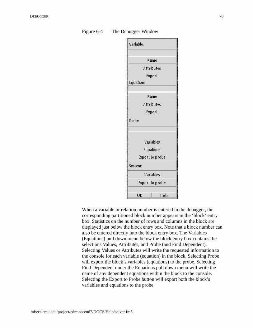
DEBUGGER 70
can
be
Figure 6-4 The Debugger Window
When a variable or relation number is entered in the debugger, thecorresponding partitioned block number appears in the ‘block’ entrybox. Statistics on the number of rows and columns in the block aredisplayed just below the block entry box. Note that a block number also be entered directly into the block entry box. The Variables(Equations) pull down menu below the block entry box contains theselections Values, Attributes, and Probe (and Find Dependent).Selecting Values or Attributes will write the requested information tothe console for each variable (equation) in the block. Selecting Prowill export the block’s variables (equations) to the probe. SelectingFind Dependent under the Equations pull down menu will write thename of any dependent equations within the block to the console.Selecting the Export to Probe button will export both the block’svariables and equations to the probe.
/afs/cs.cmu.edu/project/edrc-ascend7/DOCS/Help/solver.fm5

71 SOLVER
em,ortgger.et
te
theirnals
The debugger also responds to requests relating to the overall systor current solver instance. A Variables pull down menu and an Expto Probe button are located beneath the ‘System’ label on the debuThe Variables menu contains the selections Values, Attributes, ResValues, and Reset Nominals. Selecting Values or Attributes will writhe requested information to the console for each variable in thesystem. Selecting Reset Values will reset the system’s variables to nominal values. Selecting Reset Values will reset the system’s nomito their current variable values.
Last modified: June 20, 1998 10:32 pm

ny may
o
-
CHAPTER7 THE DATA PROBEWINDOW
7.1 OVERVIEW
Thedata probe shown in Figure 7-1 is a window which managescollections of names from the ASCEND simulation universe. Eachcollection is kept in a buffer, and the user can switch among as mabuffers as are needed for convenience. For example, the first bufferbe used as a set of bookmarks to store the names of interestingsubmodels within a large simulation, a second buffer can be used tmonitor a set of key variables, and a third can be used to monitorspecifications. The browser provides a two-level view of informationthe probe provides a random access view.(A new GIF is required forthis window -- the Help button is in the wrong place)

73 THE DATA PROBEWINDOW
theted,pe
and
es
e
e notme
h, the
Figure 7-1 Probe window
Names are imported to any collection buffer from the other parts ofuser interface or from a previously saved file of names. Once colleca name remains in the buffer until the user removes it, even if the tylibrary and simulations are deleted. This way the set of names ispreserved when the user makes a small modification to a MODEL rebuilds it.
Names in probe buffers are displayed with their corresponding valuor other attributes as appropriate. When a name is not well defined(perhaps because the simulation it came from has been deletedtemporarily) the attribute displayed is “UNCERTAIN.” As soon as thname becomes well-defined again by having a correspondingsimulation object built, the correct attribute will appear. Names ofatomic objects (reals, integers, sets, symbols, booleans) which havyet been assigned a value will be shown as “UNDEFINED” until sooperation assigns them a value.
7.2 THE FILE MENU
New buffer This starts another collection of names, which is initially empty. Eacbuffer receives a standard name when it is created, NoNameX.a4pwhere X is the number of the buffer. These buffer names appear atbottom of the File menu.
Last modified: June 20, 1998 10:32 pm

THE EDIT MENU 74
r’s
es,
ve
r
ols
nt
ioning.the
mes
ter
Read file This appends a file full of names into the current buffer and willautomatically attempt to associate them with the simulations in thesystem. This way the name list can be reloaded from a prior worksession. The file name is not associated with the buffer.
Save This will save the names in the current buffer to a file with the buffemenu name. If you wish to save with a more meaningful name, use“Save as.” Values are not saved with these names. To save the valuuse the Print command.
Save as This allows you to specify the directory and file name in which to sathe names in the current buffer.
Print This lets you print the current buffer to a printer or a file. This printswhat you see in the buffer window, including the values. The printesetup dialog will pop up for you to set the destination.
Close window Close this window. To reopen use the Data Probe tool under the Tomenu in the Script or select the PROBE button in the Toolbox.
Exit ASCEND Exit the ASCEND system. You will asked to verify that you really wato exit.
Buffer list You can create several different Probe buffers. A list of the buffersappears at the bottom of the File menu.
7.3 THE EDIT MENU
Highlight all Select all items in the displayed buffer.
Remove selectednames
This options removes all highlighted lines in the window. The selectin the probe can be set in a disjointed fashion using Ctrl while selectOne can select continguous items by dragging or by holding down Shift key when selecting the first and last item to be highlighted.
Remove allnames
This options removes all names in the current buffer window.
RemoveUNCERTAIN names
This removes all names that are not well defined. These are the nadisplayed as “name = UNCERTAIN.”
Copy This copies all the selected items in the current buffer to the compuclipboard. The items may then be pasted into any application thatsupports the clipboard -- for example, another ASCEND window, aFrame document and Excel.
/afs/cs.cmu.edu/project/edrc-ascend7/DOCS/Help/probe.fm5

75 THE DATA PROBEWINDOW
can.
en
owefaultved
er.
o the.
. The
f the
BEort use
u
7.4 THE VIEW MENU
Font Opens the window that lets you reset the fonts for this window. You select the type of font, the style (bold, etc.) and the size for the font
Openautomatically
Toggles a switch which, if set, will cause the Browser window to opwhenever anything is placed into it by an export command.
Save windowappearance
Saves the current settings for this window for font settings and windsize and placement on your computer screen. These become the dsettings for opening this window in the future. These settings are sain a .a4o text file for this window which the sytem stores in thesubdirectoryascdata in your “home” directory.
7.5 THE EXPORT MENU
to Browser This option sends the first selected name in the probe to the brows
to Display This options sends some form of the selected names in the probe tDisplay slave window, replacing whatever used to be in the display
7.6 THE PROBE FILTER
A class or classes of object can be imported to the probe en masseimport filter shown in Figure 7-2 lets you select which collection ofnames (probe buffer) is to receive the imported names which are otypes checked. Currently the probe filter window is accessible onlyfrom the Browser Export button.
The filtering import can also be executed from the Script using thePROBE command. The list of ones and zeros required for the PROcommand is ordered in the same way as the list of types in the impfilter window. The easiest way to set the list of ones and zeros is tothe Script recording feature and the Browser Export Many to probebutton.
7.6.1 THE HELP MENU
Brings up a text description of where to look for help on this window(i.e., it points to the pdf version of this document on the WWW.) Yomay, of course, look into the section mentioned in any local (butperhaps outdated) copy of the documentation.
Last modified: June 20, 1998 10:32 pm

THE PROBEFILTER 76
Figure 7-2 Probe import filter
/afs/cs.cmu.edu/project/edrc-ascend7/DOCS/Help/probe.fm5

77 THE DATA PROBEWINDOW
Last modified: June 20, 1998 10:32 pm

of
e
CHAPTER8 ASCPLOT
8.1 PLOT MAKER
The following contains a description of the options available in eachtheAscend Plot menus. TheAscend Plot window shown in Figure 8-1
Figure 8-1 The Ascend Plot Window
is a result of clicking on the ascplot button from the Toolbox with thleft mouse button.

79 ASCPLOT
t
omns.
t.ion,
8.1.1 THE EDIT MENU
From theEdit Menu, the following options are available when a dataset has not yet been loaded:Load data set andSelect grapher. TheSave data set, Unload data set, andMerge data sets options areavailable after one or more data sets have been loaded into the plowindow.
8.1.1.1 LOAD DATA SET
SelectingLoad data set opens theFile select box window. Thiswindow is used to select the file that contains the data generated frthe dynamic simulation. The default file is obs.dat. This file contaithe observation variables as set forth in the dynamic library modelsAfter having selected the appropriate file, press the OK button andreturn to theAscend Plot window.
8.1.1.2 SAVE DATA SET
This option is currently not functional.
8.1.1.3 UNLOAD DATA SET
By highlighting the desired data set and selectingUnload data setfrom theFile menu, the user can remove the data set from theAscendPlot window. TheDelete these data sets? window appears to verify thatthe user wants to remove the indicated data sets.
8.1.1.4 MERGE DATA SETS
8.1.1.5 SELECT GRAPHER
Currently, the only supported grapher is Xgraph (or its tk flavoredversion tkxgraph). Other possible graphers are XMGR and gnuploSince these graphers are not distributed with the ASCEND distributthey are also not supported.
8.1.2 THE EXECUTE MENU
To plot the variables in the plotted variables section, selectView plotfile from theExecute menu.
Last modified: June 20, 1998 10:32 pm

PLOT MAKER 80
.
addace.
erct
dedriate.g the
8.1.2.1 VIEW PLOT FILE
This option will plot the variables displayed in the plotted variablessection of theAscend Plot window.
8.1.2.2 WRITE PLOT FILE
To save the output in its graphical representation, selectWrite plot filefrom theExecute menu. Selecting this option opens theFile selectbox. Enter the name of the file to be saved and press the OK buttonThe default extension for the graph is .xgraph.
8.1.2.3 INSERT COLUMN
Selecting theInsert column option from theExecute menu opens theCreate Data window. This window is shown in Figure 8-2.
Figure 8-2 The Create Data Window
There are several options available from theCreate Data window.
8.1.2.3.1 Insert after Column
This can be any number between 0 and the maximum number ofvariables in the observation file. For example, if the user wishes to a column after the third column, the user should enter a 3 in this sp
8.1.2.3.2 Column type
The default value for Column type is data, however by placing thecursor over the data box and pressing the left mouse button, anothoption is reveiled. The other option is formula. The user should seledata if no formula can be used to describe the information to be adto the spreadsheet. The user should select formula if that is appropIn this case, a column was inserted after Column 0 and we are usinformula Column type.
/afs/cs.cmu.edu/project/edrc-ascend7/DOCS/Help/ascplot.fm5
81 ASCPLOT
eser themn
tion.e it
ts,
8.1.2.3.3 Formula
If the data option was selected in the previous section, then this donot apply. However, if the formula option was selected, then the uscan edit the default formula. The default formula takes the value ofvariable in the current row ($r) and the column before the new colu($c-1) and adds one (+1) to it.
8.1.2.3.4 Insert at end (overrides Column)
The user can select this box to place the new column after the lastcolumn in the spreadsheet. This will override anything in the Insertafter Column line.
8.1.2.3.5 Forget this insertion
The user can select this box to ignore the changes made to thespreadsheet.
8.1.2.4 RECALCULATE COLUMN
This option is currently not functional.
8.1.2.5 INSERT ROW
The insert row option has the same options as the Insert Column opNote that the formula take the value from the row immediately befor($r-1) and the current column ($c) and adds one (+1) to it.
8.1.2.6 RECALCULATE ROW
This option is currently not functional.
8.1.3 THE DISPLAY MENU
TheDisplay menu has various features which include showing andhiding the data in the spreadsheet, setting plot titles, loading old ploupdating existing plots, and deleting plots.
8.1.3.1 SHOW DATA / HIDE DATA
Selecting theShow data option from theDisplay menu loads the datainto the spreadsheet in the bottom section of theAscend Plot window.This option then toggles toHide data. Selecting this option will hidethe data just loaded into the spreadsheet section of the window.
Last modified: June 20, 1998 10:32 pm

PLOT MAKER 82
ber
set
tive.
tive.
les
thanse,
8.1.3.2 SET PLOT TITLES
Selecting theSet plot titles option from theDisplay menu opens theGraph Generics window. This window is shown in Figure 8-3.
Figure 8-3 The Graph Generics Window
There are several options within this window depending on the numof variables being plotted.
8.1.3.2.1 Plot Title
The user can change the default title (AscPlot) to something that ismore descriptive and meaningful for the given data. In this case, wethe title to be Composition Profile since we are plotting the molefractions of the components in the system.
8.1.3.2.2 X Axis Title
The user can change the default title (X) to something more descripIn this case, we are plotting the time on the x-axis.
8.1.3.2.3 Y Axis Title
The user can change the default title (Y) to something more descripIn this case, we are plotting the Composition on the y-axis.
8.1.3.2.4 Column # legend
In this case, (#) is the number of the variable being plotted. If variab2, 3, and 4 are being plotted, the will be entries in theGraph Genericswindow entitled Column 2 legend, Column 4 legend, and Column 4legend. These entries can be changed to something less descriptivethe default. Usually the default for this field is a bit much. In this cathe legend was changed to ‘a’, ‘b’, and ‘c’.
/afs/cs.cmu.edu/project/edrc-ascend7/DOCS/Help/ascplot.fm5

83 ASCPLOT
the(i.e.lore.
8.1.3.3 LOAD OLD PLOT
This option is currently not functional.
8.1.3.4 UPDATE PLOT
This option is currently not functional.
8.1.3.5 DELETE PLOT
This option is currently not functional.
The plot of the completed graph is shown in Figure 8-4.
Figure 8-4 Complete Plot
8.1.3.6 THE GRILL
The grill is located directly to the right of PLOT MAKER. Clicking onthis button with the left mouse button opens theXGraph Controlwindow. By clicking on the More button located at the bottom of thewindow, the user can scroll through numerous available options forgraphs. Some of these options include line color, fonts, graph type log or semilog), and marker types. These are left to the user to exp
Last modified: June 20, 1998 10:32 pm
NAVIGATION 84
f
t of.
leftble is
otted and
ase
ent
ine ofV)
on and)
thet the
ehe
8.2 NAVIGATION
Open a file using theLoad data sets option from theFile menu. Youwill notice that the selected file is now displayed in the top section otheAscend Plot window. By double-clicking on the file name with theleft mouse button, the observation variables are now placed in thesection entitled unused variables. The unused variables are the lisvariables that the user does not want to look at in the current graph
To select a variable to plot, highlight the desired variables using themouse button and click on the (>>) button. This will move the variafrom the unused variables list to the plotted variables list. Once thisdone, you can now plot the variable.
The two buttons separating the unused variabes section and the plvariables section are used to add (>>) and remove (<<) variables tofrom the plotted variables list.
You will notice that there is a section of theAscend Plot windowentitled Independent. Here the independent variable is time. This wset in the dynamic library file. If the user desires to look at the phasplot of two of the compositions, the user must move one of thecompositions into the Independent variable position.
To do this, let’s assume that all of the variables are currently in theunused variables list and we wish to plot the composition of compon‘c’ versus the composition of component ‘b’. Thus, component ‘c’ isnow going to be our independent variable. Highlight component ‘c’ the unused variables list and press the (V) button. This button is ontwo buttons located directly under the (>>) and (<<) buttons. The (button on the left is used to move variables between the unusedvariables list and the Independent variable list while the (V) button the right is used to move variables between the plotted variables listthe Independent variable list. Therefore, we are going to use the (Vbutton on the left.
By doing this, we see that the composition of component ‘c’ is now independent variable and the time is now an unused variable. Seleccomposition of component ‘b’ and press the (>>) button to move thvariable from the unused variables list to the plotted variables list. Tonly remaining task is to edit the plot title and axes using theSet plottitles option from theDisplay menu. Assuming we have done this asdescribed above, the resulting graph is shown in Figure 8-5.
/afs/cs.cmu.edu/project/edrc-ascend7/DOCS/Help/ascplot.fm5

85 ASCPLOT
The remaining section of theAscend Plot window is the HINT: section.This section contains a brief description of the various buttons andsections of the Ascend Plot window.
Figure 8-5 Phase Diagram
Last modified: June 20, 1998 10:32 pm

nd
g
rdo
CHAPTER9 DISPLAY SLAVE
9.1 OVERVIEW
The display slave window (Figure 9-1) functions as a dumping groufor information which is too complex to display in other ways in theLibrary, Browser or other primary windows. It has rudimentary editinabilities so the user can manually adjust the format of displayedinformation if needed, for example by rearranging a highly nonlinearelation with more than a few variables. Changes to displayed text not affect the rest of the system in any way.
Figure 9-1 Display slave window

87 DISPLAY SLAVE
n to a
sto
histo
r at
ode
g
ome
can.
9.2 DISPLAY FILE MENU
Print This option brings up the default print dialog described in the sectioUtilities. The print command can be used to save the displayed textfile.
Close window The option closes the display window.
Exit ASCEND Exit the ASCEND system. You will be asked to verify that you reallywish to exit ASCEND.
9.3 DISPLAY EDIT MENU
Cut Cut highlighted text to the computer paste buffer. You can paste thitext into any application that supports cut, copy and paste -- e.g., inFramemaker or Excel.
Copy Copy highlighted text to the computer paste buffer. You can paste ttext into any application that supports cut, copy and paste -- e.g., inFramemaker or Excel.
Paste Paste the contents of the computer paste buffer into the Scipt buffethe point of the cursor.
9.4 DISPLAY VIEW MENU
Show commentsin code
This option controls whether or not comments are displayed when cis displayedas read from source files. This setting is not retroactive;that is code already displayed will not be redisplayed when changinthis setting.
When code is displayed in the machine representation, i.e. withequations and set expressions in postfix (reverse polish) notation,comments are never displayed.
Save Displayoptions
Saves the current settings for this window for its options. These becthe default settings when opening this window in the future. Thesesettings are saved in a .a4o text file for this window which the sytemstores in the subdirectoryascdata in your “home” directory.
Font Opens the window that lets you reset the fonts for this window. You select the type of font, the style (bold, etc.) and the size for the font
Last modified: June 20, 1998 10:33 pm

TITLE LINE 88
en
owefaultved
dow.
o
u
next
Openautomatically
Toggles a switch which, if set, will cause the Browser window to opwhenever anything is placed into it by an export command.
Save windowappearance
Saves the current settings for this window for font settings and windsize and placement on your computer screen. These become the dsettings for opening this window in the future. These settings are sain a .a4o text file for this window which the sytem stores in thesubdirectoryascdata in your “home” directory.
9.4.1 FONT
This option brings up the standard font setting dialog so you canchange the size, style, and font of the characters in the display win
9.4.2 OPEN AUTOMATICALLY
This option controls whether or not the display slave window opensautomatically when it receives information. Sometimes it is easier tsend several items to the display and then open it at the end.
9.4.3 DISPLAY HELP MENU
Brings up a text description of where to look for help on this window(i.e., it points to the pdf version of this document on the WWW.) Yomay, of course, look into the section mentioned in any local (butperhaps outdated) copy of the documentation.
9.5 TITLE LINE
The title line at the bottom of the window is set by the last client toexport something to the display. The user may edit the title, but the time new information is displayed, these edits will be lost.
/afs/cs.cmu.edu/project/edrc-ascend7/DOCS/Help/display.fm5

89 DISPLAY SLAVE
Last modified: June 20, 1998 10:33 pm

tos.
I,useintene,sion.n also
e
y
t, as
CHAPTER10 ASCEND UNITS
10.1 THE MENU BAR
The Units Tool Set provides tools to allow the user to change thedisplay units for variables.
Units vsdimensions
We distinguish betweenunits anddimensions in ASCEND. Thedimensions of acceleration, for example, are L/T2, i.e., length/timesquared. Units for acceleration are: m/s2, ft/hr2 and so forth. A chapterin the Howto book tells you how to enter dimensioned equations inASCEND and includes a useful discussion on units and dimensionAlso see the ASCEND syntax document for a discussion.
Typical use The user will typically first pick the overall system of units such as SAmerican Engineering or cgs. Alternatively the user may select to thedefault display of units for some or all variable types. Displaying default units means ASCEND will present the units in terms of the basic dimensions supported by ASCEND (length, time, temperaturetc.). The user can select the units to be used for each basic dimenWhichever of these alternatives the user selects, he or she may thechoose the units ASCEND should use to display particular variabletypes. An example would be to select first SI units, then override thdisplay of energy to be in default units and pressure to be in atm.
Once users have created their favorite choices for display units, themay save them to files for later restoration.
We describe here the various tools available within the Units tool seseen in
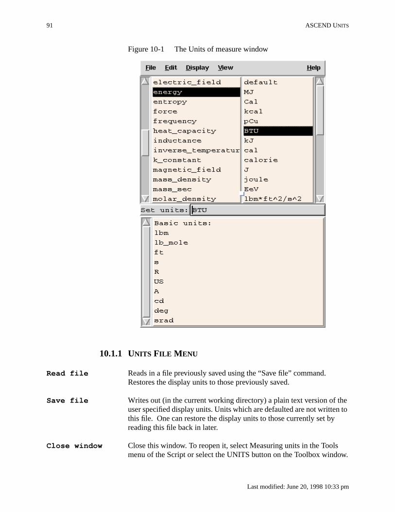
91 ASCEND UNITS
hen to
ow.
Figure 10-1 The Units of measure window
10.1.1 UNITS FILE MENU
Read file Reads in a file previously saved using the “Save file” command.Restores the display units to those previously saved.
Save file Writes out (in the current working directory) a plain text version of tuser specified display units. Units which are defaulted are not writtethis file. One can restore the display units to those currently set byreading this file back in later.
Close window Close this window. To reopen it, select Measuring units in the Toolsmenu of the Script or select the UNITS button on the Toolbox wind
Last modified: June 20, 1998 10:33 pm
THE MENU BAR 92
iongs a
ionsase
nitsay
can.
en
owefaultved
Exit ASCEND Exit the ASCEND system. You will be asked to verify that you reallywish to exit ASCEND.
10.1.2 UNITS EDIT MENU
Set precision Use the slider switch for this tool to set the number of digits ofprecision for displaying variable values to between 4 and 16. Precisis the number of digit displayed when the number is displayed usinscientific notation. For example, 0.12345678 e04 for 1234.5678 haprecision of 8 digits.
Set basic units Drops a cascading window in which are listed the ten basic dimensfor ASCEND. You can select in which units you wish to see each bdimenion to be displayed using this list.
10.1.3 UNITS DISPLAY MENU
Show all units Causes the Display window to open showing the extensive set of uconversions currently used in ASCEND. The list opens in the Displwindow.
10.1.4 UNITS VIEW MENU
SI(MKS) set Pushing this button makes the default display units SI units.
US Engineeringset
Pushing this button makes the default display units US Engineeringunits.
CGS set Pushing this button makes the default display units CGS units.
Font Opens the window that lets you reset the fonts for this window. You select the type of font, the style (bold, etc.) and the size for the font
Openautomatically
Toggles a switch which, if set, will cause the Browser window to opwhenever anything is placed into it by an export command.
Save windowappearance
Saves the current settings for this window for font settings and windsize and placement on your computer screen. These become the dsettings for opening this window in the future. These settings are sain a .a4o text file for this window which the sytem stores in thesubdirectoryascdata in your “home” directory.
/afs/cs.cmu.edu/project/edrc-ascend7/DOCS/Help/units.fm5

93 ASCEND UNITS
u
l becan
ithnits
icalnce
10.1.5 UNITS HELP MENU
Brings up a text description of where to look for help on this window(i.e., it points to the pdf version of this document on the WWW.) Yomay, of course, look into the section mentioned in any local (butperhaps outdated) copy of the documentation.
10.2 AN ESSAY ON UNITS VS DIMENSIONS
ASCEND stores all numbers in SI (MKS) units internally. The unitsassociated with a dimensionality (as exemplified by some atom) wilused when displaying variables of that dimensionality. These units be manipulated through the Units window.
Numbers with unrecognized dimensionality (higher derivatives,multipliers, residuals and what not) will be given units consistent wthe display units defined for the 10 base dimensions. The display ufor the 10 dimensions can be changed through the Units windowDisplay menu if you prefer an alternate default set such as USengineering, and so forth.
We recognize 10 base dimensions in the compiler:
L distance meter m
M mass kilogram kg
T time second s
E e- current ampere A
Q quantity mole mole
TMP temperature Kelvin K
LUM luminous intensity candela cd
P plane angle radian rad
S solid angle steradian srad
C currency currency CR
The units conversions are defined in $ASCENDDIST/compiler/units_input, which is not particularly restricted. Units_input isconverted to an efficient binary form (unitsfile.uni) at the timeASCEND is installed.
It can be argued that C is not a fundamental dimension, from a physstandpoint. There is more to life than physics: there is economy, heengineering, hence an Advanced System for Computations inENgineering Design.
Last modified: June 20, 1998 10:33 pm

AN ESSAY ON UNITS VS DIMENSIONS 94
eralner
g a
to
nits.
ty
alle
oftal
s.
he of
hich
ut
er
it
inge
The dimensions P and S are ‘supplementary’ according to the GenConference, but their use makes the coding of ASCEND much cleaand easier.
10.2.1 ON UNITS
The left box in the Units window lists a set of atom types, each havinunique dimensionality. Selecting an atom in the left box will fill theright box with different possible units that the system knows about display this type of variable. Dimensionless atoms and wilddimensioned atoms are not shown since they do not have display uIf you do not see an atom you expect here, it is because ASCENDalready found another atom of the same dimensionality, e.g. fugacimay show up instead of pressure.
Selecting a unit in the right box sets that unit as the display unit forvariables having the same dimensionality of the selected atom in thleft box. Thus pickingatm for fugaciy will also change pressure unitsto atm. Selecting ‘default’ will cause the display to be a combinationthefundamental units (a nice way to remind oneself of the fundamenunits for energy, for example).
Fundamental units are the units corresponding to single dimensionThese units are chosen on the Display menu under the dimensionchoices. No atoms with fundamental units are listed in the left box. Tcurrent set of fundamental units is always shown at the very bottomthe units window. This set is used whenever a value is displayed wdoes not have a user specified units set associated with itsdimensionality. The fundamental units are created via the units_inpfile mentioned above. If you do not find one you want, ask whoevercompiled your version of unitsfile.uni to add the missing unit andrebuild the unitsfile.uni.
If converting the units for a variable makes the display of that numbimpossible (e.g., due to overflow). ASCEND will first attempt todisplay it using its fundamental units. If it still cannot be displayed, will be displayed in SI units.
You may specify a new combination of existing units (e.g. Pa*s) ustheSet units which is the line at the bottom of the window. Type in thcombination desired and press RETURN.
Unit strings may not have parentheses in them. For example, kg/(m*s^2) is not allowed.
/afs/cs.cmu.edu/project/edrc-ascend7/DOCS/Help/units.fm5

95 ASCEND UNITS
Last modified: June 20, 1998 10:33 pm

e
ets
CHAPTER11 THE ASCEND TOOLBOX
Thetoolbox window shown in Figure 11-1 lets the users open and closthe various windows for the tool sets available in ASCEND. Thetoolbox window is a vertical window containing 12 buttons: exit,ascplot, help, utilities, bug report, LIBRARY, BROWSER, SOLVER,PROBE, UNITS, DISPLAY, SCRIPT.
The buttons in the toolbox with names in ALL CAPS (LIBRARY andfollowing) open and close the windows for the corresponding tool s
Figure 11-1 The ASCEND Toolbox window.
97 THE ASCEND TOOLBOX
we
to betton.
l the
nd is
for
thatesedool.
in ASCEND1. As each of these toolsets has its own documentation,shall not discuss them here. We discuss here only the first set ofbuttons: Exit, Ascplot, Help, Utilities, and Bug Report.
1. The more advanced user should note that changing the iconname of a window (viaascend.ad) does not change its toolbox name.
11.1 EXIT
This button shuts down all of ASCEND after making sure you wantquit. ASCEND does no checking to see if there is unsaved work socertain you have saved what you want of it before selecting this bu
(For more advanced users, we note that, just before exiting, we caltcl function user_shutdown which may be redefined in the.ascendrc file in your HOME directory. Under Windows, the_ascendrc is the name of the corresponding file.)
11.2 ASCPLOT
Selecting this button opens the plotting tool for ASCEND. You can fiany file that contains data for a plot and plot it with this tool. Ascplotdescribed elsewhere.
11.3 HELP
Pressing this button will provide access to the Help DocumentationASCEND. The help system is described elsewhere.
11.4 UTILITIES
Selecting this button opens the system utilities window. The systemutilities window is described elsewhere.
11.5 INTERNALS
The internals window gives catalog access to the global Tcl arrays maintain and control the GUI and other ASCEND options. It also givaccess to the list of ASCEND functions (C callbacks) that are definand their built-in documentation. Casual users should not use this t
Last modified: June 20, 1998 10:33 pm
BUG REPORT 98
we
r
dt
er
ve
ug
ot
to
11.6 BUG REPORT
The linkhttp://www.cs.cmu.edu/~ascend/Email.htmlis connected to the web server for ASCEND at CMU. Alternatively,send a bug report [email protected] you cannot access this link. We do not have an 800 number, but usually get to bug reports very quickly.
When submitting a bug report, please try to
1. Duplicate the error.
2. Tell us in excruciating detail how you duplicated it.
3. Report to us the platform and operating system (OS) on whichyou are running. Also please tell us the distribution number fothe ASCEND code on which you are running. This is researchsoftware. We are not committed to backward compatibility, anwe do not have access to all the platform/OS combinations outhere. If the bug you report has been fixed in a newer version,your only fix is to get the new version or fix it yourself. If you aron a platform to which we do not have access, we will consideworking out the bugs with you in the hope that you will then gius back a copy for the new platform.
4. Send along any model code you have that is involved in the bmanifestation. It may happen that, in the process of fixing theASCEND bug, we could fix some of your model bugs. We are nin the business of debugging your model code unless it is alsointeresting to our research. We often find new applications ofASCEND interesting, however.
5. Subscribe to the ASCEND user mailinglist/bboard: Send [email protected] .
/afs/cs.cmu.edu/project/edrc-ascend7/DOCS/Help/toolbox.fm5

99 THE ASCEND TOOLBOX
Last modified: June 20, 1998 10:33 pm

D
nt,
ites
CHAPTER12 THE SYSTEM UTILITIES WINDOW
12.1 OVERVIEW
Thesystem utilities window shown in Figure 12-1 displays and allowsmodification of the variables which control the interaction of ASCENwith the operating system and with other programs.
The values of the variables are initialized from the user’s environmefrom the file.ascend-config in the user’s HOME directory, andfrom settings within ASCEND.
If the user chooses to save the system utility settings, ASCEND wrthe current values of the variables into file.ascend-config in theuser’s HOME directory. ASCEND will automatically reread thosevalues in the next time it starts.
Figure 12-1 The System Utilities window manages ASCEND’sinteraction with the operating system and with otherprograms.

101 THE SYSTEM UTILITIES WINDOW
is
s
tely
wns
Wds
er,
lpin a
to
When working with the system utilities window, it is important toremember that changes to the variables propagateimmediatelythroughout ASCEND, and that there is no way to undo or cancelchanges made to the variables1.
1. Some variables can be restored to the values in effect the last time the system utilities were saved, but thonly works if the user has previously saved the values, and it does not restore every variable.
12.2 VARIABLES
The system utilities window contains the following settings. Settingmarked with an asterisk* are not saved in.ascend-config .
To change a variable’s value, click in the box to the right of thevariable’s label and type the new value. This new value is immediaavailable to the ASCEND system.
12.2.1 WWW ROOT URL
ASCEND distributes its help system as HTML documents, and spaa web browser to view these documents. The variable WWW RootURL gives the root of the ASCEND help tree, and the variables WWRestart Command and WWW Startup Command contains commanto connect to a running web browser and to start a new web browsrespectively.
WWW Root URL contains the first part of a URL to the ASCEND hetree; it is not necessarily a complete URL. The variable should end forward slash (/). TheHelp menus and buttons in ASCEND willappend text to this value and invoke WWW Restart Command orWWW Startup Command with the complete URL.
The person who installs ASCEND at a site should set this variable the root of the directory containing that site’s copy of the ASCENDhelp files, for example:file://localhost/usr/local/lib/ascend/help/at CMU ICES.
The valuehttp://www.cs.cmu.edu/~ascend/help/will connect you to the help pages at the ASCEND web site.
Last modified: June 20, 1998 10:33 pm

VARIABLES 102
eb
up
this
d
d is
code.
d
e
ent
he
12.2.2 WWW RESTART COMMAND
This is a command to redirect the attention of your already running wbrowser to a new URL. If this command returns an error code,ASCEND will attempt to start a new browser using the WWW StartCommand.
If your favorite browser does not support restarting, set the value of variable tofalse . This will cause a new browser to start for everyhelp query from the ASCEND interface.
ASCEND will replace every occurrence of%U in this command withthe URL to be viewed. The default value of WWW Restart Commanisnetscape -remote openURL(%U)
12.2.3 WWW STARTUP COMMAND
This is a command to start your favorite web browser. This commaninvoked if the value of WWW Restart Command isfalse or ifattempting to start a browser using that command returns an error
ASCEND will replace every occurrence of%U in this command withthe URL to be viewed. The default value of WWW Startup Commanisnetscape %U
12.2.4 ASCENDLIBRARY PATH *
The ASCENDLIBRARY variable contains a list of directories that thLibrary and Script tools search to find files containing ASCENDmodels and scripts.
The format of the directory list should resemble the PATH environmvariable for your platform: a colon (:) separated list of directories(using forward slashes) on UNIX, a semicolon (;) separated list ofdirectories (using backward slashes) on Windows.
The ASCENDLIBRARY variable is initialized from the user’senvironment or from the ASCEND binary; its value is not saved in tuser’s.ascend-config file.
/afs/cs.cmu.edu/project/edrc-ascend7/DOCS/Help/utilities.fm5
103 THE SYSTEM UTILITIES WINDOW
atforeanteast
then in
f
,
12.2.5 SCRATCH DIRECTORY
The scratch directory is used to write the temporary and plot files thASCEND creates. The temporary files are automatically deleted beyou leave ASCEND, but the plot files are not (since people often wto save plots). You should periodically remove any plot files from thscratch directory, else you may slow build up a large collection of pplot files.
Any existing directory you have write access to can be used as thescratch directory. Under UNIX,/tmp is the default value of the scratchdirectory. Under Windows, the directory given in the environmentvariable TEMP, TMP, or TMPDIR is used as the default value.
12.2.6 WORKING DIRECTORY
Typically, this is the directory you start ASCEND from, but it can beany existing directory you have write access to. Our handling of theworking directory is a bit “flaky” at the moment because ASCEND’scommand line allows the user to change directories without telling rest of the interface about it. Intermediate files are sometimes writtethe working directory.
12.2.7 PLOT PROGRAM TYPE
Currently, the only supported plot types isxgraph plot(abbreviatedxgraph ). This setting tells the plot window what type oplot file it should generate.
12.2.8 PLOT PROGRAM NAME
This is the name of your plotting program. It should accept the plottype listed in Plot Program Type as input.
The default isxgraph on UNIX andtkxgraph on Windows. Bothxgraph and tkxgraph are available from the ASCEND web site:http://www.cs.cmu.edu/~ascend/
12.2.9 TEXT EDIT COMMAND
This is a command to spawn your favorite text file editor. (Currentlynothing in ASCEND invokes this command.)
The default isemacs on UNIX andrunemacs on Windows.
Last modified: June 20, 1998 10:33 pm

VARIABLES 104
rite
box.g,
ofe
log ifsion.
es
ry
12.2.10 POSTSCRIPT VIEWER
This is a command to spawn a program for viewing Postscript files.(Currently, nothing in ASCEND invokes this command).
The default isghostview on UNIX and on Windows.
12.2.11 SPREADSHEET COMMAND
This is a command to spawn your favorite spreadsheet program.(Currently, nothing in ASCEND invokes this command2).
2. Nothing invokes this command because there is no ASCEND code that supports it. Someone needs to wcode that will write out the desired variables as columns of numbers suitable for importing into anyspreadsheet. If you want to be that someone, let us know and we’ll be happy to consult. We have somepseudocode for this already; contact us [email protected] .
12.2.12 TEXT PRINT COMMAND
This entry displays the last command generated by the print dialog Changing the value of this entry will have no effect on future printinsince the print dialog manages all aspects of printing.
This value is displayed here as a hold-over from previous versions ASCEND; developers sometimes use it as a check to make sure thprint dialog is doing the right thing.
12.2.13 PRINTER VARIABLE *
This entry displays the last printer the user selected in the print diabox, or the value of the PRINTER or LPDEST environment variablethe user has not used the print dialog box during this ASCEND ses
Changing the value of this entry will have no effect on future printing3,since the print dialog manages all aspects of printing.
This value is not saved in the user’s.ascend-config file.
3. This is not entirely true. This entry will change the value of the PRINTER environment variable (but not thLPDEST environment variable). Any command you invoke from ASCEND command prompt that dependon the PRINTER environment variable will use the value displayed in this entry.
12.2.14 ASCENDDIST DIRECTORY *
The value of the ASCENDDIST environment variable is the directocontaining the installed ASCEND distribution. If a user can see this
/afs/cs.cmu.edu/project/edrc-ascend7/DOCS/Help/utilities.fm5

105 THE SYSTEM UTILITIES WINDOW
ect.
on
nt
ry
on
t
on
t
ow
variable inside the system utilities window, it means its value is corrChanging the value will most likely cause things to break.
The person who installs ASCEND at a site is typically the only perswho needs to be concerned with its value.
The ASCENDDIST variable is initialized from the user’s environmeor from the ASCEND binary; its value is not saved in the user’s.ascend-config file.
12.2.15 TCL_LIBRARY ENVIRONMENT VARIABLE *
The value of the TCL_LIBRARY environment variable is the directocontaining the installed*.tcl files required by Tcl. If a user can seethis variable inside the system utilities window, it means its value iscorrect. Changing the value will most likely cause things to break.
The person who installs ASCEND at a site is typically the only perswho needs to be concerned with its value.
The TCL_LIBRARY variable is initialized from the user’s environmenor from the ASCEND binary; its value is not saved in the user’s.ascend-config file.
12.2.16 TK_LIBRARY ENVIRONMENT VARIABLE *
The value of the TK_LIBRARY environment variable is the directorycontaining the installed*.tcl files required by Tk. If a user can seethis variable inside the system utilities window, it means its value iscorrect. Changing the value will most likely cause things to break.
The person who installs ASCEND at a site is typically the only perswho needs to be concerned with its value.
The TK_LIBRARY variable is initialized from the user’s environmenor from the ASCEND binary; its value is not saved in the user’s.ascend-config file.
12.3 BUTTONS
The actions associated with the buttons on the system utilities windare:
Last modified: June 20, 1998 10:33 pm
BUTTONS 106
.
may.
g
y
12.3.1 OK
This button closes the system utilities window. Closing will fail if thescratch directory and working directory are not writable by the user
12.3.2 SAVE
This button writes the current value of most of the variables in thesystem utilities window to a file called.ascend-config in yourHOME directory4. ASCEND will read this file on startup to get yourpreferred values.
The variables whose names are in ALL CAPS (i.e.,ASCENDLIBRARY, PRINTER, ASCENDDIST, TCL_LIBRARY,TK_LIBRARY) arenot saved to.ascend-config . These areenvironment variables that are set as part of the login process. Youchange them interactively, but their interactive values are not saved
4. Under Windows, you can set your HOME directory by setting the HOME environment variable by openinthe Control Panel, double clicking the System icon, clicking the Environment tab, and adding the HOMEvariable to the list of user environment variables.
12.3.3 READ
The button causes the system utilities window to reread the valuesstored in.ascend-config in your HOME directory. This is usefulfor editing.ascend-config outside of ASCEND while runningASCEND, or for verifying that the changes you saved were properlsaved.
12.3.4 MORE
The button rotates you through the pages of options.
12.3.5 HELP
The button should direct your web browser to this document.
/afs/cs.cmu.edu/project/edrc-ascend7/DOCS/Help/utilities.fm5

107 THE SYSTEM UTILITIES WINDOW
Last modified: June 20, 1998 10:33 pm

ce
ons
CHAPTER13 FONT SELECTION DIALOG
13.1 OVERVIEW
Thefont selection dialog (Figure 13-1) is used to select the font for thewindow from which it is opened. There is no way through the interfato change the font for every ASCEND window.
Currently, the fonts you select are not remembered across invocatiof ASCEND. This is a feature we will be adding in a future release.
Figure 13-1 The font selection dialog.

109 FONT SELECTION DIALOG
ont
is
ontcang
stt to
a,
ow.
rnt
ng
the
To change the default fonts for ASCEND, see Setting the Default Flater in this chapter.
The font which the font selection dialog displays when it is opened independent of the current window’s font. This is actually a feature.When you close the font selection dialog (by pressing either the OKButton or the Cancel Button) and reopen it, it will display the same fas when it was closed. This way, once you find a font you like, you change other ASCEND windows to this same font by simply openinthe font selection dialog and pressing OK. As a default, the very firtime you open the font dialog in an ASCEND session, the font is seCourier 12 normal .
The font selection dialog has eight parts: Font Menu, Style Menu,Cancel Button, OK Button, Current Font Sample, Font Sampler ArePoint Size Slider, Current Font Selection.
13.2 FONT MENU
The Font menu displays the fonts available for your platform (e.g,Helvetica, Courier). Selecting one of these fonts will update theCurrent Font Sample and Current Font Selection areas of the wind
13.3 STYLE MENU
The Style menu allows you to specify attributes (e.g., Bold, Italic) fothe selected font. As you add and remove attributes, the Current FoSample and the Current Font Selection will reflect the changes.
13.4 CANCEL BUTTON
The Cancel button closes the font selection window without changithe fonts of the window.
13.5 OK BUTTON
The OK button closes the font selection window and sets the font ofwindow to the font listed in the Current Font Selection area.
Last modified: June 20, 1998 10:33 pm

CURRENTFONT SAMPLE 110
nt,
l be
ntse
yed
, but
d to
e of
y
13.6 CURRENT FONT SAMPLE
This area of the font selection window shows a sample of text in fostyle, and size you have currently selected.
If you want to see what your current selection does to particularcharacters, you may type into this area. Note that your additions wildeleted when you change any aspect of the font (style, size, font).
13.7 FONT SAMPLER AREA
This area of the font selection window shows you a sample of the foavailable for your platform. You may make one of the listed fonts thcurrent selection by clicking the font with the left mouse button. Thecurrently selected styles and sizes remain in effect.
13.8 POINT SIZE SLIDER
This slider lets you choose the point size of the font. The text displain the Current Font Sample updates immediately.
13.9 CURRENT FONT SELECTION
This area displays the Tcl name for the font (including the size andstyle(s)) that you have currently selected. You may type in this areadoing so will have no effect on the font.
13.10 SETTING THE DEFAULT FONT
To have ASCEND use the same font each time you run it, you needo the following steps.
1. Use the font selection dialog to choose a font you like. Make anote of the Tcl name for the font; this name is displayed in theCurrent Font Selection area of the window.
2. Open the system utilities window and make a note of the valuASCENDDIST.
3. Exit ASCEND.
4. Under the ASCENDDIST directory, there should be a director
/afs/cs.cmu.edu/project/edrc-ascend7/DOCS/Help/fontsel.fm5

111 FONT SELECTION DIALOG
stt
ethe
t.
calledTK, and in this directory a file calledascend.ad . Copythis file to your HOME directory1 and name it.ascend.ad 2.
5. Add the following lines at the end of.ascend.ad , replacingcourier 11 normal with the font you noted in Step 1.
Global font courier 11 normal
Global labelfont courier 11 normal
Toolbox font courier 11 normal
Library font courier 11 normal
Display font courier 11 normal
Browser font courier 11 normal
Probe font courier 11 normal
Units font courier 11 normal
Script font courier 11 normal
Solver font courier 11 normal
Debugger font courier 11 normal
6. Save.ascend.ad , and restart ASCEND.
Note that this file also contains the default size and position for moASCEND windows. To change the position or size of a window, edithe lines containinggeometry ; the format for the geometry isWWxHH+xx +yywhereWW is the width of the window,HH is its height,xx is thedistance between the left edge of the screen and the left edge of thwindow, andyy is the distance between the screen’s top edge and window’s top edge.
1. To set your HOME directory under Windows, open the Control Panel, double click the System icon, selecthe Environment tab, and set the HOME environment variable to a directory you want to consider “home”
2. Under Windows, the name_ascend.ad also works.
Last modified: June 20, 1998 10:33 pm

CHAPTER14 THE PRINT DIALOG
14.1 OVERVIEW
Theprint dialog shown in Figure 14-1 allows the user to modify thesettings which control the printing of information from withinASCEND.
14.2 SETTINGS
14.2.1 DESTINATION
This is a pop-up menu that allows you to select one of the followingoptions for printing: Print, Write to file, Append to file, Enscript, orCustom.
Figure 14-1 The print dialog.

113 THE PRINT DIALOG
e
his
e
file
14.2.1.1 PRINT
On UNIX machines, this option sends the window’s contents to theprinter specified in the Printer field (PRINTER). Under SystemVsystems1, the commandlp -d PRINTERis used as the interface to the printer; on all other UNIX systems, thcommandlpr -P PRINTERis used.
Under Windows, the commandnotepad /pis used to send the window’s contents to the user’s default printer. Twill not print the Matrix display and other graphic displays correctlybecause those generate PostScript. Text windows (Display, Probe,Script, Library) will print correctly.
1. HP-UX, SGI IRIX, and Solaris 2.x.
14.2.1.2 WRITE TO FILE
Under UNIX, this option writes the contents of the window to the fillisted in the Name of file field. If a file with the same name exists,ASCEND will overwrite the file after verifying that the user wants tooverwrite the file.
This option is not available on the Windows platform.
This option is another version of Save As and will likely go away infuture releases of ASCEND.
14.2.1.3 APPEND TO FILE
Under UNIX, this option appends the contents of the window to the listed in the Name of file field. If the file does not exist, it will becreated.
This option is not available on the Windows platform.
This option will likely go away in future releases of ASCEND.
14.2.1.4 ENSCRIPT
On UNIX, this option uses theenscript program to queue thewindow’s contents to the printer specified in the Printer field
Last modified: June 20, 1998 10:33 pm

SETTINGS 114
cript
e
.
ite
(PRINTER). On SystemV systems, the commandenscript -d PRINTER enscript-flagsis used; on all other UNIX systems, the commandenscript -P PRINTER enscript-flagsis used. The value of enscript-flags is the value specified in the Ensflags field.
This option is not available on the Windows platform.
14.2.1.5 CUSTOM
This option allows the user to specify a custom print command. Thuser should type their custom command in the User print commandfield; the command should accept a file name as its final argument
This option is not available on the Windows platform.
14.2.2 PRINTER
Under UNIX, this field specifies the printer to send the document towhen the Destination is Print or Enscript.
This field has no effect under Windows.
14.2.3 NAME OF FILE
Under UNIX, this field contains the name of the file used by the Wrto file and Append to file options.
This field has no effect under Windows.
14.2.4 ENSCRIPT FLAGS
Under UNIX, this field contains the options sent to theenscriptprogram when the Destination is Enscript.
This field has no effect under Windows.
14.2.5 USER PRINT COMMAND
Under UNIX, this field contains the command used to “print” thewindow’s contents when the Destination is Custom. This commandshould accept the name of a file (a temporary file containing thecontents of the window) as its final argument.
/afs/cs.cmu.edu/project/edrc-ascend7/DOCS/Help/print_dialog.fm5

115 THE PRINT DIALOG
es
s and
This field has no effect under Windows.
14.3 BUTTONS
14.3.1 OK
Pressing this button accepts the settings, sends the document to thprinter or to the specified file, and closes the print dialog. The valuedisplayed in the Text print command and the PRINTER fields in thesystem utilities window will change to reflect the new settings.
14.3.2 HELP
Pressing this button should cause your web browser to display thisdocument.
14.3.3 CANCEL
This button ignores any changes you may have made to the settingcloses the print dialog. The file is not printed.
Last modified: June 20, 1998 10:33 pm
we a
NDadily
e
er inD,tl
n, altere
orthe
heet
CHAPTER15 SOLVED SIMPLE MODELING
PROBLEMS WITHASCEND
In this chapter we present two simple modeling problems for whichthen show you our ASCEND models for solving them. Modeling ismatter of style, and we will start to show you what we believe to begood styles for modeling. We assume you have not used the ASCEsystem before. These problems are very generic and should be refollowed by anyone with a modest technical background.
One purpose is to show you some of the different ways you can usASCEND. Specifically we want to show you that you can useASCEND to setup and solve the simple types of problems that youmight have solved using a spreadsheeting program. Indeed, we usASCEND to solve homework problems quite often. When you factothe powerful debugging tools, you might find it faster to use ASCENespecially as the models get more complex. And no one would wan(we think) to solve a 20,000 simultaneous nonlinear equation modeusing a spreadsheeting program.
A major advantange of using ASCEND is that once you have writtedebugged and learned to solve such a model, you can interactivelythe "fixed" flags for the variables, changing which variables are to bfixed and which to be calculated. You can then immediately solve optimize the new problem, using the previously solved problem as initial guess.
15.1 ROOTS OF A POLYNOMIAL
In this problem you wish to find the roots of a polynomial. Assumeyou do not wish to keep the code. You could readily use a spreads

117 SOLVED SIMPLE MODELING PROBLEMS WITHASCEND
ut
ex,
ingotre to
ce
ctly,
le, a
the
fail is aes
er, and
program with its "root finder" routine to solve this type of problem, byou can as readily use ASCEND.
15.1.1 PROBLEM STATEMENT
Numerically compute the roots of(x-1)(x-5)(x+7)(x2+1) =0. (Given inthis form the roots are obviously 1, 5, and -7. Two roots are compland ASCEND will not find them.)
15.1.2 ANSWER
You can find the roots by guessing initial points after typing in, loadand compiling the following model. You would use any text editor tenter this model into the computer. If you use a "WYSIWYG" (whayou see is what you get) editor such as Word or Framemaker, be susave the file as atext only file. If possible, use a simpler text editor.
MODEL polynomial_roots; 1
x IS_A generic_real; 2
(x-1)*(x-5)*(x+7)*(x^2+1) = 0; 3
END polynomial_roots; 4
This simple model is a stand-alone model. You need no otherpredefined libary models to support it. Load and compile an instanof this model (using tools in the LIBRARY tool set), browse it (usingthe BROWSER tool set) to see if it appears to have compiled correand then pass it to the SOLVER tool set.
This model involves a single equation in the single unknown variabx. The ASCEND solver treats a single equation in one unknown inspecial manner when asked to solve it. The solver first attempts torearrange the equation by simple algebraic manipulations to isolateunknown on the left hand side of the equation in the form x =expression not involving x. In this form, solving is simply evaluatingthe expression on the right hand side once. Here the solver wouldas there is no way to isolate x on the left hand side as the equationfifth order polynomial in x. When rearrangement fails, the solver usbisection to locate a root in the range between the lower and upperbound on the variable. You can see the bounds, x.lower and x.uppusing the BROWSER. The default values for these bounds are plusminus 1020 respectively, which gives a very large range in which to
Last modified: June 20, 1998 10:33 pm

NUMERICAL INTEGRATION OF TABULAR DATA 118
root
toeting
e
seth
e
o a
onds.
look for the root. You should change the bounds1 to more realisticones. Selecting bounds to be -10 to 0 and then solving will find the x=-7. Selecting other values will find the other roots.
This model illustrates that you can quickly set up and solve simpleproblems using ASCEND. Note that you would have been requiredplace bounds on x had you used a goal seeking tool in a spreadsheprogram if you wanted to control which root to locate.
1. To set the value for a variable interactively, select the variable when it is display in the right window or in thlower window with the RIGHT mouse button (the other button). A window for changing its value opens.
15.2 NUMERICAL INTEGRATION OF TABULAR
DATA
This problem is similar to the previous one in that it is very easy to up and solve. It adds in the notion of units (e.g., ft, m, hr, atm) whicASCEND handles in a straight-forward manner, relieving modelersfrom thinking about converting among the many units they might uswhen expressing the data for a problem.
Again we are talking about producing throw-away code. All we arereally concerned with here is the answer which we intend to put intreport. We are using ASCEND as a "calculator."
15.2.1 PROBLEM STATEMENT
Given the following velocity data vs. time, estimate numerically thedistance one has traveled between time equal to zero and 100 sec
Table 1: Velocity data to be integrated
data pointnumber
time,s
velocity,ft/min
1 0 100
2 10 120
3 20 130
4 30 135
5 40 140
6 50 160
7 60 180
/afs/cs.cmu.edu/project/edrc-ascend7/DOCS/Help/simple_problems.fm5
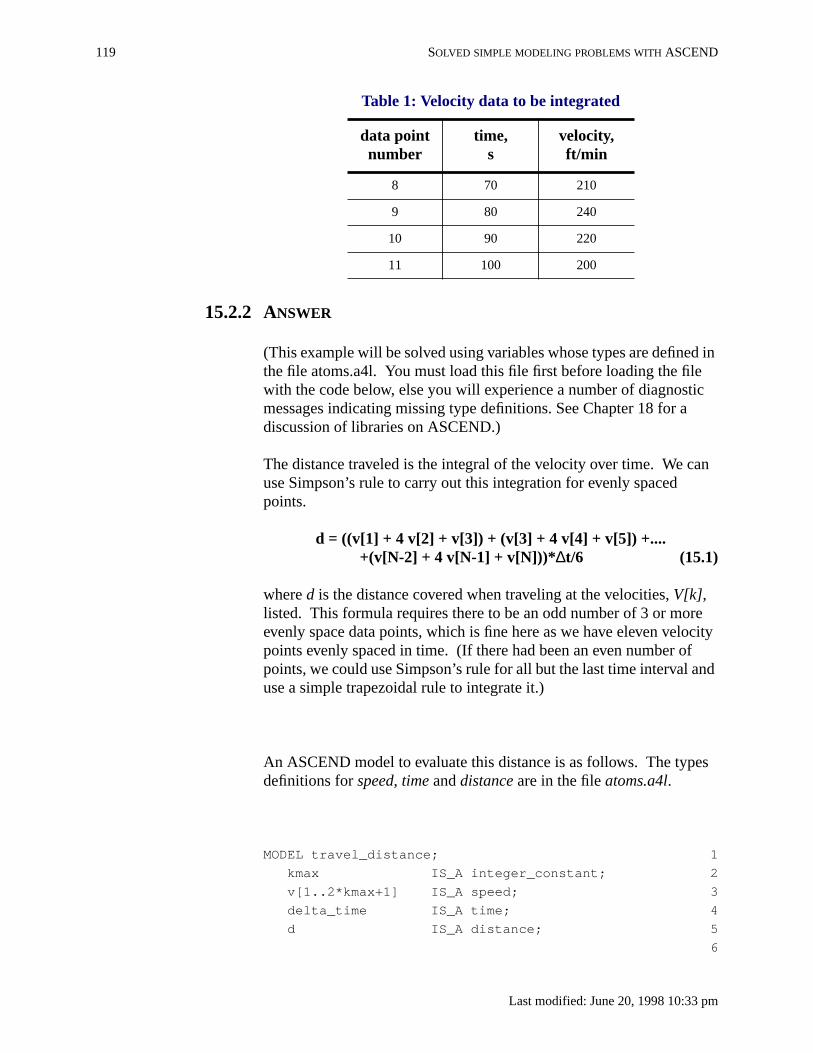
119 SOLVED SIMPLE MODELING PROBLEMS WITHASCEND
d in
ic
an
reocityfnd
es
15.2.2 ANSWER
(This example will be solved using variables whose types are definethe file atoms.a4l. You must load this file first before loading the filewith the code below, else you will experience a number of diagnostmessages indicating missing type definitions. See Chapter 18 for adiscussion of libraries on ASCEND.)
The distance traveled is the integral of the velocity over time. We cuse Simpson’s rule to carry out this integration for evenly spacedpoints.
d = ((v[1] + 4 v[2] + v[3]) + (v[3] + 4 v[4] + v[5]) +....+(v[N-2] + 4 v[N-1] + v[N]))*∆t/6 (15.1)
whered is the distance covered when traveling at the velocities,V[k] ,listed. This formula requires there to be an odd number of 3 or moevenly space data points, which is fine here as we have eleven velpoints evenly spaced in time. (If there had been an even number opoints, we could use Simpson’s rule for all but the last time interval ause a simple trapezoidal rule to integrate it.)
An ASCEND model to evaluate this distance is as follows. The typdefinitions forspeed, time anddistance are in the fileatoms.a4l.
MODEL travel_distance; 1
kmax IS_A integer_constant; 2
v[1..2*kmax+1] IS_A speed; 3
delta_time IS_A time; 4
d IS_A distance; 5
6
8 70 210
9 80 240
10 90 220
11 100 200
Table 1: Velocity data to be integrated
data pointnumber
time,s
velocity,ft/min
Last modified: June 20, 1998 10:33 pm

NUMERICAL INTEGRATION OF TABULAR DATA 120
in ft/
this
g SI
d = SUM[v[2*k-1]+4*v[2*k]+v[2*k+1] SUCH_THAT k IN
[1..kmax]]*delta_time/6; 7
END travel_distance; 8
9
MODEL test_travel_distance REFINES travel_distance; 10
kmax :== 5; 11
12
METHODS 13
METHOD specify; 14
v[1..2*kmax+1].fixed := TRUE; 15
delta_time.fixed := TRUE; 16
END specify; 17
18
METHOD values; 19
v[1] := 100 {ft/min}; 20
v[2] := 120 {ft/min}; 21
v[3] := 130 {ft/min}; 22
v[4] := 135 {ft/min}; 23
v[5] := 140 {ft/min}; 24
v[6] := 160 {ft/min}; 25
v[7] := 180 {ft/min}; 26
v[8] := 210 {ft/min}; 27
v[9] := 240 {ft/min}; 28
v[10] := 220 {ft/min}; 29
v[11] := 200 {ft/min}; 30
delta_time := 10 {s}; 31
END values; 32
END test_travel_distance; 33
If you look carefully at this model, you will note that we did NOTaccount for the conversion factors required because velocities are min while the time increment is in seconds. ASCEND understandsthese units and makes all the needed conversions. When you run model, you can ask for the distance to be displayed to you in anysupported length units you would prefer (e.g., ft, mile, m, cm,angstroms, lightyears). The distance traveled, when reported usinunits, is 42.84 m.
/afs/cs.cmu.edu/project/edrc-ascend7/DOCS/Help/simple_problems.fm5

121 SOLVED SIMPLE MODELING PROBLEMS WITHASCEND
Last modified: June 20, 1998 10:33 pm

THE WHEN STATEMENT 122
oll
ich
tain
nt
CHAPTER16 A CONDITIONAL MODELING
EXAMPLE: REPRESENTING A
SUPERSTRUCTURE
To give an example of the application of the conditional modeling toin ASCEND -theWHEN statement-, we developed a simplified modefor the superstructure given in Figure 16-1. The code listed belowexists in a file in the ASCEND models subdirectory entitledwhen_demo.a4c. You could run this example by loading this file andusing it and its corresponding scriptwhen_demo.a4s.
16.1 THE WHEN STATEMENT
Before showing the example, we want to start by giving a briefexplanation about the semantics of the WHEN statement, a tool whallowsASCEND to represent conditional models efficiently.
In theWHEN statement, we take advantage of the fact thatASCEND isbased on object oriented concepts where model definitions can conparts that contain parts to any level. Furthermore, inASCEND, a simple
Figure 16-1 Superstructure used in the example of the application of the when stateme
f1
f2
c1
co1 h1
r2
r1
co2 fl1
h2
h3
c2
Feed 1 (cheap)
Feed 2(exp.)
Pby
<1000ton/day
>90 %pure C
high conv, high cost
low conv, low cost
A + B Cs1
sp1s2
m1
/afs/cs.cmu.edu/project/edrc-ascend7/DOCS/Help/when_model.fm5

123 A CONDITIONAL MODELING EXAMPLE: REPRESENTING A
ed on
:
eblesent
be
weist
In
such
the
ng:
relation is treated as an object by itself and can have a name. Basthese ideas, the syntax for theWHEN statement is:
WHEN (list_of_variables)
CASE list_of_values_1:
USE name_of_equation_1;
USE name_of_model_1;
CASE list_of_values_2:
USE name_of_equation_2;
USE name_of_model_2;
CASE list_of_values_nminus1:
USE name_of_equation_nminu1;
USE name_of_model_nminus1;
OTHERWISE:
USE name_of_equation_n;
USE name_of_model_n;
END;
The following are important observations about the implementation
1 TheWHEN statement does not mean conditional compilation. Wcreate and have available the data structures for all of the variaand equations in each of the models. This is actually a requiremfor the solution algorithms of conditional models. All the modelsand equations whose name is given in each of the cases shoulddeclared inside the model which contains theWHEN statement.
2 The variables in the list of variables can be of any type amongboolean, integer or symbol or any combination of them. That is, are not limited to the use of boolean variables. Obviously, The lof values in each case must be in agreement with the list ofvariables in the number of elements and type of each element.other words, order matters in the list of variables of theWHEN
statement, and parentheses are enclosing this list to make cleara feature.
3 Names of arrays of models or equations are also allowed insidescope of eachCASE.
TheWHEN statement represents an important contribution to modeliit allows the user to define the domain of validity of bothmodels andequations inside the cases of aWHEN statement. This featureenormously increases the scope of modeling in an equation basedmodeling environment.
Mainly, there are two different ways in which theWHEN statement canbe used.:
Last modified: June 20, 1998 10:33 pm

THE PROBLEM DESCRIPTION 124
ion
ads
ofue
her
re
ofd byeof
s
kip
r
(*
• First, the WHEN statement can be used to select a configuratof a problem among several alternative configurations.
• Second, in combination with logical relations, theWHEN
statement can be used for conditional programming. That is, problem in which the system of equations to be solved depenon the solution of the problem. A typical example of thissituation is the laminar-turbulent flow transition. The selection the equation to calculate the friction factor depends on the valof the Reynolds number, which is an unknown in the problem.
16.2 THE PROBLEM DESCRIPTION
In the example, there are two alternative feedstocks, two possiblechoices of the reactor and two choices for each of the compressionsystems. The user has to make 4 decisions (for example, using eitthe cheap feed or the expensive feed), therefore, there are 24 = 16feasible configurations of the problem. All these 16 configurations aencapsulated in oneASCEND model containing 4WHEN statementswhich depend on the value of 4 boolean variables.
The value of the four boolean variables will determine the structurethe problem to be solved. In this example, those values are definethe modeler, but they also could be defined by some logic inferencalgorithm which would allow the automatic change of the structure the problem.
The following section gives the code for this model. The first modelcorrespond to the different types of unit operations existing in thesuperstructure. Those model are very simplified. You may want to sthem and analyze only the modelflowsheet, in which the use andsyntax of the WHEN statement as well as the configuration of thesuperstructure become evident.
16.3 THE CODE
As the code is in our ASCEND examples subdirectory, it has headeinformation that we required of all such files included as one largecomment extending over several lines. Comments are in the form comment *). The last item in this header information is a list of thefiles one must load before loading this one, i.e.,system.a4l andatoms.a4l.
34
/afs/cs.cmu.edu/project/edrc-ascend7/DOCS/Help/when_model.fm5

125 A CONDITIONAL MODELING EXAMPLE: REPRESENTING A
REQUIRE "atoms.a4l"; 35
(* --> measures,system *) 36
PROVIDE "when_demo.a4c"; 37
(*********************************************************************\ 38
when_demo.a4c 39
by Vicente Rico-Ramirez 40
Part of the Ascend Library 41
42
This file is part of the Ascend modeling library. 43
44
The Ascend modeling library is free software; you can redistribute 45
it and/or modify it under the terms of the GNU General Public License as 46
published by the Free Software Foundation; either version 2 of the 47
License, or (at your option) any later version. 48
49
The Ascend Language Interpreter is distributed in hope that it will be 50
useful, but WITHOUT ANY WARRANTY; without even the implied warranty of 51
MERCHANTABILITY or FITNESS FOR A PARTICULAR PURPOSE. See the GNU 52
General Public License for more details. 53
54
You should have received a copy of the GNU General Public License along with55
the program; if not, write to the Free Software Foundation, Inc., 675 56
Mass Ave, Cambridge, MA 02139 USA. Check the file named COPYING. 57
58
Use of this module is demonstrated by the associated script file 59
when_demo.a4s. 60
\*********************************************************************) 61
62
(*********************************************************************\ 63
$Date: 1998/05/14 21:39:44 $ 64
$Revision: 1.5 $ 65
$Author: rv2a $ 66
$Source: /afs/cs.cmu.edu/project/ascend/Repository/models/when_demo.a4c,v $67
\*********************************************************************) 68
69
(* 70
This model is intended to demonstrate the degree of flexibility 71
that the use of conditional statements -when statement- provides 72
to the representation of superstructures. We hope that this 73
application will become clear by looking at the MODEL flowsheet, 74
in which the existence/nonexistence of some of the unit operations 75
is represented by when statements. A particular combination of 76
user defined boolean variables -see method values, configuration2, 77
configuration3- will a define a particular configuration of the 78
problem. 79
80
Last modified: June 20, 1998 10:33 pm

THE CODE 126
This model requires: 81
"system.a4l" 82
"atoms.a4l" 83
*) 84
85
(* ************************************************* *) 86
87
MODEL mixture; 88
89
components IS_A set OF symbol_constant; 90
Cpi[components] IS_A heat_capacity; 91
y[components] IS_A fraction; 92
P IS_A pressure; 93
T IS_A temperature; 94
Cp IS_A heat_capacity; 95
96
97
SUM[y[i] | i IN components] = 1.0; 98
Cp = SUM[Cpi[i] * y[i] | i IN components]; 99
100
METHODS 101
102
METHOD default_self; 103
END default_self; 104
105
METHOD specify; 106
Cpi[components].fixed := TRUE; 107
P.fixed := TRUE; 108
T.fixed := TRUE; 109
y[components].fixed := TRUE; 110
y[CHOICE[components]].fixed := FALSE; 111
END specify; 112
113
END mixture; 114
115
116
(* ************************************************* *) 117
118
MODEL molar_stream; 119
state IS_A mixture; 120
Ftot,f[components] IS_A molar_rate; 121
components IS_A set OF symbol_constant; 122
P IS_A pressure; 123
T IS_A temperature; 124
Cp IS_A heat_capacity; 125
126
/afs/cs.cmu.edu/project/edrc-ascend7/DOCS/Help/when_model.fm5

127 A CONDITIONAL MODELING EXAMPLE: REPRESENTING A
components, state.components ARE_THE_SAME; 127
P, state.P ARE_THE_SAME; 128
T, state.T ARE_THE_SAME; 129
Cp, state.Cp ARE_THE_SAME; 130
131
FOR i IN components CREATE 132
f_def[i]: f[i] = Ftot*state.y[i]; 133
END FOR; 134
135
METHODS 136
137
METHOD default_self; 138
END default_self; 139
140
METHOD specify; 141
RUN state.specify; 142
state.y[components].fixed := FALSE; 143
f[components].fixed := TRUE; 144
END specify; 145
146
END molar_stream; 147
148
(* ************************************************* *) 149
150
151
MODEL cheap_feed; 152
stream IS_A molar_stream; 153
cost_factor IS_A cost_per_mole; 154
cost IS_A cost_per_time; 155
156
stream.f['A'] = 0.060 {kg_mole/s}; 157
stream.f['B'] = 0.025 {kg_mole/s}; 158
stream.f['D'] = 0.015 {kg_mole/s}; 159
stream.f['C'] = 0.00 {kg_mole/s}; 160
stream.T = 300 {K}; 161
stream.P = 5 {bar}; 162
163
cost = cost_factor * stream.Ftot; 164
METHODS 165
166
METHOD default_self; 167
END default_self; 168
169
METHOD specify; 170
RUN stream.specify; 171
stream.f[stream.components].fixed := FALSE; 172
Last modified: June 20, 1998 10:33 pm

THE CODE 128
cost_factor.fixed := TRUE; 173
stream.T.fixed := FALSE; 174
stream.P.fixed := FALSE; 175
END specify; 176
177
END cheap_feed; 178
179
180
(* ************************************************* *) 181
182
MODEL expensive_feed; 183
stream IS_A molar_stream; 184
cost_factor IS_A cost_per_mole; 185
cost IS_A cost_per_time; 186
187
stream.f['A'] = 0.065 {kg_mole/s}; 188
stream.f['B'] = 0.030 {kg_mole/s}; 189
stream.f['D'] = 0.05 {kg_mole/s}; 190
stream.f['C'] = 0.00 {kg_mole/s}; 191
stream.T = 320 {K}; 192
stream.P = 6 {bar}; 193
194
cost = 3 * cost_factor * stream.Ftot; 195
196
METHODS 197
198
METHOD default_self; 199
END default_self; 200
201
METHOD specify; 202
RUN stream.specify; 203
stream.f[stream.components].fixed := FALSE; 204
cost_factor.fixed := TRUE; 205
stream.T.fixed := FALSE; 206
stream.P.fixed := FALSE; 207
END specify; 208
209
END expensive_feed; 210
211
(* ************************************************* *) 212
213
214
MODEL heater; 215
input,output IS_A molar_stream; 216
heat_supplied IS_A energy_rate; 217
components IS_A set OF symbol_constant; 218
/afs/cs.cmu.edu/project/edrc-ascend7/DOCS/Help/when_model.fm5

129 A CONDITIONAL MODELING EXAMPLE: REPRESENTING A
cost IS_A cost_per_time; 219
cost_factor IS_A cost_per_energy; 220
221
components,input.components,output.components ARE_THE_SAME; 222
FOR i IN components CREATE 223
input.state.Cpi[i], output.state.Cpi[i] ARE_THE_SAME; 224
END FOR; 225
226
FOR i IN components CREATE 227
input.f[i] = output.f[i]; 228
END FOR; 229
230
input.P = output.P; 231
232
heat_supplied = input.Cp *(output.T - input.T) * input.Ftot; 233
234
cost = cost_factor * heat_supplied; 235
236
METHODS 237
238
METHOD default_self; 239
END default_self; 240
241
METHOD specify; 242
RUN input.specify; 243
cost_factor.fixed := TRUE; 244
heat_supplied.fixed := TRUE; 245
END specify; 246
247
METHOD seqmod; 248
cost_factor.fixed := TRUE; 249
heat_supplied.fixed := TRUE; 250
END seqmod; 251
252
END heater; 253
254
255
(* ************************************************* *) 256
257
MODEL cooler; 258
259
input,output IS_A molar_stream; 260
heat_removed IS_A energy_rate; 261
components IS_A set OF symbol_constant; 262
cost IS_A cost_per_time; 263
cost_factor IS_A cost_per_energy; 264
Last modified: June 20, 1998 10:33 pm

THE CODE 130
265
components,input.components,output.components ARE_THE_SAME; 266
FOR i IN components CREATE 267
input.state.Cpi[i],output.state.Cpi[i] ARE_THE_SAME; 268
END FOR; 269
270
FOR i IN components CREATE 271
input.f[i] = output.f[i]; 272
END FOR; 273
274
input.P = output.P; 275
heat_removed = input.Cp *(input.T - output.T) * input.Ftot; 276
cost = cost_factor * heat_removed; 277
278
METHODS 279
280
METHOD default_self; 281
END default_self; 282
283
METHOD specify; 284
RUN input.specify; 285
cost_factor.fixed := TRUE; 286
heat_removed.fixed := TRUE; 287
END specify; 288
289
METHOD seqmod; 290
cost_factor.fixed := TRUE; 291
heat_removed.fixed := TRUE; 292
END seqmod; 293
294
END cooler; 295
296
(* ************************************************* *) 297
298
MODEL single_compressor; (* Adiabatic Compression *) 299
300
input,output IS_A molar_stream; 301
components IS_A set OF symbol_constant; 302
work_supplied IS_A energy_rate; 303
pressure_rate IS_A factor; 304
R IS_A gas_constant; 305
cost IS_A cost_per_time; 306
cost_factor IS_A cost_per_energy; 307
308
components,input.components,output.components ARE_THE_SAME; 309
FOR i IN components CREATE 310
/afs/cs.cmu.edu/project/edrc-ascend7/DOCS/Help/when_model.fm5

131 A CONDITIONAL MODELING EXAMPLE: REPRESENTING A
input.state.Cpi[i],output.state.Cpi[i] ARE_THE_SAME; 311
END FOR; 312
313
FOR i IN components CREATE 314
input.f[i] = output.f[i]; 315
END FOR; 316
317
pressure_rate = output.P / input.P; 318
319
output.T = input.T * (pressure_rate ^(R/input.Cp) ); 320
321
work_supplied = input.Ftot * input.Cp * (output.T - input.T); 322
323
cost = cost_factor * work_supplied; 324
325
METHODS 326
327
METHOD default_self; 328
END default_self; 329
330
METHOD specify; 331
RUN input.specify; 332
cost_factor.fixed := TRUE; 333
pressure_rate.fixed := TRUE; 334
END specify; 335
336
METHOD seqmod; 337
cost_factor.fixed := TRUE; 338
pressure_rate.fixed := TRUE; 339
END seqmod; 340
341
END single_compressor; 342
343
(* ************************************************* *) 344
345
MODEL staged_compressor; 346
347
input,output IS_A molar_stream; 348
components IS_A set OF symbol_constant; 349
work_supplied IS_A energy_rate; 350
heat_removed IS_A energy_rate; 351
T_middle IS_A temperature; 352
n_stages IS_A factor; 353
pressure_rate IS_A factor; 354
stage_pressure_rate IS_A factor; 355
R IS_A gas_constant; 356
Last modified: June 20, 1998 10:33 pm

THE CODE 132
cost IS_A cost_per_time; 357
cost_factor_work IS_A cost_per_energy; 358
cost_factor_heat IS_A cost_per_energy; 359
360
components,input.components,output.components ARE_THE_SAME; 361
FOR i IN components CREATE 362
input.state.Cpi[i],output.state.Cpi[i] ARE_THE_SAME; 363
END FOR; 364
365
FOR i IN components CREATE 366
input.f[i] = output.f[i]; 367
END FOR; 368
369
output.T = input.T; 370
371
pressure_rate = output.P / input.P; 372
373
stage_pressure_rate =(pressure_rate)^(1.0/n_stages); 374
375
T_middle = input.T * (stage_pressure_rate ^(R/input.Cp)); 376
377
work_supplied = input.Ftot * n_stages * input.Cp * 378
(T_middle - input.T); 379
380
heat_removed = input.Ftot * (n_stages - 1.0) * 381
input.Cp * (T_middle - input.T); 382
383
cost = cost_factor_work * work_supplied + 384
cost_factor_heat * heat_removed; 385
386
METHODS 387
388
METHOD default_self; 389
END default_self; 390
391
METHOD specify; 392
RUN input.specify; 393
n_stages.fixed := TRUE; 394
cost_factor_heat.fixed := TRUE; 395
cost_factor_work.fixed := TRUE; 396
pressure_rate.fixed := TRUE; 397
END specify; 398
399
METHOD seqmod; 400
n_stages.fixed := TRUE; 401
cost_factor_heat.fixed := TRUE; 402
/afs/cs.cmu.edu/project/edrc-ascend7/DOCS/Help/when_model.fm5

133 A CONDITIONAL MODELING EXAMPLE: REPRESENTING A
cost_factor_work.fixed := TRUE; 403
pressure_rate.fixed := TRUE; 404
END seqmod; 405
406
END staged_compressor; 407
408
(* ************************************************* *) 409
410
MODEL mixer; 411
412
components IS_A set OF symbol_constant; 413
n_inputs IS_A integer_constant; 414
feed[1..n_inputs], out IS_A molar_stream; 415
To IS_A temperature; 416
417
components,feed[1..n_inputs].components, 418
out.components ARE_THE_SAME; 419
FOR i IN components CREATE 420
feed[1..n_inputs].state.Cpi[i],out.state.Cpi[i] ARE_THE_SAME; 421
END FOR; 422
423
FOR i IN components CREATE 424
cmb[i]: out.f[i] = SUM[feed[1..n_inputs].f[i]]; 425
END FOR; 426
427
SUM[(feed[i].Cp *feed[i].Ftot * (feed[i].T - To))|i IN [1..n_inputs]]= 428
out.Cp *out.Ftot * (out.T - To); 429
430
SUM[( feed[i].Ftot * feed[i].T / feed[i].P )|i IN [1..n_inputs]] = 431
out.Ftot * out.T / out.P; 432
433
METHODS 434
435
METHOD default_self; 436
END default_self; 437
438
METHOD specify; 439
To.fixed := TRUE; 440
RUN feed[1..n_inputs].specify; 441
END specify; 442
443
METHOD seqmod; 444
To.fixed := TRUE; 445
END seqmod; 446
447
END mixer; 448
Last modified: June 20, 1998 10:33 pm

THE CODE 134
449
(* ************************************************* *) 450
451
MODEL splitter; 452
453
components IS_A set OF symbol_constant; 454
n_outputs IS_A integer_constant; 455
feed, out[1..n_outputs] IS_A molar_stream; 456
split[1..n_outputs] IS_A fraction; 457
458
components, feed.components, 459
out[1..n_outputs].components ARE_THE_SAME; 460
feed.state, 461
out[1..n_outputs].state ARE_THE_SAME; 462
463
FOR j IN [1..n_outputs] CREATE 464
out[j].Ftot = split[j]*feed.Ftot; 465
END FOR; 466
467
SUM[split[1..n_outputs]] = 1.0; 468
469
METHODS 470
471
METHOD default_self; 472
END default_self; 473
474
METHOD specify; 475
RUN feed.specify; 476
split[1..n_outputs-1].fixed:=TRUE; 477
END specify; 478
479
METHOD seqmod; 480
split[1..n_outputs-1].fixed:=TRUE; 481
END seqmod; 482
483
END splitter; 484
485
486
(* ************************************************* *) 487
488
MODEL cheap_reactor; 489
components IS_A set OF symbol_constant; 490
input, output IS_A molar_stream; 491
low_turnover IS_A molar_rate; 492
stoich_coef[input.components] IS_A factor; 493
cost_factor IS_A cost_per_mole; 494
/afs/cs.cmu.edu/project/edrc-ascend7/DOCS/Help/when_model.fm5

135 A CONDITIONAL MODELING EXAMPLE: REPRESENTING A
cost IS_A cost_per_time; 495
496
components,input.components, output.components ARE_THE_SAME; 497
FOR i IN components CREATE 498
input.state.Cpi[i], output.state.Cpi[i] ARE_THE_SAME; 499
END FOR; 500
501
FOR i IN components CREATE 502
output.f[i] = input.f[i] + stoich_coef[i]*low_turnover; 503
END FOR; 504
505
input.T = output.T; 506
(* ideal gas constant volume *) 507
input.Ftot * input.T / input.P = output.Ftot * output.T/output.P; 508
509
cost = cost_factor * low_turnover; 510
511
METHODS 512
513
METHOD default_self; 514
END default_self; 515
516
METHOD specify; 517
RUN input.specify; 518
low_turnover.fixed:= TRUE; 519
stoich_coef[input.components].fixed:= TRUE; 520
cost_factor.fixed := TRUE; 521
END specify; 522
523
METHOD seqmod; 524
low_turnover.fixed:= TRUE; 525
stoich_coef[input.components].fixed:= TRUE; 526
cost_factor.fixed := TRUE; 527
END seqmod; 528
529
END cheap_reactor; 530
531
532
(* ************************************************* *) 533
534
MODEL expensive_reactor; 535
536
components IS_A set OF symbol_constant; 537
input, output IS_A molar_stream; 538
high_turnover IS_A molar_rate; 539
stoich_coef[input.components] IS_A factor; 540
Last modified: June 20, 1998 10:33 pm

THE CODE 136
cost_factor IS_A cost_per_mole; 541
cost IS_A cost_per_time; 542
543
components,input.components, output.components ARE_THE_SAME; 544
FOR i IN components CREATE 545
input.state.Cpi[i], output.state.Cpi[i] ARE_THE_SAME; 546
END FOR; 547
548
FOR i IN components CREATE 549
output.f[i] = input.f[i] + stoich_coef[i]*high_turnover; 550
END FOR; 551
552
input.T = output.T; 553
(* ideal gas constant volume *) 554
input.Ftot * input.T / input.P = output.Ftot * output.T/output.P; 555
556
cost = cost_factor * high_turnover; 557
558
METHODS 559
560
METHOD default_self; 561
END default_self; 562
563
METHOD specify; 564
RUN input.specify; 565
high_turnover.fixed:= TRUE; 566
stoich_coef[input.components].fixed:= TRUE; 567
cost_factor.fixed := TRUE; 568
END specify; 569
570
METHOD seqmod; 571
high_turnover.fixed:= TRUE; 572
stoich_coef[input.components].fixed:= TRUE; 573
cost_factor.fixed := TRUE; 574
END seqmod; 575
576
END expensive_reactor; 577
578
(* ************************************************* *) 579
580
MODEL flash; 581
582
components IS_A set OF symbol_constant; 583
feed,vap,liq IS_A molar_stream; 584
alpha[feed.components] IS_A factor; 585
ave_alpha IS_A factor; 586
/afs/cs.cmu.edu/project/edrc-ascend7/DOCS/Help/when_model.fm5

137 A CONDITIONAL MODELING EXAMPLE: REPRESENTING A
f
vap_to_feed_ratio IS_A fraction; 587
588
components,feed.components, 589
vap.components, 590
liq.components ARE_THE_SAME; 591
FOR i IN components CREATE 592
feed.state.Cpi[i], 593
vap.state.Cpi[i], 594
liq.state.Cpi[i] ARE_THE_SAME; 595
END FOR; 596
597
vap_to_feed_ratio*feed.Ftot = vap.Ftot; 598
599
FOR i IN components CREATE 600
cmb[i]: feed.f[i] = vap.f[i] + liq.f[i]; 601
eq[i]: vap.state.y[i]*ave_alpha = alpha[i]*liq.state.y[i]; 602
END FOR; 603
604
feed.T = vap.T; 605
feed.T = liq.T; 606
feed.P = vap.P; 607
feed.P = liq.P; 608
609
METHODS 610
611
METHOD default_self; 612
END default_self; 613
614
METHOD specify; 615
RUN feed.specify; 616
alpha[feed.components].fixed:=TRUE; 617
vap_to_feed_ratio.fixed:= TRUE; 618
END specify; 619
620
METHOD seqmod; 621
alpha[feed.components].fixed:=TRUE; 622
vap_to_feed_ratio.fixed:= TRUE; 623
END seqmod; 624
625
END flash; 626
627
(* ************************************************* *) 628
629
Next, the modelflowsheet is presented. This model represents one othe applications of theWHEN statement. Namely, selecting among
Last modified: June 20, 1998 10:33 pm

THE CODE 138
l
d, itoes
ed
.
alternative configurations of the problem. Note that in each of theWHEN statements we define the conditional existence of completeASCEND models. A specific combination for each of the conditionavariables -boolean_vars in the example- will define a specificconfiguration of the problem. Once a configuration has been selectewill be kept until the user decides to change it. Note that the user dnot have to recompile the model to switch among alternativeconfigurations. The reconfiguration of the system can be doneautomatically by simply changing the values of the conditionalvariables. An obvious application of this would be the synthesis ofprocess networks. While running the scriptwhen_demo.a4s, note thechanges in the number of active equations, active variables and fixvariables for the different configurations. For example, theconfiguration defined by one of the feeds, two single-stagecompressors and one of the reactors contains 169 active equations
(* ************************************************* *) 630
631
MODEL flowsheet; 632
633
(* units *) 634
635
f1 IS_A cheap_feed; 636
f2 IS_A expensive_feed; 637
638
c1 IS_A single_compressor; 639
s1 IS_A staged_compressor; 640
641
c2 IS_A single_compressor; 642
s2 IS_A staged_compressor; 643
644
r1 IS_A cheap_reactor; 645
r2 IS_A expensive_reactor; 646
647
co1,co2 IS_A cooler; 648
h1,h2,h3 IS_A heater; 649
fl1 IS_A flash; 650
sp1 IS_A splitter; 651
m1 IS_A mixer; 652
653
(* boolean variables *) 654
655
select_feed1 IS_A boolean_var; 656
select_single1 IS_A boolean_var; 657
select_cheapr1 IS_A boolean_var; 658
select_single2 IS_A boolean_var; 659
/afs/cs.cmu.edu/project/edrc-ascend7/DOCS/Help/when_model.fm5

139 A CONDITIONAL MODELING EXAMPLE: REPRESENTING A
660
(* define sets *) 661
662
m1.n_inputs :==2; 663
sp1.n_outputs :== 2; 664
665
(* wire up flowsheet *) 666
667
f1.stream, f2.stream, c1.input, s1.input ARE_THE_SAME; 668
c1.output, s1.output, m1.feed[2] ARE_THE_SAME; 669
m1.out,co1.input ARE_THE_SAME; 670
co1.output, h1.input ARE_THE_SAME; 671
h1.output, r1.input, r2.input ARE_THE_SAME; 672
r1.output, r2.output,co2.input ARE_THE_SAME; 673
co2.output, fl1.feed ARE_THE_SAME; 674
fl1.liq, h2.input ARE_THE_SAME; 675
fl1.vap, sp1.feed ARE_THE_SAME; 676
sp1.out[1], h3.input ARE_THE_SAME; 677
sp1.out[2],c2.input, s2.input ARE_THE_SAME; 678
c2.output, s2.output,m1.feed[1] ARE_THE_SAME; 679
680
681
(* Conditional statements *) 682
683
WHEN (select_feed1) 684
CASE TRUE: 685
USE f1; 686
CASE FALSE: 687
USE f2; 688
END WHEN; 689
690
WHEN (select_single1) 691
CASE TRUE: 692
USE c1; 693
CASE FALSE: 694
USE s1; 695
END WHEN; 696
697
WHEN (select_cheapr1) 698
CASE TRUE: 699
USE r1; 700
CASE FALSE: 701
USE r2; 702
END WHEN; 703
704
WHEN (select_single2) 705
Last modified: June 20, 1998 10:33 pm

THE CODE 140
CASE TRUE: 706
USE c2; 707
CASE FALSE: 708
USE s2; 709
END WHEN; 710
711
712
METHODS 713
714
METHOD default_self; 715
END default_self; 716
717
METHOD seqmod; 718
RUN c1.seqmod; 719
RUN c2.seqmod; 720
RUN s1.seqmod; 721
RUN s2.seqmod; 722
RUN co1.seqmod; 723
RUN co2.seqmod; 724
RUN h1.seqmod; 725
RUN h2.seqmod; 726
RUN h3.seqmod; 727
RUN r1.seqmod; 728
RUN r2.seqmod; 729
RUN fl1.seqmod; 730
RUN sp1.seqmod; 731
RUN m1.seqmod; 732
END seqmod; 733
734
METHOD specify; 735
RUN seqmod; 736
RUN f1.specify; 737
RUN f2.specify; 738
END specify; 739
740
END flowsheet; 741
742
(* ************************************************* *) 743
744
MODEL test_flowsheet REFINES flowsheet; 745
746
f1.stream.components :== ['A','B','C','D']; 747
748
METHODS 749
750
METHOD default_self; 751
/afs/cs.cmu.edu/project/edrc-ascend7/DOCS/Help/when_model.fm5

141 A CONDITIONAL MODELING EXAMPLE: REPRESENTING A
END default_self; 752
753
METHOD values; 754
755
(* Initial Configuration *) 756
select_feed1 := TRUE; 757
select_single1 := TRUE; 758
select_cheapr1 := TRUE; 759
select_single2 := TRUE; 760
761
(* Fixed Values *) 762
763
(* Physical Properties of Components *) 764
765
f1.stream.state.Cpi['A'] := 0.04 {BTU/mole/K}; 766
f1.stream.state.Cpi['B'] := 0.05 {BTU/mole/K}; 767
f1.stream.state.Cpi['C'] := 0.06 {BTU/mole/K}; 768
f1.stream.state.Cpi['D'] := 0.055 {BTU/mole/K}; 769
770
(* Feed 1 *) 771
f1.cost_factor := 0.026 {dollar/kg_mole}; 772
773
(* Feed 2 *) 774
f2.cost_factor := 0.033 {dollar/kg_mole}; 775
776
(* Cooler 1 *) 777
co1.cost_factor := 0.7e-06 {dollar/kJ}; 778
co1.heat_removed := 100 {BTU/s}; 779
780
(* Cooler 2 *) 781
co2.heat_removed := 150 {BTU/s}; 782
co2.cost_factor := 0.7e-06 {dollar/kJ}; 783
784
(* Heater 1 *) 785
h1.heat_supplied := 200 {BTU/s}; 786
h1.cost_factor := 8e-06 {dollar/kJ}; 787
788
(* Heater 2 *) 789
h2.heat_supplied := 180 {BTU/s}; 790
h2.cost_factor := 8e-06 {dollar/kJ}; 791
792
(* Heater 3 *) 793
h3.heat_supplied := 190 {BTU/s}; 794
h3.cost_factor := 8e-06 {dollar/kJ}; 795
796
(* Flash *) 797
Last modified: June 20, 1998 10:33 pm
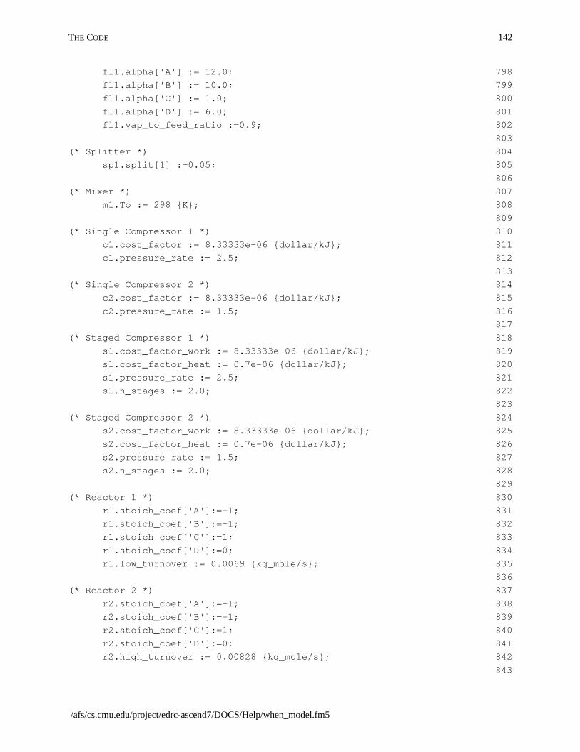
THE CODE 142
fl1.alpha['A'] := 12.0; 798
fl1.alpha['B'] := 10.0; 799
fl1.alpha['C'] := 1.0; 800
fl1.alpha['D'] := 6.0; 801
fl1.vap_to_feed_ratio :=0.9; 802
803
(* Splitter *) 804
sp1.split[1] :=0.05; 805
806
(* Mixer *) 807
m1.To := 298 {K}; 808
809
(* Single Compressor 1 *) 810
c1.cost_factor := 8.33333e-06 {dollar/kJ}; 811
c1.pressure_rate := 2.5; 812
813
(* Single Compressor 2 *) 814
c2.cost_factor := 8.33333e-06 {dollar/kJ}; 815
c2.pressure_rate := 1.5; 816
817
(* Staged Compressor 1 *) 818
s1.cost_factor_work := 8.33333e-06 {dollar/kJ}; 819
s1.cost_factor_heat := 0.7e-06 {dollar/kJ}; 820
s1.pressure_rate := 2.5; 821
s1.n_stages := 2.0; 822
823
(* Staged Compressor 2 *) 824
s2.cost_factor_work := 8.33333e-06 {dollar/kJ}; 825
s2.cost_factor_heat := 0.7e-06 {dollar/kJ}; 826
s2.pressure_rate := 1.5; 827
s2.n_stages := 2.0; 828
829
(* Reactor 1 *) 830
r1.stoich_coef['A']:=-1; 831
r1.stoich_coef['B']:=-1; 832
r1.stoich_coef['C']:=1; 833
r1.stoich_coef['D']:=0; 834
r1.low_turnover := 0.0069 {kg_mole/s}; 835
836
(* Reactor 2 *) 837
r2.stoich_coef['A']:=-1; 838
r2.stoich_coef['B']:=-1; 839
r2.stoich_coef['C']:=1; 840
r2.stoich_coef['D']:=0; 841
r2.high_turnover := 0.00828 {kg_mole/s}; 842
843
/afs/cs.cmu.edu/project/edrc-ascend7/DOCS/Help/when_model.fm5

143 A CONDITIONAL MODELING EXAMPLE: REPRESENTING A
(* Initial Guess *) 844
845
(* Flash *) 846
fl1.ave_alpha:= 5.0; 847
848
END values; 849
850
METHOD configuration2; 851
(* alternative configuration *) 852
select_feed1 := FALSE; 853
select_single1 := FALSE; 854
select_cheapr1 := FALSE; 855
select_single2 := FALSE; 856
END configuration2; 857
858
METHOD configuration3; 859
(* alternative configuration *) 860
select_feed1 := FALSE; 861
select_single1 := TRUE; 862
select_cheapr1 := TRUE; 863
select_single2 := FALSE; 864
END configuration3; 865
866
END test_flowsheet; 867
868
(* ************************************************* *) 869
870
Last modified: June 20, 1998 10:33 pm

THE PROBLEM DESCRIPTION 144
file
ple
g itD.
y
eies
into is
A.
ee B
ed,
A
CHAPTER17 A SIMPLE CHEMICAL ENGINEERING
FLOWSHEETINGEXAMPLE
In this example we shall examine a model for a simple chemicalengineering process flowsheet. The code listed below exists in thein the ASCEND examples subdirectory entitledsimple_fs.asc. Exceptfor some formatting changes to make it more presentable here, it isexactly as it is in the library version. Thus you could run this examby loading this file and using it and its corresponding scriptsimple_fs.s.
17.1 THE PROBLEM DESCRIPTION
This model is of a simple chemical engineering flowsheet. Studyinwill help to see how one constructs more complex models in ASCENModels for more complex objects are typically built out of previousldefined types each of which may itself be built of previously definedparts, etc. A flowsheet could, for example, be built of units andstreams. A distillation column could itself be built out of trays andinterconnecting streams.
Lines 40 to 56 in the code below give a diagram of the flowsheet wwould like to model. This flowsheet is to convert species B into specC. B undergoes the reaction.
B-->C
The available feed contains 5 mole percent of species A, a lightcontaminant that acts as an inert in the reactor. We pass this feed the reactor where only about 7% of B converts per pass. Species Cmuch less volatile than B which is itself somewhat less volatile thanRelative volatilities are 12, 10 and 1 respectively for A, B and C.Species A will build up if we do not let it escape from the system. Wpropose to do this by bleeding off a small portion (say 1 to 2%) of thwe recover and recycle back to the reactor.
The flowsheet contains a mixer where we mix the recycle with the fea reactor, a flash unit, and a stream splitter where we split off andremove some of the recycled species B contaminated with species
/afs/cs.cmu.edu/project/edrc-ascend7/DOCS/Help/simple_fs_model.fm5

145 A SIMPLE CHEMICAL ENGINEERINGFLOWSHEETINGEX-
e ofit to
ethis
l.
(*
s
Our goal is to determine the impact of the bleed on the performancthis flowsheet. We would also like to see if we can run the flash unget us fairly pure C as a bottom product from it.
The first type definitions we need for our simple flowsheet are for thvariables we would like to use in our model. The ones needed for example are all in the file atoms.a4l. Thus we will need to loadatoms.a4l before we load the file containing the code for this mode
The following is the code for this model. We shall interspersecomments on the code within it.
17.2 THE CODE
As the code is in our ASCEND models directory, it has headerinformation that we require of all such files included as one largecomment extending over several lines. Comments are in the form comment *).
To assure that appropriate library files are loaded first, ASCEND hathe REQUIRE statement, such as appears on line 61:
REQUIRE atoms.a4l
This statement causes the system to load the fileatoms.a4l beforecontinuing with the loading of this file.atoms.a4l in turn has a requirestatement at its beginning to causesystem.a4l to be loaded before it is.
(*********************************************************************\ 1
simple_fs.asc 2
by Arthur W. Westerberg 3
Part of the Ascend Library 4
5
This file is part of the Ascend modeling library. 6
7
Copyright (C) 1994 8
9
The Ascend modeling library is free software; you can redistribute 10
it and/or modify it under the terms of the GNU General Public License as 11
published by the Free Software Foundation; either version 2 of the 12
License, or (at your option) any later version. 13
14
The Ascend Language Interpreter is distributed in hope that it will be 15
useful, but WITHOUT ANY WARRANTY; without even the implied warranty of 16
MERCHANTABILITY or FITNESS FOR A PARTICULAR PURPOSE. See the GNU 17
Last modified: June 20, 1998 10:33 pm

THE CODE 146
General Public License for more details. 18
19
You should have received a copy of the GNU General Public License along 20
with the program; if not, write to the Free Software Foundation, Inc., 21
675 Mass Ave, Cambridge, MA 02139 USA. Check the file named COPYING. 22
23
Use of this module is demonstrated by the associated script file 24
simple_fs.s. 25
\*********************************************************************) 26
27
(*********************************************************************\ 28
$Date: 97/02/20 18:54:21 $ 29
$Revision: 1.5 $ 30
$Author: mthomas $ 31
$Source: /afs/cs.cmu.edu/project/ascend/Repository/models/examples/
simple_fs.asc,v $ 32
\*********************************************************************) 33
(* 34
35
The following example illustrates equation based modeling using the 36
ASCEND system. The process is a simple recycle process. 37
38
39
40
------- 41
| | 42
----------------------| split |----> purge 43
| | | 44
| ------- 45
| ^ 46
v | 47
----- --------- ------- 48
| | | | | | 49
----->| mix |--->| reactor |--->| flash | 50
| | | | | | 51
----- --------- ------- 52
| 53
| 54
-----> C 55
56
This model requires: “system.a4l” 57
“atoms.a4l” 58
*) 59
60
REQUIRE atoms.a4l 61
/afs/cs.cmu.edu/project/edrc-ascend7/DOCS/Help/simple_fs_model.fm5

147 A SIMPLE CHEMICAL ENGINEERINGFLOWSHEETINGEX-
es
nlyes
oandtion
Weachle
ine
The first model we shall define is for defining a stream. In thedocument entitled “Equation-based Process Modeling” we argue thneed to define a stream by maximizing the use of intensive variableand the equations interrelating them. Our problem here requires othe molar flows for the components as the problem definition providus with all the physical properties as constants. Nowhere for thissimple model do we seem to need temperatures, fugacities, etc. Tmaximize the use of intensive variables, we will use mole fractions total molar flow to characterize a stream. We must include the equathat says the mole fractions add to unity. Our first model we callmixture.
(* ************************************************* *) 62
63
MODEL mixture; 64
65
components IS_A set OF symbol_constant; 66
y[components] IS_A fraction; 67
68
SUM[y[i] | i IN components] = 1.0; 69
70
METHODS 71
METHOD clear; 72
y[components].fixed := FALSE; 73
END clear; 74
75
METHOD specify; 76
y[components].fixed := TRUE; 77
y[CHOICE[components]].fixed := FALSE; 78
END specify; 79
80
METHOD reset; 81
RUN clear; 82
RUN specify; 83
END reset; 84
85
END mixture; 86
87
Line 66 of the model for mixture defines a set of symbol constants. will later include in this set one symbol constant giving a name for eof the species in the problem (A, B and C). Line 67 defines one mofraction variable for each element in the set of components, while l69 says these mole fractions must add to 1.0.
Last modified: June 20, 1998 10:33 pm
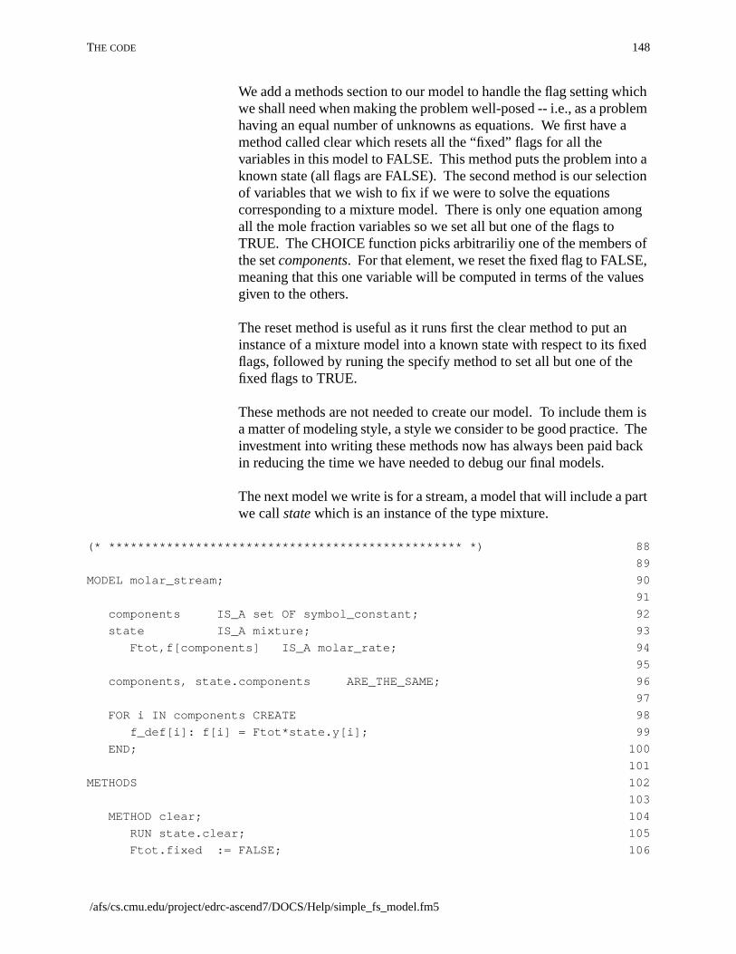
THE CODE 148
hichlem
a
o ation
ng
ofE,es
nxed
em is Theack
art
We add a methods section to our model to handle the flag setting wwe shall need when making the problem well-posed -- i.e., as a probhaving an equal number of unknowns as equations. We first have method called clear which resets all the “fixed” flags for all thevariables in this model to FALSE. This method puts the problem intknown state (all flags are FALSE). The second method is our selecof variables that we wish to fix if we were to solve the equationscorresponding to a mixture model. There is only one equation amoall the mole fraction variables so we set all but one of the flags toTRUE. The CHOICE function picks arbitrariliy one of the membersthe setcomponents. For that element, we reset the fixed flag to FALSmeaning that this one variable will be computed in terms of the valugiven to the others.
The reset method is useful as it runs first the clear method to put ainstance of a mixture model into a known state with respect to its fiflags, followed by runing the specify method to set all but one of thefixed flags to TRUE.
These methods are not needed to create our model. To include tha matter of modeling style, a style we consider to be good practice. investment into writing these methods now has always been paid bin reducing the time we have needed to debug our final models.
The next model we write is for a stream, a model that will include a pwe callstate which is an instance of the type mixture.
(* ************************************************* *) 88
89
MODEL molar_stream; 90
91
components IS_A set OF symbol_constant; 92
state IS_A mixture; 93
Ftot,f[components] IS_A molar_rate; 94
95
components, state.components ARE_THE_SAME; 96
97
FOR i IN components CREATE 98
f_def[i]: f[i] = Ftot*state.y[i]; 99
END; 100
101
METHODS 102
103
METHOD clear; 104
RUN state.clear; 105
Ftot.fixed := FALSE; 106
/afs/cs.cmu.edu/project/edrc-ascend7/DOCS/Help/simple_fs_model.fm5

149 A SIMPLE CHEMICAL ENGINEERINGFLOWSHEETINGEX-
part
, weWe
e
r theethe tod up
f[components].fixed:= FALSE; 107
END clear; 108
109
METHOD seqmod; 110
RUN state.specify; 111
state.y[components].fixed:= FALSE; 112
END seqmod; 113
114
METHOD specify; 115
RUN seqmod; 116
f[components].fixed:= TRUE; 117
END specify; 118
119
METHOD reset; 120
RUN clear; 121
RUN specify; 122
END reset; 123
124
METHOD scale; 125
FOR i IN components DO 126
f[i].nominal := f[i] + 0.1{mol/s}; 127
END; 128
Ftot.nominal := Ftot + 0.1{mol/s}; 129
END scale; 130
131
END molar_stream; 132
133
We define our stream over a set of components. We next include awhich is of type mixture and call itstate as mentioned above. We alsoinclude a variable entitledFtot which will represent the total molarflowrate for the stream. For convenience -- as they are not neededalso include the molar flows for each of the species in the stream. realize that the components defined within the part calledstate and theset of components we just defined for the stream should be the samset. We force the two sets to be the same set with theARE_THE_SAME operator.
We next write the equations that define the individual molar flows fothe components in terms of their corresponding mole fractions andtotal flowrate for the stream. Note, the equations that says the molfractions add to unity in the definition of the state forces the total of individual flowrates to equal the total flowrate. Thus we do not needinclude an equation that says the molar flowrates for the species adto the total molar flowrate for the stream.
Last modified: June 20, 1998 10:33 pm

THE CODE 150
a
od isr our ofhis
willThe of
f theet.ies the
We again write the methods we need for handling flag setting. Weleave it to the reader to establish that the specify method produceswell-posed instance involving the same number of variables to becomputed as equations available to compute them. The scale meththere as we may occasionally wish to rescale the nominal values foflows to reflect the values we are computing for them. Poor scalingvariables can lead to numerical difficulties for really large models. Tmethod is there to reduce the chance we will have poor scaling.
Note that the nominal values for the remaining variables -- the molefractions -- are unity. It does not need to be recomputed as unity isalmost always a good nominal value for each of them.
Our next model is for the first of our unit operations. Each of these be built of streams and equations that characterize their behavior. first models a mixer. It can have any number of feed streams, eachwhich is a molar stream. We require the component set for each ofeed streams and the output stream from the unit to be the same sFinally we write a component material balance for each of the specin the problem, where we sum the flows in each of the feeds to giveflow in the output stream,out.
(* ************************************************* *) 134
135
MODEL mixer; 136
137
n_inputs IS_A integer_constant; 138
feed[1..n_inputs], out IS_A molar_stream; 139
140
feed[1..n_inputs].components, 141
out.components ARE_THE_SAME; 142
143
FOR i IN out.components CREATE 144
cmb[i]: out.f[i] = SUM[feed[1..n_inputs].f[i]]; 145
END; 146
147
METHODS 148
149
METHOD clear; 150
RUN feed[1..n_inputs].clear; 151
RUN out.clear; 152
END clear; 153
154
METHOD seqmod; 155
END seqmod; 156
157
/afs/cs.cmu.edu/project/edrc-ascend7/DOCS/Help/simple_fs_model.fm5

151 A SIMPLE CHEMICAL ENGINEERINGFLOWSHEETINGEX-
tond,
oe
at,ell-g
se fory
ich
hen as willes/sone
METHOD specify; 158
RUN seqmod; 159
RUN feed[1..n_inputs].specify; 160
END specify; 161
162
METHOD reset; 163
RUN clear; 164
RUN specify; 165
END reset; 166
167
METHOD scale; 168
RUN feed[1..n_inputs].scale; 169
RUN out.scale; 170
END scale; 171
172
END mixer; 173
TheMETHOD clear sets all the fixed flags for the parts of this model false by running each of their clear methods (i.e., for all the feeds afor the stream out). If this model had introduced any new variablestheir fixed flags would have been set to FALSE here.
We will implement the method to make the model well posed into twparts:seqmod (stands for “sequential modular” which is the mindset wuse to get a unit well-posed) andspecify. The first we shall use withinany unit operation to fix exactly enough fixed flags for a unit such thif we also make the feed streams to it well-posed, the unit will be wposed. For a mixer unit, the output stream results simply from mixinthe input streams; there are no other variables to set other than thothe feeds. Thus theseqmod method is empty. It is here for consistencwith the other unit operation models we write next. TheMETHODspecify makes this model well-posed by calling theseqmod method andthen thespecify method for each of the feed streams. No other flagsneed be set to make the model well-posed.
METHOD reset simply runsclear followed byspecify. Running thissequence of method will make the problem well-posed no matter whof the fixed flags for it are set to TRUE before runningreset. Finally,flowrates can take virtually any value so we can include ascale methodto scale the flows based on their current values.
The next model is for a very simple ‘degree of conversion’ reactor. Tmodel defines a turnover rate which is the rate at which the reactiowritten proceeds (e.g., in moles/s). For example, here our reactionbe B --> C. A turnover rate of 3.7 moles/s would mean that 3.7 molof B would convert to 3.7 moles/s of C. The vector stoich_coef has
Last modified: June 20, 1998 10:33 pm

THE CODE 152
e
ets
entry per component. Here there will be three components when wtest this model so the coefficients would be 0, -1, 1 for the reaction
0 A + (-1) B + (+1) C = 0.
Reactants have a negative coefficient, products a positive one. Thmaterial balance to compute the flow out for each of the componensums the amount coming in plus that created by the reaction.
(* ************************************************* *) 174
175
MODEL reactor; 176
177
feed, out IS_A molar_stream; 178
feed.components, out.components ARE_THE_SAME; 179
180
turnover IS_A molar_rate; 181
stoich_coef[feed.components]IS_Afactor; 182
183
FOR i IN feed.components CREATE 184
out.f[i] = feed.f[i] + stoich_coef[i]*turnover; 185
END; 186
187
METHODS 188
189
METHOD clear; 190
RUN feed.clear; 191
RUN out.clear; 192
turnover.fixed := FALSE; 193
stoich_coef[feed.components].fixed := FALSE; 194
END clear; 195
196
METHOD seqmod; 197
turnover.fixed := TRUE; 198
stoich_coef[feed.components].fixed := TRUE; 199
END seqmod; 200
201
METHOD specify; 202
RUN seqmod; 203
RUN feed.specify; 204
END specify; 205
206
METHOD reset; 207
RUN clear; 208
RUN specify; 209
END reset; 210
/afs/cs.cmu.edu/project/edrc-ascend7/DOCS/Help/simple_fs_model.fm5

153 A SIMPLE CHEMICAL ENGINEERINGFLOWSHEETINGEX-
ired
tputf the
needd,
ry
211
METHOD scale; 212
RUN feed.scale; 213
RUN out.scale; 214
turnover.nominal := turnover.nominal+0.0001 {kg_mole/s}; 215
END scale; 216
217
END reactor; 218
219
TheMETHOD clear first directs all the parts of the reactor to run theclear methods. Then it sets the fixed flags for all variables introducin this model to FALSE.
Assume the feed to be known. We introduced one stoichiometriccoefficient for each component and a turnover rate. To make the oustream well-posed, we would need to compute the flows for each ocomponent flows leaving. That suggests the material balances wewrote are all needed to compute these flows. We would, therefore, to set one fixed flag to TRUE for each of the variables we introducewhich is what we do in theMETHOD seqmod. Now when we runseqmod and then thespecify method for the feed, we will have madethis model well-posed, which is what we do in theMETHOD specify.
The flash model that follows is a constant relative volatility model. Treasoning why the methods attached are as they are.
(* ************************************************* *) 220
221
MODEL flash; 222
223
feed,vap,liq IS_A molar_stream; 224
225
feed.components, 226
vap.components, 227
liq.components ARE_THE_SAME; 228
229
alpha[feed.components], 230
ave_alpha IS_A factor; 231
232
vap_to_feed_ratio IS_A fraction; 233
234
vap_to_feed_ratio*feed.Ftot = vap.Ftot; 235
236
FOR i IN feed.components CREATE 237
cmb[i]: feed.f[i] = vap.f[i] + liq.f[i]; 238
Last modified: June 20, 1998 10:33 pm

THE CODE 154
ke Thisel
eq[i]: vap.state.y[i]*ave_alpha = alpha[i]*liq.state.y[i]; 239
END; 240
241
METHODS 242
243
METHOD clear; 244
RUN feed.clear; 245
RUN vap.clear; 246
RUN liq.clear; 247
alpha[feed.components].fixed := FALSE; 248
ave_alpha.fixed := FALSE; 249
vap_to_feed_ratio.fixed := FALSE; 250
END clear; 251
252
METHOD seqmod; 253
alpha[feed.components].fixed := TRUE; 254
vap_to_feed_ratio.fixed := TRUE; 255
END seqmod; 256
257
METHOD specify; 258
RUN seqmod; 259
RUN feed.specify; 260
END specify; 261
262
METHOD reset; 263
RUN clear; 264
RUN specify; 265
END reset; 266
267
METHOD scale; 268
RUN feed.scale; 269
RUN vap.scale; 270
RUN liq.scale; 271
END scale; 272
273
END flash; 274
275
(* ************************************************* *) 276
277
The final unit operation model is the splitter. The trick here is to maall the states for all the output streams the same as that of the feed.move makes the compositions all the same and introduces only onequation to add those mole fractions to unity. The rest of the modeshould be evident.
/afs/cs.cmu.edu/project/edrc-ascend7/DOCS/Help/simple_fs_model.fm5

155 A SIMPLE CHEMICAL ENGINEERINGFLOWSHEETINGEX-
MODEL splitter; 278
279
n_outputs IS_A integer_constant; 280
feed, out[1..n_outputs ] IS_A molar_stream; 281
split[1..n_outputs] IS_A fraction; 282
283
feed.components, out[1..n_outputs].components ARE_THE_SAME; 284
285
feed.state, 286
out[1..n_outputs].state ARE_THE_SAME; 287
288
FOR j IN [1..n_outputs] CREATE 289
out[j].Ftot = split[j]*feed.Ftot; 290
END; 291
292
SUM[split[1..n_outputs]] = 1.0; 293
294
METHODS 295
296
METHOD clear; 297
RUN feed.clear; 298
RUN out[1..n_outputs].clear; 299
split[1..n_outputs-1].fixed:=FALSE; 300
END clear; 301
302
METHOD seqmod; 303
split[1..n_outputs-1].fixed:=TRUE; 304
END seqmod; 305
306
METHOD specify; 307
RUN seqmod; 308
RUN feed.specify; 309
END specify; 310
311
METHOD reset; 312
RUN clear; 313
RUN specify; 314
END reset; 315
316
METHOD scale; 317
RUN feed.scale; 318
RUN out[1..n_outputs].scale; 319
END scale; 320
321
END splitter; 322
323
Last modified: June 20, 1998 10:33 pm

THE CODE 156
asho
ng, to
duce We
tell-
ee.
(* ************************************************* *) 324
325
Now we shall see the value of writing all those methods for our unitoperations (and for the models that we used in creating them). Weconstruct our flowsheet by saying it includes a mixer, a reactor, a flunit and a splitter. The mixer will have two inputs and the splitter twoutputs. The next few statements configure our flowsheet by makifor example, the output stream from the mixer and the feed streamthe reactor be the same stream.
The methods are as simple as they look. This model does not introany variables nor any equations that are not introduced by its parts.simply ask the parts to clear their variable fixed flags.
To make the flowsheet well-posed, we ask each unit to set sufficienfixed flags to TRUE to make itself well posed were its feed stream wposed (now you can see why we wanted to create the methodsseqmodfor each of the unit types.) Then the only streams we need to makwell-posed are the feeds to the flowsheet, of which there is only onThe remaining streams come out of a unit which we can think ofcomputing the flows for it.
MODEL flowsheet; 326
327
m1 IS_A mixer; 328
r1 IS_A reactor; 329
fl1 IS_A flash; 330
sp1 IS_A splitter; 331
332
(* define sets *) 333
334
m1.n_inputs :==2; 335
sp1.n_outputs :==2; 336
337
(* wire up flowsheet *) 338
339
m1.out, r1.feed ARE_THE_SAME; 340
r1.out, fl1.feed ARE_THE_SAME; 341
fl1.vap, sp1.feed ARE_THE_SAME; 342
sp1.out[2], m1.feed[2] ARE_THE_SAME; 343
344
METHODS 345
346
METHOD clear; 347
RUN m1.clear; 348
/afs/cs.cmu.edu/project/edrc-ascend7/DOCS/Help/simple_fs_model.fm5

157 A SIMPLE CHEMICAL ENGINEERINGFLOWSHEETINGEX-
or.e an, we
.ctor
RUN r1.clear; 349
RUN fl1.clear; 350
RUN sp1.clear; 351
END clear; 352
353
METHOD seqmod; 354
RUN m1.seqmod; 355
RUN r1.seqmod; 356
RUN fl1.seqmod; 357
RUN sp1.seqmod; 358
END seqmod; 359
360
METHOD specify; 361
RUN seqmod; 362
RUN m1.feed[1].specify; 363
END specify; 364
365
METHOD reset; 366
RUN clear; 367
RUN specify; 368
END reset; 369
370
METHOD scale; 371
RUN m1.scale; 372
RUN r1.scale; 373
RUN fl1.scale; 374
RUN sp1.scale; 375
END scale; 376
377
END flowsheet; 378
379
(* ************************************************* *) 380
381
We have created a flowsheet model above. If you look at the reactmodel, we require that you specify the turnover rate for the reactionWe may have no idea of a suitable turnover rate. What we may havidea about is the conversion of species B in the reactor; for examplemay know that about 7% of the B entering the reactor may convertHow can we alter our model to allow for us to say this about the reaand not be required to specify the turnover rate? In a sequentialmodular flowsheeting system, we would use a “computationalcontroller.” We shall create a model here that gives us this samefunctionality. Thus we call it a “controller.” There are many ways toconstruct this model. We choose here to create a model that has aflowsheet as a part of it. We introduce a variable conv which will
Last modified: June 20, 1998 10:33 pm

THE CODE 158
h
ded
this
we
indicate the fraction conversion of any one of the components whicwe call the key_component here. For that component, we add amaterial balance based on the fraction of it that will convert. We adone new variable and one new equation so, if the flowsheet is well-posed, so will our controller be well-posed. However, we want tospecify the conversion rather that the turnover rate. Thespecify methodfirst asks the flowsheet fs to make itself well-posed. Then it makesone trade: fixing conv and releasing the turnover rate.
MODEL controller; 382
383
fs IS_A flowsheet; 384
conv IS_A fraction; 385
key_components IS_A symbol_constant; 386
fs.r1.out.f[key_components] = (1 - conv)*fs.r1.feed.f[key_components]; 387
388
METHODS 389
390
METHOD clear; 391
RUN fs.clear; 392
conv.fixed:=FALSE; 393
END clear; 394
395
METHOD specify; 396
RUN fs.specify; 397
fs.r1.turnover.fixed:=FALSE; 398
conv.fixed:=TRUE; 399
END specify; 400
401
METHOD reset; 402
RUN clear; 403
RUN specify; 404
END reset; 405
406
METHOD scale; 407
RUN fs.scale; 408
END scale; 409
410
END controller; 411
412
(* ************************************************* *) 413
414
We now would like to test our models to see if they work. How can write test for them? We can create test models as we do below.
/afs/cs.cmu.edu/project/edrc-ascend7/DOCS/Help/simple_fs_model.fm5

159 A SIMPLE CHEMICAL ENGINEERINGFLOWSHEETINGEX-
ouse theSo
lso
ingn
ivenandd
bles
To test the flowsheet model, we create a test_flowsheet model thatrefines our previously defined flowsheet model. “To refine the previmodel” means this model includes all the statements made to definflowsheet model plus those statements that we now provide here. this model is a flowsheet but with it components specified to be ‘A’,‘B’, and ‘C’. We add a new method calledvalues in which we specifyvalues for all the variables we intend to fix when we solve. We can aprovide values for other variables; these will be used as the initialvalues for them when we start to solve. We see all the variables begiven values with the units specified. The units must be specified iASCEND. ASCEND will interpret the lack of units to mean thevariable is unitless. If it is not, then you will get a diagnostic fromASCEND telling you that you have written a dimensionallyinconsistent relationship.
Note we specify the molar flows for the three species in the feed. Gthese flows, the equations for the stream will compute the total flow then the mole fractions for it. Thus the feed stream is fully specifiewith these flows.
We look at the seqmod method for each of the units to see the variato which we need to give values here.
MODEL test_flowsheet REFINES flowsheet; 415
416
m1.out.components:==[‘A’,’B’,’C’]; 417
418
METHODS 419
420
METHOD values; 421
m1.feed[1].f[‘A’] := 0.005 {kg_mole/s}; 422
m1.feed[1].f[‘B’] := 0.095 {kg_mole/s}; 423
m1.feed[1].f[‘C’] := 0.0 {kg_mole/s}; 424
425
r1.stoich_coef[‘A’] := 0; 426
r1.stoich_coef[‘B’] := -1; 427
r1.stoich_coef[‘C’] := 1; 428
r1.turnover := 3 {kg_mole/s}; 429
430
fl1.alpha[‘A’] := 12.0; 431
fl1.alpha[‘B’] := 10.0; 432
fl1.alpha[‘C’] := 1.0; 433
fl1.vap_to_feed_ratio := 0.9; 434
fl1.ave_alpha := 5.0; 435
436
sp1.split[1] := 0.01; 437
Last modified: June 20, 1998 10:33 pm

THE CODE 160
urel is,
an
fs Wee for
438
fl1.liq.Ftot:=m1.feed[1].f[‘B’]; 439
END values; 440
441
END test_flowsheet; 442
443
(* ************************************************* *) 444
445
Finally we would like to test our controller model. Again we write otest model as a refinement of the model to be tested. The test modtherefore, a controller itself. We make our fs model inside our testmodel into a test_flowsheet, making it a more refined type of part thit was in the controller model. We can do this because thetest_controller model is a refinement of the flowsheet model which was previously. A test_flowsheet is, as we said above, a flowsheet.create a values method which first runs the values method we wrotthe test_flowsheet model and then adds a specification for theconversion of B in the reactor.
MODEL test_controller REFINES controller; 446
447
fs IS_REFINED_TO test_flowsheet; 448
key_components :==‘B’; 449
450
METHODS 451
452
METHOD values; 453
RUN fs.values; 454
conv := 0.07; 455
END values; 456
457
END test_controller; 458
459
(* ************************************************* *) 460
461
/afs/cs.cmu.edu/project/edrc-ascend7/DOCS/Help/simple_fs_model.fm5

161 A SIMPLE CHEMICAL ENGINEERINGFLOWSHEETINGEX-
Last modified: June 20, 1998 10:33 pm

162
ionmples
n
all
ly to
y of
ns
CHAPTER18 THE ASCENDPREDEFINED
COLLECTION OF MODELS
The ASCEND system has a main directory of libraries and applicatmodels: ascend4/models. One can examine and execute these exawhen learning how to model in ASCEND.
system.a4l The file calledsystem.a4l in the libraries must always be loaded first ithe ASCEND system. It is automatically loaded when one starts theASCEND system. However, thedelete all types command will deleteall type definitions including the ones in this file. If you have deletedtypes, always reload this file first using theRead instruction in theLibrary tool set.
atoms.a4l The simplest collection of previously defined types are those whichdefine the kinds of constants, parameters and variables we are likeuse in constructing an engineering or scientific model. A file calledatoms.a4l located in the libraries subdirectory has over 125 types ofconstants, parameters and variables. Following are three of thedefinitions it contains.
CONSTANT critical_compressibility REFINES
real_constant DIMENSIONLESS; 1
2
UNIVERSAL CONSTANT speed_of_light 3
REFINES real_constant :== 1{LIGHT_C}; 4
5
ATOM volume REFINES solver_var 6
DIMENSION L^3 7
DEFAULT 100.0{ft^3}; 8
lower_bound := 0.0{ft^3}; 9
upper_bound := 1e50{ft^3}; 10
nominal := 100.0{ft^3}; 11
END volume; 12
Note that the first and third include a statement of the dimensionalitthe item being defined. For example critical compressibility isdimensionless while the dimensions for volume are L3 (i.e., lengthcubed). The ASCEND system supports nine basic dimensions asdefined for the standards defining the SI system of units. Dimensio
/afs/cs.cmu.edu/project/edrc-ascend7/DOCS/Help/library_example_files.fm5

163 THE ASCENDPREDEFINED COLLECTION OF MODELS
E),olid
ss,
g
have
ngcanlong
stleers.
differ from units in thatlength is a dimension whilefeet is a set of unitsone may use to express a length. Dimensions in ASCEND are L(length: typical units being ft, m), M (mass: kg, lbm), T (time: s, yr),(electric current: amp), Q (quantity: mole), TMP (temperature: K, RLUM (luminous intensity: candela), P (plane angle: radian) and S (sangle: steradian). We have also included the tenth dimension C(currency: USdollar) so one can express cost. If you wish to exprecost in a variety of different currencies (e.g., USdollars, UKpounds)you will have to define the conversion rates.
(See the manual entitled The ASCEND IV language syntax andsemantics for more information on dimensionality and units.)
Typical use oflibrary files
One will typically create models in the ASCEND system by includinone or more of the library files available. Almost certainly the fileatoms.a4l will become a part of any engineering or scientific model.
It would be useful for you to view this and a few of the other libraryfiles using a text editor such as xemacs to see what libraries we do available.
Examples andscripts
The examples subdirectory in ASCEND has a number of completeASCEND models. Each model is in two parts: the .a4c file containithe model definition and the .a4s file containing a script which one use to execute the model. An example is the model simple_fs.a4c awith its script simple_fs.a4s.
Each of the example files indicates which of the library files one muload and the order in which to load them before loading the exampfile. If you fail to load a library file, you will experience a large numbof diagnostic messages indicating there are missing type definition
Last modified: June 20, 1998 10:33 pm

164
mple- Ep-
, Chad
hall of theisge even item
exact
snce,
CHAPTER 19THE ASCEND IV LANGUAGE
SYNTAX AND SEMANTICS
Benjamin Allan1
Arthur W. Westerberg1
Department of Chemical Engineeringand the Engineering Design Research Center /Institute for Complex Engineered Systems
Carnegie Mellon University
1. The ASCEND language has evolved from the combined efforts of several generations of users and imentors. We wish to particularly acknowledge the contributions of ASCEND III implementors Kirk Abbott, Tomperly, Peter Piela, Boyd Safrit, Karl Westerberg, and Joe Zaher, and of the ASCEND IV crew: Duncan CoffeyFarschman, Jennifer Perry, Vicente Rico-Ramirez, Mark Thomas and Ken Tyner.
We shall present an informal description of the ASCEND IV language. Being informal, we susually include examples and descriptions of the intended semantics along with the syntaxitems. At times the inclusion of semantics will seem to anticipate later definitions. We do thbecause we would also like this chapter to be used as a reference for the ASCEND languaafter one generally understands it. Often one will need to clarify a point about a particularand will not wish to have to search in several places to do so.
Syntax is the form or structure for the statements in ASCEND, where one worries about thewords one uses, their ordering, the punctuation, etc.Semantics describe the meaning of astatement.
To distinguish between syntax and semantics, consider the statement
y IS_A fraction;
Rules on the syntax for this statement tell us we need a user supplied instance name,y, followedby the ASCEND operatorIS_A , followed by a type name (fraction). The statement terminatewith a semicolon. The statement semantics says we are declaring the existence of an insta
/afs/cs.cmu.edu/project/edrc-ascend7/DOCS/Help/syntax.fm5

165 THE ASCEND IV LANGUAGE SYNTAX AND SEMANTICS
be
ently
n under
s
shether
) in
. It is) is
ent
d
te is
ally
t
locally named y, of the type fraction as a part within the current model definition and it is toconstructed when an instance of the current model definition is constructed.
The syntax for a computer language is often defined by using a Bachus-Naur formal (BNF)description. The complete YACC and FLEX description of the language described (as presimplemented) is available by FTP2 and via the World Wide Web3. The semantics of a very highlevel modeling language such as ASCEND IV are generally much more restrictive than thesyntax. For this reason we do not include a BNF description in this paper. ASCEND IV is aexperiment. The language is under constant scrutiny and improvement, so this document isconstant revision. Contact the authors for the latest version.
19.1 PRELIMINARIES
2. In the directory ftp.cs.cmu.edu:project/ascend/gnu-ascend/ see the file README.3. http://www.cs.cmu.edu/afs/cs.cmu.edu/project/ascend/ftp/gnu-ascend/README
We will start off with some background information and some tipthat make the rest of the chapter easier to read. ASCEND is anobject-oriented (OO) language for hierarchical modeling that habeen somewhat specialized for mathematical models. Most of tspecialization is in the implementation and the user interface rathan the language definition.
We feel the single most distinguishing feature of mathematicalmodels is that solving them efficiently requires that the solvingalgorithms be able to address the entire problem eithersimultaneously or in a decomposition of the natural problemstructure that the algorithm determines is best for the machine(suse. In the ASCEND language object-orientation is used toorganize natural structures and make them easier to understandnot used to hide the details of the objects. The user (or machinefree to ignore uninteresting details, and the ASCEND environmprovides tools for the runtime suppression of these.
ASCEND is well into its 4th generation. Some features we willdescribe are not yet implemented (some merely speculative) anthese are clearly marked (* 4+ *). Any feature not marked (* 4+*)has been completely implemented, and thus any mismatchbetween the description given here and the software we distribua bug we want you to tell us about.
The syntax and semantics of ASCEND may seem at first a bitunusual. However, do not be afraid to just try what comes naturif what we write here is unclear. The parser and compiler ofASCEND IV really will help you get things right. Of course if wha
Last modified: June 20, 1998 10:32 pm
PRELIMINARIES 166
totem
s.
isis an
of
typese,
aveorents.
to
lp
d to
in
e
we write here is unclear, please ask us about it because we aimcontinuously improve both this document and the language sysit describes.
We will describe, starting in Section 19.1.2, the higher levelconcepts of ASCEND, but first some important punctuation rule
ASCEND is cAsEsensitive!
The keywords that are shown capitalized (or in lower case) in thchapter are that way because ASCEND is case sensitive. IS_A ASCEND keyword; isa, Is_a, and all the other permutations youcan think of are NOT equivalent to IS_A. In declaring new typesmodels and variables the user is free to use any style ofcapitalization he or she may prefer, however, they must remainconsistent or undefined types and instances will result.
This case restriction makes our code very readable, but hard to without a smart editor. We have kept the case-sensitivity becaulike all mathematicians, we find ourselves running out of goodvariable names if we are restricted to a 26 letter alphabet. We hdeveloped smart add-ins for two UNIX editors, EMACS and vi, fhandling the upper case keywords and some other syntax elemThe use of these editors is described in another chapter.
The ASCEND IV parser is very picky and pedantic. It also tries give helpful messages and occasionally even suggestions. Newusers should just dive in and make errors, letting the system hethem learn how to avoid errors.
19.1.1 PUNCTUATION
This section covers both the punctuation that must be understooread this document and the punctuation of ASCEND code.
keywords: ASCEND keywords and type names are given in the left columnbold format. It is generally clear from the main text which arekeywords and which are type names.
Minor items: Minor headings that are helpful in finding details are given in thleft column inunderline format.
Tips: Special notes and hints are sometimes placed on the left.
*3*: This indicates that what follows is specific to ASCEND IIIc andmay disappear in a future version of ASCEND IV. GenerallyASCEND IV will provide some equivalent functionality at 1/10thof the ASCEND III price.
/afs/cs.cmu.edu/project/edrc-ascend7/DOCS/Help/syntax.fm5

167 THE ASCEND IV LANGUAGE SYNTAX AND SEMANTICS
IIaing
ay
gh z,t it
s (.).
ers.
O
s or
}.
ce,
*4* This indicates that what follows is specific to ASCEND IVand may not be available in ASCEND IIIc. Generally ASCEND Imay provide some very klugey equivalent functionality, often at very high price in terms of increased compilation time or debuggdifficulty.
*4+* ASCEND IV functionality that is not fully implemented at the timeof this writing. The precise syntax of the final implementation mvary slightly from what is presented here. A revision of thisdocument will be made at the time of implementation.
LHS: Left Hand Side. Abbreviation used frequently.
RHS: Right Hand Side. Abbreviation used frequently.
Simple Names: In ASCEND simple names are made of the characters a throuA through Z, _, (*4+*: $). The underscore is used as a letter, bucannot be the first letter in a name. The “$” character is usedexclusively as the first character in the name of system definedbuilt-in parts. "$" is explained in more detail in Section 19.6.2.Simple names should be no more than 80 characters long.
Compound names: Compound names are simple names strung together with dotSee the description of "." below.
Groupings:
« » In documentation optional fields are surrounded by these mark
(* *) Comment. *3* Anything inside these is a comment. Comments DNOT nest in ASCEND IIIc. Comments may extend over manylines. *4* Comments DO nest in ASCEND IV.
( ) Rounded parentheses. Used to enclose arguments for functionmodels where the order of the arguments matters. Also used togroup terms in complex arithmetic, logical, or set expressionswhere the order of operations needs to be specified.
Efficiency tip: The compiler can simplify relation definitions in a particularlyefficient manner if constants are grouped together.
{ } Curly braces. Used to enclose units. For example, 1 {kg_mole/sAlso used to enclose the body of annotations.Note: Curly bracesare also used in TCL, the language of the ASCEND user interfaabout which we will say more in another chapter.
Last modified: June 20, 1998 10:32 pm

PRELIMINARIES 168
ject
esy to
red
me
thod
o.)
n
nted
[ ] Square brackets. Used to enclose sets or elements of sets.Examples: my_integer_set :== [1,2,3], demonstrates the use ofsquare brackets in the assignment of a set. My_array[1]demonstrates the use of square brackets in naming an array obindexed over an integer set which includes the element 1.
. Dot. The dot is used, as in PASCAL and C, to construct the namof nested objects. Examples: if object a has a part b, then the warefer to b is as a.b. Tray[1].vle shows a dot following a squarebracket; here Tray[1] has a part named vle.
.. Dot-dot or double dot. Integer range shorthand. For example,my_integer_set :== [1,2,3] and my_integer_set :== [1..3] areequivalent. If .. appears in a context requiring (), such as theALIASES/IS_A statement, then the range is expanded and ordeas we would naturally expect.
: Colon. A separator used in various ways, principally to set the naof an arithmetic relation apart from the definition.
:: Double colon. A separator used in the methods section foraccessing methods defined on types other than the type the meis part of. Explained in Section 19.4.
; Semicolon. The separator of statements.
19.1.2 BASIC ELEMENTS
Boolean value TRUE or FALSE. Can’t get much simpler, eh? In the languagedefinition TRUE and FALSE do not map to 1 and 0 or any othertype of numeric value. (In the implementation, of course, they d
User interface tip: The ASCEND user interface programmers have found it veryconvenient, however, to allow T/F, 1/0, Y/N, and other obviousboolean conventions as interactive input when assigning booleavalues. We are lazy users.
Integer value A signed whole number up to the maximum that can be represeby the computer on which one is running ASCEND.MAX_INTEGER is machine dependent. Examples are:
123
-5
MAX_INTEGER, typically 2147483647.
/afs/cs.cmu.edu/project/edrc-ascend7/DOCS/Help/syntax.fm5

169 THE ASCEND IV LANGUAGE SYNTAX AND SEMANTICS
issat
uter
KS
f
.
y... A
e
Real value ASCEND represents reals almost exactly as any othermathematically oriented programming language does. The manthas an optional negative sign followed by a string of digits and amost one decimal point. The exponent is the lettere or E followedby an integer. The number must not exceed the largest the compis able to handle. There can be no blank characters in a real.MAX_REAL is machine dependent. The following are legitimatereals in ASCEND:
-1
1.2
1.3e-2
7.888888e+34
.6E21
MAX_REAL, typically about 1.79E+308.
while the following are not:
1. 2 (*contains a blank within it*)
1.3e2.0 (*exponent has a decimal in it*)
+1.3 (* illegal unary + sign. x = +1.3 not allowed*)
Reals stored in SI units We store all real values as double precision numbers in the Msystem of units. This eliminates many common errors in themodeling of physical systems. Since we also place the burden oscaling equations on system routines and a simple modelingmethodology, the internal units are not of concern to most users
Dimensionality: Real values have dimensionality such as length/time for velocitDimensionality is to be distinguished from the units such as ft/sASCEND takes care of mapping between units and dimensionsvalue without units (this includes integer values) is taken to bedimensionless. Dimensionality is built up from the following basdimensions:
Name definition typical units
L length meter, m
M mass kilogram, kg
T time second, s
E electric current ampere, A
Q quantity mole, mole
Last modified: June 20, 1998 10:32 pm

PRELIMINARIES 170
of
ith
useed.
itsr
s,
t
s.roup by
otents
TMP temperature Kelvin, K
LUM luminous intensity candela, cd
P plane angle radian, rad
S solid angle steradian, srad
C currency currency, CR
The atom and constant definitions in the library illustrate the usedimensionality.
Dimensions may be any combination of these symbols along wrounded parentheses, (), and the operators *, ^ and /. ExamplesincludeM/T or M*L^2/T^2/TMP {this latter means(M*(L^2)/(T^2))/TMP }. The second operand for the “to thepower” operator, ^, must be an integer value (e.g., -2 or 3) becafractional powers of dimensional numbers are physically undefin
If the dimensionality for a real value is undefined, then ASCENDgives it a wild card dimensionality. If ASCEND can later deduce dimensionality from its use in a model definition it will do so. Foexample consider the real variablea, supposea has wild carddimensionality,b has dimensionality ofL/T. Then the statement:
Example of adimensionally consistentequation.
a + b = 3 {ft/s};
requires thata have the same dimensionality as the other two termnamely,L/T. ASCEND will assign this dimensionality toa. Theuser will be warned of dimensionally inconsistent equations.
Unit expression A unit expression may be composed of any combination of uninames defined by the system and any numerical constantscombined with times (*), divide(/) and “to the power” (^) operatorThe RHS of ^ must be an integer. Parentheses can be used to gsubexpressions EXCEPT a divide operator may not be followeda grouped subexpression.
So, {kg/m/s} is fine, but {kg/(m*s)} is not. Although the twoexpressions are mathematically equivalent, it makes the systemprogramming and output formatting easier to code and faster toexecute if we disallow expressions of the latter sort.
The units understood by the system are defined in Chapter 20. Nthat several “units” defined are really values of interesting consta
/afs/cs.cmu.edu/project/edrc-ascend7/DOCS/Help/syntax.fm5

171 THE ASCEND IV LANGUAGE SYNTAX AND SEMANTICS
.
ealst
tent
/s}
or;
a
D:
g
in SI, e.g. R :== 1{GAS_C} yields the correct value of thethermodynamic gas constant. Users can define additional units
Units A unit expression must be enclosed in curly braces {}. When a rnumber is used in a mathematical expression in ASCEND, it muhave a set of units expressed with it. If it does not, ASCENDassumes the number is dimensionless, which may not be the inof the modeler. An example is shown in the dimensionallyconsistent equation above where the number 3 has the units {ftassociated with it.
Examples:
{kg_mole/s/m} same as {(kg_mole/s)/m}
{m^3/yr}
{3/100*ft} same as {0.03*ft}
{s^-1} same as {1/s}
Illegal unit examples are
{m/(K*kg_mole)} grouped subexpression used in the denominatshould be written{m/K/kg_mole} .
{m^3.5} power of units or dimensions must be integer.
Symbol Value The format for a symbol is that of an arbitrary character stringenclosed between two single quotes. There is no way to embedsingle quote in a symbol: we are not in the escape sequencebusiness at this time. The following are legal symbols in ASCEN
’H2O'
’r1'
’Bill said,”foo” to whom?’
while the following are not legal symbol values:
"ethanol" (double quotes not allowed)
water (no single quotes given)
’i can’t do this’ (no embedded quotes)
There is an arbitrary upper limit to the number of characters in asymbol (something like 10,000) so that we may detect a missinclose quote in a bad input file without crashing.
Last modified: June 20, 1998 10:32 pm

PRELIMINARIES 172
all ofe
1, 2,ustes.ted
1) if.ents
no
the and as
of a
eak,e
her
Sets values Set values are lists of elements, all of type integer_constant or type symbol_constant, enclosed between square brackets []. Thfollowing are examples of sets:
['methane', 'ethane', 'propane']
[1..5, 7, 15]
[2..n_stages]
[1, 4, 2, 1, 16]
[]
We will say more aboutsets in 19.2.2.
The value range 1..5 is an allowable shorthand for the integers 3, 4 and 5 while the value range 2..n_stages (where n_stages mbe of type integer_constant) means all integers from 2 to n_stagIf n_stages is less than 2, then the third set is empty. The repeaoccurrence of 1 in the fourth set is ignored. The fifth set is theempty set.
We use the termset in an almost pure mathematical sense. Theelements have no order. One can only ask two things of a set: (an element is a member of it and (2) its cardinality (CARD(set))Repeated elements used in defining a set are ignored. The elemof setscannot themselves be sets in ASCEND; i.e., there can besets of set.
Sets are unordered. A set of integers may appear to be ordered to the modeler asnatural numbers have an order. However, it is the user imposingusing the ordering, not ASCEND. ASCEND sees these integerselements in the set with NO ordering. Therefore, there are nooperators in ASCEND such as successor or precursor memberset.
Arrays An array is a list of instances indexed over a set, in computer-span associative array of objects. The instances are all of the sambase type (as that is the only way they can be defined). Anindividual member of a list may later be more refined than the otmembers (we shall illustrate that possibility). The following arearrays in ASCEND.
stage[1..n_stages]
y[components]
column[areas][processes]
wherecomponents, areas andprocesses are sets. Forexamplecomponents could be the set of symbols['ethylene','propylene'], areas the set of symbols['feed_prep','prod_purification'] while
/afs/cs.cmu.edu/project/edrc-ascend7/DOCS/Help/syntax.fm5

173 THE ASCEND IV LANGUAGE SYNTAX AND SEMANTICS
ly
ut,re that
aretter
ets
processes could be the set['alcohol_manuf','poly_propropylene_manuf'] . Note that the third example(column) is a list of lists (the way that ASCEND permits a multipsubscripted array).
The following are elements in the above arrays:
stage[1]
y['ethylene']
column['feed_prep'][alcohol_manuf']
provided that n_stages is 1 or larger.
There can be any number of subscripts for an array. We point ohowever, that in virtually every application of arrays requiring mothan two subscripts, there is usually a some underlying conceptis much better modeled as an object than as part of a deeplysubscripted array. In the following jagged array example, there really the concepts of unit operation and stream that would be beunderstood if made explicit.
Arrays can be jagged (* 4 *) Arrays can be ’sparse’ or jagged. For example:
process[1..3] IS_A set OF integer;
process[1] :== [2];
process[2] :== [7,5,3];
process[3] :== [4,6];
FOR i in [1..3] CREATE
FOR j IN process[i] CREATE
flow[i][j] IS_A mass;
END FOR;
END FOR;
process is an array of sets (not to be confused with a set of swhich ASCEND does not have) andflow is an array with sixelements spread over three rows:
flow[1][2]
flow[2][7], flow[2][3], flow[2][5]
flow[3][4], flow[3][6]
Sparse arrays of models and variables are new to ASCEND IV.
Arrays are also instances Each array is itself an object. That is, when you write"a[1..2]IS_A real;" three objects get created:a[1] ,a[2] , anda. a is anarray instance which has parts named [1]
Last modified: June 20, 1998 10:32 pm

PRELIMINARIES 174
notC,
bnly
s are
dex
ent:
e
the
hssary or
is:
ment
and [2] that arereal instances. When a parameterized modelrequires an array, you pass it the single itema, not the elementsa[1..2] .
Not contiguous storage Just in case you still have not caught on, ASCEND arrays areblocks of memory such as are seen in low-level languages like FORTRAN, and Matlab. Themodeling language does not providethings like MatMult, Transpose, and Inverse because these areprocedural solving tools. If you are dedicated, you could writeMETHODs that implement matrix algebra, but this is a really dumidea. We aim to structure our software so that it can interact opewith separate, dedicated tools (such as Matlab) when those toolneeded.
Index variable One can introduce a variable as an index ranging over a set. Invariables are local to the statements in which they occur. Anexample of using an index variable is the following FOR statem
FOR i IN components CREATE
VLE_equil[i]: y[i] = K[i]*x[i];
END FOR;
In this examplei implicitly is of the same type as the values in thsetcomponents. If another objecti exists in the modelcontaining the FOR loop, it is ignored while executing thestatements in that loop. This may cause unexpected results andcompiler will generate warnings about loop index shadowedvariables.
Label: One can label statements which define arithmetic relationships(objective functions, equalities, and inequalities) in ASCEND.Labeling is highly recommended because it makes models mucmore readable and more easily debugged. Labels are also necefor relations which are going to be used in conditional modelingdifferentiation functions. A label is a sequence of alphanumericcharacters ending in a colon. An example of a labeled equation
mass_balance: m_in = m_out;
An example of a labeled objective function is:
obj1: MAXIMIZE revenue - cost;
If a relation is defined within a FOR statement, it must have anarray indexed label so that each instance created using the stateis distinguishable from the others. An example is:
/afs/cs.cmu.edu/project/edrc-ascend7/DOCS/Help/syntax.fm5
175 THE ASCEND IV LANGUAGE SYNTAX AND SEMANTICS
y
erits
e
ion.
mes
().
NDat
en the
t an
FOR i IN components CREATE
equil[i]: y[i] = K[i]*x[i];
END FOR;
The ASCEND interactive user interface identifies relationships btheir labels. If one has not provided such a label, the systemgenerates the label:
modelname_equationnumber
wheremodelname andequationnumber are the name of the modeland the equation number in the model. An example is
mixture_14
for the unlabeled 14th relation in the mixture definition. If there is aconflict caused with an existing name, the generated name hasenough letters added afterequationnumber to make it a uniquename. Remember that each model in a refinement hierarchy inhthe equations of its less refined ancestors, so the first equationappearing in the source code of a refining model may actually bthe nth relation in that model.
Lists Often in a statement one can include a list of names or expressA name list is one or more names where multiple list entries areseparated from each other by commas. Examples of a list of naare:
T1, inlet_T, outlet_T
y[components], y_in
stage[1..n_stages]
Ordered lists: If the ordering of names in a list matters, that list is enclosed inOrder matters in: calling externally defined methods or models,calling most real-valued functions, passing parameters to ASCEmodels or methods, and declaring the controlling parameters thSELECT, SWITCH, and WHEN statements make decisions on.
19.1.3 BASIC CONCEPTS
Instances and types This is an opportune time to emphasize the distinction betwetermsinstance andtype. A type in ASCEND is what we definewhen we declare an ASCEND model or atom. It is the formaldefinition of the attributes (parts) and attribute default values tha
Last modified: June 20, 1998 10:32 pm
PRELIMINARIES 176
ichive and
pe
le.
ghtn an
lt be
object will have if it is created using the type definition. Methodsare associated with types.
In ASCEND there are two meanings (closely related) of aninstance.
• An instance is anamed partthat exists within a typedefinition.
• An instance is a compiled object.
If one is in the context of the ASCEND interface, the systemcompiles an instance of a model type to create an object with whone carries out computations. The system requires the user to gsimple name for this simulation instance. This name given is thethe first part of the qualified name for all the parts of the compileobject.
Implicit types It is possible to create an instance that does not have acorresponding type definition in the library. The type of such aninstance is said to beimplicit. (Some people use the wordanonymous. However, no computable type is anonymous and theimplicit type of an instance is theoretically computable). Thesimplest example of an implicit type is the type of an instancecompiled from the built-in definitioninteger_constant . Forexample:
i, j IS_A integer_constant;
i:== 2;
j:== 3;
Instances i and j, though of the same formal type, are implicit tyincompatible because they have been assigned distinct values.
Instances which are either formally or implicitly type incompatibcannot be merged. This will be discussed further in Section 19.3
Parsing Most errors in the declaration of an ASCEND model can be cauat parse time because the object type of any well-formed name iASCEND definition can be resolved or proved ambiguous. Wecannot prove at parse time whether a specific array element wilexist, but we can know that should such an element exist, it musof the type with which the array is defined.
/afs/cs.cmu.edu/project/edrc-ascend7/DOCS/Help/syntax.fm5

177 THE ASCEND IV LANGUAGE SYNTAX AND SEMANTICS
:
rns
ot
sen
ing
ign an
re. Thents,
theOther
Ambiguity is warned about loudly because it is caused by eithermisspelling or poor modeling style. The simplest example ofambiguity follows.
Assume a type,stream , and a refinement ofstream ,heat_stream , which adds the new variable H. Now, if we write
MODEL mixer;
input[1..2] IS_A stream;
output IS_A heat_stream;
input[1].H + input[2].H = output.H;
END mixer;
We see the parser can find the definition ofH in the typeheat_stream , sooutput.H is well defined. The author of themixer model may intend to refine input[1] and input[2] to beobjects of different types, saysteam_stream andelectric_stream , where each defines anH suitable for use inthe equation. The parser cannot read the author’s mind, so it wathat input[1].H and input[2].H are ambiguous in the mixerdefinition. The mixer model is not highly reusable except by theauthor, but sometimes reusability is not a high priority objective.The mixer definition is allowed, but it may cause problems ininstantiation if the author has forgotten the assumption that is nexplicitly stated in the model and neglects to refine the inputstreams appropriately.
Instantiation Creating an simulation based on a type definition is a multi-phaprocess called compiling (or instantiation). When an instantiatiocannot be completed because some structural parameter (asymbol_constant, real_constant, boolean_constant,integer_constant, or set) does not have a value there will bePENDING statements. The user interface will warn that somethis incomplete.
In phase 1 all statements that create instance structures or assconstant values are executed. This phase theoretically requiresinfinite number of passes through the structural statements of adefinition. We allow a maximum of 5 and have never needed mothan 3. There may be pending statements at the end of phase 1compiler or interface will issue warnings about pending statemestarting with warnings about unassigned constants.
Phase 2 compiles as many real arithmetic relation definitions aspossible. Some relations may be impossible to compile becauseconstants or sets they depend on do not have values assigned.
Last modified: June 20, 1998 10:32 pm

DATA TYPE DECLARATIONS 178
hat
as the
Otheretic
s toy
e
n.
ned
ing
ele
astom
relations may be impossible because they reference variables tdo not exist. This is determined in a single pass.
Phase 3 compiles as many logical arithmetic relation definitionspossible. Some relations may be impossible to compile becauseconstants or sets they depend on do not have values assigned. relations may be impossible because they reference real arithmrelations that do not exist. This is determined in a single pass.
Phase 4 compiles as many conditional programming statement(WHENs) as possible. Some WHEN relations may be impossiblecompile because the discrete variables, models, or relations thedepend on do not exist. This is determined in a single pass.
Phase 5 executes the variable defaulting statements made in thdeclarative section of each model IF AND ONLY IF there are nopending statements from phases 1-4 anywhere in the simulatio
default_self After all phases are done, the methoddefault_self is called in thetop-most model of the simulation, if this method exists.
The first occurrence of each impossible statement will be explaiduring a failed compilation. Impossible statements include:
• Relations containing undefinable variables (oftenmisspellings).
• Assignments that are dimensionally inconsistent or containmismatched types.
• Structure building or modifying statements that refer to modparts which cannot exist or that require a type-incompatiblargument, refinement, or merge.
19.2 DATA TYPE DECLARATIONS
In the spectrum of OO languages, ASCEND is best consideredbeing class-based, though it is rather more a hybrid. We have aand model definitions, calledtypes, and the compiled objectsthemselves, calledinstances. ASCEND instances have a record ofwhat type they were constructed from.
/afs/cs.cmu.edu/project/edrc-ascend7/DOCS/Help/syntax.fm5
179 THE ASCEND IV LANGUAGE SYNTAX AND SEMANTICS
ofl
e.
n
Type qualifiers:
UNIVERSAL Universal is an optional modifier of all ATOM, CONSTANT. andMODEL definitions. If UNIVERSAL precedes the definition, thenALL instances of that type will actually refer to the first instance the type that is created. This saves memory and ensures globaconsistency of data.
Examples of universal type definitions are
UNIVERSAL MODEL methane REFINES
generic_component_model;
UNIVERSAL CONSTANT circle_constant REFINES
real_constant :== 1{PI};
UNIVERSAL ATOM counter_1 REFINES integer;
Tip: Don’t useUNIVERSAL variables inrelations.
It is important to note that, because variables must storeinformation about which relations they occur in, it is a very badidea to use UNIVERSAL typed variables in relations. Theconstruction and maintenance of the relation list becomes veryexpensive for universal variables. UNIVERSAL constants are finto use, though, because there are no relation links for constants
19.2.1 MODELS
MODEL An ASCEND model has a declarative part and an optionalprocedural part headed by the METHODS word. Models areessentially containers for variables and relations. We will explaithe various statements that can be made within models inSection 19.3 and Section 19.4.
Simple models:
foo MODEL foo;
(* statements about foo go here*)
METHODS
(* METHODs for foo go here*)
END foo;
bar MODEL bar REFINES foo;
(*additional statements about foo *)
METHODS
(* additional METHODs for bar *)
Last modified: June 20, 1998 10:32 pm

DATA TYPE DECLARATIONS 180
d and
s,ntse
ld
ys,
ne
.
END bar;
Parameterized Models (* 4 *) Parameterizing models makes them easier to understanfaster for the system to compile. The syntax for a parameterizedmodel vaguely resembles a function call in imperative languagebut it is NOT. When constructing a reusable model, all the constathat determine the sizes of arrays and other structures should bdeclared in the parameter list so that
• the user knows what is required to reuse the model.
• the compiler knows what values must be set before it shoubother attempting to compile the model.
There is no reason that other items could not also go in theparameter list, such as key variables which might be consideredinputs or outputs or control parameters in the mathematicalapplication of the model. A simple example of parameterizationwould be:
column(n,s) MODEL column(
ntrays WILL_BE integer_constant;
components IS_A set of symbol_constant;
);
stage[1..ntrays] IS_A simple_tray;
END column;
flowsheet MODEL flowsheet;
tower4size IS_A integer_constant;
tower4size :== 22;
ct IS_A column(tower4size,[’c5’,’c6’]);
(* additional flowsheet statements *)
END flowsheet;
In this example, the column model takes the first argument, ntraby reference. That is,ct.ntrays is an alias for the flowsheetinstancetower4size . tower4size must be compiled andassigned a value before we will attempt to compile the columnmodel instance ct. The second argument is taken by value,[’c5’,’c6’], and assigned tocomponents , a column partthat was declared with IS_A in the parameter list. There is only oname for this set, ct.components . Note that in the flowsheetmodel there is no part that is a set ofsymbol_constant .
The use of parameters in ASCEND modeling requires somethought, and we will present that set of thoughts in Section 19.5
/afs/cs.cmu.edu/project/edrc-ascend7/DOCS/Help/syntax.fm5

181 THE ASCEND IV LANGUAGE SYNTAX AND SEMANTICS
ntil
dase
he
, so a
thermade
ned
desthe the
h
Beginners may wish to create new models without parameters uthey are comfortable using the existing parameterized librarydefinitions. Parameters are intended to support model reuse anefficient compilation which are not issues in the very earliest phof developing novel models.
19.2.2 SETS
Arrays in ASCEND, as already discussed in Section 19.1.2, aredefined over sets. A set is simply an instance with a set value. Telements of sets are NOT instances or sets.
Set Declaration: A set is made of either symbol_constants or integer_constantsset object is declared in one of two ways:
my_integer_set IS_A set OF integer_constant;
or
my_symbol_set IS_A set OF symbol_constant;
:== A set is assigned a value like so:
my_integer_set :== [1,4];
The RHS of such an assignment must be either the name of anoset instance or an expression enclosed in square brackets and up of only set operators, other sets, and the names ofinteger_constants or symbol_constants. Sets can only be assigonce.
Set Operations
UNION[setlist] A function taken over a list of sets. The result is the set that incluall the members of all the sets in the list. Note that the result of UNION operation is an unordered set and the argument order tounion function does not matter. The syntax is:
+ UNION[list_of_sets]
A+B is shorthand forUNION[A,B]
Consider the following sets for the examples to follow.
A := [1, 2, 3, 5, 9];
B := [2, 4, 6, 8];
Then UNION[A, B] is equal to the set [1, 2, 3, 4, 5, 6, 8, 9] whicequals [1..6, 8, 9] which equals [[1..9] - [7]].
Last modified: June 20, 1998 10:32 pm
DATA TYPE DECLARATIONS 182
t lessntax
he
r of
setet
st be
do
the
odel
INTERSECTION[] INTERSECTION[list of set expressions]. Finds the intersection(and) of the sets listed.
* Equivalent to INTERSECTION[list_of_sets].
A*B is shorthand forINTERSECTION[A,B]
For the sets A and B defined just above,INTERSECTION[A, B]is the set [2] . The * shorthand for intersection is NOTrecommended for use except in libraries no one will look at.
Set difference: One can subtract one set from another. The result is the first seany members in the set union of the first and second set. The syis
- first_set - second_set
For the sets A and B defined above, the set difference A - B is tset [1, 3, 5, 9] while the set difference B - A is the set[4, 6, 8] .
CARD[set] Cardinality. Returns an integer constant value that is the numbeitems in the set.
CHOICE[set] Choose one. The result of running the CHOICE function over ais an arbitrary (but consistent: for any set instance you always gthe same result) single element of that set.
RunningCHOICE[A] gives any member from the set A. Theresult is a member, not a set. To make the result into a set, it muenclosed in square brackets. Thus[CHOICE[A]] is a set with asingle element arbitrarily chosen from the set A. Good modelersnot leave modeling decisions to the compiler; they do not useCHOICE[]. We are stuck with it for historical reasons.
To reduce a set by one element, one can use the following
A_less_one IS_A set OF integer;
A_less_one :== A - [CHOICE[A]];
IN lhs IN rhs can only be well explained by examples. IN is used inindex expressions. If lhs is a simple and not previously definedname, it is created as a temporary loop index which will take onvalues of the rhs set definition. If lhs is something that alreadyexists, the result of lhs IN rhs is a boolean value; stare at the mset_example below which demonstrates both IN andSUCH_THAT. If you still are not satisfied, you might examine[[westerbergksets]].
/afs/cs.cmu.edu/project/edrc-ascend7/DOCS/Help/syntax.fm5

183 THE ASCEND IV LANGUAGE SYNTAX AND SEMANTICS
toe
nts inet of in
orhe
SUCH_THAT (* 4 *) Set expressions can be rather clever. We will give a detailedexample from chemistry because unordered sets are unfamiliarmost people and set arithmetic is quite powerful. In this examplwe see arrays of sets and sparse arrays.
MODEL set_example;
(* we define a sparse matrix of reaction coefficient information
* and the species balance equations. *)
rxns IS_A set OF integer_constant;
rxns :== [1..3];
species IS_A set OF symbol_constant;
species :== ['A','B','C','D'];
reactants[rxns] IS_A set OF symbol_constant; (* species in each rxn_j *)
reactants[1] :== ['A','B','C'];
reactants[2] :== ['A','C'];
reactants[3] :== ['A','B','D'];
reactions[species] IS_A set OF integer_constant;
FOR i IN species CREATE (* rxns for each species i *)
reactions[i] :== [j IN rxns SUCH_THAT i IN reactants[j]];
END FOR;
(* Define sparse stoichiometric matrix. Values of eta_ij set later.*)
FOR j IN rxns CREATE
FOR i IN reactants[j] CREATE
(* eta_ij --> mole i/mole rxn j*)
eta[i][j] IS_A real_constant;
END FOR;
END FOR;
production[species] IS_A molar_rate;
rate[rxns] IS_A molar_rate; (* mole rxn j/time *)
FOR i IN species CREATE
gen_eqn[i]: production[i] =
SUM[eta[i][j]*rate[j] | j IN reactions[i]];
END FOR;
END set_example;
"|" is shorthand forSUCH_THAT.
The array eta has only 8 elements, and we defined those elemea set for each reaction. The equation needs to know about the sreactions for a species i, and that set is calculated automaticallythe model’s first FOR/CREATE statement.
| The | symbol is the ASCEND III notation for SUCH_THAT. Wenoted that "|" is often read as "for all", which is different in that "fall" makes one think of a FOR loop where the loop index is on t
Last modified: June 20, 1998 10:32 pm

DATA TYPE DECLARATIONS 184
erigned
itselfol
as
ed
onlynot
f a
. Ifs
left of an IN operator. For example, the j loop in the SUM ofgen_eqn[i] above.
19.2.3 CONSTANTS
ASCEND supports real, integer, boolean and character stringconstants. Constants in ASCEND do not have any attributes oththan their value. Constants are scalar quantities that can be assexactly once. Constants may only be assigned using the :==operator and the RHS expression they are assigned from must be constant. Constants do not have subparts. Integer and symbconstants may be used in determining the definitions of sets.
Explicit refinements of the built-in constant types may be definedexemplified in the description of real_constant. Implicit typerefinements may be done by instantiating an incompletely definconstant and assigning its final value.
Sets could be considered constant because they are assigned once, however sets are described separately because they are quite scalar quantities.
real_constant Real number with dimensionality. Note that the dimensionality oreal constant can be specified via the type definition withoutimmediately defining the value, as in the following pair ofdefinitions.
CONSTANT declarationexample:
CONSTANT molar_weight REFINES real_constant DIMENSION
M/Q;
CONSTANT hydrogen_weight REFINES molar_weight :==
1.004{g/mole};
integer_constant Integer number. Principally used in determining model structureappearing in equations, integers are evaluated as dimensionlesreals. Typical use is inside a MODEL definition and looks like:
n_trays IS_A integer_constant;
n_trays :== 50;
tray[1..n_trays] IS_A vl_equilibrium_tray;
symbol_constant Object with a symbol value. May be used in determining modelstructure.
boolean_constant Logical value. May be used in determining model structure.
/afs/cs.cmu.edu/project/edrc-ascend7/DOCS/Help/syntax.fm5
185 THE ASCEND IV LANGUAGE SYNTAX AND SEMANTICS
he
sedcts
lase
,efore
al.
is
riske
Setting constants
:== Constant and set assignment operator.
It is suggested, but notrequired, that names of alltypes that refine the built-in constant types havenames that end in_constant.
LHS_list :== RHS;
Here it is required that the one or more items in the LHS be of tsame constant type and that RHS is a single-valued expressionmade up of values, operators, and other constants. The :== is uto make clear to both the user and the system what scalar objeare constants.
19.2.4 VARIABLES
There are four built-in types which may be used to constructvariables: symbol, boolean, integer, and real. At this time symbotypes have special restrictions. Refinements of these variable btypes are defined with the ATOM statement. Atom types maydeclare attribute fields with types real, integer, boolean, symboland set. These attributes are NOT independent objects and thercannot be refined, merged, or put in a refinement clique(ARE_ALIKEd).
ATOM The syntax for declaring a new atom type is
ATOM atom_type_name REFINES variable_type
«DIMENSION dimension_expression»
«DEFAULT value»; (* note the ; *)
«initial attribute assignment;»
END atom_type_name;
DEFAULT,DIMENSION, andDIMENSIONLESS
The DIMENSION attribute is for variables whose base type is reIt is an optional field. If not defined for any atom with base typereal, the dimensions will be left as undefined. Any variable whichlater declared to be one of these types will be givenwild carddimensionality (represented in the interactive display by an aste(*)). The system will deduce the dimensionality from its use in threlationships in which it appears or in the declaring of defaultvalues for it, if possible.
solver_var is a specialcase of ATOM and wewill say much moreabout it in Section 19.6.1.
ATOM solver_var REFINES real DEFAULT 0.5 {?};
lower_bound IS_A real;
upper_bound IS_A real;
nominal IS_A real;
fixed IS_A boolean;
Last modified: June 20, 1998 10:32 pm

DATA TYPE DECLARATIONS 186
ich
nit
e be
the
nt
gslly
rs
eentg
latere
fixed := FALSE;
lower_bound := -1e20 {?};
upper_bound := 1e20 {?};
nominal := 0.5 {?};
END solver_var;
The default field is also optional. If the atom has a declareddimensionality, then this value must be expressed with units whare compatible with this dimensionality. In thesolver_varexample, we see a DEFAULT value of 0.5 with the unspecified u{?} which leaves the dimensionality wild.
real Real valued variable quantity. At present, all variables that youwant to be attended to by solver tools must be refinements of thtype solver_var. This is so that modifiable parametric values canincluded in equations without treating them as variables. Strictlyspeaking, this is a characteristic of the solver interface and not ASCEND language. Each tool in the total ASCEND system mayhave its own semantics that go beyond the ASCEND objectdefinition language.
integer Integer valued variable quantity. We find these mighty conveniefor use in certain procedural computations and as attributes ofsolver_var atoms.
boolean Truth valued variable quantity. These are principally used as flaon solver_vars and relations. They can also be used proceduraand as variables in logical programming models, subject to thelogical solver tool’s semantics. (Comparesolver_boolean andboolean_var in Section 19.6.)
symbol *4* Symbol valued variable quantity. We do not yet have operatofor building symbols out of other symbols.
Setting variables
:= Procedural equals differs from the ordinary equals (=) in that itmeans the left-hand-side (LHS) variables are to be assigned thvalue of the right-hand-side (RHS) expression when this statemis processed. Processing happens in the last phase of compilin(INSTANTIATION on page 177) or when executing a methodinteractively through the ASCEND user interface. The order thesystem encounters these statements matters, therefore, with a result overwriting an earlier one if both statements have the samthe same LHS variable.
/afs/cs.cmu.edu/project/edrc-ascend7/DOCS/Help/syntax.fm5

187 THE ASCEND IV LANGUAGE SYNTAX AND SEMANTICS
e ofT
ation at
are
isnts
f a
Note that variable assignments (also known as “defaultingstatements”) written in the declarative section are executed onlyafter an instance has been fully created. This is a frequent sourcconfusion and errors, therefore we recommend that you DO NOASSIGN VARIABLES IN THE DECLARATIVE SECTION.
Note that := IS NOT =. We use an ordinary equals (=) when defining a real valued equto state that the LHS expression is to equal the RHS expressionthe solution for the model. We use == for logical equations.
Tabular assignments (* 4+ *) Assigning values en masse to arrays of variables thatdefined associatively on sets without order presents a minorchallenge. The solution proposed in ASCEND IV (but not yetimplemented as we’ve not had time or significant user demand)to allow a tabular data statement to be used to assign the elemeof arrays of variables or constants. The DATA statement may beused to assign variables in the declarative or methods section omodel (though we discourage its use declaratively for variableinitialization) or to assign constant arrays of any type, includingsets, in the declarative section. Here are some examples:
DATA (* 4+ *) MODEL tabular_ex;
lset,rset,cset IS_A set OF integer_constant;
rset :== [1..3];
cset :== rset - [2];
lset :== [5,7];
a[rset][cset] IS_A real;
b[lset][cset][rset] IS_A real_constant;
(* rectangle table *)
DATA FOR a:
COLUMNS 1,3; (*order last subscript cset*)
UNITS {kg/s}, {s}; (* columnar units *)
(* give leading subscripts *)
[1] 2.8, 0.3;
[2] 2.7, 1.3;
[3] 3.3, 0.6;
END DATA;
(* 2 layer rectangle table *)
CONSTANT DATA FOR b:
COLUMNS 1..3; (* order last subscript rset *)
(* UNITS omitted, so either the user gives value in the
table or values given are DIMENSIONLESS. *)
(* ordering over [lset][cset] required *)
[5][1] 3 {m}, 2{m}, 1{m};
Last modified: June 20, 1998 10:32 pm

DATA TYPE DECLARATIONS 188
s
tionn.
lity.
e of
n a
areopsts.
[5][3] 0.1, 0.2, 0.3;
[7][1] -3 {m/s}, -2{m/s}, -1{m/s};
[7][3] 4.1 {1/s}, 4.2 {1/s}, 4.3 {1/s};
END DATA;
END tabular_ex;
For sparse arrays of variables or constants, the COLUMNS and(possibly) UNITS keywords are omitted and the array subscriptare simply enumerated along with the values to be assigned.
19.2.5 RELATIONS
Mathematical expression: The syntax for a mathematical expression is any legal combinaof variable names and arithmetic operators in the normal notatioAn expression may contain any number of matched roundedparentheses, (), to clarify meaning. The following is a legalarithmetic expression:
y^2+(sin(x)-tan(z))*q
Each additive term in a mathematical expression (terms areseparated by + or - operators) must have the same dimensiona
An expression may contain an index variable as a part of thecalculation if that index variable is over a set whose elements artype integer. (See the FOR/CREATE and FOR/DO statementsbelow.) An example is:
term[i] = a[i]*x^(i-1);
Numerical relations The syntax for a numeric relation is either
optional_label: LHS relational_operator RHS;
or
optional_label: objective_type LHS;
Objective_type is eitherMAXIMIZE orMINIMIZE . RHS andLHS must be one or more variables, constants, and operators inormal algebraic expression. The operators allowed are definedbelow and in Section 19.6.3. Variable integers, booleans, andsymbols are not allowed as operands in numerical relations, norboolean constants. Integer indices declared in FOR/CREATE loare allowed in relations, and they are treated as integer constan
/afs/cs.cmu.edu/project/edrc-ascend7/DOCS/Help/syntax.fm5

189 THE ASCEND IV LANGUAGE SYNTAX AND SEMANTICS
.
r
d
rt
ic
Relational operators:
=, >=, <=, <, >,<>
These are the numerical relational operators for declarative use
Ftot*y['methane'] = m['methane'];
y['ethanol'] >= 0;
Equations must be dimensionally correct.
MAXIMIZE,MINIMIZE
Objective function indicators.
Binary Operators: +, -, *, /, ^. We follow the usual algebraic order of operations fobinary operators.
+ Plus. Numerical addition or set union.
- Minus. Numerical subtraction or set difference.
* Times. Numerical multiplication or set intersection.
/ Divide. Numeric division. In most cases it implies real division annot integer division.
^ Power. Numeric exponentiation. If the value of y in x^y is notinteger, then x must be greater than 0.0 and dimensionless.
Unary Operators: -,ordered_function()
- Unary minus. Numeric negation. There is no unary + operator.
ordered_function ()
unary real valued functions. The unary real functions we suppoare given in section Section 19.6.3.
Real functions of sets ofreal terms:
SUM[term set] Add all expressions in the function’s list.
For the SUM, the base type real items can be arbitrary arithmetexpressions. The resulting items must all be dimensionallycompatible.
An examples of the use is:
Last modified: June 20, 1998 10:32 pm

DATA TYPE DECLARATIONS 190
a
ple:
n
n
euseng to
nce
SUM[y[components]] = 1;
or, equivalently, one could write:
SUM[y[i] | i IN components] = 1;
Empty SUM[] yieldswild 0.
When a SUM is compiled over a list which is empty it generateswild dimensioned 0. This will sometimes cause our dimensionchecking routines to fail. The best way to prevent this is to makesure the SUM never actually encounters an empty list. For exam
SUM[Q[possibly_empty_set], 0{watt}];
In the above, the variablesQ[i] (if they exist) have thedimensionality associated with an energy rate. When the set isempty, the 0 is the only term in the SUM and establishes thedimensionality of the result. When the set is NOT empty thecompiler will simplify away thetrailing 0 in the sum.
PROD[term set] Multiply all the expressions in the product’s list. The product of aempty list is a dimensionless value, 1.0.
Possible future functions: (Not implemented - only under confused consideration at thistime.) The following functions only work in methods as they arenot smooth function and would destroy a Newton-based solutioalgorithm if used in defining a model equation:
MAX[term set] (* 4+ *) maximum value on list of arguments
MIN[term set] (* 4+ *) minimum value on list of arguments
19.2.6 DERIVATIVES IN RELATIONS (* 4+ *)
Simply put, we would like to have general partial and fullderivatives usable in writing equations, as there are manymathematically interesting things that can be said about both. Whave not implemented such things yet for lack of time and becawith several implementations (see gPROMS and OMOLA, amoothers) already out there we can’t see too many research pointsbe gained by more derivative work.
19.2.7 EXTERNAL RELATIONS
We cannot document these at the present time. The only referefor them is [[abbottthesis]].
/afs/cs.cmu.edu/project/edrc-ascend7/DOCS/Help/syntax.fm5
191 THE ASCEND IV LANGUAGE SYNTAX AND SEMANTICS
be used
f
es
1
ce
r on
19.2.8 CONDITIONAL RELATIONS (* 4 *)
The syntax is CONDITIONAL list_of_relation_statements ENDCONDITIONAL;
A CONDITIONAL statement can appear anywhere in thedeclarative portion of the model and it contains only relations toused as boundaries. That is, these real arithmetic equations arein expressing logical condition equations via the SATISFIEDoperator. See LOGICAL FUNCTIONS on page 215.
19.2.9 LOGICAL RELATIONS (* 4 *)
Logical expression An expression whose value is TRUE or FALSE is a logicalexpression. Such expressions may contain boolean variables. IA,B , andlaminar areboolean , then the following is a logicalexpression:
A + (B * laminar)
as is (and probably more clearly)
A OR (B AND laminar)
The plus operator acts like an OR among the terms while the timoperator acts like an AND. Think of TRUE being equal to 1 andFALSE being equal to 0 with the 1+1=0+1=1+0=1, 0+0=0, 1*1=and 0*1=1*0=0*0=0. IfA = FALSE, B=TRUE andlaminar isTRUE, this expression has the value
FALSE OR (TRUE AND TRUE) -->TRUE
or in terms of ones and zeros
0 + (1 * 1) --> 1.
Logical relations are then made by putting together logicalexpressions with the boolean relational operators == and !=. Sinwe have no logical solving engine we have not pushed theimplementation of logical relations very hard yet.
19.2.10 NOTES (* 4 *)
Within a MODEL(or METHOD) definition annotations (hereaftercalled notes) may be made on a part declared in the MODEL, o
Last modified: June 20, 1998 10:32 pm

DATA TYPE DECLARATIONS 192
n
e of
ed
the
at aitsameonly
ksall
the MODEL (or METHOD) itself. Short notes may be made whedefining or refining an object by enclosing the note in "doublequotes." Longer notes may be made in a block statement.
Each note is entered in a database with the name of the file, namMODEL, name of METHOD if applicable, and the language (akind of keyword) in which the note is written. Users, userinterfaces, and other programs may query this database forinformation on models and simulations. The block notes mayinclude code fragments in other languages that you wish to embin your MODEL or any other kind of text.
Short notes should be included as you write any model to clarifyroles of parts and variables. All short notes have the language'inline.' Here are some examples of short notes:
L[1..10] "L[i] is the length of the ith rod"
IS_A distance;
thetaM "angle between horizon and moon",
thetaJ "angle between horizon and jupiter"
IS_A angle;
car.tires "using car in Minnesota, you betcha"
IS_REFINED_TO snow_tire;
In the second IS_A statement concerning two angles, we see thshort note in double quotes goes with the name immediately to left. We also see that the note comes before the comma if the nis part of a list of names. In the third statement, we see that not simple names but also qualified names may be annotated.
Longer notes are made in block statements of the form below.These blocks can appear in a METHOD or MODEL. These bloccan also be written separately before or after a model as we shsee.
NOTES
'language or keyword' list.of, names {
free-form block of text to store in the database
exactly as written.
}
some.other.name {
this note has the same language or keyword as the
first since we didn't define a new keyword in single
quotes before the name list.
}
'another language' some.other.name {
/afs/cs.cmu.edu/project/edrc-ascend7/DOCS/Help/syntax.fm5

193 THE ASCEND IV LANGUAGE SYNTAX AND SEMANTICS
e of
ke
d
ation
the
en espanol
}
'fortran' SELF {
This model should be solved with subroutine LSODE.
This note demonstrates that "SELF" can be used to
annotate the entire model instead of a named part.
}
END NOTES;
Notes made outside the scope of a model definition look like onthe following:
ADD NOTES IN name_of_model;
'language or keyword' list.of, names {
more text
} (* more than one note may be made in this block if
desired. *)
END NOTES;
ADD NOTES IN name_of_model METHOD name_of_method;
'language or keyword' SELF {
This method proves Fermat's last theorem and makes
toast.
}
'humor' SELF {
ASCEND is not expected to make either proving FLT or
toasting possible.
}
END NOTES;
We can add notes to the database before or after defining theannotated model. This is handy for several reasons including:
• Lengthy notes mixed with model and method code can mathat code very hard to read.
• Separate notes describing a family of models can be loadeand browsed before loading that library family.
• Users other than the author of a model can annotate thatmodel without fear of introducing typographical errors intothe model.
These advantages come with a disadvantage that all documenthas. If you change the model, you ought to change thedocumentation at the same time. To make finding thesedocumentation locations in need of change easier, the name offile containing each note is included in the loaded database.
Last modified: June 20, 1998 10:32 pm

DECLARATIVE STATEMENTS 194
ctly
and
veThef an
of
entss inle
s a partS/
tsH
,
on
C
e
Experience has shown that even documentation embedded direin models or in other computer programs gets out-dated if theperson changing the program is in a hurry and is not required todocument properly as part of the task at hand. Neither ASCENDnor any other software system can eliminate the garbage code documentation that results from undisciplined modeling.
19.3 DECLARATIVE STATEMENTS
We have already seen several examples that included declaratistatements. Here we will be more systematic in defining things. statements we describe are legal within the declarative portion oATOM or MODEL definition. The declarative portion stops at thekeyword METHODS if it is present in the definition or at the end the definition.
Statements Statements in ASCEND terminate with a semicolon (;). Statemmay extend over any number of lines. They may have blank linethe middle of them. There may be several statements on a singline.
Compound statements Some statements in ASCEND can contain other statements aof them. The declarative compound statements are the ALIASEIS_A, CONDITIONAL, FOR/CREATE, SELECT/CASE, andWHEN/CASE statements. The procedural compound statemenallowed only in methods are the FOR/DO, FOR/CHECK, SWITC(* 4 *) and the IF statements. Compound statements end with "ENDword ; ", whereword matches the beginning of the syntax blocke.g.END FOR.and they can be nested, with some exceptionswhich are noted later.
CASE statements arehere, finally!
(*4*) WHEN/CASE, CONDITIONAL, and SELECT/CASEhandle modeling alternatives within a single definition. The easyway to remember the difference is that the first picks whichequations to solve WHEN discretevariables have certain values,while the second SELECTs which statements to compile baseddiscreteconstants. (* 4 *) SWITCH statements handle flow ofcontrol in methods, in a slightly more generalized form than thelanguage switch statement.
Type declarations are notcompound statements.
MODEL and ATOM type definitions and METHOD definitions arnot really compound statements because they require a namefollowing their END word that matches the name given at thebeginning of the definition. These definitions cannot be nested.
/afs/cs.cmu.edu/project/edrc-ascend7/DOCS/Help/syntax.fm5

195 THE ASCEND IV LANGUAGE SYNTAX AND SEMANTICS
nd
ach
iled
to
isan
he
annt of
ese of
en
ues
of
ASCEND operatorsynopses:
We’ll start with an extremely brief synopsis of what each does athen give detailed descriptions. It is helpful to remember that aninstance may have many names, even in the same scope, but ename may only be defined once.
IS_A Constructor. Calls for one or more named instances to be compusing the type specified. (* 4 *) If the type is one that requiresparameters, the parameters must be supplied in () following thetype name.
IS_REFINED_TO Reconstructor. Causes the already compiled instance(s) namedhave their type changed to a more refined type. This causes anincremental recompilation of the instance(s). IS_REFINED_TO not a redefinition of the named instances because refinement conly add compatible information. The instances retain all thestructure that originally defined them. (* 4 *) If the type beingrefined to requires arguments, these must be supplied, even if tsame arguments were required in the IS_A of the originally lessrefined declaration of the instance.
ALIASES (* 4 *) Part alternate naming statement. Establishes another name forinstance at the same scope or in a child instance. The equivalean ALIASES in ASCEND III is to create another part with thedesired name and merge it immediately via ARE_THE_SAMEwith the part being renamed, a rather expensive and unintuitiveprocess.
ALIASES/IS_A(*4*)
Creates an array of alternate names for a list of existing instancwith some common base type and creates the set over which thelements of the array are indexed. Useful for making collectionsrelated objects in ways the original author of the model didn’tanticipate. Also useful for assembling array arguments toparameterized type definitions.
WILL_BE (* 4 *) Forward declaration statement. Promises that a part with the givtype will be constructed by an as yet unknown IS_A statementabove the current scope. At present WILL_BE is legal only indefining parameters. Were it legal in the body of a model,compiling models would be very expensive.
ARE_THE_SAME Merge. Calls for two or more instances already compiled to bemerged recursively. This essentially means combining all the valin the instances into the most refined of the instances and thendestroying all the extra, possibly less refined, instances. Theremaining instance has its original name and also all the namesthe instances destroyed during the merge.
Last modified: June 20, 1998 10:32 pm

DECLARATIVE STATEMENTS 196
ione
edinctsented.
tset
s a
nts.
e
ns
orreses
WILL_BE_THE_SAME(* 4 *)
Structural condition statement restricting objects in a forwarddeclaration. The objects passed to a parameterized type definitcan be constrained to have arbitrary parts in common before thparameterized object is constructed.
WILL_NOT_BE_THE_SAME (* 4 *)
Structural condition statement restricting objects in a forwarddeclaration. We apologize for the length of this key word, but webet it is easy to remember. The objects passed to a parameteriztype definition can be constrained to have arbitrary parts be distinstances before the parameterized object is constructed. At prethe constraint is only enforced when the objects are being pass
ARE_NOT_THE_SAME(* 4+ *)
Cannot be merged. We believe it is useful to say that two objeccannot be merged and still represent a valid model. This is not yimplemented, however, mainly for lack of time. Theimplementation is simple.
ARE_ALIKE Refinement clique constructor. Causes a group of instances toalways be of the same formal type. Refining one of them causerefinement of all the others. Does not propagateimplicit typeinformation, such as assignments to constants or part refinememade from a scope other than the scope of the formal definition
FOR/CREATE Indexed execution of other declarative statements. Required forcreating arrays of relations and sparse arrays of other types.
FOR/CHECK Indexed checking of the conditions (WHERE statements) of aparameterized model.
SELECT/CASE (*4*) Select a subset of statements to compile. Given the values of thspecifiedconstants, SELECT compiles all cases that match thosevalues. A name cannot be defined two different ways inside theSELECT statement, but it may be defined outside the casestatement and thenrefined in different ways in separate cases.
CONDITIONAL (*4*) Describe bounding relations. The relations written inside aCONDITIONAL statement must all be labelled. These relationscan be used to define regions in which alternate sets of equatioapply using the WHEN statement.
WHEN/CASE (* 4 *) When logicalvariables have certain values, use certain relations model parts in defining a mathematical problem. The relations anot defined inside the WHEN statement because all the relationmust be compiled regardless of which values the logical variablhave at any given moment.
/afs/cs.cmu.edu/project/edrc-ascend7/DOCS/Help/syntax.fm5
197 THE ASCEND IV LANGUAGE SYNTAX AND SEMANTICS
rds
plieds
eof
ddou
, if
tione
of
on
esh
lled
Reminder: In the following detailed statement descriptions, we show keywoin capital letters. These words must appear in capital letters asshown in ASCEND statements. We show optional parts to astatement enclosed in double angle brackets (« ») and user supnames in lower-caseitalic letters. (Remember that ASCEND treatthe underscore (_) as a letter). The user may substitute any namdesired for these names. We use names that describe the kind name the user should use.
Operators in detail:
IS_A This statement has the syntax
list_of_instance_names IS_Amodel_name«(arguments_if_needed)»;
The IS_A statement allows us to declareinstances of a giventype toexist within a model definition. Iftype has not been defined (loadein the ASCEND environment) then this statement is an error anthe MODEL it appears in is irreparably damaged (at least until ydelete the type definitions and reload a corrected file). Similarlythe arguments needed are not supplied or if provably incorrectarguments are supplied, the statement is in error. The construcof the instances does not occur until all the arguments satisfy thdefinition oftype.
If a name is used twice in WILL_BE/IS_A/ALIASES statements the same model, ASCEND will complain bitterly when thedefinition is parsed. Duplicate naming is a serious error. Labelsrelations share the same name space as other objects.
IS_REFINED_TO This statement has the syntax
list_of_instances IS_REFINED_TO
type_name «(arguments_if_needed)»;
We use this statement to change the type of each of the instanclisted to the typetype_name. The modeler has to have defined eacmember on the list of instances. Thetype_name has to be a typewhich refines the types of all the instances on the list.
An example of its use is as follows. First we define the parts cafl1, fl2 and fl3 which are of type flash.
fl1, fl2, fl3 IS_A flash;
Last modified: June 20, 1998 10:32 pm

DECLARATIVE STATEMENTS 198
onsan
pe
any
he
Se, e.g.
ceES
h
of bned
: if
Assume that there exists in the previously defined model definitithe type adiabatic_flash that is a refinement of flash. Then we cmake fl1 and fl3 into more refined types by stating:
fl1, fl3 IS_REFINED_TO adiabatic_flash;
This reconstruction does not occur until the arguments to the tysatisfy the definitiontype_name.
ALIASES (* 4 *) This statement has the syntax
list_of_instances ALIASES instance_name ;
We use this statement to point at an already existing instance oftype other thanrelation , logical_relation , orwhen. Forexample, say we want a flash tank model to have a variable T, ttemperature of the vapor-liquid equilibrium mixture in the tank.
MODEL tank;
feed, liquid, vapor IS_A stream;
state IS_A VLE_mixture;
T ALIASES state.T;
liquor_temperature ALIASES T;
END tank;
We might also want a more descriptive name than T, so ALIASEcan also be used to establish a second name at the same scopliquor_temperature .
An ALIASES statement will not be executed until the RHS instanhas been created with an IS_A. The compiler schedules ALIASinstructions appropriately and issues warnings if recursion isdetected. An array of aliases, e.g.
b[1..n], c ALIASES a;
is permitted (though we can’t think why anyone would want sucan array), and the sets over which the array is defined must becompleted before the statement is executed. So, in the exampleand c, the array b will not be created until a exists and n is assiga value. b and c will be created at the same time since they aredefined in the same statement. This suggests the following ruleyou must use an array of aliases, do not declare it in the samestatement with a scalar alias.
/afs/cs.cmu.edu/project/edrc-ascend7/DOCS/Help/syntax.fm5
199 THE ASCEND IV LANGUAGE SYNTAX AND SEMANTICS
aybe
ce is
gh
and
es
e list
not
is
The ALIASES RHS can be an element or portion of a larger arrwith the following exception. The existing RHS instance cannot a relation or array of relations (including logical relations andwhens) because of the rule in the language that a relation instanassociated with exactly one model.
ALIASES/IS_A(*4*)
The ALIASES/IS_A statement syntax is subject to change, thousome equivalent will always exist. We take a set ofsymbol_constant or integer_constant and pair it with alist of instances to create an array. For the moment, the syntax semantics is as follows.
alias_array_instance[aset] ALIASES(list_of_instances ) WHEREaset IS_A set OFsettype ;
or
alias_array_instance[aset] ALIASES(list_of_instances ) WHEREaset IS_A set OFsettypeWITH_VALUE ( value_list_matching_settype );
aset is the name of the set that will be created by the IS_A toindex the array of aliases. Ifvalue_list_matching_set_type is not given, thecompiler will make one up out of the integers (1..number of namin list_of_instances ) or symbols derived from theindividual names given. If the value list is given, it must have thesame number of elements as the list of instances does. The valuelements must be unique because they form a set. The list ofinstances can contain duplicates. If any of these conditions are met properly, the statement is in error.
ALIASES/IS_A can be used inside a FOR statement. When thisoccurs, the definition ofaset must be indexed and it must be thelast subscript ofalias_array_instance . The statement mustlook like:
array_instance[FOR_index][aset[FORindex]]ALIASES (list_of_instances ) WHEREaset[FORindex] IS_A set OFsettype WITH_VALUE( value_list_matching_settype );
Here, as with the unindexed version, the WITH_VALUE portion optional.
Last modified: June 20, 1998 10:32 pm

DECLARATIVE STATEMENTS 200
ent,nat
tlled
r
of
e
as
oft
e in
If this explanation is unclear, just try it out. The compiler errormessages for ALIASES/IS_A are particularly good because weknow it is a bit tricky to explain.
WILL_BE (* 4 *) instance WILL_BE type_name ;
The most common use of this forward declaration is as a statemwithin the parameter list of a model definition. In parameter listslist_of_instances must contain exactly one instance. Whea model definition includes a parameter defined by WILL_BE, thmodel cannot be compiled until a compiled instance at least asrefined as the type specified bytype_name is passed to it.
(* 4+ *) The second potential use of WILL_BE is to establish thaan array of a common base type exists and its elements will be fiin individually by IS_A or ARE_THE_SAME or ALIASESstatements. WILL_BE allows us to avoid costly reconstruction omerge operations by establishing a placeholder instance whichcontains just enough type information to let us check the validityother statements that require type compatibility while delayingconstruction until it is called for by the filling in statements.Instances declared with WILL_BE are never compiled if they arnot ultimately resolved to another instance created with IS_A.Unresolved WILL_BE instances will appear in the user interfaceobjects of type PENDING_INSTANCE_model_name. Because ofthe many implementation and explanation difficulties this usageWILL_BE creates, it is not allowed. The ALIASES/IS_A construcdoes the same job in a much simpler way.
ARE_THE_SAME The format for this instruction is
list_of_instancesARE_THE_SAME;
All items on the list must have compatible types. For the examplFig. 1, consider a model where we define the following parts:
a1 IS_A A;
b1 IS_A B;
c1 IS_A C;
d1 IS_A D;
e1 IS_A E;
Then the following ARE_THE_SAME statement is legal
a1, b1, c1 ARE_THE_SAME;
/afs/cs.cmu.edu/project/edrc-ascend7/DOCS/Help/syntax.fm5

201 THE ASCEND IV LANGUAGE SYNTAX AND SEMANTICS
.”
e
alltype
fo byc.,
while the following are not
b1, d1 ARE_THE_SAME;
a1, c1, d1 ARE_THE_SAME;
b1, e1 ARE_THE_SAME;
When compiling a model, ASCEND will put all of the instancesmentioned as being the same into an ARE_THE_SAME “cliqueASCEND lists members of this clique when one asks via theinterface for the aliases of any object in a compiled model.
Merging any other item with a member of the clique makes it thsame as all the other items in the clique, i.e., it adds the newlymentioned items to the existing clique.
ASCEND merges all members of a clique by first checking that members of the clique are type compatible. It then changes the designation of all clique members to that of the most refinedmember.
Figure 1. Diagram of the model type hierarchy A,B,C,D,E
It next looks inside each of the instances, all of which are now othe same type, and puts all of the parts with the same name inttheir respective ARE_THE_SAME cliques. The process repeatsprocessing these cliques until all parts of all parts of all parts, et
A
C
D
E
B
refines refines
refines
Last modified: June 20, 1998 10:32 pm

DECLARATIVE STATEMENTS 202
gr a
aIf a
nednts
andin by
tialch
f
are their respective most refined type or discovered to be typeincompatible.
There are now lots of cliques associated with the instances beinmerged. The type associated with each such clique is now eithemodel, an array, or an atom (i.e., a variable, constant, or set). Ifmodel, only one member of the clique generates its equations. variable, it assigns all members to the same storage location.
Note that the values of constants and sets are essentiallytypeinformation, so merging two already assigned constants is onlypossible if merging them does not force one of them to be assiga new value. Merging arrays with mismatching ranges of elemeis an error.
WILL_BE_THE_SAME(* 4 *)
There is no further explanation of WILL_BE_THE_SAME.
WILL_NOT_BE_THE_SAME (* 4 *)
There is no further explanation of WILL_NOT_BE_THE_SAME.
ARE_NOT_THE_SAME(* 4+ *)
ARE_NOT_THE_SAME will be documented further when it isimplemented.
ARE_ALIKE The format for this statement is
list_of_instance_names ARE_ALIKE;
The compiler places all instances in the list into an ARE_ALIKEclique. It checks that the members are formally type compatible then it converts each into the most refined type of any instance the clique. At that point the compiler stops. It does not continueplacing the parts into cliques nor does it merge anything.
There are important consequences of modeling with such a parmerge. The consequences we are about to describe can be mumore reliably achieved by use of parameterized types,when thetypes are well understood. When we are exploring new ways ofmodeling, ARE_ALIKE still has its uses. When a model and itsinitial uses are understood well enough to be put into a reusablelibrary, then parameterization and the explicit statement ofstructural constraints by operators such asWILL_NOT_BE_THE_SAME should be the preferred method oensuring correct use.
/afs/cs.cmu.edu/project/edrc-ascend7/DOCS/Help/syntax.fm5

203 THE ASCEND IV LANGUAGE SYNTAX AND SEMANTICS
elertice
r or
ams
t
to
nt ofal
sn
E in
ofoes
of
ksat
One consequence of ARE_ALIKE is to prevent extreme modelmisuse when configuring models. For example, suppose a modcreates a new pressure changing model. The modeler is not yeconcerned about the type of the streams into and out of the devbut does care that these streams are of the same final type. Foexample, the modeler wants both to be liquid streams if either isboth to be vapor streams if either is. By declaring both to be streonly but declaring the two streams to be alike, the modeleraccomplishes this intent. Suppose the modeler merges the inlestream with a liquid outlet stream from a reactor. The mergeoperation makes the inlet stream into a liquid stream. The outlestream, being in an ARE_ALIKE clique with the inlet stream, alsbecomes a liquid stream. Any subsequent merge of the outletstream with a vapor stream will lead to an error due to typeincompatibility when ASCEND attempts to compile that merge.Without the ARE_ALIKE statement, the compiler can detect nosuch incompatibility unless parameterized models are used.
Another purpose is the propagation of types through a model.Altering the type of the inlet stream through merging it with aliquid stream automatically made the outlet stream into a liquidstream.
If all the liquid streams within a distillation column are alike, thethe modeler can make them all into streams with a particular secomponents in them and with the same method used for physicproperty evaluation by merging only one of them with a liquidstream of this type. This isthe primary example which has beenused to justify the existence of ARE_ALIKE. We have observedthat its use makes a column library very difficult to compileefficiently. But since we now have parameterized types to help ukeep the column library semantically consistent, ARE_ALIKE cabe left to its proper role: the rapid prototyping of partiallyunderstood models. We have yet to see anyone use ARE_ALIKa prototyping context, however.
Finally, because ARE_ALIKE does not recursively put the partsARE_ALIKEd instances into ARE_ALIKE cliques, it is possible tARE_ALIKE model instances which have compatible formal typbut incompatibleimplicit types. This can lead to unexpectedproblems later and makes the ARE_ALIKE instruction a sourcenon-reusability.
FOR/CREATE The FOR/CREATE statement is a compound statement that loolike a loop. It isn’t, however, necessarily compiled as a loop. WhFOR really does is specify an index set value. Its format is:
Last modified: June 20, 1998 10:32 pm

PROCEDURAL STATEMENTS 204
tionnce the
d in
are
r
ary
ified
mnt
FOR index_variable IN set CREATE
list_of_statements;
END FOR;
This statement can be in the declarative part of the model definionly. Every statement in the list should have at least one occurreof the index variable, or the statement should be moved outsideFOR to avoid redundant execution. A correct example is
FOR i IN components CREATE
a.y[i], b[i] ARE_THE_SAME;
y[i] = K[i]*x[i];
END FOR;
FOR loops can be nested to produce sparse arrays as illustrateARRAYS CAN BE JAGGED on page 173. IS_A and ALIASESstatements are allowed in FOR loops, provided the statements properly indexed, a new feature in ASCEND IV.
SELECT/CASE (*4*) Declarative. Order does not matter. All matching cases areexecuted. The OTHERWISE is executed if present and no otheCASEs match. SELECT is not allowed inside FOR. Writing FORstatements inside SELECT is allowed.
CONDITIONAL (*4*) Both real and logical relations are allowed in CONDITIONALstatements. CONDITIONAL is really just a shorthand for settingthe $boundary flag on a whole batch of relations, since $boundis a write-once attribute invisible through the user interface andmethods at this time.
WHEN/CASE (* 4 *) Inside each CASE, relations or model parts to be used are specby writing, for example, USE mass_balance_1;. The method ofdealing with the combined logical/nonlinear model is left to thesolver. All matching CASEs are included in the problem to besolved.
19.4 PROCEDURAL STATEMENTS
METHODS This statement separates the method definitions in ASCEND frothe declarative statements. All statements following this statemeare to define methods in ASCEND while all before it are for thedeclarative part of ASCEND. The syntax for this statement issimply
METHODS
/afs/cs.cmu.edu/project/edrc-ascend7/DOCS/Help/syntax.fm5

205 THE ASCEND IV LANGUAGE SYNTAX AND SEMANTICS
s,
fteringethod
eadye
d.
adyes
ee oftedas
ely,
with no punctuation. The next code must be a METHOD or theEND of the type being defined. If there are no method definitionthis statement may be omitted.
METHOD definitions for a type can also be added or replaced athe type has been defined. This is to make creating and debuggof methods as interactive as possible. In ASCEND III an instancmust be destroyed and recreated each time a new or revised meis added to the type definition. This is a very expensive processwhen working with models of significant size.
The detailed semantics of method inheritance, addition, andreplacement of methods are given at the end of this section.
ADD METHODS INtype_name; (*4*)
This statement allows new methods to be added to an alreadyloaded type definition. The next code must be a METHOD or thEND METHODS; statement. If a method of the same name alreexists intype_name , the statement is in error. If other types refintype_name then the addition follows the method inheritancerules. Any type which inherited methods fromtype_name nowinherits the methods added totype_name . If a refinement oftype_name already defines a method ADDed totype_name ,then the existing method in the more refined type is not disturbe
REPLACE METHODSIN type_name;(*4*)
This statement allows existing methods to be replaced in an alreloaded type definition. The next code must be a METHOD or thEND METHODS; statement. If a method of the same name doenot exist intype_name , the statement is in error. If other typesrefinetype_name then the replacement follows the methodinheritance rules. Any type which inherited the old method nowinherits the replacment method instead.
ADD METHODS INDEFINITION MODEL;
This statement allows methods to be added globally. It should bused very sparingly. Library basemodel.a4l contains the examplthis statement. Methods in the global model definition are inheriby all models. There is no actual global model definition, but it ha method list for practical purposes.
Initialization routines:
METHOD A method in ASCEND must appear following the METHODSstatement within a model. The system executes proceduralstatements of the method in the order they are written.
At present, there are no local variables or other structures inmethods except loop indices. A method may be written recursiv
Last modified: June 20, 1998 10:32 pm

PROCEDURAL STATEMENTS 206
the
texted, and ahe
t to
it
but there is an arbitrary stack depth limit (currently set to 20 incompiler/initialize.h) to prevent the system from crashing oninfinite recursions.
Specifically disallowed in ASCEND III methods are IS_A,ALIASES, WILL_BE, IS, IS_REFINED_TO, ARE_THE_SAMEand ARE_ALIKE statements as these “declare” the structure of model and belong only in the declarative section.
(* 4+ *) In the near future, declarations of local instances (whichare automatically destroyed when the method exits) will beallowed. Since methods are imperative, these local structuredefinitions are processed in the order they are written. Localstructures are not allowed to shadow structures in the model conwith which the method is called. When local structures are allowit will also be possible to define methods which take parametersreturn values, thereby making the imperative ASCEND methodsrapid prototyping tool every bit as powerful and easy to use as tdeclarative ASCEND language.
The syntax for a method declaration is
METHOD method_name;
«procedural statement;» (*one or more*)
END method_name;
Procedural assignment The syntax is
instance_name := mathematical_expression;
or
array_name[set_name] := expression;
or
list_of_instance_names := expression.
Its meaning is that the value for the variable(s) on the LHS is sethe value of the expression on the RHS.
DATA statements (DATA (* 4+ *) on page 187) can (should,rather) also appear in methods.
FOR/DO statement This statement is similar to the FOR/CREATE statement exceptcan only appear in a method definition. An example would be
FOR i IN [1..n_stages] DO
T[i] := T[1] + (i-1)*DT;
...
/afs/cs.cmu.edu/project/edrc-ascend7/DOCS/Help/syntax.fm5

207 THE ASCEND IV LANGUAGE SYNTAX AND SEMANTICS
tax
,asear
t
at
of
END FOR;
Here we actually execute using the values of iin the sequencegiven.So,
FOR i IN [n_stages..1] DO ... END FOR;
is an empty loop, while
FOR i IN [n_stages..1] DECREASING DO ... END FOR;
is a backward loop.
IF The IF statement can only appear in a method definition. Its synis
IF logical_expression THEN
list_of_statements
ELSE
list_of_statements
END IF;
or
IF logical_expression THEN
list_of_statements
END IF;
If the logical expression has a value of TRUE, ASCEND willexecute the statements in the THEN part. If the value is FALSEASCEND executes the statements in the optional ELSE part. Pleuse () to make the precedence of AND, OR, NOT, ==, and != cleto both the user and the system.
SWITCH (* 4 *) Essentially roughly equivalent to the C switch statement, excepthat ASCEND allows wildcard matches, allows any number ofcontrolling variables to be given in a list, and assumes BREAK the end of each CASE.
CALL External calls are not presently well defined, pending debuggingthe EXTERNAL connection prototype originally created by KirkAbbott.
RUN This statement can appear only in a method. Its format is:
RUN name_of_method ;
Last modified: June 20, 1998 10:32 pm

PARAMETERIZED MODELS 208
tned the
theed
.
l beodel
or
RUN part_name.name_of_method ;
or
RUN model_type :: name_of_method ;
The named method can be defined in the current model (the firssyntax), or in any of its parts (the second syntax). Methods defiin a part will be run in the scope of that part, not at the scope ofRUN statement.
Type access to methods: Whenmodel_type:: appears, the type named must be a type that current model is refined from. In this way, methods may be definincrementally. For example:
MODEL foo;
x IS_A generic_real;
METHODS
METHOD specify;
x.fixed:= TRUE;
END specify;
END foo;
MODEL bar REFINES foo;
y IS_A generic_real;
METHODS
METHOD specify;
RUN foo::specify;
y.fixed := TRUE;
END specify;
END bar;
19.5 PARAMETERIZED MODELS
Parameterized model definitions have the following general form
MODEL new_type(parameter_list;)
«WHERE (where_list;)»
«REFINES existing_type «(assignment_list;)»»;
19.5.1 THE PARAMETER LIST
A parameter list is a list of statements about the objects that wilpassed into the model being defined when an instance of that mis created by IS_A or IS_REFINED_TO. The parameter list is
/afs/cs.cmu.edu/project/edrc-ascend7/DOCS/Help/syntax.fm5

209 THE ASCEND IV LANGUAGE SYNTAX AND SEMANTICS
puteeks
es
,s
e
e
ave
eate
kpy
nts
f
nt,mal
designed to allow a complete statement of the necessary andsufficient conditions to construct the parameterized model. Themechanism implemented is general, however, so it is possible toless than the necessary information in the parameter list if one sto confuse the model’s reusers. To make parameters easy tounderstand for users with experience in other computer languag(and to make the implementation much simpler), we define theparameter list as ordered. All the statements in a parameter listincluding the last one, must end with a ";". A parameter list looklike:
MODEL test (
x WILL_BE real;
n IS_A integer_constant;
p[1..n] IS_A integer_constant;
q[0..2*n-1] WILL_BE widget;
);
Each WILL_BE statement corresponds to a single object that thuser must create and pass into the definition oftest . We willestablish the local namex for the first object passed to thedefinition oftest . n is handled similarly, and it must preceed thdefinition ofp[1..n] , because it defines the set for the arrayp.Constant types can also be defined with WILL_BE, though we hused IS_A for the exampletest .
Each IS_A statement corresponds to a single constant-valuedinstance or an array of constant-valued instances that we will cras part of the model we are defining. Thus, the user oftest mustsupply an array of constants as the third argument. We will checthat the instance supplied is subscripted on the set [1..n] and cothe corresponding values to the array p we create local to theinstance oftest .
WILL_BE statements can be used to pass complex objects(models) or arrays of objects. Both WILL_BE and IS_A statemecan be passed arguments that aremore refined than the type listed.If an object that isless refined than the type listed, the instance oparameterized modeltest will not be compiled. When aparameterized model type is specified with a WILL_BE statemeNO arguments should be given. We are only interested in the fortype of the argument, not how it was constructed.
Last modified: June 20, 1998 10:32 pm

PARAMETERIZED MODELS 210
nts ats a
ized
is
e
teren
ngft
entanyypes,
of afore
ese
19.5.2 THE WHERE LIST
We can write structural and equation constraints on the argumein the WHERE list. Each statement is a WILL_BE_THE_SAME,WILL_NOT_BE_THE_SAME, an equation written in terms of seor discrete constants, or a FOR/CHECK statement surroundinggroup of such statements. Until all the conditions in the WHERElist are satisfied, an object cannot be constructed using theparameterized definition. If the arguments given to a parametertype in an IS_A or IS_REFINED_TO statement cannot possiblysatisfy the conditions, the IS_A or IS_REFINED_TO statement abandoned by the compiler.
We have not created a WILL_BE_ALIKE statement becauseformal type compatibility in ASCEND is not really a meaningfulguarantee of object compatibility. Object compatibility is muchmore reliably guaranteed by checking conditions on the structurdetermining constants of a model instance.
19.5.3 THE ASSIGNMENT LIST
When we declare constant parameters with IS_A, we can in a larefinement of the parameterized model assign their values in thassignment list, thus removing them from the parameter list. If aarray of constants is declared with IS_A, then we must assignvalues to ALL the array elements at the same time if we are goito remove them from the parameter list. If an array element is leout, the type which assigns some of the elements and anysubsequent refinements of that type will not be compilable.
19.5.4 REFINING PARAMETERIZED TYPES
Because we wish to make the parameterized model lists represall the parameters and conditions necessary to use a model of type, we must repeat the parameters declared in the ancestral twhen we make a refinement. If we did not repeat the parameterthe user would be forced to hunt up the (possibly long) chain oftypes that yield an interesting definition in order to know the listparameters and conditions that must be satisfied in order to usemodel. We repeat all the parameters of the type being refined bewe add new ones. The only exception to this is that parametersdefined with IS_A and then assigned in theassignment_listare not repeated because the user no longer needs to supply thvalues. A refinement of the modeltest given in Section 19.5.1follows.
/afs/cs.cmu.edu/project/edrc-ascend7/DOCS/Help/syntax.fm5

211 THE ASCEND IV LANGUAGE SYNTAX AND SEMANTICS
sat all
o
at
ng
MODEL expanded_test (
x WILL_BE real;
p[1..n] IS_A integer_constant;
q[0..2*n-1] WILL_BE better_widget;
r[0..q[0].k] WILL_BE gizmo;
ms WILL_BE set OF symbol_constant;
) WHERE (
q[0].k >= 2;
r[0..q[0].k].giz_part WILL_BE_THE_SAME;
) REFINES test(
n :== 4;
);
In expanded_test , we see that the type of the arrayq is morerefined than it was intest . We see that constants and sets frominside passed objects, such asq[0].k , can be used to set the sizeof subseqent array arguments. We see a structural constraint ththegizmo s in the arrayr must have been constructed with thesamegiz_part . This condition probably indicates that the gizmdefinition takesgiz_part as a WILL_BE defined parameter.
19.6 MISCELLANY
19.6.1 VARIABLES FOR SOLVERS
solver_var Solver_var is the base-type for allcomputable variables in thecurrent ASCEND system. Any instances of an atom definition threfines solver_var are considered potential variables whenconstructing a problem for one of the solvers.
Solver_var has wild card dimensionality. (Wild card means thatuntil ASCEND can decide what its dimensionality is, it has noneassigned. ASCEND can decide on dimensionality while compilior executing.) In system.a4l we define the following parts withassociated initial values for each:
Attributes: type default
lower_bound real 0.0
upper_bound real 0.0
nominal real 0.0
Last modified: June 20, 1998 10:32 pm

MISCELLANY 212
ee
bleasdt
ich
emi-erles.
that
s
4l
er
ses
ad
fixed boolean FALSE
lower_boundandupper_bound are bounds for a variable which armonitored and maintained during solving. The nominal value thvalue used to scale a variable when solving. The flagfixed indicatesif the variable is to be held fixed during solving. All atoms whichare refinements of solver_var will have these parts. The refiningdefinitions may reassign the default values of the attributes.
The latest full definition of solver_var is always in the filesystem.a4l.
generic_real One should not declare a variable to be of type solver_var. Thenominal value and bound values will get you into trouble whensolving. If you are programming and do not wish to declare variatypes, then declare them to be of type generic_real. This type hnominal value of 0.5 and lower and upper bounds of -1.0e50 an1.0e50 respectively. It is dimensionless. Generic_real is the firsrefinement of solver_var and is also defined in system.a4l.
Kluges for MILPs Also defined in system.a4l are the types for integer, binary, andsemi-continuous variables.
solver_semi,solver_integer,solver_binary
We define basic refinements of solver_var to support solvers whare more than simply algebraic. Various mixed integer-linearprogram solvers can be fed solver_semi based atoms defining scontinuous variables, solver_integer based atoms defining integvariables, and solver_binary based atoms defining binary variab
Integers are relaxable. All these types have associated boolean flags which indicateeither the variable is to be treated according to its restrictedmeaning or it is to be relaxed and treated as a normal continuoualgebraic variable.
Kluges for ODEs We have an alternate version of system.a4l called ivpsystem.awhich adds extra flags to the definition of solver_var in order tosupport initial value problem (IVP) solvers (integrators).Integration in the ASCEND IV environment is explained in anothchapter.
ivpsystem.a4l Having ivpsystem.a4l is a temporary, but highly effective, way tokeep people who want to use ASCEND only for algebraic purpofrom having to pay for the IVP overhead. Algebraic users loadsystem.a4l. Users who want both algebraic and IVP capability loivpsystem.a4l instead of system.a4l. This method is temporarybecause part of the extended definition of ASCEND IV is that
/afs/cs.cmu.edu/project/edrc-ascend7/DOCS/Help/syntax.fm5
213 THE ASCEND IV LANGUAGE SYNTAX AND SEMANTICS
atesing
ute the
iredent
differential calculus constructs will be explicitly supported by thecompiler. The calculus is not yet implemented, however.
19.6.2 SUPPORTED ATTRIBUTES
(* 4+ *) The solver_var, and in fact most objects in ASCEND IV, shouldhave built-in support for (and thereby efficient storage of) quite few more attributes than are defined above. These built-in attribuare not instances of any sort, merely values. The syntax for namone of these supported attributes is:object_name.$ supported_attribute_name.
Supported attributes may have symbol, real, integer, or booleanvalues. Note that the$ syntax is essentially the same as thederivative syntax for relations; derivatives are a supported attribof relations. The supported attributes must be defined at the timeASCEND compiler is built. The storage requirement for asupported boolean attribute is 1 bit rather than the 24 bytes requto store a run-time defined boolean flag. Similarly, the requiremfor a supported real attribute is 4 or 8 bytes instead of 24 bytes.
19.6.3 SINGLE OPERAND REAL FUNCTIONS :
exp() exponential (i.e., exp(x) = ex)
ln() log to the base e
sin() sine. argument must be an angle.
cos() cosine. argument must be an angle.
tan() tangent. argument must be an angle.
arcsin() inverse sine. return value is an angle.
arccos() inverse cosine. return value is an angle.
arctan() inverse tangent. return value is an angle.
erf() error function (not available from Microsoft Windoze)
sinh() hyperbolic sine
cosh() hyperbolic cosine
Last modified: June 20, 1998 10:32 pm

MISCELLANY 214
as
lueme
, P.
ed
nest
tanh() hyperbolic tangent
arcsinh() inverse hyperbolic sine
arccosh() inverse hyperbolic cosine
arctanh() inverse hyperbolic tangent
lnm() modified ln function. This lnm function is parameterized by aconstant a, which is typically set to about 1.e-8. lnm(x) is definedfollows:
ln(x) for x > a
(x-a)/a + ln(a) for x <= a.
Below the value a (default setting is 1.0e-8), lnm takes on the vagiven by the straight line passing through ln(a) and having the saslope as ln(a) has at a. This function and its first derivative arecontinuous. The second derivative contains a jump at a.
The lnm function can tolerate a negative argument while the lnfunction cannot. At present the value of a is controllable via theuser interface of the ASCEND solvers.
Operand dimensionalitymust be correct.
The operands for an ASCEND function must be dimensionallyconsistent with the function in question. Most transcendentalfunctions require dimensionless arguments. The trigonometricfunctions require arguments with dimensionality of plane anglesASCEND functions return dimensionally correct results.
The operands for ASCEND functions are enclosed within roundparentheses, (). An example of use is:
y = A*exp(-B/T);
Discontinuous functions: Discontinuous functions may destroy a Newton-based solutioalgorithm if used in defining a model equation. We strongly suggconsidering alternative formulations of your equations.
abs() absolute value of argument. Any dimensionality is allowed in anabs() function.
/afs/cs.cmu.edu/project/edrc-ascend7/DOCS/Help/syntax.fm5

215 THE ASCEND IV LANGUAGE SYNTAX AND SEMANTICS
niven.otr
asic
20
ITSntil
r
or
ust
rateses
19.6.4 LOGICAL FUNCTIONS
SATISFIED() (*4*) SATISFIED(relation_name,tolerance) returns TRUE if the relationamed has a residual value less than the real value, tolerance, gIf the relation named is a logical relation, the tolerance should nbe specified, since logical relations evaluate directly to TRUE oFALSE.
19.6.5 UNITSDEFINITIONS
As noted in 19.1.2, ASCEND will recognize conversion factorswhen it sees them as {units). These units are built up from the bunits, and new units can be defined by the user. Note that theassignment x:= 0.5 {100}; yields x == 50, and that there are no'offset conversions,' e.g. F=9/5C+32. Please keep unit names tocharacters or less as this makes life pretty for other users
One or more unit conversion factors can be defined with the UNkeyword. A unit of measure, once defined, stays in the system uthe system is shut down. A measuring unit cannot be defineddifferently without first shutting down the system, but duplicate oequivalent definitions are quietly ignored.
A UNITS declaration can occur in a file by itself, inside a model inside an atom. UNITS definitions are parsed immediately, theywill be processed even if a surrounding MODEL or ATOMdefinition is rejected. Because units and dimensionality aredesigned into the deepest levels of the system, a unit definition mbe parsed before any atoms or relations use that definition. It isgood design practice to keep customized unit definitions in sepafiles and REQUIRE those files at the beginning of any file that uthem. Unit definitions are made in the form, for example:
UNITS (* several unit definitions could be here. *)
ohm = {kilogram*meter^2/second^3/ampere^2};
END UNITS;
The standard units library, measures.a4l, is documented inChapter 20.
Last modified: June 20, 1998 10:32 pm

MISCELLANY 216
/afs/cs.cmu.edu/project/edrc-ascend7/DOCS/Help/syntax.fm5

217 THE ASCEND IV LANGUAGE SYNTAX AND SEMANTICS
Last modified: June 20, 1998 10:32 pm

tve.
D
. Weve
ll
ion
CHAPTER20 UNITS LIBRARY
20.1 UNITS
This chapter defines the dimensions and units and all the attendanconversion factors. Note that all conversions are simply multiplicatiThis information is from the file models/measures.a4l in the ASCENsource code.
Note that units can be easily defined to suit the needs of local usersare always on the lookout for new and interesting units, so if you hasome send them in. From measures.a4l we have:
20.2 THE BASIC UNITS IN AN EXTENDED SI MKSSYSTEM
These units (kilogram, mole, et c.) are associated with thedimensionality listed here (M, Q, et c.) by the ASCEND IV C code. Aother units are derived from these by multiplication factors. Use ofunits other than these requires loading unit definitions, either frommeasures.a4l or from another ASCEND file containing a UNITSdeclaration. The system rejects loudly any model or variable definitusing undefined units.
define kilogram M; (* internal mass unit SI *)
define mole Q; (* internal quantity unit SI *)
define second T; (* internal time unit SI *)
define meter L; (* internal length unit SI *)
define Kelvin TMP; (* internal temperature unit SI *)
define currency C; (* internal currency unit *)
define ampere E; (* internal electric current unit SI suggested *)
219 UNITS LIBRARY
define candela LUM; (* internal luminous intensity unit SI *)
define radian P; (* internal plane angle unit SI suggested *)
define steradian S; (* internal solid angle unit SI suggested *)
20.3 UNITS DEFINED IN MEASURES .A4L, THE
DEFAULT SYSTEM UNITS LIBRARY OF
ATOMS.A4L.
distance pc = 3.08374e+16*meter;
parsec = pc;
kpc = 1000*pc;
Mpc = 1e6*pc;
km = meter*1000;
m = meter;
dm = meter/10;
cm = meter/100;
mm = meter/1000;
um = meter/1000000;
nm = 1.e-9*meter;
kilometer = km;
centimeter = cm;
millimeter = mm;
micron=um;
nanometer = nm;
angstrom = m/1e10;
fermi = m/1e15;
Last modified: June 20, 1998 10:33 pm

UNITS DEFINED IN MEASURES.A4L, THE DEFAULT SYSTEM UNITS LIBRARY OF ATOMS.A4L. 220
mi = 1609.344*meter;
yd = 0.914412*meter;
ft = 0.304804*meter;
inch = 0.0254*meter;
mile = mi;
yard = yd;
feet = ft;
foot = ft;
in = inch;
mass metton = kilogram *1000;
mton = kilogram *1000;
kg = kilogram;
g = kilogram/1000;
gram = g;
mg = g/1000;
milligram = mg;
ug= kilogram*1e-9;
microgram = ug;
ng=kilogram*1e-12;
nanogram=ng;
pg=kilogram*1e-15;
picogram=pg;
amu = 1.661e-27*kilogram;
/afs/cs.cmu.edu/project/edrc-ascend7/DOCS/Help/measures.fm5
221 UNITS LIBRARY
lbm = 4.535924e-1*kilogram;
ton = lbm*2000;
oz = 0.028349525*kilogram;
slug = 14.5939*kilogram;
time yr = 31557600*second;
wk = 604800*second;
dy = 86400*second;
hr = 3600*second;
min = 60*second;
sec = second;
s = second;
ms = second/1000;
us = second/1e6;
ns = second/1e9;
ps = second/1e12;
year = yr;
week = wk;
day = dy;
hour = hr;
minute = min;
millisecond = ms;
microsecond = us;
nanosecond = ns;
Last modified: June 20, 1998 10:33 pm

UNITS DEFINED IN MEASURES.A4L, THE DEFAULT SYSTEM UNITS LIBRARY OF ATOMS.A4L. 222
picosecond = ps;
molecular quantities kg_mole=1000*mole;
g_mole = mole;
gm_mole = mole;
kmol = 1000*mole;
mol = mole;
mmol = mole/1000;
millimole=mmol;
umol = mole/1e6;
micromole=umol;
lb_mole = 4.535924e+2*mole;
temperature K = Kelvin;
R = 5*Kelvin/9;
Rankine = R;
money dollar = currency;
US = currency;
USdollar=currency;
CR = currency;
credits=currency;
reciprocal time(frequency)
rev = 1.0;
cycle = rev;
rpm = rev/minute;
rps = rev/second;
/afs/cs.cmu.edu/project/edrc-ascend7/DOCS/Help/measures.fm5

223 UNITS LIBRARY
hertz = cycle/second;
Hz = hertz;
area ha = meter^2*10000;
hectare=ha;
acre= meter^2*4046.856;
volume l = meter^3/1000;
liter = l;
ml = liter/1000;
ul = liter/1e6;
milliliter = ml;
microliter = ul;
hogshead=2.384809e-1*meter^3;
cuft = 0.02831698*meter^3;
impgal = 4.52837e-3*meter^3;
gal = 3.785412e-3*meter^3;
barrel = 42.0*gal;
gallon = gal;
quart = gal/4;
pint = gal/8;
cup = gal/16;
floz = gal/128;
force N = kilogram*meter/second^2;
newton = N;
Last modified: June 20, 1998 10:33 pm

UNITS DEFINED IN MEASURES.A4L, THE DEFAULT SYSTEM UNITS LIBRARY OF ATOMS.A4L. 224
dyne = N*1.0e-5;
pn=N*1e-9;
picoNewton=pn;
lbf = N*4.448221;
pressure Pa = kilogram/meter/second^2;
MPa = 1.0e+6*Pa;
bar =1.0e+5*Pa;
kPa = 1000*Pa;
pascal = Pa;
atm = Pa*101325.0;
mmHg = 133.322*Pa;
torr = 133.322*Pa;
psia = 6894.733*Pa;
psi = psia;
ftH2O = 2989*Pa;
energy J = kilogram*meter^2/second^2;
joule = J;
MJ = J * 1000000;
kJ = J * 1000;
mJ=J*1.0e-3;
uJ=J*1.0e-6;
nJ=J*1.0e-9;
milliJoule=mJ;
/afs/cs.cmu.edu/project/edrc-ascend7/DOCS/Help/measures.fm5

225 UNITS LIBRARY
microJoule=uJ;
nanoJoule=nJ;
erg = J*1.0e-7;
BTU = 1055.056*J;
pCu = BTU * 1.8;
cal = J*4.18393;
calorie = cal;
kcal=1000*calorie;
Cal=1000*calorie;
power W = J/second;
EW = 1.0e+18*W;
PW = 1.0e+15*W;
TW = 1.0e+12*W;
GW = 1.0e+9*W;
MW = 1.0e+6*W;
kW = 1000*W;
mW = W/1000;
uW = W/1000000;
nW = W/1e9;
pW = W/1e12;
fW = W/1e15;
aW = W/1e18;
terawatt = TW;
Last modified: June 20, 1998 10:33 pm

UNITS DEFINED IN MEASURES.A4L, THE DEFAULT SYSTEM UNITS LIBRARY OF ATOMS.A4L. 226
gigawatt = GW;
megawatt = MW;
kilowatt = kW;
watt = W;
milliwatt = mW;
microwatt = uW;
nanowatt = nW;
picowatt = pW;
femtowatt = fW;
attowatt = aW;
hp= 7.456998e+2*W;
absolute viscosity poise = Pa*s;
cP = poise/100;
electric charge coulomb=ampere*second;
C = coulomb;
coul = coulomb;
mC = 0.001*C;
uC = 1e-6*C;
nC = 1e-9*C;
pC = 1e-12*C;
miscellaneous electro-magnetic fun
V = kilogram*meter^2/second^3/ampere;
F = ampere^2*second^4/kilogram/meter^2;
ohm = kilogram*meter^2/second^3/ampere^2;
/afs/cs.cmu.edu/project/edrc-ascend7/DOCS/Help/measures.fm5

227 UNITS LIBRARY
mho = ampere^2*second^3/kilogram/meter^2;
S = mho;
siemens = S;
A=ampere;
amp = ampere;
volt = V;
farad= F;
mA= A/1000;
uA= A/1000000;
kV= 1000*V;
MV= 1e6*V;
mV= V/1000;
mF = 0.001*F;
uF = 1e-6*F;
nF = 1e-9*F;
pF = 1e-12*F;
kohm = 1000*ohm;
Mohm = 1e6*ohm;
kS = 1000*S;
mS = 0.001*S;
uS = 1e-6*S;
Wb = V*second;
weber = Wb;
Last modified: June 20, 1998 10:33 pm

UNITS DEFINED IN MEASURES.A4L, THE DEFAULT SYSTEM UNITS LIBRARY OF ATOMS.A4L. 228
ns):
leC in
tesla = Wb/m^2;
gauss = 1e-4*tesla;
H = Wb/A;
henry = H;
mH = 0.001*H;
uH = 1e-6*H;
numeric constants ofsome interest
To set a variable or constant to these, the code is (in the declaratio
ATOM unspecified_unitwise REFINES real;
END unspecified_unitwise;
MODEL gizmo;
x IS_A unspecified_unitwise;
(* if some other atom type is more appropriate, by all
* means, use it.
*)
x := 1 {PI};
...
END gizmo;
Note that you generally should NOT declare an ATOM and a variabin order to use a constant in an equation. For example, to use GAS_a simple gas law equation, write:
P*v = n*1{GAS_C}*T;
(* GAS_C is the thermochemical gas constant “R”*)
molecule = 1.0;
PI=3.141592653589793; # Circumference/Diameter ratio
EULER_C = 0.57721566490153286; # euler gamma
GOLDEN_C = 1.618033988749894; # golden ratio
HBAR = 1.055e-34*J*second; # Reduced Planck’s constant
PLANCK_C = 2*PI*HBAR; # Planck's constant
LIGHT_C = 2.99793e8 * meter/second; # Speed of light in vacuum
MU0 = 4e-7*PI*kg*m/(C*C); # Permeability of free space
EPSILON0 = 1/LIGHT_C/LIGHT_C/MU0; # Permittivity of free space
BOLTZMAN_C = 1.3805e-23 * J/K; # Boltzman's constant
AVOGADRO_C = 6.023e23 *molecule/mole; # Avogadro's number of molecules
GRAVITY_C = 6.673e-11 * N*m*m/(kg*kg); # Newtons gravitational constant
GAS_C = BOLTZMAN_C*AVOGADRO_C; # Gas constant
INFINITY=1.0e38; # darn big number;
eCHARGE = 1.602e-19*C; # Charge of an electron
/afs/cs.cmu.edu/project/edrc-ascend7/DOCS/Help/measures.fm5

229 UNITS LIBRARY
EARTH_G = 9.80665 * m/(s*s); # Earth's gravitational field, somewhere
eMASS = 9.1095e-31*kilogram; # Electron rest mass, I suppose
pMASS = 1.67265e-27*kilogram; # Proton mass
constant basedconversions
eV = eCHARGE * V;
keV = 1000*eV;
MeV = 1e6*eV;
GeV = 1e9*eV;
TeV = 1e12*eV;
PeV = 1e15*eV;
EeV = 1e18*eV;
lyr = LIGHT_C * yr; # Light-year
oersted = gauss/MU0;
subtly dimensionlessmeasures
rad = radian;
srad = steradian;
deg = radian*1.74532925199433e-2;
degrees = deg;
grad = 0.9*deg;
arcmin = degrees/60.0;
arcsec = arcmin/60.0;
light quantities cd = candela;
lm = candela*steradian;
lumen = lm;
lx = lm/meter^2;
lux= lx;
Last modified: June 20, 1998 10:33 pm

UNITS DEFINED IN MEASURES.A4L, THE DEFAULT SYSTEM UNITS LIBRARY OF ATOMS.A4L. 230
miscellaneous rates gpm = gallon/minute;
time variantconversions
MINIMUMWAGE = 4.75*US/hr;
SPEEDLIMIT = 65*mi/hr;
Conversions we'd like to see, but probably won't:
milliHelen = beauty/ship;
/afs/cs.cmu.edu/project/edrc-ascend7/DOCS/Help/measures.fm5

231 UNITS LIBRARY
Last modified: June 20, 1998 10:33 pm

232
ts at
82nior
oformd thericalthat
st
ms.
for
l
bug
CHAPTER21 BRIEF HISTORY OFASCEND
ASCEND is an acronym which stands forAdvanced System forComputations in ENgineering Design1. The name ASCEND firstappeared in print in 1978. The ASCEND programs are a series ofmodeling systems that Arthur Westerberg and his graduate studenCarnegie Mellon University have developed since that time.
1. ASCEND originally stood for “Advanced System for Chemical ENgineering Design” but the secondgeneration system and following are not discipline specific, thus the name change.
ASCEND I Dean Benjamin developed the first ASCEND system. It was aninteractive system in Fortran. Chemical engineering students atCarnegie Mellon University used this system from about 1978 to 19to carry out multicomponent flash calculations. It supported the sedesign project.
ASCEND II Almost in parallel, Michael Locke developed the ASCEND IIsimulation system for his PhD thesis [1981]. ASCEND II allowedusers to create models by configuring them using predefined typesparts. System maintainers defined the library of types, each in the fof seven handcrafted Fortran subroutines. These routines computespace needed for the data when instancing a part, generated numevalues for the partial derivatives and the residuals of the equations the part instance provided to the overall model, generated propervariable and equation scaling and the like. Michael Locke used thisystem to create models involving a few thousand equations to tesvariants of the Sequential Quadratic Programming algorithm. TomBerna and he developed for optimizing structured engineering systeSelahattin Kuru also used ASCEND II to generate and test solutionalgorithms for dynamic simulation that he subsequently developed his PhD. Two companies used the software architectural design ofASCEND II to create their own internal equation-based modelingsystems.
Experience at this time demonstrated that models involving severathousands of equations were solvable and could even be efficientlyoptimized. The question of interest moved from how to solve largeequation-based models to how to aid an engineer to pose them, dethem and get them to solve.
/afs/cs.cmu.edu/project/edrc-ascend7/DOCS/Help/history.fm5

233 BRIEF HISTORY OFASCEND
ne
a
l. It
d.
ons
ys.
agerite
essad
to
eds
greriede set at
e.
ch
In 1983 Dean Benjamin proposed the first version of a modelinglanguage for posing complex models. Larry Gaydos and ArtWesterberg further developed this language in the spring of 1984.
ASCEND III In 1984 Peter Piela undertook a PhD project with Art Westerberg to“reduce the time needed to create and solve a complex model by oorder of magnitude.” He developed what became ASCEND III. Hehad the help of two Carnegie Mellon University undergraduatestudents, Tom Epperly and Karl Westerberg, and of Roy McKelvey,member of the faculty in the Design Department in Fine Arts. Thisteam developed this system on the Apollo workstation and in Pascacomprised three parts: a modeling language and compiler, aninteractive user interface and a suite of solvers. The language useobject-oriented principles, with the exception of hiding of informationModelers define types to create model definitions. A type (called amodel in ASCEND) is a collection of variables and complex partswhose types are previously defined and the definition of the equatithat model is to supply. A model can also be the refinement of apreviously defined type. The language fully supported associativearrays and sets. For example, a distillation column is an array of traIt also supported deferred binding by allowing one to reach inside apart and alter one of its parts to be a more refined type. The languand its compiler obviated the need to have a system programmer wthe seven subroutines needed in ASCEND II.
The interactive user interface supplied the user with organized accto the many tools in the ASCEND III system. There were tools to lomodel definitions, to compile them, to browse them, to solve them,probe them, to manipulate the display units (e.g., ft/s) for reportingvariable values, to create reports and to run methods on them. Onecould even point at a part and ask that it be made into a more refintype (triggering the compiler to restart). As previously solved valuewere not overwritten, they became the starting point for the morecomplex model. Thus one could creep up on the solution by solvinmore and more complex versions of a model. Many of the tools wethere specifically to aid the user in debugging their models as they tto solve them. A tool could tell a user that the model appeared to bsingular and why. Another set of tools aided in picking a consistentof variables to fix before solving. Browsing allowed the user to lookall parts of the model. It was easy to check the configuration of amodel. One could ask that parts of a model be solved one at a tim
Experience by Peter Piela, Oliver Smith, Neil Carlberg and ArtWesterberg with ASCEND III demonstrated very clearly thatskilledmodelers could develop, debug and solve very complex models mumore rapidly than they could with previously available tools, easily
Last modified: June 20, 1998 10:33 pm

234
ithns. foriontime
eys
est
000
tem
es.
he
urereseof a
bee
edel.
meeting the original target of a order of magnitude reduction in timerequired.
ASCEND IIIc In the fall of 1992, Kirk Abbott and Ben Allan approached ArtWesterberg and said they wanted to convert the ASCEND III systemfrom Pascal into C. They would also use Tcl/Tk for the interface. Wthese changes, the system would then run on most Unix workstatioTom Epperly and Karl Westerberg had already created a C versionthe compiler and solver. Abbott and Allan wanted to do this converseven after they were warned that converting the system would take that they could be using to do more apparently relevant work tocomplete their PhD theses. They insisted2. They were aided by TomEpperly who, although located remotely, worked with them on thecompiler. In eight months and putting in excessively long hours, thhad a working system that could could mimic most of the capabilitieof the ASCEND III system.
Several students and a few people outside CMU could now use thesystem for modeling. Bob Huss and Boyd Safrit performed the hardtesting when they used ASCEND IIIc to model nonideal distillationprocesses. They developed and solved models involving up to 15,equations. Using a rudimentary capability for solving initial valueproblems, Safrit also solved dynamic models.
2. It should be understood that Art Westerberg was tbrilled they insisted on doing this conversion.
With use came therecognition of a needfor improvements.
Attempts to teach ASCEND to others showed that it was a great systo speed up the modeling process for experts. Nonexperts found itnearly impossible to reuse models contained in the ASCEND librariThe library for computing the thermodynamic properties of mixtureswas particularly elegant but almost impossible to reuse. Modelerswould reinvent their own properties models quickly, unable to use tlibrary models.
Models larger than about 17,000 equations took more space than olargest workstation could provide. The models by Huss and Safrit wpushing the limits. Abbott and Allan established the goal to increathe size possible by a factor of at least ten, i.e., to about a quarter million equations. ASCEND needed to solve models more quickly.Without counting the increases coming from faster and largerhardware, the goal here too was a factor of ten. If solving were to that fast, then compiling would stand out as unacceptably slow. Thgoal: ten times faster.
Abbott, with Allan, exposed a new style for modeling in ASCEND. Hcreated prototypes of the various repeating types that occur in a mo
/afs/cs.cmu.edu/project/edrc-ascend7/DOCS/Help/history.fm5

235 BRIEF HISTORY OFASCEND
artsapile
e
fore
by
fe,zed
ef a
ersme
eelf.
mple usel.n
cal,
T
0ytes
The compiled equations and other data structures to define theseprototypes then became available for all subsequent instances of pthat were of the same type as the prototype. Only the instance datneeded to be developed separately. Demonstrated impact on comtimes was dramatic.
Abbott, with Allan, looked at how to speed up the solving times. Thnew twist was to use the model structure as defined by the modeldefinition to expose a global reordering for the model equations bepresenting them for solution. The time to solve the linear Newtonequations as the inner loop of solving nonlinear equations droppedfactors of 5 to 10.
ASCEND IV Ben Allan has taken a lead role and worked with Mark Thomas,Vicente Rico-Ramirez and Ken Tyner to produce the next version oASCEND, ASCEND IV. Playing the role of tester, an undergraduatJennifer Perry, demonstrated that Allan’s introduction of parameteritypes dramatically increased the reusability of the model libraries,converting it into an almost automatable exercise. Adding languagconstructs to permit the modeler to state what constitutes misuse omodel leads to the system generating diagnostics the model itselfdefines. Allan also completely revised the data structures and theinterface between ASCEND and its solvers so that adding new solvis much less work and so the solvers in ASCEND themselves becoseparable from ASCEND and usable by others.
Allan also defined the addition of NOTES to ASCEND which are likmethods except they are not understood by the ASCEND system itsRather they can be passed to programs outside ASCEND. An exaincludes documentation notes which a documentation manager canto compose answers to queries about what is in an ASCEND modeAnother is a note that contains a bitmap description of a part that aexternal package could use to draw a symbol of that part.
ASCEND IV can now handle discrete variables and constants (logibinary, symbolic, and integer). It supports the solver directing thatparts of the model be excluded when solving such as when solvingusing implicit enumeration (dynamic model modification). CONOPis now attached for optimization. The standard solver is rapidlybecoming much more robust. ASCEND IV can generate a GAMSmodel corresponding the ASCEND model, giving access to solversGAMS has that ASCEND does not.
While not quite there just yet, the goal to compile and solve 250,00equations on a 150 megahertz workstation having about 250 megabof fast memory in a few tens of minutes is in sight.
Last modified: June 20, 1998 10:33 pm

236
INDEX
Symbols$ 167. 168: label indicator 168Numerics4 1674+ 165Aambiguity 177ARE_THE_SAME
merging streams 156array 172
sparse 173ASCEND III 166associative array 172BBNF 165braces 167, 171brackets 168Ccolon 168comment 167compiling 177Conditional Modeling 122currency 170DData Type 178declarative 179default_self 178dimensionality 169
wild card 170dot 168double colon 168double dot 168Eefficiency
compiling equations 167electric current 169environment variables 23Fflash
simple 153
FLEX 165Flowsheeting 144FOR 174formal definition 175ftp 165Ggas constant 171Iimplicit (anonymous) type or class 176impossible equations 177impossible statement 178index variable 174instance 175instantiation 177integer range 168integration 118IS_A 166Jjagged array 173Llabel 174length 169LHS 167limit
strings 171luminous intensity 170Mmass 169Matlab 174matrix algebra 174MAX_INTEGER 168MAX_REAL 169METHODS 179mixer 150MKS 169model 179Nname list 175names 167
compound 167Oordered
sets not 172ordered list 175
/afs/cs.cmu.edu/project/edrc-ascend7/DOCS/Help/ascend-helpIX.doc

237 INDEX
Pparameterized model 180parentheses 167pending statements 177plane angle 170Qquantity 169Rreactor
simple 152reusable 180RHS 167Ssemantics 164semicolon 168sets 172solid angle 170sparse array 173splitter
simple 155structural parameter 177
symbol 171syntax 164Ttabular data 118temperature 170time 169type 175Uunit
syntax 170UNIVERSAL 179Vvalue
integer 168real 169
WWHEN 122YYACC 165
Last modified: June 20, 1998 10:33 pm