arX

iv:a

stro

-ph/

9901

124v

1 1

1 Ja

n 19

99

AN INTRODUCTION TO COSMOLOGICAL INFLATION

ANDREW R. LIDDLE

Astronomy Centre, University of Sussex, Brighton BN1 9QJ, U. K.and

Astrophysics Group, The Blackett Laboratory, Imperial College,London SW7 2BZ, U. K. (present address)

An introductory account is given of the inflationary cosmology, which postulatesa period of accelerated expansion during the Universe’s earliest stages. The his-torical motivation is briefly outlined, and the modelling of the inflationary epochexplained. The most important aspect of inflation is that it provides a possiblemodel for the origin of structure in the Universe, and key results are reviewed,along with a discussion of the current observational situation and outlook.

1 Overview

One of the central planks of modern cosmology is the idea of inflation. Orig-inally introduced by Guth 1 in order to explain the initial conditions for thehot big bang model, it has subsequently been given a much more impor-tant role as the currently-favoured candidate for the origin of structure inthe Universe, such as galaxies, galaxy clusters and cosmic microwave back-ground anisotropies. This article seeks to give an introductory account of theinflationary cosmology, with the focus aimed towards inflation as a model forthe origin of structure.

It begins with a quick review of the big bang cosmology, and the prob-lems with it which led to the introduction of inflation. The modelling of theinflationary epoch using scalar fields is described, and then results giving theform of perturbations produced by inflation are quoted. Finally, the currentobservational situation is briefly sketched.

2 Big bang problems and the idea of inflation

The standard hot big bang theory is an extremely successful one, passing somecrucial observational tests of which I’d highlight five.

• The expansion of the Universe.

• The existence and spectrum of the cosmic microwave background radia-tion.

• The abundances of light elements in the Universe (nucleosynthesis).

1

• That the predicted age of the Universe is comparable to direct age mea-surements of objects within the Universe.

• That given the irregularities seen in the microwave background by COBE,there exists a reasonable explanation for the development of structure inthe Universe, through gravitational collapse.

In combination, these are extremely compelling. However, the standard hotbig bang theory is limited to those epochs where the Universe is cool enoughthat the underlying physical processes are well established and understoodthrough terrestrial experiment. It does not attempt to address the state of theUniverse at earlier, hotter, times. Furthermore, the hot big bang theory leavesa range of crucial questions unanswered, for it turns out that it can successfullyproceed only if the initial conditions are very carefully chosen. The assumptionof early Universe studies is that the mysteries of the conditions under whichthe big bang theory operates may be explained through the physics occurringin its distant, unexplored past. If so, accurate observations of the present stateof the Universe may highlight the types of process occurring during these earlystages, and perhaps even shed light on the nature of physical laws at energieswhich it would be inconceivable to explore by other means.

2.1 A hot big bang reminder

To get us started, I’ll give a quick review of the big bang cosmology. Moredetailed accounts can be found in any of a number of cosmological textbooks.One of my aims in this section is to set down the notation for the rest of thearticle.

2.2 Equations of motion

The hot big bang theory is based on the cosmological principle, which statesthat the Universe should look the same to all observers. That tells us thatthe Universe must be homogeneous and isotropic, which in turn tells us whichmetric must be used to describe it. It is the Robertson–Walker metric

ds2 = −dt2 + a2(t)

[

dr2

1 − kr2+ r2

(

dθ2 + sin2 θ dφ2)

]

. (1)

Here t is the time variable, and r–θ–φ are (polar) coordinates. The constant kmeasures the spatial curvature, with k negative, zero and positive correspond-ing to open, flat and closed Universes respectively. If k is zero or negative,then the range of r is from zero to infinity and the Universe is infinite, while

2

if k is positive then r goes from zero to 1/√k. Usually the coordinates are

rescaled to make k equal to −1, 0 or +1. The quantity a(t) is the scale-factorof the Universe, which measures its physical size. The form of a(t) depends onthe properties of the material within the Universe, as we’ll see.

If no external forces are acting, then a particle at rest at a given set ofcoordinates (r, θ, φ) will remain there. Such coordinates are said to be comovingwith the expansion. One swaps between physical (ie actual) and comovingdistances via

physical distance = a(t) × comoving distance . (2)

The expansion of the Universe is governed by the properties of materialwithin it. This can be specified a by the energy density ρ(t) and the pressurep(t). These are often related by an equation of state, which gives p as a functionof ρ; the classic examples are

p =ρ

3Radiation , (3)

p = 0 Non-relativistic matter . (4)

In general though there need not be a simple equation of state; for examplethere may be more than one type of material, such as a combination of radiationand non-relativistic matter, and certain types of material, such as a scalar field(a type of material we’ll encounter later which is crucial for modelling inflation),cannot be described by an equation of state at all.

The crucial equations describing the expansion of the Universe are

H2 =8π

3m2

Pl

ρ− k

a2Friedmann equation (5)

ρ+ 3H(ρ+ p) = 0 Fluid equation (6)

where overdots are time derivatives and H = a/a is the Hubble parameter.The terms in the fluid equation contributing to ρ have a simple interpretation;the term 3Hρ is the reduction in density due to the increase in volume, andthe term 3Hp is the reduction in energy caused by the thermodynamic workdone by the pressure when this expansion occurs.

These can also be combined to form a new equation

a

a= − 4π

3m2

Pl

(ρ+ 3p) Acceleration equation (7)

aI follow standard cosmological practice of setting the fundamental constants c and h equalto one. This makes the energy density and mass density interchangeable (since the formeris c2 times the latter). I shall also normally use the Planck mass mPl rather than thegravitational constant G; with the convention just mentioned they are related by G ≡ m−2

Pl.

3

in which k does not appear explicitly.

2.3 Standard cosmological solutions

When k = 0 the Friedmann and fluid equations can readily be solved for theequations of state given earlier, leading to the classic cosmological solutions

Matter Domination p = 0 : ρ ∝ a−3 a(t) ∝ t2/3 (8)

Radiation Domination p = ρ/3 : ρ ∝ a−4 a(t) ∝ t1/2 (9)

In both cases the density falls as t−2. When k = 0 we have the freedom torescale a and it is normally chosen to be unity at the present, making physicaland comoving scales coincide. The proportionality constants are then fixedby setting the density to be ρ0 at time t0, where here and throughout thesubscript zero indicates present value.

A more intriguing solution appears for the case of a so-called cosmologicalconstant, which corresponds to an equation of state p = −ρ. The fluid equationthen gives ρ = 0 and hence ρ = ρ0, leading to

a(t) ∝ exp (Ht) . (10)

More complicated solutions can also be found for mixtures of components.For example, if there is both matter and radiation the Friedmann equation canbe solved be using conformal time τ =

∫

dt/a, while if there is matter and anon-zero curvature term the solution can be given either in parametric formusing normal time t, or in closed form with conformal time.

2.4 Critical density and the density parameter

The spatial geometry is flat if k = 0. For a given H , this requires that thedensity equals the critical density

ρc(t) =3m2

PlH2

8π. (11)

Densities are often measured as fractions of ρc:

Ω(t) ≡ ρ

ρc

. (12)

The quantity Ω is known as the density parameter, and can be applied toindividual types of material as well as the total density.

4

The present value of the Hubble parameter is still not that well known,and is normally parametrized as

H0 = 100h km s−1 Mpc−1 =h

3000Mpc−1 , (13)

where h is normally assumed to lie in the range 0.5 ≤ h ≤ 0.8. The presentcritical density is

ρc(t0) = 1.88 h2 × 10−29 g cm−3 = 2.77 h−1 × 1011M⊙/(h−1Mpc)3 . (14)

2.5 Characteristic scales and horizons

The big bang Universe has two characteristic scales

• The Hubble time (or length) H−1.

• The curvature scale a|k|−1/2.

The first of these gives the characteristic timescale of evolution of a(t), andthe second gives the distance up to which space can be taken as having aflat (Euclidean) geometry. As written above they are both physical scales; toobtain the corresponding comoving scale one should divide by a(t). The ratioof these scales actually gives a measure of Ω; from the Friedmann equation wefind

√

|Ω − 1| =H−1

a|k|−1/2. (15)

A crucial property of the big bang Universe is that it possesses horizons;even light can only have travelled a finite distance since the start of the Universet∗, given by

dH(t) = a(t)

∫ t

t∗

dt

a(t). (16)

For example, matter domination gives dH(t) = 3t = 2H−1. In a big bangUniverse, dH(t0) is a good approximation to the distance to the surface of lastscattering (the origin of the observed microwave background, at a time knownas ‘decoupling’), since t0 ≫ tdec.

2.6 Redshift and temperature

The redshift measures the expansion of the Universe via the stretching of light

1 + z =a(t0)

a(temission). (17)

5

Redshift can be used to describe both time and distance. As a time, it simplyrefers to the time at which light would have to be emitted to have a presentredshift z. As a distance, it refers to the present distance to an object fromwhich light is received with a redshift z. Note that this distance is not neces-sarily the time multiplied by the speed of light, since the Universe is expandingas the light travels across it.

As the Universe expands, it cools according to the law

T ∝ 1

a. (18)

In its earliest stages the Universe may have been arbitrarily hot and dense.

2.7 The history of the Universe

Presently the Universe is dominated by non-relativistic matter, but becauseradiation reduces more quickly with the expansion, this implies that at ear-lier times the Universe was radiation dominated. During the radiation eratemperature and time are related by

t

1 sec≃

(

1010 K

T

)2

. (19)

The highest energies accessible to terrestrial experiment, generated in particleaccelerators, correspond to a temperature of about 1015 K, which was attainedwhen the Universe was about 10−10 sec old. Before that, we have no directevidence of the applicable physical laws and must use extrapolation based oncurrent particle physics model building. After that time there is a fairly clearpicture of how the Universe evolved to reach the present, with the key eventsbeing as follows:

• 10−4 seconds: Quarks condense to form protons and neutrons.

• 1 second: The Universe has cooled sufficiently that light nuclei are ableto form, via a process known as nucleosynthesis.

• 104 years: The radiation density drops to the level of the matter density,the epoch being known as matter–radiation equality. Subsequentlythe Universe is matter dominated.

• 105 years: Decoupling of radiation from matter leads to the formation ofthe microwave background. This is more or less coincident with recom-bination, when the up-to-now free electrons combine with the nuclei toform atoms.

• 1010 years: The present.

6

3 Problems with the Big Bang

In this section I shall quickly review the original motivation for the infla-tionary cosmology. These problems were largely ones of initial conditions.While historically these problems were very important, they are now some-what marginalized as focus is instead concentrated on inflation as a theory forthe origin of cosmic structure.

3.1 The flatness problem

Taking advantage of the definition of the density parameter, and ignoring apossible cosmological constant contribution, the Friedmann equation can bewritten in the form

|Ω − 1| =|k|a2H2

. (20)

During standard big bang evolution, a2H2 is decreasing, and so Ω moves awayfrom one, for example

Matter domination: |Ω − 1| ∝ t2/3 (21)

Radiation domination: |Ω − 1| ∝ t (22)

where the solutions apply provided Ω is close to one. So Ω = 1 is an unstablecritical point. Since we know that today Ω is certainly within an order ofmagnitude of one, it must have been much closer in the past. Inserting theappropriate behaviours for the matter and radiation eras (or if you like justassuming radiation domination all the way to the present) gives

nucleosynthesis (t ∼ 1 sec) : |Ω − 1| < O(10−16) (23)

electro-weak scale (t ∼ 10−11 sec) : |Ω − 1| < O(10−27) (24)

That is, hardly any choices of the initial density lead to a Universe like our own.Typically, the Universe will either swiftly recollapse, or will rapidly expand andcool below 3K within its first second of existence.

3.2 The horizon problem

Microwave photons emitted from opposite sides of the sky appear to be inthermal equilibrium at almost the same temperature. The most natural ex-planation for this is that the Universe has indeed reached a state of thermalequilibrium, through interactions between the different regions. But unfor-tunately in the big bang theory this is not possible. There was no time for

7

those regions to interact before the photons were emitted, because of the finitehorizon size,

∫ tdec

t∗

dt

a(t)≪

∫ t0

tdec

dt

a(t). (25)

This says that the distance light could travel before the microwave backgroundwas released is much smaller than the present horizon distance. In fact, anyregions separated by more than about 2 degrees would be causally separated atdecoupling in the hot big bang theory. In the big bang theory there is thereforeno explanation of why the Universe appears so homogeneous.

In more recent years this problem has been brought into sharper focusthrough the improving understanding of irregularities in the Universe, as willbe discussed later in this article. The same argument that prevents the smooth-ing of the Universe also prevents the creation of irregularities. For example,as we will see the COBE satellite observes irregularities on all accessible angu-lar scales, from a few degrees upwards. In the simplest cosmological models,where these irregularities are intrinsic to the last scattering surface, the per-turbations are on too large a scale to have been created between the big bangand the time of decoupling, because the horizon size at decoupling subtendsonly a degree or so. Hence these perturbations must have been part of theinitial conditions.b

If this is the case, then the hot big bang theory does not allow a predictivetheory for the origin of structure. While there is no reason why it is requiredto give a predictive theory, this would be a major setback and disappointmentfor the study of structure formation in the Universe.

3.3 The monopole problem (and other relics)

Modern particle theories predict a variety of ‘unwanted relics’, which wouldviolate observations. These include

• Magnetic monopoles.

• Domain walls.

• Supersymmetric particles such as the gravitino.

• ‘Moduli’ fields associated with superstrings.

bNote though that it is not yet known for definite that there are large-angle perturbationsintrinsic to the last scattering surface. For example, in a topological defect model such ascosmic strings, such perturbations could be generated as the microwave photons propagatetowards us.

8

Typically, the problem is that these are expected to be created very early inthe Universe’s history, during the radiation era. But because they are dilutedby the expansion more slowly than radiation (eg as a−3 instead of a−4) itis very easy for them to become the dominant material in the Universe, incontradiction to observations. One has to dispose of them without harmingthe conventional matter in the Universe.

4 The Idea of Inflation

Seen with many years of hindsight, the idea of inflation is actually ratherobvious. Take for example the Friedmann equation as used to analyze theflatness problem

|Ω − 1| =|k|a2H2

. (26)

The problem with the hot big bang model is that aH always decreases, and soΩ is repelled away from one.

In order to solve the problem, we will clearly need to reverse this stateof affairs. Accordingly, define inflation to be any epoch where a > 0, anaccelerated expansion. We can rewrite this in several different ways

INFLATION ⇐⇒ a > 0 (27)

⇐⇒ d(H−1/a)

dt< 0 (28)

⇐⇒ p < −ρ3

(29)

The middle definition is the one which I prefer to use, because it has the mostdirect geometrical interpretation. It says that the Hubble length, as measuredin comoving coordinates, decreases during inflation. At any other time, the co-moving Hubble length increases. This is the key property of inflation; althoughtypically the expansion of the Universe is very rapid, the crucial characteristicscale of the Universe is actually becoming smaller, when measured relative tothat expansion.

As we will see, quite a wide range of behaviours satisfy the inflationarycondition. The most classic one is one we have already seen; when the equationof state is p = −ρ, the solution is

a(t) ∝ exp (Ht) . (30)

Since the successes of the hot big bang theory rely on the Universe havinga conventional (non-inflationary) evolution, we cannot permit this inflationary

9

period to go on forever — it must come to an end early enough that thebig bang successes are not threatened. Normally, then, inflation is viewedas a phenomenon of the very early Universe, which comes to an end and isfollowed by the conventional behaviour. Inflation does not replace the hot bigbang theory; it is a bolt-on accessory attached at early times to improve theperformance of the theory.

4.1 The flatness problem

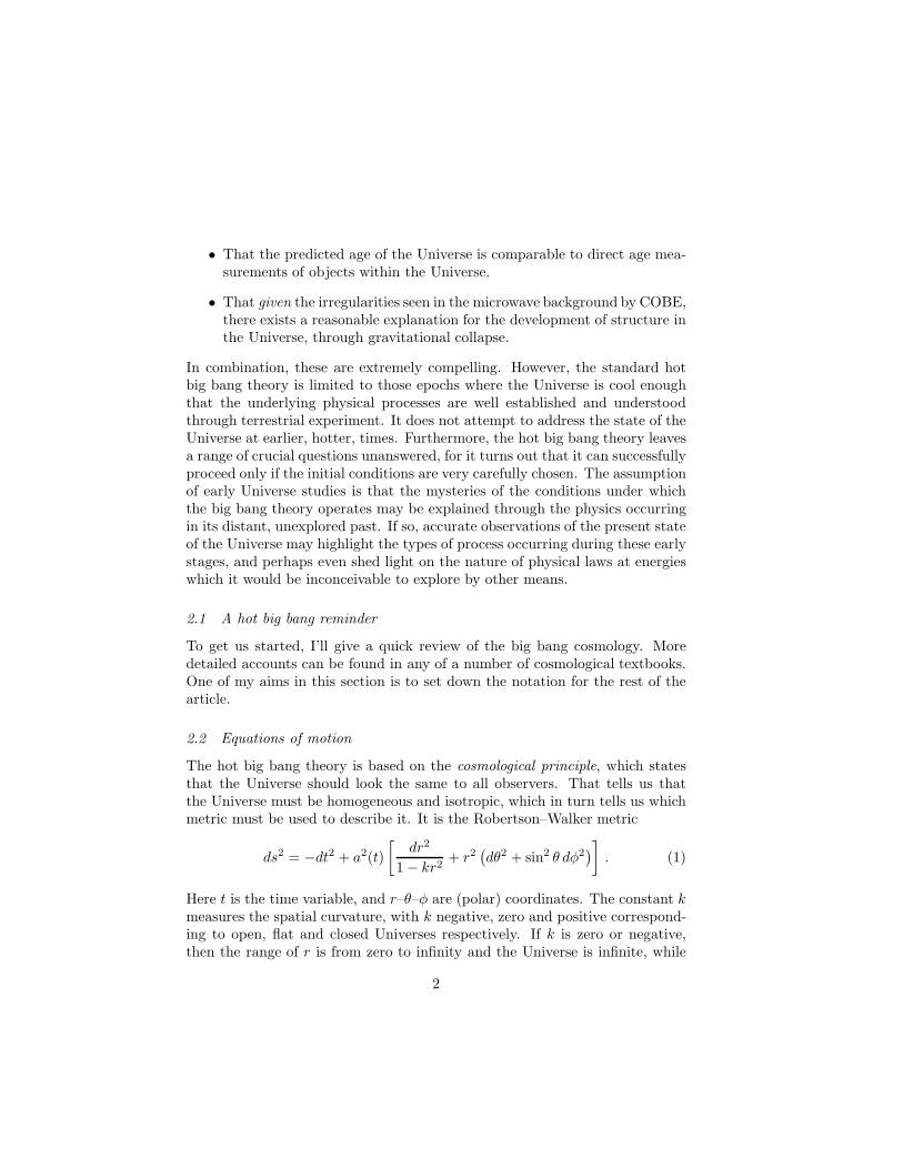
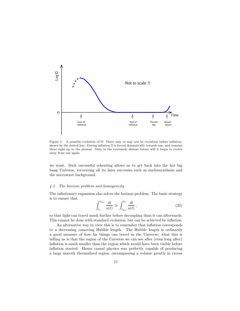
Inflation solves the flatness problem more or less by definition (so that at leastany classical, as opposed to quantum, solution of the problem will fall under theumbrella of the inflationary definition). From the middle condition, inflationis precisely the condition that Ω is forced towards one rather than away fromit. As we shall see, this typically happens very rapidly. A short period of suchbehaviour won’t do us any good, as the subsequent non-inflationary behaviour(in particular the standard big bang evolution from nucleosynthesis onwards)will take us away from flatness again, but all will be well provided we haveenough inflation that Ω is moved extremely close to one during the inflationaryepoch. If it is close enough, then it will stay very close to one right to thepresent, despite being repelled from one for all the post-inflationary period.Obtaining sufficient inflation to perform this task is actually fairly easy. Aschematic illustration of this behaviour is shown in Figure 1.

In the above discussion, I have ignored a possible cosmological constantcontribution, but if present it modifies the Friedmann equation to

|Ω + ΩΛ − 1| =|k|a2H2

, (31)

and so it is Ω + ΩΛ which is forced to one. In general, it is spatial flatness(k ≃ 0) that we are driven towards, not a critical matter density.

4.2 Relic abundances

The rapid expansion of the inflationary stage rapidly dilutes the unwantedrelic particles, because the energy density during inflation falls off more slowly(as a−2 or slower) than the relic particle density. Very quickly their densitybecomes negligible.

This resolution can only work if, after inflation, the energy density ofthe Universe can be turned into conventional matter without recreating theunwanted relics. This can be achieved by ensuring that during the conversion,known as reheating, the temperature never gets hot enough again to allowtheir thermal recreation. Then reheating can generate solely the things which

10

0

Start ofinflation

Time

inflationEnd of Present

day futuredistant

Log

Ω

Not to scale !!

Figure 1: A possible evolution of Ω. There may or may not be evolution before inflation,shown by the dotted line. During inflation Ω is forced dramatically towards one, and remainsthere right up to the present. Only in the extremely distant future will it begin to evolveaway from one again.

we want. Such successful reheating allows us to get back into the hot bigbang Universe, recovering all its later successes such as nucleosynthesis andthe microwave background.

4.3 The horizon problem and homogeneity

The inflationary expansion also solves the horizon problem. The basic strategyis to ensure that

∫ tdec

t∗

dt

a(t)≫

∫ t0

tdec

dt

a(t), (32)

so that light can travel much further before decoupling than it can afterwards.This cannot be done with standard evolution, but can be achieved by inflation.

An alternative way to view this is to remember that inflation correspondsto a decreasing comoving Hubble length. The Hubble length is ordinarilya good measure of how far things can travel in the Universe; what this istelling us is that the region of the Universe we can see after (even long after)inflation is much smaller than the region which would have been visible beforeinflation started. Hence causal physics was perfectly capable of producinga large smooth thermalized region, encompassing a volume greatly in excess

11

COMOVING

smooth patch

now

end

Hubble length

start

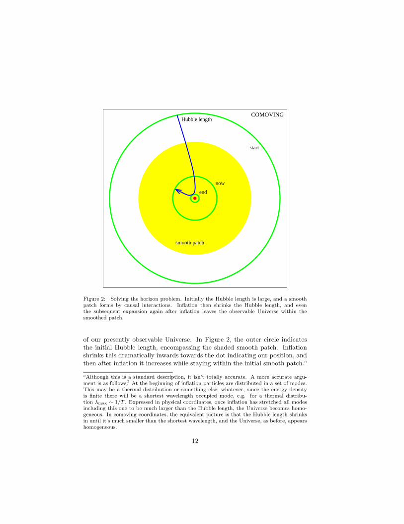
Figure 2: Solving the horizon problem. Initially the Hubble length is large, and a smoothpatch forms by causal interactions. Inflation then shrinks the Hubble length, and eventhe subsequent expansion again after inflation leaves the observable Universe within thesmoothed patch.

of our presently observable Universe. In Figure 2, the outer circle indicatesthe initial Hubble length, encompassing the shaded smooth patch. Inflationshrinks this dramatically inwards towards the dot indicating our position, andthen after inflation it increases while staying within the initial smooth patch.c

cAlthough this is a standard description, it isn’t totally accurate. A more accurate argu-ment is as follows.2 At the beginning of inflation particles are distributed in a set of modes.This may be a thermal distribution or something else; whatever, since the energy densityis finite there will be a shortest wavelength occupied mode, e.g. for a thermal distribu-tion λmax ∼ 1/T . Expressed in physical coordinates, once inflation has stretched all modesincluding this one to be much larger than the Hubble length, the Universe becomes homo-geneous. In comoving coordinates, the equivalent picture is that the Hubble length shrinksin until it’s much smaller than the shortest wavelength, and the Universe, as before, appearshomogeneous.

12

Equally, causal processes would be capable of generating irregularities inthe Universe on scales greatly exceeding our presently observable Universe,provided they happened at an early enough time that those scales were withincausal contact. This will be explored in detail later.

5 Modelling the Inflationary Expansion

We have seen that a period of accelerated expansion — inflation — is sufficientto resolve a range of cosmological problems. But we need a plausible scenariofor driving such an expansion if we are to be able to make proper calculations.This is provided by cosmological scalar fields.

5.1 Scalar fields and their potentials

In particle physics, a scalar field is used to represent spin zero particles. Ittransforms as a scalar (that is, it is unchanged) under coordinate transfor-mations. In a homogeneous Universe, the scalar field is a function of timealone.

In particle theories, scalar fields are a crucial ingredient for spontaneoussymmetry breaking. The most famous example is the Higgs field which breaksthe electro-weak symmetry, whose existence is hoped to be verified at the LargeHadron Collider at CERN when it commences experiments next millennium.Scalar fields are also expected to be associated with the breaking of othersymmetries, such as those of Grand Unified Theories, supersymmetry etc.

• Any specific particle theory (eg GUTS, superstrings) contains scalarfields.

• No fundamental scalar field has yet been observed.

• In condensed matter systems (such as superconductors, superfluid he-lium etc) scalar fields are widely observed, associated with any phasetransition. People working in that subject normally refer to the scalarfields as ‘order parameters’.

The traditional starting point for particle physics models is the action,which is an integral of the Lagrange density over space and time and fromwhich the equations of motion can be obtained. As an intermediate step,one might write down the energy–momentum tensor, which sits on the right-hand side of Einstein’s equations. Rather than begin there, I will take as mystarting point expressions for the effective energy density and pressure of ahomogeneous scalar field, which I’ll call φ. These are obtained by comparison

13

of the energy–momentum tensor of the scalar field with that of a perfect fluid,and are

ρφ =1

2φ2 + V (φ) (33)

pφ =1

2φ2 − V (φ) . (34)

One can think of the first term in each as a kinetic energy, and the secondas a potential energy. The potential energy V (φ) can be thought of as aform of ‘configurational’ or ‘binding’ energy; it measures how much internalenergy is associated with a particular field value. Normally, like all systems,scalar fields try to minimize this energy; however, a crucial ingredient whichallows inflation is that scalar fields are not always very efficient at reachingthis minimum energy state.

Note in passing that a scalar field cannot in general be described by anequation of state; there is no unique value of p that can be associated witha given ρ as the energy density can be divided between potential and kineticenergy in different ways.

In a given theory, there would be a specific form for the potential V (φ),at least up to some parameters which one could hope to measure (such as theeffective mass and interaction strength of the scalar field). However, we are notpresently in a position where there is a well established fundamental theorythat one can use, so, in the absence of such a theory, inflation workers tendto regard V (φ) as a function to be chosen arbitrarily, with different choicescorresponding to different models of inflation (of which there are many). Someexample potentials are

V (φ) = λ(

φ2 −M2)2

Higgs potential (35)

V (φ) = 1

2m2φ2 Massive scalar field (36)

V (φ) = λφ4 Self-interacting scalar field (37)

The strength of this approach is that it seems possible to capture many ofthe crucial properties of inflation by looking at some simple potentials; oneis looking for results which will still hold when more ‘realistic’ potentials arechosen. Figure 3 shows such a generic potential, with the scalar field displacedfrom the minimum and trying to reach it.

5.2 Equations of motion and solutions

The equations for an expanding Universe containing a homogeneous scalar fieldare easily obtained by substituting Eqs. (33) and (34) into the Friedmann and

14

V( )

φ

φ

Figure 3: A generic inflationary potential.

fluid equations, giving

H2 =8π

3m2Pl

[

V (φ) +1

2φ2

]

, (38)

φ+ 3Hφ = −V ′(φ) , (39)

where prime indicates d/dφ. Here I have ignored the curvature term k, since weknow that by definition it will quickly become negligible once inflation starts.This is done for simplicity only; there is no obstacle to including that term.

Since

a > 0 ⇐⇒ p < −ρ3⇐⇒ φ2 < V (φ) (40)

we will have inflation whenever the potential energy dominates. This shouldbe possible provided the potential is flat enough, as the scalar field would thenbe expected to roll slowly. The potential should also have a minimum in whichinflation can end.

The standard strategy for solving these equations is the slow-roll ap-

proximation (SRA); this assumes that a term can be neglected in each of theequations of motion to leave the simpler set

H2 ≃ 8π

3m2Pl

V (41)

3Hφ ≃ −V ′ (42)

15

If we define slow-roll parameters 3

ǫ(φ) =m2

Pl

16π

(

V ′

V

)2

; η(φ) =m2

Pl

8π

V ′′

V, (43)

where the first measures the slope of the potential and the second the curvature,then necessary conditions for the slow-roll approximation to hold are d

ǫ≪ 1 ; |η| ≪ 1 . (44)

Unfortunately, although these are necessary conditions for the slow-roll ap-proximation to hold, they are not sufficient, since even if the potential is veryflat it may be that the scalar field has a large velocity. A more elaborate ver-sion of the SRA exists, based on the Hamilton–Jacobi formulation of inflation,4

which is sufficient as well as necessary.5

Note also that the SRA reduces the order of the system of equations byone, and so its general solution contains one less initial condition. It worksonly because one can prove 4,5 that the solution to the full equations possessesan attractor property, eliminating the dependence on the extra parameter.

5.3 The relation between inflation and slow-roll

As it happens, the applicability of the slow-roll condition is closely connectedto the condition for inflation to take place, and in many contexts the conditionscan be regarded as equivalent. Let’s quickly see why.

The inflationary condition a > 0 is satisfied for a much wider range of be-haviours than just (quasi-)exponential expansion. A classic example is power-law inflation a ∝ tp for p > 1, which is an exact solution for an exponentialpotential

V (φ) = V0 exp

[

−√

16π

p

φ

mPl

]

. (45)

We can manipulate the condition for inflation as

a

a= H +H2 > 0

⇐⇒ − H

H2< 1

∼⇐⇒ m2

Pl

16π

(

V ′

V

)2

< 1

dNote that ǫ is positive by definition, whilst η can have either sign.

16

where the last manipulation uses the slow-roll approximation. The final con-dition is just the slow-roll condition ǫ < 1, and hence

Slow-roll =⇒ Inflation

Inflation will occur when the slow-roll conditions are satisfied (subject to somecaveats on whether the ‘attractor’ behaviour has been attained.5)

However, the converse is not strictly true, since we had to use the SRA inthe derivation. However, in practice

Inflation∼

=⇒ ǫ < 1

Prolonged inflation∼

=⇒ η < 1

The last condition arises because unless the curvature of the potential is small,the potential will not be flat for a wide enough range of φ.

5.4 The amount of inflation

The amount of inflation is normally specified by the logarithm of the amountof expansion, the number of e-foldings N , given by

N ≡ lna(tend)

a(tinitial)=

∫ te

ti

H dt , (46)

≃ − 8π

m2Pl

∫ φe

φi

V

V ′dφ , (47)

where the final step uses the SRA. Notice that the amount of inflation betweentwo scalar field values can be calculated without needing to solve the equationsof motion, and also that it is unchanged if one multiplies V (φ) by a constant.

The minimum amount of inflation required to solve the various cosmo-logical problems is about 70 e-foldings, i.e. an expansion by a factor of 1030.Although this looks large, inflation is typically so rapid that most inflationmodels give much more.

5.5 A worked example: polynomial chaotic inflation

The simplest inflation model 6 arises when one chooses a polynomial potential,such as that for a massive but otherwise non-interacting field, V (φ) = m2φ2/2where m is the mass of the scalar field. With this potential, the slow-rollequations are

3Hφ+m2φ = 0 ; H2 =4πm2φ2

3m2Pl

, (48)

17

and the slow-roll parameters are

ǫ = η =m2

Pl

4πφ2. (49)

So inflation can proceed provided |φ| > mPl/√

4π, i.e. as long as we are not toclose to the minimum.

The slow-roll equations are readily solved to give

φ(t) = φi −mmPl√

12πt , (50)

a(t) = ai exp

[

√

4π

3

m

mPl

(

φit−mmPl√

48πt2

)

]

, (51)

(where φ = φi and a = ai at t = 0) and the total amount of inflation is

Ntot = 2πφ2

i

m2

Pl

− 1

2. (52)

This last equation can be obtained from the solution for a, but in fact is moreeasily obtained directly by integrating Eq. (47), for which one needn’t botherto solve the equations of motion.

In order for classical physics to be valid we require V ≪ m4

Pl, but it is

still easy to get enough inflation provided m is small enough. As we shalllater see, m is in fact required to be small from observational limits on thesize of density perturbations produced, and we can easily get far more thanthe minimum amount of inflation required to solve the various cosmologicalproblems we originally set out to solve.

5.6 Reheating after inflation

During inflation, all matter except the scalar field (usually called the inflaton)is redshifted to extremely low densities. Reheating is the process wherebythe inflaton’s energy density is converted back into conventional matter afterinflation, re-entering the standard big bang theory.

Once the slow-roll conditions break down, the scalar field switches frombeing overdamped to being underdamped and begins to move rapidly on theHubble timescale, oscillating at the bottom of the potential. As it does so, itdecays into conventional matter. The details of reheating are an important areaof research in inflationary cosmology at the moment for several reasons, butare not important for the generation and evolution of density perturbations

18

which is the main focus of the remainder of this article. Consequently, I’lljust note that recently there has been quite a dramatic change of view asto how reheating takes place. Traditional treatments (e.g. as given in Kolb& Turner 7) added a phenomenological decay term; this was constrained tobe very small and hence reheating was viewed as being very inefficient. Thisallowed substantial redshifting to take place after the end of inflation and beforethe Universe returned to thermal equilibrium; hence the reheat temperaturewould be lower, by several orders of magnitude, than suggested by the energydensity at the end of inflation.

This picture is radically revised in work by Kofman, Linde & Starobinsky8

(see also Ref. 9), who suggest that the decay can undergo broad parametricresonance, with extremely efficient transfer of energy from the coherent oscil-lations of the inflaton field. This initial transfer has been dubbed preheating.With such an efficient start to the reheating process, it now appears possiblethat the reheating epoch may be very short indeed and hence that most of theenergy density in the inflaton field at the end of inflation may be available forconversion into thermalized form.

5.7 The range of inflation models

Over the last fifteen years or so a great number of inflationary models havebeen devised, both with and without reference to specific underlying particletheories. Here I will discuss a very small subset of the models which have beenintroduced, just to give you a flavour of the variety. At the moment particlephysics model building of inflation is undergoing a renaissance, and a detailedsnapshot of the current situation can be found in the review of Lyth & Riotto.10

However, as we shall be discussing in the next section, observations havegreat prospects for distinguishing between the different inflationary models.By far the best type of observation for this purpose appears to be high res-olution satellite microwave background anisotropy observations, and we arefortunate that two proposals have been approved — NASA has funded theMAP satellite 11 for launch around 2000, and ESA has approved the Planck

satellite 12 for launch some later. These satellites should offer very strong dis-crimination between the inflation models I shall now discuss. Indeed, it mayeven be possible to attempt a more challenging type of observation — onewhich is independent of the particular inflationary model and hence begins totest the idea of inflation itself.

Chaotic inflation models

This is the standard type of inflation model.6 The ingredients are

19

• A single scalar field, rolling in ...

• A potential V (φ), which in some regions satisfies the slow-roll conditions,while also possessing a minimum with zero potential in which inflationis to end.

• Initial conditions well up the potential, due to large fluctuations at thePlanck era.

There are a large number of models of this type. Some are

Polynomial chaotic inflation V (φ) = 1

2m2φ2

V (φ) = λφ4

Power-law inflation V (φ) = V0 exp(√

16πp

φmPl

)

‘Natural’ inflation V (φ) = V0[1 + cos φf ]

Intermediate inflation V (φ) ∝ φ−β

Some of these actually do not satisfy the condition of a minimum in whichinflation ends; they permit inflation to continue forever. However, we shall seepower-law inflation arising in a more satisfactory context shortly.

Multi-field theories

A recent trend in inflationary model building has been the exploration of mod-els with more than one scalar field. The classic example is the hybrid inflationmodel,13 which seems particularly promising for particle physics model build-ing. The simplest version has a potential with two fields φ and ψ of the form

V (φ, ψ) =λ

4

(

ψ2 −M2)2

+1

2m2φ2 +

1

2λ′φ2ψ2 . (53)

which is illustrated in Figure 4. When φ2 is large, the minimum of the potentialin the ψ-direction is at ψ = 0. The field rolls down this ‘channel’ until it reachesφ2

inst= λM2/λ′, at which point ψ = 0 becomes unstable and the field rolls

into one of the true minima at φ = 0 and ψ = ±M .While in the ‘channel’, which is where all the interesting behaviour takes

place, this is just like a single field model with an effective potential for φ ofthe form

Veff(φ) =λ

4M4 +

1

2m2φ2 . (54)

This is a fairly standard form, the unusual thing being the constant term, whichwould not normally be allowed as it would give a present-day cosmological

20

φinst

φ

ψ

V

Figure 4: The potential for the hybrid inflation model. The field rolls down the channelat ψ = 0 until it reaches the critical φ value, then falls off the side to the true minimum atφ = 0 and ψ = ±M .

constant. The most interesting regime is where that constant dominates, andit gives quite an unusual phenomenology. In particular, the energy densityduring inflation can be much lower than normal while still giving suitablylarge density perturbations, and secondly the field φ can be rolling extremelyslowly which is of benefit to particle physics model building.

Within the more general class of two and multi-field inflation models, it isquite common for only one field to be dynamically important, as in the hybridinflation model — this effectively reduces the situation back to the single fieldcase of the previous subsection. However, it may also be possible to havemore than one important dynamical degree of freedom. In that case thereis no attractor behaviour giving a unique route into the potential minimum,as in the single field case; for example, if the potential is of the form of anasymmetric bowl one could roll into the base down any direction. In thatsituation, the model loses some of its predictive power, because the late-timebehaviour is not independent of the initial conditions.e

eOf course, there is no requirement that the ‘true’ physical theory does have predictivepower, but it would be unfortunate for us if it does not.

21

Beyond general relativity

Rather than introduce an explicit scalar field to drive inflation, some theoriesmodify the gravitational sector of the theory into something more complicatedthan general relativity.14 Examples are

• Higher derivative gravity (R+R2 + · · ·).

• Jordan–Brans–Dicke theory.

• Scalar–tensor gravity.

The last two are theories where the gravitational constant may vary (indeedJordan–Brans–Dicke theory is a special case of scalar–tensor gravity).

However, a clever trick, known as the conformal transformation,15 allowssuch theories to be rewritten as general relativity plus one or more scalar fieldswith some potential. Often, only one of those fields is dynamical which returnsus once more to the original chaotic inflation scenario!

The most famous example is extended inflation.16 In its original form,it transforms precisely into the power-law inflation model that we’ve alreadydiscussed, with the added bonus that it includes a proper method of endinginflation. Unfortunately though, this model is now ruled out by observations.3

Indeed, models of inflation based on altering gravity are much more constrainedthan other types, since we know a lot about gravity and how well general rel-ativity works,14 and many models of this kind are very vulnerable to observa-tions.

Open inflation

In the early 1990s, in the face of ever increasing evidence of a sub-criticalmatter density in the Universe, interest was refocussed on an idea which defiesthe original inflationary motivation and gives rise to a homogeneous but openUniverse from inflation.f Often in the past it has been declared that this iseither impossible or contrived; however, it can be readily achieved in modelswith quantum tunnelling from a false vacuum (a metastable state) followed bya second inflationary stage.17 The tunnelling creates a bubble, and, incredibly,the region inside the expanding bubble looks just like an open Universe, withthe bubble wall corresponding to the initial (coordinate) singularity. Thesemodels are normally referred to as ‘open inflation’ or ‘single-bubble’ models.So far it has turned out that such models are not all that easy to construct.

f That is, a genuinely open Universe with hyperbolic geometry and no cosmological constant.

22

These models are already very different from traditional inflation mod-els, and subsequently an even bolder idea has been proposed,18 that an openUniverse can be created via ‘tunnelling from nothing’ rather than from a pre-existing inflationary phase. As I write this remains controversial.

While both these types of open inflation models remain viable, they areconsiderably more complex than the standard inflation models, and at the mo-ment not that well motivated as although observations continue to favour a lowmatter density, they also favour spatial flatness reintroduced by a cosmologicalconstant. Therefore from now on I will restrict discussion to the single-fieldchaotic inflation models.

5.8 Recap

The main points of this long section were the following.

• Cosmological scalar fields, which were introduced long before inflationwas thought of, provide a natural framework for inflation.

• Despite a wide range of motivations, most inflationary models are dy-namically equivalent to general relativity plus a single scalar field withsome potential V (φ).

• Within this framework, solutions describing inflation are easily found.Indeed, for many of the properties (amount of expansion, for example),we do not even need to solve the equations of motion.

With this information under our belts, we are now able to discuss the strongestmotivation for the inflationary cosmology — that it is able to provide an ex-planation for the origin of structure in the Universe.

6 Density Perturbations and Gravitational Waves

In modern terms, by far the most important property of inflationary cosmol-ogy is that it produces spectra of both density perturbations and gravita-tional waves. The density perturbations may be responsible for the formationand clustering of galaxies, as well as creating anisotropies in the microwavebackground radiation. The gravitational waves do not affect the formation ofgalaxies, but as we shall see may contribute extra microwave anisotropies onthe large angular scales sampled by the COBE satellite.19,20 An alternativeterminology for the density perturbations is scalar perturbations and for thegravitational waves is tensor perturbations, the terminology referring to theirtransformation properties.

23

Studies of large-scale structure typically make some assumption about theinitial form of these spectra. Usually gravitational waves are assumed notto be present, and the density perturbations to take on a simple form suchas the scale-invariant Harrison–Zel’dovich spectrum, or a scale-free power-lawspectrum. It is clearly highly desirable to have a theory which predicts theforms of the spectra. There are presently two rival models which do this,cosmological inflation and topological defects. At present inflation is favouredboth on observational grounds and because it provides a simpler frameworkfor understanding the evolution of structure

6.1 Production during inflation

The ability of inflation to generate perturbations on large scales comes fromthe unusual behaviour of the Hubble length during inflation, namely that (bydefinition) the comoving Hubble length decreases. When we talk about large-scale structure, we are primarily interested in comoving scales, as to a firstapproximation everything is dragged along with the expansion. The qualita-tive behaviour of irregularities is governed by their scale in comparison to thecharacteristic scale of the Universe, the Hubble length.

In the big bang Universe the comoving Hubble length is always increas-ing, and so all scales are initially much larger than it, and hence unable to beaffected by causal physics. Once they become smaller than the Hubble length,they remain so for all time. In the standard scenarios, COBE sees perturba-tions on large scales at a time when they were much bigger than the Hubblelength, and hence no mechanism could have created them.

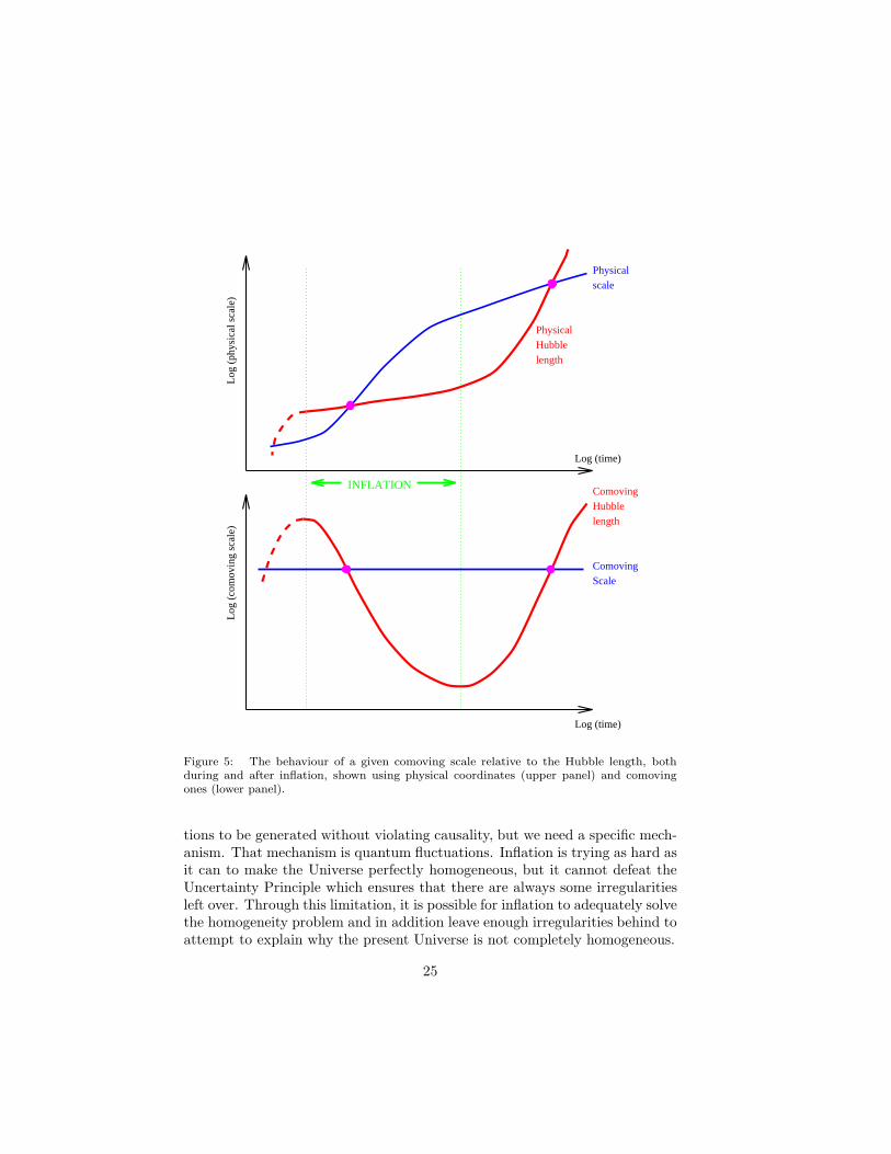
Inflation reverses this behaviour, as seen in Figure 5. Now a given comov-ing scale has a more complicated history. Early on in inflation, the scale couldbe well inside the Hubble length, and hence causal physics can act, both togenerate homogeneity to solve the horizon problem and to superimpose smallperturbations. Some time before inflation ends, the scale crosses outside theHubble radius (indicated by a circle in the lower panel of Figure 5) and causalphysics becomes ineffective. Any perturbations generated become imprinted,or, in the usual terminology, ‘frozen in’. Long after inflation is over, the scalescross inside the Hubble radius again. Perturbations are created on a very widerange of scales, but the most readily observed ones range from about the sizeof the present Hubble radius (i.e. the size of the presently observable Universe)down to a few orders of magnitude less. On the scale of Figure 5, all interest-ing comoving scales lie extremely close together, and cross the Hubble radiusduring inflation very close together.

It’s all very well to realize that the dynamics of inflation permits perturba-

24

length

Physicalscale

Comoving

Log

(co

mov

ing

scal

e)

Hubblelength

ComovingScale

PhysicalHubble

INFLATION

Log (time)

Log (time)

Log

(ph

ysic

al s

cale

)

Figure 5: The behaviour of a given comoving scale relative to the Hubble length, bothduring and after inflation, shown using physical coordinates (upper panel) and comovingones (lower panel).

tions to be generated without violating causality, but we need a specific mech-anism. That mechanism is quantum fluctuations. Inflation is trying as hard asit can to make the Universe perfectly homogeneous, but it cannot defeat theUncertainty Principle which ensures that there are always some irregularitiesleft over. Through this limitation, it is possible for inflation to adequately solvethe homogeneity problem and in addition leave enough irregularities behind toattempt to explain why the present Universe is not completely homogeneous.

25

The size of the irregularities depends on the energy scale at which inflationtakes place. It is outside the scope of these lectures to describe in detailhow this calculation is performed (see e.g. Ref. 21 for a reasonably accessibledescription); I’ll just briefly outline the necessary steps and then quote theresult, which we can go on to apply.

(a) Perturb the scalar field φ = φ(t) + δφ(x, t)(b) Expand in comoving wavenumbers δφ =

∑

(δφ)keik.x

(c) Linearized equation for classical evolution(d) Quantize theory(e) Find solution with initial condition giving

flat space quantum theory (k ≫ aH)(f) Find asymptotic value for k ≪ aH 〈|δφk|2〉 = H2/2k3

(g) Relate field perturbation to metric R = H δφ/φor curvature perturbation

Some important points are

• The details of this calculation are extremely similar to those used tocalculate the Casimir effect (a quantum force between parallel plates),which has been tested in the laboratory.

• The calculation itself is not controversial, though some aspects of itsinterpretation (in particular concerning the quantum to classical transi-tion) are.

• Exact analytic results are not known for general inflation models (thoughlinear theory results for arbitrary models are readily calculated numer-ically 22). The results I’ll be quoting will be lowest-order in the SRA,which is good enough for present observations.

• Results are known to second-order in slow-roll for arbitrary inflatonpotentials.23 Power-law inflation is the only standard model for whichexact results are known. In some other cases, high accuracy approxi-mations give better results (e.g. small-angle approximation in natural orhybrid inflation 23,24).

The formulae for the amplitude of density perturbations, which I’ll call

26

δH(k), and the gravitational waves, AG(k), are g

δH(k) =

√

512π

75

V 3/2

m3

Pl|V ′|

∣

∣

∣

∣

∣

k=aH

, (55)

AG(k) =

√

32

75

V 1/2

m2

Pl

∣

∣

∣

∣

∣

k=aH

. (56)

Here k is the comoving wavenumber; the perturbations are normally analyzedvia a Fourier expansion into comoving modes. The right-hand sides of theabove equations are to be evaluated at the time when k = aH during inflation,which for a given k corresponds to some particular value of φ. We see that theamplitude of perturbations depends on the properties of the inflaton potentialat the time the scale crossed the Hubble radius during inflation. The relevantnumber of e-foldings from the end of inflation is given by 2

N ≃ 62 − lnk

a0H0

+ numerical correction , (57)

where ‘numerical correction’ is a typically smallish (order a few) number whichdepends on the energy scale of inflation, the duration of reheating and so on.Normally it is a perfectly fine approximation to say that the scales of interestto us crossed outside the Hubble radius 60 e-foldings before the end of inflation.Then the e-foldings formula

N ≃ − 8π

m2

Pl

∫ φend

φ

V

V ′dφ , (58)

tells us the value of φ to be substituted into Eqs. (55) and (56).

6.2 A worked example

The easiest way to see what is going on is to work through a specific example,the m2φ2/2 potential which we already saw in Section 5.5. We’ll see that wedon’t even have to solve the evolution equations to get our predictions.

1. Inflation ends when ǫ = 1, so φend ≃ mPl/√

4π.

gThe precise normalization of the spectra is arbitrary, as are the number of powers of kincluded. I’ve made my favourite choice here (following Refs. 2,21), but whatever conventionis used the normalization factor will disappear in any physical answer. For reference, theusual power spectrum P (k) is proportional to kδ2

H(k).

27

2. We’re interested in 60 e-foldings before this, which from Eq. (52) givesφ60 ≃ 3mPl.

3. Substitute this in:

δH ≃ 12m

mPl

; AG ≃ 1.4m

mPl

4. Reproducing the COBE result requires25 δH ≃ 2×10−5 (provided AG ≪δH), so we need m ≃ 10−6mPl.

Because the required value of m is so small, that means it is easy to getsufficient inflation to solve the cosmological problems, without violating theclassicality condition V < m4

Pl. That implies only that φ < m2

Pl/m ≃ 106mPl,

and as Ntot ≃ 2πφ2/m2

Pl, we can get up to about 1013 e-foldings in principle.

This compares extremely favourably with the 70 or so actually required.

6.3 Observational consequences

Observations have moved on beyond us wanting to know the overall normal-ization of the potential. The interesting things are

1. The scale-dependence of the spectra.

2. The relative influence of the two spectra.

These can be neatly summarized using the slow-roll parameters ǫ and η wedefined earlier.3

The standard approximation used to describe the spectra is the power-

law approximation, where we take

δ2H(k) ∝ kn−1 ; A2

G(k) ∝ knG , (59)

where the spectral indices n and nG are given by

n− 1 =d ln δ2

H

d ln k; nG =

d lnA2G

d ln k. (60)

The power-law approximation is usually valid because only a limited rangeof scales are observable, with the range 1 Mpc to 104 Mpc corresponding to∆ ln k ≃ 9.

The crucial equation we need is that relating φ values to when a scale kcrosses the Hubble radius, which from Eq. (58) is

d ln k

dφ=

8π

m2Pl

V

V ′. (61)

28

MODEL POTENTIAL n R

Polynomial φ2 0.97 0.1chaotic inflation φ4 0.95 0.2Power-law inflation exp(−λφ) any n < 1 2π(1 − n)‘Natural’ inflation 1 + cos(φ/f) any n < 1 0Hybrid inflation (standard) 1 +Bφ2 1 0Hybrid inflation (extreme) 1 +Bφ2 1 < n < 1.15 ∼ 0

Table 1: The spectral index and gravitational wave contribution for a range of inflationmodels.

(since within the slow-roll approximation k ≃ expN). Direct differentiationthen yields 3

n = 1 − 6ǫ+ 2η , (62)

nG = −2ǫ , (63)

where now ǫ and η are to be evaluated on the appropriate part of the potential.Finally, we need a measure of the relevant importance of density perturba-

tions and gravitational waves. The natural place to look is the microwave back-ground; a detailed calculation which I cannot reproduce here (see e.g. Ref. 2)gives

R ≡ CGWℓ

CDPℓ

≃ 4πǫ . (64)

Here the Cℓ are the contributions to the microwave multipoles, in the usualnotation.h

From these expressions we immediately see

• If and only if ǫ≪ 1 and |η| ≪ 1 do we get n ≃ 1 and R ≃ 0.

• Because the coefficient in Eq. (64) is so large, gravitational waves canhave a significant effect even if ǫ is quite a bit smaller than one.

Table 1 shows the predictions for a range of inflation models. The infor-mation I’ve given you so far should be sufficient to allow you to reproducethem. Even the simplest inflation models can affect the large-scale structuremodelling at a level comparable to the present observational accuracy. Thepredictions of the different models will be wildly different as far as future high-accuracy observations are concerned.

hNamely, ∆T/T =∑

aℓmYℓm(θ, φ), Cℓ = 〈|aℓm|2〉.

29

Observations have some way to go before the power-law approximationbecomes inadequate. Consequently ...

• Slow-roll inflation adds two, and only two, new parameters to large-scalestructure.

• Although ǫ and η are the fundamental parameters, it is best to take themas n and R.

• Inflation models predict a wide range of values for these. Hence inflationmakes no definite prediction for large-scale structure.

• However, this means that large-scale structure observations, and espe-cially microwave background observations, can strongly discriminate be-tween inflationary models. When they are made, most existing inflationmodels will be ruled out.

6.4 Testing the idea of inflation

The moral of the previous section was that different inflation models lead tovery different models of structure formation, spanning a wide range of possi-bilities. That means, for example, that a definite measure of say the spectralindex n would rule out most inflation models. But it would always be possibleto find models which did give that value of n. Is there any way to try and testthe idea of inflation, independently of the model chosen?

The answer, in principle, is yes. In the previous section we introducedthree observables (in addition to the overall normalization), namely n, R andnG. However, they depend only on two fundamental parameters, namely ǫ andη.3 We can therefore eliminate ǫ and η to obtain a relation between observables,the consistency equation

R = −2πnG . (65)

This relation has been much discussed in the literature.26,21 It is independentof the choice of inflationary model (though it does rely on the slow-roll andpower-law approximations).

The idea of a consistency equation is in fact very general. The point is thatwe have obtained two continuous functions, δH(k) and AG(k), from a singlecontinuous function V (φ). This can only be possible if the functions δH(k) andAG(k) are related, and the equation quoted above is the simplest manifestationof such a relation.

Vindication of the consistency equation would be a remarkably convincingtest of the inflationary paradigm, as it would be highly unlikely that any other

30

production mechanism could entangle the two spectra in the way inflation does.Unfortunately though, measuring nG is a much more challenging observationaltask than measuring n or R and is likely to be beyond even next generationobservations. Indeed, this is a good point to remind the reader that even ifinflation is right, only one model can be right and it is perfectly possible (andmaybe even probable, see Ref. 27) that that model has a very low amplitude ofgravitational waves and that they will never be detected.

7 The inflationary origin of structure

At the summer school where these lectures were given, models of structureformation were described in detail by Joe Silk and for a detailed treatment Irefer you to his corresponding article. Here I will address those issues of directrelevance to the inflationary cosmology.

7.1 The parameters

The initial goal of structure formation studies is to accurately determine thefundamental parameters describing our Universe. So far I’ve stressed the threeinflationary parameters, δH, n and r, which describe the initial perturbationswhich inflation generates. However, except on very large scales where theyremain untouched by causal processes, we do not see the original perturbationsbut rather than perturbations after they have been processed by a variety ofphysical mechanisms. This processing depends on many quantities, all of whichmust be either fixed by assumption or determined from observations. A basiclist features four categories; the global dynamics, the way in which the mattercontent is divided amongst the different particle species, astrophysics effectssuch as reionization which would affect the microwave background photons,and the initial perturbation spectrum that we are here assuming comes frominflation. A possible list might look like this

1. Global dynamics

Hubble constant h ∗Spatial curvature k

2. Matter content

Baryons ΩB ∗Hot dark matter? ΩHDM

Cosmological constant? Λ (∗)

31

Massless species? g∗

3. Astrophysics

Reionization optical depth τ ∗

4. Initial perturbations

Amplitude δH(k = a0H0) ∗Spectral index n ∗Gravitational waves r

A cold dark matter contribution is not mentioned under matter content as itis assumed to take the value required to make the sums add up (i.e. to givethe right spatial curvature k given the other matter densities).

In this list, I’ve starred those parameters which need to be included in eventhe most minimal model, while the rest can be set to some particular value byassumption. I’ve partially starred the cosmological constant because althoughmost people would like to set it to zero, the observational case for a non-zerovalue is near to overwhelming.

7.2 The inflationary energy scale

The most solid observational result is the interpretation of the cosmic mi-crowave anisotropies seen by COBE as giving the amplitude of the initial powerspectrum. COBE is a particularly powerful probe because its large beam sizemakes it sensitive only to scales much larger than the horizon size when themicrowave background formed. The perturbations are therefore seen in theirprimordial form, and depend only on the initial perturbations and not all theother parameters. i

The COBE normalization requires the perturbation at the present Hubblescale, δH ≡ δH(k = a0H0), to be given by 25

δH ≃ 2 × 10−5 . (66)

Since

δ2H =32

75

V

m4Pl

1

ǫ, (67)

iThere is a residual dependence on Ω0 and Λ which determine the relation between themetric perturbations and the matter perturbations, and also the evolution of perturbations,but that is easily dealt with. I will assume critical density for simplicity.

32

then unless ǫ proves to be tiny (say much less than a hundredth) this will give

V 1/4 ≃ 10−3mPl ≃ 1016 GeV , (68)

at the time when observable scales crossed outside the horizon, pretty muchthe scale that particle physicists associate with Grand Unified Theories.

7.3 Beyond the energy scale

To go beyond the energy scale entails bringing together as wide a range ofobservations as possible to try and constrain the wide parameter family. Whenrestricted parameter sets are considered quite interesting constraints can bequoted, but these weaken once the parameter space is widened. Until recentlyno-one attempted a plausibly large parameter space, but recently Tegmark 28

considered a nine-parameter family of models, including the three inflationaryparameters, which is the first attempt to get to grips with the large families ofmodels that need to be considered for us to become convinced we are on theright track.

At present, observations are only quite weakly constraining concerningquantities beyond the inflationary energy scale. The spectral index is knownto lie near one, with the plausible range, depending on what parameters oneallows to vary, stretching from perhaps 0.8 to 1.2. As it happens, that is more orless the range which current inflation models tend to cover, and so most modelssurvive. The holy grail for inflation model building is an accurate measurementof n, say with an error bar of around 0.01 or better. Such a measurement wouldexclude the vast majority of the models currently under discussion. MAP, andcertainly Planck, ought to be able to deliver a measurement at around thisaccuracy level, and perhaps may even be able to see deviations from perfectpower-law behaviour.29,30

At the moment there is no evidence favouring a gravitational wave contri-bution to COBE, but equally the upper limit on such a contribution, perhapsaround r < 1 depending on other parameters (see Ref.31 for a recent analysis),is unable to rule out much in the way of interesting models (though it is a com-bination of the constraints on n and r that kills extended inflation). If such acontribution can be identified, it will be very strong support for inflation, butsince many models, especially of the currently-popular hybrid type, predict in-significant gravitational wave production, even the strongest achievable upperlimits may tell us nothing.

A particularly powerful test of inflation will be whether or not the mi-crowave anisotropy spectrum (the Cℓ) proves to contain an oscillatory peakstructure.32 Such a structure is evidence of phase coherence in the evolution of

33

perturbations (meaning that the perturbations of a given wavenumber are ata calculable phase of oscillation). Such phase coherence would indicate thatperturbations are entirely in the growing mode, which in turn implies that theyhave been evolving sufficiently long for the decaying mode to become negligi-ble. For modes around the horizon scale at decoupling, this implies that theywere already in place while well outside the horizon, which is a characteristicof inflationary perturbations (a characteristic not shared by topological de-fect models, for instance). This fairly qualitative test, if satisfied, will providestrong support for the inflationary paradigm, while if a multiple peak structureis not observed that will imply that the inflationary mechanism is not the solesource of perturbations in the Universe.

8 Summary

In this article I have introduced some of the facets of inflation in a fairly sim-ple manner. If you are interested in going beyond this, then the inflationaryproduction of perturbations is reviewed in Ref. 21, inflation and structure for-mation in Ref. 2 and particle physics aspects of inflation in Ref. 10.

At present, inflation is the most promising candidate theory for the originof perturbations in the Universe. Different inflation models lead to discerniblydifferent predictions for these perturbations, and hence high-accuracy mea-surements are able to distinguish between models, excluding either all or thevast majority of them.

Since its inception, the inflationary cosmology has been a gallery of differ-ent models, and the gallery has continually needed extension after extensionto house new acquisitions. In all the time up to the present, very few modelshave been discarded. However, the near future holds great promise to finallybegin to throw out inferior models, and, if the inflationary cosmology survivesas our model for the origin of structure, we can hope to be left with only anarrow range of models to choose between.

Acknowledgments

The author was supported in part by the Royal Society.

1. A. H. Guth, Phys. Rev. 23, 347 (1981).2. A. R. Liddle and D. H. Lyth, Phys. Rep 231, 1 (1993).3. A. R. Liddle and D. H. Lyth, Phys. Lett. B 291, 391 (1992).4. D. S. Salopek and J. R. Bond, Phys. Rev. D 42, 3936 (1990).5. A. R. Liddle, P. Parsons and J. D. Barrow, Phys. Rev. D 50, 7222

(1994).

34

6. A. D. Linde, Particle Physics and Inflationary Cosmology, Harwood Aca-demic, Chur, Switzerland (1990).

7. E. W. Kolb and M. S. Turner, The Early Universe, Addison-Wesley,Redwood City, California (1990) [updated paperback edition 1994].

8. L. Kofman, A. D. Linde and A. A. Starobinsky, Phys. Rev. Lett.73, 3195 (1994); A. D. Linde, astro-ph/9601004; L. Kofman, astro-ph/9605155.

9. Y. Shtanov, J. Traschen and R. Brandenberger, Phys. Rev. D 51, 5438(1995); D. Boyanovsky, M. D’Attanasio, H. de Vega, R. Holman, D.-S.Lee and A. Singh, Phys. Rev. D 52, 6805 (1995).

10. D. H. Lyth and A. Riotto, to appear, Phys. Rep., hep-ph/9807278.11. map home page at http://map.gsfc.nasa.gov/.12. Planck home page at http://astro.estec.esa.nl/Planck/.13. A. D. Linde, Phys. Lett. B 259, 38 (1991), Phys. Rev. D 49, 748

(1994); E. J. Copeland, A. R. Liddle, D. H. Lyth, E. D. Stewart and D.Wands, Phys. Rev. D 49, 6410 (1994).

14. C. M. Will, Theory and Experiment in Gravitational Physics, CambridgeUniversity Press (1993).

15. B. Whitt, Phys. Lett. 145B, 176 (1984); K. Maeda, Phys. Rev. D 39,3159 (1989); D. Wands, Class. Quant. Grav. 11, 269 (1994).

16. D. La and P. J. Steinhardt, Phys. Rev. Lett. 62, 376 (1989); E. W.Kolb, Physica Scripta T36, 199 (1991).

17. J. R. Gott, Nature 295, 304 (1982); M. Sasaki, T. Tanaka, K. Yamamotoand J. Yokoyama, Phys. Lett. B 317, 510 (1993); M. Bucher, A. S.Goldhaber and N. Turok, Phys. Rev. D 52, 3314; A. D. Linde and A.Mezhlumian, Phys. Rev. D 52, 6789 (1995).

18. S. W. Hawking and N. Turok, Phys. Lett. B 425, 25 (1998); A. D.Linde, Phys. Rev. D 58, 083514 (1998).

19. G. F. Smoot et al., Astrophys. J. 396, L1 (1992).20. C. L. Bennett et al., Astrophys. J. 464, L1 (1996).21. J. E. Lidsey, A. R. Liddle, E. W. Kolb, E. J. Copeland, T. Barriero and

M. Abney, Rev. Mod. Phys 69, 373 (1997).22. I. J. Grivell and A. R. Liddle, Phys. Rev. D 54, 7191 (1996).23. E. D. Stewart and D. H. Lyth, Phys. Lett. B 302, 171 (1993).24. J. Garcıa-Bellido and D. Wands, Phys. Rev. D 54, 7181 (1996).25. E. F. Bunn and M. White, Astrophys. J. 480, 6 (1987); E. F. Bunn, A.

R. Liddle and M. White, Phys. Rev. D 54, 5917R (1996).26. E. J. Copeland, E. W. Kolb, A. R. Liddle and J. E. Lidsey, Phys. Rev.

D 48, 2529 (1993), 49, 1840 (1994).27. D. H. Lyth, Phys. Rev. Lett. 78, 1861 (1997).

35

28. M. Tegmark, preprint astro-ph/9809201.29. A. Kosowsky and M. Turner, Phys. Rev. D 52, 1739 (1995).30. E. J. Copeland, I. J. Grivell and A. R. Liddle, Mon. Not. R. Astron.

Soc. 298, 1233 (1998).31. J. Zibin, D. Scott and M. White, preprint astro-ph/9901028.32. W. Hu and M. White, Phys. Rev. Lett. 77, 1687 (1996).

36