Embed Size (px)
Citation preview

LECTURE NOTES
Artifical Neural Networks
B. MEHLIG
(course home page)
Department of PhysicsUniversity of GothenburgGöteborg, Sweden 2018


PREFACE
These are lecture notes for my course on Artificial Neural Networks that Ihave given at Chalmers (FFR135) and Gothenburg University (FIM720). Thiscourse introduces the use of neural networks in machine learning: deeplearning, recurrent networks, reinforcement learning, and other supervisedand unsupervised machine-learning algorithms.
When I first developed my lectures, my main source was the book by Hertz,Krogh, and Palmer [1]. Other sources were the book by Haykin [2], as wellas the lecture notes of Horner [3]. My main sources for the Chapter on deeplearning were the deep-learning book by Goodfellow, Bengio & Courville [4],and the online-book by Nielsen [5].
I am grateful to Martin Cejka who typed the first version of my hand-written lecture notes and made most of the Figures, and to Erik Werner andHampus Linander for their interest and their help in preparing Chapter 7.I would like to thank also Johan Fries and Oleksandr Balabanov for imple-menting the algorithms described in Section 7.4. Johan Fries and MarinaRafajlovic made most of the exam questions. Finally many students – pastand present – pointed out misprints and errors and suggested improvements.I thank them all.


CONTENTS
Preface iii
Contents v
1 Introduction 11.1 Neural networks . . . . . . . . . . . . . . . . . . . . . . . . . . . . . . . . . . . . 31.2 McCulloch-Pitts neurons . . . . . . . . . . . . . . . . . . . . . . . . . . . . . . 41.3 Other models for neural computation . . . . . . . . . . . . . . . . . . . . . 61.4 Summary . . . . . . . . . . . . . . . . . . . . . . . . . . . . . . . . . . . . . . . . . 8
I Hopfield networks 9
2 Deterministic Hopfield networks 102.1 Associative memory problem . . . . . . . . . . . . . . . . . . . . . . . . . . . 102.2 Hopfield network . . . . . . . . . . . . . . . . . . . . . . . . . . . . . . . . . . . . 122.3 Energy function . . . . . . . . . . . . . . . . . . . . . . . . . . . . . . . . . . . . . 232.4 Spurious states . . . . . . . . . . . . . . . . . . . . . . . . . . . . . . . . . . . . . 262.5 Summary . . . . . . . . . . . . . . . . . . . . . . . . . . . . . . . . . . . . . . . . . 282.6 Exercises . . . . . . . . . . . . . . . . . . . . . . . . . . . . . . . . . . . . . . . . . . 282.7 Exam questions . . . . . . . . . . . . . . . . . . . . . . . . . . . . . . . . . . . . . 30
3 Stochastic Hopfield networks 353.1 Noisy dynamics . . . . . . . . . . . . . . . . . . . . . . . . . . . . . . . . . . . . . 353.2 Order parameters . . . . . . . . . . . . . . . . . . . . . . . . . . . . . . . . . . . 363.3 Mean-field theory . . . . . . . . . . . . . . . . . . . . . . . . . . . . . . . . . . . 383.4 Storage capacity . . . . . . . . . . . . . . . . . . . . . . . . . . . . . . . . . . . . 443.5 Beyond mean-field theory . . . . . . . . . . . . . . . . . . . . . . . . . . . . . 513.6 Summary . . . . . . . . . . . . . . . . . . . . . . . . . . . . . . . . . . . . . . . . . 523.7 Further reading . . . . . . . . . . . . . . . . . . . . . . . . . . . . . . . . . . . . . 533.8 Exercises . . . . . . . . . . . . . . . . . . . . . . . . . . . . . . . . . . . . . . . . . . 533.9 Exam questions . . . . . . . . . . . . . . . . . . . . . . . . . . . . . . . . . . . . . 54
4 Stochastic optimisation 554.1 Combinatorial optimisation problems . . . . . . . . . . . . . . . . . . . . 56

4.2 Energy functions . . . . . . . . . . . . . . . . . . . . . . . . . . . . . . . . . . . . 594.3 Simulated annealing . . . . . . . . . . . . . . . . . . . . . . . . . . . . . . . . . 604.4 Monte-Carlo simulation . . . . . . . . . . . . . . . . . . . . . . . . . . . . . . . 624.5 Summary . . . . . . . . . . . . . . . . . . . . . . . . . . . . . . . . . . . . . . . . . 644.6 Further reading . . . . . . . . . . . . . . . . . . . . . . . . . . . . . . . . . . . . . 644.7 Exercises . . . . . . . . . . . . . . . . . . . . . . . . . . . . . . . . . . . . . . . . . . 65
II Supervised learning 67
5 Perceptrons 685.1 A classification task . . . . . . . . . . . . . . . . . . . . . . . . . . . . . . . . . . 715.2 Iterative learning algorithm . . . . . . . . . . . . . . . . . . . . . . . . . . . . 745.3 Gradient-descent learning . . . . . . . . . . . . . . . . . . . . . . . . . . . . . 765.4 Multi-layer perceptrons . . . . . . . . . . . . . . . . . . . . . . . . . . . . . . . 785.5 Summary . . . . . . . . . . . . . . . . . . . . . . . . . . . . . . . . . . . . . . . . . 835.6 Further reading . . . . . . . . . . . . . . . . . . . . . . . . . . . . . . . . . . . . . 835.7 Exercises . . . . . . . . . . . . . . . . . . . . . . . . . . . . . . . . . . . . . . . . . . 835.8 Exam questions . . . . . . . . . . . . . . . . . . . . . . . . . . . . . . . . . . . . . 83
6 Stochastic gradient descent 896.1 Chain rule and error backpropagation . . . . . . . . . . . . . . . . . . . . 906.2 Stochastic gradient-descent algorithm . . . . . . . . . . . . . . . . . . . . 956.3 Recipes for improving the performance . . . . . . . . . . . . . . . . . . . 976.4 Summary . . . . . . . . . . . . . . . . . . . . . . . . . . . . . . . . . . . . . . . . . 1096.5 Further reading . . . . . . . . . . . . . . . . . . . . . . . . . . . . . . . . . . . . . 1096.6 Exercises . . . . . . . . . . . . . . . . . . . . . . . . . . . . . . . . . . . . . . . . . . 1106.7 Exam questions . . . . . . . . . . . . . . . . . . . . . . . . . . . . . . . . . . . . . 110
7 Deep learning 1157.1 How many hidden layers? . . . . . . . . . . . . . . . . . . . . . . . . . . . . . . 1157.2 Training deep networks . . . . . . . . . . . . . . . . . . . . . . . . . . . . . . . 1217.3 Convolutional networks . . . . . . . . . . . . . . . . . . . . . . . . . . . . . . . 1387.4 Learning to read handwritten digits . . . . . . . . . . . . . . . . . . . . . . 1427.5 Deep learning for object recognition . . . . . . . . . . . . . . . . . . . . . . 1507.6 Residual networks . . . . . . . . . . . . . . . . . . . . . . . . . . . . . . . . . . . 1537.7 Summary . . . . . . . . . . . . . . . . . . . . . . . . . . . . . . . . . . . . . . . . . 1557.8 Further reading . . . . . . . . . . . . . . . . . . . . . . . . . . . . . . . . . . . . . 158

7.9 Exercises . . . . . . . . . . . . . . . . . . . . . . . . . . . . . . . . . . . . . . . . . . 158
7.10 Exam questions . . . . . . . . . . . . . . . . . . . . . . . . . . . . . . . . . . . . . 159
8 Recurrent networks 161
8.1 Recurrent backpropagation . . . . . . . . . . . . . . . . . . . . . . . . . . . . 163
8.2 Backpropagation through time . . . . . . . . . . . . . . . . . . . . . . . . . . 166
8.3 Recurrent networks for machine translation . . . . . . . . . . . . . . . . 171
8.4 Summary . . . . . . . . . . . . . . . . . . . . . . . . . . . . . . . . . . . . . . . . . 174
8.5 Further reading . . . . . . . . . . . . . . . . . . . . . . . . . . . . . . . . . . . . . 174
8.6 Exercises . . . . . . . . . . . . . . . . . . . . . . . . . . . . . . . . . . . . . . . . . . 174
III Unsupervised learning 175
9 Unsupervised Hebbian learning 175
9.1 Oja’s rule . . . . . . . . . . . . . . . . . . . . . . . . . . . . . . . . . . . . . . . . . . 177
9.2 Competitive learning . . . . . . . . . . . . . . . . . . . . . . . . . . . . . . . . . 181
9.3 Kohonen’s algorithm . . . . . . . . . . . . . . . . . . . . . . . . . . . . . . . . . 183
9.4 Summary . . . . . . . . . . . . . . . . . . . . . . . . . . . . . . . . . . . . . . . . . 188
9.5 Exercises . . . . . . . . . . . . . . . . . . . . . . . . . . . . . . . . . . . . . . . . . . 189
9.6 Exam questions . . . . . . . . . . . . . . . . . . . . . . . . . . . . . . . . . . . . . 189
10 Radial basis-function networks 192
10.1 Separating capacity of a surface . . . . . . . . . . . . . . . . . . . . . . . . . 193
10.2 Radial basis-function networks . . . . . . . . . . . . . . . . . . . . . . . . . 196
10.3 Summary . . . . . . . . . . . . . . . . . . . . . . . . . . . . . . . . . . . . . . . . . 198
10.4 Further reading . . . . . . . . . . . . . . . . . . . . . . . . . . . . . . . . . . . . . 199
10.5 Exercises . . . . . . . . . . . . . . . . . . . . . . . . . . . . . . . . . . . . . . . . . . 199
10.6 Exam questions . . . . . . . . . . . . . . . . . . . . . . . . . . . . . . . . . . . . . 200
11 Reinforcement learning 202
11.1 Stochastic output units . . . . . . . . . . . . . . . . . . . . . . . . . . . . . . . 202
11.2 Associative reward-penalty algorithm . . . . . . . . . . . . . . . . . . . . . 204
11.3 Summary . . . . . . . . . . . . . . . . . . . . . . . . . . . . . . . . . . . . . . . . . 205
11.4 Further reading . . . . . . . . . . . . . . . . . . . . . . . . . . . . . . . . . . . . . 205

IV Appendix 207
12 Solutions 207
13 Some linear algebra 209

1
1 Introduction
The term neural networks refers to networks of neurons in the mammalianbrain. Neurons are its fundamental units of computation. In the brain theyare connected together in networks to process data. This is a very complextask, and the dynamics of neural networks in the mammalian brain is there-fore quite intricate. Inputs and outputs of each neuron vary as functions oftime, in the form of so-called spike trains, but also the network itself changes.We learn and improve our data-processing capacities by establishing recon-nections between neurons.
Neural-network algorithms are inspired by the architecture and the dy-namics of networks of neurons in the brain. Yet these algorithms use repre-sentations of neurons that are highly simplified, compared with real neurons.Nevertheless, the fundamental principle is the same: artificial neural net-works learn by re-connection. Such networks can perform a multitude ofinformation-processing tasks. They can learn to recognise structures in aset of training data and generalise what they have learnt to other data sets(supervised learning). A training set contains a list of input data sets, togetherwith a list of the corresponding target values that encode the properties of theinput data that the network is supposed to learn. To solve such associationtasks by artificial neural networks can work well when the new data sets aregoverned by the same principles that gave rise to the training data.
A prime example for a problem of this type is object recognition in images,for instance in the sequence of camera images of a self-driving car. Recentlythe use of neural networks for object recognition has exploded. There areseveral reasons for this strong interest. It is driven, first, by the acute needfor such algorithms in industry. Second, there are now much better imagedata bases available for training the networks. Third, there is better hard-ware (GPU processors), so that networks with many layers containing manyneurons can be efficiently trained (deep learning) [4, 6].
Another task where neural networks excel is machine translation. Thesenetworks are dynamical (recurrent) networks. They take an input sequence ofwords or sometimes single letters. As one feeds the inputs word by word, thenetwork outputs the words in the translated sentence. Recurrent networkscan be efficiently trained on large training sets of input sentences and theirtranslations. Google translate works in this way [7].

2 INTRODUCTION
axon
neural cell body
dendrites
Figure 1.1: Neurons in the cerebral cortex (outer layer of the cerebrum, thelargest and best developed part of the mammalian brain) of a macaque, an Asianmonkey. Reproduced by permission of brainmaps.org [9] under the CreativeCommons Attribution 3.0 License. The labels were added.
Artificial neural networks are good at analysing high-dimensional datawhere it may be difficult to determine a priori which properties are of interest.In this case one often relies on unsupervised learning algorithms where thenetwork learns without a training set. Instead it determines in terms of whichcategories the data can be analysed. In this way, artificial neural networkscan detect familiarity (which input patterns occur most often), clusters, andother structures in the input data. Unsupervised-learning algorithms workwell when there is redundancy in the input data that is not immediatelyobvious because the data is high dimensional.
In many problems some information about targets is known, yet incom-plete. In this case one uses algorithms that contain elements of both super-vised and unsupervised learning (reinforcement learning). Such algorithmsare used, for instance, in the software AlphaGo [8] that plays the game of go.
The different algorithms have much in common. They share the samebuilding blocks: the neurons are modeled as linear threshold units (McCulloch-Pitts neurons), and the learning rules are similar (Hebb’s rule). Closely relatedquestions arise also regarding the network dynamics. A little bit of noise (nottoo much!) can improve the performance, and ensures that the long-timedynamics approaches a steady state. This allows to analyse the convergenceof the algorithms using the central-limit theorem.
There are many connections to methods used in Mathematical Statistics,

NEURAL NETWORKS 3
input→ process → output
axon
cell body terminalsdendrites
synapses
Figure 1.2: Schematic image of a neuron. Dendrites receive input in the formof electrical signals, via synapses. The signals are processed in the cell bodyof the neuron. The output travels from the neural cell body to other neuronsthrough the axon.
such as Markov-chain Monte-Carlo algorithms and simulated annealing.Certain unsupervised learning algorithms are related to principal componentanalysis, others to clustering algorithms such as k -means clustering.
1.1 Neural networks
The mammalian brain consists of different regions that perform differenttasks. The cerebral cortex is the outer layer of the mammalian brain. We canthink of it as a thin sheet (about 2 to 5 mm thick) that folds upon itself toincrease its surface area. The cortex is the largest and best developed partof the Human brain. It contains large numbers of nerve cells, neurons. TheHuman cerebral cortex contains about 1010 neurons. They are linked togetherby nerve strands (axons) that branch and end in synapses. These synapsesare the connections to other neurons. The synapses connect to dendrites,branched extensions from the neural cell body designed to receive inputfrom other neurons in the form of electrical signals. A neuron in the Humanbrain may have thousands of synaptic connections with other neurons. Theresulting network of connected neurons in the cerebral cortex is responsiblefor perception of visual, audio, and sensory data, for language and imageprocessing, and for memory.
Figure 1.1 shows neurons in the cerebral cortex of the macaque, an Asianmonkey. The image displays a silver-stained cross section through the cere-

4 INTRODUCTION
Figure 1.3: Spike train in electrosensory pyramidal neuron in fish (eigenman-nia). Time series from Ref. [10]. Reproduced by permission of the publisher.
bral cortex. The brown and black parts are the neurons. One can distinguishthe cell bodies of the neural cells, their axons, and their dendrites.
Figure 1.2 shows a more schematic view of a neuron. Information isprocessed from left to right. On the left are the dendrites that receive signalsand connect to the cell body of the neuron where the signal is processed.The right part of the Figure shows the axon, through which the output is sentto the dendrites of other neurons.
Information is transmitted as an electrical signal. Figure 1.3 shows anexample of the time series of the electric potential for a pyramidal neuronin fish [10]. The time series consists of an intermittent series of electrical-potential spikes. Quiescent periods without spikes occur when the neuronis inactive, during spike-rich periods the neuron is active.
1.2 McCulloch-Pitts neurons
In artificial networks, the ways in which information is processed and signalsare transferred are highly simplified. The model we use nowadays for thecomputational unit, the artificial neuron, goes back to McCulloch and Pitts[11]. Rosenblatt [12, 13] described how to connect such units in artificialneural networks to process information. He referred to these networks asperceptrons.
In its simplest form, the model for the artificial neuron has only two states,active or inactive. The model works as a linear threshold unit: it processesall input signals and computes an output. If the output exceeds a giventhreshold then the state of the neuron is said to be active, otherwise inactive.

MCCULLOCH-PITTS NEURONS 5
n1(t )
n2(t )
n3(t )...
nN (t )
wi 1
wi 2
wi 3
wi N
µi
ni (t +1) = θH
�
∑Nj=1 wi j n j (t )−µi
�
Figure 1.4: Schematic diagram of a McCulloch-Pitts neuron. The index ofthe neuron is i , it receives inputs from N other neurons. The strength of theconnection from neuron j to neuron i is denoted by wi j . The function θH(b )(activation function) is the Heaviside function. It is equal to zero for b < 0 andequal to unity for b > 0. The threshold value for neuron i is denoted by µi . Theindex t = 0, 1, 2, 3, . . . labels the discrete time sequence of computation steps.
The model is illustrated in Figure 1.4.Neurons usually perform repeated computations, and one divides up
time into discrete time steps t = 0,1,2,3, . . .. The state of neuron number jat time step t is denoted by
n j (t ) =
¨
0 inactive ,
1 active .(1.1)
Given the signals n j (t ), neuron number i computes
ni (t +1) = θH
�
∑
j
wi j n j (t )−µi
�
. (1.2)
As written, this computation is performed for all neurons i in parallel, andthe outputs ni are the inputs to all neurons at the next time step, therefore theoutputs have the time argument t +1. These steps are repeated many times,resulting in time series of the activity levels of all neurons in the network,referred to as neural dynamics.
The procedure described above is called synchronous updating. An al-ternative is to choose a neuron randomly (or following a prescribed deter-ministic rule), and to update only this one, instead of all together. Thisscheme is called asynchronous updating. If there are N neurons, then onesynchronous step corresponds to N asynchronous steps, on average. This

6 INTRODUCTION
θH(b )
1
0 bFigure 1.5: Heaviside function.
difference in time scales is not the only difference between synchronous andasynchronous updating. In general the two schemes yield different neuraldynamics.
Now consider the details of the computation step Equation (1.2). Thefunction θH(b ) is the activation function. Its argument is often referred to asthe local field, bi (t ) =
∑
j wi j n j (t )−µi . Since the neurons can only assumethe states 0/1, the activation function is taken to be the Heaviside function,θH(b ) = 0 if b < 0 and θH(b ) = 1 if b > 0 (Figure 1.5). The Heaviside functionis not defined at b = 0. To avoid problems in our computer algorithms, weusually take θH(0) = 1.
Equation (1.2) shows that the neuron performs a weighted linear averageof the inputs n j (t ). The weights wi j are called synaptic weights. Here thefirst index, i , refers to the neuron that does the computation, and j labels allneurons that connect to neuron i . The connection strengths between dif-ferent pairs of neurons are in general different, reflecting different strengthsof the synaptic couplings. When the value of wi j is positive, we say that thecoupling is called excitatory. When wi j is negative, the connection is calledinhibitory. When wi j = 0 there is no connection:
wi j
> 0 excitatory connection ,
= 0 no connection from j to i
< 0 inhibitory connection .
(1.3)
Finally, the threshold for neuron i is denoted by µi .
1.3 Other models for neural computation
The dynamics defined by Equations (1.1) and (1.2) is just a caricature of thetime series of electrical signals in the cortex. For a start, the neural model
OTHER MODELS FOR NEURAL COMPUTATION 7
b
1g (b )
0
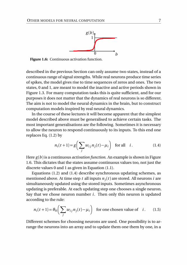
Figure 1.6: Continuous activation function.
described in the previous Section can only assume two states, instead of acontinuous range of signal strengths. While real neurons produce time seriesof spikes, the model gives rise to time sequences of zeros and ones. The twostates, 0 and 1, are meant to model the inactive and active periods shown inFigure 1.3. For many computation tasks this is quite sufficient, and for ourpurposes it does not matter that the dynamics of real neurons is so different.The aim is not to model the neural dynamics in the brain, but to constructcomputation models inspired by real neural dynamics.
In the course of these lectures it will become apparent that the simplestmodel described above must be generalised to achieve certain tasks. Themost important generalisations are the following. Sometimes it is necessaryto allow the neuron to respond continuously to its inputs. To this end onereplaces Eq. (1.2) by
ni (t +1) = g�
∑
j
wi j n j (t )−µi
�
for all i . (1.4)
Here g (b ) is a continuous activation function. An example is shown in Figure1.6. This dictates that the states assume continuous values too, not just thediscrete values 0 and 1 as given in Equation (1.1).
Equations (1.2) and (1.4) describe synchronous updating schemes, asmentioned above. At time step t all inputs n j (t ) are stored. All neurons i aresimultaneously updated using the stored inputs. Sometimes asynchronousupdating is preferable. At each updating step one chooses a single neuron.Say that we chose neuron number i . Then only this neuron is updatedaccording to the rule:
ni (t +1) = θH
�
∑
j
wi j n j (t )−µi
�
for one chosen value of i . (1.5)
Different schemes for choosing neurons are used. One possibility is to ar-range the neurons into an array and to update them one them by one, in a

8 INTRODUCTION
certain order (typewriter scheme). A second possibility is to choose randomlywhich neuron to update. This introduces stochasticity into the neural dy-namics. This is very important, and we will see that there are different ways ofintroducing stochasticity. Random asynchronous updating is one example.In many scientific problems it is advantageous to avoid stochasticity, whenrandomness is due to errors (multiplicative or additive noise) that diminishthe performance of the system. In neural-network dynamics, by contrast,stochasticity is often helpful, as we shall see below.
1.4 Summary
Artificial neural networks use a highly simplified model for the fundamen-tal computation unit, the neuron. In its simplest form, the model is just abinary threshold unit. The units are linked together by weights wi j , andeach unit computes a weighted average of its inputs. The network performsthese computations in sequence. Usually one considers discrete sequencesof computation time steps, t = 0,1,2,3, . . .. Either all neurons are updatedsimultaneously in one time step (synchronous updating), or only one chosenneuron is updated (asynchronous updating). Most neural-network algo-rithms are built using the model described in this Chapter.

9
PART I
HOPFIELD NETWORKS
The Hopfield network [14] is an artificial neural network that can recogniseor reconstruct images. Consider for example the binary images of digits inFigure 2.1. These images can be stored in the artificial neural network byassigning the weights wi j in a certain way (called Hebb’s rule). Then onefeeds a distorted image of one of the digits (Figure 2.2) to the network byassigning the initial states of the neurons in the network to the bits in thedistorted image. The idea is that the neural-network dynamics convergesto the correct undistorted digit. In this way the network can recognise theinput as a distorted image of the correct digit (retrieve this digit). The point isthat the network may recognise patterns with many bits very efficiently. Thisidea is quite old though. In the past such networks were used to performpattern recognition tasks. Today there are more efficient algorithms for thispurpose (Chapter 7).
Yet the first part of these lectures deals with Hopfield networks, for severalreasons. First, Hopfield nets form the basis for more recent algorithms suchas Boltzmann machines [2] and deep-belief networks [2]. Second, all otherneural-network algorithms discussed in these lectures are built from thesame building blocks and use learning rules that are closely related to Hebb’srule. Third, Hopfield networks can solve optimisation problems, and the re-sulting algorithm is closely related to Markov-chain Monte-Carlo algorithmswhich are much used for a wide range of problems in Physics and Mathe-matical Statistics. Fourth, and most importantly, a certain degree of noise(not too much) can substantially improve the performance of Hopfield net-works, and it is understood in detail why. The reason that so much is knownabout the role of noise in Hopfield networks is that they are closely relatedto stochastic systems studied in Physics, namely random magnets and spinglasses. The point is: understanding the effect of noise on the dynamics ofHopfield networks helps to analyse the performance of other neural-networkmodels.

10 DETERMINISTIC HOPFIELD NETWORKS
Figure 2.1: Binary representation of the digits 0 to 4. Each digit has 16× 10pixels.
2 Deterministic Hopfield networks
2.1 Associative memory problem
The pattern-recognition task described above (Figure 2.1) is an example ofan associative-memory problem: there are p images (patterns), each with Nbits. Examples for such sets of patterns are the letters in the alphabet, or thedigits shown in Figure 2.1. The different patterns are labeled by the index
µ = 1, . . . , p . The bits of pattern µ are denoted by x(µ)i . The index i labels
the bits of a given pattern, it ranges from 1 to N . The bits are binary: theycan take only the values 0 and 1, as illustrated in Figure 2.2. To determinethe generic properties of the algorithm, one often turns to random patterns
where each bit x(µ)i is chosen randomly. Each bit takes either value with
probability 12 , and different bits (in the same and in different patterns) are
independent. It is convenient to gather the bits of a pattern in a columnvector
x (µ) =
x(µ)1
x(µ)2...
x(µ)N
. (2.1)
In the following, vectors are written in bold math font.The first part of the problem is to store the patterns x (1) to x (p ). Second,
one feeds a test pattern x , a distorted version of one of the binary patternsin the problem. The aim is to determine which one of the stored patternsx (µ) most closely resembles x . The problem is, in other words, to associatethe test pattern with the closest one of the stored patterns. The formulation

ASSOCIATIVE MEMORY PROBLEM 11
xi = 1
xi = 0
i = 1, . . . , N
Figure 2.2: Binary image (N = 160) of the digit 0, and a distorted version of thesame image.
of the problem requires to define how close two given patterns are to eachother. One possibility is to use the Hamming distance. For patterns with 0/1bits, the Hamming distance hµ between the patterns x and x (µ) is defined as
hµ ≡N∑
i=1
�
x(µ)i (1− xi )+
�
1− x(µ)i
�
xi
�
. (2.2)
The Hamming distance equals the number of bits by which the patternsdiffer. Two patterns are identical if they have Hamming distance zero. For0/1 patterns, Equation (2.2) is equivalent to:
hµN=
1
N
N∑
i=1
�
x(µ)i − xi
�2. (2.3)
This means that the Hamming distance is given by the mean-squared error,summed over all bits. Note that the Hamming distance does not refer todistortions by translations, rotations, or shearing. An improved version ofthe distance involves taking the minimum distance between the patternssubject to all possible translations, rotations, and so forth.
In summary, the association task is to find the index ν for which theHamming distance hν is minimal, hν ≤ hµ for all µ= 1, . . . , p . How can onesolve this task using a neural network? One feeds the distorted pattern xwith bits xi into the network by assigning ni (t = 0) = xi . Assume that x is a

12 DETERMINISTIC HOPFIELD NETWORKS
+1
−1
sgn(b )
b
Figure 2.3: Signum function.
distorted version of x (ν). Now the idea is to find a set of weights wi j so thatthe network dynamics converges to the correct stored pattern:
ni (t )→ x (ν)i as t →∞ . (2.4)
Which weights to choose depends on the patterns x (µ), so the weights mustbe functions of x (µ). We say that we store these patterns in the network bychoosing the appropriate weights. If the network converges as in Equation(2.4), the pattern x (ν) is said to be an attractor in the space of all possiblestates of this network, the so-called configuration space or state space.
2.2 Hopfield network
Hopfield [14] used a network of McCulloch-Pitts neurons to solve the asso-ciative memory problem described in the previous Section. The states ofneuron i in the Hopfield network take the values
Si (t ) =
¨
−1 inactive ,
1 active ,(2.5)
instead of 0/1, because this simplifies the mathematical analysis as we shallsee. The transformation from ni ∈ {0, 1} to Si ∈ {−1, 1} is straightforward:
Si = 2ni −1 . (2.6)
The thresholds are transformed accordingly, θi = 2µi −∑
j wi j . For the bits
of the patterns we keep the symbol x(µ)i , but it is important to remember
that now x(µ)i = ±1. To ensure that the Si can only take the values ±1, the
activation function is taken to be the signum function (Figure 2.3).

HOPFIELD NETWORK 13
sgn(b ) =
¨
−1 b < 0 ,
+1, b > 0 .(2.7)
The signum function is not defined at b = 0. To avoid problems in ourcomputer algorithms we usually define sgn(0) = 1.
The asynchronous update rule takes the form
Si ← sgn�
∑
j
wi j Sj −θi
�
︸ ︷︷ ︸
≡bi
for one chosen value of i , (2.8)
As before i is the index of the chosen neuron. The arrow indicates that Si (t +1)is assigned the r.h.s of this equation evaluated at Sj (t ). The synchronousupdate rule reads
Si ← sgn�
∑
j
wi j Sj −θi
�
︸ ︷︷ ︸
≡bi
, (2.9)
where all bits are updated in parallel. In Eqs. (2.8) and (2.9) the argument ofthe activation function is denoted by bi , sometimes called the local field.
Now we need a strategy for choosing the weights wi j , so that the patternsx (µ) are attractors. If one feeds a pattern x close to x (ν) to the network, wewant the network to converge to x (ν)
S (t = 0) = x ≈ x (ν) ; S (t )→ x (ν) as t →∞ . (2.10)
This means that the network succeeds in correcting a small number of errors.If the number of errors is too large, the network may converge to anotherpattern. The region in configuration space around pattern x (ν) in which allpatterns converge to x (ν) is called the region of attraction of x (ν).
However, we shall see that it is in general very difficult to prove conver-gence according to Eq. (2.10). Therefore we try to answer a different questionfirst: if one feeds one of the undistorted patterns x (ν), does the network recog-nise that it is one of the stored, undistorted patterns? The network shouldnot make any changes to x (ν) because all bits are correct:
S (t = 0) = x (ν) ; S (t ) = x (ν) for all t = 0, 1, 2, . . . . (2.11)

14 DETERMINISTIC HOPFIELD NETWORKS
Even this question is in general difficult to answer. We therefore consider asimple limit of the problem first, namely p = 1. There is only one pattern torecognize, x (1). A suitable choice of weights wi j is given by Hebb’s rule
wi j =1
Nx (1)i x (1)j and θi = 0 . (2.12)
We say that the pattern x (1) is stored in the network by assigning the weightswi j using the rule (2.12). Note that the weights are symmetric, wi j =w j i . Tocheck that the rule (2.12) does the trick, feed the pattern to the network by
assigning Sj (t = 0) = x (1)j , and evaluate Equation (2.8):
N∑
j=1
wi j x (1)j =1
N
N∑
j=1
x (1)i x (1)j x (1)j =1
N
N∑
j=1
x (1)i . (2.13)
The last equality follows because x (1)j can only take the values ±1. The emptysum evaluates to N , so that
sgn� N∑
j=1
wi j x (1)j
�
= x (1)i . (2.14)
Recall that x(µ)i =±1, so that sgn(x (µ)i ) = x
(µ)i . Comparing Equation (2.14) with
the update rule (2.8) shows that the bits x (1)j of the pattern x (1) remain un-changed under the update, as required by Eq. (2.11). The network recognisesthe pattern as a stored one, so Hebb’s rule (2.12) does what we asked.
But does the network correct small errors? In other words, is the patternx (1) an attractor [Eq. (2.10)]? This question cannot be answered in general. Yetin practice Hopfield models work often very well! It is a fundamental insightthat neural networks may work well although it is impossible to strictly provethat their dynamics converges to the correct solution.
To illustrate the difficulties consider an example, a Hopfield network withp = 1 and N = 4 (Figure 2.4). Store the pattern x (1) shown in Figure 2.4 byassigning the weights wi j using Hebb’s rule (2.12). Now feed a distortedpattern x to the network that has a non-zero distance to x (1):
h1 =1
4
4∑
i=1
�
xi − x (1)i
�2> 0 . (2.15)

HOPFIELD NETWORK 15
1 2
3 4
(a) Network layout. The network has 4neurons, ◦. The arrows indicate sym-metric connections.
x (1)1 = x (1)4 = 1
x (1)2 = x (1)3 =−1
2
3
1
4
(b) Pattern x (1) =�
1, −1, −1, 1�T
.Here T denotes the transpose of thevector.
Figure 2.4: Hopfield network with N = 4 neurons.
The factor 14 takes into account that the patterns take the values ±1 and not
0/1 as in Section 2.1. To feed the pattern to the network, one sets Si (t = 0) = xi .Now iterate the dynamics using synchronous updating (2.9). Results fordifferent distorted patterns are shown in Figure 2.5. We see that the first twodistorted patterns (distance 1) converge to the stored pattern, cases (a) and(b). But the third distorted pattern does not [case (c)].
To understand this behaviour it is most convenient to analyse the syn-chronous dynamics using the weight matrix
W=1
Nx (1)x (1)T . (2.16)
Here x (1)T denotes the transpose of the column vector x (1), so that x (1)T isa row vector. The standard rules for matrix multiplication apply also tocolumn and row vectors, they are just N ×1 and 1×N matrices. This meansthat the product on the r.h.s. of Equation (2.16) is an N ×N matrix. In thefollowing, matrices with elements Ai j or Bi j are written as A, B, and so forth.The product in Equation (2.16) is also referred to as an outer product. Theproduct
x (1)Tx (1) =N∑
j=1
[x (1)]2 =N , (2.17)
by contrast, is just a number (equal to N ). The product (2.17) is also calledscalar product. It is denoted by x (1) ·x (1) = x (1)Tx (1).

16 DETERMINISTIC HOPFIELD NETWORKS
→
→
→
(a)
(b)
(c)
Figure 2.5: Reconstruction of a distorted image (left). Under synchronousupdating (2.9) the first two distorted images (a) and (b) converge to the storedpattern x (1) (right), but pattern (c) does not.
Using Equation (2.17) we see that W projects onto the vector x (1),
Wx (1) = x (1) . (2.18)
In the same way we can show that the matrix W is idempotent:
Wn =W for n = 1, 2, 3, . . . . (2.19)
Equations (2.18) and (2.19) mean that the network recognises the patternx (1) as the stored one. The pattern is not updated [Eq. (2.11)]. This exampleillustrates the general proof, Equations (2.13) and (2.14).
Now consider the distorted pattern (a) in Figure 2.5. We feed this patternto the network by assigning
S (t = 0) =
−1−1−11
. (2.20)
To compute one step in the synchronous dynamics (2.9) we simply apply Wto S (t = 0). This is done in two steps, using the outer-product form (2.16) of

HOPFIELD NETWORK 17
the weight matrix. We first multiply S (t = 0)with x (1)T from the left
x (1)TS (t = 0) =�
1, −1, −1, 1�
−1−1−11
= 2 , (2.21)
and then we multiply this result with x (1). This gives:
WS (t = 0) = 12 x (1) . (2.22)
The signum of the i -th component of the vector WS (t = 0) yields Si (t = 1):
Si (t = 1) = sgn�
N∑
j=1
wi j Sj (t = 0)�
= x (1)i . (2.23)
This means that the state of the network converges to the stored pattern, inone synchronous update. Since W is idempotent, the network stays there:the pattern x (1) is an attractor. Case (b) in Figure 2.5 works in a similar way.
Now look at case (c), where the network fails to converge to the stored pat-tern. We feed this pattern to the network by assigning S (t = 0) = [−1, 1,−1,−1]T.For one iteration of the synchronous dynamics we first evaluate
x (1)TS (0) =�
1, −1, −1, 1�
−11−1−1
=−2 . (2.24)
It follows thatWS (t = 0) =− 1
2 x (1) . (2.25)
Using the update rule (2.9) we find
S (t = 1) =−x (1) . (2.26)
Equation (2.19) implies that
S (t ) =−x (1) for t ≥ 1 . (2.27)

18 DETERMINISTIC HOPFIELD NETWORKS
Thus the network shown in Figure 2.4 has two attractors, the pattern x (1) aswell as the inverted pattern −x (1). This is a general property of McCulloch-Pitts dynamics with Hebb’s rule: if x (1) is an attractor, then the pattern −x (1)
is an attractor too. But one ends up in the correct pattern x (1) when morethan half of bits in S (t = 0) are correct.
In summary we have shown that Hebb’s rule (2.12) allows the Hopfieldnetwork to recognise a stored pattern: if we feed the stored pattern withoutany distortions to the network, then it does not change the bits. This doesnot mean, however, that the network recognises distorted patterns. It may ormay not converge to the correct pattern. We expect that convergence is morelikely when the number of wrong bits is small. If all distorted patterns nearthe stored pattern x (1) converge to x (1) then we say that x (1) is an attractor. Ifx (1) is an attractor, then −x (1) is too.
When there are more than one patterns then Hebb’s rule (2.12) must begeneralised. A guess is to simply sum Equation (2.12) over the stored patterns:
wi j =1
N
p∑
µ=1
x(µ)i x
(µ)j and θi = 0 (2.28)
(Hebb’s rule for p > 1 patterns). As for p = 1 the weight matrix is symmetric,W=WT, so that wi j =w j i . The diagonal weights are not zero in general. Analternative version of Hebb’s rule [2] defines the diagonal weights to zero:
wi j =1
N
p∑
µ=1
x(µ)i x
(µ)j for i 6= j , wi i = 0 , and θi = 0 . (2.29)
If we store only one pattern, p = 1, this modified rule Hebb’s rule (2.29)satisfies Equation (2.11). In this Section we use Equation (2.29).
If we assign the weights according to Equation (2.29), does the networkrecognise distorted patterns? We saw in the previous Section that this ques-tion is difficult to answer in general, even for p = 1. Therefore we ask, first,whether the network recognises the stored pattern x (ν). The question iswhether
sgn� 1
N
∑
j 6=i
∑
µ
x(µ)i x
(µ)j x (ν)j
�
︸ ︷︷ ︸
≡b (ν)i
= x (ν)i . (2.30)

HOPFIELD NETWORK 19
To check whether Equation (2.30) holds, we must repeat the calculationdescribed on page 14. As a first step we evaluate the argument of the signumfunction,
b (ν)i =�
1− 1N
�
x (ν)i +1
N
∑
j 6=i
∑
µ 6=νx(µ)i x
(µ)j x (ν)j . (2.31)
Here we have split the sum over the patterns into two contributions. Thefirst term corresponds to µ = ν, where ν refers to the pattern that was fedto the network, the one that we want the network to recognise. The secondterm in Equation (2.31) contains the sum over the remaining patterns. Forlarge N we can approximate (1− 1
N ) ≈ 1. It follows that condition (2.30) issatisfied if the second term in (2.31) does not affect the sign of the r.h.s. ofthis Equation. This second term is called cross-talk term.
Whether adding the cross-talk term to x (ν) changes the signum of ther.h.s. of Equation (2.31) or not, depends on the stored patterns. Since thecross-talk term contains a sum over µwe may expect that the cross-talk termdoes not matter if p is small enough. If this is true for all i and ν then all pstored patterns are recognised. Furthermore, by analogy with the exampledescribed in the previous Section, we may expect that the stored patterns arethen also attractors, so that slightly distorted patterns converge to the correctstored pattern, patterns close to x (ν) converge to x (ν) under the networkdynamics (but this is not guaranteed).
For a more quantitative analysis of the effect of the cross-talk term westore patterns with random bits (random patterns)
Prob(x (ν)i =±1) = 12 . (2.32)
Different bits (different values of i and/or µ) are assigned independent ran-dom values. This means that different patterns are uncorrelated becausetheir covariance vanishes:
⟨x (µ)i x (ν)j ⟩=δi jδµν . (2.33)
Here ⟨· · · ⟩ denotes an ensemble average over many realisations of randompatterns, and δi j is the Kronecker delta, equal to unity if i = j but zero
otherwise. Note that it follows from Equation (2.32) that ⟨x (µ)j ⟩= 0.We now ask: what is the probability that the cross-talk term changes the
signum of the r.h.s. of Equation (2.31)? In other words, what is the probability

20 DETERMINISTIC HOPFIELD NETWORKS
that the network produces a wrong bit in one asynchronous update, if all bitswere initially correct? The magnitude of the cross-talk term does not matter
when it has the same sign as x (ν)i . If it has a different sign, then the cross-talkterm may matter. It does if its magnitude is larger than unity (the magnitude
of x (ν)i ). To simplify the analysis one wants to avoid having to distinguishbetween the two cases, whether or not the cross-talk term has the same sign
as x (ν)i . To this end one defines:
C (ν)i ≡−x (ν)i
1
N
∑
j 6=i
∑
µ 6=νx(µ)i x
(µ)j x (ν)j
︸ ︷︷ ︸
cross-talk term
. (2.34)
If C (ν)i < 0 then the cross-talk term has same sign as x (ν)i , so that it does not
matter. If 0 < C (ν)i < 1 it does not matter either, only when C (ν)i > 1. The
network produces an error in updating neuron i if C (ν)i > 1 for particular
values i and ν: if initially Si (0) = x (ν)i , the sign of the bit changes under theupdate although it should not – so that an error results.
How frequently does this happen? For random patterns we can answerthis question by computing the one-step (t = 1) error probability:
P t=1error = Prob(C (ν)i > 1) . (2.35)
Since patterns and bits are identically distributed, Prob(C (ν)i > 1) does notdepend on i or ν. Therefore P t=1
error does not carry any indices.How does P t=1
error depend on the parameters of the problem, p and N ?When both p and N are large we can use the central-limit theorem to answerthis question. Since different bits/patterns are independent, we can think ofC (ν)i as a sum of independent random numbers cm that take the values −1and +1 with equal probabilities,
C (ν)i =−1
N
∑
j 6=i
∑
µ 6=νx(µ)i x
(µ)j x (ν)j x (ν)i =−
1
N
(N−1)(p−1)∑
m=1
cm . (2.36)
There are M = (N − 1)(p − 1) terms in the sum on the r.h.s. because termswith µ= ν are excluded, and also those with j = i [Equation (2.29)]. If we useEquation (2.28) instead, then there is a correction to Equation (2.36) fromthe diagonal weights. For p �N this correction is small.

HOPFIELD NETWORK 21
When p and N are large, then the sum∑
m cm contains a large numberof independently identically distributed random numbers with mean zeroand variance unity. It follows from the central-limit theorem that 1
N
∑
m cm
is Gaussian distributed with mean zero, and with variance
σ2C =
1
N 2
¬�
M∑
m=1
cm
�2
=1
N 2
M∑
n=1
M∑
m=1
⟨cn cm ⟩ . (2.37)
Here ⟨· · · ⟩ denotes an average over the ensemble or realisations of cm . Sincethe random numbers cm are independent for different indices, ⟨cn cm ⟩=δnm .So only the diagonal terms in the double sum contribute, summing up toM ≈N p . Therefore
σ2C ≈
p
N. (2.38)
One way of showing that the distribution of∑
m cm is approximately Gaussian
distributed is to represent it in terms of Bernoulli trials. The sum∑M
m=1 cm
equals 2k −M where k is the number of occurrences +1 in the sum. Sincethe probability of cm = ±1 is 1
2 , the probability of drawing k times +1 andM −k times −1 is
Pk ,M =
�
M
k
�
�
12
�k � 12
�M−k. (2.39)
Here�
M
k
�
=M !
k !(M −k )!(2.40)
is the number of ways in which k occurrences of +1 can be distributed overM places. We expect that the quantity 2k −M is Gaussian distributed withmean zero and variance M . To demonstrate this, it is convenient to usethe variable z = (2k −M )/
pM which is Gaussian with mean zero and unit
variance. Therefore we substitute k = M2 +
pM2 z into Equation (2.39) and
take the limit of large M using Stirling’s approximation
n != en log n−n+ 12 log 2πn . (2.41)
Expanding Pk ,M to leading order in M −1 assuming that z remains of orderunity gives Pk ,M =
p
2/(πM )exp (−z 2/2). From P (z )dz = P (k )dk it followsthat P (z ) = (
pM /2)P (k ), so that P (z ) = (2π)−1/2 exp(−z 2/2). So the distribu-
tion of z is Gaussian with zero mean and unit variance, as we intended toshow.

22 DETERMINISTIC HOPFIELD NETWORKS
1 C (ν)i
P t=1error
P (C (ν)i )
Figure 2.6: Gaussian distribution of C (ν)i . The hashed area equals the errorprobability.
In summary, the distribution of C is Gaussian
P (C ) = (2πσ2C )−1/2 exp[−C 2/(2σ2
C )] (2.42)
with mean zero and varianceσ2C ≈
pN , as illustrated in Figure 2.6. To deter-
mine the one-step error probability we must integrate this distribution from1 to∞:
P t=1error =
1p
2πσ
∫ ∞
1
dC e−C 2
2σ2 =1
2
�
1−erf
�√
√ N
2p
��
. (2.43)
Here erf is the error function defined as
erf(z ) =2pπ
∫ z
0
dx e−x 2. (2.44)
This function is tabulated. Since erf(z ) increases as z increases we concludethat P t=1
error increases as p increases, or as N decreases. This is expected: itis more difficult for the network to recognise stored patterns when thereare more of them. On the other hand, it is easier to distinguish betweenstored patterns if they have more bits. We also see that the one-step errorprobability depends on p and N only through the combination
α≡p
N. (2.45)
The parameter α is called the storage capacity of the network. Figure 2.7shows how P t=1
error depends on the storage capacity. Take α= 0.185 for exam-ple. Then the one-step error probability (the probability of an error in oneasynchronous attempt to update a bit) is about 1%.
The error probability defined in this Section refers only to the initial up-date, the first iteration. What happens in the next iteration, and after many

ENERGY FUNCTION 23
α0 0.1 0.2 0.3
P t=1error
0.01
0.02
Figure 2.7: Dependence of the one-step error probability on the storage ca-pacity α according to Equation (2.43), schematic.
iterations? Numerical experiments show that the error probability can bemuch higher in later iterations, because more errors tend to increase theprobability of making another error. The estimate P t=1
error is a lower bound.Also: realistic patterns are not random with independent bits. We never-
theless expect that P t=1error describes the typical one-step error probability of
the Hopfield network when p and N are large. However, it is straightforwardto construct counter examples. Consider for example orthogonal patterns:
x (µ) ·x (ν) = 0 for µ 6= ν . (2.46)
The cross-talk term vanishes in this case, so that P t=1error = 0.
2.3 Energy function
The energy function is defined as
H =−1
2
∑
i j
wi j Si Sj . (2.47)
The name comes from an analogy to spin systems in Physics. An alternativename for H is Hamiltonian. The energy function (2.47) is important becauseit allows us to analyse the convergence of the dynamics of the Hopfieldmodel. More generally, energy functions are important tools in analysingthe convergence of different kinds of neural networks. A second reason forconsidering the energy function is that it allows us to derive Hebb’s rule in adifferent way.

24 DETERMINISTIC HOPFIELD NETWORKS
We can can write the energy function as
H =−1
2
∑
⟨i j ⟩(wi j +w j i )Si Sj + const. (2.48)
The constant is independent of Si and Sj . Further, ⟨i j ⟩ denotes that the sumis performed over connections (or bonds) between pairs of neurons. Notethat Hebb’s rule yields symmetric weights, wi j =w j i . For symmetric weightsit follows that H cannot increase under the dynamics of the Hopfield model.In each step H either decreases, or it remains constant. To show this considerthe update
S ′i = sgn�
∑
j
wi j Sj
�
. (2.49)
There are two possibilities, either S ′i = Si or S ′i = −Si . In the first case Hremains unchanged, H ′ = H . Here H ′ refers to the value of the energyfunction after the update (2.49). The other case is S ′i =−Si . Then
H ′−H =−1
2
∑
j
(wi j +w j i )(S′i Sj −Si Sj ) =
∑
j
(wi j +w j i )Si Sj . (2.50)
The sum goes over all neurons j that are connected to the neuron i that isupdated in Equation (2.49). Now if the weights are symmetric, H ′−H equals
H ′−H = 2∑
j
wi j Si Sj . (2.51)
Since the sign of∑
j wi j Sj is that of S ′i , and since the sign of S ′i differs fromthat of Si , it follows from Equation (2.51) that
H ′−H < 0 . (2.52)
So either H remains constant, or its value decreases in one update step.Since the energy H cannot increase in the Hopfield dynamics, we see that
minima of the energy function must correspond to attractors, as illustratedschematically in Figure 2.8. The state space of the network – correspondingto all possible choices of (S1, . . .SN ) – is illustrated schematically by a singleaxis, the x -axis. But when N is large, the state space is really very highdimensional.

ENERGY FUNCTION 25
statesx (2) x (1) x (spurious)
dynamics
H
Figure 2.8: Minima in the energy function are attractors in state space. Notall minima correspond to stored patterns, and stored patterns need not corre-spond to minima.
Not all stored patterns are attractors. Our analysis of the cross-talk termshowed this. If the cross-talk term causes errors for a certain stored patternthat is fed into the network, then this pattern is not located at a minimum ofthe energy function. Conversely there may be minima that do not correspondto stored patterns. Such states are referred to as spurious states. The networkmay converge to spurious states, this is undesirable but inevitable.
We now turn to an alternative derivation of Hebb’s rule that uses theenergy function. To keep things simple we assume p = 1 at first. The ideais to write down an energy function that assumes a minimum at the storedpattern x (1):
H =−1
2N
� N∑
i=1
Si x (1)i
�2
. (2.53)
This function is minimal when Si = x (1)i for all i (and also when Si =−x (1)i ).You will see in a moment why the factor 1/(2N ) is inserted. Now we evaluatethe expression on the r.h.s.:
H =−1
2N
�
∑
i
Si x (1)i
��
∑
j
Sj x (1)j
�
=−1
2
N∑
i j
�
1
Nx (1)i x (1)j
�
︸ ︷︷ ︸
=wi j
Si Sj . (2.54)
This shows that the function H has the same form as the energy function(2.47) for the Hopfield model, if we assign the weights wi j according to Hebb’s

26 DETERMINISTIC HOPFIELD NETWORKS
rule (2.12). Thus this argument provides an alternative motivation for thisrule: we write down an energy function that has a minimum at the storedpattern x (1). This ensures that this pattern is an attractor. Evaluating thefunction we see that it corresponds to choosing the weights according toHebb’s rule (2.12).
We know that this strategy can fail when p > 1. How can this happen? Forp > 1 the analogue of Equation (2.53) is
H =−1
2N
p∑
µ=1
� N∑
i=1
Si x(µ)i
�2
, (2.55)
Here the patterns x (ν) are not necessarily minima of H , because a maximal
value of�∑N
i=1 Si x (ν)i
�2may be compensated by terms stemming from other
patterns. But one can hope that this happens rarely when p is small (Section2.2).
2.4 Spurious states
Stored patterns may be minima of the energy function (attractors), but theyneed not be. In addition there can be other attractors (spurious states),different from the stored patterns. For example, since H is invariant underS →−S , it follows that the patterns −x (µ) is an attractor if x (µ) is an attractor.We consider the inverted patterns as spurious states. The network mayconverge to the inverted patterns, as we saw in Section 2.2.
There are other types of spurious states. An example are linear combi-nations of an odd number n of patterns. Such states are called mixed states.For n = 3, for example, the bits are given by
x (mix)i = sgn(±x (1)i ± x (2)i ± x (3)i ) . (2.56)
Mixed states come in large numbers, 22n+1� p
2n+1
�
, the more the larger n .It is difficult to determine under which circumstances the network dy-
namics converges to a certain mixed state. But we can at least check whethera mixed state is recognised by the network (although we do not want it to dothat). As an example consider the mixed state
x (mix)i = sgn(x (1)i + x (2)i + x (3)i ) . (2.57)

SPURIOUS STATES 27
x (1)j x (2)j x (3)j x (mix)j s1 s2 s3
1 1 1 1 1 1 1
1 1 -1 1 1 1 -1
1 -1 1 1 1 -1 1
1 -1 -1 -1 -1 1 1
-1 1 1 1 -1 1 1
-1 1 -1 -1 1 -1 1
-1 -1 1 -1 1 1 -1
-1 -1 -1 -1 1 1 1
Table 2.1: Signs of sµ = x (µ)j x (mix)j .
To check whether this state is recognised, we must determine whether or not
sgn�
1
N
p∑
µ=1
N∑
j=1
x(µ)i x
(µ)j x (mix)
j
�
= x (mix)i , (2.58)
under the update (2.8) using Hebb’s rule (2.28). To this end we split the sumin the usual fashion
1
N
p∑
µ=1
N∑
j=1
x(µ)i x
(µ)j x (mix)
j =3∑
µ=1
x(µ)i
1
N
N∑
j=1
x(µ)j x (mix)
j + cross-talk term . (2.59)
Let us ignore the cross-talk term for the moment and check whether the
first term reproduces x (mix)i . To make progress we assume random patterns
[Equation (2.32)], and compute the probability that the sum on the r.h.s of
Equation (2.59) yields x (mix)i . Patterns i and j are uncorrelated, and the sum
over j on the r.h.s. of Equation (2.59) is an average over sµ = x(µ)j x (mix)
j . Table2.1 lists all possible combinations of bits of pattern j and the correspondingvalues of sµ. We see that on average ⟨sµ⟩= 1
2 , so that
1
N
p∑
µ=1
N∑
j=1
x(µ)i x
(µ)j x (mix)
j =1
2
3∑
µ=1
x(µ)i + cross-talk term . (2.60)
Neglecting the cross-talk term and taking the sgn-function we see that x (mix)
is reproduced. So mixed states such as (2.57) are recognised, at least for small

28 DETERMINISTIC HOPFIELD NETWORKS
α, and it may happen that the network converges to these states, looselyreferred to as superpositions of odd numbers of patterns.
Finally, for large values of p there are local minima of H that are not
correlated with any number of the stored patterns x(µ)j . Such spin-glass
states are discussed further in the book by Hertz, Krogh and Palmer [1].
2.5 Summary
We have analysed the dynamics of the Hopfield network as a means of solvingthe associative memory problem (Algorithm 1). The Hopfield network isa network of McCulloch-Pitts neurons. Its layout is defined by connectionstrengths wi j , chosen according to Hebb’s rule. These weights wi j are sym-metric, and the network is in general fully connected. Hebb’s rule ensuresthat stored patterns x (µ) are recognised, at least most of the time if the stor-age capacity is not too large. A single-step estimate for the error probabilitywas given in Section 2.2. If one iterates several steps, the error probabilityis generally much larger, and it is difficult to evaluate it. It turns out that itis much simpler to compute the error probability when noise is introducedinto the network dynamics (not just random patterns).
Algorithm 1 pattern recognition with deterministic Hopfield model
1: store patterns x (µ) using Hebb’s rule;2: feed distorted pattern x into network by assigning Si (t = 0)← xi ;3: for t = 1, . . . , T do4: choose a value of i and update Si (t )←
∑
j wi j Sj (t −1);5: end for6: read out pattern S (T );7: end;
2.6 Exercises
Modified Hebb’s rule. Show that the modified rule Hebb’s rule (2.29) satisfiesEquation (2.11) if we store only one pattern, for p = 1.

EXERCISES 29
Orthogonal patterns. Show that the cross-talk term vanishes for orthogonalpatterns, so that P t=1
error = 0.
Correction to cross-talk term. Evaluate the magnitude of the correctionterm in Equation (2.36) and show that it is negligible if p � N . Show thatthe correction term vanishes if we set the diagonal weights to zero, wi i = 0.Compare the error probabilities for large values of p/N when wi i = 0 andwhen wi i 6= 0. Explain why the error probability for large α is much smallerin the latter case.
Mixed states. Explain why there are no mixed states that are superpositionsof an even number of stored patterns.
One-step error probability for mixed states. Write a computer program im-plementing the asynchronous deterministic dynamics of a Hopfield networkto determine the one-step error probability for the mixed state (2.57). Plothow the one-step error probability depends on α for N = 50 and N = 100.Repeat this exercise for mixed patterns that are superpositions of the bits of5 and 7 patterns.
Energy function. For the Hopfield network with two neurons shown inFigure 2.9 demonstrate that the energy function cannot increase under thedeterminstic dynamics. Write the energy function as H =−w12+w21
2 S1S2 anduse the update rule S ′1 = sgn(w12S2). In which step do you need to assumethat the weights are symmetric, to prove that H cannot increase?
w21
w121 2
Figure 2.9: Hopfield network with two neurons.

30 DETERMINISTIC HOPFIELD NETWORKS
2.7 Exam questions
2.7.1 One-step error probability
In a deterministic Hopfield network, the state Si of the i -th neuron is up-dated according to the McCulloch Pitts rule Si ← sgn
�∑Nj=1 wi j Sj
�
, whereN is the number of neurons in the model, wi j are the weights, and p pat-terns x (µ) are stored by assigning the weights according to Hebb’s rule, wi j =1N
∑pµ=1 x
(µ)i x
(µ)j for i 6= j , and wi i = 0.
(a) Apply pattern x (ν) to the network. Derive the condition for bit x (ν)j of thispattern to be unchanged after a single asynchronous update. Express thiscondition in terms of the cross-talk term. (0.5p).
(b) Store p patterns with random bits (x(µ)j = ±1 with probability 1
2 ) in the
Hopfield network using Hebb’s rule. Apply pattern x (ν) to the network. Forlarge p and N , derive an approximate expression for the probability that bit
x (ν)j is unchanged after a single asynchronous update. (1p).
2.7.2 Hopfield network
The pattern shown in Fig. 2.10 is stored in a Hopfield network using Hebb’s
rule wi j =1N x (1)i x (1)j . There are 24 four-bit patterns. Apply each of these
to the Hopfield network, and perform one synchronous update. List thepatterns you obtain and discuss your results. (1p).
i = 1 i = 2
i = 3 i = 4
Figure 2.10: The pattern x (1) has N = 4 bits, x (1)1 = 1, and x (1)i =−1 for i = 2, 3, 4.Question 2.7.2.

EXAM QUESTIONS 31
2.7.3 Hopfield network
Figure 2.11 shows five patterns, each with N = 32 bits. Store the patterns x (1)
and x (2) in a Hopfield network using Hebb’s rule wi j =1N
∑2µ=1 x
(µ)i x
(µ)j with
i , j = 1, . . . , N . Use the update rule Si ← sgn(∑N
j=1 wi j Sj ). Feed the patternsinto the network. To determine their fate, follow the steps outlined below.
(a) Compute∑N
j=1 x(µ)j x (ν)j , forµ= 1,ν= 1, . . . , 5, and also forµ= 2,ν= 1, . . . , 5.
Hint: the result can be read off from the Hamming distances between thepatterns shown in Figure 2.11. (0.5p).
(b) Consider the quantity b (ν)i =∑N
j=1 wi j x (ν)j , where wi j are the weights
obtained by storing patterns x (1) and x (2). Compute b (ν)i for ν = 1, . . . ,5.
Express your result as linear combinations of x (1)i and x (2)i . Hint: use youranswer to the first part of this question. (1p).(c) Feed the patterns in Figure 2.11 to the network. Which of the patternsremain the same after one synchronous update using (2.49)? (0.5p).
x (1) x (2) x (3) x (4) x (5)
Figure 2.11: Each of the five patterns consists of 32 bits x (µ)i . A black pixel i in
pattern µ corresponds to x (µ)i = 1, a white one to x (µ)i =−1. Question 2.7.3.
2.7.4 Energy function for deterministic Hopfield network
In a deterministic Hopfield network the energy function H is defined as
H =−1
2
N∑
i=1
N∑
j=1
wi j Si Sj . (2.61)
Here N is the number of neurons, wi j are the weights, and the state Si ofneuron i is equal to ±1. The update rule is
Si ← sgn�
N∑
j=1
wi j Sj
�
. (2.62)

32 DETERMINISTIC HOPFIELD NETWORKS
(a) Use Hebb’s rule: wi j =1N
∑pµ=1 x
(µ)i x
(µ)j for i 6= j , and wi i = 0 . Show that
H either decreases or stays constant after a single asynchronous update(2.62). Which property of weights assures that this is the case? (1p).
(b) Assume that the weights are wi j =1N
∑pµ=1 x
(µ)i x
(µ)j for all i , j . In this
case, how does H change after a single asynchronous update according toEq. (2.62)? Compare to the result of (a). Discuss. (1p).
2.7.5 Diluted Hopfield network
In the diluted Hopfield network with N neurons, only a fraction KN � 1 of the
weights wi j is active:
wi j =Ki j
K
p∑
µ=1
x(µ)i x
(µ)j . (2.63)
Here Ki j is an element of a random connectivity matrix K with elements
Ki j =
¨
1, with probability KN ,
0, otherwise .(2.64)
Here K is the average number of connections to neuron i , ⟨∑N
j=1 Ki j ⟩c = K ,
where ⟨. . .⟩c denotes the average over random realisations of K. The bits x(µ)i
of the stored pattern x (µ) (µ= 1, . . . , p and i = 1, . . . , N ) are random: x(µ)i = 1
or −1 with probability 12 . The update rule for Si is the usual one:
Si ← sgn(bi ) with bi =N∑
j=1
wi j Sj . (2.65)
Following the steps (a)-(c) below, derive an approximate expression for
mν =1
N
N∑
i=1
x (ν)i ⟨⟨Si ⟩c⟩ (2.66)
in the limit of N � 1, K � 1, and 1� p �N . Here ⟨. . .⟩c is the average definedabove, and the outer average is over the network dynamics.(a) Assume that S = (S1, . . . ,SN )T is equal to x (ν). Assuming a single syn-chronous update [Eq. (2.65)]with weights given by Equation (2.63), derive

EXAM QUESTIONS 33
an expression for ⟨b (ν)i ⟩c. Write the expression using the average ⟨C (ν)i ⟩c ofthe “cross-talk term" over random connections. (0.5p).(b) Show that the distribution P (⟨C (ν)i ⟩c) of the cross-talk term is Gaussian inthe limit of K � 1, p � 1, N � 1, and determine the mean and the varianceof the distribution. (1p)(c) In the limit of N � 1, ⟨⟨Si ⟩c⟩ ≈ ⟨Si ⟩c. Use this and replace ⟨Si ⟩c on theright-hand side of Eq. (2.66) by sgn(⟨b (ν)i ⟩c) where ⟨b (ν)i ⟩c is the expression
from (a). Then use that
1K
∑Nj=1 Ki j x (ν)j Sj
�
c≈ mν for K � 1. Finally, on
the right-hand-side of the resulting expression, approximate 1N
∑Ni=1 by an
integral over the distribution P (⟨C (ν)i ⟩c) you obtained in (b). Evaluate theintegral to find an approximate expression for mν. (1.5p)
2.7.6 Mixed states
Consider p random patterns x (µ) (µ= 1, . . . , p ) with N bits x(µ)i (i = 1, . . . , N ),
equal to 1 or -1 with probability 12 . Store the patterns in a deterministic
Hopfield network using Hebb’s rule wi j =1N
∑pµ=1 x
(µ)i x
(µ)j . In the limit of
N � 1, p � 1, p � N , show that the network recognises bit x (mix)i of the
mixed state x (mix) with bits
x (mix)i = sgn
�
x (1)i + x (2)i + x (3)i
�
, (2.67)
after a single asynchronous update Si ← sgn(∑N
j=1 wi j Sj ). Follow the stepsoutlined below.(a) Feed the mixed state (2.67) to the network. Use the weights wi j you
obtained by applying Hebb’s rule and express∑N
j=1 wi j x (mix)j in terms of ⟨sµ⟩,
defined by ⟨sµ⟩= 1N
∑Nj=1 x
(µ)j x (mix)
j , for µ= 1 . . . p . (0.5p).
(b) Assume that the bits x(µ)i are independent random numbers, equal to 1 or
-1 with equal probabilities. What is the value of ⟨sµ⟩ for µ = 1, 2 and 3? Whatis the value for ⟨sµ⟩ for µ> 3? (1p).(c) Rewrite the expression you derived in (a) as a sum of two terms. Thefirst term is a sum over µ= 1, 2, 3. The second term is the cross-talk term, asum over the remaining values of µ. Explain why the cross-talk term can beneglected in the limit stated above. (0.5p).

34 DETERMINISTIC HOPFIELD NETWORKS
(d) Combine the results of (a), (b) and (c) to show that the network recognisesthe mixed state (2.67). (0.5p).

35
3 Stochastic Hopfield networks
Two related problems became apparent in the previous Chapter. First, theHopfield dynamics may get stuck in spurious minima. In fact, if there is alocal minimum downhill from a given initial state, between this state andthe correct attractor, then the dynamics gets stuck in the local minimum, sothat the algorithm fails to converge to the correct attractor. Second, the en-ergy function usually is a strongly varying function over a high-dimensionalstate space. Therefore it is difficult to predict the long-time dynamics of thenetwork. Which is the first local minimum encountered on the down-hillpath that the network takes?
Both problems are solved by introducing a little bit of noise into thedynamics. This is a trick that works for many neural-network algorithms.But in general it is very challenging to analyse the noisy dynamics. Forthe Hopfield network, by contrast, much is known. The reason is that thestochastic Hopfield network is closely related to systems studied in statisticalmechanics, so-called spin glasses. Like these systems – and like many otherphysical systems – the stochastic Hopfield network exhibits an order-disordertransition. This transition becomes sharp in the limit of large N . It may bethat the network produces satisfactory results for a given number of patternswith a certain number of bits. But if one tries to store just one more pattern,the network may fail to recognise anything. The goal of this Chapter is toexplain why this occurs, and how it can be avoided.
3.1 Noisy dynamics
The update rule (2.8) can be written as
Si ← sgn(bi ) , (3.1)
where bi is the local field. This rule is called deterministic, because a givenset of states Si determines the outcome of the update. To introduce noise,one replaces the rule (3.1) by the stochastic rule
Si =
¨
+1 with probability P (bi ) ,
−1 with probability 1−P (bi ) ,(3.2)

36 STOCHASTIC HOPFIELD NETWORKS
β = 10
β = 0
P (b )
1
42-2-4 bFigure 3.1: Probability function (3.3) used in the definition of the stochasticrule (3.2), plotted for β = 10 and β = 0.
whereP (b ) is the function
P (b ) =1
1+ e −2βb(3.3)
shown in Figure 3.1. The stochastic algorithm is very similar to the determin-istic algorithm for the Hopfield model (Algorithm 1), only step 4 is different.The parameter β is the noise parameter. Unfortunately it is defined thewrong way around. When β is large the noise level is small. In particular oneobtains the deterministic dynamics as β tends to infinity (3.1):
β →∞ deterministic dynamics . (3.4)
In this limit, the functionP (b ) tends to zero if b is negative, and to unity if bis positive. So for β →∞, the stochastic update rule (3.3) is precisely equiv-alent to the deterministic rule (3.1). Conversely, when β = 0, the functionP (b ) simply equals 1
2 . In this case Si is updated randomly with equal proba-bility to −1 or +1. The dynamics bears no reference to the stored patterns(contained in the local field bi ).
The idea is to run the network for a small but finite noise level, that isat large value of β . Then the dynamics is very similar to the deterministicHopfield dynamics analysed in the previous Chapter. But the noise allowsthe system to sometimes also go uphill, making it possible to escape spu-rious minima. Since the dynamics is noisy, it is necessary to rephrase theconvergence criterion (2.4). This is discussed next.
3.2 Order parameters
If we feed one of the stored patterns, x (1) for example, then we want the noisydynamics to stay in the vicinity of x (1). This can only work if the noise is weak

ORDER PARAMETERS 37
1
⟨m1⟩
m1(T )
TFigure 3.2: Illustrates how the average m1(T ) depends upon the total iterationtime T . The light grey lines show different realisations of m1(T ) for differentrealisations of the stored patterns, at a large but finite value of N . The thick redline is the average over the different realisations of patterns.
enough. Success is measured by the order parameter mµ
mµ ≡ limT→∞
mµ(T ) . (3.5)
Here
mµ(T ) =1
T
T∑
t=1
�
1
N
N∑
i=1
Si (t )x(µ)i
�
(3.6)
is the average of 1N
∑Ni=1 Si (t )x
(µ)i over the noisy dynamics of the network, for
given bits x(µ)i . Since we feed pattern x (1) to the network, we have initially
Si (t = 0) = x (1)i and thus
1
N
N∑
i=1
Si (t = 0)x (1)i = 1 . (3.7)
After a transient, the quantity 1N
∑Ni=1 Si (t )x
(1)i settles into a steady state, where
it fluctuates around a mean value with a definite distribution that is inde-pendent of time t . If the network works well, we expect that Si (t ) remainsclose to x (1)i , so that m1 converges to a value of order unity as T →∞. Sincethere is noise, this mean value is usually smaller than unity.
Figure 3.2 illustrates how the average (3.6) converges to a definite valuewhen T becomes large. For finite values of N the mean m1 depends uponthe stored patterns. In this case it is useful to average m1 over differentrealisations of stored patterns (thick red line in Figure 3.2). In the limit of

38 STOCHASTIC HOPFIELD NETWORKS
N →∞, the mean m1 is independent of the stored patterns, we say that thesystem is self averaging.
The other order parameters are expected to be small, because the bits ofthe patterns x (2) to x (p ) are independent from those of x (1). As a consequencethe individual terms in the sum in Equation (3.6) cancel upon summation, ifSi (t )≈ x (1)i . In summary, we expect that
mµ ≈
¨
1 if µ= 1,
0 otherwise.(3.8)
The aim is now to compute how m1 depends on the values of p , N , and β .
3.3 Mean-field theory
Assume that the dynamics of the stochastic Hopfield network reaches asteady state, as illustrated in Figure 3.2. The order parameter is defined asa time average over the stochastic dynamics of the network, in the limit ofT →∞. In practice we cannot choose T to be infinite, but T must be largeenough so that the average can be estimated accurately, and so that anyinitial transient does not matter.
It is challenging task to compute the average over the dynamics. To sim-plify the problem we consider first the case of only one neuron, N = 1. Inthis case there are no connections to other neurons, but we can still assumethat the network is defined by a local field b1, corresponding to the thresholdθ1 in Equation (2.11). To compute the order parameter we must evaluate thetime average of S1(t ). We denote this time average as follows:
⟨S1⟩= limT→∞
1
T
T∑
t=1
S1(t ) . (3.9)
Note that this is a different average from the one defined on page 19. Theaverage there is over random bits, here it is over the stochastic networkdynamics (3.2). We can evaluate the time average ⟨S1⟩ using Equation (3.2):
⟨S1⟩= Prob(S1 =+1)−Prob(S1 =−1) =P (b1)− [1−P (b1)] . (3.10)
Equation (3.3) yields:
⟨S1⟩=e βb1
e βb1 + e −βb1−
e −βb1
e βb1 + e −βb1= tanh(βb1) . (3.11)

MEAN-FIELD THEORY 39
1
-1
⟨S1⟩β = 10
β = 0
b142-2-4
Figure 3.3: Average ⟨S1⟩ under the dynamics (3.2), as a function of b1 for differ-ent noise levels.
Figure 3.3 illustrates how ⟨S1⟩ depends upon b1. For weak noise levels (largeβ ), the threshold b1 acts as a bias. When b1 is negative then ⟨S1⟩ ≈ −1, while⟨S1⟩ ≈ 1 when b1 is positive. So the state S1 reflects the bias most of the time.When however the noise is large (small β ), then ⟨S1⟩ ≈ 0. In this case thestate variable S1 is essentially unaffected by the bias, S1 is equally likely to benegative as positive so that its average evaluates to zero.
How can we generalise this calculation to a Hopfield model with manyneurons? It can be done approximately at least, in the limit of large values ofN . Consider neuron number i . The fate of Si is determined by bi . But bi inturn depends on all Sj :
bi (t ) =N∑
j=1
wi j Sj (t ) . (3.12)
This makes the problem challenging. But when N is large we may assumethat bi (t ) remains essentially constant in the steady state, independent of t .The argument is that fluctuations of Sj (t ) average out when summing over j ,at least when N is large. In this case bi (t ) is approximately given by its timeaverage:
bi (t ) = ⟨bi ⟩+ small fluctuationsin the limit N→∞ . (3.13)
Here the average local field ⟨bi ⟩ is called the mean field, and theories thatneglect the small corrections in Equation (3.13) are called mean-field theories.Let us assume that the fluctuations in Equation (3.13) are negligible. Thenthe local field for neuron i is approximately constant
bi (t )≈ ⟨bi ⟩ , (3.14)

40 STOCHASTIC HOPFIELD NETWORKS
so that the problem of evaluating the average of Si (t ) reduces to the casediscussed above, N = 1. From Equations (2.28) and (3.11) one deduces that
⟨Si ⟩= tanh(β ⟨bi ⟩) with ⟨bi ⟩=1
N
∑
µ
∑
j 6=i
x(µ)i x
(µ)j ⟨Sj ⟩ . (3.15)
These mean-field equations are a set of N non-linear equations for ⟨Si ⟩, for
given fixed patterns x(µ)i . The aim is to solve these equations to determine
the time averages ⟨Si ⟩, and then the order parameters from
mµ =1
N
N∑
j=1
⟨Sj ⟩x(1)j . (3.16)
If we initially feed pattern x (1) we hope that m1 ≈ 1 while mµ ≈ 0 for µ 6= 1. Todetermine under which circumstances this has a chance to work we expressthe mean field in terms of the order parameters mµ:
⟨bi ⟩=1
N
p∑
µ=1
∑
j 6=i
x(µ)i x
(µ)j ⟨Sj ⟩ ≈
∑
µ
x(µ)i mµ . (3.17)
The last equality is only approximate because the j -sum in the definition ofmµ contains the term j = i . Whether or not to include this term makes onlya small difference to mµ, in the limit of large N .
Now assume that m1 ≈m with m of order unity, and mµ ≈ 0 for µ 6= 1.Then the first term in the sum over µ dominates, provided that the smallterms do not add up to a contribution of order unity. This is the case if
α=p
N(3.18)
is small enough. Roughly speaking this works if α is of order N −1 (a moreprecise estimate is that α is at most (log N )/N [15]). Now we use the mean-field equations (3.15) to approximate
⟨Si ⟩= tanh(β ⟨bi ⟩)≈ tanh(βm1 x (1)i ) . (3.19)
Applying the definition of the order parameter
m1 =1
N
N∑
i=1
⟨Si ⟩x(1)i

MEAN-FIELD THEORY 41
1
-1
m1
β−1
1
Figure 3.4: Solutions of the mean-field equation (3.21). The critical noise levelis βc = 1. The dashed line corresponds to an unstable solution.
we find
m1 =1
N
N∑
i=1
tanh�
βm1 x (1)i
�
x (1)i (3.20)
Using that tanh(z ) =− tanh(−z ) as well as the fact that the bits x(µ)i can only
assume the values ±1, we get
m1 = tanh(βm1) . (3.21)
This is a self-consistent equation for m1. We assumed that m1 is of orderunity. So the question is: does this equation admit such solutions? For β → 0there is one solution, m1 = 0. This is not the desired one. For β →∞, bycontrast, there are three solutions, m1 = 0,±1. Figure 3.4 shows results of thenumerical evaluation of Equation (3.21) for intermediate values of β . Belowa critical noise level there are three solutions, namely for β larger than
βc = 1 . (3.22)
For β >βc, the solution m1 = 0 is unstable (this can be shown by computingthe derivatives of the free energy of the Hopfield network [1]). Even if we wereto start with an initial condition that corresponds to m1 = 0, the networkwould not stay there. The other two solutions are stable: when the networkis initialised close to x (1), then it converges to m1 =+m (with m > 0).
The symmetry of the problem dictates that there must also be a solutionwith m1 =−m at small noise levels. This solution corresponds to the invertedpattern −x (1) (Section 2.4). If we start in the vicinity of x (1), then the network

42 STOCHASTIC HOPFIELD NETWORKS
is unlikely to converge to −x (1), provided that N is large enough. The prob-ability of x (1)→−x (1) vanishes very rapidly as N increases and as the noiselevel decreases. If this transition were to happen in a simulation, the networkwould then stay near −x (1) for a very long time. Consider the limit where Ttends to∞ at a finite but possibly large value of N . Then the network would(at a very small rate) jump back and forth between x (1) and −x (1), so that theorder parameter would average to zero. This shows that the limits of large Nand large T do not commute
limT→∞
limN→∞
m1(T ) 6= limN→∞
limT→∞
m1(T ) . (3.23)
In practice the interesting limit is the left one, that of a large network runfor a time T much longer than the initial transient, but not infinite. This isprecisely where the mean-field theory applies. It correponds to taking thelimit N →∞ first, at finite but large T . This describes simulations wherethe transition x (1)→−x (1) does not occur.
In summary, Equation (3.21) predicts that the order parameter convergesto a definite value, m1, independent of the stored patterns when N is largeenough. Figure 3.2 shows that the order parameter converges for large butfinite values of N . However, the limiting value does depend on the storedpatterns, as mentioned above. The system is not self averaging. When N isfinite we should therefore average the result over different realisations of thestored patterns.
The value of ⟨m1⟩ determines the average number of correctly retrievedbits in the steady state:
⟨Ncorrect⟩=�
1
2
N∑
i=1
�
1+ ⟨Si ⟩x(1)i
�
�
=N
2(1+ ⟨m1⟩) (3.24)
The outer average is over different realisations of random patterns (the inneraverage is over the network dynamics). Since m1→ 1 as β →∞we see thatthe number of correctly retrieved bits approaches N
⟨Ncorrect⟩→N . (3.25)
This is expected since the stored patterns x (µ) are recognised for small enoughvalues ofα in the deterministic limit, because the cross-talk term is negligible.But it is important to know that the stochastic dynamics slows down as the

MEAN-FIELD THEORY 43
noise level tends to zero. The lower the noise level, the longer the networkremains stuck in local minima, so that it takes longer time to reach the steadystate, and to sample the steady-state statistics of H . Conversely when thenoise is strong, then
⟨Ncorrect⟩→ N2 . (3.26)
In this limit the stochastic network ceases to function. If one assigns N bitsentirely randomly, then half of them are correct, on average.
We define the error probability in the steady state as
P t=∞error =
N −⟨Ncorrect⟩N
. (3.27)
From Equation (3.24) we find
P t=∞error =
12 (1−⟨m1⟩) . (3.28)
In the deterministic limit the steady-state error probability approaches zeroas m1 tends to one. Let us compare this result with the one-step error proba-bility P t=1
error derived in Chapter 2 in the deterministic limit. We should take thelimit α= p/N → 0 in Equation (2.43) because the result (3.28) was derivedassuming that α is very small. In this limit we find that the one-step and thesteady-state error probabilities agree (they are both equal to zero).
Above the critical noise level, for β <βc, the order parameter vanishes sothat P t=∞
error equals 12 . So when the noise is too large the network fails.
It is important to note that noise can also help, because mixed states have
lower critical noise levels than the stored patterns x(µ)i . This can be seen as
follows. To derive the above mean-field result we assumed that mµ =mδµ1.Mixed states correspond to solutions where an odd number of componentsof m is non-zero, for example:
m =
mmm0...
. (3.29)
Neglecting the cross-talk term, the mean-field equation reads
⟨Si ⟩= tanh�
β
p∑
µ=1
mµx(µ)i
�
. (3.30)

44 STOCHASTIC HOPFIELD NETWORKS
In the limit of β →∞, the ⟨Si ⟩ converge to the mixed states (2.57) when m isgiven by Equation (3.29). Using the definition of mµ and averaging over thebits of the random patterns one finds:
mµ =¬
x(µ)i tanh
�
β
p∑
ν=1
mνx (ν)i
�
. (3.31)
The numerical solution of Equation (3.29) shows that there is a m 6= 0 solutionfor β > βc = 1. Yet this solution is unstable close to the critical noise level,more precisely for 1<β < 2.17 [16].
3.4 Storage capacity
The preceding analysis replaced the sum (3.17) by its first term, x (1)i m1. Thiscorresponds to neglecting the cross-talk term. We expect that this can onlywork if α = p/N is small enough. The influence of the crosstalk term wasstudied in Section 2.2, where the storage capacity
α=p
N
was defined. When we computed P t=1error in Section 2.2, only the first initial up-
date step was considered, because it was too difficult to analyse the long-timelimit of the deterministic dynamics. It is expected that the error probabilityincreases as t increases, at least when α is large enough so that the cross-talkterm matters.
For the stochastic update rule it is easier to compute the long-time dy-namics (if there is a steady state). The remainder of this Section describes themean-field analysis of the steady state for larger values of α. It turns out thatthere is a critical storage capacity (that depends on the noise level) abovewhich the network ceases to function.
We store p patterns in the network using Hebb’s rule (2.29) and feedpattern x (1) to the network. The aim is to determine the order parameterm1 and the corresponding error probability in the steady state for p ∼N , sothat α remains finite as N →∞. In this case we can no longer approximatethe sum in Equation (3.17) just by its first term, because the other terms forµ> 1 can give a contribution of order m1. Instead we must evaluate all mµ
to compute the mean field ⟨bi ⟩.

STORAGE CAPACITY 45
The relevant calculation is summarised in Section 2.5 of Hertz, Kroghand Palmer [1], and the remainder of this Section follows that outline quiteclosely. One starts by rewriting the mean-field equations (3.15) in terms ofthe order parameters mµ. Using
⟨Si ⟩= tanh(β∑
µ
x(µ)i mµ) (3.32)
we find
mν =1
N
∑
i
x (ν)i ⟨Si ⟩=1
N
∑
i
x (ν)i tanh�
β∑
µ
x(µ)i mµ
�
. (3.33)
This coupled set of p non-linear equations is equivalent to the mean-fieldequation (3.15).
Now feed pattern x (1) to the network. The strategy of solving Equation
(3.33) is to assume that the network stays close to the pattern x (1)i in thesteady state, so that m1 remains of order unity. But we must also allow thatthe other order parameters
mµ =1
N
∑
j
x(µ)j ⟨Sj ⟩ for µ 6= 1
remain finite (yet small). The trick to evaluate these order parameters isto assume random patterns, so that the mµ become random numbers thatfluctuate around zero with variance ⟨m 2
µ⟩ (this average is an average overthe ensemble of random patterns). We use Equation (3.33) to compute thevariance approximately. In the µ-sum on the r.h.s of Equation (3.33) we musttreat the term µ = ν separately (because the index ν appears also on thel.h.s. of this equation). Also the term µ = 1 must be treated separately, asbefore, because µ= 1 is the index of the pattern that was fed to the network.Therefore it is necessary to distinguish between ν = 1 and ν 6= 1. We startwith the second case and write
mν =1
N
∑
i
x (ν)i tanh�
β x (1)i m1+β x (ν)i mν+β∑
µ 6=1µ 6=ν
x(µ)i mµ
�
=1
N
∑
i
x (ν)i x (1)i tanh�
βm1︸︷︷︸
1©
+β x (1)i x (ν)i mν︸ ︷︷ ︸
2©
+β∑
µ 6=1µ 6=ν
x(µ)i x (1)i mµ
︸ ︷︷ ︸
3©
�
(3.34)

46 STOCHASTIC HOPFIELD NETWORKS
Now consider 3 terms in argument of tanh(. . . ). Term 1© is of order unity, thatis independent of N . Term 3© is also large because of the sum contains manyterms, of the order p N terms. However, the term 2© is small for large valuesof N . Therefore it is a good approximation to Taylor expand the argument oftanh(. . . ):
tanh�
1©+ 2©+ 3©�
≈ tanh�
1©+ 3©�
+ 2©d
dxtanh
�
�
�
�
1©+ 3©+ . . . . (3.35)
Using ddx tanh(x ) = 1− tanh2(x ) one gets
mν =1
N
∑
x (ν)i x (1)i tanh�
βm1︸︷︷︸
1©
+β∑
µ 6=1µ 6=ν
x(µ)i x (1)i mµ
︸ ︷︷ ︸
3©
�
+1
N
∑
i
x (ν)i x (1)i β x (1)i x (ν)i mν︸ ︷︷ ︸
2©
�
1− tanh2�
βm1+β∑
µ 6=1µ 6=ν
x(µ)i x (1)i mµ
��
.
(3.36)
Using the fact that x (µ) =±1 and thus [x (µ)i ]2 = 1, this expression simplifies
somewhat:
mν =1
N
∑
i
x (ν)i x (1)i tanh�
βm1+β∑
µ 6=1µ 6=ν
x(µ)i x (1)i mµ
�
+
+βmν1
N
∑
i
�
1− tanh2�
βm1+β∑
µ 6=1µ 6=ν
x(µ)i x (1)i mµ
��
.(3.37)
The situation is similar to our discussion of the sum defining the cross-talkterm in Section 2.2. The sums in Equation (3.37) depend on the stored
patterns, through the x(µ)i . To estimate the order parameters mµ we proceed
as in Section 2.2 and assume that the pattern bits x(µ)i are independently
randomly distributed. Since the sums in Equation (3.37) contain many terms,we can estimate the sums using the central-limit theorem. If the patternsare random, then
z ≡∑
µ 6=1µ 6=ν
x(µ)i x (1)i mµ (3.38)

STORAGE CAPACITY 47
is approximately Gaussian with mean zero. The variance of z is given by an
average over a double sum. Since the distributions of x(µ)i are independent,
only the diagonal in this double sum contributes:
σ2z =
∑
µ 6=1µ 6=ν
⟨m 2µ⟩ ≈ p ⟨m 2
µ⟩ for any µ 6= 1,ν . (3.39)
Now return to Equation (3.37). The sum 1N
∑
i in the second line can beapproximated as an average over the Gaussian distributed variable z :
βmν
∫ ∞
−∞dz
1p
2πσze− z 2
2σ2z�
1− tanh2�
βm1+β z��
. (3.40)
We write the expression (3.40) as
βmν
�
1−∫ ∞
−∞dz
1p
2πσze− z 2
2σ2z tanh2
�
βm1+β z�
�
≡βmν(1−q ) , (3.41a)
using the following definition of the parameter q :
q =
∫ ∞
−∞dz
1p
2πσze− z 2
2σ2z tanh2
�
βm1+β z�
. (3.41b)
Returning to Equation (3.37) we see that it takes the form
mν =1
N
∑
i
x (ν)x (1)i tanh�
βm1+β∑
µ 6=1µ 6=ν
x(µ)i x (1)i mµ
�
+ (1−q )βmν . (3.42)
Solving for mν we find:
mν =
1N
∑
i x (ν)x (1)i tanh�
βm1+β∑
µ 6=1µ 6=ν
x(µ)i x (1)i mµ
�
1−β (1−q ), (3.43)
for ν 6= 1. This expression allows us to compute the variance σz , definedby Equation (3.39). Equation (3.43) shows that the average ⟨m 2
ν⟩ contains a

48 STOCHASTIC HOPFIELD NETWORKS
double sum over the bit index, i . Since the bits are independent, only thediagonal terms contribute, so that
⟨m 2ν⟩ ≈
1N 2
∑
i tanh2�
βm1+β∑
µ 6=1µ 6=ν
x(µ)i x (1)i mµ
�
[1−β (1−q )]2, (3.44)
independent of ν. The numerator is just q/N , from Equation (3.41b). So thevariance evaluates to
σ2z =
αq
[1−β (1−q )]2. (3.45)
Up to now it was assumed that ν 6= 1. Now consider ν= 1. One can derivean Equation for m1 by repeating almost the same steps as for mν with ν 6= 1.The result is:
m1 =
∫
dzÆ
2πσ2z
e− z 2
2σ2z tanh(βm1+β z ) . (3.46)
This is a self-consistent equation for m1. In summary there are three coupledequations, for m1, q , and σz . Equations (3.41a), (3.45), and (3.46). Theymust be solved together to determine how m1 depends on β and α.
To compare with the results described in Section 2.2 we must take thedeterministic limit, β →∞. In this limit the coupled equations simplify [1]:
β (1−q ) =
√
√
√
2
πσ2z
e−
m21
2σ2z , (3.47a)
σ2z =
α
[1−β (1−q )]2, (3.47b)
m1 = erf
�
m1Æ
2σ2z
�
. (3.47c)
Note that q approaches unity in the limit β →∞, yet β (1−q ) remains finitein this limit. Recall the definition (3.27) of the steady-state error probabil-ity. Inserting Equation (3.47c) for m1 into this expression we find in thedeterministic limit:
P t=∞error =
1
2
�
1−erf
�
m1Æ
2σ2z
��
. (3.48)

STORAGE CAPACITY 49
Figure 3.5: Error probability as a function of the storage capacity α in thedeterministic limit. The one-step error probability P t=1
error [Equation (2.43)] isshown as a black line, the steady-state error probability P t=∞
error [Equation (3.27)]is shown as a red line. In the hashed region error avalanches increase the errorprobability. Similar to Figure 1 in Ref. [17].
Compare this with Equation (2.43) for the one-step error probability in thedeterministic limit. That equation was derived for only one step in the dy-namics of the network, while Equation (3.48) describes the long-time limit.Yet it turns out that Equation (3.48) reduces to (2.43) in the limit of α→ 0. Tosee this one solves Equation (3.47) by introducing the variable y =m1/
Æ
2σ2z
[1]. One obtains a one-dimensional equation for y [17]:
y (p
2α+ (2/pπ) e−y 2
) = erf(y ) . (3.49)
The physical solutions are those satisfying 0≤ erf(y )≤ 1, because the orderparameter is restricted to this range (transitions to −m1 do not occur in thelimit N →∞).
Figure 3.5 shows the steady-state error probability obtained from Equa-tions (3.48) and (3.49). Also shown is the one-step error probability
P t=1error =
1
2
�
1−erf�
1p
2α
��
derived in Section 2.2. You see that P t=∞error approaches P t=1
error for small α. Thismeans that the error probability does not increase significantly as one iter-ates the network, at least for small α. In this case errors in earlier iterationshave little effect on the probability that later errors occur. But the situation isdifferent at larger values of α. In that case P t=1
error significantly underestimates

50 STOCHASTIC HOPFIELD NETWORKS
β−1
1
0.5
0.05 0.1 0.15αc α
P t=∞error <
12
P t=∞error =
12
Figure 3.6: Phase diagram of the Hopfield network in the limit of large N(schematic). The region with P t=∞
error <12 is the ordered phase, the region with
P t=∞error =
12 is the disordered phase. After Figure 2 in Ref. [17].
the steady-state error probability. In the hashed region, errors in the dynam-ics increase the probability of errors in subsequent steps, giving rise to erroravalanches.
Figure 3.5 illustrates that there is a critical value αc where the steady-stateerror probability tends to 1
2 . Solution of the mean-field Equations gives
αc ≈ 0.1379 . (3.50)
When α > αc the steady-state error probability equals 12 , in this region the
network produces just noise. When α is small, the error probability is small,here the network works well. Figure 3.5 shows that the steady-state errorprobability changes very abruptly near αc . Assume you store 137 patternswith 1000 bits in a Hopfield network. Figure 3.5 demonstrates that the net-work can reliably retrieve the patterns. However, if you try to store one or twomore patterns, the network fails to produce any output meaningfully relatedto the stored patterns. This rapid change is an example of a phase transition.In many physical systems one observes similar transitions between orderedand disordered phases.
What happens at higher noise levels? The numerical solution of Equations(3.41a), (3.46), and (3.45) shows that the critical storage capacityαc decreasesas the noise level increases (smaller values of β ). This is shown schematicallyin Figure 3.6. Inside the hashed region the error probability is smaller than12 so that the network operates reliably (although less so as one approachesthe phase-transition boundary). Outside this region the the error probability

BEYOND MEAN-FIELD THEORY 51
equals 12 . In this region the network fails. In the limit of small α the critical
noise level is βc = 1. In this limit the network is described by the theoryexplained in Section 3.3, Equation (3.21).
Often these two different phases of the Hopfield network are characterisedin terms of the order parameter m1. We see that m1 > 0 in the hashed region,while m1 = 0 outside.
3.5 Beyond mean-field theory
The theory summarised in this Chapter rests on a mean-field approximationfor the local field, Equation (3.14). The main result is the phase diagramshown in Figure 3.6. It is important to note that it was derived in the limitN →∞. For smaller values of N one expects the transition to be less sharp,so that m1 is non-zero for values of α larger than αc.
But even for large values of N the question remains how accurate themean-field theory is. To answer this question, one must take into accountfluctuations. The corresponding calculation is more difficult than the onesoutlined earlier in this Chapter, and it requires several steps. One starts fromthe steady-state distribution of S for fixed patterns x (µ). In Chapter 4 we willsee that it takes the form of a Boltzmann distribution
Pβ (S ) = Z −1e−βH (s ) . (3.51)
The normalisation factor Z is called the partition function
Z =∑
se−βH (s ) . (3.52)
One can compute the order parameter by adding a threshold term to theenergy function (2.47)
H =−1
2
∑
i j
wi j Si Sj −∑
i
λSi . (3.53)
Then the order parameter mµ is obtained by taking a derivative w.r.t λ:
mµ =¬ 1
N
∑
i
x(µ)i ⟨Si ⟩
=−1
Nβ
∂
∂ λ
log Z�
. (3.54)

52 STOCHASTIC HOPFIELD NETWORKS
The outer average is over different realisations of random patterns. Since thelogarithm of Z is difficult to average, one resorts to the replica trick. The ideais to represent the average of the logarithm as
⟨log Z ⟩= limn→0
1n (⟨Z
n ⟩−1) , (3.55)
The function Z n looks like the partition function of n copies of the system,thus the name replica trick. It is still debated when the replica trick worksand when not [18]. Nevertheless, the most accurate theoretical result for thecritical storage capacity is obtained in this way [19]
αc = 0.138187 . (3.56)
The mean-field result (3.50) is different from (3.56), but it is very close. Mostof the time, mean-field theories do not give such good results, they are usu-ally used to gain merely a qualitative understanding of phase transitions. Inthe Hopfield model the mean-field theory works so well because the connec-tions are global: every neuron is connected with every other neuron. Thishelps to average out the fluctuations in Equation (3.14). The most preciseMonte-Carlo simulations (Section 4.4) for finite values of N [20] yield uponextrapolation to N =∞
αc = 0.143±0.002 . (3.57)
This is close to, yet significantly different from the best theoretical estimate,Equation (3.56), and also different from the mean-field result (3.50).
3.6 Summary
In this Chapter the use of Hopfield networks for pattern recognition wasdiscussed. Hopfield networks share many properties with the networksdiscussed later on in these lectures. The most important point is perhapsthat introducing noise in the dynamics allows to study the convergence andperformance of the network: in the presence of noise there is a well-definedsteady state that can be analysed. Without noise, in the deterministic limit,the network dynamics can get stuck in local minima of the energy function,and may not reach the stored patterns. Naturally the noise must be smallenough for the network to function reliably. Apart from the noise level there

FURTHER READING 53
is a second significant parameter, the storage capacity α, equal to the ratioof the number of patterns to the number of bits per pattern. When α is smallthe network is reliable. A mean-field analysis of the N →∞-limit shows thatthere is a phase transition in the parameter plane (phase diagram) of theHopfield network, Figure 3.6.
The building blocks of Hopfield networks are McCulloch-Pitts neuronsand Hebb’s rule for the weights. These elements are fundamental to thenetworks discussed in the coming Chapters.
3.7 Further reading
The statistical mechanics of Hopfield networks is explained in the book byHertz, Krogh, and Palmer [1]. Starting from the Boltzmann distribution,Chapter 10 in this book explains how to compute the order parameters, andhow to evaluate the stability of the corresponding solutions. For more detailson the replica trick, refer to Ref. [15].
3.8 Exercises
Mixed states. Write a computer program that implements the stochasticdynamics of a Hopfield model. Compute how the order parameter for mixedstates that are superpositions of the bits of three stored patterns depends onthe noise level for 0.5 ≤ β ≤ 2.5. Compare your numerical results with thepredictions in Section 3.3. Repeat the exercise for mixed states that consistof superpositions of the bits of five stored patterns. To this end, first derivethe equation for the order parameter and solve this equation numerically.Second, perform your computer simulations and compare.
Phase diagram of the Hopfield network. Derive Equation (3.49) from Equa-tion (3.47). Numerically solve (3.49) to find the critical storage capacity αc inthe deterministic limit. Quote your result with three-digit accuracy. To deter-mine how the critical storate capacity depends on the noise level, numericallysolve the three coupled Equations (3.46), (3.41b), and (3.45). Compare yourresult with the schematic Figure 3.6.

54 STOCHASTIC HOPFIELD NETWORKS
3.9 Exam questions
3.9.1 Stochastic Hopfield network
In the stochastic Hopfield network the state Si of the i -th neuron is updatedasynchronously according to
Si ←
¨
+1, with probabilityP (bi ) ,
−1, with probability 1−P (bi ) ,(3.58)
bi =N∑
j=1
wi j Sj , P (bi ) =1
1+e−2βbi, (3.59)
where β is the noise parameter. The weights wi j are given by Hebb’s rule
wi j =1N
∑pµ=1 x
(µ)i x
(µ)j for i 6= j , and wi i = 0 . Whether the stochastic Hop-
field network can reliably retrieve stored patterns depends upon
• the level of noise (measured by β ),• the number of bits per pattern (N ),• the number of stored patterns (p ),• correlations between stored patterns.
Explain and discuss how each of these factors influences the reliability ofretrieval of stored patterns in the stochastic Hopfield model. In the discus-sion, refer to and explain the following terms: “storage capacity", “orderparameter", “phase diagram", “local minima", “attractors", “spurious states".Your answer must not be longer than one A4 page. (1p).

55
4 Stochastic optimisation
Hopfield networks were introduced as a means of solving the associativememory problem. In Section 2.3 it was shown that this corresponds to mini-mizing an energy function H . In this Chapter we see how this can be usedto solve combinatorial optimisation problems using neural networks. Suchproblems admit 2k or k ! configurations - too many to list and check in aserial approach when k is large.
The idea is to write down an energy function that is at most quadraticin the state variables, like Equation (2.47). Then one can use the Hopfielddynamics to minimize H . The problem is of course that the deterministicnetwork dynamics gets stuck in first local minimum encountered, usuallynot the desired optimum (Figure 4.1). Therefore it is important to introducea little bit of noise. As discussed in Chapter 3, the noise helps the network toescape local minima.
A common strategy is to lower the noise level on the fly. In the beginningof the simulation the noise level is high, so that the network explores therough features of the energy landscape. When the noise level is lowered, thenetwork can see finer and finer features, and the hope is that it ends up inthe global minimum. This method is called simulated annealing.
H
spurious minima statesx (µ)
Figure 4.1: Spurious local minima in the energy function H . The global mini-mum corresponds to one of the stored patterns, x (µ).

56 STOCHASTIC OPTIMISATION
city coordinatesA ( 0.1,0.15 )B ( 0.4 0.2 )C ( 0.5 0.7 )D ( 0.2 0.1 )E ( 0.1 0.8 )F ( 0.8 0.9 )G ( 0.9 0.3 )
(a) (b)
M=
11
11
11
1
M=
11
11
11
1
Figure 4.2: Traveling-salesman problem for k = 7. Given are the coordinatesof k cities as points in the unit square. The problem is to find the shortestconnected path that joins all cities, visits each city exactly once, and returns tothe starting point. (a) best solution, (b) a second solution with a longer path.Also given are the matrix representations of these solutions.
4.1 Combinatorial optimisation problems
A well-known combinatorial optimisation problem is the traveling-salesmanproblem. Given the coordinates of k cities, the goal is to determine theshortest journey visiting each city exactly once before returning to the startingpoint. The coordinates of seven cities A,. . . ,F are given in Figure 4.2 (thisFigure illustrates the problem for k = 7). The Figure shows two differentsolutions. Denoting the distance between city A and B by dAB and so forth,the length of the path in panel (a) is
L = dAD +dD B +dBG +dG F +dF C +dC E +dE A . (4.1)

COMBINATORIAL OPTIMISATION PROBLEMS 57
Figure 4.3: One solution of the k -queens problem for k = 8.
The Figure also demonstrates how paths are represented in terms of k ×kmatrices. Path (a) corresponds to
M=
11
11
11
. (4.2)
Each row corresponds to a city, and the j -th element in this row has the entry1 if the city is the j -th stop in the tour. The other entries are 0. Since eachcity is visited only once, there can be only one 1 in each row. Since each visitcorresponds to exactly one city, there can be only one 1 in each column. Anypermutation of the elements that satisfies these constraints is an allowedpath. There are k ! such permutations. They are 2k -fold degenerate (thereare k paths of the same length that differ by which city is visited first, andeach path can be traveled clockwise or anti-clockwise). Therefore thereare k !/(2k ) possible paths to consider in trying to determine the shortestone. This makes the problem hard. Note that integer linear-programmingmethods for solving the travelling salesman problem usually use a differentrepresentation of the paths [21].
The k -queens problem is derived from the game of chess. The question ishow to arrange k queens on a k×k chess board so that they cannot take eachother out. This means that each row and column as well as each diagonalcan have only one queen. The problem is illustrated in Figure 4.3. This
58 STOCHASTIC OPTIMISATION
Figure shows one solution for k = 8. The task is to find all solutions. Eacharrangement of queens can be represented as a matrix M, where one setsMi j = 1 if there is a queen on site (i , j ). All other elements are set to zero. Torepresent valid solutions, M must satisfy the following constraints [22]
k∑
i=1
k∑
j=1
Mi j = k , (4.3)
If Mi j =Mp q = 1 for (i , j ) 6= (p , q ) then (4.4)
i 6= p and j 6= q and i − j 6= p −q and i + j 6= p +q .
The double-digest problem. The Human Genome sequence was first as-sembled by piecing together overlapping DNA segments in the right orderby making sure that overlapping segments share the same DNA sequence.To this end it is necessary to uniquely identify the DNA segments. The ac-tual DNA sequence of a segment is a unique identifier. But it is sufficientand more efficient to identify a DNA segment by a fingerprint, for examplethe sequence of restriction sites. These are short subsequences (four or sixbase pairs long) that are recognised by enzymes that cut (digest) the DNAstrand precisely at these sites. A DNA segment is identified by the types andlocations of restriction sites that it contains, the so-called restriction map.
When a DNA segment is cut by two different enzymes one can experi-mentally determine the lengths of the resulting fragments. Is it possible todetermine how the cuts were ordered in the DNA sequence of the segmentfrom the fragment lengths? This is the double-digest problem [23]. The orderof cut sites is precisely the restriction map. In a double-digest experiment, agiven DNA sequence is first digested by one enzyme (A say). Assume thatthis results in n fragments with lengths ai (i = 1, . . . , n). Second, the DNAsequence is digested by another enzyme, B . In this case m fragments arefound, with lengths b1, b2, . . . , bm . Third, the DNA sequence is digested withboth enzymes A and B , yielding l fragments with lengths c1, . . . , cl . The ques-tion is now to determine all possible ordering of the a - and b -cuts that resultin l fragments with lengths c1, c2, . . . , cl ?

ENERGY FUNCTIONS 59
4.2 Energy functions
The first two problems introduced in the previous Section are similar in thatpossible solutions can be represented in terms of k ×k matrices M with 0/1entries and certain constraints. It turns out that one can represent theseproblems in terms of a Hopfield network with N = k 2 neurons ni j that takethe values 0/1 [24].
As an example, consider the travelling-salesman problem. We label thecities A to G by the integer m = 1, . . . , k , and denote their distances by dmn .Then the path length to be minimised is
L = 12
∑
mn j
dmn Mm j (Mn j−1+Mn j+1) . (4.5)
The column- and row-constraints upon the matrix M∑
j
Mm j = 1 row constraint , (4.6a)
∑
m
Mm j = 1 column constraint (4.6b)
are incorporated using Lagrange multipliers A and B (both positive), so thatthe function to be minimised becomes
H = L + A2
∑
m
�
1−∑
j
Mm j
�2+ B
2
∑
j
�
1−∑
m
Mm j
�2. (4.7)
When the constraints (4.6) are satisfied, their contributions to H vanish,otherwise they are positive. We conclude that H has a global minimum atthe desired solution. If we use a stochastic method to minimise H , it is notguaranteed that the algorithm finds the global minimum, either because theconstraints are not exactly satisfied, or because the path found is not theshortest one. The magnitude of the Lagrange multipliers A and B determineshow strongly the constraints are enforced, during the search and in sub-optimal solutions.
The expression (4.7) is a quadratic function of Mm j . This suggests thatwe can write H as the energy function of a Hopfield model with 0/1 neuronsni j :
H =− 12
∑
i j k l
wi j k l ni j nk l +∑
i j
µi j ni j + const. (4.8)

60 STOCHASTIC OPTIMISATION
The weights wi j k l and thresholds µi j are determined by comparing Equa-tions (4.5), (4.7), and (4.8). Note that the neurons carry two indices (not oneas in Section 1.2).
The first term in Equation (4.8) is familiar [Equation (2.47)]. The secondterm is a threshold term. In Sections 2.2 and 2.3 all thresholds were set tozero (because they were not needed). If there are thresholds in the updaterule [as in Equation (1.5)] then the energy function must have a thresholdterm to ensure that the energy cannot increase when the network is updated.The constant term is irrelevant, it does not affect the minimisation. Thisterm can be left out. We write:
H =−∑
i j
bi j ni j (4.9a)
where
bi j =1
2
∑
k l
wi j k l nk l −µi j (4.9b)
are local fields including thresholds.
4.3 Simulated annealing
Under the deterministic dynamics (1.2)
n ′i j = θH(bi j ) (4.10)
only updates satisfying H (n ′i j )−H (ni j )≤ 0 occur, so that the network getsstuck in local minima. To avoid this, one introduces noise, as explained inSection 3.1. The analogue of Equation (3.2) is
n ′i j =
¨
1 with prob. P (bi j )
0 with prob. 1−P (bi j )(4.11)
Here we take P (b ) = 11+e −βb . This form differs slightly from the definition
(3.3). For β →∞ the stochastic rule reduces to the deterministic dynamicswhere H (n ′i j )−H (ni j )≤ 0.
Now consider large but finite values of β , corresponding to small noiselevels. In this case the energy function may increase in an update, yet down-moves are much more likely than up-moves. This becomes clear by consid-ering an alternative (yet equivalent) formulation of the network dynamics:

SIMULATED ANNEALING 61
1. Choose at random a unit i j .
2. Change ni j to n ′i j 6= ni j with probability
Prob(ni j → n ′i j ) =1
1+ e β∆Hi j(4.12a)
with
∆Hi j =H (n ′i j )−H (ni j ) =−bi j (n′i j −ni j ) . (4.12b)
Equation (4.12) shows that moves with ∆Hi j > 0 are less likely when β islarge. To demonstrate that this scheme is equivalent to stochastic dynamics(4.11) we break the prescription (4.12) up into different cases. Changes occurwith the following probabilities:
if ni j = 0 obtain n ′i j = 1 with prob.1
1+ e −βbi j=P (bi j ) , (4.13a)
if ni j = 1 obtain n ′i j = 0 with prob.1
1+ e βbi j= 1−P (bi j ) . (4.13b)
In the second row we used that 1−P (b ) = 1− 11+e −βb =
1+e −βb−11+e −βb =
11+e βb . The
state remains unchanged with the complimentary probabilities:
if ni j = 0 obtain ni j = 0 with prob.1
1+ e −βbi j= 1−P (bi j ) , (4.13c)
if ni j = 1 obtain ni j = 1 with prob.1
1+ e βbi j=P (bi j ) . (4.13d)
Comparing with Equation (4.11) we see that the two schemes are equivalent.How does the network find a solution of the optimisation problem? We
let it run with stochastic dynamics and compute ⟨ni j ⟩. If ⟨ni j ⟩ ' 1, we setMi j = 1, otherwise 0. When the noise is weak, we expect that all ⟨ni j ⟩ areeither be close to zero or to one. One strategy is to change the noise level asthe simulation proceeds. One starts with larger noise, so that the networkexplores first the rough features of the energy landscape. As the simulationproceeds, one reduces the noise level, so that the network can learn finerfeatures of the landscape. This is called simulated annealing. See Section10.9 in Numerical Recipes [25].

62 STOCHASTIC OPTIMISATION
4.4 Monte-Carlo simulation
The algorithms described in the previous Section are equivalent to the Markov-chain Monte-Carlo algorithm, and it is closely related to the Metropolis algo-rithm. This method is widely used in Statistical Physics and in MathematicalStatistics. It is therefore important to understand the connections betweenthe different formulations.
The Markov-chain Monte-Carlo algorithm is a method to sample from adistribution that is too expensive to compute. This is not a contradiction interms! The distribution in question is the Boltzmann distribution
Pβ (n ) = Z −1e−βH (n ) (4.14)
Here Z =∑
n e−βH (n ) is a normalisation factor, called partition function.The vector n represents the state vector of the system, as in the Hopfieldnetwork. The distribution (4.14) plays an important role in the equilibriumstatistical mechanics of systems with energy function (Hamiltonian) H . Inthis context β−1 = kBT where kB is the Boltzmann constant and T is thetemperature of the system.
For systems with a large number of degrees of freedom, the function Pβ (n )can be very expensive to compute. Is there a way of sampling this distributionwithout actually evaluating it? The answer is yes, by constructing a Markovchain[26] of states n that are distributed according to Pβ (n ), after an initialtransient. A Markov chain is a memoryless random sequence of states definedby transition rates pl→k from state n l to n k . Equation (4.12) corresponds to
pl→k =1
1+eβ∆H(4.15)
where ∆H = H (n k )−H (n l ). The transition rate pl→k connects arbitrarystates, allowing for local moves (as in the previous Section where only oneelement of n was changed) or global moves. The Monte-Carlo algorithmproceeds in two steps. Given the state n l , a new state n k is chosen. Then it isaccepted with pl→k . It is important to note that the probability of choosingn k given n l must be symmetric, that is equal to the probability of choos-ing n l given n k . For the local moves discussed in the previous Chapters(asynchronous updating) this requirement is satisfied. In general, and inparticular for global moves, it must be explicitly checked [27]. Equation (4.15)shows that downhill steps are more frequently accepted than uphill steps.

MONTE-CARLO SIMULATION 63
These steps are repeated many times, creating a sequence of states. If theprocess satisfies the detailed-balance condition
Pβ (n l )pl→k = Pβ (n k )pk→l , (4.16)
it follows that the Markov chain of states n l has the steady-state distributionPβ (n ). Usually this means that the distribution of states generated in thisway converges to Pβ (n ) (see Ref. [26] for details). To prove that condition(4.16) holds, we use Equations (4.14) and (4.15):
e−βH (n l )
1+eβ [H (n k )−H (n l )]=
1
eβH (n l )+eβH (n k )=
e−βH (n k )
1+eβ [H (n l )−H (n k )]. (4.17)
This demonstrates that the Boltzmann distribution is a steady state of theMarkov chain. If the simulation converges to the steady state (as it usuallydoes), then states visited by the Markov chain are distributed according to theBoltzmann distribution. While this distribution may be difficult to evaluate(Z involves the sum over all possible states), ∆H is cheap to compute forlocal moves. The sequence of states are correlated, in particular when themoves are local, because then subsequent configurations are similar. Notethat the algorithm applies to energy functions of arbitrary form, not just theparticular form (4.8) for the Hopfield network.
Returning for a moment to Chapter 3, the above reasoning implies thatthe steady-state distribution for the Hopfield model is the Boltzmann distri-bution, as stated in Section 3.5.
In practice one uses a slightly different form of the transition rates (Metropo-lis algorithm)
pl→k =
�
e−β∆H when ∆H > 0 ,1 when ∆H ≤ 0 ,
(4.18)
with∆H =H (n k )−H (n l ). Equation (4.18) has the advantage that the transi-tion rates are higher than in (4.15) so that moves are more frequently accepted.That the Metropolis rates obey the detailed-balance condition (4.16) can be

64 STOCHASTIC OPTIMISATION
seen using Equations (4.14) and (4.18):
Pβ (n l )pl→k = Z −1e−βH (n l )�
e−β [H (n k )−H (n l )] if H (n k )>H (n l )1 otherwise
= Z −1e−βmax{H (n k ),H (n l )} (4.19)
= Z −1e−βH (n k )�
e−β [H (n l )−H (n k )] if H (n l )>H (n k )1 otherwise
= Pβ (n k )pk→l .
The fact that the algorithm produces states distributed according to Equation(4.14) offers a different perspective upon the idea of simulated annealing.Slowly lowering the temperature through the simulation mimics slow coolingof a physical system. It passes through a sequence of quasi-equilibriumBoltzmann distributions with lower and lower temperatures, until the systemfinds the global minimum Hmin of the energy function at zero temperature,where Pβ (n ) = 0 when H (n )>Hmin, but Pβ (n )> 0 when H (n ) =Hmin.
4.5 Summary
In this Chapter it was shown how Hopfield networks can perform optimisa-tion tasks, exploring the energy function with stochastic Hopfield dynamics.This approach is equivalent to the Markov-chain Monte-Carlo algorithm. Insimulated annealing one gradually reduces the noise level as the simulationproceeds. This mimics the slow cooling of a physical system, an efficient wayof bringing the system into its global optimum.
4.6 Further reading
An older but still good reference for Monte-Carlo methods in StatisticalPhysics is the book Monte Carlo methods in Statistical Physics edited byBinder [28]. A more recent source is the book by Newman and Barkema [29].For simulated annealing, you can refer to Ref. [30].

EXERCISES 65
4.7 Exercises
Travelling-salesman problem. Derive Equation (4.5) for the path length inthe travelling-salesman problem.
Double-digest problem. Implement the Metropolis algorithm for the double-digest problem. Denote the ordered set of fragment lengths produced bydigesting with enzyme A by a = {a1, . . . , an}, where a1 ≥ a2 ≥ . . .≥ an . Simi-larly b = {b1, . . . , bm} (b1 ≥ b2 ≥ . . .≥ bm ) for fragment lengths produced bydigesting with enzyme B , and c = {c1, . . . , cl } (c1 ≥ c2 ≥ . . .≥ cl ) for fragmentlengths produced by digesting first with A and then with B . Given permu-tations σ and µ of the sets a and b correspond to a set of c -fragments wedenote it by c (σ,µ). Use the energy function H (σ,µ) =
∑
j c −1j [c j − c j (σ,µ)]2.
Configuration space is the space of all permutation pairs (σ,µ). Local movescorrespond to inversions of short subsequence of σ and/or µ. Check thatthe scheme of suggesting new states is symmetric. This is necessary for thealgorithm to converge. The solutions of the double-digest problem are de-generate. Determine the degeneracy of the solutions for the fragment setsshown in Table 4.1.

66 STOCHASTIC OPTIMISATION
L = 10000a = [5976, 1543, 1319, 1120, 42]
b = [4513, 2823, 2057, 607]
c = [4513, 1543, 1319, 1120, 607, 514, 342, 42]
L = 20000a = [8479, 4868, 3696, 2646, 169, 142]
b = [11968, 5026, 1081, 1050, 691, 184]
c = [8479, 4167, 2646, 1081, 881, 859, 701, 691, 184, 169, 142]
L = 40000a = [9979, 9348, 8022, 4020, 2693, 1892, 1714, 1371, 510, 451]
b = [9492, 8453, 7749, 7365, 2292, 2180, 1023, 959, 278, 124, 85]
c = [7042, 5608, 5464, 4371, 3884, 3121, 1901, 1768, 1590, 959, 899, 707, 702, 510, 451, 412,
278, 124, 124, 85]
Table 4.1: Example configurations for the double-digest problem for threedifferent chromosome lengths L . For each example, three ordered fragmentsets are given, corresponding to the result of digestion with A, with B, and withboth A and B.

67
PART II
SUPERVISED LEARNING
The Hopfield networks described in Part I solve auto-association tasks, wherethe neurons of the network act as inputs and outputs. In the pattern-reco-gnition problem, a distorted pattern is fed into the network, the recursivenetwork dynamics is run until a steady state is reached. The aim is that thesteady-state values of the neurons converge to those of the correct patternassociated with the distorted one.
A related type of problem that is very common are classification tasks.The machine-learning repository [31] at the University of California Irvinecontains a large number of such problems. A well-known example is theiris data set. It lists attributes of 150 iris plants. The data set was describedby the geneticist R. A. Fisher [32]. For each plant four attributes are given(Figure 5.1): its sepal length, sepal width, petal length, and petal width. Also,each plant is classified into one of three classes: iris setosa, iris versicolor, oriris virginica. The task is to program a neural network that determines theclass of a plant from its attributes. To each input (attributes of an iris plant)the network should associate the correct output, the class of the plant. Thecorrect output is referred to as the target.
In supervised learning one uses a training data set of correct input/outputpairs. One feeds an input from the training data into the input terminalsof the network and compares the states of the output neurons to the targetvalues. The weights and thresholds are changed to minimise the differencesbetween network outputs and targets for all input patterns in the trainingset. In this way the network learns to associate input patterns in the trainingset with the correct target values. A crucial question is whether the trainednetwork can generalise: does it find the correct targets for input patterns thatwere not in the training set?
The networks used for supervised learning are called perceptrons [12, 13].They consist of layers of McCulloch-Pitts neurons: an input layer, a numberof hidden layers, and an output layer. The layers are usually arranged fromthe left (input) to the right (output). All connections are one-way, from

68 PERCEPTRONS
neurons in one layer to neurons in the layer immediately to the right. Thereare no connections between neurons in a given layer, or back to layers onthe left. This arrangement ensures convergence of the training algorithm(stochastic gradient descent). During training with this algorithm the weightsare updated iteratively. In each step, an input is applied and the weights ofthe network are updated to reduce the error in the output. In a sense eachstep corresponds to adding a little bit of Hebb’s rule to the weights. This isrepeated until the network classifies the training set correctly.
Stochastic gradient descent for of multi-layer perceptrons has receivedmuch attention recently, after it was realised that networks with many hiddenlayers can be trained to reliably recognise and classify image data, for self-driving cars for instance but also for other applications (deep learning).
5 Perceptrons
Perceptrons [12, 13] are trained by iteratively updating their weights andthresholds. In the Hopfield networks described in Part I, by contrast, theweights were always assigned using Hebb’s rule. To motivate the idea ofupdating weights iteratively, consider Hebb’s rule, Equation (2.29). We es-timated in Section 2.2 how frequently neurons are erroneously updatedbecause the cross-talk term in Equation (2.31) changed the sign of the bitin question. To this end we assumed that all bits of all patterns were inde-pendently identically randomly distributed, and we used the central-limittheorem. For correlated patterns the effect of the cross-talk term is differ-ent from the results calculated in Chapter 3. It has been argued that thestorage capacity increases when the patterns are more strongly correlated,others have claimed that the capacity decreases in this limit (see Ref. [33] fora discussion).
When we must deal with a definite set of patterns (no randomness toaverage over), the situation seems to be even more challenging. Is there away of modifying Hebb’s rule to deal with this problem? Yes there is! Wesimply incorporate the overlaps
Qµν =1
Nx (µ) ·x (ν). (5.1)
into Hebb’s rule. To this end, define the p×p overlap matrix Q with elements

69
petal
sepalsepal petal classification
length width length width
6.3 2.5 5.0 1.9 virginica
5.1 3.5 1.4 0.2 setosa
5.5 2.6 4.4 1.2 versicolor
4.9 3.0 1.4 0.2 setosa
6.1 3.0 4.6 1.4 versicolor
6.5 3.0 5.2 2.0 virginica
Figure 5.1: Left: petals and sepals of the iris flower. Right: six entries of the irisdata set [31]. All lengths in cm. The whole data set contains 150 entries.
Qµν. The modified Hebb’s rule reads:
wi j =1
N
∑
µν
x(µ)i
�
Q−1�
µνx (ν)j . (5.2)
For orthogonal patterns (Qµν =δµν) this rule is identical to Equation (2.28).For non-orthogonal patterns, the rule (5.2) ensures that all patterns arerecognised, provided that the matrix Q is invertible. In this case one canfind the weights wi j iteratively, by successive improvement from an arbitrarystarting point. We can say that the network learns the task through a sequenceof weight changes. This is the idea used to solve classification tasks withperceptrons (Section 5.3). You will see in the following that this usually workseven when Equation (5.2) fails.
A perceptron is a layered feed-forward network (Figure 5.2). The leftmostlayer contains input terminals (black in Figure 5.2). To the right followsa number of layers of McCulloch-Pitts neurons. The right-most layer ofneurons is the output layer where the output of the network is read out. Theother neuron layers are called hidden layers, because they feed into otherneurons, their states are not read out. All connections wi j are one-way: everyneuron (or input terminal) feeds only to neurons in the layer immediately tothe right. There are no connections within layers, or back connections, orconnections that jump over a layer.

70 PERCEPTRONS
There are N input terminals. As in Part I we denote the input patterns by
x (µ) =
x(µ)1
x(µ)2...
x(µ)N
. (5.3)
The index µ labels the different input patterns in the training set. It rangesfrom 1 to p . All neurons are McCulloch-Pitts neurons. The output neurons inthe network on the left of Figure 5.2, for example, perform the computation:
Oi = g (Bi ) with Bi =∑
j
Wi j x j −Θi (5.4)
The index i labels the output neurons, it ranges from 1 to M . Each outputneuron has a threshold, Θi . In the literature on deep learning the thresholdsare sometimes referred to as biases, defined as −Θi . The function g is anactivation function as described in Section (1.2). Now consider the networkon the right of Figure 5.2. The states of the neurons in the hidden layer aredenoted by Vj , with thresholds θ j and weights w j k . In summary:
Vj = θH
�
b j
�
with b j =∑
k
w j k xk −θ j , (5.5a)
Oi = θH (Bi ) with Bi =∑
j
Wi j Vj −Θi . (5.5b)
inputs outputs inputs hidden outputs
Figure 5.2: Feed-forward network without hidden layer (left), and with onehidden layer (right). The input terminals are coloured black.

A CLASSIFICATION TASK 71
x1
x2
x (µ)
Legendt (µ) = 1t (µ) =−1
x1
x2
O1
Figure 5.3: Left: classification problem with two-dimensional real-valuedinputs and target values equal to ±1. The red line is the decision boundary (seetext). Right: corresponding perceptron.
A classification task is given by a training set of input patterns x (µ) and corre-sponding target values
t (µ) =
t(µ)1
t(µ)2...
t(µ)M
. (5.6)
The perceptron is trained by choosing its weights and thresholds so that thenetwork produces the desired output.
O(µ)i = t
(µ)i for all i and µ . (5.7)
Remark: if we take t(µ)i = x
(µ)i for i = 1, . . . , N the task is the associative mem-
ory problem discussed in Part I.
5.1 A classification task
To illustrate how perceptrons can solve classification tasks, we consider a verysimple example (Figure 5.3). There are ten patterns, each has two real-valuedcomponents:
x (µ) =
�
x(µ)1
x(µ)2
�
. (5.8)

72 PERCEPTRONS
In Figure 5.3 the patterns are drawn as points in the x1-x2 plane, the inputplane. There are two classes of patterns, with targets ±1
t (µ) = 1 for � and t (µ) =−1 for � . (5.9)
The activation function consistent with the possible target values is thesignum function, g (b ) = sgn(b ). The perceptron has two input terminalsconnected to a single output neuron. Since there is only one neuron, we canarrange the weights into a weight vector
w =
�
w1
w2
�
. (5.10)
The network performs the computation
O = sgn(w1 x1+w2 x2−θ ) = sgn(w ·x −θ ) . (5.11)
Here w · x =w1 x1+w2 x2 is the scalar product between the vectors w andx . This allows us to find a geometrical interpretation of the classificationtask. We see in Figure 5.3 that the patterns fall into two clusters: � to theright and � to the left. We can classify the patterns by drawing a line thatseparates the two clusters, so that everything on the right of the line has t = 1,while the patterns on the left of the line have t =−1. This line is called thedecision boundary. To find the geometrical significance of Equation (5.11),let us ignore the threshold for a moment, so that
O = sgn(w ·x ) . (5.12)
The classification task takes the form
sgn�
w ·x (µ)�
= t (µ) . (5.13)
To evaluate the scalar product we write the vectors as
w = |w |�
cosβsinβ
�
and x = |x |�
cosαsinα
�
. (5.14)
Here |w | =Æ
w 21 +w 2
2 denotes the norm of the vector w , and α and β arethe angles of the vectors with the x1-axis. Then w · x = |w ||x |cos(α−β ) =

A CLASSIFICATION TASK 73
x1ϕ
w
x
x2
Legendt (µ) = 1t (µ) =−1
Figure 5.4: The perceptron classifies the patterns correctly for the weight vectorw shown, orthogonal to the decision boundary.
x1
x2
w ·x (µ) = 0
w =�
11
�
x1
x2
w ·x (µ) = θ
θw2
w =�
11
�
Figure 5.5: Decision boundaries without and with threshold.
|w ||x |cosϕ, where ϕ is the angle between the two vectors. When ϕ is be-tween −π/2 and π/2, the scalar product is positive, otherwise negative. As aconsequence, the network classifies the patterns in Figure 5.3 correctly if theweight vector is orthogonal to the decision boundary drawn in Figure 5.4.
What is the role of the thresholdθ ? Equation (5.11) shows that the decisionboundary is parameterised by w ·x = θ , or
x2 =−(w1/w2) x1+θ/w2 . (5.15)
Therefore the threshold determines the intersection of the decision boundarywith the x2-axis (equal to θ/w2). This is illustrated in Figure 5.5.
The decision boundary – the straight line orthogonal to w – should divideinputs with positive and negative targets. If no such line can be found, thenthe problem cannot be solved with a single neuron. Conversely, if such aline exists, the problem can be solved (and it is called linearly separable).Otherwise the problem is not linearly separable. This can occur only whenp > N . Examples of problems that are linearly separable and not linearlyseparable are shown in Figure 5.6.
Other examples are Boolean functions. A Boolean function takes N binaryinputs and has one binary output. The Boolean AND function (two inputs)

74 PERCEPTRONS
is illustrated in Figure 5.7. The value table of the function is shown on theleft. The graphical representation is shown in the centre of the Figure (�corresponds to t =−1 and� to t =+1). Also shown is the decision boundary,the weight vector w , and the network layout with the corresponding valuesof the weights and the threshold. It is important to note that the decisionboundary is not unique, neither are the weight and threshold values thatsolve the problem. The norm of the weight vector, in particular, is arbitrary.Neither is its direction uniquely specified.
Figure 5.8 shows that the Boolean XOR function is not linearly separable[34]. There are 16 different Boolean functions of two variables. Only two arenot linearly separable, the XOR and the NOT XOR function.
Up to now we discussed only one output unit. If the classification task re-quires several output units, each has its own weight vector w i and thresholdθi . We can group the weight vectors into a weight matrix as in Part I, so thatthe w i are the rows of W.
5.2 Iterative learning algorithm
In the previous Section we determined the weights and threshold for the XORproblem by inspection. Now we discuss an algorithm that allows a computerto find the weights iteratively. How this works is illustrated in Figure 5.9.In panel (a), the pattern x (8) (t (8) = 1) is on the wrong side of the decisionboundary. To turn the decision boundary anti-clockwise one adds a smallmultiple of the pattern vector x (8) to the weight vector
w ′ =w +δw with δw =ηx (8) . (5.16)
t =+1
t =−1
x1
x2
x1
x2
Figure 5.6: Linearly separable and non-separable data.

ITERATIVE LEARNING ALGORITHM 75
x1 x2 t0 0 -10 1 -11 0 -11 1 +1
w
12
1
32
x2
12 1 3
2 x1
w ·x (µ) = θ
Legendt (µ) = 1t (µ) =−1
θ = 32
1
1
Figure 5.7: Boolean AND function: value table, geometrical representation,and network layout. The weight values are written next to the connections.
The parameter η> 0 is called the learning rate. It must be small, so that thedecision boundary is not rotated too far. The result is shown in panel (b).Panel (c) shows another case, where pattern x (4) (t (4) =−1) is on the wrongside of the decision boundary. In order to turn the decision boundary in theright way, anti-clockwise, one subtracts a small multiple of x (4):
w ′ =w +δw with δw =−ηx (4) . (5.17)
Note the minus sign. These two learning rules combine to
w ′ =w +δw (µ) with δw (µ) =ηt (µ)x (µ) . (5.18)
For more than one output unit the rule reads
w ′i j =wi j +δw(µ)i j with δw
(µ)i j =ηt
(µ)i x
(µ)j . (5.19)
This rule is of the same form as Hebb’s rule (2.12). One applies (5.19) itera-tively for a sequence of randomly chosen patterns µ, until the problem is
x1 x2 t0 0 -10 1 +11 0 +11 1 -1 x1
x2
Legendt (µ) = 1t (µ) =−1
Figure 5.8: The Boolean XOR function is not linearly separable.

76 PERCEPTRONS
(a)
x1w
x2x (8)
(b)
x1
x2x (8)
w ′
Legendt (µ) = 1t (µ) =−1
(c)
x1
x2
x (4)
w
(d)
x1
x2
x (4)
w ′
Figure 5.9: Illustration of the learning algorithm. In panel (a) the t = 1 patternx (8) is on the wrong side of the decision boundary. To correct the error theweight must be rotated anti-clockwise [panel (b)]. In panel (c) the t = −1pattern x (4) is on the wrong side of the decision boundary. To correct the errorthe weight must be rotated anti-clockwise [panel (d)].
solved. This corresponds to adding a little bit of Hebb’s rule in each iteration.To ensure that the algorithm stops when the problem is solved, one can use
δw(µ)i j =η(t
(µ)i −O
(µ)i )x
(µ)j . (5.20)
5.3 Gradient-descent learning
In this Section the learning algorithm (5.20) is derived in a different way,by minimising an energy function using gradient descent. This requiresdifferentiation, therefore we must choose a differentiable activation function.The simplest choice is g (b ) = b , so that the network computes:
O(µ)i =
∑
k
wi k x(µ)k (5.21)
(linear unit). The outputs O(µ)i assume continuous values, but not necessarily
the targets t(µ)i . For linear units, the classification problem
O(µ)i = t
(µ)i for i = 1, . . . , N and µ= 1, . . . , p (5.22)

GRADIENT-DESCENT LEARNING 77
has the formal solution
wi k =1
N
∑
µν
t(µ)i
�
Q−1�
µνx (ν)k , (5.23)
as you can verify by inserting Equation (5.23) into (5.21). Here Q is the overlapmatrix with elements
Qµν =1N x (µ) ·x (ν) (5.24)
(page 68). For the solution (5.23) to exist, the matrix Q must be invertible.This requires that p ≤N , because otherwise the pattern vectors are linearlydependent, and thus also the columns (or rows) of Q. If the matrix Q haslinearly dependent columns or rows it cannot be inverted.
Let us assume that the patterns are linearly independent, so that thesolution (5.23) exists. In this case we can find the solution iteratively. To thisend one defines the energy function
H ({wi j }) =1
2
∑
iµ
�
t(µ)i −O
(µ)i
�2=
1
2
∑
iµ
�
t(µ)i −
∑
j
wi j x(µ)j
�2. (5.25)
Here H is regarded as a function of the weights wi j , unlike the energy func-tion in Part I which is a function of the state-variables of the neurons. Theenergy function (5.25) is non-negative, and it vanishes for the optimal wi j
if the pattern vectors x (µ) are linearly independent. This solution of theclassification problem corresponds to the global minimum of H .
To find the global minimum of H one uses gradient descent: one repeat-edly updates the weights by adding increments
w ′mn =wmn +δwmn with δwmn =−η∂H
∂ wmn. (5.26)
The small parameter η> 0 is the learning rate. The negative gradient pointsin the direction of steepest descent of H . The idea is to take many downhillsteps until one hopefully (but not necessarily) reaches the global minimum.
To evaluate the derivatives one uses the chain rule together with
∂ wi j
∂ wmn=δi mδ j n . (5.27)

78 PERCEPTRONS
Here δk l is the Kronecker delta, δk l = 1 if k = l and zero otherwise. Soδi mδ j n = 1 only if i =m and j = n . Otherwise the product of Kroneckerdeltas equals zero.
Illustration. The linear function, x , and the constant function are goingfor a walk. When they suddenly see the derivative approaching, the constantfunction gets worried. "I’m not worried" says the function x confidently, "I’mnot put to zero by the derivative." When the derivative comes closer, it says "Hi!I’m ∂ /∂ y . How are you?" Moral: when i 6=m or j 6= n then wi j and wmn areindependent variables, so that the derivative (5.27) vanishes.
Equation (5.27) gives
δwmn =η∑
µ
�
t (µ)m −O (µ)m
�
x (µ)n . (5.28)
This learning rule is very similar to Equation (5.20). The difference is thatEquation (5.28) contains a sum over all patterns (batch training). An advan-tage of the rule (5.28) is that it is derived from an energy function. This allowsto analyse the convergence of the algorithm.
Linear units [Equation (5.21)] are special. You cannot solve the BooleanAND problem (Figure 5.7) with a linear unit – although the problem is linearlyseparable – because the pattern vectors x (µ) are linearly dependent. Shiftingthe patterns or introducing a threshold does not change this fact. Linearseparability does not imply linear independence (but the converse is true).
Therefore we usually use non-linear units, McCulloch-Pitts neurons withnon-linear activation functions g (b ). There are four important points tokeep in mind. First, for non-linear units it matters less whether or not thepatterns are linearly dependent, but it is important whether the problem islinearly separable or not. Second, if the problem is linearly separable thenwe can use gradient descent to determine suitable weights (and thresholds).Third, for gradient descent we must require that the activation function g (b )is differentiable, or at least piecewise differentiable. Fourth, we calculatethe gradients using the chain rule, resulting in factors of derivatives g ′(b ) =
ddb g (b ). This is the origin of the vanishing-gradient problem (Chapter 7).
5.4 Multi-layer perceptrons
In Sections 5.1 and 5.2 we discussed how to solve linearly separable prob-lems [Figure 5.10(a)]. The aim of this Section is to show that non-separable

MULTI-LAYER PERCEPTRONS 79
x1
x2
Legendt (µ) = 1t (µ) =−1
(a) Linearly separable problem.
x1
x2
Legendt (µ) = 1t (µ) =−1
(b) Problem not linearly separable.
Figure 5.10: Problems that are not linearly separable can be solved by a piece-wise linear decision boundary.
problems like the one in Figure 5.10(b) can be solved by a perceptron withone hidden layer. A network that does the trick for the classification problemin Figure 5.10(b) is depicted in Figure 5.11. Here the hidden neurons are0/1 units, but the output neuron gives ±1, as in the previous Section. Thenetwork computes with the following rules:
V(µ)
j = θH
�
b(µ)j
�
with b(µ)j =
∑
k
w j k x(µ)k −θ j ,
O(µ)1 = sgn
�
B(µ)1
�
with B(µ)1 =
∑
j
W1 j V(µ)
j −Θ1 .(5.29)
Here θH(b ) is the Heaviside function. Each of the three neurons in the hiddenlayer has its own decision boundary. The idea is to choose weights and
xkw j k
Vj
W1 j O11
2
3
Figure 5.11: Hidden-layer perceptron to solve the problem shown in Figure5.10 (b). The three hidden neurons are 0/1 neurons, the output neuron pro-duces ±1.

80 PERCEPTRONS
x1
x2
011
000
110
010
111
101
001
123
Legendt (µ) = 1
t (µ) =−1
V1 V2 V3 target0 0 0 -11 0 0 -0 1 0 -10 0 1 -11 1 0 +11 0 1 +10 1 1 +11 1 1 +1
Figure 5.12: Left: decision boundaries and regions. Encoding of the regionsand corresponding targets. The region 100 does not exist.
thresholds in such a way that the three decision boundaries divide the inputplane into distinct regions, so that each region contains either only t = 0patterns or t = 1 patterns. We shall see that the values of the hidden neuronsencode the different regions. Finally, the output neuron associates the correcttarget value with each region.
How this construction works is shown in Figure 5.12. The left part of theFigure shows the three decision boundaries. The indices of the correspondinghidden neurons are drawn in blue. Also shown are the weight vectors. Theregions are encoded with a three-digit binary code. The value of the j -thdigit is the value of the j -th hidden neuron: Vj = 1 if the pattern is on theweight-vector side of the decision boundary, and Vj = 0 on the other side.The Table shows the targets associated with each region, together with the
V1
V2
V3
111011
000
001
110010
101
Figure 5.13: Graphical representation of the output problem for the classifica-tion problem shown in Figure 5.12.

MULTI-LAYER PERCEPTRONS 81
V1 V2 t0 0 -11 0 +10 1 +11 1 -1
Legendt (µ) = 1t (µ) =−1
x1
x2
1110
00
w 2
w 1
1
1
1
1+1
−1
1
2
0.5
1.5
0.5
Figure 5.14: Boolean XOR function: value table, geometrical representation,and network layout. The two hidden neurons as 0/1 neurons, the output pro-duces ±1.
code of the region.A graphical representation of the output problem is shown in Figure 5.13.
The problem is linearly separable. The following function computes thecorrect output for each region:
O(µ)1 = sgn
�
V(µ)
1 +V(µ)
2 +V(µ)
3 − 32
�
. (5.30)
This completes the construction of a solution. It is not unique.In summary, one can solve non-linearly separable problems by adding a
hidden layer. The neurons in the hidden layer define segments of a piecewiselinear decision boundary. More neurons are needed if the decision boundaryis very wiggly.
Figure 5.14 shows another example, how to solve the Boolean XOR prob-lem with a perceptron that has two 0/1 neurons in a hidden layer, withthresholds 1
2 and 32 , and all weights equal to unity. The output neuron has
weights +1 and −1 and threshold 12 :
O1 = sgn(V1−V2− 12 ) . (5.31)
Minsky and Papert [34] proved in 1969 that all Boolean functions can berepresented by multilayer perceptrons, but that at least one hidden neuronmust be connected to all input terminals. This means that not all neuronsin the network are locally connected (have only a few incoming weights).Since fully connected networks are much harder to train, Minsky and Papertoffered a somewhat pessimistic view of learning with perceptrons, resultingin a controversy [35]. Now, almost 50 years later, the perspective has changed.

82 PERCEPTRONS
(a)
x1
x2 (b)
x1
x2
error
Legendt (µ) = 1t (µ) =−1
Figure 5.15: (a) Result of training the network on a training set. (b) Validationby feeding the patterns of a validation set.
Convolutional networks (Chapter 7) have only local connections to the inputsand can be trained to recognise objects in images with high accuracy.
In summary, perceptrons are trained on a training set (x (µ), t (µ)) withµ = 1, . . . , p by moving the decision boundaries into the correct positions.This is achieved by repeatedly applying Hebb’s rule to adjust all weights. Thiscorresponds to using gradient-descent learning on the energy function (5.25).We have not discussed how to update the thresholds yet, but it is clear thatthey can be updated with gradient-descent learning (Section 5.3).
Once all decision boundaries are in the right place we must ask: whathappens when we apply the trained network to a new dataset? Does it classifythe new inputs correctly? In other words, can the network generalise? Anexample is shown in Figure 5.15. Panel (a) shows the result of training thenetwork on a training set. The decision boundary separates t =−1 patternsfrom t = 1 patterns, so that the network classifies all patterns in the trainingset correctly. In panel (b) the trained network is applied to patterns in avalidation set. We see that most patterns are correctly classified, save for oneerror. This means that the energy function (5.25) is not exactly zero for thevalidation set. Nevertheless, the network does quite a good job. Usually itis not a good idea to try to precisely classify all patterns near the decisionboundary, because real-world data sets are subject to noise. It is a futile effortto try to learn and predict noise.

SUMMARY 83
5.5 Summary
Perceptrons are layered feed-forward networks that can learn to classify datain a training set (x (µ), t (µ)). For each input pattern x (µ) the network findsthe correct targets t (µ). We discussed the learning algorithm for a simpleexample: real-valued patterns with just two components, and one binarytarget. This allowed us to represent the classification problem graphically.There are three different ways of understanding how the perceptron learns.First, geometrically, to learn means to move the decision boundaries intothe right places. Second, this can be achieved by repeatedly adding a littlebit of Hebb’s rule. Third, this algorithm corresponds to gradient descent onthe energy function (5.25).
5.6 Further reading
A short account of the history of perceptron research is the review by Kanal[35]. He discusses the work of Rosenblatt [12, 13], McCulloch and Pitts [11],as well as the early controversy around the book by Minsky and Papert [34].
5.7 Exercises
Non-orthogonal patterns. Show that the rule (5.2) ensures that all patternsare recognised, for any set of non-orthogonal patterns that gives rise to aninvertible matrix Q. Demonstrate this by showing that the cross-talk termevaluates to zero, assuming that Q−1 exists.
Boolean functions. How many Boolean functions with three-dimensionalinputs are there? How many of them are linearly separable?
5.8 Exam questions
5.8.1 Linear separability of Boolean functions
(a) The value table for the Boolean XOR problem is shown in Table 5.1. Showthat this problem cannot be solved by a simple perceptron, with two inputterminals and one output unit (no hidden layer) (0.5p).

84 PERCEPTRONS
(b) Now consider Boolean functions with three-dimensional inputs. Howmany of the 256 Boolean functions with three-dimensional inputs can besolved by a perceptron with three input terminals and one output unit (nohidden layer)? Describe how you arrive at the answer. Hint: visualise thefunctions by colouring the corners of a cube. Use symmetries to reduce thenumber of cases. (1.5p).
x1 x2 t0 0 −10 1 +11 0 +11 1 −1
Table 5.1: Value table for the XOR problem. Question 5.8.1.
5.8.2 Boolean functions
Any N -dimensional Boolean function can be represented using a perceptronwith one hidden layer consisting of 2N neurons. Here we consider N = 3and N = 2. The three-dimensional parity problem is specified in Figure 5.16.
The input bits x(µ)k for k = 1, 2 , 3 are either +1 or -1. The output O (µ) of the
network is +1 if there is an odd number of positive bits in x (µ), and -1 if the
number of positive bits are even. In one solution, the state V(µ)
j of neuron
j = 1 , . . . , 2N in the hidden layer is given by:
V(µ)
j =
¨
1 if −θ j +∑
k w j k x(µ)k > 0 ,
0 if −θ j +∑
k w j k x(µ)k ≤ 0 ,
(5.32)
where the weights and thresholds are given by w j k = x( j )k and θ j = 2. The
output is given by O (µ) =∑
j Wj V(µ)
j .(a) Determine the weights Wj . (1 p).(b) In two dimensions the problem in (a) is the XOR problem. Specialise thesolution from (a) to the XOR problem and draw the decision boundaries ofthe hidden neurons. (0.5 p)

EXAM QUESTIONS 85
x1x2
x3
x (1)
x (5)
x (8)
x (7)
x (6)
x (2)
x (3)x (4)
Figure 5.16: The three-dimensional parity problem. A white ball indicatesO (µ) =−1, and a black ball indicates O (µ) =+1. Question 5.8.2.
x1
x2
Figure 5.17: Classification problem. Input space is the x1-x2-plane. Question5.8.3.

86 PERCEPTRONS
5.8.3 Linearly inseparable problem
A classification problem is specified in Figure 5.17. The aim is to map inputpatterns x (µ) to outputs O (µ) as follows: if a point x (µ) lies inside the triangle itis mapped to O (µ) = 1, but if x (µ) is outside the triangle it is mapped to O (µ) = 0.How patterns on the triangle boundary are classified is not important.(a) Show that this problem is not linearly separable. (0.5 p).(b) The problem can be solved by a perceptron with one hidden layer withthree neurons ( j = 1, 2, 3)
V(µ)
j = θH
�
−θ j +2∑
k=1
w j k x(µ)k
�
. (5.33)
The output is computed as
O (µ) = θH
�
−Θ+3∑
j=1
Wj V(µ)
j
�
. (5.34)
Here w j k and Wj are weights, θ j andΘ are thresholds, andθH is the Heavisidefunction:
θH (b ) =
¨
1 for b > 0
0 for b ≤ 0. (5.35)
Find weights and thresholds that solve the classification problem. (1 p).
5.8.4 Perceptron with one hidden layer
A perceptron has one input layer, one layer of hidden neurons, and one
output unit. It receives two-dimensional input patterns x (µ) = (x (µ)1 , x(µ)2 )
T.
They are mapped to four hidden neurons V(µ)
i according to
V(µ)
j =
¨
0 if −θ j +∑
k w j k x(µ)k ≤ 0 ,
1 if −θ j +∑
k w j k x(µ)k > 0 ,
(5.36)
where w j k and θ j are weights and thresholds of the hidden neurons. Theoutput is given by
O (µ) =
¨
0 if −Θ+∑
j Wj V(µ)
j ≤ 0 ,
1 if −Θ+∑
j Wj V(µ)
j > 0 .(5.37)

EXAM QUESTIONS 87
Weights Wj and threshold Θ of the output are given by:
W1 =W3 =W4 = 1 , W2 =−1 , and Θ = 12 . (5.38)
(a) Figure 5.18(left) shows how input space is mapped to the the hiddenneurons. Draw the decision boundary of the network, given the weights andthresholds in Equation (5.38). (0.5p).(b) Show that one cannot map the input space to the space of hidden neuronsas in Figure 5.18(right). (0.5 p).(c) Give values of wi j and θi that yield the pattern in Figure 5.18(left). (1 p).
x1
x2
(0, 0, 0, 0)T
(0, 0, 0, 1)T
(0, 0, 1, 1)T
(0, 1, 0, 0)T
(0, 1, 0, 1)T
(0, 1, 1, 1)T
(1, 1, 0, 0)T
(1, 1, 0, 1)T
(1, 1, 1, 1)T
x1
x2
(0, 0, 0, 0)T
(0, 0, 0, 1)T
(0, 0, 1, 1)T
(0, 1, 0, 0)T
(0, 1, 0, 1)T
(0, 1, 1, 1)T
(1, 1, 0, 0)T
(1, 1, 0, 1)T
(1, 1, 1, 1)T
Figure 5.18: Left: input space with decision boundaries of the hidden neuronsVj (black lines). These decision boundaries divide input space into nine zones,each with a certain coordinate V = (V1, V2, V3, V4)T in the space of the hiddenneurons. Right: same, but here the indicated mapping to the space of thehidden neurons is not possible. Question 5.8.4.
5.8.5 Linearly inseparable problem
A classification problem is specified in Figure 5.19, where a grey triangle ininput space is shown. The aim is to map input patterns x (µ) to outputs O (µ)
as follows: if a point x (µ) lies inside the triangle it is mapped to O (µ) =+1, butif x (µ) is outside the triangle it is mapped to O (µ) =−1. How patterns on theboundary of the triangle are classified is not important.
(a) Show that this problem is not linearly separable by constructing a counter-example using four input patterns. (0.5p).

88 PERCEPTRONS
(b) The problem can be solved by a perceptron with one hidden layer withthree neurons ( j = 1 , 2 , 3)
V(µ)
j = sgn�
−θ j +2∑
k=1
w j k x(µ)k
�
(5.39)
and output
O (µ) = sgn�
−Θ+3∑
j=1
Wj V(µ)
j
�
. (5.40)
Here w j k and Wj are weights and θ j and Θ are thresholds. The weightsw j k are subject to the following constraints. First, the three weights w j 1
are all equal to one, w11 = w21 = w31 = 1. Second, the three weights w j 2
are such that x (µ) = (-4,-1)T maps to V (µ) = (1,-1,-1)T and x (µ) = (-1,5)T
maps to V (µ) = (-1,-1,1)T. Given these constraints, find values of w j k , Wj , θ j
and Θ that solve the classification problem. Hint: The constraints uniquelydetermine the hidden thresholds, the orientations of the hidden weightvectors, and their order in the weight matrix. (1p).
x1
x2
Figure 5.19: Classification problem. Input space is the x1-x2-plane. Question5.8.5.

89
6 Stochastic gradient descent
In Chapter 5 we discussed how a hidden layer helps to classify problemsthat are not linearly separable. We explained how the decision boundary inFigure 5.12 is represented in terms of the weights and thresholds of the hiddenneurons, and introduced a training algorithm based on gradient descent. Inthis Section, the training algorithm is discussed in more detail. It is explainedhow it is implemented, why it converges, and how its performance can beimproved. Figure 6.1 shows the layout of the network to be trained. Thereare p input patterns x (µ) with N components each, as before. The output ofthe network has M components:
O (µ) =
O(µ)1
O(µ)2...
O(µ)M
, (6.1)
to be matched to the targets t (µ). The activation functions must be differen-tiable (or at least piecewise differentiable), but apart from that there is noneed to specify them further at this point. The network shown in Figure 6.1performs the computation
V(µ)
j = g�
b(µ)j
�
with b(µ)j =
∑
k
w j k x(µ)k −θ j ,
O(µ)i = g
�
B(µ)i
�
with B(µ)i =
∑
j
Wi j V(µ)
j − Θi .(6.2)
So the outputs are computed in terms of nested activation functions:
O(µ)i = g
�
∑
j
Wi j g
�
∑
k
w j k x(µ)k −θ j
�
︸ ︷︷ ︸
V(µ)
j
−Θi
�
. (6.3)
This is a consequence of the network layout of the perceptron: all incomingconnections to a given neuron are from the layer immediately to the left, alloutgoing connections to the layer immediately to the right. The more hiddenlayers a network has, the deeper is the nesting of the activation functions.

90 STOCHASTIC GRADIENT DESCENT
xkw j k
VjW1 j
O1
1
2
3
1
2
1
2
3
4
5
Figure 6.1: Neural network with one hidden layer. Illustrates the notation usedin Section 6.1.
6.1 Chain rule and error backpropagation
The network is trained by gradient-descent learning on the energy function(5.25), in the same way as in Section 5.3:
H =1
2
∑
µi
�
t(µ)i −O
(µ)i
�2. (6.4)
The weights are updated using the increments
δWmn =−η∂H
∂Wmnand δwmn =−η
∂H
∂ wmn. (6.5)
As in Section 5.3, the small parameter η> 0 is the learning rate. The deriva-tives of the energy function are evaluated with the chain rule. For the weightsconnecting to the output layer we apply the chain rule once
∂H
∂Wmn=−
∑
µi
�
t(µ)i −O
(µ)i
� ∂ O(µ)i
∂Wmn, (6.6a)
and then once more:
∂ O(µ)i
∂Wmn=
∂
∂Wmng�∑
j
Wi j V(µ)
j −Θi
�
= g ′(B (µ)i )δi m V (µ)n . (6.6b)

CHAIN RULE AND ERROR BACKPROPAGATION 91
Here g ′(B ) = dg /dB is the derivative of the activation function with respectto the local field B . An important point here is that the values Vj of theneurons in the hidden layer do not depend on Wmn . The neurons Vj do nothave incoming connections with these weights, a consequence of the feed-forward layout of the network. In summary we obtain for the increments ofthe weights connecting to the output layer:
δWmn =−η∂H
∂Wmn=η
p∑
µ=1
�
t (µ)m −O (µ)m
�
g ′�
B (µ)m
�
︸ ︷︷ ︸
≡∆(µ)m
V (µ)n (6.7)
The quantity∆(µ)m is a weighted error : it vanishes when O
(µ)m = t
(µ)m .
The weights connecting to the hidden layer are updated in a similar fash-ion, by applying the chain rule three times:
∂H
∂ wmn=−
∑
µi
�
t(µ)i −O
(µ)i
� ∂ O(µ)i
∂ wmn, (6.8a)
∂ O(µ)i
∂ wmn=
∂
∂ wmng�∑
j
Wi j V(µ)
j −Θi
�
= g ′(B (µ)i )∑
j
Wi j
∂ V(µ)
j
∂ wmn(6.8b)
∂ V(µ)
j
∂ wmn=
∂
∂ wmng�∑
k
w j k x(µ)k −θ j
�
= g ′(b (µ)j )δ j m x (µ)n . (6.8c)
Here δ j m is the Kronecker delta (δ j m=1 if j =m and zero otherwise). Takingthese results together, one has
δwmn =η∑
µ
∑
i
∆(µ)i Wi m g ′
�
b (µ)m
�
︸ ︷︷ ︸
=δ(µ)m
x (µ)n (6.9)
The quantities δ(µ)m are errors associated with the hidden layer (they vanish
when the output errors∆(µ)i are zero). Equation (6.9) shows that the errors
are determined recursively, in terms of the errors in the layer to the right:
δ(µ)m =∑
i
∆(µ)i Wi m g ′
�
b (µ)m
�
. (6.10)

92 STOCHASTIC GRADIENT DESCENT
errors
neurons
Figure 6.2: Backpropagation algorithm: the states of the neurons are updatedforward (from left to right) while errors are updated backward (right to left).
In other words, the error δ(µ)m for the hidden layer is computed in terms of the
output errors∆(µ)i . Equations (6.7) and (6.9) show that the weight increments
have the same form:
δWmn =ηp∑
µ=1
∆(µ)m V (µ)n and δwmn =ηp∑
µ=1
δ(µ)m x (µ)n . (6.11)
The rule (6.11) is sometimes referred to as the δ-rule. It is local: the in-crements of the weights feeding into a certain layer are determined by theerrors associated with that layer, and by the states of the neurons in the layerimmediately to the left.
If the network has more hidden layers, then their errors are computedrecursively using Equation (6.10), and the formula for the weight incrementshas the same form as Equation (6.11) (Algorithm 2). Figure 6.2 illustrates thedifferent ways in which neurons and errors are updated. The feed-forwardstructure of the layered network means that the neurons are updated fromleft to right (blue arrows). Equation (6.10), by contrast, implies that the errorsare updated from the right to the left (red arrows), from the output layer tothe hidden layer. The term backpropagation refers to this difference: theneurons are updated forward, the errors are updated backward.
The thresholds are updated in a similar way:
δΘm =−η∂H
∂ Θm=η
∑
µ
�
t (µ)m −O (µ)m
� �
−g ′�
B (µ)m
��
=−η∑
µ
∆(µ)m , (6.12a)
δθm =−η∂H
∂ θm=η
∑
µ
∑
i
∆(µ)i Wi m
�
−g ′�
b (µ)m
��
=−η∑
µ
δ(µ)m . (6.12b)

CHAIN RULE AND ERROR BACKPROPAGATION 93
The general form for the threshold increments looks like Equation (6.11)
δΘm =−η∑
µ
∆(µ)m and δθm =−η∑
µ
δ(µ)m , (6.13)
but without the state variables of the neurons (or the inputs), as expected. Away to remember the difference between Equations (6.11) and (6.13) is tonote that the formula for the threshold increments looks like the one for theweight increments if one sets the values of the neurons to −1.
Stochastic gradient descent
The backpropagation rules (6.7), (6.9), and (6.12) contain sums over patterns.This corresponds to feeding all patterns at the same time to compute theincrements of weights and thresholds (batch training). Alternatively one maychoose a single pattern, update the weights by backpropagation, and thencontinue to iterate these training steps many times. This is called sequentialtraining. One iteration corresponds to feeding a single pattern, p iterationsare called one epoch (in batch training, one iteration corresponds to oneepoch). If one chooses the patterns randomly, then sequential training resultsin stochastic gradient descent. Since the sum over pattern is absent, the stepsdo not necessarily point downhill, their directions fluctuate. This yields astochastic path through weight and threshold space, less prone to gettingstuck in local minima (Chapters 3 and 7).
The stochastic gradient-descent algorithm is summarised in Section 6.2.It applies to networks with feed-forward layout, where neurons in a givenlayer take input only from the neurons in the layer immediately to the left.
Mini batches
In practice, the stochastic gradient-descent dynamics may be too noisy. It isoften better to average over a small number of randomly chosen patterns.Such a set is called mini batch, of size mB say. In stochastic gradient descent

94 STOCHASTIC GRADIENT DESCENT
b
σ(b )
b
tanh(b )
Figure 6.3: Saturation of the activation functions (6.15): the derivative g ′(b )tends to zero for large values of |b |.
with mini batches one replaces Equations (6.11) and (6.13) by
δWmn =ηmB∑
µ=1
∆(µ)m V (µ)n and δΘm =−ηmB∑
µ=1
∆(µ)m , (6.14)
δwmn =ηmB∑
µ=1
δ(µ)m x (µ)n and δθm =−ηmB∑
µ=1
δ(µ)m .
Sometimes the mini-batch rule is quoted with prefactors of m−1B before the
sums. This does not make any fundamental difference, the factors m−1B can
just be absorbed in the learning rate. But when you compare learning ratesfor different implementations, it is important to check whether or not thereare factors of m−1
B in front of the sums in Equation (6.14).How does one assign inputs to mini batches? This is discussed in Section
6.3.1: at the beginning of each epoch, one should randomly shuffle the se-quence of the input patterns in the training set. Then the first mini batchcontains patterns µ= 1, . . . , mB , and so forth.
Activation functions
Common choices for g (b ) are the sigmoid function or tanh:
g (b ) =1
1+ e −b≡σ(b ) , (6.15a)
g (b ) = tanh (b ) . (6.15b)
Their derivatives can be expressed in terms of the function itself:
ddbσ(b ) =σ(b )[1−σ(b )] , (6.16a)
ddb tanh (b ) =
�
1− tanh2 (b )�
. (6.16b)

STOCHASTIC GRADIENT-DESCENT ALGORITHM 95
Other activation functions are discussed in Chapter 7.As illustrated in Figure 6.3, the activation functions (6.15) saturate at large
values of |b |, so that the derivative g ′(b ) tends to zero. Since the backpropa-gation rules (6.7), (6.9), and (6.12) contain factors of g ′(b ), this implies thatthe algorithm slows down. It is a good idea to monitor the values of the localfields during training, to check that they do not become too large.
Initialisation of weights and thresholds
The initial weights and thresholds must be chosen so that the local fieldsare not too large (but not too small either). A standard procedure is to takeall weights to be initially randomly distributed, for example Gaussian withmean zero and a suitable variance. The performance of networks with manyhidden layers (deep networks) can be very sensitive to the initialisation ofthe weights (Section 7.2.4). The thresholds are usually set to zero. The initialvalues of the thresholds are not so critical, because thresholds are oftenlearned more rapidly than the weights, at least initially.
Training
The training continues until the global minimum of H has been reached, oruntil H is deemed sufficiently small. The resulting weights and thresholdsare not unique. In Figure 5.14 all weights for the Boolean XOR function areequal to ±1. But the training algorithm (6.7), (6.9), and (6.12) corresponds torepeatedly adding weight increments. This may cause the weights to grow.
6.2 Stochastic gradient-descent algorithm
The algorithm described in the previous Section applies to networks withany number of layers. We label the layers by the index `= 0, . . . , L . The layerof input terminals has label `= 0, while the `= L denotes the layer of output
neurons. The state variables for the neurons in layer ` are V (`)j , the weights
connecting into these neurons from the left are w (`)j k , the local fields needed
to update V (`)j are b (`)j =∑
k w (`)j k V (`−1)
k −θ (`)j , and the errors associated with
layer l are denoted by δ(`)k . This is illustrated in Figure 6.4. The algorithm issummarised below (Algorithm 2).

96 STOCHASTIC GRADIENT DESCENT
V (`−1)k V (`)j V (`+1)
i
w (`)j k
w (`+1)i k
δ(`−1)k
δ(`)j δ(`+1)i
Figure 6.4: Illustrates notation for stochastic gradient-descent algorithm.
Algorithm 2 stochastic gradient descent
1: initialise weights w (`)k j to Gaussian random numbers, thresholds to zero,
θ (`)j = 0;2: for t = 1, . . . , T do3: Choose a value of µ and apply pattern x (µ) to input layer, V (0)← x (µ);4: for `= 1, . . . , L do5: propagate forward: V (`)k ← g
�
∑
j w (`)k j V (`−1)
j −θ (`)k
�
;6: end for7: compute errors for output layer: δ(L )i ← g ′(b (L )i )(ti −V (L )i );8: for `= L , . . . , 2 do9: propagate backward: δ(`−1)
j ←∑
i δ(`)i w (`)
i j g ′(b (`−1)j );
10: end for11: for `= 1, . . . , L do12: update: w (`)
i j ←w (`)i j +ηδ
(`)i V (`−1)
j and θ (`)i ← θ(`)i −ηδ
(`)i ;
13: end for14: end for15: end;

RECIPES FOR IMPROVING THE PERFORMANCE 97
x1
x2
w2
w1θ w2
w1
x1 x2 t
100 101 -1
100 99 1
Figure 6.5: Illustrates the effect of non-zero input mean upon the energyfunction for one output neuron with tanh activation function and two inputterminals. The graph plots the contours of H for θ = 0 for the training set onthe left. The plot illustrates that H is close to zero only at the bottom of a verynarrow trough (hashed region) with steep sides.
6.3 Recipes for improving the performance
6.3.1 Preprocessing the input data
It can be useful to preprocess the input data, although any preprocessingmay remove information from the data. Nevertheless, it is usually advisableto rigidly shift the data so that its mean vanishes
⟨xk ⟩=1
p
p∑
µ=1
x(µ)k = 0 . (6.17)
There are several reasons for this. The first one is illustrated in Figure 6.5. TheFigure shows how the energy function for a single output with tanh activationfunction and two input terminals. The classification problem is given in theTable. The input data has large mean values in both components, x1 andx2. Since it is difficult to visualise the dependence of H on both weightsand threshold, the graph on the right shows how the energy function Hdepends on the weights for zero threshold. The large mean values of theinputs cause steep cliffs in the energy function that are difficult to maneuverwith gradient descent. Different input-data variances in different directionshave a similar effect. Therefore one usually scales the inputs so that the

98 STOCHASTIC GRADIENT DESCENT
x1 x1 x1
x2 x2 x2
shift scale
Figure 6.6: Shift and scale the input data to achieve zero mean and unit vari-ance.
input-data distribution has the same variance in all directions (Figure 6.6),equal to unity for instance:
σ2k =
1
p
p∑
µ=1
�
x(µ)k −⟨xk ⟩
�2= 1 (6.18)
Second, to avoid saturation of the neurons connected to the inputs, theirlocal fields must not be too large. If one initialises the weights in the aboveexample to Gaussian random numbers with mean zero and unit variance,large activations are quite likely.
Third, enforcing zero input mean by shifting the input data avoids thatthe weights of the neurons in the first hidden layer must decrease or increasetogether [36]. Equation (6.14) shows that the increments δw m into neuronm are likely to have the same signs if the inputs have large mean values.This means that the weight increments have the same signs. This makes itdifficult for the network to learn to differentiate.
In summary, one usually shifts and scales the input-data distribution sothat it has mean zero and unit variance. This is illustrated in Figure 6.6. Thesame transformation (using the mean values and scaling factors determined
x2
x1
Figure 6.7: When the input data falls into clusters as shown in this Figure, oneshould randomly pick data from either cluster, to avoid that patterns becometoo familiar. The decision boundary is shown in red.

RECIPES FOR IMPROVING THE PERFORMANCE 99
x1
x2
−2 −1
1 2
−1
1
u 2
u 1
Figure 6.8: Illustration of principal-component analysis.
for the training set) should be applied to any new data set that the networkis supposed to classify after it has been trained on the training set.
Figure 6.7 shows a distribution of inputs that falls into two distinct clusters.The difference between the clusters is sometimes called covariate shift, herecovariate is just another term for input. Imagine feeding first just inputs fromone of the clusters to the network. It will learn local properties of the decisionboundary, instead of its global features. Such global properties are efficientlylearned if the network is more frequently confronted with unfamiliar data.For sequential training (stochastic gradient descent) this is not a problem,because the sequence of input patterns presented to the network is random.However, if one trains with mini batches, the mini batches should containrandomly chosen patterns in order to avoid covariate shifts. To this end onerandomly shuffles the sequence of the input patterns in the training set, atthe beginning of each epoch.
It is sometimes recommended [36] to observe the output errors duringtraining. If the errors are similar for a number of subsequent learning steps,the corresponding inputs appear familiar to the network. Larger errors cor-respond to unfamiliar inputs, and Ref. [36] suggests to feed such inputs moreoften.
Often the input data is very high dimensional, requiring many input ter-minals. This usually means that there are many neurons in the hidden layers,and the large number of neurons makes the training computationally veryexpensive. To avoid this as far as possible, one can reduce the dimensionalityof the input data by principal-component analysis. This method allows toproject high-dimensional data to a lower dimensional subspace. How thiscan work is illustrated for a simple example in Figure 6.8. You see that alldata points fall onto a one-dimensional subspace, the solid line with slope 1
2(principal direction). The coordinate orthogonal to the principal direction is

100 STOCHASTIC GRADIENT DESCENT
not useful in classifying the data, for the example shown. This coordinate canbe removed in the following way. One uses the fact that the principal direc-tion points in the direction of the leading eigenvector of the data-covariancematrix C, that is to the eigenvector with the largest eigenvalue. The data-covariance matrix has elements
Ci j =1
p
p∑
µ=1
�
x(µ)i −⟨xi ⟩
��
x(µ)j −⟨x j ⟩
�
with ⟨xi ⟩=1
p
p∑
µ=1
x(µ)i . (6.19)
For the example shown in Figure 6.8, the data-covariance matrix reads
C=1
4
�
10 55 10
4
�
. (6.20)
Its eigenvalues and eigenvectors are:
λ1 =25
8, u 1 =
1p
5
�
21
�
and λ2 = 0 , u 2 =1p
5
�
1−2
�
. (6.21)
We see that the leading eigenvector u 1 defines principal direction. Figure6.8 is an extreme example. Usually there is noise, causing the data to scatteraround the principal direction. This does not change much. The result isthat the smaller eigenvalue is no longer equal to zero, but still small if thedata does not scatter too much about the principal direction. When there aremany dimensions, we inspect the ordered sequence of eigenvalues. Oftenthere is a gap between the small eigenvalues (close to zero), and larger ones.Then one can safely throw away the small eigenvalues. If there is no gap, it isless clear what to do.
6.3.2 Overfitting
The goal of supervised learning is to generalise from a training set to newdata. Only general properties of the training set can be generalised, notspecific ones that are particular to the training set and that could be verydifferent in new data. A network with more neurons may classify the trainingdata better, because it accurately represents all specific features of the data.But those specific properties could look quite different in new data (Figure6.9). As a consequence, we must look for a compromise: between accurateclassification of the training set and the ability of the network to generalise.

RECIPES FOR IMPROVING THE PERFORMANCE 101
x1
x2
Legendt (µ) = 1t (µ) =−1
x1
x2
Figure 6.9: Overfitting. Left: accurate representation of the decision boundaryin the training set, for a network with 15 neurons in the hidden layer. Right:this new data set differs from the first one just by a little bit of noise. The pointsin the vicinity of the decision boundary are not correctly classified.
The problem illustrated in Figure 6.9 is also referred to as overfitting: thenetwork fits too fine details (for instance noise in the training set) that haveno general meaning. The tendency to overfit is larger for networks with moreneurons.
One way of avoiding overfitting is to use cross validation and early stopping.One splits the training data into two sets: a training set and a validation set.The idea is that these sets share the general features to be learnt. But althoughtraining and validation data are drawn from the same distribution, they differin details that are not of interest. The network is trained on the training set.During training one monitors not only the energy function for the training set,but also the energy function evaluated on the validation data. As long as thenetwork learns general features of the input distribution, both training andvalidation energies decrease. But when the network starts to learn specificfeatures of the training set, then the validation energy saturates, or may startto increase. At this point the training should be stopped. This scheme isillustrated in Figure 6.10.
Often the possible values of the output neurons are continuous while thetargets assume only discrete values. Then it is important to also monitor theclassification error of the validation set. The definition of the classificationerror depends on the type of the classification problem. Assume first thatthere is one output unit, and that the targets take the values t = 0/1. Then

102 STOCHASTIC GRADIENT DESCENT
early stopping
iterations
validation set
training set
log
HFigure 6.10: Progress of training and validation errors. The plot is schematic,and the data is smoothed. Shown is the natural logarithm of the energy func-tions for the training set (solid line) and the validation set (dashed line) as afunction of the number of training iterations. The training is stopped when thevalidation energy begins to increase. In Section a precise criterion for this earlystopping is introduced, one that works for fluctuating data.
the classification error is defined as
C =1
p
p∑
µ=1
�
�t (µ)−θH(O(µ)− 1
2 )�
� . (6.22a)
If, by contrast, the targets take the values t =±1, then the classification erroris defined as
C =1
2p
p∑
µ=1
�
�t (µ)− sgn(O (µ))�
� . (6.22b)
Now consider a classification problem where inputs must be classified intoM mutually exclusive classes. An example is the MNIST data set of hand-written digits (Section 7.4) where M = 10. Another example is given in Table
6.1, with M = 3. In both examples one of the targets t(µ)i = 1 while the others
equal zero, for a given input x (µ). As a consequence,∑M
i t(µ)i = 1. Assume
that the network has sigmoid outputs, O(µ)i =σ(b (µ)i ). To classify input x (µ)
from the network outputs O(µ)i we compute for the given value of µ:
y(µ)
i =
¨
1 if O(µ)i is the largest of all outputs i = 1, . . . , M ,
0 otherwise.(6.23a)
Then the classification errors is defined as
C =1
2p
p∑
µ=1
M∑
i=1
�
�t(µ)i − y
(µ)i
�
� . (6.23b)

RECIPES FOR IMPROVING THE PERFORMANCE 103
output targets correct?
0.4 0.4 0.55 0 0 1 setosa yes
0.4 0.55 0.4 0 1 0 versicolor yes0.1 0.2 0.8 1 0 0 virginica no
output targets correct?
0.1 0.2 0.8 0 0 1 setosa yes
0.1 0.8 0.2 0 1 0 versicolor yes
0.4 0.4 0.55 1 0 0 virginica no
Table 6.1: Illustrates the difference between energy function and classificationerror. Each table shows network outputs for three different inputs from the irisdata set, as well as the correct classfications.
In all cases, the classification accuracy is defined as (1−C )100%, it is usuallyquoted in percent.
While the classification error is designed to show the fraction of inputsthat are classified wrongly, it contains less information than the energy func-tion (which is in fact a mean-squared error of the outputs). This is illustratedby the two problems in Table 6.1. Both problems have the same classificationerror, but the energy function is much lower for the second problem, reflect-ing the better quality of its solution. Yet another measure of classificationsuccess is the cross-entropy error. It is discussed in Chapter 7.
6.3.3 Weight decay and regularisation
Figure 5.14 shows a solution of the classification problem defined by theBoolean XOR function. All weights are of unit modulus, and also the thresh-olds are of order unity. If one uses the backpropagation algorithm to finda solution to this problem, one may find that the weights continue to growduring training. This can be problematic, if it means that the local fieldsbecome too large, so that the algorithm reaches the plateau of the activationfunction. Then training slows down, as explained in Section 6.1.
One solution to this problem is to reduce the weights by some factorduring training, either at each iteration or in regular intervals, wi j → (1−

104 STOCHASTIC GRADIENT DESCENT
ε)wi j for 0< ε < 1, or
δwmn =−εwmn for 0< ε < 1 . (6.24)
This is achieved by adding a term to the energy function
H =1
2
∑
iµ
�
t(µ)i −O
(µ)i
�2
︸ ︷︷ ︸
≡H0
+γ
2
∑
i j
w 2i j . (6.25)
Gradient descent on H gives:
δwmn =−η∂H0
∂ wmn−εwmn (6.26)
with ε =ηγ. One can add a corresponding term for the thresholds, but thisis usually not necessary. The scheme summarised here is sometimes calledL2-regularisation. An alternative scheme is L1-regularisation. It amounts to
H =1
2
∑
iµ
�
t(µ)i −O
(µ)i
�2+γ
2
∑
i j
|wi j | . (6.27)
This gives the update rule
δwmn =−η∂H0
∂ wi j−εsgn(wmn ) . (6.28)
The discontinuity of the update rule at wmn = 0 is cured by defining sgn(0) = 0.Comparing Equations (6.26) and (6.28) we see that L1-regularisation reducessmall weights much more than L2-regularisation. We expect therefore thatthe L1-scheme puts more weights to zero, compared with the L2-scheme.
These two weight-decay schemes are referred to as regularisation schemesbecause they tend to help against overfitting. How does this work? Weightdecay adds a constraint to the problem of minimising the energy function.The result is a compromise, depending upon the value γ, between a smallvalue of H and small weight values. The idea is that a network with smallerweights is more robust to the effect of noise. When the weights are small, thensmall changes in some of the patterns do not give a substantially differenttraining result. When the network has large weights, by contrast, it mayhappen that small changes in the input give significant differences in thetraining result that are difficult to generalise (Figure 6.9). Other regularisationschemes are discussed in Chapter 7.

RECIPES FOR IMPROVING THE PERFORMANCE 105
6.3.4 Adaptation of the learning rate
It is tempting to choose larger learning rates, because they enable the networkto escape more efficiently from shallow minima. But clearly this causesproblems when the energy function varies rapidly. As a result the trainingmay fail because the training dynamics starts to oscillate. This can be avoidedby changing the learning rule somewhat
δw (t )i j =−η
∂H
∂ w (t )i j
+αδw (t−1)i j . (6.29)
Here t = 0, 1, 2, . . . , n labels the iteration number, and δw (0)i j =−η∂H /∂ w (0)
i j .You see that the increment at step t depends not only on the instantaneous
gradient, but also on the weight increment δw (t−1)i j of the previous iteration.
We say that the dynamics becomes inertial, the weights gain momentum. Theparameter α≥ 0 is called momentum constant. It determines how strong theinertial effect is. Obviously α= 0 corresponds to the usual backpropagationrule. When α is positive, then how does inertia change the learning rule?Iterating Equation (6.29) gives
δw (n )i j =−η
n∑
t=0
αn−t ∂H
∂ w (t )i j
. (6.30)
This Equation shows that δw (n )i j is a weighted average of the gradients en-
countered during training. Now assume that the training is stuck in a shallow
minimum. Then the gradient ∂H /∂ w (t )i j remains roughly constant through
many time steps, so that we can write
δw (n )i j ≈−η
∂H
∂ w (n )i j
n∑
t=0
αn−t =−ηαn+1−1
α−1
∂H
∂ w (n )i j
. (6.31)
In this situation, convergence is accelerated when α is close to unity. We alsosee that it is necessary that α< 1 for the sum in Equation (6.31) to converge.The other limit to consider is that the gradient changes rapidly from iterationto iteration. How is the learning rule modified in this case? To make the pointlet us assume that the gradient remains of the same magnitude, but that itssign oscillates. Then we get
δw (n )i j ≈−η
�
�
�
�
∂H
∂ w (n )i j
�
�
�
�
n∑
t=0
(−1)tαn−t =−ηαn+1+ (−1)n
α+1
�
�
�
�
∂H
∂ w (n )i j
�
�
�
�
, (6.32)
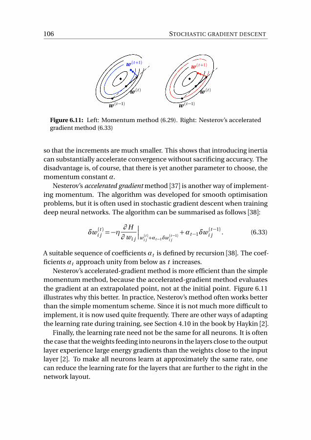
106 STOCHASTIC GRADIENT DESCENT
w (t−1)
w (t )
w (t+1)
w (t−1)
w (t )
w (t+1)
Figure 6.11: Left: Momentum method (6.29). Right: Nesterov’s acceleratedgradient method (6.33)
so that the increments are much smaller. This shows that introducing inertiacan substantially accelerate convergence without sacrificing accuracy. Thedisadvantage is, of course, that there is yet another parameter to choose, themomentum constant α.
Nesterov’s accelerated gradient method [37] is another way of implement-ing momentum. The algorithm was developed for smooth optimisationproblems, but it is often used in stochastic gradient descent when trainingdeep neural networks. The algorithm can be summarised as follows [38]:
δw (t )i j =−η
∂H
∂ wi j
�
�
�
w (t )i j +αt−1δw (t−1)i j
+αt−1δw (t−1)i j . (6.33)
A suitable sequence of coefficients αt is defined by recursion [38]. The coef-ficients αt approach unity from below as t increases.
Nesterov’s accelerated-gradient method is more efficient than the simplemomentum method, because the accelerated-gradient method evaluatesthe gradient at an extrapolated point, not at the initial point. Figure 6.11illustrates why this better. In practice, Nesterov’s method often works betterthan the simple momentum scheme. Since it is not much more difficult toimplement, it is now used quite frequently. There are other ways of adaptingthe learning rate during training, see Section 4.10 in the book by Haykin [2].
Finally, the learning rate need not be the same for all neurons. It is oftenthe case that the weights feeding into neurons in the layers close to the outputlayer experience large energy gradients than the weights close to the inputlayer [2]. To make all neurons learn at approximately the same rate, onecan reduce the learning rate for the layers that are further to the right in thenetwork layout.

RECIPES FOR IMPROVING THE PERFORMANCE 107
6.3.5 Pruning
The term pruning refers to removing unnecessary weights or neurons fromthe network, to improve its efficiency. The simplest approach is weightelimination by weight decay [39]. Weights that tend to remain very close tozero during training are removed by setting them to zero and not updatingthem anymore. Neurons that have zero weights for all incoming connectionsare effectively removed (pruned). It has been shown that this method canhelp the network to generalise [40].
An efficient pruning algorithm is based on the idea to remove the weightsthat have least effect upon the energy function (that minimise the increasein H upon removing them) [41]. Assume that the network was trained, sothat the network reached a (local) minimum of the energy function. Onestarts by expanding the energy function around this minimum. To write thisexpansion down in a convenient form, one groups all weights in the networkin a long weight vector w (as opposed to grouping them in a weight matrixW as we did in Chapter 2). A particular component wq is extracted from thevector w as follows:
wq = eq ·w q where eq =
...1...
← q . (6.34)
Here eq is the Cartesian unit vector in the direction q , with componentseq j =δq j . The expansion of H reads:
H =Hmin+12δw ·Mδw + higher orders in δw . (6.35)
The term linear in δw vanishes because we expand around a local minimum.The matrix M is the Hessian, the matrix of second derivatives of the energyfunction. Eliminating the weight δwq amounts to setting
δwq +wq = 0 . (6.36)
The idea is to minimise the damage to the network by eliminating the weightthat has least effect upon H
minq
minδw{ 1
2δw ·Mδw } subject to the constraint eq ·δw +wq = 0 . (6.37)

108 STOCHASTIC GRADIENT DESCENT
I omitted the constant term Hmin because it does not matter. Now we firstminimise H w.r.t. δw , for a given value of q . The linear constraint is incor-porated using a Lagrange multiplier as in Chapter 4, to form the Lagrangian
L = 12δw ·Mδw +λ(eq ·δw +wq ) . (6.38)
A necessary condition for a minimum (δw ,λ) satisfying the constraint is
∂L∂ δw
=Mδw +λeq = 0 and∂L∂ λ= eq ·δw +wq = 0 . (6.39)
We denote the solution of these Equations by δw ∗ and λ∗. It is obtained bysolving the linear system
�
M eq
eTq 0
��
δwλ
�
=
�
0−wq
�
. (6.40)
If M is invertible we can use a standard formula for the inversion of 2×2 blockmatrices to find the inverse of the matrix in Equation (6.40):
(eTq M−1eq )−1
�
M−1(eTq M−1eq )−M−1eq eTq M−1 M−1eq
eTq M−1 −1
�
. (6.41)
From Equations (6.40) and (6.41) we find that
δw ∗ =−M−1eq wq (eTq M−1eq )
−1and λ∗ =wq (eTq M−1eq )
−1 . (6.42)
The second step is to find the optimal q by minimising
L (δw ∗,λ∗; q ) =1
2w 2
q (eTq M−1eq )
−1 . (6.43)
The Hessian of the energy function is expensive to evaluate, and so is theinverse of this matrix. Usually one resorts to an approximate expression forM−1 [41]. One possibility is to set the off-diagonal elements of M to zero [42].
The algorithm is summarised in Algorithm 3. It turns out that this al-gorithm succeeds better than weight decay in reducing the unnecessaryweights in the network [41]. Weight decay eliminates the smallest weights.But small weights are often needed to achieve a small training error. Anotherpoint is that one obtains the weight elimination of the smallest weights bysubstituting M= I in the algorithm described above [Equation (6.43)]. Butthis is often not a good approximation.

SUMMARY 109
Algorithm 3 pruning least important weight
1: train the network to reach Hmin;2: compute M−1 approximately;3: determine q ∗ as the value of q for whichL (δw ∗,λ∗; q ) is minimal;4: if L (δw ∗,λ∗; q ∗)�Hmin then5: update all weights using δw =−wq ∗M−1eq ∗ (eTq ∗M
−1eq ∗ )−1;6: goto 2;7: else8: end;9: end if
6.4 Summary
Backpropagation is an efficient algorithm for stochastic gradient-descent onthe energy function in weight space, because it refers only to quantities thatare local to the weight to be updated. It is sometimes argued that biologicalneural networks are local in this way [2].
6.5 Further reading
The backpropagation algorithm is explained in Section 6.1. of Hertz, Kroghand Palmer [1], and in Chapter 4 of the book by Haykin [2]. The paper [36]by LeCun et al. predates deep learning, but it is still a very nice collection ofrecipes for making backpropagation more efficient. Historical note: one ofthe first papers on error backpropagation is the one by Rumelhart et al. [43].Have a look! The paper gives an excellent explanation and summary of thebackpropagation algorithm. The authors also describe results of differentnumerical experiments, one of them introduces convolutional nets (Section7.3) to learn to tell the difference between the letters T and C (Figure 6.12).
Figure 6.12: Patterns detected by the convolutional net of Ref. [43]. After Fig.13 in Ref. [43].

110 STOCHASTIC GRADIENT DESCENT
6.6 Exercises
Covariance matrix. Show that the covariance matrix C defined in Equation(6.19) is positive semidefinite.
Nesterov’s accelerated-gradient method. Show how the version (6.33) ofNesterov’s algorithm corresponds to the original formulation [37]. This pointis discussed in [38].
Pruning. Show that the expression (6.42) for the weight increment δw ∗ min-imises the Lagrangian (6.38) subject to the constraint.
Skipping layers. Show how the backpropagation algorithm can be gener-alised for feed-forward networks that allow for connections from the twonearest layers to the left, not only from the nearest layer to the left.
6.7 Exam questions
6.7.1 Multilayer perceptron
A classification problem is shown in Figure 6.13. Here, µ= 1,2, . . . ,11 is the
index of input pattern x (µ) = (x (µ)1 , x(µ)2 )
T, and t (µ) is the corresponding targetvalue.(a) Can this problem be solved by a simple perceptron with 2 input units,and a single output unit? Explain. (0.5p).(b) This problem can be solved by a multilayer perceptron with two input
units x(µ)i (i = 1,2), three hidden units V
(µ)j = θH
�
∑2i=1 w j k x
(µ)k −θ j
�
where
j = 1, 2, 3, and one output unit O (µ) = θH
�
∑3j=1 Wj V
(µ)j −Θ
�
. Here
θH (b ) =
¨
1 for b > 0 ,
0 for b ≤ 0(6.44)
is the Heaviside function, and w j k and Wj are weights for the hidden, andthe output layer, respectively. Finally, θ j and Θ are the thresholds assignedto the hidden units, and to the output unit. One way of solving the classifica-tion problem is illustrated in Fig. 6.13 where the three lines (solid, dashed,

EXAM QUESTIONS 111
and dash-dotted line) are determined by weights w j k and thresholds θ j as-signed to the three hidden units in the hidden layer. Compute w j k and θ j
corresponding to the lines shown in Fig. 6.13. Note that the point wherethe dashed and dash-dotted lines intersect has the following coordinates(0.5, 0.8)T. (0.5p).
(c) For each pattern x (µ)write its coordinates V(µ)
j in the transformed (hidden)space. (0.5p).(d) Graphically illustrate the problem in this transformed space. Is the prob-lem space linearly separable in the transformed space, or not? If yes, illustratea possible solution to the problem in this space. (0.5p)(e) Compute the corresponding weights Wj and the threshold Θ correspond-ing to the solution you illustrated in (d). (0.5p).
µ x(µ)1 x
(µ)2 t (µ)
1 0.1 0.95 02 0.2 0.85 03 0.2 0.9 04 0.3 0.75 15 0.4 0.65 16 0.4 0.75 17 0.6 0.45 08 0.8 0.25 09 0.1 0.65 1
10 0.2 0.75 111 0.7 0.2 1 0 0.2 0.4 0.6 0.8 1
0
0.1
0.2
0.3
0.4
0.5
0.6
0.7
0.8
0.9
1
x1
x2
Figure 6.13: Left: Inputs and target values for a classification problem. Thetarget output for each pattern µ is either t (µ) = 0 (white circles) or t (µ) = 1 (blackcircles). Right: the three lines illustrate a solution to the problem by a multilayerperceptron. Question 6.7.1.

112 STOCHASTIC GRADIENT DESCENT
6.7.2 Backpropagation
Explain how to train a multi-layer perceptron by back-propagation. Drawa flow-chart of the algorithm. In your discussion, refer to and explain thefollowing terms: forward propagation, backward propagation, hidden layer,energy function, gradient descent, local energy minima, batch mode, trainingset, validation set, classification error, and overfitting. Your answer must notbe longer than one A4 page. (1p).
6.7.3 Backpropagation
To train a multi-layer perceptron using backpropagation one needs updateformulae for the weights and thresholds in the network. Derive these updateformulae for the network shown in Fig. 6.14. The weights for the first and
second hidden layer, and for the output layer are denoted by w (1)j k , w (2)
m j , and
W1m . The corresponding thresholds are denoted by θ (1)j , θ (2)m , and Θ1, and
the activation function by g (· · · ). The target value for input pattern x (µ) is t(µ)1 .
The energy function is H = 12
∑
µ(t(µ)1 −O
(µ)1 )
2. (2p).
x(µ)k V
(1,µ)j V
(2,µ)m O
(µ)1
w (1)j k w (2)
m j
W1m
Figure 6.14: Multi-layer perceptron with three input terminals, two hiddenlayers, and one output unit. Question 6.7.3.

EXAM QUESTIONS 113
6.7.4 Backpropagation
A multilayer perceptron has L − 1 hidden layers (` = 1, . . . , L − 1 and one
output layer (l = L). The state of a neuron V(`,µ)
j in layer ` is given by
V(`,µ)
j = g (b (`,µ)j ) , with b(`,µ)j =−θ (`)j +
∑
k
w (`)j k V
(`−1,µ)k , (6.45)
where V (0,µ) equals the inputs x (µ) (V(0,µ)
k = x(µ)k ), w (`)
j k are weights, θ (`)j are
thresholds, and g (b ) is the activation function. The output is O(µ)j = g (b (L ,µ)
j ).
(a) Draw this network. Indicate where the elements x(µ)k , b
(`,µ)j , V
(`,µ)j , O
(µ)i ,
w (`)j k and θ (`)j for `= 1, . . . , L belong. (0.5 p)
(b) Derive the recursive rule for how the derivatives ∂ V(`,µ)
i /∂ w(p )mn depend
on the derivatives ∂ V(`−1,µ)
j /∂ w(p )mn for p < `. (1 p).
(c) Evaluate the derivative ∂ V(`,µ)
j /∂ w(p )mn for p = `. (0.5 p).
(d) Use gradient descent on the the energy function
H =1
2
∑
iµ
�
t(µ)i −O
(µ)i
�2, (6.46)
where t(µ)i is the target value for input pattern x (µ). Find the batch-mode
update rule for the weight w (L−2)mn with learning rate η. No momentum regu-
larisation. (1 p).
6.7.5 Backpropagation
To train a multi-layer perceptron with stochastic gradient descent one needsupdate formulae for the weights and thresholds in the network. Derivethese update formulae for the network shown in Fig. 6.15 using the gradient-descent algorithm with constant learning rate, no momentum and no weightdecay. The weights for the hidden layer and for the output layer are denotedby w j k and W1 j , respectively. The corresponding thresholds are denoted byθ j , and Θ1, and the activation function by g (· · · ). The target value for input
pattern x (µ) is t(µ)1 , and the network output is O
(µ)1 . The energy function is
H = 12
∑pµ=1
�
t(µ)1 −O
(µ)1
�2. (2p)

114 STOCHASTIC GRADIENT DESCENT
x(µ)k V
(µ)j O
(µ)1
w j k W1 j
Figure 6.15: Multi-layer perceptron. Question 6.7.5.
6.7.6 True/false questions
Indicate wether the following statements are true or false. 13 correct answersgive 1.5 points, 12 correct answers give 1.0 point and 10-11 correct answersgive 0.5 points and 0-9 correct answers give zero points. (1.5 p).
1. Backpropagation is a form of unsupervised learning.2. For backpropagation to work the weights must be symmetric.3. For backpropagation it is necessary to know the target outputs of input
patterns in the training set.4. Early stopping in backpropagation is a way to avoid overfitting.5. Early stopping in backpropagation helps to avoid getting stuck in local
minima of energy.6. The randomness in stochastic gradient descent helps to avoid being
stuck in local minima of energy.7. The randomness in stochastic gradient descent prevents overfitting.8. There are 2(2
n ) Boolean functions with n inputs.9. None of the Boolean functions with 5 inputs are linearly separable.
10. There are 24 Boolean functions with three input units (and output 0/1)where exactly three input patterns map to 0.
11. When solving a t =±1-problem in two dimensions using a decisionboundary, the resulting output problem may sometimes not be linearlyseparable.
12. The training time for stochastic gradient descent may depend on howthe weights are initialised.
13. The number of neurons in the input layer of a perceptron is equal tothe number of input patterns.

115
Figure 7.1: Images of iris flowers. From left to right: iris setosa (copyright T.Monto), iris versicolor (copyright R. A. Nonemacher), and iris virginica (copy-right A. Westermoreland). All images are copyrighted under the creative com-mons license.
7 Deep learning
7.1 How many hidden layers?
In Chapter 5 we saw why it is sometimes necessary to have a hidden layer:this make it possible to solve problems that are not linearly separable. Underwhich circumstances is one hidden layer sufficient? Are there problems thatrequire more than one hidden layer? Even if not necessary, may additionalhidden layers improve the performance of the network?
The second question is more difficult to answer than the first, so we startwith the first question. To understand how many hidden layers are necessaryit is useful to view the classification problem as an approximation problem[44]. Consider the classification problem (x (µ), t (µ)) for µ = 1, . . . , p . Thisproblem defines a target function t (x ). Training a network to solve this task
g (b ) = bg (b ) =σ(b )
xkV (1)l
V (2)j
O (x )Wj
w (2)j l
w (1)l k
Figure 7.2: Multi-layer perceptron for function approximation.

116 DEEP LEARNING
x
t (x ) O (x )
Figure 7.3: The neural-network output O (x ) approximates the target functiont (x ).
corresponds to approximating the target function t (x ) by the output functionO (x ) of the network, from N -dimensional input space to one-dimensionaloutput space.
How many hidden layers are necessary or sufficient to approximate agiven set of functions to a certain accuracy, by choosing weights and thresh-olds? The answer depends on the nature of the set of functions. Are theyreal-valued or do they assume only discrete values? If the functions arereal-valued, are they continuous or not?
We start by considering real-valued inputs and output. Consider the net-work drawn in Figure 7.2. The neurons in the hidden layers have sigmoidactivation functionsσ(b ) = (1+e−b )−1. The output is continuous, with acti-vation function g (b ) = b . With two hidden layers the task is to approximatethe function t (x ) by
O (x ) =∑
j
Wj g
�
∑
l
w (2)j l g
�∑
k
w (1)l k xk −θ
(1)l
�
−θ (2)j
�
−Θ . (7.1)
In the simplest case the inputs are one-dimensional (Figure 7.3). Thetraining set consists of pairs (x (µ), t (µ)). The task is then to approximate thecorresponding target function t (x ) by the network output O (x ):
O (x )≈ t (x ) . (7.2)
We approximate the real-valued function t (x ) by linear combinations ofthe basis functions b (x ) shown in Figure 7.4(a). Any reasonable real-valuedfunction t (x ) can be approximated by a sums of such basis functions, each

HOW MANY HIDDEN LAYERS? 117
b (x )
x
σ�
a1(x − c1)�
−σ�
a2(x − c2)�
xc1 c2
Figure 7.4: (a) basis function. (b) linear combination of two sigmoid functionsfor a large value of a1 = a2.
suitably shifted and scaled. Furthermore, these basis functions can be ex-pressed as differences of activation functions [Figure 7.4(b)]
b (x ) =σ(w1 x −θ1)−σ(w2 x −θ2) . (7.3)
Comparison with Equation (7.1) shows that one hidden layer is sufficient toconstruct the function O (x ) in this way.
Now consider two-dimensional inputs. In this case, suitable basis func-tions are
σ [σ(x1)−σ(x1−θ1) +σ(x2)−σ(x2−θ2)−θ ] . (7.4)
So for two input dimensions two hidden layers are sufficient, with four neu-rons in the first layer, and one neuron per basis function in the second hiddenlayer. In general, for N inputs, two hidden layers are sufficient, with 2N unitsin the first layer, and one unit per basis function in second layer.
Yet it is not always necessary to use two layers for real-valued functions.For continuous functions, one hidden layer is sufficient. This is ensured bythe universal approximation theorem [2]. This theorem says any continuousfunction can be approximated to arbitrary accuracy by a network with asingle hidden layer, for sufficiently many neurons in the hidden layer.
In Chapter 5 we considered discrete Boolean functions. It turns out thatany Boolean function with N -dimensional inputs can be represented by anetwork with one hidden layer, using 2N neurons in the hidden layer:
xk ∈ {+1,−1} k = 1, . . . , N inputs
Vj j = 0, . . . , 2N −1 hidden neurons
g (b ) = tanh(b ) activation function of hidden neurons (7.5)
g (b ) = sgn(b ) activation function of output unit

118 DEEP LEARNING
x1 x2 t
-1 -1 -1
+1 -1 +1
-1 +1 +1
+1 +1 -1
k = 2
k = 1
0
1
2
3xk w j k
Vj
W1 j
O1
(a) (b) (c)
j digit 1 digit 2
0 0 0
1 0 1
2 1 0
3 1 1
Figure 7.5: Boolean XOR function. (a) value table, (b) network layout. Forthe weights feeding into the hidden layer, dashed lines correspond to w j k =−δ , solid lines to w j k = δ. For the weights feeding into the output neuron,dashed lines correspond to W1 j =−γ, and solid lines to W1 j = γ (b) constructionprinciple for the weights of the hidden layer.
A difference compared with the Boolean networks in Section 5.4 is that herethe inputs take the values ±1. The reason is that this simplifies the proof.
This proof goes by construction [1]. For each hidden neuron one assignsthe weights as follows
w j k =
¨
δ if the k thdigit of binary representation of j is 1 ,
−δ otherwise,(7.6)
with δ > 1 (see below). The thresholds θ j of all hidden neurons are the same,equal to N (δ−1). The idea is that each input pattern turns on exactly oneneuron in the hidden layer (called the winning unit). This requires that δ islarge enough, as we shall see. The weights feeding into the output neuronare assigned as follows. If the output for the pattern represented by neuronVj is +1, let W1 j = γ> 0, otherwise W1 j =−γ. The threshold is Θ =
∑
j W1 j .
To show how this construction works, consider the Boolean XOR functionas an example. First, for each pattern only the corresponding winning neurongives a positive signal. For pattern x (1) = [−1,−1]T, for example, this is thefirst neuron in the hidden layer ( j = 0). To see this, compute the local fields

HOW MANY HIDDEN LAYERS? 119
for this input pattern:
b (1)0 = 2δ−2(δ−1) = 2 , (7.7)
b (1)1 = −2(δ−1) = 2−2δ ,
b (1)2 = −2(δ−1) = 2−2δ ,
b (1)3 = −2δ−2(δ−1) = 2−4δ .
If we choose δ > 1 then the output of the first hidden neuron gives a positiveoutput (V0 > 0), the other neurons produce negative outputs, Vj < 0 forj = 1, 2, 3. Now consider x (3) = [−1,+1]T. In this case
b (3)0 = −2(δ−1) = 2−2δ (7.8)
b (3)1 = −2δ−2(δ−1) = 2−4δ
b (3)2 = 2δ−2(δ−1) = 2
b (3)3 = −2(δ−1) = 2−2δ
So in this case the third hidden neuron gives a positive output, while theothers yield negative outputs. It works in the same way for the other twopatterns, x (2) and x (4). This confirms that there is a unique winning neuronfor each pattern. That pattern µ= k gives the winning neuron j = k −1 is ofno importance, it is just a consequence of how the patterns are ordered inthe value table in 7.5. Second, the output neuron computes
O1 = sgn(−γV1+γV2+γV3−γV4) (7.9)
with γ > 0, and Θ =∑
j W1 j = 0. For x (1) and x (4) we find the correct result
O1 =−1. The same is true for x (2) and x (3), we obtain O1 = 1. In summary, thisexample illustrates how an N -dimensional Boolean function is representedby a network with one hidden layer, with 2N neurons. The problem is ofcourse that this network is expensive to train for large N because the numberof hidden neurons is very large.
There are more efficient layouts if one uses more than one hidden layer.As an example, consider the parity function for N binary inputs equal to 0 or1. The function measures the parity of the input sequence. It gives 1 if thereis an odd number of ones in the input, otherwise 0. A construction similar tothe above yields a network layout with 2N neurons in the hidden layer. If one

120 DEEP LEARNING
1
11
11
11
1
1
00
0
0
00
0
0
0
0
0
1
0
0
0
0
0
1
0
0
1
1
Figure 7.6: Solution of the parity problem for N -dimensional inputs. Thenetwork is built from XOR units (Figure 5.14). Each XOR unit has a hidden layerwith two neurons. Above only the states of the inputs and outputs of the XORunits are shown, not those of the hidden neurons. In total, the whole networkhas O (N ) neurons.
instead wires together the XOR networks shown in Figure 5.14, one can solvethe parity problem with O (N ) neurons, as Figure 7.6 demonstrates. WhenN is a power of two then this network has 3(N −1) neurons. To see this, setthe number of inputs to N = 2k . Figure 7.6 shows that the numberNk ofneurons satisfies the recursionNk+1 = 2Nk +3 withN1 = 3. The solution ofthis recursion isNk = 3(2k −1).
This example also illustrates a second reason why it may be useful tohave more than one hidden layer. To design a network for a certain task itis often convenient to build the network from building blocks. One wiresthem together, often in a hierarchical fashion. In Figure 7.6 there is only onebuilding block, the XOR network from Figure 5.14.
Another example are convolutional networks for image analysis (Section7.3). Here the fundamental building blocks are feature maps, they recognisedifferent geometrical features in the image, such as edges or corners.

TRAINING DEEP NETWORKS 121
input `= 1 `= 2 `= 3 `= 4 `= 5 output
Figure 7.7: Fully connected deep network with five hidden layers. How deepis deep? Usually one says: deep networks have two or more hidden layers.
7.2 Training deep networks
It was believed for a long time that networks with many hidden layers (deepnetworks) are so difficult to train that it is not practical to use many hiddenlayers. But the past few years have witnessed a paradigm shift regarding thisquestion. It has been demonstrated that fully connected deep networks canin fact be trained efficiently with backpropagation (Section 6.2), and thatthese networks can solve complex classification tasks with very small errorrates.
Browsing through the recent literature of the subject one may get theimpression that training deep networks such as the one shown in Figure 7.7is more an art than a science, some read like manuals, or like collectionsof engineering recipes. But there are several fundamental facts about howdeep networks learn. I summarise them in this Section. A comprehensivesummary of these (and more) principles is given in the book Deep learning[4].
7.2.1 Unstable gradients
In Chapter 6 we discussed that the learning slows down when the gradientsg ′(b )become small. When the network has many hidden layers, this problembecomes worse. One finds that the neurons in hidden layers close to theinput layer (small values of ` in Figure 7.7) change only by small amounts,the smaller the more hidden layers the network has. One way of quantifyingthis effect is to measure the gradient of the energy function with respect to

122 DEEP LEARNING
0 10 20 30 40 5010-1
100
101
102
epochs
|∇(`)θ
H|
Figure 7.8: Shows how the norm of the gradient of H w.r.t. θ (`)j in layer `depends on the number of training epochs. Gradient in hidden layer `= 1 (◦),`= 2 (�), `= 3 (◊), `= 4 (4). The data was obtained by training a network withfour fully connected hidden layers with N = 30 neurons each on the MNISTdata set (Section 7.4). The output layer has 10 neurons. Sigmoid activationfunctions (6.15a), quadratic energy function (6.4), learning rate η = 3× 10⁻³.The data was obtained by averaging over an ensemble of 100 independent runs(data by Johan Fries).
the thresholds in layer `
∇(`)θ H =
∂
∂ θ (`)1...∂
∂ θ (`)N
H . (7.10)
Equation (6.12) shows that the errors in layer ` and thus the weight updates
are proportional to −∇(`)θ H . Figure 7.8 demonstrates that the norm of thisgradient tends to be very small for the first 20 training epochs. In this regimethe gradient (and thus the speed of training) vanishes exponentially as `→ 1.This slowing down is the result of the diminished effect of the neurons in layer` upon the output, when ` is small. This is the vanishing-gradient problem.
To explain this phenomenon, consider the very simple case shown inFigure 7.9: a deep network with only one neuron per layer. To measure theeffect of a given neuron on the output, we calculate how the output of thenetwork changes when changing the state of a neuron in a particular layer.

TRAINING DEEP NETWORKS 123
θ (1) θ (2) θ (L−1) θ (L )w (1) w (2) w (3) w (L−1) w (L )
x V (1) V (2) V (L−1) V (L )
Figure 7.9: ‘Network’ illustrating the vanishing-gradient problem, with neu-rons V (`), weights w (`), and thresholds θ (`).
The output V (L ) is given by the nested activation functions
V (L )=g�
w (L )g�
w (L−1) · · ·g�
w (2)g (w (1)x−θ (1))−θ (2)�
. . .−θ (L−1)�
−θ (L )�
. (7.11)
The effects of the neurons in Figure 7.9 are computed using the chain rule:
∂ V (L )
∂ V (L−1)= g ′(b (L ))w (L )
∂ V (L )
∂ V (L−2)=
∂ V (L )
∂ V (L−1)
∂ V (L−1)
∂ V (L−2)= g ′(b (L ))w (L )g ′(b (L−1))w (L−1)
... (7.12)
where b (k ) =w (k )V (k−1)−θ (k ) is the local field for neuron k . This yields thefollowing expression for J`,L ≡ ∂ V (L )/∂ V (`):
J`,L =∂ V (L )
∂ V (`)=`+1∏
k=L
[g ′(b (k ))w (k )] . (7.13)
Note that the errorδ(`) of the hidden layer ` is determined by a closely relatedproduct. Algorithm 2 shows that the errors are given recursively by δ(`) =δ(`+1)w (`+1)g ′(b (`)). Using δ(L ) = [t −V (L )(x )]g ′(b (L ))we have
δ(`) = [t −V (L )(x )]g ′(b (L ))`+1∏
k=L
[w (k )g ′(b (k−1))] . (7.14)
Equations (7.13) and (7.14) are consistent sinceδ(`)=[t −V (L )]∂ V (L )/∂ (−θ (`))= [t −V (L )]∂ V (L )/∂ V (`)g ′(b (`)).
Coming back to the product (7.13), consider first the early stages of train-ing. If one initialises the weights as described in Chapter 6 to Gaussian

124 DEEP LEARNING
random variables with mean zero and variance σ2w , and the thresholds to
zero, then the factors w (k )g ′(b (k−1)) are usually smaller than unity (for theactivation functions (6.15), the maximum of g ′(b ) is 1
2 and 1, respectively).The product of these factors vanishes quickly as ` decreases. So the slowingdown is a consequence of multiplying many small numbers to get somethingreally small (vanishing-gradient problem).
What happens at later times? One might argue that the weights may growduring training, as a function of `. If that happened, the problem might be-come worse still, because g ′(b ) tends to zero exponentially as |b | grows. Thisindicates that the first layers may continue to learn slowly. Figure 7.8 showsthat the effect persists for about 20 epochs. But then even the first layersbegin to learn faster. This does not contradict the above discussion, becauseit assumed random weights. As the network learns, the weights are no longerindependent random numbers. But there is to date no mathematical theorydescribing how this transition occurs.
More fundamentally, Equation (7.13) demonstrates that different layersof the network learn at different speeds, because their neurons typically havedifferent effects on the output. This is due to the fact that the product inEquation (7.13) is unlikely to remain of order unity when L is large. To see this,assume that the weights are independently distributed random numbers.Taking the logarithm and using the central-limit theorem shows that thedistribution of the product is log normal. This means that the learning speedcan be substantially different in different layers. This is also referred to theproblem of unstable gradients. The example shown in Figure 7.9 illustratesthe origin of this problem: it is due to the fact that multiplying many smallnumbers together produces a result that is very small. Multiplying manynumbers that are larger than unity, by contrast, yields a large result.
In networks like the one shown in Figure 7.7 the principle is the same, butinstead of multiplying numbers one multiplies matrices. The product (7.13)of random numbers becomes of product of random matrices. Assume thatall layers `= 1, . . . , L have N neurons. We denote the matrix with elements
J (`,L )i j = ∂ V (L )i /∂ V (`)j by J`,L . Using the chain rule we find:
∂ V (L )i
∂ V (`)j
=∑
l m ···n
∂ V (L )i
∂ V (L−1)l
∂ V (L−1)l
∂ V (L−2)m
· · ·∂ V (`+1)
n
∂ V (`)j
. (7.15)

TRAINING DEEP NETWORKS 125
Using the update rule
V (k )i = g�∑
j
w (k )i j V (k−1)
j −θ (k )i
�
(7.16)
we can evaluate each factor:
∂ V (k )p
∂ V (k−1)l
= g ′(b (k )p )w(k )p l . (7.17)
In summary, this yields the following expression for J`,L :
J`,L =D(L )W(L )D(L−1)W(L−1) · · ·D(`+1)W(`+1) , (7.18)
where W(k ) is the matrix of weights feeding into layer k , and
D(k ) =
g ′(b (k )1 )...
g ′(b (k )N )
. (7.19)
This expression is analogous to Equation (7.13).The eigenvalues of the matrix J0,k describe how small changesδV (0) to the
inputs V (0) (or small differences between the inputs) grow as they propagatethrough the layers. If the maximal eigenvalue is larger than unity, then |δV (0)|grows exponentially as a function of layer index k . This is quantified by themaximal Lyapunov exponent [45]
λ= limk→∞
1
2k
log tr�
JT0,k J0,k
��
(7.20)
where the average is over realisations of weights and thresholds. The matrixJT
0,k J0,k is called the right Cauchy-Green matrix, and tr denotes the traceof this matrix, the sum of its diagonal elements. The right Cauchy-Greenmatrix is symmetric, and it is positive definite. The eigenvectors of JT
0,k J0,k
are called forward Lyapunov vectors. They describe how small corrections tothe inputs rotate, shrink, or stretch as they propagate through the network.
If we multiply the matrix Jk ,L from the left with the transpose of thevector δ(L ) of output errors, we see how the errors change as they propagatebackwards from layer k to the leftmost hidden layer, how this vector rotates,shrinks, or stretches.

126 DEEP LEARNING
(a) (b)f (I )
I2 4 6 8 10
0.050.1
max{0, b }
b
Figure 7.10: (a) Firing rate of a leaky integrate-and-fire neuron as a function ofthe electrical current I through the cell membrane, Equation (7.22) for τ= 25and Uc/R = 2 (see text). (b) Rectified linear unit, g (b ) =max{0, b }.
There are a number of different tricks that help to suppress vanishinggradients, to some extent at least. First, it is usually argued that it helpsto use an activation function that does not saturate at large b , such as theReLU function introduced in Section 7.2.2. But the results of Ref. [46] showthat the effect is perhaps not as strong as originally thought. Second, batchnormalisation (Section 7.2.6) may help against the unstable gradient problem.Third, introducing connections that skip layers (residual network) can alsoreduce the unstable-gradient problem. This is discussed in Section 7.6.
7.2.2 Rectified linear units
Glorot et al. [47] suggested to use a different activation function. Theirchoice is motivated by the response curve of leaky integrate-and-fire neurons.This is a model for the relation between the electrical current I through thecell membrane into the neuron cell, and the membrane potential U . Thesimplest models for the dynamics of the membrane potential represent theneuron as a capacitor. In the leaky integrate-and-fire neuron, leakage isadded by a resistor R in parallel with the capacitor C , so that
I =U
R+C
dU
dt. (7.21)
For a constant current, the membrane potential grows from zero as a functionof time, U (t ) =R I [1−exp(−t /τ)], where τ=R C is the time constant of themodel. One says that the neuron produces a spike when the membranepotential exceeds a critical value, Uc. Immediately after, the membranepotential is set to zero (and begins to grow again). In this model, the firingrate f (I ) is thus given by t −1
c , where tc is the solution of U (t ) =Uc. It followsthat the firing rate exhibits a threshold behaviour (the system works like a

TRAINING DEEP NETWORKS 127
rectifier):
f (I ) =
¨
0 for I ≤Uc/R ,�
τ log�
R IR I−Uc
��−1for I >Uc/R .
(7.22)
This response curve is illustrated in Figure 7.10 (a). The main message is thatthere is a threshold below which the response is strictly zero (this is not thecase for the activation function shown in Figure 1.6). The response functionlooks qualitatively like the ReLU function
g (b ) =ReLU(b )≡max{0, b } , (7.23)
shown in panel (b). Neurons with this activation function are called rectifiedlinear units. The derivative of the ReLU function is discontinuous at b = 0. Acommon convention is to set the derivative to zero at b = 0.
What is the point of using rectified linear units? When training a deepnetwork with ReLU functions it turns out that many of the hidden neurons(as many as 50%) produce outputs strictly equal to zero. This means thatthe network of active neurons (non-zero output) is sparsely connected. It isthought that sparse networks have desirable properties, and sparse repre-sentations of a classification problem are more likely to be linearly separable(as shown in Section 10.1). Figure 7.11 illustrates that for a given input pat-tern only a certain fraction of hidden neurons is active. For these neuronsthe computation is linear, yet different input patterns give different sets ofactive neurons. The product in Equation (7.18) acquires a particularly sim-ple structure: the matrices D(k ) are diagonal with 0/1 entries. But while theweight matrices are independent, the D(k )-matrices are correlated: whichelements vanish depends on the states of the neurons in the correspondinglayer, which in turn depend on the weights to the right of D(k ) in the matrixproduct.
A hidden layer with only one or very few active neurons might act as abottleneck preventing efficient backpropagation of output errors which couldin principle slow down training. For the examples given in Ref. [47] this doesnot occur.
The ReLU function is unbounded for large positive local fields. Therefore,the vanishing-gradient problem (Section 7.2.1) is thought to be less severein networks made of rectified linear units, but see Ref. [46]. Since the ReLUfunction does not saturate, the weights tend to increase. Glorot et al. [47]

128 DEEP LEARNING
input `= 1 `= 2 `= 3 `= 4 `= 5 output
Figure 7.11: Sparse network of active neurons with ReLU activation functions.The red paths correspond to active neurons with positive local fields.
suggested to use L1-weight decay (Section 6.3.3) to make sure that the weightsdo not grow.
Finally, using ReLU functions instead of sigmoid functions speeds up thetraining, because the ReLU function has piecewise constant derivatives. Suchfunction calls are faster to evaluate than sigmoid functions, for example.
7.2.3 Outputs and cost functions
Up to now we discussed networks that have the same activation functions forall neurons in all layers, either sigmoid or tanh activation functions (Equa-tion 6.15), or ReLU functions (Section 7.2.2). These networks are trainedby stochastic gradient descent on the quadratic energy function (5.25). Ithas been shown that it may be advantageous to employ a different energyfunction, and to use slightly different activation functions for the neurons inthe output layer, so-called softmax outputs, defined as
Oi =eαb (L )i
∑Mk=1 eαb (L )k
. (7.24)
Here b (L )i =∑
j w (L )i j V (L−1)
j −θ (L )i are the local fields in the output layer. Usuallythe constant α is taken to be unity. In the limit α→∞, you see that Oi =δi i0
where i0 is the index of the winning output unit, the one with the largest
value b (L )i (Chapter 9). Usually one takes α= 1, then Equation (7.24) is a softversion of this maximum criterion, thus the name softmax. Three importantproperties of softmax outputs are, first, that 0≤Oi ≤ 1. Second, the values of

TRAINING DEEP NETWORKS 129
the outputs sum to oneM∑
i=1
Oi = 1 . (7.25)
This means that the outputs of softmax units can be interpreted as proba-bilities. Third, the outputs are monotonous: when b (L )i increases then Oi
increases but the values Ok of the other output neurons k 6= i decrease.Softmax output units can simplify interpreting the network output for
classification problems where the inputs must be assigned to one of M
classes. In this problem, the output O(µ)i of softmax unit i represents the
probability that the input x (µ) is in class i (in terms of the targets: t(µ)i = 1
while t(µ)k = 0 for k 6= i ). Softmax units are often used in conjunction with a
different energy function (or cost function). It is defined in terms of negativelog likelihoods
H =−∑
iµ
t(µ)i log O
(µ)i . (7.26)
Here and in the following log stands for the natural logarithm. The function
(7.26) is minimal when O(µ)i = t
(µ)i . Since the function (7.26) is different from
the energy function used in Chapter 6, the details of the backpropagationalgorithm are slightly different. To find the correct formula for backpropaga-tion, we need to evaluate
∂H
∂ wmn=−
∑
iµ
t(µ)i
O(µ)i
∂ O(µ)i
∂ wmn. (7.27)
Here I did not write out the labels L that denote the output layer, and in thefollowing equations I also drop the index µ that refers to the input pattern.Using the identities
∂ Oi
∂ bl=Oi (δi l −Ol ) and
∂ bl
∂ wmn=δl m Vn , (7.28)
one obtains
∂ Oi
∂ wmn=∑
l
∂ Oi
∂ bl
∂ bl
∂ wmn=Oi (δi m −Om )Vn . (7.29)

130 DEEP LEARNING
O1
O2...
OM−1
OM
soft
max
Figure 7.12: The symbol for a softmax layer indicates that the neurons in thislayer are not independent.
So
δwmn =−η∂H
∂ wmn=η
∑
iµ
t(µ)i (δi m−O (µ)m )V
(µ)n =η
∑
µ
(t (µ)m −O (µ)m )V(µ)
n , (7.30)
since∑M
i=1 t(µ)i = 1 for the type of classification problem where each input be-
longs to precisely one class. The corresponding expression for the thresholdupdates reads
δθm =−η∂H
∂ θm=−η
∑
µ
(t (µ)m −O (µ)m ) . (7.31)
Equations (7.30) and (7.31) highlight a further advantage of softmax outputneurons (apart from the fact that they allow the output to be interpreted interms of probabilities). The weight and threshold increments for the outputlayer derived in Section 6 [Equations (6.7) and (6.12a)] contain factors of
derivatives g ′(B (µ)m ). As noted earlier, these derivatives tend to zero whenthe activation function saturates, slowing down the learning. But Equations(7.30) and (7.31) do not contain such factors! Here the rate at which theneuron learns is simply proportional to the error, (t (µ)m −O
(µ)m ), no small factors
reduce this rate.Softmax units are normally only used in the output layer. First, the deriva-
tion shows that the learning speedup mentioned above is coupled to theuse of the log likelihood function (7.26). Second, one usually tries to avoiddependence between the neurons in a given hidden layer, but Equation(7.24) shows that the output of neuron i depends on all local fields in thehidden layer (Figure 7.12). A better alternative is usually the ReLU activationfunction discussed in Section 7.2.2.
There is an alternative way of choosing the cost function that is very

TRAINING DEEP NETWORKS 131
similar to the above, but works with sigmoid units:
H =−∑
iµ
t(µ)i log O
(µ)i + (1− t
(µ)i ) log(1−O
(µ)i ) , (7.32)
with Oi =σ(bi )whereσ is the sigmoid function (6.15a). The function (7.32)is called cross-entropy function. To compute the weight increments, we applythe chain rule:
∂H
∂ wmn=∑
iµ
�
t(µ)i
O(µ)i
−1− t
(µ)i
1−O(µ)i
�
∂ Ol
∂ wmn=∑
iµ
t(µ)i −O
(µ)i
O(µ)i (1−O
(µ)i )
∂ Ol
∂ wmn. (7.33)
Using Equation (6.16a) we obtain
δwmn =η∑
µ
(t (µ)m −O (µ)m )V(µ)
n , (7.34)
identical to Equation (7.30). The threshold increments are also updated inthe same way, Equation (7.31). Yet the interpretation of the outputs is slightlydifferent, since the values of the softmax units in the output layers sum tounity, while those of the sigmoid units do not. In either case you can use thedefinition (6.23) for the classification error.
7.2.4 Weight initialisation
The results of Section 7.2.1 point to the importance of initialising the weightsin the right way, to avoid that the learning slows down. This is significantbecause it is often found that the initial transient learning phase poses asubstantial bottleneck to learning [48]. For this initial transient, correctweight initialisation can give a substantial improvement.
Moreover, when training deep networks with sigmoid activation functionsin the hidden layers, it was observed that the values of the output neuronsremain very close to zero for many training iterations (Figure 2 in Ref. [49]),slowing down the training substantially. It is argued that this is a consequenceof the way the weights are initialised, in combination with the particularshape of the sigmoid activation function. It is sometimes argued that tanhactivation functions work better than sigmoids, although the reasons are notquite clear.

132 DEEP LEARNING
So, how should the weights be initialised? The standard choice is to ini-tialise the weights to independent Gaussian random numbers with meanzero and unit variance and the thresholds to zero (Section 6.1). But in net-works that have large hidden layers with many neurons, this scheme may fail.Consider a neuron i in the first hidden layer with N incoming connections.Its local field
bi =N∑
j=1
wi j x j (7.35)
is a sum of many independently identically distributed random numbers.Assume that the input patterns have independent random bits, equal to0 or 1 with probability 1
2 . From the central-limit theorem we find that thelocal field is Gaussian distributed in the limit of large N , with mean zero andvariance
σ2b =σ
2w N /2 . (7.36)
This means that the local field is typically quite large, of orderp
N , and thisimplies that the units of the first hidden layer saturate – slowing down thelearning. This conclusion rests on our particular assumption concerningthe input patterns, but it is in general much better to initialise the weightsuniformly or Gaussian with mean zero and with variance
σ2w ∝N −1 , (7.37)
to cancel the factor of N in Equation (7.36). The thresholds can be initialisedto zero, as described in Section 6.1.
The normalisation (7.37) makes sure that the weights are not too large ini-tially, but it does not circumvent the vanishing-gradient problem discussedin Section 7.2.1. There the problem was illustrated for N = 1, so unit variancefor the initial weight distribution corresponds to Equation (7.37).
7.2.5 Regularisation
Deeper networks have more neurons, so the problem of overfitting (Figure6.9) tends to be more severe for deeper networks. Therefore regularisationschemes that limit the tendency to overfit are more important for deepernetworks. In Section 6.3.3 several regularisation schemes were described, forexample L1- and L2-regularisation. In training deep networks, a number of

TRAINING DEEP NETWORKS 133
Figure 7.13: Illustrates regularisation by drop out.
other regularisation schemes have proved useful: drop out, pruning (Section6.3.5), and expanding the training set.
Drop out
In this scheme some neurons are ignored during training [50]. Usually thisregularisation technique is applied to hidden neurons. The procedure isillustrated in Figure 7.13. In each step of the training algorithm (for eachmini batch, or for each individual pattern) one ignores at random a fraction pof neurons from each hidden layer, and updates the weights in the remaining,diluted network in the usual fashion. The weights coming into the droppedneurons are not updated, and as a consequence neither are their outputs. Forthe next step in the training algorithm, the removed neurons at put back, andanother set of hidden neurons is removed. Once the training is completed,all hidden neurons are activated, but their outputs are multiplied by p .
Srivastava et al. [50]motivate this method by remarking that the perfor-mance of machine-learning algorithms is usually improved by combiningthe results of several learning attempts. In our case this corresponds to sep-arately training several networks with different layouts on different inputs,and then to average over their outputs. However, for deep networks this iscomputationally very expensive. Drop out is an attempt to achieve the samegoal more efficiently. The idea is that dropout corresponds to effectivelytraining a large number of different networks. If there are k hidden neurons,then there are 2k different combinations of neurons that are turned on oroff. The hope is that the network learns more robust features of the inputdata in this way, and that this reduces overfitting. In practice the methodis usually applied together with another regularisation scheme, max-norm

134 DEEP LEARNING
n 10 8 6 4 2
Training success
without pruning 98.5 96.8 92.5 78.3 49.1
pruned network - - - 97.9 83.3
Figure 7.14: Boolean XOR problem. The network has one hidden layer with nReLU neurons. The output neuron has a sigmoid activation function. The net-work is trained with stochastic gradient descent for 10 000 iterations. The initialweights were Gaussian random numbers with mean zero, standard deviation0.1, and max-norm regularisation |wi j |< 2. The thresholds were initially zero.Training success was measured in an ensemble of 1000 independent trainingrealisations. Data from Ref. [51].
regularisation. This simply means that weights are not allowed to grow largerthan a given constant: |wi j | ≤ c .
Pruning
Pruning (Section 6.3.5) is also a regularisation method: by removing unnec-essary weights one reduces the risk of overfitting. As opposed to drop out,where hidden neurons are only temporarily ignored, pruning refers to per-manently removing hidden neurons. The idea is to train a large network, andthen to prune a large fraction of neurons to obtain a much smaller network.It is usually found that such pruned nets generalise much better than smallnets that were trained without pruning. Up to 90% of the hidden neurons canbe removed. This method is applied with success to deep networks, but hereI want to discuss a simple example: Frankle & Carbin [51] used the BooleanXOR function to illustrate the effectiveness of pruning.
Figure 5.14 shows that the XOR function can be represented by a hiddenlayer with two neurons. Suitable weights and thresholds are given in thisFigure. Frankle & Carbin [51] point out that backpropagation takes a longtime to find a valid solution, for random initial weights. They observe thata network with many more neurons in the hidden layer usually learns bet-ter. Figure 7.14 lists the fraction of successful trainings for networks with

TRAINING DEEP NETWORKS 135
different numbers of neurons in the hidden layer. With two hidden neu-rons, only 49.1% of the networks learned the task in 10 000 training steps ofstochastic gradient descent. Networks with more neurons in the hidden layerensure better training success. The Figure also shows the training successof pruned networks, that were initially trained with n = 10 neurons. Thennetworks were pruned iteratively during training, removing the neurons withthe largest average magnitude. After training, the weights and thresholdwere reset to their initial values, the values before training began. One candraw three conclusions from this data (from Ref. [51]). First, iterative prun-ing during training singles out neurons in the hidden layer that had initialweights and thresholds resulting in the correct decision boundaries. Sec-ond, the pruned network with two hidden neurons has much better trainingsuccess than the network that was trained with only two hidden neurons.Third, despite pruning more than 50% of the hidden neurons, the networkwith n = 4 hidden neurons performs almost as well as then one with n = 10hidden neurons. When training deep networks it is common to start withmany neurons in the hidden layers, and to prune up to 90% of them. Thisresults in small trained networks that can efficiently and reliably classify.
Expanding the training set
If one trains a network with a fixed number of hidden neurons on largertraining sets, one observes that the network generalises with higher accuracy(better classification success). The reason is that overfitting is reduced whenthe training set is larger. Thus, a way of avoiding overfitting is to expandor augment the training set. It is sometimes argued that the recent successof deep neural networks in image recognition and object recognition is inlarge part due to larger training sets. One example is ImageNet, a databaseof more than 107 hand-classified images, into more than 20 000 categories[52]. Naturally it is expensive to improve training sets in this way. Instead,one can expand a training set artificially. For digit recognition (Figure 2.1),for example, one can expand the training set by randomly shifting, rotating,and shearing the digits.

136 DEEP LEARNING
7.2.6 Batch normalisation
Batch normalisation [53] can significantly speed up the training of deepnetworks with backpropagation. The idea is to shift and normalise the inputdata for each hidden layer, not only the input patterns (Section 6.3.1). This isdone separately for each mini batch (Section 6.2), and for each component
of the inputs V(µ)
j , j = 1, . . . (Algorithm 4). One calculates the average andvariance over each mini batch
V j =1
mB
mB∑
µ=1
V(µ)
j and σ2B =
1
mB
mB∑
µ=1
(V (µ)j −V j )2 , (7.38)
subtracts the mean from the V(µ)
j , and divides byq
σ2B +ε. The parameter
ε> 0 is added to the denominator to avoid division by zero. There are twoadditional parameters in Algorithm 4, namely γ j and β j . If one were to set
β j = V j and γ j =q
σ2B +ε (algorithm 4), then batch normalisation would
leave the V(µ)
j unchanged. But instead these two parameters are learnt bybackpropagation, just like the weights and thresholds. In general the new
parameters are allowed to differ from layer to layer, γ(`)j and β (`)j .Batch normalisation was originally motivated by arguing that it reduces
possible covariate shifts faced by hidden neurons in layer `: as the parametersof the neurons in the preceding layer `−1 change, their outputs shift thusforcing the neurons in layer ` to adapt. However in Ref. [54] it was argued thatbatch normalisation does not reduce the internal covariate shift. It speedsup the training by effectively smoothing the energy landscape.
Using batch normalisation helps to combat the vanishing-gradient prob-lem because it prevents the local fields of hidden neurons to grow. Thismakes it possible to use sigmoid functions in deep networks, because thedistribution of inputs remains normalised.
It is sometimes argued that batch normalisation has a regularising effect,and it was suggested by Ioffe and Szegedy [53] that batch normalisation canreplace drop out (Section 7.2.5). It is also argued that batch normalisationcan help the network to generalise better, in particular if each mini batchcontains randomly picked inputs. Then batch normalisation corresponds torandomly transforming the inputs to each hidden neuron (by the randomlychanging means and variances). This may help to make the learning more

TRAINING DEEP NETWORKS 137
robust. There is no theory to date that firmly proves either of these claims, butit is an empirical fact that batch normalisation often speeds up the training.
Algorithm 4 batch normalisation
1: for j = 1, . . . do
2: calculate mean V j ← 1mB
∑mBµ=1 V
(µ)j
3: calculate varianceσ2B ←
1mB
∑mBµ=1(V
(µ)j −V j )2
4: normalise V(µ)
j ← (V (µ)j −V j )/q
σ2B +ε
5: calculate outputs as: g (γ j V(µ)
j +β j )6: end for7: end;

138 DEEP LEARNING
(a) (b)inputs 10×10 hidden 8×8
V11
inputs 10×10 hidden 8×8
V12
inputs 10×10 hidden 8×8×4
Figure 7.15: (a) layout of a convolution layer. (b) several convolution layersare connected to the input layer to detect different features.
7.3 Convolutional networks
Convolutional networks have been around since the 1980’s. They becamewidely used after Krizhesvky et al. [55]won the ImageNet challenge (Section7.5) with a convolutional net. One reason for the recent success of convolu-tional networks is that they have fewer neurons. This has two advantages.Firstly, such networks are obviously cheaper to train. Secondly, as pointed outabove, reducing the number of neurons regularises the network, it reducesthe risk of overfitting.
Convolutional neural networks are designed for object recognition andpattern detection. They take images as inputs (Figure 7.1), not just a listof attributes (Figure 5.1). Convolutional networks have important proper-ties in common with networks of neurons in the visual cortex of the Hu-man brain [4]. First, there is a spatial array of input terminals. For imageanalysis this is the two-dimensional array of bits. Second, neurons are de-signed to detect local features of the image (such as edges or corners forinstance). The maps learned by such neurons, from inputs to output, arereferred to as feature maps. Since these features occur in different partsof the image, one uses the same feature map (with the same weights andthresholds) for different parts of the image. Since feature maps are local,and since they act in a translational-invariant way, the number of neuronsfrom the two-dimensional input array is greatly reduced, compared withusual fully connected networks. Feature maps act like the mathematical

CONVOLUTIONAL NETWORKS 139
convolution operation. Therefore, layers with feature maps are also referredto as convolution layers.
Convolutional networks can have hierarchies of convolution layers. Theidea is that the additional layers can learn more abstract features. Apartfrom feature maps, convolutional networks contain other types of layers.Pooling layers connect directly to the convolution layer(s), their task is tosimplify the output of the convolution layers. Connected to the poolinglayers, convolutional networks may also contain several fully connectedlayers.
7.3.1 Feature maps
Figure 7.15(a) illustrates the layout of a convolution layer. Neuron V11 con-nects to a 3× 3 area of pixels in the input layer. In analogy with the termi-nology used in neuroscience, this area is called the local receptive field ofthis hidden neuron. Neuron V12 connects to a shifted local receptive field, asillustrated in the Figure. Since the input has 10×10 pixels, the dimension ofthe convolution layer is 8×8. The important point is that the neurons V11
and V12, and all other neurons in this convolution layer, share their weightsand the threshold. In the example shown in Figure 7.15(a) there are thus only9 independent weights, and one threshold. Since the different neurons inthe convolution layer share weights and thresholds, their computation ruletakes the form of a discrete convolution:
Vi j = g�
3∑
p=1
3∑
q=1
wp q xp+i−1,q+ j−1−θ�
. (7.39)
The activation function g can be the sigmoid function. Usually one connectsseveral convolution layers to the input layer, as shown in Figure 7.15(b).Different layers contain different feature maps, one that detects edges forexample, and another one that detects corners, and so forth.
Figure 7.15 depicts a two-dimensional input array. For colour imagesthere are usually three colour channels, in this case the input array is three-dimensional, and the input bits are labeled by three indices: two for positionand the last one for colour, xi j k . If one has several convolution layers thatconnect to the inputs, one groups the weights (and thresholds) into stillhigher-dimensional arrays (tensors). In this case the convolution takes the

140 DEEP LEARNING
form:Vi j k ··· = g
� ∑
p q r ···wp q k r ···xp+i−1,q+ j−1,r ···−θk ···
�
. (7.40)
The software package TensorFlow [56] is designed to efficiently perform ten-sor operations as in Equation (7.40).
In Figure 7.15 the local receptive field is shifted by one pixel at a time.Sometimes it is useful to use a different stride, to shift the receptive field by spixels. Also, the local receptive regions need not have size 3×3. If we assumethat their size is Q ×P , the rule (7.39) takes the form
Vi j = g�
P∑
p=1
Q∑
q=1
wp q xp+s (i−1),q+s ( j−1)−θ�
. (7.41)
If one couples several convolution layers together, the number of neuronsin these layers decreases rapidly as one moves to the right. In this case onecan pad the image (and the convolution layers) by adding rows and columnsof bits set to zero. In Figure 7.15(a), for example, one obtains a convolutionlayer of the same dimension as the original image if one pads the image withtwo rows and columns of bits. convolution layer the same.
Convolution layers are trained with backpropagation. Consider the sim-plest case, Equation (7.39). As usual, we use the chain rule to evaluate thegradients: the gradients
∂ Vi j
∂ wmn=∑
r s
∂ Vi j
∂ br s
∂ br s
∂ wmn. (7.42)
The derivatives of the local fields are evaluated by applying rule (5.27) toEquation (7.39):
∂ br s
∂ wmn=∑
p q
δmpδnq xp+i−1,q+ j−1 . (7.43)
In this way one can train several stacked convolution layers too. It is impor-tant to keep track of the summation boundaries. To that end it helps to padout the image and the convolution layers, so that the upper bounds remainthe same in different layers.
Details aside, the fundamental principle of feature maps is that the mapis applied in the same form to different parts of the image (translational

CONVOLUTIONAL NETWORKS 141
input 10×10 hidden 8×8×4 max pooling
4×4×4
fully connected
Figure 7.16: Layout of a convolutional neural network for object recognitionand image classification. The inputs are in a 10× 10 array. They feed intofour convolution layers representing four different 3× 3 feature maps. Eachconvolution layer feeds into its own max-pooling layer. Between these and theoutput layer are a couple of fully connected hidden layers.
invariance). In this way the learning of parameters is shared between pixels,each weight in a given feature map is trained on different parts of the image.This effectively increases the training set for the feature map and combatsoverfitting.
7.3.2 Pooling layers
Pooling layers process the output of convolution layers. A neuron in a poolinglayer takes the outputs of several neighbouring feature maps and summarisestheir outputs into a single number. Max-pooling units, for example, sum-marise the outputs of nearby feature maps (in a 2× 2 square for instance)by taking the maximum over the feature-map outputs. Instead, one maycompute the root-mean square of the map values (L2-pooling). There areno weights or thresholds associated with the pooling layers, they computethe output from the inputs using a pre-defined prescription. Other ways ofpooling are discussed in Ref. [4].
Usually several feature maps are connected to the input. Pooling is per-formed separately on each of them. The network layout looks like the oneshown schematically in Figure 7.16. In this Figure, the pooling layers feedinto a number of fully connected hidden layers that connect to the outputneurons. There are as many output neurons as there are classes to be recog-nised. This layout is qualitatively similar to the layout used by Krizhesvky etal. [55] in the ImageNet challenge (see Section 7.5 below).

142 DEEP LEARNING
Figure 7.17: Examples of digits from the MNIST data set of handwritten digits[57]. The images were produced using MATLAB. But note that by default MAT-LAB displays the digits white one black background. Copyright for the data set:Y. LeCun and C. Cortes.
7.4 Learning to read handwritten digits
Figure 7.17 shows patterns from the MNIST data set of handwritten digits[57]. The data set derives from a data set compiled by the National Instituteof Standards and Technology (NIST), of digits handwritten by high-schoolstudents and employees of the United States Census Bureau. The data con-tains a data set of 60 000 images of digits with 28×28 pixels, and a test set of10 000 digits. The images are grayscale with 8-bit resolution, so each pixelcontains a value ranging from 0 to 255. The images in the database werepreprocessed. The procedure is described on the MNIST home page. Eachoriginal binary image from the National Institute of Standards and Technol-ogy was represented as a 20×20 gray-scale image, preserving the aspect ratioof the digit. The resulting image was placed in a 28×28 image so that thecentre-of-mass of the image coincided with its geometrical centre. Thesesteps can make a crucial difference (Section 7.4.3).
We divide the data set into a training set with 50 000 digits and a validationset with 10 000 digits. The latter is used for cross-validation and early stopping.The test data is used for measuring the classification error after training. Forthis purpose one should use a data set that was not involved in the training.
The goal of this Section is to show how the principles described in Chap-ters 6 and 7 allow to learn the MNIST data with low classification error, asoutlined in Ref. [5]. You can follow the steps described below with your owncomputer program, using MATLAB 2017b which is available at StuDAT. Butif you prefer you can also use other software packages such as Keras [58], aninterface for TensorFlow [56], Theano [59], or PyTorch [60]. The networks

LEARNING TO READ HANDWRITTEN DIGITS 143
Algorithm 5 network layout and training options: no hidden layers, softmaxoutput layer with 10 units. Here net is the network object containing thetraining data set, the network layout, and the training options.
layers = [imageInputLayer([28 28 1])fullyConnectedLayer(10)softMaxLayerclassificationLayer];
options = trainingOptions(’sgdm’,...’MiniBatchSize’, 8192,...’ValidationData’, {xValid, tValid},...’ValidationFrequency’, 30,...’MaxEpochs’,200,...’Plots’, ’Training-Progress’,...’L2Regularization’, 0, ...’Momentum’, 0.9, ...’ValidationPatience’, 5, ...’Shuffle’, ’every-epoch’, ...’InitialLearnRate’, 0.001);
net = trainNetwork(xTrain, tTrain, layers, options);
described below use ReLU units (Section 7.2.2) in the hidden layers and asoftmax output layer (Section 7.2.3) with ten output units Oi and energyfunction (7.26), so that output Oi is the probability that the pattern fed tothe network falls into category i .
7.4.1 Fully connected layout
The simplest network has no hidden layers at all, just one softmax outputlayer with 10 neurons. The representation of this network and its train-ing algorithm in MATLAB is summarised in Algorithm 5. There are threeparts. The layout of the network is defined in the array layers=[...]. HereinputLayer([28 28 1]) reads in the 28×28 inputs, and preprocessesthe inputs by subtracting the mean image averaged over the whole train-ing set from each input image [Equation (6.17)]. The three array elementsfullyConnectedLayer, softMaxLayer and classificationLayer de-

144 DEEP LEARNING
fine a softmax layer with 10 output units. First,fullyConnectedLayer(10)computes b j =
∑
k w j k Vj+θk for j = 1, . . . , 10. Note that the sign of the thresh-old differs from the convention we use (Algorithm 2). Second,softMaxLayercomputes the softmax function (7.24), where O
(µ)i is the probability that input
pattern x (µ) belongs to class i . Finally, classificationLayer computesthe negative log likelihoods (7.26).
The options variable defines the training options for the backpropaga-tion algorithm. This includes choices for the learning parameters, such asmini-batch size mB , learning rate η, momentum constant α, and so forth.To find appropriate parameter values and network layouts is one of the maindifficulties when training a neural network, and it usually requires a fair dealof experimenting. There are recipes for finding certain parameters [61], butthe general approach is still trial and error [5].
In options, ’sgdm’ means stochastic gradient descent with momentum,Equation (6.29). The momentum constant Momentum is set to α= 0.9. Themini-batch size [Equation (6.14)] is set to 8912. The validation set is specifiedby {xValid, tValid}. The algorithm computes the validation error dur-ing training, in intervals specified by ValidationFrequency. This allowsfor cross validation and early stopping. Roughly speaking training stopswhen the validation error begins to increase. During training, the algorithmkeeps track of the smallest validation error observed so far. Training stopswhen the validation error was larger than the minimum for a specified num-ber of times, ValidationPatience. This variable is set to 5 in Algorithm5. The variable Shuffle determines at which intervals the sequence of pat-terns in the training set is randomised. The parameter InitialLearnRatedefines the initial learning rate, η= 0.001. By default it does not change as afunction of time. One Epoch corresponds to applying p patterns or p/mB
mini batches (Section 6.1).
The resulting classification accuracy is about 90%. It can be improved byadding a hidden layer with 30 ReLU units (Algorithm 6), giving a classificationaccuracy of about 96%. The accuracy can be further improved by increasingthe number of neurons in the hidden layer. For 100 hidden ReLU units theaccuracy becomes about 97.2% after training for 200 epochs (early stoppingoccurred after 135 epochs). Figure 7.18 shows how the training and thevalidation energies decrease during training, for both networks. You see thatthe energies are a little lower for the network with 100 hidden neurons. But

LEARNING TO READ HANDWRITTEN DIGITS 145
H
0.1
1
10
400 800 iterations
Figure 7.18: Energy functions for the MNIST training set (solid lines) and forthe validation set (dashed lines) for Algorithm 6 (red lines) and for a similaralgorithm, but with 100 neurons in the hidden layer, green lines. The datawas smoothed and the plot is schematic. The x -axis shows iterations. Oneiteration corresponds to feeding one minibatch of patterns. One epoch consistsof 50000/8192≈ 6 iterations.
we observe overfitting in both cases, because after many training steps thevalidation energy is much higher than the training energy. As mentionedabove, early stopping caused the training of the larger network to abort after135 epochs, this corresponds to 824 iterations.
Now let us add more hidden layers. Experimenting shows that it is betterto use a slightly higher learning rate, η = 0.01. For two hidden layers weobtain classification accuracies that are only slightly higher, 97.3%. Adding athird hidden layer does not help much either. Try adding even more neurons,and/or more layers. You will see that it is difficult to increase the classifica-tion accuracy further. Adding more fully connected hidden layers does notnecessarily improve the classification accuracy, even if you train for moreepochs. One possible reason is that the network overfits the data (Section
Algorithm 6 one fully connected hidden layer, softmax outputs.
layers = [imageInputLayer([28 28 1])fullyConnectedLayer(30)reLuLayerfullyConnectedLayer(10)softMaxLayerclassificationLayer];

146 DEEP LEARNING
2
0
6
0
6
1
7
1
7
2
5
3
5
36
4
9
4
9
4
3
5
0
6
9
7
4
9
Figure 7.19: Some hand-written digits from the MNIST test set, misclassifiedby a convolutional net that achieved an overall classification accuracy of 98%.Correct classification (top right), misclassification (bottom right). Data fromOleksandr Balabanov.
6.3.2). This problem becomes more acute as you add more hidden neu-rons. The tendency of the network to overfit is reduced by regularisation(Section 7.2.5). For the network with one hidden layer with 100 ReLU units,L2-regularisation improves the classification accuracy to almost 98%. HereL2Regularization was set to 0.03 and the learning rate to η= 0.03.
7.4.2 Convolutional networks
Deep convolutional networks can yield still higher classification accuraciesthan those obtained in the previous Section. The layout of Algorithm 7 cor-responds to a network with one convolution layer with 20 feature maps, amax-pooling layer, and a fully connected hidden layer with 100 ReLU units,similar to the network shown in Figure 7.16. The classification accuracyobtained after 60 epochs is slightly above 98%. It can be further improvedby including a second convolution layer, and batch normalisation (Section7.2.6). See Algorithm 8, a slightly modified version of an example from Math-Works. The classification accuracy is 98.99% after 30 epochs.
The accuracy can be improved further by tuning parameters and networklayout, and by using ensembles of convolutional neural networks [57]. Thebest classification accuracy found in this way is 99.77% [62]. Several of theMNIST digits are difficult to classify for Humans too (Figure 7.19), so we con-clude that convolutional nets really work very well. Yet the above examplesshow also that it takes much experimenting to find the right parameters andnetwork layout as well as long training times to reach the best classificationaccuracies. It could be argued that one reaches a stage of diminishing returnsas the classification error falls below a few percent.

LEARNING TO READ HANDWRITTEN DIGITS 147
Algorithm 7 convolutional network, one convolution layer.
layers = [imageInputLayer([28 28 1])convolution2dLayer (5, 20, ’Padding’,1)reLULayermaxPooling2DLayer(2, ’Stride’,2)fullyConnectedLayer(100)reLuLayerfullyConnectedLayer(10)softMaxLayerclassificationLayer];
options = trainingOptions(’sgdm’,...’MiniBatchSize’, 8192,...’ValidationData’, {xValid, tValid},...’MaxEpochs’,60,...’Plots’, ’Training-Progress’,...’L2Regularization’, 0, ...’InitialLearnRate’, 0.001);
net = trainNetwork(xTrain, tTrain, layers, options);
Algorithm 8 several convolution layers, batch normalisation. After Math-Works.layers = [imageInputLayer([28 28 1])
convolution2dLayer (3, 20, ’Padding’,1)batchNormalizationLayerreLULayermaxPooling2DLayer(2, ’Stride’,2)convolution2dLayer (3, 30, ’Padding’,1)batchNormalizationLayerreLULayermaxPooling2DLayer(2, ’Stride’,2)convolution2dLayer (3, 50, ’Padding’,1)batchNormalizationLayerreLULayerfullyConnectedLayer(10)softMaxLayerclassificationLayer];

148 DEEP LEARNING
Figure 7.20: Examples of digits drawn on an Ipad. Data from Oleksandr Bala-banov.
Figure 7.21: Same digits as in Figure 7.20, but preprocessed like the MNISTdigits. Data from Oleksandr Balabanov.
7.4.3 Reading your own hand-written digits
In this Section I outline how you can test the convolutional networks de-scribed above on your own data set of hand-written digits, and which con-clusions you can draw from such an experiment. Make your own data set bydrawing the digits on an Ipad with GoodNotes or a similar program. Drawas many digits as possible, save them in a PNG file, and extract the individ-ual digits using an image-processing program such as Paint. Figure 7.20shows digits obtained in this way. Now try out one of your convolutionalnetworks (Algorithm 7 or 8) trained on the MNIST data set. You will see thatthe network has great difficulties recognising your digits.
One way of solving this problem is to add digits like the ones from Figure7.20 to the training set. A second possibility is to try to preprocess the digitsfrom Figure 7.20 in the same way as the MNIST data was preprocessed. Theresult is shown in Figure 7.21. Using a MNIST-trained convolutional net onthese digits yields a classification accuracy of about 90%. So the algorithmdoes not work very well at all. What is going on?

LEARNING TO READ HANDWRITTEN DIGITS 149
Figure 7.22: Same digits as in Figure 7.21. The difference is that the thicknessof the stroke was normalised (see text). Data from Oleksandr Balabanov.
Compare Figures 7.17 and 7.21. The digits in Figure 7.21 have a muchmore slender stroke. Could this be the reason? It is known that the linethickness of hand-written text can make a difference for algorithms thatread hand-written text [63]. There are different methods for normalisingthe line thickness of hand-written text. Applying the method proposed inRef. [63] to our digits results in Figure 7.22. The algorithm of Ref. [63] has afree parameter, T , that specifies the resulting line thickness. In Figure 7.22 itwas taken to be T = 10, close to the line thickness of the MNIST digits, wemeasured the latter to T ≈ 9.7 using the method described in Ref. [63].
If we run a MNIST-trained convolutional net (Algorithm 8) on a dataset of 60 digits with normalised line thickness, it fails on only two digits.This corresponds to a classification accuracy of roughly 97%, not so bad –but not as good as the best results in Section 7.4.2. Note that we can onlymake a rough comparison. In order to to obtain a better estimate of theclassification accuracy we need to test many more than 60 digits. A questionis of course whether there are perhaps other differences between our ownhand-written digits and those in the MNIST data. It would also be of interestto try digits that were drawn using Paint, or a similar program. How does doMNIST-trained convolutional nets perform on computer-drawn digits?
At any rate, the results of this Section show that the way the input dataare processed can make a big difference. This raises a point of fundamentalimportance. We have seen that convolutional nets can be trained to representa distribution of input patterns with very high accuracy. But if you testthe network on a data set that has a slightly different distribution, perhapsbecause it was preprocessed differently, the network may not work as well.

150 DEEP LEARNING
Figure 7.23: Object recognition using a deep convolutional network. Shown isa frame from a movie recorded on a telephone. The network was trained on thePascal VOC data set [64] using YOLO [65]. Details on how to obtain the weightsand how to install the software are given on the YOLO website.
7.5 Deep learning for object recognition
Deep learning has become so popular in the last few years because deepconvolutional networks are good at recognising objects in images. Figure7.23 shows a frame from a movie taken from a car with my mobile telephone.A deep convolutional network trained on the Pascal VOC training set [64]recognises objects in the movie by putting bounding boxes around the objectsand classifying them. The Pascal VOC data set is a training set for object-classrecognition in images. It contains circa 20 000 images, each annotated withone of 20 classes. The people behind this data set ran image classificationchallenges from 2005 to 2012. A more recent challenge is the ImageNet large-scale visual recognition challenge (ILSVRC) [66], a competition for imageclassification and object recognition using the ImageNet database [52]. Thechallenge is based on a subset of ImageNet. The training set contains morethan 106 images manually classified into one of 1000 classes. There areapproximately 1000 images for each class. The validation set contains 50 000images.
The ILSVRC challenge consists of several tasks. One task is image classifi-cation, to list the object classes found in the image. A common measure foraccuracy is the so-called top-5 error for this classification task. The algorithm

DEEP LEARNING FOR OBJECT RECOGNITION 151
CNN
Top
-5E
rro
rin
%
Year
Figure 7.24: Smallest classification error for the ImageNet challenge [66]. Thedata up to 2014 comes from Ref. [66]. The data for 2015 comes from Ref. [67],for 2016 from Ref. [68], and for 2017 from Ref. [69]. From 2012 onwards thesmallest error was achieved by convolutional neural networks (CNN). AfterGoodfellow et al. [4].
lists the five object classes it identified with highest probabilities. The resultis considered correct if the annotated class is among these five. The errorequals the fraction of incorrectly classified images. Why does one not simplyjudge whether the most probable class is the correct one? The reason isthat the images in the ImageNet database are annotated by a single-classidentifier. Often this is not unique. The image in Figure 7.17, for example,shows not only a car but also trees, yet the image is annotated with the classlabel car. This is ambiguous. The ambiguity is significantly smaller if oneconsiders the top five classes the algorithm gives, and checks whether theannotated class is among them.
The tasks in the ILSVRC challenge are significantly more difficult than thedigit recognition described in Section 7.4, and also more difficult than theVOC challenges. One reason is that the ImageNet classes are organised intoa deep hierarchy of subclasses. This results in highly specific sub classes thatcan be very difficult to distinguish. The algorithm must be very sensitiveto small differences between similar sub classes. We say that the algorithmmust have high inter-class variability. Different images in the same subclass, on the other hand, may look quite different. The algorithm shouldnevertheless recognise them as similar, belonging to the same class. We saythat the algorithm should have small intra-class variability.

152 DEEP LEARNING
Figure 7.25: Reproduced from xkcd.com/1897 under the creative commonsattribution-noncommercial 2.5 license.
Since 2012, algorithms based on deep convolutional networks won theILSVRC challenge. Figure 7.24 shows that the error has significantly de-creased until 2017, the last year of the challenge in the form described above.We saw in previous Sections that deep networks are difficult to train. Sohow can these algorithms work so well? It is generally argued that the recentsuccess of deep convolutional networks is mainly due to three factors.
First, there are now much larger and better annotated training sets avail-able. ImageNet is an example. Excellent training data is now recognised asone of the most important factors, and companies developing software forself-driving cars and systems that help to avoid accidents recognise that goodtraining sets is one of the most important factors, and difficult to achieve:to obtain reliable training data one must manually collect and annotate thedata (Figure 7.25). This is costly, but at the same time it is important to haveas large data sets as possible, to reduce overfitting. In addition one must aimfor a large variability in the collected data.
Second, the hardware is much better today. Deep networks are nowadaysimplemented on single or multiple GPUs. There are also dedicated chips,such as the tensor processing unit [70].
Third, improved regularisation techniques (Section 7.2.5) and weightsharing in convolution layers help to fight overfitting, and ReLU units (Section7.2.2) render the networks less susceptible to the vanishing-gradient problem(Section 7.2.1).
The winning algorithm for 2012 was based on a network with five convolu-tion layers and three fully connected layers, using drop out, ReLU units, and

RESIDUAL NETWORKS 153
ReL
U
ReL
U
ReL
U
`−2 `−1 `
w (`,`−1)
w (`,`−2)
Figure 7.26: Schematic illustration of a network with skipping connections.
data-set augmentation [55]. The algorithm was implemented on GPU pro-cessors. The 2013 ILSVRC challenge was also won by a convolutional network[71], with 22 layers. Nevertheless, the network has substantially fewer freeparameters (weights and thresholds) than the 2012 network: 4×10⁶ insteadof 60 × 106. In 2015, the winning algorithm [67] had 152 layers. One signifi-cant new element in the layout were connections that skip layers (residualnetworks, Section 7.6). The 2016 [72] and 2017 [69]winning algorithms usedensembles of convolutional networks.
7.6 Residual networks
The network that won the 2015 ILSVRC challenge had connections thatskip layers [67]. Empirical evidence shows that skipping layers makes deepnetworks easier to train. This is usually motivated by saying that skippinglayers reduces the vanishing-gradient problem.
The layout is illustrated schematically in Figure 7.26. Black arrows standfor usual feed-forward connections. The notation differs somewhat fromthat of Algorithm 2. Here the weights from layer `− 1 to ` are denoted by
w (`,`−1)j k , and those from layer `−2 to ` by w (`,`−2)
i j (red arrow in Figure 7.26).Note that the superscripts are ordered in the same way as the subscripts: theright index refers to the layer on the left. Neuron j in layer ` computes
V (`)j = g�∑
k
w (`,`−1)j k V (`−1)
k −θ (`)j +∑
n
w (`,`−2)j n V (`−2)
n
�
. (7.44)
The weights of connections that skip layers are trained in the usual fashion,by stochastic gradient descent. To illustrate the structure of the resulting

154 DEEP LEARNING
w (L−2,L−4) w (L−1,L−3) w (L ,L−1)
w (1,0) w (L−3,L−4) w (L−2,L−3) w (L−1,L−2) w (L ,L−1)
x V (1) V (L−4) V (L−3) V (L−2) V (L−1) V (L )
Figure 7.27: ‘Network’ with connections that skip layers.
formulae consider a ‘network’ with just one neuron per layer (Figure 7.27).To begin with we calculate the increments of the weights w (`,`−1). To updatew (L ,L−1) we require
∂ V (L )
∂ w (L ,L−1)= g ′(b (L ))V (L−1) . (7.45)
This gives
δw (L ,L−1) =ηδ(L )V (L−1) with δ(L ) = (t −V (L ))g ′(b (L )) , (7.46)
as in Algorithm 2. The factor (t −V (L )) comes from the outer derivative ofthe energy function (6.4). The outputs are O =V (L ). As in Algorithm 2, I haveomitted the sum over µ (stochastic gradient descent, page 93).
Also the update for w (L−1,L−2) is the same as in Algorithm 2:
δw (L−1,L−2) =ηδ(L−1)V (L−2) with δ(L−1) =δ(L )w (L ,L−1)g ′(b (L−1)) . (7.47)
But the update for w (L−2,L−3) is different because the short cuts come intoplay. The extra connection from layer L −2 to L gives rise to an extra term:
∂ V (L )
∂ w (L−2,L−3)=� ∂ V (L )
∂ V (L−1)
∂ V (L−1)
∂ V (L−2)+∂ V (L )
∂ V (L−2)
� ∂ V (L−2)
∂ w (L−2,L−3). (7.48)
Evaluating the partial derivatives we find
=�
g ′(b (L ))w (L ,L−1)g ′(b (L−1))w (L−1,L−2)+ g ′(b (L ))w (L ,L−2)�
g ′(b (L−2)V (L−2) .
This implies
δ(L−2) =δ(L−1)w (L−1,L−2)g ′(b (L−2) +δ(L )w (L ,L−2)g ′(b (L−2)) . (7.49)
In general, the error-backpropagation rule reads
δ(`−1) =δ(`)w (`,`−1)g ′(b (`−1)) +δ(`+1)w (`+1,`−1)g ′(b (`−1)) (7.50)

SUMMARY 155
for `= L −1, L −2, . . .. The first term is the same as in step 9 of Algorithm 2.The second term is due to the skipping connections.
The update formula for w (`,`−1) is
δw (`,`−1) =ηδ(`)V (`−1) . (7.51)
The updates of the weights w (`+1,`−1) are given by
δw (`+1,`−1) =ηδ(`+1)V (`−1) , (7.52)
with the same errors as in Equation (7.51).Skipping connections reduce the vanishing-gradient problem. To see this,
note that we can write the error δ(`) as
δ(`) =δ(L )∑
`1,`2,...,`n
w (L ,`n )g ′(b (`n )) · · ·w (`2,`1)g ′(b (`1))w (`1,`)g ′(b (`)) (7.53)
where the sum is over all paths L > `n > `n−1 > · · ·> `1 > ` back through thenetwork. The smallest gradients are dominated by the product correspond-ing to the path with the smallest number of steps (factors), resulting in asmaller probability to get small gradients. Introducing connections that skipmore than one layer tends to increase the small gradients, as Equation (7.53)shows. Recently it has been suggested to randomise the layout by randomlyshort-circuiting the network. Equation (7.53) remains valid for this case too.
The network described in Ref. [67] used unit weights for the skippingconnections,
V (`)j = g�∑
k
w (`,`−1)j k V (`−1)
k −θ (`)j +V (`−2)j
�
, (7.54)
so that the hidden layer V (`−1)k learns the difference between the input V (`−2)
j
and the output V (`)j . Therefore such networks are called residual networks.
7.7 Summary
Networks with many hidden layers are called deep networks. It has recentlybeen shown that such networks can be trained to recognise objects in imageswith high accuracy. It is sometimes stated that convolutional networks are

156 DEEP LEARNING
now better than Humans, in that they recognise objects with lower classifi-cation errors than Humans [73]. This statement is problematic for severalreasons. To start with, the article refers to the 2015 ILSVRC competition,and the company mentioned in the Guardian article was later caught outcheating. At any rate, this and similar statements refer to an experimentshowing that the Human classification error in recognising objects in the Im-ageNet database is about 5.1% [74], worse than the most recent convolutionalneural-network algorithms (Figure 7.24).
Yet it is clear that these algorithms learn in quite a different way fromHumans. They can detect local features, but since these convolutional net-works rely on translational invariance, they do not easily understand globalfeatures, and can mistake a leopard-patterned sofa for a leopard [75]. It mayhelp to include more sofas in the training data set, but the essential difficultyremains: translational invariance imposes constraints on what convolutionalnetworks can learn [75].
More fundamentally one may argue that Humans learn differently, by ab-straction instead of going through vast training sets. Just try it out for yourself,this website [76] allows you to learn like a convolutional network. Never-theless, the examples described in this Chapter illustrate the tremendoussuccess of deep convolutional networks.
We have also seen that training deep networks suffers from a number offundamental problems. First, networks with many hidden neurons havemany free parameters (their weights and thresholds). This increases the riskof overfitting. Overfitting reduces the power of the network to generalise.The tendency of deep networks to overfit can be reduced by cross-validation(Section 6.3.2) and by regularisation (weight decay, drop out, pruning, anddata set augmentation, Section 7.2.5). In this regard convolutional nets havean advantage because they have fewer weights, and the weights of a givenfeature map are trained on different parts of the input images, effectivelyincreasing the training set.
Second, the examples described in Section 7.4 show that convolutionalnets are sensitive to differences in how the input data are preprocessed. Youmay run into problems if you train a network on given training and validationsets, but apply it to a test set that was preprocessed in a different way – so thatthe test set corresponds to a different input distribution. Convolutional netsexcel at learning the properties of a given input distribution, but they mayhave difficulties in recognising patterns sampled from a slightly different dis-

SUMMARY 157
tribution, even if the two distributions appear very similar to the Human eye.Note also that this problem cannot be solved by cross-validation, becausetraining and validation sets are drawn from the same input distribution, buthere we are concerned with what happens when the network is applied to ainput distribution different from the one that was trained on. Here is anotherexample illustrating this point: the authors of Ref. [77] trained a convolu-tional network on perturbed grayscale images from the ImageNet data base,adding a little bit of noise independently to each pixel (white noise) beforetraining. This network failed to recognise images that were weakly perturbedin a different way, by setting a small number of pixels to white or black. Whenwe look at the images we have no difficulties seeing through the noise.
Third, error backpropagation in deep networks suffers from the vanishing-gradient problem. This is more difficult to combat. It can be reduced by usingReLU units, by initialising the weights in certain ways, and by networks withconnections that skip layers. Yet vanishing or exploding gradients remain afundamental difficulty, slowing learning down in the initial phase of training.Brute force (computer power) helps to alleviate the problem. As a conse-quence, convolutional neural networks have become immensely successfulin object recognition, outperforming other algorithms significantly.
Fourth, Refs. [78, 79] illustrate intriguing failures of convolutional net-works. Szegedy et al. [78] show that the way convolutional nets partitioninput space can lead to surprising results. The authors took an image that thenetwork classifies correctly with high confidence, and it perturbed slightly.The difference between the original and perturbed images (adversarial im-ages) is undetectable to the Human eye, yet the network misclassifies theperturbed image with high confidence [78]. This indicates that decisionboundaries are always close in input space, not intuitive but possible inhigh dimensions. Figure 1 in Ref. [79] shows images that are completelyunrecognisable to the Human eye. Yet a convolutional network classifiesthese images with high confidence. This illustrates that there is no tellingwhat a network may do if the input is far away from the training distribution.Unfortunately the network can sometimes be highly confident yet wrong.
To conclude, convolutional networks are very good at recognising objectsin images. But we should not imagine that they understand what they see inthe same way as Humans. The theory of deep learning has somewhat laggedbehind the performance in practice. But some progress has been made inrecent years, and there are many interesting open questions.

158 DEEP LEARNING
7.8 Further reading
What do the hidden layers in a convolutional layer actually compute? Featuremaps that are directly coupled to the inputs detect local features, such asedges or corners. Yet it is unclear precisely how hidden convolutional layershelp the network to learn. Therefore it is interesting to visualise the activityof deep layers by asking: which input patterns maximise the outputs of theneurons in a certain layer [80]?
Another question concerns the structure of the energy landscape. It seemsthat local minima are perhaps less important for deep networks, becausetheir energy functions tend to have more saddle points than minima [81].
Deep networks suffer from catastrophic forgetting: when you train a net-work on a new input distribution that is quite different from the one thenetwork was originally trained on, then the network tends to forget what itlearned initially. Recently there has been much interest in this question. Agood starting point is Ref. [82].
The stochastic-gradient descent algorithm (with or without minibatches)samples the input-data distribution uniformly randomly. As mentioned inSection 6.3.1, it may be advantageous to sample those inputs more frequentlythat initially cause larger output errors. More generally, the algorithm mayuse other criteria to choose certain input data more often, with the goal tospeed up learning. It may even suggest how to augment a given training setmost efficiently, by asking to specifically label certain types of input data(active learning) [83].
For connections to Mathematical Statistics (multinomial and binary lo-gistic regression), start with Ref. [4].
7.9 Exercises
Decision boundaries for XOR problem. Figure 7.5 shows the layout of a net-work that solves the Boolean XOR problem. Draw the decision boundariesfor the four hidden neurons in the input plane, and label the boundaries andthe regions as in Figure 5.12.
Vanishing-gradient problem. Train the network shown in Figure 7.7 on theiris data set, available from the Machine learning repository of the University

EXAM QUESTIONS 159
of California Irvine. Measure the effects upon of the neurons in the differ-ent layers, by calculating the derivative of the energy function H w.r.t. thethresholds of the neurons in question.
7.10 Exam questions
7.10.1 Parity function
The parity function outputs 1 if and only if the input sequence of n binarynumbers has an odd number of ones, and zero otherwise. The parity functionfor n = 2 is also known as the Boolean XOR function.
(a) The XOR function can be represented using a multilayer perceptron withtwo inputs, a fully connected hidden layer with two hidden neurons, andone output unit. The activation function is the Heaviside function:
θH (b ) =
¨
1 for b > 0 ,
0 for b ≤ 0(7.55)
for all layers. Determine suitable weight vectors w j and thresholds θ j for thetwo hidden units ( j = 1, 2), as well as the weight vector W 1 and the thresholdΘ1 for the output unit. (0.5p)
(b) Illustrate the problem graphically in the input space, and indicate theplanes determined by the weight vectors w j and thresholds θ j that youdetermined in (a). In a separate graph, illustrate the transformed input datain the hidden space and draw the line determined by the weight vector W 1
and the threshold Θ1. (0.5p)
(c) Describe how you can combine several of the small XOR multilayer per-ceptrons analysed in (a)-(b) to create a deep network that computes theparity function for n > 2. Explain how the total number of nodes in thenetwork grows with the input dimension n . (1p)

160 DEEP LEARNING
7.10.2 Softmax outputs
Consider a perceptron with L layers and softmax output units. For patternµ, the state of the i th output neuron is given by
O(µ)i =
e b(L ,µ)i
∑
m e b(L ,µ)m
, (7.56)
where b(L ,µ)m denotes the local field of the m th output neuron:
b (L ,µ)m =−θ (L )m +
∑
k
w (L )mk V
(L−1,µ)k . (7.57)
Here θ (L )m and w (L )mk are thresholds and weights, and V
(L−1,µ)k is the state of the
k th neuron in layer L −1, evaluated for pattern µ.
(a) Compute the derivative of output O(µ)i with respect to the local field b
(L ,µ)j
of the j th output neuron. (1p).(b) The network is trained by gradient descent on the negative log-likelihoodfunction,
H =−∑
iµ
t(µ)i log
�
O(µ)i
�
. (7.58)
The summation is over all patterns in the training set and over all output
neurons, the logarithm is the natural logarithm, and t(µ)i denote targets. The
targets satisfy the constraint
∑
i
t(µ)i = 1 (7.59)
for all patterns µ. When updating, the increment of a weight w (`)nq in layer `
is given by
δw (`)nq =−η
∂H
∂ w (`)nq
, (7.60)
where η denotes the learning rate. Derive the increment for weight w (L )nq in
layer L . (1p).

161
x(µ)2
x(µ)1
w (v x )i k w (v v )
i j
y(µ)
4
y(µ)
31
2
3
4
feedback
outputsinputs
Figure 8.1: Network with a feedback connection. Neurons 1 and 2 are hiddenneurons. The weights from the input xk to the neurons Vi are denoted by w (v x )
i k ,
the weight from neuron Vj to neuron Vi is w (v v )i j . Neurons 3 and 4 are output
neurons, with prescribed target values yi . To avoid confusion with the iterationindex t , the targets are denoted by y in this Chapter.
8 Recurrent networks
The layout of the perceptrons analysed in the previous Chapters is special.All connections are one way, and only to the layer immediately to the right,so that the update rule for the i -th neuron in layer ` becomes
V (`)i = g�∑
j
w (`)i j V (`−1)
j −θ (`)i
�
. (8.1)
The backpropagation algorithm relies on this feed-forward layout. It means
that the derivatives ∂ V (`−1)j /∂ w (`)
mn vanish. This ensures that the outputs arenested functions of the inputs, which in turn implies the simple iterativestructure of the backpropagation algorithm on page 96.
In some cases it is necessary or convenient to use networks that do nothave this simple layout. The Hopfield networks discussed in part I are exam-ples where all connections are symmetric. More general networks may havea feed-forward layout with feedbacks, as shown in Figure 8.1. Such networksare called recurrent networks. There are many different ways in which thefeedbacks can act: from the output layer to hidden neurons for example(Figure 8.1), or there could be connections between the neurons in a givenlayer. Neurons 3 and 4 in Figure 8.1 are output units, they are associatedwith targets just as in Chapters 5 to 7. The layout of recurrent networks isvery general, but because of the feedback links we must consider how suchnetworks can be trained.

162 RECURRENT NETWORKS
Unlike the multi-layer perceptrons, recurrent networks are commonlyused as dynamical networks, just as in Chapters 1 and 2 [c.f. Equation (1.4)].The dynamics can either be discrete
Vi (t ) = g�∑
j
w (v v )i j Vj (t −1) +
∑
k
w (v x )i k xk −θ
(v )i
�
for t = 1, 2, . . . , (8.2)
or continuous
τdVi
dt=−Vi + g
�∑
j
w (v v )i j Vj (t ) +
∑
k
w (v x )i k xk −θ
(v )i
�
, (8.3)
with time constant τ. The parameters θ (v )i are thresholds. We shall see in amoment why it can be advantageous to use a dynamical network.
Recurrent networks can learn in different ways. One possibility is to use atraining set of pairs (x (µ), y (µ))with µ= 1, . . . , p . To avoid confusion with theiteration index t , the targets are denoted by y in this Chapter. One feeds apattern from this set and runs the dynamics (8.2) or (8.3) for the given x (µ)
until the dynamics reaches a steady state V ∗ (if this does not happen thetraining fails). Then one updates the weights by gradient descent using theenergy function
H =1
2
∑
k
E 2k where Ek =
¨
yk −Vk if Vk is an output unit,
0 otherwise,(8.4)
evaluated at V = V ∗, that is H ∗ = 12
∑
k (E∗k )
2 with E ∗k = yk −V ∗k . Instead ofdefining the energy function in terms of the mean-squared output errors,one could also use the negative log-likelihood function (7.32). These stepsare repeated until the steady-state outputs yield the correct targets for allinput patterns. This is reminiscent of the algorithms discussed in Chapters 5to 7, and we shall see that the backpropagation algorithm can be modified(recurrent backpropagation) to make the networks learn as described earlier.
Another possibility is that inputs and targets change as functions of timet while the network dynamics runs. In this way the network can solve tem-poral association tasks where it learns to output certain targets in responseto the sequence x (t ) of input patterns, and targets y (t ). In this way recur-rent networks can translate written text or recognise speech. Such networkscan be trained by unfolding their dynamics in time as explained in Sec-tion 8.2 (backpropagation in time), although this algorithm suffers from thevanishing-gradient problem discussed in Chapter 7.

RECURRENT BACKPROPAGATION 163
8.1 Recurrent backpropagation
Recall Figure 8.1. We want to train a network with N real-valued units Vi
with sigmoid activation functions, and weights wi j from Vj to Vi . Several of
the units may be connected to inputs x(µ)k . Other units are output units with
associated target values y(µ)
i . We take the dynamics to be continuous in time,Equation (8.3), and assume that the dynamics runs into a steady state
V (t )→V ∗ so thatdV ∗idt= 0 . (8.5)
From Equation (8.3) we deduce
V ∗i = g�∑
j
w (v v )i j V ∗j +
∑
k
w (v x )i k xk −θ
(v )i
�
. (8.6)
In other words we assume that the dynamics (8.3) has a stable steady state, sothat small perturbations δVi away from V ∗i decay with time. Equation (8.6)is a nonlinear self-consistent Equation for V ∗i , in general difficult to solve.However, if the fixed points V ∗i are stable then we can use the dynamics (8.3)to automatically pick out the steady-state solution V ∗. This solution dependson the pattern x (µ), but in Equations (8.5) and (8.6) and also in the followingI have left out the superscript (µ).
The goal is to find weights so that the outputs give the correct target valuesin the steady state, those associated with x (µ). To this end we use stochasticgradient descent on the energy function (8.4). Consider first how to update
the weights w (v v )i j . We must evaluate
δw (v v )mn =−η
∂H
∂ w (v v )mn
=η∑
k
E ∗k∂ V ∗k
∂ w (v v )mn
. (8.7)
To calculate the gradients of V ∗ we use Equation (8.6):
∂ V ∗i
∂ w (v v )mn
=∂
∂ w (v v )mn
g�
∑
j
w (v v )i j V ∗j +
∑
k
w (v x )i k xk −θ
(v )i
︸ ︷︷ ︸
=bi
�
= g ′(b ∗i )�
δi m V ∗n +∑
j
w (v v )i j
∂ V ∗j
∂ w (v v )mn
�
. (8.8)

164 RECURRENT NETWORKS
This is a self-consistent equation for the gradient, as opposed to the explicitequations we found in Chapters 5 to 7. The reason for the difference is thatthe recurrent network has feedbacks. Since Equation (8.8) is linear in thegradients, we can solve it by matrix inversion. To this end, define the matrix
L with elements L i j =δi j − g ′(b ∗i )w(v v )i j . Equation (8.8) can be written as
∑
j
L i j
∂ V ∗j
∂ w (v v )mn
=δi m g ′(b ∗i )V∗
n . (8.9)
Applying∑
k
�
L−1�
k ito both sides we find
∂ V ∗j
∂ w (v v )mn
=�
L−1�
k mg ′(b ∗m )V
∗n . (8.10)
Inserting this result into (8.7) we finally obtain for the weight increments:
δw (v v )mn =η
∑
k
E ∗k�
L−1�
k mg ′(b ∗m )V
∗n . (8.11)
This learning rule can be written in the form of the backpropagation rule byintroducing the error
∆∗m = g ′(b ∗m )∑
k
E ∗k�
L−1�
k m. (8.12)
Then the learning rule (8.11) takes the form
δw (v v )mn =η∆
∗m V ∗n , (8.13)
compare Equation (6.11). A problem is that a matrix inversion is requiredto compute the errors∆∗m , an expensive operation. But as outlined in thebeginning of Chapter 5, we can try find the inverse iteratively. We can find alinear differential equation for
∆∗i = g ′(b ∗i )∑
k
E ∗k�
L−1�
k i. (8.14)
that does not involve the inverse of L. I used the index i here because itmakes the following calculation a bit easier to follow. The first step is to

RECURRENT BACKPROPAGATION 165
multiply both sides of Equation (8.14) with L i j /g′(b ∗i ) and to sum over i :
This gives∑
i
∆∗i L i j /g′(b ∗i ) =
∑
k i
E ∗k�
L−1�
k iL i j = E ∗j . (8.15)
Using L i j /g′(b ∗i ) =δi j /g
′(b ∗j )−w (v v )i j we find
∑
i
∆∗i
�
δi j −w (v v )i j g ′(b ∗j )
�
= g ′(b ∗j )E∗j . (8.16)
The trick is now to write down a dynamical equation for∆i that has a steadystate at the solution of Equation (8.16):
τ ddt ∆ j =−∆ j +
∑
i
∆i w (v v )i j g ′(b ∗j ) + g ′(b ∗j )E
∗j . (8.17)
Compare this with the dynamical rule (8.3). Equations (8.3) and (8.17) exhibitthe same duality as Algorithm 2, between forward propagation of states ofneurons (step 5) and backpropagation of errors (step 9). The sum in Equation(8.17) has the same form as the recursion for the errors in Algorithm 2 (step9), except that there are no layer indices ` here.
It is clear that the solution of (8.16) is a fixed point of this Equation. Butis it stable? To decide this we linearise the dynamical equations (8.3) and(8.17). To this end we write
Vi (t ) =V ∗i +δVi (t ) and ∆i (t ) =∆∗i +δ∆i (t ) , (8.18)
and insert this ansatz into (8.3) and (8.17). To leading order in the smalldisplacements we find:
τ ddt δVi =− δVi + g ′(b ∗i )
∑
j
w (v v )i j δVj =−
∑
j
L i jδVj , (8.19)
τ ddt δ∆ j =−δ∆ j +
∑
i
δ∆i w (v v )i j g ′(b ∗j ) =−
∑
i
δ∆i g ′(b ∗i )L i j /g′(b ∗j ) . (8.20)
Since the matrices with elements L i j and g ′(b ∗i )L i j /g′(b ∗j ) have the same
eigenvalues,∆∗i is a stable fixed point of (8.17) if V ∗n is a stable fixed point of(8.3). This was assumed in the beginning, Equation (8.5). If this assumptiondoes not hold, the algorithm does not converge.

166 RECURRENT NETWORKS
Algorithm 9 recurrent backpropagation
1: initialise all weights;2: for t = 1, . . . , T do3: choose a value of µ and apply x (µ) to the inputs;
4: find V ∗n by relaxing τdVndt =−Vn + g
�∑
j w (v v )n j Vj +
∑
k w (v x )nk xk −θ
(v )n
�
;5: compute E ∗k = yk −V ∗k for all output units;
6: find∆∗m by relaxing τd∆mdt =−∆m +
∑
j ∆ j w j m g ′(b ∗m ) + g ′(b ∗m )E∗m ;
7: update all weights: w (v v )mn ← wmn +δw (v v )
mn with δw (v v )mn = η∆∗m V ∗n
and w (v x )mn ←w (v x )
mn +δw (v x )mn with δw (v x )
mn =η∆∗m xn ;8: end for9: end;
Now consider the update formula for the weights w (v x )mn from the inputs:
δw (v x )mn =−η
∂H
∂ w (v x )mn
=η∑
k
E ∗k∂ V ∗k
∂ w (v x )mn
, (8.21)
with
∂ V ∗i
∂ w (v x )mn
= g ′(b ∗i )�
δi j xn +∑
j
w (v v )i j
∂ V ∗j
∂ w (v x )mn
�
. (8.22)
This Equation is analogous to Equation (8.8). Consequently
δw (v x )mn =η∆
∗m xn . (8.23)
The algorithm for recurrent backpropagation is summarised in Algorithm 9.
8.2 Backpropagation through time
Recurrent networks can be used to learn sequential inputs, as in speechrecognition and machine translation. The training set is a time sequence ofinputs and targets [x (t ), y (t )]. The network is trained on the sequence andlearns to predict the targets. In this context the layout is changed a little bitcompared with the one described in the previous Section. There are twomain differences. Firstly, the inputs and targets depend on t and one uses a

BACKPROPAGATION THROUGH TIME 167
w (v x )
w (o v )w (v v )
V (t )
x (t ) x1 . . . xT
O1 . . . OTO (t )
w (v v ) w (v v ) w (v v ) w (v v ) w (v v ). . .
V0 V1 VT
Figure 8.2: Left: recurrent network with one hidden neuron (green) and oneoutput neuron (blue). The input terminal is drawn red. Right: same networkbut unfolded in time. Here the time arguments are written as subscripts (seepage 8.2). The weights w (v v ) remain unchanged as drawn, also the weightsw (v x ) and w (o v ) remain unchanged (not drawn).
discrete-time update rule. Secondly, separate output units Oi (t ) are addedto the layout. The update rule takes the form
Vi (t ) = g�∑
j
w (v v )i j Vj (t −1) +
∑
k
w (v x )i k xk (t )−θ
(v )i
�
, (8.24a)
Oi (t ) = g�∑
j
w (o v )i j Vj (t )−θ
(o )i
�
. (8.24b)
The activation function of the outputs Oi can be different from that of thehidden neurons Vj . Often the softmax function is used for the outputs [84, 85].
To train recurrent networks with time-dependent inputs and targets andwith the dynamics (8.24) one uses backpropagation through time. The ideais to unfold the network in time to get rid of the feedbacks, at the expenseof as many copies of the original neurons as there are time steps. This isillustrated in Figure 8.2 for a recurrent network with one hidden neuron, oneinput, and one output. The unfolded network has T inputs and outputs, andit can be trained in the usual way with stochastic gradient descent. The errorsare calculated using backpropagation as in Algorithm 2, but here the errorare propagated back in time, not from layer to layer.
The energy function is the squared error summed over all time steps
H =1
2
T∑
t=1
E 2t with Et = yt −Ot . (8.25)

168 RECURRENT NETWORKS
One can also use the negative log-likelihood function (7.26).
Note that I have written the time argument as a subscript. Consider firsthow to update the weight w (v v ). The gradient-descent rule (5.26) gives aresult that is of the same form as Equation (8.7):
δw (v v ) =ηT∑
t=1
Et∂ Ot
∂ w (v v )=η
T∑
t=1
∆t w (o v ) ∂ Vt
∂ w (v v ). (8.26)
Here∆t = Et g ′(Bt ) is an output error, Bt =w (o v )Vt −θ (o ) is the local field ofthe output neuron at time t [Equation (8.24)], and ∂ Vt /∂ w (v v ) is evaluatedwith the chain rule, as usual. Equation (8.24a) yields the recursion
∂ Vt
∂ w (v v )= g ′(bt )
�
Vt−1+w (v v ) ∂ Vt−1
∂ w (v v )
�
(8.27)
for t ≥ 1. Since ∂ V0/∂ w (v v ) = 0 we have:
∂ V1
∂ w (v v )= g ′(b1)V0 ,
∂ V2
∂ w (v v )= g ′(b2)V1+ g ′(b2)w
(v v )g ′(b1)V0 ,
∂ V3
∂ w (v v )= g ′(b3)V2+ g ′(b3)w
(v v )g ′(b2)V1+ g ′(b3)w(v v )g ′(b2)w
(v v )g ′(b1)V0
...
∂ VT−1
∂ w (v v )= g ′(bT−1)VT−2+ g ′(bT−1)w
(v v )g ′(bT−2)VT−3+ . . .
∂ VT
∂ w (v v )= g ′(bT )VT−1+ g ′(bT )w
(v v )g ′(bT−1)VT−2+ . . .
Equation (8.26) says that we must sum over t . Regrouping the terms in this

BACKPROPAGATION THROUGH TIME 169
sum yields:
∆1∂ V1
∂ w (v v )+∆2
∂ V2
∂ w (v v )+∆3
∂ V3
∂ w (v v )+ . . .
= [∆1g ′(b1) +∆2g ′(b2)w(v v )g ′(b1) +∆3g ′(b3)w
(v v )g ′(b2)w(v v )g ′(b1) + . . .]V0
+ [∆2g ′(b2) +∆3g ′(b3)w(v v )g ′(b2) +∆4g ′(b4)w
(v v )g ′(b3)w(v v )g ′(b2) + . . .]V1
+ [∆3g ′(b3) +∆4g ′(b4)w(v v )g ′(b3) +∆5g ′(b5)w
(v v )g ′(b4)w(v v )g ′(b3) + . . .]V2
...
+ [∆T−1g ′(bT−1) +∆T g ′(bT )w(v v )g ′(bT−1)]VT−2
+ [∆T g ′(bT )]VT−1 .
To write the learning rule in the usual form, we define errors δt recursively:
δt =
¨
∆T w (o v )g ′(bT ) for t = T ,
∆t w (o v )g ′(bt ) +δt+1w (v v )g ′(bt ) for 0< t < T .(8.28)
Then the learning rule takes the form
δw (v v ) =ηT∑
t=1
δt Vt−1 , (8.29)
just like Equation (6.10), or like the recursion in step 9 of Algorithm 2.The factor w (v v )g ′(bt−1) in the recursion (8.28) gives rise to a product of
many such factors in δt when T is large, exactly as described in Section 7.2.1for multilayer perceptrons. This means that the training of recurrent nets suf-fers from unstable gradients, as backpropagation of multilayer perceptronsdoes (Section 7.2.1). If the factors |w (v v )g ′(bp )| are smaller than unity thenthe errors δt become very small when t becomes small (vanishing-gradientproblem). This means that the early states of the hidden neuron no longercontribute to the learning, causing the network to forget what it has learnedabout early inputs. When |w (v v )g ′(bp )| > 1, on the other hand, explodinggradients make learning impossible. In summary, the unstable gradients inrecurrent neural networks occurs much in the same way as in multilayerperceptrons (Section 7.2.1). The resulting difficulties for training recurrentneural networks are discussed in more detail in Ref. [86].

170 RECURRENT NETWORKS
A slight variation of the above algorithm (truncated backpropagationthrough time) suffers less from the exploding-gradient problem. The ideais that the exploding gradients are tamed by truncating the memory. Thisis achieved by limiting the error propagation backwards in time, errors arecomputed back to T −τ and not further, where τ is the truncation time [2].Naturally this implies that long-time correlations cannot be learnt.
Finally, the update formulae for the weights w (v x ) are obtained in a similarfashion. Equation (8.24a) yields the recursion
∂ Vt
∂ w (v x )= g ′(bt )
�
xt +w (v v ) ∂ Vt−1
∂ w (v x )
�
. (8.30)
This looks just like Equation (8.27), except that Vt−1 is replaced by xt . As aconsequence we have
δw (v x ) =ηT∑
t=1
δt xt . (8.31)
The update formula for w (o v ) is simpler to derive. From Equation (8.24b) wefind by differentiation w.r.t. w (o v ):
δw (o v ) =ηT∑
t=1
Et g ′(Bt )Vt . (8.32)
How are the thresholds updated? Going through the above derivation wesee that we must replace Vt−1 and xt in Equations (8.29) and (8.31) by −1. Itworks in the same way for the output threshold.
In order to keep the formulae simple, I only described the algorithm for asingle hidden and a single output neuron, so that I could leave out the indicesreferring to different hidden neurons and/or different output components.You can add those indices yourself, the structure of the Equations remainsexactly the same, save for a number of extra sums over those indices:
δw (v v )mn =η
T∑
t=1
δ(t )m V (t−1)n (8.33)
δ(t )j =
¨∑
i ∆(t )i w (o v )
i j g ′(b (t )j ) for t = T ,∑
i ∆(t )i w (o v )
i j g ′(b (t )j ) +∑
i δ(t+1)i w (v v )
i j g ′(b (t )j ) for 0< t < T .

RECURRENT NETWORKS FOR MACHINE TRANSLATION 171
Figure 8.3: Schematic illustration of unfolded recurrent network for machinetranslation, after Refs. [84, 85]. The green rectangular boxes represent thehidden states in the form of long short term memory units (LSTM). Otherwisethe network layout is like the one shown in Figure 8.2. Sutskever et al. [84]found that the network translates much better if the sentence is read in reverseorder, from the end. The tag <EOS> denotes the end-of-sentence tag. Here itdenotes the beginning of the sentence.
The second term in the recursion for δ(t )j is analogous to the recursion instep 9 of Algorithm 2. The time index t here plays the role of the layer index` in Algorithm 2. A difference is that the weights in Equation (8.33) are thesame for all time steps.
In summary you see that backpropagation through time for recurrentnetworks is similar to backpropagation for multilayer perceptrons. After therecurrent network is unfolded to get rid of the feedback connections it canbe trained by backpropagation. The time index t takes the role of the layerindex `. Backpropagation through time is the standard approach for trainingrecurrent nets, despite the fact that it suffers from the vanishing-gradientproblem. The next Section describes how improvements to the layout makeit possible to efficiently train recurrent networks.
8.3 Recurrent networks for machine translation
Recurrent networks are used for machine translation [85]. How does thiswork?
Basic network layout
The networks are trained using backpropagation through time. The vanishing-gradient problem is dealt with by improved network layouts. Hochreiter and

172 RECURRENT NETWORKS
Schmidhuber [87] suggested to replace the hidden neurons of the recurrentnetwork with computation units that are specially designed to eliminate thevanishing-gradient problem. The method is referred to as long short-termmemory (LSTM). The basic ingredient is the same as in residual networks(Section 7.6): short cuts reduce the vanishing-gradient problem. For ourpurposes we can think of LSTMs as units that replace the hidden neurons.
Representation of inputs and outputs
How are the network inputs and outputs represented? For machine transla-tion one must represent words in the dictionary in terms of a code. The sim-plest code is a binary code where 100. . . represents the first word in the dictio-nary, 010. . . the second word, and so forth. Each input is a vector with as manycomponents as there are words in the dictionary. A sentence correspondsto a sequence x 1, x 2, . . . , x T . Each sentence ends with an end-of-sentencetag, <EOS>. Softmax outputs give the probability p (O 1, . . . ,O T ′ |x 1, . . . , x T )of an output sequence conditional on the input sequence. The translatedsentence is the one with the highest probability (it also contains the end-of-sentence tag <EOS>). So both inputs and outputs are represented byhigh-dimensional vectors x t and O t . Other encoding schemes are describedin Ref. [85].
What is the role of the hidden states, represented in terms of an LSTM?The network encodes the input sequence x 1, x 2, . . . , x T in these states. Uponencountering the <EOS> tag in the input sequence, the network outputsthe first word of the translated sentence using the information about theinput sequence stored in V T as shown in Figure 8.3. The first output is fedinto the next input, and the network continues to translate until it producesan <EOS> tag for the output sequence. In short, the network calculates theprobabilities
p (O 1, . . . ,O T ′ |x 1, . . . , x T ) =T ′∏
t=1
p (O t |O 1, . . . ,O t−1; x 1, . . . , x T ) , (8.34)
where p (Ot |O1, . . . , Ot−1; x 1, . . . , x T ) is the probability of the next word in theoutput sequence give the inputs and the output sequence up to Ot−1 [7].

RECURRENT NETWORKS FOR MACHINE TRANSLATION 173
Figure 8.4: Schematic illustration of a bidirectional recurrent network . The netconsists of two hidden states that are unfolded in different ways. The hiddenstates are represented by LSTMs.
Advanced layouts
There is a large number of recent papers on machine translation with recur-rent neural nets. Most studies are based on the training algorithm describedin Section 8.2, backpropagation through time. Different algorithms mainlydiffer in their network layouts. Google’s machine translation system uses adeep network with layers of LSTMs [7]. Different hidden states are unfoldedforward as well as backwards in time, as illustrated in Figure 8.4. In thisFigure the hidden states are represented by LSTMs. In the simplest casethe hidden states are just encoded in hidden neurons, as in Figure 8.2 andEquation (8.24). If we represent the hidden states by neurons, as in Section8.2, then the corresponding bidirectional network has the dynamics
Vi (t ) = g�∑
j
w (v v )i j Vj (t −1) +
∑
k
w (v x )i k xk (t )−θ
(v )i
�
,
Ui (t ) = g�∑
j
w (u u )i j Uj (t +1) +
∑
k
w (u x )i k xk (t )−θ
(u )i
�
, (8.35)
Oi (t ) = g�∑
j
w (o v )i j Vj (t ) +
∑
j
w (o u )i j Uj (t )−θ
(o )i
�
.
It is natural to use bidirectional nets for machine translation because corre-lations go either way in a sentence, forward and backwards. In German, forexample, the finite verb form is usually at the end of the sentence.
Scores
Different schemes for scoring the accuracy of a translation are describedby Lipton et al. [85]. One difficulty is that there are often several different

174 RECURRENT NETWORKS
valid translations of a given sentence, and the score must compare the ma-chine translation with all of them. Recent papers on machine translationusually use the so-called BLEU score to evaluate the translation accuracy.The acronym stands for bilingual evaluation understudy. The scheme wasproposed by Papieni et al. [88], and it is commonly judged to score not toodifferently from how Humans would score.
8.4 Summary
It is sometimes said that recurrent networks learn dynamical systems whilemultilayer perceptrons learn input-output maps. This notion refers to back-propagation in time. I would emphasise, by contrast, that both networks aretrained in similar ways, by backpropagation. Neither is it given that the tasksmust differ: recurrent networks are also used to learn time-independentdata. It is true though that tools from dynamical-systems theory have beenused with success to analyse the dynamics of recurrent networks [86, 89].
Recurrent neural networks are trained by stochastic gradient descentafter unfolding the network in time to get rid of feedback connections. Thisalgorithm suffers from the vanishing-gradient problem. To overcome thisdifficulty, the hidden states in the recurrent network are usually representedby LSTMs. Recent layouts for machine translation use deep bidirectionalnetworks with layers of LSTMs.
8.5 Further reading
The training of recurrent networks is discussed in Chapter 15 of Ref. [2].Recurrent backpropagation is described by Hertz, Krogh and Palmer [1], for aslightly different network layout. For a recent review see Ref. [85]. This page[90] gives a very enthusiastic overview about what recurrent nets can do. Amore pessimistic view is expressed in this blog.
8.6 Exercises
Recurrent backpropagation. Show that recurrent backpropagation is a spe-cial case of the backpropagation algorithm for layered feed-forward net-works.

175
Figure 9.1: Supervised learning finds decision boundaries (left). Unsupervisedlearning can find clusters in the input data (right).
PART III
UNSUPERVISED LEARNING
Chapters 5, 6, 7, and 8 described supervised learning where the networksare trained to produce the correct outputs. The remaining Chapters discussunsupervised learning. In this case there is no feedback telling the networkwhether it has learnt correctly or not. The learning goal is not defined, so thatthe network must discover relevant ways of organising the input data. Thisrequires redundancy in the input data. Possible tasks are to determine the fa-miliarity of input patterns, or to find clusters (Figure 9.1) in high-dimensionalinput data. A further application is to determine spatial maps of spatiallydistributed inputs, so that nearby inputs activate nearby output units. Suchunsupervised-learning algorithms are explained in Chapter 9.
Chapter 10 introduces radial-basis function networks, they learn usinga hybrid algorithm with supervised and unsupervised learning. A differenthybrid algorithm is discussed in Chapter 11, reinforcement learning. Herethe idea is that the network receives only partial feedback on its performance,it cannot access the full set of target values. For instance, the feedback mayjust be +1 (good solution) or −1 (not so good). In this case the network canlearn by building up its own training set from its outputs with +1 feedback.
9 Unsupervised Hebbian learning
The material in this Chapter comes from the book by Hertz, Krogh, andPalmer [1]. The simplest example for unsupervised learning is given by a

176 UNSUPERVISED HEBBIAN LEARNING
y =w ·x
w1
wN
x1
x2
xN
Figure 9.2: Network for unsupervised Hebbian learning, with a single linearoutput unit that has weight vector w . The network output is denoted by y inthis Chapter.
distribution P (x ) of input patterns
x =
x1...
xN
(9.1)
with continuous-valued components xi . Patterns are drawn from this distri-bution and fed one after another to the network shown in Figure 9.2. It hasone linear output unit y =w ·x with weight vector
w =
w1...
wN
. (9.2)
The network can detect how familiar certain input patterns are. The idea isthat the output is the larger the more frequently the input pattern occurs inP (x ). This learning goal is achieved by Hebb’s rule:
w ′ =w +δw with δw =ηy x , (9.3)
where y =w ·x is the output. The rule (9.3) is also called Hebbian unsuper-vised learning. As usual, η> 0 is small learning rate. How does this learningrule work? Since we keep adding multiples of the pattern vectors x to theweights, the magnitude of the output |y | becomes the larger the more often

OJA’S RULE 177
Algorithm 10 Oja’s rule
1: initialise weights randomly;2: for t = 1, . . . , T do3: draw an input pattern x from P (x ) and apply it to the network;4: update all weights using δw =ηy (x − y w );5: end for6: end;
the input pattern occurs in the distribution P (x ). So the most familiar pat-tern produces the largest output. A problem is potentially that the weightvector may continue to grow as we keep on adding increments. This usuallyhappens, and this means that the simple Hebbian learning rule (9.3) does notconverge to a steady state. To achieve definite learning outcomes we requirethe network to approach a steady state. Therefore the learning rule (9.3)must be modified. One possibility is to introduce weight decay as describedin Section 6.3.3. This is discussed in the next Section.
9.1 Oja’s rule
Adding a weight-decay term with coefficient proportional to y 2 to Equa-tion (9.3)
δw =ηy (x − y w ) =η�
x x Tw − [w · (x x T)w ]w
(9.4)
ensures that the weights remain normalised. For the second equality I usedthat the output is given by y =w · x =w Tx = x Tw . To see why Equation(9.4) does the trick, consider an analogy: a vector q that obeys the differentialequation
ddt q =A(t )q . (9.5)
For a general matrix A(t ), the norm |q |may grow or shrink. We can ensurethat q remains normalised by adding a term to Equation (9.5):
ddt w =A(t )w − [w ·A(t )w ]w . (9.6)
The vector w turns in the same way as q , and if we set |w |= 1 initially, thenw remains normalised (w =q /|q |). You can see this by noting that d
dt |w2|=

178 UNSUPERVISED HEBBIAN LEARNING
2w · ddt w = 0. Equation (9.6) describes the dynamics of the normalised
orientation vector of a small rod in turbulence [91], where A(t ) is the matrixof fluid-velocity gradients.
But let us return to Equation (9.4). It is called Oja’s rule [92]. Oja’s learningalgorithm is summarised in Algorithm 10. One draws a pattern x from thedistribution P (x ) of input patterns, applies it to the network, and updates theweights as prescribed in Equation (9.4). This is repeated many times. In thefollowing we denote the average over T input patterns as ⟨· · · ⟩= 1
T
∑Tt=1 · · · .
Now we show that a steady state w ∗ of Algorithm 10 has the followingproperties:
1. |w ∗|= 1
2. w ∗ is the eigenvector of C′ = ⟨x x T⟩with maximal eigenvalue
3. w ∗ maximises ⟨y 2⟩ over all w with |w |= 1.
In particular, the weight vector remains normalised. We first prove statement1, assuming that a steady state w ∗ has been reached. In a steady state theincrements δw must average to zero because the weights would either growor decrease otherwise:
0= ⟨δw ⟩w ∗ . (9.7)
Here ⟨· · · ⟩w ∗ is an average at fixed w ∗ (the presumed steady state). So w ∗ isnot averaged over, just x . Equation (9.7) is a condition upon w ∗. Using thelearning rule (9.4), Equation (9.7) implies
0=C′w ∗− (w ∗ ·C′w ∗)w ∗ . (9.8)
It follows that w ∗ must obey C′w ∗ = λw ∗. In other words, w ∗ must be aneigenvector of C′. We denote the eigenvalues and eigenvectors of C′ by λαand uα. Since C′ is symmetric, its eigenvalues are real, the eigenvectors canbe chosen orthonormal, uα ·uβ =δαβ , and they form a basis. Moreover, C′
is positive semidefinite. This means that the eigenvalues cannot be negative.It also follows from Equation (9.8) that |w ∗|= 1.
Second, we prove statement 2: only the eigenvector corresponding toλmax represents a stable steady state. To demonstrate this, we investigate thelinear stability of w ∗ (in the same way as in Section 8.1). We use the ansatz:
w =w ∗+ε (9.9)

OJA’S RULE 179
where ε is a small initial displacement from w ∗. Now we determine theaverage change of ε after one iteration step:
⟨δε⟩= ⟨δw ⟩w ∗+ε . (9.10)
To this end we expand Equation (9.10) in ε to leading order:
⟨δε⟩ ≈η�
C′ε−2(ε ·C′w ∗)w ∗− (w ·Cw ∗)ε�
. (9.11)
We know that w ∗ must be an eigenvector of C′. So we choose a value ofα, put w ∗ = uα, and multiply with uβ from the left, to determine the β-thcomponent of ⟨δε⟩:
uβ · ⟨δε⟩ ≈η[(λβ −λα)−2λαδαβ ] (uβ ·ε) . (9.12)
Here we used that δαβ (uα · ε) = δαβ (uβ · ε). We conclude: if λβ > λα thecomponent of the displacement along uβ must grow, on average. So if λαis not the largest eigenvalue, the corresponding eigenvector uα cannot be asteady-state direction. The eigenvector corresponding to λmax, on the otherhand, represents a steady state. So only the choiceλα =λmax leads to a steadystate.
Third, we prove that these statements imply property 3. We need todemonstrate that
⟨y 2⟩=w ∗ ·C′w ∗ (9.13)
is maximised when w ∗ is along maximal eigenvalue direction. To this endwe compute
w ∗ ·C′w ∗ =∑
α
λα(w∗ ·uα)2 . (9.14)
We also need that∑
α(w∗ ·uα)2 = 1. This follows from |w ∗|= 1 (statement 1).
Together, the two expressions show that no other direction w gives a largervalue of ⟨y 2⟩. In other words: w ∗ maximises ⟨y 2⟩. This completes the proof.
For zero-mean inputs, Oja’s rule finds the maximal principal directionof the input data by maximising ⟨y 2⟩ (note that ⟨y ⟩= 0 for zero-input data).For inputs with non-zero means, maximising ⟨y 2⟩ still finds the maximaleigenvalue direction of C′.
But for inputs with non-zero means, this direction is different from themaximal principal direction (Section 6.3.1). Figure 9.3 illustrates this differ-ence. The Figure shows three data points in a two-dimensional input plane.

180 UNSUPERVISED HEBBIAN LEARNING
x1
x2
u 1u 2
Figure 9.3: Maximal eigenvalue direction u 1 of the matrix C′ for input datawith non-zero mean.
The elements of C′ = ⟨x x T⟩ are
C′ =1
3
�
2 11 2
�
, (9.15)
with eigenvalues and eigenvectors
λ1 = 1 , u 1 =1p
2
�
11
�
and λ2 =13 , u 2 =
1p
2
�
−11
�
. (9.16)
Thus the maximal eigenvalue direction is u 1. To compute the principaldirection of the data we find the data-covariance matrix C with elements(6.19). The maximal-eigenvalue direction of C is u 2. This is the maximalprincipal component of the data shown in Figure 9.3.
Oja’s rule can be generalised in different ways to compute M principalcomponents of zero-mean input data using M output neurons that computeyi =w i ·x for i = 1, . . . , M :
δwi j =ηyi
�
x j −i∑
k=1
yk wk j
�
Sanger’s rule , (9.17)
or
δwi j =ηyi
�
x j −M∑
k=1
yk wk j
�
Oja’s M -rule . (9.18)
For M = 1 both rules reduce to Oja’s rule.

COMPETITIVE LEARNING 181
w 1
w 2
x
w 1
xw ′
2
Figure 9.4: Detection of clusters by unsupervised learning.
9.2 Competitive learning
In Equations (9.17) and (9.18) several outputs can be active (non-zero) at thesame time. An alternative approach is competitive learning where only oneoutput is active at a time, as in Section 7.1.
Such algorithms can categorise or cluster input data: similar inputs areclassified to belong to the same category, and activate the same output unit.Figure 9.4 shows input patterns on the unit circle that cluster into two distinctclusters. The idea is to find weight vectors w i that point into the direction ofthe clusters. To this end we take M linear output units i with weight vectorsw i , i = 1, . . . , M . We feed a pattern x from the distribution P (x ) into the unitsand define the winning unit i0 as the one that has minimal angle between itsweight and the pattern vector x . This is illustrated in Figure 9.4, where i0 = 2.Then only this weight vector is updated by adding a little bit of the differencex −w i0
between the pattern vector and the weight of the winning unit. Theother weights remain unchanged:
δw i =
¨
η(x −w i ) for i = i0(x , w 1 . . . w M ) ,
0 otherwise .(9.19)
In other words, only the winning unit is updated, w ′i0=w i0
+δw i0. Equation
(9.19) is called competitive-learning rule.The learning rule (9.19) has the following geometrical interpretation: the
weight of the winning unit is drawn towards the pattern x . Upon iterating(9.19), the weight vectors are drawn to clusters of inputs. So if the patternsare normalised as in Figure 9.4, the weights end up normalised on average,even though |w i0
|= 1 does not imply that |w i0+δw i0
|= 1, in general. Thealgorithm for competitive learning is summarised in Algorithm 11.

182 UNSUPERVISED HEBBIAN LEARNING
When weight and input vectors are normalised, then the winning unit i0 isthe one with the largest scalar product w i ·x . For linear output units yi =w i ·x(Figure 9.2) this is simply the unit with the largest output. Equivalently, thewinning unit is the one with the smallest distance |w i − x |. Output unitswith w i that are very far away from any pattern may never be updated (deadunits). There are several strategies to avoid this problem [1]. One possibilityis to initialise the weights to directions found in the inputs.
The solution of the clustering problem is not uniquely defined. Onepossibility is to monitor progress by an energy function
H =1
2T
∑
i j t
Mi t
�
x (t )j −wi j
�2. (9.20)
Here x (t ) is the pattern fed in iteration number t , T is the total number ofiterations, and
Mi t =
¨
1 for i = i0(x (t ), w 1, . . . , w M ) ,
0 otherwise .(9.21)
Note that i0 is a function of the patterns x (µ) and of the weights w 1, . . . , w M .For given patterns, the indicator Miµ is a piecewise constant function of theweights. Gradient descent on the energy function (9.20) gives
⟨δwi j ⟩=−η∂H
∂ wi j=η
T
∑
t
Mi t (x(t )j −w j ) . (9.22)
Apart from the sum over patterns this is the same as the competitive learningrule (9.19). The angular brackets on the l.h.s. of this Equation indicate thatthe weight increments are summed over patterns.
Algorithm 11 competitive learning
1: initialise weights to vectors with random angles and norm |w i |= 1;2: for t = 1, . . . , T do3: draw a pattern x from P (x ) and feed it to the network:4: find the winning unit i0 (smallest angle between w i0
and x );5: update only the winning unit δw i0
=η(x −w i0);
6: end for7: end;

KOHONEN’S ALGORITHM 183
r 1 r 2
x (1)x (2)
inputscoordinates x
outputscoordinates r
Figure 9.5: Spatial map. If patterns x (1) and x (2) are close in input space, thenthe two patterns activate neighbouring outputs, r 1 ≈ r 2.
If we define
yi =δi i0=
¨
1 for i = i0
0 otherwise(9.23)
then the rule (9.19) can be written in the form of Oja’s M -rule:
δwi j =ηyi
�
x(µ)j −
M∑
k=1
yk wk j
�
. (9.24)
This is again Hebb’s rule with weight decay.
9.3 Kohonen’s algorithm
Kohonen’s algorithm can learn spatial maps. To this end one arranges theoutput units geometrically. The idea is that close inputs activate nearbyoutputs (Figure 9.5). Not that input and output space need not have thesame dimension. The spatial map is learned with a competitive learning rule(9.24) , similar to the previous Section. But an important difference is that therule must be modified to incorporate spatial information. In Kohonen’s rulethis is done by updating not only the winning unit, but also its neighbours inthe output array.
δwi j =ηΛ(i , i0)(x j −wi j ) . (9.25)

184 UNSUPERVISED HEBBIAN LEARNING
x1
x2
w1
w2
w1
w2
w1
w2a b c d
Figure 9.6: Learning a shape with Kohonen’s algorithm. (a) Input-patterndistribution. P (x ) is unity within a parallelogram with unit area, and zerooutside. (b) to (d) Illustration of the dynamics in terms of an elastic net. (b)Initial condition. (c) Intermediate stage (note the kink). (d) In the steady-statethe elastic net resembles the shape defined by the input-pattern distribution.
Here η > 0 is the learning rate, as before. The function Λ(i , i0) is called theneighbourhood function. A common choice is
Λ(i , i0) = exp�
−
�
�r i − r i0
�
�
2
2σ2
�
. (9.26)
As a result, nearby output units respond to inputs that are close in inputspace. Kohonen’s rule drags the winning weight vector w i0
towards x , justas the competitive learning rule (9.19), but it also drags the neighbouringweight vectors along.
Figure 9.6 illustrates a geometrical interpretation of Kohonen’s rule. Wecan think of the weight vectors as pointing to the nodes of an elastic net thathas the same layout as the output array. As one feeds patterns from the inputdistribution, the weights are updated, causing the nodes of the network tomove. This changes the shape of the elastic net. In the steady state, thisshape resembles the shape defined by the distribution of input patterns.
Kohonen’s rule has two parameters: the learning rate η, and the widthσ of the neighbourhood function. Usually one adjusts these parametersas the learning proceeds. Typically one begins with large values for η andσ (ordering phase), and then reduces these parameters as the elastic netevolves (convergence phase): quickly at first and then in smaller steps, untilthe algorithm converges. Details are given by Hertz, Krogh and Palmer [1].As for competitive learning one can monitor progress of the learning with anenergy function
H =1
2T
∑
i t
Λ(i , i0)�
x (t )−w i
�2. (9.27)

KOHONEN’S ALGORITHM 185
Gradient descent yields
⟨δwi j ⟩=−η∂H
∂ wi j=η
T
∑
t
Λ(i , i0)(x(t )j −wi j ) . (9.28)
Figure 9.6 shows how Kohonen’s network learns by unfolding the elastic netof weight vectors until the shape of the net resembles the form of the inputdistribution
P (x ) =
¨
1 for x in the parallelogram in Figure 9.6(a) ,
0 otherwise .(9.29)
In other words, Kohonen’s algorithm learns by distributing the weight vec-tors to reflect the distribution of input patterns. For the distribution (9.29)of inputs one may hope that the weights end up distributed uniformly inthe parallelogram. This is roughly how it works (Figure 9.6), but there areproblems at the boundaries. Why this happens is quite clear: for the distri-bution (9.29) there are no patterns outside the parallelogram that can drawthe elastic net very close to the boundary.
To analyse how the boundaries affect learning for Kohonen’s rule, weconsider the steady-state condition
⟨δw i ⟩=η
T
∑
t
Λ(i , i0)�
x (t )−w ∗i
�
= 0 (9.30)
This is a condition for the steady state w ∗i . The condition is more compli-
cated than it looks at first sight, because i0 depends on the weights and onthe patterns, as mentioned above. The steady-state condition (9.30) is verydifficult to analyse in general. One of the reasons is that global geometricinformation is difficult to learn. It is usually much easier to learn local struc-tures. This is particularly true in the continuum limit where we can analyselocal learning progress using Taylor expansions. For this reason we assumenow that we have a very dense net of weights, so that we can i → r , i0→ r 0,w i →w (r ),Λ(i , i0)→Λ
�
r −r 0(x )�
, and 1T
∑
t →∫
d x P (x ). In this continuumapproximation, Equation (9.30) reads
∫
dx P (x )Λ�
r − r 0(x )� �
x −w ∗(r )�
= 0 . (9.31)

186 UNSUPERVISED HEBBIAN LEARNING
x
r0(x )r
δr
output position
w ∗
w ∗(r ) + dw ∗
dr δr
weights and patterns
Figure 9.7: To find out how w ∗ varies near r , we expand w ∗ in δr around r .This gives w ∗(r ) + dw ∗
dr δr + 12
d2 w ∗
dr 2 δr 2+ . . ..
This is an Equation for the spatial map w ∗(r ). Equation (9.31) is still quitedifficult to analyse. So we specialise to one input and one output dimension,with spatial output coordinate r . This has the added advantage that we caneasily draw the spatial map w ∗(r ). It is the solution of
∫
dx P (x )Λ�
r − r0(x )��
x −w ∗(r )�
= 0 (9.32)
The neighbourhood function is sharply peaked at r = r0(x ). This means thatthe condition (9.32) yields the local properties of w ∗(r ) around r0, where r0
is the coordinate of the winning unit, x =w ∗(r0). Equation (9.32) involvesan integral over patterns x . Using x =w ∗(r0), this integral is expressed as anintegral over r0. Specifically we consider how w (r0) changes in the vicinity ofa given point r , as r0(x ) changes. To this end we expand w ∗ around r :
w (r0) =w (r ) +w ′(r )δr + 12 w ′(r )′δr 2+ . . . with δr = r0(x )− r . (9.33)
Here w ′ denotes the derivative dw /dr evaluated at r , and I have droppedthe asterisk. Using this expansion and x =w (r0)we express dx in Equation(9.32) in terms of dδr :
dx = dw (r0) = dw (r +δr )≈ (w ′+δr w ′′)dδr . (9.34a)
To perform the integration we express the integrand in (9.32) in terms of δr :
P (x ) = P�
w (r0)�
≈ P (w ) +δr w ′ ddw P (w ) , (9.34b)

KOHONEN’S ALGORITHM 187
and
x −w (r ) =w ′δr +1
2w ′′(r )δr 2+ . . . . (9.34c)
Inserting these expressions into Equation (9.31) we find
0=
∫
dδr (w ′+δr w ′′) [P +δr w ′ ddw P ]Λ(δr )(δr w ′+ 1
2δr 2w ′′)
=w ′[3
2w ′′P (w ) +w (w ′)2 d
dw P (w )]
∫ ∞
−∞dδr δr 2Λ(δr ) (9.35)
Since the last integral in Equation (9.35) is non-zero, we must either have
w ′ = 0 or3
2w ′′P (w ) + (w ′)2 d
dw P (w ) = 0 . (9.36)
The first solution can be excluded because it corresponds to a singular weightdistribution [see Equation (9.38)] that does not contain any geometricalinformation about the input distribution P (x ). The second solution gives
w ′′
w ′=−
2
3
w ′ ddw P (w )P (w )
(9.37)
In other words, ddx log |w ′|=− 2
3d
dx log P (w ). This means that |w ′|∝ P (w )−23 .
So the distribution % of output weights is
%(w )≡�
�
�
dr
dw
�
�
�=1
|w ′|= P (w )
23 . (9.38)
This tells us that the Kohonen net learns the input distribution in the fol-lowing way: the distribution of output weights in the steady state reflectsthe distribution of input patterns. Equation (9.38) tells us that the two distri-butions are not equal (equality would have been a perfect outcome). Thedistribution of weights is instead proportional to P (w )
23 . This is a conse-
quence of the fact that the elastic net has difficulties reaching the cornersand edges of the domain where the input distribution is non-zero.
Let us finally discuss the convergence of Kohonen’s algorithm. The updaterule (9.25) can be rewritten as
(wi − x )← [1−ηΛ](wi − x ) . (9.39)

188 UNSUPERVISED HEBBIAN LEARNING
For small enough η the factor [1−ηΛ] is positive. Then it follows from Equa-tion (9.39) that the order of weights in a monotonically increasing (decreas-ing) sequence does not change under an update. What happens at the bound-ary between two such regions, where a kink is formed? It turns out that kinkscan only disappear in two ways. Either they move to one of the boundaries,or two kinks (a minimum and a maximum) annihilate each other if theycollide. Both processes are slow. This means that convergence to the steadystate can be very slow. Therefore one usually starts with a larger learning rate,to get rid of kinks. After this ordering phase, one continues with a smallerstep size to get the details of the distribution right (convergence phase).
9.4 Summary
The unsupervised learning algorithms described above are based on Hebb’srule: certainly the Hebbian unsupervised learning rule (9.3) and Oja’s rule(9.4). Also the competitive learning rule can be written in this form [Equa-tion (9.24)]. Kohonen’s algorithm is closely related to competitive learning,although the way in which Kohonen’s rule learns spatial maps is better de-scribed by the notion of an elastic net that represents the values of the outputweights, as well as their spatial location in the output array. Unsupervisedlearning rules can learn different features of the distribution of input patterns.They can discover which patterns occur most frequently, they can help to re-duce the dimensionality of input space by finding the principal directions ofthe input distribution, detect clusters in the input data, compress data, andlearn spatial input-output maps. The important point is that the algorithmslearn without training, unlike the algorithms in Chapters 5 to 8.
Supervised-learning algorithms are now widely used for different appli-cations. This is not really the case yet for unsupervised-learning algorithms,except that similar (sometimes equivalent) algorithms are used in Math-ematical Statistics (k -means clustering) and Bioinformatics (structure[93]) where large data sets must be analysed, such as Human sequence data(HGDP) [94]. But the simple algorithms described in this Chapter providea proof of concept: how machines can learn without feedback. In additionthere is one significant application of unsupervised learning: where thenetwork learns from incomplete feedback. This reinforcement learning isintroduced in the next Chapter.

EXERCISES 189
9.5 Exercises
Kohonen net. Write a computer program that implements Kohonen’s al-gorithm with a two-dimensional output array, to learn the properties of atwo-dimensional input distribution that is uniform inside an equilateraltriangle with sides of unit length, and zero outside. Hint: to generate thisdistribution, sample at least 1000 points uniformly distributed over the small-est square that contains the triangle, and then accept only points that fallinside the triangle. Increase the number of weights and study how the two-dimensional density of weights near the boundary depends on the distancefrom the boundary.
9.6 Exam questions
9.6.1 Oja’s rule
The aim of unsupervised learning is to construct a network that learns theproperties of a distribution P (x ) of input patterns x = (x1, . . . , xN )T. Considera network with one linear output that computes y =
∑Nj=1 w j x j . Under Oja’s
learning rule δw j =ηy (x j − y w j ) the weight vector w converges to a steadystate w ∗ with components w ∗j . Show that the steady state has the followingproperties:
1. |w ∗|2 ≡∑N
j=1(w∗j )
2 = 1.
2. w ∗ is the leading eigenvector of the matrix C′ with elements C ′i j =⟨xi x j ⟩. Here ⟨· · · ⟩ denotes the average over P (x ).
3. w ∗ maximises ⟨y 2⟩.
All correct gives in total 3p.
9.6.2 Oja’s rule
The output of Oja’s rule for the input pattern x (µ) is
y (µ) =∑
i
wi x(µ)i , (9.40)

190 UNSUPERVISED HEBBIAN LEARNING
and the update rule based on this pattern is wi →wi +δw(µ)i with
δw(µ)i =ηy (µ)(x (µ)i − y (µ)wi ) (9.41)
with targets y (µ). Let ⟨δwi ⟩ denote the update of wi averaged over the inputpatterns.(a) Show that ⟨δwi ⟩= 0 implies that the weight vector in the steady state isnormalised to unity. (1 p).(b) Calculate the principal component of the patterns in Figure 9.8. (1 p).
x1
x2
x (1)x (2)
x (3)
x (4) x (5)
Figure 9.8: Calculate the principal component of this data set. Question 9.6.2.
9.6.3 Covariance matrices
A covariance matrix C has eigenvectors
u =
�
4−1
�
and v =
�
14
�
(9.42)
and eigenvalues λu = 4 and λv = 1.(a) Write down the matrix C. (0.5 p).(b) Illustrate a distribution with this covariance matrix, and indicate theprincipal component in your illustration. (0.5 p).

EXAM QUESTIONS 191
(c) P (x ) is a Gaussian distribution of two-dimensional patterns x = [x1, x2]T.The distribution is determined by its mean ⟨x ⟩ and its covariance matrix
C=
�
C11 C21
C21 C22
�
. (9.43)
Show how to draw an input pattern from this distribution using the followingsteps.
1. Draw a random pattern z = (z1, z2)T, where z1 and z2 are two indepen-dent random numbers drawn from a Gaussian distribution with meanzero unit variance.
2. Compute x = ⟨x ⟩+Lz , where
L=
�
L11 0L21 L22
�
. (9.44)
Express L11, L21 and L22 in terms of C11, C21 and C22. (1p).
9.6.4 Kohonen net
The update rule for a Kohonen network reads: δwi j =ηΛ(i , i0)(x j−wi j ). Herei0 labels the winning unit for pattern x = (x1, . . . , xN )T. The neighbourhoodfunction Λ(i , i0) = exp
�
− |r i − r i0|2/(2σ2)
�
is Gaussian with widthσ, and r i
denotes the position of the i -th output neuron in the output array.(a) Explain the meaning of the parameterσ in Kohonen’s algorithm. Discussthe nature of the update rule in the limit ofσ→ 0. (0.5p).(b) Discuss and explain the implementation of Kohonen’s algorithm in acomputer program. In the discussion, refer to and explain the followingterms: output array, neighbourhood function, ordering phase, convergencephase, kinks. Your answer must not be longer than one A4 page.

192 RADIAL BASIS-FUNCTION NETWORKS
10 Radial basis-function networks
Problems that are not linearly separable can be solved by perceptrons withhidden layers, as we saw in Chapter 5. Figure 5.10, for example, shows apiecewise linear decision boundary that can be parameterised by hiddenneurons.
Another approach is to map the coordinates of input space non-linearly sothat the problem becomes linearly separable. It is usually easier to separatepatterns in higher dimensions. To see this consider the XOR problem (Figure10.1). It is not linearly separable in two-dimensional input space. The prob-lem becomes separable when we embed the points in a three-dimensionalspace, for instance by assigning x3 = 0 to the t =+1 patterns and x3 = 1 tothe t =−1 patterns. This example illustrates why it is often helpful to mapinput space to a higher-dimensional space – because it is more likely thatthe resulting problem is linearly separable. But it may also be possible toachieve separability by a non-linear transformation of input space to a spaceof the same dimension. The example below shows how this works for theXOR problem. Either way we can apply a single perceptron to classify thedata if they are linearly separable in the new coordinates.
Figure 10.1 shows how the XOR problem can be transformed into a linearlyseparable problem by the transformation
u1(x ) = (x2− x1)2 and u2(x ) = x2 . (10.1)
The Figure shows the non-separable problem in input space (in the x1-x2
plane), and in the new coordinates u1 and u2. Since the problem is linearly
x1
x2
u1
u2Legend
t (µ) = 1
t (µ) =−1
Figure 10.1: Left: input plane for the XOR function (Figure 5.8). The problemis not linearly separable. Right: in the u1-u2 plane the problem is linearlyseparable.

SEPARATING CAPACITY OF A SURFACE 193
Figure 10.2: Left: 5 points in general position in the plane. Right: these pointsare not in general position because three points lie on a straight line.
separable in the u1-u2 plane we can solve it by a single McCulloch-Pitts neu-ron with weights W and threshold Θ, parameterising the decision bound-ary as W · u (x ) = Θ. In fact, one does not need the threshold Θ becausethe function u can have a constant part. For instance, we could chooseu1(x ) = 2(x2− x1)2−1. In the following we therefore set Θ = 0.
We expect that it should be easier to achieve linear separability the higherthe embedding dimension is. This statement is quantified by Cover’s theorem,discussed in Section 10.1. The question is of course how to find the non-linear mapping u (x ). One possibility is to use radial basis functions. Thisis a way of parameterising the functions u j (x ) in terms of weight vectorsw j , and to determine suitable weight vectors iteratively. How this works issummarised in Section 10.2.
10.1 Separating capacity of a surface
In its simplest form, Cover’s theorem [95] concerns a classification problemgiven by p points with coordinate vectors u (µ) in m-dimensional space. Itis assumed that the points are in general position (Figure 10.2). We assignrandom target values to these points,
t (µ) =
¨
+1 with probability 12 ,
−1 with probability 12 .
(10.2)
This random classification problem is homogeneously linearly separable ifwe can find an m-dimensional weight vector W with components Wj ,
W =
W1...
Wm
, (10.3)

194 RADIAL BASIS-FUNCTION NETWORKS
so that W ·u = 0 is a valid decision boundary that goes through the origin:
W ·u (µ) > 0 if t (µ) = 1 and W ·u (µ) < 0 if t (µ) =−1 . (10.4)
So homogeneously linearly separable problems are classification problemsthat are linearly separable by a hyperplane that goes contains the origin (zerothreshold, Chapter 5).
Cover’s theorem states the probability that the random classification prob-lem of p patterns in dimension m is homogeneously linearly separable:
P (p , m ) =
¨�
12
�p−1∑m−1k=0
�p−1k
�
for p >m ,
1 otherwise .(10.5)
Here� l
k
�
= l !(l−k )!k ! are the binomial coefficients. Equation (10.5) is proven by
recursion, starting from a set of p −1 points in general position. Assume thatthe number C (p −1, m ) of homogeneously linearly separable classificationproblems given these points is known. After adding one more point, onecan compute the C (p , m ) in terms of C (p −1, m ). Recursion yields Equation(10.5).
To connect the result (10.5) to the discussion at the beginning of thisChapter, we take u (µ) =u (x (µ))where x (µ) are p patterns in N -dimensionalinput space
x (µ) =
x(µ)1...
x(µ)N
for µ= 1, . . . , p , (10.6)
and we assume that u is a set of m polynomial functions of finite order.Then the probability that the problem of the p points x (µ) in N -dimensionalinput space is separable by a polynomial decision boundary is given byEquation (10.5) [2, 95]. Note that the probability P (p , m ) is independent ofthe dimension N of the input space. Figure 10.3 shows this probability forp =λm as a function of λ for different values of m . Note that P (2m , m ) = 1
2 .In the limit of large m , the function P (λm , m ) approaches a step function.In this limit one can separate at most 2m patterns (separability threshold).
Now consider a random sequence of patterns x 1, x 2, . . . and targets t1, t2, . . .and ask [95]: what is the distribution of the largest integer so that the problemx 1, x 2, . . . , x n is separable in embedding dimension m , but x 1, x 2, . . . , x n , x n+1
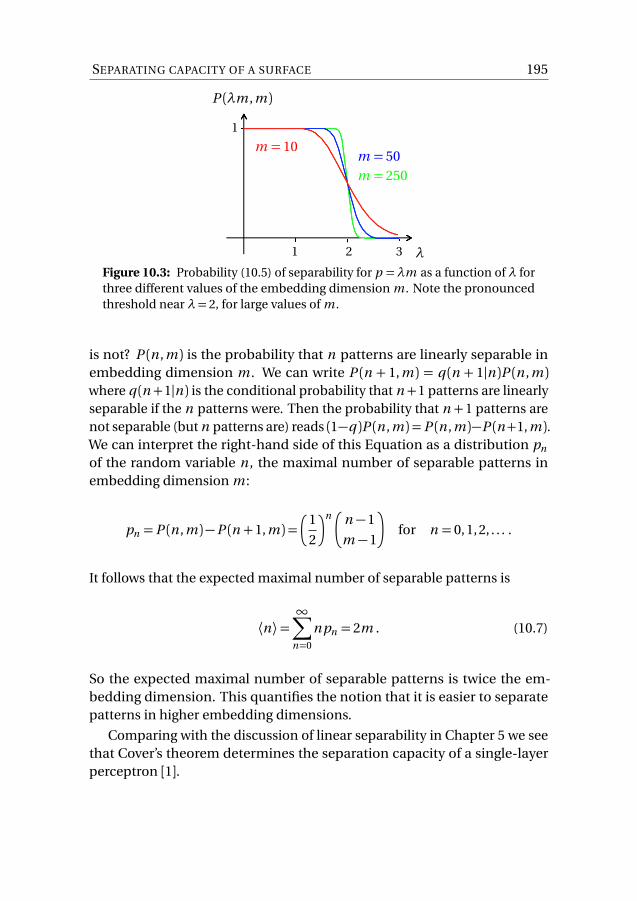
SEPARATING CAPACITY OF A SURFACE 195
λ
P (λm , m )
m = 250m = 50
m = 10
1 2 3
1
Figure 10.3: Probability (10.5) of separability for p =λm as a function of λ forthree different values of the embedding dimension m . Note the pronouncedthreshold near λ= 2, for large values of m .
is not? P (n , m ) is the probability that n patterns are linearly separable inembedding dimension m . We can write P (n + 1, m ) = q (n + 1|n )P (n , m )where q (n +1|n ) is the conditional probability that n +1 patterns are linearlyseparable if the n patterns were. Then the probability that n +1 patterns arenot separable (but n patterns are) reads (1−q )P (n , m ) = P (n , m )−P (n+1, m ).We can interpret the right-hand side of this Equation as a distribution pn
of the random variable n , the maximal number of separable patterns inembedding dimension m :
pn = P (n , m )−P (n +1, m ) =�
1
2
�n�
n −1
m −1
�
for n = 0, 1, 2, . . . .
It follows that the expected maximal number of separable patterns is
⟨n⟩=∞∑
n=0
npn = 2m . (10.7)
So the expected maximal number of separable patterns is twice the em-bedding dimension. This quantifies the notion that it is easier to separatepatterns in higher embedding dimensions.
Comparing with the discussion of linear separability in Chapter 5 we seethat Cover’s theorem determines the separation capacity of a single-layerperceptron [1].

196 RADIAL BASIS-FUNCTION NETWORKS
x1
x2
u1
u2
u3
u4
W1
W2
W3
W4
linear output
O =∑m
j=1 Wj u j
Figure 10.4: Radial basis-function network for N = 2 inputs and m = 4 radialbasis functions (10.8). The output neuron has weights W and zero threshold.
10.2 Radial basis-function networks
The idea behind radial basis-function networks is to parameterise the func-tions u j (x ) in terms of weight vectors w j , and to use an unsupervised-learning algorithm (Chapter 9) to find weights that separate the input data.A common choice [2] are radial basis functions of the form:
u j (x ) = exp�
−1
2s 2j
�
�x −w j
�
�
2 �
. (10.8)
These functions are not of the finite-order polynomial form that was assumedin Cover’s theorem. This means that the theorem does not strictly apply. Theparameters s j parameterise the widths of the radial basis functions. In thesimplest version of the algorithm they are set to unity. Other choices forradial basis functions are given by Haykin [2].
Figure 10.2 shows a radial basis-function network for N = 2 and m = 4.The four neurons in the hidden layer stand for the four radial basis functions(10.8) that map the inputs to four-dimensional u -space. The network lookslike a perceptron (Chapter 5). But here the hidden layers work in a differentway. Perceptrons have hidden McCulloch-Pitts neurons that compute non-local outputs σ(w j · x − θ ). The output of radial basis functions u j (x ), bycontrast, is localised in input space [Figure 10.5(left)]. We saw in Section 7.1how to make localised basis functions out of McCulloch-Pitts neurons withsigmoid activation functions σ(b ), but one needs two hidden layers to dothat [Figure 10.5(right)].
Radial basis functions produce localised outputs with a single hiddenlayer, and this makes it possible to divide up input space into localised re-

RADIAL BASIS-FUNCTION NETWORKS 197
x1
x2
x1
x2
Figure 10.5: Comparison between radial-basis function network and percep-tron. Left: the output of a radial basis function is localised in input space. Right:to achieve a localised output with sigmoid units one needs two hidden layers(Section 7.1). One layer determines the lightly shaded cross, the second layerlocalises the output to the darker square.
gions, each corresponding to one radial basis function. Imagine for a mo-ment that we have as many radial basis functions as input patterns. In thiscase we can simply take w µ = x (µ) for µ = 1, . . . , p . Then the classificationproblem can be written as
UW = t , (10.9)
where U is the symmetric p ×p matrix with entries Ui j = u j (x i ). Here weused that the output unit is linear. If all patterns are pairwise different,x (µ) 6= x (ν) for µ 6= ν, then the matrix U is invertible [2], and the solution ofthe classification problem reads W =U−1t .
In practice one can get away with fewer radial basis functions by choosingtheir weights to point in the directions of clusters of input data. To this endone can use unsupervised competitive learning (Algorithm 12), where thewinning unit is defined to be the one with largest u j . How are the widths s j
determined? The width s j of radial basis function u j (x ) is taken to be equalto the minimum distance between w j and the centers of the surroundingradial basis functions. Once weights and widths of the radial basis functionsare found, the weights of the output neuron are determined by minimising
H =1
2
∑
µ
�
t (µ)−O (µ)�2
(10.10)
with respect to W . If the problem is linearly separable in the u -plane, thenthe minimum is given by Equation (5.23). An approximate solution can beobtained by stochastic gradient descent on H keeping the parameters of the

198 RADIAL BASIS-FUNCTION NETWORKS
Algorithm 12 radial basis functions
1: initialise the weights w j k independently randomly from [−1, 1];2: set all widths to s j = 0;3: for t = 1, . . . , T do4: feed randomly chosen pattern x (µ);5: determine winning unit j0: u j0
≥ u j for all values of j ;6: update widths: s j =min j 6=k |w j −w k |;7: update only winning unit: δw j0
=η(x (µ)−w j0);
8: end for9: end;
radial basis functions fixed. Cover’s theorem indicates that the problem ismore likely to be separable if the embedding dimension m is higher. Figure10.6 shows an example for a non-linear decision boundary found by thisalgorithm.
10.3 Summary
Radial basis-function networks are similar to the perceptrons described inChapters 5 to 7, in that they are feed-forward networks designed to solveclassification problems. The outputs work in similar ways.
A fundamental difference is that the parameters of the radial basis func-tions are determined by unsupervised learning, whereas perceptrons are
decisionboundary
t =+1
t =−1
x2
x1
m classification error
5 0.26
20 0.06
Figure 10.6: Left: non-linear decision boundary found by a radial basis-function network for m = 20 (schematic). Right: classification error for differentembedding dimensions. The decision boundary is not yet quite perfect form = 20, it still cuts the corners a little bit.

FURTHER READING 199
trained using supervised learning for all units.
While McCulloch-Pitts neurons compute weights to minimise their out-put from given targets, the radial basis functions compute weights by max-imising u j as a function of j . The algorithm for finding the weights of theradial basis functions is summarised in Algorithm 12.
Further, as opposed to the deep networks from Chapter 7, radial basis-function networks have only one hidden layer, and a linear output neuron.Radial-basis function nets learn using a hybrid scheme: unsupervised learn-ing for the parameters of the radial basis functions, and supervised learningfor the weights of the output neuron.
10.4 Further reading
For a proof of Cover’s theorem see Ref. [96]. Radial-basis function networksare discussed by Haykin in Chapter 5 of his book [2]. Hertz, Krogh and Palmer[1] have a brief Section on radial basis-function nets too (their Section 9.7).They use normalised radial basis functions
u j (x ) =exp
�
− 12s 2
j
�
�x −w j
�
�
2 �
∑mk=1 exp
�
− 12s 2
j
�
�x −w j
�
�
2 � , (10.11)
instead of Equation (10.8).
It has been argued that radial-basis function nets do not generalise aswell as perceptrons do [97]. To solve this problem, Poggio and Girosi [98]suggested to determine the parameters w j of the radial basis function bysupervised learning, using stochastic gradient descent.
10.5 Exercises
Expected maximal number of separable patterns. Show that the sum inEquation (10.7) sums to 2m .

200 RADIAL BASIS-FUNCTION NETWORKS
10.6 Exam questions
10.6.1 Radial basis functions for XOR
(a) Show that the Boolean XOR problem (Table 10.1) cannot be solved by asimple perceptron.(b) The problem can be solved by transforming input space using radial-basisfunctions, and applying a simple perceptron with linear activation functionto the transformed input data. Show that the two-dimensional BooleanXOR problem can be solved using the two radial basis functions g1(x (µ)) =exp(−|x (µ) −w 1|2) and g2(x (µ)) = exp(−|x (µ) −w 2|2) with w 1 = (1,1)T andw 2 = (0, 0)T. Draw the positions of the four input patterns in the transformedspace with coordinates g1 and g2, encoding the different target values. Hint:to compute the states of input patterns in the transformed space (g1, g2)T,use the following approximations: exp(−1) ≈ 0.37, exp(−2) ≈ 0.14. Explainthe term decision boundary, draw a decision boundary for the XOR problem,and give the corresponding weights and thresholds for the simple perceptron.(1p).
x1 x2 t0 0 00 1 11 0 11 1 0
Table 10.1: Inputs and target values for the XOR problem. Question 10.6.1.
10.6.2 Radial basis functions
(a) Illustrate the problem given in Table 10.2 graphically. Explain whether ornot it can be solved by a simple perceptron with three input units, and one
output unit O (µ) = sgn(∑3
j=1 Wj x(µ)j −Θ), where Wj is the weight from unit j
to the output with threshold Θ. (0.5 p).(b) Show that this problem can be solved following the three steps below.
1. Transform the inputs (x1, x2, x3) to two-dimensional coordinates (g1, g2)

EXAM QUESTIONS 201
using radial basis functions:
g1(x(µ)) = exp(−|x (µ)−w 1|2), with w 1 = (0, 0, 0)T ,
g2(x(µ)) = exp(−|x (µ)−w 2|2), with w 2 = (1, 0, 1)T .
Here x (µ) = (x (µ)1 , x(µ)2 , x
(µ)3 )
T, and | · · · | denotes the norm of a vector.Plot the positions of the eight input patterns listed in Table 10.2 in(g1, g2)-coordinates, encoding the different target outputs. Hint: tocompute g i (x (µ)) use the following approximations: exp(−1) ≈ 0.37,exp(−2)≈ 0.14, exp(−3)≈ 0.05. (0.5 p).
2. Use the transformed input data as inputs to a simple perceptron withsgn(· · · ) activation function. In the plot you drew in the previous step,draw also a decision boundary that solves the problem when a simpleperception is applied to the transformed data. (0.5 p).
3. Compute a weight vector and a threshold for the simple perceptroncorresponding to the decision boundary you drew in the previous step.(0.5p)
µ x(µ)1 x
(µ)2 x
(µ)3 t (µ)
1 0 1 0 −12 1 0 1 +13 0 0 0 +14 1 0 0 −15 1 1 0 −16 0 0 1 −17 0 1 1 −18 1 1 1 −1
Table 10.2: Inputs and target values. Question 10.6.2.

202 REINFORCEMENT LEARNING
11 Reinforcement learning
Reinforcement learning is a modified version of supervised learning. In thelatter case, target patterns t (µ) are available for all input patterns x (µ). Inpractice, less information may be needed. For instance, the feedback mayconsist only of a single bit of information (output O1, . . . , OM right or wrong).
To show how neural networks can learn from incomplete feedback, Iexplain the associative reward penalty algorithm in the following. This algo-rithm is formulated in terms of stochastic output units. So we must brieflydiscuss these first.
11.1 Stochastic output units
Consider a set of output units Si with targets t(µ)i =±1. As energy function
we take Equation (6.4):
H =1
2
∑
iµ
�
t(µ)i −O
(µ)i
�2. (11.1)
In Chapters 5 to 8 the output neurons were deterministic functions of theirinputs, either sigmoid, tanh, or softmax functions. Reinforcement learning,by contrast, works with stochastic output units. The idea is the same asin Chapters 3 and 4: stochastic output units can explore a wider range ofpossible states which may in the end lead to a better solution. Usually onlythe output units are stochastic. The weights of hidden neurons are trainedas usual by backpropagation.
For the output neurons we use the stochastic update rule (3.2):
O(µ)i =
¨
+1, with probabilityP (b (µ)i ) ,
−1, with probability 1−P (b (µ)i ) ,(11.2a)
where bi is the local field with activation function equal to the identity func-tion:
b(µ)i =
∑
j
Wi j V(µ)
j , (11.2b)
andP (b ) = (1+e −2βb )−1. The parameter β−1 is the noise level, as in Chapter3. The Vj represent hidden neurons or inputs.

STOCHASTIC OUTPUT UNITS 203
How does one train the weights Wi j of the stochastic neurons? To for-mulate a definite learning rule, we average over the stochastic dynamics ofthe network, just as in Chapter 3. But how can one learn on average? Onepossibility is to compare the average output with the desired output. This
corresponds to replacing O(µ)i by ⟨O (µ)i ⟩ in the energy function:
H =∑
iµ
�
t(µ)i −⟨O
(µ)i ⟩
�2with ⟨O (µ)i ⟩= tanh
�
βb(µ)i
�
. (11.3)
Here we used Equation (3.11). Gradient descent gives for the weight changesin the output layer:
δWmn =η∂H
∂ wmn=η
∑
iµ
(t (µ)i −⟨O(µ)i ⟩)β (1−⟨O
(µ)i ⟩
2)δi m V (µ)n . (11.4)
This update rule contains a sum over patterns (batch training). The corre-sponding sequential rule can be written in the usual form:
δWmn =ηδ(µ)m V (µ)n with δ(µ)m = (t
(µ)m −⟨O
(µ)m ⟩)β (1−⟨O
(µ)i ⟩
2) . (11.5)
The factor β (1−⟨O (µ)m ⟩2) corresponds to the factor g ′(B (µ)m ) in Equation (6.7).One can show that this rule decreases the energy, on average. To this end we
use that O(µ)i =±1 and t
(µ)i =±1. This means that the energy function can be
rewritten asH =
∑
iµ
�
1− t(µ)i O
(µ)i
�
. (11.6)
The change in the average energy due to the weight increment (11.5) is
δ⟨H ⟩=∑
mn
∂ ⟨H ⟩∂Wmn
δWmn =−∑
mniµ
t(µ)i
∂ ⟨O (µ)i ⟩∂Wmn
δWmn . (11.7)
Using
∂ ⟨O (µ)i ⟩∂Wmn
=β [1− tanh2(βb(µ)i )]δi m V (µ)n (11.8)
one finds
δ⟨H ⟩=−ηβ2∑
mnµ
[1− tanh2(βb (µ)m )]2[1− t (µ)m tanh(βb (µ))m ](V (µ)n )2 < 0 . (11.9)

204 REINFORCEMENT LEARNING
Returning to the learning rule (11.5), note that the formula for the error is
sometimes written without the factor β (1−⟨O (µ)m ⟩2) (in Ref. [1] for instance):
δWmn =ηδ(µ)m V (µ)n with δ(µ)m = t (µ)m −⟨O
(µ))m ⟩ . (11.10)
This choice corresponds to using the energy function (7.32), see Section 7.2.3.
11.2 Associative reward-penalty algorithm
Now consider a learning problem where the network receives incompleteinformation about the target patterns. In the simplest case it might justreceive a reinforcement signal,
r =
¨
+1, reward,
−1, penalty.(11.11)
The network gets positive feedback (r = 1) when its output match the targetswell (but perhaps not perfectly), and it receives negative feedback (r =−1) ifthe match is not good. The idea of reinforcement learning is to use outputsthat receive positive feedback instead of the target values that are not known:
t(µ)i =
¨
O(µ)i , if r (µ) =+1
−O(µ)i , if r (µ) =−1.
(11.12)
Substituting Equation (11.12) into the stochastic learning rule (11.10) yieldsthe learning rule for the associative reward-penalty algorithm:
δWi j =
¨
η(+)(O (µ)i −⟨O (µ)i ⟩)V(µ)
j reward (r (µ) =+1)
η(−)(−O(µ)i −⟨O (µ)i ⟩)V
(µ)j penalty (r (µ) =−1),
(11.13)
Often η(+) is taken to be larger than η(−), for example η(+)/η(−) ≈ 10 or 100 [1].A special case is a network with only one binary output neuron. In this
case reinforcement learning determines correct output pattern (−O (µ) iscorrect if O (µ) is wrong), so the target patterns t (µ) are precisely reconstructedin this way. But there is no general convergence proof for the algorithm formore than one binary output unit.

SUMMARY 205
11.3 Summary
In Chapters 5 to 8 we discussed how to train networks to correctly associateinput/output pairs (x (µ), t (µ)) in a training set (supervised learning). Chapters9 and 10 described unsupervised learning where the network learns with-out any feedback. The reinforcement algorithm introduced in the presentChapter is in between. It learns from incomplete feedback. Not all targetsare known to the network. The feedback may simply be r =±1 (good or badsolution). The associative reward-penalty algorithm uses this feedback tobuild up a training set that allows the network to learn.
11.4 Further reading
Reinforcement learning has developed substantially in recent years [99–101].Many recent studies on reinforcement learning use the Q-learning algorithm[100, 101]. A recent application of reinforcement learning is AlphaGo, analgorithm that learnt to play the game of Go. How it works is described inthis blog.

206 REINFORCEMENT LEARNING

207
PART IV
APPENDIX
12 Solutions
Chapter 2
2.7.1 One-step error probability
2.7.2 Hopfield network
2.7.3 Hopfield network
2.7.4 Energy function for deterministic Hopfield network
2.7.5 Diluted Hopfield network
2.7.6 Mixed states
Chapter 3
3.9.1 Stochastic Hopfield network
Chapter 5
5.8.1 Linear separability of Boolean functions
5.8.2 Boolean functions
5.8.3 Linearly inseparable problem
5.8.4 Perceptron with one hidden layer

208 SOLUTIONS
Chapter 6
6.7.1 Multilayer perceptron
6.7.2 Backpropagation
6.7.3 Backpropagation
6.7.4 Backpropagation
6.7.5 Backpropagation
6.7.6 True/false questions
Chapter 7
7.10.1 Parity function
7.10.2 Softmax outputs
Chapter 9
9.6.1 Oja’s rule
9.6.2 Oja’s rule
9.6.3 Covariance matrices
9.6.4 Kohonen net
Chapter 10
10.6.1 Radial basis functions for XOR
10.6.2 Radial basis functions

209
Figure 13.1: Reproduced from xkcd.com/1838 under the creative commonsattribution-noncommercial 2.5 license.
13 Some linear algebra

210 SOME LINEAR ALGEBRA

BIBLIOGRAPHY 211
Bibliography
[1] HERTZ, J, KROGH, A & PALMER, R 1991 Introduction to the Theory ofNeural Computation. Addison-Wesley.
[2] HAYKIN, S 1999 Neural Networks: a comprehensive foundation. NewJersey: Prentice Hall.
[3] HORNER, H, Neuronale Netze, [Online; accessed 8-November-2018].
[4] GOODFELLOW, I, Y., B & COURVILLE, A, Deep Learning, [Online; accessed5-September-2018].
[5] NIELSEN, M, Neural Networks and Deep Learning, [Online; accessed13-August-2018].
[6] LECUN, A, BENGIO, Y & HINTON, G 2015 Deep learning. Nature 521,463.
[7] MACHEREY, W, KRIKUN, M, CAO, Y, GAO, Q, MACHEREY, K, KLINGNER,J, SHAH, A, JOHNSON, M, LIU, X, KAISER, L, GOUWS, S, KATO, Y, KUDO,T, KAZAWA, H, STEVENS, K, KURIAN, G, PATIL, N, WANG, W, YOUNG, C,SMITH, J, RIESA, J, RUDNICK, A, VINYALS, O, CORRADO, G, HUGHES, M& DEAN, J 2016 Google’s neural machine translation system: bridgingthe gap between Human and machine translation arxiv:1609.08144.
[8] DEEPMIND, AlphaGo, [Online; accessed: 20-August-2018].
[9] BRAIN MAPS, An interactive multiresolution brain atlas; SMI32-immunoreactive pyramidal neuron in medial prefrontal cortex ofmacaque, brainmaps.org, [Online; accessed 14-August-2018].
[10] GABBIANI, F & METZNER, W 1999 Encoding and processing of sensoryinformation in neuronal spike trains. Journal of Experimental Biology202 (10), 1267.
[11] MCCULLOCH, W & PITTS, W 1943 A logical calculus of the ideas imma-nent in nervous activity. Bull. Math. Biophys. 5, 115.
[12] ROSENBLATT, F 1958 A probabilistic model for information storage andorganization in the brain. Psychological Review 65, 386.

212 BIBLIOGRAPHY
[13] ROSENBLATT, F 1958 The perceptron: A probabilistic model for infor-mation storage and organization in the brain. Psychological Rev. 65,386.
[14] HOPFIELD, J. J, Hopfield network, [Online; accessed 14-August-2018].
[15] MÜLLER, B, REINHARDT, J & STICKLAND, M. T 1999 Neural Networks: acomprehensive foundation. Heidelberg: Springer.
[16] AMIT, D. J, GUTFREUND, H & SOMPOLINSKY, H 1985 Spin-glass modelsof neural networks. Phys. Rev. A 32, 1007.
[17] AMIT, D. J & GUTFREUND, H 1987 Statistical mechanics of neural net-works near saturation. Ann. Phys. 173, 30.
[18] ZIRNBAUER, M 1994 Another critique of the replica trick arxiv:cond-mat/9903338.
[19] STEFFAN, H & KUEHN, R 1994 Replica symmetry breaking in attractorneural network models arxiv:cond-mat/9404036.
[20] VOLK, D 1998 On the phase transition of Hopfield networks – anotherMonte Carlo study. Int. J. Mod. Phys. C 9, 693.
[21] POTVIN, J. Y & SMITH, K. A 1999 Artificial neural networks for com-binatorial optimization. In Handbook of Metaheuristics (ed. G F. &G Kochenberger). Heidelberg: Springer.
[22] MANDZIUK, J 2002 Neural networks for the n-Queens problem: a review.Control and Cybernetics 31, 217, Special issue on neural networks foroptimization and control.
[23] WATERMAN, M 1995 Introduction to Bioinformatics. Prentice Hall.
[24] HOPFIELD, J. J & TANK, D. W 1985 Neural computation of decisions inoptimisation problems. Biol. Cybern. 52, 141.
[25] PRESS, W, TEUKOLSKY, S, VETTERLING, W & FLANNERY, W 1992 Numeri-cal Recipes in C: The Art of Scientific Computing, second edition. NewYork: Cambridge University Press.

BIBLIOGRAPHY 213
[26] KAMPEN, N. V 2007 Stochastic processes in physics and chemistry. NorthHolland.
[27] MEHLIG, B, HEERMANN, D. W & FORREST, B. M 1992 Hybrid MonteCarlo method for condensed-matter systems. Phys. Rev. B 45, 679–685.
[28] BINDER, K, ed. 1986 Monte Carlo Methods in Statistical Physics. Heidel-berg: Springer.
[29] NEWMAN, M. E. J & BARKEMA, G. T 1999 Monte Carlo Methods in Statis-tical Physics. Oxford: Clarendon Press.
[30] SALAMON, P, SIBANI, P & FROST, R 2002 Facts, conjectures, and improve-ments for simulated annealing. SIAM.
[31] MACHINE LEARNING REPOSITORY UNIVERSITY OF CALIFORNIA IRVINE,archive.ics.uci.edu/ml, [Online; accessed 18-August-2018].
[32] FISHER, R. A 1936 The use of multiple measurements in taxonomicproblems. Ann. Eugenics 7, 179.
[33] LÖWE, M 1998 In the storage capcaity of Hopfield models with corre-lated patterns. Ann. Prob. 8, 1216.
[34] MINSKY, M & PAPERT, S 1969 Perceptrons. An Introduction to Computa-tional Geometry. MIT Press.
[35] KANAL, L. N 2001 Perceptrons. In International Encyclopedia of theSocial and Behavioral Sciences.
[36] LECUN, Y, BOTTOU, L, ORR, G. B & MÜLLER, K.-R 1998 Efficient backprop. In Neural networks: tricks of the trade (ed. G. B Orr & K.-R Müller).Springer.
[37] NESTEROV, Y 1983 A method of solving a convex programming problemwith convergence rate o(1/k 2). Soviet Mathematics Doklady 27, 372.
[38] SUTSKEVER, I 2013 Training recurrent neural networks. PhD thesis,University of Toronto, [Online; accessed 27-October-2018].

214 BIBLIOGRAPHY
[39] HANSON, S. J & PRATT, L. Y 1989 Comparing biases for minimal networkconstruction with backpropagation. In Advances in Neural InformationProcessing Systems 1.
[40] KROGH, A & HERTZ, J. A 1992 A simple weight decay can improve gen-eralization. In Advances in Neural Information Processing Systems 4.
[41] HASSIBI, B & G.STORK, D 1993 Second order derivatives for networkpruning: Optimal brain surgeon. In Advances in Neural InformationProcessing Systems 5.
[42] LECUN, Y, DENKTER, J. S & SOLLA, S 1990 Optimal brain damage. In Ad-vances in Neural Information Processing Systems 2 (ed. D. S Touretzky),p. 598.
[43] RUMELHART, D. E, HINTON, G. E & WILLIAMS, R. J 1986 Learning internalrepresentations by error propagation. In Parallel distributed processing:explorations in the microstructure of cognition (ed. D. E Rumelhart &J. L MCClelland).
[44] HORNIK, K, STINCHOME, M & WHITE, H 1989 Neural networks areuniversal approximators. Neural Networks 2, 359.
[45] CVITANOVIC, P, ARTUSO, G, MAINIERI, R, TANNER, G & VATTAY, G, chaos-book.org/version15 (Niels Bohr Institute, Copenhagen 2015), Lya-punov exponents, [Online; accessed 30-September-2018].
[46] PENNINGTON, J, SCHOENHOLZ, S. S & GANGULI, S 2017 Resurrectingthe sigmoid in deep learning through dynamical isometry: theory andpractice. In Advances in Neural Information Processing Systems 30.
[47] GLOROT, X, BORDES, A & BENGIO, Y 2011 Deep sparse rectifier neuralnetworks. In Proceedings of Machine Learning Research.
[48] SUTSKEVER, I, MARTENS, J, DAHL, G & HINTON, G 2013 On the impor-tance of initialization and momentum in deep learning ACM DigitalLibrary.
[49] GLOROT, X & BENGIO, Y 2010 Understanding the difficulty of trainingdeep feedforward neural networks. In Proceedings of Machine LearningResearch.

BIBLIOGRAPHY 215
[50] SRIVASTAV, N, HINTON, G, KRISHEVSKY, A, SUTSKEVER, I & SALKHUTDI-NOV, R 2014 Dropout: A simple way to prevent neural networks fromoverfitting Journal of Machine Learning Research.
[51] FRANKLE, J & CARBIN, M 2018 The lottery ticket hypothesis: Findingsmall, trainable neural networks arxiv:1803.03635.
[52] IMAGENET, image-net.org, [Online; accessed 3-September-2018].
[53] IOFFE, S & SZEGEDY, C 2015 Batch normalization: Accelerating deepnetwork training by reducing internal covariate shift arxiv:1502.03167.
[54] SANTURKAR, S, TSIPRAS, D, ILYAS, A & MADRY, A 2018 How does batchnormalization help optimization? (No, it is not about internal covariateshift) arxiv:1805.11604.
[55] KRIZHEVSKY, A, SUTSKEVER, I & HINTON, G. E 2012 Imagenet classifica-tion with deep convolutional neural networks. In Advances in NeuralInformation Processing Systems 25.
[56] TENSORFLOW, tensorflow.org, [Online; accessed 3-September-2018].
[57] LECUN, Y & CORTES, C, MNIST, [Online; accessed 3-September-2018].
[58] KERAS, Keras, [Online; accessed 26-September-2018].
[59] THEANO, Theano, [Online; accessed 26-September-2018].
[60] PYTORCH, PyTorch, [Online; accessed 28-October-2018].
[61] SMITH, L. N 2015 Cyclical learning rates for training neural networksarxiv:1506.01186.
[62] CIRESAN, D, MEIER, U & SCHMIDHUBER, J 2012 Multi-column deepneural networks for image classification arxiv:1202.2745.
[63] KOZIELSKI, M, FORSTER, J & NEY, H 2012 Moment-based image nor-malization for handwritten text recognition. In Proceedings of the 2012International Conference on Frontiers in Handwriting Recognition.
[64] PASCAL VOC DATA SET, Pascal VOC, [Online; accessed 6-September-2018].

216 BIBLIOGRAPHY
[65] REDMON, J, DIVVALA, S, GIRSHICK, R & FARHADI, A, You only look once:Unified, real-time object detection, arxiv:1506.02640.
[66] RUSSAKOVSKY, O, DENG, J, SU, H, KRAUSE, J, SATHEESH, S, MA, S, HUANG,Z, KARPATHY, A, KHOSLA, A, BERNSTEIN, M, BERG, A. C & FEI-FEI, L 2014Imagenet large scale visual recognition challenge arxiv:1409.0575.
[67] HE, K, ZHANG, X, REN, S & SUN, J 2015 Deep residual learning for imagerecognition arxiv:1512.03385.
[68] LI, F, JOHNSON, J & YEUNG, S, CNN architectures, CNN architectures,[Online; accessed 23-September-2018].
[69] HU, J, SHEN, L & SUN, G 2018 Squeeze-and-excitation networksarxiv:1709.01507.
[70] Tensor processing unit, github.com/tensorflow/tpu, [Online; accessed23-September-2018].
[71] SZEGEDY, C, LIU, W, JIA, Y, SERMANET, P, REED, S, ANGUELOV, D, ERHAN,D, VANHOUCKE, V & RABINOVICH, A 2014 Going deeper with convolu-tions arxiv:1409.4842.
[72] ZENG, X, OUYANG, W, YAN, J, LI, H, XIAO, T, WANG, K, LIU, Y, ZHOU,Y, YANG, B, WANG, Z, ZHOU, H & WANG, X 2016 Crafting GBD-net forobject detection arxiv:1610.02579.
[73] HERN, A, Computers now better than humans at recognising and sort-ing images, The Guardian, [Online; accessed 26-September-2018].
[74] KARPATHY, A, What I learned from competing against a convnet onimagenet, blog, [Online; accessed 26-September-2018].
[75] KHURSHUDOV, A, Suddenly, a leopard print sofa appears, [Online; ac-cessed 23-August-2018].
[76] KARPATHY, A, ILRSVC labeling interface, [Online; accessed 26-September-2018].
[77] GEIRHOS, R, TEMME, C. R. M, RAUBER, J, SCHÜTT, H. H, BETHGE, M& WICHMANN, F. A 2018 Generalisation in Humans and deep neuralnetworks arxiv:1808.08750.

BIBLIOGRAPHY 217
[78] SZEGEDY, C, ZAREMBA, W, SUTSKEVER, I, BRUNA, J, ERBAN, D. A ND GOOD-FELLOW, I & FERGUS, R 2013 Intriguing properties of neural networksarxiv:1312.6199.
[79] NGUYEN, A, YOSINSKI, J & CLUNE, J 2015 Deep neural networks areeasily fooled: high confidence predictions for unrecognisable imagesarxiv:1412.1897.
[80] YOSINSKI, J, CLUNE, J, NGUYEN, A, FUCHS, T & LIPSON, H 2015 Under-standing neural networks through deep visualization arxiv:1506.06579.
[81] CHOROMANSKA, A, HENAFF, M, MATHIEU, M, BEN AROUS, G & LECUN,Y 2014 The loss surfaces of multilayer networks arxiv:1412.0233.
[82] KIRKPATRICK, J, PASCANU, R, RABINOWITZ, N, VENESS, J, DESJARDINS, G,RUSU, A. A, MILAN, K, QUAN, J, RAMALHO, T, GRABSKA-BARWINSKA, A,HASSABIS, D, CLOPATH, C, KUMARAN, D & HADSELL, R 2016 Overcomingcatastrophic forgetting in neural networks arxiv:1612.00796.
[83] SETTLES, B 2009 Active Learning Literature Survey. Tech. Rep. 1648.University of Wisconsin–Madison.
[84] SUTSKEVER, I, VINYALS, O & LE, Q. V 2014 Sequence to sequence learn-ing with neural networks arxiv:1409.3215.
[85] LIPTON, Z. C, BERKOWITZ, J & ELKAN, C 2015 A critical review of recur-rent neural networks for sequence learning arxiv:1506.00019.
[86] PASCANU, R, MIKOLOV, T & BENGIO, Y 2012 On the difficulty of trainingrecurrent neural networks arxiv:1211.5063.
[87] HOCHREITER, S & SCHMIDHUBER, J 1997 Long short-term memory.Neural Computation 9, 1735.
[88] PAPINENI, K, ROUKOS, S, WARD, T & ZHU, W.-J 2002 Bleu: a methodfor automatic evaluation of machine translation. In Proceedings of the40th annual meeting on association for computational linguistics, p.311.
[89] DOYA, K 1993 Bifurcations of recurrent neural networks in gradientdescent learning. IEEE Transactions on Neural Networks 1, 75.

218 BIBLIOGRAPHY
[90] KARPATHY, A, The unreasonable effectiveness of recurrent neural net-works, webpage, [Online; accessed 4-October-2018].
[91] WILKINSON, M, BEZUGLYY, V & MEHLIG, B 2009 Fingerprints of randomflows? Phys. Fluids 21, 043304.
[92] OJA, E 1982 A simplified neuron model as a principal component ana-lyzer. J. Math. Biol. 15, 267.
[93] PRITCHARD, J. K, STEPHENS, M & DONNELLY, P 2000 Inference of popu-lation structure using multilocus genotype data. Genetics 155, 945.
[94] Human genome diversity project, HGDP, [Online; accessed 10-October-2018].
[95] COVER, T. M 1965 Geometrical and statistical properties of systemsof linear inequalities with applications in pattern recognition. IEEETrans. on electronic computers p. 326.
[96] SOMPOLINSKY, H, Introduction: the perceptron, The perceptron, [On-line; accessed 9-October-2018].
[97] WETTSCHERECK, D & DIETTERICH, T 1992 Improving the performanceof radial basis function networks by learning center locations. In Ad-vances in Neural Information Processing Systems 4, pp. 1133–1140. Mor-gan Kaufmann.
[98] POGGIO, T & GIROSI, F 1990 Networks for approximation and learning.In Proceedings of the IEEE, , vol. 78, p. 1481.
[99] SUTTON, R. S, ed. 1992 A special issue of machine learning on rein-forcement learning, reprinted from Machine Learning Vol. 8, Nos. 3–4.Springer.
[100] WIERING, M & VAN OTTERLO, M 1999 Reinforcement learning. Heidel-berg: Springer.
[101] SZEPESVARI, C 2010 Algorithms for reinforcement learning. In Synthe-sis Lectures on Artificial Intelligence and Machine Learning (ed. R. JBrachmann & T Dietterich). Morgan and Claypool Publishers.

INDEX 219
Index
accelerated gradient, 95activation function, 6, 7active, 4, 113active learning, 143adversarial images, 142approximation, 100array of inputs, 123associative reward penalty, 182associative-memory problem, 10asynchronous updating, 5attractor, 12, 17auto association, 61axon, 3
backpropagation, 81backpropagation through time, 151basis function, 101batch normalisation, 111batch training, 72, 82, 183Bernoulli trial, 21bias, 64bidirectional recurrent net, 157bilingual evaluation understudy, 158binary, 10Boltzmann distribution, 46, 56Boltzmann machine, 9bond, 24Boolean function, 67bottleneck, 112
cell body, 3central limit theorem, 20central-limit theorem, 2, 117cerebal cortex, 3chain rule, 79, 109channel, 124classification, 61classification accuracy, 92, 129classification error, 90, 116, 127cluster, 159, 165competitive learning, 165competitive learning rule, 165configuration space, 12continuum approximation, 169continuum limit, 169convergence phase, 168, 172convolution, 124convolution layers, 124convolutional network, 123cost function, 114covariance, 19covariance matrix, 164covariate shift, 88, 121Cover’s theorem, 175cross entropy, 116cross validation, 90cross-entropy error, 92cross-talk term, 19

220 INDEX
data set augmentation, 120, 137, 141decision boundary, 66deep belief network, 9deep learning, 1, 62, 64deep networks, 84, 106delta rule, 81dendrite, 3dendrites, 3detailed balance, 57deterministic, 30digest, 52diminishing returns, 131double digest problem, 52drop out, 118, 137duality, 149dynamical networks, 146dynamical systems theory, 158
early stopping, 90elastic net, 168embedding, 174embedding dimension, 175energy function, 23epoch, 82error, 80, 148, 153error avalanche, 44error function, 22excitatory, 6expanding training set, 118, 120
familiarity, 2, 159, 160feature map, 105feature maps, 123feed forward layout, 80, 82feed forward network, 145feedback, 145fingerprint, 52
firing rate, 111free energy, 36
generalisation, 76generalise, 93gradient descent, 71
Hamiltonian, 23Hamming distance, 11Heaviside, 6, 73Hebb’s rule, 2, 9, 14, 160Hessian, 96hidden layer, 61homogeneously linearly separable, 175
idempotent, 16image classification, 135inactive, 4inertia, 94inhibitory, 6input plane, 65input scaling, 86integer linear programming, 51inverted pattern, 18, 26, 36iris data set, 61iteration, 82
k means clustering, 3k queens problem, 51kink, 168, 172Kohonen’s rule, 167Kronecker delta, 19, 71, 80
L1 regularisation, 93L2 pooling, 126L2 regularisation, 93Lagrange multiplier, 53, 97Lagrangian, 97

INDEX 221
leaky integrate-and-fire, 111learning rate, 69, 71linear unit, 70linearly dependent, 71linearly separable, 67, 174local field, 13local neurons, 75local receptive field, 124local rule, 81log likelihood, 114log normal, 109long short term memory, 156Lyapunov exponent, 110Lyapunov vectors, 110
machine translation, 1magnet, 9Markov chain, 56Markov chain Monte Carlo, 3, 9, 56max norm regularisation, 119max pooling, 126McCulloch-Pitts neuron, 2mean field, 34mean field theory, 34membrane potential, 111memoryless, 56Metropolis algorithm, 56, 57mini batch, 82, 88mixed state, 26momentum, 94momentum constant, 94
neighbourhood function, 168nested, 78neural dynamics, 5neural networks, 1neuron, 3
non linear units, 72non local, 178
object recognition, 1Oja’s rule, 162, 164order disorder transition, 30order parameter, 32ordering phase, 168, 172orthogonal patterns, 23, 29, 63outer product, 15overfitting, 90, 93, 117–120, 123, 126,
130, 137, 141overlap matrix, 63
parity function, 104partition function, 46, 56pattern, 10perceptron, 4, 61phase diagram, 47phase transition, 45pooling layer, 124principal component, 3, 88principal direction, 88pruning, 96
radial basis functions, 175, 178random pattern, 10, 19rectified linear unit, 112recurrent backpropagation, 146recurrent network, 1recurrent networks, 145redundancy, 159region of attraction, 13regularisation, 93, 117reinforcement learning, 2, 172reinforcement signal, 184ReLU, 112, 137replica, 46

222 INDEX
residual network, 111, 138, 140, 156restriction map, 52restriction site, 52retrieval, 9right Cauchy Green matrix, 110
Sanger’s rule, 164scalar product, 15self averaging, 33separability threshold, 176sequential training, 82, 88, 183shuffle inputs, 83, 88sigmoid, 83, 116signum function, 12simulated annealing, 3, 49, 55slow down, 37slowing down, 107softmax, 113sparse, 112spatial map, 167spike, 111spike trains, 1spin glass, 9, 28spurious state, 25stable, 36state space, 12steady state, 2, 32–34, 37–40, 47, 57,
61, 146, 147, 149, 161–163,169, 171, 172, 200, 201
stochastic, 30stochastic gradient descent, 62, 82,
88, 138, 139, 151stochastic outputs, 182stochastic path, 82storage capacity, 22store, 10, 12, 14stride, 125
supervised learning, 1, 61, 181, 185synapse, 3synaptic weights, 6synchronous updating, 5
target, 1, 61, 64target function, 100tensor flow, 125tensor processing unit, 137test set, 127threshold, 76, 81top 5 error, 135trace, 110training set, 1, 61, 90transient, 32, 33translational invariance, 126, 141transpose, 15traveling salesman problem, 50typewriter scheme, 8
uncorrelated, 19universal approximation, 102unstable, 36unstable gradients, 109, 153unsupervised learning, 2, 159, 185
validation set, 76, 90vanishing gradients, 72, 107–109, 112,
117, 121, 137, 142, 153
weight decay, 96weight elimination, 96weight matrix, 15weights, 6, 9, 12winning unit, 103, 113, 165


![Chapter 2 Introduction to Neural networktomczak/PDF/[Grbic]Neural...Chapter 2 Introduction to Neural network 2.1 Introduction to Artiflcial Neural Net-work Artiflcial Neural Networks](https://img.dokumen.tips/doc/110x75/5f22a87bbf292e3b5d18b33c/chapter-2-introduction-to-neural-network-tomczakpdfgrbicneural-chapter-2.jpg)


![Artifical Neural Networks - Göteborgs universitetphysics.gu.se/~frtbm/joomla/media/mydocs/ann.pdfin the software AlphaGo [8] that plays the game of go. The different algorithms have](https://img.dokumen.tips/doc/110x75/5e6ef962f981ae5182071a0b/artiical-neural-networks-gteborgs-frtbmjoomlamediamydocsannpdf-in-the.jpg)