ARTICLE IN PRESSkowon.dongseo.ac.kr/~lbg/web_lecture/grapprog/20122/... · 2015-02-06 · Subdivision surfaces refer to a class of modelling schemes that deﬁne an object through

DTD 5 ARTICLE IN PRESS

Subdivision surfaces for CAD—an overview

Weiyin Ma*

Department of Manufacturing Engineering and Engineering Management, City University of Hong Kong,

83 Tat Chee Avenue, Kowloon, Hong Kong, China

Received 16 August 2004

Abstract

Subdivision surfaces refer to a class of modelling schemes that define an object through recursive subdivision starting from an initial

control mesh. Similar to B-splines, the final surface is defined by the vertices of the initial control mesh. These surfaces were initially

conceived as an extension of splines in modelling objects with a control mesh of arbitrary topology. They exhibit a number of advantages

over traditional splines. Today one can find a variety of subdivision schemes for geometric design and graphics applications. This paper

provides an overview of subdivision surfaces with a particular emphasis on schemes generalizing splines. Some common issues on

subdivision surface modelling are addressed. Several key topics, such as scheme construction, property analysis, parametric evaluation and

subdivision surface fitting, are discussed. Some other important topics are also summarized for potential future research and development.

Several examples are provided to highlight the modelling capability of subdivision surfaces for CAD applications.

q 2004 Elsevier Ltd. All rights reserved.

Keywords: B-splines; Subdivision surfaces; Arbitrary topology; Limit surface

1. Introduction

In the field of computer-aided design (CAD) and related

industries, the de-facto standard for shape modelling is at

present non-uniform rational B-splines (NURBS). NURBS

representation, however, uses a rigid rectangular grid of

control points and has limitations in manipulating shapes of

general topology. Subdivision surfaces provide a promising

complimentary solution to NURBS. It allows the design of

efficient, hierarchical, local, and adaptive algorithms for

modelling, rendering and manipulating free-form objects of

arbitrary topology.

In connection with shape representation, subdivision-

based modeling can be dated back to Chaikin’s corner

cutting algorithm for defining free-form curves starting

from an initial control polygon through recursive

refinement [7]. In the limit, Chaikin’s algorithm produces

uniform quadratic B-spline curves. The scheme was later

extended by Doo and Sabin [10] and Catmull and Clark

0010-4485//$ - see front matter q 2004 Elsevier Ltd. All rights reserved.

doi:10.1016/j.cad.2004.08.008

* Tel.: C852 2788 9548; fax: C852 2788 8423.

E-mail address: [email protected]

[6] for defining free-form surfaces starting from an initial

control mesh of arbitrary topology. For a set of regular

rectangular control points, Doo–Sabin subdivision

produces uniform bi-quadratic B-spline surfaces and

Catmull–Clark subdivision produces uniform bi-cubic

B-spline surfaces. They are therefore extensions of

uniform bi-quadratic and bi-cubic B-spline surfaces,

respectively, for control meshes of arbitrary topology

type. In addition one can also define various sharp

features, such as crease edges, corners and darts. Today, one

may find rich families of subdivision surfaces (such as

classical schemes [6,10,11,14,18–20,22,23,27,37,54,60],

and unified and combined schemes [35,47,50,51,55,57,62])

widely used in geometric design and computer graphics for

shape design, animation, multi-resolution modelling and

many other engineering applications [9,42,43,56,61]. Sub-

division surfaces possess various important properties

similar to B-splines. In addition, the extension to arbitrary

topology and sharp features makes subdivision surfaces a

valuable asset in complimentary to NURBS.

This paper provides an introduction to subdivision

surfaces with a particular emphasis on schemes that

generalize B-spline surfaces.

Computer-Aided Design xx (2004) 1–17

www.elsevier.com/locate/cad

http://www.elsevier.com/locate/cad

Fig. 2. Topological rules for Chinkin’s subdivision.

W. Ma / Computer-Aided Design xx (2004) 1–172


2. The basic idea of subdivision

The basic idea of subdivision is to define a smooth

surface as the limit surface of a subdivision process in which

an initial control mesh is repeatedly refined with newly

inserted vertices. In this section, we introduce two

subdivision schemes, i.e. the Chaikin’s algorithm

for curve refinement and Doo–Sabin subdivision for surface

modeling. Section 3 further introduces how this kind of

schemes can be developed from the spline theory.

2.1. Chaikin’s algorithm for curve subdivision

Fig. 1 shows a closed curve refined through corner

cutting using Chaikin’s algorithm. Each of the control

vertices of a refined mesh is computed as an affine

combination of old neighboring vertices. In the limit, the

refined mesh converges to a smooth curve which is known

as an uniform quadratic B-spline curve.

Chaikin’s subdivision has two essential components

common to all subdivision schemes, i.e. topological rules

and geometric rules.

†

Fig

init

sub

The topological rules of Chaikin’s subdivision are shown

in Fig. 2, which is often called corner cutting. For each

old vertex vi, the corner is cut off by inserting two new

vertices v 02i and v 0

2iC1 and is replaced by a new edge

v 02iv

02iC1 connecting the two newly inserted

vertices. The length of all old edges are thus reduced,

e.g. to v 02iC1v 0

2iC2 for old edge viviC1.

†
The geometric rules for Chaikin’s algorithm are defined
by Eq. (1), i.e. the newly inserted vertices are computed

as a linear combination of old neighboring vertices. For

clarity and easy implementation, Eq. (1) is often

represented by a subdivision mask as shown in Fig. 3.

A newly inserted vertex (black dot) is computed as

a linear combination of the old vertices (in circle).

. 1. Subdivision through Chaikin’s corner cutting algorithm: (a) the

ial control mesh; (b)–(d) control meshes after one, two and three

divisions, respectively.

The coefficients are marked above the corresponding

vertices.

v02i Z 1

4viK1 C 3

4vi (1a)

v02iC1 Z 3

4vi C 1

4viC1 (1b)

2.2. Doo–Sabin subdivision surfaces

A generalization of the tensor product version of

Chaikin’s subdivision is known as Doo–Sabin subdivision

surfaces widely discussed in literature. For a regular

rectangular control mesh, Doo–Sabin subdivision produces

uniform bi-quadratic B-spline surfaces in the limit. For an

arbitrary control mesh, it produces a global C1 continuous

limit surface. Doo–Sabin subdivision surfaces are defined

by the following set of topological and geometric rules.

†
The topological rules of Doo–Sabin surfaces are shown
in Fig. 4. For each face with n-vertices, n newly inserted

vertices are computed following the geometric rules

discussed in the next item. The new refined mesh is

constructed by connecting related vertices to form F-, E-

and V-faces as shown in Fig. 4. For each old face, a new

F-face is constructed by connecting all newly inserted

vertices of the corresponding face. For each old edge, a

new E-face can also be constructed by connecting the

four corresponding newly inserted vertices incident to

that edge. For each old vertex, a V-face can also be

constructed by connecting all corresponding newly

inserted vertices incident to the old vertex.

†
The geometric rule is again defined as a linear
combination of all related old vertices. The subdivision

masks of the geometric rules are shown in Fig. 5 and are

defined by Eq. (2).

Fig. 3. Masks for Chinkin’s subdivision.

Fig. 4. Topological rules for Doo–Sabin subdivision: (a) general

topological connection after mesh refinement; (b) F-face construction; (c)

E-face construction; and (d) V-face construction.

Fig. 6. Illustration of a Doo–Sabin subdivision surface [6,10]: (a) the initial

control mesh; (b) the control mesh after one level of refinement; (c) the

control mesh after three refinements; and (d) the limit surface.

W. Ma / Computer-Aided Design xx (2004) 1–17 3


For regular faces with four sides, the subdivision mask is

shown in Fig. 5(a) and is defined by Eq. (2a).

v0 Z 9

16v0 C 3

16v1 C 1

16v2 C 3

16v3 (2a)

For irregular faces, the mask is shown in Fig. 5(b) and newly

inserted vertices are defined by Eq. (2b)

v0 ZXnK1

iZ0

aivi (2b)

Doo and Sabin [10] suggested to use the following

coefficients

ai Z

n C5

4nfor i Z 0

3 C2 cosð2pi=nÞ

4nfor i Z 1; 2;.; n K1

8><>: (3a)

Alternatively, one may also use the following formulas

proposed by Catmull and Clark [6]

ai Z

1

2C

1

4nfor i Z 0

1

8C

1

4nfor i Z 1; n K1

1

4nfor i Z 2;.; n K2

8>>>>><>>>>>:

(3b)

Fig. 5. Masks for Doo–Sabin subdivision: (a) for regular faces with four

edges; and (b) for an irregular n-sided face.

Fig. 6 shows a Doo–Sabin surface defined by control

vertices shown in Fig. 6(a). In this example, Eq. (3b) is used

for computing newly inserted vertices on irregular faces. It

should be noted that there is no need to do infinitive number

of subdivisions for limit surface evaluation. As it will be

discussed in Section 4, the limit surface mesh can be

produced at any level of subdivision in a single step.

3. Subdivision schemes from B-splines

Doo–Sabin surfaces discussed in Section 2 are general-

izations of uniform bi-quadratic B-spline surfaces. Catmull–

Clark surfaces are, on the other hand, generalizations of

uniform bi-cubic B-spline surfaces. In literature, many

subdivision schemes are further generalizations of a subset

of splines. In this section, we show how subdivision

schemes, such as Doo–Sabin and Catmull–Clark surfaces,

can be constructed from B-spline mathematics.

3.1. Refinement of B-splines

We first examine the refinement property of B-splines.

For notational simplicity, we consider a set of uniform knots

ftigCNiZKNZ figCN

iZKN: All basis functions of order k are actually

translations of the same basis function Bk(t). In addition, the

basis function can also be defined as a linear combination of

kC1 translated (with index j) and dilated (with new

parametrization 2t) copy of itself using the following

refinement equation [61]

Fig. 7. Refinement of a third-order B-spline basis function through

translation and dilation: (a) original basis function; and (b) translated and

dilated copies of itself.



BkðtÞ Z1

2kK1

Xk

jZ0

k

j

!Bkð2t K jÞ (4)

All subdivision schemes generalizing uniform B-splines can

be derived based on Eq. (4).

3.2. Curve subdivision scheme construction

As an example, the Chaikin’s subdivision can be derived

from Eq. (4) with order 3. Fig. 7 shows this case and

the refinement is defined as:

B3ðtÞ Z 1

4B3ð2tÞC 3

4B3ð2t K1ÞC 3

4B3ð2t K2Þ

C 1

4B3ð2t K3Þ (5)

For clarity, we illustrate all the basis functions of a uniform

quadratic B-spline curve before and after mid point knot

insertion in Fig. 8. Based on the refinement of Eq. (5) and

noting the notational changes in writing the refined basis

functions between Figs. 7 and 8, we have

pðtÞ ZXCN

iZKN

viBi;3ðtÞ

Z/CviK1

1

4B0

2iK3;3ðtÞC3

4B0

2iK2;3ðtÞC3

4B0

2iK1;3ðtÞ

�

C1

4B0

2i;3ðtÞ

Cvi

1

4B0

2iK1;3ðtÞC3

4B0

2i;3ðtÞ

�

C3

4B0

2iC1;3ðtÞC1

4B0

2iC2;3ðtÞ

CviC1

1

4B0

2iC1;3ðtÞ

�

C3

4B0

2iC2;3ðtÞC3

4B0

2iC3;3ðtÞC1

4B0

2iC4;3ðtÞ

Z/C3

4viK1 C

1

4vi

� B0

2iK1;3ðtÞ

C1

4viK1 C

3

4vi

� B0

2i;3ðtÞ

C3

4vi C

1

4viC1

� B0

2iC1;3ðtÞ

C1

4vi C

3

4viC1

� B0

2iC2;3ðtÞC/

Z/Cv02iK1B02iK1;3ðtÞCv02iB

02i;3ðtÞCv02iC1B0

2iC1;3ðtÞ

Cv02iC2B02iC2;3ðtÞC/Z

XCN

iZKN

v0iB0i;3ðtÞ ð6Þ

where v 02i and v 0

2iC1 represent vertices after refinement and

are defined as the following linear combinations of the

original vertices viK1, vi and viC1

v02i Z 1

4viK1 C 3

4vi (7a)

v02iC1 Z 3

4vi C 1

4viC1 (7b)

Eq. (7) is exactly the same as Eq. (1), i.e. the Chaikin’s

subdivision discussed in Section 2. The subdivision masks

are shown in Figs. 2 and 3.

Following Eq. (4), we can also refine a fourth-order basis

function as follows

B4ðtÞ Z 1

8B4ð2tÞC 1

2B4ð2t K1ÞC 3

4B4ð2t K2Þ

C 1

2B4ð2t K3ÞC 1

8B4ð2t K4Þ (8)

Fig. 9 shows the refinement of uniform cubic B-spline basis

functions with the same notations as that shown in Fig. 8 for

quadratic B-spline curve refinement. Following Eq. (8),

Fig. 9 and related notations, the refinement equation for a

cubic B-spline curve can be refined as:

pðtÞ ZXCN

iZKN

viBi;4ðtÞ

Z/CviK1

1

8B0

2iK4;4 C1

2B0

2iK3;4 C3

4B0

2iK2;4

�

C1

2B0

2iK1;4 C1

8B0

2i;4

Cvi

1

8B0

2iK2;4 C1

2B0

2iK1;4

�

C3

4B0

2i;4 C1

2B0

2iC1;4 C1

8B0

2iC2;4

CviC1

1

8B0

2i;4 C1

2B0

2iC1;4 C3

4B0

2iC2;4 C1

2B0

2iC3;4

�

C1

8B0

2iC4;4

Z/C1

8viK1 C

3

4vi C

1

8viC1

� B0

2i;4ðtÞ

C1

2vi C

1

2viC1

� B0

2iC1;4ðtÞC/

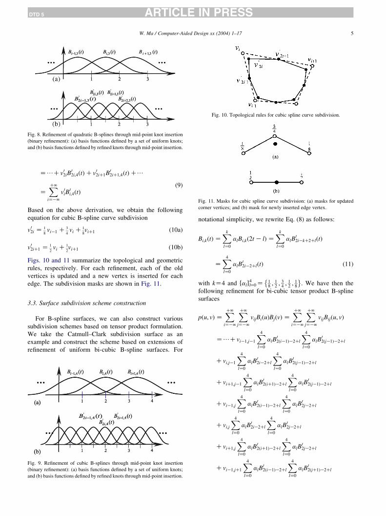
Fig. 10. Topological rules for cubic spline curve subdivision.

Fig. 11. Masks for cubic spline curve subdivision: (a) masks for updated

corner vertices; and (b) mask for newly inserted edge vertex.

Fig. 8. Refinement of quadratic B-splines through mid-point knot insertion

(binary refinement): (a) basis functions defined by a set of uniform knots;

and (b) basis functions defined by refined knots through mid-point insertion.



Z/Cv02iB02i;4ðtÞCv02iC1B0

2iC1;4ðtÞC/

ZXCN

iZKN

v0iB0i;4ðtÞ

(9)

Based on the above derivation, we obtain the following

equation for cubic B-spline curve subdivision

v02i Z 1

8viK1 C 3

4vi C 1

8viC1 (10a)

v02iC1 Z 1

2vi C 1

2viC1 (10b)

Figs. 10 and 11 summarize the topological and geometric

rules, respectively. For each refinement, each of the old

vertices is updated and a new vertex is inserted for each

edge. The subdivision masks are shown in Fig. 11.

3.3. Surface subdivision scheme construction

For B-spline surfaces, we can also construct various

subdivision schemes based on tensor product formulation.

We take the Catmull–Clark subdivision surface as an

example and construct the scheme based on extensions of

refinement of uniform bi-cubic B-spline surfaces. For

Fig. 9. Refinement of cubic B-splines through mid-point knot insertion

(binary refinement): (a) basis functions defined by a set of uniform knots;

and (b) basis functions defined by refined knots through mid-point insertion.

notational simplicity, we rewrite Eq. (8) as follows:

Bi;kðtÞ ZXk

lZ0

alBi;kð2t K lÞ ZXk

lZ0

alB02iKkC2ClðtÞ

ZX4

lZ0

alB02iK2ClðtÞ (11)

with kZ4 and falg4lZ0 Z 1

8; 1

2; 3

4; 1

2; 1

8

�: We have then the

following refinement for bi-cubic tensor product B-spline

surfaces

pðu; vÞ ZXCN

iZKN

XCN

jZKN

vijBiðuÞBjðvÞ ZXCN

iZKN

XCN

jZKN

vijBijðu; vÞ

Z/CviK1;jK1

X4

lZ0

alB02ðiK1ÞK2Cl

X4

lZ0

alB02ðjK1ÞK2Cl

Cvi;jK1

X4

lZ0

alB02iK2Cl

X4

lZ0

alB02ðjK1ÞK2Cl

CviC1;jK1

X4

lZ0

alB02ðiC1ÞK2Cl

X4

lZ0

alB02ðjK1ÞK2Cl

CviK1;j

X4

lZ0

alB02ðiK1ÞK2Cl

X4

lZ0

alB02jK2Cl

Cvi;j

X4

lZ0

alB02iK2Cl

X4

lZ0

alB02jK2Cl

CviC1;j

X4

lZ0

alB02ðiC1ÞK2Cl

X4

lZ0

alB02jK2Cl

CviK1;jC1

X4

lZ0

alB02ðiK1ÞK2Cl

X4

lZ0

alB02ðjC1ÞK2Cl

Fig. 13. Catmull–Clark subdivision masks for quadrilateral meshes: (a)

updated regular V-vertices; (b) updated general V-vertices; (c) newly

inserted F-vertices; and (d) newly inserted E-vertices. In this figure, bnZ3/2n and gnZ1/4n.



Cvi;jC1

X4

lZ0

alB02iK2Cl

X4

lZ0

alB02ðjC1ÞK2Cl

CviC1;jC1

X4

lZ0

alB02ðiC1ÞK2Cl

X4

lZ0

alB02ðjC1ÞK2ClC. ð12Þ

After expanding the terms and reorganization following the

refined basis functions, we obtain

pðu; vÞ ZXCN

iZKN

XCN

jZKN

vijBijðu; vÞ Z/Cv02i;2jB02i;2jðu; vÞ

Cv02iC1;2jB02iC1;2jðu; vÞCv02i;2jC1B0

2i;2jC1ðu; vÞ

Cv02iC1;2jC1B02iC1;2jC1ðu; vÞC/ ð13Þ

where

v02i;2j Z 1

64ðviK1; jK1 C6vi;jK1 CviC1; jK1 C6viK1; j C36vi;j

C6viC1; j CviK1; jC1 C6vi; jC1 CviC1; jC1Þ

v02iC1;2j Z 1

16ðvi; jK1 CviC1; jK1 C6vi; j C6viC1; j Cvi; jC1

CviC1; jC1Þ

v02i;2jC1 Z 1

16ðviK1; j CviK1; jC1 C6vi; j C6vi; jC1 CviC1; j

CviC1; jC1Þ

v02iC1;2 jC1 Z 1

4ðvi; j CviC1;j Cvi; jC1 CviC1; jC1Þ (14)

are the refined control vertices that are defined as a linear

combination of neighboring old vertices. Following

Eq. (14), the refined control vertices can be classified

into three classes as shown in Fig. 12, i.e. newly inserted

Fig. 12. Subdivision of uniform bi-cubic B-spline surfaces. In this figure,

circle vertices are old vertices before refinement, black vertices are newly

updated/inserted vertices after refinement, vertices such as F(2iC1,2jC1)

are newly inserted face vertices (F-vertices), vertices such as V(2i,2j) are

newly updated vertex vertices (V-vertices) of v 02i,2j, and vertices such as

E(2iC7,2j) or E(2i,2jC1) are newly inserted edge vertices (E-vertices).

face vertices (F-vertices) F 02iC1,2jC1Zv 0

2iC1,2jC1,

updated vertex vertices (V-vertices) V2i,2jZv 02i,2j, and

two newly inserted edge vertices (E-vertices) E2iC1,2jZv 0

2iC1,2j and E2i,2jC1Zv 02i,2jC1. Fig. 13(a), (c) and (d)

shows the masks for uniform bi-cubic B-spline surface

subdivision.

To extend the subdivision to general quadrilateral mesh

of arbitrary topology, the refinement of v 02i,2j in Eq. (14) can

be rewritten as

v02i;2j Z 1 K3

8K

1

16

� vi;j C

3=8

4ðvi;jK1 CviK1;j

CviC1;j Cvi;jC1ÞC1=16

4ðviK1;jK1 CviC1;jK1

CviK1;jC1 CviC1;jC1Þ (15)

Now let n be the number of edges incident to vertex vi,

called valence of the corresponding vertex (nZ4 for regular

vertices), bnZ3/2n and gnZ1/4n be two coefficients for

updating the V-vertices (b4Z3/8 and g4Z1/16 for regular

vertices),

fpkgnK1kZ0 Z fvi;jK1; viK1;j; viC1;j; vi;jC1g

be a collection of edge vertices incident to vij, and

fqkgnK1kZ0 Z fviK1;jK1; viC1;jK1; viK1;jC1; viC1;jC1g



be a collection of the opposite corner vertices of vij of faces

incident to vij. The refined control vertices of Eq. (14) can

then written as

v02i;2j Z ð1 Kbn KgnÞvi;j Cbn

n

XnK1

iZ0

pi Cgn

n

!XnK1

iZ0

qi v02iC1;2j

Z1

16ðvi;jK1 CviC1;jK1 C6vi;j C6viC1;j

Cvi;jC1 CviC1;jC1Þ v02i;2jC1

Z1

16ðviK1;j CviK1;jC1 C6vi;j C6vi;jC1

CviC1;j CviC1;jC1Þ v02iC1;2jC1

Z1

4ðvi;j Cvi;jC1 CviC1;j CviC1;jC1Þ (16a)

with the following coefficients

bn Z3

2nand gn Z

1

4n(16b)

Eq. (16) can thus be used for general quadrilateral meshes of

arbitrary topology and it reduces to Eq. (14) for regular

vertices with valence nZ4. This leads to the well-known

Catmull–Clark subdivision for quadrilateral meshes of

arbitrary topology. Fig. 13 shows all related subdivision

masks.

Equation can be further extended to a more general

form for arbitrary control meshes (not just with quad-

rilateral faces). For this purposes, the newly inserted V-

vertex v 02i,2j and E-vertices v 0

2iC1,2j and v 02i,2jC1 of Eq.

(14) can be reorganized based on the newly computed

face vertices

v02i;2j Z ð1 Kb KgÞvi;j Cb

nðvi;jK1 CviK1;j CviC1;j Cvi;jC1Þ

Cg

nðv02iK1;2jK1 Cv02iK1;2jC1 Cv02iC1;2jK1 Cv02iC1;2jC1Þ

v02iC1;2j Z1

4ðvi;j CviC1;j Cv02iC1;2jK1 Cv02iC1;2jC1Þ

v02i;2jC1 Z1

4ðvi;j Cvi;jC1 Cv02iK1;2jC1 Cv02iC1;2jC1Þ ð17aÞ

with the following coefficients

b Z g Z 1=n; (17b)

where, n again stands for the valence of the control mesh

at vertex vij, and

v02iK1;2jK1 Z1

nf

ðviK1;jK1 CviK1;j Cvi;jK1 Cvi;jÞ

v02iK1;2jC1 Z1

nf

ðviK1;j CviK1;jC1 Cvi;j Cvi;jC1Þ

v02iC1;2jK1 Z1

nf

ðvi;jK1 Cvi;j CviC1;jK1 CviC1;jÞ

v02iC1;2jC1 Z1

nf

ðvi;j Cvi;jC1 CviC1;j CviC1;jC1Þ ð17cÞ

are the updated face vertices with nfZ4 being the number

of vertices of the corresponding face. Please note that we

omitted the subscript of b and g in order not to be

confused with Eq. (16), but both the two coefficients vary

depending on the valance n. Now further let

fpkgnK1kZ0 Z fvi;jK1; viK1;j; viC1;j; vi;jC1g

be a collection of edge vertices incident to vij and let

fqkgnK1kZ0 Z fv02iK1;2jK1; v

02iK1;2jC1; v

02iC1;2jK1; v

02iC1;2jC1g

Z fF2iK1;2jK1;F2iK1;2jC1;F2iC1;2jK1;F2iC1;2jC1g

be a collection of newly inserted face vertices (F-vertices)

incident to vertex vij. The refined control vertices of

Eq. (13) can then be represented in yet another form in

terms of newly computed face vertices as:

v02i;2j Z ð1 Kb KgÞvi;j Cb

n

XnK1

iZ0

pi Cg

n

XnK1

iZ0

qi

v02i;2jC1 Z1

4ðvi;j Cvi;jC1 CF2iK1;2jC1 CF2iC1;2jC1Þ

v02iC1;2j Z1

4ðvi;j CviC1;j CF2iC1;2jK1 CF2iC1;2jC1Þ

v02iC1;2jC1 Z1

nf

ðvi;j Cvi;jC1 CviC1;j CviC1;jC1Þ ð18aÞ

with coefficients as follows

b Z g Z 1=n; (18b)

Eq. (18) can now be easily extended to handle arbitrary

control meshes. One can compute newly inserted F-

vertices as an average of all old vertices of the

corresponding face for arbitrary nf and then use Eq. (18)

with a general valence n. This leads to the Catmull–Clark

subdivision in a more general form and can be

summarized as follows:

†
F-vertices: A face vertex for each face is computed as an
average of all old control vertices of the corresponding

face.

†
E-vertices: An edge vertex for each edge is computed as
an average of the two end vertices of the corresponding

edge and the two newly inserted F-vertices whose faces

share the same corresponding edge, i.e. an average of

four related vertices.

†
V-vertices: A vertex vertex is computed as a linear
combination of the corresponding old vertex, all old

Fig. 15. General subdivision masks for Catmull–Clark surfaces: (a) mask

for updated smooth V-vertices and darts; (b) mask for newly inserted E-

vertices; and (c) mask for newly inserted face vertices; (d) mark for updated

crease/boundary V-vertices; and (e) mark for newly inserted crease/bound-

ary E-verices. In this figure, bZgZ1/n and aZ1KbKg (or aCbCgZ1),

and vertices with gray shading are newly inserted face vertices.



vertices incident to the corresponding vertex though

edges, and all newly inserted face vertices whose faces

incident to the corresponding vertex.

The refined V-vertices defined in Eq. (18a) are also often

written in the following explicit form in terms of the valence

n of vij.

v02i;2j Zn K2

nvi;j C

1

n2

XnK1

iZ0

pi C1

n2

XnK1

iZ0

qi (19)

In addition, subdivision rules for sharp feature, such as

crease edges, boundary edges, corners where three or

more creases meet, and darts where a crease edge

terminates, can also be defined. We may keep all corners

unchanged during the refinement (mask not shown in

Fig. 15), use the subdivision rules for cubic curves defined

by Eq.(10) and Figs. 10 and 11 for refining crease and

boundary edges, and use the same mask as that for smooth

vertices for dart vertices. Fig. 14 shows how exactly the

refined control mesh is constructed. Fig. 15 shows the

masks for Catmull–Clark subdivision in case of a general

control mesh.

In case of extraordinary vertices whose valence is

other than 4, i.e. ns4, the coefficients b and g in Eq.

(18) can be selected from a wide range and can be

optimized to achieve well behaved shape at the

extraordinary corner positions. However, it should not

be confused with Eq. (16) in computing V-vertices.

Fig. 16 shows an example of a smooth Catmull–Clark

subdivision surface model.

In a similar way, one may also develop a tensor

product version subdivision scheme for quadratic B-spline

surfaces based on the Chaikin’s algorithm and extend it to

well-known Doo–Sabin subdivision surfaces. In literature,

one may find several other approaches in constructing

various subdivision schemes and in optimizing existing

subdivision schemes for better surface behaviour. In

connection with schemes generalizing B-splines, further

readings can be found in [42,43,47,50,62, and references

therein].

Fig. 14. Topological rules for Catmull–Clark subdivision surfaces.

Fig. 16. Illustration of a Catmull–Clark subdivision surface [6]: (a) the

initial control mesh; (b) the control mesh after one level of refinement; (c)

the control mesh after three refinement; and (d) the limit surface.



4. Overview of subdivision schemes

In literature, one may find rich families of subdivision

schemes. While most of the reported schemes are further

generalizations of a subset of splines [6,10,39,50,62], some

other subdivision schemes are further extensions of box-

splines [22,27,50]. There are also some subdivision schemes

that are discrete versions of other functions, their

analytic version do not exists or are not known at the

moment [11,19,35].

4.1. Key concepts and a brief overview

As discussed in the Section 3, a subdivision scheme is

defined by a set of topological rules and geometric rules for

mesh refinement. Topological rules define how a control

mesh is split into a refined mesh. Depending on the type of a

subdivision scheme, typical operations of topological rules

include insertion of new vertices into edges or faces,

updating of old vertices, connection of newly inserted and

updated vertices (with also old ones if applicable), and

removal of some vertices, edges or faces. Geometric rules

are used to compute the exact coordinates of the refined

Fig. 17. Several important topological subdivision rules (illustrations showing m

subdivision and interpolatoryffiffiffi3

psubdivision [19,20]); (b) 1/4 splitting for D m

paired D meshes (4–8 subdivision [54]); (d) 1/4 splitting for , meshes (Catmull

and interpolatoryffiffiffi2

psubdivision [22,23]); (f) 1/4 splitting for , meshes (D

subdivision [14,36]).

control vertices. When designing geometric rules for mesh

subdivision, key properties need to be considered include

affine invariance, finite support with small subdivision

masks, symmetry, and behaviour of the limit surface.

Techniques for series analysis, such as eigen structure

analysis, z-transformtion and Fourier transformation, are

often used to guide the selection of appropriate subdivision

masks. Fig. 17 summarizes some basic topological rules for

subdividing triangle and quadrilateral meshes. In literature,

one may also find combined schemes that incorporate one or

more of the topological rules summarized in Fig. 17 [35,51,

62]. Fig. 18 shows a Loop subdivision surface that use the

one-to-four splitting topological rule for triangle meshes.

Loop subdivision surfaces are generalizations of three-

directional box-splines and further details about the scheme

can be found in Refs. [16,27]. Fig. 19 shows a pipe model

and a gun model produced using Doo–Sabin and Catmull–

Clark subdivision surfaces, respectively.

In addition, the following is a list of important concepts

in subdivision surface modeling:

†

esh

es

–Cla

oo–

Approximatory versus interpolatory: If the limit surface

of a subdivision scheme does not go through the initial

es before and after subdivision): (a) 1/3 splitting for D meshes (ffiffiffi3

p

hes (Loop and Butterfly subdivision [11,27,60]); (c) 1/2 splitting for

rk subdivision [6,18]); (e) 1/2 splitting for , meshes (ffiffiffi2

psubdivision

Sabin subdivision [10]); (g) 1/2 splitting for , meshes (Midedge

Fig. 18. Illustration of a Loop subdivision surface [27,46]: (a) the initial

control mesh; (b) the control mesh after one level of refinement; (c) the

control mesh after three refinement; and (d) the limit surface.

Fig

defi

init



control points, the subdivision scheme is called an

approximatory subdivision scheme. Examples of approx-

imatory subdivision schemes include Loop subdivision

[27], Doo–Sabin [10] and Catmull–Clark [6] subdivision

. 19. Illustration of a pipe model (a) and (b) and a gun model (c) and (d)

ned as a Doo–Sabin and Catmull–Clark surface, respectively. (a) and (c)

ial control mesh, and (b) and (d) final limit surfaces.

surfaces. Otherwise, the scheme is an interpolatory

subdivision scheme. Typical examples include an

interpolatory Butterfly subdivision [11], Kobbelt sub-

division [18], and an interpolatoryffiffiffi2

psubdivision [23]

and interpolatoryffiffiffi3

psubdivision [20].

†
Stationary versus non-stationary subdivision: If the
subdivision rules do not change during the subdivision

process, the scheme is called a stationary subdivision

scheme and, otherwise, a non-stationary subdivision

scheme. Most of the existing subdivision schemes are

stationary subdivision schemes. To produce certain

classes of shapes, such as a perfect circle, a non-stationary

subdivision scheme may have to be used [17,31].

†
Uniform versus non-uniform subdivision: Most of the
existing subdivision schemes are uniform subdivision

schemes by which an existing mesh is refined

uniformly through mid-point knot insertion over the

entire surface for all levels of subdivision. Otherwise, it

is called a non-uniform subdivision scheme. Most of

the existing subdivision schemes are uniform subdivi-

sion schemes. The NURSS subdivision scheme [47]

can, however, perform parametrized and non-uniform

subdivision.

†
Global versus local or adaptive subdivision: Most of the
existing subdivision schemes are only designed to

perform global subdivision. In certain situations, a

local and adaptive subdivision might be desirable [32,

48]. However, there are no existing subdivision schemes

that can do adaptive subdivision without affecting the

limit surface.

Many of the existing subdivision schemes can handle

sharp features, such as crease and boundary edges [5,14,46,

47]. Sharp features can be classified according to the

number of vertices meeting at a vertex and the type of a

vertex or an edge.

†
Edge classification: We may distinguish three types of
patch boundaries, i.e. an internal smooth edge where the

limit surface is at least C1, a crease edge where the limit

surface is C0, and a boundary edge where the surface

terminates.

†
Vertex classification: Let s be the number of crease edges
meeting at a vertex. One can classify vertices into the

following types according to the number of meeting

crease edges s of the corresponding vertex.

† A smooth vertex where the limit surface is at least C1

has no meeting crease edge with sZ0.

† A sharp vertex has no meeting crease edge with sZ0,

but the limit surface is not smooth at the vertex

position. If the directional tangent of the limit surface

at the vertex position does not vanish, the vertex is

classified as a cone-type vertex. Otherwise, if

the directional tangents of the limit surface at the

vertex position vanish to a single vector, it is classified

as a cusp vertex.

Fig

two

two

me

sur



† A dart vertex is one where a crease edge terminates

with sZ1.

† A crease or boundary vertex is located on a crease or

boundary edge, respectively, with sZ2. A boundary

vertex may also be defined as a corner vertex if the

boundary curve is C0 and the surface goes through

that vertex.

† A corner vertex has sR3.

. 20

dif

clo

sh, b

face

When handling sharp features, such as those for

Catmull–Clark surfaces defined by the masks of Fig. 15(d)

and (e), special rules need to be defined. Fig. 20 highlights

some of the above mentioned crease features. In literature,

one may find rich classes of subdivision rules for defining

crease features for schemes, such as Loop, Doo–Sabin,

Catmull–Clark subdivision schemes and NURSS [5,9,16,

34,46,47]. Most of the other schemes also have various

ready definitions for commonly used crease features.

4.2. Properties of subdivision schemes

The analysis of subdivision surfaces at extraordinary

corner or patch positions differ from that for regular parts of

the control mesh. The later can often be deduced from the

theory of the counter part of the scheme in continuous space,

if available. For Catmull–Clark surfaces, e.g. the properties

. Illustration of sharp features: (a) a smooth model without any sharp feature

ferent views; (d) a model with a closed crease edge and one cusp; (e) a mod

sed boundary edges, four internal crease edges, four darts and four externa

ut marked with different sharp features. Illustrations (a)–(c) are produced w

s.

and continuity conditions of the limit surface on domains of

regular grid of control points can be deduced from cubic B-

spline surfaces, which is C2 continuous. Otherwise, limit

surface properties can be analyzed using the same

techniques as that for the analysis at extraordinary corner

positions [2,8,12]. At extraordinary corner positions,

properties of the limit surface can be studied using various

tools for series analysis, such as z-transformation, Fourier

transformation, and direct eigen structure analysis of the

subdivision matrix of a small invariant stencil, i.e. a subset

of the control mesh, of the corresponding subdivision

scheme. The analysis of subdivision schemes near extra-

ordinary corner positions was first addressed by Doo and

Sabin in Ref. [10]. The properties were then studied by Ball

and Storry in Refs. [1,2] and by Sabin in [41]. Further

investigations were also carried out by Reif in Ref. [40] and

Peters and Reif in Ref. [37]. One may also find some recent

studies, such as [8,38,53,58,59]. At the moment, an elegant

theoretical foundation has been established for the analysis

of various properties, such as continuity conditions and

surface interrogations of subdivision surfaces.

We again use Catmull–Clark surface to illustrate how

the subdivision matrix can be set up and used for limit

surface analysis, but the approach is the same for all

stationary subdivision schemes. Fig. 21(a) shows the

smallest invariant stencil (before and after subdivision) for

s; (b) and (c) a model with two crease edges, four darts and one conical tip in

el with four crease edges, four darts and one corner; (f) an open surface with

l corners. In these illustrations, (a)–(e) are produced with the same control

ith Loop subdivision surfaces and (d)–(f) are produced with Catmull–Clark

Fig. 21. Important invariant stencils of Catmull–Clark surfaces [15,49,61]:

(a) stencil with m ¼ 2n þ 1 vertices for query and interrogation (one ring

for evaluation) or m ¼ 6n þ 1 vertices for surface property analysis (two

rings for continuity and curvature analysis) at extraordinary corner position

v0; and (b) stencil with KZ2nC8 vertices for defining an extraordinary

corner surface patch. In this figure, the valence of the extraordinary corner

is nZ5.



Catmull–Clark surface property evaluation or analysis at

extraordinary corner position v0. In the limit, this stencil

converges to a point on the limit surface corresponding to

v0. Fig. 21(b) shows another invariant stencil (before and

after subdivision) for defining an extraordinary corner

patch of Catmull–Clark surfaces at v0. This stencil is used

in Section 4.3 in setting up another subdivision matrix for

parametric evaluation of extraordinary corner patches of

Catmull–Clark surfaces.

For surface property evaluation or analysis at vertex/

corner positions, the stencil of Fig. 21(a) is used. Let vjZ½v

j0; v

j1;.; v

jmK1�

T and vjC1Z ½vjC10 ; v

jC11 ;.; v

jC1mK1�

T be a

collection of the control points of the stencil before and

after subdivision, respectively. The subdivision equation

can be defined as

vjC10

vjC11

«

vjC1mK1

2666664

3777775Z S

vj0

vj1

«

vjmK1

2666664

3777775 (20)

or vjC1ZSvj in short, with S being the subdivision matrix.

Various properties of the limit surface at v0 can be

determined through direct eigen structure analysis of the

subdivision matrix S. The eigen analysis of the subdivi-

sion matrix, in turn, is also critical for designing well

behaved subdivision masks, i.e. to carefully select

subdivision masks and coefficients that lead to desired

eigen structures and consequently well-behaved surface

properties.

Let us now assume that the subdivision matrix S has

eigen values {l0,l1,.,lmK1} and corresponding left eigen

vectors {x0,x1,.xm-1}, respectively, with eigen values

organized in decreasing moduli jlijR jliC1j: The following

summarizes some important properties of subdivision

surfaces in relation to the eigen structure of the subdivision

matrix [15,40,46,51,58,59]:

†
Affine invariance: The subdivision scheme is affine
invariant if and only if

l0 Z 1: (21)

†
Convergence: A subdivision scheme converges if and
only if 1Zl0Ol1. Otherwise, the subdivision scheme

would diverge if l0O1 and the control point/mesh would

shrink to the origin if l0!1.

†
C1 continuity: The corresponding limit position of the
control vertex v0 is C1 continuous provided that (a) the

characteristic map of the subdivision is regular and

injective, and (b) the sub-dominant eigenvalues satisfy

1 Z l0Ol1Pl2 Ol3/ (22a)

or preferably the following for binary subdivision

schemes

1 Z l0O1

2Z l1 Z l2 Ol3 /: (22b)

†
Bounded curvature: The quality of curvature can be
evaluated by

r Z l3=l21: (23)

In case r!1, one obtains flat/zero curvature. In case

rO1, the curvature would diverge. Only in case rZ1,

one achieves bounded curvature. For well behaved

binary subdivision surfaces, e.g., the sub-dominant

eigenvalue should satisfy

1 Zl0O1

2Zl1 Zl2O

1

4Zl3 Zl4 Zl5Ol6/ (24)

for obtaining bounded curvature at the limit position.

†
Query and interrogation: The corresponding limit
position of a control vertex v0 is defined by

vN0 Z xT

0 v0: (25)

The tangent vectors at the limit position are defined by

c1 Z xT1 v0 and c2 Z xT

2 v0: (26)

The surface normal is defined by

n Z c1 !c2: (27)

The characteristic map of an n-valence vertex is

defined as the planar limit surface whose initial control

net is defined by the two right eigenvectors corresponding

to the two subdominat eigenvalues l1 and l2, respectively

[40,46,59]. For constructing the characterstic map, one

may use a larger stencil for setting up the subdivision

matrix, usually with one more ring control points than

the smallest invariant stencil for analysis. Note that

most of the subdivision schemes, such as the original

Catmull–Clark surfaces discussed in Section 3, only

achieve C1 continuity at extraordinary corner positions.



4.3. Parametric evaluation

Following the discussions of Section 4.2, it is possible to

evaluate the corresponding limit position, the tangent

vectors and surface normal of a control vertex at any

resolution in a single step. In addition, there also exists an

explicit analytical form for parametric evaluation of

subdivision surfaces at an arbitrary position without going

through the process of infinitive subdivision. Following the

derivation reported in Ref. [49] for Catmull–Clark surfaces,

such a parametric evaluation exists for all stationary

subdivision schemes whose regular parts are extensions of

a known form in the continuous domain, which is true for

most of the existing subdivision schemes found in literature.

Although it has not be reported till the moment, some kind

of parametric evaluation might also exist for other

stationary and non-stationary subdivision schemes and

might be derived based on the analysis of the subdivision

scheme through various approaches for analyzing the

subdivision series.

Let us take the Catmull–Clark surface [49] as an

example. For regular patches, the surface can be evaluated

based on uniform bi-cubic B-spline surfaces as follows:

pðu; vÞ ZX15

iZ0

viBiðu; vÞ (28)

where

fBiðu; vÞg15iZ0 Z ffBiðuÞBjðvÞg

3jZ0g

3iZ0

are the usual basis functions for uniform cubic B-spline

surfaces. For extraordinary corner patches, such as the

shaded patch of the initial control mesh shown in Fig. 21(b),

the parametric form for surface evaluation is similar to Eq.

(28) with another set of basis functions fjiðu; vÞgKK1iZ0 as

follows:

pðu; vÞ ZXKK1

iZ0

vijiðu; vÞ (29)

where KZ2nC8 is the total number of control points for

defining an extraordinary corner patch with valance n. The

basis functions fjiðu; vÞgKK1iZ0 of Eq. (29) can be derived

following the eigen structure analysis of a subdivision

matrix defined by the stencil shown in Fig. 21(b) and

further details can be found in Refs. [29,49].

5. Subdivision surface fitting

In literature, one can also find various approaches for

fitting subdivision surfaces to range or scanning data.

Among others, Hoppe et al. [16] presented an approach for

automatically fitting subdivision surfaces from a dense

triangle mesh. Following the fitting criterion, the final fitted

control mesh after two subdivisions will be the closest to

the initial dense mesh, which provides sufficient approxi-

mation for practical applications. Both smooth and sharp

models can be handled. This approach produces high quality

visual models.

The method of Suzuki et al. [52] for subdivision

surface fitting starts from an interactively defined initial

control mesh. For each of the control vertices, the

corresponding limit position is obtained from the initial

dense mesh. The final positions of the control vertices are

then inversely solved following the relationship between

the control vertices and the corresponding limit positions.

The fitted subdivision surface is checked against a pre-

defined tolerance. In case of need, the topological

structure of the control mesh is further subdivided and a

refined mesh of limit positions is obtained. A new

subdivision surface is then fitted from the corresponding

refined limit positions. The procedure is repeated until the

fitted subdivision surface meets the allowed tolerance

bound. The fitting criterion ensures that the resulting

subdivision surface interpolates the corresponding limit

positions of the current control mesh. Since only a subset

of vertices of the initial dense mesh is involved in the

fitting procedure, the computing speed is extremely fast.

Ma and Zhao [28,29] also reported a parametrization-

based approach for fitting Catmull–Clark subdivision

surfaces. A network of global boundary curves is first

interactively defined for topological modeling. A set of base

surfaces is then defined from the topological model for

sample data parametrization. A set of observation equations

is obtained based on ordinary B-splines for regular surface

patches and an evaluation scheme of Stam [49] for

extraordinary surface patches. A Catmull–Clark surface is

finally obtained through linear least squares fitting. The

approach makes use of all known sample points and the

fitting criterion ensures best fitting condition between the

input data and the final fitted subdivision surface. Apart

from the parametrization procedure, the fitting process alone

is pretty fast.

In a recent paper, Ma et al. [30] proposed a direct

method for subdivision surface fitting from a known dense

triangle mesh. A feature- and topology-preserving mesh

simplification algorithm is first used for topological

modeling and a direct fitting approach is developed for

subdivision surface fitting. For setting up the fitting

equations, both subdivision rules and limit position

evaluation masks are used. The final subdivision surface

best fits a subset of vertices of the initial control mesh and

is obtained through linear least squares fitting without any

constraints. Sharp features are also preserved during the

fitting procedure. Further work with improved fitting

results can also be found in [24]. While only a modified

Loop subdivision scheme [27] was discussed in these

papers, the algorithm can be applied to all stationary

subdivision schemes. The processing time is also

extremely fast.

Fig. 22. A paramatrization-based approach for subdivision surface fitting [28,29]: (a) and (b) a vacuum cleaner model; (c) and (d) a piece of femur bone model;

(a) and (c) original contours measured on a medical CT-scanner with extended interpolation points; (b) and (d) final fitted subdivision surface with control

points.



All the above fitting approaches are built upon schemes

for limit surface query, either at discrete positions [16,30,

52] or at arbitrary parameters [28,29]. In literature, one can

also find schemes interpolating a set of surface limit

positions with or without surface normal vectors instead

of fitting conditions [15,34]. In theory, all interpolation

schemes can be extended as a fitting scheme if the number

of known surface conditions, such as limit positions, normal

vectors and other constraints, is more than that of the

unknown control vertices of the subdivision surface. Several

authors [3,44,45] also explored reversal of Loop, Butterfly

and the original Doo subdivisions through wavelets analysis

and least squares fitting. Lee et al. [21] also proposed an

approach for surface reconstruction, called a displaced

subdivision surface, from an arbitrary triangle mesh with

details. The displaced subdivision surface is defined as a

smooth subdivision surface with a scalar-valued displace-

ment map applied to the limit positions of a refined control

mesh. The smooth subdivision surface was obtained through

mesh simplification. Guskov et al. [13] also constructed a

normal mesh with wavelets coefficients as hierarchical

displacements applied to a multi-resolution mesh. The

normal mesh can be considered as a kind of generalization

of the displaced subdivision surfaces of Lee et al. [21]. One

can also find an approach for adaptively fitting a Catmull–

Clark subdivision surface to a given shape through a fast

local adaptation procedure [26]. The fitting process starts

from an initial approximate generic model defined as a

subdivision surface of the same type.

Fig. 22 shows two fitting examples produced using the

paramatrization based approach for subdivision surface

fitting [28,29]. The original data for both of these models

were measured using CT-scanners. Fig. 22(a) and (c) shows

the original measured CT contours with superposed

interpolation points. Fig. 22(b) and (d) show the final fitted

Catmull–Clark surfaces. Further details regarding the fitting

approach can be found in Refs. [28,29]. Fig. 23 shows two

fitting examples produced using the direct approach for

subdivision surface fitting [24,30]. Fig. 23(a) and (d) on the

left are input triangle meshes. Fig. 23(b) and (e) in the

middle are control meshes of the fitted Loop subdivision

surface. Fig. 23(c) and (f) present the final fitted Loop

subdivision surface. Further details regarding the fitting

approach can be found in Refs. [24,30].

The above examples also demonstrate the modeling

capability of subdivision surfaces. If one had used

traditional B-splines, one would have had to maintain

the continuity among individual surfaces, which is an

extremely difficult task for today’s CAD systems. Even if

one can represent the entire model as a mosaic of B-

spline surfaces with continuity conditions, it is still not

possible to modify the surface by moving a control

points near domain boundaries, or one breaks all the

continuity conditions. With subdivision surfaces, how-

ever, the continuity conditions along all patch boundaries

are automatically maintained. One can modify the shape

by moving any of its control points, just like manipulat-

ing the control points of a single B-spline surface.

While many approaches have been reported so far,

several other important areas may be further explored. On

topological modeling, adaptive approaches and techniques

for arbitrary mesh processing can be further studied.

Fig. 23. A direct approach for automatic subdivision surface fitting [24,30]: (a)–(c) a test part with marked sharp features; (d)–(f) a mannequin model; (a) and

(d) original triangle mesh; (b) and (e) control mesh of the fitted Loop subdivision surfaces; (c) and (f) final fitted Loop subdivision surfaces.



On stationary subdivision surface fitting, elaborated pro-

cedures may be developed to further handle fitting with

various given constraints, such as known limit positions,

local tangents and surface normal vectors. Local piecewise

fitting procedures and adaptive approaches may also be

further developed for parallel processing of extremely large

surface meshes. Techniques for fitting non-stationary and

other subdivision surfaces also need to be developed.

6. Other topics in subdivision surface modelling

During the past decade or so, subdivision surfaces have

received extensive attention in free-form surface modelling,

multi-resolution representation, and computer graphics.

Families of new subdivision schemes were proposed, many

new theoretical tools were developed, and various practical

results were obtained. Recently, several other topics have

also attracted enormous attention and there is a lot of space

for further development in many other topics.

†
Unified subdivision schemes and standardization: One of
the topics addressed in recent years is the pursuit of unified

subdivision schemes [31,35,50,55,57,62], an important

step towards wide practical applications. Ultimately a

further unified generalization like NURBS for the CAD

and graphics community and further standardization are

expected. Such a unified generalization should cover all

what we can do with NURBS, including the exact

definition of regular shapes such as sphere, cylinder, cone,

and various general conical shapes and rotational

geometry.

†
Continuity conditions at extraordinary corner positions:
Another topic is the lifting of continuity conditions at

extraordinary corner positions in handling general

degrees that should be the same as that for regular part

of subdivision surfaces. While we are striving to seek

subdivision schemes with small masks for simplicity, it

should be acceptable as long as it is easy to implement,

such as repeated averaging for generalizing high order B-

splines [50,62].

†
Manipulation tools: For wide practical use, advanced
manipulation tools, such as trimming, intersection, off-

setting, Boolean operations, visual effects must be

developed. While there have be various attempts [4,25,

33], there is significant space for further development in

these areas.

†
Other topics: Other important topics include further
development in surface fitting and interpolation, faring

subdivision surface generation, subdivision surface mod-

eling from curve nets, mass property evaluation, geometry

compression, interfacing issues and compatibility with

existing parametric surface software, adaptive subdivi-

sion algorithms that lead to the same limit surface.

One may find further discussions in Refs. [42,43,56,61]

regarding the above and some other topics on subdivision

based modeling.



7. Conclusions

Similar to spline surfaces, subdivision surfaces are

defined by a set of control points. Instead of explicit

parametrization for defining B-spline surfaces, the para-

metrization of a subdivision surface is implicitly defined

by its subdivision rules, i.e. topological rules for mesh

refinement and geometric rules for computing vertices of

refined meshes. While a subdivision surface is defined as

the limit of recursive subdivision and refinement,

algorithms for explicit parametric evaluation of subdivi-

sion surfaces in a single step may also be developed.

Such a parametric evaluation has been reported for

Catmull–Clark and Loop surfaces, but the technique can

be applied to any stationary subdivision schemes whose

parametric form exists for regular part of the surface. It

might also be possible to develop an explicit form for

parametric evaluation of other subdivision schemes

through the analysis of the subdivision series for some

other subdivision schemes. The most important merit of

subdivision surfaces for the CAD and graphics commu-

nity is the ability in handling control meshes of arbitrary

topology. In addition, subdivision algorithms, if

implemented properly, can form the basis for a wide

range of extremely fast and robust interrogations. In

literature, many subdivision schemes and elegant theor-

etical tools have been developed. Many other areas have

been addressed and can be further developed, especially

on unified subdivision schemes that is capable of

generalizing the entire family of NURBS, the current

de-facto standard for CAD and graphics. Many other

algorithms for subdivision surface manipulation should

also be developed for wide engineering applications.

Acknowledgements

The work presented in this paper was supported by City

University of Hong Kong through a Strategic research Grant

(7001296) and by the Research Grants Council of Hong

Kong through a CERG research grant (CityU 1131/03E).

The control mesh of the gun model shown in Fig. 19(c) was

downloaded from http://www.elysium.co.jp/3dtiger/en/

download/ Special thanks also go to N. Zhao, G. Li and Z.

Wu for the implementation of several subdivision schemes

at CityU.

References

[1] Ball AA, Storry DJT. Recursively generated B-spline surfaces. Proc

CAD 1984;84:112–9.

[2] Ball AA, Storry DJT. Conditions for tangent plane continuity over

recursively generated B-spline surfaces. ACM Trans Graph 1988;

7(2):83–102.

[3] Bartels R, Samavati F. Reverse subdivision rules: local linear

conditions and observations on inner products. J Comput Appl Math

2000;119:29–67.

[4] Biermann H, Kristjansson D, Zorin D. Approximate Boolean

operations on free-form solids. Proceedings of ACM SIGGRAPH

computer graphics 2001 p. 185–94.

[5] Biermann H, Martin I, Zorin D, Bernardini F. Sharp features on

multiresolution subdivision surfaces. Graph Models 2002;64(2):

61–77.

[6] Catmull E, Clark J. Recursively generated B-spline surfaces on

arbitrary topological meshes. Comput Aided Des 1978;10:350–5.

[7] Chaikin G. An algorithm for high-speed curve generation. Comput

Graph Image Process 1974;3:346–9.

[8] Daubechies I, Guskov I, Sweldens W. Regularity of irregular

subdivision. Constr Approx 1999;15(3):381–426.

[9] DeRose T, Kass M, Truong T. Subdivision surfaces in character

animation. In: Proceedings of ACM SIGGRAPH computer graphics,

1998. p. 85–94.

[10] Doo D, Sabin M. Behaviors of recursive division surfaces near

extraordinary points. Comput Aided Des 1978;10:356–60.

[11] Dyn N, Levin D, Gregory JA. A butterfly subdivision scheme for

surface interpolation with tension control. ACM Trans Graph 1990;

9(2):160–9.

[12] Dyn N. Subdivision schemes in computer aided geometric design. In:

Light WA, editor. Advances in numerical analysis II, subdivision

algorithms and radial functions. Oxford: Oxford University Press;

1992. p. 36–104.

[13] Guskov I, Vidimce K, Sweldens W, Schroder P. Normal meshes.

Proceedings of ACM SIGGRAPH computer graphics July 2000 p. 95–

102.

[14] Habib A, Warren J. Edge and vertex insertion for a class of

C1 subdivision surfaces. Comput Aided Geom Des 1999;16:

223–47.

[15] Halstead M, Kass M, DeRose T. Efficient fair interpolation using

Catmull–Clark surfaces. Proceedings of the ACM SIGGRAPH


[16] Hoppe H, DeRose T, Duchamp T, Halstead M, Jin H, McDonald J,

Schweitzer J, Stuetzle W. Piecewise smooth surface reconstruction.

Proceedings of the ACM SIGGRAPH computer graphics 1994 p.

295–302.

[17] Jena MK, Shunmugaraj P, Das PC. A non-stationary subdivision

scheme for generalizing trigonometric spline surfaces to arbitrary

meshes. Comput Aided Geom Des 2003;20:61–77.

[18] Kobbelt L. Interpolatory subdivision on open quadrilateral nets with

arbitrary topology. Proceedings of eurographics 96, computer

graphics forum 1996 p. 409–20.

[19] Kobbelt L.ffiffiffi3

p-subdivision. Proceedings of ACM SIGGRAPH


[20] Labisk U, Greiner G. Interpolatoryffiffiffi3

p-subdivision. Comput Graph

Forum (EUROGRAPHICS 2000) 2000;19(3):131–8.

[21] Lee A, Moreton H, Hoppe H. Displaced subdivision surfaces.

Proceedings of the ACM SIGGRAPH computer graphics July 2000

p. 85–94.

[22] Li G, Ma W, Bao H.ffiffiffi2

pSubdivision for quadrilateral meshes. Vis

Comput 2004;20(2–3):180–98.

[23] Li G, Ma W, Bao H. Interpolatoryffiffiffi2

p-subdivision surfaces.

Proceedings of GMP : geometric modelling and processing—

theory and applications. California: IEEE Computer Press; 2004 p.

185–94.

[24] Li G, Ma W, Bao H. A system for subdivision surface fitting.

J Comput Aided Des Comput Graph 2004 [preprint].

[25] Litke N, Levin A, Schroder P. Trimming for subdivision surfaces.

Comput Aided Geom Des 2001;18:463–81.

[26] Litke N, Levin A, Schroder P. Fitting subdivision surfaces.

Proceedings of scientific visualization 2001 p. 319–24.

[27] Loop C, Smooth subdivision surfaces based on triangles, Master’s

Thesis, Department of Mathematics, University of Utah; 1987.

http://www.cse.Ohio-state.edu/(raghu/Papers/cagd_wu.pdf




[28] Ma W, Zhao N. Catmull–Clark surface fitting for reverse engineering

applications. Proceedings of GMP: geometric modelling and

proccesing—theories and applications. California: IEEE Computer

Society; 2000 p. 174–283.

[29] Ma W, Zhao N. Smooth multiple B-spline surface fitting with

Catmull–Clark surfaces for extraordinary corner patches. Vis Comput

2002;18(7):415–36.

[30] Ma W, Ma X, Tso S-K, Pan ZG. A direct approach for subdivision

surface fitting from a dense triangle mesh. Comput Aided Des 2004;

36(6):525–36.

[31] Morin G, Warren J, Weimer H. A subdivision scheme for surfaces of

revolution. Comput Aided Geom Des 2001;18:483–502.

[32] Muller H, Jaeschke R. Adaptive subdivision curves and surfaces.

Computer graphics International 1998, June 22—26, 1998, Hannover,

Germany, IEEE Computer 1998 p. 48–58.

[33] Nasri AH. Interpolating meshes of boundary intersecting curves by

subdivision surfaces. Visual Comput 2000;16(1):3–14.

[34] Nasri A, Sabin M. Taxonomy of interpolation constraints on recursive

subdivision surfaces. Vis Comput J 2002;18(6):382–403.

[35] Oswald P, Schroder P. Composite primal/dualffiffiffi3

p-subdivision

schemes. Comput Aided Geom Des 2003;20(2):135–64.

[36] Peters P, Reif U. The simplest subdivision scheme for smoothing

polyhedra. ACM Trans Graph 1997;16(4):420–31.

[37] Peters J, Reif U. Analysis of algorithms generalizing B-spline

subdivision. SIAM J Numer Anal 1998;35(2):728–48.

[38] Prautzsch H. Smoothness of subdivision surfaces at extraordinary

points. Adv Comp Math 1998;14:377–90.

[39] Prautzsch H, Umlauf G. A G2 subdivision algorithm. In:

Farin G, Bieri H, Brunnett G, DeRose T, editors. Geometric

modelling, computing suppl, vol. 13. Berlin: Springer; 1998. p.

217–24 p. 217–24.

[40] Reif U. A unified approach to subdivision algorithms

near extraordinary vertices. Comput Aided Geom Des 1995;12(2):

153–74.

[41] Sabin MA. Cubic recursive division with bounded curvature. In:

Laurent PJ, Mehaute A, Schu-maker LL, editors. Curves and surfaces.

Academic Press; 1991 p. 411–4.

[42] Sabin MA. Subdivision surfaces. In: Farin GE, Hoschek J, Kim MS,

editors. Handbook of computer aided geometric design. New York:

North Holland; 2002. p. 309–25.

[43] Sabin MA. Recent progress in subdivision—a survey. In: Dodgson N,

Floaterand MS, Sabin M, editors. Advances in multiresolution for

geometric modelling. Berlin: Springer; 2004.

[44] Samavati F, Bartels R. Multiresolution curve and surface represen-

tation: reversing subdivision rules by least squares data fitting.

Comput Graph Forum 1999;18:97–119.

[45] Samavati F, Mahdavi-Amiri N, Bartels R. Multiresolution surfaces

having arbitrary topology by a reverse Doo subdivision method.

Comput Graph Forum 2002;21:121–36.

[46] Schweitizer JE. Analysis and application of subdivision surfaces. PhD

Thesis. Seattle, WA: University of Abhijit; 1996.

[47] Sederberg TW, Zheng J, Sewell D, Sabin M. Non-uniform recursive

subdivision surfaces. Proceedings of the ACM SIGGRAPH computer

graphics 1998 p. 387–94.

[48] Sovakar A, Kobbelt L, . API design for adaptive subdivision schemes.

Comput Graph 2004;24:67–72.

[49] Stam J. Exact evaluation of Catmull–Clark subdivision surfaces at

arbitrary parameter values. Proceedings of the ACM SIGGRAPH


[50] Stam J. On subdivision schemes generalizing uniform B-spline

surfaces of arbitrary degree. Comput Aided Geom Des 2001;18(5):

383–96.

[51] Stam J, Loop C. Quad/triangle subdivision. Comput Graph Forum

2003;22(1):1–7.

[52] Suzuki H, Takeuchi S, Kanai T, Kimura F. Subdivision surface fitting

to a range points. Proceedings of the seventh Pacific graphics

international conference 1999 p. 158–67.

[53] Umlauf G. Analyzing the characteristic map of triangular subdivision

schemes. Constr Approx 2000;16(1):145–55.

[54] Velho L, Zorin D. 4–8 Subdivision. Comput Aided Geom Des, Spec

Issue Subdivision Tech 2001;18(5):397–427.

[55] Warren J, Schaefer S. A factored approach to subdivision surfaces.

Comput Graph Appl 2004;24(3):74–81.

[56] Warren J, Weimer H. Subdivision methods for geometric design.

Subdivision methods for geometric design, a constructive approach.

Boston: Morgan Kaufmann Publishers; 2002.

[57] Wu X, Thompson D, Machiraju R. A generalized corner-cutting

subdivision scheme. http://www.cse.Ohio-state.edu/(raghu/Papers/

cagd_wu.pdf; 2002.

[58] Zorin D. Smoothness of stationary subdivision on irregular meshes.

Constr Approx 2000;16(3):359–97.

[59] Zorin D. A method for analysis of C1-continuity of subdivision

surfaces, SIAM. J Numer Anal 2000;37(5):1677–708.

[60] Zorin D, Schroder P, Sweldens W. Interpolating subdivision for

meshes with arbitrary topology. Proceedings of the ACM SIGGRAPH


[61] Zorin D, Schroder P. Subdivision for modeling and animation. ACM

SIGGRAPH Course Notes, New Orleans, July 23–28 2000.

[62] Zorin D, Schroder P. A unified framework for primal/dual

quadrilateral subdivision scheme. Comput Aided Geom Des 2001;

18(5):429–54.

Weiyin Ma is an Associate Professor in

manufacturing engineering at the City Univer-

sity of Hong Kong (CityU). He lectures in the

areas of geometric modeling, CAD/CAM and

rapid prototyping. His present research inter-

ests include computer aided geometric design,

CAD/CAM, virtual design and virtual manu-

facturing, rapid prototyping and reverse engin-

eering. Prior to joining CityU, he worked as a

research fellow at Materialise N.V., a rapid

prototyping firm in Belgium. He also worked

in the Department of Mechanical Engineering of Katholieke Universiteit

Leuven (K.U. Leuven), Belgium, and the Department of Space Vehicle

Engineering of East China Institute of Technology (ECIT), China. He

obtained a BSc in 1982 and an MSc in 1985 from ECIT, an MEng in 1989

and a PhD in 1994 from K.U. Leuven.



Documents

ARTICLE IN PRESSkowon.dongseo.ac.kr/~lbg/web_lecture/grapprog/20122/... · 2015-02-06 · Subdivision surfaces refer to a class of modelling schemes that deﬁne an object through