Article Effective Intrusion Detection System using XGBoost · and others. XGBoost is employed on the NSL-KDD dataset to get the desired results. The whole motive is to learn about

Information 2017, 8, x; doi: FOR PEER REVIEW www.mdpi.com/journal/information

Article

Effective Intrusion Detection System using XGBoost

Sukhpreet Singh Dhaliwal 1,*, Abdullah-Al Nahid 1, Robert Abbas 1

1 [email protected], 1 [email protected], 1 [email protected]

1 Macquarie University, Sydney, Australia. * Correspondence: [email protected]

Abstract: As the world is on the verge of venturing into fifth-generation communication technology

and embracing concepts such as virtualization and cloudification, the most crucial aspect remains

“security”, as more and more data gets attached to the internet. This paper reflects a model designed

to measure the various parameters of data in a network such as accuracy, precision, confusion matrix

and others. XGBoost is employed on the NSL-KDD dataset to get the desired results. The whole

motive is to learn about the integrity of data and have a higher accuracy in the prediction of data. By

doing so the amount of mischievous data floating in a network can be minimized, making the

network a secure place to share information. The more secure a network is, the fewer situations when

data is hacked or modified. By changing various parameters of the model, future research can be

done to get the most out of the data entering and leaving a network. The most important player in

the network is data and getting to know it more closely and precisely is half the work done. Studying

data in a network and analyzing the pattern and volume of data leads to the emergence of a solid

Intrusion Detection System, that keeps the network healthy and a safe place to share confidential

information.

Keywords: Classifiers; eXtreme Gradient Boosting (XGBoost); Intrusion Detection System (IDS);

Network Socket Layer - Knowledge Discovery in Databases (NSL-KDD).

________________________________________________________________________________________

1. Introduction

One of the most important needs in life is security, whether in normal day-to-day life or in

the cloud world. The year 2017 witnessed a series of ransomware attacks (a simple form of malware

that locks down computer files using strong encryption, and then hackers ask for money in exchange

for release of the compromised files), targets including San Francisco’s light-rail network, Britain’s

National Health Service, and even companies such as FedEx. One example is the WannaCry

Ransomware Attack which compromised thousands of computers, and lately companies such as

Amazon, Google, IBM have started hiring the best minds in digital security so that their

establishments across the world do not get easily compromised. Moreover, one can ask Amazon,

Twitter, Netflix and others about the Denial of Service attacks their servers faced back in 2016 [1], in

which the attackers flooded the system with useless packets, making the system unavailable. There

were virtual machine escape attacks reported back in 2008 by Core Security Technologies, in which a

vulnerability (CVE-20080923) was found in VMware’s (software developing firm named VMware

Inc.) mechanism of shared folders, which made escape possible on VMWare’s Workstation 6.0.2 and

5.5.4 [2]. The virtual-machine escape is a process of escaping the gravity of a virtual machine (isolated

guest operating system) and then communicating with the host operating system. This can lead to a

lot of security hazards. Attackers find new ways to exploit the network, and the security handlers

need to be one step ahead by plugging all leakages beforehand. Many organizations are specially

dedicated to come up with a security architecture that is robust enough to be employed in a clouding

Information 2017, 8, x FOR PEER REVIEW 2 of 28

environment. Cato Networks (Israel), Cipher Cloud (San Jose, California), Cisco Security (San Jose,

California), Dell Security (Texas) [3], Hytrust (California) are some of the organisations that are built

with the sole purpose of making the cloud environment a safe place. Various researchers have put a

lot of work into the field of cloud security and have proposed Intrusion Detection Systems (IDS) as a

solid approach to tackle the issue of security. What an IDS does is that it captures and monitors the

traffic and system logs across the network, and also scans the whole network to detect suspicious

activities. Anywhere the IDS sees a vulnerability, it alerts the system or the cloud administrator about

the possible attack. IDSs are placed at different locations in a network; if placed at the host, they are

termed host-based IDSs (HIDS), while those placed at network points such as gateways and routers

are referred to as Network based IDSs (NIDS). One employed at the Hyper-Visor (or VMM – Virtual

Machine Monitor) is called the Hyper-Visor based IDS (HVIDS). The HIDSs keep an eye on the VMs

running and scan them for suspicious system files, system calls, unwanted configurations and other

irregular activities. The NIDS is basically employed to check for anomalies in the network traffic. The

HVIDS is capable enough to filter out any threats looming over the VMs (Virtual Machines) that are

running over the hypervisor. Some widespread techniques are Misuse detection techniques, in which

already-known attack signatures and machine-learning algorithms are used to find out any mismatch

with the captured data and any irregularities are reported. Similarly, in an anomaly detection the

system matches the behavioral pattern of data coming into the network with a desired behavioral

pattern, and a decision is taken on letting the data flow further into the network or filtering it there

and then. Thus, anomalies are detected. VMI is Virtual Machine Introspection in which programs

running on VMs are scanned and dealt with. The VM introspection can be done in various ways such

as kernel debugging, interrupt based, hyper-call authentication based, guest-OS hook based, VM

state access based. These all ways help to determine whether any suspicious programs are running

at the low-level or high-level semantic end of the VM. There are many tools available such as Ether

[4] (a framework designed to do malware analysis, leveraging hardware virtualization extensions to

remain hidden from malicious software), that help in performing this task from outside the VM. The

traditional IDS techniques were vulnerable as they were basically employed from within the VM, but

with VMI the chances of the VM being attacked are less as the introspection is being done from

outside using VMM technology. The VMM software helps to create and run all VMs attached to it. It

represents itself to attackers as being the targeted VM and prevents direct access to the physical

hardware at the real VM. The VMI technique is employed at the VMM (privileged domain) that helps

to keep an eye on other domains. The catch here is that the hypervisor or VMM itself may be attacked.

For that scenario HVI (Hyper-Visor Introspection) is developed; this depends mainly on hardware

involvement to check the kernel states of the host and hypervisor operating system. Here attacks such

as rootkit, side-channel attacks and hardware attacks can take place.

This paper will present a model through which various parameters related to the data are

calculated, based on which an IDS could be developed to help secure the network. Section 1 offers a

brief introduction to the IDS and data integrity importance, Section 2 discusses the motivation and

reasons to pick up this subject as an area of research, Section 3 covers a literature review related to

the topic which will describe the various methods used to classify data, Section 4 represents the

classification model used to carry out the results, Section 5 offers more theory and background on the

immediate techniques used in this paper, including decision trees, boosting and XGBoost, Section 6

explains the mathematical aspects of XGBoost and how the algorithm works in general, Section 7

presents the main results achieved through the XGBoost algorithm on the NSL-KDD dataset, and

finally Section 8 concludes the paper.

2. Motivation

The main idea that sits behind deploying IDS in a network is to stop attacks happening

from outside and within the network. The findings in this paper can help in building a strong IDS,

which can keep an eye on the data entering a network and simultaneously filter out suspicious

entries. It is recommended that the IDS be deployed at two points. As there is a firewall protecting


the host network or the private network, it is better to place the IDS behind the firewall as seen in

Figure 2.0. Thereby the work of the IDS is reduced and there will be a saving of resources, as the IDS

can only tackle suspicious entries that were unable to be detected by the firewall.

Figure 2.0. Recommended placement of IDS in a network

The IDS deployed can work efficiently and look for suspicious activities within the network.

The main attacks come from outside the host network, from the internet that is trying to send data to

the host network. The main area where this issue can be tackled is the DMZ, that is a demilitarized

zone (the servers that are responsible to connect the host network with the outside world). So, there

can be an IDS that can be deployed endemic to the DMZ and this can help in eliminating the majority

of the mischievous data trying to penetrate the firewall. For more security, a no-access policy should

be assigned to the DMZ servers [5] because, if the DMZ gets compromised, the host network remains

safe. This arrangement of IDS can lead to a more secure network and the machine-learning algorithms

employed within the IDS can help to make the network more secure and intelligent. These IDSs can

be interrogated, and a huge amount of data related to machines can be extracted which can lead to

further studies regarding IoT, Artificial Intelligence, data mining, machine learning and others.

An IDS acts as a sensor, monitoring the network it is employed in. It senses the network for

irregularities and reports them to the network administrator. The best thing that can be done to the

IDS is that the IDS can be used to interact with a mobile phone. The IDS can give regular updates to

the administrator about the network status. It can interact with applications that would want to get

attached to the IDS. The IDS plays a very important role in a network as it monitors the network,


triggers a response to the concerned party when any violation is sensed and, through machine

learning, adapts itself to new network changes, so eliminating the need for constant updates. It can

be in no sense underestimated what an IDS can achieve in bringing security to a network. The more

developed and interactive the IDS is, the faster the response to any illegal activity.

Moreover, there can be applications specifically developed in the future which sit on your

mobile screen, and one touch could give the IDS status of your network, or even the network your

phone is attached to. This can serve as a signal to the user of a network, how secure is the networking

environment.

The main motivation is to build up a strong classification model that sits within an IDS and

can classify the data entering the network with as much accuracy as possible. This paper provides

results which tell us that XGBoost is very well suited to build up a strong classification model. This

can lead to a strong IDS, and a strong IDS enables the network to be a secure place to share

information.

3. Literature Review

Ektefa [6] compared the C4.5 and SVM (Support Vector Machine) algorithms and, in the

findings represented by him, C4.5 worked better for data classification. Most classifiers are based on

the error rate, so they cannot be extended to multiclass complex real problems. Holden came up with

a hybrid PSO (Particle Swarm Optimization) algorithm to deal with normal attribute values but it

lacked many features [7]. Ardjani used SVM and PSO together to optimize the performance of the

SVM [8]. As the data set used for an IDS is mostly multidimensional in nature, it is important to get

rid of inconsistent and redundant features before extracting the features for classification of data. The

selection of features through genetic algorithms gives a better result than when individually applied.

Panda uses two major classification methods, namely, normal or attack [9]. The combination of RBF

(Gaussian Radial Basis Function) and the J48 algorithm (a type of greedy algorithm based on decision

trees) has a higher RMSE (Root Mean Square Error) rate and is more prone to errors. Compared to

this Random Forest and Nested Dichotomies show a 99% detection rate and an error rate of a mere

0.06%.

Petrussenko Denis used LERAD (Learning Rules for Anomaly Detection) to detect attacks

at the network level by using the network packets and TCP flow to learn about new attack patterns

and the general trend of packet flow [10]. He found that LERAD worked well using the DARPA

(Defence Advanced Research Projects Agency) data set, giving a high detection rate. Mahoney used

the various available anomaly methods like ALAD (Application Layer Anomaly Detector), PHAD

(Packet Header Anomaly Detector), and LERAD (performed the best) to model the application, data-

link and other layers of the model [11]. SNORT (developed by CISCO Systems), which is an open

source IDS (used in collaboration with PHAD and NETAD) [12], tested on the IDEVAL (Intrusion

Detection Evaluation) data set detects up to 146 attacks out of a possible 201 attacks, when monitored

for a week.

The Unsupervised method uses a huge volume of data and has less accuracy. To overcome

this a semi-supervised algorithm is used [13]. Fuzzy Connectedness based Clustering is used using

the properties of clusters such as Euclidean distance and statistics [14]. This helps to detect known

and unknown shapes. Ching Hao used unlabelled data in a co-training framework to better intrusion

detection [15]. Here a low error rate was achieved, which helped in setting up an active learning

method to enhance the performance. The semi-supervised technique is used to filter false alarms and

provides a high detection rate [16].

To improve the accuracy, a Tri Training SVM algorithm is used [17]. Adding further,

Monowar H. Bhuyan used the tree-based algorithm to come up with clusters in the dataset without

the use of labelled data [18]. However, labelling can be done on the data set by using a cluster labelling

technique which is based on the Tree CLUS (clusters) algorithm (works faster for numeric and other

mixed datasets).


The Partially Observable Markov Decision Process was used to determine the cost function

using both the anomaly and misuse-detection methods [19]. The Semi-Supervised technique is then

applied to a set of three different SVM classifiers and to the same PSVM (Principal SVM) classifiers.

DDoS, that is Distributed Denial of Service Attacks are the most difficult to counter, as they

are difficult to detect, but two ways are suggested to tackle them. The first way is to filter the traffic

there and then by eliminating the mischievous traffic beforehand, and the second method is to

gradually degrade the performance of the legitimate traffic. The major reason for the widespread

DDoS attacks is the presence of Denial of Capability attacks. The Sink Tree model helps to eliminate

these attacks [20].

The DDoS attacks are not endemic to a network, but they harm the whole network. Zhang

[23] proposed a proactive algorithm to tackle this problem. Here the network was divided into

clusters, with packets needing permission to enter, exit or pass through other clusters. The IP prefix-

based method is used to control the high-speed traffic and detect the DDoS attacks, which come in a

streaming fashion. There is some suggestion to use acknowledgment-based ways to supress

intrusion. Here the clock rates are synchronized with each other (client and server) and any lack or

delay in the clock rates or acknowledgment loss allows the adversary to cause a direct attack on the

client [21].

Pre-processing the network data consumes time, but classification and labelling of data are

the main challenges encountered in an IDS [22]. Issues such as classification of data, high-level pre-

processing, suppression and mitigation of DDoS attacks, False Alarm Rates, and the Semi-Supervised

Approach need to be dealt with to come up with a strong IDS model, and this paper is a step towards

achieving it. Most of the classification methods discussed above had their own advantages and

limitations, XGBoost was chosen because it helped in tackling majority of the flaws that emerged

from the existing models. The reason XGBoost is handpicked to be the preferred classification model

when dealing with issues encountered in real word classification problems is due to the following

reasons:

• XGBoost is approximately 10 times faster than existing methods on a single platform,

therefore eliminating the issue of time consumption especially when pre-processing of the

network data is done.

• XGBoost has the advantage of parallel processing, that is uses all the cores of the machine it

is running on. Highly scalable, generates billions of examples using distributed or parallel

computation and algorithmic optimization operations, all using minimal resources.

Therefore, is highly effective in dealing with issues such as classification of data and high-

level pre-processing of data.

• The portability of XGBoost makes it available and easier to blend on many platforms.

Recently, the distributed versions are being integrated to cloud platforms such as Tianchi of

Alibaba, AWS, GCE, Azure and others. Therefore, flexibility offered by XGBoost is immense

and is not tied to a specific platform, hence the IDS using XGBoost can be platform

independent, a major advantage. XGBoost is also interfaced with cloud data flow systems

such as Spark and Flink.

• XGBoost can be handled by multiple programming languages such as Java, Python, R, C++.

• XGBoost allows the use of wide variety of computing environments such as parallelization

(tree construction across multiple CPU Cores), Out of core computing, distributed computing

for handling large models, and Cache Optimization for the efficient use of hardware.

• The ability of XGBoost to make a weak learner into a strong learner (boosting) through its

optimization step for every new tree that attaches, allow the classification model to generate

less False Alarms, easy labelling of data and accurate classification of data.

• Regularization is an important aspect of XGBoost algorithm, as it helps in avoiding data

overfitting problems whether it be tree based or linear models. XGBoost deals effectively

with data-overfitting problems, which can help to deal when a system is under DDoS attack,

that is flooding of data entries, so the classifier is needed to be fast (which XGBoost is) and

the classifier should be able to accommodate data entries.


• There is enabled cross validation as an internal function. Therefore, no need of external

packages to get cross validation results.

• XGBoost is well equipped to detect and deal with missing values.

• XGBoost is a flexible classifier as it gives the user the option to set the objective function as

desired by setting the parameters of the model. It also supports user defined evaluation

metrics in addition to dealing with regression, classification and ranking problems.

• Availability of XGBoost at different platforms makes it easy to access and use.

• Save and Reload functions are available, as XGBoost gives the option of saving the data

matrix and relaunching it when required. This eliminates the need of extra memory space.

• Extended Tree Pruning, that is, in normal models the tree pruning stops as soon as a negative

loss is encountered, but in XGBoost the Tree Pruning is done up to a maximum depth of tree

as defined by the user and then backward pruning is performed on the same tree until the

improvement in the loss function is below a set threshold value.

All these important functionalities add up and enable the XGBoost to outperform many

existing models. Moreover, XGBoost has been used in many winning solutions in machine learning

competitions such as Kaggle (17 out of 29 winning solutions in 2015) and KDDCup (top 10 winning

solutions all used XGBoost in 2015) [43]. Therefore, it can be said that XGBoost is very well equipped

to deal with majority of the problems that face a real-world network.

4. Classification Model

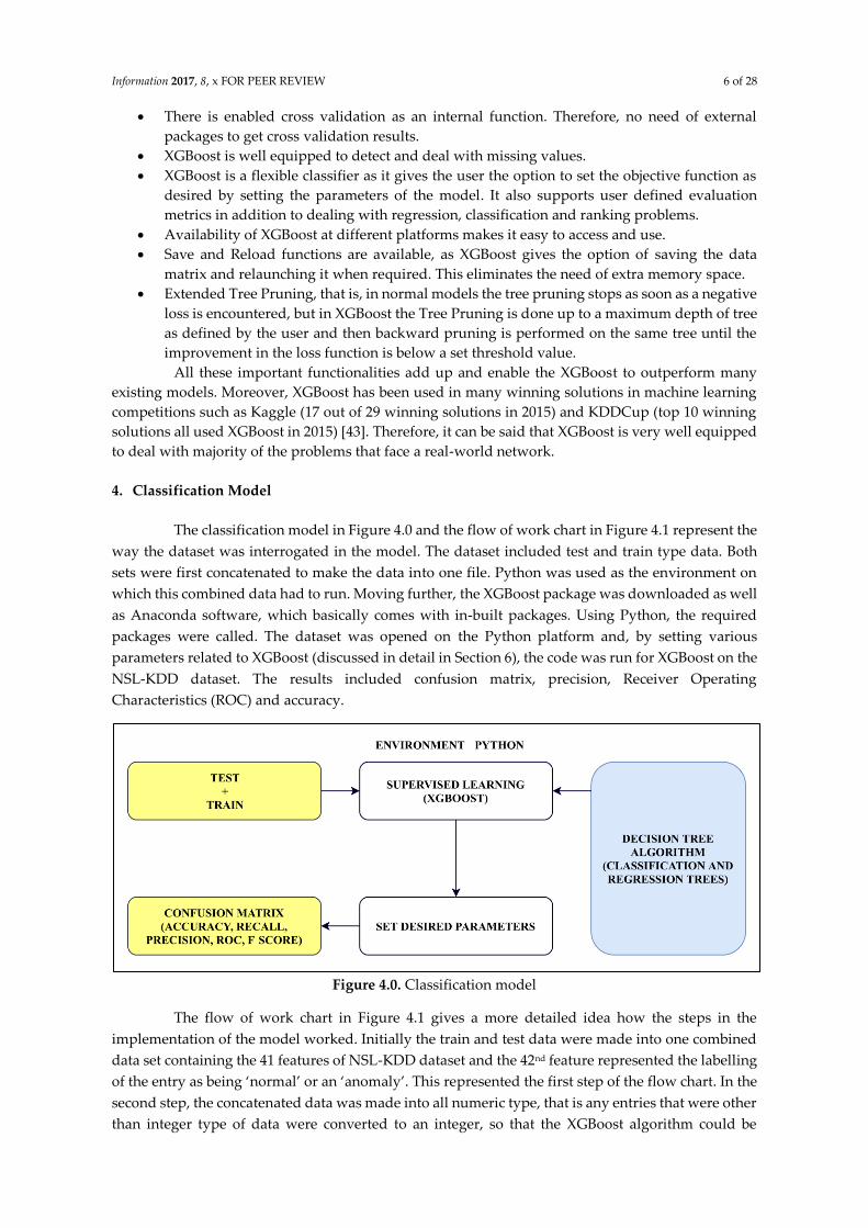
The classification model in Figure 4.0 and the flow of work chart in Figure 4.1 represent the

way the dataset was interrogated in the model. The dataset included test and train type data. Both

sets were first concatenated to make the data into one file. Python was used as the environment on

which this combined data had to run. Moving further, the XGBoost package was downloaded as well

as Anaconda software, which basically comes with in-built packages. Using Python, the required

packages were called. The dataset was opened on the Python platform and, by setting various

parameters related to XGBoost (discussed in detail in Section 6), the code was run for XGBoost on the

NSL-KDD dataset. The results included confusion matrix, precision, Receiver Operating

Characteristics (ROC) and accuracy.

Figure 4.0. Classification model

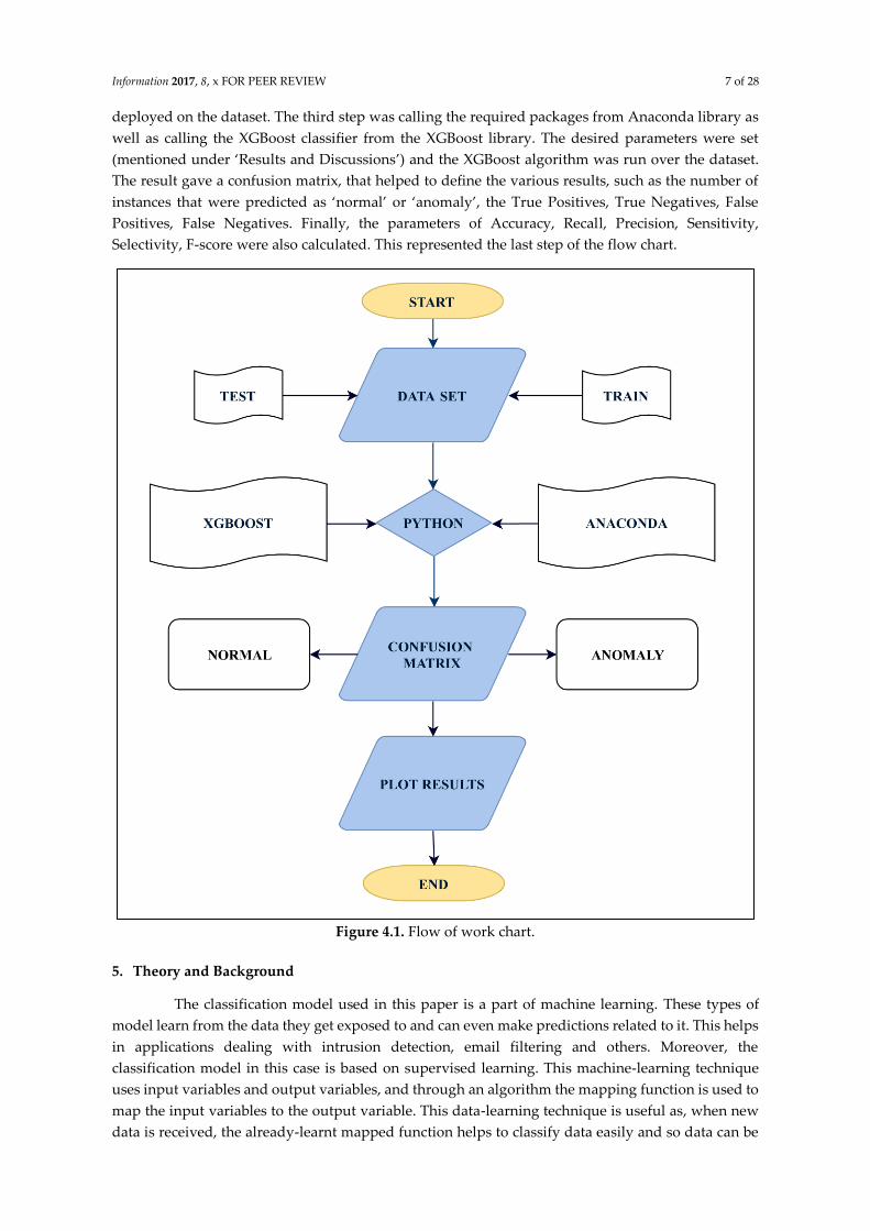
The flow of work chart in Figure 4.1 gives a more detailed idea how the steps in the

implementation of the model worked. Initially the train and test data were made into one combined

data set containing the 41 features of NSL-KDD dataset and the 42nd feature represented the labelling

of the entry as being ‘normal’ or an ‘anomaly’. This represented the first step of the flow chart. In the

second step, the concatenated data was made into all numeric type, that is any entries that were other

than integer type of data were converted to an integer, so that the XGBoost algorithm could be


deployed on the dataset. The third step was calling the required packages from Anaconda library as

well as calling the XGBoost classifier from the XGBoost library. The desired parameters were set

(mentioned under ‘Results and Discussions’) and the XGBoost algorithm was run over the dataset.

The result gave a confusion matrix, that helped to define the various results, such as the number of

instances that were predicted as ‘normal’ or ‘anomaly’, the True Positives, True Negatives, False

Positives, False Negatives. Finally, the parameters of Accuracy, Recall, Precision, Sensitivity,

Selectivity, F-score were also calculated. This represented the last step of the flow chart.

Figure 4.1. Flow of work chart.

5. Theory and Background

The classification model used in this paper is a part of machine learning. These types of

model learn from the data they get exposed to and can even make predictions related to it. This helps

in applications dealing with intrusion detection, email filtering and others. Moreover, the

classification model in this case is based on supervised learning. This machine-learning technique

uses input variables and output variables, and through an algorithm the mapping function is used to

map the input variables to the output variable. This data-learning technique is useful as, when new

data is received, the already-learnt mapped function helps to classify data easily and so data can be


separated or filtered. Hence, data are used to learn and build an algorithm and, based on the learned

algorithm, data is predicted; this very concept makes the core of any machine-learning classification

model. There are three main concepts around which the whole results revolve. They are Decision

Trees, Boosting and XGBoost. Each will be looked at to give a general view of the main ideas they

include.

5.1. Boosting

Boosting, a machine-learning algorithm, can be used to reduce bias and variance from the

dataset. Boosting helps to convert weak learners to strong ones. A weak-learner classifier is weakly

correlated with the true classification, whereas strong learners are strongly correlated. Algorithms

that can do the above simply became known as “boosting”. Most algorithms iteratively learn weak

classifiers and add them to a strong one. The data added are weighted, so that data that are correctly

classified shed weight and those misclassified gain weight. All in all, the data gets reweighted when

building up a strong learner from a set of weak learners. Algorithms such as AdaBoost, an adaptive

boosting algorithm developed by Schapire and Freund (they won the Godel Prize for it) [24] are

recommended. The main variation between various boosting algorithms is the method of weighting

the training data and its hypothesis. In Python, XGBoost can be used. It is in an open-source library

which provides a boosting algorithm in Python and other languages such as C++ and Java.

5.2. Decision Trees

Decision trees are algorithms that classify instances based on feature values. Each node of

a decision tree is a feature in an instance that is waiting to be classified. A feature is picked up to split

the training data and it becomes the root node. A similar procedure is followed, and the tree starts

digging deep, making sub-trees until the same class subsets are formed. One of the limitations of

decision trees is diagonal portioning. However, Zhang [23] suggested ways to construct multivariate

trees by using new features with operators such as conjunction, negation and disjunction.

C4.5 - The most well-known algorithm to design decision trees is C4.5 (Quinlan, 1993). It

uses the Information Gain as the criterion to choose which feature can be made the splitting feature.

It accepts both numeric and symbolic values and generates a classification tree. It recursively splits

to form subsets of the same class. Its only limitation is, that it is allergic to diagonal partitioning and

works poorly when the density of points in some regions is low. However, multivariate trees have

been developed lately to solve the above problem (Brodley and Utgoff [25]).

RF – A random-forest classifier (Breiman, 2001) is made up of many classification trees. The

kth classification tree is a classifier denoted by an unlabelled input vector and a randomly generated

vector by selection of random features of the training data for each node. The randomly generated

vector of different classification trees in the forest are not related to each other but are generated by

the same distribution algorithm. For unlabelled data, each tree will provide a prediction or vote and

so, labelling is done. There are many more algorithms that can be used such as the J48 technique and

others.

5.3. XGBoost

XGBoost was mainly designed for speed and performance using gradient-boosted decision

trees. It represents a way for machine boosting, or in other words applying boosting to machines,

initially done by Tianqi Chen [26] and further taken up by many developers. It is a tool that belongs

to the Distributed Machine Learning Community (DMLC). XGBoost or eXtreme Gradient Boosting

helps in exploiting every bit of memory and hardware resources for tree boosting algorithms. It gives

the benefit of algorithm enhancement, tuning the model, and can also be deployed in computing

environments. XGBoost can perform the three major gradient boosting techniques, that is Gradient

Boosting, Regularized Boosting and Stochastic Boosting. It also allows for the addition and tuning of

regularization parameters, making it stand out from other libraries. The algorithm is highly effective

in reducing the computing time and provides optimal use of memory resources. It is Sparse Aware,


or can take care of missing values, supports parallel structure in tree construction and has the unique

quality to perform boosting on added data already on the trained model (Continued Training) [27].

6. Mathematical Explanation

XGBoost functions around tree algorithms. The tree algorithms take into account the

attributes of the dataset; they can be called features or columns and then these very features act as

the conditional node or the internal node. Now, corresponding to the condition at the root node, the

tree splits up into branches or edges. The end of the branch that does not produce any further edges

is referred to as the leaf node, and generally splitting is done to reach a decision. The diagram in

Figure 6.0 is a representation of how a decision tree or classification tree works, based on an example

dataset, predicting whether a passenger survives or not.

Figure 6.0. The working of Decision Trees

XGBoost also applies decision-tree algorithms to a known dataset and then classifies the

data accordingly. The concept of XGBoost revolves around gradient-boosted trees using supervised

learning as the principal technique. Supervised learning basically refers to a technique in which the

input data, generally the training data 𝑝𝑖 having multiple features (as in this case), is used to predict

target values 𝑠𝑖 .

The mathematical algorithm (referred to as the model) makes predictions 𝑠𝑖 based on

trained data 𝑝𝑖 . For example, in a linear model, the prediction is based on a combination of weighted

input features such as �̂�𝑖 = ∑ 𝜃𝑗𝑗 𝑝𝑖𝑗 [28]. The parameters need to be learnt from the data. Usually, 𝜃 is

used to represent the parameters and, depending on the dataset, there can be numerous parameters.

The predict value 𝑠𝑖 helps to classify the problem at hand, whether it be regression, classification,

ranking, or others. The main motive is to find the appropriate parameters from the dataset used for

training purposes. An objective function is set up initially which describes the model performance. It

must be mentioned that each model can differ depending on which parameter is used. Suppose that

there is a dataset in which ‘length’ and ‘height’ are features of the dataset. Therefore, on the same

dataset numerous models can be set up, depending on which parameters are used.


The objective function [28] comprises two parts: the first part is termed a training loss and

the second part is termed a regularization.

𝑜𝑏𝑗(𝜃) = 𝑇𝐿(𝜃) + 𝑅(𝜃) (1)

The regularization term is represented by R and TL is for Training Loss. The TL is just a

measure of how predictive the model is. Regularization helps to keep the model’s complexity within

desired limits, eliminating problems such as over-stacking or overfitting of data which can lead to a

less accurate model. XGBoost simply adds the prediction of all trees formed from the dataset, and

then optimizes the result.

Random Forest also follow the model of tree ensembles. Therefore, it can be said that the

boosted trees, in comparison to random forest, are not too much different in terms of their algorithmic

make-up, but they differ in the way we train them. A predictive service of tree ensembles should

work both for random and boosted trees. This is a major advantage of supervised learning. The main

motive is to learn about the trees, and the simple way to do it is to optimize the objective function

[28].

The question that arises here is how the trees are set up in terms of the parameters used. To

determine these parameters the structure of the trees and their respective leaf scores are to be

calculated (generally represented by a function 𝑓𝑡). It is not a straightforward task to train all the trees

in parallel. XGBoost tries to optimize the learned tree (training) and adds a tree at every step. One

question that arises is which tree to add at each step, the answer being to add the tree that fulfills the

objective of optimizing our objective function [28].

The new objective function (say at step t) takes the form of an expansion represented by

Taylor’s theorem, generally including up to the second order.

𝑜𝑏𝑗(𝑡) = ∑ [𝑚𝑖𝑓𝑡(𝑝𝑖) + 1

2 𝑐𝑖𝑓𝑡

2(𝑝𝑖)] + 𝑅(𝑓𝑡)𝑛𝑖=1 (2)

, where 𝑚𝑖 and 𝑐𝑖 are taken as inputs.

The result reflects the desired optimization for the new tree that wants to add itself to the

model. This is the way that XGBoost deals with loss functions such as logistic regression.

Moving further, regularization plays an important part in defining the complexity of the

tree R(f). The definition of tree f(p) can be refined as [28]

𝑓𝑡(𝑝) = 𝑤𝑞(𝑝), 𝑤 𝜖 𝑅𝐿 , 𝑞: 𝑅𝑑 → {1,2,3,4 … , 𝐿}. (3)

In the above equation 𝑤 represents a vector for leaf scores (same score for data points using

the same leaf) and function q assigns leaves to the corresponding data points. L is the number of

leaves. In XGBoost the complexity is [28]

𝑅(𝑓) = 𝛼𝐿 + 1

2 𝛽 ∑ 𝑤𝑗

2.𝐿𝑗=1 (4)

Therefore, the equation of regularization can be put in Theorem (1), to get the new

optimized objective function at step t, or the tth tree. The resultant model represents the new reformed

tree model and is a measure of how good the tree structure q(p) is.

The tree structure is established by calculating the regularization, leaf scores, and objective

function at each level, as it is not possible to simultaneously calculate all combinations of trees. The

gain is calculated at each level as a leaf is split into a left leaf and a right leaf, and the gain is calculated

at the current leaf with the regularization achieved at the possible additional leaves. If the gain falls

short of the additional regularization value, then that branch is abandoned (concept also called

pruning). This is how XGBoost runs deep into trees and classifies data, and hence accuracy and other

parameters are calculated.


7. Results and Discussion

7.1. Dataset Used

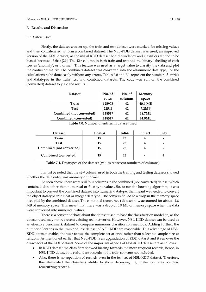
Firstly, the dataset was set up, the train and test dataset were checked for missing values

and then concatenated to form a combined dataset. The NSL-KDD dataset was used, an improved

version of the KDD dataset, as the initial KDD dataset had redundancy and classifiers tended to be

biased because of that [29]. The 42nd column in both train and test had the binary labelling of each

row as ‘anomaly’, or ‘normal’. This feature was used as a target value to classify the data and plot

the confusion matrix. The combined dataset was converted into the all-numeric data type, for the

calculations to be done easily without any errors. Tables 7.0 and 7.1 represent the number of entries

and datatypes in the train, test and combined datasets. The code was run on the combined

(converted) dataset to yield the results.

Dataset No. of

rows

No. of

columns

Memory

space

Train 125973 42 40.4 MB

Test 22544 42 7.2MB

Combined (not converted) 148517 42 48.7MB

Combined (converted) 148517 42 44.8MB

Table 7.0. Number of entries in dataset used

Dataset Float64 Int64 Object Int8

Train 15 23 4 -

Test 15 23 4 -

Combined (not converted) 15 23 4 -

Combined (converted) 15 23 - 4

Table 7.1. Datatypes of the dataset (values represent numbers of columns)

It must be noted that the 42nd column used in both the training and testing datasets showed

whether the data entry was anomaly or normal.

As seen above, there were still four columns in the combined (not converted) dataset which

contained data other than numerical or float type values. So, to run the boosting algorithm, it was

important to convert the combined dataset into numeric datatype; that meant we needed to convert

the object datatype into float or integer datatype. The conversion led to a drop in the memory space

occupied by the combined dataset. The combined (converted) dataset now accounted for about 44.8

MB of memory space. This meant that there was a drop of 3.9 MB of memory space when the data

were converted into numerical values.

There is a constant debate about the dataset used to base the classification model on, as the

dataset used may not represent existing real networks. However, NSL-KDD dataset can be used as

an effective benchmark dataset to compare numerous classification methods. Adding further, the

number of entries in the train and test dataset of NSL-KDD are reasonable. This advantage of NSL-

KDD dataset enables the user to use the complete set at once rather than selecting sample size at

random. As mentioned earlier that NSL-KDD is an upgradation of KDD dataset and it removes the

drawbacks of the KDD dataset. Some of the important aspects of NSL-KDD dataset are as follows:

• In KDD dataset the classifiers showed biasing towards the more frequent records, hence, in

NSL-KDD dataset the redundant records in the train set were not included.

• Also, there is no repetition of records even in the test set of NSL-KDD dataset. Therefore,

this eliminated the classifiers ability to show deceiving high detection rates courtesy

reoccurring records.


• As the number of records for each difficulty level group in NSL-KDD dataset is inversely

proportional to the percentage of records in the original KDD dataset, as a result the NSL-

KDD provided a wider range for the classification methods to do detection on. This made

NSL-KDD dataset more efficient in classification rates based on different classification

methods.

• One major reason to set the classification method on NSL-KDD dataset was to compare it

with the previously known results of different classification methods based on NSL-KDD

dataset (further elaborated in Table 7.6 under sub-section 7.6). This will make the evaluation

results more consistent and comparable.

7.2. Confusion Matrix

XGBoost has many parameters, and one can use these parameters to perform specific tasks.

The following are some of the parameters that were used to get the results (the purpose of the

parameters is also explained briefly) [30]:

• The ‘learning_rate’ (also referred to as ‘eta’) parameter is basically set to get rid of

overfitting problems. It performs the step size shrinkage, and weights relating to the new

features can be easily extracted (was set as 0.1).

• The ‘max_depth’ parameter is used to define how deep a tree runs: the bigger the value, the

more complex the model becomes (was set as 3).

• The ‘n_estimators’ parameter refers to the number of rounds or trees used in the model

(was set as 100).

• The ‘random_state’ parameter is also a learning parameter. It is also sometimes referred to

as ‘seed’ (was set as 7).

• The ‘n_splits’ parameter is used to split up the dataset into k parts (was set as 10).

The above-mentioned parameters are tree booster parameters and based on the above the

following results were calculated. There are many parameters that can be set up, but this mainly

depends on the user and the model. If parameters are not set, XGBoost picks up the default values,

though one can define the parameters as per the desired model.

The matrix in Figure 7.2 represents what a confusion matrix is made up of.

Figure 7.2. Confusion Matrix Representation


The quantities defined in Figure 7.2 will be used to calculate all the results achieved. There

are four main values, which are calculated by running the confusion matrix. These values are further

used to calculate the accuracy, precision, recall, F1 score, ROC curve and finally plot the confusion

matrix itself.

Elaborating, there are four main values: True Negative (TN) (negative in our dataset was

the target name ‘anomaly’ labelled as 0), True Positive (positive in our dataset was the target name

‘normal’ labelled as 1), False Negative and False Positive.

True Positive is a value assigned to an entry of the dataset when a known positive value is

predicted as positive, in other words if the color is red, and is predicted as red. True Negative is

when a known negative value is predicted as negative, that is the color is not red and is predicted as

being not red. On the other side, there is False Negative and False Positive. False Positive is when a

known positive value is predicted as negative, that is a known red color is predicted as not being

red. False Negative is the other way around, a known negative value is predicted as positive, that is

the red color is predicted when the known color was not red.

The Confusion Matrix represents the quality of the output of a classifier on any dataset. The

diagonal elements (blue box in Figures 7.2 and 7.2.1) represent correct or true labels, whereas the off-

diagonal (white box in Figure 7.2 and Figure 7.2.1) elements represent the elements misclassified by

the classification model. Therefore, the higher the values of the diagonal elements of the confusion

matrix, the better and more accurate the classification model becomes.

Figure 7.2.1 Confusion Matrix with Normalization

Figure Fig 7.2.1 represents the confusion matrix in normalized form, that is in numbers

between 0 and 1. It provides better and easier understanding of the data.

The different parameters of the Confusion Matrix represent the results giving TP, TN, FP

and FN. Using these, the specificity and sensitivity of the dataset can be calculated, which is just a

measure of how good the classification model is. The following were the results from the confusion

matrix:

• TP = 99.11% (0.991123108469).

• FP = 1.75% (0.0174775758085).

• FN = 0.89% (0.00887689153061).


• TN = 98.25% (0.982522424192).

FP and FN should be as low as possible, whereas TP and TN should be as high as possible.

The model is a good classification model as there is a high fraction of correct predictions as compared

to the misclassifications. Moreover, the sensitivity and specificity can be calculated.

• Sensitivity = TP/ (FN + TP) (also called TPR)

= 99.11%.

• Specificity = TN/ (TN + FP)

= 98.25%

• Therefore, FPR can be calculated:

FPR = (1 – specificity)

= (1- 0.9825)

= 0.0175

• As a cross-check, looking at Figure 7.2, TN + FN + FP + TP = N is the total number of

predictions. If we apply this formula, taking values from Figure 7.2.1, then the result comes

out to be N = (TN + FN + FP + TP) = (70214 + 684 + 1249 + 76370), the representation of values

in non-normalized form = 148517, that is the total number of entries (rows) in the combined

dataset. Therefore, the result obtained from the Confusion Matrix validates the dataset

entries.

The confusion matrix is the heartbeat of the classification model. Looking at the results

above, the classification model achieves very good results, but more parameters can be set up and

the best possible accuracy should be aimed at. The higher the values of TN and TP and the lower the

values of FN and FP, the stronger the model emerges. It must be mentioned here that this

classification model can form an integral part of an IDS in helping it to classify data as anomaly or

normal. The confusion matrix can be a source of data from which optimization of the model can be

initiated. By setting up more-specific parameters, accuracy, precision, recall and other results can be

optimized to achieve perfect results.

7.3. Accuracy/Recall/Precision

Figure 7.3 represents the plot of accuracy, precision and recall as fractions of K, K being the

value relating to the number of splits in tree formations.


Figure 7.3. Results for Accuracy, Precision and Recall

Initially, the combined dataset was run to generate the classification accuracy using only

two parameters, ‘test size’ = 0.33 and ‘seed’ = 7, then model generated an accuracy of 98.98%. This

reflected that the model was generating high accuracy with an error rate of a mere 1.02%. However,

when more parameters were set up as discussed earlier, the number of splits increased and as the

number of splits reached 8, the accuracy, precision and recall had a dip as seen above in Figure 7.3. It

could be seen that all these parameters were in direct relation to the number of splits. Explaining the

involved parameters, it can be said that the classification accuracy was basically dividing the number

of correct predictions by the total number of predictions made and multiplying the result by 100. The

accuracy calculated through XGBoost was:

Accuracy = (TP + TN) / (TP + FP + TN +FN) = 98.70%.

The Precision was calculated by dividing the number of True Positives (TP) by the total

number of True Positives and False Positives (FP) [31]. TP refers to the correct prediction of data being

normal (or positive), FP (also referred to as Type I error) refers to the incorrect prediction of data

being normal (or positive).

Precision = TP / (TP + FP) = 98.41%.

Moving further, the Recall parameter was calculated by dividing the number of TPs by the

total number of TPs and False Negatives (FNs). FN (Type II error) refers to the incorrect prediction

of data being an anomaly (or negative). There is something also called True Negatives (TN), which

refers to correct prediction of data being an anomaly (or negative).

Recall = TP / (TP + FN) = 99.11%.

The F1 score was also calculated; it is the average (weighted) of Precision and Recall. Even

though accuracy takes more limelight, it can be useful for an even class distribution (where FP and

FN are quite similar), but for an uneven class distribution where the cost of FP and FN are quite

different then it is more useful to look at the F1 score [32].


F1_Score =2*(Recall*Precision) / (Recall + Precision) =98.76%.

This is how XGBoost comes out with the results and, out of the three results, the best

results were for recall, followed by accuracy and precision. As the number of splits increases, there

is seen to be a decrease in the values because more splits allow the model to learn relations very

specific to a dataset.

7.4 ROC Curve

Figure 7.4 reflects how accurate the prediction is: the area under the curve is what reflects

the accuracy in prediction. A higher area under the curve is desired.

Figure 7.4. Receiver Operating Characteristic curve

The graph in Fig 7.4 is known as a ROC curve, and it represents the plotting of the True

Positive Rate (TPR) against the False Positive Rate (FPR). The TPR is also referred to as the

“sensitivity”, calculated the same way that Precision was calculated, that is (TP/(FN+TP)). The FPR on

the other hand is calculated as (1-specificity), where “specificity” is calculated as (TN/(TN+FP)). So, to

sum it up, the TPR is a measure of how often the prediction is correct, when there is a positive value,

and the FPR is how often the prediction is incorrect when the value is in fact negative. Looking at

Figure 7.4, it can be said that the closer is the curve to the left-hand and the top-hand borders of the

ROC plotting area, the more accurate the dataset. The area under the curve is a measure of accuracy

of the predictions; as seen above it is 0.99, which is excellent in terms of accuracy of the predictions.

ROC helps to achieve a trade-off between specificity and sensitivity [33].

7.5 Feature Score (F-Score)

Moving further, using an in-built function, the feature importance was also plotted. Figure

7.5.1 represents the result achieved.


Figure 7.5.1. Representation of F-Score

Table 7.5.2 * represents the meaning of the features used in the dataset [34].

Name of feature Meaning of feature

duration It represents the connection time.

protocol_type It represents the protocol used in the

connection.

service It represents the service used by the

destination network.

flag It represents the connection status (error or

no error).

dst_bytes The number of data bytes transferred from

destination to source in a single

connection.

src_bytes The number of data bytes transferred from

source to destination in a single

connection.

land It is 1 if source and destination IP

addresses and port numbers match, 0 if

not.

wrong_fragment It represents the number of wrong

fragments in a single connection.

urgent It represents the number of urgent packets

(urgent bit is present) in a single

connection.

hot It represents the number of root or

administrator indicators in the data sent,

that is whether the packet is entering the



system directory, and is it creating and

executing programs.

num_failed_logins It represents the number of times a login

attempt has failed.

logged_in It is 1 if successfully logged in, otherwise

0.

num_compromised It represents the number of compromised

positions in the data in a single connection.

root_shell It toggles to 1 if the root shell is obtained,

otherwise remains 0.

su_attempted It toggles to 1 if ‘su root’ command used,

otherwise remains 0.

num_root It represents the number of times

operations were performed as the root in

the connection.

num_file_creations It represents the number of times the file

creation command was used in the

connection.

num_shells It represents the number of shell prompts

encountered in the connection.

num_access_files It represents the number of times

operations were performed using access

control files.

num_outbound_commands It represents the number of times an

outbound command was issued in a

connection.

is_hot_login It represents whether the login belongs to

the root or administrator. If so 1, else 0.

is_guest_login It toggles to 1 if the login belongs to a

guest, otherwise remains 0.

count It counts the number of times the same

destination host is used as the current

connection in the past 2 seconds.

srv_count It represents the number of times a

connection in the past 2 seconds used the

same destination port number as that of

the current connection.

serror_rate The connections (in percentage) that used

‘flag’ s3, s2, s1 or s0 among the connections

aggregated in ‘count’.

srv_serror_rate The connections (in percentage) that used

‘flag’ s3, s2, s1 or s0 among the connections

aggregated in ‘srv_count’.

rerror_rate The connections (in percentage)

aggregated in ‘count’, that used the ‘REJ’

flag.

srv_rerror_rate The connections (in percentage)

aggregated in ‘srv_count’, that used the

‘REJ’ flag.



same_srv_rate The connections (in percentage)

aggregated in ‘count’, that used the same

service.

diff_srv_rate The connections (in percentage)

aggregated in ‘count’, that used a different

service.

srv_diff_host_rate The connections (in percentage)

aggregated in ‘srv_count’, that had a

dst_host_count

different destination addresses.

The feature counts when connections have

the same destination host IP address.

dst_host_srv_count The connections that used the same port

number.

dst_host_same_srv_rate The percentage of connections aggregated

in ‘dst_host_count’, that used the same

service.

dst_host_diff_srv_rate The percentage of connections aggregated

in ‘dst_host_count’, that used a different

service.

dst_host_same_src_port_rate The percentage of connections aggregated

in ‘dst_host_srv_count’, that used the same

port number.

dst_host_srv_diff_host_rate The percentage of connections aggregated

in ‘dst_host_srv_count’, that had a

different destination address.

dst_host_serror_rate The percentage of connections aggregated

in ‘dst_host_count’, that used ‘flag’ s3, s2,

s1 or s0.

dst_host_srv_serror_rate The percentage of connections aggregated

in ‘dst_host_srv_count’, that used ‘flag’ s3,

s2, s1 or s0.

dst_host_rerror_rate The percentage of connections aggregated

in ‘dst_host_count’, that used the ‘REJ’

flag.

dst_host_srv_rerror_rate The percentage of connections aggregated

in ‘dst_host_srv_count’, that used the ‘REJ’

flag.

Table 7.5.2. Meaning of Features used in the dataset

Figure 7.5.1 showed that the feature representing ‘dst_bytes’ was the most important

attribute as it had the highest F-score and on the other hand num_shells was the least important

attribute as it had the lowest F-score. It must be noted that the F-score was calculated by setting up

a model having parameters defined as:

• ‘learning_rate’ - 0.1, ‘max_depth’ - 5, ‘sub-sample’ - 0.9, ‘colsample_bytree’ - 0.8,

‘min_child_weight’ – 1, ‘seed’ – 0, and ‘objective’:’binary: logistic’ (Why are these specific

values chosen? look at Table 7.5.3 and Table 7.5.4).

The following are some of the additional parameters used and their meaning:

• The ‘min_child_weight’ parameter defines the required sum of instance

weight in a child. If the sum of instance weights in a leaf node falls short of

this parameter, further steps are abandoned.


• The ‘subsample’ parameter allows XGBoost to run on a limited set of data

and prevents overfitting.

• The ‘colsample_bytree’ parameter corresponds to the ratio of columns in

the subsample when building trees.

• The ‘objective’: ‘binary: logistic’ parameter is a learning parameter and is

used to specify the task undertaken: in this case uses logistic regression for

binary classification.

It must be mentioned that various combinations of parameters having different

values were run, and every time the attribute importance did not change for the most

important attribute, as ‘dst_bytes’ received the highest F-score each time the parameter

values were changed. However, the least important end changed with a change in

parameter values. So, it can be said that the parameters did have a direct effect on the F-

scores of the attributes, as any change in parameters reflected a change in the F-score of the

attributes in the NSL-KDD dataset. We set up the model parameters as above, as running

the code with these values had given the best results in terms of mean and standard

deviation. This will be elaborated further.

The following were some of the F-scores using the above-mentioned parameters:

• ‘dst_bytes’ - this attribute of the dataset accounted for the highest F-score of about 579.

• ‘num_shells’ and ‘urgent’ – this attribute of the combined test and train dataset accounted

for the least F-score of 1.

Further, more features were extracted out of the dataset importing GridSearchCV from the

sklearn package. This functionality of sklearn enabled us to evaluate the grid score, which showed

the mean and the corresponding standard deviation of the dataset using parameters such as

‘subsample’, ‘min_child_weight’, ‘learning_ rate’, ‘max_depth’, and others. The following were some

of the results:

• Two models were run. In the first model, the following were fixed parameters: ‘objective’:

‘binary: logistic’, ‘colsample_bytree’ – 0.8, ‘subsample’ – 0.8, ‘n_estimators’ – 1000, ‘seed’ –

0, ‘learning_rate ‘- 0.1. The model was run to calculate the best values of the mean and the

corresponding standard deviation for different combinations of the parameters

‘min_child_weight’ and ‘max_depth’. Table 7.5.3 represents the result achieved.

Parameters

‘max_depth’ ‘min_child_weight’ Mean Standard

Deviation

3 1 0.99913 0.00013

3 3 0.99907 0.00010

3 5 0.99894 0.00014

5 1 0.99921 0.00015

5 3 0.99914 0.00013

5 5 0.99907 0.00010

7 1 0.99919 0.00018

7 3 0.99913 0.00014

7 5 0.99905 0.00015

Table 7.5.3. Model 1

From the above it can be seen that the highest mean was 0.99921 achieved when the

‘min_child_weight’ and ‘max_depth’ parameters were set as 1 and 5 respectively, therefore

these parameter values were used while plotting the feature score (Figure 7.5.1).

• In the second model, the following parameters were fixed: ‘min_child_weight’ – 1, ‘seed’ –

0, ‘max_depth’ – 3, ‘n_estimators’ – 1000, ‘objective’: ‘binary: logistic’, ‘colsample_bytree’ –

0.8. The model was run to calculate the best values of mean and standard deviation for


different combinations of the parameters of ‘learning_rate’ and ‘subsample’. Table 7.5.4

represents the result achieved.

Parameters

‘learning_rate’ ‘subsample’ Mean Standard

Deviation

0.1 0.7 0.99912 0.00016

0.1 0.8 0.99913 0.00013

0.1 0.9 0.99917 0.00013

0.01 0.7 0.99601 0.00028

0.01 0.8 0.99589 0.00022

0.01 0.9 0.99583 0.00023

Table 7.5.4. Model 2

From the above it can be seen that the highest mean was 0.99917, achieved when the

‘learning_rate’ and ‘subsample’ parameters were set as 0.1 and 0.9 respectively.

The higher the value of the mean the better the accuracy of the model is, and hence the

better the readings will be reflected at the confusion matrix, ROC, precision and recall results.

Looking at models 1 and 2, the parameters were set up and the F-score was calculated as seen in

Figure 7.5.1. Therefore, now it can be understood why the parameters as discussed in the feature

score (Figure 7.5.1) were set up, as they accounted for higher mean values as seen in models 1 and 2,

though one can choose a new model by assigning parameter values as desired and based on those

very values the F-score can be calculated.

There can be many combinations to find the best parameter values used to set up a final

model. The whole motive is to find a model which gives the best results. The higher the mean values,

the better the model is to predict accuracy and other targets. The above two models were run to just

know the effect of parameters on a model. The best-fit values can be extracted and used in future

models so that accuracy reaches close to 100%. Every model has a different feature score; all it

depends on is the value of parameters set. Models 1 and 2 were run and extracting from these two

models the best-fit parameters, a final model was set up. The feature score was plotted in relation to

the final model as seen in Figure 7.5.1.

7.6 Comparison with other Classification Methods

The NSL-KDD dataset has been used as a dataset to test different classification methods by

many researchers. The Table 7.6 displays the various results achieved by various classification

models. The Accuracy of these methods has been displayed in Table 7.6 to establish why XGBoost

needs to be looked at as a strong classification model. Looking at the work of many researches as

referenced in Table 7.6, XGBoost brings about the best results out of the NSL-KDD dataset. The

accuracy achieved by XGBoost model of 98.70 % is the best as compared to the other models

employed on the same dataset. It must be mentioned that the same dataset was used to measure the

results and XGBoost sits at the top in terms of giving an accuracy in the classification of data. The

Random Forest technique which is widely used gave an accuracy of 96.12 % [38]. It must be

mentioned that these classification techniques in Table 7.6 are some of the major classification

techniques tested and based on them researchers even carry out hybrid models, in which two or

more techniques in one model are used. The results are promising in those, but it must be noted that

XGBoost implemented independently gave such promising results. Therefore, there is such a large

room of optimizing the results achieved by XGBoost by carrying out more researches, using hybrid

models as well which can be based on XGBoost. It can be easily said that XGBoost is a solid approach

and the results it generated cannot be overlooked as they present a huge room of improvement by


playing with the parameters of the desired model.

A brief description of the various classification methods used in Table 7.6 are as follows:

• Decision Table – In this classification model, an entry follows a hierarchical structure and the

entry at a higher level in the table gets split into a further table based on a pair of additional

attributes.

• Logistic – is a classification model which is a typical regression model in which the

relationship between various variables is analysed. The relationship between dependent and

independent variables is looked at.

• SGD – a classifier based on linear models with stochastic gradient descent learning. The

gradient related to the loss is estimated at each sample at a time.

• Random Forests and Random Trees – this classification method basically employs decision

trees to classify data.

• Stochastic Gradient Descent – a classification method also known as incremental gradient

descent. It is an iterative method deployed with the sole purpose of minimizing the objective

function.

• SVM – It is a supervised learning method of classification. The training samples are

categorized in two categories and new samples are split into these two categories depending

on their respective closeness to the respective two categories.

• Bayesian Network – In this classification method a directed acyclic graph or DAG is used.

The various nodes in the DAG represents the features and the arcs between the adjacent

nodes represent the dependencies. It is a method based on conditional probability.

• Neural Networks – A backpropagation algorithm is used implementing feedforward

network.

• Naïve Bayes – This classification method is based on probabilistic classifiers using Bayes

theorem.

• CART – decision trees employing Classification and Regression Trees.

• J48 – a decision tree classification method based on greedy algorithm.

• Spegasos – Implements the stochastic variant of the Pegasos (Primal Estimated sub-Gradient

solver for SVM).

The most important thing in an IDS is the environment it is set in. The type of data-entries

in the IDS are directly related to the type of environment the IDS is deployed in. This is where

XGBoost gets an advantage as it is flexible in its implementation. XGBoost can take many data-types

as the input entries and gives the choice of simultaneously running on different Operating Systems

such as Linux and Windows. Moreover, data overfitting problems are handled well in XGBoost and

the XGBoost offers the flexibility of applying the Decision Tree Algorithms as well as Linear Model

Solvers. The results in Table 7.6 are the appropriate comparisons between the different classification

methods.

Classifier Accuracy on NSL-KDD Dataset (%)

Proposed XGBoost 98.7

Decision Table [36] 97.5

Logistic [39] 97.269

SGD [39] 97.443

RBF Classifier [36] 96.7

Rotation Forest (using 5 classes for labelling

data as Normal and (Probe, DoS, R2L, and

U2R) as Anomaly) [38]

96.4

SMO (Sequential Minimal Optimization) [36] 96.2


Random Tree (using 5 classes for labelling



96.14

Random Forest (using 5 classes for labelling



96.12

Spegasos [36] 95.8

Stochastic Gradient Descent [36] 95.8

SVM [36] 92.9

Bayesian Network [36] 90.0

RBF Network [36] 87.9

Naïve Bayes [36] 86.2

CART (using 5 classes for labelling data as

Normal and (Probe, DoS, R2L, and U2R) as

Anomaly) [37]

81.5

ANN (Artificial Neural Network) (binary

class) [35]

81.2

J48 (using 5 classes for labelling data as

Normal and (Probe, DoS, R2L, and U2R) as

Anomaly) [37]

80.6

Voted Perception [36] 76.0

Self-Organizing Map (SOM) (Neural

Network) [36]

67.8

Table 7.6. Comparison among different classification methods.

There is always a constant comparison between different classification methods, and

researchers have always struggled to find the optimum classification method. Lately, researches

have contested the implementation of XGBoost and the RF classification method on datasets to find

the better classification model. The results do give XGBoost an advantage over the RF classification

method [40]. Moreover, XGBoost can parallelly do classification on multiple operating systems [41]

and by setting the parameters the desired decision tree algorithm can be run on XGBoost, that is

XGBoost can be the desired algorithm plus the boosting applied to it. Therefore, it stands out and

should be considered an important player in the field of classification.

XGBoost compared to traditional Boosted models increases the speed up to 10 times and

hence, the classification model becomes better as in a network model speed plays an important role

[41]. XGBoost is quite flexible as it does not depend on the type of data entering a network, it can

easily convert the entering data into numeric type and from there can classify data at good speed

and accuracy. The overfitting and other problems related to other classification methods are easily

dealt by XGBoost. The catch in the model is that the parameters set in the XGBoost model play an

important role in defining the way the classification model brings about the result. There can be

numerous models based on XGBoost, the depth and splits related parameters of Decision Trees or

the Algorithm intended to run on XGBoost can be set, each such setting will generate a new model

and new results. Therefore, the flexibility XGBoost offers is of a very high standard. There may be

questions related to the type of environment XGBoost can be used in, but when companies such as

Google have tested and adopted this model on ground, it clearly tells that XGBoost is a go to

classification model [42].

8. Conclusions

The prediction of data is excellent in this classification model (Accuracy = 98.70%) and

based on this future research could be set up which can help in initiating models designed to detect

intrusions. This research can help to design an IDS of the future, especially when security remains


such an issue. The findings are a reflection as to how effective and accurate XGBoost is when it comes

to predicting a dataset. The findings are very accurate, and the error rate is very low. These findings

can be further elaborated to design Intrusion Detection Systems which are robust and can be

employed in architectures of the future such as IoT, 5G and others.

A lot of work has been done in the field of classification models and their importance when

it comes to the classification of data. As discussed earlier, classification methods such as SVMs, RBF,

Neural Networks, Decision Trees and others have been tested to classify data. Even the hybrid

models have come up which employ more than one methods. Many researches have been carried

out and as compared to most of the classification methods XGBoost gives relatively higher results.

XGBoost is a relatively new concept as compared to others and its results are making it a model to

investigate. Random Forests and hybrid models do come close to the accuracy achieved by XGBoost

classification method when employed on NSL-KDD dataset, but in a real environment the type of

data in a network will be different and that brings to the main question as to which classification

method to adopt. Countering this question many investigators have majorly tried to compare the RF

techniques and the XGBoost technique on various datasets, and the results give XGBoost an edge

over the RF counterpart. The other important thing is that the RF are very prone to overfitting, and

to achieve a higher accuracy, RF needs to create high number of decision trees, and moreover the

data needs to be resampled again and again, with each sample requiring to train the new classifier.

The different classifiers generated try to overfit the data in a different way, and voting is needed to

average out those differences. The re-training aspect of RF is eliminated in XGBoost techniques,

which basically add a new classifier to the already trained ensemble. This may seem a small

difference between the two techniques but when they will be applied to an IDS, then they can affect

the performance and complexity of the IDS in a big way. The only difference is that the XGBoost

requires more care in setting up.

Moving further, there are a few more things that add weight to XGBoost as being a perfect

classification method as this algorithm provides accuracy, feasibility and efficiency. It automatically

can operate parallelly on Windows and Linux (has both linear model solver as well as tree learning

algorithms) and is up to 10 times faster than the traditional GBM (Generalized Boosted Models).

Xgboost offers flexibility as to what type of input it can take, also accepts sparse input for both tree

and linear booster. XGBoost also supports customized objective and evaluation functions. As a real-

life application example, XGBoost has been widely adopted in industries such as Google, Tencent,

Alibaba, and more, solving machine learning problems involving Terabytes of real life data.

The success and impact of the XGBoost algorithm is very well documented in numerous

machine learning and data mining competitions. As an example, the records from machine learning

competition site ‘Kaggle’, show that majority of winning solutions use XGBoost (17 winning solutions

out of 29 used XGBoost in 2015). In the KDDCup competition in 2015, XGBoost was used by every

winning team in the top 10. The winning solutions were solutions to problems such as malware

classification; store sales prediction; motion detection; web text classification; customer behaviour

prediction; high energy physics event classification; product categorization; ad click through rate

prediction; hazard risk prediction and many others. So, it can be well established that the datasets

used in these solutions differed and many problems such as False Alarms, classification of data, high-

level pre-processing were dealt with, but the only thing that remained constant was the use of

‘XGBoost’ as the preferred classification technique (especially when it came to the choice of learner).

Many E-Commerce companies have also adopted XGBoost as the classification method for various

purposes, as seen by a leading German fashion firm (ABOUT YOU) employing XGBoost to do return

prediction in a faster and robust way. The company was able to process up to 12 million rows in a

matter of minutes achieving a high accuracy in predicting whether a product will be returned or not.

These are a few examples and XGBoost’s capability to use cloud as a platform makes it a hit in

emerging markets. The new technologies are all based around the concept of cloudification and

virtualization, and this is where XGBoost has an advantage. As its flexibility, no specific platform

need, multiple accessible languages, availability, high quality results in less time, handling of sparse


entries, out of core capability and distributed structure make it a well-suited classification method

(consumes less resources on top of that).

The most important factor that emerges in classification problems is the scalability and this

is where XGBoost is best at. It is highly scalable algorithm. It runs approximately ten times faster than

existing methods on a single platform, and scales to millions and billions of examples as per the

memory settings. The scalability is achieved through the algorithmic optimizations and smart

innovations such as: a unique tree learning algorithm for handling sparse data; a weighted quantile

procedure to handle the instance weights in approximate tree learning; the use of parallel and

distributed computation leading to quick learning which makes the model exploration faster; and

one of the most important strengths of XGBoost is the ability to provide out of core computation

which allows the data scientists to process data including billions of examples on a cheap platform

such as desktop.

These advantages have made XGBoost a go to algorithm for Data Scientists, as it has already

shown tremendous results in tackling large scale problems. It’s properties such as user defined

objective function make it highly flexible and versatile tool that can easily solve problems related to

classification, regression and ranking. Moreover, as an open source software, it is easily available and

accessible from different platforms and interfaces. This amazing portability of XGBoost allows

compatibility with major Operating Systems therefore breaking static properties of previously known

classification models. The new functionality that XGBoost offers is that it supports training on

distributed cloud platforms, such as AWS, GCE, Azure and others. This is a major advantage as the

new technologies related to IoT and 5G is all built around cloud, and XGBoost is also easily interfaced

with cloud dataflow systems such as Spark and Flink. XGBoost can be used through multiple

programming languages such as Python, R, C++, Julia, Java and Scala. XGBoost has already proven

to push the boundaries of computing power for boosted tree algorithm as it lays special attention to

model performance and computational speed. On a financial front XGBoost systems consume less

resources as compared to other classification models, they also help in saving and reloading of data

whenever required. The implementation of XGBoost offers advanced features for algorithm

enhancement, model tuning and computing environments. The assessment of all classification

methods leads to the choice of XGBoost being used as the classification method as it can solve real

world scale problems using less resources. The impact of XGBoost cannot be neglected and it can be

said that XGBoost employed as an integral part of IDS performing functions as described above can

emerge as a stronger classification model than many others.

The focus is to build a strong classification model for use in IDS. A strong classification

model means one which can give near-perfect results. This will lead to a stronger IDS, the IDS when

deployed in a certain network will make it more secure, and there will be much fewer chances of

intrusion as the classification model running is of very high standard. The next bit is using the IDS

as a sensor to alert the administrator about any irregularities. The IDS can be used as a one- stop

device to extract information about the network. So, IDS can also act as a data source and its machine

learning capabilities make it a flexible technology, avoiding regular updating. The IDS in future can

also be made interactive with IoT devices. It can also form an integral part of Artificial Intelligence,

as security is also a problem in the robotic world (even robots can be hacked). The airplanes, cars,

mobile networks, the world of IoT, Artificial Intelligence, smart devices, all need IDS sensors

employed in their architecture. Basically, anything that has internet and machines involved can use

IDS as a security feature.

The future world needs its privacy intact, so the developing robotic technology that will do

a lot of work in future needs IDS. There is nothing perfectly safe in a network and there must be an

IDS in a network to monitor everything, as people travelling in planes, cars, etc. should be able to

trust the machines that are responsible for dropping them home. For example, any hacking resulting

in a plane getting hijacked due to intrusions in the network can lead to devastating results.

Summarizing, why XGBoost needs to be a go to classification method because it offers

flexibility, and can simultaneously work on different operating systems, gives a higher accuracy, can

accept diverse data as inputs, offers both linear model solver and tree algorithms, and finally has


been deployed in industries to tackle Terabytes of data. Therefore, it is already accepted in society,

and is giving tremendous results.

Conflicts of Interest

“The authors declare no conflict of interest."

Acknowledgements

The work in this paper was supported by School of Engineering, Macquarie University,

Sydney, Australia.

References

1. Leswing, K. (2017). The massive cyberattack that crippled the internet. [online] Business Insider Australia.

Available at: https://www.businessinsider.com.au/amazon-spotify-twitter-githuband-etsy-down-in-

apparent-dns-attack-2016-10?r=US&IR=T [Accessed 9 Sep. 2017].

2. En.wikipedia.org. (2017). Virtual machine escape. [online] Available at:

https://en.wikipedia.org/wiki/Virtual_machine_escape [Accessed 9 Sep. 2017].

3. Kuranda, S. (2017). The 20 Coolest Cloud Security Vendors Of The 2017 Cloud 100. [online] CRN. Available at:

https://www.crn.com/slide-shows/security/300083542/the-20-coolest-cloud-security-vendors-of-the-2017-

cloud-100.htm [Accessed 3 Apr. 2018].

4. Ether.gtisc.gatech.edu. (n.d.). Ether: Malware Analysis via Hardware Virtualization Extensions. [online]

Available at: http://ether.gtisc.gatech.edu/ [Accessed 21 Mar. 2018].

5. Cisco. (2010). Zone-Based Policy Firewall Design and Application Guide. [online] Cisco. Available at:

https://www.cisco.com/c/en/us/support/docs/security/ios-firewall/98628-zone-design-guide.html

[Accessed 21 Mar. 2018].

6. Mohammadreza Ektefa, Sara Memar, Fatimah Sidi, Lilly Suriani Affendey. Intrusion Detection using Data

Mining Techniques. In: International Conference on Information Retrieval and Knowledge Management;

2010. p. 200–204.

7. Holden, N. and Freitas, A. (2008). A Hybrid PSO/ACO Algorithm for Discovering Classification Rules in Data

Mining. [online] Available at: https://www.hindawi.com/journals/jaea/2008/316145/abs/ [Accessed 26 Mar.

2018].

8. Ardjani, F. and Sadouni, K. (2010). International Journal of Modern Education and Computer Science (IJMECS).

[online] Mecs-press.org. Available at: http://www.mecs-press.org/ijmecs/ijmecs-v2-n2/v2n2-5.html


9. Panda, M. Abraham, A. and Patra, M.R. (2011). A Hybrid Intelligent Approach for Network Intrusion Detection

[online] Isda2002m.softcomputing.net. Available at: http://isda2002m.softcomputing.net/panda2011.pdf


10. Dennis Petrussenko (2009). Incrementally Learning Rules for Anomaly Detection [online] Cs.fit.edu. Available

at: http://cs.fit.edu/~pkc/theses/petrusenko09.pdf [Accessed 26 Mar. 2018].

11. Matthew V. Mahoney and Philip K. Chan (2003). Learning Rules for Anomaly Detection of Hostile Network

Traffic [online] pdfs.semanticscholar.org. Available at:

https://pdfs.semanticscholar.org/d171/56aff7fc07e0e5f649e16399bd456c3a1f6b.pdf [Accessed 26 Mar.

2018].

12. Matthew V. Mahoney and Philip K. Chan (2001). Packet Header Anomaly Detection for Identifying Hostile

Network Traffic [online] Cs.fit.edu. Available at: https://cs.fit.edu/~mmahoney/paper3.pdf [Accessed 26

Mar. 2018].

13. Gao Xiang, Wang Min. Applying semi-supervised cluster algorithm for anomaly detection. In: IEEE -

International Symposium on Information Processing, no. 3; 2010. p. 43–45

14. Qiang Wang and Vasileios Megalooikonomou (n.d.). A Clustering Algorithm for Intrusion Detection [online]

Citeseerx.ist.psu.edu. Available at:

http://citeseerx.ist.psu.edu/viewdoc/download?doi=10.1.1.59.4965&rep=rep1&type=pdf [Accessed 26 Mar.

2018].

15. Mao, C., Lee, H., Parikh, D., Chen, T. and Huang, S. (2009). Semi-supervised co-training and active learning-

based approach for multi-view intrusion detection. [online] Available at:

https://dl.acm.org/citation.cfm?id=1529735 [Accessed 26 Mar. 2018].


16. Chiu, C., Lee, Y., Chang, C., Luo, W. and Huang, H. (2010). Semi-supervised Learning for False Alarm

Reduction. [online] Available at: https://link.springer.com/chapter/10.1007%2F978-3-642-14400-4_46


17. M. Naga Surya Lakshmi and Radhika, Dr.Y. (2005). Effective Approach for Intrusion Detection using KSVM

and R [online] Jatit.org. (n.d.) Available at: http://www.jatit.org/volumes/Vol95No17/20Vol95No17.pdf


18. Monowar, H. B., Bhattacharyya, D. K. and Kalita, J. K. (2012). An Effective Unsupervised Network Anomaly

Detection Method [online] Cs.uccs.edu. Available at:

http://www.cs.uccs.edu/~jkalita/papers/2012/BhuyanMonowarICACCI2012.pdf [Accessed 26 Mar. 2018].

19. Terran Lane (n.d.). A Decision Theoretic, Semi-Supervised Model for Intrusion Detection [online]

pdfs.semanticscholar.org. Available at:

https://pdfs.semanticscholar.org/c8a7/904d518c0c33d1b86f7cccd037d0d1d1251f.pdf [Accessed 26 Mar.

2018].

20. Zhang Fu (2012). Multifaceted Defense Against Distributed Denial of Service Attacks: Prevention, Detection and

Mitigation [online] pdfs.semanticscholar.org. Available at:

https://pdfs.semanticscholar.org/eb7d/4c742f6cd110d9c96a08e398cc415c3a8518.pdf [Accessed 26 Mar.

2018].

21. Zhang Fu , Marina Papatriantafilou and Philippas Tsigas (2012). Mitigating Distributed Denial of Service

Attacks in Multiparty Applications in the Presence of Clock Drifts - IEEE Journals & Magazine. [online]

Ieeexplore.ieee.org. Available at: http://ieeexplore.ieee.org/abstract/document/6143953/ [Accessed 26 Mar.

2018].

22. Catania, C. and Garino, C. (2012). Automatic network intrusion detection: Current techniques and open issues.

[online] Available at: https://www.sciencedirect.com/science/article/pii/S0045790612001073?via%3Dihub


23. Fu, Z., Papatriantafilou, M. and Tsigas, P. (2011). CluB: A Cluster-Based framework for mitigating Distributed

Denial of Service attacks. [online] Available at: https://dl.acm.org/citation.cfm?id=1982297 [Accessed 3 Apr.

2018].

24. En.wikipedia.org. (n.d.). Boosting (machine learning). [online] Available at:

https://en.wikipedia.org/wiki/Boosting_(machine_learning) [Accessed 5 Nov. 2017].

25. Brodley, C. and Utgoff, P. (1995). Multivariate Decision Trees - Semantic Scholar. [online] Semanticscholar.org.

Available at: https://www.semanticscholar.org/paper/Multivariate-Decision-Trees-Brodley-

Utgoff/21a84fe894493e9cd805bf64f1dc342d4b5ce17a [Accessed 3 Apr. 2018].

26. Brownlee, J. (n.d.). A Gentle Introduction to XGBoost for Applied Machine Learning – Machine Learning Mastery.

[online] Machine Learning Mastery. Available at: http://machinelearningmastery.com/gentle-introduction-

xgboost-applied-machine-learning/ [Accessed 2 Mar. 2018].

27. Reinstein, I. (n.d.). XGBoost a Top Machine Learning Method on Kaggle, Explained. [online] Kdnuggets.com.

Available at: http://www.kdnuggets.com/2017/10/xgboost-top-machine-learning-method-kaggle-

explained.html [Accessed 2 Mar. 2018].

28. Xgboost.readthedocs.io. (n.d.). Introduction to Boosted Trees – xgboost 0.7 documentation. [online]

Available at: http://xgboost.readthedocs.io/en/latest/model.html [Accessed 3 Mar. 2018].

29. Unb.ca. (n.d.). NSL-KDD | Datasets | Research | Canadian Institute for Cybersecurity | UNB. [online] Available

at: http://www.unb.ca/cic/datasets/nsl.html [Accessed 16 Mar. 2018].

30. Xgboost.readthedocs.io. (n.d.). XGBoost Parameters — xgboost 0.7 documentation. [online] Available at:

http://xgboost.readthedocs.io/en/latest/parameter.html [Accessed 12 Mar. 2018].

31. Brownlee, J. (2014). Classification Accuracy is Not Enough: More Performance Measures You Can Use - Machine

Learning Mastery. [online] Machine Learning Mastery. Available at:

https://machinelearningmastery.com/classification-accuracy-is-not-enough-more-performance-measures-

you-can-use/ [Accessed 16 Mar. 2018].

32. Joshi, R. (2016). Accuracy, Precision, Recall & F1 Score: Interpretation of Performance Measures - Exsilio Blog.

[online] Exsilio Blog. Available at: http://blog.exsilio.com/all/accuracy-precision-recall-f1-score-

interpretation-of-performance-measures/ [Accessed 3 Apr. 2018].

33. Gim.unmc.edu. (n.d.). Plotting and Intrepretating an ROC Curve. [online] Available at:

http://gim.unmc.edu/dxtests/roc2.htm [Accessed 16 Mar. 2018].

34. pdfs.semanticscholar.org. (n.d.). [online] Available at:

https://pdfs.semanticscholar.org/1b34/80021c4ab0f632efa99e01a9b073903c5554.pdf [Accessed 26 Mar.

2018].

35. Yadav, A. and Ingre, B. (2015). Performance analysis of NSL-KDD dataset using ANN. [online]

www.researchgate.net. Available at:

http://ieeexplore.ieee.org/search/searchresult.jsp?searchWithin=%22Authors%22:.QT.Zhang%20Fu.QT.&newsearch=true

http://ieeexplore.ieee.org/search/searchresult.jsp?searchWithin=%22Authors%22:.QT.Marina%20Papatriantafilou.QT.&newsearch=true

http://ieeexplore.ieee.org/search/searchresult.jsp?searchWithin=%22Authors%22:.QT.Philippas%20Tsigas.QT.&newsearch=true


https://www.researchgate.net/publication/309698316_Performance_analysis_of_NSL-KDD_dataset_using_ANN [Accessed 10 May 2018].

36. Hussain, J. and Lalmuanawma, S. (2016). Feature Analysis, Evaluation and Comparisons of Classification

Algorithms Based on Noisy Intrusion Dataset. [online] www.sciencedirect.com. Available at:

https://www.sciencedirect.com/science/article/pii/S1877050916315927 [Accessed 10 May 2018].

37. Citeseerx.ist.psu.edu. (2013). A Detailed Analysis on NSL-KDD Dataset Using Various Machine Learning

Techniques for Intrusion Detection. [online] Available at:

http://citeseerx.ist.psu.edu/viewdoc/download;jsessionid=7C05CDF892E875A01EDF75C2970CBDB9?doi=

10.1.1.680.6760&rep=rep1&type=pdf [Accessed 10 May 2018].

38. Garg, T. and Singh Khurana, S. (2014). Comparison of classification techniques for intrusion detection dataset

using WEKA - IEEE Conference Publication. [online] Ieeexplore.ieee.org. Available at:

https://ieeexplore.ieee.org/document/6909184/ [Accessed 10 May 2018].

39. Chauhan, H., Kumar, V. and Pundir, S. (2013). A Comparative Study of Classification Techniques for Intrusion

Detection - IEEE Conference Publication. [online] Ieeexplore.ieee.org. Available at:

https://ieeexplore.ieee.org/xpls/icp.jsp?arnumber=6724320 [Accessed 10 May 2018].

40. Z., Z. (2016). What is better: gradient-boosted trees, or a random forest? - FastML. [online] Fastml.com. Available

at: http://fastml.com/what-is-better-gradient-boosted-trees-or-random-forest/ [Accessed 10 May 2018].

41. Cross Validated. (n.d.). Gradient Boosting Tree vs Random Forest. [online] Available at:

https://stats.stackexchange.com/questions/173390/gradient-boosting-tree-vs-random-forest [Accessed 10

May 2018].

42. Abzooba.com. (n.d.). Why XGBoost ? and Why is it so Powerful in Machine Learning – Abzooba. [online]

Available at: http://www.abzooba.com/blog/why-xgboost-and-why-is-it-so-powerful-in-machine-

learning/ [Accessed 10 May 2018].

43. Chen, T. and Guestrin, C. (2016). XGBoost: A Scalable Tree Boosting System. [online] Arxiv.org. Available at:

https://arxiv.org/pdf/1603.02754.pdf [Accessed 12 Jun. 2018].

Documents

Article Effective Intrusion Detection System using XGBoost · and others. XGBoost is employed on the NSL-KDD dataset to get the desired results. The whole motive is to learn about