Embed Size (px)
Citation preview

HAL Id: hal-03202986https://hal.archives-ouvertes.fr/hal-03202986
Submitted on 20 Apr 2021
HAL is a multi-disciplinary open accessarchive for the deposit and dissemination of sci-entific research documents, whether they are pub-lished or not. The documents may come fromteaching and research institutions in France orabroad, or from public or private research centers.
L’archive ouverte pluridisciplinaire HAL, estdestinée au dépôt et à la diffusion de documentsscientifiques de niveau recherche, publiés ou non,émanant des établissements d’enseignement et derecherche français ou étrangers, des laboratoirespublics ou privés.
Arresting-Cable System for Robust Terminal Landing ofReusable Rockets
Huan Zhang, Zhihua Zhao, Gexue Ren, Pengxiang Hu, Yunfei Yang,Zhongwen Pan, Francesco Sanfedino
To cite this version:Huan Zhang, Zhihua Zhao, Gexue Ren, Pengxiang Hu, Yunfei Yang, et al.. Arresting-Cable System forRobust Terminal Landing of Reusable Rockets. Journal of Spacecraft and Rockets, American Instituteof Aeronautics and Astronautics, 2021, 58 (2), pp.425-443. �10.2514/1.A34646�. �hal-03202986�

Arresting-Cable System for Robust Terminal Landingof Reusable Rockets
Huan Zhang,∗ Zhihua Zhao,† and Gexue Ren‡
Tsinghua University, 100084 Beijing, People’s Republic of China
Pengxiang Hu,§ Yunfei Yang,¶ and Zhongwen Pan**
China Academy of Launch Vehicle Technology, 100076 Beijing, People’s Republic of China
and
Francesco Sanfedino††
University of Toulouse, 31055 Toulouse, France
https://doi.org/10.2514/1.A34646
Recent successful recovery techniques for rockets require that rockets maintain a vertical configuration with zero
vertical and lateral velocities; otherwise, landings may fail. To relax this requirement, a new active-arresting system
(inspired by the arresting gears used on aircraft carriers) is proposed herein to achieve a robust landing, even if the
rocket deviates from the target position or has notable residual velocities and inclinations. The system consists of four
deployable onboard hooks above the rocket’s center of mass, an on-ground apparatus containing four arresting
cables forming a square capture frame, and four buffer devices to actively catch and passively decelerate the landing
rocket. To catch the rocket, the capture frame was controlled by servo motors via a simple proportional–derivative
controller. After catching, the buffer devices generate decelerating forces to stop its motion. A flexible multibody
model of the proposed system was built to evaluate its robust performance under various combinations of multiple
uncertainties, such as noise measurement, time delay in the motor, initial conditions, and wind excitation. Using a
quasi-Monte Carlomethod, hundreds of deviated landing caseswere generated and simulated. The results confirmed
the robustness of the proposed system for achieving successful terminal landings.
Nomenclature
A = area of the arresting cable, m2
ap = proportional gain
ch = damping coefficient of the spring damper, �N ⋅ s�∕mdh = width of a hook, mE = modulus of the arresting cable, GPaFf = sliding friction, N
H = height of the supporting truss frame, mhh = size of a hook, m
Jenginek= moment of inertia of the rocket’s engine relative to
OXYZ (k � xx, yy), kg ⋅m2
Jenginezz = polar moment of inertia of the rocket’s engine relativeto OXYZ, kg ⋅m2
kh = stiffness coefficient of the spring damper, N∕mLc = length from the center of mass to the top of the rocket
stage, mLh = length from the origin ofOXYZ to the top of the rocket
stage, mLr = length of the rocket stage, mlh = length of a hook, m
l0 = half-width of arresting area, ml1 = half-width of capture area, mmengine = mass of rocket’s engine, ton
mh = mass of a hook, kgmw = mass of a counterweight, tonRp = radius of the active pulley, m
Rr = radius of the rocket stage, mvpi
= reelout velocity of the active pulley i, m∕svwg = stationary wind speed, m∕sα = transfer rate of the pulley group, dimensionlessβ = the stiffness proportional to the Rayleigh damping
factorθ = angle between the arresting cable and the horizontal
line in the simplified theoretical model, radθh = initial deployment angle between a hook and the
rocket stage, radθw = wind angle, radλwg = ratio of root mean square of gust speed with respect to
stationary wind speed, %ρ = density of the arresting cable, kg∕m3
σr = root mean square of measurement noise, mτ = time delay of servo motor, s0 = differentiation with respect to dimensionless time
Subscripts
h = hookp = active pulleyr = rocket stagew = counterweight
I. Introduction
D EVELOPING reusable rockets is supposed to be a promisingtechnical path to reducing the cost of accessing and exploring
space [1–3]. To achieve this goal, more than a half-century ago,scientists and engineers began exploring different decelerating andlanding techniques to recover rockets or their parts [1–4]. One of themost successful attempts is the space shuttle program, which recov-ered its orbiter and the two solid boosters. However, the space
*Ph.D. Candidate, School of Aerospace Engineering; [email protected].†Associate Professor, School ofAerospaceEngineering; zhaozh@tsinghua.
edu.cn (Corresponding Author).‡Professor, School of Aerospace Engineering; [email protected].§Engineer, Beijing Institute of Space System Engineering; hupengxiang@
tsinghua.org.cn.¶Senior Engineer, Beijing Institute of Space System Engineering;
[email protected].**Senior Engineer, Beijing Institute of Space System Engineering;
[email protected].††Ph.D. Candidate, National Higher French Institute of Aeronautics and
Space; [email protected].

shuttle’s hard-landing technique demands testing and maintainingthe recovered parts, which increase rather than decrease launchingcosts [5]. Nevertheless, an exciting vertical-recovery technique hasrecently been demonstrated by both SpaceX and Blue Origin: twospace companies from the United States. By combining retropropul-sion engines and landing legs to realize a soft landing, both compa-nies have recovered and reused the first stages of their Falcon 9 [6]and New Shepard [7] rockets, respectively. These successes not onlyconvinced people that space can be accessed in a more economicallyfeasible way than before, but they also encouraged scientists fromother countries to develop their own techniques for reusable rockets.However, the precise and undamaged recovery of a rocket stageremains an extremely demanding task.There are mainly two steps toward recovering a rocket stage. The
first step is navigating the stage to a targeted landing place, and the nextstep is a soft terminal landing. In the first navigation step, significantachievements have been made by learning from various mature Marslanding technologies accumulated over the past 50 years [8,9]. Now,based on well-developed high-precision guidance technologies, theguidance errors have been diminished from kilometers to meters withnearly minimum fuel consumption [10–12]. In the second terminal-landing step, the current vertical-recovery technique requires not onlyadvanced engines that are capable of multiple restarts and thrustmodulation within a large range [13–15] but also an accurate controlsystem to prevent the rocket from crashing [16,17].Moreover, the highheat flux on the base plate [18] and the reconfigured aerodynamiccharacteristics [17] during the touchdown phase require thermal pro-tection for the structure and accurate landing [19].In practice, managing a rocket to achieve a safe terminal landing
with landing legs is a very tough task. First of all, landing a rocket is aone-shot process; and there are no second chances [16]. Second,when a rocket touches down, it must be kept vertical with nearly zerovertical or lateral velocities. At the same time, the engines must beshut down. If the rocket is leaning, if its speed is too high, or if itsengines are shut down too late, then the landing legs might fail withthe potential risk of explosion. It is estimated that the vertical landingspeed must be less than 2 m∕s and the inclination angle must be lessthan 5 deg to guarantee a successful landing [20,21]. According to avideo issued by SpaceX,‡‡more than five Falcon 9 rockets have failedto land under these narrow constraints. These expensive failures haveled us to think about developing an alternative landing approach thatsignificantly expands the margin for a safe recovery, reduces thestrain on the engines and control system, and achieves a higher rate ofsafe landings.Currently, the field of aeronautics already offers a provenmeans of
achieving a robust landing: the arresting gear used on aircraft carriersto recover airplanes within an incredibly short distance [22,23]. In atypical design, several arresting cables are strung across the deck ofthe carrier, and the pilot actively guides the plane to snag its tail hookon one of the cables. Then, the braking mechanism connected to thecable rapidly decelerates the airplane. This system is able to recoverairplanes of various weights and velocities. Moreover, the landingplanes are allowed to deviate from the orientation of the runwaycenterline; therefore, an airplane that is partially out of control maystill be rescued by an arresting-cable system.In this study, a novel terminal-landing technique is proposed to
recover reusable rockets. The basic concept is to turn the horizontalarresting-cable systems on aircraft carriers into a vertical configura-tion. Since there is no pilot in the rocket, the positions of the cables areactively adjusted to catch the rocket. The proposed arresting system ismounted on towers, which can be located on ground or ocean plat-forms. This system offers the following three features: 1) capturingrockets under deviations in their lateral landing positions, inclinationangles, lateral velocity, and angular velocity; 2) decelerating andstopping rockets with residual velocities within a prescribed maxi-mum distance, maximum acceleration, and maximum cable stress;and 3) maintaining the recovered rocket in a vertical and stableorientation after it has come to a stop.
The rest of this paper is organized as follows: Sec. II introduces theoverall design of the terminal-landing system; Sec. III establishes aflexible multibody dynamic model of the proposed system; Sec. IVprovides simulation results and statistical results to verify the accuracy,feasibility, and applicability of the proposed system; and Sec. V con-cludeswith the pros and cons of the proposed terminal-landing device.
II. Overall Design of the Terminal-Landing System
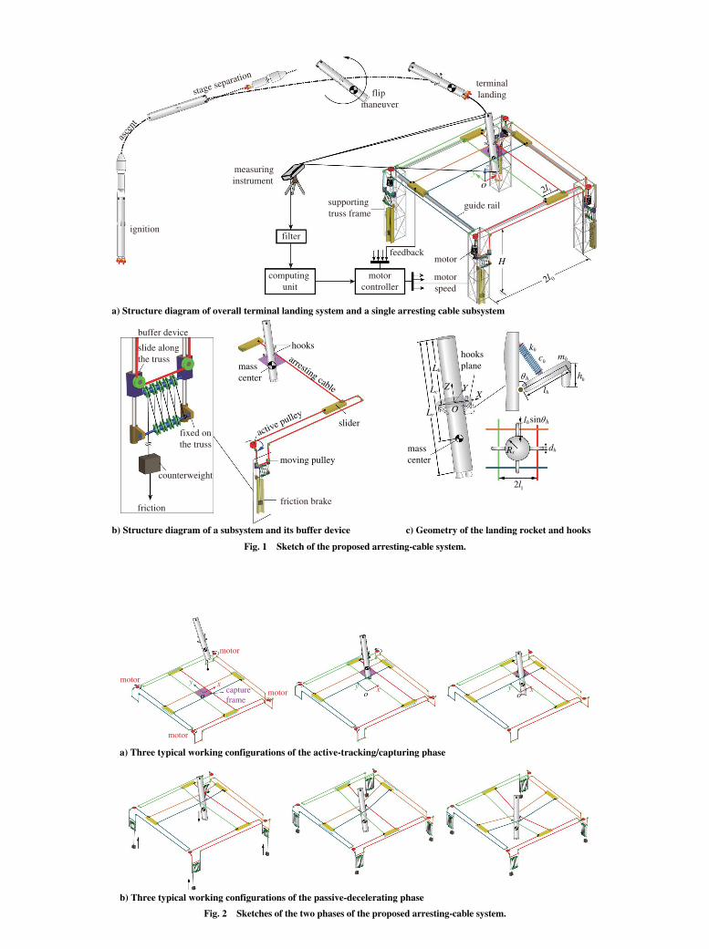
Figure 1a shows the overall structure of the proposed originalarresting-cable system for the recovery of a reusable rocket stage.The system has four supporting truss towers arranged in a square,four guide rails connecting these towers, and four sliders movingalong the rails. Along the rails are four identical arresting-cablesubsystems. As schematically shown in Fig. 1b, each subsystemhas a single cable connecting two opposing sliders after passingthrough several fixed passive pulleys, a fixed active pulley, andseveral moving pulleys. If the active fixed pulley is rotated, one slidercan be moved along the guide rail and dragged by one cable of asubsystem. The moving pulleys are connected to a buffer device thatconsists of a counterweight and a friction brake. The recoverablerocket itself is equipped with four hooks that are symmetricallydistributed above its center of mass.It is assumed the rocket stage is navigated to a target position, within
the supporting truss frame. With the process of the stage decent, thearresting cables are actively moved to catch the hooks. Once thesehooks are caught by the cables, the downwardmotion of the rocketwilldrag the buffer devices,which in turn generates decelerating forces thatslow the rocket. Because the hooks are located above the rocket’scenter ofmass, the resulting pendulummotion ensures that the rocket isstable. In summary, the four arresting-cable subsystems, together withthe hooks, are designed to track, capture, decelerate, and maintain thestability of the rocket during its landing phase.In this design, the entire landing process can be separated into two
sequential phases: 1) the active-tracking/capturing phase, and 2) thepassive-decelerating phase. During the first phase, as shown inFig. 2a, the counterweights are locked by friction, and the servomotors collectively reel in or reel out the cables to move the captureframe enclosed by the pre-tensioned arresting cables (as shown inpurple); this is done to catch the rocket. Catching occurs when therocket falls to a designated height and ends when the hooks engagewith the arresting cables. In the second phase, as shown in Fig. 2b, allmotors are powered down and the hooks drag the arresting cablesdownward, which in turn moves the counterweights upward andresults in frictional forces from the brakes. During this process, thekinematic energy of the rocket is partially transferred into gravita-tional energy of the counterweights and partially dissipated by thefriction of the brakes. Designing this landing device would requiretwo central tasks: creating a control algorithm for the motors in theactive-tracking/capturing phase, and designing the counterweightsand brakes of the buffer devices for the passive-deceleration phase.
A. Designing the Active-Tracking/Capturing Phase
Figure 3a shows the active-control system, which contains specifichardware (i.e., laser-measuring instruments, filters, a calculation unit,a controller, and four servo motors) and a proportional–differential(PD) algorithm for controlling themotors to actively track and capturethe landing rocket. This control systemaims to ensure that 1) the centerof the capture frame coincides with the target landing position of therocket, 2) the bottom of the rocket goes through the hollow captureframe, and 3) the hooks on the rocket catch the arresting cables.In designing the PD algorithm, the center position of the capture
frame is needed. However, obtaining that information is not a straight-forward task due to the fact that the frame is surrounded by flexiblecables. Fortunately, as shown in Fig. 3a, if the cables are sufficientlypre-tensioned, then the position of the capture frame could be approxi-mated by positions of the driven sliders. Therefore, the algorithmalternately controls the center positions of the sliders, which wereselected as control variables in the form of d � �xs1 ; xs2 ; ys3 ; ys4 �⊤.The effect of cable flexibility on the rocket capturing task is evaluatedin Sec. IV.
‡‡Data available online at https://www.youtube.com/watch?v=bvim4rsNHkQ [retrieved at 5 August 2019].
H
ignition
asce
nt
stage separationterminallandingflip
maneuver
buffer device
supporting truss frame
guide rail
fixed onthe truss
slide along the truss
counterweight
frictionfriction brake
hooks
mass center
active pulleyslider
a) Structure diagram of overall terminal landing system and a single arresting cable subsystem
b) Structure diagram of a subsystem and its buffer device c) Geometry of the landing rocket and hooks
arresting cable
moving pulleyRr
dh
sin hlh
hooksplane
Lr
Lh
Lc XZ
O
Y
mass center
lh
kh
h hh
mhhc
measuringinstrument
motor
motorcontroller
computing unit
filter
12l
motorspeed
feedback
xy z
02l
12lo
Fig. 1 Sketch of the proposed arresting-cable system.
capture frame
motor
motor
motor
motor
a) Three typical working configurations of the active-tracking/capturing phase
b) Three typical working configurations of the passive-decelerating phase
xy
oxy
oxy
o
Fig. 2 Sketches of the two phases of the proposed arresting-cable system.
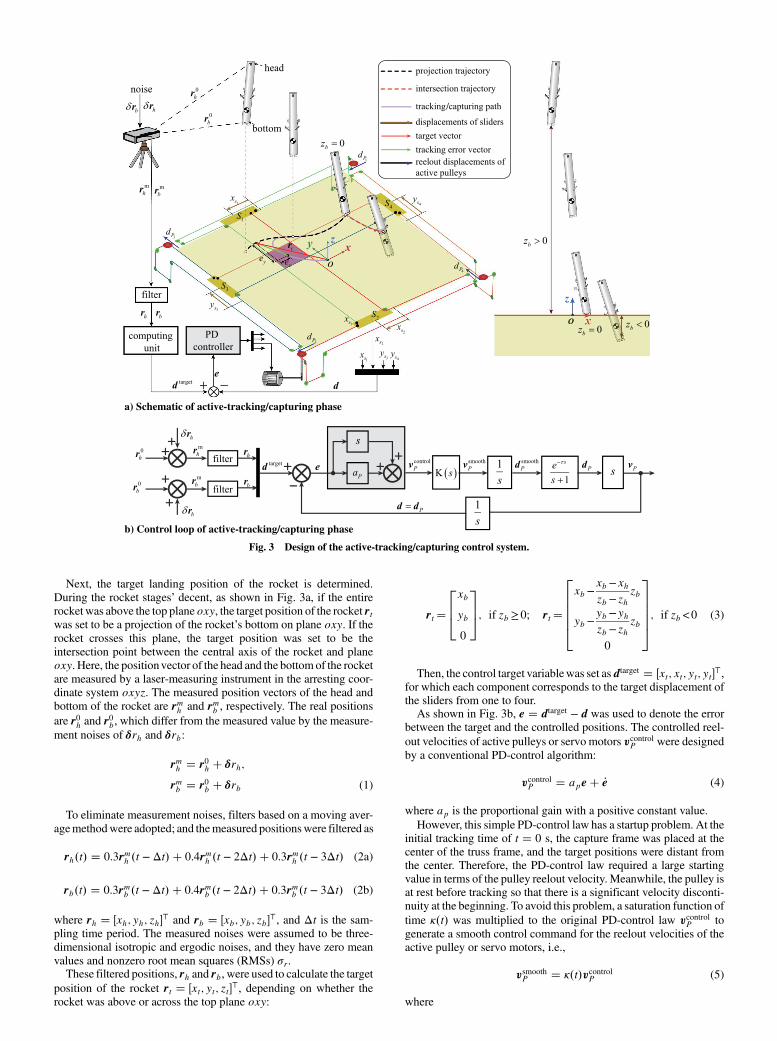
Next, the target landing position of the rocket is determined.
During the rocket stages’ decent, as shown in Fig. 3a, if the entire
rocket was above the top planeoxy, the target position of the rocket rtwas set to be a projection of the rocket’s bottom on plane oxy. If therocket crosses this plane, the target position was set to be the
intersection point between the central axis of the rocket and plane
oxy. Here, the positionvector of the head and the bottomof the rocket
are measured by a laser-measuring instrument in the arresting coor-
dinate system oxyz. The measured position vectors of the head and
bottom of the rocket are rmh and rmb , respectively. The real positionsare r0h and r
0b, which differ from the measured value by the measure-
ment noises of δrh and δrb:
rmh � r0h � δrh;
rmb � r0b � δrb (1)
To eliminate measurement noises, filters based on a moving aver-
agemethodwere adopted; and themeasured positionswere filtered as
rh�t� � 0.3rmh �t − Δt� � 0.4rmh �t − 2Δt� � 0.3rmh �t − 3Δt� (2a)
rb�t� � 0.3rmb �t − Δt� � 0.4rmb �t − 2Δt� � 0.3rmb �t − 3Δt� (2b)
where rh � �xh; yh; zh�⊤ and rb � �xb; yb; zb�⊤, and Δt is the sam-
pling time period. The measured noises were assumed to be three-
dimensional isotropic and ergodic noises, and they have zero mean
values and nonzero root mean squares (RMSs) σr.These filtered positions, rh and rb, were used to calculate the target
position of the rocket rt � �xt; yt; zt�⊤, depending on whether the
rocket was above or across the top plane oxy:
rt�
264xb
yb
0
375; if zb≥0; rt�
266664xb−
xb−xhzb−zh
zb
yb−yb−yhzb−zh
zb
0
377775; if zb <0 (3)
Then, the control target variablewas set as dtarget � �xt; xt; yt; yt�⊤,for which each component corresponds to the target displacement ofthe sliders from one to four.As shown in Fig. 3b, e � dtarget − d was used to denote the error
between the target and the controlled positions. The controlled reel-
out velocities of active pulleys or servo motors vcontrolP were designed
by a conventional PD-control algorithm:
vcontrolP � ape� _e (4)
where ap is the proportional gain with a positive constant value.
However, this simple PD-control law has a startup problem. At theinitial tracking time of t � 0 s, the capture frame was placed at thecenter of the truss frame, and the target positions were distant fromthe center. Therefore, the PD-control law required a large startingvalue in terms of the pulley reelout velocity. Meanwhile, the pulley isat rest before tracking so that there is a significant velocity disconti-nuity at the beginning. To avoid this problem, a saturation function of
time κ�t� was multiplied to the original PD-control law vcontrolP to
generate a smooth control command for the reelout velocities of theactive pulley or servo motors, i.e.,
vsmoothP � κ�t�vcontrolP (5)
where
a) Schematic of active-tracking/capturing phase
b) Control loop of active-tracking/capturing phase
Fig. 3 Design of the active-tracking/capturing control system.
κ�t� ��2t∕tc t < tc∕21 t ≥ tc∕2
(6)
and tc is the time duration of the active-tracking/capturing phase.Continuously inputting the control command vsmooth
P into the servo
motors, themotors’ time-delay feature makes the real output velocity
vP�t� and displacement dP�t� differ from the inputted target, assum-ing they satisfy the following discrete time-delay relationship [24]:
vP�t� � −dP�t� �Z
t−τ
0
vsmoothP �t̂� dt̂ (7)
where τ is the time-delay parameter. Additionally, the pre-tensioned
cables were wound tightly on the pulleys and are reeled in or out by
the motor; therefore, the reelout displacement of the active pulleyswas the same as the displacement of the sliders, namely, dP � d.Each of the four servo motors has an angular-displacement sensor
mounted on its shaft, enabling it to obtain the positions of the foursliders as well as the reelout displacement of the active pulleys. Thus,
the active-control system can be regarded as a closed control loop, as
shown in Fig. 3b.The transfer functionG�s� from the error vector e to the real reelout
velocities of the active pulleyvP can be obtained by doing theLaplacetransform to Eqs. (4–7), which can be expressed as follows:
G�s� ≜ VP�s�E�s� � �ap � s�e−τsK�s�
s� 1(8)
where s is the Laplace variable; and VP�s�, E�s�, and K�s� are theLaplace transforms of vp�t�, e�t�, and κ�t�. Based on this equation,
the effectiveness of the aforementioned designed control algorithm
on tracking the landing rocket was evaluated. The evaluation wasseparated into two steps: τ � 0 and τ ≠ 0.
First, assuming τ � 0, then the theoretical solution of the active-
control system for t < tc∕2 is as follows:
d � dtarget�1 − e−�ap∕tc�t2� (9)
Hence, the relative error is
���� e
dtarget
���� � e−�ap∕tc�t2 (10)
This response asymptotically converges to zero as long as ap is
positive. The larger the proportional gain of ap, the quicker the
converged result will be obtained. To obtain a fast convergence, such
as letting the relative error be less than e−5 at t � tc∕2, Eq. (10) saysthat the gain ap can be selected as
ap ≥ 20∕tc (11)
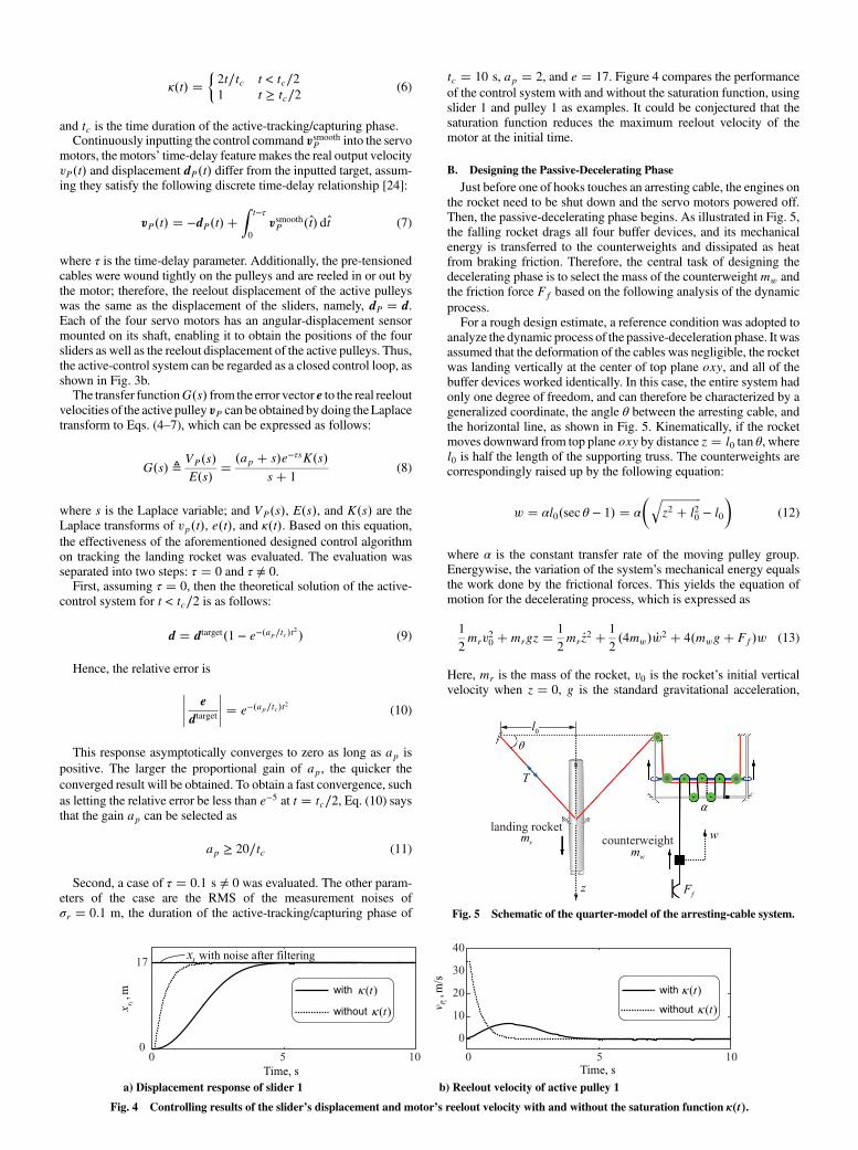
Second, a case of τ � 0.1 s ≠ 0 was evaluated. The other param-
eters of the case are the RMS of the measurement noises of
σr � 0.1 m, the duration of the active-tracking/capturing phase of
tc � 10 s, ap � 2, and e � 17. Figure 4 compares the performance
of the control system with and without the saturation function, usingslider 1 and pulley 1 as examples. It could be conjectured that thesaturation function reduces the maximum reelout velocity of themotor at the initial time.
B. Designing the Passive-Decelerating Phase
Just before one of hooks touches an arresting cable, the engines onthe rocket need to be shut down and the servo motors powered off.Then, the passive-decelerating phase begins. As illustrated in Fig. 5,the falling rocket drags all four buffer devices, and its mechanicalenergy is transferred to the counterweights and dissipated as heatfrom braking friction. Therefore, the central task of designing thedecelerating phase is to select the mass of the counterweightmw andthe friction force Ff based on the following analysis of the dynamic
process.For a rough design estimate, a reference condition was adopted to
analyze the dynamic process of the passive-deceleration phase. It wasassumed that the deformation of the cables was negligible, the rocketwas landing vertically at the center of top plane oxy, and all of thebuffer devices worked identically. In this case, the entire system hadonly one degree of freedom, and can therefore be characterized by ageneralized coordinate, the angle θ between the arresting cable, andthe horizontal line, as shown in Fig. 5. Kinematically, if the rocketmoves downward from top plane oxy by distance z � l0 tan θ, wherel0 is half the length of the supporting truss. The counterweights arecorrespondingly raised up by the following equation:
w � αl0�sec θ − 1� � α
� ���������������z2 � l20
q− l0
�(12)
where α is the constant transfer rate of the moving pulley group.Energywise, the variation of the system’s mechanical energy equalsthe work done by the frictional forces. This yields the equation ofmotion for the decelerating process, which is expressed as
1
2mrv
20 �mrgz �
1
2mr _z
2 � 1
2�4mw� _w2 � 4�mwg� Ff�w (13)
Here, mr is the mass of the rocket, v0 is the rocket’s initial verticalvelocity when z � 0, g is the standard gravitational acceleration,
a) Displacement response of slider 1 b) Reelout velocity of active pulley 1
Fig. 4 Controlling results of the slider’s displacement and motor’s reelout velocity with and without the saturation function κ�t�.
Fig. 5 Schematic of the quarter-model of the arresting-cable system.

and a dot over a symbol represents a differentiation with respect totime t.To make the analysis clearer and more concise, all quantities were
nondimensionalized and denoted by a bar over the symbols. Here, the
reference values of lengthwere chosen as l0, of time as����������l0∕g
p, and of
mass asmr. Thus, quantities of velocity were normalized by�������gl0
p, of
acceleration by g, and of force bymrg. Then, the equation of motion[Eq. (13)] could be reformulated into another dimensionless form as
�v202� �z � �z 02
2� �mt
α2�w 02
2�
�Ft
α�w (14)
where the prime symbol indicates a differentiation with respect to
dimensionless time �t ≜ t∕����������l0∕g
p, and
�mt ≜ 4α2 �mw; �Ft ≜ 4α� �mw � �Ff� (15)
were introduced to simplify the expression. In addition,
�w � α�sec θ − 1�; �z � tan θ (16)
To obtain an explicit expression for the velocity of the rocket, thekinematic expressions of Eq. (16) were differentiated with respect tothe dimensionless time �t. Also, �u 0, �z 0, and θ 0 are related as
�w 0 � α sin θ �z 0; θ 0 � �z 0cos2θ (17)
Substituting Eqs. (16) and (17) into Eq. (14) directly links thevelocity of the rocket with the generalized coordinate θ:
�z 02 � 2
1� �mtsin2θ
"�v202� tan θ − �Ft�sec θ − 1�
#(18)
Equation (18) implies that the dimensionless velocity is com-
pletely determined by two design parameters: namely, �mt and �Ft.Their selection fulfills the following three requirements:1) The rocket is stopped within an allowed dimensionless dis-
tance �zm.2) The maximum acceleration of the landing rocket is less than an
accepted dimensionless value �am.3) Themaximum tension in the cables is smaller than a dimension-
less tension �Tm to leave a sufficient margin for the cable strength.The proposed arresting system was designed for a rocket mass of
mass mr � 25 ton and a residual vertical velocity of v0 � 20 m∕s.Geometrically, the chosenhalf-length of the truss framewas l0 � 25 m,and the rocket was fully stopped when its displacement reached themaximum of zm � 10 m. For this system, the corresponding dimen-
sionless parameters are �v0 � v0∕�������gl0
p � 20∕��������������������9.81 × 25
p � 1.28and θm � arctan�10∕25� � 0.38 rad. Substituting the preceding
parameters and �z 0 � 0 into Eq. (18) yields a requirement on �Ft:
�Ft ��v20∕2� tan θmsec θm − 1
� 1.282∕2� tan 0.38
sec 0.38–1� 15.86 (19)
To obtain the acceleration value of the rocket, differentiatingEq. (18) with respect to the dimensionless time �t and making use ofthe relationships of Eqs. (17) and (19) yield the following:
�z 0 0 � 1 − �Ft sin θ
1� �mtsin2θ
−�mt sin�2θ�cos2θ�1� �mtsin
2θ�2��v202� tan θ − �Ft�sec θ − 1�
�(20)
Since both �v0 and �Ft are given, the maximum acceleration ofthe rocket only depends on the parameter �mt. Figure 6 gives thej�z 0 0jmax– �mt curve as a red solid line; it is not a monotonic function.Setting �am � 4 and then demanding j�z 0 0jmax ≤ �am require
�mt ≥ 1.55 (21)
To obtain the tension in the arresting cables, Newton’s second law
was applied to the rocket’s vertical direction, yielding
mr �z � mrg − 8T sin θ (22)
This equation can be nondimensionalized as
�T � 1
8 sin θ�1 − �z 0 0� (23)
Aswith the dimensionless acceleration of the rocket, themaximum
cable tension only depends on the parameter �mt. Figure 6 shows the�Tmax– �mt curve as a blue dashed line.
Fig. 6 The relationship between j �z 0 0jmax, �Tmax, and �mt.
Table 1 Physical parameters ofthe proposed terminal-landing system
Item Value
Rocket stage
Rr 2.00 m
Lr 40.00 m
Lc 30.00 m
mengine 12.50 tons
Jenginezz 2.50 × 10⁴ kg ⋅m2
Jenginexx � Jengineyy 4.16 × 10³ kg ⋅m2
EA 2.63 × 10⁹ N
ρA 501.40 kg∕mEJ 5.24 × 10⁹ N∕m
Hook
mh 45.00 kg
lh 3.50 m
hh 1.00 m
θh π∕3 rad
dh 0.15 m
kh 1.50 × 10⁵ N∕mch 4.00 × 10⁵ �N ⋅ s�∕mLh 20.00 m
Arresting-cable system
H ≥ 30.00 m
2l0 50.00 m
2l1 7.00 m
EA 2.64 × 10⁸ N
ρA 9.80 kg∕mRp 0.10 m
mw 0.92 ton
Ff 3.13 × 10⁵ N
α 3

Here, the arresting cable is the same type as that is used in aircraftcarriers. Its radius was 20 mm, and the allowed stress was 800 MPasuch that �Tm � 800 × π × 202∕�25 × 103 × 9.81� � 4.1. Therefore,
requiring �Tmax ≤ �Tm requires
�mt ≤ 10.2 (24)
In fulfilling the requirements of Eqs. (21) and (24), �mt was set totwo since this design is concerned more with cable tension than theacceleration of the rocket. Then, the mass of the counterweight mw
and the frictional force Ff were determined by the transfer rate αaccording to Eq. (15).The design and structural parameters of the system are listed in
Table 1. The center ofmass of the landing rocket was generally belowthe geometric center, and a 12.5 ton landing rocket mounted by anengine of 12.5 ton at its bottom was selected as the object of thisstudy. For simplicity, the mass of the rocket’s thin-walled structurewas uniformly distributed along the axial direction.
III. Dynamical Simulation Model
Although the design process described in the previous sectionassumed the rocket to be descending vertically with zero lateralvelocity and along the center of the supporting truss, these assump-tions are not needed for the proposed system. In particular, when therocket deviates from these working conditions (i.e., it is off centerfrom the truss frame, it is tilted, or it is moving sideways), then itsdynamics are much too complex to be computed analytically. There-fore, a dynamical simulation model was built to evaluate the landingperformance of the proposed arresting-cable system under differentlanding conditions.
A. Governing Equations of the System
The model was based on a multibody approach, as shown in Fig. 7.The truss structure, guide rails, pulleys, and sliders are all simplified asmassless rigid bodies because they are not important to the dynamicprocess. For each buffer device, the counterweight was considered as apoint mass, and the brake was replaced by a stick-slip friction force.
To consider the elastic vibration and small deformation of the rocket,the rocketwasmodeledby lumped rigidbodies connectedbymassless-beam elements [25]. The rigid hooks were hinged to the rocket andwere also connected to the rocket by springs and dampers. Thearresting cables were meshed with variable-length cable elementsbased on an arbitrary Lagrangian–Euler (ALE) description, and thecontacts between the hooks and cables were accounted for with Hertzcontact forces [26,27]. The control of the active-tracking/capturing
phase was integrated into the dynamic equation of the system in theform of state space. The details are presented in the following sub-sections. In summary, the governing equations of the arresting-cablesystem and the landing rocket form a set of differential algebraicequations (DAEs) [28]:
8>>>>>><>>>>>>:
M�q� �q�Φ⊤q λ −Q�q; _q; t� � 0
Φ�q; _q; vP; t� � 0
e � e�q; t�_x � Ax� Be
vP � Cx�De
(25)
Here, q is the generalized coordinate vector of the system; M�q� isthe mass matrix of the system; Q�q; _q; t� is the generalized forcevector of the forces applied to the system;Φ�q; _q; vP; t� is the vectorof the kinematic and geometric constraints; Φq is the gradient of
Φ with respect to q; λ is the corresponding Lagrange multiplier;
fA;B;C;Dg are the state-space matrices of the controller; x is thestate variables; and e and vP are the control input and output of thecontroller, respectively. The whole systemmodel was built using ourlaboratory’s in-house multibody code, and the obtained DAEs werenumerically integrated through an index-3 backward differentiationformula.
B. Modeling the Arresting Cables
The main difficulty in modeling the proposed recovery system isovercoming the problem of efficiency in modeling flexible arrestingcables with a large displacement, as well as the moving points of
a) Model during active-tracking/capturing phase b) Model during passive-decelerating phase
Fig. 7 Simulation model of the active arresting-cable system.
contacts between the hooks and cables. The traditional finite element
modeling method, based on the Lagrange formulation, meshes
the cable as a fixed grid of constant-length elements and calculates
the contact force between these cable elements and the hooks.
For contact detections, this method demands that the size of the
cable elements that are potentially contacting with the hooks is much
smaller than the hooks’ radius. Therefore, very fine elements are
necessary to mesh the cables if a large portion of them might make
contact. This fact significantly increases the calculation scale and
time.To substantially improve the calculation efficiency, a new model-
ing method was established to handle the cables and their contact
with the hooks. As shown in Fig. 7a, the basic idea was to dynami-
cally adjust the cable meshes to guarantee that only a few elements
contact the hooks and that these cable elements be finely meshed
while the others are roughlymeshed. Thus, the number of elements is
notably reduced and the contact detections are focused on a limited
range, thus accelerating the calculation. Technically speaking, this
meshing was implemented by combining a kind of variable-length
cable element and a length-adjusting algorithm.
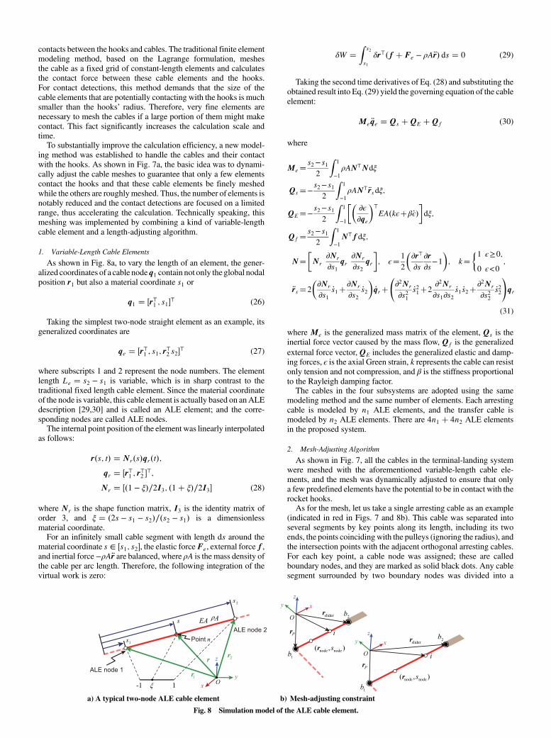
1. Variable-Length Cable Elements
As shown in Fig. 8a, to vary the length of an element, the gener-
alized coordinates of a cable nodeq1 contain not only the global nodalposition r1 but also a material coordinate s1 or
q1 � �r⊤1 ; s1�⊤ (26)
Taking the simplest two-node straight element as an example, its
generalized coordinates are
qe � �r⊤1 ; s1; r⊤2 s2�⊤ (27)
where subscripts 1 and 2 represent the node numbers. The element
length Le � s2 − s1 is variable, which is in sharp contrast to the
traditional fixed length cable element. Since the material coordinate
of the node is variable, this cable element is actually based on anALE
description [29,30] and is called an ALE element; and the corre-
sponding nodes are called ALE nodes.The internal point position of the element was linearly interpolated
as follows:
r�s; t� � Nr�s�qr�t�;qr � �r⊤1 ; r⊤2 �⊤;Nr � ��1 − ξ�∕2I3; �1� ξ�∕2I3� (28)
where Nr is the shape function matrix, I3 is the identity matrix of
order 3, and ξ � �2s − s1 − s2�∕�s2 − s1� is a dimensionless
material coordinate.For an infinitely small cable segment with length ds around the
material coordinate s ∈ �s1; s2�, the elastic forceFe, external force f ,and inertial force−ρA�r are balanced, where ρA is the mass density of
the cable per arc length. Therefore, the following integration of the
virtual work is zero:
δW �Z
s2
s1
δr⊤�f � Fe − ρA�r� ds � 0 (29)
Taking the second time derivatives of Eq. (28) and substituting the
obtained result into Eq. (29) yield the governing equation of the cable
element:
Me �qe � Qs �QE �Qf (30)
where
Me�s2−s1
2
Z1
−1ρAN⊤Ndξ
Qs�−s2−s1
2
Z1
−1ρAN⊤ �rsdξ;
QE�−s2−s1
2
Z1
−1
��∂ϵ∂qe
�⊤EA�kϵ�β_ϵ�
�dξ;
Qf�s2−s1
2
Z1
−1N⊤f dξ;
N��Nr
∂Nr
∂s1qr
∂Nr
∂s2qr
�; ϵ�1
2
�∂r⊤
∂s∂r∂s
−1
�; k�
�1 ϵ≥0;
0 ϵ<0;
�rs�2
�∂Nr
∂s1_s1�
∂Nr
∂s2_s2
�_qr�
∂2Nr
∂s21_s21�2
∂2Nr
∂s1∂s2_s1 _s2�
∂2Nr
∂s22_s22
!qr
(31)
where Me is the generalized mass matrix of the element, Qs is the
inertial force vector caused by the mass flow, Qf is the generalized
external force vector,QE includes the generalized elastic and damp-
ing forces, ϵ is the axial Green strain, k represents the cable can resistonly tension and not compression, and β is the stiffness proportionalto the Rayleigh damping factor.The cables in the four subsystems are adopted using the same
modeling method and the same number of elements. Each arresting
cable is modeled by n1 ALE elements, and the transfer cable is
modeled by n2 ALE elements. There are 4n1 � 4n2 ALE elements
in the proposed system.
2. Mesh-Adjusting Algorithm
As shown in Fig. 7, all the cables in the terminal-landing system
were meshed with the aforementioned variable-length cable ele-
ments, and the mesh was dynamically adjusted to ensure that only
a few predefined elements have the potential to be in contact with the
rocket hooks.As for the mesh, let us take a single arresting cable as an example
(indicated in red in Figs. 7 and 8b). This cable was separated into
several segments by key points along its length, including its two
ends, the points coinciding with the pulleys (ignoring the radius), and
the intersection points with the adjacent orthogonal arresting cables.
For each key point, a cable node was assigned; these are called
boundary nodes, and they are marked as solid black dots. Any cable
segment surrounded by two boundary nodes was divided into a
b) Mesh-adjusting constrainta) A typical two-node ALE cable element
Fig. 8 Simulation model of the ALE cable element.

number of elements by uniformly distributing internal nodes, marked
as hollow black dots.The positions of the mesh nodes were adjusted and determined by
introducing the following three kinds of constraint equations into the
model. First, if a boundary node is at the end of a cable, located on a
slider, then its position is the same as that of the slider and its material
coordinate is a constant since there is no material flow. The equation
is expressed as follows:
Φ1 �"rnode − rslider
snode − s0node
#� 0 (32)
where s0node is a constant for the material coordinate of the node at the
initial time.Second, if a boundary node coincides with a pulley or an inter-
section point, then its position rnode equals the corresponding pulley’sor point’s position rp; and the constraints relate only to position
[31,32] or are expressed as
Φ2 � rnode − rp � 0 (33)
Third, consider a cable segment bounded by two boundary nodes,
b1 and b2, whose material coordinates are sb1 and sb2 . The segment
was meshed into N elements by N − 1 internal nodes, and the
material coordinates of these internal nodes were distributed to
equally split the length of the segment. Then, the material coordinate
si of the ith node, numbered from the boundary node b1, wasdetermined to be
Φ3i � si − �sb1 � �sb2 − sb1�i∕N; � � 0 (34)
where i � 1; 2; : : : ; N − 1. The number N is set to be large for
the cable segments that contact the hooks and small for the other
segments [33].
C. Flexible Model of a Landing Rocket
Since the rocket’s propellant was nearly exhausted in the terminal-
landing phase, its structures were modeled as a flexible multibody
model in which a cluster of lumped rigid bodies was connected by
massless-beam elements [25] and the hooks and engines (as well as
the counterweights and sliders) were modeled by the rigid bodies and
constraints.
1. Rigid Bodies
As shown in Fig. 9, the generalized coordinates of a rigid body i inquaternion representation are
qi � �r⊤i ; θ⊤i �⊤ (35)
where ri are the position coordinates of the center of mass of the rigid
body i; and θi � �θ0i ; θ1i ; θ2i ; θ3i �⊤ are the orientation quaternion
parameters of the ith rigid body, which satisfies θ⊤i θi � 1.Taking the first time derivatives of Eq. (35), calculating the kinetic
energy of the ith rigid body Ti � 1∕2 _q⊤i Mi _qi, and substituting the
obtained result into the second kind of Lagrangian equation in
analytical mechanics yield the following governing equation of the
ith rigid body:
Mi �qi � Qq �Qf (36)
Here, Qq � − _Mi _qi � �∂Ti∕∂qi�⊤ is the generalized inertial force
vector, and Qf � Hif is the generalized external force vector.
In addition,
Mi �"miI3×3 0
0 4G⊤i JiGi
#; Hi �
"I3×3 03×4
04×3 2GTi
#(37)
Gi �
2664−θ1i θ0i θ3i −θ2i−θ2i −θ3i θ0i θ1i
−θ3i θ2i −θ1i θ0i
3775 (38)
where Ji is the inertial tensor of the ith rigid body.The external force vector f was determined by a combination of
gravity, the massless-beam force, aerodynamics, the spring-damper
force, the contact force, and the friction of different rigid bodies in
this system as follows:
f �
8>><>>:fgrav � fbeam � faero � f sprdmp �rocket�fgrav � fcontact � f aero � f sprdmp �hook�fgrav � f friction �counterweight�
(39)
This will be discussed in detail in the next subsection. The rocket
was clustered by nb rigid bodies and connected by nb − 1 massless-
beam elements. The four hooks, the four sliders, and the four counter-
weights were all modeled as rigid bodies and were constrained to
only one degree of freedom, as described in the following. Thus, there
are nb � 12 rigid bodies in this system.
2. Constraints of Rigid Bodies
In the arresting-cable system, the hooks on the rocket were
designed to only rotate relative the hinged pins, whereas the counter-
weights and sliders can only slide along the slideway and guide rails.
These constraints were modeled by a set of algebraic constraint
equations.For a revolute constraint between the rocket and a hook, revolution
was only allowed around the z axis of the two objects, as shown in theupper dotted box of Fig. 7a; and the constraint equations are given as
follows:
Φ4 �
2664r1 − r2
z⊤1 x2
z⊤1 y2
3775 � 0 (40)
where r1 � �x1; y1; z1� and r2 � �x2; y2; z2� are center positions of therelatively two revolute bodies, and x1, y1, z1 and x2, y2, z2 are
orientation axes of the two bodies.For a translational constraint between a counterweight and a slide-
way, movement was only allowed along the z axis of two objects, asshown in the bottom dotted box of Fig. 7a, and the constraint
equations are given as follows:Fig. 9 Simulation model of the rocket.

Φ5 �
2666666664
x1 − x2
y1 − y2
z⊤1 x2
z⊤1 y2
x⊤1 y2
3777777775
� 0 (41)
where subscripts 1 and 2 represent the two sliding bodies.
D. Loads
The forces exerted on the system will be presented as generalized
forces in the system’s governing equations in Eqs. (30) and (36).
There are six types of forces: 1) the gravitational force modeled as a
constant force; 2) the massless-beam force between two rigid bodies
in the rocket modeled in the form of a force matrix [25]; 3) the spring
damper between the hooks and the rocket modeled using a linear
function of relative displacement and velocity between the hooks and
the rocket; 4) the stick-slip friction on the counterweightmodeled as a
unified form of a sticking state and a sliding state based on the
Coulomb friction law [34]; 5) the contacts on cables and hooks;
and 6) the aerodynamic force on the cables and the rocket along with
the cable or beam elements. More details on the latter two types are
described in the following two sections:
1. Modeling Contacts on Cables and Hooks
The geometry of the rocket and hooks is shown in Fig. 1c. Using
Hertz contact theory, the contact force between the hook and the
arresting-cable element is
fcontact � fnn� fττ (42)
where n is the unit normal vector of the contact surface, τ is the
corresponding unit tangential vector, fn is the normal collision force,
and fτ is the tangential friction force. Collision forces are exerted onthe nodes of the cable element. More details regarding these forces
can be found in the Appendix.
2. Modeling Aerodynamic Forces
Both the descending rocket and the cables of the arresting-cable
system are affected bywind excitation, which consists of steadywind
and gust. Then, steady wind speed can be represented by the mean
wind speed vws. The gust speed vwg can be described by a normal
stationary randomprocesswith zeromean and the nonzeroRMS σwg,which is obtained by the mean wind velocity vws multiplied by a
fluctuation intensity λwg (i.e., σwg � λwgvws). The wind direction is
represented by the clockwise angle θw with respect to the north. In
summary, thewind field is determined by three parameters: the mean
wind speed vws, the fluctuation intensity λwg, and the wind angle θw.As shown in Fig. 10, the velocity of an arbitrary point M of the
cable or rocket relative to the wind, in the local coordinate system
omxmymzm, can be expressed as
�v � Ama �vM � vw� (43)
where vM is the velocity of an arbitrary point M in the arrestingcoordinate system oxyz, Am
a is the transformation matrix from thearresting coordinate system oxyz to the local coordinate systemomxmymzm, and vw is thewind speed consisting of steadywind speedvws and gust speed vwg (i.e., vw � vws � vwg).The aerodynamic force on an arbitrary pointM of the rocket-beam
element or cable element in the arresting coordinate system oxyz canbe obtained as follows:
faero�x; t� � Aam
2664
−CD�x; t�Srefqa�x; t�CN�x; t�Srefqa�x; t�αa�x; t�−CN�x; t�Srefqa�x; t�βa�x; t�
3775 (44)
whereCD�x; t� andCN�x; t� are the drag and lift coefficients obtainedfrom the wind-tunnel test, and Sref is the reference area. The angle ofattack αa�x; t�, sideslip angle βa�x; t�, and dynamic pressure qa�x; t�of point M in the local coordinate system omxmymzm can beexpressed as
αa � arctan
��vy�vx
�; βa � arcsin
��vzk �vk
�; qa � 1
2ρa�k �vk�2
(45)
where ρa is the atmospheric density at the current flight altitude. Thedrag forces are applied on the cables in the sameway they are appliedon the rocket.
E. Time-Domain State-Space Model of the Active-Tracking/Capturing
Algorithm
In the multibody dynamic model of the proposed system, the realpositionvector of the head and the bottomof the rocket, r0h and r
0b, can
be obtained by the position coordinates of the rigid bodies at the twoends of the flexible rocket model. The measured errors are modeledby thewhite noise with zero mean values and nonzero RMS σr. Afterfiltering by Eq. (2) with the sampling time period Δt and conversionby Eq. (3), the target vector of the active-control system can beobtained as a function of the generalized coordinates of the systemq, i.e., dtarget � dtarget�q; t�. Similarly, the control vector can beobtained by the position coordinates of the rigid bodies correspond-ing to the sliders, i.e., d � d�q; t�. Therefore, the error vectorwas e � e�q; t�.The real control variables were the reelout velocities of the active
pulleys as the actuator, i.e., vP . The active-control system wasintroduced into the multibody model in the form of state space byconverting the transfer function [Eq. (8)] to the state space:�
_x � Ax� BevP � Cx�De
(46)
where x is the state variables, and fA;B;C;Dg are state-spacematrices.When an active pulley reels in or out, it changes the length of the
wound cable. This effect was modeled by constraining the materialcoordinate velocity of the corresponding ALE node:
Φ6i � _si − vpi� 0 (47)
where i � 1; 2; 3; 4 represents the ith active pulley; and vpiand _si
denote the reelout velocity and thematerial coordinate velocity of theactive pulley i and the corresponding ALE node i, respectively. Withthis constraint equation and the preceding state–space equations, themajor effect of the active-control system is formulated.
F. Validation of the Dynamic Modeling Method
To validate the aforementioned proposed modeling method, anumerical model was constructed with the parameters listed inTable 1, and an idealworking case inwhich the rocket lands verticallyFig. 10 The angle of attack αa and sideslip angle βa at point P.

along the center of the truss frame was simulated. In this case, theanalytical solution, detailed in Sec. II.B, has already been obtained inEqs. (20) and (23), assuming that the cables did not stretch. However,the cables have a certain amount of flexibility, which should affect thedynamics of deceleration.Figure 11a shows several time snapshots of the landing process;
and Figs. 11b–11e compare the analytical results (drawn in blacksolid lines) with the results of the numerical model (drawn in blackdashed lines). Overall, the two results agree closely, suggesting thecorrectness of the numerical model. Also, it is not surprising to findthat the simulation results oscillate around the analytical results dueto the flexibility of the cables.
IV. Robust Landing Performance of theArresting-Cable System
The proposed arresting-cable system was designed to both catchand decelerate rockets, even if they deviate from the ideal landingcondition. In other words, a rocket is allowed to have residual linearand angular velocities, a landing position that deviates from thecenter of the truss frame, and an attitude that may depart from thevertical.To quantify the deviations of a descending rocket, a local coordinate
system OXYZ was attached to it. As shown in Fig. 1c, the XY planepasses through the four top points of the deployed hooks and Z is the
rotation axis. Referring to the truss-frame coordinate system oxyz, thex and y positions aswell as the threevelocities of pointO, togetherwith
the attitude and angular velocities ofOXYZ, were adopted to describethe rocket deviations. For attitude, rocket coordinate system OXYZwas obtained by rotating the reference coordinate system oxyz withrespect to a unit vector n � �n1; n2; n3�⊤ by an angle θ ∈ �−π; π�.Defining the rotation vector θ ≜ θn � �θx; θy; θz�⊤, its first two com-
ponents (θx and θy) represent the inclination angles of the rocket,
for which θz represents the rolling angle. The angular velocity is
ω � �ωx;ωy;ωz�⊤. Since the vertical landing velocity margin of the
rocket was given as 20 m∕s, there are 10 uncertain parameters to
describe the deviations of the rocket states, as listed in the first five
rows of Table 2.Except for the deviation of the rocket states, noises from the
measurement, and the time delay of the motor system, the wind
excitations will also affect the terminal-landing performance of the
proposed arresting-cable system. To quantify them, five additional
uncertain parameters were introduced, as stated in the previous
sections: measurement noise by the standard deviation σr, the time
delay by τ in Sec. II.A, the steady wind by the stationary velocity vws,the wind angle θw, and the lateral gust fluctuating intensity λwg.Together with the 10 state deviation variables for the rocket, there
were a total of 15 uncertain parameters in the simulated dynamic
system, which are indicated by the dark red boxes in Fig. 12.
1.0 st � 5.0 st �0.0 st �
Time, sC
able
’s s
tres
s, M
Pa
0 1 2 3 4 50
100
200
300
400
500
600
Time, s
Arr
esti
ng
acc
eler
atio
n,
9.8
m/s
2
0 1 2 3 4 5-4
-3
-2
-1
0
1
Time, s
Arr
esti
ng v
eloci
ty, m
/s
0
1 2 3 4 5-5 0
5
10
15
20
Time, s
Arr
esti
ng
dis
tan
ce,
m
0 1 2 3 4 50
2
4
6
8
10
numerical
analytical numerical
analytical
numerical
analytical
numerical
analytical
t = 0.5 s
b)
d) e)
c)
a)
Fig. 11 Performance of the decelerating process: a) snapshots of the simulated solutions, and b–e) comparisons of the numerical and analytical solutions.
Table 2 Deviation ranges of the uncertain parameters of the simulated system
Numbers Parameters Range [min max] Distribution Description
1–2 �rx; ry�, m � rmin rmax � Halton Lateral position deviation
3–4 �vx; vy�, m∕s � vmin vmax � Halton Lateral velocity deviation
5–6 �θx; θy�, deg � θmini θmax
i � Halton Inclination angle deviation
7 θz, deg � θminr θmax
r � Halton Roll angle deviation
8–10 �ωx;ωy;ωz�, deg ∕s �ωmin ωmax � Halton Angular velocity deviation
11 θw, deg � 0 θmaxw � Halton Deviation of wind angle
12 vws, m∕s � 0 vmaxws � Halton Stationary wind speed deviation
13 λwg, % � λminwg λmax
wg � Halton Fluctuation intensity deviation of gust
14 τ, s � 0 τmax � Halton Time delay
15 σr, m � 0 σmaxr � Halton RMS of measurement noise

The robust evaluations for the proposed arresting-cable systemwill be sequentially conducted for the two working phases. For theactive-tracking/capturing phase, the initial state deviation ranges ofthe rocket for simulation are listed in Table 3, and simulations wereused to validate the system’s capacity to capture the landing rocketand expand the range of landing state deviation. For the passive-decelerating phase, the initial state deviation ranges of the rocketwere the captured state ranges obtained from the first active-trackingphase. The process of the entire two-phase simulation is shown inFig. 12; and the transition between the active-tracking/capturingphase and the passive-decelerating phasewas triggered by the contactforce and the heights of the hooks.To comprehensively evaluate the performance of the proposed
system, three scenarios corresponding to three maximal steady windspeeds were studied, as listed in Table 4. For each scenario, a randomquasi Monte Carlo method [35–37] was adopted to generate 100cases to assess whether the designed system can capture and decel-erate the rockets with the uncertain parameters listed in Table 2. Toachieve the fast convergence of multidimensional random variables,
the Halton sequence [38,39], provided by the haltonset function in
MATLAB 2017a, was used to generate low-discrepancy and quasi-
random sequences in the multidimensional virtual space by deter-
ministic combinations of uncertain parameters.
A. Dynamics of a Deviated Landing Case
To provide an overview of the system’s dynamic behaviors, a
random landing case with all 15 nonzero deviations was simulated
and analyzed in the sequential active-tracking/capturing and passive-
decelerating phases. The detailed parameters of this case are
x�13m, y�13m, vx�vy�0.5m, θx�θy�5 deg, θz�25 deg,
ωx�ωy�ωz�0.1 deg∕s, τ � 0.1 s, σr � 0.1 m, θw � 90 deg,
and λwg � 10% in scenario I (i.e., vws � 5 m∕s, h � 200 m,
tc � 10 s, and aP � 2).As shown in Fig. 13a, assume a rocket descends freely from a point
over the truss frame at t1. At the same time, the capture frame, driven by
the active-control system, begins to track the target point of the rocket.
Then, at t2, the center of the capture frame, indicated by the positions of
the sliders, coincides with the target point of the rocket as shown in
Figs. 13b and 14a, which satisfies the design of Eq. (11). Until t3, thehooks engage the arresting cables with the nonzero contact force as
shown in Fig. 14c, and the passive-decelerating phase takes over the
active-tracking/capturing phase. Then, the rocket moves downward,
and its kinetic energy is partially transferred into thegravitational energy
of the counterweights and partially dissipated by the friction of the
brakes.At t4, the vertical velocities of the rocket and counterweights arezero. After this moment, the counterweights are stationary and the
rocket moves toward the center until it is stationary and stable at t5.In addition, Figs. 13b and 14a show that, in the passive-decelerating
phase, if a rocket was captured with a deviated state, the asymmetrical
forces generated from the four arresting cables could gradually correct
the position of the rocket to the center of arresting planeoxy. Similarly,Fig. 14b shows the roll angle also approaches a stable value. These
results imply that the system has an automatic-correction capability
similar to the arresting gears for aircraft carriers [33]. More details
regarding the dynamic process of this deviated case can be found in
Supplemental Video S1.A successful terminal landing requires the success of both the first
active-tracking/capturing phase and the second passive-deceleratingphase. There are two criteria to judge the success of the first active
phase. The first is that the locus error kek between the center of the
capture frame and the target point of the rocket (as shown in Fig. 13b)
approaches zero, indicating a good tracking performance. The sec-
ond is that the contact forces between the four hooks and the arresting
cables are nonzero (as shown in Fig. 14c), indicating the frame
captured the rocket.For the second passive phase, there are three criteria to judge its
success. First, the maximum arresting distance is less than 10 m;
namely, jzmaxj < 10 m, as shown in Fig. 14d. Second, the maximum
Fig. 12 Topology diagram of the dynamics and control loop of the system.
Table 3 The deviation ranges of therocket’s terminal-guidance states
Numbers Parameters Min Max
1–2 �rx; ry�, m −13.0 13.0
3–4 �vx; vy�, m∕s −0.1 0.1
5–6 �θx; θy�, deg −5.0 5.0
7 θz, deg −25.0 25.0
8–9 �ωx;ωy�, deg ∕s −0.1 0.1
10 ωz, deg ∕s −0.1 0.1
Table 4 Description of three scenarios for robustness evaluation
Three scenarios foractive-tracking/capturing phase
Three scenarios for passive-decelerating phase
Parameter I II III I II III
vmaxws , m∕s 5 10 20 5 10 20
h, m 200 120 100 —— —— ——
tc, s 10 6 5 —— —— ——
aP 2 5 6 —— —— ——
Wind excitation θmaxw � 360 deg, λmin
wg � 10%, λmaxwg � 20%
Rocket initial statesTerminal-guidancestates in Table 3
Captured states in Table 8
Time delay τmax � 0.1 s —— —— ——
Measurement noise σmaxr � 0.1 m —— —— ——

arresting acceleration is less than 5 g; namely, jamaxj < 5 g where
g � 9.80 m∕s2, as shown in Fig. 14e. Third, themaximum arresting-
cable stress is less than 800 MPa; namely, jσmaxj < 800 MPa,
as shown in Fig. 14f. These criteria were used in the subsequent
performance evaluations to judgewhether the terminal landings were
successful.
a) Snapshots of tracking/capturing and decelerating phases b) The trajectories of target and capture frame
Fig. 13 Snapshots and trajectories of a deviated landing case.
a) The positions of the target and the sliders
d) Arresting distance of the rocket on origin O
b) Rotation vector of the rocket
e) Arresting acceleration of the rocket
f) Stress of the arresting cable
c) Magnitude contact forces on the hooks
Fig. 14 Dynamic behaviors of a deviated landing case.

B. Robust Performance of the Active-Tracking/Capturing Phase
Although the arresting-cable system is expected to be able to
retrieve rockets that deviate from the ideal landing condition, this
capability has its limits. To evaluate this capability, 300 simulations
(100 cases for each scenario in Table 4) under the 15 uncertain
parameters in Table 2 were carried out. The ranges of the initial
rocket states in the simulations were the ranges of the terminal-
guidance states in Table 3. The process from the rocket reaching
the terminal-guidance point to the rocket being stopped and stabilized
was simulated.
As shown in Figs. 15a–17a, the black points represent the position
deviation; and the red, green, and blue arrows represent the velocity,
angle, and angular velocity deviationvectors, respectively. The upper
and lower yellow areas indicate the terminal-guidance point rangeand the available capture area in plane oxyz, respectively. The linesbetween the two areas indicate the trajectories of the rockets of 100
shooting cases for each scenario.The robustness of the active-tracking/capturing phase was evalu-
ated by the capability of expanding the states of the rocket from the
terminal-guidance states to the captured state. This capability can be
described by the extension from the upper area to the lower area in
Figs. 15a–17a and the extension of the deviation range from Table 3
to Table 5. In addition, the lateral velocity deviation and angular
velocity deviation of the rocket increased with the increasing wind
speed. The tracking errors kek (indicated in Fig. 13b) are shown in
Figs. 15b–17b for three scenarios. In all 300 cases, the center of the
b) Tracking/capturing error for 100 shooting cases, scenario Ia) States and trajectories of the rocket, scenario I
Fig. 15 State deviations, trajectories, and tracking errors in scenario I.
b) Tracking/capturing error for 100 shooting cases, scenario II a) States and trajectories of the rocket, scenario II
Fig. 16 State deviations, trajectories, and tracking/capturing errors in scenario II.

capture frame coincides with the target point of the rocket at designmoment tc∕2 (i.e., 5, 3, and 2.5 s for scenarios I, II, and III, respec-tively). The tracking errors are small enough that all the hooksengaged with the arresting cables. According to the success criteriaof the active-tracking/capturing phase, all 300 cases successfullycaptured the rockets.
After the rockets were captured, the landing process entered into
the passive-decelerating phase, and the dynamic behaviors of the
rockets and arresting cables are shown in Figs. 18–20, corresponding
to the three scenarios. Then, the three parameters (i.e., the maximum
buffering distance jzmaxj, the maximum acceleration of rocket amax,
and the maximum stress of the cables σmax) in Table 6 verify that all
3 × 100 cases were successfully stopped because they met the three
b) Tracking/capturing error for 100 shooting cases, senario IIIa) States and trajectories of the rocket, scenario III
Fig. 17 State deviations, trajectories, and tracking errors in scenario III.
Table 5 Deviation ranges of the rockets’ captured statesafter the active-tracking/capturing phase
Scenario I Scenario II Scenario III
Numbers Parameters Min Max Min Max Min Max
1–2 �rx; ry�, m −16.84 16.94 −15.90 16.27 −15.70 16.97
3–4 �vx; vy�, m∕s −0.97 0.74 −1.43 1.09 −1.86 1.59
5–6 �θx; θy�, deg −15.72 15.90 −12.89 12.70 −14.44 15.26
7 θz, deg −26.06 23.42 −25.59 23.14 −25.41 23.67
8–9 �ωx;ωy�, deg ∕s −2.37 3.02 −4.07 4.77 −5.82 5.98
10 ωz, deg ∕s −0.22 0.19 −0.34 0.63 −0.49 0.46
a) The time history of the buffering distance after the rocket was captured for 100 shooting cases, scenario I
b) The time history of the acceleration of the rocket after being captured for 100 shooting cases, scenario I
c) The time history of the maximum stress on the cables after the rocket was captured for 100 shooting cases, scenario I
Fig. 18 Dynamic behaviors of the rocket and arresting cables after the rocket was captured in scenario I.

success criteria. The landing success of the proposed system includes
the success of the active-tracking/capturing phase and the passive-
decelerating phase. The success rates of statistical simulation cases
are shown in Table 7 for the three scenarios and validate the robust-
ness of the proposed system under various combinations of multiple
uncertainties.
C. Robust Performance of the Passive-Decelerating Phase
To verify the robust capability of the proposed system at the
passive-decelerating phase, decelerating processes were simulated
for various different initial conditions when the rocket was arrested
by the capture frame. The ranges of these initial conditions covered
the final states of the rockets when the first active-tracking phase
ended, as shown in Table 4. The expanded ranges, shown in Table 8,
were selected to initiate 100 quasi Monte Carlo simulation cases for
each of the three scenarios so that a total of 300 cases were simulated.
The initial conditions of these 100 different cases are shown inFig. 21a.For these 300 examples, the statistical results of the three criteria
parameters (i.e., the maximum buffering distance jzmaxj, the maxi-mum acceleration of the rocket amax, and the maximum stress of thecables σmax) are shown in Table 9. The simulated results show thatthese three parameters all meet the success criteria of the passive-decelerating phase; therefore, the rocket can be successfully landed.The arresting-cable system can achieve robust deceleration withdifferent landing states of rockets.In addition, the distributions of the three criteria in the arresting
plane oxyz are shown in Figs. 21b–21d, respectively. For the maxi-mum buffering distances kzmaxk, its maximum value appears in thecase of central capturing and, the farther away from the center of thearresting area, the smaller its value was. Thus, the height of the trussframe can be designed to refer to themaximum buffering distances inthe central landing case. The maximum accelerations of the rocket
ct 5ct � 10ct �
a) The time history of the buffering distance after the rocket was captured for 100 shooting cases, scenario III
b) The time history of the acceleration of the rocket after being captured for 100 shooting cases, scenario III
c) The time history of the maximum stress on the cables after the rocket was captured for 100 shooting cases, scenario III
Scenario III, 100 shooting cases
Scenario III, 100 shooting cases
Scenario III, 100 shooting cases
0
200
400
600
-10
-5
0
,m
zm
ax,
MP
a�
0
2.5
5
Time, s
,ag
Fig. 20 Dynamic behaviors of the rocket and arresting cables after the rocket was captured in scenario III.
a) The time history of the buffering distance after the rocket was captured for 100 shooting cases, scenario II
b) The time history of the acceleration of the rocket after being captured for 100 shooting cases, scenario II
c) The time history of the maximum stress on the cables after the rocket was captured for 100 shooting cases, scenario II
Fig. 19 Dynamic behaviors of the rocket and arresting cables after the rocket was captured in scenario II.

amax and maximum stress of the cables σmax were not highly corre-lated to the captured position deviation. The effects of the wind uponthe buffering performance of the system were negligible. The resultsalso supported the robustness of the proposed system.
V. Conclusions
In this study, a robust terminal-landing system was proposed tosafely land rockets under various deviations from ideal landingconditions, including uncertainties in the system parameters, windexcitation, and initial states. The system consists of two parts: one onboard and one on ground. The onboard system consists of four hookson the rocket designed to catch the on-ground arresting cables. Theon-ground system consists of an active-arresting-cable system com-prising four movable arresting cables forming a capture frame andfour buffer devices; it is responsible for actively catching the hooksand then decelerating the rocket.A flexible multibody model was built to evaluate the interaction
dynamics between the landing rocket and the arresting-cable system.Based on this model, quasiMonte Carlo simulations confirmed that arocket can be safely landed even if its landing state deviates from theideal landing state. The proposed system does not need additionalcomplex onboard equipment other than retractable hooks. Theadvantages of the proposed system include a potentially higher
Table 6 The decelerating capability of the arresting-cable system under the rocket initial states in Table 5
Scenario I Scenario II Scenario III
Numbers Parameters Min Max Mean Min Max Mean Min Max Mean
1 jzmaxj, m 7.96 9.63 9.16 7.96 9.63 9.16 8.25 9.59 9.12
2 amax, 9.8 m∕s2 3.58 4.71 4.05 3.58 4.71 4.04 3.51 4.88 4.21
3 σmax, MPa 505.11 617.98 563.52 524.64 604.12 563.72 534.74 615.33 564.60
Table 7 Statistics of the quasi Monte Carlo cases
Numbers Scenario I Scenario II Scenario III
Simulation cases 100 100 100Successfully captured cases 100 100 100Successfully stopped cases 100 100 100Success rate, % 100 100 100
Table 8 The deviation ranges of the rocket’scaptured states for the passive-decelerating phase
Numbers Parameters Min Max
1-2 �rx; ry�, m −17.0 17.0
1–2 �vx; vy�, m∕s −2.0 2.0
3–4 �θx; θy�, deg −16.0 16.0
5–6 θz, deg −26.0 26.0
7 �ωx;ωy�, deg ∕s −6.0 6.0
10 ωz, deg ∕s −0.6 0.6
b) Maximum arresting distances of 3×100 cases
d) Maximum stresses of 3×100 casesc) Maximum accelerations of 3×100 cases
a) The state deviations of the rocket when captured
Fig. 21 Performance of the decelerating phase in the 3 × 100 landing cases of the quasi Monte Carlo simulations.

success rate for vertical landings and less propellant usage for land-ings, since the system can manage a higher terminal vertical-landingvelocity. Another potential advantage is the acceptance of greaterwind excitation.
Appendix: Formulation of the Contact Force Between theHook and the Arresting Cable
The expression for a normal collision force is as follows:
fn � kδe � c_δ
where δ is the penetration depth of the collision point; _δ is the changerate of this penetration depth; k is the stiffness coefficient; c is thedamping coefficient of the collision; and e is the index of the non-linear collision force, which is related to the shape of the contactsurface.The tangential frictional force is calculated based on a modified
Coulomb’s frictional force, and it is given by
fτ � μ�v�fnHere, the friction coefficient μ is expressed as
μ�v� �
8>><>>:−sign�v� ⋅ μd jvj > vd
sign�v�STEP�jvj; vd; μd; vs; μs� vs ≤ jvj ≤ vd
STEP�v;−vs;−μs; vs; μs� −vs < v < vs
where v is the relative tangential velocity of the two contactingbodies; vs and vd are the static and dynamic friction transitionvelocities, respectively; and μs and μd are the corresponding staticand dynamic friction coefficients. The sign�v� function extracts thesign of the velocity v. The STEP function is a second-order derivationcontinuous function defined as follows:
STEP�t; t0; h0; t1; h1� �
8>><>>:h0 t ≤ t0
h0 � aη2�3 − 2η� t0 < t < t1
h1 t ≥ t1
with a � h1 − h0, η � �t − t0�∕�t1 − t0�.
Acknowledgments
This research was supported by the National Natural ScienceFoundation of China (grant nos. 11872221 and 11302114) andthe Major State Basic Research Development Program (grantno. 2012CB821203). All the authors acknowledge Yongpeng Guand Jianqiao Guo from Tsinghua University, as well as DanielAlazard (AIAA Associate Fellow) from the University of Toulousefor several useful discussions. Many thanks are extended to theEditors and Reviewers of this paper.
References
[1] Reed, J. G., Ragab, M., Cheatwood, F. M., Hughes, S. J., DiNonno, J.,Bodkin, R., Lowry, A., Kelly, J., andReed, J. G., “Performance EfficientLaunch Vehicle Recovery and Reuse,” AIAA SPACE Forum, AIAAPaper 2016-5321, 2016.https://doi.org/10.2514/6.2016-5321
[2] Ragab, M., and Cheatwood, F. M., “Launch Vehicle Recovery andReuse,” AIAA SPACE 2015 Conference and Exposition, AIAA Paper
2015-4490, 2015.
https://doi.org/10.2514/6.2015-4490[3] Donahue, B. B., Weldon, V. A., and Paris, S. W., “Low Recurring Cost,
Partially Reusable Heavy Lift Launch Vehicle,” Journal of Spacecraft
and Rockets, Vol. 45, No. 1, 2008, pp. 90–94.
https://doi.org/10.2514/1.29313[4] Inatani, Y., Naruo, Y., and Yonemoto, K., “Concept and Preliminary
Flight Testing of a Fully Reusable Rocket Vehicle,” Journal of Space-
craft and Rockets, Vol. 38, No. 1, 2001, pp. 36–42.
https://doi.org/10.2514/2.3652[5] Heinrich, S., Humbert, A., and Amiel, R., “Greenspace: Recovery &
Reusability Scenarios for Launcher Industry,” 15th International
Conference on Space Operations, AIAA Paper 2018-2600, 2018.
https://doi.org/10.2514/6.2018-2600[6] Davis, L. A., “First Stage Recovery,” Engineering, Vol. 2, No. 2, 2016,
pp. 152–153.
https://doi.org/10.1016/J.ENG.2016.02.007[7] Sippel, M., Stappert, S., Bussler, L., and Dumont, E., “Systematic
Assessment of Reusable First-Stage Return Options,” Proceedings of
the International AstronauticalCongress, Vol. 15, IAC,Adelaide, 2017,
pp. 1–12.[8] Bonfiglio, E. P., Adams, D., Craig, L., Spencer, D. A., Arvidson, R., and
Heet, T., “Landing-Site Dispersion Analysis and Statistical Assessment
for the Mars Phoenix Lander,” Journal of Spacecraft and Rockets,
Vol. 48, No. 5, 2011, pp. 784–797.
https://doi.org/10.2514/1.48813[9] Yu, Z., Cui, P., and Crassidis, J. L., “Design and Optimization of
Navigation and Guidance Techniques for Mars Pinpoint Landing:
Review and Prospect,” Progress in Aerospace Sciences, Vol. 94, Oct.
2017, pp. 82–94.
https://doi.org/10.1016/j.paerosci.2017.08.002[10] Wang, J., Cui, N., and Wei, C., “Optimal Rocket Landing Guidance
Using Convex Optimization and Model Predictive Control,” Journal of
Guidance, Control, and Dynamics, Vol. 42, No. 5, 2019, pp. 1078–
1092.
https://doi.org/10.2514/1.G003518[11] Simplício, P., Marcos, A., and Bennani, S., “Guidance of Reusable
Launchers: Improving Descent and Landing Performance,” Journal of
Guidance, Control, and Dynamics, Vol. 42, No. 10, 2019, pp. 2206–
2219.
https://doi.org/10.2514/1.G004155[12] Bojun, Z., Zhanchao, L., and Gang, L., “High-Precision Adaptive
Predictive Entry Guidance for Vertical Rocket Landing,” Journal of
Spacecraft and Rockets, Vol. 56, No. 6, 2019, pp. 1735–1741.
https://doi.org/10.2514/1.A34450[13] Pérez-Roca, S., Marzat, J., Piet-Lahanier, H., Langlois, N., Farago, F.,
Galeotta, M., and Le Gonidec, S., “A Survey of Automatic Control
Methods for Liquid-PropellantRocket Engines,”Progress in Aerospace
Sciences, Vol. 107, May 2019, pp. 63–84.
https://doi.org/10.1016/j.paerosci.2019.03.002[14] Wang, J., Cui, N., and Wei, C., “Optimal Rocket Landing Guidance
Using Convex Optimization and Model Predictive Control,” Journal of
Guidance, Control, and Dynamics, Vol. 42, No. 5, 2019, pp. 1078–
1092.
https://doi.org/10.2514/1.G003518[15] Halbe, O., Raja, R. G., and Padhi, R., “Robust Reentry Guidance of a
Reusable LaunchVehicleUsingModel Predictive Static Programming,”
Journal of Guidance, Control, and Dynamics, Vol. 37, No. 1, 2014,
pp. 134–148.
https://doi.org/10.2514/1.61615[16] Blackmore, L., “Autonomous Precision Landing of Space Rockets,”
Frontiers of Engineering: Reports on Leading-Edge Engineering from
the 2016 Symposium, The Bridge, Washington, D.C., 2016, pp. 15–20.[17] Nonaka, S., Nishida, H., Kato, H., Ogawa, H., and Inatani, Y., “Vertical
Landing Aerodynamics of Reusable Rocket Vehicle,” Transactions of
the Japan Society for Aeronautical and Space Sciences, Aerospace
Table 9 The decelerating capability of the arresting-cable systemunder the rocket’s initial states in Table 8
Scenario I Scenario II Scenario III
Numbers Parameters Min Max Mean Min Max Mean Min Max Mean
1 jzmaxj, m 7.99 9.78 8.80 7.99 9.79 8.83 8.00 9.77 8.82
2 amax, 9.8 m∕s2 2.96 4.33 3.56 2.98 4.71 3.56 2.81 4.71 3.54
3 σmax, MPa 544.79 642.41 584.83 544.79 642.87 584.50 544.79 644.48 584.81

Technology Japan, Vol. 10, No. ists28, 2012, pp. 1–4.https://doi.org/10.2322/tastj.10.1
[18] Ecker, T., Zilker, F., Dumont, E., Karl, S., and Hannemann, K., “Aero-thermal Analysis of Reusable Launcher Systems During Retro-Propul-sion Reentry and Landing,” Space Propulsion 2018, AIAA Paper 2017-4878, 2017, pp. 1–12.
[19] Yonezawa, K., Proshchanka, D., and Koga, H., “Investigation of Effectof Ground Downstream of Overexpanded Dual-Bell Nozzle DuringVertical Takeoff and Landing,” 46th AIAA/ASME/SAE/ASEE Joint Pro-
pulsion Conference & Exhibit, AIAA Paper 2010-6814, 2010.https://doi.org/10.2514/6.2010-6814
[20] Zhang, L., Wei, C., Wu, R., and Cui, N., “Adaptive Fault-TolerantControl for a VTVL Reusable Launch Vehicle,” Acta Astronautica,Vol. 159, June 2019, pp. 362–370.https://doi.org/10.1016/j.actaastro.2019.03.078
[21] Huang, M., “Control Strategy of Launch Vehicle and Lander withAdaptive Landing Gear for Sloped Landing,” Acta Astronautica,Vol. 161, Aug. 2019, pp. 509–523.https://doi.org/10.1016/j.actaastro.2019.03.073
[22] Yang, X., Yang, J., Zhang, Z., Ma, J., Sun, Y., and Liu, H., “AReview ofCivil Aircraft Arresting System for Runway Overruns,” Progress in
Aerospace Sciences, Vol. 102, Oct. 2018, pp. 99–121.https://doi.org/10.1016/j.paerosci.2018.07.006
[23] Shen, W., Zhao, Z., Ren, G., and Liu, J., “Modeling and Simulation ofArresting Gear System with Multibody Dynamic Approach,” Math-
ematical Problems in Engineering, Vol. 2013, Nov. 2013, pp. 1–12.https://doi.org/10.1155/2013/867012
[24] Jirsa, V. K., and Ding, M., “Will a Large Complex System with TimeDelays be Stable?”Physical ReviewLetters, Vol. 93, No. 7, 2004, pp. 1–4.https://doi.org/10.1103/PhysRevLett.93.070602
[25] Hu, P., and Ren, G., “Multibody Dynamics of Flexible Liquid Rocketswith Depleting Propellant,” Journal of Guidance, Control, and Dynam-ics, Vol. 36, No. 6, 2013, pp. 1840–1849.https://doi.org/10.2514/1.59686
[26] Liu, J. P., Shu, X. B., Kanazawa, H., Imaoka, K., Mikkola, A., and Ren,G. X., “A Model Order Reduction Method for the Simulation of GearContacts Based on Arbitrary Lagrangian Eulerian Formulation,” Com-puter Methods in Applied Mechanics and Engineering, Vol. 338, Aug.2018, pp. 68–96.https://doi.org/10.1016/j.cma.2018.03.039
[27] Liu, J. P., Cheng, Z. B., and Ren, G. X., “An Arbitrary Lagrangian–Eulerian Formulation of a Geometrically Exact Timoshenko BeamRunning Through a Tube,” Acta Mechanica, Vol. 229, No. 8, 2018,pp. 3161–3188.https://doi.org/10.1007/s00707-018-2161-z
[28] Hairer, E., andWanner, G., SolvingOrdinary Differential Equations. II:Stiff and Differential-Algebraic Problems, Springer, Berlin, 1996, pp.420–562.https://doi.org/10.1016/0010-4655(84)90059-6
[29] Hong, D., Tang, J., and Ren, G., “Dynamic Modeling of Mass-FlowingLinear Medium with Large Amplitude Displacement and Rotation,”
Journal of Fluids and Structures, Vol. 27, No. 8, 2011, pp. 1137–1148.
https://doi.org/10.1016/j.jfluidstructs.2011.06.006[30] Chen,K. D., Liu, J. P., Chen, J. Q., Zhong,X. Y.,Mikkola, A., Lu, Q.H.,
andRen,G.X., “Equivalence of Lagrange’s Equations for Non-Material
Volume and the Principle of Virtual Work in ALE Formulation,” Acta
Mechanica, Vol. 231, No. 3, 2020, pp. 1141–1157.
https://doi.org/10.1007/s00707-019-02576-8[31] Hong, D., and Ren, G., “A Modeling of Sliding Joint on One-
Dimensional Flexible Medium,” Multibody System Dynamics, Vol. 26,
No. 1, 2011, pp. 91–106.
https://doi.org/10.1007/s11044-010-9242-7[32] Fu, K., Zhao, Z., Ren, G., Xiao, Y., Feng, T., Yang, J., and Gasbarri, P.,
“FromMultiscale Modeling to Design of Synchronization Mechanisms
in Mesh Antennas,” Acta Astronautica, Vol. 159, June 2019, pp. 156–
165.
https://doi.org/10.1016/j.actaastro.2019.03.056[33] Zhang,H., Guo, J.Q., Liu, J. P., andRen,G.X., “AnEfficientMultibody
Dynamic Model of Arresting Cable Systems Based on ALE Formu-
lation,” Mechanism and Machine Theory, Vol. 151, Sept. 2020, Paper
103892.[34] Gu, Y., Ren, G., and Zhou, M., “A Fully Coupled Elastohydrodynamic
Model for Static PerformanceAnalysis ofGas FoilBearings,”Tribology
International, Vol. 147, March 2020, Paper 106297.
https://doi.org/10.1016/j.triboint.2020.106297.[35] Hellekalek, P., Kritzer, P., and Pillichshammer, F., “Open Type
Quasi-Monte Carlo IntegrationBased onHalton Sequences inWeighted
Sobolev Spaces,” Journal of Complexity, Vol. 33, April 2016, pp. 169–
189.
https://doi.org/10.1016/j.jco.2015.11.001[36] Dick, J., Gantner, R. N., Le Gia, Q. T., and Schwab, C., “Higher Order
Quasi-Monte Carlo Integration for Bayesian PDE Inversion,” Com-
puters and Mathematics with Applications, Vol. 77, No. 1, 2019,
pp. 144–172.
https://doi.org/10.1016/j.camwa.2018.09.019[37] Camberos, J. A., Greendyke, R. B., and Lambe, L. A., “On Direct
Simulation Quasi-Monte Carlo Methods,” 40th AIAA Thermophysics
Conference, AIAA Paper 2008-3915, 2008.
https://doi.org/10.2514/6.2008-3915[38] Chi, H., Mascagni, M., and Warnock, T., “On the Optimal Halton
Sequence,”Mathematics and Computers in Simulation, Vol. 70, No. 1,
2005, pp. 9–21.
https://doi.org/10.1016/j.matcom.2005.03.004[39] Hinrichs, A., Pillichshammer, F., and Tezuka, S., “Tractability Proper-
ties of theWeighted Star Discrepancy of the Halton Sequence,” Journal
of Computational and Applied Mathematics, Vol. 350, April 2019,
pp. 46–54.
https://doi.org/10.1016/j.cam.2018.09.042
M. XinAssociate Editor