Embed Size (px)
Citation preview

Arizona Department of Water Resources
February 26, 2007 draft
Groundwater Flow Model Of The Santa Cruz Active Management Area
Along The Effluent-Dominated Santa Cruz River Santa Cruz and Pima Counties, Arizona
Modeling Report No. 14
February, 2007
By Keith Nelson

____________________________________________________________________________________________ B
Executive Summary The Arizona Department of Water Resources (ADWR) has developed a regional groundwater flow model of the Santa Cruz Active Management Area (SCAMA) that covers a stretch of the effluent-dominated Santa Cruz River in southern Arizona. The model was developed as a tool to better understand the complex and interdependent stream-aquifer system, and to provide guidance for the management of regional water resources. Water management topics relevant to the Santa Cruz AMA include bi-national water issues and the reliability of water supplies. Originating in the San Rafael Valley in southern Arizona, the Santa Cruz River flows south into Sonora Mexico, re-enters the U.S. east of Nogales and continues north past Tucson where surface water flow is ephemeral. Historically, surface water flowed perennially along the Santa Cruz River from the U.S.- Mexico border to Tubac. By the 1940’s, it was clear that intensive groundwater pumping and land-use changes had lowered groundwater levels in the Santa Cruz River Valley. Since the 1970’s treated effluent from the Nogales International Waste Water Treatment Plant (NIWTP) has been continuously released into the river channel augmenting baseflow, creating an additional recharge source that helps sustain a downstream riparian habitat. Increases in stream recharge from major winter and fall-period flood events between 1960 and 2001 were also responsible for shallow water tables observed in the Santa Cruz River Valley over this period. The hydrology associated with the inner Santa Cruz River Valley is characterized by complex stream-aquifer interactions. Groundwater pumpage, land-use changes, effluent recharge and increased evapotranspiration have modified the hydrologic system and created the need for a management tool to help understand and predict hydrologic impacts of development. In recognition of this need, ADWR initiated a monitoring program in 1997 to guide development of a conceptual and numerical model (Nelson and Erwin, 2001). To better understand and quantify the hydrologic system, a three-dimensional finite-difference groundwater flow model (MODFLOW) was developed. The model domain covers the area between the NIWTP and Elephant Head Bridge and is bounded between the Atascosa and Tumacacori Mountains to the west, and the San Cayetano and Santa Rita Mountains to the east. The model simulates groundwater flow in three basin-fill units including the Younger Alluvium, Older Alluvium and the Nogales Formation. Model results include simulated hydraulic heads, flows and water budgets for steady state and transient conditions between October 1, 1997 and September 30, 2002. Examination of seasonal head and flow data collected between 1997 and 2002 show groundwater level variations over space and time, however the cumulative net change-in-storage over the model area during this period was small. Also during this period, the system tended towards steady state conditions over most winter baseflow periods. Other important goals of this project included exploring alternative conceptual models and examining parameter reliability. To accomplish these objectives, inverse models were developed to estimate model parameters including hydraulic conductivity and long-term natural recharge over steady state conditions (i.e., winter, baseflow conditions). A quasi-steady (transient-mode) inverse approach was also developed to assimilate constant, surficial aquifer storage-changes during selected winter baseflow periods. Automated calibration enabled the efficient evaluation of alternative conceptual models (see Chapter 4). Alternative conceptual models were examined for viability by comparing observed and estimated parameters, and examining model fit of

____________________________________________________________________________________________ C
hydraulic heads and flows. Statistical information from the inverse models provided valuable information about parameter reliability. Results show that observation data collected between 1997-2002 including groundwater levels, flow and pumpage data were required to 1) identify the hydraulic states of the system, and 2) to estimate model parameters with reliability. This data was readily available between 1997-2002 for most areas in the Santa Cruz River Valley. In general, the model replicates observed heads and flows over space and time with good accuracy, and most hydraulic conductivity zones were estimated with good reliability in the Santa Cruz Valley. Although only one model is formally presented in this report, several other high-ranking alternative conceptual models are discussed in Chapter 6. Model results show that between 1997 and 2002 the net annual recharge along the Santa Cruz River aquifer varied from less than 20,000 AF/YR to greater than 50,000 AF/YR for drought (2002) and flood-dominated (2000) years, respectively. Stream recharge variability between 1997 and 2002 reflected precipitation fluctuations, which ranged from about 8 to 26 inches per year at the NIWTP; however, the average precipitation rate over this period was similar to the long-term average precipitation rate, or about 16 inches per year. Although rates of long-term mountain front recharge and tributary recharge (totaling about 10,250 acre-feet/year) were estimated with less certainty, they are nonetheless, consistent with conceptual long-term estimates. Other system inflows including underflow and incidental agricultural recharge varied over time averaging about 8,500 and 2,600 AF/YR, respectively. System outflows including pumpage, evapotranspiration (saturated zone) and underflow also varied over time averaging about 15,000, 13,000 and 24,000 AF/YR, respectively. The model also simulated net groundwater discharge along the river between the Peck Canyon confluence and Tumacacori over winter baseflow conditions between 1997 and 2002. This model was primarily calibrated over the recent effluent-dominated groundwater flow regime (1997-2002) because of the availability of high quality head, flow and pumping data. Thus, some model boundary conditions calibrated over recent periods may not necessarily be representative of pre-effluent conditions. Despite the paucity of historical data, a pre-development model was constructed to examine a steady state water budget without pumpage for winter baseflow conditions, circa 1880. Results show similar optimal hydraulic parameters but estimates have greater uncertainty due to the lack of firm target data over this period. The period between 1949 and 1959 was also simulated to examine model function over pre-effluent conditions with heavy groundwater pumpage. In the 1950’s, the Santa Cruz River was extensively channelized, which led to downcutting of the river bottom. This period was also relatively dry, but was punctuated by a few extreme monsoon-induced flood recharge events in the mid-1950s. With respect to the 1997-2002 simulation, results of the 1949-1959 simulation show slightly higher influx rates due to induced recharge, increased pumpage (~ 21,500 acre-feet/year), reduced underflow to the north (~ 17,500 acre-feet/year), reduced ET (~ 6,200 acre-feet/year), decreased stream infiltration and less net groundwater discharge from the aquifer to the stream between the NIWTP and Tubac. Notwithstanding data gaps and difficult boundary condition assumptions, the pre-development and the 1949-1959-period simulation provided additional insight about the model capabilities, stress period requirements, as well as some inferences about the historical groundwater system. It is hoped that the information gained from developing the model can be used to help make informed and objective water management decisions in the Santa Cruz Active Management Area.

____________________________________________________________________________________________ D
Acknowledgements It would have been impossible to develop this model without field data. Therefore, I wish to acknowledge ADWR’s Basic Data and Surveying units, the USGS’s Water Resources and Geology Divisions (Tucson office), the International Boundary and Water Commission (IBWC), Arizona State Parks, the Environmental Protection Agency (EPA Grant #XP999643-01-2), the University of Arizona, the Friends of the Santa Cruz River (FOSCR) and the Santa Cruz AMA staff. I also express gratitude to the Santa Cruz AMA Groundwater Users Advisory Council for their support of this work, as well as the following people who helped in a variety of ways - data collection, analysis, well access, technical discussions, historical and institutional insights, etc., including: Mark Perez, Maurice Tatlow, Steve Tenza, Mark Larkin, Sherry Sass, Bob Sejkora, J.D. Lowell, Don Baker, Ken Horton, J.E. Neubauer, Kay Garret, Robert Fritzinger, Dan Evans, Denny Scanlan, Paul Mills, Mary Hill, Brain Nelson, Julie Stromberg, Mark Gettings, Sharon Masek, Pam Nagel, Gretchen Erwin, Terry Sprouse and Phil Halpenny. I would also like to thank Blake Thomas, Stan Leake, Brad Prudhom, Frank Corkhill, Wes Hipke, Dale Mason and Frank Putman for their thoughtful comments on the model. I also thank Roberto Chavez, Sue Smith and Carlos Renteria for assistance with the figures in this report, and Steve Sepnieski for helping with the report format.

____________________________________________________________________________________________ E
Disclaimer For purposes of this report “surface water” refers to water above land surface, including storm run-off and baseflow, and may contain both natural flow and effluent discharge along the Santa Cruz River and along tributaries. The term “groundwater” refers to water in the subsurface, i.e., water measured in wells. It should be emphasized that any references or inferences to groundwater, surface water, or the younger alluvium (or any other hydrogeologic unit) are not meant to be legal determinations and should not be interpreted as such. For this report, the terms “surface water” and “groundwater” are used only for ease of reference and by convention. Also, the model presented in this report is only an approximate representation of a very complex, regional groundwater flow system. Because of the complexity, it was necessary to make simplifications in order to develop and calibrate the model. A parsimonious approach was followed in developing this model. Thus, it is important that the readers understand and interpret the model within the context of the underlying assumptions and generalizations. Furthermore, it is recommended that the interested reader review the inversion statistics presented in Appendix F, as they shed additional light and meaning on the model calibration.

____________________________________________________________________________________________ F
TABLE OF CONTENTS
EXECUTIVE SUMMARY ..........................................................................................................B Acknowledgements.................................................................................................................... D Disclaimer ...................................................................................................................................E
CHAPTER 1 - INTRODUCTION............................................................................................... 1 Objective and Scope ................................................................................................................... 5 Overview of Water-Related History in the Model Area............................................................. 5 Previous Investigations and Data Sources .................................................................................. 8
CHAPTER 2 - HYDROGEOLOGY ......................................................................................... 10 Geologic Structure .................................................................................................................... 13 Hydraulic Properties of the Basin-filled Aquifers .................................................................... 13 Geologic and Hydraulic Properties of the Nogales Formation................................................. 14 Geologic and Hydraulic Properties of the Older Alluvial Unit ................................................ 15 Geologic and Hydraulic Properties of the Younger Alluvial Unit ........................................... 16 Summary of Hydraulic Conductivities in Model Area ............................................................. 17 Hydraulic Storage Properties .................................................................................................... 19
CHAPTER 3 - REGIONAL GROUNDWATER FLOW SYSTEM CONCEPTUAL MODEL ....................................................................................................................................... 20
System Inflows.......................................................................................................................... 20 Mountain Front Recharge ......................................................................................................... 20 Tributary Recharge ................................................................................................................... 21 Recharge along the Santa Cruz River: Flood and Effluent Recharge....................................... 21 Treated Effluent Recharge and Baseflow conditions................................................................ 21 Flood and Recessional Flow Recharge ..................................................................................... 22 Incidental Agriculture Recharge ............................................................................................... 23 Subsurface Inflow Rate............................................................................................................. 23 System Outflows....................................................................................................................... 25 Groundwater Pumping .............................................................................................................. 25 Evapotranspiration (ET)............................................................................................................ 25 Groundwater Discharge as Underflow and Along the River .................................................... 26 Conceptual Hydrogeologic Model............................................................................................ 27 Conceptual Water Budgets ....................................................................................................... 29
CHAPTER 4 - DESCRIPTION OF NUMERICAL GROUNDWATER FLOW MODEL. 32 Groundwater Flow Model and Area ......................................................................................... 32 Model Development Process .................................................................................................... 32 Model Units, Model Code, Pre-and Post Processors ................................................................ 35 The Governing Groundwater Flow Equations.......................................................................... 36 Model Features.......................................................................................................................... 37 BASIC (BAS) Package ............................................................................................................. 37

____________________________________________________________________________________________ vii
Layer Property Flow (LPF) and Discretization (Dis) Package................................................. 37 WELL (WEL) Package............................................................................................................. 38 Well Pumpage: Steady State Conditions .................................................................................. 38 Well (WEL) Pumpage: Transient State Conditions.................................................................. 39 Recharge (RCH)........................................................................................................................ 40 Mountain Front Recharge (MFR) ............................................................................................. 40 Tributary Recharge ................................................................................................................... 41 Recharge along the Santa Cruz River ....................................................................................... 44 Incidental Agriculture Recharge ............................................................................................... 44 Evapotranspiration (ET)............................................................................................................ 44 Model Geometry Associated with the Basin-Fill Units............................................................ 45 Hydraulic Conductivity............................................................................................................. 46 Hydraulic Conductivity in the Horizontal and Vertical Directions .......................................... 46 Southern and Northern Boundary Conditions........................................................................... 47 Steady State Assumptions......................................................................................................... 52 Observation Data and the Non-Linear Regression ................................................................... 52 Hydraulic Head Weights........................................................................................................... 53 Flow Weights ............................................................................................................................ 54 Prior Information Weights ........................................................................................................ 55 Transient State Assumptions..................................................................................................... 55 Specific Yield and Specific Storage ......................................................................................... 57 Parameter Resolution and Model Accuracy Considerations .................................................... 58 Summary of Fundamental Model Parameters and Boundary Conditions ................................ 62
CHAPTER 5 - NUMERICAL GROUNDWATER FLOW MODEL RESULTS ................. 64 Simulated and Observed Flows and Heads............................................................................... 66 Sensitivity of Steady State Parameters ..................................................................................... 70
CHAPTER 6 – SUMMARY AND RECOMMENDATIONS ................................................. 75 Summary of the Model ............................................................................................................. 75 Future Data Collection Recommendations ............................................................................... 81 Conclusions and Future Model Activities................................................................................. 82
REFERENCES............................................................................................................................ 86
APPENDICES............................................................................................................................. 96 Appendix A: Long-Term Observed Hydrographs .................................................................... 97 Appendix B: Summary of Aquifer Tests ................................................................................ 104 Appendix C: Properties Associated with the Stream-Aquifer Boundary ............................... 118 Appendix F: Inverse Model Statistics..................................................................................... 133 Appendix G: Simulated Transient Water Budgets.................................................................. 141 Appendix H: Transient Observed and Simulated Flows......................................................... 143 Appendix I: Transient Observed and Simulated Hydrographs ............................................... 148

____________________________________________________________________________________________ viii
List of Figures and Maps Figure 1.1 Location of Study Area........................................................................................... 2 Figure 1.2 Steady State Groundwater Levels, 2000................................................................. 4 Figure 2.1 Generalized Hydrogeologic Cross-Section near Amado ...................................... 11 Figure 2.2 Generalized Hydrogeologic Cross-Section near Rio Rico.................................... 12 Figure 2.3 Location of Aquifer Tests ..................................................................................... 18 Figure 4.1 Distribution of Mountain Front and Tributary Recharge...................................... 43 Figure 4.2 Location of Stream Boundary and General Head Boundary, Layer 1.................. 49 Figure 4.3 General and Constant Head Boundaries, Layer 2................................................. 50 Figure 4.4 Location of Pumpage (in 2000) and Head Boundaries (Layer 3) ......................... 51 Figure 4.5 Distribution of Hydraulic Conductivity - Layer 1, and Head Observation Wells 59 Figure 4.6 Distribution of Hydraulic Conductivity - Layer 2 ................................................ 60 Figure 4.7 Distribution of Hydraulic Conductivity - Layer 3 ................................................ 61 Figure 5.1 Observed and Simulated Hydrograph at Rio Rico (South), 1997-2002 ............... 68 Figure 5.2 Observed and Simulated Hydrograph at Tubac, 1997-2002................................. 68 Figure 5.3 Observed and Simulated Hydrograph at Arivaca Junction, 1997-2002 ............... 69 Figure 5.4 Distribution of Simulated and Observed (January, 2000) Steady State Heads..... 72 Figure 5.5 Distribution of Steady State Weighted Residuals................................................. 73 Figure 5.6 Distribution of Steady State Unweighted Residuals............................................. 74

____________________________________________________________________________________________ ix
List of Tables Table 2.1 Statistical Summary of the Hydraulic Conductivities........................................... 19 Table 3.1 Precipitation Rates in General Model Area .......................................................... 21 Table 3.2 ET Water Use by Vegetation Class ...................................................................... 26 Table 3.3 Monthly Phreatophyte Water Use Expressed as Percent of Total Use................. 26 Table 3.4 Conceptual Water Budgets for Steady State Conditions ...................................... 30 Table 3.5 Conceptual Water Budget for a Relatively Dry Year (Transient) ........................ 31 Table 3.6 Conceptual Water Budget for a Flood-Dominated Year (Transient).................... 31 Table 4.1 Estimated Mountain Front Recharge .................................................................... 41 Table 4.2 Conceptual and Estimated Tributary Recharge .................................................... 42 Table 4.3 Fundamental Model Parameters ........................................................................... 62 Table 4.4 Stream-Routing Boundary Conditions.................................................................. 62 Table 4.5 General Head and Constant Head Boundary Conditions...................................... 63 Table 5.1 Comparison between Observed and Estimated Model Parameters ...................... 64 Table 5.2 Conceptual and Simulated Steady State Groundwater Flow Budget.................... 64 Table 5.3 Cumulative Transient Water-Budget, 1997-2002 (5 years).................................. 65 Table 5.4 Cumulative Transient Water-Budget, 1949-1959 (10 years)................................ 65 Table 5.5 Objective Function and Standard Error of Regression ......................................... 66 Table 5. 6 Comparison of Observed and Simulated Flow, Steady State Conditions............. 67

____________________________________________________________________________________________ x
Appendices Figures and Maps Figure A.1 Groundwater Levels south of NIWTP, 1971 - 2006............................................. 97 Figure A.2 Groundwater Levels at Rio Rico, 1934 - 2006 ..................................................... 97 Figure A.3 Groundwater Levels at Rio Rico, 1940- 2006 ...................................................... 98 Figure A.4 Groundwater Levels near Tumacacori, 1973 - 2006 ............................................ 98 Figure A.5 Groundwater Levels near Tubac, 1953 - 2005...................................................... 99 Figure A.6 Groundwater Levels near Chavez Siding, 1939 - 2006 ........................................ 99 Figure A.7 Groundwater Levels in Cottonwood Canyon, 1965 - 2005 ................................ 100 Figure A.8 Groundwater Levels Northwest of Tubac, 1982 - 2006 ..................................... 100 Figure A.9 Groundwater Levels at Amado, 1947 - 2006...................................................... 101 Figure A.10 Groundwater Levels East of Amado, 1972 - 2005 ............................................. 101 Figure A.11 Groundwater Levels near Sopori Ranch, 1951- 1998......................................... 102 Figure A.12 Groundwater Levels Northwest of Arivaca Junction, 1964 - 2000 .................... 102 Figure A.13 Groundwater Levels near Elephant Head Bridge, 1951 - 2006 .......................... 103 Figure A.14 Groundwater Levels East of Tubac and Amado, 1960 - 2005............................ 103 Figure B.1 Aquifer Test Results at Rio Rico Bridge Well Site ............................................ 105 Figure B.2 Aquifer Test Results at Amado........................................................................... 106 Figure I.1 Observed and Simulated Hydrograph at Rio Rico (South), 1997-2002 ............. 148 Figure I.2 Observed and Simulated Hydrograph at Rio Rico (North), 1997-2002 ............. 148 Figure I.3 Observed and Simulated Hydrograph at Tumacacori, 1997-2002...................... 149 Figure I.4 Observed and Simulated Hydrograph at Tubac, 1997-2002............................... 149 Figure I.5 Observed and Simulated Hydrograph at Chavez Siding, 1997-2002 ................. 150 Figure I.6 Observed and Simulated Hydrograph at Amado, 1997-2002............................. 150 Figure I.7 Observed and Simulated Hydrograph at Arivaca Junction, 1997-2002 ............. 151 Figure I.8 Observed and Simulated Hydrograph at Elephant Head Bridge, 1997-2002 ..... 151 Figure I.9 Observed and Simulated Hydrograph at Rio Rico (North), 1949-959 ………...152 Figure I.10 Observed and Simulated Hydrographs at Rio Rico (South), 1949-1959……….152 Figure I.11 Observed and Simulated Hydrographs at Tubac, 1949-1959…… ………… 153 Figure I.12 Observed and Simulated Hydrographs at Amado, 1949-1959…………………153 Figure I.13 Observed and Simulated Hydrolgraphs at Arivaca junction, 1949-1959………154

____________________________________________________________________________________________ xi
Appendices Tables Table B.1 Results of Rio Rico Aquifer Test........................................................................ 104 Table B.2 Results of Amado Aquifer Test .......................................................................... 106 Table B.3 Aquifer Test Data in the Younger Alluvial Aquifer ........................................... 107 Table B.4 Aquifer Test Data in the Older Alluvial Aquifer ................................................ 108 Table B.5 Aquifer Test Data in the Nogales Formation or similar hydraulic unit .............. 111 Table B.6 Observed Hydraulic Conductivity, Younger Alluvium - Rio Rico Sub-area ..... 113 Table B.7 Observed Hydraulic Conductivity, Younger Alluvium - Tubac/Amado Sub-area
............................................................................................................................. 114 Table B.8 Observed Hydraulic Conductivity, Older Alluvium – Tubac/Amado Sub-area
(Inner Santa Cruz Valley area) ........................................................................... 115 Table B.9 Observed Hydraulic Conductivity, Older Alluvium - East of Tubac ................. 116 Table B.10 Observed Hydraulic Conductivity, Older Alluvium - Rio Rico and Potrero Sub-
areas .................................................................................................................... 116 Table B.11 Observed Hydraulic Conductivity, Nogales Formation...................................... 117 Table B.12 Aquifer Test Storage Values............................................................................... 117 Table C.1 Segments of the Stream-Routing Boundary ....................................................... 119 Table C.2 Observed and Assigned Flow and Stream Width ............................................... 121 Table C.3 Assigned Streambed Conductivity...................................................................... 124 Table C.4 Observed and Assigned Flow and Stream Stage ................................................ 125 Table D.1 Quasi-Steady Groundwater Elevations Winter 1997-1998................................. 126 Table D.2 Quasi-Steady Groundwater Elevations Winter 1998-1999................................. 126 Table D.3 Quasi-Steady Groundwater Elevations Winter 1999-2000................................. 127 Table D.4 Quasi-Steady Groundwater Elevations Winter 2001-2002................................. 127 Table D.5 Observed Groundwater Levels, Outside Santa Cruz River Valley..................... 128 Table D.6 Long-term Observed Groundwater Levels ......................................................... 129 Table E.1 Observed Continuous Flow Rates Between NIWTP and Tubac, 1995-2002.7.. 130 Table E.2 Observed Manual Flow Rates Between NIWTP and Tubac, 1992-2002 ........... 131 Table E.3 Conceptual Model Flow Rates Between NIWTP and Tubac, January 2000...... 131 Table E.4 Observed Flow Rates Between Tubac and Elephant Head Bridge..................... 132 Table E.5 Conceptual Model Flow Rates............................................................................ 132 Table F.1 12-Parameter Steady State Solution, 1997-2002 period ..................................... 133 Table F.2 11-Parameter Steady State, Base-case Solution, 1997-2002 period ................... 134 Table F.3 11-Parameter Steady State Solution, Pre-development period ........................... 134
____________________________________________________________________________________________ xii
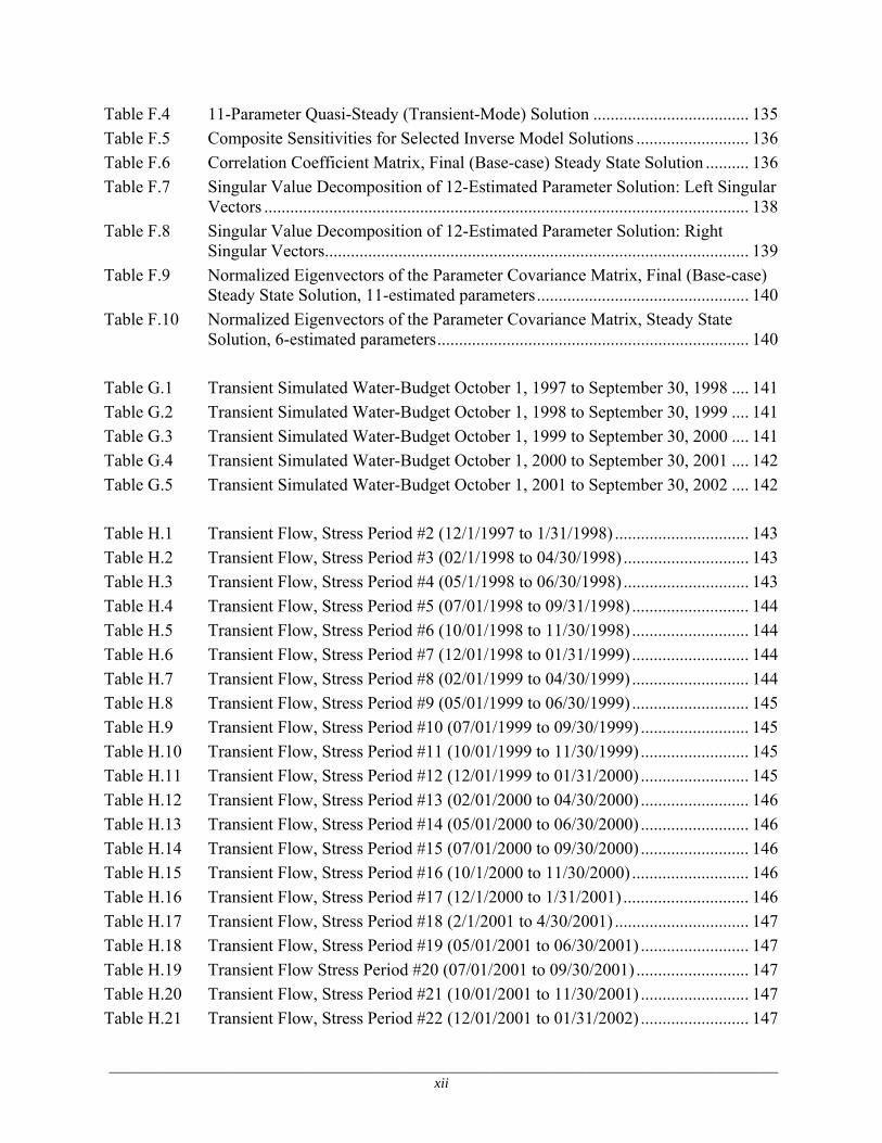
Table F.4 11-Parameter Quasi-Steady (Transient-Mode) Solution .................................... 135 Table F.5 Composite Sensitivities for Selected Inverse Model Solutions .......................... 136 Table F.6 Correlation Coefficient Matrix, Final (Base-case) Steady State Solution .......... 136 Table F.7 Singular Value Decomposition of 12-Estimated Parameter Solution: Left Singular
Vectors ................................................................................................................ 138 Table F.8 Singular Value Decomposition of 12-Estimated Parameter Solution: Right
Singular Vectors.................................................................................................. 139 Table F.9 Normalized Eigenvectors of the Parameter Covariance Matrix, Final (Base-case)
Steady State Solution, 11-estimated parameters................................................. 140 Table F.10 Normalized Eigenvectors of the Parameter Covariance Matrix, Steady State
Solution, 6-estimated parameters........................................................................ 140 Table G.1 Transient Simulated Water-Budget October 1, 1997 to September 30, 1998 .... 141 Table G.2 Transient Simulated Water-Budget October 1, 1998 to September 30, 1999 .... 141 Table G.3 Transient Simulated Water-Budget October 1, 1999 to September 30, 2000 .... 141 Table G.4 Transient Simulated Water-Budget October 1, 2000 to September 30, 2001 .... 142 Table G.5 Transient Simulated Water-Budget October 1, 2001 to September 30, 2002 .... 142 Table H.1 Transient Flow, Stress Period #2 (12/1/1997 to 1/31/1998) ............................... 143 Table H.2 Transient Flow, Stress Period #3 (02/1/1998 to 04/30/1998) ............................. 143 Table H.3 Transient Flow, Stress Period #4 (05/1/1998 to 06/30/1998) ............................. 143 Table H.4 Transient Flow, Stress Period #5 (07/01/1998 to 09/31/1998) ........................... 144 Table H.5 Transient Flow, Stress Period #6 (10/01/1998 to 11/30/1998) ........................... 144 Table H.6 Transient Flow, Stress Period #7 (12/01/1998 to 01/31/1999) ........................... 144 Table H.7 Transient Flow, Stress Period #8 (02/01/1999 to 04/30/1999) ........................... 144 Table H.8 Transient Flow, Stress Period #9 (05/01/1999 to 06/30/1999) ........................... 145 Table H.9 Transient Flow, Stress Period #10 (07/01/1999 to 09/30/1999) ......................... 145 Table H.10 Transient Flow, Stress Period #11 (10/01/1999 to 11/30/1999) ......................... 145 Table H.11 Transient Flow, Stress Period #12 (12/01/1999 to 01/31/2000) ......................... 145 Table H.12 Transient Flow, Stress Period #13 (02/01/2000 to 04/30/2000) ......................... 146 Table H.13 Transient Flow, Stress Period #14 (05/01/2000 to 06/30/2000) ......................... 146 Table H.14 Transient Flow, Stress Period #15 (07/01/2000 to 09/30/2000) ......................... 146 Table H.15 Transient Flow, Stress Period #16 (10/1/2000 to 11/30/2000) ........................... 146 Table H.16 Transient Flow, Stress Period #17 (12/1/2000 to 1/31/2001) ............................. 146 Table H.17 Transient Flow, Stress Period #18 (2/1/2001 to 4/30/2001) ............................... 147 Table H.18 Transient Flow, Stress Period #19 (05/01/2001 to 06/30/2001) ......................... 147 Table H.19 Transient Flow Stress Period #20 (07/01/2001 to 09/30/2001) .......................... 147 Table H.20 Transient Flow, Stress Period #21 (10/01/2001 to 11/30/2001) ......................... 147 Table H.21 Transient Flow, Stress Period #22 (12/01/2001 to 01/31/2002) ......................... 147

____________________________________________________________________________________________ xiii
Table H.22 Transient Flow, Stress Period #23 (02/01/2002 to 04/30/2002) ......................... 147

____________________________________________________________________________________________ Chapter 1 – Introduction 1
Chapter 1 - Introduction The Arizona Department of Water Resources (ADWR) has developed a regional groundwater flow model in the Santa Cruz Active Management Area (SCAMA) that covers a stretch of the effluent-dominated Santa Cruz River in southern Arizona. The model area is located in a unique hydrogeologic setting between the Nogales International Waste Water Treatment Plant (NIWTP) about 7 miles north of the Mexican border, and Elephant Head Bridge north of Arivaca Junction. See Figure 1.1. The hydrology associated with the inner Santa Cruz River Valley is characterized by complex stream-aquifer interactions, which includes periods of groundwater level rises, declines and quasi-steady state conditions. Outside the inner valley, groundwater development is currently insignificant, and the system is assumed to be in long-term equilibrium. Recognizing the differences between the Upper Santa Cruz River Basin and other groundwater basins in the Tucson AMA, the state legislature created the Santa Cruz AMA in 1994. Because of the distinct hydrologic conditions existing in the area, the legislature mandated that the Santa Cruz AMA preserve “safe-yield” conditions by “preventing long-term declines in local water tables”. The model was developed for understanding and quantifying the regional hydrologic system, and to provide guidance for the management of regional water resources in the Santa Cruz AMA. Originating in the San Rafael Valley in southern Arizona, the Santa Cruz River flows south into Sonora, Mexico, re-enters the U.S. about 5 miles east of Nogales and continues north past Tucson to the Gila River confluence where surface water flow is ephemeral. Until the late nineteenth century, surface water flowed perennially along the Santa Cruz River from the U.S.-Mexico border to Tubac. However, by the 1940’s groundwater pumpage, land-use changes and a prevailing dry climate had lowered water tables in the Santa Cruz River Valley. Since the 1970’s, treated effluent from the NIWTP has been continuously released into the river channel creating an additional source of recharge. Currently, release rates from the NIWTP average about 15,000 AF/YR and help sustain a prolific downstream riparian habitat. Groundwater stresses including pumpage and ET promote induced recharge when flood events occur in the Santa Cruz Valley. These changes have modified the hydrologic system and created the need for a management tool to help understand and predict hydrologic impacts of development. In recognition of this need, ADWR initiated a monitoring program in 1997 to guide development of a conceptual and numerical model (Nelson and Erwin, 2001).

____________________________________________________________________________________________ Chapter 1 – Introduction 2
Figure 1.1 Location of Study Area

____________________________________________________________________________________________ Chapter 1 – Introduction 3
Located in the semi-arid, southern Basin and Range province of southeastern Arizona, the upper Santa Cruz River Valley averages about 16 inches of precipitation per year, with higher rates outside the valley. See Table 3.1. Dependable summer monsoon rains, which are especially prevalent in southern Arizona, have generally been a reliable source of recharge to the system. Land surface elevations in the study area range from about 3,000 feet along the Santa Cruz River near Elephant Head Bridge near Arivaca Junction, to about 9,500 feet in the Santa Rita Mountains, located immediately east of the model domain. Groundwater-level elevations associated with the primary regional aquifers within the model area range from about 2,950 feet near Elephant Head Bridge to near 3,500 feet near the southern model boundary and east of Amado. Well-log and geophysical data show that three main Sub-areas comprise the upper Santa Cruz structural basin within the model area including the Amado, Tubac, and Rio Rico Sub-areas (Gettings and Houser, 1997). Three generalized basin-fill units are recognized including the: 1) Nogales Formation (Nog); 2) an upper basin-fill unit known as the Older Alluvium (Oal); and 3) a floodplain aquifer adjacent to the river of limited width and thickness, known and defined herein, as the Younger Alluvium (Yal). Primary inflows to the system include: 1) Recharge along the Santa Cruz River from natural and artificial (effluent from US and Mexico) sources; 2) tributary and mountain front recharge; 3) incidental agriculture recharge; and 4) subsurface groundwater inflow - predominately from the south. Primary outflows to the system include: 1) Seasonal evapotranspiration (ET) demand; 2) well pumpage from agriculture, municipal, industrial, and domestic sources; 3) underflow to the north; and 4) seasonal groundwater discharge to the Santa Cruz River between the NIWTP and Tubac. The regional flow direction is from south to north, and toward the inner Santa Cruz River Valley axis. Although periodic groundwater fluctuations occur, there haven’t been any significant, extended long-term (i.e. decadal) groundwater level trends recorded between 1982 and 2000 (Murphy and Hedley, 1984; Nelson and Erwin, 2001). Also, see Table D.6. Hydraulic head and flow data collected between 1997 and 2002 show that the system tends towards steady state conditions over winter, baseflow periods. During one of those winter periods (January – March, 2000), a groundwater basin sweep was conducted; the resulting composite hydraulic head distribution is shown in Figure 1.2.

____________________________________________________________________________________________ Chapter 1 – Introduction 4
Figure 1.2 Steady State Groundwater Levels, 2000

____________________________________________________________________________________________ Chapter 1 – Introduction 5
To better understand and quantify the interdependent hydrologic system, a finite-difference groundwater flow model (MODFLOW) was developed. The active model area covers about 152 miles2. The southern model boundary is located near the NIWTP, and extends 21 miles to near Arivaca Junction. The Tumacacori and Atascosa Mountains, and the San Cayetano and Santa Rita Mountains bound the model area to the west and east, respectively. The active model area covers the portions of the aquifer where most groundwater stresses occur in the Santa Cruz River Valley. Objective and Scope Objectives of this investigation include developing a groundwater flow model that will allow area stakeholders to 1) better understand the regional hydrologic system, and 2) make informed and objective water management decisions based on hydrology. This report presents simulated and observed hydraulic heads, flows and water budgets for steady state and transient conditions between 1997 and 2002. A pre-development steady state model was also developed for winter, baseflow periods, circa 1880. In addition, the post-development period between 1949 and 1959 was simulated in transient mode to examine model function over pre-effluent conditions. This report also discusses the model development process, model assumptions, limitations, strengths, weaknesses and suggestions for future modeling and data collection activities. Another fundamental objective of this project involved exploring alternative conceptual models and their reliability. Examining alternative conceptual models is an important aspect of groundwater modeling and is facilitated by inverse modeling (Poeter and Hill, 1997; Bredehoeft, 2003; Carrera et al., 2005; and Neuman and Wierenga, 2003). To accomplish these objectives, inverse models were developed to estimate model parameters including hydraulic conductivity and long-term natural recharge constrained over steady state, or quasi-steady conditions (e.g., winter, baseflow conditions 1997-2002). Automated calibration enabled the efficient evaluation of alternative conceptual models, including examination of alternative boundary conditions, basin-fill geometries, and hydraulic conductivity and recharge zones (see Chapter 4). In general, a parsimonious approach was followed in developing the models as advocated by the USGS (Hill, 1998). The alternative models were evaluated using the criteria outlined by the USGS (Hill, 1998) including: 1) Better fit; 2) weighted residuals that are more randomly distributed; and 3) more realistic parameter values. The final model presented herein attempts to balance these criteria. Although only one model is formally presented in this report (i.e. simulated hydrographs, budgets, parameter statistics, etc.), several other high-ranking alternative conceptual models are also discussed in Chapter 6. Overview of Water-Related History in the Model Area The upper Santa Cruz River Valley has a long and rich history due, in large part, to the availability of water along the Santa Cruz River. Human occupation in the upper Santa Cruz River Valley started as early as 1200 B.C. Prehistoric settlements in the Santa Cruz Valley, which include some of the oldest known water-controlled agricultural sites in North America, were centered on farming practices and the availability of reliable water along the river (Tellman, et.al.1997). Irrigated by ditches (acequias) before the arrival of the first Europeans as first documented by Eusebio Francisco Kino in 1689, crops including corn, squash and beans

____________________________________________________________________________________________ Chapter 1 – Introduction 6
were raised during the rainy season, and were also irrigated with surface water diverted along ditches to river terraces. In the late 17th century, Spaniards introduced crops such as winter wheat and new land-use practices including cattle grazing, which continue to this day. Historically, the Santa Cruz River flowed perennially from the U.S.-Mexico border to Tubac (Hendrickson, et al., 1984). Shallow water tables, dense riparian vegetation and even swampy conditions characterized this stretch of the river floodplain. Maps of Tubac, circa 1766, show a main acequia diverting and then redirecting return flow back to the Santa Cruz River (Meyer, 1984). In the 1840’s surface water flow along the Santa Cruz River was observed “disappearing” north of Tubac (Kessell, 1976), which, according to most historical accounts, appears to be the northern-most limit of reliable surface water flow. The long-term settlement of Tumacacori and Tubac suggest that these areas are somewhat buffered against periodic droughts. Groundwater pumpage from upper-basin fill aquifers have provided reliable water for crop irrigation in the Santa Cruz River Valley since the early 20th century. Intensive groundwater pumpage was partly responsible for declining water tables first observed in the 1930’s. Agricultural demand during the mid-20th century was significant and included cotton, a crop not currently grown in the area. Mid-century groundwater level declines were exacerbated by a relatively dry climate in southern Arizona observed between 1930 and 1960 (Webb and Betancourt, 1990). Other factors impacting groundwater level changes include the channelization and downcutting of the Santa Cruz River, evident from areal photographs taken in the 1950s (Parker, 1993). When streambed elevations change over time the altitude where surface water and groundwater flow interact also change, and thus impact groundwater levels (Webb and Leake, 2005). Additionally, the straightening (or channelization) of an otherwise naturally meandering stream, decreases the recharge potential to the underlying aquifer by reducing the extent of the wetted area. Geomorphologic changes, including channelization of the river in Santa Cruz County in the mid-twentieth century led to the removal of many pre-existing silt deposits bedded in the adjacent river terraces (Drewes, 1972b). Increases in extreme (fall and winter) flood recharge starting in the late 1960’s (into 2001), not only led to generalized increases in water table elevations, but also altered the channel morphology and streambed elevation. The hydrologic impacts to the groundwater system from impounding surface water flow from Sonoita Creek (Patagonia Lake, circa 1969), Agua Fria Canyon (Pena Blanca Lake, 1957), lining of Nogales Wash and possible upland watershed vegetation changes is not fully understood. However, it is also assumed that the regional groundwater flow regime, if previously altered from these modifications, has since re-equilibrated over the last couple of decades. Effluent discharge into the Santa Cruz River has created an additional source of recharge since 1972. Over recent periods, pumpage from municipal, industrial and domestic sources, as well as increases in evapotranspiration (ET) have offset traditional groundwater demands associated with agriculture and mining. As demand for municipal water supplies increased in Ambos Nogales, incidental surface water flow, spillage and run-off along the Nogales Wash, as well as leaks associated with the infrastructure leading into the NIWTP have provided a stable source of recharge near the southern model boundary. As a result, groundwater levels immediately south of the NIWTP have been relatively stable since the 1970s.

____________________________________________________________________________________________ Chapter 1 – Introduction 7
Today, the depth-to-water in the Santa Cruz River Valley is relatively shallow. Although periodic groundwater fluctuations occur, there haven’t been any significant, long-term (decadal) groundwater level trends observed in the model area between 1982 and 2002 (Murphy and Hedley, 1984; Nelson and Erwin, 2001; ADWR_GWSI, 2004). See Table D.6. Between 1997 and 2002, system outflows including well pumpage, ET demand, and subsurface outflows were effectively balanced by system inflows, including natural recharge (flood, baseflow, mountain front, and tributary recharge), artificial recharge (effluent and incidental agricultural), and subsurface inflow. During winter baseflow periods between 1997 and 2002, the system generally tended towards steady state conditions where the average precipitation rate (1997 – 2002) was similar to the long-term average rate, i.e. about 16 inches per year in the inner Santa Cruz River Valley. Since the spring of 2001 (through the spring of 2006) southern Arizona has been influenced by relatively dry conditions. This five-year “drought” has resulted in lower groundwater levels throughout most of the inner valley, especially in the northern and southern portions of the model area. Consequently, lower groundwater levels have reduced groundwater discharge between the NIWTP and Tubac. History suggests, however, that this is a temporary cycle, and that “wetter” periods will inevitably occur in the future. The active summer monsoon of 2006, which resulted in significant recharge in the southern portion of the model area, reflects the groundwater systems variability. Therefore, one of the underlying goals of this project is to better understand how the groundwater flow system is balanced (or imbalanced) - sometimes precariously - by both natural and artificial stresses.

____________________________________________________________________________________________ Chapter 1 – Introduction 8
Previous Investigations and Data Sources Many valuable hydrogeologic investigations have been conducted in the vicinity of the model area. The purpose of this section is to list some of the studies that have been particularly important towards understanding the system and developing the model. Important geologic investigations include those by Drewes (1972a; 1972b) and Cooper (1973). Drewes (1980) then went on to develop a regional-scale geologic map, much of which was used to define unit-types, and boundaries for the model. Simons (1974) developed a geologic map of the Nogales and Lochiel quadrangles in Santa Cruz County, which covers a portion of the model area. In the 1990’s, Gettings and Houser (1997) conducted geophysical investigations of the Upper Santa Cruz Sub-area in portions of Pima and Santa Cruz Counties. The inferred geologic structure, originally defined by Gettings and Houser (1997), was later refined by hydroGEOPHYSICS (2001). Sub-surface characteristics of the floodplain aquifer were investigated by Carruth (1995). The surficial geology and geomorphology near the Amado-Tubac area were reported by Youberg and Helmick (2001). Stream channel morphology and temporal changes in the general Tucson and north Santa Cruz County areas were examined by Parker (1993). Aldridge and Brown (1971) and Burkham (1970) investigated streamflow losses within the Upper Santa Cruz Sub-area, including infiltration rates for the Santa Cruz River and major tributaries. Osterkamp (1973) summarized groundwater recharge in the model area based on mountain front recharge rates provided by results of the electrical-analog model developed by Anderson (1972). In the 1990’s, the Arizona Department of Environmental Quality in co-operation with Friends of the Santa Cruz River (FOSCR) conducted a biological, water-quality, and stream infiltration study that concentrated on the effluent-dominated portion of the Santa Cruz River (Lawson, 1995). Effluent recharge to the upper Santa Cruz floodplain aquifer was investigated by the University of Arizona (Scott et al., 1996). ADWR (1994) and Stromberg et al (1993) investigated the effects of groundwater pumping and surface water diversion on riparian areas. Valuable investigations related to effluent recharge along the Santa Cruz River near Tucson were conducted by Lacher (1996). Starting in 1997, ADWR initiated a comprehensive monitoring program to collect various forms of data including hydraulic head, flow, and parameter data (Nelson and Erwin, 2001). Burtell (2000) provides estimates of transmission losses along the Santa Cruz River between Tubac and Elephant Head Bridge. An analysis of stage-discharge and width-discharge relations was conducted by Camp, Dresser & McKee as part of the Facilities Planning Process for Ambos Nogales (CDM, 1999). Arizona State Parks has provided surface water flow discharge measurements in the general Sonoita Creek area (AZ State Parks, 2006). Shamir et.al.(2005), provides a comprehensive analysis of surface water flow along the Santa Cruz River near Nogales. The Upper Santa Cruz Sub Valley was originally modeled by Anderson (1972) using electric analogue techniques. A numerical groundwater flow model was developed for the Upper Santa Cruz Sub-area by Travers and Mock (1984) and later refined by Hanson and Benedict (1994). McSparran (1998) evaluated the optimization of waste effluent allocation in the Santa Cruz AMA through a MODFLOW modeling study. Currently, ADWR is completing two groundwater flow models adjacent to this study. One model covers the Tucson AMA, which overlaps a small

____________________________________________________________________________________________ Chapter 1 – Introduction 9
portion of this model area (Mason and Bota, 2006). Another model covers the Santa Cruz River and aquifer system between the international border and the NIWTP located immediately south of this model area; this area is also known as the micro-basin area (Erwin, in press). Numerous investigators have evaluated hydrogeologic and hydraulic conditions within the model area. Aquifer parameters in the vicinity of the model area have been evaluated by many different sources, including Halpenny (1982, 1983, 1984, 1985, 1986, 1987, and 1989), Groundwater Resources Consultants (1997); Clear Creek Associates (2002a and 2002b); Brown and Caldwell (2003); Manera, (1980); Environmental Resource Consultants (1996); University of Arizona (1960); Dickens, C.M. (2004); and Cella Barr (1990); Errol L. Montgomery & Associates (2005). Specific capacity data in the model area was obtained from ADWR’s GWSI database (ADWR_GWSI, 2004). Groundwater level data used as hydraulic head calibration targets over steady state and transient periods are located in the GWSI database (ADWR_GWSI, 2004). Many of the surface water flow measurements and groundwater levels reported in Nelson and Erwin (2001) were used as baseflow calibration targets. Murphy and Hedley (1984) developed a groundwater elevation contour map of the regional aquifer system measured for groundwater conditions in early 1982. Recorded groundwater pumpage was supplied by ADWR’s Registry of Groundwater Rights (ADWR_ROGR, 2004) database. Continuous effluent discharge rates from the NIWTP were recorded by International Boundary and Water Commission (IBWC, 1995-2004). The USGS has been collecting surface water flow data at Tubac and Amado since 1995 and 2004, respectively (USGS_Ama, 2004; USGS_Tub, 1995-2004). Long-term surface water flow data has been collected near Nogales (USGS_Nog, 2004). The Friends of the Santa Cruz River provided additional surface water flow measurements along the river. Estimates for evapotranspiration (ET) losses were investigated by Masek (Masek, 1996). Precipitation data collected at various sites in the vicinity of the model area were obtained from the AZClimate (2004) and NOAA (2005).

____________________________________________________________________________________________ Chapter 2 – Hydrogeology 10
Chapter 2 - Hydrogeology The model area is located in the upper Santa Cruz River valley in the southern Basin and Range province of southeastern Arizona (Nations and Stump, 1981). Mountain ranges found in the model area are generally fault-bounded and include the Santa Rita and San Cayetano Mountains to the east, and the Tumacacori and Atascosa Mountains to the west. Sediment-filled basins began to form about 17 Ma in southeastern Arizona as a result of dominantly east-northwest/west-southwest directed crustal extension (Gettings and Houser, 1997). Most groundwater occurs within the basin-fill units including the: 1) Nogales Formation (Nog) unit, also known as gravel of Nogales, or lower basin fill; 2) the Older Alluvium (Oal) unit, also known as upper basin fill; and 3) the Younger Alluvium (Yal) unit also identified as the floodplain aquifer, river facies, Qtal, Qal, younger surficial deposits, and stream channel alluvium. The Yal has also been classified as an upper-basin fill unit. Figures 2.1 and 2.2 show conceptualized geologic cross-sections in the Amado and Rio Rico Sub-areas, respectively. Geophysical investigations show three Sub-areas are associated with the Nogales Formation and Older Alluvial unit in the model area (See Figure 1.2). From north to south, the Sub-areas include the Amado, Tubac, and Rio Rico sub basins (Gettings and Houser, 1997; HydroGEOPHYSICS, 2001). Because the basin-fill units dominate the groundwater flow regime in the model area (i.e. flood and effluent recharge; pumping and ET demand), the Older and Younger Alluvium units and their associated aquifers are the primary focus of this modeling investigation. Groundwater also exists within fractured and weathered volcanic, granitic, metamorphic, and sedimentary rocks that bound the basin-fill units. Hardrock areas associated with the surrounding mountain ranges have not been directly included in the groundwater flow model; however, hardrock areas can contribute mountain-block flow to the basin-fill units. Therefore an undifferentiated component of mountain front recharge originates from source areas outside the active model domain, which ultimately flow into the basin-fill aquifers. For convenience, the surrounding hardrock areas have been labeled as “undifferentiated bedrock” on maps. For a thorough description of rock types within the model area see Drewes (1972a; 1972b; 1980), and Simons (1974).

______________________________________________________________________________________________________________________________ Chapter 2 – Hydrogeology 11
Figure 2.1 Generalized Hydrogeologic Cross-Section near Amado

_______________________________________________________________________________________________________________________________ Chapter 2 – Hydrogeology 12
Figure 2.2 Generalized Hydrogeologic Cross-Section near Rio Rico

____________________________________________________________________________________________ Chapter 2 – Hydrogeology 13
Geologic Structure Along the 21-mile valley length, the Santa Cruz Valley ranges in width from about 5 to 8 miles. The valley experienced minor to moderate lateral extension and faulting during the late Cenozoic period. Bouguer gravity and aeromagnetic anomaly maps indicate that the Mt. Benedict fault, which controls the structure of the river south of the NIWTP, continues beneath the basin fill to the north (Gettings and Houser, 1997). The Mt. Benedict fault separates the Rio Rico and Tubac sub basins, and data suggests that the fault controls the location of the Santa Cruz River north of the NIWTP (Gettings and Houser, 1997). Drewes (1980) and Gettings and Houser (1997) both show a fault (which will be referenced herein as the Santa Cruz River fault) west of the Santa Cruz River. The Santa Cruz River fault crosses the Mt. Benedict fault near Tumacacori and continues north. Regional-scale playa and lacustrian facies have not been observed within the inner valley, suggesting that the basin was never closed during deposition of the lower and upper basin fills, and that the system was drained by a north or south-flowing axial stream (Gettings and Houser, 1997). Examination of groundwater data from shallow and deep perforated wells show correlated head responses, further suggesting that there are no significant vertical gradients within the inner valley system (ADWR_GWSI, 2004). Numerous faults exist along the eastern portion of the basin fill units within the San Cayetano and Santa Rita Mountains. The San Cayetano fault separates the Grosvenor Hills block to the east, and the San Cayetano block to the west. The Grosvenor Hills block has dropped an estimated 1,000 to 2,500 feet along the southern part of the San Cayetano fault. Westward tilting is indicated by westwards dips of the Nogales Formation which overlap volcanic rocks along the southern portion of the San Cayetano fault (Drewes, 1972a). The flexure associated with the Nogales Formation near the Glove mine (i.e., upper reaches of Cottonwood Canyon) indicates that additional movement probably occurred along the fault near the end of the Tertiary (Drewes, 1972a). Many of the faults along the Santa Rita and San Cayetano mountains have been truncated by the Oal unit (Drewes, 1972b). Faults and fractures can act as conduits for groundwater recharge and discharge. Preferential pathways for groundwater flow along fault and fracture zones in contact with basin fill units are assumed to be a direct hydraulic connection to the inner valley aquifer system. For example along the western foothills of the Santa Rita Mountains, Agua Caliente Springs discharges groundwater (Halpenny, 1987) along the Agua Caliente/Montosa thrust fault zones. Complex hydraulic conditions also exist near Sopori Springs where groundwater “upwells” from a Triassic conglomerate (Halpenny, 1989). Other springs have been noted in the vicinity of the model area and include Aliso Springs, Puerto Springs, Toros Springs, Chivas Springs, and Fresno Springs. Hydraulic Properties of the Basin-filled Aquifers The purpose of this section is to provide an overview of the hydraulic properties associated with the three basin-fill aquifers, including the Nogales Formation, the Older Alluvial aquifer, and the Younger Alluvial aquifer. The geometrical boundaries associated with the two lower basin-fill units, including the Nogales Formation and the Older Alluvium, were based on geophysical
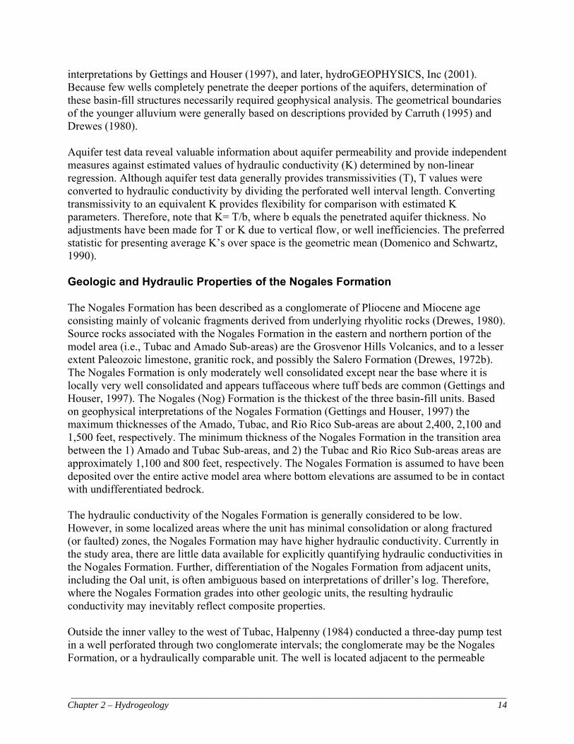
____________________________________________________________________________________________ Chapter 2 – Hydrogeology 14
interpretations by Gettings and Houser (1997), and later, hydroGEOPHYSICS, Inc (2001). Because few wells completely penetrate the deeper portions of the aquifers, determination of these basin-fill structures necessarily required geophysical analysis. The geometrical boundaries of the younger alluvium were generally based on descriptions provided by Carruth (1995) and Drewes (1980). Aquifer test data reveal valuable information about aquifer permeability and provide independent measures against estimated values of hydraulic conductivity (K) determined by non-linear regression. Although aquifer test data generally provides transmissivities (T), T values were converted to hydraulic conductivity by dividing the perforated well interval length. Converting transmissivity to an equivalent K provides flexibility for comparison with estimated K parameters. Therefore, note that K= T/b, where b equals the penetrated aquifer thickness. No adjustments have been made for T or K due to vertical flow, or well inefficiencies. The preferred statistic for presenting average K’s over space is the geometric mean (Domenico and Schwartz, 1990). Geologic and Hydraulic Properties of the Nogales Formation The Nogales Formation has been described as a conglomerate of Pliocene and Miocene age consisting mainly of volcanic fragments derived from underlying rhyolitic rocks (Drewes, 1980). Source rocks associated with the Nogales Formation in the eastern and northern portion of the model area (i.e., Tubac and Amado Sub-areas) are the Grosvenor Hills Volcanics, and to a lesser extent Paleozoic limestone, granitic rock, and possibly the Salero Formation (Drewes, 1972b). The Nogales Formation is only moderately well consolidated except near the base where it is locally very well consolidated and appears tuffaceous where tuff beds are common (Gettings and Houser, 1997). The Nogales (Nog) Formation is the thickest of the three basin-fill units. Based on geophysical interpretations of the Nogales Formation (Gettings and Houser, 1997) the maximum thicknesses of the Amado, Tubac, and Rio Rico Sub-areas are about 2,400, 2,100 and 1,500 feet, respectively. The minimum thickness of the Nogales Formation in the transition area between the 1) Amado and Tubac Sub-areas, and 2) the Tubac and Rio Rico Sub-areas areas are approximately 1,100 and 800 feet, respectively. The Nogales Formation is assumed to have been deposited over the entire active model area where bottom elevations are assumed to be in contact with undifferentiated bedrock. The hydraulic conductivity of the Nogales Formation is generally considered to be low. However, in some localized areas where the unit has minimal consolidation or along fractured (or faulted) zones, the Nogales Formation may have higher hydraulic conductivity. Currently in the study area, there are little data available for explicitly quantifying hydraulic conductivities in the Nogales Formation. Further, differentiation of the Nogales Formation from adjacent units, including the Oal unit, is often ambiguous based on interpretations of driller’s log. Therefore, where the Nogales Formation grades into other geologic units, the resulting hydraulic conductivity may inevitably reflect composite properties. Outside the inner valley to the west of Tubac, Halpenny (1984) conducted a three-day pump test in a well perforated through two conglomerate intervals; the conglomerate may be the Nogales Formation, or a hydraulically comparable unit. The well is located adjacent to the permeable

____________________________________________________________________________________________ Chapter 2 – Hydrogeology 15
inner valley aquifer material. Raw pump test data provided by Halpenny (1984) were re-evaluated by ADWR using AQTESOLV (Duffield, G.M., Rumbaugh, J.O., 1991). The analysis shows that the drawdown response closely matches the leaky-aquifer solutions of Hantush and Jacob (1955), and Moench (1985). Interpretation of aquifer test data indicates that the well is perforated in an aquifer(s) having relatively low transmissivity; however, the data also suggests that the aquifer receives leakage from an adjacent source. The physical location of the well suggests that the continuous source of leaky water might originate from the relatively permeable aquifer material located immediately to the east - in the inner Santa Cruz River Valley. The hydraulic conductivity of the conglomerate unit (Nogales Formation) was determined to be 0.30 feet/day, and 3.0 feet/day, based on the solutions of Hantush and Jacob (1955), and Moench (1985), respectively. Two aquifer tests have been conducted in the Nogales Formation, or hydraulically similar unit, south of the model area (Halpenny, 1985; Manera, 1980). Results show low transmissivities are associated with both perforated zones. The inferred hydraulic conductivities associated with (D-24-15) 16bdd and (D-24-15) 08ada were 0.43 feet/day and 0.17 feet/day, respectively. For more on these results see Erwin (in press). For comparative purposes, Freeze and Cherry (1979) list the range of hydraulic conductivity associated with sandstone as between 0.000134 feet/day and 1.34 feet/day. For reference, the calibrated transmissivity of the Pantano Formation - a unit similar to the Nogales Formation north of the model area - was determined to be about 1,200 feet2/day (Mason and Bota, 2006). Assuming the saturated thickness of the Nogales Formation is about 2,000 feet near Amado, the hydraulic conductivity would be on the order of about 0.5 feet/day. Geologic and Hydraulic Properties of the Older Alluvial Unit Primarily an alluvial basin-fill deposit comprised of gravel, sand, and clay of Pliocene and Pleistocene age, the Oal unit also includes colluvium and landslide deposits (Drewes, 1980). The Oal unit is slightly, to moderately consolidated with some areas indurated enough to form cliffs (Simons, 1974). Thicknesses associated with the Oal unit generally range from a few meters, where it overlaps onto bedrock or the Nogales Formation, to about 850-1,200 feet (260-365 m) in the Amado Sub-area (Drewes, 1980; Gettings and Houser, 1997). Contact between the Nogales Formation and the Oal Unit is gradational over an interval of about 160 feet (50 m), and is marked by a decrease in consolidation and increase in the variety of sediment clasts from the Nog unit upwards toward the Oal unit (Gettings and Houser, 1997). Geophysical investigations and well log data show that the Oal unit widens and thickens from the south to the north (Gettings and Houser, 1997). The Oal unit is overlain by terrace and pediment deposits (Drewes, 1972b). Maximum thicknesses associated with the older alluvial unit in the Amado, Tubac, and Rio Rico Sub-areas are approximately 900, 300 and 500 feet, respectively (Gettings and Houser, 1997). The minimum saturated thickness of the Oal aquifer in the transition area between the 1) Amado and Tubac Sub-area, and 2) the Tubac and Rio Rico Sub-areas are approximately 130 and 60 feet, respectively (Gettings and Houser, 1997). Although there has been a relatively large number of aquifer and pumping tests conducted in the Older Alluvial aquifer, most were conducted within the inner Santa Cruz River Valley. For statistical purposes, aquifer test data collected

____________________________________________________________________________________________ Chapter 2 – Hydrogeology 16
from nearby areas were also included in the evaluation. These areas include the Potrero Sub-area - south of the Rio Rico Sub-area, and in the northern portion of the Amado Sub-area near Canoa, south of Green Valley. Inferred values of hydraulic conductivity identified in the Potrero Sub-area and the Amado Sub-area near Canoa are assumed to be hydraulically comparable to properties found in the Rio Rico and Amado Sub-area near the Amado model area, respectively; examination of groundwater levels suggest these areas are in direct hydraulic connection. Aquifer test results show that the older alluvial aquifer is spatially heterogeneous over the model area. Hydraulic conductivity values range from less than 1 foot/day to greater than 50 feet/day. Available data suggest that at least four distinctive Oal hydraulic conductivity zones exist in the model area including 1) the inner Santa Cruz Valley in the Tubac and Amado Sub-areas (Koal_North); 2) an area east of Tubac (Koal_Tub_East); and 3) the Rio Rico and Potrero Sub-areas area (Koal_RR). Steep hydraulic gradients east of Amado indicate that another zone of relatively low hydraulic conductivity exists (Koal_Northeast). Based on aquifer test and specific capacity data, the Koal_North zone shows moderately-high hydraulic conductivity. The geometric mean associated with Koal_North is about 30 feet/day. The western extent of Koal_North approximately parallels the Santa Cruz River fault suggesting that the aquifer hydraulics may be a function of the structural relationships in this area. Available data suggest that the eastern extent of the permeable inner valley zone approximately parallels the inner Santa Cruz River Valley. East of Tubac, the hydraulic conductivity of Koal_Tub_East has a geometric mean of about 5.0 feet/day. In the Rio Rico and Potrero Sub-areas, Koal_RR has a geometric mean hydraulic conductivity of about 10 feet/day. Hydraulic conductivity data does not exist for the area east and northeast of Amado; however, the steep hydraulic gradient suggests that the K’s are very low. For reference, Freeze and Cherry (1979) list the range of hydraulic conductivity for silty-sand and clean sand between 0.134 and 1,340 feet/day. Acting on results of an alternative conceptual model that suggest a high-K feature in the northwestern portion of the Rio Rico Sub-area, ADWR conducted a short-term reconnaissance aquifer test in February 2006. Results of the aquifer test show extremely high hydraulic conductivity (200 – 2,000 feet/day) in this area - consistent with the alternative model solution. See Appendix B. Gettings and Houser (1997) show an inferred fault along this area, and the hydraulic properties of the local aquifer may reflect fractured flow in this area. The high-K feature is located on the Atascosa Ranch, and the owner indicated that the well was intentionally placed near a lineament (personal communication with J.D. Lowell, 2006). The areal extent of this high-K zone and its function in the regional groundwater flow system remain unknown. For more discussion about this alternative conceptualization see Chapters 3 and 6. Geologic and Hydraulic Properties of the Younger Alluvial Unit The Yal unit of late Pleistocene to Holocene age consists of well-sorted and uniform deposits of sub-rounded to rounded cobbles that have little silt and clay (Drewes, 1972b). Driller logs and surface out-crops indicate the thickness of the Yal unit varies from 30 to about 150 feet (Carruth, 1995). The Yal unit is typically 1-3 miles in width, and its lateral extent is irregular (Drewes, 1972b). Because of its well-sorted and course-grained characteristics, the Yal unit has high transmissivity and hydraulic conductivity; aquifer test data show this is especially true in the Rio

____________________________________________________________________________________________ Chapter 2 – Hydrogeology 17
Rico Sub-basin. For example, shallow wells perforated in the Yal aquifer near Rio Rico can produce discharge rates exceeding 4,000 GPM with relatively little drawdown (ADWR_GWSI, 2004). Schwalen and Shaw (1957) even reported a well near Rio Rico produced over 5,000 GPM, the highest yield of any well in the Santa Cruz Valley south of Rillito. Youberg and Helmick (2001) provide detailed descriptions of the surficial geology. Aquifer test and specific capacity data were used to characterize the spatial distributions of Yal hydraulic conductivity zones. Based on available data, two generalized Yal subsurface hydraulic zones have been identified in the 1) Tubac and Amado area, and 2) in the Rio Rico area. Aquifer test and specific capacity data show extremely high values of hydraulic conductivity in the Rio Rico Sub-area where the geometric mean K is about 600 feet/day (Kyal_RR). In the northern portion of the model area, the hydraulic conductivity appears to be lower than in the Rio Rico Sub-area. Accordingly, the geometric mean in the Tubac and Amado area averages about 170 feet/day (Kyal_North). In the northern portion of the study area, independent modeling investigations show calibrated K values are reasonably consistent with the geometric mean of Kyal_North, and range from 100 and 150 feet/day (Hanson and Benedict, 1994; Mason and Bota, 2006). Freeze and Cherry (1979) list the range of hydraulic conductivity associated with clean sand and gravel between 13.4 and 134,000 feet/day. Summary of Hydraulic Conductivities in Model Area A summary of observed hydraulic conductivities are provided in Table 2.1. Appendix B lists the individual aquifer test and specific capacity results. For location of individual aquifer tests and specific capacity data see Figure 2.3. Available data suggests that there are distinctive Yal and Oal hydraulic conductivity zones in the Rio Rico/Potrero Sub-area, and the Tubac/Amado Sub-area. Geologic data suggests that the Rio Rico and Tubac/Amado Sub-areas may have had distinctive depositional environments resulting in unique hydraulic properties. Older volcanic detritus, including the Grovenor Hills Volcanics that eroded off the Santa Rita Mountains are not present in the Rio Rico Sub-area; thus distinctive compositions exist between the Rio Rico and Tubac/Amado Sub-areas (Personnel communication with Mark Gettings, USGS Geophysicist, 2004). These differences appear to be reflected in the distinctive hydraulic conductivity values found in these areas. Also of note is the fact that the Santa Cruz River fault crosses the Mt. Benedict fault just south of Tumacacori. Geologic and hydraulic data suggest these faults might be, at least partially, responsible for the stable groundwater levels observed in the northern portion of the Rio Rico Sub-area and in the Tubac Sub-area, as well as groundwater discharge along the river between Peck Canyon and Tumacacori over winter baseflow periods (1992-2002).

____________________________________________________________________________________________ Chapter 2 – Hydrogeology 18
Figure 2.3 Location of Aquifer Tests

____________________________________________________________________________________________ Chapter 2 – Hydrogeology 19
Table 2.1 Statistical Summary of the Hydraulic Conductivities ZONE *GEOMETRIC MEAN
K ARITHMETIC MEAN
K STANDARD DEVIATION MEDIAN K
Knog 0.50 0.763 0.81 (3 sites) 0.426 Koal_North 29.8 58.0 57 (10 sites) 42 Koal_Tub_East 4.57 6.33 4.73 (4 sites) 5.92 Koal_RR 11 14.7 13.8 (10 sites) 12.1 Kyal_North 168 246 223 (7 sites) 170 Kyal_RR 570 1000 753 (6 sites) 1,150 *Preferred statistic for average K over space (Domenico and Schwartz, 1990). All units feet/day.
At the time of this writing there haven’t been any aquifer tests conducted to determine vertical hydraulic conductivities in the model area. Halpenny (1983) suggests that the vertical hydraulic conductivity of the alluvial aquifers is one to two orders of magnitude less than horizontal hydraulic conductivity. As previously mentioned, no lacustrian deposits have been observed in the field to date, nor have any significant vertical hydraulic gradients been observed in the inner Santa Cruz Valley within the model area. This information suggests that regional-scale confining layers probably do not exist within the inner Santa Cruz River Valley. Corroborating this, recent drilling and aquifer testing reveal that the Oal aquifer operates under unconfined conditions in the Rio Rico sub-area (Errol L. Montgomery & Associates, Inc. 2005). Hydraulic Storage Properties The specific yield, Sy, is defined as the volume of water that an unconfined aquifer releases from storage per unit surface area of aquifer per unit decline in the water table (Freeze and Cherry, 1979). Based on an aquifer test conducted in Rio Rico, the specific yield associated with the Yal aquifer was determined to be 19% using Neuman’s (1975) solution (See Appendix B). Gravity studies conducted southeast of the model area near Nogales’ Santa Cruz River well field show composite Sy values, associated with the Yal and Oal aquifers, between 8.6-14.4% (Nelson and Erwin, 2001). The calibrated specific yield value associated with the unconfined floodplain aquifer in the northern portion of the Tucson AMA groundwater flow model was 16-20% (Mason and Bota, 2006; Hansen and Benedict, 1994). Hanson and Benedict (1994) list the Sy associated with older alluvial sediments at between 10% and 13%. The calibrated value of specific yield assigned to deeper portions of the Tucson Basin, including the Pantano Formation, are calibrated at 5% (Hanson and Benedict, 1994). The deeper aquifers of the Tucson Basin, including the Pantano Formation, are assumed to have hydraulic properties comparable to those of the Nogales Formation. Thus, based on aquifer test data, gravity data, and previously calibrated models, specific yield values associated with the Yal aquifer, Oal l aquifer and Nogales Formation are assumed to be 18%, 10%, and 5%, respectively. For comparative purposes, Freeze and Cherry (1979), list the usual range of specific yield between 1 and 30%. Specific storage, Ss, is defined as the volume of water that a unit volume of aquifer releases from storage under a unit decline in hydraulic head. The storage coefficient, S, where S = Ss*b, and b represents the aquifer thickness, ranges between 0.005 and 0.00005 (Freeze and Cherry, 1979). Based on aquifer test results (See Appendix B), a representative Ss value for the basin-fill aquifers is assumed to be 6.67E-6 ft-1.

____________________________________________________________________________________________ Chapter 3 – Regional Groundwater Flow System Conceptual Model 20
Chapter 3 - Regional Groundwater Flow System Conceptual Model System Inflows Inflows to the system have been separated into five general components including: 1) mountain front recharge (MFR); 2) Tributary (Trib) recharge; 3) recharge along the Santa Cruz River; 4) incidental agriculture recharge, and 5) sub-surface inflow. Differentiating recharge components enables the individual calibration and understanding of the specific recharge properties and their associated reliability. Mountain Front Recharge Along mountain front areas, surface water flow from precipitation infiltrates into the subsurface. Groundwater recharge along mountain front areas (MFR) migrates laterally towards the inner Santa Cruz River Valley. Faults and fractures in the vicinity of the model area (Drewes, 1972a; Gettings and Houser, 1997) also provide mechanisms for groundwater recharge and discharge. Groundwater level contour maps show lateral flow directed towards the valley axis (Nelson and Erwin, 2001; Murphy and Hedley, 1984; Hansen and Benedict, 1994).
Conceptual estimates of MFR in the model area total about 5,000 AF/YR (Osterkamp, 1973). Higher rates of MFR are assumed to occur at higher elevations due to orographic-based precipitation. Accordingly, it is assumed that higher rates of recharge occur along the windward (i.e., west and south) side of the Santa Rita Mountains, which exceed 9,000 feet, than along lower elevation valley-floor areas; this assumption is consistent with other studies including Osterkamp (1973); Travers and Mock (1984); and Hansen and Benedict (1994). See Figure 4.1 for distribution of MFR. Measuring recharge along all tributary and mountain front areas over indefinite “long-term” periods is highly impractical. Examination of long-term precipitation rates, however, can provide an indirect measure of recharge variability in remote mountain front and tributary areas, as well as recharge along the Santa Cruz River. Table 3.1 shows the mean long-term and recent (1997-2002) precipitation rates recorded at various locations around the model area (AZClimate, 2004; NOAA, 2005). Note that average precipitation rates recorded over the transient simulation period (1997-2002) are similar to long-term average rates.

____________________________________________________________________________________________ Chapter 3 – Regional Groundwater Flow System Conceptual Model 21
Table 3.1 Precipitation Rates in General Model Area
LOCATION LONG-TERM ANNUAL AVERAGE
PRECIPITATION RATE, STANDARD DEVIATION σ
RECENT PERIOD (1997- 2002) AVERAGE ANNUAL
PRECIPITATION HIGH AND LOW RATES
Tumacacori *1948 – 2004: 15.7”, σ 5.1” a15.1”: High 19” Low 9.3” Nogales 6 N Old Nogales Nogales
*1954 – 2004: 17.4”, σ 5.0” *1901- 1946: 15.7”, σ 4.1” *1948- 1983: 16.6”, σ 4.2”
15.7”: High 26” Low 8.0”
Santa Rita Experimental Range *1950 – 2004: 22.1”, σ 5.1” 21.1”: High 25” Low 18.0” Coronado Natl. Monument *1960 – 2004: 20.6”, σ 5.0” 20.1”: High 31” Low 13” Canelo 1NW (near Patagonia) *1910 – 2003: 18.1”, σ 4.1 17.1”: High 26” Low 11” Arivaca **1971-2000: 18.7” 17.7”: High 25” Low 12” Patagonia **1971-2000: 18.3” 17.6”: High 23” Low 10” aMissing more than 34 days of data; Source: *AZClimate, 2004; **NOAA, 2005. All units in inches.
Tributary Recharge Groundwater recharge along major tributaries provides an important source of water to the basin-fill aquifers. Permeable streambed sediments associated with the tributaries provide direct hydraulic mechanisms for groundwater recharge. Major tributary confluences occur every few miles along the river and provide continuous subsurface flow into the inner valley areas. During the 1998 El Nino and 1998 and 1999 monsoon periods, net infiltration was observed along major tributaries including Sonoita Creek, Agua Fria, and Peck Canyons. For example following the 1998 El Nino events, approximately 10 cfs of surface water flow was observed in Sonoita Creek about 2-3 miles upstream of its confluence with the Santa Cruz River, (D-23-13) 01aaa, however no surface water flow was observed at the Santa Cruz River confluence. As with MFR, tributary recharge estimates reflect long-term average rates. Conceptual estimates for tributary recharge is assumed to be 6,600 acre-feet/year (Aldridge and Brown, 1971; Halpenny and Halpenny, 1989). For conceptual estimates, see Table 4.2. Recharge along the Santa Cruz River: Flood and Effluent Recharge Stream recharge along the main stem of the Santa Cruz River has a significant impact on the groundwater flow regime in the Santa Cruz River Valley. Currently, both natural recharge (i.e. flood, baseflow) and artificial recharge (effluent recharge, incidental agricultural recharge from runoff) occur within the model area. Recharge along the Santa Cruz River is a function of many interdependent factors including the hydraulic properties of the aquifer, the geometrical boundaries of the system, bank storage, storage availability of the aquifer, demands such as ET and pumpage, the characteristics of flow events, i.e., flood frequency, duration, magnitude, and timing and season, and streambed properties including the saturated and unsaturated hydraulic streambed conductivity. Treated Effluent Recharge and Baseflow conditions Since the early 1970s, treated effluent from the NIWTP has been continuously released into the Santa Cruz River near the Nogales Wash confluence, and augments natural flow along the Santa Cruz River. Effluent recharge, along with increases in major winter flood recharge events

____________________________________________________________________________________________ Chapter 3 – Regional Groundwater Flow System Conceptual Model 22
between 1960’s and 2001, increased ET demand and reduced groundwater pumpage, dechannelization of the river (i.e. conversion back to a more naturally-meandering, aggregating, widening streambed channel), lining of the upgradient Nogales Wash and possible upland vegetation changes have created a new dynamic flow regime in the valley. Effluent discharge rates from the NIWTP currently range from about 12,000 to 15,000 AF/YR (IBWC, 1997-2002). Effluent recharge over baseflow periods between the NIWTP and Tubac can be limited because of high water tables (hydrostatic conditions, i.e. where the water table and streambed elevation are nearly equal) and groundwater discharge along this reach; this was especially true over winter periods between 1992 and 2002. Also, sedimentation and growth of a thin, yet relatively impermeable, biological film on the stream bottom can form a clogging layer immediately downstream from the NIWTP. This clogging layer can effectively prohibit effluent recharge along the river over non-flood, baseflow periods. If storage space is available, large flow events have the potential to scour off the clogging layer, and thus facilitate recharge. In the absence of scouring flood-pulses, the clogging layer redevelops. The hydraulic nature of the clogging layer has also been reported in the Tucson area (Lacher, 1996) where hydrologic conditions are similar. Seepage measurements recorded between 1997 and 2002 show that most baseflow/effluent recharge occurs north of Tubac (Nelson and Erwin, 2001). Observation data collected between 1997-2001 shows that recharge rates between Tubac and Elephant Head Bridge average about 19 cfs over winter (non-flood) periods. Also see Table E.4. Flood and Recessional Flow Recharge Between 1997 and 2002 the median and mean flow at Tubac was 21 and 46 cfs, respectively, reflecting the impact of flood flow along the river (USGS_Tub, 2004). Between 1997 and 2002, there were four significant flood recharge events including the 1998 El Nino (primarily resulting in recharge between February and April, 1998), two active monsoons periods in 1998 and 1999, and an extreme flood recharge event in October and November of 2000, which also resulted in significant recessional flow and subsequent recharge into early 2001. Each of these four flood events occurred in between dry periods. Long-term flow records exist at Buena Vista (USGS, 09480500); however this gauge does not reflect flow contributions from tributaries such as Sonoita Creek, Nogales Wash, Agua Fria, Peck and Josephine Canyons. Drainage areas for the Nogales and Tubac gauges are 533 and 1,209 miles2, respectively, and their flow magnitudes and “signatures” can be quite different. Historical data from Buena Vista, and the Charleston USGS gauge along the San Pedro River (which has a similar watershed area as Tubac), suggest that the model area has a long history of significant, yet variable, flood activity (Webb and Betancourt, 1990). Shamir et al (2005) provides a comprehensive analysis of historical surface water flows along the Santa Cruz River near Nogales. There appear to be two general modes of flood recharge in the inner valley system. One fairly dependable and important source of recharge is associated with short-duration high magnitude floods, typical during the North American Monsoon (July through September). Active monsoon seasons with frequent precipitation and channel flow induce appreciable recharge, as was the case in 1998 and 1999 (and 1954, 1955, 1983, 1984, 1990, 2006 and many other years). The other general mode of flood recharge occurs over cooler fall, winter and spring periods. Precipitation from slow-moving pacific frontal storms or dissipating tropical storms (sometimes

____________________________________________________________________________________________ Chapter 3 – Regional Groundwater Flow System Conceptual Model 23
associated with cut-off lows) can generate significant direct recharge, as well as antecedent recharge from recessional flow for many months following the primary precipitation event(s). Although infrequent in nature, recharge from significant fall/winter flood events can effectively fill inner valley aquifers, even across the broader expanses of the inner valley, as was the case in 1967-68, 1983-84, 1993-94 and 2000-01. See Nelson and Erwin (2001) for flood recharge hydrographs of the significant 2000-01 flood recharge event. For either summer or non-summer flood events, it appears that significant flow magnitudes are required to remove the clogging layer downstream from the NIWTP, thus allowing recharge. Incidental Agriculture Recharge According to a recent study the calculated irrigation efficiency ranges from 44 percent to more than 100 percent, or deficit irrigation (Scott, et al., 1996). In 1995, irrigated crop evapotranspiration from the NIWTP to Tumacacori was determined to be 5,133 acre-feet (Unland, et al, 1997). The agricultural-related groundwater pumpage between the NIWTP and Tumacacori in 1995 was 6,950 acre-feet (ADWR_ROGR, 2004), thus yielding an irrigation efficiency of about 75%, or an incidental recharge rate of 25% of the agricultural-related pumpage. Corroborating this result, ADWR conducted a survey of estimated agricultural water-use and incidental recharge in the Santa Cruz AMA (Nelson, 1998). Survey results show that the rate of incidental agricultural recharge for 1995 and 1996 (years where agriculture demand was comparable to rates between 1997 and 2002) was about 29% and 32%, respectively. Schwalen and Shaw (1957) suggest incidental recharge amounts to 25% of the total pumpage. Thus, based on available information, the agriculture recharge rate is assumed to be 25% of agricultural-related groundwater demand. Subsurface Inflow Rate Since the 1970’s subsurface inflow rates into the model area have been relatively constant. Subsurface inflow rates are functions of hydraulic conductivity, saturated thickness and gradient. Conceptual estimates for subsurface water inflow is about 10,000 AF/YR based on four components. These include: 1) Underflow from the Potrero Sub-area (3,500 AF/YR); 2) underflow from the Nogales Wash (5,000 AF/YR); 3) underflow from the Santa Cruz River Micro-basin area (1,000 AF/YR); and 4) underflow from the area between the Santa Cruz River and Sonoita Creek (500 AF/YR). These four underflow components are described below. Underflow from the Potrero Sub-area was based on a simple Darcy Strip analysis. The hydraulic gradient, dh/dx, in the area is approximately 0.01 based on head contour intervals (Nelson and Erwin, 2001). Based on aquifer test data, the hydraulic conductivity of the Oal unit in the Rio Rico and Potrero area averages about 10 feet/day. The average saturated thickness of the aquifer, b, in the area is assumed to be about 200 feet, and the aquifer width, W, is about 4 miles or 21,120 feet. Applying Darcy’s law, where Q = W*K*b* dh/dx, the subsurface flow from the general Potrero Sub-area would be about 420,000 cfd, or about 3,500 AF/YR. Subsurface flows from the Potrero Sub-area reflect long-term, composite recharge from numerous important tributaries, some of which extend south into Mexico, including Mariposa, Ephraim, Potrero, Alamo, Pesquiera, Calabasas Canyons, and the upper reaches of Agua Fria Canyon.

____________________________________________________________________________________________ Chapter 3 – Regional Groundwater Flow System Conceptual Model 24
The surface water flow was recorded at the Nogales Wash Morley Bridge site during 1997 and 1998, and flow rates were about 3,600 and 4,100 AF/YR, respectively (IBWC, 1998). Perennial flow along the Nogales Wash constitutes an important source of subsurface recharge into the model area. Over typical baseflow conditions not impacted by flood runoff, most surface flow from Nogales Wash infiltrates upstream of the Santa Cruz/Nogales Wash confluence. Additional recharge from flood events also contribute recharge into the groundwater system. The continuous supply of surface water from the Potrero wetland/springs area, infrastructure-pipe leaks leading into the NIWTP and periodic flood recharge along the wash, have acted to stabilize groundwater levels immediately south of the NIWTP. The combined underflow from the general Nogales Wash area is thus assumed to be about 5,000 AF/YR. The cross-section area of the Yal aquifer along the Santa Cruz River immediately east of the NIWTP is relatively narrow and thin. However, the Yal aquifer in the Rio Rico area has extremely high values of hydraulic conductivity, and facilitates appreciable rates of subsurface flow into the model area. Conceptual estimates of underflow from the Santa Cruz River micro-basin area were based on a Darcy strip analysis. The hydraulic gradient, dh/dx is approximately 0.0035, based on long-term head contour averages, assumed to reflect the land surface gradient (Gettings and Houser, 1997). The average hydraulic conductivity associated with the Yal aquifer near Rio Rico is about 600 feet/day based on aquifer test results. The saturated thickness of the aquifer in the area is assumed to be about 100 feet, the aquifer width, W, is about 660 feet. Using Darcy’s law where Q = W*K*b* dh/dx, the subsurface flow from the Santa Cruz River micro-basin area is assumed to be about 140,000 cfd, or about 1,000 AF/YR. More than any other inflow area, this portion of the aquifer (Kyal_RR zone) varies considerably in saturated thickness and gradient over time. Recently, flow data collected along Sonoita Creek suggests that subsurface flow may enter into the model area between the Fresno Canyon/Sonoita Creek confluence and the Santa Cruz River near the NIWTP. This underflow rate along this reach is estimated to be at least 500 AF/YR (AZ State Parks, 2006). [Note that this rate is independent of the estimated long-term recharge imposed along Sonoita Creek]. During the pre-development period there was no induced recharge from groundwater pumpage to steepen the hydraulic gradient in the southern Rio Rico Sub-area. In addition, prior to the NIWTP and lining of the Nogales Wash, it has been assumed that the pre-development water table - immediately south of the current NIWTP - was lower than recent (1982-2002) conditions due to lower, and less reliable, sources of recharge, i.e., leaky infrastructure and conveyance of perennial flow in the Nogales Wash. Hence, the combination of these conditions infer that the pre-development hydraulic gradient and therefore inflow rate into the model area was considerably less than over recent periods. However, it must be noted that there is a high level of uncertainty associated with pre-development inflow rates.

____________________________________________________________________________________________ Chapter 3 – Regional Groundwater Flow System Conceptual Model 25
System Outflows Outflow includes groundwater pumping, evapotranspiration, groundwater discharge as underflow (primarily to the north), and groundwater discharge along the river. Groundwater Pumping Most groundwater pumping occurs within the inner Santa Cruz River Valley. Areal photographs from the 1950’s show vast irrigated acreage from the current location of the NIWTP, north past Arivaca Junction. Historical agriculture acreage, which far surpasses current coverage, was further expanded by extensive channelization of the inner valley lands. Although records of groundwater withdrawals do not exist for this period, the mid-century agriculture demand is estimated to be at least 20,000 acre-feet/year; this rate is at least twice the current (1984-2004) rate of agricultural-related pumpage (Personnel communication with Mark Larkin, 2006). In the mid-1960’s the market for cotton fell and consequently reduced the water demand associated with growing this commodity. Since the mid-1980’s non-exempt well pumpage has been recorded, and currently averages about 15,000 AF/YR (ADWR_ROGR, 2004). Since the mid-1980’s, about two-thirds of all non-exempt groundwater pumpage has been applied towards the agricultural sector; however, municipal and industrial demands have slowly, but steadily, increased over time. Exempt well pumpage represents a relatively small percentage of the overall groundwater demand in the model area, and is estimated at about 300 AF/YR (based on estimated model area exempt demand, ADWR_TMP, 2000). Summer (153 days) and non-summer demand (212 days) rates are assumed to be about 60% (32 cfs) and 40% (15 cfs); thus summer rates are about twice that of non-summer rates. Groundwater pumpage is further discussed in Chapter 4. See Figure 4.4 for locations and rates of average well pumpage recorded between 1997-2002 (during winter periods). Evapotranspiration (ET) Evapotranspiration in the Santa Cruz River Valley is an important outflow component of the groundwater flow budget over summer periods. To estimate ET rates, ADWR conducted an investigation (Masek, 1996) to delineate riparian coverage. Aerial photographs taken in 1954 and 1995 were interpreted to estimate vegetation type and density. Vegetation types were separated into seven categories based on the historical photograph interpretations. Annual ET water use rates were calculated by incorporating local climatological data into the Blaney-Criddle Formula, U=KF, where F was determined by multiplying the mean monthly temperature by monthly percentage of daytime hours as derived from Erie et al., (1981), and K was the consumptive use coefficients from Gatewood et. al, (1950) for the different types of vegetation. The K values, which reflect 100% canopy closure, were then adjusted to 100%, 60%, and 30% for high, medium, and low-density tree stands, respectively, using Crown Density Index Scale; for more details, see Paine (1981). Table 3.2 shows the ET rates assigned to the seven categories for the model area (Masek, 1996). Also see Table 3.3 for temporal ET distribution. Recent investigations suggest that some ET demand (not originally accounted for in this investigation) may also originate from grasses and shrubs (Scott et al, 2000). Thus there remains some uncertainty regarding total ET demand, as well as the ET distribution between the saturated and unsaturated zone.

____________________________________________________________________________________________ Chapter 3 – Regional Groundwater Flow System Conceptual Model 26
Table 3.2 ET Water Use by Vegetation Class VEGETATION CLASS WATER USE (FEET/YEAR) Mature Cottonwood 6.1 High Density Cottonwood/Willow 6.1 Medium Density Cottonwood/Willow 3.66 Low Density Cottonwood/Willow 1.83 High Density Mesquite 3.36 Medium Density Mesquite 2.02 Low Density Mesquite 1.01
Source: Gatewood, et. al (1950); Masek (1996). Table 3.3 Monthly Phreatophyte Water Use Expressed as Percent of Total Use
MONTH MESQUITE % COTTONWOOD & WILLOW % January 0 0 February 0 0 March 0 0 April 0 6.3 May 9.6 22.5 June 24.3 23.3 July 27.1 18.2 August 23.4 16.5 September 12.9 9.4 October 3.1 2.8 November 0 1.0 December 0 0 TOTAL 100 % 100%
Source: Gatewood, et. al (1950). Geographical Information Systems (GIS) software was used to analyze historic ET demand (Masek, 1996). The different categories of tree stands were delineated into polygons from the areal photographs and digitized using AutoCAD. The AutoCAD covers were then imported into a GIS format, and water use attributes were assigned to each polygon. There was considerably more ET surface cover and water demand in 1995 than in 1954 (Masek, 1996). Increases in ET demand between 1954 and 1995 may be attributed to different factors including increased effluent discharge, additional trees, de-channelization (see section below), and weather cycles (Masek, 1996). The total ET rate includes demand in both the saturated and unsaturated zone. Therefore, the ET demand associated with the saturated water-table aquifer is assumed to be less than the collective rate of 15,000 AF/YR. ET demand is seasonal and occurs primarily between May and October (Gatewood, et al., 1950). [Note that infra red photographs show increases in plant growth within the inner Santa Cruz Valley between 1995 and 2004, suggesting the ET demand has increased since 1995.] Groundwater Discharge as Underflow and Along the River Hydraulic heads and gradients remained relatively constant along the northern model boundary during most periods between 1997 and 2002 (except during the fall, winter and spring of 2000/2001). Accordingly, the conceptual groundwater discharge rate as underflow was estimated to be about 22,000 AF/YR based on simulated underflow rates (Mason and Bota, 2006; personal communication with Dale Mason, ADWR Hydrologist, 2006). Observed flow data shows that

____________________________________________________________________________________________ Chapter 3 – Regional Groundwater Flow System Conceptual Model 27
the average groundwater discharge along the river between the NIWTP and Tubac (over most winter baseflow periods, 1995-2002) was about 4,300 acre-feet/year. Conceptual Hydrogeologic Model Most groundwater demand including pumping and ET occurs over summer periods. From late April to early July the groundwater system is usually out of equilibrium due to high groundwater demand rates (ET, pumpage). This temporary deficit is typically balanced by regular sources of flood recharge during North American Monsoon season (Nogales 6N averages over 10 inches of precipitation over the summer monsoon period). Though less predictable, infrequent fall, winter and spring recharge events can help balance groundwater demand. In the absence of extreme flooding and recharge over fall periods groundwater levels typically decline between late September through November. In the absence of extreme winter flooding and recharge, available data suggests that the system typically transitions into a temporary, seasonal equilibrium (near steady state conditions) from December into early March. During quasi-steady periods, pumpage from wells generally comes into balance, whereby no water is (assumed) released from storage; the rapid dynamics of the highly transmissive, narrow inner-valley system facilitates this near-equilibrium state (Haitjema, 2006). Despite significant system outflows including pumpage, ET, underflow and groundwater discharge to the river, there was relatively little net change-in-storage between 1982 and 2002 over most of the model area. See Appendices A and D. Examination of seasonal head and flow data collected between 1997 and 2002 show periodic groundwater level rises and declines and consistent near-steady state conditions over winter baseflow periods (except during the winter of 2000-2001 when flood conditions dominated the flow regime). Between 1997 and 2002 there were four periods when the system attained approximate equilibrium and winter pumpage, subsurface outflow and groundwater discharge was collectively balanced by natural and artificial recharge and subsurface inflow. Historical records show the presence of surface water flow between the US-Mexico border and Tubac (Hendrickson and Minckley, 1984; Kessel, 1976; Tellman, et al., 1997). Despite fairly significant cyclical groundwater demands imposed over the recent period (early/mid-1990’s through 2002), the Santa Cruz River typically showed a net gain between the NIWTP and Tubac over winter baseflow periods (i.e., December, January and February - not impacted by run-off) (Lawson, 1995; Scott, et al., 1996; Nelson and Erwin, 2001; IBWC 1995-2004; USGS, 1995-2004). Even during the driest summer periods with heavy pumping demand, prior to the release of effluent at the NIWTP (i.e., June, 1965), groundwater discharge was observed near Otero Siding, located north of the Peck Canyon confluence (Applegate, 1981). Groundwater discharge along this reach is associated with relatively stable groundwater levels observed near Tumacacori and Tubac. Stable groundwater levels near Tumacacori suggest that stream recharge, MFR and tributary recharge, underflow from the south, and a combination of alluvial hydraulics and geologic structure form a network facilitating net groundwater discharge between the NIWTP and Tubac during most (non-extended drought), winter baseflow periods. Observation data infers that the Rio Rico Sub-area acts like a subsurface reservoir that stores water from recharge events and subsurface inflow. High transmissivity associated with the

____________________________________________________________________________________________ Chapter 3 – Regional Groundwater Flow System Conceptual Model 28
younger alluvial aquifer near Rio Rico permits efficient flood recharge in the Rio Rico Sub-area. Available data suggests that the older alluvial Rio Rico Sub-area aquifer stores recharge through contact with the highly transmissive Yal aquifer, and releases groundwater discharge in a somewhat controlled manner to the north. A relatively narrow alluvial hydraulic constriction between the Rio Rico and Tubac Sub-areas also facilitates stable groundwater conditions along this reach. Available data implies that the primary groundwater discharge reach occurs between Peck Canyon and Tumacacori. A different conceptualization contends that a high K-zone (i.e. Santa Cruz River Fault) taps the Rio Rico Sub-area, and, in combination with the Yal aquifer to the east, discharges groundwater along the reach between the Peck Canyon confluence and Tumacacori during winter periods. In either case, the Rio Rico Sub-area appears to be the source for stable groundwater levels observed in the general Tumacacori and Tubac area. In the absence of flood recharge in the southeastern portion of the Rio Rico Sub-area, periodic declines in groundwater levels occur due to groundwater pumpage, ET and subsurface flow to the north. These periodic groundwater level declines are punctuated when significant flood recharge occur resulting in acute groundwater level rises. The fact that groundwater level declines occur despite the continuous availability of effluent strongly suggests that an impediment exists between effluent in the stream channel and the underlying aquifer during non-flood periods. Clogging layers downstream of the NIWTP have been well documented in the field (Nelson and Erwin, 2001; Lawson, 1995; Scott, et al., 1996; Stromberg et al., 1993), and at other similar locations (Lacher, 1996). The surface water quality improves downstream from the NIWTP; as a result, it has been assumed that the impeding effect of the clogging layer also dissipates downstream from the NIWTP (Lawson, 1996; Stromberg et al., 1993). During flood periods, scour removes the clogging layer and facilitates groundwater recharge. Between the Rio Rico and Potrero Sub-areas, groundwater levels are relatively stable (i.e. west of the NIWTP). Immediately upgradient of the NIWTP, recharge from the Nogales Wash as well as infrastructure leaks leading to the NIWTP result in relatively stable and shallow groundwater levels along the southern model boundary. South of the model domain groundwater from the Potrero Sub-area flows north into the Rio Rico Sub-area. Groundwater level changes in the Potrero area respond to semi-confined conditions (Halpenny, 1995), and the central well field is typically out of equilibrium due to chronic groundwater pumpage in Potrero and Alamo Canyons, and more recently, in Pesquiera Canyon. The central Potrero well field also is influenced by periodic recharge and/or pumping recovery cycles. These demand and recharge/recovery cycles, which have longer periods than the inner Santa Cruz River Valley cycles, have left the central well field in long-term, non-steady conditions since (at least) the early 1980’s. In contrast to the inner valley model area, groundwater levels in the central Potrero well field have declined approximately 30 feet since 1982, indicating a clear, long-term trend. Outside the central Potrero well-field groundwater levels are relatively stable and appear to reflect long-term equilibrium conditions. In the Tubac and Amado Sub-area the collective aquifer system becomes wider and deeper (Gettings and Houser, 1997). Groundwater levels in the Tubac Sub-area are stable and are similar to conditions observed in the northern portion of the Rio Rico Sub-area. North of Tubac in the Amado Sub-area, groundwater levels are more variable. The riparian habitat along the river becomes less dense, and is thus a visual indicator of lower, and/or more variable groundwater levels. Compared with reaches to the south, relatively high infiltration rates have

____________________________________________________________________________________________ Chapter 3 – Regional Groundwater Flow System Conceptual Model 29
been measured north of Tubac over baseflow conditions (Nelson and Erwin, 2001; Lawson, 1995). Aquifer test data in the Tubac and Amado Sub-areas indicate that the transmissivities of the upper basin fill aquifers (i.e., Yal and Oal aquifers) are relatively high, and have the capacity to conduct fairly significant rates of flow (seepage) into the subsurface. The conceptual model assumes that MFR occurs through faults, fractures, and other preferential pathways. MFR enters the flow system at relatively high elevations and migrates laterally towards the valley axis and the basin-fill units. This view is consistent with empirical data, which shows relatively steep hydraulic gradients in the northeast portion of the study area (Nelson and Erwin, 2001). Because these areas outside the inner Santa Cruz River Valley have not experienced significant groundwater development, they are assumed to be in a state of long-term, dynamic equilibrium. Conceptual Water Budgets Four conceptual water budgets are presented including two steady state budgets (i.e., pre and post development over winter, baseflow conditions), and two transient water budgets representing a “wet” year and “dry” year. The conceptual steady state water budget, representative of typical winter, baseflow conditions between 1997 and 2002, is based on observed data as well as pre-existing model results. Components of the steady state budget are generally discussed above. The conceptual pre-development (circa 1880), steady state water budget carries more difficult assumptions due to lack of quantitative data, including: 1) A surface water inflow component of 8 to 10 cfs imposed near the current-day NIWTP; this is a reasonable assumption based on historical baseflow data recorded at gauge, 09480500 (USGS_2004); 2) groundwater discharge of 8 cfs along the Santa Cruz River between the NIWTP and Tubac; 3) A collective stream recharge rate of 16 cfs along the Santa Cruz River from Tubac to present-day, Elephant Head Bridge. Note that Schwalen and Shaw (1957) describe a surface water right - issued in 1821 - associated with the San Ignacio de la Canoa Land Grant, just north of present-day Elephant Bridge. Based on this, it’s is not unreasonable to assume that surface water occasionally flowed north of Tubac on an intermittent (but not necessarily perennial) basis. It’s assumed that the average pre-development baseflow rate near Tubac must have been substantial enough to support occasional surface water flow to Canoa, and that, without groundwater pumpage, water-tables along the river aquifer between Tubac and present-day Elephant Head Bridge were generally shallow (Schwalen and Shaw, 1957). Thus, the hydraulic gradient along this reach was probably similar to recent (1997-2002) conditions. Consequently, the pre-development underflow rate is assumed to be consistent with the recent post-effluent period (1997-2002), and is estimated between 22,000 and 23,000 acre-feet/year. [Note that the underflow rate was rounded-up for water-budget accounting purposes]. Two conceptual transient water budgets were developed representing a dry year (i.e., 2002) and a wet year (i.e., 2000). Most of the system budget components are discussed above. The dry-year conceptual transient water budget assumes only nominal stream recharge based on typical effluent-baseflow conditions. The wet (i.e., flood-dominated) transient water budget assumes that flood or flood-recessional events occur over 25% of the year (91 days), and that nominal

____________________________________________________________________________________________ Chapter 3 – Regional Groundwater Flow System Conceptual Model 30
baseflow conditions occur over the remainder of the year. It is assumed that the infiltration rate (i.e., the vertical hydraulic conductivity of the streambed, streambed Kz) is 3.0 feet/day (Lacher, 1996), streambed width is 100 feet, and effected stream length subject to infiltration is 68,700 feet (i.e., 13 miles – mostly north of Tubac, and also along the southern portion of Rio Rico), thus totaling about 43,000 AF. Recharge over nominal baseflow periods is assumed to be about 7,100 AF (i.e., 75%*9,500 AF/YR). Therefore the total conceptual stream recharge along the Santa Cruz River for a flood-dominated year is assumed to be about 50,000 AF/YR. The other groundwater components of the transient water budgets reflect long-term averages rates. Table 3.4 Conceptual Water Budgets for Steady State Conditions
Steady State, winter baseflow periods 1997-2002 (with effluent) INFLOW INFLOW (CFS)
[AF/YR] OUTFLOW OUTFLOW (CFS) [AF/YR]
Subsurface Inflow 14 cfs [210,000 AF/YR]
Outflux to Tucson AMA 30 cfs [122,000 AF/YR]
Mountain Front Recharge Long-term
7 cfs [25,000 AF/YR]
Wells Winter Period*
15 cfs [210,800 AF/YR*]
Tributary Recharge Long-term
9 cfs [26,600 AF/YR]
ET (Winter, dormant)
0*
Net Stream Recharge* Along Santa Cruz River – Tubac to Elephant Head Bridge (with effluent)
19 cfs [213,800 AF/YR*]
Net Stream Discharge* Along Santa Cruz River
from segment 1 to Tubac
6 cfs [24,340 AF/YR*]
Incidental Agriculture Recharge*
2 cfs [21,700 AF/YR*]
TOTAL IN ~ 51 CFS* [37,100 AF/YR*] TOTAL OUT ~ 51 CFS*
[37,140 AF/YR*] Steady State, Pre-development, circa 1880, winter baseflow periods (without effluent)
INFLOW INFLOW (CFS) [AF/YR] OUTFLOW OUTFLOW (CFS)
[AF/YR]
Subsurface Inflow 7 cfs [25,000 AF/YR**]
Outflux to Tucson AMA 31 cfs [122,440 AF/YR]
Mountain Front Recharge Long-term rates
7 cfs [25,000 AF/YR]
Wells Winter Period*
0 cfs Pre-development
Tributary Recharge Long-term rates
9 cfs [26,600 AF/YR]
ET (Winter, dormant)
0*
Net Stream Recharge* Along Santa Cruz River -Tubac to Elephant Head Bridge (No effluent)
16 cfs [211,600 AF/YR*]
Net Stream Discharge* Along Santa Cruz River from segment 1 to Tubac
8 cfs [25,790 AF/YR*]
TOTAL IN ~ 39 CFS* [28,200 AF/YR*] TOTAL OUT ~ 39 CFS*
[28,230 AF/YR*] 1Mason and Bota, 2006; 2See text; *Seasonal rate, December through February, extrapolated to annualized rate for reference only. Budget components rounded to nearest 100 AF/YR. **Reflects no induced recharge in Rio Rico Sub- area, or perennially flow/recharge (from leaks) in Nogales Wash. See section above, Subsurface Inflow Rate.

____________________________________________________________________________________________ Chapter 3 – Regional Groundwater Flow System Conceptual Model 31
Table 3.5 Conceptual Water Budget for a Relatively Dry Year (Transient) INFLOW INFLOW
(AF/YR) OUTFLOW OUTFLOW (AF/YR)
Subsurface Inflow (Primarily from the South)
10,000 Outflux to Tucson AMA
22,000
Mountain Front Recharge* 5,000 Wells 16,000 Tributary Recharge* 6,600 ET 15,000 Net Stream Recharge Along Santa Cruz
9,500
Incidental Agriculture Recharge 2,500 Change-in-storage (net) 19,300 (system loss) TOTAL INFLOW 53,000 TOTAL OUTFLOW 53,000
*Long-term recharge rates Table 3.6 Conceptual Water Budget for a Flood-Dominated Year (Transient)
INFLOW INFLOW (AF/YR) OUTFLOW OUTFLOW (AF/YR) Subsurface Inflow 10,000 Outflux to Tucson
AMA 22,000
Mountain Front Recharge* 5,000 Wells 16,000 Tributary Recharge* 6,600 ET 15,000 Net Stream Recharge Along Santa Cruz
50,000
Incidental Agriculture Recharge 2,500 Change-in-storage (net) 21,100 (system gain) TOTAL INFLOW 74,100 TOTAL OUTFLOW 74,100
*Long-term recharge rates
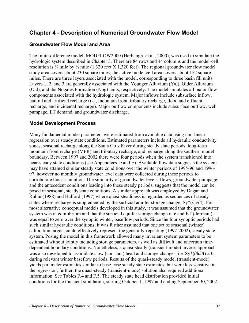
____________________________________________________________________________________________ Chapter 4 – Description of Numerical Groundwater Flow Model 32
Chapter 4 - Description of Numerical Groundwater Flow Model Groundwater Flow Model and Area The finite-difference model, MODFLOW2000 (Harbaugh, et al., 2000), was used to simulate the hydrologic system described in Chapter 3. There are 84 rows and 44 columns and the model-cell resolution is ¼ mile by ¼ mile (1,320 feet X 1,320 feet). The regional groundwater flow model study area covers about 230 square miles; the active model cell area covers about 152 square miles. There are three layers associated with the model, corresponding to three basin fill units. Layers 1, 2, and 3 are generally associated with the Younger Alluvium (Yal), Older Alluvium (Oal), and the Nogales Formation (Nog) units, respectively. The model simulates all major flow components associated with the hydrologic system. Major inflows include subsurface inflow, natural and artificial recharge (i.e., mountain front, tributary recharge, flood and effluent recharge, and incidental recharge). Major outflow components include subsurface outflow, well pumpage, ET demand, and groundwater discharge. Model Development Process Many fundamental model parameters were estimated from available data using non-linear regression over steady state conditions. Estimated parameters include all hydraulic conductivity zones, seasonal recharge along the Santa Cruz River during steady state periods, long-term mountain front recharge (MFR) and tributary recharge, and recharge along the southern model boundary. Between 1997 and 2002 there were four periods when the system transitioned into near-steady state conditions (see Appendices D and E). Available flow data suggests the system may have attained similar steady state conditions over the winter periods of 1995-96 and 1996-97, however no monthly groundwater level data were collected during these periods to corroborate this assumption. The similarity of groundwater levels, flows, groundwater pumpage, and the antecedent conditions leading into these steady periods, suggests that the model can be posed in seasonal, steady state conditions. A similar approach was employed by Dagan and Rubin (1988) and Halford (1997) where quasi-steadiness is regarded as sequences of steady states where recharge is supplemented by the surficial aquifer storage change, Sy*(∂h/∂t). For most alternative conceptual models developed in this study, it was assumed that the groundwater system was in equilibrium and that the surficial aquifer storage change rate and ET (dormant) was equal to zero over the synoptic winter, baseflow periods. Since the four synoptic periods had such similar hydraulic conditions, it was further assumed that one set of seasonal (winter) calibration targets could effectively represent the generally-repeating (1997-2002), steady state system. Posing the model in this framework allowed many invariant system parameters to be estimated without jointly including storage parameters, as well as difficult and uncertain time-dependent boundary conditions. Nonetheless, a quasi-steady (transient-mode) inverse approach was also developed to assimilate slow (constant) head and storage changes, i.e. Sy*(∂h/∂t) ≠ 0, during relevant winter baseflow periods. Results of the quasi-steady model (transient-mode) yields parameter estimates similar to base-case steady state estimates, but were less sensitive in the regression; further, the quasi-steady (transient-mode) solution also required additional information. See Tables F.4 and F.5. The steady state head distribution provided initial conditions for the transient simulation, starting October 1, 1997 and ending September 30, 2002.

____________________________________________________________________________________________ Chapter 4 – Description of Numerical Groundwater Flow Model 33
The model was also simulated from October 1, 1949 through September 30, 1959 to examine model function over pre-effluent conditions. An important objective of this project was to estimate model parameters representing regional-scale properties and tendencies of the system (long-term, quasi-stationary 1982-2002). Over the transient period, storage parameters and time-dependent boundaries, including seasonal evapotranspiration and streamflow-routing parameters were calibrated over a fairly wide range of conditions, including periods of storage gain, loss and near steady flow. However, consecutively-measured groundwater levels are dependent on previous conditions, or are autocorrelated. Most inner valley groundwater levels measured at near-monthly intervals between 1997 and 2005 show considerable autocorrelation. The resulting correlograms also show a gradual decline in autocorrelation followed by cyclical trends, inferring that random processes are superimposed on periodic processes (Haan, 1977). By definition, autocorrelated observations such as successive transient groundwater levels aren’t random and contain less information (and are less sensitive, see Table F.5) about invariant properties such as hydraulic conductivity than random samples (Haan, 1977). Because autocorrelated data adds little information about invariant system parameters, it was assumed that the possible loss of information that might occur by not estimating time-dependant parameters was worth sacrificing for the significant benefits gained by allowing for the efficient evaluation of alternative conceptual models; these conclusions are consistent with the findings of Dagan and Rubin (1988), and Carrera and Neuman (1986c). Additional complications of simultaneously estimating both invariant and time-dependent parameters and storage are discussed by Halford (1997; 1998). There are also compounding uncertainties associated with important transient boundary conditions including the stream-aquifer boundary function, streambed elevation changes over time, and ET boundary conditions that are either less problematic or non-existent during steady state conditions. Therefore, the time-invariant parameters including all k-zones, and long-term MFR and tributary recharge were estimated over steady state (or quasi-steady) conditions, and then were kept constant while time-dependent boundary conditions (and storage) were calibrated during the transient simulation period. Most of the time spent on this project was directed towards exploring alternative conceptual models and examining parameter reliability. Examining alternative conceptual models is the most important aspect of groundwater modeling and is facilitated by inverse modeling (Poeter and Hill, 1997; Bredehoeft, 2003; Carrera et al., 2005; and Neuman and Wierenga, 2003). From a practical standpoint, examining numerous alternatives conceptual models was made possible only by posing the inverse models in a steady state (or quasi-steady) framework, where reliable observation data can support the calibration. For this investigation, alternative conceptual models consisted of exploring wide ranges of model properties and features. Some of the alternative conceptual models examined include:
• Alternative K-zone structures. The final K-zones shown in Figures 4.5, 4.6 and 4.7 represent near-optimal K-zone structure (based on available data). Examining K-zone structure was extremely important in understanding and defining the parameters in the system. For example, the inner valley Oal, i.e. K24 and K10, could not be modeled as a single K-zone without increasing model error by over 40%. Further, the inner valley Yal, i.e. K2 and K6, could not be modeled as a single K-zone without increasing model error

____________________________________________________________________________________________ Chapter 4 – Description of Numerical Groundwater Flow Model 34
by about 80%. However, the Amado and Tubac Sub-areas (Oal) could be combined to form a single Oal K-zone (Koal_North) without losing model accuracy; combining these K-zones reduced functional dependence between Koal’s and tributary recharge, which consequently improved parameter reliability (Nelson, 2003) for all viable models explored during the model development process
• Alternative basin-fill geometries associated with the Oal and Yal units • Alternative Yal lateral extents including expanding and retracting Yal active boundary • Alternative scaled-models, i.e. truncated southern and northern boundary extents • Alterative boundary conditions associated with the southern and northern model
boundaries; for example imposing direct recharge instead of head-dependent boundaries (HDB); applying alternative head elevations (GHB & CHB) and/or conductance’s (GHB) associated with head-dependent boundaries
• Alterative boundary conditions associated with stream-aquifer boundary (Prudic, 1989) o Examining Manning’s’ N option of stream-aquifer boundary (i.e., calibrating
roughness coefficient, etc.) o Examining alternative streambed elevations, streambed thicknesses, stages (when
Manning’s N option not used), streambed gradients o Alternative clogging layer properties and reach extents o Examining direct recharge between Tubac and Elephant Head Bridge, i.e. losing
reach; this was ultimately replaced with the stream-aquifer boundary • Alternative MFR and tributary recharge distributions • Alternative Kx, Ky and Kz ratios; Kz: Ky ratio set to 1:1 due to Ky insensitivity • Examined hypothetical aquitards; ruled out regional-scale aquitards(s) within inner-
valley due to larger-model errors (at least based on available data); Kxy:Kz ratio was ultimately set to 10:1 for all K zones
• Alternative weighting-schemes associated with heads, flows and a-priori data • Developing alternative models with, and without, a-priori data. For this project prior
information was used sparingly as advocated by USGS (Hill, 1998) and Menke (1996) • Alternative incidental recharge rates; including incidental recharge as a variable in the
regression • Alternative (seasonal) steady state well pumping and distribution rates • Developing alternative pre-development steady state models, circa 1880 • Alternative land-surface elevations, i.e. there was inherently land-surface elevation
errors associated with the DEM model; moreover, the streambed elevations change over time
• Quasi-steady parameter estimation in the transient-mode where recharge is supplemented by a constant surficial aquifer storage change, Sy*(∂h/∂t)
• “Warm-up” transient simulations (See section, Transient State Assumptions) • Alternative ET parameters including maximum ET rate and extinction depths • Alternative Sy and Ss parameters
Alternative conceptual models were tested for viability and reliability using the criteria defined by the USGS including 1) better fit; 2) weighted residuals that are randomly distributed, and 3) realistic parameters (Hill, 1998). In general a parsimonious - or simplified - approach was taken regarding the model parameterization as advocated by the USGS (Hill, 1998). No single “best”

____________________________________________________________________________________________ Chapter 4 – Description of Numerical Groundwater Flow Model 35
conceptual model was identified with absolute certainty. Fortunately, most viable models tend to share similar optimal parameter values and reliability information for those parameters estimated within the inner Santa Cruz River Valley. The “final” conceptual model presented herein balances model accuracy, with parameter uncertainty. To convey parameter reliability and parameter sensitivity, statistics associated with the estimated parameters are presented in Appendix F. In this report, the measure used for examining parameter sensitivity is based on the inverse model statistics, thus replacing the traditional sensitivity analysis because the latter does not generally account for parameter interdependencies, etc. (see Hill, 1994; Cooley and Naff, 1990; Poeter and Hill, 1997; Carrera and Neuman, 1986a and 1986c; Carrera et al., 2005). Some time-dependent boundary conditions and storage parameters were not estimated using inverse modeling techniques; nonetheless, qualitative discussions about trial-and-error calibrated boundary conditions and parameters are provided in relevant sections. The model was primarily calibrated between 1997 and 2002 because of high quality data collected over this period including hydraulic head, flow, and pumpage data. The lack of reliable data prior to the mid-1990’s would have made a calibration prior to this period problematic, wrought with many difficult assumptions. Some of the data deficiencies include: No well pumping records prior to the mid-1980’s; no observed flow data prior to the mid-1990’s; effectively no observed monthly (or even seasonal) head data between the late 1950’s and fall of 1997; effectively no observed groundwater level data outside the inner valley system prior to 1982. Nonetheless, the period between 1997 and 2002 covers a wide range of hydrologic conditions including flood recharge (both moderate and extreme events), drought periods, as well as four periods when the system was in near-steady state conditions. Concentrating the model calibration over periods where reliable hydraulic head, flow, and pumping data exists enabled most model parameters to be estimated with a relatively high degree of certainty in the Santa Cruz River Valley. Despite the aforementioned historical data limitations, the model was also simulated from October 1949 through September 1959 to examine transient model function over pre-effluent conditions. This was a relatively dry period with no effluent recharge, significant groundwater pumpage, and river channelization. Flow data collected outside the model area infers that this period also experienced two extreme monsoon recharge periods in 1954 and 1955. Despite the data gaps, the 1950’s simulation provided additional insight about the model, its capabilities, and stress period requirements. An alternative pre-development (representative of conditions prior to 1880) steady state simulation was also developed for winter, baseflow conditions. As with the 1949-59 transient simulation, there were some very difficult modeling and data assumptions associated with the pre-development conditions. Nonetheless, it was instructive to compare parameter estimates (and parameter reliability information) for pre-development and recent conditions, and to examine simulated water budgets without groundwater pumpage. Model Units, Model Code, Pre-and Post Processors Model units for length and time were feet and days, respectively. The model code selected to simulate groundwater flow was the modular three-dimensional finite difference groundwater flow model, MODFLOW 2000, developed by the U.S. Geological Survey (McDonald and

____________________________________________________________________________________________ Chapter 4 – Description of Numerical Groundwater Flow Model 36
Harbaugh, 1988; Harbaugh, et al., 2000). MODFLOW 2000 was selected for use in this project because:
• MODFLOW 2000’s modular format allows specific hydrologic features and stress to be simulated
• The code enables the different units to be interconnected • Complete documentation • The Code is widely used and is accepted as a valid model for simulating groundwater
flow For this project, the pre-and-post-processor Visual MODFLOW™, Version 3.1 (Visual MODFLOW, 2003) was used to create the raw model datasets for MODFLOW 2000. Visual MODFLOW also provides a direct link to the parameter estimation program, WinPEST™ (WinPEST, 2003), which was used extensively in this investigation. The Governing Groundwater Flow Equations The governing flow equation that describes the movement of constant density groundwater through porous media is ∂ (Kxx ∂h) + ∂ (Kyy ∂h) + ∂ (Kzz ∂h) – W = Ss ∂h Equation 4.1 ∂x ∂x ∂y ∂y ∂z ∂z ∂t where Kxx, Kyy, and Kzz are values of hydraulic conductivity along the x, y and z coordinate axes (Lt-1), h is the potentiometric head (L), W is a volumetric flux per unit volume (i.e. sources and/or sinks), Ss is the specific storage of the porous material (L-1), and t is time (t) (McDonald and Harbaugh, 1988). The solution of 4.1 gives h(x,y,z,t) when the derivatives of h with respect to time and space are substituted into equation 1, and the boundary and initial (transient-only) conditions are satisfied (McDonald, Harbaugh, 1988). The transient groundwater flow system is fully described by equation 4.1, where the energy of subsurface flow and the volume of water in storage are used to calculate the direction and flow rate associated with the movement of groundwater. When groundwater flow rates and directions are constant over space, ∂h/∂t = 0, then steady state conditions exist and the right side of equation 4.1 is equal to zero. Analytical solutions for the continuous partial differential equation 4.1 are only available for simple groundwater flow systems. However, practical solutions for more complicated hydrologic systems can be approximated by applying discrete representations over space and time. One discrete approach of approximating equation 4.1 is the finite-difference method used by MODFLOW. The finite difference method enables the hydrologic system to be represented by individual model cells. Groundwater flow to and from model cells is represented by a system of simultaneous linear algebraic difference equations in which the hydraulic head, h, is solved for every active model cell, to within a specified user-defined tolerance. MODFLOW has been updated several times since its inception in the 1980s, and for this project MODFLOW 2000 was used. See McDonald and Harbaugh (1988) and Harbaugh et al., (2000).

____________________________________________________________________________________________ Chapter 4 – Description of Numerical Groundwater Flow Model 37
Model Features MODFLOW consists of different subroutines (i.e., modules) that simulate the groundwater flow system. The modules used in this study include the Basic (BAS), Layer Property Flow (LPF – MODFLOW 2000), Discretization (DIS), Well (WEL), Recharge (RCH), Evapotranspiration (ET), General Head Boundary (GHB), and Streamflow Routing (STRM) packages. For this particular investigation, the strongly implicit procedure (SIP) package was used to solve the linear, groundwater flow equations. For details on the different modules see section below. BASIC (BAS) Package The BAS package defines the physical geometry of the model by assigning cell rows, columns, and layers. Simulation time and model length units are also associated with the BAS package. Model cells are designated either as active or inactive in the BAS package. Starting groundwater levels for each active cell are assigned in the BAS package. Constant head boundary (CHB) cells are assigned through the Ibound array within the BAS packages. In this model, CHB cells are assigned along portions of the inflow and outflow boundary. Layer Property Flow (LPF) and Discretization (Dis) Package The LPF and DIS packages calculate the flow of water between active model cells under steady state and transient conditions. To determine flow between model cells, the LPF and DIS packages contain information about the geologic structure and the cell-centered hydraulic parameters of the model. The harmonic mean defines the potential rate of flow through adjacent horizontal and vertical cells as defined by the hydraulic conductivity and cross-sectional area of the cells. The hydraulic parameters are cell-specific and include hydraulic conductivity and storage terms. Layer 1 is defined as an unconfined aquifer (i.e., LAYCON1). Layers 2 and 3 are convertible confined/unconfined aquifers assigned with LAYCON3. For features associated with the LPF and DIS package, see McDonald and Harbaugh (1988) and Harbaugh, et al., (2000). The rewetting option was not used during the 1997-2002 simulations (including steady state inverse model solutions) because the model was specifically designed to prevent hydraulic heads from dropping below unit boundary elevations, primarily in the Yal unit where most groundwater level fluctuations occur. When significant changes-in-storage are simulated, especially over relatively short time intervals, the abrupt introduction of water to a previously “dry” cell can lead to solution difficulties, as well as water budget errors. The rewetting of dry cells, which is a well known problem associated with MODFLOW, became a serious difficulty in a previous modeling investigation of the Santa Cruz AMA (McSparran, 1998). Because of these concerns, efforts were made to reduce the potential for encountering dry cells before they became problematic. The rewetting option was, however, activated for the 1949-1959 transient calibration and simulation, because the initial heads during this period were lower than during the 1997-2002 simulation period. The lower heads yielded three dry cells in Yal aquifer during the 1949-59 simulations in model cells (row/column): 25/16, 68/27 and 78/35. During the 1949-59 simulation, the rewetting option was activated to allow for rewetting of these cells in response to the flood recharge. Some convergence difficulties were encountered due to the rewetting of these previously dry cells. To counter instability, the SIP closure criterion was loosened from

____________________________________________________________________________________________ Chapter 4 – Description of Numerical Groundwater Flow Model 38
0.01 to 0.1, thus allowing a solution. Despite changes in SIP closure, the resulting mass balance errors were generally less than 0.05 (for details see Reilly and Harbaugh, 2004). To reduce the risk of encountering dry cells some peripheral Yal cells that had minimal saturated thickness, were truncated. That is, model cells in areas susceptible to significant head fluctuation where the Yal thins out – thus vulnerable to dewatering - were de-activated. Because the areal extent of Yal cells prone to dewatering is relatively small, the model error associated with the truncation is assumed to be minimal. In fact when cells 25/16, 68/27 and 78/35 (i.e., the cells that went dry during the 1949-59 simulation when groundwater levels were very low, but were active over the recent periods) were de-activated, the resulting inverse model solution was nearly identical to the base-case solution. When the Yal boundary was expanded (widened) by activating more Yal lateral model cells with respect to the base-case Yal boundary, the solution was also similar to the base-case model. The consequential benefits of preventing model cell dewatering are assumed to greatly outweigh the potential difficulties associated with re-wetting dry cells. With the exception of the Rio Rico Bridge well site (near the southeast model boundary), and the northern portion of the model near Amado, groundwater level fluctuations throughout the model domain are relatively small. It should be noted that the drying and rewetting of model cells also has a detrimental effect on the MODFLOW parameter estimation process. If a model cell goes dry then the response of the model is no longer continuous with respect to the adjustable parameters. Interruptions between model cells and adjustable parameters prohibits calculation of Jacobian and covariance matrices (see WinPEST, 2003), and thus undermines efforts to rigorously examine parameter reliability, which is a major objective of this investigation. In addition, designing the model to generally result in good head clearance above respective unit boundaries reduces the potential for problems associated with LAYCON 3 setting, and the subsequent conversion between Ss and Sy, if/when a cell goes dry in an unconfined aquifer. Also see section below on Specific Yield and Specific Storage. WELL (WEL) Package The WEL package is used to simulate groundwater withdrawals from wells. In this model, the well package was used to simulate non-exempt pumpage from agriculture, industrial, municipal, and domestic demands over steady state and transient conditions. Well Pumpage: Steady State Conditions The location and rate of non-exempt well pumpage imposed to the steady state simulation was based on recorded pumpage listed in the ROGR database (ADWR_ROGR, 2004). See Figure 4.4 for locations and rates of average well pumpage recorded during the 1997-2002 winter periods. Well pumpage was imposed at rates representative of typical, non-summer conditions. Based on a survey of agricultural water use in the Santa Cruz AMA, it is estimated that about 30 to 40% of the total agricultural water demand occurs over non-summer periods for the irrigation of crops such as wheat, winter mix (i.e., combinations of barley, oats, and rye) and permanent pasture (Nelson, 1998). Estimates/records for municipal, domestic, and industrial groundwater demand during non-summer periods is about 50% of the annual demand (ADWR_RORG, 2004; personnel communication with Don Baker, 2004; and Denny Scanlan, 2004, utility managers for Rio Rico and Tubac, respectively). Therefore, the non-summer pumpage (i.e., between October

____________________________________________________________________________________________ Chapter 4 – Description of Numerical Groundwater Flow Model 39
1st and April 30th) represents about 40% of the annual groundwater pumping demand for the agricultural, industrial, municipal and domestic sectors. The total groundwater pumpage recorded in the model area in 1999 and 2000 averaged about 15,800 AF/YR, or about 22 cfs; this rate is consistent with pumpage recorded between 1995 and 2002. If 40%, or 6,320 AF, was extracted from the groundwater system between October 1st and April 30th (seasonalized volume over 212 days), then the pumping rate over this period is equal to an annualized discharge rate of about 10,800 AF/YR, or about 15 cfs (base-case rate). This assumption implies that the summer demand volume was about 9,480 AF (seasonalized volume over 153 days between May 1 through September 30), resulting in an annualized summer well groundwater discharge rate of about 22,600 AF/YR, or about 31 cfs. In other words the groundwater pumping rate in summer is about twice that of winter pumping rates. Although there is good control over annual groundwater pumping rates (ADWR_ROGR, 2004) there remains some uncertainty regarding the exact seasonal pumping rate; furthermore, there are also slightly different pumping rates imposed over the four quasi-steady-state synoptic periods. Because of this, some alternative, seasonal (non-summer) pumping rates were examined. Alternative models simulating quasi-steady pumpage at rates between 30%-45% of annual demand produced similar solutions with similar parameter-estimation statistics; thus the model was, to an extent, insensitive when imposing seasonal quasi-steady pumpage rates between 8,200 and 12,200 AF/YR. However, the most accurate model solutions simulated about 10,800 AF/YR of seasonal, quasi-steady pumpage. Thus, the final steady state base-case pumping rate was imposed at an annualized rate of approximately 10,800 AF/YR, and includes about 300 AF/YR (annualized) of exempt domestic pumpage. Well (WEL) Pumpage: Transient State Conditions Locations and rates of non-exempt pumpage imposed over the transient simulation were based on the ROGR database (ADWR, 2003). Pumpage rates for non-exempt wells were simulated at two seasonalized rates: 1) summer periods between May 1st and September 30th (153 days), and 2) non-summer periods between October 1st and April 30th (212 days). Summer demand rate is assumed to equal about 60% of the total annualized volume. In the model, the two generalized seasonal rates were further sub-divided into the five individual stress-period rates (for stress-period definition, see section titled, “Assumptions Associated with Transient State Solution”). Most groundwater pumpage in the Santa Cruz AMA originates from non-exempt wells. Non-exempt wells have pumping capacities greater than 35 gallons-per-minute, and comprise about 95% of all current pumping demand in the Santa Cruz AMA. Because all non-exempt wells are required to report their discharge, the annualized discharge volumes are assumed to be accurate and reliable. The accuracy associated with non-exempt pumping is important in that it provides good control on pumping discharge rates, and act to reduce parameter uncertainty in the regression. Groundwater withdrawal from exempt wells currently constitutes a relatively small portion of the overall pumpage in the model area (probably less than 5%). As indicated in the Santa Cruz AMA Third Management Plan (ADWR_TMP, 2000), exempt wells currently have relatively little impact on water tables. Domestic well pumpage was estimated at about 300

____________________________________________________________________________________________ Chapter 4 – Description of Numerical Groundwater Flow Model 40
AF/YR. Most of the domestic demand is concentrated in the Tumacacori, Carmen, Tubac, and Amado areas. Recharge (RCH) Recharge was applied to the uppermost active model layer. Recharge was used to simulate long-term tributary and mountain front recharge, incidental recharge, recharge along the Santa Cruz River over steady state periods (during model development), and inflow boundary-condition recharge. At various times during the model development process, all recharge components, along with all hydraulic conductivity zones, were estimated as independent parameters in the non-linear regression. As more information about parameter reliability became available, some parameters were either combined, fixed, tied as ratios, or converted to head-dependant boundaries (for more details on this aspect of the calibration see sections below). Infiltration of precipitation and streamflow along major tributaries and MFR areas are important natural inflow components of the hydrologic system. For model conceptualization purposes, MFR and tributary recharge are assumed to contribute recharge at constant rates over steady state and transient periods. Although peripheral MFR and tributary recharge obviously vary over time, applying recharge at long-term uniform rates greatly simplifies the model, and focuses the model calibration towards the fundamental relation between hydraulic conductivity and recharge (note that periodic recharge will be accounted in the stream boundary associated with the Santa Cruz River and major confluences). This assumption requires that uniform steady state recharge rates reflect long-term average recharge rates. Reilly and Pollock (1996), Maddock and Vionnet (1998), Dickinson et al. (2004) and Halford (1998) provide discussion regarding steady state recharge, and the processes related to the attenuation of cyclical recharge over space and time. Estimated rates of long-term MFR and tributary recharge, as determined by the inverse model solution, were then applied as specified fluxes during the 1997-2002 transient simulation. Mountain Front Recharge (MFR) A total of five MFR zones were assigned in the model. MFR cells are distributed along the flanks of mountain front areas. Variations to the areal MFR rate and distribution were evaluated during the model development process for accuracy and reliability. In general, MFR zones where more precipitation and recharge are assumed to occur, such as along the windward side of the high-elevation Santa Rita Mountains, were assigned higher starting MFR rates in the parameter estimation process, and led to more accurate and less biased solutions. The five individual MFR zones were independently un-resolvable due to either low parameter sensitivity or extreme parameter correlation among the recharge and the hydraulic conductivity zones. As a result, the five individual zones were combined to form two independent MFR zones to increase sensitivity in the regression (Zones 1 and 2). Although combining all MFR zones into two independent parameters increased the parameter sensitivity, combining the parameters did not reduce the extreme parameter correlation between MFR and hydraulic conductivity parameter (i.e., Nogales Formation, Knog). Different starting values of MFR yielded different MFR rates in the regression, thus inferring extreme correlation. The final composite MFR rate of 1,900 acre-feet/year is less than conceptual estimates, but provides a more accurate solution,

____________________________________________________________________________________________ Chapter 4 – Description of Numerical Groundwater Flow Model 41
based on available data. It should be noted that the model does not explicitly differentiate mountain block recharge from direct infiltration recharge. See Table 4.1 and Figure 4.1. Table 4.1 Estimated Mountain Front Recharge
LOCATION PARAMETER ZONE Long-term Estimated MFR Rate (AF/YR)
Upper Sopori Wash/Diablo Mountain 1a 140 Tumacacori and Atascosa Mountains 1b 220 Upper Josephine Canyon 1c 40 San Cayetano Mountains 1d 40 Santa Rita Mountains (western, southern windward slope)
2 1,460
TOTAL 1,900 Tributary Recharge Natural tributary recharge was estimated as an independent parameter in all conceptual models. As with MFR, estimated tributary recharge was applied at uniform rates over the transient solution based on the long-term steady state solution. Conceptual estimates for tributary recharge are approximately 6,600 acre-feet/year (Aldridge and Brown, 1971; Halpenny and Halpenny, 1989). Tributary recharge is represented by imposing recharge cells along major tributaries near the inner Santa Cruz River Valley. A total of thirteen major tributaries were included in the regression. It was not possible to independently estimate tributary recharge for each tributary due to parameter insensitivity. As a result, all thirteen tributaries were tied together in the regression to increase parameter sensitivity and improve reliability. It’s been assumed that coarse-grain sediments associated with major tributaries – especially near the Santa Cruz River confluences - provide efficient hydraulic mechanisms for recharge, similar to the inner Santa Cruz River Valley. Outside major tributary areas where the Oal unit is generally overlain by terrace and pediment deposits (Drewes, 1972b), infiltration is assumed to be insignificant. An alternative conceptual model was developed to examine how uniform tributary recharge compares with cyclic tributary recharge. The alternative, cyclic transient model assumes that two-thirds of all tributary inflow occurs over flood-dominated stress periods. The cyclic recharge model produced results that were comparable to the base-case results, which is consistent with Reilly and Pollock (1996). However, it must be noted that these results may not apply to extended long-term cycles/trends, for example periods that extend over a 10 consecutive-year dry or wet cycle. See Table 4.2 and Figure 4.1.

____________________________________________________________________________________________ Chapter 4 – Description of Numerical Groundwater Flow Model 42
Table 4.2 Conceptual and Estimated Tributary Recharge LOCATION CONCEPTUAL
(AF/YR) LONG-TERM ESTIMATED
MFR RATE (AF/YR) Lower Sonoita Creek 800 640 Agua Fria Canyon 700 640 Peck Canyon 700 640 Un-named Rio Rico 500 N/A Josephine Canyon 500 750 1Rock Corral Canyon 500 430 1Aliso Canyon 500 430 Mavis Canyon 300 640 Tubac Creek 300 430 Cottonwood Canyon 200 640 Diablo Canyon 200 320 Montosa Canyon 200 640
600 860 2Upper Sopori Wash Lower Sopori Wash 500 860 Lower Agua Caliente Canyon 100 430 TOTAL 6,600 8,350 1Not included in Aldridge and Brown (1971); adding these tributaries significantly improved the reliability of recharge estimates. 2Upper Sopori Wash based on Halpenny (1989)

____________________________________________________________________________________________ Chapter 4 – Description of Numerical Groundwater Flow Model 43
Figure 4.1 Distribution of Mountain Front and Tributary Recharge

____________________________________________________________________________________________ Chapter 4 – Description of Numerical Groundwater Flow Model 44
Recharge along the Santa Cruz River Recharge along the Santa Cruz River was estimated between Tubac and Elephant Head (losing reach) during steady state, or quasi-steady conditions. The inverse model provided optimal recharge rates, as well as information about parameter reliability. Optimal recharge rates were then converted to head-dependent boundaries. Interaction between surface water and groundwater is simulated by MODFLOW via the head-dependent stream-routing package boundary (Prudic, 1989). Numerous features of the SR boundary were examined during the model development process including vertical streambed conductivity (stream Kz), streambed thickness (stream M), streambed width (stream W), and stream stage (Hstrm) including the option of applying the Manning’s N coefficient, alternative streambed elevations, and alternative streambed gradients. A complete description of these properties are described in Appendix C. For location of streamflow boundary cells, see Figure 4.2. Incidental Agriculture Recharge Based on previous studies and surveys described in Chapter 3, the incidental agriculture rate was fixed at 25% of the agriculture demand rate for steady state and transient conditions. Agricultural-related pumpage in the model area typically represents about 60% of the total groundwater pumping demand, or about 10,000 AF/YR (13.8 cfs). Summer (152 days) and non-summer (212 days) agricultural demands account for about 60% and 40% of the annualized pumpage, respectively. Therefore, if the incidental recharge rate is 25%, the average annual incidental recharge rate is about 2,500 AF/YR. Seasonal incidental recharge rates applied over summer and non-summer periods are about 5.0 cfs and 2.5 cfs, respectively. Thus, the annualized, non-summer incidental recharge rate averages about 1,700 AF/YR. Incidental agriculture recharge was imposed at a rate of 25% groundwater pumpage to model cells located on, or near, the representative field location in the steady state and transient simulations. No time-lag was imposed to incidental agriculture recharge because of the highly dispersive nature of the aquifers, and the shallow depth-to-waters. As with the assigned pumping demand, it is acknowledged that the actual rate of incidental recharge varies over space and time and depends on many different factors. However, the incidental recharge rate applied in this study represents the most probable, regional-scaled-averaged rate given the available information to date. During the model development process, incidental recharge was estimated as an independent parameter. The inversion statistics show extreme parameter correlation between tributary recharge and incidental agricultural recharge; this relation is not surprising considering their close spatial locations, and the high transmissivity of the inner valley aquifers. Because of this, incidental recharge was fixed as a percentage of recorded agriculture pumpage. Omitting incidental agriculture recharge as an independent variable enabled other system parameters to be independently evaluated in the regression with greater certainty. Evapotranspiration (ET) The ET package simulates groundwater discharge from the saturated zone based on the estimated riparian demand located primarily within the inner Santa Cruz River Valley. ET demand is represented by a head-dependent boundary based on a linear-demand function. See McDonald

____________________________________________________________________________________________ Chapter 4 – Description of Numerical Groundwater Flow Model 45
and Harbaugh (1988). GIS information was used to create a composite ET demand for each applicable model ET cell. As a result each raw, composite ET cell has a different associated ET demand rate. Because of the high resolution associated with the ET delineation (Masek, 1996), some composite ET cells may include all seven vegetation class-rates, listed in Table 3.2. The land elevation reference was based on DEM elevation models. To simplify the calibration procedure, composite ET demand was aggregated into eleven distinct maximum ET rates (zones), which were then distributed over the five stress periods –per-year, as a function of season. A generalized ET extinction depth of 35 feet was assigned to the ET boundary (personal communication with Julie Stromberg, 2006). Infrared photographs reveal an increase in vegetation along the river between 1993 and 2004 due to periodic yet intensive recharge during 1993/94, 1998 and 2000/01 winter periods, which promoted shallow water tables. Accordingly, some adjustments were made to ET parameters during the transient calibration to accommodate recent ET proliferation. Alternative conceptual models were developed to examine different ET parameters including different extinction depths and maximum ET rates. There remains uncertainty about the ET targets rates, i.e. saturated verses the unsaturated ET targets rates (Scott, et al., 2000), as well as surface elevations references which change over time. It should be noted that this model does not simulate ET in the unsaturated zone. This problem is further compounded due to the interdependence between the ET and stream-aquifer boundary assigned over summer periods. An important benefit of constraining the steady state solution to winter (dormant) periods is that ET rate can be neglected in the parameter estimation process, consequently eliminating an uncertainty that would otherwise need to be accounted for in the model solution. Model Geometry Associated with the Basin-Fill Units The structure and geometry of the NOG and Oal geologic units were based on interpretations of Gettings and Houser (1997) and HydroGEOPHYSICS (2001). Carruth (1996) provides structural descriptions for the Yal unit. These investigations used geophysical techniques including gravity, aeromagnetic, acoustic soundings and existing well log data for the interpretation of the basin-fill geometry. Because of the uncertainty associated with the basin-fill units, alternative conceptual models were developed to further examine the geologic structure associated with the Oal and Yal units. Alternative conceptual models based on different geometrical configurations of Oal and Yal include:
• Increasing and decreasing the thickness of the Oal unit by approximately plus and minus 25%, respectively, in the: 1) Rio Rico, 2) Tubac and 3) Amado Sub-areas;
• Increasing and decreasing the thickness of the Oal unit between the Rio Rico and Tubac Sub-areas by approximately plus and minus 25%, respectively; this area represents a transition zone contrasting two distinctive permeable areas in the Oal unit aquifer;
• Increasing and decreasing the thickness of the entire Yal unit by plus and minus 20 feet • Extending and retracting the areal extent of Yal unit, i.e., adding and removing Yal cells
Although the basin geometry affected parameter estimates, most alternative geologic conceptualizations had relatively little effect on the overall estimation of transmissivity, inferring near-unique transmissivities. For example, when the Yal unit thickness was globally decreased by 20 feet, the estimated Yal hydraulic conductivity in the Rio Rico Sub-area changed from
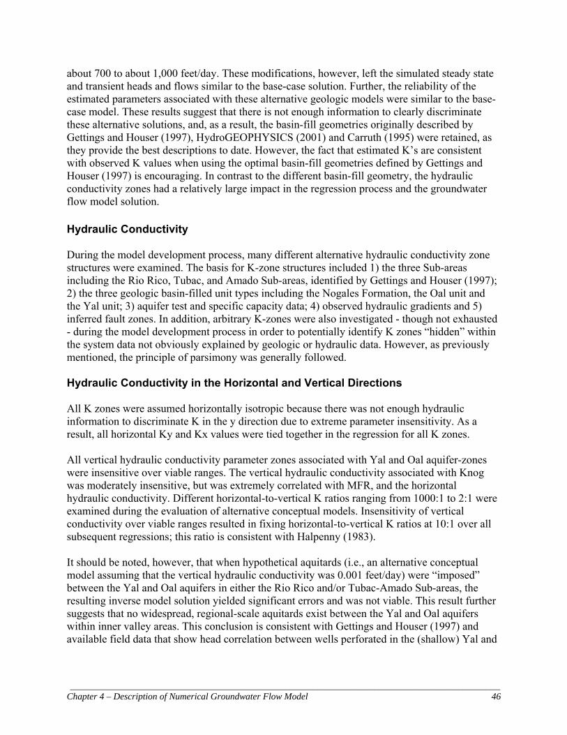
____________________________________________________________________________________________ Chapter 4 – Description of Numerical Groundwater Flow Model 46
about 700 to about 1,000 feet/day. These modifications, however, left the simulated steady state and transient heads and flows similar to the base-case solution. Further, the reliability of the estimated parameters associated with these alternative geologic models were similar to the base-case model. These results suggest that there is not enough information to clearly discriminate these alternative solutions, and, as a result, the basin-fill geometries originally described by Gettings and Houser (1997), HydroGEOPHYSICS (2001) and Carruth (1995) were retained, as they provide the best descriptions to date. However, the fact that estimated K’s are consistent with observed K values when using the optimal basin-fill geometries defined by Gettings and Houser (1997) is encouraging. In contrast to the different basin-fill geometry, the hydraulic conductivity zones had a relatively large impact in the regression process and the groundwater flow model solution. Hydraulic Conductivity During the model development process, many different alternative hydraulic conductivity zone structures were examined. The basis for K-zone structures included 1) the three Sub-areas including the Rio Rico, Tubac, and Amado Sub-areas, identified by Gettings and Houser (1997); 2) the three geologic basin-filled unit types including the Nogales Formation, the Oal unit and the Yal unit; 3) aquifer test and specific capacity data; 4) observed hydraulic gradients and 5) inferred fault zones. In addition, arbitrary K-zones were also investigated - though not exhausted - during the model development process in order to potentially identify K zones “hidden” within the system data not obviously explained by geologic or hydraulic data. However, as previously mentioned, the principle of parsimony was generally followed. Hydraulic Conductivity in the Horizontal and Vertical Directions All K zones were assumed horizontally isotropic because there was not enough hydraulic information to discriminate K in the y direction due to extreme parameter insensitivity. As a result, all horizontal Ky and Kx values were tied together in the regression for all K zones. All vertical hydraulic conductivity parameter zones associated with Yal and Oal aquifer-zones were insensitive over viable ranges. The vertical hydraulic conductivity associated with Knog was moderately insensitive, but was extremely correlated with MFR, and the horizontal hydraulic conductivity. Different horizontal-to-vertical K ratios ranging from 1000:1 to 2:1 were examined during the evaluation of alternative conceptual models. Insensitivity of vertical conductivity over viable ranges resulted in fixing horizontal-to-vertical K ratios at 10:1 over all subsequent regressions; this ratio is consistent with Halpenny (1983). It should be noted, however, that when hypothetical aquitards (i.e., an alternative conceptual model assuming that the vertical hydraulic conductivity was 0.001 feet/day) were “imposed” between the Yal and Oal aquifers in either the Rio Rico and/or Tubac-Amado Sub-areas, the resulting inverse model solution yielded significant errors and was not viable. This result further suggests that no widespread, regional-scale aquitards exist between the Yal and Oal aquifers within inner valley areas. This conclusion is consistent with Gettings and Houser (1997) and available field data that show head correlation between wells perforated in the (shallow) Yal and

____________________________________________________________________________________________ Chapter 4 – Description of Numerical Groundwater Flow Model 47
(deep) Oal aquifers. This result, however, does not rule out the existence of fine-grain material or clay lenses in local areas, or areas outside the inner valley. For more on the determination and distribution of K zones see the section on Parameter Resolution and Model Accuracy Considerations below, and Table 4.3 for the final estimated parameters, and Figures 4.5, 4.6 and 4.7. Southern and Northern Boundary Conditions Head-dependent boundaries were assigned at the southern and northern model boundaries. These head-dependent boundaries represent areas where subsurface flow moves into (primarily from the south), and out-of (predominately to the north) the model area through the three basin-fill unit aquifers, the Yal, Oal, and Nog unit aquifers. Constant head boundaries (CHB) were assigned to areas outside the inner valley. General head boundaries (GHB) were assigned adjacent to inner valley areas, and provide additional flexibility for examining different external conductance’s immediately to outside the active model domain. The external head elevations were assigned one model cell length, or 1,320 feet, outside the model domain. See Figures 4.2, 4.3, 4.4 and Table 4.5 for southern and northern head-dependent boundaries associated with layers 1, 2 and 3, respectively. (Note that most of the east and west lateral model boundaries are no-flow boundaries, but have specified MFR flux imposed, see Figure 4.1). The northern boundary was relatively insensitive to changes in GHB conductance and external head elevation (+/- 5 feet); this result is consistent with the Tucson Model (Mason and Bota, 2006). The assigned GHB conductivity associated with the Yal, Oal, and Nog unit aquifers was 150, 30, and 0.3 feet/day, consistent with available field data; these values are also reasonably consistent with parameter-estimated values. Modification of these values by plus and minus 100%, or replacement with CHB cells, made little difference in the model solution. However, in another alternative model conceptualization, the northern model boundary was relocated four miles south – near the Tubac and Amado Sub-area contact (to row 16, using the appropriate head-reference elevations); the resulting parameter estimation solution was less stable. Results of this “truncated” alternative, suggests that the northern portion of the model area is relatively sensitive and thus important in constraining the regional model solution. Adjacent to the northern model boundary, significant pumpage originates from a mine well located in the Tucson AMA. Hydraulic impacts from this demand and other wells, subsurface flow to the north, as well as recharge along the Santa Cruz River effect groundwater levels along this boundary. Accordingly, the external heads associated with the northern GHB were adjusted to correspond with observed head changes over the transient simulation (1997-2002; and 1949-1959). The model was relatively sensitive to the Yal GHB conductance term assigned at the model’s southern boundary near the NIWTP. Optimally calibrated GHB conductivities assigned at the southern boundary were 400, 5, and 0.3 feet/day for the Yal, Oal, and Nog, respectively. The external head elevation associated with the southern GHB (and adjacent CHB) was moderately sensitive. For the steady state simulation, head elevations assigned to the external GHB and the active CHB were based on groundwater levels measured over the steady state conditions. Groundwater levels associated with the south-eastern GHB boundary were held constant over the steady state and transient simulation, and were assigned a value of 3,450 feet for the Yal, Oal and

____________________________________________________________________________________________ Chapter 4 – Description of Numerical Groundwater Flow Model 48
Nog units. Between 1997 and 2002, groundwater levels immediately south of the NIWTP were effectively regulated by a constant discharge from the Nogales Wash, lining of the upgradient Nogales Wash canal, Potrero Creek, and leaks associated with the NIWTP influent infrastructure. Stable groundwater levels at the southern model boundary since the 1970’s make the external GHB head reference convenient, yet robust. During the 1949-1959 periods, the southern GHB (inner valley) and the southern CHB (west of the inner valley) were adjusted to reflect groundwater level changes during this period. Alternative conceptual models were developed in which the GHB of the Yal and the CHB of the Oal were replaced with direct recharge. These alternative models produced solutions similar to the base-case model, but the parameters were estimated with less reliability. Therefore taking advantage of stable external heads along the southern boundary (i.e. applying head-dependent boundaries instead of direct recharge) significantly increased the reliability of the system parameter estimates. Another alternative conceptual model was developed whereby the southern model boundary was relocated four miles north near the start of the gaining winter reach of the river (from row 84 to row 68, using appropriate head-reference elevations at the new boundary). The resulting parameter estimation solution was less stable, and more susceptible to parameter noise and correlation. Results of this “truncated” alternative, suggest that the southern portion of the Rio Rico Sub-area is sensitive, and important in constraining the model solution.
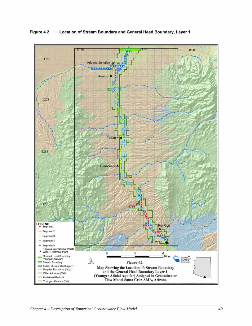
____________________________________________________________________________________________ Chapter 4 – Description of Numerical Groundwater Flow Model 49
Figure 4.2 Location of Stream Boundary and General Head Boundary, Layer 1

____________________________________________________________________________________________ Chapter 4 – Description of Numerical Groundwater Flow Model 50
Figure 4.3 General and Constant Head Boundaries, Layer 2

____________________________________________________________________________________________ Chapter 4 – Description of Numerical Groundwater Flow Model 51
Figure 4.4 Location of Pumpage (in 2000) and Head Boundaries (Layer 3)

____________________________________________________________________________________________ Chapter 4 – Description of Numerical Groundwater Flow Model 52
Steady State Assumptions Between 1997 and 2002 there were four periods when the groundwater system approached steady state conditions. These periods include:1) December 1997 to early February 1998; 2) December 1998 through February 1999; 3) November 1999 into early March 2000 - the primary synoptic period; and 4) December 2001 through February 2002. In the seasonal transition from fall to winter (1997-2002), the regional groundwater flow system generally attained near-equilibrium conditions where observed heads, flows and pumpage were nearly stationary. (Subsequent examination of transient-simulation water budgets show that the groundwater system approaches near-steady conditions over these winter, baseflow periods.) Also note that the high transmissivities associated with narrow inner valley aquifers generally facilitate rapid transition to “instantaneous”, seasonal steady states in the groundwater flow system (Haitjema, 2006). Unlike using long-term or even annually-averaged head and flow targets, which can lead to the over-and-under estimation of global capture in a cyclical system (Maddock and Vionnet, 1998), steady state (or quasi-steady) sequences allow specific, seasonally-based head and flow targets in the regression. The similarity of observed heads, flows and pumpage recorded during winter baseflow periods, suggest that the system can generally be posed a seasonal, steady state condition. In areas outside the inner valley where development is negligible and aquifer transmissivities are generally low, the system reflects time-averaged (long-term) steady states conditions. A quasi-steady, inverse approach was also developed to assimilate slow, constant head changes over time, i.e. Sy*(∂h/∂t) ≠ 0, during relevant winter baseflow periods. Examination of groundwater level data (1997-2002) shows that during certain, winter baseflow periods, areas including Rio Rico (south) and Amado may have been losing small volumes of storage over time. The quasi-steady calibration strategy provided similar results to the true steady state solution except that the system recharge was, generally, supplemented by surficial aquifer storage change. It should be noted that applying the quasi-steady approach required additional assumptions about initial conditions, and storage parameters. See Appendix F.
Schwalen and Shaw (1957) suggest that pre-development groundwater levels were not more than 5 to 6 feet higher than heads recorded in 1940. Based on this assumption, the pre-development (representative of conditions prior to 1880) steady state groundwater levels in the inner valley are assumed to be similar to groundwater level conditions observed in 2000, which were about 5 feet higher than those observed in 1940. See Table D.6. Although 1940 groundwater level data isn’t available for areas outside the inner valley, the 2000 groundwater level observations are assumed to be representative of pre-development conditions in peripheral areas; this remains a difficult assumption. Observation Data and the Non-Linear Regression Inverse models were developed to examine alternative conceptual models including the spatial distribution of all hydraulic conductivity zones, long-term mountain front and tributary recharge, quasi-steady state (seasonal) recharge along the Santa Cruz River, and boundary recharge. The inverse model solutions were constrained by synoptic head data collected over the quasi-steady state period between January and March 2000. A total of 99 groundwater levels were used as hydraulic head calibration targets, and most of the head targets used in the regression were measured between January and March 2000. A number of head targets measured outside the synoptic-period were also included in the regression. In addition, some target heads were

____________________________________________________________________________________________ Chapter 4 – Description of Numerical Groundwater Flow Model 53
assigned (estimated) in data deficient areas. A total of 39, 42 and 18 head observation targets were assigned to the Yal, Oal and Nog aquifers, respectively. Of these, a total of five and eight “inferred” groundwater level targets were assigned to the Oal and Nog aquifers, respectively. A total of five flow rates were used as hydraulic flow targets in the regression. Note that observed head and flow data from the other three similar (nearly-repeating) quasi-steady periods were used to establish the reliability of the target data, as well as magnitude of weights associated with the inverse problem. Due to insensitivity, a-priori information was assigned to Kyal_North. See Figure 4.5. The inverse model code, PEST, uses the Levenberg-Marquardt optimization algorithm, where a user-defined, weighted residual (i.e., deviation between model-generated value and observation) objective function, Φ, is subject to minimization defined by equation 4.1 Φ = [c – f(b)]TW[c – f(b)] Equation 4.1 where c is a vector [NX1] of optimization targets, b is a vector [MX1] of model parameters, W is a square, diagonal weight matrix [MXM], and f is the non-linear model (WinPEST, 2003). All K zones were log-transformed in the regression. The magnitude of the assigned weights were inversely proportional to standard deviations of the objective function target (WinPEST, 2003). Model weights are important factors in non-linear regression and reflect the reliability of the observation data. During model development, the magnitude of weights were crosschecked against the standard error of the regression, and other measures including weighted residuals against weighted simulated values for appropriateness (See Hill, 1998). For this model the assignment of “grouped” weights (i.e. head targets associated with a particular unit, as opposed to single measurements) are assumed to represent random errors associated with probability density functions based on a normal (or log-normal for a-priori K data) distributions (Carrera et al., 2005). [Note that when different weighting schemes were employed (i.e., when the Yal and Oal head weights, and flow weights were adjusted to within plus-or-minus ~ 10% of their final-assigned values), the regression produced similar parameter estimates and inversion statistics. Thus the assignment of weights was not acutely sensitive about the final assigned values described below. The Nog K-zones were sensitive over wide ranges of weighting schemes; however, parameter estimation of the Nog K-zones were ultimately hampered by parameter correlation and functional dependence. See Appendix F for details]. Hydraulic Head Weights Criteria for assigning weights to hydraulic heads are described below. Carrera (1984) also provides discussion about the weighting of heads applied in non-linear regression. For this investigation some important factors influencing head weights include: 1) Head measurement error; 2) head elevation error corresponding to land surface (well head) interpretation error; 3) comparison of static observation (unknowingly) recorded during a pumping recovery period, or conversely, comparison of dynamic simulated heads (with simulated pumpage) against static observation heads; greater concern/uncertainties with heads associated with the Nogales Formation and Older Alluvium aquifers because of the slower response, i.e. the more pronounced drawdown, and/or slower recovery; 4) simulated hydraulic head interpolation error

____________________________________________________________________________________________ Chapter 4 – Description of Numerical Groundwater Flow Model 54
based on linear interpolation assumption; for example where a simulated head difference exists between two adjacent cells having a significant contrast in hydraulic conductivity (or transmissivity). Note that the relatively-high cell resolution of this model should limit this to no more than a couple of feet maximum; 5) incorrect location of observation well with respect to cell node; 6) misrepresentation of hydraulic head associated with referenced aquifer, potentially a problem with the Nogales Formation and, to a lesser extent, the Oal, but not considered a problem with the shallow Yal unit; 7) differences in head elevation representing “long-term” steady state tendency of the system. There is more uncertainty associated with the Nog heads, and to a lesser extent the Oal heads than the Yal heads, because the lower-K values associated with the Nog and Oal units respond slower to long-term regional-scale changes such as upland vegetation changes, long-term recharge, alternate pumping regimes, i.e. 1950’s vs. 1982-2002, diversion structures (damns; canals): Thus head observations in the Nog and Oal aquifers may not be as representative of long-term quasi-steady conditions over the synoptic period as the Yal heads which tend to adjust rapidly; 8) model error, which may include factors mentioned above, as well as other aspects such as scaling, the over-and-under estimation of boundary condition properties such as stream width, stage, conductivity, thickness, etc. Also see Hill (1998) and Hill et al, (1998). For this project it’s assumed that the collective model-error has a mean of zero; for example, it’s assumed that the assigned streambed width is equally over and under-estimated along the course of the stream boundary with errors following a normal distribution about the mean. Standard deviations associated with the Yal, Oal and Nog zones were ultimately assigned values of 8, 18 and 40 feet, respectively; these correspond to assigned weights of 0.125, 0.0556 and 0.025 feet-1 for the Yal, Oal and Nog, respectively. For distribution of head targets (residuals), see Figures 5.5 and 5.6. Flow Weights High quality and quantity flow data exists along the Santa Cruz River between the NIWTP and Tubac over baseflow conditions. The consistency of independently recorded data between 1995 and 2002 (both continuous and discrete flows, not impacted by run-off), suggests that the regional groundwater flow pattern did not significantly change over this period. See Appendix E. Over the synoptic period, the net groundwater discharge between the NIWTP and Tubac was about 6 cfs. The conceptual model assumes that the primary gaining reach occurs between Peck Canyon confluence and Tumacacori. The standard deviation for all flow rates assigned between the NIWTP and Tubac is assumed to be 1 cfs (weight, 1.2E-5 CFD-1), based on the consistency of winter baseflow recorded over this reach. North of Tubac, the Santa Cruz River becomes a losing stream. Between Tubac and Elephant Head Bridge there is less observed flow data available, and what flow information exists has higher variability. Because of the uncertainty of infiltration rates recorded along this reach, non-summer baseflow rates recorded between 1997-2002 were used to establish the average flow rates and associated statistics for weighting purposes. Accordingly, the target flow (infiltration) rate assigned between Tubac and Amado and Amado and Elephant Head Bridge was 12 and 7 cfs, respectively. The standard deviation associated with flow rates observed north of Tubac was assigned at 4 cfs (weight, 2.9E-6 CFD-1). Errors associated with flows are assumed to originate from both measurement errors and model errors. See Appendix E. [Note that recent winter baseflow observations between the NIWTP and Tubac (winter 2003/04 and 2004/05) show that this previously net gaining reach (1992-2002), is now losing; the elimination of net groundwater discharge between the NIWTP and Tubac

____________________________________________________________________________________________ Chapter 4 – Description of Numerical Groundwater Flow Model 55
reflects lower groundwater levels also observed over recent periods (2003-2006).] Weights for the pre-development flows were down-weighted in the regression due to lack of quantified data. See Table E.5. Prior Information Weights When Kyal_North was posed as an independent parameter without prior information, estimated values generally fell below conceptual estimates, thus promoting inaccurate solutions. Moreover, low sensitivity associated with unweighted Kyal_North resulted in high parameter variance and regression instability. To increase sensitivity, prior information was added to Kyal_North. The geometric mean hydraulic conductivity of Kyal_North is about 170 feet/day (See Appendix B). Typical calibrated hydraulic conductivity values associated with upper-basin fill units that overlap the northern portion of this model show K values ranging between 100 and 150 feet/day (Mason and Bota, 2006; Hansen and Benedict, 1994). Therefore, based on available (yet limited) data and previous modeling investigations, Kyal_North was assigned a value of 150 feet/day. The weight associated with Kyal_North assumes one standard deviation is equal to about 100 feet/day. [Note that Kyal_North was log-transformed in the non-linear regression. Also note that Kyal_North was the only parameter to contain prior information in the final stages of model development. Further, an alternative conceptual model was developed whereby the arithmetic mean (i.e., Kyal_North = 250 feet/day) was also used as the a-priori target in the regression; see Chapter 6.] Transient State Assumptions Between 1997 and 2002, the hydrologic system experienced periods of storage gains, losses, and near equilibrium conditions. Simulating seasonality was required in order to represent the distinctive stresses and states imposed on the hydrologic system throughout the year. Failure to simulate seasonality would not have represented the natural cycles of the year leading to inaccurate simulated water budgets, hydraulic heads, and flows. To represent seasonal conditions, five stress periods per year were simulated in the transient solution. The transient simulation covers the period from October 1, 1997 to September 30, 2002 and includes 25 stress periods. Seasonal features associated with the five individual stress-periods include:
• Stress periods (1997-2002) 1, 6, 11, 16, 21: From October 1 through November 30
o Fall transition period (61 days); low ET Demand o Moderate pumping demand (assumed 15% annual demand)
1997-2002: Agriculture (60%), municipal (25%), industrial (10%), and domestic (5%) (1997-2002); 1949-1959: Agriculture (100%)
o Variable stream recharge, Santa Cruz River usually low over this period occasionally extreme, i.e., 2000
• Stress periods (1997-2002) 2, 7, 12, 17, 22: From December 1 through January 31 o Winter period (62 days) near steady state conditions: 1997-1998; 1998-1999;
1999-2000; 2001-2002; probably also in 1995/96 and 1996/97; no ET Demand o Moderate pumping demand (assumed 10% annual demand)
1997-2002: Agriculture (60%), municipal (25%), industrial (10%), and domestic (5%) (1997-2002); 1949-1959: Agriculture (100%)

____________________________________________________________________________________________ Chapter 4 – Description of Numerical Groundwater Flow Model 56
o Variable stream/flood recharge - significant recharge, 2000/2001 • Stress periods (1997-2002) 3, 8, 13, 18, 23: From February 1 through April 30
o Spring transition period (89 days). Near steady state conditions, February and early March 1999, 2000 and 2002; probably also in 1996 and 1997; low ET Demand; Moderate pumpage (assumed 15% annual demand)
1997-2002: Agriculture (60%), municipal (25%), industrial (10%), and domestic (5%) (1997-2002); 1949-1959: Agriculture (100%)
o Variable stream/flood recharge (Santa Cruz River); high recharge, 1998 • Stress periods (1997-2002) 4, 9, 14, 19, 24: From May 1 through June 30
o Dry late spring/early summer period (61 days); high ET Demand o High pumpage (assumed 30% annual demand)
1997-2002: Agriculture (60%), municipal (25%), industrial (10%), and domestic (5%) (1997-2002); 1949-1959: Agriculture (100%)
o Typically low stream/flood recharge • Stress periods (1997-2002) 5, 10, 15, 20, 25: From July 1 through September 30
o North American Monsoon {Note: See text below} 92 days for transient stress periods between 1997-2002
• Active in 1998 and 1999; moderate in 2000, 2001 and 2002 o 92 days for all transient stress periods between 1949-1959 except:
• July, 1954 and 1955 (31 days) • August, 1954 and 1955 (31 days): Extreme Flood Recharge • September 1st – September 30th, 1954; 1955 (30 days)
o High ET Demand, 1997-2002; High pumpage (assumed 30% annual demand) 1997-2002: Agriculture (60%), municipal (25%), industrial (10%), and
domestic (5%) (1997-2002); 1949-1959: Agriculture (~100%) Starting heads for the 1997-2002 transient simulation originate from the steady state solution. Although steady state conditions are not identical to the conditions observed in October 1997, the steady state solution represents acceptably close initial-conditions based on model-conditioned parameters (ASTM, 1999). To examine the steady state solution, starting heads from the end of the transient solution (September 30th, 2002) were used as initial heads in 5-year “warm-up” simulations. The warm-up simulations were developed to examine how the model would respond to potential trends or other model functions, not-necessarily represented in the steady state, or quasi-steady (transient-mode) inverse models, where most of the invariant system parameters were identified. Since the system state in 1997 was similar to 2002, the 1997-2002 data was simply re-cycled in the warm-up simulation. Results of the warm-up transient simulations provide solutions similar to the steady state initial-condition solution implying that the model parameters are well conditioned and generally representative of the regional-scale groundwater flow regime. To recreate initial conditions for the 1949 - 1959 transient simulation, a 20-year “conditioning” transient model was simulated from steady state (initial, base-case) conditions. Although no observation data exists for either pumping or flow rates during this period, the twenty-year conditioning simulation imposes 1) fairly significant pumpage (~ 21,000 acre-feet/year), consistent with assumptions of high demand; and 2) moderate recharge consistent with a prevailing dry climate coupled with the occasional monsoonal burst, to recreate the initial

____________________________________________________________________________________________ Chapter 4 – Description of Numerical Groundwater Flow Model 57
conditions observed around 1950. Note that no winter flood recharge was imposed to the conditioning simulation, because, no periods of significant winter flow existed over winter periods between 1930 and 1960 for either the Nogales or Charleston USGS surface water gauges. The lack of winter flood recharge, along with heavy pumpage resulted in lower water levels (with respect to 1997-2002 conditions), and reasonable initial conditions for the 1949-1959 simulation. See Tables 4.4 and 4.5 for relevant boundary conditions. During the 1949 - 1959 transient simulation there were two extreme monsoon flood periods that occurred in August 1954 and August 1955. Although no surface water flow records exit at Tubac, inference from both the USGS gauges at Nogales, i.e. Buena Vista and at Charleston, suggest extreme flooding also occurred along the Santa Cruz River in the model area during these periods. Transient calibration results suggest that each of the two extreme flood-recharge events are more accurately simulated by representing each of the three monsoon months individually - as opposed to lumping July 1st through September 30th together into one composite stress-period. During the 1997-2002 transient model calibration, temporal refinement was not necessary because the monsoon flood recharge stresses were uniformly-spread over the respective stress period. For example, over the active monsoon period in 1999, the mean surface water flow at Tubac during the months of July, August and September were 48, 59 and 69 cfs, respectively. In contrast, the monthly mean surface water flow at Nogales (Buena Vista) in 1955 during July, August and September was 68, 745 and 60 cfs, respectively. Extreme flooding over cooler periods have longer-duration recessional flow periods (i.e. October and November 2000). Model results suggest that simulating flood recharge over cooler months can be simulated using stress-period intervals of 2-3 months. Spectral analysis, which quantifies the periods (or frequencies) associated with observed groundwater level cycles, show that groundwater levels (detrended) in the Santa Cruz Valley only have low-magnitude frequency signals at less than 200 days-per-cycle; this implies that the groundwater system tends to dampen high-resolution stresses at regional scales. Thus, the inner valley system responds to regional-scale stresses at seasonal time-scales and, with the exception of extreme short-term, discrete monsoonal pulses (i.e. August 1955), the system can be modeled at seasonal stress-period rates. Model noise, error and parameter and projection uncertainties, lack of detailed information about boundary conditions etc., do not currently justify temporal stress-period resolution less than one month. [Future applications of the model may require different stress-period intervals than those defined above. The stress periods assigned during the transient simulation provide an effective representation of the seasonal stresses of the regional-scale system between 1997 and 2002. Refinement of model stress periods to reflect individual year variability (i.e. the actual start date of the monsoon recharge period, which typically varies from mid-June to mid-July), as opposed to applying the generalized stress-period interval defined above, might improve model accuracy.] Specific Yield and Specific Storage The specific yield, Sy, was calibrated during the transient phase of model development. The final calibrated values of the globally-assigned Sy parameters of layers 1, 2 and 3 were 18%, 10%, and 5%, respectively. Applying optimal Sy values led to close matches between simulated and observed hydraulic head and flow trends over space and time. Observed hydraulic heads recorded over the transient simulation suggest that the system had minimal net change-in-storage

____________________________________________________________________________________________ Chapter 4 – Description of Numerical Groundwater Flow Model 58
between 1997 and 2002. Applying the calibrated Sy values yielded minimal net change-in-storage over the transient-simulated flow system, consistent with available data. The specific yield parameter was relatively sensitive in the Yal aquifer, moderately-insensitive in the Oal aquifer, and insensitive in the Nogales Formation, largely due to the paucity of transient data in this unit. Compared with the ranges of other fundamental model parameters such as hydraulic conductivity, which may span many orders of magnitude, specific yield has a relatively narrow range of viability. When the Sy associated with layers 1, 2 and 3 was increased to 30%, 15%, and 10%, or decreased to 10%, 5%, and 2.5%, respectively, the model solution showed considerably more error and bias. Thus, globally-calibrated values of Sy are consistent with available observation data, conceptual estimates and other calibrated Sy values (Hansen and Benedict, 1994; Mason and Bota, 2006). It’s acknowledged that Sy varies over space; however, because of data deficiencies, Sy was assigned uniform values for each of the three model layers. Specific storage, Ss, is an insensitive model parameter. A value of 6.7E-6 feet-1 (base-case value) was assigned to all relevant hydrologic layers. The sensitivity of Ss was examined whereby the base-case Ss value was increased and decreased by 100X. The resulting solutions were very similar to the base-case solution, indicating insensitivity. Note that the simulated heads of layers 1, 2 and 3 generally stayed above their respective unit bottoms during the transient simulations. Relatively direct vertical hydraulic contact between layers 1 and 2 (i.e., lack of regional aquitards) prevents any significant, widespread pressure build-up or vertical gradients within the inner valley. If future projections reduce simulated heads near the layer 1-2 contact boundary, it may be prudent to reassign the Ss parameter to more accurately reflect the nature of the water being released from (surficial, unconfined) storage, as opposed to water released by compressible storage. Note that when layer 2 Ss was replaced by specific yield, the resulting 1997-2002 transient solution was flawed. Parameter Resolution and Model Accuracy Considerations Throughout the model-development process, two convenient - yet robust - measures were used for quantifying model accuracy and parameter uncertainty; these were the 1) objective function, Φ, and the 2) trace, respectively. The objective function is the sum of all weighted-squared residuals. For this model, the weighted residuals associated with the non-linear regression include all steady state (or quasi-steady) hydraulic heads, flows, and for most alternative models, prior information errors. The solution trace represents the sum of all parameter variances associated with the parameter covariance matrix. Although the trace and objective function explicitly represent steady state or quasi-steady (transient-mode) conditions, these measures are effectively preserved in the transient simulation (1997-2002; 1949-59) because the estimated parameters are conditioned to a reoccurring seasonal state of the groundwater flow system. In other words accurate steady state solutions generally provide accurate transient solutions. However, the transient simulation allowed for further independent discrimination of alternative conceptual models and “validation” of steady state-estimated model parameters. There were exceptions to explicitly using the trace and objective function as indicators of alternative conceptual model viability; some of these alternative conceptual models are discussed in Chapter 6. Table 5.4 shows the objective function components of the final model.

____________________________________________________________________________________________ Chapter 4 – Description of Numerical Groundwater Flow Model 59
Figure 4.5 Distribution of Hydraulic Conductivity - Layer 1, and Head Observation Wells

____________________________________________________________________________________________ Chapter 4 – Description of Numerical Groundwater Flow Model 60
Figure 4.6 Distribution of Hydraulic Conductivity - Layer 2

____________________________________________________________________________________________ Chapter 4 – Description of Numerical Groundwater Flow Model 61
Figure 4.7 Distribution of Hydraulic Conductivity - Layer 3

____________________________________________________________________________________________ Chapter 4 – Description of Numerical Groundwater Flow Model 62
Summary of Fundamental Model Parameters and Boundary Conditions The fundamental “base-case” model parameters and boundary conditions are listed in Tables 4.3, 4.4 and 4.5, and include hydraulic conductivity, natural recharge, storage and boundary conditions associated with the stream-routing package, and lateral boundaries (i.e., GHB and CHB). Table 4.3 Fundamental Model Parameters
PARAMETER – Base-case Model VALUE Hydraulic Conductivity: Koal_North (K10) 28.9 feet/day Hydraulic Conductivity: Koal_Northeast (K11) 0.0359 feet/day Hydraulic Conductivity: Koal_Tub_East (K13) 4.92 feet/day Hydraulic Conductivity: Koal_RR (K24) 10.5 feet/day Hydraulic Conductivity: Knog (K28) 0.101 feet/day Hydraulic Conductivity: Knog_Sopori (K30) 5.36 feet/day Hydraulic Conductivity: Kyal_North (K2) 110 feet/day Hydraulic Conductivity: Kyal_RR (K6) 702 feet/day Long-term Tributary Recharge (RCH 1) 8,350 AF/YR rate Long-term Mountain Front Recharge (MFR) 1,900 AF/YR rate Specific Yield: Younger Alluvial 18% Specific Yield: Older Alluvium 10% Specific Yield: Nogales Formation 5% Specific Storage: Older Alluvium; Nogales Formation, where relevant 6.67E-6 ft-1
Horizontal conductivity (K*) assumed isotropic; all vertical hydraulic conductivities are 1/10th the values shown in this table.
Table 4.4 Stream-Routing Boundary Conditions
BOUNDARY CONDITION ALONG SANTA CRUZ RIVER VERTICAL STREAMBED HYDRAULIC CONDUCTIVITY
Baseflow periods, clogging layer: NIWTP to Agua Fria Canyon confluence (1997-2002); effluent
0.1 feet/day
Baseflow periods, transition reach between Agua Fria and Peck Canyon confluence (1997-2002); effluent
0.1 feet/day to 1.7 feet/day
Baseflow periods, downstream from Peck Canyon confluence to Elephant Head Bridge; and all major tributaries (1997-2002); effluent
1.7 feet/day
Pre-development baseflow period from Segment # 1 to the end of segment # 22 (Steady state only); no effluent
2.0 feet/day
Flood-dominated periods, entire Santa Cruz River (1997-2002; 1949-59); no effluent
2.0 – 3.0 feet/day

____________________________________________________________________________________________ Chapter 4 – Description of Numerical Groundwater Flow Model 63
Table 4.5 General Head and Constant Head Boundary Conditions General Head
Boundary Aquifer/
Layer External head (Feet)
(For locations, see Figures 4.2-4.4) Assigned
Conductivity 1997-2002; and 1954-1959: 3450 Yal
(col 39) 1949-1954, and conditioning simulation: 3420;
Pre-development: 3445
400 feet/day
1997-2002; and 1954-1959: 3450 Oal (col 39-42) 1949-1954, and conditioning
simulation: 3420; Pre-development: 3445
5 feet/day
1997-2002; and 1954-1959: 3450
Southern General Head Ext distance: = 1,320 feet
(row 84)
Nog (col 39-42) 1949-1954: 3420
Pre-development: 3445
0.3 feet/day
Yal 150 feet/day Oal 30 feet/day Nog
1997-2002: 2965 (col 20) – 2955 (col 28);
flood period 2977 (col 20) – 2967 (col 28)
0.3 feet/day
Yal 150 feet/day Oal 30 feet/day
Northern General Head Boundary
Ext distance: = 1,320 feet
(row 84)
Nog
1949-1959: 2950 (col 20) – 2940 feet (col 28)
0.3 feet/day Constant Head
Boundary Aquifer/
Layer Assigned Head (feet)
Oal 1997-2002: 3510 (col 24) – 3445 (col 38); 1949-1954: 3480 (col 30) -3415 feet (col 38) and
conditioning simulation:; 1954-1959: 3480 (col 30) - 3445 (col 38);
Pre-development: 3510 (col 24) – 3440 (Col 39)
Southern Constant Head Boundary (row 84)
Nog 1997-2002: 3557 (col 14) – 3445 (col 38); 1949-1954: 3480 (col 30) - 3415 (col 38) and
conditioning simulation; 1954-1959: 3480 (col 30) - 3445 (col 38);
Pre-development: 3510 (col 24) – 3440 (Col 39) Oal
All transient periods 2950 (col 29) – 3250 (col 44)
1997 – 2002 & Pre-development: 2970 (col 12) – 2965 (col 19);
1949 – 1959: 2970 (col 12) – 2950 (col 19)
Northern Constant Head Boundary (row 1)
Nog
All transient periods 2950 (col 29) – 3250 (col 44) 1997 – 2002: 2975 (col 1) – 2965 (col 19) 1949 – 1959:2970 (col 12) – 2950 (col 19)
Northeastern Constant Head Boundary
Oal and Nog (col 44)
All transient periods 3250 (row 1) – 3300 (row 5)
Northwestern Constant Head Boundary
Nog (col 1)
All transient periods 3150 (row 11) – 2975 (row 1)
Note that boundary conditions head changes over space were linearly interpolated

____________________________________________________________________________________________ Chapter 5 –Numerical Groundwater Flow Model Results 64
Chapter 5 - Numerical Groundwater Flow Model Results This chapter provides results of the groundwater flow model. Chapter 6 also presents a comprehensive summary of the model results. Table 5.1 compares the final estimated model parameters with observed and conceptual estimates. Table 5.1 Comparison between Observed and Estimated Model Parameters PARAMETER OBSERVED OR
CONCEPTUAL SIMULATED
(1997-2002) Base-case SIMULATED
Pre-development period Koal_North 29.8 feet/day 28.9 feet/day 30.6 feet/day Koal_RR 11.0 feet/day 10.5 feet/day 9.73 feet/day Kyal_North 168 feet/day 110 feet/day 160 feet/day Kyal_RR 570 feet/day 702 feet/day 701 feet/day Knog 0.101 feet/day 0.184 feet/day Knog_Sopori 0.5 feet/day 5.36 feet/day 2.98 feet/day Koal_Northeast Low 0.0359 feet/day 0.0652 feet/day Koal_Tub_East 4.57 feet/day 4.92 feet/day 4.42 feet/day Long-term Tributary Recharge
6,600 acre-feet/year 8,350 acre-feet/year 7,610 acre-feet/year
Long-term Mountain Front Recharge 5,000 acre-feet/year 1,900 acre-feet/year 3,330 acre-feet/year
Observed average K given as geometric mean value; Horizontal conductivity (K*) assumed isotropic; all vertical hydraulic conductivities are 1/10th the values shown in this table. See Appendix F for parameter-estimation reliabilities.
Table 5.2 Conceptual and Simulated Steady State Groundwater Flow Budget
Inflow CONCEPTUAL
(1997-2002)
SIMULATED (1997-2002)
CONCEPTUAL Pre-development
SIMULATED Pre-development
Subsurface Inflow 10,000 9,300 5,000 6,570 Mountain Front Recharge 5,000 1,900 5,000 3,330 Tributary Recharge 6,600 8,350 6,600 7,610 Agriculture Recharge* 1,700 1,530 0 0 Net Recharge* Santa Cruz River – Tubac to Elephant Head Bridge
13,800 14,250
11,600 11,710
Total In* 37,100 35,330 28,200 29,220 Outflow CONCEPTUAL
(1997-2002)
SIMULATED (1997-2002)
CONCEPTUAL Pre-development
SIMULATED Pre-development
Subsurface Outflow 22,000 21,230 22,440 22,880 Well Pumpage* 10,800 10,800 0 0 Net Stream Discharge* NIWTP to Tubac
4,300 3,300 5,790 6,340
Total Out* 37,100 35,330 28,230 29,220 *Seasonalized rate – extrapolated to annual rates for reference only. Note that the total streamflow (1997-2002) recharge into the aquifer was 19,860 acre-feet/year, while total groundwater discharge was 8,910 acre-feet/year, reflecting undifferentiated gains and losses along
the river. By surface water chemistry techniques, Scott et. al, (1996) showed that in December 1995, 24% or 4.3 cfs, (based on an average NIWTP outflow release-rate of 17.7 cfs) of the effluent released was recharged into the groundwater system/between the NIWTP and
Tumacacori; model results show that about 6.6 cfs is recharged into the groundwater system between the NIWTP and Tubac, while the groundwater discharge rate along that same reach was about 11.1 cfs, leaving a net gain of about 4.5 cfs, or 3,300 acre-feet/year. Thus,
both empirical data and model results suggest that there are considerable gains and losses along the river between the NIWTP and Tubac, and that the system is very interdependent. For the base-case steady state simulation (1997-2002) , the total net flow from layer 1
to layer 2 is about 8,600 AF/YR; and the total net flow from layer 3 to layer 2 is about 450 AF/YR
Tables G.1 through G.5 show the transient water budget for each year between October 1, 1997 and September 30, 2002. Table 5.3 shows the simulated cumulative transient water budget and

____________________________________________________________________________________________ Chapter 5 –Numerical Groundwater Flow Model Results 65
the 5-year annual mean. Note that the relatively small simulated cumulative (net) change-in-storage is consistent with the observed hydraulic head changes recorded over the 1997-2002 transient period. In addition, results of the transient simulation show minimal net storage change over most of the winter baseflow periods. Table 5.4 shows the simulated cumulative transient water budget for 1949-59, and the 10-year annual mean. Appendix H and I show transient-simulated and observed hydraulic heads (selected 1997-2002; and 1949-59) and flows (1997-2002). Table 5.3 Cumulative Transient Water-Budget, 1997-2002 (5 years)
Inflow Term Inflow, AF Outflow Term Outflow, AF
Sub-surface inflow 40,670 Sub-surface outflow 120,000 Mountain Front Recharge 9,500 Wells 75,280 Tributary Recharge 41,750 ET 64,680 Net Flow along Santa Cruz River 158,550 Incidental Agriculture Recharge 13,470 Total Inflow 263,940 Total Outflow 259,960 Storage In 68,730 Storage Out 72,540 TOTAL 332,670 TOTAL 332,500
Simulated from October 1, 1997 to September 30, 2002.
Table 5.4 Cumulative Transient Water-Budget, 1949-1959 (10 years) Inflow Term Inflow, AF
Outflow Term Outflow, AF
Sub-surface inflow 94,900 Sub-surface outflow 174,430 Mountain Front and Tributary Recharge*
60,720 Wells 216,840
Net Flow along Santa Cruz River 250,790 ET 61,990 Incidental Agriculture Recharge 57,440 Total Inflow 463,850 Total Outflow 453,260 Storage In 208,320 Storage Out 219,150 TOTAL 672,170 TOTAL 672,410 *Reduced tributary recharge by 50% based on lack of significant winter precipitation events recorded during the
1949-1959 simulation period. Simulated from October 1, 1949 to September 30, 1959. The objective function, presented in Table 5.5, contains the sum of the weighted square residuals of hydraulic head, flow, and prior information. Although hydraulic head components account for more than 90% of the objective function, flows and prior information carry considerable influence in constraining parameters due to high sensitivity. See Appendix F. The standard error of regression is presented in Table 5.5 for the three hydraulic head groups (i.e., Yal, Oal and Nog aquifer heads), the five flow targets, and prior information. Table 5.5 shows that the model standard error is consistent with the assigned weighting, which, according to Hill (1998) should be close to 1.0. Another important measure of model performance is weighted residuals verses weighted simulated values (Hill, 1998). Examination of weighted residuals against weighted simulated values show most weighted head, flow and prior information residuals fall between +1 and –1, and reflect errors that are assumed to originate from both measurements and model errors.

____________________________________________________________________________________________ Chapter 5 –Numerical Groundwater Flow Model Results 66
Table 5.5 Objective Function and Standard Error of Regression Component (steady state condition) Sample Objective Function Standard Error of Regression Flow: NIWTP to Palo Parado 1 0.921 0.960 Flow: Palo Parado to Tumacacori 1 0.246 0.496 Flow: Tumacacori to Tubac 1 3.85 1.96 Flow: Tubac to Amado 1 0.0655 0.266 Flow: Amado to Elephant 1 0.180 0.42 Heads: Younger Alluvial 39 27.2 0.84 Heads: Older Alluvial 42 44.9 1.03 Heads: Nogales Formation 18 6.93 0.62 Prior Information 1 0.645 0.803 TOTAL 105 84.9 0.95
Simulated and Observed Flows and Heads Assessing simulated flow is an important aspect of the model evaluation process (Reilly and Harbaugh, 2004; Hill, 1998). Table 5.6 compares simulated and observed flow over steady state conditions. Appendix H compares simulated and observed flow during the 1997-2002 transient simulation. Note that no observed flow data exists for comparison for the 1949-1959 period. The model simulates flow along the Santa Cruz River over steady state and transient (winter) baseflow conditions with relatively little error and bias. However with respect to observed values, the model simulates less infiltration along the Santa Cruz River between Rio Rico and Tubac during late spring/early summer and fall periods. During high flow periods the only independent measure available for comparing simulated flood recharge along the Santa Cruz River between Tubac and Elephant Head are regression estimates (Burtell, 2000); note that using this technique requires flow data at Tubac, which has only been available since 1995. In general, the model simulates flood recharge between Tubac and Elephant Head with relatively little error compared to independent regression estimates. However, it must be noted that there is more uncertainty associated with the model during flood periods than over baseflow periods because more information (both in availability and reliability) exists over lower-flow periods. Figure 5.4 shows the observed and simulated steady state head distribution. The spatial distribution of weighted and unweighted steady state head residuals are presented in Figures 5.5 and 5.6, respectively. There exists a small negative bias in the weighted and unweighted head residuals in the vicinity of Tubac, where the simulated heads generally exceed observed heads. This head bias was the result of a tradeoff between head and flow residuals. For example, the head bias near Tubac could have been reduced, but would have come at the expense of increased flow errors, and available information about observed streambed elevations. To see the collective distribution of all weighted head, flow and a-prioir residuals associated with the (base-case) steady state solution, see the histogram below. Transient simulated and observed heads are compared in Appendix I for the 1997-2002 and 1949-1959 simulations; a few of these figures are shown below (see Figure 4.5 for locations of hydrograph, I.1 – I.8). [Many of the hydrographs presented in Appendix I have vertical axis offsets; the offset allows for a more direct over-lapping, comparison of trends and seasonality between simulated and observed heads. However in all cases, the scale-distance on each vertical axis is identical. Note that observed heads may have considerable elevation errors – see section, Hydraulic Head Weights].

____________________________________________________________________________________________ Chapter 5 –Numerical Groundwater Flow Model Results 67
Histogram, weighted residuals (99 heads, 5 flows & 1 a-priori)
0
5
10
15
20
25
30
35
-3.0 -2.5 -2.0 -1.5 -1.0 -0.5 0.0 0.5 1.0 1.5 2.0 2.5 3.0
weighted residuals
Freq
uenc
y
Table 5. 6 Comparison of Observed and Simulated Flow, Steady State Conditions
MODEL REACH Segment 1 Segment 2 Segment 3 Segment 4 Segment 5 Observation/Target: 1997-2002 period
0 -6.0 0 12.0 7.0
Steady State Simulated 1997-2002 winter baseflow period (with effluent)
-0.92 -5.51 1.9 11 8.7
MODEL REACH Segment 1 Segment 2 Segment 3 Segment 4 Segment 5 Estimate/Target*: Pre-development period
0 -8.0 0 12.0 4.0
Steady State Simulated Pre-development winter baseflow period
-1.6 -7.1 0.1 8.9 7.3
Units in cfs. Note that these are flows between the stream and aquifer and are NOT surface water flow rates. Reach 1: Between NIWTP (or Rio Rico) and Palo Parado; Reach 2: Between Palo Parado and Tumacacori; Reach 3: Between Tumacacori and Tubac; Reach 4: Between Tubac and Amado; Reach 5: Between Amado and Elephant Head Bridge. *Note there is no quantitative data to support pre-development targets.

____________________________________________________________________________________________ Chapter 5 –Numerical Groundwater Flow Model Results 68
Figure 5.1 Observed and Simulated Hydrograph at Rio Rico (South), 1997-2002 Rio Rico - south, (D-23-13) 01bbd; Yal aquifer;
well depth, 170 ft.
3405
3410
3415
3420
3425
3430
3435
10/01/97 10/01/98 10/01/99 09/30/00 09/30/01 09/30/02
Obs
erve
d H
eads
(fee
t)
3410
3415
3420
3425
3430
3435
3440
Sim
ulat
ed H
eads
(fee
t)
Observed Simulated
Figure 5.2 Observed and Simulated Hydrograph at Tubac, 1997-2002
Tubac (D-21-13) 05ccb; Yal aquifer. Well depth 32 ft.
3140
3145
3150
3155
3160
3165
3170
10/01/97 10/01/98 10/01/99 09/30/00 09/30/01 09/30/02
Obs
erve
d He
ads
(feet
)
3145
3150
3155
3160
3165
3170
3175
Sim
ulat
ed H
eads
(fee
t)
Observed Simulated

____________________________________________________________________________________________ Chapter 5 –Numerical Groundwater Flow Model Results 69
Figure 5.3 Observed and Simulated Hydrograph at Arivaca Junction, 1997-2002 Arivaca Junction (D-19-13) 31abd; Yal & Oal aquifers
Well depth 88 ft
2970
2975
2980
2985
2990
2995
3000
10/01/97 10/01/98 10/01/99 09/30/00 09/30/01 09/30/02
Obs
erve
d H
eads
(fee
t)
2978
2983
2988
2993
2998
3003
3008
Sim
ulat
ed H
eads
(Fee
t)
Observed Simulated
Overall the model simulates transient heads with good accuracy, and the boundary conditions and parameters applied over the transient simulation are reasonably consistent with available data. The model simulates head changes over time with relatively good accuracy at locations where significant head changes occur (i.e. Rio Rico south, and north of Chavez Siding). The model also simulates stable groundwater level conditions observed between Palo Parado and Tubac. However, simulated heads fluctuate less than observed heads near Palo Parado, and fluctuate more than observed heads near Tumacacori. For the 1949 to 1959 simulation, the model simulates more flood recharge - as expressed by large simulated head changes - in the Amado area, with respect to observed values (see Chapter 6 for further discussion). Some of the discrepancies between observed and simulated heads and flows in the transient solution especially during late spring/early summer and fall periods are probably due to boundary condition limitations. Osman and Bruen (2002) discuss simulating flow between the stream and aquifer when the streambed separates from the water table; this assumes that the relation between the stream and aquifer is, in part, a function of suction head. This condition is likely to develop between the Santa Cruz River and the water table aquifer due to high ET and pumping demands imposed during spring, summer and fall periods. The instantaneous stream-aquifer boundary used in this model (Prudic, 1989) does not represent the negative pressure zone that most likely develops along this boundary over non-winter conditions. There is also uncertainty regarding the reach of the clogging layer as it extends and retracts after scouring events, and possibly over the different seasons. For the 1997-2002 simulation, the clogging layer transition reach is assigned between the Agua Fria and Peck Canyon confluences over all baseflow periods, as determined over winter quasi-steady baseflow periods. [Observation data collected since 2002 suggest that the clogging layer might extend further downstream – past the Peck Canyon confluence - due to the lack of significant flood scour since the spring of 2001].

____________________________________________________________________________________________ Chapter 5 –Numerical Groundwater Flow Model Results 70
In addition to the above-defined uncertainties, there are unknowns associated with the ET target profiles in the saturated and unsaturated zones, as well as limitations associated with the currently-used (saturated only) linear head dependent ET boundary (Scott, et al., 2000; Baird and Maddock, 2003). Recent data suggests that vegetation in the riparian corridor including cottonwood and willow forests, as well as grasses and shrubs rely on more water in the unsaturated zone than previously assumed (Scott et al., 2000); this infers that riparian vegetation may be capturing water in the unsaturated zone thus precluding recharge to the inner valley aquifers. Scott et.al, (1996) shows that low vegetation and bare soil evaporation between the NIWTP and Tumacacori in the unsaturated zone exceeds 800 acre-feet/year. Also, this model applies uniform Sy values for each model layer. However in reality, Sy is heterogeneous over space, and is also responsible for some transient model error. Thus, discrepancies between observed and simulated flow originate from incomplete knowledge of interdependent boundary conditions and parameters, and place limitations on the simulation capabilities - especially during non-winter periods. Furthermore, the refinement of model stress periods for each specific year, as opposed to assigning generalized, consistently repeating seasonal stress-period intervals - as defined in Chapter 4 - would probably improve accuracy. For example, the monsoonal recharge stress period generally assigned between July 1st and September 30th could conceivably be adjusted to the actual starting date for each specific monsoon recharge period, which typically varies between mid-June and mid-July. Sensitivity of Steady State Parameters To convey parameter reliability and parameter sensitivity, statistics associated with the estimated parameters are presented in Appendix F. In this report, the measure of parameter sensitivity (or, moreover, reliability) for hydraulic conductivity and steady state recharge is based on the inverse model statistics; this replaces the traditional sensitivity analysis because the latter does not generally account for parameter interdependencies. Statistics from the inverse model presented in Appendix F include the correlation coefficients, normalized eigenvectors vectors, dimensionless composite scale sensitivities, singular value decomposition of the sensitivity (Jacobian) matrix and 95% confidence intervals for various model solutions. For calibrated parameters not estimated by non-linear regression, qualitative discussions about parameter sensitivity and reliability are provided in relevant sections. Because observation data constrains model parameters, understanding relations between model parameters and observations is important. Following Lal (1995), singular value decomposition (SVD) was used to explicitly relate model parameters to observation data for the 12-estimated parameter model. The 12-estimated parameter model covers all hydraulic conductivity parameter zones, long-term mountain front and tributary recharge parameter zones including inflow recharge associated with the Yal aquifer, and steady state recharge along the Santa Cruz River. For SVD results see Appendix F. The SVD results infer how the observation data (e.g. hydraulic head, flow and a-priori) relate to model parameters, and show the degree of reliability with which the parameter are constrained by the regression. The simulated hydraulic head and flow distribution are functions of many interdependent model parameters. Water that flows into, and out of, the Santa Cruz River form a relatively sensitive head-dependent boundary because the flow reflects the response of the collective stream-aquifer system in a (near) equilibrium state;

____________________________________________________________________________________________ Chapter 5 –Numerical Groundwater Flow Model Results 71
this is especially true where flow is known with high certainty, i.e. between the NIWTP and Tubac. If flow is not included in the regression the solution is less stable. As suggested by the left singular vectors (see Table F.7) most individual simulated heads, especially within the inner valley adjacent to the stream-aquifer boundary, are relatively insensitive. Although Table F.6 indicates extreme parameter correlation between the outer valley K’s (i.e. Knog and Koal_Northeast) and MFR, the right singular vectors (see Table F.8) show that these terms are effectively, linearly independent of the other system parameters. However, some functional dependence is associated with linear combinations (vectors) having small singular values; thus the parameter structure of this model is not easily understood. Singular values having small magnitudes - in this case less than about 0.1 - represent linear combinations that are susceptible to linear dependence as represented by the left (observations) and right (parameters) singular vectors. When MFR, Koal_Tubac_East (K13), Knog_Sopori (K30) are fixed, prior information is added to Kyal_North, and stream recharge and inflow recharge near the NIWTP, are converted to head dependent boundaries, the model solution becomes stable and allows for closure. See Appendix F.

____________________________________________________________________________________________ Chapter 5 –Numerical Groundwater Flow Model Results 72
Figure 5.4 Distribution of Simulated and Observed (January, 2000) Steady State Heads

____________________________________________________________________________________________ Chapter 5 –Numerical Groundwater Flow Model Results 73
Figure 5.5 Distribution of Steady State Weighted Residuals

____________________________________________________________________________________________ Chapter 5 –Numerical Groundwater Flow Model Results 74
Figure 5.6 Distribution of Steady State Unweighted Residuals

____________________________________________________________________________________________ Chapter 6 –Conclusion and Recommendations 75
Chapter 6 – Summary and Recommendations Summary of the Model A groundwater flow model was developed to better understand the regional hydrologic system of the Santa Cruz AMA, and to provide guidance for the management of regional water resources. This report presents results of simulated and observed hydraulic heads, flows, and water budgets for steady state and transient (1949-1959, and 1997-2002) conditions. Many different conceptual models were examined in this investigation (see Chapter 4). To accomplish this, inverse models were developed to estimate fundamental model parameters including hydraulic conductivity and long-term natural recharge during steady state conditions. A quasi-steady (transient-mode) inverse approach was also developed to assimilate constant, surficial aquifer storage-changes during selected winter baseflow periods. With some difficult assumptions, parameters were also estimated for pre-development, steady state conditions (representative of conditions prior to 1880), in order to examine simulated water budgets without groundwater pumpage. The quasi-steady and pre-development inverse model solutions were compared with base-case parameter estimates, and are presented in Appendix F. The “final” base-case model presented in this report replicates observed groundwater levels, flows and water budgets with good accuracy. Calibrated model parameters and boundary conditions are generally consistent with available data. The weighted residuals against weighted simulated values generally fell between +1 and –1 (see Figure 5.5 and the Histogram shown in Chapter 5); however, a non-random trend was detected where simulated heads generally exceeded observed heads near Tubac. The simulated head bias reflects a tradeoff between simulated heads and other important system measures including simulated flow and flow patterns, and prior information about model attributes and boundary conditions. The above-listed measures were also evaluated while applying the principle of parsimony where model accuracy was balanced against parameter uncertainty. Thus, the calibration of this model was developed to fit the criteria defined by the USGS (Hill, 1998). [Note that discrepancies between simulated and observed heads and flows are discussed in Chapter 5.] In this investigation, hydraulic conductivity (K) was estimated for all three layers of the model including the Nogales Formation (Knog), the older alluvial (Koal) and the younger alluvial (Kyal) aquifers. Long-term recharge was estimated for steady state conditions in tributary and mountain-front areas. As a byproduct of parameter estimation, the uncertainty of each estimated parameter was identified. The inversion statistics show that many of the fundamental model parameters were estimated with good reliability in the Santa Cruz River Valley, especially when problematic parameters (i.e., insensitive and/or correlated parameters) were omitted from the regression. High quality head, flow and pumping data observed between 1997 and 2002 allowed good control over parameter estimates during winter baseflow periods. Outside the inner valley head, flow and aquifer test data are limited and hydraulic conductivity zones and long-term mountain front recharge were estimated with less certainty. There is also less certainty about the application of some time-dependent boundary conditions (transient simulation), especially over spring, summer and early-fall periods including ET and stream-aquifer boundary conditions.

____________________________________________________________________________________________ Chapter 6 –Conclusion and Recommendations 76
The estimated hydraulic conductivity in the Rio Rico (younger alluvial aquifer) Sub-area (Kyal_RR) are very high; the base-case 95% confidence interval of Kyal_RR range from 531 to 927 feet/day (log-normal distribution). Available data shows that the hydraulic conductivity of the younger alluvial aquifer in the Tubac and Amado Sub areas (Kyal_North) areas is also high. However, Kyal_North is an insensitive parameter for all viable models. To circumvent insensitivity, Kyal_North was posed with prior information in the regression, and the resulting posterior 95% confidence interval for Kyal_North range from 54 to 221 feet/day (log-normal distribution). Note that Kyal_North was the only parameter to include prior information in the final stages of the regression. It’s worth noting that Kyal_RR and Kyal_North could not be combined to form a single K-zone without a significant loss of accuracy. The specific yield of layer 1 was uniformly calibrated at 18%. The base-case 95% confidence interval associated with Koal_RR was estimated between 2.2 to 50 feet/day (log-normal distribution). The hydraulic conductivity of Koal_North is moderately-high, and the 95% confidence interval ranges from 17 to 48 feet/day (log-normal distribution). Koal_RR and Koal_North could not be combined into a single K-zone without loss of accuracy. The specific yield of layer 2 was moderately insensitive, and was uniformly calibrated to be 10%. A distinct contrast in hydraulic conductivity exists between the Rio Rico Sub-area, and Tubac/Amado Sub-area in both the Yal and Oal aquifers. The distinctive contrast in both observed and estimated K’s may reflect different depositional environments and sediments, as well as structural controls. It’s probably not a coincidence that the intersection of dissimilar hydraulic conductivities occur near a bend - and different downstream orientation - along the Santa Cruz River, just south of Tumacacori where groundwater levels are generally stable. Regarding the Rio Rico Sub-area, note that the quasi-steady solution shows that the Kyal_RR is higher than the base case value, while the quasi-steady estimated Koal_RR is lower than the base-case estimate; however the collective underflow rate of the base-case and quasi-steady solutions are comparable. Outside the inner valley, hydraulic conductivity zones were estimated with less certainty. Due to the lack of flow and aquifer test data, the K-zones defined outside the inner valley were either spatially correlated with recharge or with adjacent K-zones. Steep hydraulic gradients outside the inner valley, especially to the east of Tubac and Amado, suggest low values of hydraulic conductivity. Despite the high parameter uncertainty, the model generally estimated low values of hydraulic conductivity in these areas, consistent with the conceptual model. The specific yield of layer 3 was insensitive, and was assigned a value of 5%, consistent with available - yet limited - data. The specific storage was also insensitive and assigned a value of 6.67E-6 feet-1. Combined estimates of long-term MFR and tributary recharge are similar to conceptual estimates. Lower model-error was achieved when higher rates of long-term recharge were distributed along tributary reaches near inner-valley areas, as opposed to higher-elevation MFR areas. The conceptual and model-estimated long-term MFR rates for the model are 5,000 and 1,900 acre-feet/year, respectively. Due to extreme parameter correlation, MFR was estimated with low reliability. Lower model error was achieved when higher rates of MFR were estimated along the western foothills of the Santa Rita Mountains. Tributary recharge was imposed along 13 major tributaries, see Figure 4.1. Conceptual and model-estimated long-term tributary recharge rates for the model area are 6,600 and 8,350 acre-feet/year, respectively. Although

____________________________________________________________________________________________ Chapter 6 –Conclusion and Recommendations 77
functional dependence exists between tributary recharge and other system parameters, tributary recharge was reliably estimated when other problematic parameters were either omitted (fixed), or combined with adjacent K-parameters in the non-linear regression. When posed in the quasi-steady (transient) mode where slow head-declines were assimilated into the non-linear regression, estimates of collective system recharge were generally supplemented by surficial aquifer storage changes. Regarding the reliability of estimated parameters, note that the composite sensitivities, as shown in Table F.5, are good indicators of the overall importance and reliability of the model parameters. However, further inspection of Appendix F shows that just because a parameter is sensitive does not automatically mean that it can be reliably calibrated due to possible inter-correlation effects. For example, MFR and Knog are both very sensitive in the regression, but are extremely correlated. Likewise, Koal_North is sensitive, but is correlated with recharge along the Santa Cruz River; fortunately in this case, replacing Santa Cruz River recharge with head-dependent boundaries largely mitigated this problem. A transient model was developed to simulate the 1) pre-effluent period between October 1st 1949 and September 30th 1959 (54 stress periods); and 2) the recent post-effluent period between October 1st 1997 and September 30th 2002 (25 stress periods). Initial conditions for the 1949-1959 transient simulation required a 20-year “conditioning” simulation (initialized from the original base-case, steady state solution) with significant pumping demand and moderate flood recharge along the river. Despite the lack of historical pumping and flow data, the 1949-59 transient simulation provided supplementary information about 1) model function over pre-effluent conditions; 2) stress-period requirements; and 3) additional inferences about alternative conceptual models. Significant data gaps between 1960 and the mid-1990’s prohibited a meaningful calibration during this period. The steady state solution provided initial conditions for the 1997-2002 transient simulation. Available data observed between 1997-2002 including head, flow and pumpage enabled the calibration of time-dependent boundary conditions, and also allowed for the examination and discrimination of alternative conceptual models. Simulated water budgets are provided for steady state and transient conditions (1997-2002; 1949-1959) in Chapter 5 and Appendix G. Simulated and observed hydrographs are presented in Chapter 5 and Appendix I, for selected sites along the inner-valley aquifer for both of the transient periods. Observed and simulated flows are presented for quasi-steady and transient (1997-2002) conditions in Chapter 5 and Appendix H. The model simulates steady state and transient heads with generally good accuracy over most periods. The model simulates head changes over time with good accuracy at locations where significant head changes occur (i.e. Rio Rico south, and north of Tubac). The model also simulates the stable groundwater level conditions observed between Palo Parado and Tubac with good accuracy. However, simulated heads show less fluctuation than observed heads near Palo Parado, while simulated heads tend to fluctuate more than observed heads near Tumacacori. Simulated head bias could have been reduced, but only at the expense of increasing flow error and bias. Comparison of simulated and observed changes-in-storage are in good agreement between 1997-2002. Regarding the 1949-1959 simulation, the model simulated more summer flood recharge in the Amado area (i.e. greater simulated head rise than observed values) during the 1954 and 1955 monsoon events, than was observed. It must be noted, however, that no flow

____________________________________________________________________________________________ Chapter 6 –Conclusion and Recommendations 78
data were available during the 1949-1959 period, and flow rates assigned to the stream-aquifer boundary are not reliable. Between 1949 and 1959, groundwater levels reflect significant groundwater pumpage and, occasionally, heavy monsoon recharge, especially in the Rio Rico area in 1954 and 1955. The net change-in-storage simulated between 1949 and 1959 was about 18,000 acre-feet/year (gain), and is, qualitatively, consistent with available head data. The model simulated groundwater discharge (gaining reaches) and groundwater recharge (losing reaches) along the Santa Cruz River over steady state and most transient (1997-2002) winter baseflow conditions with relatively little error, but there remains some model bias. The model simulates less infiltration along the Santa Cruz River between Rio Rico and Tubac during the early summer and fall periods (1997-2002). Again, the simulated flow bias could have been reduced, but only at the expense of increasing head error and bias. Based on available data, the model simulates flow north of Tubac with good accuracy during baseflow and moderate flood-flow periods. Over high flood-recharge periods (i.e. October - November 2000) there is uncertainty regarding observed flow targets. Therefore, it remains difficult to evaluate model function over high-flow periods, especially during the 1949-1959 simulation period. Subsurface inflow rates along the southern boundary varied over time, generally ranging from about 7,000 to 11,000 acre-feet/year for the base-case model. Groundwater levels associated with the southern head-dependent boundaries varied over time between 1949 and 1959, but remained stable during the 1997-2002 period. Taking advantage of the available head data at the southern model boundary acted to increase parameter reliability by allowing the replacement of direct recharge with head-dependent boundary conditions. See Tables F.1 through F.4. Subsurface outflow rates along the northern boundary varied over time averaging about 23,800 acre-feet/year (1997 and 2002), and 18,800 acre-feet/year (1949 and 1959). The higher outflow rates simulated over the recent period reflect increasing saturated thickness due to increases in both effluent (1972 - current) recharge and flood (1960 – 2001) recharge, as well as a general reduction in groundwater pumpage. During the 1997-2002 simulation period, stream recharge along the Santa Cruz River ranged from about 17,000 acre-feet/year (2001-02) to about 56,000 acre-feet/year (2000-01). During the 1949 -1959 simulation period, stream recharge varied from about 9,000 acre-feet/year (1952-53) to about 50,000 acre-feet/year, simulated during the active monsoon years of 1954 and 1955. In contrast to the 1997-2002 periods, very little net groundwater discharge was simulated between Rio Rico and Tubac during the 1949 to 1959 period, due to (generally) lower simulated groundwater levels. Groundwater pumpage during 1997-2002 averaged about 15,000 acre-feet/year (ADWR_ROGR, 2004). Survey results show that about 60% of the total groundwater pumping demand occurs over the summer period (May 1st through September 30th). About 60% of the total groundwater demand originates from agriculture sources. No pumping records exist for the 1949-1959 period; however, historical photographs suggest the agricultural demand was significant. Accordingly, the agriculture-related pumpage was adjusted to about 22,000 acre-feet/year during the 1950’s simulation. As with the 1997-2002 simulation period 60% of the agriculture pumping was assigned over the summer period; note that non-agricultural demand in the 1950’s is assumed to be negligible. Incidental recharge represented about 25% of the agricultural pumping demand.

____________________________________________________________________________________________ Chapter 6 –Conclusion and Recommendations 79
To accommodate lower riparian coverage for the 1949 -1959 simulation period, ET was reduced. The decreased ET coverage coupled with generally lower water tables, resulted in annual ET demand rates averaging about 6,200 acre-feet/year. Increases in effluent and flood recharge observed over the recent period (1982-2002) have resulted in relatively shallow water tables and significant increases in riparian vegetation. The conceptual and simulated ET rates were about 15,000 and 13,000 acre-feet/year, respectively. Examination of infrared photos show that riparian vegetation has increased since early 1990’s; this, combined with the fact that ET was not simulated in the unsaturated zone imply that the model under-simulates total ET. However, the uncertainty of the conceptual ET estimates, together with the complicated dynamics of the ET system make the comparison between simulated and target ET rates difficult to evaluate. [Ironically, the significant riparian growth promoted by shallow water tables between 1982 and 2002 created a water demand that has been difficult to sustain given the limited flood recharge since 2001. The recent die-off of riparian vegetation in the Santa Cruz River Valley near the southern and central portions of Rio Rico – as first noted in the spring of 2005, may be in response to the lower water tables observed in this area.] For the northern Santa Cruz AMA model project, the evaluation of alternative conceptual models involved balancing model bias, parameter uncertainty and model accuracy. Most viable alternative models sharing similar spatial hydraulic conductivity zones, recharge distributions, geologic structure(s) and boundary conditions have comparable parameter estimates and similar parameter reliability. However, there were a couple of high-ranking alternative conceptual models that deviated from the “final” base-case, K-zone structure. Although not formally presented in this report, some features associated with high-ranking viable alternative models are discussed below. One high-ranking alternative conceptual model deviating from the “final” K-structure was constructed such that all inner valley hydraulic conductivity zones in the Tubac and Amado Sub-area, for both the Yal and Oal aquifers, were combined into a single K-zone (Alternative 1); thus Koal_North and Kyal_North were combined to form a single composite K-zone (K_Comp). While Alternative 1 deviates from the assumed K-structure implied by available (yet limited) data, it has the distinct advantage of not containing prior information in the non-linear regression (see Menke, 1989; Hill, 1998). K_Comp was estimated at 31.8 feet/day, and all other system parameters were similar to the final model. Due the lower transmissivity of K_Comp (with respect to independent Kyal_North and Koal_North), Alternative 1 simulates less flood recharge in the Tubac and Amado Sub-areas, which consequently results in a better transient head match near Amado. Despite the parsimonious nature of Alternative 1, the fact that the K-structure is inconsistent with the current conceptualization remains problematic. Another high-ranking alternative model assumes that a separate high K-zone (Kscr_fault) exists in the northwestern portion of the Rio Rico Sub-area of the Oal (Alternative 2). Kscr_fault represents an inferred fault that permits the efficient transmission of underflow from the Rio Rico Sub-area to the Tubac Sub-area; thus Kscr_fault provides another hydraulic mechanism for the stable groundwater levels observed in the general Tumacacori and Tubac areas. The K-zone representing the inferred fault (Gettings and Houser, 1996) was estimated at about 1,000

____________________________________________________________________________________________ Chapter 6 –Conclusion and Recommendations 80
feet/day. Although alternative 2 estimates tributary recharge at rates much higher than conceptual estimates, the resulting hydraulic head distribution is more accurate than the final steady state solution. As with the final model and alternative 1, alternative 2 effectively converges to a unique solution when different starting values are assigned in the regression (given that the aforementioned problematic parameter remain fixed in the regression). Regarding the quality of the inner valley transient head solution, there are no significant differences between the final model and Alternative 2. However, preliminary modeling (not presented herein) shows that this alternative may simulate the recent dry period (2002-2005) with more accuracy than the “final” model near Palo Parado. Although reconnaissance aquifer testing reveals extremely high hydraulic conductivity at the Atascosa Ranch, consistent with inverse model solution, the extent and function of this high K feature in the regional context of the model remains unknown. Due to this uncertainty and the over-estimation of tributary recharge, this alternative is currently considered slightly less viable. Nonetheless, this model deserves more investigation. When prior information assigned to Kyal_North was increased from 150 feet/day (base-case value, reflecting the geometric mean) to 250 feet/day (based on the arithmetic mean), a viable model solution was obtained (Alternative 3). The posterior, estimated value of Kyal_North in alternative 3 was 168 feet/day, and the 95% confidence interval was 84 to 336 feet/day; all other parameter values and parameter reliability considerations were similar to the base-case values. It should be noted that the posterior estimates of Kyal_North in both alternate 3 and the pre-development model are similar. All viable alternative conceptual models show similar rates of underflow into the model area. However the exact location and sources of the subsurface flow into the model area remain uncertain at this time (See Chapter 4). Recent flow data submitted by AZ State Parks (2006) suggests that appreciable underflow may enter the system northeast of the NIWTP. When recharge is assigned between the NIWTP and Sonoita Creek (Recharge_SE), the resulting alternative model solution (Alternative 4) shows considerable subsurface inflow along this reach, i.e. 3,000 acre-feet/year. However there is high uncertainty regarding the underflow source due to high spatial correlation between Nogales Wash, the Santa Cruz River (i.e. micro-basin area), the Potrero Sub-area (to a lesser extent) and Recharge_SE. Different variations and combinations of the above-listed viable alternative models including the final base-case model also produce similarly viable models. Moreover, alternative transient boundary conditions as described in Appendix C, as well as solutions based on posing the model in a quasi-steady framework (Table F.4), also produce viable models. These models provide solutions that are, generally, in good agreement within the inner Santa Cruz River Valley. Differences between alternatives may become more pronounced in areas outside the inner valley and/or over extended periods of time where data - especially flow data - are currently limited. Thus, extended dry or wet periods may produce trends that allow alternative models to be evaluated with more accuracy. Outside the inner Santa Cruz River Valley, caution must be used when applying the model parameters due to high parameter uncertainty. Thus the process of evaluating alternative conceptual models underscores the importance of having widespread and appropriate forms of observation data to discriminate alternative conceptual models.

____________________________________________________________________________________________ Chapter 6 –Conclusion and Recommendations 81
Future Data Collection Recommendations The process of examining alternative conceptual models and estimating model parameters is dependent on the quantity and quality of observation data. Data used to develop and calibrate this model included hydraulic heads, hydraulic flows, aquifer test data, gravity data, geophysical data, recorded pumpage, ET estimates, and physical parameter information about the Santa Cruz River over baseflow and flood-flow periods. During the parameter estimation process it became apparent that some forms of data were more effective at constraining model parameters than other forms of data. Significant amounts of data within the inner valley enabled parameters to be estimated with good reliability. Outside the inner valley where data is sparse, parameters were estimated with less certainty. The inversion statistics strongly suggest that accurate flow data along the Santa Cruz River was necessary to constrain the calibration over quasi-steady (winter) baseflow conditions. Collecting additional information about stream infiltration over baseflow periods north of Tubac, similar to the quantity and quality of data collected between the NIWTP and Tubac, would act to constrain the model with greater certainty. Additionally, measuring net infiltration along the Santa Cruz River over high flow periods would also act to filter alternative model conceptualizations. The new USGS surface water flow gauge near Amado should serve towards this goal. Observing baseflow between Rio Rico and Tubac provides a general measure of the collective inner-valley groundwater levels. Accordingly, flow data along this reach was one of the most important targets for calibrating the model. Continuing to collect flow data between the NIWTP and Tubac will be important for future updates, and will provide information that will help with assigning transient boundary conditions in the future. Collecting synoptic groundwater levels facilitated the calibration of the hydraulic head distribution over space. Despite the importance of the spatial head distribution, SVD results (for more on SVD, see Appendix F) imply that most groundwater level targets within the inner Santa Cruz Valley are relatively insensitive with respect to the regional quasi-steady flow regime. Model results imply that flow and a-priori data (except for Alternative 1) were required for a unique solution (given that the problematic parameters discussed in Chapter 4 were omitted/fixed from in the regression). On the other hand collecting head data over time was imperative for: 1) Understanding the dynamics of the system, including periods of storage gain, loss and steady state conditions, as well as information about the frequency spectrum and serial-correlation, and 2) helping determine the viability of alternative conceptual models. Thus, collecting groundwater level data at indexed sites along the inner Santa Cruz River Valley should continue on a monthly/seasonal basis. Towards that end, ADWR has installed a number of pressure transducers within the inner Santa Cruz River Valley (Nelson and Erwin, 2001), which may aid in future model updates, and assignment of transient stream-aquifer boundary conditions. Collecting groundwater levels outside the inner valley should continue on an annual basis to monitor long-term trends. It is clear that collecting both head and flow data are needed to understand and model the system. Relations between observations and parameters imply that more direct hydraulic information outside the inner valley (i.e. flow data; aquifer test data) would act to constrain the regression with more certainty. Additional aquifer test data both inside and out of the inner valley would

____________________________________________________________________________________________ Chapter 6 –Conclusion and Recommendations 82
help to further quantify k-zone distribution and variability over space. Conducting aquifer tests at key locations could reduce uncertainty of model parameters in a direct manner. For example if the transmissivity near the southern model boundary was known with greater certainty, tributary recharge could be estimated with greater reliability. Although collecting flow data at MFR and tributary recharge sites would directly add to our knowledge of the system, the vast number of actual recharge sites over model-contributing areas make this task impractical, especially over “long-term” periods. However, periodically monitoring groundwater discharge at “concentrated” discharge points, such as at springs (i.e. Agua Caliente; Alisos; Sopori Springs, etc.), might provide valuable targets for long-term groundwater recharge/discharge rates in relevant catchment areas. Collecting information about the unsaturated zone between the stream channel and aquifer - especially over non-winter periods where the water table and stream separate - could provide information for improved stream-aquifer simulation along this important boundary. Because streambed elevations change over time, measuring relative stream-channel elevations at indexed sites might provide helpful information about long-term water table changes and stream-aquifer boundary conditions. In addition, field activities should also be directed towards further defining Sy over space, which may act to refine the transient simulation. More current information about the ET demand profile (saturated and unsaturated) would also provide guidance for modeling segmented ET demand (See Banta, 2000). Currently, however, the interdependency between head-dependent boundaries (i.e. parameters associated with the ET and stream-aquifer boundaries, saturated vs. unsaturated, clogging layer effects, streambed elevation changes over time, etc.) and specific yield make individual calibration of any one of these components somewhat problematic especially during spring and summer transient periods. Another important factor concerning model projections will be to understand underflow into the model area as discussed in Alternative 4 above. Over the last few decades, leaks from the NIWTP infrastructure and infiltration of surface water flow from the Nogales Wash and Potrero Creek, and upgradient lining of the Nogales Wash, have provided a relatively continuous and stable source of water into the model area. If this condition changes in the future, inflows to the system would also change. Moreover, the current quality of effluent discharge from the NIWTP promotes the development of a clogging layer. If the treatment of wastewater is modified in the future, the infiltration properties of the effluent downstream from the NIWTP might also change. Such modifications could alter the hydrologic flow regime in the model area. Therefore the quality and quantity of the effluent from the NIWTP should be monitored so that these changes can be assimilated into the modeling process. Upland vegetation or cultural-use changes in contributing watershed areas may impact infiltration and recharge characteristics over time; these potential system modifications may need to be addressed in future model updates. Conclusions and Future Model Activities An important feature of this hydrologic system is the stream-aquifer interaction. Although past flow events along the Santa Cruz River at Tubac have been quantified since 1995, streamflow predictions remain uncertain when developing future modeling scenarios. To address predictive streamflow uncertainty, ADWR plans on developing ensembles of streamflow realizations. These stochastic streamflow models can then provide information for the time-dependent stream-

____________________________________________________________________________________________ Chapter 6 –Conclusion and Recommendations 83
aquifer boundary associated with the groundwater flow model. In developing the groundwater flow model, a fundamental objective was to understand and parameterize the regional-scale tendencies and characteristics of the system, i.e. the K distribution, long-term tributary recharge. Together, information gained from the groundwater flow model along with demand projections, can be used with the stochastic stream flow model to define the collective system reliability. The optimal parameters of the final groundwater flow model may serve as a basis to translate the stochastic streamflow model. A more rigorous approach towards examining the groundwater systems reliability would be to associate predictions with confidence intervals based on the regression statistics via Monte Carlo simulations, as suggested by Neuman and Wierenga (2003). A possible technique might involve sub-dividing each of the identified K-zones and populating each sub-divided K-zone with information from the inverse model statistics (i.e., mean and standard deviation of log-K). In a practical sense this could only be done for parameters estimated with good reliability because of non-linearity considerations. [Note that as the variance of log-K increases, the linearization about the estimated parameters becomes less valid (Carrera and Glorioso, 1991); thus all the assumptions associated with the model(s) will need to be carefully used]. Also, because there is more than one viable conceptual model (see Summary of the Model section above), another approach towards addressing model uncertainty might involve using an inverse-stochastic approach as discussed by Neuman and Wierenga (2003) and statistically examine the outputs of all currently-viable realizations. Moreover, a joint examination of both viable alternative models and parameter uncertainty as discussed by Freeze et al., (1990) could allow an even more comprehensive description of the system reliability. Regarding future model calibrations or predictive transient model runs, results of the 1949 to 1959 simulation suggest that monsoon-dominated stress-periods should be sub-divided into shorter intervals if there are large disparities between flow events between July 1st and September 30th. If monsoonal-driven recharge is uniformly spread between July and September, as was the case from 1997 to 2002, then one three-month (seasonally-based monsoon) stress period should be sufficient to simulate these conditions, given the available data. Another aspect involving the use of this model pertains to how peripheral recharge is applied towards projections. Recall that MFR and tributary recharge were imposed at long-term uniform rates because precipitation rates over the simulation period (1997-2002) reflect long-term averages. For predictive purposes, however, it may be prudent to vary MFR and tributary recharge to match long-term predictive weather patterns. For example, MFR and tributary recharge could be scaled for projected weather patterns such as ENSO, long-term monsoonal or PDO cycles. However, the interdependence between hydraulic conductivity and recharge also needs to be considered when tying recharge to projected long-term trends; currently, this relationship is not fully understood (See Appendix F). Also, streambed elevation variability, as well as effluent discharge quality treatments, which may impact infiltration downstream from the NIWTP, may also need to be examined and accounted-for in predictive scenario analysis. Since groundwater levels along the northern model boundary vary over time from both natural and anthropogenic stresses, future model calibrations will need to account for observed or predicted changes. Any projective application of the model will require that the northern boundary - currently formulated as head-dependent boundaries - respond to either predicted regional aquifer

____________________________________________________________________________________________ Chapter 6 –Conclusion and Recommendations 84
conditions (i.e. pumping demand in the Tucson AMA), or alternatively be associated with stochastic streamflow model. Regarding the suitability of the model for projective purposes, model outputs must be used carefully because of the assumptions associated with 1) the optimal parameters, i.e., parameter variance, non-linearity; 2) selection of conceptual model(s); 3) distribution of projected recharge, and 4) the temporal distribution of stress periods. Because the regional groundwater flow model was calibrated to seasonally-based stress periods, simulated heads will not directly match real world pumping schedules; thus the resulting simulated heads - and associated statistics - will inherently deviate from actual observations. A more appropriate use of model projections (where applicable), may involve examining groundwater discharge/recharge trends along the Santa Cruz River, as the regional stream-aquifer system tends to respond to broader-scale, seasonal changes. Accordingly, baseflow (or the lack thereof) along the Santa Cruz River generally reflects the “integrated” groundwater system, and is a function of aggregated stresses over time, i.e., pumping, flood recharge, ET, etc. However, the model calibration is based on tradeoffs between parameter resolution and uncertainty, as well as head, flow and a-priori errors; therefore model errors will inevitably permeate through the solutions. Viable alternative conceptual models that yield (effectively) equally good fit imply non-uniqueness, which is common and probably unavoidable in complex groundwater problems. Fortunately, non-uniqueness does not necessarily imply that prediction results are meaningless because the data used in the regression sufficiently constrained the solutions (Hill, et al., 1998). It’s acknowledged that well informed decision making can not be based solely on single model predictions, and that disclosing uncertainties in both model concept and parameters is required (Carrera et al, 2005). However, simulating numerous ensembles based on both model and parameter uncertainty, especially in combination with the stream stochastic model, would be computationally intensive and time consuming. Hence there will inevitably be some tradeoff between understanding and quantifying the groundwater systems reliability, and the time and resources required to simulate and analyze all viable solutions. Nonetheless, if the model assumptions are understood and used in the proper context, the “model” can provide useful guidance for the Assured Water Supply Program, recharge permitting, water budget development, quantifying interactions between surface water, groundwater and the ET system, as well as understanding how sustainable water supplies are balanced (or imbalanced) over time. The model parameters were calibrated to the regional groundwater flow system; hence the use of parameters based on the regional-scale model calibration, may not be suitable for local-scale, or well siting applications. Furthermore as previously noted, caution must be used when applying model parameters estimated with low reliability. Although a transient inverse model - accommodating full seasonality - has not been fully developed, time-dependant data coupled with steady state information may act to further constrain model parameters and reveal a more detailed parameter structure than identified in this investigation. Currently, however, more information about the stream-aquifer and ET boundary conditions, in both the saturated and unsaturated zones especially over summer stress periods, will be required to make this a meaningful effort. Another possible direction of model development might include using alternative calibration targets. Because effluent has a

____________________________________________________________________________________________ Chapter 6 –Conclusion and Recommendations 85
distinctive chemical signature with respect to natural recharge, this difference has the potential to be exploited in the regression and help further discriminate system parameters and boundary conditions. For example, the concentration of chemical target(s) could be added to the objective function in the inverse model to further define system parameters. This model clearly demonstrates that the relations between flood and effluent recharge and the groundwater system are complex. [Note that despite the continuous release of effluent into the river channel, the absence of significant flood recharge since the spring of 2001 into the summer of 2006 has resulted in a clear trend of declining groundwater levels in the Santa Cruz Valley - especially in the southern and northern portions of the model area. This has, consequently, led to a reduction in net groundwater discharge between the NIWTP and Tubac. The data suggests that significant fall, winter and spring flood recharge, which was especially prevalent from the late 1960s into 2001, was an important factor in maintaining shallow groundwater levels generally observed during this period. Over the last couple of decades effluent recharge has also augmented shallow water tables and further promoted ET growth. However, effluent recharge has also helped sustain this prolific ET demand – even over periods where it might not have otherwise, naturally, existed. Over extended dry periods, these “artificial” thresholds maybe compromised, and could provide new calibration targets for future model updates]. Expanding the model boundaries to encompass broader areas may provide additional insight about the model structure and parameters. For example, extending the model south into the Potrero Sub-area and the Atascosa/Pajarita Mountains (into Mexico) may provide additional information about the southern boundary conditions, as well as, the collective system. However, simulating the Potrero Sub-area would require more difficult modeling assumptions including: 1) cyclical - yet long-term unsteady - conditions; and 2) perched aquifer conditions (MODFLOW has difficulties simulating perched aquifer conditions); further, modeling the mountainous areas to the south may suffer from extreme parameter correlation - similar to Knog and MFR - due to current data deficiencies. Finally, it would also be valuable to simulate the hydraulic processes in the unsaturated zone as this might lead to a better overall understanding of the surface water, groundwater and ET interactions – especially over spring and summer periods. However, all these options will require more information to reliability constrain a solution. In conclusion, this model should not be thought of as an end in itself, but more of a process. Further model refinements and periodic updates should be made as additional data becomes available in the future. Model updates might include improved parameter estimates, or may involve new model conceptualizations as new light is shed on the system. Additional data will improve our understanding of the system and consequently improve the reliability of the models that represent it. Nonetheless, this model provides a foundation on which to develop more accurate hydrologic representations of the system in the future. It is hoped that the information gathered from developing the model can be used to help make informed and objective water management decisions in the Santa Cruz Active Management Area.

____________________________________________________________________________________________ References 86
References ADWR, 1994. Arizona Riparian Protection Legislative Report. ADWR_TMP, 2000. Third Management Plan for Santa Cruz Active Management Area 2000-2010, Arizona Department of Water Resources. ADWR, 2002. Surface Water Flow Measurements Along the Santa Cruz River Conducted by ADWR on February 27, 2002. ADWR_GWSI, 2004. Groundwater Level and Pump Discharge Measurements from the ADWR – Groundwater Site Inventory (GWSI) Database. ADWR_ROGR, 2004, 1984-2003. Groundwater Pumpage data from the ADWR – Registry of Groundwater Rights (ROGR) Database. Aldridge, B.N. and Brown, S.G., 1971. USGS. Streamflow Losses in the Santa Cruz River and Groundwater Recharge, International Boundary to Cortaro, Arizona. Anderson, T.W., 1972. Electric-Analog Analysis of the Hydrologic System, Tucson Basin, Southeastern Arizona. USGS Water-Supply Paper 1939-C. Applegate, H.H., 1981, Hydraulic Effects of Vegetation Changes Along the Santa Cruz River near Tumacacori, Arizona. Submitted for Master of Science Thesis. Department of Hydrology and Water Resources, The University of Arizona. ASTM, 1999. ASTM Standards on Determining Subsurface Hydraulic Properties and Groundwater Modeling, Sponsored by ASTM D-18 on Soil and Rock. AZClimate, 2004, Arizona State Climatology Lab Website: http://www.wrcc.dri.edu/cgi-bin. AZ State Parks, 2006. Arizona State Parks, Lower Sonoita Creek Flow. Data provided by Robert Sejkora. Baird, K.J., Maddock, T.III. A MODFLOW Package for Riparian Evapotranspiration, MODFLOW and More 2003: Understanding Through Modeling - Conference Proceedings, Golden, Colorado. Editors Poeter, Zheng, Hill & Doherty. Banta, E.R., 2000. MODFLOW-2000, the U.S. Geological Survey modular ground-water model documentation of packages for simulating evapotranspiration with a segmented function (ETS1) and drains with return flow (DRT1). U.S. Geologic Survey Open-File Report 00-466. Bredehoeft, J.D., 2003. From Models to Performance Assessment: The Conceptualization Problems. Groundwater 41(5). pp. 571-577. Brown and Caldwell, 2003. Constant Rate Aquifer Test, Garrett Well (D-21-13) 18baa.

____________________________________________________________________________________________ References 87
Burkham, D.E., 1970. Depletion of Streamflow in the Main Channels of the Tucson Basin, Southeastern Arizona. USGS Water-Supply Paper 1939-B. Burtell, R., 2000. Unpublished Evaluation of Transmission Losses Along the Santa Cruz River in the Santa Cruz Active Management Area. Arizona Department of Water Resources. Calver, A., 2001. Riverbed Permeabilities: Information from Pooled Data. Groundwater 39(4), pp. 546-553. Carrera-Ramirez, J. 1984. Estimation of Aquifer Parameters Under Transient and Steady State Conditions. Dissertation Submitted to the Faculty of the Department of Hydrology and Water Resources, The University of Arizona. Tucson, Arizona. Carrera, J., Neuman S.P., 1986a. Estimation of Aquifer Parameters Under Transient and Steady State Conditions: 1. Maximum Likelihood Method Incorporating Prior Information. Water Resources Research 22(2), pp. 199-210. Carrera, J., Neuman S.P., 1986c. Estimation of Aquifer parameters Under Transient and Steady State Conditions: 3. Application to Synthetic and Field Data. Water Resources Research 22(2), pp. 228-242. Carrera, J., Glorioso, L., 1991. On the Geostatistical Formulations of the Groundwater Flow Inverse Problem. Adv. Water Resources 14(5), pp. 273-283. Carrera, J., Alcolea, A., Medina, A., Hildalgo, J., Slooten, L., 2005. Inverse Problem in Hydrogeology. Hydrogeology Journal, 13: 206-222. Carruth, R.L., 1995. USGS, Cross-Sectional Area of the Shallow Alluvial Aquifer at Selected Sites Along the Upper Santa Cruz River, Arizona, Water-Resource Investigations Report 95-4112. CDM, Camp Dresser, & McKee, 1999. Final Report by, Ambos Nogales Wastewater Facilities Plan, Contract No. IBM96-16, Task Order No. 10, Nogales Volumes 1-4, Appendix Q. Cella Barr Associates, 1990. Pena Blanca Aquifer Test.
Clear Creek Associates, 2002a, Development of Rio Rico Municipal Well, (D-22-13) 26, Well registration number, 55-587292. Clear Creek Associates, 2002b, Draft Completion Report for the Installation and Testing of Potrero Well No. 6, Nogales Arizona. Cooley, R. L. and Naff, R.L. 1990. Regression Modeling of Ground-Water Flow. Techniques of Water-Resources Investigations of the United States Geological Survey. Book 3 Applications of Hydraulics.

____________________________________________________________________________________________ References 88
Cooper, H.H. and Jacob, C.E., 1946. A Generalized Graphical Method for Evaluating Formation Constants and Summing Well Field History, Am. Geophys. Union Trans., Vol. 27, pp. 526-534. Cooper, J.R., 1973. Geologic Map of the Twin Buttes Quadrangle, Southwest of Tucson, Pima County, Arizona: USGS Miscellaneous Investigations Series Map I-745, scale 1:48,000. Dagan, G., Rubin, Y., 1988. Stochastic Identification of recharge, transmissivity, and storativity in Aquifer transient Flow: A Quasi-Steady Approach, Water Resources Research, 24(10), pp 1698-1710. DEM, 1997. Standard for Digital Elevation Models. USGS. Dickens, C.M., 2004. Hydrologic Testing Permit # 59-202891.0000: Submittal of Test Pumping Results for Two Wells: Santa Cruz AMA (Tubac, Arizona). Dickinson, J.E., R.T. Hanson, T.P.A. Ferre, and S.A. Leake (2004). Inferring time-varying recharge from inverse analysis of long-term water levels, Water Resources Research, 40, W07403, doi:10.1029/2003WR002650. Domenico, P.A. and Schwartz, F.W., 1990. Physical and Chemical Hydrogeology. John Wiley and Sons, Inc. New York, New York. Drewes, H., 1972a. USGS, Structural Geology of the Santa Rita Mountains, Southeast of Tucson, Arizona, Geologic Survey Professional Paper 748. Drewes, H., 1972b. USGS, Cenozoic Rocks of the Santa Rita Mountains, Southeast of Tucson, Arizona, Geologic Survey Professional Paper 746. Drewes, H., 1980. USGS, Tectonic Map of Southeast Arizona, Miscellaneous Investigation Series. Driscoll, F.G., 1986. Groundwater and Wells, Second Edition. Published by Johnson Screens, St. Paul, Minnesota. Duffield, G. M., Rumbaugh, J. O., 1991. AQTESOLV, Aquifer Test Solver Version 1.1, Geraghty & Miller Inc. Environmental Resource Consultants, 1996. Santa Rita Springs Analysis of Assured Water Supply Hydrologic Study. Erie, L.J., French, O.F., Bucks, D.A., and Harris, K., 1981. Consumptive use of water by major crops in the southwest United States. United States Department of Agriculture, Conservation Research Report No. 29, 42p.

____________________________________________________________________________________________ References 89
Errol L. Montgomery & Associates, Inc. 2005. Results of drilling, Construction, Testing and Drawdown Impact Analysis for Production Water Well (D-22-13) 27bbd [Well 6]. Arizona Department of Water Resources Well 55-206176 Rio Rico Utilities Santa Cruz County, Arizona. Erwin, G., 2006. Groundwater Flow Model of the Micro-Basin Area. Arizona Department of Water Resources. Modeling Report # 15 (In Press). FOSCR (Friends of the Santa Cruz River), 1995-97. Surface water flow measurements along the Santa Cruz River; data submitted by Sherry Sass. Freeze, R.A., Cherry, J.A., 1979, Groundwater. Prentice-Hall, Inc, Englewood Cliffs, New Jersey. Freeze, R.A., Massmann, J., Smith, L., Sperling T., James, B., 1990. Hydrogeologic Decision Analysis: 1.A Framework, Groundwater 28(5) pp 738-763. Fritzinger and Evans, 2004. Personal and written communication with Robert Fritzinger and Dan Evens, USGS Hydrologists, regarding relative stream channel elevation changes at the USGS (09481740) Tubac Gauge Site. Gatewood, J.S., Robinson, T.W., Colby, B.R., Hem, J.D. and Halpenny, L.C. 1950. Use of Water by Bottom-land Vegetation in Lower Gila Valley, Arizona. US Geological Survey Water-Supply Paper 1103. 204 pp. Gettings, M.E., Houser, B.B., 1997. USGS, Basin and Geology of the Upper Santa Cruz Valley, Pima and Santa Cruz Counties, Southeastern Arizona, Open-File Report 97-676. Groundwater Resources Consultants, Inc., 1997. Results of Data, Hydrologic Testing, Permit No. 59-559317, (D-21-13) 18aca, Well Registration Number, 55-558319. Haan, C.T., 1977. Statistical Methods in Hydrology. The Iowa State University Press/Ames. Haitjema, H., 2006. The Role of Hand Calculations in Ground Water Flow Modeling. Groundwater (44)6, p 786-791. Halford, K.J., 1997. Ground-Water Flow in the Surficial Aquifer System and Potential Movement of Contaminants from Selected Waste-Disposal Sites at Cecil Field naval Air Station, Jacksonville, Florida. USGS Water-Resources Investiagtions Report 97-4278. Halford, K.J., 1998. Effects of Steady-State Assumption on Hydraulic Conductivity and Recharge Estimates in a Surficial Aquifer System. Groundwater, p 70-79. Halpenny, L.C., 1982. Evaluation of Adequacy of Groundwater Supply, Wingfield Cattle Company, Inc., Near Tubac, Santa Cruz County, Arizona.

____________________________________________________________________________________________ References 90
Halpenny, L.C., 1983. Evaluation of Adequacy of Groundwater Supply, Tubac Valley Country Club Fairway Estates, Tubac, Arizona. Halpenny, L.C., 1984. Evaluation of Adequacy of Groundwater Supply, WDC Partnership, Santa Cruz County, Arizona. Halpenny, L.C. and Halpenny, P.C., 1985. Basic Data Report Well No. D(24-15) 08ada, Kino Springs, Santa Cruz County, Arizona. Halpenny, L.C. and Halpenny, P.C., 1986. Basic Data Report Three Wells Tubac Water Company Tubac, Arizona. Halpenny, L.C., 1987. Measured Groundwater Discharge Rate at Agua Caliente Spring, Statement of Claimant Form, Wingfield Cattle Co., Inc. Halpenny, L.C., Halpenny, P.C. 1989. Rehabilitation of Sopori Spring 1989. Rancho El Sopori Amado Santa Cruz County, Arizona. Halpenny, P.C., 1995. Las Lagunas: A Historical Wetland. The Flow, Friends of the Santa Cruz River, Newsletter No. 11. Hanson, R.T. and Benedict, J.F., 1994. USGS, Simulation of Groundwater Flow and Potential Land Subsidence, Upper Santa Cruz Basin, Arizona. Water-Resources Investigations Report 93-4196. Hantush, M.S. and Jacob, C.E., 1955. Non-Steady Radial Flow in an Infinite Leaky Aquifer, Am. Geophys. Union Trans., Vol. 36, pp. 95-100. Harbaugh, A.W., Banta, E.R., Hill, M.C., McDonald, M.G., 2000. MODFLOW-2000. The USGS Modular Groundwater Model Users Guide to Modularization Concepts and the Groundwater Process: USGS Open-File Report 00-92, pp. 121. Hendrickson, D.A., Minckley, W.L., 1984. Cienegas – Vanishing Climax Communities of the American Southwest, Desert Plants Vol 6 (3), pp. 130-175. Hill, M.C., 1992. A Computer Program (MODFLOWP) for Estimating Parameters of a Transient, Three-Dimensional, Groundwater Flow Model Using Nonlinear Regression. USGS Open-File Report 91-484. Hill, M.C., 1994. Five Computer Programs for Testing Weighted Residuals and Calculating Linear Confidence and Prediction Intervals on Results from the Groundwater Parameter-Estimation Computer Program MODFLOWP. USGS Open-file Report 93-481. Hill, M.C., 1998. Methods and Guidelines for Effective Model Calibration. USGS Water Resources Investigations Report 98-4005.

____________________________________________________________________________________________ References 91
Hill, M.C., Cooley, R.L., Pollock, D.W., 1998. A Controlled Experiment in Ground Water Flow Model Calibration. Groundwater 36(3). pp 520-535. Hill, M.C., Banta, E.R., Harbaugh, A.W., Anderman, E.R., 2000. MODFLOW 2000. The USGS Modular Groundwater Model, User’s Guide to the Observation, Sensitivity, and Parameter-Estimation Processes: USGS Open-File Report 11-184. pp. 209. Hill, M.C., Osterby, O., 2003. Determining Extreme Parameter Correlation in Groundwater Models. Groundwater 41(4). pp. 420-430. HydroGEOPHYSICS, Inc., 2001. Report for Gravity Survey completed at the Northern Portion of the Santa Cruz Active Management Area, Santa Cruz County, Arizona. IBWC (International Boundary and Water Commission), 1995-2002. Report of Daily Treated Effluent Discharge from the Nogales International Wastewater Treatment Plant (NIWTP). IBWC, 1998. Flows Recorded at the Nogales Wash by the Morley Avenue Bridge. Data, 1997 and 1998. Data Furnished by Steve Tenza, IBWC. Kessell, J.L., 1976. Friars, Soldiers, and Reformers: Hispanic Arizona and the Sonoran Mission Frontier 1767 – 1856. The University of Arizona Press, Tucson, Arizona. Lacher, L.J., 1996. Recharge Characteristics of an Effluent Dominated Stream Near Tucson, Arizona. Dissertation Submitted to the Faculty of the Department of Hydrology and Water Resources. University of Arizona, Tucson, Arizona. Lal, W., 1995. Calibration of Riverbed Roughness, Journal of Hydraulic Engineering, 121(9), pp 664-671. Lay, D., 2000. Linear Algebra and its Applications. Second Edition. Addison-Wesley. Lawson, L., 1995. Upper Santa Cruz Intensive Survey: A Volunteer Driven Study of the Water Quality and Biology of an Effluent Dominated Desert Grassland Stream in Southeast Arizona, Arizona Department of Environmental Quality. Maddock, T.III. Vionnet, L.B., 1998. Groundwater Capture Processes Under a Seasonal Variation in Natural Recharge and Discharge. Hydrogeology Journal, 6: pp. 24-32. Manera, P.A., 1980. Preliminary Evaluation of the Groundwater Resources Available to the Buena Vista Ranch Estates, Santa Cruz, County, Arizona, Prepared for the Buena Vista Development Company. Masek, S., 1996. Unpublished Research on ET Demand in the Santa Cruz Active Management Area, Arizona Department of Water Resources.

____________________________________________________________________________________________ References 92
Mason and Bota, 2006. Regional Groundwater Flow Model of the Tucson Active Management Area Tucson, Arizona: Simulation and Application. Modeling Report No. 13. Arizona Department of Water Resources. MathWorks (2004). MATLAB version 7. MathWorks, Inc., Natick, MA. McDonald M.G., Harbaugh, A.W., 1988. A Modular Three-Dimensional Finite-Difference Groundwater Flow model, USGS Open-File report 83-875. McSparren, P.A., 1998. Optimization of Wastewater Effluent Allocation Between Discharge and Recharge. Thesis Presented in Partial Fulfillment of the Requirements for the Degree Master of Science. Arizona State University. Meir, P.M., Carrera, J., Sanchez-Vila, X, 1999. A Numerical Study on the Relationship between Transmissivity and Specific Capacity in Heterogeneous Aquifers. Groundwater 37(4). pp 611-617. Menke, W., 1989. Geophysical Data Analysis: Discrete Inverse Theory. Academic Press, Inc. Harcourt Brace Jovanovich, Publishers. Meyer, M.C., 1984. Water in the Hispanic Southwest: A Social and Legal History. University of Arizona Press, Tucson. Moench, A.F., 1985. Transient Flow to a Large-Diameter Well in an Aquifer with Storative Semiconfining Layers, Water Resources Research, Vol. 21, No. 8, pp. 1121-1131. Murphy, B.A., Hedley, J.D., 1984. Maps Showing Groundwater Conditions in the Upper Santa Cruz Basin Area, Pima, Santa Cruz, Pinal and Cochise Counties, Arizona – 1982. HMS Report Number 11, Arizona Department of Water Resources. Nations, D., Stump, E., 1981. Geology of Arizona. Kendall/Hunt Publishing Company. Dubuque, Iowa. Nelson, K. 1998. Internal ADWR Memorandum Reporting Estimates of Agricultural Water-Use and Incidental Recharge in the Santa Cruz Active Management Area (1994-1996). Nelson, K., Erwin, G., 2001. Santa Cruz Active Management Area 1997-2001 Hydrologic Monitoring Report, Arizona Department of Water Resources, Hydrology Division. Nelson, K, 2003. Development of Groundwater Flow Model Along Effluent-Dominated River in Southern Arizona, MODFLOW and More 2003: Understanding Through Modeling - Conference Proceedings, Golden, Colorado. Editors Poeter, Zheng, Hill & Doherty. Neuman, S.P., 1975. Analysis of Pumping Test Data from Anisotropic Unconfined Aquifers Considering Delayed Yield, Water Resources Research, Vol. 11, No. 2, pp. 329-342.

____________________________________________________________________________________________ References 93
Neuman, S.P., Wierenga, P.J., 2003. A Comprehensive Strategy of Hydrogeologic Modeling and Uncertainty Analysis for Nuclear Facilities and Sites. University of Arizona, Tucson, Arizona. NOAA, 2005. Web Site: http://wrh.noaa.gov/twc/climate/seaz_yearlt_rainfall.php Osman, Y.Z., Bruen, M.P., 2002. Modelling Stream-aquifer Seepage in an Alluvial Aquifer: An Improved Loosing-Stream Package for MODFLOW. Journal of Hydrology 264 (2002). Pg 69-86. Ostercamp, W.R., 1973 Groundwater Recharge in the Tucson Area, Arizona, Miscellaneous Investigations Series. USGS. Paine, D.P., 1981. Aerial Photograph and Image Interpretation for Resource Management. John Wiley & Sons, New York. pp. 424. Papadopulos, I.S. and Cooper, H.H., 1973. Drawdown in a Well of Large Diameter, Water Resources Research, Vol. 3, pp. 241-244. Parker, J.T.C., 1993. Channel Changes on the Santa Cruz River, Pima County, Arizona, 1936-86. USGS Open-File Report 93-41. Poeter, E.P., Hill, M.C., 1997. Inverse Models: A Necessary Next Step in Groundwater Modeling, Groundwater 35(2), pp 250-260. Prudic, D.E., 1989. Documentation of a Computer Program to Simulate Stream-Aquifer Relations Using A Modular, Finite-Difference, Groundwater Flow Model. USGS Open-File Report 88-729. Reilly, T.E., Pollock, D.W., 1996. Sources of Water to Wells for Transient Cyclic Systems, Groundwater, 34(6), 979-988. Reilly, T.E., Harbaugh, A.W., 2004. Guidelines for Evaluating Groundwater Flow Models. Scientific Investigations Report 2004-5038, USGS. Rio Rico Utilities, 2003. Pump Test Data Provided by Rio Rico Utilities for Wells 55-604364 and 55-619359. Schwalen, H.C., and Shaw, R.J., 1957. Ground Water Supplies of the Santa Cruz Valley of Southern Arizona between Rillito Station and the International Boundary. Agricultural Experiment Station, University of Arizona, Tucson. Scott, P.S., MacNish, R.D., Maddock III. T., 1996. Effluent Recharge to the Upper Santa Cruz River Floodplain Aquifer, Santa Cruz County, Arizona. Arizona Research Laboratory for Riparian Studies, University of Arizona, Tucson, Arizona.

____________________________________________________________________________________________ References 94
Scott, R.L., Shuttleworth, J.W., Goodrich, D.C., Maddock, T. III, 2000. The water Use of Two Dominant Communities in a Semiarid Riparian Ecosystem. Agriculture and Forest Meteorology 105 (2000) 241-256. Shamir, E., Georgakakos, K., Graham, N., Wang, J., 2005. Generation and Analysis of Likely Hydrologic Scenarios for the Southern Santa Cruz River. Hydrologic Research Center, HRC Technical Report No. 4. Simons, F.S., 1974. Geologic Map and Sections of the Nogales and Lochiel Quadrangles, Santa Cruz County, Arizona: U.S. Geologic Survey Miscellaneous Investigations Series Map I-762, Scale 1:48,000. Stromberg, J., Summerfield, M., Patten, D., Fry, J., Kramer, C., Amalfi, F., Christian, C., 1993. Release of Effluent into the Upper Santa Cruz River, Arizona: Ecologic Considerations. Effluent Use Management, American Water Resources Association. Tatlow, M., 2004. Unpublished Arizona Department of Water Resources. Santa Cruz River and Well Site GPS Survey in the Tubac, Amado and Rio Rico Sub-area Using a Trimble 4800 Series. Tatlow, M., 2003. Unpublished Arizona Department of Water Resources. Well site elevation GPS Survey in the Micro-Basin Area Using a Trimble 4800 Series. Tellman, Barbara, Richard Yarde, and Mary G. Wallace. 1997. Arizona's Changing Rivers: How People have affected the Rivers. Tucson, Ariz.: Water Resources Research Center, College of Agriculture, The University of Arizona; pp. 198 Theis, C.V., 1935. The Relation between the Lowering of the Piezometric Surface and the Rate and Duration of Discharge of a Well Using Groundwater Storage, Am. Geophys. Union Trans., Vol. 16, pp. 519-524. Travers, B.C., Mock, P.A., 1984. Groundwater Modeling Study of the Upper Santa Cruz Basin and Avra Valley in Pima, Pinal, and Santa Cruz Counties, Southeastern Arizona. Arizona Department of Water Resources, Hydrology Division. U of A (University of Arizona), 1960. U of A Agricultural Engineering Department Pump Test Data at USAF Titan Missile Site. Unland, H.E., Arain, A.M., Harlow, C., Houser, P.R., Garatuza-Payan, J., Scott, P., Sen, O.L., Shuttleworth, W.J., 1997. Evaporation from a Riparian System in a Semi-Arid Environment. Hydrol. Process. 12, 527 – 542. USGS, 1995 – 2005. Water Resources Data Arizona Water Years, Station 09481740 Santa Cruz River at Tubac, AZ., Years 1995 through 2005. USGS_Amado, 2004. Provisional Water Resources Data Arizona, Station 09481770 Santa Cruz River near Amado, AZ. Web Site: http://waterdata.USGS.gov/az/nwis/

____________________________________________________________________________________________ References 95
USGS_Nog, 2004. Provisional Water Resources Data Arizona, Station 09480500 Santa Cruz River near Nogales, AZ. Web Site: http://waterdata.USGS.gov/az/nwis/monthly Visual MODFLOW, 2003. Visual MODFLOW Version 3.0 Users Manual, Waterloo Hydrogeologic Inc. Webb, R.H., and Betancourt, J.L., 1990. Climatic Variability and Flood Frequency of the Santa Cruz River, Pima County, Arizona. USGS Open-File Report 90-553. Webb, R.H., and Leake, S.A., 2005. Ground-water surface-water interactions and long-term change in riverine riparian vegetation in the southwestern United States. Journal of Hydrology. Elsevier. Pages 1-22. WinPEST, 2003. Users Manual for WinPEST, Watermark Numerical Computing & Waterloo Hydrogeologic Inc. Youberg, A. and Helmick, W.R., 2001. Surficial Geology and Geologic Hazards of the Amado-Tubac Area, Santa Cruz and Pima Counties, Arizona. Arizona Geologic Survey.

____________________________________________________________________________________________ Appendix A 96
Appendices

____________________________________________________________________________________________ Appendix A 97
Appendix A: Long-Term Observed Hydrographs Figure A.1 Groundwater Levels south of NIWTP, 1971 - 2006
Nogales International Waste Water Treatment Plant (NIWTP): (D-23-13) 12acd; 1971-2006
3400
3420
3440
3460
3480
3500
1-Jan-70 2-Jan-80 2-Jan-90 3-Jan-00
Hea
d (F
eet)
-15
5
25
45
65
85
Dep
th-t
o-W
ater
(Fee
t)
Figure A.2 Groundwater Levels at Rio Rico, 1934 - 2006
Rio Rico: (D-22-13) 35dcd; 1934-2006
3350
3370
3390
3410
3430
3450
Jan-30 Jan-40 Jan-50 Jan-60 Jan-70 Jan-80 Jan-90 Jan-00
Hea
d (F
eet)
-20
0
20
40
60
80
Dep
th-t
o-W
ater
(Fee
t)

____________________________________________________________________________________________ Appendix A 98
Figure A.3 Groundwater Levels at Rio Rico, 1940- 2006
Ortero/Rio Rico: (D-22-13) 09da2; 1940-2006
3247
3267
3287
3307
3327
3347
Jan-40 Jan-50 Jan-60 Jan-70 Jan-80 Jan-90 Jan-00
Hea
d (F
eet)
-20
0
20
40
60
80
Dep
th-t
o-W
ater
(Fee
t)
Figure A.4 Groundwater Levels near Tumacacori, 1973 - 2006
Tumacacori/Carmen: (D-21-13) 19dbc; 1973-2006
3160
3180
3200
3220
3240
3260
Jan-70 Jan-80 Jan-90 Jan-00
Hea
d (F
eet)
-20
0
20
40
60
80
Dep
th-to
-Wat
er (F
eet)

____________________________________________________________________________________________ Appendix A 99
Figure A.5 Groundwater Levels near Tubac, 1953 - 2005
Tubac: (D-21-13) 05daa
3100
3120
3140
3160
3180
3200
Jan-50 Jan-60 Jan-70 Jan-80 Jan-90 Jan-00
Hea
d (F
eet)
Figure A.6 Groundwater Levels near Chavez Siding, 1939 - 2006
Chavez Siding (D-20-13) 32bcc
3075
3095
3115
3135
3155
3175
Jan-40 Jan-50 Jan-60 Jan-70 Jan-80 Jan-90 Jan-00
Hea
d (F
eet)
-25
-5
15
35
55
75
Dep
th-to
-Wat
er (F
eet)

____________________________________________________________________________________________ Appendix A 100
Figure A.7 Groundwater Levels in Cottonwood Canyon, 1965 - 2005
Cottonwood Canyon: (D-20-13) 33bca
3070
3090
3110
3130
3150
3170
Jan-60 Jan-70 Jan-80 Jan-90 Jan-00
Hea
d (F
eet)
120
140
160
180
200
220
Dep
th-to
-Wat
er (F
eet)
Figure A.8 Groundwater Levels Northwest of Tubac, 1982 - 2006
Las Chivas: (D-20-12) 26cad; 1982-2006
3050
3070
3090
3110
3130
3150
Jan-70 Jan-75 Jan-80 Jan-85 Jan-90 Jan-95 Jan-00 Jan-05
Hea
d (F
eet)
140
160
180
200
220
240
Dep
th-to
-Wat
er (F
eet)

____________________________________________________________________________________________ Appendix A 101
Figure A.9 Groundwater Levels at Amado, 1947 - 2006 Amado: (D-20-13) 06cba
2975
2995
3015
3035
3055
3075
Jan-40 Jan-50 Jan-60 Jan-70 Jan-80 Jan-90 Jan-00
Hea
d (F
eet)
-10
10
30
50
70
90
Dep
th-to
-Wat
er (F
eet)
Figure A.10 Groundwater Levels East of Amado, 1972 - 2005
East of Amado: (D-20-13) 09ddd
3160
3180
3200
3220
3240
3260
Jan-70 Jan-75 Jan-80 Jan-85 Jan-90 Jan-95 Jan-00 Jan-05
Hea
d (F
eet)
190
210
230
250
270
290
Dep
th-to
-Wat
er (F
eet)

____________________________________________________________________________________________ Appendix A 102
Figure A.11 Groundwater Levels near Sopori Ranch, 1951- 1998
Sopori: (D-20-12) 03bbb
2950
2970
2990
3010
3030
3050
Jan-50 Jan-60 Jan-70 Jan-80 Jan-90 Jan-00
Hea
d (F
eet)
125
145
165
185
205
225
Dep
th-to
-Wat
er (F
eet)
Figure A.12 Groundwater Levels Northwest of Arivaca Junction, 1964 - 2000
Northwest of Arivaca Junction: (D-19-12) 28bda
2925
2945
2965
2985
3005
3025
Jan-60 Jan-70 Jan-80 Jan-90 Jan-00
Hea
d (F
eet)
303
323
343
363
383
403
Dep
th-to
-Wat
er (F
eet)

____________________________________________________________________________________________ Appendix A 103
Figure A.13 Groundwater Levels near Elephant Head Bridge, 1951 - 2006 Elephant Head: (D-19-13) 29bcc
2910
2930
2950
2970
2990
3010
Jan-50 Jan-60 Jan-70 Jan-80 Jan-90 Jan-00
Hea
d (F
eet)
5
25
45
65
85
105
Dep
th-to
-Wat
er (F
eet)
Figure A.14 Groundwater Levels East of Tubac and Amado, 1960 - 2005
Hydraulic Heads Outside Inner Valley - East of Tubac
3650
3700
3750
3800
3850
Jan-60 Jan-65 Jan-70 Jan-75 Jan-80 Jan-85 Jan-90 Jan-95 Jan-00 Jan-05
Hea
d (F
eet)
(D-20-13) 25cab (D-20-13) 36acd(D-20-13) 36ccd (D-21-13) 01cac

_____________________________________________________________________________________ Appendix B 104
Appendix B: Summary of Aquifer Tests Three short term aquifer tests were conducted as part of this investigation; two in the Rio Rico Sub-area, and one in the Amado area. The results are presented in the section below (Tables B.1, B.2 and Figures B.1 and B.2) Aquifer test results and specific capacity data are presented in Tables B.3 through B.8. A final summary of transmissivities and inferred hydraulic conductivities are presented in Tables B.9 through B.12. The results are also presented in Chapter 3.
Aquifer Test Results at Rio Rico and Amado Two short-term aquifer tests were conducted in the younger alluvial aquifer to provide additional estimates of aquifer transmissivity and hydraulic conductivity. The first was conducted at the Rio Rico Bridge-wells site in March 1998. The second was conducted at existing wells located near Amado in February 1999. The Rio Rico aquifer test commenced on March 5, 1998 at 0800. The constant production rate at well (D-23-13) 01bd2 averaged about 1,250 gpm, based on totalizer recordings. Drawdown was measured at the production well (well depth, 127 feet), and at an observation well, (D-23-13) 01bd1 (well depth, 170 feet), located 100 feet away from the production well. The production and observation wells are solely perforated in the younger alluvial aquifer. Well logs show the aquifer is comprised of sand and gravel materials, and the estimated saturated thickness is about 100 feet. The production well was turned off on March 05 at 1600; groundwater levels measurements were recorded over the recovery period until March 06, at 0800. There was less than one foot of drawdown at the observation well during the drawdown period. Drawdown and recovery data were analyzed by non-linear regression using the statistical aquifer-test software, AQTESOLV (Duffield and Rumbaugh, 1991) to determine the aquifer parameters. See Table B.1 for estimates of transmissivity and inferred hydraulic conductivity. Neuman’s solution (Neuman, 1975) allows for the simultaneous identification of the storage coefficient, S, and the specific yield, Sy; accordingly, the S and Sy were determined to be 0.0098 and 0.19 (19%), respectively. Table B.1 Results of Rio Rico Aquifer Test
Solution AQTESOLV Well Analysis Transmissivity, T, GPD/FT
Transmissivity, T, Feet2/day
Inferred Hydraulic Conductivity, K
Feet/day Neuman Drawdown Observation Well 700,000 93,300 933 Cooper-Jacob Drawdown Pumping Well 1,000,000 134,000 1,340 Theis Recovery Observation Well 1,200,000 157,000 1,570 Average 967,000 128,000 1,280

_____________________________________________________________________________________ Appendix B 105
Figure B.1 Aquifer Test Results at Rio Rico Bridge Well Site
Aquifer Test at Rio Rico: March 5, 6, 1998Neuman Solution
0.01
0.1
1
10
0.0001 0.001 0.01 0.1 1time (days)
Dra
wdo
wn
(feet
)
Observed Data Calculated
The aquifer test in Amado commenced February 11, 1999 at 0820. The average pumping rate at the production well, (D-20-13) 06ccb1, was 950 gpm, based on periodic discharge measurements using a Marsh McBirney flow meter in a nearby irrigation channel. Drawdown was measured at an observation well, (D-20-13) 06ccb3, located 89.5 feet from the production well. The production well was turned off on February 11 at 1800; groundwater level measurements were recorded at the observation well over the recovery period until February 12, at 0800. Drawdown and recovery data were analyzed with the statistical aquifer-test software, AQTESOLV (Duffield and Rumbaugh, 1991). See Table B.2 for estimates of transmissivity and inferred hydraulic conductivity. The estimated storage coefficient, S, using AQTESOLV based on the Theis (1935) and Cooper-Jacob solutions were 0.00087 and 0.00077, respectively. The depths of the production and observation wells are 150 and 196 feet, respectively. The production and observation wells are assumed to be in direct hydraulic contact. Adjustments for partial penetration were not made for either the pumping or observation well. Well logs show the aquifer is comprised of sand, gravel, boulders, and clay; the estimated saturated perforated thickness of the inner valley aquifer is assumed to be about 100 feet.
Acting on results of an alternative conceptual model, a short-term exploratory aquifer test was conducted in a non-exempt irrigation well, (D-22-13) 19dcc, located on the Atascosa Ranch on February 17th, 2006. The pre-test, static depth-to-groundwater (DTW) was 199.5 feet below land surface (BLS). A constant pumping rate of 75 gallons-per-minute was imposed (Personnel communication with J.D. Lowell, February, 2006). Dynamic DTW after 30 seconds of pumping was 200.48 feet BLS. Dynamic DTW remained stable at 200.5 BLS after 30 minutes of continuous pumping, whereby the observations were then terminated. The limited pump-test data yielded a transmissivity of 2.6E5 feet2/day when using the Theis and Cooper-Jacob drawdown solutions at the pumping well site (AQTESOLV, Duffield and Rumbaugh, 1991). The saturated perforated interval is 90 feet, which therefore yielded an inferred K of 2,890 feet/day. Estimated transmissivity based on the specific capacity (Driscoll, 1986) provides a more conservative T and K of about 20,000 feet2/day and 230 feet/day, respectively. Although the areal extent of this

_____________________________________________________________________________________ Appendix B 106
high-K zone is currently unknown, there is very little resistance to groundwater flow in the vicinity of this well site. Table B.2 Results of Amado Aquifer Test
SOLUTION AQTESOLV WELL ANALYSIS TRANSMISSIVITY, T, GPD/FT
TRANSMISSIVITY, T, SQ FT/DAY
INFERRED HYDRAULIC
CONDUCTIVITY, K Theis Drawdown Observation Well 110,000 14,700 150 Cooper-Jacob Drawdown Observation Well 110,000 14,700 150 Theis Recovery Observation Well 110,000 14,700 150 Average 110,000 14,700 150 Figure B.2 Aquifer Test Results at Amado
Aquifer test at Amado: February 11, 12 1999Theis Solution at Observation well (D-20-13) 06ccb3
T=1.46e4 sq ft/day (110,000 gpd/ft)S=0.00087
0.1
1
10
0.0001 0.001 0.01 0.1 1time (days)
Dra
wdo
wn
(feet
)
Observed Data Calculated

_____________________________________________________________________________________ Appendix B 107
Aquifer Test and Specific Capacity Results Table B.3 Aquifer Test Data in the Younger Alluvial Aquifer
TRANSMISSIVITIES OBTAINED IN THE YOUNGER ALLUVIUM UNIT FROM AQUIFER TESTS
Test Location Date Investigator/Source
Transmissivity GPD/ft
(sq ft/day ) Solution Comments
Rio Rico north (D-22-13) 09da2
May 27, 1987 ADWR_GWSI 63,000 (8,400)
Specific Capacity
Pumping Well
Rio Rico (D-22-13) 35dbc
May 27, 1987 ADWR_GWSI 707,000 (95,000)
Specific Capacity
Pumping Well
Rio Rico (D-22-13) 27aab
May 14, 1987 ADWR_GWSI 942,000 (126,000)
Specific Capacity
Pumping Well
Rio Rico south (Bridge Wells) (D-23-13)1bd
March 5 - 6 1998
ADWR 1,000,000 (130,000)
Cooper Jacob
Drawdown
Pumping Well
Rio Rico south (Bridge Wells) (D-23-13)1bd
March 5 - 6 1998
ADWR 1,200,000 (160,000)
Theis Recovery
Observation well
Rio Rico south (Bridge Wells) (D-23-13)1bd
March 5 - 6 1998
ADWR 700,000 (93,000)
Neuman Drawdown
Observation Well (See graph) S = 0.0098; Sy = 19%
Rio Rico/Otero (D-22-13) 05daa
Unknown date ADWR_GWSI 43,800 (5,900)
Specific Capacity
Pumping Well
Amado (D-20-13) 6ccb
February 11 - 12, 1999
ADWR 110,000 (15,000)
Theis Drawdown
Observation Well (See graph) S = 0.00087
Amado (D-20-13) 6ccb
February 11 -12, 1999
ADWR 110,000 (15,000)
Cooper Jacob
Drawdown
Observation well S =0.00077
Amado (D-20-13) 6ccb
February 11 - 12, 1999
ADWR 110,000 (15,000)
Theis Recovery
Observation well
Amado (D-19-13) 31dcc
January 1967 ADWR_GWSI 49,500 (6,600)
Specific Capacity
Pumping Well
Amado (D-20-13) 06acc
August 1956 ADWR_GWSI 60,000 (8,020)
Specific Capacity
Pumping Well
Amado (D-20-13) 06acc
January 1967 ADWR_GWSI 168,000 (22,500)
Specific Capacity
Pumping Well
Amado (D-20-13) 06ddd
Unknown date ADWR_GWSI
129,000 (17,000)
Specific Capacity
Pumping Well
Tubac (D-21-13) 32bb2
Unknown date ADWR_GWSI 525,000 (70,200)
Specific Capacity
Pumping Well
Tubac (D-21-13) 17cdc1
Unknown date ADWR_GWSI 210,000 (28,400)
Specific Capacity
Pumping Well

_____________________________________________________________________________________ Appendix B 108
Table B.4 Aquifer Test Data in the Older Alluvial Aquifer TRANSMISSIVITIES OBTAINED IN THE OLDER ALLUVIUM UNIT FROM AQUIFER TESTS
TEST LOCATION DATE INVESTIGATOR/SOURCE
TRANSMISSIVITY GPD/FT
(SQ FT/DAY ) SOLUTION COMMENTS
Rio Rico south (D-22-13) 34add
June 6, 1996 ADWR_GWSI 9,000 (1,200)
Specific Capacity
Pumping Well (See references)
Rio Rico (D-22-13) 26
August 23, 2002
Clear Creek Associates, 2002a
20,000 (2,600)
Theis Recovery
Pumping well
Rio Rico (D-22-13) 26
August 24, 2002
Clear Creek Associates, 2002a
40,000 (5,400)
Cooper Jacob Drawdown
Pumping well
Tubac (D-21-13) 18aca
October 1996
Groundwater Resources Consultants
165,000 (22,000)
Cooper Jacob Drawdown
Pumping well
Tubac (D-21-13) 18aca
October 1996
Groundwater Resources Consultants
200,000 (27,000)
Theis Recovery
Pumping well
Tubac (D-21-13) 18aca
October 1996
Groundwater Resources Consultants
93,000 (12,000)
Cooper Jacob Drawdown
Observation well
Tubac (D-21-13) 18aca
October 1996
Groundwater Resources Consultants
60,000 (8,000)
Theis Recovery
Observation well
Tubac (D-21-13) 18aca
October 1996
Groundwater Resources Consultants
90,000 (12,000)
Theis Drawdown
Observation well
Tubac (D-21-13) 18aca
October 1996
Groundwater Resources Consultants
61,000 (8,200)
Drawdown Distance
Pumping & Observation well
Rio Rico (D-22-13) 34abb
June 1968
Data Provided by Rio Rico Utilities
22,220 (2,970)
Specific Capacity
Pumping Well
Rio Rico (D-22-13) 34c
July 1976 Data Provided by Rio Rico Utilities
21,700 (2,900)
Specific Capacity
Pumping Well
Tubac east (D-21-13) 4cbd
March, 1982 Halpenny, 1982 19,100 (2,600)
Cooper Jacob Drawdown
Pumping well
Tubac east (D-21-13) 4cbd
March, 1982 Halpenny, 1982 4,300 (570)
Papadopulos-Cooper
Drawdown AQTESOLV
Pumping well Raw data re-analyzed by
ADWR Tubac east (D-21-13) 5cbd
March, 1982 Halpenny, 1982 8,000 (1,000)
Cooper Jacob Drawdown
Pumping well
Tubac east (D-21-13) 5cbd
March, 1982 Halpenny, 1982 6,500 (900)
Papadopulos-Cooper
Drawdown AQTESOLV
Pumping well Raw data re-analyzed by
ADWR Tubac east (D-21-13) 5cbd
March, 1982 Halpenny, 1982 7,000 (900)
Theis Recovery
Pumping well
Tubac east (D-21-13) 5ddb
March, 1982 Halpenny, 1982 4,600 (600)
Cooper Jacob Drawdown
Pumping well
Tubac east (D-21-13) 5ddb
March, 1982 Halpenny, 1982 4,000 (500)
Theis Recovery
Pumping well
Tubac east (D-21-13) 4acc
May, 1986 Halpenny, 1986 3,000 (400)
Papadopulos-Cooper
Drawdown AQTESOLV
Pumping well Raw data
analyzed by ADWR
Tubac (D-21-13) 7cca
July, 1983 Halpenny, 1983 19,500 (2,600)
Theis Drawdown
Pumping well
Tubac (D-21-13) 7cca
July, 1983 Halpenny, 1983 21,100 (2,800)
Cooper Jacob Drawdown
Pumping well
Tubac (D-21-13) 7cca
July, 1983 Halpenny, 1983 28,100 (2,800)
Cooper Jacob Recovery
Pumping well
Tubac (D-21-13) 7cca
July, 1983 Halpenny, 1983 17,200 (2,300)
Theis Recovery Pumping well
Tubac (D-21-13) 7cca
July, 1983 Halpenny, 1983 23,000 (3,000)
Papadopulos-Cooper
Drawdown AQTESOLV
Pumping well Raw data re-analyzed by
ADWR Tubac July, 1983 Halpenny, 1983 200,000 Theis Drawdown Observation well

_____________________________________________________________________________________ Appendix B 109
TRANSMISSIVITIES OBTAINED IN THE OLDER ALLUVIUM UNIT FROM AQUIFER TESTS
TEST LOCATION DATE INVESTIGATOR/SOURCE
TRANSMISSIVITY GPD/FT
(SQ FT/DAY ) SOLUTION COMMENTS
(D-21-13) 7cca (26,700) S = 0.001 Tubac (D-21-13) 7cca
July, 1983 Halpenny, 1983 1,070,000 (143,000)
Cooper Jacob Drawdown
Observation well S = 0.0006
Tubac west (D-21-13) 7cca
July, 1983 Halpenny, 1983 181,000 (24,200)
Theis Recovery Observation well S = 0.002
Tubac (D-21-13) 7cca
July, 1983 Halpenny, 1983 762,000 (100,000)
Cooper Jacob Recovery
Observation well S = 0.004
Tubac (D-21-13) 7cca
July, 1983 Halpenny, 1983 22,000 (2,940)
Halpenny Average
Figure Used
Tubac (D-21-13) 18baa
April 11-12, 2003
Brown and Caldwell
45,600 (6,100)
Cooper Jacob Drawdown
Pumping Well
Tubac (D-21-13) 18baa
April 11-12, 2003
Brown and Caldwell
54,700 (7,300)
Theis Recovery Pumping Well
Tubac (D-21-12) 12dcd
May, 2004 Dickens 165,000 (22,000)
Theis Recovery
Pumping Well
Tubac (D-21-12) 12dcd
May, 2004 Dickens 65,000 (8,7000)
Specific Capacity
Pumping Well
Tubac (D-21-12) 13dca
May, 2004 Dickens 98,000 (13,000)
Theis Recovery
Pumping Well
Tubac (D-21-12) 13dca
May, 2004 Dickens 15,000 (2,000)
Specific Capacity
Pumping Well
Tubac (D-21-12) 13dca
May, 2004 Dickens 74,800 (10,000)
Theis Drawdown Pumping Well
Tubac (D-21-12) 13dca
May, 2004 Dickens 77,000 (10,300)
Papadopulos-Cooper
Drawdown AQTESOLV
Pumping well Raw data re-analyzed by
ADWR Tubac (D-21-12) 13dca
May, 2004 Dickens 60,560 (8,076)
Moench Leaky Aquifer
AQTESOLV
Pumping well Raw data re-analyzed by
ADWR Chavez Siding (D-20-12) 25dad
September 1960
U of A 59,000 (7,890)
Specific Capacity
Pumping Well
Tubac east (D-21-12) 24aaa
February, 1984
Halpenny, 1984 600 (80) Hantush-Jacob Leaky Aquifer AQTESOLV
Pumping well Raw data re-analyzed by
ADWR Tubac east (D-21-12) 24aaa
February, 1984
Halpenny, 1984 7,000 (940)
Moench Leaky Aquifer
AQTESOLV
Pumping well Raw data re-analyzed by
ADWR (D-21-13) 31aac 1995 Scott et al., 1996 72
(10) Cooper Jacob
Drawdown Pumping Well
(D-23-13) 01caa 1996 Scott et al., 1996 67 (9)
Cooper Jacob Drawdown
Pumping Well
Potrero Sub-area (D-24-13) 01dbc
February, 2002
Clear Creek Associates, 2002b
35,200 (4,700)
Cooper Jacob Drawdown
Pumping Well
Potrero Sub-area (D-24-13) 01dbc
February, 2002
Clear Creek Associates, 2002b
31,680 (4,240)
Cooper Jacob Drawdown
Observation Well TW-4
Early time S = 2E-4
Potrero Sub-area (D-24-13) 01dbc
February, 2002
Clear Creek Associates, 2002b
25,000 (3,340)
Cooper Jacob Drawdown
Observation Well TW-4
Late Time Potrero Sub-area (D-24-13) 01dbc
February, 2002
Clear Creek Associates, 2002b
49,000 (6,550)
Cooper Jacob Drawdown
Observation Well (ADWR Well)
S = 1E-4 Potrero Sub-area (D-24-13) 01dbc
February, 2002
Clear Creek Associates, 2002b
32,300 (4,320)
Recovery Pumping Well
Potrero Sub-area (D-24-13) 01dbc
February, 2002
Clear Creek Associates, 2002b
32,200 (4,300)
Recovery Observation Well TW-4
Potrero Sub-area (D-24-13) 01dbc
February, 2002
Clear Creek Associates, 2002b
44,600 (5,960)
Recovery Observation Well (ADWR-Well)

_____________________________________________________________________________________ Appendix B 110
TRANSMISSIVITIES OBTAINED IN THE OLDER ALLUVIUM UNIT FROM AQUIFER TESTS
TEST LOCATION DATE INVESTIGATOR/SOURCE
TRANSMISSIVITY GPD/FT
(SQ FT/DAY ) SOLUTION COMMENTS
Potrero Sub-area (D-24-13) 01bbb
March, 1979 ADWR_GWSI 20,200 (2,700)
Specific Capacity
Pumping Well
Potrero Sub-area (D-23-13) 24ddc
January, 1982
ADWR_GWSI 11,000 (1,470)
Specific Capacity
Pumping Well
Potrero/Rio Rico Sub-area (D-23-13) 25aba
May, 1990 Cella Barr Associates
76,400 (10,200)
Theis Drawdown
Pumping Well
Potrero/Rio Rico Sub-area (D-23-13) 25aba
May, 1990 Cella Barr Associates
72,680 (9,720)
Recovery Pumping Well
Northern Amado Sub-area (D-18-13) 27cad
September, 1977
Environmental Resource
Consultants
113,000 (15,140)
Recovery Pumping well
Northern Amado (D-18-13) 27acc
September, 1977
Environmental Resource
Consultants
46,150 (6,170)
Cooper Jacob Drawdown
Pumping well
Northern Amado (D-18-13) 27acc
September, 1977
Environmental Resource
Consultants
57,000 (7,620)
Recovery Pumping well
Rio Rico Sub-area (D-22-13) 27bbd
June – July, 2005
Errol L. Montgomery &
Associates
55,000 (7,350)
Drawdown Recovery
Theis/Cooper-Jacob
Pumping
Northwest Rio Rico Sub-area (D-22-13) 19dcc
February 17, 2006
ADWR 1.9E6 (2.6E5)
Drawdown Theis/Cooper-
Jacob
Pumping well
Northwest Rio Rico Sub-area (D-22-13) 19dcc
February 17, 2006
ADWR [Note: Well maybe
located in Oal fault zone]
150,000 (20,000)
Drawdown Specific Capacity
Pumping well

_____________________________________________________________________________________ Appendix B 111
Table B.5 Aquifer Test Data in the Nogales Formation or similar hydraulic unit
TRANSMISSIVITIES OBTAINED IN AQUIFER WEST OF TUBAC (NOGALES FORMATION UNIT AQUIFER OR AQUIFER WITH SIMILAR HYDRAULIC PROPERTIES)
TEST LOCATION DATE INVESTIGATOR/SOURCE
TRANSMISSIVITY GPD/FT
(SQ FT/DAY ) SOLUTION COMMENTS
Tubac west (D-21-12) 24aaa “Halpenny Well”
February, 1984
Halpenny, 1984 600 (80) Hantush-Jacob Leaky Aquifer AQTESOLV
Pumping well Raw data re-analyzed by
ADWR Tubac west (D-21-12) 24aaa “Halpenny Well”
February, 1984
Halpenny, 1984 7,000 (940)
Moench Leaky Aquifer
AQTESOLV
Pumping well Raw data re-analyzed by
ADWR (D-24-15) 16bdd 1977 Manera, 1980 560
(75) Theis Pumping Well
(D-24-15) 16bdd 1980 Deepened
Well
Manera, 1980 2,300 (307)
Theis Pumping Well
(D-24-15) 16bdd 1980 Deepened
Well
Manera, 1980 1,870 (250)
Theis Recovery Pumping Well
(D-24-15) 16bdd 1980 Deepened
Well
Manera, 1980 1,790 (238)
Papadopulos-Cooper
Drawdown AQTESOLV
Pumping well Raw data re-analyzed by
ADWR (D-24-15) 08ada August, 1985 Halpenny, 1985 848
(113) Theis Pumping well
Raw data analyzed by
ADWR

_____________________________________________________________________________________ Appendix B 112
Summary of Aquifer Test Results Note that the inferred transmissivity from specific capacity data for the older alluvial aquifer is based on the confined solution, T = 2000Q/s where T is in god/ft, Q well discharge in gpm, and s is the drawdown in feet (Driscoll, 1986). The inferred transmissivity from specific capacity data for the younger alluvial aquifer is based on the unconfined solution given by Driscoll (1986), T = 1500Q/s. The hydraulic conductivity, K (feet/day), has been inferred through the relation, K = T/b, where T equals the transmissivity (sq ft/day), and b (feet) is the effective saturated aquifer thickness open to the perforated portion of the pumping well. Well inefficiencies, partial penetration, and perforated-interval overlap between different aquifers or different aquifer zones, can make determination of T and b, and therefore K, difficult. Although data from specific capacity tests may be less accurate than analytical aquifer test data such as the Theis solution, including specific capacity data in the analysis provides a broader representation of T and K over space. See Domenico and Schwartz (1990) and Meir, et al., (1999). Domenico and Schwartz (1990) suggest that if a number of aquifer test results are available the geometric mean should be used to calculate the average transmissivity or hydraulic conductivity over space.

_____________________________________________________________________________________ Appendix B 113
Table B.6 Observed Hydraulic Conductivity, Younger Alluvium - Rio Rico Sub-area SUMMARY OF AQUIFER TEST RESULTS (HYDRAULIC CONDUCTIVITY, K) YOUNGER ALLUVIUM (YAL) UNIT RIO
RICO SUB-AREA (VALUES LISTED TO THREE SIGNIFICANT DIGITS)
LOCATION DATE MEAN
TRANSMISSIVITY GPD/FT (SQ
FT/DAY)
HYDRAULIC CONDUCTIVITY(FT/DAY)
NUMBER OF EVALUATIONS PER TEST SITE
(D-23-13) 01bd2 March 1998 Rio Rico – Bridge Wells
967,000 (128,000)
1,280 3
(D-22-13) 27aab May 1987 Rio Rico South
942,000 (126,000)
1,940 1
(D-22-13) 35dbc May 1987 Rio Rico South
707,000 (95,000)
1,530 1
(D-22-13) 26ccb Unknown date Rio Rico
381,000 (51,000)
1,020 1
(D-22-13) 09da2 May 1987 Rio Rico North
63,000 (8,400)
168 1
(D-22-13) 05daa Unknown date Rio Rico
43,800 (5,860)
51 1
MEAN, STAND_DEV σ 1000 σ 750 MEDIAN 1,150 GEOMETRIC MEAN 570
6 Sites, 8 Tests
Dynamic groundwater levels and discharge rate were recorded at a couple of locations in the Rio Rico area. Although static groundwater levels were not recorded, which precludes the calculation of specific capacity, static levels could be inferred from recently measured water levels. The specific capacity from sites, (D-22-13) 27aac unsurv., and (D-22-13) 35dcd unsurv., infer very high transmissivity and hydraulic conductivity. These values were not included in the statistical averages; however, these K-values further suggest the Rio Rico Yal area has extremely high values of K.

_____________________________________________________________________________________ Appendix B 114
Table B.7 Observed Hydraulic Conductivity, Younger Alluvium - Tubac/Amado Sub-
area SUMMARY OF AQUIFER TEST RESULTS (K) CONDUCTED IN THE YOUNGER ALLUVIUM (YAL) UNIT
TUBAC/AMADO SUB-AREA (VALUES LISTED TO THREE SIGNIFICANT DIGITS)
LOCATION DATE MEAN
TRANSMISSIVITY GPD/FT
(SQ FT/DAY)
HYDRAULIC CONDUCTIVITY(FT/DAY)
NUMBER OF EVALUATIONS PER TEST SITE
(D-20-13) 06ccb February 1999
110,000 (15,000)
150 3
(D-19-13) 31dcc January 1967
49,500 (6,600)
53 1
(D-20-13) 06acc August 1956
114,000 (15,300)
179 2
(D-20-13) 06ddd Unknown date
129,000 (17,000)
170
1
(D-21-13) 32bb2 Unknown date
525,000 (70,200)
500 1
(D-22-13) 05daa Unknown date
43,800 (5,800)
51 1
(D-21-13) 17cdc1 210,000 (28,000)
620 1
MEAN, STAND_DEV σ 250, σ 223 MEDIAN 170 GEOMETRIC MEAN 168
7 Sites, 10 Tests
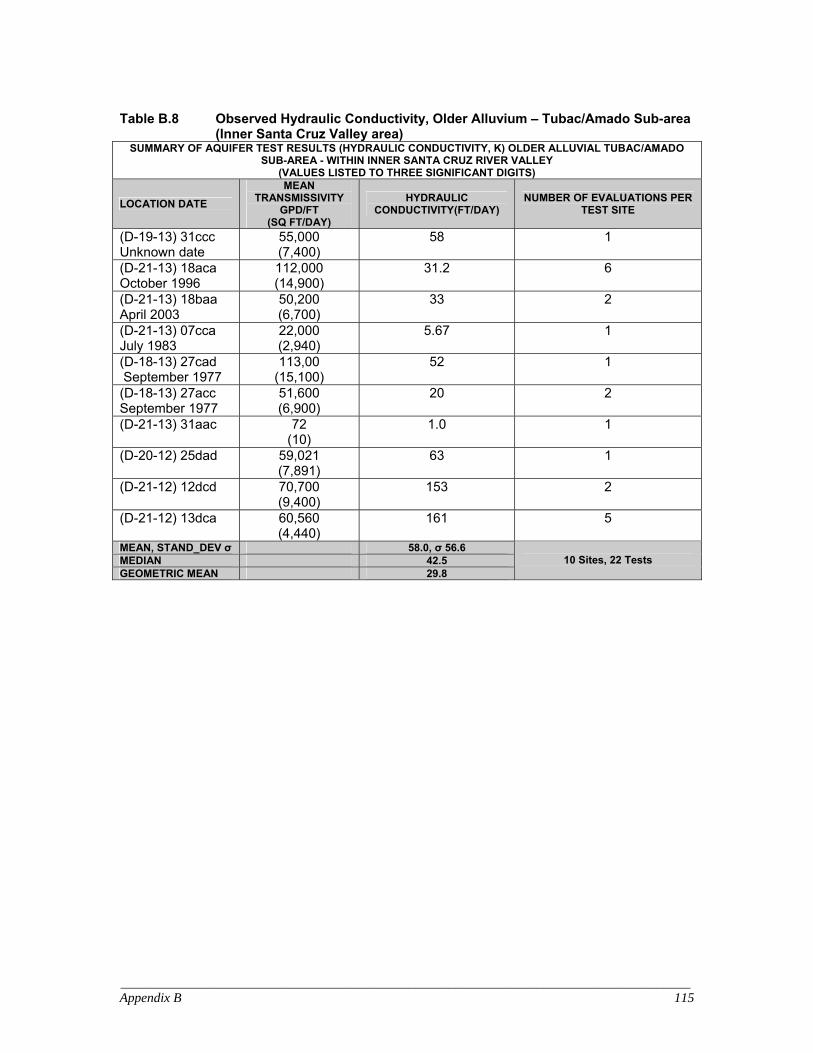
_____________________________________________________________________________________ Appendix B 115
Table B.8 Observed Hydraulic Conductivity, Older Alluvium – Tubac/Amado Sub-area
(Inner Santa Cruz Valley area) SUMMARY OF AQUIFER TEST RESULTS (HYDRAULIC CONDUCTIVITY, K) OLDER ALLUVIAL TUBAC/AMADO
SUB-AREA - WITHIN INNER SANTA CRUZ RIVER VALLEY (VALUES LISTED TO THREE SIGNIFICANT DIGITS)
LOCATION DATE MEAN
TRANSMISSIVITY GPD/FT
(SQ FT/DAY)
HYDRAULIC CONDUCTIVITY(FT/DAY)
NUMBER OF EVALUATIONS PER TEST SITE
(D-19-13) 31ccc Unknown date
55,000 (7,400)
58
1
(D-21-13) 18aca October 1996
112,000 (14,900)
31.2 6
(D-21-13) 18baa April 2003
50,200 (6,700)
33 2
(D-21-13) 07cca July 1983
22,000 (2,940)
5.67
1
(D-18-13) 27cad September 1977
113,00 (15,100)
52 1
(D-18-13) 27acc September 1977
51,600 (6,900)
20 2
(D-21-13) 31aac 72 (10)
1.0 1
(D-20-12) 25dad 59,021 (7,891)
63 1
(D-21-12) 12dcd 70,700 (9,400)
153 2
(D-21-12) 13dca 60,560 (4,440)
161 5
MEAN, STAND_DEV σ 58.0, σ 56.6 MEDIAN 42.5 GEOMETRIC MEAN 29.8
10 Sites, 22 Tests
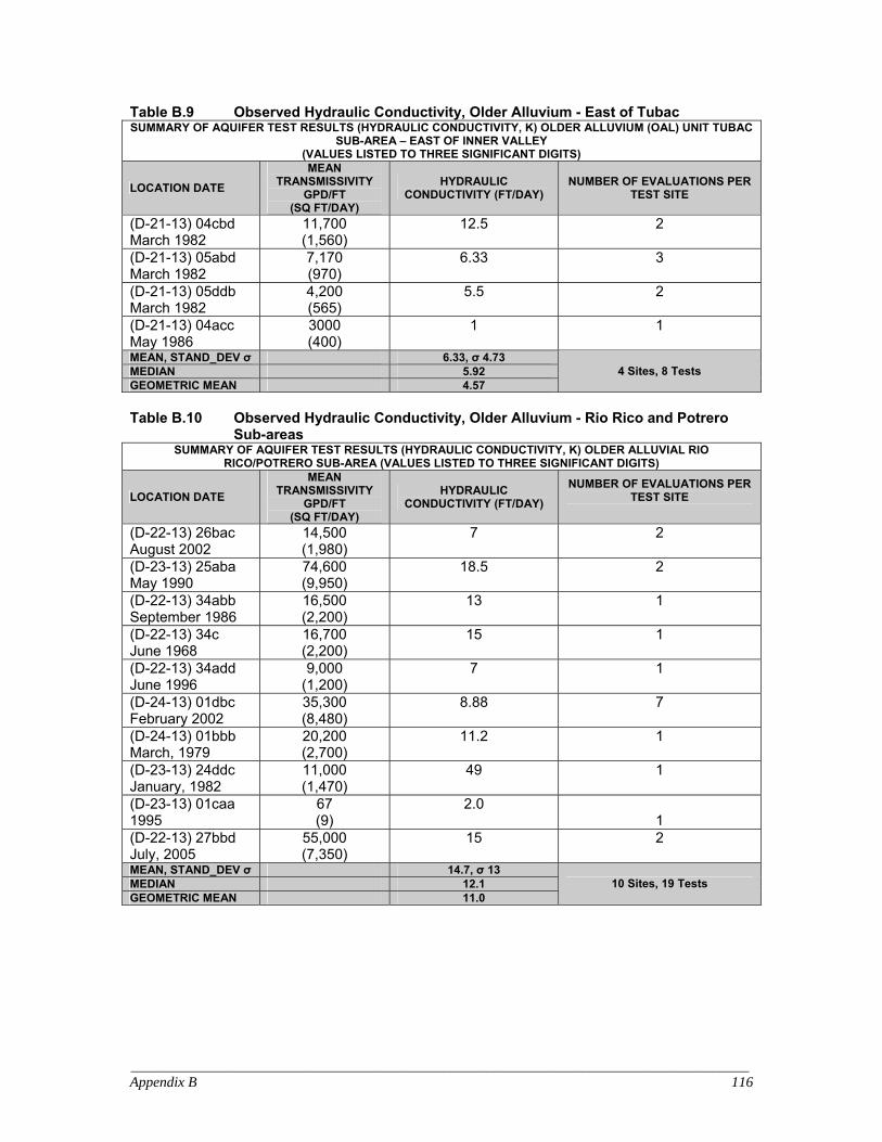
_____________________________________________________________________________________ Appendix B 116
Table B.9 Observed Hydraulic Conductivity, Older Alluvium - East of Tubac SUMMARY OF AQUIFER TEST RESULTS (HYDRAULIC CONDUCTIVITY, K) OLDER ALLUVIUM (OAL) UNIT TUBAC
SUB-AREA – EAST OF INNER VALLEY (VALUES LISTED TO THREE SIGNIFICANT DIGITS)
LOCATION DATE MEAN
TRANSMISSIVITY GPD/FT
(SQ FT/DAY)
HYDRAULIC CONDUCTIVITY (FT/DAY)
NUMBER OF EVALUATIONS PER TEST SITE
(D-21-13) 04cbd March 1982
11,700 (1,560)
12.5 2
(D-21-13) 05abd March 1982
7,170 (970)
6.33 3
(D-21-13) 05ddb March 1982
4,200 (565)
5.5 2
(D-21-13) 04acc May 1986
3000 (400)
1 1
MEAN, STAND_DEV σ 6.33, σ 4.73 MEDIAN 5.92 GEOMETRIC MEAN 4.57
4 Sites, 8 Tests
Table B.10 Observed Hydraulic Conductivity, Older Alluvium - Rio Rico and Potrero
Sub-areas SUMMARY OF AQUIFER TEST RESULTS (HYDRAULIC CONDUCTIVITY, K) OLDER ALLUVIAL RIO
RICO/POTRERO SUB-AREA (VALUES LISTED TO THREE SIGNIFICANT DIGITS)
LOCATION DATE MEAN
TRANSMISSIVITY GPD/FT
(SQ FT/DAY)
HYDRAULIC CONDUCTIVITY (FT/DAY)
NUMBER OF EVALUATIONS PER TEST SITE
(D-22-13) 26bac August 2002
14,500 (1,980)
7 2
(D-23-13) 25aba May 1990
74,600 (9,950)
18.5 2
(D-22-13) 34abb September 1986
16,500 (2,200)
13 1
(D-22-13) 34c June 1968
16,700 (2,200)
15 1
(D-22-13) 34add June 1996
9,000 (1,200)
7 1
(D-24-13) 01dbc February 2002
35,300 (8,480)
8.88 7
(D-24-13) 01bbb March, 1979
20,200 (2,700)
11.2 1
(D-23-13) 24ddc January, 1982
11,000 (1,470)
49 1
(D-23-13) 01caa 1995
67 (9)
2.0 1
(D-22-13) 27bbd July, 2005
55,000 (7,350)
15 2
MEAN, STAND_DEV σ 14.7, σ 13 MEDIAN 12.1 GEOMETRIC MEAN 11.0
10 Sites, 19 Tests

_____________________________________________________________________________________ Appendix B 117
Table B.11 Observed Hydraulic Conductivity, Nogales Formation SUMMARY OF AQUIFER TEST RESULTS (HYDRAULIC CONDUCTIVITY, K) WEST OF TUBAC
(VALUES LISTED TO THREE SIGNIFICANT DIGITS)
LOCATION DATE MEAN
TRANSMISSIVITY GPD/FT
(SQ FT/DAY)
HYDRAULIC CONDUCTIVITY (FT/DAY)
NUMBER OF EVALUATIONS PER TEST SITE
(D-21-12) 24aaa (1984)
3,800 (500)
1.69 2
(D-24-15) 16bdd (1980)
1,575 (210)
0.426 5
(D-24-15) 08ada (1985)
848 (113)
0.174 1
MEAN, STAND_DEV σ 0.763, σ 0.81 MEDIAN 0.426 GEOMETRIC MEAN 0.50
3 Sites, 8 Tests
Estimates of hydraulic storage properties associated with the regional aquifers were less available than estimates of permeability. Table B.12. lists the aquifer storage coefficients and specific yield estimates derived from aquifer tests, where they are known to exist. Table B.12 Aquifer Test Storage Values
SUMMARY OF AQUIFER TEST RESULTS (STORAGE) LOCATION/AQUIFER STORAGE COEFFICIENT SPECIFIC YIELD Rio Rico-Potrero/Oal (D-24-13) 01dbc 0.0002 N/A Rio Rico-Potrero/Oal (D-24-13) 01dbc 0.0001 N/A Rio Rico-Potrero/Yal (D-23-13) 01bd 0.0098 0.19 (19%) Amado/Yal (D-20-13) 06ccb 0.00077 N/A Amado/Yal (D-20-13) 06ccb 0.00087 N/A Amado-Tubac/Oal (D-21-13) 07cca 0.001 N/A Amado-Tubac/Oal (D-21-13) 07cca 0.0006 N/A Amado-Tubac/Oal (D-21-13) 07cca 0.002 N/A Amado-Tubac/Oal (D-21-13) 07cca 0.004 N/A Kino Springs/Nog (D-24-15) 08ada 0.00011 N/A

_____________________________________________________________________________________ Appendix C 118
Appendix C: Properties Associated with the Stream-Aquifer Boundary Stream-aquifer boundary conditions are explained in detail in this Appendix. For all stream parameters, Visual MODFLOW provided linear interpolation between stream segments. For more on the stream boundary see Prudic (1989). See Figure 4.2 for location of stream-aquifer boundary cells, including the location of the five stream segments that were used as flow calibration targets in the model. For reference, the stream-routing boundary equations when the hydraulic head > streambottom, then, Qflow = [(Stream Kz*Stream length* Stream W)/Stream M]*(Hstrm – head); when the hydraulic head is ≤ streambottom then, Qflow = [(Stream Kz*Stream length* Stream W)/Stream M]*(Hstrm – Streambottom). For definition of terms, see below.
Description of Stream-Routing Segments (Length and Position) A total of 22 stream segments are assigned in the stream-routing package. Twelve segments are associated with the main Santa Cruz River Channel, totaling about 27 miles in length. In addition, ten tributary segments bi-sect the main Santa Cruz River channel near confluence areas. Flood flow is introduced in stream segment 1, and, during certain stress periods, in segment 12. All effluent discharge from the NIWTP (IBWC, 1997-2002) is imposed to stream segment 2. Flood flow rates, introduced in segment # 1, were generally based on averaged flow rates recorded at the USGS Tubac Bridge site. The length and position of the simulated streambed were fixed for all steady state and transient solutions based on the approximate stream channel location as defined from topographical and GIS cover maps. The length and position of stream channel change over time, however, these changes aren’t assumed to have significant impacts to the regional-scale groundwater flow system – modeled between 1997 and 2002 - because the high transmissivity of the inner-valley aquifers tend to quickly disperse aquifer stresses, especially over seasonal-based stress-periods. Historical photographs show extensive channelization of the river in the 1950’s. The effects of channelization and incision result in a net reduction in wetted area, and thus greatly reduce recharge in impacted areas. Photos show extreme channelization in the Rio Rico area, and to a lesser extent in the Amado area. Thus for the 1949 – 1959 transient simulation, the net conductance (i.e. width) was decreased along all effected areas of the river.

_____________________________________________________________________________________ Appendix C 119
Table C.1 Segments of the Stream-Routing Boundary SEG. NAME LENGTH
(MILES) COMMENTS
Santa Cruz River/Tributary Confluence Elevation (in Feet) 1 Santa Cruz River 0.59 Introduce Up-stream Flood Flow; (3450, starting
elevation for seg 1) 2 Effluent Discharge 0.3 Quantified Release Rates from NIWTP; (3439) 3 Santa Cruz River 2.5 Between NIWTP and Agua Fria 4 Agua Fria Canyon 0.83 (3394) 5 Santa Cruz River 2.5 Between Agua Fria and Peck Canyons 6 Peck Canyon 1.4 (3339) 7 Santa Cruz River 3.9 Between Peck and Josephine Canyons 8 Josephine Canyon 1.0 (3269) 9 Santa Cruz River 4.8 Between Josephine and Mavis Canyons 10 Mavis Canyon 0.52 (3185) 11 Santa Cruz River 0.24 Between Mavis Canyon and Tubac Creek 12 Tubac Creek 0.82 (3177) 13 Santa Cruz River 3.6 Between Tubac Creek and Cottonwood Canyon 14 Cottonwood Canyon 0.54 (3140) 15 Santa Cruz River 3.7 Between Cottonwood and Diablo Canyons 16 Diablo Canyon 0.78 (3083) 17 Santa Cruz River 0.24 Between Diablo and Montosa Canyons 18 Montosa Canyon 0.79 (3078) 19 Santa Cruz River 2.5 Between Montosa Canyon and Sopori Wash 20 Sopori Wash 1.9 (3024) 21 Santa Cruz River 1.3 Between Sopori Wash and Arivaca Junction; (3004) 22 Santa Cruz River 0.63 Between Arivaca Junction and Elephant Head
Bridge; (2993, ending elevation for seg 22) 1 – 22 TOTAL LENGTH ~ 27 MILES NIWTP TO ELEPHANT HEAD BRIDGE
Streambed Elevation Transient changes to the stream channel elevation can have significant impacts to inner valley groundwater levels because of the stream-aquifer interaction (Webb and Leake, 2005). With MODFLOW land surface elevations are important when representing head-dependant boundaries referenced to land surfaces, such as the stream-routing package and ET package. Because the streambed altitude functions as reference elevations for stream-aquifer interactions, the assigned streambed elevations have a direct effect on groundwater levels throughout the inner valley. Streambed elevations assigned at major tributary confluences are listed in Table C.1. Inter-cell streambed elevations bisecting the 12 stream segments along the river were computed by linear interpolation (Visual MODFLOW, 2003). The inclusion of numerous bisecting segments along the main Santa Cruz River channel provide good elevation control between major confluence points. Assigned streambed elevations were initially based on digital elevation model (DEM, grid spacing of 15 and 30 meters, USGS, 1997). However, direct application of DEM elevations resulted in biased simulated groundwater levels where simulated heads generally exceeded observed heads between Tumacacori and Chavez Siding. Suspect areas were re-evaluated by survey-grade GPS (Tatlow, 2004), and updated streambed elevations were applied in the model. The resurveyed

_____________________________________________________________________________________ Appendix C 120
elevations improved simulated hydraulic heads but did not completely remove the simulated head bias observed between Tumacacori and Chavez Siding. During the model development phase alternative conceptual models were developed to examine the impact of different streambed gradients associated with the stream boundary. Solutions to the alternative streambed gradient models were similar to base-case parameter estimates, and also show similar parameter reliability. [Note that long-term tributary recharge was imposed into the model by specified flux through the recharge package.] Some sections of the stream channel have changed in elevation over time. Downstream from the model area, streambed elevations have risen about 10 feet between 1929 and 1985 (Parker, 1993). Areal photos from the 1950s reveal the “straightening” effects of extensive channelization and incision along the river. Extreme fall and winter flooding between the 1960’s and 2001 has refilled stream channels with sediment that had been previously scoured away during earlier channelization. Parker (1993) suggests the current system experiences periods of both aggradation and degradation. A recent analysis by the U.S. Geologic Survey shows that the relative elevation of the streambed channel at Tubac has increased by about five feet between 1995 and 2003 (Fritzinger and Evans, 2004). However, it is unclear if other segments along the river have similarly changed. Streambed elevations were not modified for the 1949-1959 simulation because of a lack of data; this uncertainty remains problematic.
Streambed Width (Stream W) The streambed-width parameter (stream W) is based on field data and regression analysis. Over winter baseflow periods (1997-2002), stream W was assigned at streambed widths between 20 and 30 feet, depending on location and flow. Over flood-dominated stress periods, stream W was adjusted with respect to streambed width-discharge relations established at the Tubac Bridge site, and at the Santa Cruz River Nogales site. CDM (1999) developed the following width-discharge relation for the Tubac and Nogales gauges, where Stream W = 6.62Q0.5084, R2 = 0.9068. For pre-development steady state conditions, stream W was assigned a value of 20 feet at stream segment one, increased to 25 feet (near Tumacacori and Tubac), and linearly-reduced to 5 feet north of Amado, reflecting infiltration north of Tubac; the assumptions associated with the assignment of pre-development stream W remain difficult. To represent the straightening of the streambed channel observed in the 1950s, the net streambed conductance was decreased by reducing the channel width to five feet over all non-flood periods. Note that the straightening of an otherwise naturally meandering channel results in a decrease in streambed length and effective width; however, decreasing the width has the same net effect with respect to the linear streambed conductance term; thus, for simplicity only this term was adjusted (therefore note that the length of the streambed was not modified). Also note/recall that there was no effluent discharge in the 1950’s. However, there may have occasionally been some minor runoff and groundwater discharge components along the river during baseflow periods; therefore the stream boundary condition remained active during simulations. During moderate flood periods, the stream width was increased to 25 feet in the Rio Rico area, and 50 feet in the Tubac and Amado areas. During the two extreme floods periods (i.e.,

_____________________________________________________________________________________ Appendix C 121
August 1954, and August 1955), the simulated flood stream width was assigned between 150-200 feet. Note that all stream-aquifer boundary conditions assigned during the 1949-1959 simulation have a high degree of uncertainty due to lack of data. Table C.2 Observed and Assigned Flow and Stream Width
STRESS PERIOD OBSERVED MEAN FLOW, STANDARD DEVIATION, σ,
AT TUBAC (CFS)
CALCULATED STREAMBED WIDTH (FEET) AT TUBAC 6.62Q 0.508, R2 = 0.907
ASSIGNED STREAMBED WIDTH,
W, (FEET) 1Baseflow 25, σ <5 34 20-30
3 53, σ 38 50 40-50 5 46, σ 84 46 40 10 59, σ 105 53 40-60 15 24, σ 25 33 25 16 542, σ 1100 162 160-125 17 84, σ 15 63 60-70 18 54, σ 49 50 40-60 19 18, σ 14 29 25-30 20 21, σ 20 31 25-30 25 14, σ 50 25 25-30
1Stress Periods: 1, 2, 4, 6, 7, 8, 9, 11, 12, 13, 14, 21, 22, 23 and 24.
Streambed Conductivity (Stream Kz) To determine the steady recharge rate and information about system parameter reliability, recharge cells were assigned along the losing reach of the Santa Cruz River between Tubac and Elephant Head Bridge over steady state and quasi-steady conditions. Recharge along the Santa Cruz River along with the other system parameters including hydraulic conductivity, MFR and tributary recharge, and subsurface recharge were all estimated as independent parameters. See Appendix F. Non-linear regression results indicate that the optimal steady state recharge rate between Tubac and Elephant Head Bridge is approximately 19 cfs, and that the associated standard deviation is about 6 cfs along this reach. The inversion statistics show high correlation between recharge along the Santa Cruz River and the underlying hydraulic conductivity associated with the older alluvial unit in the Tubac and Amado areas (Koal_North). To improve parameter reliability, recharge cells located between Tubac and Elephant Head Bridge were replaced with the stream-routing (SR) head-dependent boundary (Prudic, 1989). The SR boundary contains physical parameters that can be cross-checked against calibrated values including streambed width, stage and length. In addition, the magnitude of streambed conductivity, stream Kz, can be compared with other, field-derived values (Lacher, 1996) for consistency. [Note that direct recharge could not be imposed between the NIWTP and Tubac due to the nearly-hydrostatic conditions (i.e., locations where the water table elevation is nearly equal to the stream-stage elevation) that prevail along this reach, where the river goes through a series of gains and losses; this condition, effectively requires a head-dependant boundary for simulation purposes]. Optimized steady state recharge rate (using recharge cells) correspond to a composite, global stream Kz value of 1.7 feet/day, which were then assigned over baseflow periods in the transient simulation. Calibrated values of streambed Kz over baseflow conditions

_____________________________________________________________________________________ Appendix C 122
are consistent with empirical data and other modeling investigations (Lacher, 1996; Calver, 2002). Streambed Kz was relatively sensitive between Tubac and Elephant Head Bridge, but was not as sensitive between the NIWTP and Tubac. Immediately downstream from the NIWTP, streambed Kz has distinctive hydraulic properties over baseflow conditions. For all viable conceptual models (1997-2002), a clogging layer was necessarily assigned over the first few miles downstream of the NIWTP. Nutrient-rich effluent promotes development of a clogging layer, which consequently impedes vertical infiltration. Discharged effluent is characterized by high-levels of biological oxygen demand (BOD) and ammonia, and concentrations are highest immediately downstream from the NIWTP (Lawson, 1995; Stromberg, et al., 1993). The clogging layer feature was hydraulically represented in the model by assigning a stream Kz of 0.1 feet/day along affected stretches. Failure to incorporate the clogging-layer results in unrealistically-low hydraulic head decline rates near Rio Rico (south) in the transient simulation. The clogging layer was necessarily “removed” over all flood-dominated stress-periods due to scour, and was then “reset” for subsequent baseflow conditions not affected by flood scour. BOD and ammonia concentrations rapidly decline downstream from the NIWTP (Lawson, 1995; Stromberg, et al, 1993) and reduce the hydraulic impeding effect of the clogging layer. For baseflow conditions, the magnitude of the clogging-layer, Kz, was linearly increased from 0.1 to 1.7 feet/day along the 2.5-mile stretch of river between the Agua Fria and Peck Canyon confluences. Downstream from Peck Canyon, the streambed Kz was assigned a value of 1.7 feet/day reflecting a more direct stream-aquifer interaction. The location of the clogging layer (and its linear change downstream) was relatively insensitive over a couple of miles, either upstream or downstream, of the assigned location. However, the clogging layer could not be extended north of the Josephine Canyon confluence (1997-2002) without causing significant model error. In reality, the clogging layer probably extends and retracts over periods of drought, and according to season. For the transient simulation, stream Kz was calibrated to hydraulic head changes over flood-dominated based periods. For moderately-large flood periods, including the 1998 El Nino events (i.e., February to April 1998), and the active monsoons of 1998 and 1999, stream Kz was increased to 2.0 feet/day for all stream segments along the river. The increase in stream Kz over flood-dominated stress periods is assumed to result from scouring of the clogging layer. Over extreme flood periods, i.e., the fall/winter of 2000-2001, stream Kz was calibrated to 3.0 feet/day, identical to empirical values obtained by Lacher (1996) over a similar stretch of effluent-dominated river, i.e. Santa Cruz River near Tucson. The consistency of observed and calibrated stream Kz reinforces the certainty of the calibrated values. Stream Kz was “reset” for nominal baseflow conditions following flood-scouring events. The timing associated with the re-development of the clogging layer stream is discussed by Lacher (1996). All stream Kz values assigned during the 1949-1959 simulation are consistent with the calibrated values determined in the 1997-2002 simulation, i.e. average monsoon stream Kz = 2.0 feet/day; the extreme flood periods, stream Kz = 3.0 feet/day.

_____________________________________________________________________________________ Appendix C 123
[Note: Inspection of head and flow data collected between the spring 2002 and 2006, suggest that the lack of flood scour has reduced the hydraulic communication between the stream and water table aquifer downstream from the NIWTP past the Peck Canyon confluence. The data suggests that the less active monsoons (i.e. 2001- 2005), combined with the lack of significant fall/winter flooding since early 2001, has reduced the episodes of periodic scouring required to facilitate a more direct stream-aquifer connection. This suggests that the calibrated baseflow stream Kz, assigned at 1.7 feet/day during the 1997-2002 transient simulation, may actually need to be reduced for simulations covering the periods between 2002 and 2006].
Streambed Thickness (Stream M) Stream M is equal to the streambed top minus the streambed bottom (strmbot) and is a component of the streambed conductance term. The elevation of the streambed bottom defines the reference where flow occurs 1) at a rate proportional to the difference between stream stage (Hstrm) and aquifer head (either gaining or losing) as defined by the conductance, when aquifer head, h > stream bottom; or 2) infiltrates at fixed rates (i.e., h <= strmbot), as defined explicitly by the streambed conductance and the altitude of the stage. Alternative conceptual models were developed to evaluate stream M in coordination with stream Kz over steady state, quasi-steady and transient conditions. Accordingly, stream M was optimally calibrated to a value of five feet. Stream M assigned at values greater or less than five feet, along with coordinated/calibrated changes in Kz, yielded solutions that had either larger model error, or, increasingly unrealistic solutions. Applying a stream M equal to 5.0 feet resulted in a slight head bias near Tubac. Although a thinner stream M equal to 2.5 feet, produces less head bias near Tubac, thicker values of stream M result in less oscillation between groundwater discharge and recharge between the NIWTP and Tubac; this thinking is currently more consistent with the conceptual model, which assumes that a more continuous rate of groundwater discharge occurs along this reach (although it’s acknowledged that this reach experiences both gaining and losing reaches between the NIWTP and Tubac during the winter baseflow periods between 1997-2002; see Scott et.al, 1995). Thus the assignment of stream M equal to 5 feet reflects a tradeoff between head and flow residuals, as well as the performance of simulated gains and losses along the reach between NIWTP and Tubac. Stream M is most sensitive between the NIWTP and Tubac where groundwater and surface water interactions are complex and include both gaining and losing reaches over winter baseflow periods. The reach between the NIWTP and Tubac is represented in the model by the head-dependent boundary function (Prudic, 1989) mostly within the linear zone, where the water table and stream surface elevations are similar. Along the predominantly losing reach between Tubac and Elephant Head Bridge, stream M was not as sensitive because simulated heads tended to fall below stream bottom elevations where the infiltration rate is primarily a function of streambed conductance. A stream M equal to 5 feet was retained throughout all stream segments, and was not modified for the pre-development period, or during the1949-1959 simulation. Thus for the reaches north of Tubac, the assignment of stream M equal to five feet was an assumption based the more sensitive calibration between the NIWTP and Tubac.

_____________________________________________________________________________________ Appendix C 124
Table C.3 Assigned Streambed Conductivity STRESS PERIOD ASSIGNED STREAMBED CONDUCTIVITY (FEET/DAY)
1Baseflow (1997-2002) 1.7 1bBaseflow Pre-development, Circa 1880 2.0
2Clogged Baseflow 0.1 3 2.0 5 2.0
10 2.0 15 1.7 16 3.0 17 3.0 18 2.0 19 1.7 20 1.7 25 1.7
1Stress Periods: 1, 2, 4, 6, 7, 8, 9, 11, 12, 13, 14, 21, 22, 23 and 24. 1bIncludes all stream segment lengths. 2Between NIWTP and Agua Fria Confluence only; linearly increases from 0.1 to 1.7 between the Agua Fria and Peck Canyon confluence for baseflow conditions
Stream Stage (Hstrm) The elevation of Hstrm assigned over baseflow and flood-dominated periods was based on stage-discharge relations established at the Tubac Bridge Site. The stage-discharge relation at Tubac assumes a trapezoidal-shaped stream channel geometry. Measured surface water flow, stream width and cross-sectional area, recorded at the Tubac Bridge site from September 1995 to May 2003 was used to determine the approximate Hstrm (USGS, 1995-2003). The following stage-discharge regression-relation was established: Hstrm = 0.237Q 0.370, and R2 = 0.858, where Q equals the mean surface water flow rate recorded over the respective stress period at the Tubac gauge (USGS, 1997-2002), and Hstrm equals the depth in feet. In addition, CDM (1999) developed the following depth-discharge relation for the Tubac and Nogales gauges, where Hstrm = 0.1964Q 0.2421, and R2 = 0.7842. Assuming average baseflow conditions of 20 cfs, the calculated Hstrm, based on the Tubac and CDM stage-discharge models, was 0.72 and 0.40 feet, respectively. Manual seepage measurements recorded along the Santa Cruz River during winter baseflow periods (1997-2002) show similar Hstrm values, typically between 0.3 and 0.7 feet. For modeling purposes, the Hstrm was assigned an averaged, global value of 0.5 feet above the streambed top for all baseflow conditions. Because both rating curves as well as manual seepage measurement show similar and consistent stages, it’s assumed that the average winter baseflow Hstrm value (0.5 feet) was assigned with a relatively- high degree of certainty over these periods; however it is acknowledged that Hstrm varies over time and space about this average value along the ~27 mile reach of the Santa Cruz River. Higher uncertainty exists over flood-dominated periods, where Hstrm was calibrated to fit temporal heads changes over time; nonetheless, the calibrated Hstrm is reasonably consistent with regression values.

_____________________________________________________________________________________ Appendix C 125
Table C.4 Observed and Assigned Flow and Stream Stage
STRESS PERIOD
OBSERVED MEAN FLOW, STANDARD DEVIATION
AT TUBAC (USGS) (CFS)
ASSIGNED INFLOW AT SEGMENT 1
(CFS)
CALCULATED FLOOD STAGE
SEGMENT 1 (FEET)
ASSIGNED HSTRM ABOVE
BASEFLOW STAGE (FEET)
Baseflow ~ 25 0 0.4 – 0.7 0.5 3 53, σ 38 50; 25* 1.2 2.0 5 46, σ 84 50; 25* 1.2 2.0 10 59, σ 105 60; 50* 1.2 2.0 15 24, σ 25 25; 10* 1.0 1.0 16 542, σ 1100 500 2.4 12.0 – 23.0 17 84, σ 15 85 1.2 2.0 18 54, σ 49 60 1.1 2.0 19 18, σ 14 25 0.70 1.0 20 21, σ 20 30 0.70 1.0 25 14, σ 50 20 0.63 1.0
1Hstrm assigned downstream from segment 13 (Tubac); 2Hstrm assigned between segment 1 (NIWTP) and segment 12 (Tubac Creek); *Imposed tributary flow at stream segment # 12 near Tubac to accommodate additional, contributing
flows north of Tubac.
An alternative stream-aquifer boundary condition was modeled whereby the Manning’s N option in Prudic (1989) was activated; this option calculates the stage, in part, as a function of flow in the river. An optimal stream M of 2.5 feet was calibrated for this condition over steady state and transient conditions, although a stream M of 5 feet also provides viable solutions. Results of applying the Manning’s N option was very similar - both in the solution, i.e. optimal parameter values, heads and flows, as well as in the inversion statistics - to the other viable models discussed in Chapter 6, but requires an additional model parameter, Manning’s N coefficient (assigned herein at 0.04).

_____________________________________________________________________________________ Appendix D 126
Appendix D: Observed Steady State Groundwater Levels Table D.1 Quasi-Steady Groundwater Elevations Winter 1997-1998 LOCATION NOVEMBER/
DECEMBER 1997 JANUARY 1998 FEBRUARY/MARCH 1998
Arivaca Junction (D-19-13) 36acd
2978 2979 2979
Amado(D-20-13) 07acd 3044 3045 3045 Tubac/Chavez Siding (D-20-13) 32bcc
3126 3127 3127
Tubac (D-21-13) 05ccb 3150 3150 Tumacacori (D-21-13) 30dca 3238 3238 Rio Rico North (D-22-13) 09bdd3 3307 3308 Rio Rico North(D-22-13) 09dcc 3317 3317 3317 Rio Rico- Central (D-22-13) 22bcb
3358 3358 3358
Rio Rico South(D-23-13) 01bbd 3410 3411 3413 All units in feet.
Table D.2 Quasi-Steady Groundwater Elevations Winter 1998-1999 LOCATION NOVEMBER/
DECEMBER 1998 JANUARY 1999 FEBRUARY/MARCH 1999
Elephant Head (D-19-13) 29bcc 2965 2965 2965 Arivaca Junction (D-19-13) 36acd
2982 2982 2982
Amado(D-20-13) 06ccb3 3030 3030 3029 Amado(D-20-13) 07acd 3048 3048 3047 Chavez Siding-East (D-20-13) 33bca3
3123 3122
Tubac/Chavez Siding (D-20-13) 32bcc
3126 3125 3125
Tubac (D-21-13) 05ccb 3149 3149 Tubac-East (D-21-13) 05adb 3149 3149 Tubac-West (D-21-13) 18cdb2 3199* 3199 Tumacacori (D-21-13) 30dca 3238 3238 Rio Rico–North(D-22-13) 09dcc 3316 3316 Rio Rico–South(D-23-13)01bbd 3420 3419 3418 Rio Rico– Southeast (D-22-13) 25ddd
3423 3423 3422
All units in feet. *Measured 9/16/1998.

_____________________________________________________________________________________ Appendix D 127
Table D.3 Quasi-Steady Groundwater Elevations Winter 1999-2000 LOCATION NOVEMBER/
DECEMBER 1999 JANUARY
2000 FEBRUARY
2000 MARCH 2000
Elephant Head (D-19-13) 29bcc 2965* 2965 Arivaca Junction (D-19-13) 36acd
2981 2981 2980 2980
Amado (D-20-13) 07acd 3046 3045 3044 3044 Tubac/Chavez Siding (D-20-13) 32bcc
3124 3123**
Tubac (D-21-13) 05ccb 3149 3150 Tubac-West (D-21-13) 18cdb2 3199*** 3199 Tumacacori (D-21-13) 30dca 3238 3238 3238 3238 Rio Rico-North (D-22-13) 09dcc 3316 3315 3315 3315 Rio Rico-South(D-23-13) 01bbd 3419 3418 3416 3416 *Extrapolated from 8/18/1999 measurement. **6/13/2000. ***7/14/1999. All units in feet. Table D.4 Quasi-Steady Groundwater Elevations Winter 2001-2002 LOCATION NOVEMBER/
DECEMBER 2001 JANUARY 2002 FEBRUARY 2002
Elephant Head (D-19-13) 29bcc 2965 2966 2967 Arivaca Junction (D-19-13) 36acd
2983 2982 2983
Amado (D-20-13) 07acd 3048 3050 3050 Chavez Siding (D-20-13) 32bcc 3126 3126 3126* Tubac (D-21-13) 05ccb 3148 3150 Tumacacori (D-21-13) 30dca 3239 3239 Rio Rico-North (D-22-13) 09dcc 3318 3318 3318 Rio Rico-South (D-23-13) 01bbd 3423 3423 3422 *03/26/2002. All units in feet.

_____________________________________________________________________________________ Appendix D 128
Table D.5 Observed Groundwater Levels, Outside Santa Cruz River Valley LOCATION – OUTSIDE INNER VALLEY WINTER, 1999 WINTER, 2000 NW of Arivaca Junction, (D-19-12) 28 bda 2977* 2976 East of Elephant Head, (D-19-13) 34 cad 2995* 2994 Southeast of Amado, (D-20-13) 20cbb 3086 3085 Northwest of Tubac, (D-20-12) 26cad 3119 3118 West of Tubac, (D-21-13) 18cdb2 3199 3200 West of Carmen, (D-21-12) 24aaa 3226 3225 East of Amado, (D-20-13) 09ddd 3209 3209 Atascosa Ranch, (D-22-13) 19dcc 3324 3323 Upper Sonoita Creek, (D-22-13) 25ddd 3421 3421 South of NIWTP, (D-23-13) 12acd 3465 3465 Potrero Sub-area, (D-23-13) 15cbc2 3472* 3471 SW Potrero Sub-area, (D-23-13) 29ccc 3699 3700 1997 2003 Sopori Wash, (D-20-12) 05adb2 3204** 3204 West of Carmen, (D-21-12) 24aaa 3225 3225 Atascosa Ranch, (D-22-13) 19dcc 3324 3323 South of NIWTP, (D-23-13) 12acd 3462 3462 SW Potrero Sub-area, (D-23-13) 29ccc 3698 3699 Northwest of Tubac, (D-20-12) 26cad 3121 3119 1998 2000 2005 East of Amado, (D-20-13) 09DDD 3209 3208 3208 West of Tubac, (D-21-13) 18CDB2 3200 3200 3199 *Interpolated from January 1995 measurement; **November, 2001. All units in feet.

_____________________________________________________________________________________ Appendix D 129
Table D.6 Long-term Observed Groundwater Levels Location 1982 2000 NW of Arivaca Junction (D-19-12) 28bda 32976 2976 Arivaca Junction (D-19-13) 32abc Arivaca Junction (D-20-12) 36adb
2982 3140
2988 3134
Sopori – west of fault, (D-20-12) 05cbb Sopori – east of fault (D-20-12) 03bbb
3252 3008
3252 53006
Amado - south, (D-20-13) 30bcd Amado, (D-20-13) 19ccc Amado - north, (D-20-13) 06cba
3096 3086 3023
3099 3090 3026
Agua Linda, east (D-20-13) 20cbb 3085 3085 East of Amado/Tubac, (D-20-13) 09ddd East of Amado/Tubac, (D-20-13) 25cab East of Amado/Tubac, D-20-13) 36acd
23205 3762 3818
3208 3769 3814
Cottonwood Canyon, (D-20-13) 33bca 3123 3125 Tubac (D-21-13) 05daa Tubac, (D-21-13) 07acd Tubac (D-21-13) 08cad1
3165 3170 3175
3165 3170 3174
Tubac - Northwest, (D-21-12)13ada 3192 3190 Carmen, (D-21-13) 18cdb1 Carmen, (D-21-13) 19dbc
3198 3218
3198 3214
Tumacacori, (D-21-13) 30bca Tumacacori, (D-21-13) 32bc
3217 3258
3215 3256
Peck Canyon - west, (D-22-13) 19dbd 43321 3318 Rio Rico - north, (D-22-13) 09 ac Rio Rico - north, (D-22-13) 09 cda Rio Rico - north, (D-22-13) 22 bcb Rio Rico - central, (D-22-13) 27aab Rio Rico - central, (D-22-13) 34add Rio Rico - south, (D-22-13) 35dbc Rio Rico - south, (D-23-01) 01cab
3310 3316 3360 3372 3389 3410 43422
3309 3317
53358 3373 3389 3407 3423
Sonoita Creek, (D-22-13) 25ddd 3418 3421 South of the NIWTP, (D-23-13) 12acd South of the NIWTP, (D-23-13) 13dad2 South of the NIWTP, (D-23-13) 24daa
23461 3510 3544
3464 3507 3540
West of NIWTP, (D-23-13) 08cb 3521 13522 5measured 1998; 41987; 31979; 2Early 1970’s; 12007 - surface water effect in 2000. All units in feet. Location – Inner Valley ~1940 ~2000 Amado, (D-20-13) 19ccc 3087 3090 Amado – south, (D-20-13) 31aac 3118 3118 Chavez Siding, (D-20-13) 32bcc 3121 3125 Rio Rico – north, (D-22-13) 09ac 3304 3309 Rio Rico – north, (D-22-13) 09da 3307 3315 Rio Rico – central, (D-22-13) 16dc 3341 3340 Rio Rico – central, (D-22-13) 27aab 3364 3370 Rio Rico – south, (D-22-13) 35 dcd 3413 3420

_____________________________________________________________________________________ Appendix E 130
Appendix E: Observed Flows See Figure 4.2 for location stream-aquifer boundary cells, including the five segments used as calibration targets in the regression. Table E.1 Observed Continuous Flow Rates Between NIWTP and Tubac, 1995-2002.7
NET WINTER BASEFLOW RATES RECORDED ALONG THE SANTA CRUZ RIVER BETWEEN THE NIWTP AND TUBAC (CONTINUOUS RECORDING, IBWC AND USGS)
NET FLOW REACH (Segments 1 – 3, See Figure 4.2) Between the NIWTP and Tubac
TIME (WINTER PERIOD); MONTHLY AVERAGE OF DAILY FLOW
-6.62 -6.22 -6.52
December, 1995 January, 1996 February, 1996
1.12 -5.22 -9.82
December, 1996 January, 1997 February, 1997
-4.72 -6.92
December, 1997 January, 1998
-2.62 -2.72 -6.02
December, 1998 January, 1999 February, 1999
-5.42 -4.22 -5.52 -3.92
November, 1999 December, 1999 January, 2000 February, 2000
-4.02 -3.32 -5.22
December, 2001 January, 2002 February, 2002
MEAN = -4.9 cfs, STANDARD DEVIATION = 2.3 cfs WINTER BASEFLOW RATES, 1995-2002 MEAN = -4.5cfs, STANDARD DEVIATION = 1.3 cfs WINTER BASEFLOW RATES, 1997-2002
MEAN = -4.8cfs, STANDARD DEVIATION = 0.82 cfs NOVEMBER 1999 – FEBRUARY 2000: SYNOPTIC, STEADY STATE PERIOD
2IBWC, 1995-2002, USGS, 1995-2002; 2“-” indicates gaining flow reach. Note that the net flow rates do not reflect evaporation losses along stream surface, estimated at 0.5 cfs (Scott, et al, 1996). No significant runoff was observed during these periods. Note that these rates are net flow rates from the aquifer to the stream (or stream to aquifer) , and do NOT represent surface water flow rates.

_____________________________________________________________________________________ Appendix E 131
Table E.2 Observed Manual Flow Rates Between NIWTP and Tubac, 1992-2002 NET WINTER BASEFLOW RATES DISCRETELY/MANUALLY-RECORDED ALONG THE SANTA CRUZ RIVER
BETWEEN THE NIWTP AND TUBAC NET FLOW REACH (Segments 1,2 and 3,See Figure 4.2)
NET FLOW: TIME (WINTER PERIOD)
Rio Rico Bridge to Tumacacori -5.43 November, 1992 NIWTP to Tumacacori -3.24 NIWTP to Tubac -4.74
December, 1995 December, 1995
Rio Rico Bridge to Tumacacori -105 Rio Rico Bridge to Tumacacori -5.55 Rio Rico Bridge to Tumacacori -8.45 Rio Rico Bridge to Tumacacori -7.55
December, 1995 December, 1995 January, 1996 February, 1996
Rio Rico Bridge to Tumacacori -6.85 Rio Rico Bridge to Tumacacori -6.05
January, 1997 February, 1997
Rio Rico Bridge1 to Tubac -1.71 Rio Rico Bridge1 to Tubac -2.61 Rio Rico Bridge1- to Tubac -7.81
December, 1997 January, 1998 February, 1998
Rio Rico Bridge1 toTubac -4.91 Rio Rico Bridge1 toTubac -8.51 Rio Rico Bridge1 toTubac -7.51
November, 1998 December, 1998 January, 1999
Rio Rico Bridge 1 to Tubac -6.01 January, 2000 Rio Rico Bridge to Carmen -3.41a February, 2002 MEAN, σ (STANDARD DEVIATION) -5.9, σ 2.3 WINTER BASEFLOW RATES, 1992-2002 MEAN, σ (STANDARD DEVIATION) -5.3, σ 2.6 WINTER BASEFLOW RATES, 1997-2002 1Nelson and Erwin, 2001; 1aADWR, 2002; 3Lawson, 1995; 4 Scott, et al., 1996; 5FOSCR, 1995-1997. All units in cfs; “-” indicates gaining flow reach. Rates do not account for evaporation losses along stream surface estimated at 0.5 cfs (Scott, et al., 1996). Rio Rico1 recorded at Palo Parado. Note that Rio Rico Bridge is ~ 1 mile downstream from NIWTP discharge point. . Note that these rates are net flow rates from the aquifer to the stream (or stream to aquifer) , and do NOT represent surface water flow rates. Table E.3 Conceptual Model Flow Rates Between NIWTP and Tubac, January 2000
MODEL REACH Segment 1 Segment 2 Segment 3 Observation 01a -6.01 01 Observation -5.52
1Measured baseflow January 26th, 2000 (Nelson and Erwin, 2001; 1aRate adjusted for NIWTP/Rio Rico Bridge site due to diurnal cycle of effluent discharge; 2IBWC, 2000; USGS, January, 2000. All units in cfs; “-” indicates gaining reach. Note that values do not reflect evaporation losses along stream surface, estimated at about 0.5 cfs (Scott, et al., 1996). Note that these rates reflect net flows, and do not represent the total cumulative individual losses and individual gains accrued along these reaches; finer spatial flow resolution is unknown.. Note that these rates are net flow rates from the aquifer to the stream (or stream to aquifer) , and do NOT represent surface water flow rates.

_____________________________________________________________________________________ Appendix E 132
Table E.4 Observed Flow Rates Between Tubac and Elephant Head Bridge NET FLOW (INFILTRATION) RATES RECORDED NORTH OF TUBAC ALONG THE SANTA CRUZ RIVER OVER
NON-SUMMER PERIODS TIME FROM TUBAC TO AMADO
Segment 4 FROM AMADO TO EH
Segment 5 12 14
December 12, 1997 January 7, 1998 February 14, 1998 18
14 8* 11 10* 14 11* 7.6 5.0 9.4 5.4
November 19, 1998 December 16, 1998 January 14, 1999 March 2, 1999 April 7, 1999 April 30, 1999 11 3
8.3 11 October 27, 1999 January 26, 2000 7.2 2.2
13 February, 12, 2001 March 29, 2001 12 February 27, 2002 12** 5.8** MEAN, σ (STANDARD DEVIATION) 12, σ 3.2 17.1, σ 4.2
27.8, σ 3.8 36.8, σ 3.3
Source: Nelson and Erwin, 2001; *estimated flow. **Interpolated measurement between along Santa Cruz River Tubac (Baily Crossing) and Elephant Head Bridge. All units in cfs. 1Not including estimated flow; 2Includes all flow; 3Does not include 2001 flows. Note that σ means standard deviation. Note that these rates are net flow rates from the aquifer to the stream (or stream
to aquifer), and do NOT represent surface water flow rates. Table E.5 Conceptual Model Flow Rates
MODEL REACH Segment 1 Segment 2 Segment 3 Segment 4 Segment 5 Conceptual steady state flow rates, winter, baseflow periods, 1997-2002
Observation 0, σ = 1 -6, σ = 1 0, σ = 1 12, σ = 4 7, σ = 4 Observation -6*, σ =2.5* 12, σ = 4 7, σ = 4
Conceptual steady state flow rates, winter, baseflow periods, Pre-development period Estimate -1, σ = 3 -6, σ = 3 -1, σ = 3 12, σ = 6 4, σ = 6 Estimate -8*, σ = 5* 12, σ = 6 4, σ = 6
Conceptual Flow rate in cfs; Standard Deviation, σ. “-” indicates gaining reach. Note that these rates are net flow rates from the aquifer to the stream (or stream to aquifer) , and do NOT represent surface water flow rates. *Alternative statistic assigned when applying one net flow rate between segment 1 and Tubac: Yields similar model solution and reliability statistics. The “final” model solution applied the higher spatial flow resolution (i.e., three net flow zones between segment 1 and Tubac) as determined by both observed continuous flow and seepage data.

_____________________________________________________________________________________ Appendix F 133
Appendix F: Inverse Model Statistics This appendix provides parameter estimation results and associated statistics from the non-linear regression. Listed below are indicators of model performance and measures of parameter relations including: 1) The 95% confidence intervals; 2) parameter correlation coefficients; 3) parameter composite sensitivities; 4) normalized eigenvectors of the parameter covariance matrix; 5) and singular value decomposition of the sensitivity (Jacobian) matrix. For more information about the inverse model statistics there are many helpful references including (but not limited to): Carrera (1984); Carrera and Neuman Parts 1 and 3 (1986); Carrera et al. (2005); Cooley and Naff (1990); Menke (1989), Poeter and Hill (1997); Hill et al. (2000); Hill (1992; 1994; 1998); Hill et al, 1998, Hill and Osterby (2003); Lal, (1995); Lay (2000); Neuman and Wierenga (2003); WinPEST (2003). [Note that the confidence intervals provide only an indication of parameter uncertainty and rely on a linear assumption, which may not extend as far in parameter space as the confidence intervals themselves (WinPEST, 2003; Carrera and Glorioso, 1991). Note that while Kyal_North was imposed with prior information in the non-linear regression, the parameter estimates and the associated inversion statistics are all posterior-based]. Table F.1 12-Parameter Steady State Solution, 1997-2002 period
Representing 1997-2002, winter baseflow period PARAMETER ESTIMATED VALUE LOWER 95% CI UPPER 95% CI Koal_North (or alternatively, K10) 31.1 14 68 Koal_Tubac_East (K13) 5.04 0.019 1,350 Koal_RR (K24) 11.4 1.9 70 Knog (K28) 0.155 0.00046 52 Kyal_North (K2) 114 52 253 Knog_Sopori (K30) 3.58 0.117 110 Kyal_RR (K24) 634 400 1,020 Steady State Recharge: Santa Cruz River (Tubac)
~ 0 AF/YR -2,500 AF/YR 2,500 AF/YR
Steady State Recharge: Santa Cruz River (Tubac to EH)
13,750 AF/YR
5,100 AF/YR 22,400 AF/YR
Recharge: Tributary (RCH 1) 9,680 AF/YR -21,640 AF/YR 41,000 AF/YR Recharge: All Mountain Front Recharge, (MFR)
3,150 AF/YR -15,400 AF/YR 21,700 AF/YR
Recharge, Yal South Boundary 3,870 AF/YR 0 AF/YR 7,740 AF/YR Units: K in feet/day; Recharge in AF/YR unless specified; Horizontal conductivity (K*) assumed isotropic; All vertical hydraulic conductivities are 1/10th the values shown in this table. K11 tied to K28 at fixed ratio; final K11 estimate, 0.0542 feet/day. The solution yields Jacobian matrix similar to that shown, decomposed, in F.7.

_____________________________________________________________________________________ Appendix F 134
Table F.2 11-Parameter Steady State, Base-case Solution, 1997-2002 period Representing 1997-2002, winter baseflow period: Base-case solution
PARAMETER ESTIMATED VALUE LOWER 95% CI UPPER 95% CI Koal_North (K 10) 29
29* 17 21*
48 39*
Koal_Northeast (K 11) 0.0359 7.8E-5 16 Koal_Tubac_East (K 13) 4.92 7.1E-3 3,400 Koal_RR (K 24) 10.5
10.0* 2.2 4.9*
50 20*
Knog (K 28) 0.101 0.101*
2.4E-4 0.092*
42 0.11*
Knog_Sopori (K 30) 5.36 0.29 98 Kyal_North (K 2) 110
110* 55 56*
220 216*
Kyal_RR (K 6) 702 701*
530 560
930 870*
Recharge: Tributary (RCH 1) 8,360 8,450*
-16,000 0
33,400 16,900*
Recharge: Mountain Front Westside & Southeast (RCH 2)
433 -2,300 3,200
Recharge: Mountain Front Santa Rita Mountains (RCH 3)
1,460 -8,700 11,600
Units: K in feet/day; Recharge in AF/YR; Santa Cruz River recharge replaced by stream boundary where the Streambed Kz was fixed at 1.7 feet/day; Horizontal conductivity (K*) assumed isotropic; all vertical hydraulic conductivities are 1/10th the values shown in this table; Oal and Yal Southern recharge boundaries converted to CHB and GHB, respectively. [Note that while replacing stream recharge along the Santa Cruz River with the head-dependent boundary (HDB) reduced the high correlation between stream recharge and K10, this replacement actually increased functional dependencies between MFR, Tributary recharge, K28/K11 and K24, as revealed by the normalized eigenvectors of the parameter covariance matrix (see Table F.9)] . *Parameters that could be reliability estimated when the following parameters (i.e., K11, K13, K30, RCH 2 & 3) were fixed; note K11 was tied to K28, and was estimated at 0.035 ft/d. Note that the fixed parameters represent a relatively small portion of the water budget; or represent a relatively small portion of the media that transmits water to the flow system. Also see table F.10. Table F.3 11-Parameter Steady State Solution, Pre-development period
Representing Pre-development, winter baseflow period, circa 1880. PARAMETER ESTIMATED VALUE LOWER 95% CI UPPER 95% CI Koal_North (K 10) 30.6 18 50 Koal_Northeast (K 11) 0.0653 2.0E-4 21 Koal_Tubac_East (K 13) 4.42 0.039 500 Koal_RR (K 24) 9.73 0.90 105 Knog (K 28) 0.1841 6E-4 56 Knog_Sopori (K 30) 2.98 0.12 74 Kyal_North (K 2) 160 76 340 Kyal_RR (K 6) 701 440 1,100 Recharge: Tributary (RCH 1) 7,610 -22,000 37,000 Recharge: Mountain Front Westside & Southeast (RCH 2)
660 -2,800 4,100
Recharge: Mountain Front Santa Rita Mountains (RCH 3)
2,670 -13,000 17,000
Units: K in feet/day; Recharge in AF/YR; Santa Cruz River recharge replaced by stream boundary where the Streambed Kz was fixed at 1.7 feet/day; Horizontal conductivity (K*) assumed isotropic; all vertical hydraulic conductivities are 1/10th the values shown in this table; Oal and Yal Southern recharge boundaries converted to CHB and GHB, respectively.

_____________________________________________________________________________________ Appendix F 135
Table F.4 11-Parameter Quasi-Steady (Transient-Mode) Solution Representing select winter, baseflow periods, 1997-2002
PARAMETER ESTIMATED VALUE LOWER 95% CI UPPER 95% CI Koal_North (K 10) 30.6 18 52 Koal_Northeast (K 11) 0.0324 6E-5 18 Koal_Tubac_East (K 13) 4.08 3E-2 540 Koal_RR (K 24) 4.43 0.57 34 Knog (K 28) 0.119 7E-4 19 Knog_Sopori (K 30) 9.84 0.41 230 Kyal_North (K 2) 117 55 250 Kyal_RR (K 6) 961 760 1,200 Recharge: Tributary (RCH 1) 5,000 -10,000 20,000 Recharge: Mountain Front Westside & Southeast (RCH 2)
230 2,340 2,800
Recharge: Mountain Front Santa Rita Mountains (RCH 3)
1,600 -6,800 10,000
Units: K in feet/day; Recharge in AF/YR; Santa Cruz River recharge replaced by stream boundary where the Streambed Kz was fixed at 1.7 feet/day (See above). Horizontal conductivity (K*) assumed isotropic; all vertical hydraulic conductivities are 1/10th the values shown in this table. Observation head targets were decreased at a constant rate of 0.00274 and 0.00137 feet/day for the Rio Rico (south) and the Amado area, respectively. The simulated (constant) head-decline rates were extrapolated over a single 7,300-day (20-year, 1 time-step) stress-period to increase parameter sensitivity and reduce autocorrelation effects; the time-extrapolation made the regression more tractable by increasing parameter sensitivity. Note that the constant decline rate for the 3-month winter baseflow period is assumed to be the same as the 7,300-day stress period; the magnitude of decline is a linear function of time, i.e., 0.00274 ft/d = 1 ft/yr = 20 ft/20 years. Initial conditions were the final transient stress-period #02, time-step 10, although different initial conditions provided very similar inverse model results. Head and flow targets were assigned at beginning and end of the simulation period. The averaged, net change-in-storage rate calculated over one 7,300-day stress-period (1 time-step) was about 1,200 AF/YR. This inverse model solution assumes that Sy of the Yal, Oal and Nog are 0.18, 0.10 and 0.05, respectively, and that the Ss of Yal, Oal and Nog are each 6.67E-6 ft-1.

_____________________________________________________________________________________ Appendix F 136
Table F.5 Composite Sensitivities for Selected Inverse Model Solutions PARAMETER Steady State
with River and Influx Recharge, 1997-2002 Period
Steady State Final Base-case
1997-2002 Period
Pre-Development, Steady State Circa 1880
Quasi-steady, Transient Mode
1997-2002 Period
Table F.1 Table F.2 Table F.3 Table F.4 Koal_North (K 10) 0.42 0.27 0.25 0.12 Koal_Tubac_East (K 13) 0.014 0.011 0.012 0.0055 Koal_RR (K 24) 0.12 0.082 0.03 0.017 Koal_Northeast (K 11) 0.090 0.090 0.011 Knog (K 28)
0.89* 0.71 0.71 0.069
Knog_Sopori (K 30) 0.036 0.076 0.070 0.017 Kyal_North (K 2) 0.083 0.037 0.027 0.038 Kyal_RR (K 6) 0.29 0.20 0.10 0.12 Recharge: Tributary Recharge (Rch1)
0.081 0.058 0.041 0.026
MFR West and SE (Rch2)
0.026 0.017 0.0024
MFR Santa Rita Mts (Rch 3)
0.52**
0.72 0.44 0.028
Santa Cruz River Recharge, Tubac to Elephant Head Bridge
0.22 N/A N/A N/A
Santa Cruz River Recharge, at Tubac
0.072 N/A N/A N/A
Inflow Recharge at NIWTP
0.058 N/A N/A N/A
*Combined sensitivity of K28 and K11; **Combined sensitivity of Rch 3 and Rch 2. Tables F.6 and F.9 show the spatial parameter correlation coefficient matrix, ρij, where ρij = σij/(σii*σjj)1/2, and σij represents the off diagonal element at the ith row and jth column of the covariance matrix, C(v), where, C(v) = σ2 (JTQJ)-1, and σ2 is the reference variance, J is the Jacobian (non-linear sensitivity) matrix; the upperscript T is the transpose operator. For more details see WinPEST (2003). Table F.6 Correlation Coefficient Matrix, Final (Base-case) Steady State Solution
K 10 K11 K13 K24 K28 K 30 K2 K6 Rch1 Rch2 Rch3 K10 1 K11 -0.26 1 K13 0.51 -0.14 1 K24 -0.57 0.69 -0.59 1 K28 -0.27 0.99 -0.16 0.70 1 K2 -0.09 0.084 0.04 0.00 0.08 1 K30 -0.32 -0.37 0.33 -0.44 -0.37 0.08 1 K6 -0.15 0.52 -0.24 0.54 0.52 0.27 -0.42 1
Rch1 0.58 -0.83 0.55 -0.93 -0.84 0.034 0.43 -0.55 1 Rch2 -0.28 0.98 -0.17 0.70 0.98 0.08 -0.37 0.52 -0.84 1 Rch3 -0.27 0.99 -0.16 0.70 0.99 0.084 -0.37 0.52 -0.84 0.98 1 Tables F.7. and F.8 show results of the singular value decomposition (SVD) used to show relations between model parameters and observation data (105 observations, including 99 hydraulic head observations, 5 hydraulic flow observations and one a-priori component.) for a typical 12-estimated parameter model examined during model development. The

_____________________________________________________________________________________ Appendix F 137
Jacobian (non-linear sensitivity) matrix, J, was decomposed such that J = UDVT, where U (F.7) are the left singular vectors representing the observation groups, VT (F.8) are the right singular vectors representing the parameter groups, and D are the singular values that relate orthogonal U to orthogonal VT. The Jacobian matrix, J, was column-scaled as suggested by Hill and Osterby (2003). Some of the more influential singular vector components of U and V are shown in bold print. For reference, the singular values are shown in the last row of the U and V tables. Also note that the null basis vector extensions associated with U are not shown. Note that many of the hydraulic head components are “located” in null-basis vector space; this not true for the flow and prior information elements. This implies the importance of the flow and a-priori terms in constraining the regression. The far left column of U shows the hydraulic head observations (listed either by cadastral, or row and column), flow observation, and the single prior-information (Note: Flow_1 = NIWTP to Palo Parado; Flow_2 = Palo Parado to Tumacacori; Flow_3 = Tumacacori to Tubac; Flow_4 = Tubac to Amado; Flow_5 = Amado to Elephant Head Bridge). The far left column of V are the model parameters. SVD computations were performed using MATLAB (MathWorks, 2004). For more on the SVD see Lay (2000).

_____________________________________________________________________________________ Appendix F 138
Table F.7 Singular Value Decomposition of 12-Estimated Parameter Solution: Left
Singular Vectors Flow_1 -0.004 -0.367 -0.625 -0.149 0.034 -0.073 0.645 0.035 -0.013 -0.029 0.001 0.000 Flow_2 -0.006 -0.343 -0.159 0.252 -0.060 0.050 -0.340 0.809 -0.042 -0.110 -0.003 -0.001 Flow_3 -0.019 -0.516 0.323 -0.174 0.611 -0.253 -0.059 -0.010 0.153 0.341 0.036 0.017 Flow_4 -0.001 -0.026 0.023 -0.028 0.062 -0.054 -0.021 -0.041 -0.056 -0.292 0.298 -0.008 Flow_5 0.000 -0.007 0.007 -0.012 -0.030 -0.011 -0.001 -0.007 -0.126 -0.041 0.853 0.028 D_19_12_28bda 0.000 0.000 0.000 0.000 0.000 0.000 0.000 0.000 0.000 0.000 0.000 0.000 D_19_13_33aaa 0.000 0.000 0.000 0.000 -0.001 0.000 0.000 0.000 0.000 0.001 0.003 0.000 D_19_13_34cad -0.005 -0.001 0.000 -0.001 -0.002 -0.001 0.000 0.000 0.000 0.002 0.003 0.133 D_19_13_30_cdd -0.008 0.000 0.000 0.000 0.000 0.000 0.000 0.000 0.000 0.000 0.000 -0.013 D_20_12_03cdd -0.001 -0.022 0.020 -0.039 -0.124 -0.062 -0.001 0.003 0.614 -0.225 0.105 0.033 D_20_12_13daa -0.007 -0.141 0.111 -0.148 -0.261 -0.087 0.000 -0.001 -0.011 0.039 -0.048 -0.026 D_20_13_24cba -0.001 -0.024 0.019 -0.025 -0.037 -0.007 0.000 -0.002 0.007 -0.011 0.013 0.004 D_20_12_36adb -0.001 -0.022 0.018 -0.024 -0.001 0.006 -0.002 -0.007 -0.034 -0.040 -0.003 0.003 D_20_13_06acc -0.002 -0.049 0.038 -0.053 -0.101 -0.055 -0.002 0.003 0.057 0.008 0.107 -0.024 D_20_13_06bdc -0.002 -0.049 0.038 -0.059 -0.121 -0.054 0.000 0.009 0.080 0.040 0.073 -0.025 D_20_12_06ccb1 -0.001 -0.011 0.009 -0.014 -0.028 -0.013 0.000 0.002 0.034 -0.002 0.011 -0.003 D_19_12_36cad 0.000 -0.004 0.003 -0.006 -0.012 -0.007 0.000 0.002 0.030 -0.002 0.007 -0.004 D_20_13_07aca -0.004 -0.083 0.067 -0.102 -0.199 -0.079 -0.002 0.008 0.076 0.034 -0.019 -0.014 D_20_13_07acd -0.004 -0.089 0.071 -0.110 -0.213 -0.080 -0.001 0.009 0.075 0.044 -0.044 -0.013 D_20_13_07cbc -0.005 -0.112 0.089 -0.121 -0.249 -0.100 -0.001 0.000 0.144 -0.024 0.087 -0.009 D_20_13_07dad -0.001 -0.015 0.012 -0.017 -0.029 -0.011 0.000 0.001 0.003 0.009 -0.016 -0.002 D_20_13_07dcd -0.005 -0.110 0.088 -0.132 -0.234 -0.087 -0.002 0.008 0.028 0.057 -0.119 -0.021 D_20_13_07dda -0.001 -0.014 0.011 -0.016 -0.031 -0.010 0.000 0.002 0.003 0.015 -0.013 -0.001 D_20_13_09ddd -0.070 -0.007 0.006 -0.009 -0.013 -0.012 -0.001 0.002 0.001 0.018 -0.002 0.702 D_20_13_18abb -0.006 -0.116 0.093 -0.136 -0.244 -0.083 -0.001 0.008 0.014 0.070 -0.121 -0.021 D_20_13_18cbb -0.006 -0.137 0.108 -0.143 -0.277 -0.077 0.004 0.006 -0.020 0.094 -0.028 -0.020 D_20_13_19ccb -0.001 -0.027 0.021 -0.025 -0.030 -0.003 0.000 -0.005 -0.042 -0.010 -0.003 0.002 D_20_13_18cbb 0.000 -0.005 0.004 -0.007 -0.012 -0.006 0.000 0.002 0.018 0.002 0.004 -0.004 D_20_13_19ccc -0.007 -0.168 0.134 -0.153 -0.186 -0.005 0.001 -0.033 -0.285 -0.057 -0.016 0.019 D_20_13_20cbb -0.001 -0.024 0.020 -0.026 -0.030 0.006 0.001 -0.001 -0.034 0.008 -0.048 0.009 D_20_13_29bbb -0.001 -0.028 0.023 -0.031 -0.019 0.017 0.000 -0.004 -0.041 -0.016 -0.058 0.009 D_20_13_30bcd -0.007 -0.168 0.134 -0.144 -0.151 0.057 0.008 -0.036 -0.342 -0.050 0.114 0.033 D_20_13_30cbb -0.001 -0.027 0.022 -0.024 -0.019 0.006 0.000 -0.007 -0.050 -0.023 0.015 0.004 D_20_13_30ccb -0.001 -0.025 0.020 -0.024 -0.013 0.009 0.000 -0.006 -0.044 -0.023 0.012 0.004 D_20_13_31aac -0.007 -0.156 0.131 -0.197 -0.004 0.161 -0.003 -0.033 -0.254 -0.212 -0.047 0.020 D_20_13_33bca3 -0.005 -0.146 0.134 -0.237 0.075 0.881 0.090 0.038 0.203 -0.001 0.017 -0.029 D_21_12_13ada 0.000 0.000 0.000 0.000 0.001 -0.001 0.000 0.000 0.000 0.000 0.000 0.003 D_21_13_04acc -0.001 -0.012 0.011 -0.020 0.008 0.074 0.007 0.001 0.018 -0.012 0.004 0.054 D_19_13_29bcc 0.000 0.000 0.000 0.000 0.000 0.000 0.000 0.000 0.000 0.000 0.002 0.000 D_21_13_05ccb -0.003 -0.085 0.070 -0.090 0.180 -0.109 -0.050 -0.076 -0.038 -0.563 -0.135 -0.036 D_21_13_05daa -0.001 -0.013 0.010 -0.013 0.023 -0.013 -0.006 -0.008 -0.006 -0.060 -0.023 0.018 D_21_13_06aac -0.001 -0.021 0.017 -0.025 0.030 -0.004 -0.008 -0.014 -0.015 -0.102 -0.043 -0.006 D_21_13_06ddc -0.003 -0.071 0.057 -0.073 0.148 -0.100 -0.042 -0.061 -0.031 -0.447 -0.094 -0.033 D_21_13_07acd -0.001 -0.037 0.028 -0.032 0.075 -0.061 -0.020 -0.024 -0.008 -0.173 0.017 -0.032 D_21_13_07cca 0.000 -0.001 0.001 -0.001 0.002 -0.002 -0.001 -0.001 0.000 -0.004 0.000 0.000 D_21_13_07dad -0.001 -0.019 0.014 -0.015 0.040 -0.034 -0.010 -0.011 -0.001 -0.075 0.028 -0.019 D_21_13_07cad1 -0.001 -0.019 0.012 -0.007 0.026 -0.012 -0.004 -0.005 0.006 -0.023 0.054 -0.004 D_21_13_18aa 0.000 -0.004 0.002 -0.003 0.007 -0.006 -0.001 0.000 0.001 -0.001 0.013 -0.003 D_21_13_18cdb1 0.000 -0.001 0.001 -0.001 0.001 -0.002 0.000 0.001 0.001 0.009 0.004 -0.006 D_19_13_30dca1 0.000 -0.006 0.004 -0.005 -0.011 -0.006 0.000 0.000 0.002 0.002 -0.001 -0.003 D_21_13_18cdb2 0.000 -0.001 0.000 -0.001 0.001 -0.001 0.000 0.002 0.001 0.012 0.005 -0.006 D_21_13_19cbc 0.000 0.000 0.000 0.000 0.000 0.000 0.000 0.000 0.000 0.000 0.000 0.003 D_21_13_23cbc -0.015 -0.004 0.005 -0.008 0.003 0.037 0.004 0.001 0.009 -0.006 0.000 0.305 D_21_13_29cd 0.000 0.000 0.000 -0.001 0.000 0.002 0.000 0.000 0.000 0.000 -0.003 0.001 D_21_13_30bca 0.000 -0.001 0.000 0.001 0.000 0.000 0.000 0.000 0.000 0.001 -0.002 0.001 D_21_13_30dca 0.000 0.000 0.000 0.000 0.000 0.000 0.000 0.000 0.000 -0.001 -0.002 0.000 D_21_13_31da 0.000 -0.001 0.000 0.000 0.001 -0.001 0.000 0.003 0.002 0.015 0.013 -0.008 D_21_13_32bc1 0.000 -0.001 0.000 0.000 0.000 0.000 0.000 0.000 0.000 0.003 0.001 -0.001 D_21_13_32bc2 0.000 -0.001 0.001 0.000 0.002 -0.001 0.000 0.000 0.000 -0.003 0.000 -0.002 D_21_13_32cd 0.000 0.000 0.000 0.000 0.000 0.000 0.000 0.001 0.000 0.003 -0.001 -0.001 D_19_13_31abd 0.000 -0.001 0.001 -0.002 -0.004 -0.002 0.000 0.000 0.002 0.001 0.004 -0.001 D_22_13_05ab 0.000 -0.003 -0.002 0.001 0.000 0.000 -0.006 0.012 0.000 0.003 -0.001 -0.002 D_22_13_05bbb 0.000 -0.002 -0.001 0.000 0.000 0.000 -0.003 0.006 0.001 0.008 0.008 -0.005 D_22_13_05ca 0.000 -0.005 -0.001 0.006 -0.002 0.002 -0.006 0.008 -0.001 -0.008 -0.005 0.003 D_22_13_05cb2 0.000 0.000 0.000 0.000 0.000 0.000 0.000 0.000 0.000 0.000 0.000 0.003 D_22_13_08ca 0.000 0.000 0.000 0.000 0.000 0.000 0.000 0.000 0.000 0.001 0.001 0.002 D_22_13_09ac 0.000 -0.001 -0.002 0.000 0.000 0.000 0.003 0.001 0.000 -0.001 -0.001 0.001 D_22_13_09cda 0.000 0.000 0.000 0.000 0.000 0.000 0.001 0.000 0.000 0.000 0.000 0.000 D_22_13_09dcc 0.000 -0.002 -0.003 -0.001 0.000 -0.001 0.006 0.001 0.000 -0.002 -0.002 0.001 D_22_13_16ada1 0.000 0.000 -0.001 0.000 0.000 0.000 0.001 0.000 0.000 0.000 0.000 0.000 D_22_13_16ada1 0.000 -0.002 -0.004 -0.001 0.000 -0.001 0.007 0.001 0.000 -0.001 -0.001 0.001

_____________________________________________________________________________________ Appendix F 139
D_19_13_31bcb1 0.000 -0.002 0.002 -0.003 -0.006 -0.003 0.000 0.001 0.008 0.002 0.003 -0.002 D_22_13_16dc2 0.000 -0.001 -0.001 0.000 0.000 0.000 0.000 0.002 0.001 0.006 0.007 -0.003 D_22_13_19dbd 0.000 -0.002 -0.001 -0.001 0.001 -0.001 -0.003 0.002 0.003 0.015 0.017 0.033 D_22_13_27acc -0.001 -0.053 -0.094 -0.017 -0.003 0.004 -0.011 -0.031 -0.001 -0.010 -0.011 0.004 D_22_13_27da 0.000 -0.036 -0.064 -0.012 -0.001 0.001 0.003 -0.024 0.002 0.007 0.005 -0.004 D_22_13_34ab 0.000 -0.007 -0.012 -0.002 0.000 0.000 -0.002 -0.003 0.001 0.006 0.006 -0.003 D_22_13_34dba 0.000 -0.009 -0.015 -0.003 0.000 0.000 -0.001 -0.003 0.000 0.001 0.002 -0.002 D_22_13_35ccc -0.001 -0.069 -0.126 -0.020 -0.007 0.011 -0.045 -0.050 -0.004 -0.036 -0.039 0.019 D_22_13_35dbc -0.001 -0.071 -0.130 -0.021 -0.008 0.012 -0.063 -0.072 0.000 -0.011 -0.019 0.008 D_22_13_35dba 0.000 -0.011 -0.021 -0.003 -0.001 0.002 -0.011 -0.012 0.000 0.000 -0.001 0.000 D_22_13_36ad -0.001 -0.015 -0.009 -0.009 0.012 -0.014 0.016 0.033 0.030 0.186 0.204 -0.161 D_19_13_31bdc 0.000 -0.002 0.002 -0.003 -0.006 -0.003 0.000 0.001 0.006 0.003 0.003 -0.002 D_23_13_01bbd -0.001 -0.090 -0.165 -0.023 -0.015 0.026 -0.166 -0.116 0.006 0.011 -0.002 0.002 D_23_13_01bd -0.001 -0.091 -0.167 -0.023 -0.015 0.027 -0.171 -0.122 0.006 0.008 -0.006 0.004 D_23_13_01cca1 -0.001 -0.096 -0.178 -0.023 -0.018 0.033 -0.209 -0.149 0.008 0.014 -0.005 0.004 D_23_13_01cab -0.001 -0.096 -0.178 -0.023 -0.018 0.032 -0.204 -0.145 0.007 0.010 -0.009 0.005 D_23_13_01dbb -0.001 -0.100 -0.187 -0.023 -0.020 0.037 -0.242 -0.173 0.010 0.025 0.000 0.001 D_23_13_01dcc -0.001 -0.113 -0.214 -0.024 -0.028 0.052 -0.355 -0.260 0.021 0.073 0.029 -0.014 D_23_13_01ddb -0.001 -0.105 -0.198 -0.024 -0.024 0.043 -0.288 -0.206 0.014 0.042 0.010 -0.004 Las_Chivaz -0.001 -0.022 0.017 -0.022 -0.018 0.002 0.000 -0.004 -0.020 -0.014 0.006 0.008 R15_C33 -0.927 0.025 -0.010 0.009 0.000 -0.004 0.000 0.000 -0.002 0.000 -0.001 0.127 R15_C8 -0.001 -0.017 0.016 -0.031 -0.097 -0.047 -0.001 0.000 0.462 -0.186 0.080 0.035 D_19_13_32abc 0.000 -0.001 0.001 -0.001 -0.002 -0.001 0.000 0.000 0.000 0.002 0.011 0.000 R18_C35 -0.131 0.003 -0.001 0.001 0.001 0.000 0.000 0.000 0.000 0.001 0.001 -0.120 R21_C40 -0.207 0.007 -0.003 0.003 0.003 0.003 0.000 -0.001 0.000 -0.005 0.000 -0.397 R26_C37 -0.157 0.004 -0.002 0.001 0.002 0.005 0.000 0.000 0.001 -0.001 0.002 -0.273 R29_C39 -0.174 0.005 -0.002 0.001 0.003 0.008 0.001 0.000 0.002 -0.003 0.002 -0.266 R31_C11 0.000 -0.003 0.002 -0.003 0.000 0.000 -0.001 -0.001 -0.004 -0.007 -0.003 0.023 R34_C38 -0.142 0.002 0.001 -0.003 0.004 0.024 0.002 0.000 0.006 -0.007 0.001 0.109 R70_C15 -0.002 0.000 0.000 0.000 0.000 0.000 0.000 0.000 0.000 0.002 0.002 0.054 R70_C19 0.000 -0.001 -0.001 -0.001 0.001 -0.001 -0.003 0.002 0.003 0.015 0.017 0.036 R77_C28 0.000 -0.005 -0.003 -0.002 0.002 -0.002 -0.010 0.003 0.009 0.053 0.057 -0.031 R80_C25 0.000 -0.001 -0.001 -0.001 0.000 0.000 -0.003 0.000 0.002 0.013 0.014 -0.010 Prior_K2 -0.007 -0.422 0.218 0.770 -0.156 0.106 0.186 -0.323 0.010 -0.059 -0.011 -0.006 Singular Values 0.766 0.612 0.538 0.451 0.313 0.261 0.227 0.156 0.093 0.063 0.017 0.001 Table F.8 Singular Value Decomposition of 12-Estimated Parameter Solution: Right
Singular Vectors K30 -0.012 -0.152 0.138 -0.222 -0.519 -0.202 -0.004 -0.008 0.741 -0.222 0.012 0.001 K6 -0.003 -0.281 -0.385 0.059 -0.067 0.094 -0.644 0.541 -0.050 -0.212 -0.031 0.002 K10 -0.015 -0.221 0.185 -0.257 -0.329 -0.152 -0.027 -0.011 -0.366 0.172 -0.745 -0.002 K13 -0.011 -0.261 0.229 -0.340 0.064 0.864 0.078 0.008 0.071 -0.037 0.001 0.000 K24 -0.003 -0.347 -0.624 -0.112 0.006 -0.047 0.650 0.084 -0.053 -0.202 -0.053 0.002 K28 + K11 -0.710 0.024 -0.011 0.010 0.002 0.005 0.001 -0.001 -0.001 -0.009 0.000 -0.704 K2 -0.012 -0.565 0.256 0.761 -0.107 0.061 0.093 -0.111 0.002 -0.008 0.000 0.000 Trib -0.017 -0.364 0.050 -0.195 0.214 -0.204 0.033 0.294 0.179 0.757 0.216 -0.009 MFR -0.703 0.020 -0.008 0.007 0.006 0.002 0.000 -0.001 0.001 0.003 -0.001 0.711 SCR_Tubac -0.014 -0.359 0.276 -0.259 0.613 -0.335 -0.123 -0.152 -0.001 -0.447 -0.035 -0.001 SCR_TUB_EH -0.013 -0.186 0.166 -0.250 -0.423 -0.129 -0.009 -0.050 -0.521 -0.116 0.626 0.002 Yal_S_Flux_RCH -0.002 -0.211 -0.429 -0.086 -0.032 0.063 -0.362 -0.759 0.060 0.218 0.032 -0.002 Singular Values 0.766 0.612 0.538 0.451 0.313 0.261 0.227 0.156 0.093 0.063 0.017 0.001

_____________________________________________________________________________________ Appendix F 140
Tables F.9 and F.10 show the normalized eigenvectors, E, representing orthogonal linear combinations of the parameter covariance matrix, C(v), where C(v)E = λE, and λ are eigenvalues for the final 11-estimated parameter solution, and a 6-parameter solution where unstable parameters were fixed. For more on E and λ, see Lay (2000). Table F.9 Normalized Eigenvectors of the Parameter Covariance Matrix, Final (Base-
case) Steady State Solution, 11-estimated parameters EIGEN-
VECTOR 1 2 3 4 5 6 7 8 9 10 11
K10 -.03 -0.94 0.24 .12 .033 -.1 -.01 .11 -.13 .034 -.011
K11 -.06 -.01 .007 -.02 -.77 -.03 -.47 .098 .014 .11 .41
K13 -.001 .003 -.01 -.02 .004 .028 .038 -.34 -.11 .93 -.11
K24 0 .024 -.05 .88 -.05 .30 -.001 -.33 -.01 -.10 .08
K28 -.70 .051 -.02 .038 .48 -.01 -.30 .097 .017 .097 .40
K2 -.003 -.15 -.09 -.28 -0.0 .94 -.021 .105 .03 0 0
K30 0 0 .054 .05 .003 -.03 -.01 .015 .98 .12 -.08
K6 .001 .236 .963 -.007 .007 .13 -.007 -.02 -.02 -.005 .01
Rch1 .01 .16 -.024 .35 -.01 .04 -.03 .83 -.07 .26 -.31
Rch2 .001 .08 .002 .003 -.1 .00 .75 .20 .04 .12 .61
Rch3 .71 .006 -.01 .03 .41 -.001 -.34 .1 .02 .1 .434
Eigen- Value
8e-5 1e-3 2e-3 1e-2 1e-2 2e-2 7e-2 .14 .32 2.2 10.6
Table F.10 Normalized Eigenvectors of the Parameter Covariance Matrix, Steady State
Solution, 6-estimated parameters EIGENVECTOR 1 2 3 4 5 6
K10 -0.0469 -0.942 0.264 -0.0982 -0.127 0.126 K24 0.00017 0.0310 -0.0384 -0.947 -0.143 -0.283 K28 0.999 -0.0472 -0.00983 0.00089 0.00070 0.00325 K2 -0.00536 -0.175 -0.0954 -0.116 -0.971 0.0974 K6 0.00232 0.248 -0.960 -0.00449 0.137 -0.0189
Trib Rch 0.0103 0.155 -0.0176 -0.282 -0.0378 0.946 EIGENVALUE 0.000154 0.000865 0.00170 0.00696 0.0186 0.138
Steady state solution when other parameters were fixed at values shown in Table F.2.

_____________________________________________________________________________________ Appendix G 141
Appendix G: Simulated Transient Water Budgets Table G.1 Transient Simulated Water-Budget October 1, 1997 to September 30, 1998 INFLOW INFLOW (AF/YR) OUTFLOW OUTFLOW (AF/YR)
Inflow primarily from South 8,350 Outflux to Tucson AMA 22,150
Mountain Front Recharge 1,900 Wells 12,700 Tributary Recharge 8,350 ET 13,240 Net Stream Recharge Along Santa Cruz 37,870
Incidental Agriculture Recharge 2,220
Storage In 8,930 Storage Out 19,530 Total Inflow 67,620 Total Outflow 67,620 Table G.2 Transient Simulated Water-Budget October 1, 1998 to September 30, 1999 INFLOW INFLOW (AF/YR) OUTFLOW OUTFLOW (AF/YR)
Inflow primarily from South 8,220 Outflux to Tucson AMA 22,880
Mountain Front Recharge 1,900 Wells 15,600 Tributary Recharge 8,350 ET 12,880 Net Stream Recharge Along Santa Cruz 30,610
Incidental Agriculture Recharge 2,810
Storage In 12,750 Storage Out 13,270 Total Inflow 64,640 Total Outflow 64,630 Table G.3 Transient Simulated Water-Budget October 1, 1999 to September 30, 2000 INFLOW INFLOW (AF/YR) OUTFLOW OUTFLOW (AF/YR)
Inflow primarily from South 8,490 Outflux to Tucson AMA 22,590
Mountain Front Recharge 1,900 Wells 16,250 Tributary Recharge 8,350 ET 12,170 Net Stream Recharge Along Santa Cruz 18,270
Incidental Agriculture Recharge 2,900
Storage In 14,580 Storage Out 3,480 Total Inflow 54,490 Total Outflow 54,490

_____________________________________________________________________________________ Appendix G 142
Table G.4 Transient Simulated Water-Budget October 1, 2000 to September 30, 2001 INFLOW INFLOW (AF/YR) OUTFLOW OUTFLOW (AF/YR) Inflow primarily from South 7,140 Outflux to Tucson AMA 26,380 Mountain Front Recharge 1,900 Wells 14,830 Tributary Recharge 8,350 ET 14,020 Net Stream Recharge Along Santa Cruz 54,640
Incidental Agriculture Recharge 2,630
Storage In 13,290 Storage Out 32,720 Total Inflow 87,950 Total Outlfow 87,950 Table G.5 Transient Simulated Water-Budget October 1, 2001 to September 30, 2002 INFLOW INFLOW (AF/YR) OUTFLOW OUTFLOW (AF/YR) Inflow primarily from South 8,480 Outflux to Tucson AMA 25,950 Mountain Front Recharge 1,900 Wells 15,820 Tributary Recharge 8,350 ET 12,360 Net Stream Recharge Along Santa Cruz 16,870
Incidental Agriculture Recharge 2,900
Storage In 19,180 Storage Out 3,550 Total Inflow 57,680 Total Outflow 57,680

_____________________________________________________________________________________ Appendix H 143
Appendix H: Transient Observed and Simulated Flows To examine how simulated net flow, from Modflow’s Zonebudget program, compares with observed net flow, the instantaneous simulated net flow was evaluated at time step 5 during selected stress periods unless otherwise stated (*indicates flow at time-step 10). Note that the information reported in Tables H.1 through H.22 show simulated and observed flows to-and-from the stream and aquifer, and do NOT represent surface water flow rates along the river. For location of stream segments, see Figure 4.2: Segment 1 from Rio Rico to Palo Parado; segment 2 from Palo Parado to Tumacacori; segment 3 from Tumacacori to Tubac; segment 4 Tubac to Amado Siding, and segment 5 from Amado to Elephant Head Bridge. Stress period 1 (initialized from steady state conditions) is not shown. Compromised net observed flow, i.e., extended zero net daily flows at Tubac Bridge > 1 month, or no data, during stress periods 24 and 25; as a result, these stress periods are not shown. Table H.1 Transient Flow, Stress Period #2 (12/1/1997 to 1/31/1998)
MODEL REACH Segment 1 Segment 2 Segment 3 Segment 4 Segment 5 Observation -1.691a 11.71a Observation -0.51b -2.31b 13.91b Observation -2.81b Observation -5.752 22.94 Simulated -5.8; -6.43* 1.8; 1.57* 12.5 7.5 Simulated -4.0; -4.86* 20
1aMeasured 12/12/1997; 1bMeasured 01/07/1998; Rio Rico Bridge measurement adjusted for diurnal discharge cycle (Nelson and Erwin, 2001). 2Difference between continuous recording at NIWTP (IBWC) and USGS gauge 09480700 (USGS). 4Based on regression. Gaining reach, i.e., groundwater discharge to river, indicated by “-”. All rates in cfs. Note that the Rio Rico Bridge Site is about 1 mile downstream from the NIWTP. * Indicates flow at time-step 10. Table H.2 Transient Flow, Stress Period #3 (02/1/1998 to 04/30/1998)
MODEL REACH Segment 4 and 5 Regression 43.24 Simulated 55.3
4Based on regression. All rates in cfs. Table H.3 Transient Flow, Stress Period #4 (05/1/1998 to 06/30/1998)
MODEL REACH Segment 1 Segment 2 Segment 3 Segment 4 Segment 5 Observation -3.561a 14.51; 15.41a Observation 1.121b 3.661b 12.11b Observation 4.781b Observation 3.22 15.44 Simulated -4.65; 0.77* 2.09; 4.8* 11.6;14.1* 7.5; 0.2* Simulated -2.56; 5.57* 19.1; 14.3*
1Measured 05/07/1998; 1aMeasured 05/28/1998; 1bMeasured 06/17/1998; Rio Rico Bridge measurement adjusted for diurnal discharge cycle (Nelson and Erwin, 2001). 2Difference between continuous recording at NIWTP (IBWC) and USGS gauge 09480700 (USGS). 4Based on regression. Gaining reach, i.e., groundwater discharge to river, indicated by “-”. All rates in cfs. Note that the Rio Rico Bridge Site is about 1 mile downstream from the NIWTP. * Indicates flow at time-step 10.
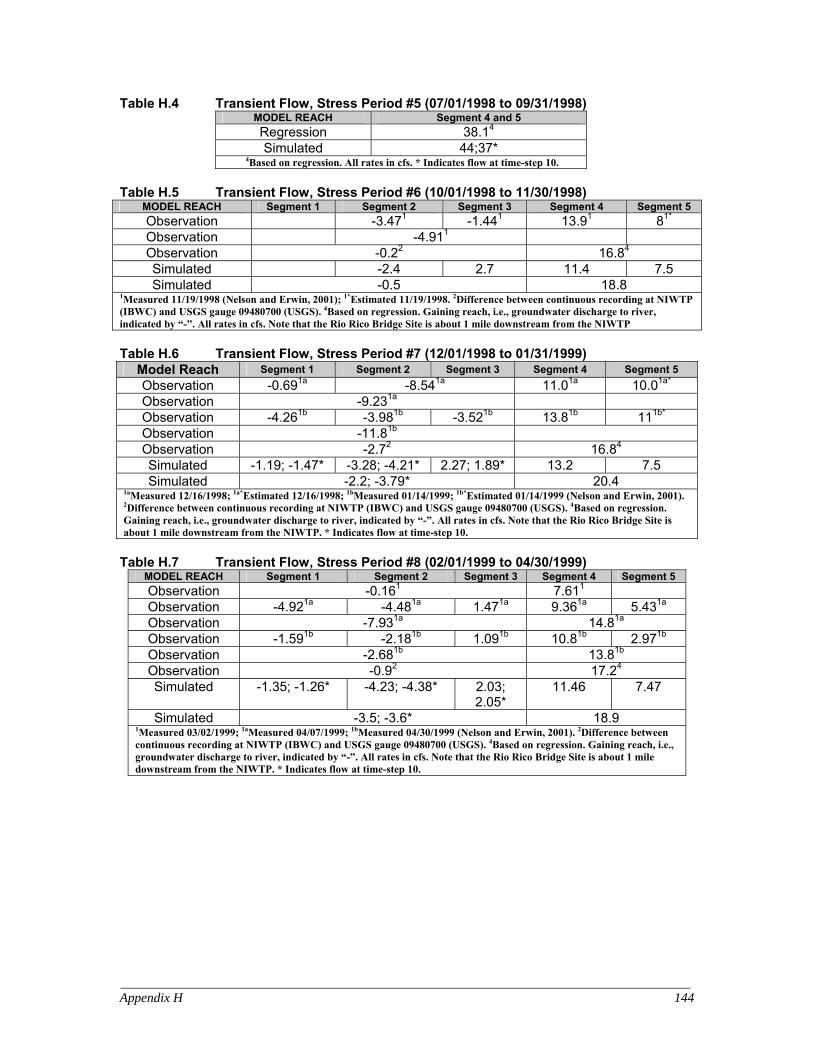
_____________________________________________________________________________________ Appendix H 144
Table H.4 Transient Flow, Stress Period #5 (07/01/1998 to 09/31/1998) MODEL REACH Segment 4 and 5 Regression 38.14 Simulated 44;37*
4Based on regression. All rates in cfs. * Indicates flow at time-step 10. Table H.5 Transient Flow, Stress Period #6 (10/01/1998 to 11/30/1998)
MODEL REACH Segment 1 Segment 2 Segment 3 Segment 4 Segment 5 Observation -3.471 -1.441 13.91 81* Observation -4.911 Observation -0.22 16.84 Simulated -2.4 2.7 11.4 7.5 Simulated -0.5 18.8
1Measured 11/19/1998 (Nelson and Erwin, 2001); 1*Estimated 11/19/1998. 2Difference between continuous recording at NIWTP (IBWC) and USGS gauge 09480700 (USGS). 4Based on regression. Gaining reach, i.e., groundwater discharge to river, indicated by “-”. All rates in cfs. Note that the Rio Rico Bridge Site is about 1 mile downstream from the NIWTP Table H.6 Transient Flow, Stress Period #7 (12/01/1998 to 01/31/1999)
Model Reach Segment 1 Segment 2 Segment 3 Segment 4 Segment 5 Observation -0.691a -8.541a 11.01a 10.01a* Observation -9.231a Observation -4.261b -3.981b -3.521b 13.81b 111b* Observation -11.81b Observation -2.72 16.84 Simulated -1.19; -1.47* -3.28; -4.21* 2.27; 1.89* 13.2 7.5 Simulated -2.2; -3.79* 20.4
1aMeasured 12/16/1998; 1a*Estimated 12/16/1998; 1bMeasured 01/14/1999; 1b*Estimated 01/14/1999 (Nelson and Erwin, 2001). 2Difference between continuous recording at NIWTP (IBWC) and USGS gauge 09480700 (USGS). 4Based on regression. Gaining reach, i.e., groundwater discharge to river, indicated by “-”. All rates in cfs. Note that the Rio Rico Bridge Site is about 1 mile downstream from the NIWTP. * Indicates flow at time-step 10.
Table H.7 Transient Flow, Stress Period #8 (02/01/1999 to 04/30/1999)
MODEL REACH Segment 1 Segment 2 Segment 3 Segment 4 Segment 5 Observation -0.161 7.611 Observation -4.921a -4.481a 1.471a 9.361a 5.431a Observation -7.931a 14.81a Observation -1.591b -2.181b 1.091b 10.81b 2.971b Observation -2.681b 13.81b Observation -0.92 17.24 Simulated -1.35; -1.26* -4.23; -4.38* 2.03;
2.05* 11.46 7.47
Simulated -3.5; -3.6* 18.9 1Measured 03/02/1999; 1aMeasured 04/07/1999; 1bMeasured 04/30/1999 (Nelson and Erwin, 2001). 2Difference between continuous recording at NIWTP (IBWC) and USGS gauge 09480700 (USGS). 4Based on regression. Gaining reach, i.e., groundwater discharge to river, indicated by “-”. All rates in cfs. Note that the Rio Rico Bridge Site is about 1 mile downstream from the NIWTP. * Indicates flow at time-step 10.

_____________________________________________________________________________________ Appendix H 145
Table H.8 Transient Flow, Stress Period #9 (05/01/1999 to 06/30/1999) MODEL REACH Segment 1 Segment 2 Segment 3 Segment 4 Segment 5 Observation -3.01a 5.251a 8.01a Observation 2.251a Observation 3.831b -2.381b 4.721b Observation 6.171b Observation 8.92 Simulated 0.34; 1.93* -1.77; 1.54* 4.1; 5.82* 11.7; 5.1* 0.0; 0* Simulated 2.7; 9.3* 12.6; 5.1*
1aMeasured 05/26/1999; 1bMeasured 06/24/1999 (Nelson and Erwin, 2001). 2Difference between continuous recording at NIWTP (IBWC) and USGS gauge 09480700 (USGS). 4Based on regression. Gaining reach, i.e., groundwater discharge to river, indicated by “-”. All rates in cfs. Note that the Rio Rico Bridge Site is about 1 mile downstream from the NIWTP. * Indicates flow at time-step 10.
Table H.9 Transient Flow, Stress Period #10 (07/01/1999 to 09/30/1999)
MODEL REACH Segment 4 and 5 Regression 47.64 Simulated 58
4Based on regression. All rates in cfs. * Indicates flow at time-step 10. Table H.10 Transient Flow, Stress Period #11 (10/01/1999 to 11/30/1999)
MODEL REACH Segment 1 Segment 2 Segment 3 Segment 4 Segment 5 Observation 0.531a -1.11a -2.01a 8.341a 11.01a Observation -2.571a 19.31a Observation -4.02 24.44 Simulated -1.0;-1.1* -2.2; -
2.5* 2.3;2.5* 10.5 7.5
Simulated -1.0; -1.11* 18 1aMeasured 10/27/1999 (Nelson and Erwin, 2001). 2Difference between continuous recording at NIWTP (IBWC) and USGS gauge 09480700 (USGS). 4Based on regression. Gaining reach, i.e., groundwater discharge to river, indicated by “-”. All rates in cfs. Note that the Rio Rico Bridge Site is about 1 mile downstream from the NIWTP. * Indicates flow at time-step 10.
Table H.11 Transient Flow, Stress Period #12 (12/01/1999 to 01/31/2000)
MODEL REACH Segment 1 Segment 2 Segment 3 Segment 4 Segment 5 Observation 01a -6.01a 01a 8.01a 3.01a Observation -6.01a 11.01a Observation -4.82 194 Simulated -1.35; -1.6* -3.1; -4.1* 2.2; 1.9* 11.3 7.4 Simulated -2.25; -3.81* 18.7
1aMeasured 01/26/2000 (Nelson and Erwin, 2001). 2Difference between continuous recording at NIWTP (IBWC) and USGS gauge 09480700 (USGS). 4Based on regression. Gaining reach, i.e., groundwater discharge to river, indicated by “-”. All rates in cfs. Note that the Rio Rico Bridge Site is about 1 mile downstream from the NIWTP. * Indicates flow at time-step 10.

_____________________________________________________________________________________ Appendix H 146
Table H.12 Transient Flow, Stress Period #13 (02/01/2000 to 04/30/2000) MODEL REACH Segment 1 Segment 2 Segment 3 Segment 4 Segment 5 Observation -0.71a -3.941a -0.121a 8.651a Observation -4.761a Observation -1.591b -1.321b 1.491b 11.11b Observation -1.421b Observation -2.42 20.74 Simulated -1.5; -1.4* -4.1; -4.2* 2.0; 2.0* 11.4 7.4 Simulated -3.6; -3.6* 18.8
1aMeasured 03/29/2000; 1bMeasured 04/26/2000 (Nelson and Erwin, 2001). 2Difference between continuous recording at NIWTP (IBWC) and USGS gauge 09480700 (USGS). 4Based on regression. Gaining reach, i.e., groundwater discharge to river, indicated by “-”. All rates in cfs. Note that the Rio Rico Bridge Site is about 1 mile downstream from the NIWTP. * Indicates flow at time-step 10.
Table H.13 Transient Flow, Stress Period #14 (05/01/2000 to 06/30/2000)
MODEL REACH Segment 1 Segment 2 Segment 3 Segment 4 Segment 5 Observation 1.421 -0.751 1.911 8.51 Observation 2.581 Observation 1.571a -1.691a 3.891a Observation 3.771a Observation 8.72a 14.94 Simulated -0.16; 1.8* -1.7; 1.7* 4.3; 6.0* 13.1; 14.6* 7.5; 4.0* Simulated 0.61; 9.5* 20.6; 18.5*
1Measured 05/17/2000; 1aMeasured 06/14/2000 (Nelson and Erwin, 2001). 2aDifference between continuous recording at NIWTP (IBWC) and USGS gauge 09480700 (USGS); removed run-off components - includes only baseflow. 4Based on regression. Gaining reach, i.e., groundwater discharge to river, indicated by “-”. All rates in cfs. Note that the Rio Rico Bridge Site is about 1 mile downstream from the NIWTP. * Indicates flow at time-step 10.
Table H.14 Transient Flow, Stress Period #15 (07/01/2000 to 09/30/2000)
MODEL REACH Segment 4 and 5 Regression 20.84 Simulated 18
4Based on regression. All rates in cfs. Table H.15 Transient Flow, Stress Period #16 (10/1/2000 to 11/30/2000)
MODEL REACH Segment 4 and 5 Regression 3534 Simulated 173; 87*
4Based on regression; high flow (observed data) does not fit regression-based estimate. All rates in cfs. * Indicates flow at time-step 10.
Table H.16 Transient Flow, Stress Period #17 (12/1/2000 to 1/31/2001)
MODEL REACH Segment 4 and 5 Regression 664 Simulated 52
4Based on regression. All rates in cfs.

_____________________________________________________________________________________ Appendix H 147
Table H.17 Transient Flow, Stress Period #18 (2/1/2001 to 4/30/2001)
MODEL REACH Segment 1 Segment 2 Segment 3 Segment 4 Segment 5 Observation -161a** 9.91a 12.91a Observation 22.81a Observation -3.851b 12.31b 12.31b Observation 24.61b Regression 444 Simulated 2.68 19 19 Simulated -2.9 38
1aMeasured 02/12/2001 [**contains both overland surface water flow components, as well as, groundwater discharge components]; 1bMeasured 03/29/2001 (Nelson and Erwin, 2001). 4Based on regression. Gaining reach, i.e., groundwater discharge to river, indicated by “-”. All rates in cfs. Note that the Rio Rico Bridge Site is about 1 mile downstream from the NIWTP.
Table H.18 Transient Flow, Stress Period #19 (05/01/2001 to 06/30/2001)
MODEL REACH Segment 1 Segment 2 Segment 3 Segment 4 and 5 Observation 4.21a -1.01a Regression Flow at Tubac effected by runoff 164 Simulated 6.3; 13.4* -1.0; 2.8* 3.4; 6.2* 21; 23* Simulated 8.7; 22*
1aMeasured 06/27/2001 (Nelson and Erwin, 2001). 4Based on regression. Gaining reach, i.e., groundwater discharge to river, indicated by “-”. All rates in cfs. Note that the Rio Rico Bridge Site is about 1 mile downstream from the NIWTP. * Indicates flow at time-step 10.
Table H.19 Transient Flow Stress Period #20 (07/01/2001 to 09/30/2001)
MODEL REACH Segment 4 and 5 Regression 154 Simulated 27
4Based on regression. All rates in cfs. Table H.20 Transient Flow, Stress Period #21 (10/01/2001 to 11/30/2001)
MODEL REACH Segment 1 - 3 Segment 4 and 5 Observation 5.72 16.84 Simulated 3.2; 0.93* 18.5
2Difference between continuous recording at NIWTP (IBWC) and USGS gauge 09480700 (USGS). 4Based on regression. Gaining reach, i.e., groundwater discharge to river, indicated by “-”. All rates in cfs. Note that the Rio Rico Bridge Site is about 1 mile downstream from the NIWTP. * Indicates flow at time-step 10.
Table H.21 Transient Flow, Stress Period #22 (12/01/2001 to 01/31/2002)
MODEL REACH Segment 1 -3 Segment 4 and 5 Observation/Regression -3.52 234
Simulated -0.65; -2.9* 18 2Difference between continuous recording at NIWTP (IBWC) and USGS gauge 09480700 (USGS). 4Based on regression. Gaining reach, i.e., groundwater discharge to river, indicated by “-”. All rates in cfs. Note that the Rio Rico Bridge Site is about 1 mile downstream from the NIWTP. * Indicates flow at time-step 10.
Table H.22 Transient Flow, Stress Period #23 (02/01/2002 to 04/30/2002)
MODEL REACH Segment 1 and 2 Segment 3 Segment 4 and 5 Observation -3.41 17.51
Observation/Regression -0.72 184 Simulated -1.5 Simulated -3.0; -3.33* 18.2
1Measured 02/27/2002, ADWR_2002. 2Difference between continuous recording at NIWTP (IBWC) and USGS gauge 09480700 (USGS). 4Based on regression. Gaining reach, i.e., groundwater discharge to river, indicated by “-”. All rates in cfs. Note that the Rio Rico Bridge Site is about 1 mile downstream from the NIWTP. * Indicates flow at time-step 10.
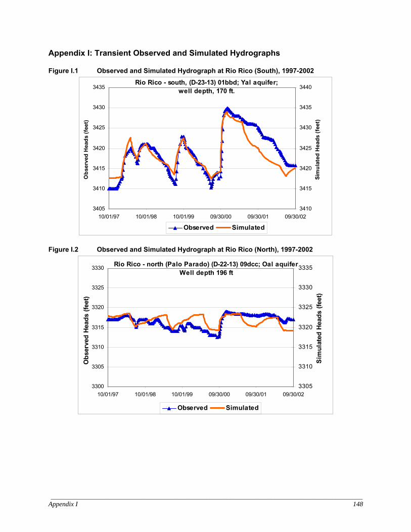
____________________________________________________________________________________________ Appendix I 148
Appendix I: Transient Observed and Simulated Hydrographs Figure I.1 Observed and Simulated Hydrograph at Rio Rico (South), 1997-2002
Rio Rico - south, (D-23-13) 01bbd; Yal aquifer; well depth, 170 ft.
3405
3410
3415
3420
3425
3430
3435
10/01/97 10/01/98 10/01/99 09/30/00 09/30/01 09/30/02
Obs
erve
d H
eads
(fee
t)
3410
3415
3420
3425
3430
3435
3440
Sim
ulat
ed H
eads
(fee
t)
Observed Simulated
Figure I.2 Observed and Simulated Hydrograph at Rio Rico (North), 1997-2002
Rio Rico - north (Palo Parado) (D-22-13) 09dcc; Oal aquiferWell depth 196 ft
3300
3305
3310
3315
3320
3325
3330
10/01/97 10/01/98 10/01/99 09/30/00 09/30/01 09/30/02
Obs
erve
d H
eads
(fee
t)
3305
3310
3315
3320
3325
3330
3335
Sim
ulat
ed H
eads
(fee
t)
Observed Simulated

____________________________________________________________________________________________ Appendix I 149
Figure I.3 Observed and Simulated Hydrograph at Tumacacori, 1997-2002 Tumacacori (D-21-13) 30dca; Oal aquifer. Well depth 150 ft
3220
3225
3230
3235
3240
3245
3250
10/01/97 10/01/98 10/01/99 09/30/00 09/30/01 09/30/02
Obs
erve
d H
eads
(fee
t)
3222
3227
3232
3237
3242
3247
3252
Sim
ulat
ed H
eads
(fee
t)
Observed Simulated
Figure I.4 Observed and Simulated Hydrograph at Tubac, 1997-2002
Tubac (D-21-13) 05ccb; Yal aquifer. Well depth 32 ft.
3140
3145
3150
3155
3160
3165
3170
10/01/97 10/01/98 10/01/99 09/30/00 09/30/01 09/30/02
Obs
erve
d He
ads
(feet
)
3145
3150
3155
3160
3165
3170
3175
Sim
ulat
ed H
eads
(fee
t)
Observed Simulated

____________________________________________________________________________________________ Appendix I 150
Figure I.5 Observed and Simulated Hydrograph at Chavez Siding, 1997-2002 Chavez Siding (D-20-13) 32bcc; Yal & Oal aquifers.
Well depth 185 ft.
3110
3115
3120
3125
3130
3135
3140
10/01/97 10/01/98 10/01/99 09/30/00 09/30/01 09/30/02
Obs
erve
d H
eads
(fee
t)
3120
3125
3130
3135
3140
3145
3150
Sim
ulat
ed H
eads
(Fee
t)
Observed Simulated
Figure I.6 Observed and Simulated Hydrograph at Amado, 1997-2002
Amado (D-20-13) 07acd; Yal aquifer. Well depth 123 ft.
3035
3040
3045
3050
3055
3060
3065
10/01/97 10/01/98 10/01/99 09/30/00 09/30/01 09/30/02
Hea
ds (f
t)
Observed Simulated

____________________________________________________________________________________________ Appendix I 151
Figure I.7 Observed and Simulated Hydrograph at Arivaca Junction, 1997-2002 Arivaca Junction (D-19-13) 31abd; Yal & Oal aquifers
Well depth 88 ft
2970
2975
2980
2985
2990
2995
3000
10/01/97 10/01/98 10/01/99 09/30/00 09/30/01 09/30/02
Obs
erve
d H
eads
(fee
t)
2978
2983
2988
2993
2998
3003
3008
Sim
ulat
ed H
eads
(Fee
t)
Observed Simulated
Figure I.8 Observed and Simulated Hydrograph at Elephant Head Bridge, 1997-2002
Elephant Head (D-19-13) 29bcc; Oal aquiferWell depth 500 ft.
2955
2960
2965
2970
2975
2980
2985
10/01/97 10/01/98 10/01/99 09/30/00 09/30/01 09/30/02
Obs
erve
d H
eads
(fee
t)
2958
2963
2968
2973
2978
2983
2988
Sim
ulat
ed H
eads
(fee
t)
Observed Simulated

____________________________________________________________________________________________ Appendix I 152
Figure I.9 Observed and Simulated Hydrograph at Rio Rico (South), 1949-1959
Rio Rico: (D-22-13) 35dcd; Yal aquifer. Well depth 90 ft.
3360
3370
3380
3390
3400
3410
3420
09/30/49 09/30/51 09/29/53 09/29/55 09/28/57 09/28/59
Obs
erve
d H
eads
(fee
t)
3355
3365
3375
3385
3395
3405
3415
Sim
ulat
ed H
eads
(fee
t)
Observed Simulated
Figure I.10 Observed and Simulated Hydrograph at Rio Rico (North), 1949-1959
Rio Rico - North (D-22-13) 09daa; Yal aquifer. Well depth 75 ft.
3260
3270
3280
3290
3300
3310
3320
09/30/49 09/30/51 09/29/53 09/29/55 09/28/57 09/28/59
Obs
erve
d He
ads
(feet
)
3275
3285
3295
3305
3315
3325
3335
Sim
ulat
ed H
eads
(fee
t)
Observed Simulated

____________________________________________________________________________________________ Appendix I 153
Figure I.11 Observed and Simulated Hydrograph at Tubac, 1949-1959 Tubac: (D-21-13) 18 dda; Yal aquifer. Well depth 30 ft.
3160
3170
3180
3190
3200
3210
3220
09/30/49 09/30/51 09/29/53 09/29/55 09/28/57 09/28/59
Obs
erve
d H
eads
(fee
t)
3165
3175
3185
3195
3205
3215
3225
Sim
ulat
ed H
eads
(fee
t)
Observed Simulated
Figure I.12 Observed and Simulated Hydrograph at Amado, 1949-1959
Amado: (D-20-13) 07cdc; Yal/Oal aquifer.Well depth 183 ft.
3010
3020
3030
3040
3050
3060
3070
09/30/49 09/30/51 09/29/53 09/29/55 09/28/57 09/28/59
Obs
erve
d H
eads
(fee
t)
3005
3015
3025
3035
3045
3055
3065
Sim
ulat
ed H
eads
(fee
t)
Observed Simulated

____________________________________________________________________________________________ Appendix I 154
Figure I.13 Observed and Simulated Hydrograph at Arivaca Junction, 1949-1959 Arivaca Junction: (D-19-13) 31dcc. Yal/Oal aquifer.
Well depth 175 ft.
2970
2980
2990
3000
3010
3020
3030
09/30/49 09/30/51 09/29/53 09/29/55 09/28/57 09/28/59
Obs
erve
d H
eads
(fee
t)
2955
2965
2975
2985
2995
3005
3015
Sim
ulat
ed H
eads
(Fee
t)
Observed Simulated