Arithmetic properties of Schwarz maps

Hironori Shiga, Yoshio Suzuki and Jurgen Wolfart

Version September 24, 2008

The subject of this article belongs to the general question Under which condition(s) suit-ably normalized transcendental functions take algebraic values at algebraic arguments? Al-ready the classical examples of Weierstrass’ result concerning the exponential functionand Theodor Schneider’s result about the elliptic modular function show that argumentsand values in these cases are of particular arithmetical interest. Here we try to answerthis question for the case of Schwarz maps belonging to Appell–Lauricella hypergeometricfunctions FD in two and more variables, generalizing our results in [SW2] about Schwarztriangle functions, i.e. for the classical Gauss hypergeometric functions in one variable.

The first section contains the necessary basic notations, conventions and the known ma-chineries from hypergeometric functions, transcendence and abelian varieties. The secondpresents the main result about necessary and sufficient conditions for algebraic and non–algebraic values of Schwarz maps. These are valid only in some Zariski open subset ofthe domain of definition, and the last section shows by giving some examples that thisrestriction is quite natural.

1 Basics

1.1 Appell-Lauricella functions

With the Pochhammer symbol (a, 0) := 1 , (a, n) := a(a+ 1) · . . . · (a+n− 1) for complexa and positive integers n the Appell–Lauricella functions F1 in the N complex variablesx2, x3, . . . , xN+1 with parameters a, b2, . . . , bN+1 and c ∈ C , c 6= 0,−1,−2, . . . — forN > 2 often denoted FD in the literature — can be defined by the series

F1(a, b2, . . . , bN+1, c;x2, . . . , xN+1) :=∑

n2

. . .∑

nN+1

(a,∑

j nj)∏

j(bj, nj)

(c,∑

j nj)∏

j(1, nj)

N+1∏

j=2

xnj

j , (1)

each nj running from 0 to ∞ . The series converges if all |xj| < 1 . We will use almosteverywhere its integral representation

1

B(1 − µ1, 1 − µN+2)

∫u−µ0(u− 1)−µ1

∏

j

(u− xj)−µjdu , (2)

1

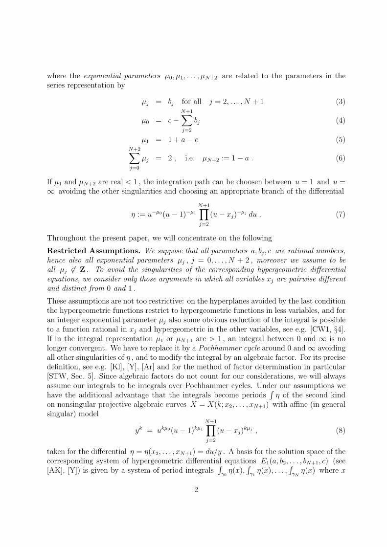
where the exponential parameters µ0, µ1, . . . , µN+2 are related to the parameters in theseries representation by

µj = bj for all j = 2, . . . , N + 1 (3)

µ0 = c−N+1∑

j=2

bj (4)

µ1 = 1 + a− c (5)N+2∑

j=0

µj = 2 , i.e. µN+2 := 1 − a . (6)

If µ1 and µN+2 are real < 1 , the integration path can be choosen between u = 1 and u =∞ avoiding the other singularities and choosing an appropriate branch of the differential

η := u−µ0(u− 1)−µ1

N+1∏

j=2

(u− xj)−µj du . (7)

Throughout the present paper, we will concentrate on the following

Restricted Assumptions. We suppose that all parameters a, bj, c are rational numbers,hence also all exponential parameters µj , j = 0, . . . , N + 2 , moreover we assume to beall µj 6∈ Z . To avoid the singularities of the corresponding hypergeometric differentialequations, we consider only those arguments in which all variables xj are pairwise differentand distinct from 0 and 1 .

These assumptions are not too restrictive: on the hyperplanes avoided by the last conditionthe hypergeometric functions restrict to hypergeometric functions in less variables, and foran integer exponential parameter µj also some obvious reduction of the integral is possibleto a function rational in xj and hypergeometric in the other variables, see e.g. [CW1, §4].If in the integral representation µ1 or µN+1 are > 1 , an integral between 0 and ∞ is nolonger convergent. We have to replace it by a Pochhammer cycle around 0 and ∞ avoidingall other singularities of η , and to modify the integral by an algebraic factor. For its precisedefinition, see e.g. [Kl], [Y], [Ar] and for the method of factor determination in particular[STW, Sec. 5]. Since algebraic factors do not count for our considerations, we will alwaysassume our integrals to be integrals over Pochhammer cycles. Under our assumptions wehave the additional advantage that the integrals become periods

∫η of the second kind

on nonsingular projective algebraic curves X = X(k;x2, . . . , xN+1) with affine (in generalsingular) model

yk = ukµ0(u− 1)kµ1

N+1∏

j=2

(u− xj)kµj , (8)

taken for the differential η = η(x2, . . . , xN+1) = du/y . A basis for the solution space of thecorresponding system of hypergeometric differential equations E1(a, b2, . . . , bN+1, c) (see[AK], [Y]) is given by a system of period integrals

∫γ0η(x),

∫γ1η(x), . . . ,

∫γNη(x) where x

2

denotes the n–tuple (x2, . . . , xN+1) of variables and the integration paths γi are suitablychosen Pochhammer cycles in the u–plane, each of them going around a pair of singularitiesu = 0, 1, x2, . . . , xN+1,∞ .

1.2 Jacobians and Prym varieties

Following the method of [CW2, Sec. 3] for N = 2 and [SW1, §5] we keep the right handside of equation (8) and replace the left hand side with yd where d denotes a proper divisorof k , obtaining a smooth complex projective algebraic curve X(d, x) and an obviousepimorphism X(k, x) → X(d, x) . It induces an epimorphism of Jacobians

md : JacX(k, x) → JacX(d, x) .

Let the Prym variety T (k, x) be the connected component of 0 in the intersection⋂

Kermd ,d running over all proper divisors of k . Then T (k, x) is an abelian variety of complex di-mension N+1

2ϕ(k) where ϕ denotes Euler’s function. As in the case N = 1 (see [Wo]

or [SW2, Sec. 1.2]) it has generalized complex multiplication by a cyclotomic field, moreprecisely we have

Q(ζk) ⊆ End0T (k, x) := Q ⊗Z EndT (k, x)

induced by the automorphism of the curve X(k, x) described on its singular model by

σ : (u, y) 7→ (u, ζ−1k y) , ζk = e

2πik .

For a more precise description of the complex analytic family of abelian varieties con-taining T (k, x) we need also its type. It is determined as follows. On the vector spaceH0(T (k, x),Ω) of first kind differentials on T = T (k, x) we have an induced action ofQ(ζk) splitting the vector space in eigenspaces Vσ = Vn, n ∈ (Z/kZ)∗ , of differentials ωwith the property

ω σ = ζnk · ω .

According to Chevalley and Weil [ChWe] the dimensions of the eigenspaces can be calcu-lated as

rn := dimVn = −1 +N+2∑

j=0

〈nµj〉 (9)

where 〈α〉 := α− [α] denotes the fractional part of α . It is easy to see that

rn + r−n = N + 1

for all n coprime to k . We will always identify the differentials of the first kind with certainholomorphic differentials on the curve X(k, x) where we can study the action of σ in anobvious way. If e.g. all exponential parameters satisfy µj < 1 , the differential η = du

y

3

in equation (7) is in this identification an element of V1 . Now the type of T (k, x) can beintroduced as the formal sum

∑

σ∈GalQ(ζk)/Q

(dimVσ) · σ

or in simplified version as the ϕ(k)–tuple (rn | n ∈ (Z/kZ)∗)) .

We should remark by the way that we use also two further and similar identifications of(co)homology groups. First, by the natural action of the endomorphism algebra we canconsider the homology group H1(T (k, x),Z) of rank (N+1)ϕ(k) as being a rank (N+1)–module over Z[ζk] whose cycles all come from cycles on X(k, x) . In particular, we canconsider the Pochhammer cycles γ0, γ1, . . . , γN as generators of the Q(ζk)–vector spaceH1(T (k, x),Q) := Q ⊗Z H

1(T (k, x),Z) .Second, we identify the space H1

DR(T (k, x)) of second kind differentials on our Prymvariety with a subspace of the second kind differentials on the curve. As H0(T (k, x),Ω) ,it splits in Q(ζk)–eigenspaces Wn ⊇ Vn , all of dimension dimWn = N + 1 . This can beshown either by complex algebraic geometry ([GH] or [Be, §4, Remarque 1]) or as anotherversion of a well known principle concerning associate functions to be explained now.

1.3 Associate hypergeometric functions

Hypergeometric functions F1(a, b2, . . . , bN+1, c;x2, . . . , xN+1) are called associate if theirparameter (N + 2)–tuples (a, b2, . . . , bN+1, c) are congruent mod ZN+2 , in other words ifall their exponential parameters µj differ by integers only (always under the condition that∑µj = 2 is preserved, of course). If we write their differential in a slightly more general

way than (7) as η = r(u)du/yn ∈ Wn with a rational function r(u) = um0(u−1)m1∏

(u−xj)

mj , all mj ∈ Z , then a differential for an associate hypergeometric function differs fromthat one by another choice of the rational function r only, but obviously remaining in Wn .So if we keep the Pochhammer cycle γi on the curve fixed — identified as above with agenerator of H1(T (k, x),Q) — the periods

∫γiη(x) , η ∈ Wn , generate as functions of x

a complex vector space of associate hypergeometric functions. Now it is known that thisvector space has dimension N +1 over the space of rational functions in x [Y]. Recall thatall parameters are rational, so all normalizing Beta values for associate hypergeometricfunctions differ by rational factors only such that this dimension result may be formulatedfor the differentials as follows.

Lemma 1.1. Under our assumptions, for all fixed n coprime to k , any N + 2

different differentials of type

η(x) =um0(u− 1)m1

∏(u− xj)

mj

yndu ∈ Wn , all mj ∈ Z , (10)

satisfy a nontrivial linear relation modulo exact differentials with coefficients in the poly-nomial ring Q[x2, . . . , xN+1] .

4

We will use this fact also in another way, concentrating on the behaviour in special fixedarguments x . Henceforth we will call these differentials of type (10) in a common eigenspaceWn associate differentials.

Lemma 1.2. For all n coprime to k and any N+1 different associate differentials ην(x) ∈Wn ⊂ H1

DR(T (k, x)) there is a Zariski dense subset Z ⊂ CN of arguments x in which theην(x) form a basis of Wn .

To the complementary set CN\Z we always add the hyperplanes xj = 0 , 1 and xi = xj

forbidden by our restrictive assumptions.

1.4 Schwarz maps

For any η(x) of type (10) and any such Zariski dense subset Z as in Lemma 1.2 we definethe Schwarz map as the function

Dη : Z → PN(C) : x 7→(∫

γ0

η(x) : . . . :

∫

γN

η(x)

).

(Since the components form a basis of a system of linear differential equations and since weconsider regular points only, these components cannot all vanish.) As always with Schwarzmaps, this is a priori only locally well defined since analytic continuation in Z is not globallypossible without deforming the Pochhammer cycles. Since Z is not simply connected,Dη is multivalued, and this multivaluedness can be described by the (linear) action ofthe homotopy group of Z either on the solution space of the system of hypergeometricdifferential equations or on the homology H1(T (k, x),Z) , see [Y]. The components ofthe image could have given also in terms of normalized basis solutions of a hypergeometricdifferential equation system of Appell–Lauricella type D since the normalizing Beta factorsare all the same up to rational factors, hence do not count if we work with projectivecoordinates, at least up to projective linear transformations defined over Q .

The central question is now: suppose the argument x = τ is an algebraic point of Z ,i.e. has all its coordinates xj = τj ∈ Q . Under which conditions Dη(τ) is an algebraicpoint, i.e. is in PN(Q) , in other words has coordinates which are Q–multiples of eachother? Note first that the curve X(k, τ) is defined over Q as well as its Jacobian and thePrym variety T (k, τ) . Moreover, all differentials in (7) or (10) are defined over Q , andtherefore we will consider all cohomology groups H0(T (k, τ),Ω) , H1

DR(T (k, τ)) as vectorspaces over Q . The question is well posed since under the monodromy action the baseγ0, . . . , γN changes only under a matrix in GLN+1(Z[ζk]) and the differential η(τ) remainsunchanged, so the algebraicity of the value Dη(τ) remains unchanged.

5

1.5 Monodromy groups and modular groups

Finally we should mention that all abelian varieties T with common dimension and po-larization, with generalized CM by Q(ζk) and of the same CM type can be parametrizedby a complex symmetric domain D . According to Siegel [Si] and Shimura [Sh] dimD =∑

R rnr−n where the summation runs over a system R of representatives of (Z/kZ)∗ mod±1 , in other words over a system of representations of the CM field modulo complexconjugation. The symmetric domain is a product of spaces Hrn,r−n

of rn × r−n–matricesz with the property that 1 − ztz is positive hermitian. Two points on D correspond toisomorphic abelian varieties if and only if they lie in the same orbit of the modular group forthis family. Since the monodromy group of our hypergeometric function does not changethe curve X(k, x) nor its Jacobian or the Prym variety, we can consider it as a subgroup ofthe modular group. Several special cases have to be mentioned (recall rn + r−n = N + 1 ).

• In the case that rn or r−n = 0 the matrix space degenerates to one point, so the factorHrn,r−n

of D can be omitted. This may even occur for all n . In that case, thereis only one isogeny class of abelian varieties of this CM type, and this is necessarilyone of complex multiplication type in the narrow sense ([ShT] or [La, Ch 1]), i.e.isogenous to a product of simple abelian varieties A whose endomorphism algebraEnd0A is a (CM) field of degree 2 dimA . In our construction, this occurs preciselyif the hypergeometric functions are algebraic functions, and these cases occur if andonly if there is an x such that T (k, x) is isogenous to a power of a simple abelianvariety with CM. For the classical Schwarz case N = 1 see [SW2, Prop. 2.8], andin the Appell–Lauricalla cases N > 1 these possibilities are discussed in [Sa] and[CW1]. For N > 3 there are no such cases.

• In the one variable case (N = 1 ) D is isomorphic to a product of upper half planes.This case is treated in [SW2].

• In the case N > 1 all nontrivial factors of D are isomorphic to complex N–balls ifrn or r−n = 1 . This is necessarily the case for N = 2 .

• If in these cases D consists of only one factor, i.e. if rn = 1 for precisely one ncoprime to k , the Prym varieties T (k, x) form a Zariski dense subset of all abelianvarieties of its CM type, and the monodromy group is commensurable to the modulargroup. In other words, it is arithmetically defined.

• If in these cases moreover η = ω is a generator of the one–dimensional eigenspaceVn ⊂ H0(T (k, x),Ω) , the Schwarz map Dω has — up to linear transformations —its images in D and is a converse to a mapping composed by suitably normalizedautomorphic functions for an arithmetic group commensurable to the modular groupmentioned above.

• Therefore, in these cases our central question is answered by the Main Theorem and

6

its Corollary in [SW1]: for an algebraic τ we have an algebraic value Dω(τ) if andonly if the Prym variety T (k, τ) is of CM type.

For the last statement, [SW1, Cor. 6] gives a slight generalization to a more complicatedsituation involving N + 1 differentials of the first kind, but Thms. 3.4 and 3.5 of [SW2]show that even in the one variable case, such a neat result cannot be expected for Schwarzmaps coming from differentials of the second kind. In Section 2 we will try to extend thisobservation to N > 1 .

1.6 Period relations and transcendence

The main instrument to get transcendence results in this context is Wustholz’ analyticsubgroup theorem [Wu]. The proof for its consequence to period relations is worked outby Paula Cohen in the appendix of [STW]. We state its content as

Lemma 1.3. Let A be an abelian variety isogenous over Q to the direct product Ak11 ×

. . . × AkN

N of simple, pairwise non-isogenous abelian varieties Aν defined over Q, with Aν

of dimension nν , ν = 1, . . . , N . Then the Q–vector space VA generated by 1, 2πi togetherwith all periods of differentials, defined over Q , of the first and the second kind on A , hasdimension

dimQ VA = 2 + 4N∑

ν=1

n2ν

dimQ End0Aν

.

This Lemma governs all Q–linear relations beween periods, but it does not say anythingabout possible nonlinear relations. Riemann’s period relations give examples of those.Since we will need them in the last section, we state them here as

Lemma 1.4. (Riemann bilinear relations)Let X be a compact Riemann surface of genus g, and let A1, ..., Ag, B1, ..., Bg be a canon-ical homology basis of X with AiBj = δij, AiAj = BiBj = 0 (1 ≤ i, j ≤ g). For aholomorphic differential ω and a meromorphic differential η with poles sλ we have

g∑

i=1

(

∫

Ai

ω

∫

Bi

η −∫

Bi

ω

∫

Ai

η) = 2π√−1∑

λ

Ressλ(η)

∫ sλ

s0

ω.

2 Algebraic values of Schwarz maps

2.1 A necessary condition

Theorem 2.1. Let τ be an algebraic point of CN , all components pairwise different and6= 0 , 1 . Under the restricted assumptions and for the differentials η ∈ Wn of type (10)

7

suppose that the Schwarz map Dη takes an algebraic value Dη(τ) ∈ PN(Q) . Then thePrym variety T (k, τ) has a simple CM factor S with complex multiplication by a CM fieldK such that η is induced by a K–eigendifferential on S .

Proof. For a first kind differential η = ω this is a consequence of [SW1, Cor. 1]: sinceγ0, . . . , γN form a basis of the homology of T (k, τ) as Q(ζk)–vector space and η is aneigendifferential for the action of this field, all periods

∫γη are algebraic multiples of each

other, so the hypotheses of [SW1, Cor. 1] are satisfied.For the second kind differentials η not belonging to H0(T (k, τ),Ω) , we can deduce theexistence of a corresponding first kind differential ω with the same property from this oneusing the fact that representations of endomorphisms on the period lattice and on thequasiperiod lattice are complex conjugate to each other, or by passing to the dual abelianvariety, see [Be, §4, Remarques 1 et 2]. Therefore we can apply the argument of the firstpart again.

In the case N = 1 there is a much more precise statement due to the fact that thecomplement of a CM factor of T (k, τ) is necessarily of CM type as well [SW2, Prop. 2.4],hence T (k, τ) is itself of CM type. For N > 1 , any factor A of T (k, τ) with CM by Q(ζk)has — up to isogeny — still a complement B with generalized CM by Q(ζk) [Be, Thm 1],but since dimB > 1

2ϕ(k) , it is not necessarily of CM type in the narrow sense.

2.2 Periods on Pryms with CM factors

A closer look to the proof of Theorem 2.1 and its background in transcendence theoryof periods — see [CW1] — shows that Dη can only be algebraic if (up to isogeny) thereis a decomposition T (k, τ) = A ⊕ B in two abelian varieties such that A has complexmultiplication by Q(ζk) and η belongs to the first factor in the corresponding decomposition

H1DR(T (k, τ) = H1

DR(A) ⊕H1DR(B) .

This is necessarily the case if the hypergeometric functions are algebraic (see the preceedingsection) since then T (k, x) is isogenous to AN+1 , and this decomposition can be choosenin many ways such that we can suppose that η belongs to the factor A . Moreover we canthen suppose η ∈ H1

DR(S) , S a simple factor of A with complex multiplication by a CMfield K ⊆ Q(ζk) such that 2 dimS = [K : Q] and η is a K–eigendifferential. In that casethe vector space Πη ⊂ C generated over Q by all periods of η has dimension 1 , see thearguments of [SW2, Prop. 2.8] which easily extend to the present case. Another situationwhere η ∈ H1

DR(A) with dim Πη = 1 occurs if η = ω is a first kind differential andrn = 1 , Vn ∩H0(A,Ω) 6= 0 such that necessarily Vn ∩H0(B,Ω) = 0 and ω belongs toA . In general, we cannot expect these hypotheses to be satisfied, as the next result shows.

Theorem 2.2. Let P be a finite set of associate differentials ην(x) ∈ Wn of type (10),and suppose their monodromy group to be infinite. Then there is a Zariski open subsetZ ⊂ CN depending on P with the following property. For all algebraic τ ∈ Z at mostN + 1 among the Schwarz maps Dην

take algebraic values Dην(τ) .

8

Here we tacitely include the fact that associate hypergeometric functions have the samemonodromy group: as above, we may read the monodromy group as an automorphismgroup of the homology of T (k, x) keeping unchanged the differentials.Proof. As we have seen in Section 1.5, T (k, τ) is never isogenous to a pure power ofa simple abelian variety with complex multiplication. This will enable us to show thatη ∈ H1

DR(T (k, τ)) with a one–dimensional Q–vector space Πη generated by its periods arequite rare. In fact, by Wustholz’ analytic subgroup theorem and its consequences describedin Lemma 1.3, period spaces Πηj

of dimension 1 for all differentials ηj in a basis of H1DR

can occur only if the abelian variety is of CM type, and even then the periods of the ηj

are linearly independent over Q if they belong to non–isogenous simple factors of T (k, τ)or to different K–eigenspaces of the same factor S , K := End0S , since nontrivial linearcombinations of these basis differentials have period spaces of higher dimension, see thearguments in the first part of the proof of [STW, Prop. 4.4]. Since S may occur with highermultiplicity in the decomposition of T (k, τ) , these η with dim Πη = 1 may however formsubspaces of H1

DR(T (k, τ)) of dimension mi , more precisely they are Ki–eigenspaces ofH1

DR(Smi

i ) if T (k, τ) is isogenous to the product Sm11 × . . .×Sms

s of simple non–isogenousfactors Sj and if the factor Si has CM by the field Ki . These Ki–eigenspaces are propersubspaces of H1

DR(T (k, τ)) , and their intersection with Wn are proper subspaces W (i) ofWn as well, since the decomposition of H1

DR(T (k, τ)) in the subspaces Wn is compatiblewith the decomposition in the Ki–eigenspaces, and since s > 1 because T (k, τ) is not apure power of a simple CM abelian variety.A priori it is possible that all η ∈ P ⊂ Wn fall in these W (i) ⊂ Wn , i = 1, . . . , s , commoneigenspaces for the action of Ki and Q(ζk) . By construction, the different W (i) belongto factors Smi

i of T (k, τ) , all Si simple with CM and pairwise non–isogenous. Then theyform a direct sum of dimension

∑i dimW (i) ≤ N + 1 inside Wn .

If P contains ≤ N+1 elements, the statement of the theorem is trivial, so we may supposethat we have to consider at least N + 2 differentials. If all of them lie in that finite union⋃

iW(i) of proper subspaces, there is — by the pidgeonhole principle — at least one i such

that W (i) contains more than dimW (i) elements of P . Since dimW (i) < N +1 , there arein particular N + 1 elements of P which are linearly dependent.Now, Lemma 1.2 gives us the means to exclude this possibility: we can choose the Zariskidense subset Z ⊂ CN in such a way that for all τ ∈ Z any N + 1 among all (finitelymany) subsystems of N + 2 differentials in P are linearly independent. 2

3 Some application

In this section we show some illustrating examples of the theory stated in the preceedingsection.

Recall that we considered the integral of the differential form

η = η(x, y) = u−µ0(u− 1)−µ1(u− x)−µ2(u− y)−µ3du.

9

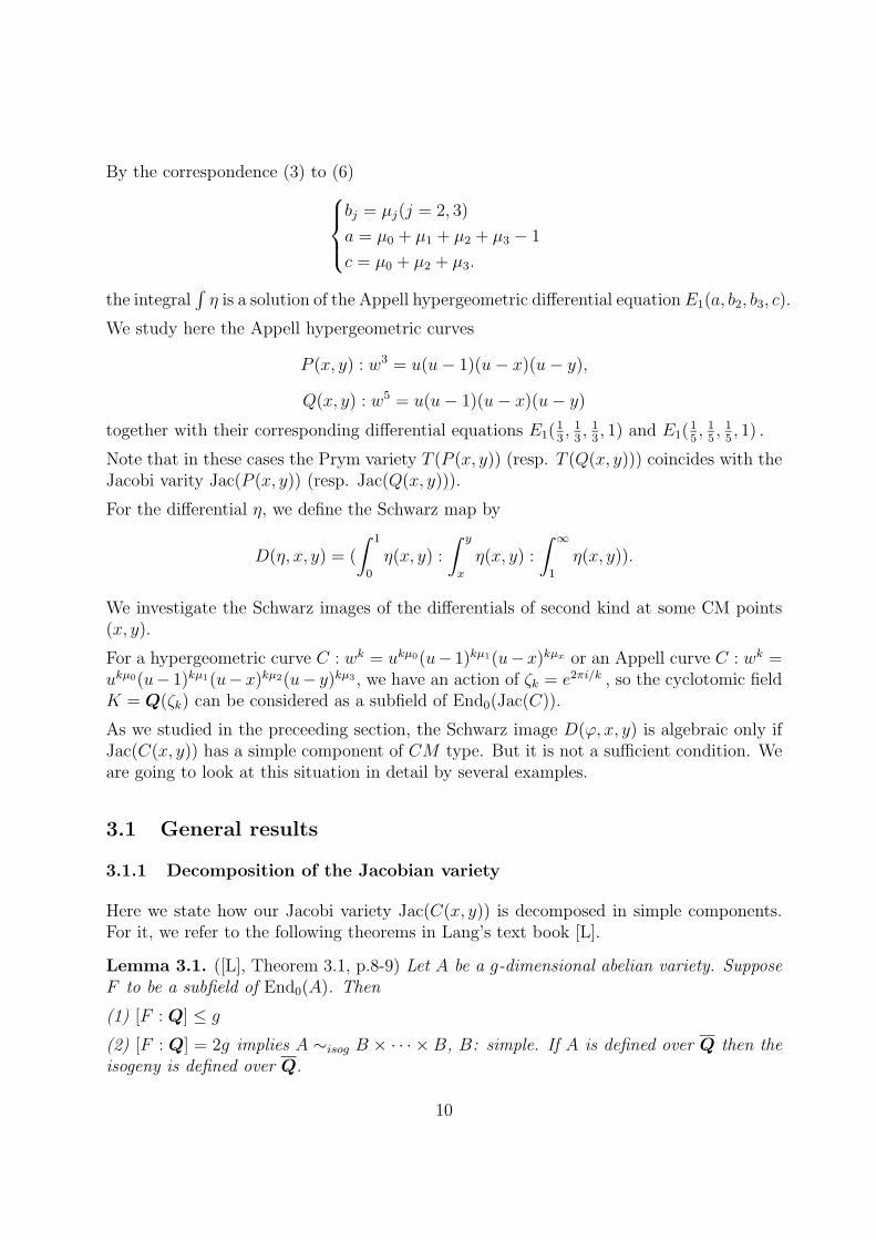
By the correspondence (3) to (6)

bj = µj(j = 2, 3)

a = µ0 + µ1 + µ2 + µ3 − 1

c = µ0 + µ2 + µ3.

the integral∫η is a solution of the Appell hypergeometric differential equationE1(a, b2, b3, c).

We study here the Appell hypergeometric curves

P (x, y) : w3 = u(u− 1)(u− x)(u− y),

Q(x, y) : w5 = u(u− 1)(u− x)(u− y)

together with their corresponding differential equations E1(13, 1

3, 1

3, 1) and E1(

15, 1

5, 1

5, 1) .

Note that in these cases the Prym variety T (P (x, y)) (resp. T (Q(x, y))) coincides with theJacobi varity Jac(P (x, y)) (resp. Jac(Q(x, y))).

For the differential η, we define the Schwarz map by

D(η, x, y) = (

∫ 1

0

η(x, y) :

∫ y

x

η(x, y) :

∫∞

1

η(x, y)).

We investigate the Schwarz images of the differentials of second kind at some CM points(x, y).

For a hypergeometric curve C : wk = ukµ0(u− 1)kµ1(u−x)kµx or an Appell curve C : wk =ukµ0(u− 1)kµ1(u−x)kµ2(u− y)kµ3 , we have an action of ζk = e2πi/k , so the cyclotomic fieldK = Q(ζk) can be considered as a subfield of End0(Jac(C)).

As we studied in the preceeding section, the Schwarz image D(ϕ, x, y) is algebraic only ifJac(C(x, y)) has a simple component of CM type. But it is not a sufficient condition. Weare going to look at this situation in detail by several examples.

3.1 General results

3.1.1 Decomposition of the Jacobian variety

Here we state how our Jacobi variety Jac(C(x, y)) is decomposed in simple components.For it, we refer to the following theorems in Lang’s text book [L].

Lemma 3.1. ([L], Theorem 3.1, p.8-9) Let A be a g-dimensional abelian variety. SupposeF to be a subfield of End0(A). Then

(1) [F : Q] ≤ g

(2) [F : Q] = 2g implies A ∼isog B × · · · × B, B: simple. If A is defined over Q then theisogeny is defined over Q.

10

Let X be a g -dimensional complex torus, and let F = Q(ξ) be a CM field of degree 2g.We assume that F ⊆ End0(X), and F to be a Galois extension of Q.

In this case we have a basis system ω1, · · · , ωg of holomorphic differentials which areeigendifferentials for the action of F . Set

ξ(ω1) = ξ1ω1, . . . , ξ(ωg) = ξgωg

We define the type Φ(F ) of the action of F by

Φ(F ) = (ξ1, . . . , ξg).

(ξ1, · · · , ξg) are conjugates of ξ. Together with their complex conjugates ξ1, · · · , ξg, ξ1, · · · , ξgbecomes a full set of conjugates of ξ. They correspond to 2g different embeddingsσ1, · · · , σg, σ1, · · · , σg of F into C with σj(ξ) = ξj. So Φ(F ) is a ”type” of F in the sense ofsubsection 1.2 with all dimVσ ≤ 1. In case X is an abelian variety, we say X is an abelianvariety of type (F,Φ).

Lemma 3.2. ([L], Theorem 3.5 (p.13))

Let A be an abelian variety of type (F,Φ). Set

H = σ ∈ Gal(F/Q) : σΦ = Φ

and suppose B to be a simple factor of A with K = End0(B). Then we have H =Gal(F/K). Especially H = 1 ⇐⇒ A is simple.

3.2 CM Picard curves

We consider the Picard curve

P (x, y) : w3 = u(u− 1)(u− x)(u− y) for xy(x− 1)(y − 1)(x− y) 6= 0

and differentials of second kind of the form

ϕ =uℓdu

wn.

We havegenus of P (x, y) = 3

We assume the variables x, y to be algebraic numbers. Set

ϕ1 = duw, ϕ2 = du

w2 , ϕ3 = uduw2 ,

ϕ4 = uduw, ϕ5 = u2du

w, ϕ6 = u2du

w2 .

(11)

11

They form a basis of the deRham cohomology group H1DR(P (x, y),Q) and the system

ϕ1, ϕ2, ϕ3 gives a basis of H0(P (x, y),Ω), the space of holomorphic differentials.

We note the following fact. If we know the algebraicity of D(ϕi, x, y) for a fixed point

(x, y) ∈ Q2

for every index i, it does not mean that we can see the algebraicity of D(ϕ, x, y)for a generic differential of H1

DR(P (x, y),Q).

Set ϕ = uℓduwn . Now we study the Schwarz values D(ϕ, 1+i

2, 1−i

2) for the special Picard curve

P (1+i2, 1−i

2) : w3 = u(u− 1)(u2 − u+ 1

2).

We have the following results

Theorem 3.1. For the Picard curve P (1+i2, 1−i

2) : y3 = x(x− 1)(x2 − x+ 1

2), we have

Jac(P (1 + i

2,1 − i

2)) ∼ E(ζ3) ⊕ E(i)2 ,

and

D(ϕ1;1 + i

2,1 − i

2), D(ϕ2;

1 + i

2,1 − i

2) ∈ Q,

D(ϕ3;1 + i

2,1 − i

2), D(ϕ4;

1 + i

2,1 − i

2), D(ϕ5;

1 + i

2,1 − i

2), D(ϕ6;

1 + i

2,1 − i

2) 6∈ Q.

Remark 3.1. Suppose n = 1 or 2 ( mod 3) and 0 ≤ ℓ ≤ 30. We have D(ϕ, 1+i2, 1−i

2) ∈

P 2(Q) if and only if ℓ = 0. This result illustrates our general Theorem 2.2 that insidesome Zariski open set Z we have at most 3 algebraic Schwarz values D(ϕ, τ) for varyingdifferentials ϕ ∈ Vn.

For the Schwarz values D(ϕ, ζ3, ζ23 ) corresponding to the special Picard curve P (ζ3, ζ

23 ) :

w3 = u(u3 − 1), we have:

Theorem 3.2. D(ϕ, ζ3, ζ23 ) ∈ P 2(Q) for any ℓ, n ∈ Z.

This fact illustrates that (ζ3, ζ23 ) belongs to the exceptional set C2 \ Z in Theorem 2.2.

Proof of Theorem 3.1

Set P = P (1+i2, 1−i

2) : w3 = u(u − 1)(u2 − u + 1

2), and set Σ : t3 = s4 − 1. We have a

biholomorphic isomorphism T : P → Σ over Q by

(s, t) = T (u,w) = (2u− 1, 243w).

The inverse is given by

(u,w) = T−1(s, t) = (1

2(s+ 1), 2−

43 t).

We use this isomorphism in our argument. Set

ψ1 = dst, ψ2 = ds

t2, ψ3 = sds

t2,

ψ4 = sdst, ψ5 = s2ds

t, ψ6 = s2ds

t2.

(12)

12

ψ1, ψ2, ψ3 forms a basis of H0(Σ,Ω), and ψ1, ψ2, · · · , ψ6 forms a basis of H1DR(Σ,Q).

We have the relation between 2 systems:

(T−1)∗ϕ1 = 16(1/3)2

ψ1

(T−1)∗ϕ2 = 16(2/3)2

ψ2

(T−1)∗ϕ3 = 16(2/3)4

ψ2 + 16(2/3)4

ψ3

(T−1)∗ϕ4 = 16(1/3)2

ψ1 + 16(1/3)2

ψ4

(T−1)∗ϕ5 = 16(1/3)4

ψ1 + 16(1/3)2

ψ4 + 16(1/3)4

ψ5

(T−1)∗ϕ6 = 16(2/3)4

ψ2 + 16(2/3)2

ψ3 + 16(2/3)4

ψ6.

(13)

We define paths α01, α12, α23 in the s space as indicated in Figure 1. Let α(k)j,j+1 be the path

on Σ with α(k+1)j,j+1 = ρα

(k)j,j+1 (j = 0, 1, 2), where ρ(s, t) = (s, ζ3t).

O 1

i

Α01Α12

Α23

Figure 1: paths for integrals on Σ

Let IP be the Q vector space generated by the periods

∫

γ

ϕi (i = 1, · · · , 6 , γ ∈ H1(P,Z)),

and let IΣ be the Q vector space generated by the integrals

∫

α(k)j,j+1

ψi (j = 0, 1, 2, k = 0, 1, i = 1, · · · , 6).

We can make up a basis of H1(Σ,Z) in terms of α(k)j,j+1. So we have IP = IΣ.

Here we note that

D(ϕ,1 + i

2,1 − i

2) ∈ P 2(Q) ⇐⇒

(∫

α(0)01

(T−1)∗(ϕ) :

∫

α(0)12

(T−1)∗(ϕ) :

∫

α(0)23

(T−1)∗(ϕ)

)∈ P 2(Q).

13

(a) Decomposition of Jac(Σ).

For the basis

ψ1 =ds

t, ψ2 =

ds

t2, ψ3 =

sds

t2,

F = Q(ζ12) acts by

σ : (s, w) 7→ (ζ3s, ζ4w) (ζ = ζ12). (14)

Set P0 : w′3 = s′2 − 1. The correspondence (s, w) 7→ (s′, w′) = (s2, w) defines a mapπ : P → P0 . The differential ψ3 is a lifting of the holomorphic differential on P0. So itinduces a projection H0(C,Ω) → H0(C0,Ω). Hence we have a decomposition

Jac(P ) ∼isog Jac(P0) ⊕B,

where B is the kernel of this projection. There is an action of F = Q(ζ12) on the space〈ψ1, ψ2〉 induced from (14).

Namelyσψ1 = ζ−1ψ1, σψ2 = ζ−5ψ2.

So we have the type Φ = (ζ−1, ζ−5) = (−1,−5) on B. By considering Lemma 3.2 andshifting Φ by the residue classes in (Z/12Z)∗ = 1, 5, 7, 11 we obtain

5(−1,−5) = (−1,−5) , 7(−1,−5) = (1, 5) , 11(−1,−5) = (1, 5) .

So we haveH = σ ∈ (Z/12Z)∗ : σΦ = Φ = 1, 5.

Hence B is non-simple, and by Lemma 3.1 it is a product of an elliptic curve with itself.By Lemma 3.2 again we know that B ∼isog E(i)2. Finally we obtain

Lemma 3.3.

Jac(P ) = Jac(Σ) ∼isog E(ζ3) ⊕ (E(i))2.

(b) By referring to Lemma 1.3 and the fact that E(i) and E(ζ3) are non–isogenous, theabove lemma induces

Lemma 3.4.

dimQ IP = dimQ IΣ = 4.

(c) Set pk =∫

α(0)01ψk. We can describe the period matrix of Σ with respect to the basis

ψ1, ψ2, ψ3 of H0(Σ,Ω) and the basis α(0)01 , α

(0)12 , α

(0)23 , α

(1)01 , α

(1)12 , α

(1)23 of H1(Σ,Q) in sym-

bolic notation by

Λ =

p1 ip1 −p1 ζ2

3p1 iζ23p1 −ζ2

3p1

p2 ip2 −p2 ζ3p2 iζ3p2 −ζ3p2

p3 −p3 p3 ζ3p3 −ζ3p3 ζ3p3

=

ψ1

ψ2

ψ3

(α

(0)01 , α

(0)12 , α

(0)23 , α

(1)01 , α

(1)12 , α

(1)23

).

14

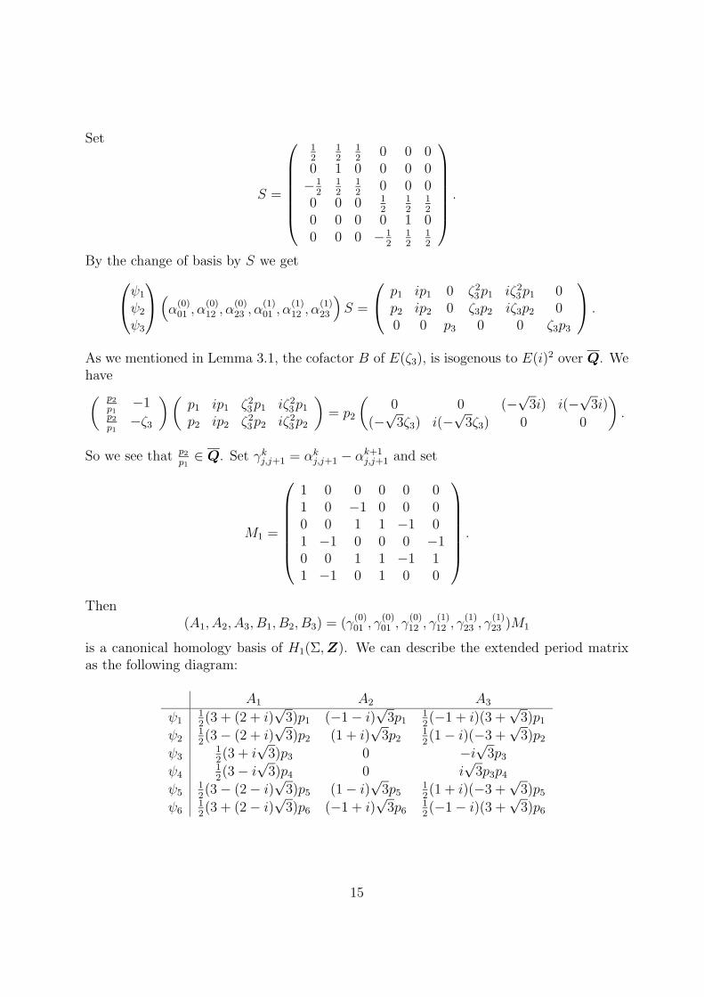
Set

S =

12

12

12

0 0 00 1 0 0 0 0−1

212

12

0 0 00 0 0 1

212

12

0 0 0 0 1 00 0 0 −1

212

12

.

By the change of basis by S we get

ψ1

ψ2

ψ3

(α

(0)01 , α

(0)12 , α

(0)23 , α

(1)01 , α

(1)12 , α

(1)23

)S =

p1 ip1 0 ζ2

3p1 iζ23p1 0

p2 ip2 0 ζ3p2 iζ3p2 00 0 p3 0 0 ζ3p3

.

As we mentioned in Lemma 3.1, the cofactor B of E(ζ3), is isogenous to E(i)2 over Q. Wehave( p2

p1−1

p2

p1−ζ3

)(p1 ip1 ζ2

3p1 iζ23p1

p2 ip2 ζ23p2 iζ2

3p2

)= p2

(0 0 (−

√3i) i(−

√3i)

(−√

3ζ3) i(−√

3ζ3) 0 0

).

So we see that p2

p1∈ Q. Set γk

j,j+1 = αkj,j+1 − αk+1

j,j+1 and set

M1 =

1 0 0 0 0 01 0 −1 0 0 00 0 1 1 −1 01 −1 0 0 0 −10 0 1 1 −1 11 −1 0 1 0 0

.

Then(A1, A2, A3, B1, B2, B3) = (γ

(0)01 , γ

(0)01 , γ

(0)12 , γ

(1)12 , γ

(1)23 , γ

(1)23 )M1

is a canonical homology basis of H1(Σ,Z). We can describe the extended period matrixas the following diagram:

A1 A2 A3

ψ112(3 + (2 + i)

√3)p1 (−1 − i)

√3p1

12(−1 + i)(3 +

√3)p1

ψ212(3 − (2 + i)

√3)p2 (1 + i)

√3p2

12(1 − i)(−3 +

√3)p2

ψ312(3 + i

√3)p3 0 −i

√3p3

ψ412(3 − i

√3)p4 0 i

√3p3p4

ψ512(3 − (2 − i)

√3)p5 (1 − i)

√3p5

12(1 + i)(−3 +

√3)p5

ψ612(3 + (2 − i)

√3)p6 (−1 + i)

√3p6

12(−1 − i)(3 +

√3)p6

15

B1 B2 B3

ψ112(−1 + i)(3 +

√3)p1

12(−1 + i)

√3(i+

√3)p1

12(−3 − (2 + i)

√3)p1

ψ212(1 − i)(−3 +

√3)p2

12(1 + i)(3i+

√3)p2

12(−3 + (2 + i)

√3)p2

ψ3 i√

3p3 0 12(3 + i

√3)p3

ψ4 −i√

3p3p4 0 12(3 − i

√3)p4

ψ512(1 + i)(−3 +

√3)p5

12(−1 − i)

√3(i+

√3)p5

12−3 + (2 − i)

√3p5

ψ612(−1 − i)(3 +

√3)p6

12(−1 + i)(3i+

√3)p6

12−3 − (2 − i)

√3p6

. According to Lemma 1.4 we obtain three nontrivial relations

p1p6 = − 3

3 +√

3π, p2p5 =

3

5(−3 +√

3)π, p3p4 = −

√3

2π. (15)

Combining it with p2/p1 ∈ Q we obtain p6/p5 ∈ Q. By Lemma 3.4 we obtain

Lemma 3.5. The Q vector space PΣ is generated by

p1, p2, · · · , p6,

and we have only two nontrivial linear relations p2/p1 ∈ Q and p6/p5 ∈ Q.

(d) By putting w3 = A(u) = u(u− 1)(u2 − u+ 12) we have dw3 = A′(u)du, hence

dw =1

3

A′(u)du

w2.

By observing d(uℓwm) = ℓuℓ−1wm +muℓwm−1dw we obtain

ℓuℓ−1wmdu ≡ −1

3muℓwm−3A′(u)du.

Therefore we have

Lemma 3.6. (1) If n ≡ 0 ( mod 3), then ϕ is an exact differential.

(2)xℓ+3dx

yn≡ 6ℓ− 6n+ 18

3ℓ− 4n+ 12

xℓ+2dx

yn− 9ℓ− 6n+ 18

6ℓ− 8n+ 24

xℓ+1dx

yn+

3ℓ− n+ 3

6ℓ− 8n+ 24

xℓdx

yn

(3)xℓdx

yn≡ 12ℓ− 16n+ 60

n− 3

xℓdx

yn−3− 6ℓ

n− 3

xℓ−1dx

yn−3

The equality (2) in the above lemma is essentially a contiguity relation between Appell’shypergeometric functions.

(e) Because ψk is an eigendifferential for the action of Q(ζ12), we have always(∫

α(0)01

ψk :

∫

α(0)12

ψk :

∫

α(0)23

ψk

)∈ P 2(Q) for all k = 1, 2, . . . , 6 .

16

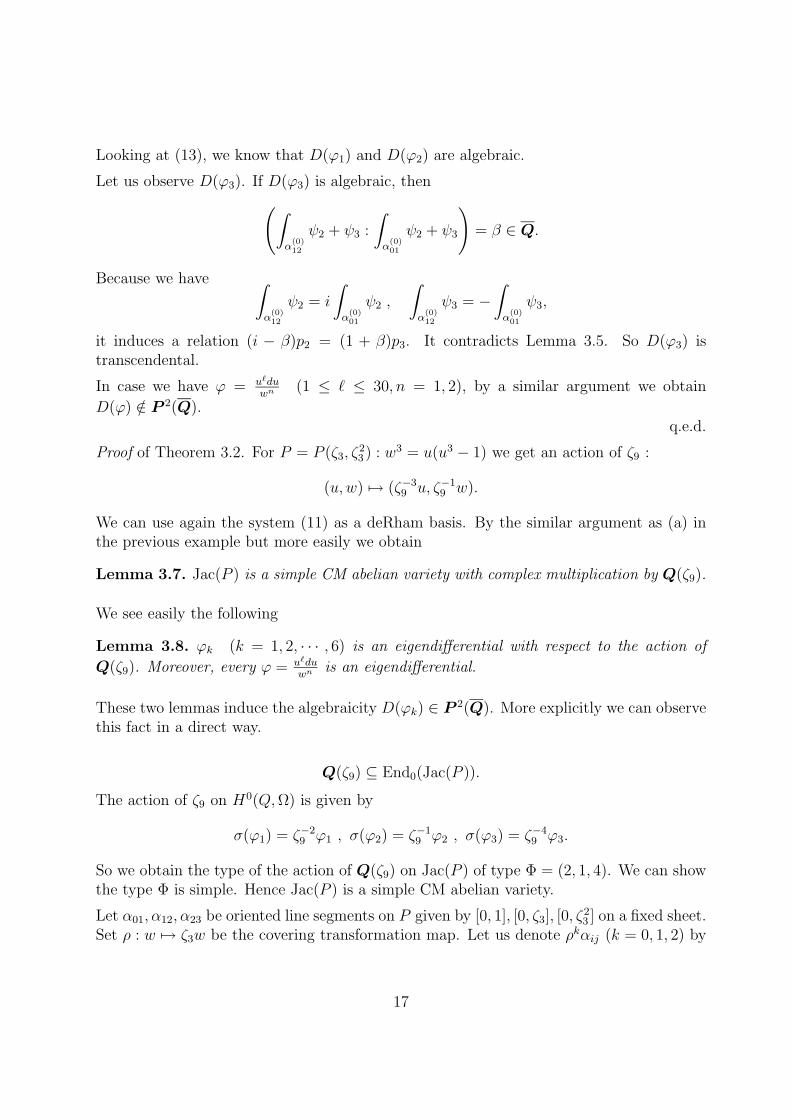
Looking at (13), we know that D(ϕ1) and D(ϕ2) are algebraic.

Let us observe D(ϕ3). If D(ϕ3) is algebraic, then

(∫

α(0)12

ψ2 + ψ3 :

∫

α(0)01

ψ2 + ψ3

)= β ∈ Q.

Because we have ∫

α(0)12

ψ2 = i

∫

α(0)01

ψ2 ,

∫

α(0)12

ψ3 = −∫

α(0)01

ψ3,

it induces a relation (i − β)p2 = (1 + β)p3. It contradicts Lemma 3.5. So D(ϕ3) istranscendental.

In case we have ϕ = uℓduwn (1 ≤ ℓ ≤ 30, n = 1, 2), by a similar argument we obtain

D(ϕ) /∈ P 2(Q).q.e.d.

Proof of Theorem 3.2. For P = P (ζ3, ζ23 ) : w3 = u(u3 − 1) we get an action of ζ9 :

(u,w) 7→ (ζ−39 u, ζ−1

9 w).

We can use again the system (11) as a deRham basis. By the similar argument as (a) inthe previous example but more easily we obtain

Lemma 3.7. Jac(P ) is a simple CM abelian variety with complex multiplication by Q(ζ9).

We see easily the following

Lemma 3.8. ϕk (k = 1, 2, · · · , 6) is an eigendifferential with respect to the action of

Q(ζ9). Moreover, every ϕ = uℓduwn is an eigendifferential.

These two lemmas induce the algebraicity D(ϕk) ∈ P 2(Q). More explicitly we can observethis fact in a direct way.

Q(ζ9) ⊆ End0(Jac(P )).

The action of ζ9 on H0(Q,Ω) is given by

σ(ϕ1) = ζ−29 ϕ1 , σ(ϕ2) = ζ−1

9 ϕ2 , σ(ϕ3) = ζ−49 ϕ3.

So we obtain the type of the action of Q(ζ9) on Jac(P ) of type Φ = (2, 1, 4). We can showthe type Φ is simple. Hence Jac(P ) is a simple CM abelian variety.

Let α01, α12, α23 be oriented line segments on P given by [0, 1], [0, ζ3], [0, ζ23 ] on a fixed sheet.

Set ρ : w 7→ ζ3w be the covering transformation map. Let us denote ρkαij (k = 0, 1, 2) by

17

α(k)ij . Put γ

(k)i = α

(k)ij − α

(k+1)ij (k = 0, 1). Putting

M2 =

−1 0 0 0 0 0−1 0 −1 0 0 01 1 1 0 0 10 1 1 −1 1 10 −1 −1 1 0 −11 −1 0 1 −1 0

,

(A1, A2, A3, B1, B2, B3) = (γ(0)01 , γ

(0)01 , γ

(0)12 , γ

(1)12 , γ

(1)23 , γ

(1)23 )M2

becomes a symplectic basis of H1(P,Z). By putting q =∫

α(0)01ϕ we obtain the following

table of integrals.

α(0)01 α

(0)12 α

(0)23 α

(1)01 α

(1)12 α

(1)23 α

(2)01 α

(2)12 α

(2)23

xmdxyn q ζ−n

3 q ζ−2n3 q ζm+1

3 q ζm−n+13 q ζm−2n+1

3 q ζ2m+23 q ζ2m−n+2

3 q ζ2m−2n+23 q .

So we can see D(ϕ) ∈ Q.

3.3 CM Pentagonal curves

Let us consider the following pentagonal curve

Q(λ, µ) : y5 = x(x− 1)(x− λ)(x− µ) for (λµ(λ− 1)(µ− 1)(λ− µ) 6= 0).

This is a curve of genus 6, and we have the following deRham basis:

1st kind : ϕ1 =dx

y2, ϕ2 =

dx

y3, ϕ3 =

xdx

y3, ϕ4 =

dx

y4, ϕ5 =

xdx

y4, ϕ6 =

x2dx

y4,

2nd kind : ϕ7 =dx

y, ϕ8 =

xdx

y, ϕ9 =

x2dx

y, ϕ10 =

xdx

y2, ϕ11 =

x2dx

y2, ϕ12 =

x2dx

y3.

For the special CM point (x, y) = (1+i2, 1−i

2), we have the following

Theorem 3.3.

D(ϕ1;1 + i

2,1 − i

2), D(ϕ2;

1 + i

2,1 − i

2), D(ϕ4;

1 + i

2,1 − i

2), D(ϕ7;

1 + i

2,1 − i

2) ∈ Q,

D(ϕ3;1 + i

2,1 − i

2), D(ϕ5;

1 + i

2,1 − i

2), D(ϕ6;

1 + i

2,1 − i

2), D(ϕ8;

1 + i

2

1 − i

2),

D(ϕ9;1 + i

2,1 − i

2), D(ϕ10;

1 + i

2,1 − i

2), D(ϕ11;

1 + i

2,1 − i

2), D(ϕ12;

1 + i

2,1 − i

2) /∈ Q.

18

Remark 3.2. We expect that we have D(xℓdxym ; 1+i

2, 1−i

2) /∈ Q for all 1 ≤ ℓ and all 1 ≤

m ≤ 4.

Proof of the theorem.

SetΣ1 : w5 = s4 − 1.

Then we have a deRham basis on Σ1:

1st kind : ψ1 =ds

w2, ψ2 =

ds

w3, ψ3 =

sds

w3, ψ4 =

ds

w4, ψ5 =

sds

w4, ψ6 =

s2ds

w4,

2nd kind : ψ7 =ds

w, ψ8 =

sds

w, ψ9 =

s2ds

w, ψ10 =

sds

w2, ψ11 =

s2ds

w2, ψ12 =

s2ds

w3.

We have two cyclic actions by ζ4 and ζ5 on Σ1:

(s, w) 7→ (ζ4s, w) , (s, w) 7→ (s, ζ5w).

They are generated by a single action

(s, w) 7→ (ζ520s, ζ

420w).

And it induces an action of Q(ζ20) on the space of the deRham cohomology groupH1DR(Σ1,Q).

NamelyQ(ζ20) ⊆ End0(Jac(Σ1)).

Every ψi (1 ≤ i ≤ 12) is an eigen differential for this action. Define

T : s(x) = 2x− 1, w(y) = 245y.

The CM curve Σ1 is shifted to the pentagonal curve

Q(1 + i

2,1 − i

2) : y5 = x(x− 1)(x2 − x+

1

2).

SetC1 : w5 = u2 − 1.

By putting s 7→ u = s2, we have a double covering map Σ → C1. Hence, Jac(Σ1) isnonsimple and A1 = Jac(C1) is a component. Here the differentials

ψ3 =sds

w3, ψ5 =

sds

w4

are liftings of the differential on C1.

The action of ζ20 on the space of holomorphic differentials given by σ : (s, w) 7→ (ζ520s, ζ

420w)

is described as follows:

σ(ψ1) = ζ−320 ψ1, σ(ψ2) = ζ−7

20 ψ2, σ(ψ3) = ζ−110 ψ3, σ(ψ4) = ζ−11

20 ψ4, σ(ψ5) = ζ−310 ψ5, σ(ψ6) = ζ−1

20 ψ6.

19

Thus the cofactor of Jac(Σ1) has the CM type (1, 3, 7, 11). We can see easily this is asimple CM-type . So we have the decomposition

Jac(Σ1) ∼ A1 ⊕ A2 with dimA1 = 2 , dimA2 = 4,

Q(ζ10) = End0(JacA1),Q(ζ20) = End0(JacA2).

According to Lemma 1.3 we have

dimQ 〈∫

γi

ψk〉 = 12 (i = 1, ..., 12 , k = 1, ..., 12). (16)

Let α01, α12, α23 be the oriented arcs on Σ1 with the projection [1, i], [i,−1], [−1,−i] on the

same sheet, respectively. We make the exchange of the sheets by ρ : w 7→ ζ5w, and let α(k)ij

denote ρkαij (k = 0, 1, 2, 3, 4). Set γ(k)ij = α

(k)ij − α

(k+1)ij (k = 0, 1, 2, 3). By putting

M =

1 0 1 0 0 −1 0 0 0 0 0 00 0 0 0 0 −1 1 0 1 0 0 10 0 0 1 0 −1 0 0 1 0 0 00 0 0 0 0 −1 1 0 0 1 0 00 0 1 0 0 0 0 0 0 0 0 00 0 1 0 0 −1 0 0 1 0 0 10 0 0 0 0 −1 0 0 2 0 0 10 0 0 0 0 −1 0 0 1 0 0 00 1 0 0 0 1 0 0 0 0 0 00 0 1 0 0 0 0 1 0 0 0 00 0 0 0 1 0 0 0 1 0 0 10 0 0 0 0 0 0 1 1 0 1 0

we have a symplectic basis

(A1, A2, A3, A4, A5, A6, B1, B2, B3, B4, B5, B6)

= (γ(0)01 , γ

(1)01 , γ

(2)01 , γ

(3)01 , γ

(0)12 , γ

(1)12 , γ

(2)12 , γ

(3)12 , γ

(0)23 , γ

(1)23 , γ

(2)23 , γ

(3)23 )M

of H1(Σ1,Z). The extended period matrix of Σ1 with respect to the basis

α(0)01 , α

(1)01 , α

(2)01 , α

(3)01 , α

(0)12 , α

(1)12 , α

(2)12 , α

(3)12 , α

(0)23 , α

(1)23 , α

(2)23 , α

(3)23 is given by the following table.

α(0)01 α

(1)01 α

(2)01 α

(3)01 α

(0)12 α

(1)12 α

(2)12 α

(3)12 α

(0)23 α

(1)23 α

(2)23 α

(3)23

ψ1 p1 ζ35p1 ζ1

5p1 ζ45p1 ip1 iζ3

5p1 iζ15p1 iζ4

5p1 −p1 −ζ35p1 −ζ1

5p1 −ζ45p1

ψ2 p2 ζ25p2 ζ4

5p2 ζ15p2 ip2 iζ2

5p2 iζ45p2 iζ1

5p2 −p2 −ζ25p2 −ζ4

5p2 −ζ15p2

ψ3 p3 ζ25p3 ζ4

5p3 ζ15p3 −p3 −ζ2

5p3 −ζ45p3 −ζ1

5p3 p3 ζ25p3 ζ4

5p3 ζ15p3

ψ4 p4 ζ15p4 ζ2

5p4 ζ35p4 ip4 iζ1

5p4 iζ25p4 iζ3

5p4 −p4 −ζ15p4 −ζ2

5p4 −ζ35p4

ψ5 p5 ζ15p5 ζ2

5p5 ζ35p5 −p5 −ζ1

5p5 −ζ25p5 −ζ3

5p5 p5 ζ15p5 ζ2

5p5 ζ35p5

ψ6 p6 ζ15p6 ζ2

5p6 ζ35p6 −ip6 −iζ1

5p6 −iζ25p6 −iζ3

5p6 −p6 −ζ15p6 −ζ2

5p6 −ζ35p6

ψ7 q1 ζ45q1 ζ3

5q1 ζ25q1 iq1 iζ4

5q1 iζ35q1 iζ2

5q1 −q1 −ζ45q1 −ζ3

5q1 −ζ25q1

ψ8 q2 ζ45q2 ζ3

5q2 ζ25q2 −q2 −ζ4

5q2 −ζ35q2 −ζ2

5q2 q2 ζ45q2 ζ3

5q2 ζ25q2

ψ9 q3 ζ45q3 ζ3

5q3 ζ25q3 −iq3 −iζ4

5q3 −iζ35q3 −iζ2

5q3 −q3 −ζ45q3 −ζ3

5q3 −ζ25q3

ψ10 q4 ζ35q4 ζ1

5q4 ζ45q4 −q4 −ζ3

5q4 −ζ15q4 −ζ4

5q4 q4 ζ35q4 ζ1

5q4 ζ45q4

ψ11 q5 ζ35q5 ζ1

5q5 ζ45q5 −iq5 −iζ3

5q5 −iζ15q5 −iζ4

5q5 −q5 −ζ35q5 −ζ1

5q5 −ζ45q5

ψ12 q6 ζ25q6 ζ4

5q6 ζ15q6 −iq6 −iζ2

5q6 −iζ45q6 −iζ1

5q6 −q6 −ζ25q6 −ζ4

5q6 −ζ15q6

20

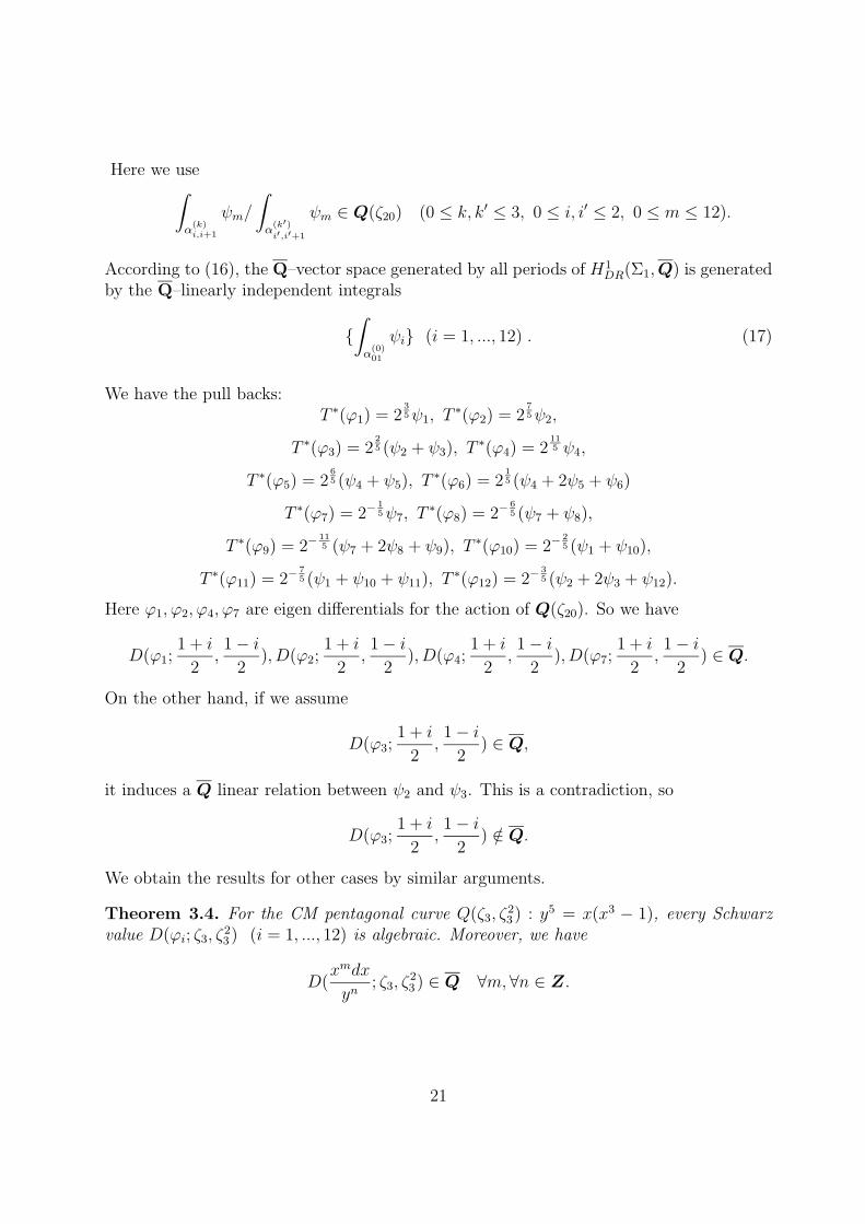
Here we use∫

α(k)i,i+1

ψm/

∫

α(k′)

i′,i′+1

ψm ∈ Q(ζ20) (0 ≤ k, k′ ≤ 3, 0 ≤ i, i′ ≤ 2, 0 ≤ m ≤ 12).

According to (16), the Q–vector space generated by all periods of H1DR(Σ1,Q) is generated

by the Q–linearly independent integrals

∫

α(0)01

ψi (i = 1, ..., 12) . (17)

We have the pull backs:T ∗(ϕ1) = 2

35ψ1, T

∗(ϕ2) = 275ψ2,

T ∗(ϕ3) = 225 (ψ2 + ψ3), T

∗(ϕ4) = 2115 ψ4,

T ∗(ϕ5) = 265 (ψ4 + ψ5), T

∗(ϕ6) = 215 (ψ4 + 2ψ5 + ψ6)

T ∗(ϕ7) = 2−15ψ7, T

∗(ϕ8) = 2−65 (ψ7 + ψ8),

T ∗(ϕ9) = 2−115 (ψ7 + 2ψ8 + ψ9), T

∗(ϕ10) = 2−25 (ψ1 + ψ10),

T ∗(ϕ11) = 2−75 (ψ1 + ψ10 + ψ11), T

∗(ϕ12) = 2−35 (ψ2 + 2ψ3 + ψ12).

Here ϕ1, ϕ2, ϕ4, ϕ7 are eigen differentials for the action of Q(ζ20). So we have

D(ϕ1;1 + i

2,1 − i

2), D(ϕ2;

1 + i

2,1 − i

2), D(ϕ4;

1 + i

2,1 − i

2), D(ϕ7;

1 + i

2,1 − i

2) ∈ Q.

On the other hand, if we assume

D(ϕ3;1 + i

2,1 − i

2) ∈ Q,

it induces a Q linear relation between ψ2 and ψ3. This is a contradiction, so

D(ϕ3;1 + i

2,1 − i

2) /∈ Q.

We obtain the results for other cases by similar arguments.

Theorem 3.4. For the CM pentagonal curve Q(ζ3, ζ23 ) : y5 = x(x3 − 1), every Schwarz

value D(ϕi; ζ3, ζ23 ) (i = 1, ..., 12) is algebraic. Moreover, we have

D(xmdx

yn; ζ3, ζ

23 ) ∈ Q ∀m,∀n ∈ Z.

21

proof. Let α01, α12, α23 be the oriented arcs on Σ1 with the projection [0, 1], [0, ζ3], [0, ζ23 ]

on the same sheet, respectively. We make the exchange of the sheets by ρ : w 7→ ζ5w, andlet α

(k)ij denote ρkαij (k = 0, 1, 2, 3, 4). Set γ

(k)ij = α

(k)ij − α

(k+1)ij (k = 0, 1, 2, 3). By putting

M =

0 1 0 0 0 1 0 0 0 0 0 00 0 1 0 0 0 0 1 0 0 0 00 0 0 0 1 0 0 0 1 0 0 10 0 0 0 0 0 0 1 1 0 1 01 0 0 0 0 −1 0 0 0 0 0 00 0 −1 0 0 0 1 0 0 0 0 00 0 0 1 0 0 0 0 −1 0 0 −10 0 0 0 0 0 1 0 −1 1 0 00 −1 1 0 0 −1 0 0 0 0 0 00 0 0 0 0 −1 0 −1 1 0 0 10 0 0 0 −1 −1 0 0 1 0 0 00 0 0 0 0 −1 0 −1 0 0 −1 0

,

we obtain a symplectic basis

(A1, A2, A3, A4, A5, A6, B1, B2, B3, B4, B5, B6)

= (γ(0)01 , γ

(1)01 , γ

(2)01 , γ

(3)01 , γ

(0)12 , γ

(1)12 , γ

(2)12 , γ

(3)12 , γ

(0)23 , γ

(1)23 , γ

(2)23 , γ

(3)23 )M

of H1(Q(ζ3, ζ23 ),Z). We have the following table of path integrals

α(0)01 α

(0)12 α

(0)23 α

(1)01 α

(1)12 α

(1)23

xmdxyn q ωm+1q ω2m+2q ζ−n

5 q ωm+1ζ−n5 q ω2m+2ζ−n

5 q

α(2)01 α

(2)12 α

(2)23 α

(3)01 α

(3)12 α

(3)23

ζ−2n5 q ωm+1ζ−2n

5 q ω2m+2ζ−2n5 q ζ−3n

5 q ωm+1ζ−3n5 q ω2m+2ζ−3n

5 q,

namely we have

∫

α(k)i,i+1

xmdx

yn/

∫

α(k′)

i′,i′+1

xmdx

yn∈ Q(ζ15) (0 ≤ k, k′ ≤ 3, 0 ≤ i, i′ ≤ 2).

So we obtain the required result.

We can make the argument by the decomposition of the Jacobian varity instead of theabove direct proof. We have an action of ζ15 on Q(ζ3, ζ

23 ):

σ : (x, y) 7→ (ζ515x, ζ

115y).

HenceQ(ζ15) ⊆ End0(Jac(C(ζ3, ζ

23 ))).

22

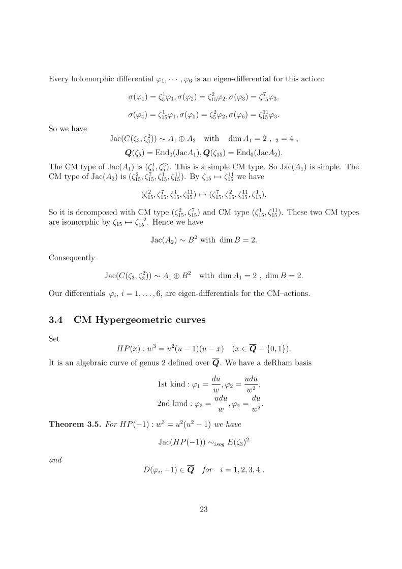
Every holomorphic differential ϕ1, · · · , ϕ6 is an eigen-differential for this action:

σ(ϕ1) = ζ15ϕ1, σ(ϕ2) = ζ2

15ϕ2, σ(ϕ3) = ζ715ϕ3,

σ(ϕ4) = ζ115ϕ1, σ(ϕ5) = ζ2

5ϕ2, σ(ϕ6) = ζ1115ϕ3.

So we haveJac(C(ζ3, ζ

23 )) ∼ A1 ⊕ A2 with dimA1 = 2 , 2 = 4 ,

Q(ζ5) = End0(JacA1),Q(ζ15) = End0(JacA2).

The CM type of Jac(A1) is (ζ15 , ζ

25 ). This is a simple CM type. So Jac(A1) is simple. The

CM type of Jac(A2) is (ζ215, ζ

715, ζ

115, ζ

1115 ). By ζ15 7→ ζ11

15 we have

(ζ215, ζ

715, ζ

115, ζ

1115 ) 7→ (ζ7

15, ζ215, ζ

1115 , ζ

115).

So it is decomposed with CM type (ζ215, ζ

715) and CM type (ζ1

15, ζ1115 ). These two CM types

are isomorphic by ζ15 7→ ζ−215 . Hence we have

Jac(A2) ∼ B2 with dimB = 2.

Consequently

Jac(C(ζ3, ζ23 )) ∼ A1 ⊕B2 with dimA1 = 2 , dimB = 2.

Our differentials ϕi, i = 1, . . . , 6, are eigen-differentials for the CM–actions.

3.4 CM Hypergeometric curves

SetHP (x) : w3 = u2(u− 1)(u− x) (x ∈ Q − 0, 1).

It is an algebraic curve of genus 2 defined over Q. We have a deRham basis

1st kind : ϕ1 =du

w, ϕ2 =

udu

w2,

2nd kind : ϕ3 =udu

w, ϕ4 =

du

w2.

Theorem 3.5. For HP (−1) : w3 = u2(u2 − 1) we have

Jac(HP (−1)) ∼isog E(ζ3)2

andD(ϕi,−1) ∈ Q for i = 1, 2, 3, 4 .

23

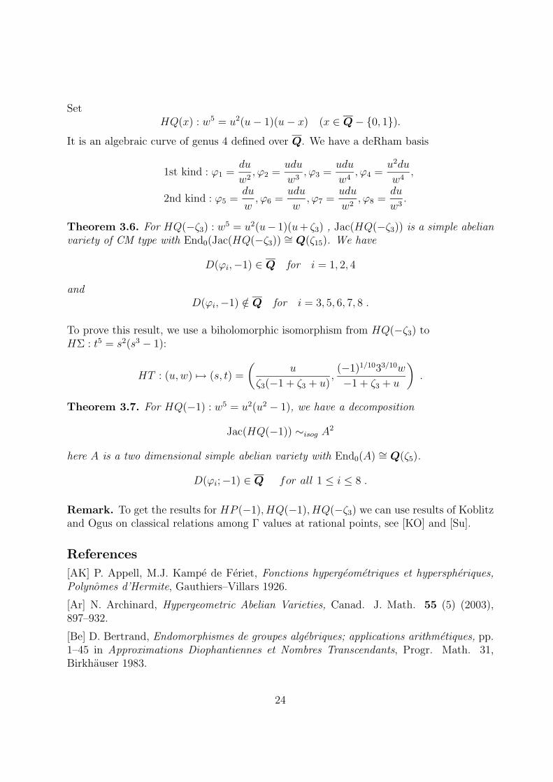
SetHQ(x) : w5 = u2(u− 1)(u− x) (x ∈ Q − 0, 1).

It is an algebraic curve of genus 4 defined over Q. We have a deRham basis

1st kind : ϕ1 =du

w2, ϕ2 =

udu

w3, ϕ3 =

udu

w4, ϕ4 =

u2du

w4,

2nd kind : ϕ5 =du

w, ϕ6 =

udu

w, ϕ7 =

udu

w2, ϕ8 =

du

w3.

Theorem 3.6. For HQ(−ζ3) : w5 = u2(u− 1)(u+ ζ3) , Jac(HQ(−ζ3)) is a simple abelianvariety of CM type with End0(Jac(HQ(−ζ3)) ∼= Q(ζ15). We have

D(ϕi,−1) ∈ Q for i = 1, 2, 4

andD(ϕi,−1) /∈ Q for i = 3, 5, 6, 7, 8 .

To prove this result, we use a biholomorphic isomorphism from HQ(−ζ3) toHΣ : t5 = s2(s3 − 1):

HT : (u,w) 7→ (s, t) =

(u

ζ3(−1 + ζ3 + u),(−1)1/1033/10w

−1 + ζ3 + u

).

Theorem 3.7. For HQ(−1) : w5 = u2(u2 − 1), we have a decomposition

Jac(HQ(−1)) ∼isog A2

here A is a two dimensional simple abelian variety with End0(A) ∼= Q(ζ5).

D(ϕi;−1) ∈ Q for all 1 ≤ i ≤ 8 .

Remark. To get the results for HP (−1), HQ(−1), HQ(−ζ3) we can use results of Koblitzand Ogus on classical relations among Γ values at rational points, see [KO] and [Su].

References

[AK] P. Appell, M.J. Kampe de Feriet, Fonctions hypergeometriques et hyperspheriques,Polynomes d’Hermite, Gauthiers–Villars 1926.

[Ar] N. Archinard, Hypergeometric Abelian Varieties, Canad. J. Math. 55 (5) (2003),897–932.

[Be] D. Bertrand, Endomorphismes de groupes algebriques; applications arithmetiques, pp.1–45 in Approximations Diophantiennes et Nombres Transcendants, Progr. Math. 31,Birkhauser 1983.

24

[ChWe] Cl. Chevalley, A. Weil, Uber das Verhalten der Integrale 1. Gattung bei Automor-phismen des Funktionenkorpers, Abh. Hamburger Math. Sem. 10 (1934), 358–361.

[CW1] P.B. Cohen, J. Wolfart, Algebraic Appell–Lauricella Functions, Analysis 12 (1992),359–376.

[CW2] P.B. Cohen, J. Wolfart, Fonctions hypergeometriques en plusieurs variables et es-paces des modules de varietes abeliennes, Ann. scient. Ec. Norm. Sup. 26 (1993),665–690.

[GH] Ph. Griffiths, J. Harris, Principles of Algebraic Geometry, Wiley 1978

[Kl] F. Klein, Vorlesungen uber die hypergeometrische Funktion, Springer 1933.

[KO] N. Koblitz, A. Ogus, Algebraicity of some products of values of the Γ function, Proc.Symp. Pure Math. 33 (1979), 343–346

[Ko] K. Koike, On the family of pentagonal curves of genus 6 and associated modular formson the ball, J. Math. Soc. Japan, 55 (2003), 165–196.

[L] S. Lang, Complex Multiplication, Springer 1983.

[Sa] T. Sasaki, On the finiteness of the monodromy group of the system of hypergeometricdifferential equations (FD) , J. Fac. Sci. Univ. of Tokyo 24 (1977), 565–573.

[Schw] H.A. Schwarz, Uber diejenigen Falle, in welchen die Gaußische hypergeometrischeReihe eine algebraische Funktion ihres vierten Elements darstellt, J. Reine Angew. Math.75 (1873), 292–335.

[STW] H. Shiga, T. Tsutsui, J. Wolfart, Fuchsian differential equations with apparentsingularities, with an appendix by P.B. Cohen, Osaka J. Math. 41 (2004), 625–658.

[SW1] H. Shiga, J. Wolfart, Criteria for complex multiplication and transcendence proper-ties for automorphic functions, J. reine angew. Math. 463 (1995), 1–25.

[SW2] H. Shiga, J. Wolfart, Algebraic Values of Schwarz Triangle Functions, pp. 287–312in Arithmetic and Geometry Around Hypergeometric Functions, ed. by R.-P. Holzapfel,A.M. Uludag, M. Yoshida, Birkhauser PM 260, 2007.

[Sh] G. Shimura, On analytic families of polarized abelian varieties and automorphic func-tions, Ann. Math. 78 (1963), 149–192.

[ShT] G. Shimura, Y. Taniyama, Complex multiplication of abelian varieties and its appli-cations to number theory, Publ. Math. Soc. Japan 6, 1961.

[Si] C.L. Siegel, Lectures on Riemann Matrices, Tata Inst., Bombay 1963.

[Su] Y. Suzuki, Periods of hypergeometric curves, Technical Report, Chiba University 2008.

[Wu] G. Wustholz, Algebraische Punkte auf analytischen Untergruppen algebraischer Grup-pen, Ann. of Math. 129 (1989), 501–517.

[Y] M. Yoshida, Fuchsian Differential Equations, Aspects of Mathematics E11, Vieweg1987.

25

Address of the Authors

Hironori Shiga, Yoshio Suzuki

Inst. of Math. and PhysicsChiba UniversityYayoi–Cho 1–33, Inage–kuChiba 263–8522Japane–mail: shiga@math.s.chiba-u.ac.jp

Jurgen Wolfart

Math. Seminar der Univ.Postfach 111 932D–60054 Frankfurt a.M.Germanye–mail: wolfart@math.uni-frankfurt.de

26