Arithmetic Geometry and Analysis on Foliated

Spaces

Christopher Deninger

May 23, 2005

1 Introduction

For the arithmetic study of varieties over finite fields powerful cohomolog-ical methods are available which in particular shed much light on the na-ture of the corresponding zeta functions. These investigations culminated inDeligne’s proof of an analogue of the Riemann conjecture for such zeta func-tions. This had been the hardest part of the Weil conjectures. For algebraicschemes over spec Z and in particular for the Riemann zeta function no co-homology theory has yet been developed that could serve similar purposes.For a long time it had even been a mystery how such a theory could look likeeven formally. In these lectures we first describe the shape that a cohomolog-ical formalism for algebraic schemes over the integers should take. We thendiscuss how it would relate to conjectures on arithmetic zeta-functions andindicate a couple of consequences of the formalism that can be proved usingstandard methods. As it turns out there is a large class of dynamical sys-tems on foliated manifolds whose reduced leafwise cohomology has severalof the expected structural properties of the desired cohomology for algebraicschemes. Comparing the arithmetic and dynamical pictures leads to someinsight into the basic geometric structures that dynamical systems relevantfor L-functions of varieties over number fields should have. We also discussrelations between these ideas on dynamical systems and “Arithmetic Topol-ogy”. In that subject one studies analogies between number theory and thetheory of 3-manifolds.

The present report was written for a lecture series at the SouthwesternCenter for Arithmetic Algebraic Geometry at the University of Arizona. Itis mostly based on the papers [16], [17] and [18], properly updated.

I would like to thank Minhyong Kim very much for the invitation to givethese lectures.

1

2 Geometric zeta- and L-functions

Consider the Dedekind zeta function of a number field K/Q

ζK(s) =∏p

(1−Np−s)−1 =∑

a

Na−s for Re s > 1 .

Here, p runs over the prime ideals of the ring of integers o = oK of K. Thefunction ζK(s) has a holomorphic continuation to C\1 with a simple poleat s = 1. To its finite Euler factors

ζp(s) = (1−Np−s)−1

we add Euler factors corresponding to the archimedian places p |∞ of K

ζp(s) =

2−1/2 π−s/2 Γ(s/2) if p |∞ is real(2π)−sΓ(s) if p |∞ is complex

The completed zeta function

ζK(s) = ζK(s)∏p |∞

ζp(s)

is holomorphic in C \ 0, 1 with simple poles at s = 0, 1 and satisfies thefunctional equation:

ζK(1− s) = |dK |s−1/2ζK(s) .

Here dK is the discriminant of K over Q. The zeroes of ζK(s) are the socalled non-trivial zeroes of ζK(s), i.e. those in the critical strip 0 < Re s < 1.The famous Riemann conjecture for K asserts that they all lie on the lineRe s = 1/2.Apart from its zeroes, the special values of ζK(s), i.e. the numbers ζK(n) forintegers n ≥ 2, have received a great deal of attention. There are two sets ofconjectures expressing these values in cohomological terms. One by Blochand Kato [8] which has been verified for all abelian extension K/Q, andanother more recent one by Lichtenbaum [32]. Together with the theory ofζ-functions of curves over finite fields this suggests that the Dedekind zetafunction should be cohomological in nature. The rest of this article will bedevoted to a thorough discussion of this hypothesis in a broader context.

A natural generalization of the Riemann zeta function to the context ofarithmetic geometry is the Hasse–Weil zeta function ζX (s) of an algebraicscheme X/Z

ζX (s) =∏

x∈|X |

(1−N(x)−s)−1 , Re s > dimX

2

where |X | is the set of closed points of X and N(x) is the number of elementsin the residue field of x. For X = specOK we recover the Dedekind zetafunction of K. It is expected that ζX (s) has a meromorphic continuation toC and, if X is regular and proper over spec Z, that

ζX (s) = ζX (s)ζX∞(s)

has a simple functional equation with respect to the substitution of s bydimX − s. Here ζX∞(s) is a certain product of Γ-factors depending on theHodge structure on the cohomology of X∞ = X ⊗ R. This functional equa-tion is known if X is equicharacteristic, i.e. an Fp-scheme for some p, byusing the Lefschetz trace formula and Poincare duality for l-adic cohomol-ogy.The present strategy for approaching ζX (s) was first systematically formu-lated by Langlands. He conjectured that every Hasse–Weil zeta function isup to finitely many Euler factors the product of automorphic L-functions.One could then apply the theory of these L-functions which is quite welldeveloped in important cases although by no means in general. For X withgeneric fibre related to Shimura varieties this Langlands program has beenachieved in very interesting examples. Another spectacular instance wasWiles’ proof with Taylor of modularity for most elliptic curves over Q.The strategy outlined in section 3 of the present article is completely differ-ent and much closer to the cohomological methods in characteristic p.By the work of Deligne [11], it is known that for proper regular X/Fp thezeroes (resp. poles) of ζX (s) = ζX (s) have real parts equal to ν/2 for odd(resp. even) integers 0 ≤ ν ≤ 2 dimX , and one may wonder whether thesame is true for the completed Hasse Weil zeta function ζX (s) of an arbitraryproper and regular scheme X/Z.As for the orders of vanishing at the integers, a conjecture of Soule [43] as-serts that for X/Z regular, quasi-projective connected and of dimension d,we have the formula

(1) ords=d−nζX (s) =2n∑i=0

(−1)i+1 dimH iM(X ,Q(n)) .

Here, H iM(X ,Q(n)) is the rational motivic cohomology of X which can be

defined by the formula

H iM(X ,Q(n)) = Gr n

γ (K2n−i(X )⊗Q) .

The associated graded spaces are taken with respect to the γ-filtration onalgebraic K-theory. Unfortunately it is not even known, except in specialcases, whether the dimensions on the right hand side are finite.

3

3 The conjectural cohomological formalism

In this section we interpret some of the conjectures about zeta-functions interms of an as yet speculative infinite dimensional cohomology theory. Wealso describe a number of consequences of this very rigid formalism thatcan be proved directly. Among these there is a formula which expressesthe Dedekind ζ-function as a zeta-regularized product. After giving thedefinition of regularized determinants in a simple algebraic setting we firstdiscuss the formalism in the case of the Dedekind zeta function and thengeneralize to Hasse–Weil zeta functions.

Given a C-vector space H with an endomorphism Θ such that H is thecountable sum of finite dimensional Θ-invariant subspaces Hα, the spectrumsp (Θ) is defined as the union of the spectra of Θ on Hα, the eigenvaluesbeing counted with their algebraic multiplicities. The (zeta-)regularizeddeterminant det∞(Θ |H) of Θ is defined to be zero if 0 ∈ sp (Θ), and by theformula

(2) det∞(Θ |H) :=∏

α∈sp (Θ)

α := exp(−ζ ′Θ(0))

if 0 /∈ sp (Θ). Here

ζΘ(s) =∑

0 6=α∈sp (Θ)

α−s , where − π < argα ≤ π ,

is the spectral zeta function of Θ. For (2) to make sense we require that ζΘbe convergent in some right half plane, with meromorphic continuation toRe s > −ε, for some ε > 0, holomorphic at s = 0. For an endomorphism Θ0

on a real vector space H0, such that Θ = Θ0 ⊗ id on H = H0 ⊗ C satisfiesthe above requirements, we set

det∞(Θ0 |H0) = det∞(Θ |H) .

On a finite dimensional vector space H we obtain the ordinary determinantof Θ. As an example of a regularized determinant, consider an endomor-phism Θ whose spectrum consists of the number 1, 2, 3, . . . with multiplicitiesone. Then

det∞(Θ |H) =∞∏

ν=1

ν =√

2π since ζ ′(0) = − log√

2π .

The regularized determinant plays a role for example in Arakelov theoryand in string theory. In our context it allows us to write the different Euler

4

factors of zeta-functions in a uniform way as we will first explain for theDedekind zeta function.

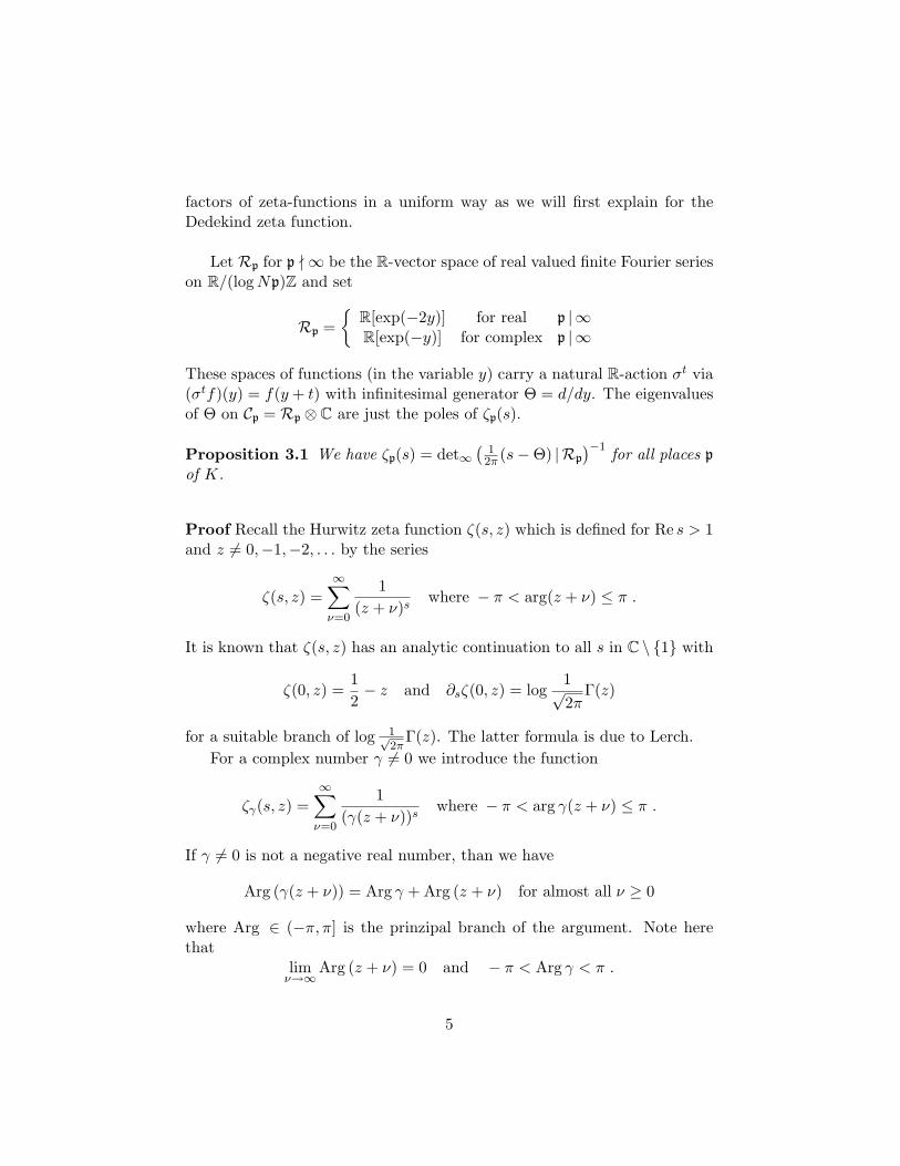
Let Rp for p -∞ be the R-vector space of real valued finite Fourier serieson R/(logNp)Z and set

Rp =

R[exp(−2y)] for real p |∞R[exp(−y)] for complex p |∞

These spaces of functions (in the variable y) carry a natural R-action σt via(σtf)(y) = f(y + t) with infinitesimal generator Θ = d/dy. The eigenvaluesof Θ on Cp = Rp ⊗ C are just the poles of ζp(s).

Proposition 3.1 We have ζp(s) = det∞(

12π (s−Θ) |Rp

)−1 for all places p

of K.

Proof Recall the Hurwitz zeta function ζ(s, z) which is defined for Re s > 1and z 6= 0,−1,−2, . . . by the series

ζ(s, z) =∞∑

ν=0

1(z + ν)s

where − π < arg(z + ν) ≤ π .

It is known that ζ(s, z) has an analytic continuation to all s in C \ 1 with

ζ(0, z) =12− z and ∂sζ(0, z) = log

1√2π

Γ(z)

for a suitable branch of log 1√2π

Γ(z). The latter formula is due to Lerch.For a complex number γ 6= 0 we introduce the function

ζγ(s, z) =∞∑

ν=0

1(γ(z + ν))s

where − π < arg γ(z + ν) ≤ π .

If γ 6= 0 is not a negative real number, than we have

Arg (γ(z + ν)) = Arg γ + Arg (z + ν) for almost all ν ≥ 0

where Arg ∈ (−π, π] is the prinzipal branch of the argument. Note herethat

limν→∞

Arg (z + ν) = 0 and − π < Arg γ < π .

5

Hence we haveζγ(s, z) = γ−sζ(s, z)

where ζ(s, z) differs from the Hurwitz zeta function in that finitely manyargument in its definition are possibly nonprincipal. Therefore, we still have

ζ(0, z) =12− z and exp(−∂sζ(0, z)) =

(1√2π

Γ(z))−1

and hence

ζγ(0, z) =12− z and exp(−∂sζγ(0, z)) = γ1/2−z

(1√2π

Γ(z))−1

i.e.∞∏

ν=0

γ(z + ν) = γ1/2−z

(1√2π

Γ(z))−1

.

In order to calculate∏

ν∈Z γ(z + ν) note that∑ν∈Z

1(γ(z + ν))s

= ζγ(s, z) + ζ−γ(s,−z)− (γz)−s .

Using the formula

1z

(1√2π

Γ(z))−1 (

1√2π

Γ(−z))−1

= i(eiπz − e−iπz)

which follows from the equation:

Γ(z)Γ(1− z) =π

sinπzwe get: ∏

ν∈Zγ(z + ν) =

1− e−2πiz if Im γ > 01− e2πiz if Im γ < 0

.

For p -∞ we have:

det∞

(12π

(s− θ) |Rp

)=

∏ν∈Z

12π

(s− 2πiν

logNp

)=

∏ν∈Z

i

logNp

(s logNp

2πi− ν

)= 1− exp

(−2πi

s logNp

2πi

)= 1−Np−s = ζp(s)−1

6

for real p |∞ on the other hand we find

det∞

(12π

(s− θ) |Rp

)=

∞∏ν=0

12π

(s+ 2ν)

=∞∏

ν=0

1π

(s2

+ ν)

= πs2− 1

2

(1√2π

Γ(s

2

))−1

=√

2πs/2Γ(s

2

)−1= ζp(s)−1 .

Similarly, for complex p |∞ we get

det∞

(1

2πi(s− θ) |Rp

)=

∞∏ν=0

12π

(s+ ν)

= (2π)s− 12

(1√2π

Γ(s))−1

= (2π)sΓ(s)−1 = ζp(s)−1 .

2

In a sense spec o = spec o ∪ p |∞ is analogous to a projective curve Xover a finite field of characteristic p. For every constructible Ql-sheaf R onX with l 6= p one defines the zeta function of X and R by the Euler productover the closed points x of X

ζX (s,R) =∏x

det(1−N(x)−sFr∗x |Rx)−1 for Re s > 1 .

Here, Rx is the stalk of R in a geometric point x over x and Frx is theFrobenius morphism. Using the Grothendieck–Verdier–Lefschetz trace for-mula in characteristic p one gets the following cohomological expression forζX (s,R):

ζX (s,R) =2∏

i=0

det(1− p−sFr∗p |H iet(X ,R))(−1)i+1

.

Here, Frp is the absolute Frobenius morphism and X = X ⊗Fp Fp. Thisformula together with the proposition suggests by analogy that a formula ofthe following type might hold:

(3) ζK(s) =2∏

i=0

det∞(

12π (s−Θ) |H i

dyn(spec o,R))(−1)i+1

.

7

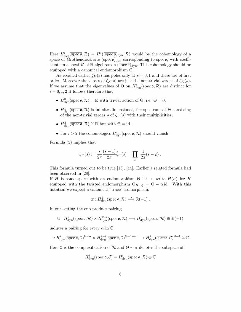
Here H idyn(spec o,R) = H i((spec o)dyn,R) would be the cohomology of a

space or Grothendieck site (spec o)dyn corresponding to spec o, with coeffi-cients in a sheaf R of R-algebras on (spec o)dyn. This cohomology should beequipped with a canonical endomorphism Θ.

As recalled earlier ζK(s) has poles only at s = 0, 1 and these are of firstorder. Moreover the zeroes of ζK(s) are just the non-trivial zeroes of ζK(s).If we assume that the eigenvalues of Θ on H i

dyn(spec o,R) are distinct fori = 0, 1, 2 it follows therefore that

• H0dyn(spec o,R) = R with trivial action of Θ, i.e. Θ = 0,

• H1dyn(spec o,R) is infinite dimensional, the spectrum of Θ consisting

of the non-trivial zeroes ρ of ζK(s) with their multiplicities,

• H2dyn(spec o,R) ∼= R but with Θ = id.

• For i > 2 the cohomologies H idyn(spec o,R) should vanish.

Formula (3) implies that

ξK(s) :=s

2π(s− 1)

2πζK(s) =

∏ρ

12π

(s− ρ) .

This formula turned out to be true [13], [44]. Earlier a related formula hadbeen observed in [28].If H is some space with an endomorphism Θ let us write H(α) for Hequipped with the twisted endomorphism ΘH(α) = Θ − α id. With thisnotation we expect a canonical “trace”-isomorphism:

tr : H2dyn(spec o,R) ∼−→ R(−1) .

In our setting the cup product pairing

∪ : H idyn(spec o,R)×H2−i

dyn(spec o,R) −→ H2dyn(spec o,R) ∼= R(−1)

induces a pairing for every α in C:

∪ : H idyn(spec o, C)Θ∼α ×H2−i

dyn(spec o, C)Θ∼1−α −→ H2dyn(spec o, C)Θ∼1 ∼= C .

Here C is the complexification of R and Θ ∼ α denotes the subspace of

H idyn(spec o, C) = H i

dyn(spec o,R)⊗ C

8

of elements annihilated by some power of Θ−α. We expect Poincare dualityin the sense that these pairings should be non-degenerate for all α. This iscompatible with the functional equation of ζK(s). For the precise relationsee [15] 7.19.In the next section we will have more to say on the type of cohomology theorythat might be expected for H i

dyn(spec o,R). But first let us note a niceconsequence our approach would have. Consider the linear flow λt = exp tΘon H i

dyn(spec o,R). It is natural to expect that it is the flow induced oncohomology by a flow φt on the underlying space (spec o)dyn, i.e. λt = (φt)∗.This implies that λt would respect cup product and that Θ would behave asa derivation. Now assume that as in the case of compact Riemann surfacesthere is a Hodge ∗-operator:

∗ : H1dyn(spec o,R) ∼−→ H1

dyn(spec o,R) ,

such that

(f, f ′) = tr(f ∪ (∗f ′)) for f, f ′ in H1dyn(spec o,R) ,

is positive definite, i.e. a scalar product on H1dyn(spec o,R). It is natural to

assume that (φt)∗ and hence Θ commutes with ∗ on H1dyn(spec o,R). From

the equality:

f1 ∪ f2 = Θ(f1 ∪ f2) = Θf1 ∪ f2 + f1 ∪Θf2

for f1, f2 in H1dyn(spec o,R) we would thus obtain the formula

(f1, f2) = (Θf1, f2) + (f1,Θf2) ,

and hence that Θ = 12 + A where A is a skew-symmetric endomorphism of

H1dyn(spec o,R). Hence the Riemann conjecture for ζK(s) would follow.

The formula Θ = 12 +A is also in accordance with numerical investigations

on the fluctuations of the spacings between consecutive non-trivial zeroesof ζ(s). It was found that their statistics resembles that of the fluctuationsin the spacings of consecutive eigenvalues of random real skew symmetricmatrices, as opposed to the different statistics for random real symmetricmatrices; see [40] for a full account of this story. In fact the comparison wasmade between hermitian and symmetric matrices, but as pointed out to meby M. Kontsevich, the statistics in the hermitian and real skew symmetriccases agree.The completion of H1

dyn(spec o,R) with respect to (, ), together with the

9

unbounded operator Θ would be the space that Hilbert was looking for, andthat Berry [6] suggested to realize in a quantum physical setting.

The following considerations are necessary for comparison with the dy-namical picture.Formula (4) is closely related to a reformulation of the explicit formulas inanalytic number theory using the conjectural cohomology theory above, see[26] Kap. 3 and [27] for the precise relationship.

Proposition 3.2 For a test function ϕ ∈ D(R) = C∞0 (R) define an entirefunction Φ(s) by the formula

Φ(s) =∫

Rϕ(t)ets dt .

Then we have the “explicit formula”:

Φ(0)−∑

ρ

Φ(ρ) + Φ(1) = − log |dK/Q|ϕ(0)

+∑p-∞

logNp

∑k≥1

ϕ(k logNp) +∑

k≤−1

Npkϕ(k logNp)

+

∑p |∞

Wp(ϕ) .(4)

Here ρ runs over the non-trivial zeroes of ζK(s) i.e. those that are con-tained in the critical strip 0 < Re s < 1. Moreover p runs over the places ofK and dK/Q is the discriminant of K over Q. For p |∞ the Wp are distri-butions which are determined by the Γ-factor at p. If ϕ has support in R>0

thenWp(ϕ) =

∫ ∞−∞

ϕ(t)1− eκpt

dt

where κp = −1 if p is complex and κp = −2 if p is real. If ϕ has support onR<0 then

Wp(ϕ) =∫ ∞−∞

ϕ(t)1− eκp|t|

et dt .

There are different ways to write Wp on all of R but we will not discussthis here. See for example [5] which also contains a proof of the theorem formuch more general test functions.

10

Formula (4) can be written equivalently as an equality of distributionson R:

1−∑

ρ

etρ + et = − log |dK/Q|δ0

+∑p-∞

logNp

∑k≥1

δk log Np +∑

k≤−1

Npkδk log Np

+

∑p |∞

Wp .(5)

For fixed t, the numbers etρ should be the eigenvalues of φt∗ = exp tΘ onH1

dyn(spec o, C). Hence∑

ρ etρ should be the trace of φt∗ on this cohomology.

However this series does not converge for any real t since the numbers etρ donot tend to zero. However, as a distribution on R the series

∑ρ e

tρ convergessince the series

∑ρ〈etρ, ϕ〉 =

∑ρ Φ(ρ) converges for every test function ϕ.

We therefore define the distributional trace of φ∗ on H1dyn(spec oK ,R) to be

the distribution∑

ρ etρ on R. Similarly 1 resp. et will be the distributional

trace of φ∗ on H idyn(spec o,R) for i = 0 resp. i = 2. Conjecturally (5) can

thus be reformulated as the following identity of distributions∑i

(−1)iTr(φ∗ |H idyn(spec o,R)) = − log |dK/Q|δ0

+∑p-∞

logNp

∑k≥1

δk log Np +∑

k≤−1

Npkδk log Np

+

∑p |∞

Wp .(6)

We now turn to Hasse–Weil zeta functions of algebraic schemes X/Z.A similar argument as for the Riemann zeta function suggests that withd = dimX we have

(7) ζX (s) =2d∏i=0

det∞

(12π

(s−Θ) |H idyn,c(X ,R)

)(−1)i+1

where H idyn,c(X ,R) is some real cohomology with compact supports associ-

ated to a dynamical system Xdyn, i.e. a space or a site with an R-action φt

attached to X . Here Θ should be the infinitesimal generator of the induced

11

flow φt∗ on cohomology. In particular we would have

ords=α ζX (s) =2d∑i=0

(−1)i+1 dimH idyn,c(X , C)Θ∼α .

Now let X be a regular scheme which is projective over spec Z and equidi-mensional of dimension d. Then Poincare duality

(8) ∪ : H idyn,c(X ,R)×H2d−i

dyn (X ,R) −→ H2ddyn,c(X ,R) ∼−→ R(−d)

should identify

H idyn,c(X , C)Θ∼α with the dual of H2d−i

dyn (X , C)Θ∼d−α .

In particular we would get:

ords=d−n ζX (s) =2d∑i=0

(−1)i+1 dimH idyn(X , C(n))Θ∼0 ,

where C(α) is the sheaf C on X with action of the flow twisted by e−αt. Thus

H idyn(X , C(n))Θ∼0 = H i

dyn(X , C)Θ∼n .

We also expect formal analogues of Tate’s conjecture

(9) H iM(X ,C(n)) := Gr n

γK2n−i(X )⊗ C ∼−→ H idyn(X , C(n))Θ∼0 ,

and in particular that

H idyn(X , C(n))Θ∼0 = 0 for i > 2n .

These assertions would imply Soule’s conjecture (1).In terms of cohomology, the explicit formulas would take the form∑

i

(−1)iTr(φ∗ |H idyn,c(X ,R))dis(10)

= −(logAX )δ0 +∑

x∈|X |

logN(x)∑k≥1

δk log N(x)

+∑

x∈|X |

logN(x)∑

k≤−1

N(x)kδk log N(x) .

Here AX is the conductor of X .In support of these ideas we have the following result.

12

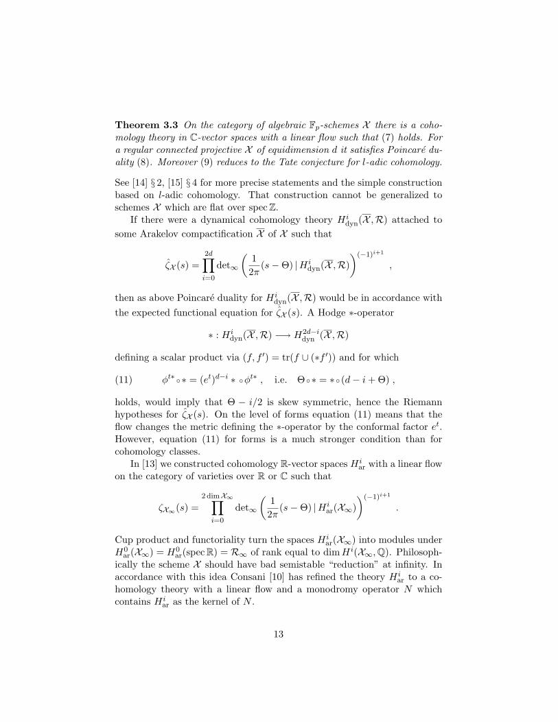
Theorem 3.3 On the category of algebraic Fp-schemes X there is a coho-mology theory in C-vector spaces with a linear flow such that (7) holds. Fora regular connected projective X of equidimension d it satisfies Poincare du-ality (8). Moreover (9) reduces to the Tate conjecture for l-adic cohomology.

See [14] § 2, [15] § 4 for more precise statements and the simple constructionbased on l-adic cohomology. That construction cannot be generalized toschemes X which are flat over spec Z.

If there were a dynamical cohomology theory H idyn(X ,R) attached to

some Arakelov compactification X of X such that

ζX (s) =2d∏i=0

det∞

(12π

(s−Θ) |H idyn(X ,R)

)(−1)i+1

,

then as above Poincare duality for H idyn(X ,R) would be in accordance with

the expected functional equation for ζX (s). A Hodge ∗-operator

∗ : H idyn(X ,R) −→ H2d−i

dyn (X ,R)

defining a scalar product via (f, f ′) = tr(f ∪ (∗f ′)) and for which

(11) φt∗ ∗ = (et)d−i ∗ φt∗ , i.e. Θ ∗ = ∗ (d− i+ Θ) ,

holds, would imply that Θ − i/2 is skew symmetric, hence the Riemannhypotheses for ζX (s). On the level of forms equation (11) means that theflow changes the metric defining the ∗-operator by the conformal factor et.However, equation (11) for forms is a much stronger condition than forcohomology classes.

In [13] we constructed cohomology R-vector spaces H iar with a linear flow

on the category of varieties over R or C such that

ζX∞(s) =2 dimX∞∏

i=0

det∞

(12π

(s−Θ) |H iar(X∞)

)(−1)i+1

.

Cup product and functoriality turn the spaces H iar(X∞) into modules under

H0ar(X∞) = H0

ar(spec R) = R∞ of rank equal to dimH i(X∞,Q). Philosoph-ically the scheme X should have bad semistable “reduction” at infinity. Inaccordance with this idea Consani [10] has refined the theory H i

ar to a co-homology theory with a linear flow and a monodromy operator N whichcontains H i

ar as the kernel of N .

13

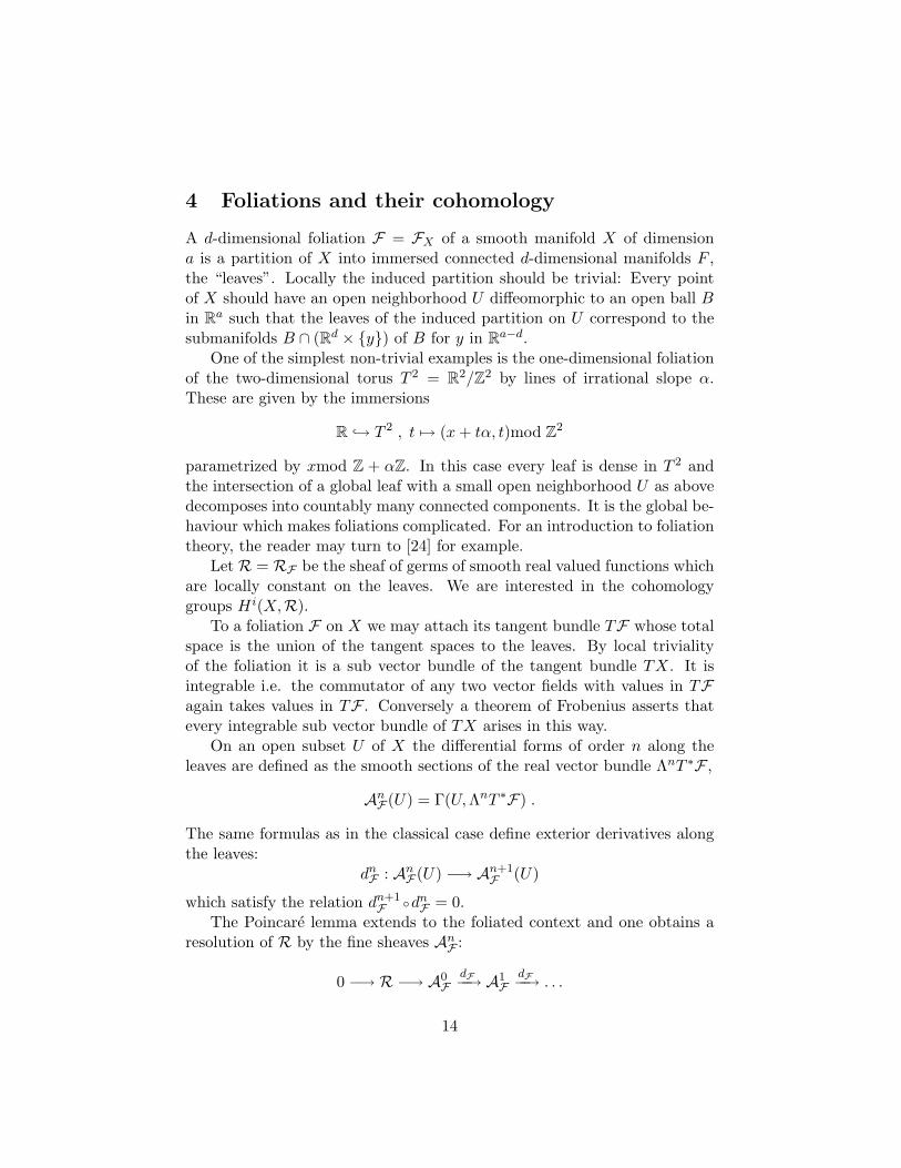
4 Foliations and their cohomology

A d-dimensional foliation F = FX of a smooth manifold X of dimensiona is a partition of X into immersed connected d-dimensional manifolds F ,the “leaves”. Locally the induced partition should be trivial: Every pointof X should have an open neighborhood U diffeomorphic to an open ball Bin Ra such that the leaves of the induced partition on U correspond to thesubmanifolds B ∩ (Rd × y) of B for y in Ra−d.

One of the simplest non-trivial examples is the one-dimensional foliationof the two-dimensional torus T 2 = R2/Z2 by lines of irrational slope α.These are given by the immersions

R → T 2 , t 7→ (x+ tα, t)mod Z2

parametrized by xmod Z + αZ. In this case every leaf is dense in T 2 andthe intersection of a global leaf with a small open neighborhood U as abovedecomposes into countably many connected components. It is the global be-haviour which makes foliations complicated. For an introduction to foliationtheory, the reader may turn to [24] for example.

Let R = RF be the sheaf of germs of smooth real valued functions whichare locally constant on the leaves. We are interested in the cohomologygroups H i(X,R).

To a foliation F on X we may attach its tangent bundle TF whose totalspace is the union of the tangent spaces to the leaves. By local trivialityof the foliation it is a sub vector bundle of the tangent bundle TX. It isintegrable i.e. the commutator of any two vector fields with values in TFagain takes values in TF . Conversely a theorem of Frobenius asserts thatevery integrable sub vector bundle of TX arises in this way.

On an open subset U of X the differential forms of order n along theleaves are defined as the smooth sections of the real vector bundle ΛnT ∗F ,

AnF (U) = Γ(U,ΛnT ∗F) .

The same formulas as in the classical case define exterior derivatives alongthe leaves:

dnF : An

F (U) −→ An+1F (U)

which satisfy the relation dn+1F dn

F = 0.The Poincare lemma extends to the foliated context and one obtains a

resolution of R by the fine sheaves AnF :

0 −→ R −→ A0F

dF−−→ A1F

dF−−→ . . .

14

Hence we have the following de Rham description of the cohomology of R:

Hn(X,R) = Ker (dnF : An

F (X)→ An+1F (X))/Im (dn−1

F : An−1F (X)→ An

F (X)) .

For our purposes these invariants are actually too subtle. We thereforeconsider the reduced leafwise cohomology

Hn(X,R) = Ker dnF/Im dn−1

F .

Here the quotient is taken with respect to the topological closure of Im dn−1F

in the natural Frechet topology on AnF (X). The reduced cohomologies are

nuclear Frechet spaces. Even if the leaves are dense, already H1(X,R) canbe infinite dimensional, c.f. [20].

The cup product pairing induced by the exterior product of forms alongthe leaves turns H•(X,R) into a graded commutative H0(X,R)-algebra.

For the torus foliation above with α /∈ Q we have H0(T 2,R) = R. SomeFourier analysis reveals that H1(T 2,R) ∼= R. The higher cohomologiesvanish since by the de Rham description we have

Hn(X,R) = 0 for all n > d = dimF .

For a smooth map f : X → Y of foliated manifolds which maps leaves intoleaves, continuous pullback maps

f∗ : AnFY

(Y ) −→ AnFX

(X)

are defined for all n. They commute with dF and respect the exterior prod-uct of forms. Hence they induce a continuous map of reduced cohomologyalgebras

f∗ : H•(Y,RY ) −→ H•(X,RX) .

A (complete) flow is a smooth R-action φ : R×X → X, (t, x) 7→ φt(x). It iscalled F-compatible if every diffeomorphism φt : X → X maps leaves intoleaves. If this is the case we obtain a linear R-action t 7→ φt∗ on Hn(X,R)for every n. Let

Θ : Hn(X,R) −→ Hn(X,R)

denote the infinitesimal generator of φt∗:

Θh = limt→0

1t(φt∗h− h) .

The limit exists and Θ is continuous in the Frechet topology. As φt∗ is analgebra endomorphism of the R-algebra H•(X,R) it follows that Θ is anR-linear derivation. Thus we have

(12) Θ(h1 ∪ h2) = Θh1 ∪ h2 + h1 ∪Θh2

15

for all h1, h2 in Hn(X,R).For arbitrary foliations the reduced leafwise cohomology does not seem

to have a good structure theory. For Riemannian foliations however thesituation is much better. These foliations are characterized by the existenceof a “bundle-like” metric g. This is a Riemannian metric whose geodesics areperpendicular to all leaves whenever they are perpendicular to one leaf. Forexample any one-codimensional foliation given by a closed one-form withoutsingularities is Riemannian.

Assuming that X is also oriented, the graded Frechet space A•F (X) car-ries a canonical inner product:

(α, β) =∫

X〈α, β〉Fvol .

Here 〈, 〉F is the Riemannian metric on Λ•T ∗F induced by g and vol is thevolume form or density on X coming from g. Let

∆F = dFd∗F + d∗FdF

denote the Laplacian using the formal adjoint of dF on X. Since F isRiemannian the restriction of ∆F to any leaf F is the Laplacian on F withrespect to the induced metric [1] Lemma 3.2, i.e.

(∆Fα) |F = ∆F (α |F ) for all α ∈ A•F (X) .

We now assume that also TF is orientable. Via g the choice of an orientationdetermines a volume form volF in Ad

F (X) and hence a Hodge ∗-operator

∗F : ΛnT ∗xF∼−→ Λd−nT ∗xF for every x in X .

It is determined by the condition that

v ∧ ∗Fw = 〈v, w〉F volF ,x for v, w in Λ•T ∗xF .

These fibrewise star-operators induce the leafwise ∗-operator on forms:

∗F : AnF (X) ∼−→ Ad−n

F (X) .

We now list some important properties of leafwise cohomology.Properties Assume that X is compact, F a d-dimensional oriented

Riemannian foliation and g a bundle-like metric for F .Then the natural map

(13) Ker∆nF∼−→ Hn(X,R) , ω 7−→ ω mod Im dn−1

F

16

is a topological isomorphism of Frechet spaces. We denote its inverse by H.This result is due to Alvarez Lopez and Kordyukov [1]. It is quite deep

since ∆F is only elliptic along the leaves so that the ordinary elliptic regu-larity theory does not suffice. For non-Riemannian foliations (13) does nothold in general [20]. All the following results are consquences of this Hodgetheorem.

The Hodge ∗-operator induces an isomorphism

∗F : Ker∆nF∼−→ Ker ∆d−n

F

since it commutes with ∆F up to sign. From (13) we therefore get isomor-phisms for all n:

(14) ∗F : Hn(X,R) ∼−→ Hd−n(X,R) .

For the next property define the trace map

tr : Hd(X,R) −→ R

by the formula

tr(h) =∫

X∗F (H(h))vol .

It is an isomorphism if F has a dense leaf. Note that for any representativeα in the cohomology class h we have

tr(h) =∫

X∗F (α)vol .

Namely α−H(h) = dFβ and∫X∗F (dFβ)vol = ±

∫Xd∗F (∗Fβ)vol

= ±(1, d∗F (∗Fβ))= ±(dF (1), ∗Fβ)= 0 .

It is not difficult to see using (13) that we get a scalar product on Hn(X,R)for every n by setting:

(h, h′) = tr(h ∪ ∗Fh′)(15)

=∫

X〈H(h),H(h′)〉Fvol .

17

It follows from this that the cup product pairing

(16) ∪ : Hn(X,R)× Hd−n(X,R) −→ Hd(X,R) tr−→ R

is non-degenerate.Next we discuss the Kunneth formula. Assume that Y is another com-

pact manifold with a Riemannian foliation. Then the canonical map

Hn(X,R)⊗Hm(Y,R) −→ Hn+m(X × Y,R)

induces a topological isomorphism [35]:

(17) Hn(X,R)⊗Hm(Y,R) ∼−→ Hn+m(X × Y,R) .

Since the reduced cohomology groups are nuclear Frechet spaces, it does notmatter which topological tensor product is chosen in (17). The proof of thisKunneth formula uses (13) and the spectral theory of the Laplacian ∆F .

Before we deal with more specific topics let us mention that Hodge–Kahler theory can also be generalized to the foliated context. A complexstructure on a foliation F is an almost complex structure J on TF suchthat all restrictions J |F to the leaves are integrable. Then the leaves carryholomorphic structures which vary smoothly in the transverse direction. Afoliation F with a complex structure J is called Kahler if there is a hermitianmetric h on the complex bundle TcF = (TF , J) such that the Kahler formalong the leaves

ωF = −12imh ∈ A2

F (X)

is closed. Note that for example any foliation by orientable surfaces can begiven a Kahlerian structure by choosing a metric on X, c.f. [33] LemmaA.3.1. Let

LF : Hn(X,R) −→ Hn+2(X,R) , LF (h) = h ∪ [ωF ]

denote the Lefschetz operator.The following assertions are consequences of (13) combined with the

classical Hodge–Kahler theory. See [22] for details. Let X be a compact ori-entable manifold and F a Kahlerian foliation with respect to the hermitianmetric h on TcF . Assume in addition that F is Riemannian. Then we have:

(18) Hn(X,R)⊗ C =⊕

p+q=n

Hpq , where Hpq = Hqp .

18

Here Hpq consists of those classes that can be represented by (p, q)-formsalong the leaves. Moreover there are topological isomorphisms

Hpq ∼= Hq(X,ΩpF )

with the reduced cohomology of the sheaf of holomorphic p-forms along theleaves.

Furthermore the Lefschetz operator induces isomorphisms

(19) LiF : Hd−i(X,R) ∼−→ Hd+i(X,R) for 0 ≤ i ≤ d .

Finally the space of primitive cohomology classes Hn(X,R)prim carries thestructure of a polarizable ind R-Hodge structure of weight n.

After this review of important properties of the reduced leafwise coho-mology of Riemannian foliations we turn to a specific result relating flowsand cohomology. This is a kind of toy model for the dynamical cohomologiesin the preceeding section. The existence of a conformal metric for the flowsimplifies the analysis. However, I do not think that such a metric will existfor dynamical systems relevant to number fields. In order to verify equation(11) for them one will need the Kahler identities on cohomology.

Theorem 4.1 Let X be a compact 3-manifold and F a Riemannian foli-ation by surfaces with a dense leaf. Let φt be an F-compatible flow on Xwhich is conformal on TF with respect to a metric g on TF in the sensethat for some constant α and all x ∈ X and t ∈ R we have:

(20) g(Txφt(v), Txφ

t(w)) = eαtg(v, w) for all v, w ∈ TxF .

Then we have for the infinitesimal generator of φt∗ that:

Θ = 0 on H0(X,R) = R and Θ = α on H2(X,R) ∼= R .

On H1(X,R) the operator Θ has the form

Θ =α

2+ S

where S is skew-symmetric with respect to the inner product (, ) above.

Remark For the bundle-like metric on X required for the construction of(, ) we take any extension of the given metric on TF to a bundle-like metricon TX. Such extensions exist.

19

Proof of 4.1 Because we have a dense leaf, H0(X,R) = H0(X,R) consistsonly of constant functions. On these φt∗ acts trivially so that Θ = 0. Since

∗F : R = H0(X,R) ∼−→ H2(X,R)

is an isomorphism and since

φt∗(∗F (1)) = eαt(∗F1)

by conformality, we have Θ = α on H2(X,R).For h1, h2 in H1(X,R) we find

(21) α(h1 ∪ h2) = Θ(h1 ∪ h2) = Θh1 ∪ h2 + h1 ∪Θh2 .

By conformality φt∗ commutes with ∗F on H1(X,R). Differentiating, itfollows that Θ commutes with ∗F as well. Since by definition we have

(h, h′) = tr(h ∪ ∗Fh′) for h, h′ ∈ H1(X,R) ,

it follows from (21) that as desired:

α(h, h′) = (Θh, h′) + (h,Θh′) .

2

5 Dynamical Lefschetz trace formulas

The formulas we want to consider in this section relate the compact orbitsof a flow with the alternating sum of suitable traces on cohomology. Asuggestive but non-rigorous argument of Guillemin [25] later rediscovered byPatterson [37] led to the following conjecture [16] § 3. Let X be a compactmanifold with a one-codimensional foliation F and an F-compatible flow φ.Assume that the fixed points and the periodic orbits of the flow are non-degenerate in the following sense: For any fixed point x and every t > 0, thetangent map Txφ

t has eigenvalues different from 1. For any closed orbit γ oflength l(γ) and any x ∈ γ and integer k 6= 0 the automorphism Txφ

kl(γ) ofTxX should have the eigenvalue 1 with algebraic multiplicity one. Observethat the vector field Yφ generated by the flow provides an eigenvector Yφ,x

for the eigenvalue 1.Recall that the length l(γ) > 0 of γ is defined by the isomorphism:

R/l(γ)Z ∼−→ γ , t 7−→ φt(x) .

20

For a fixed point x we set1

εx = sgn det(1− Txφt |TxF) .

This is independent of t > 0. For a closed orbit γ and k ∈ Z \ 0 set1

εγ(k) = sgn det(1− Txφkl(γ) |TxX/RYφ,x) .

It does not depend on the point x ∈ γ.Finally let D′(J) denote the space of Schwartz distributions on an open

subset J of R.

Conjecture 5.1 For X,F and φ as above there exists a natural definitionof a D′(R>0)-valued trace of φ∗ on the reduced leafwise cohomology H•(X,R)such that in D′(R>0) we have:(22)dimF∑n=0

(−1)nTr(φ∗ | Hn(X,R)) =∑

γ

l(γ)∞∑

k=1

εγ(k)δkl(γ) +∑

x

εx|1− eκxt|−1 .

Here γ runs over the closed orbits of φ which are not contained in a leafand x over the fixed points. For a ∈ R, δa is the Dirac distribution in aand κx is defined by the action of Txφ

t on the 1-dimensional vector spaceTxX/TxF . That action is multiplication by eκxt for some κx ∈ R and all t.

The conjecture is not known (except for dimX = 1) if φ has fixed points.It may well have to be amended somewhat in that case. The analytic dif-ficulty in the presence of fixed points lies in the fact that in this case ∆Fcannot be transversally elliptic to the R-action by the flow, so that themethods of transverse index theory do not apply directly. In the simplercase when the flow is everywhere transversal to F , Alvarez Lopez and Ko-rdyukov have proved a beautiful strengthening of the conjecture. Partialresults were obtained by other methods in [30], [21]. We now describe theirresult in a convenient way for our purposes:

5.2 Assume X is a compact oriented manifold with a one codimensionalfoliation F . Let φ be a flow on X which is everywhere transversal to theleaves of F . Then F inherits an orientation and it is Riemannian [24] III4.4. Fixing a bundle-like metric g, the cohomologies Hn(X,R) acquire pre-Hilbert structures (15) and we can consider their Hilbert space completionsHn(X,R). For every t the linear operator φt∗ is bounded on (Hn(X,R), ‖ ‖)and hence can be continued uniquely to a bounded operator on Hn(X,R)c.f. theorem 5.4.

1This is different from the normalization in [16] § 3.

21

By transversality the flow has no fixed points. We assume that all peri-odic orbits are non-degenerate.

Theorem 5.3 ([2]) Under the conditions of (5.2), for every test functionϕ ∈ D(R) = C∞0 (R) the operator

Aϕ =∫

Rϕ(t)φt∗ dt

on Hn(X,R) is of trace class. Setting:

Tr(φ∗ | Hn(X,R))(ϕ) = trAϕ

defines a distribution on R. The following formula holds in D′(R):(23)

dimF∑n=0

(−1)nTr(φ∗ | Hn(X,R)) = χCo(F , µ)δ0 +∑

γ

l(γ)∑

k∈Z\0

εγ(k)δkl(γ) .

Here χCo(F , µ) denotes Connes’ Euler characteristic of the foliation withrespect to the transverse measure µ corresponding to tr. (See [33].)

It follows from the theorem that if the right hand side of (23) is non-zero,at least one of the cohomology groups Hn

F (X) must be infinite dimensional.Otherwise the alternating sum of traces would be a smooth function andhence have empty singular support.

By the Hodge isomorphism (13) one may replace cohomology by thespaces of leafwise harmonic forms. The left hand side of the dynamicalLefschetz trace formula then becomes the D′(R)-valued transverse index ofthe leafwise de Rham complex. Note that the latter is transversely ellip-tic for the R-action φt. Transverse index theory with respect to compactgroup actions was initiated in [4]. A definition for non-compact groups of atransverse index was later given by Hormander [42] Appendix II.

As far as we know the relation of (23) with transverse index theory inthe sense of Connes–Moscovici still needs to be clarified.

Let us now make some remarks on the operators φt∗ on Hn(X,R) in amore general setting:

Theorem 5.4 Let F be a Riemannian foliation on a compact manifold Xand g a bundle like metric. As above Hn(X,R) denotes the Hilbert spacecompletion of Hn(X,R) with respect to the scalar product (15). Let φt bean F-compatible flow. Then the linear operators φt∗ on Hn(X,R) induce a

22

strongly continuous operator group on Hn(X,R). In particular the infinites-imal generator Θ exists as a closed densely defined operator. On Hn(X,R)it agrees with the infinitesimal generator in the Frechet topology defined ear-lier. There exists ω > 0 such that the spectrum of Θ lies in −ω ≤ Re s ≤ ω.If the operators φt∗ are orthogonal then T = −iΘ is a self-adjoint operatoron Hn(X,R)⊗ C and we have

φt∗ = exp tΘ = exp itT

in the sense of the functional calculus for (unbounded) self-adjoint operatorson Hilbert spaces.

Sketch of proof Estimates show that ‖φt∗‖ is locally uniformly boundedin t on Hn(X,R). Approximating h ∈ Hn(X,R) by hν ∈ Hn(X,R) onenow shows as in the proof of the Riemann–Lebesgue lemma that the func-tion t 7→ φt∗h is continuous at zero, hence everywhere. Thus φt∗ definesa strongly continuous group on Hn(X,R). The remaining assertions fol-low from semigroup theory [19], Ch. VIII, XII, and in particular from thetheorem of Stone.

We now combine theorems 4.1, 5.3 and 5.4 to obtain the following corol-lary:

Corollary 5.5 Let X be a compact 3-manifold with a foliation F by surfaceshaving a dense leaf. Let φt be a non-degenerate F-compatible flow which iseverywhere transversal to F . Assume that φt is conformal as in (20) withrespect to a metric g on TF . Then Θ has pure point spectrum Sp1(Θ) onH1(X,R) which is discrete in R and we have the following equalities ofdistributions on R:

2∑i=0

(−1)iTr(φ∗ | H i(X,R)) = 1−∑

ρ∈Sp1(Θ)

etρ + etα(24)

= χCo(F , µ)δ0 +∑

γ

l(γ)∑

k∈Z\0

εγ(k)δkl(γ) .

In the sum the ρ’s appear with their geometric multiplicities. All ρ ∈ Sp1(Θ)have Re ρ = α

2 .

Remarks 1) Here etρ, etα are viewed as distributions so that evaluatedon a test function ϕ ∈ D(R) the formula reads:(25)Φ(0)−

∑ρ∈Sp1(Θ)

Φ(ρ) + Φ(α) = χCo(F , µ)ϕ(0) +∑

γ

l(γ)∑

k∈Z\0

εγ(k)ϕ(kl(γ)) .

23

Here we have put

Φ(s) =∫

Retsϕ(t) dt .

2) Actually the conditions of the corollary force α = 0 i.e. the flow must beisometric with respect to g. We have chosen to leave the α in the fomulationsince there are good reasons to expect the corollary to generalize to moregeneral phase spaces X than manifolds, where α 6= 0 becomes possible i.e.to Sullivan’s generalized solenoids. More on this in the next section.3) One can show that the group generated by the lengths of closed orbits isa finitely generated subgroup of R under the assumptions of the corollary.In order to achieve an infinitely generated group the flow must have fixedpoints.

Proof of 5.5 By 4.1, 5.3 we only need to show the equation

(26) Tr(φt∗ | H1(X,R)) =∑

ρ∈Sp1(Θ)

etρ

and the assertions about the spectrum of Θ. As in the proof of 4.1 one seesthat on H1(X,R) we have

(φt∗h, φt∗h′) = eαt(h, h′) .

Hence e−α2

tφt∗ is orthogonal and by the theorem of Stone

T = −iS

is selfadjoint on H1(X,R)⊗ C, if Θ = α2 + S. Moreover

e−α2

tφt∗ = exp itT ,

so that

(27) φt∗ = exp tΘ .

In [21] proof of 2.6, for isometric flows the relation

−Θ2 = ∆1 |ker ∆1F

was shown. Using the spectral theory of the ordinary Laplacian ∆1 on 1-forms it follows that Θ has pure point spectrum with finite multiplicities on

24

H1(X,R) ∼= ker ∆1F and that Sp1(Θ) is discrete in R. Alternatively, without

knowing α = 0, that proof gives:

−(Θ− α

2

)2= ∆1 |ker∆1

F.

This also implies the assertion on the spectrum of Θ on H1(X,R). 2

Remarks a Writing the eigenvalues ρ of Θ on H1(X,R) in the formρ = α

2 + ir, the proof shows that the numbers r2 are contained in thespectrum of the ordinary Laplacian ∆1 = ∆1

g on 1-forms on X. Here g isany extension of the metric g on TF to a bundle-like metric on TX. Onemay wonder whether there is a corresponding statement for the zeroes ofζK(s): Are the squares of their imaginary parts contained in the spectrumof suitable Laplace–Bertrami operators on 1-forms?b In more general situations where Θ may not have a pure point spectrumon H1(X,R) but where e−

α2 φt∗ is still orthogonal, we obtain:

〈Tr(φ∗ | H1(X,R)), ϕ〉 =∑

ρ∈Sp1(Θ)point

Φ(ρ) +∫ α

2+i∞

α2−i∞

Φ(λ)m(λ) dλ

where m(λ) ≥ 0 is the spectral density function of the continuous part ofthe spectrum of Θ.

6 Comparison with the “explicit formulas” in an-alytic number theory

Consider a number field K/Q. Formula (22) restricted to R>0 implies thefollowing equality of distributions on R>0:

2∑i=0

(−1)iTr(φ∗ |H idyn(spec o,R)) = 1−

∑ζK(ρ)=0

etρ + et(28)

=∑p-∞

logNp

∞∑k=1

δk log Np +∑p |∞

(1− eκpt)−1 .

This fits rather nicely with formula (24) and suggests the following analogies:

25

spec oK ∪ p |∞ = 3-dimensional dynamical system (X,φt) witha one-codimensional foliation F satisfying theconditions of conjecture 5.1

finite place p = closed orbit γ = γp not contained in a leaf andhence transversal to F such that l(γp) = logNp

and εγp(k) = 1 for all k ≥ 1.infinite place p = fixed point xp such that κxp = κp and εxp = 1.H i

dyn(spec o,R) = H i(X,R)

In order to understand number theory more deeply in geometric termsit would be very desirable to find a system (X,φt,F) which actually re-alizes this correspondence. For this the class of compact 3-manifolds asphase spaces has to be generalized as will become clear from the followingdiscussion.

Let us compare formula (5) on all of R with formula (24) in Corollary5.5. This corollary is the best result yet on the dynamical side but still onlya first step since it does not allow for fixed points which as we have seenmust be expected for dynamical systems of relevance for number fields.

Ignoring the contributions Wp from the infinite places for the momentwe are suggested that

(29) − log |dK/Q| = χCo(F , µ) .

There are two nice points about this analogy. Firstly there is the followingwell known fact due to Connes:

Fact 6.1 Let F be a foliation of a compact 3-manifold by surfaces such thatthe union of the compact leaves has µ-measure zero, then

χCo(F , µ) ≤ 0 .

Namely the non-compact leaves are known to be complete in the inducedmetric. Hence they carry no non-zero harmonic L2-functions, so that Connes’0-th Betti number β0(F , µ) = 0. Since β2(F , µ) = β0(F , µ) it follows that

χCo(F , µ) = β0(F , µ)− β1(F , µ) + β2(F , µ)= −β1(F , µ) ≤ 0 .

The reader will have noticed that in accordance with 6.1 the left hand sideof (29) is negative as well:

− log |dK/Q| ≤ 0 for all K/Q .

26

The second nice point about (29) is this. The bundle-like metric g which wehave chosen for the definition of ∆F and of χCo(F , µ) induces a holomorphicstructure of F [33], Lemma A 3.1. The space X is therefore foliated byRiemann surfaces. Let χCo(F ,O, µ) denote the holomorphic Connes Eulercharacteristic of F defined using ∆∂-harmonic forms on the leaves instead of∆-harmonic ones. According to Connes’ Riemann–Roch Theorem [33] Cor.A. 2.3, Lemma A 3.3 we have:

χCo(F ,O, µ) =12χCo(F , µ) .

Therefore χCo(F ,O, µ) corresponds to − log√|dK/Q|.

Now, for completely different reasons this number is defined in Arakelovtheory as the Arakelov Euler characteristic of spec oK :

(30) χAr(Ospec oK) = − log

√|dK/Q| .

See [36] for example. Thus we see that

χAr(Ospec oK) corresponds to χCo(F ,O, µ) .

It would be very desirable of course to understand Arakelov Euler charac-teristics in higher dimensions even conjecturally in terms of Connes’ holo-morphic Euler characteristics. Note however that Connes’ Riemann–Rochtheorem in higher dimensions does not involve the R-genus appearing in theArakelov Riemann–Roch theorem. The ideas of Bismut [7] may be relevantin this connection. He interpretes the R-genus in a natural way via thegeometry of loop spaces.

Further comparison of formulas (5) and (24) shows that in a dynamicalsystem corresponding to number theory we must have α = 1. This meansthat the flow φt∗ would act by multiplication with et on the one-dimensionalspace H2

F (X). As explained before this would be the case if φt were confor-mal on TF with factor et:

(31) g(Txφt(v), Txφ

t(w)) = etg(v, w) for all v, w ∈ TxF .

However as mentioned before, this is not possible in the manifold setting ofcorollary 5.5 which actually implies α = 0.An equally important difference between formulas (5) and (24) is betweenthe coefficients of δkl(γ) and of δk log Np for k ≤ −1. In the first case it is ±1whereas in the second it is Npk = ek log Np which corresponds to ekl(γ).

27

Thus it becomes vital to find phase spaces X more general than mani-folds for which the analogue of corollary 5.5 holds and where α 6= 0 and inparticular α = 1 becomes possible. In the new context the term εγ(k)δkl(γ)

for k ≤ −1 in formula (24) should become εγ(k)eαkl(γ)δkl(γ). The next sec-tion is devoted to a discussion of certain laminated spaces which we proposeas possible candidates for this goal.

7 Remarks on dynamical Lefschetz trace formulason laminated spaces

In this section we extend the previous discussion to more general phasespaces than manifolds. The class of spaces we have in mind are the smoothsolenoids [45] or in other words foliated spaces with totally disconnectedtransversals in the sense of [33].

7.1 We start by recalling the definition of a foliated space with d-dimensionalleaves in the sense of [33] Cap. II. Consider a separable metrizable topo-logical space X with a covering by open sets Ui and homeomorphismsϕi : Ui → Fi × Ti with Fi open in Rd. This atlas should have the fol-lowing propertya The transition functions between different charts ϕi and ϕj have thefollowing form locally where x is the Euklidean and y the transversal coor-dinate

ϕj ϕ−1i (x, y) = (fij(x, y), gij(y)) .

b All partial derivatives Dαxfij(x, y) exist and are continuous as functions

of x and y.Two atlases of this kind are equivalent if their union is an atlas as well. A

foliated space with d-dimensional leaves is a space X as above together withan equivalence class of atlases. The coordinate change locally transformsthe level surface or plaque ϕ−1

i (Fi×y) to the level surface ϕ−1j (Fj ×y′)

where y′ = gij(y). Hence the level surfaces glue to maximal connected setswith a smooth d-dimensional manifold structure. These are the leaves Fof the foliated space X. Usually we indicate the foliated structure on atopological space X by another symbol, e.g. F which we also use to denotethe set of leaves.

A (generalized) solenoid of dimension a is a separable metrizable spaceX which is locally homeomorphic to a space of the form Li × Ti where Li

is an open subset of Ra and Ti is totally disconnected. For such spaces thetransition functions between charts automatically satisfy condition a since

28

continuous functions from connected subsets of Ra into a totally discon-nected space are constant. If X carries a smooth structure, i.e. if we aregiven an atlas of charts whose coordinate changes satisfy condition b, thenX becomes a foliated space with a-dimensional leaves. For this foliation Lthe leaves L of L are the path-connected components of X.

The two most prominent places in mathematics where (smooth) solenoidsoccur naturally are in number theory e.g. as adelic points of algebraic groupsand in the theory of dynamical systems as attractors.

The classical solenoid

S1p = R×Z Zp = lim←−(. . .

p−→ R/Z p−→ R/Z p−→ . . .)

is an example of a compact connected one-dimensional smooth solenoid withdense leaves diffeomorphic to the real line.

For a foliated space (X,F) let TF be the tangent bundle in the senseof [33] p. 43. For a point x ∈ X, the fibre TxF is the usual tangentspace of the leaf through the point x. Morphisms between foliated spacesare continuous maps which induce smooth maps between the leaves. Theyinduce morphisms of tangent bundles.

For a smooth solenoid (X,L) we set TX = TL. By definition, a Rie-mannian metric on X is one on TX.

7.2 We now turn to cohomology. For a foliated space (X,F) of leaf dimen-sion d consider the sheaf R = RF of real valued continuous functions whichare locally constant on the leaves. There is a natural de Rham resolution

0 −→ R −→ A0F

dF−−→ A1F

dF−−→ . . .

by the fine sheaves of differential forms along the leaves. Explicitly

AiF (U) = Γ(U,ΛiT ∗F)

for every open subset U of X. Here sections are by definition continuousand smooth on the leaves. Hence we have

H i(X,R) =Ker (dF : Ai

F (X)→ Ai+1F (X))

Im (dF : Ai−1F (X)→ Ai

F (X)).

As before, one also considers the maximal Hausdorff quotient H i(X,R) ofthis cohomology, obtained by dividing by the closure of Im dF in the naturalFrechet topology.

29

Warning A manifold with a (smooth) foliation is also a foliated space.However the sheaves R and Ai

F are different in the two contexts: In thefirst one demands smoothness also in the transversal direction whereas inthe second one only wants continuity.

Now consider an a-dimensional smooth solenoid (X,L) with a one-codi-mensional foliation F . By this we mean that X is equipped with a furtherstructure F of a foliated space, this time with leaves of dimension d = a− 1such that the leaves L of L are foliated by the leaves F of F with F ⊂ L.We denote by FL the induced one-codimensional foliation of L.

7.3 A flow φ on X is a continuous R-action such that the induced R-actionson the leaves of L are smooth. It is compatible with F if every φt mapsleaves of F into leaves of F . Thus (X,F , φt) is partitioned into the foliateddynamical systems (L,FL, φ

t |L) for L ∈ L. Any F-compatible flow φt

induces pullback actions φt∗ on H•(X,RF ) and H•(X,RF ).

7.4 We now state as a working hypotheses a generalization of the conjec-tured dynamical trace formula 5.1. We allow the phase space to be a smoothsolenoid. Moreover we extend the formula to an equality of distributions onR∗ instead of R>0. After checking various compatibilities we state a casewhere our working hypotheses can be proved and give a number theoreticalexample.

7.5 Working hypotheses: Let X be a compact smooth solenoid with aone-codimensional foliation F and an F-compatible flow φ. Assume that thefixed points and the periodic orbits of the flow are non-degenerate. Thenthere exists a natural definition of a D′(R∗)-valued trace of φt∗ on H•(X,R)where R = RF such that in D′(R∗) we have:

dimF∑n=0

(−1)nTr(φ∗ | Hn(X,R)) =(32)

∑γ

l(γ)

∑k≥1

εγ(k)δkl(γ) +∑

k≤−1

εγ(|k|) det(−Txφkl(γ) |TxF)δkl(γ)

+

∑x

Wx .

Here γ runs over the closed orbits not contained in a leaf and in the sumsover k’s any point x ∈ γ can be chosen. The second sum runs over the fixed

30

points x of the flow. The distributions Wx on R∗ are given by:

Wx |R>0 = εx |1− eκxt|−1

andWx |R<0 = εx det(−Txφ

t |TxF) |1− eκx|t||−1 .

Remarks 7.6 0) It may actually be better to use a version of foliationcohomology where transversally forms are only supposed to be locally L2

instead of being continuous. With such a foliation L2-cohomology, Leicht-nam [31] has proved certain fixed point free cases of the working hypothesisby generalizing the techniques of [1], [2] to the solenoidal setting.1) In the situation described in 7.7 below the working hypotheses can beproved, c.f. Theorem 7.8. In those cases there are no fixed points, onlyclosed orbits. Thus Theorem 7.8 dictated only the coefficients of δkl(γ) fork ∈ Z \ 0, but not the contributions Wx from the fixed points.2) The coefficients of δkl(γ) for k ∈ Z \ 0 can be written in a uniform way asfollows. They are equal to:

(33)det(1− Txφ

kl(γ) |TxF)|det(1− Txφ|k|l(γ) |TxX/RYφ,x)|

=det(1− Txφ

kl(γ) |TxF)|det(1− Txφ|k|l(γ) |TxF)|

.

Here x is any point on γ. Namely, for k ≥ 1 this equals εγ(k) whereas fork ≤ −1 we obtain

(34) εγ(|k|) det(−Txφkl(γ) |TxF) = εγ(k) |det(Txφ

kl(γ) |TxF)| .

The expression on the left hand side of (33) motivated our conjecture aboutthe contributions on R∗ from the fixed points x. Since Yφ,x = 0, they shouldbe given by:

det(1− Txφt |TxF)

|det(1− Txφ|t| |TxX)|!= Wx .

3) One can prove that in the manifold setting of theorem 5.3 we have

|det(Txφkl(γ) |TxF)| = 1 .

By (34), our working hypotheses 7.5 is therefore compatible with formula(23). Compatibility with conjecture 5.1 is clear.4) We will see below that in our new context metrics g on TF can exist forwhich the flow has the conformal behaviour (31). Assuming we are in sucha situation and that F is 2-dimensional, we have:

|det(Txφkl(γ) |TxF)| = ekl(γ) for x ∈ γ, k ∈ Z

31

and|det(Txφ

t |TxF)| = et for a fixed point x .

In the latter case, we even have by continuity:

det(Txφt |TxF) = et ,

the determinant being positive for t = 0. Hence by (34) the conjecturedformula (32) reads as follows in this case:

2∑n=0

(−1)nTr(φ∗ | Hn(X,R))(35)

=∑

γ

l(γ)

∑k≥1

εγ(k)δkl(γ) +∑

k≤−1

εγ(k)ekl(γ)δkl(γ)

+∑

x

Wx .

Here:Wx |R>0 = εx |1− eκxt|−1

andWx |R<0 = εxe

t |1− eκx|t||−1 .

This fits perfectly with the explicit formula (6) if all εγp(k) = 1 and εxp = 1.Namely if l(γp) = logNp for p -∞ and κxp = κp for p |∞, then we have:

ekl(γp) = ek log Np = Npk for finite places p

andWxp = Wp on R∗ for the infinite places p .

5) In the setting of the preceeding remark the automorphisms

e−k2l(γ)Txφ

kl(γ) of TxF for x ∈ γ

respectivelye−

t2Txφ

t of TxF for a fixed point x

are orthogonal automorphisms. For a real 2 × 2 orthogonal determinant Owith detO = −1 we have:

det(1− uO) = 1− u2 .

The condition εγ(k) = +1 therefore implies that det(Txφkl(γ) |TxF) is posi-

tive for k ≥ 1 and hence for all k ∈ Z. The converse is also true. For a fixed

32

point we have already seen directly that det(Txφt |TxF) is positive for all

t ∈ R. Hence we have the following information.Fact In the situation of the preceeding remark, εk(γ) = +1 for all k ∈

Z \ 0 if and only if on TxF we have:

Txφkl(γ) = e

k2l(γ) ·Ok for Ok ∈ SO(TxF) .

For fixed points, εx = 1 is automatic and we have:

Txφt = e

t2Ot for Ot ∈ SO(TxF) .

In the number theoretical case the eigenvalues of Txφlog Np on TxF for

x ∈ γp would therefore be complex conjugate numbers of absolute valueNp1/2. If they are real then Txφ

log Np would simply be mutliplication by±Np1/2. If not, the situation would be more interesting. Are the eigenvaluesWeil numbers (of weight 1)? If yes there would be some elliptic curve overoK/p involved by Tate–Honda theory.6) It would of course be very desirable to extend the hypotheses 7.5 to aconjectured equality of distributions on all of R. By theorem 5.3 we expectone contribution of the form

χCo(F , µ) · δ0 .

The analogy with number theory suggests that there will also be somewhatcomplicated contributions from the fixed points in terms of principal valueswhich are hard to guess at the moment. After all, even the simpler conjecture5.1 has not yet been verified in the presence of fixed points!7) If there does exist a foliated dynamical system attached to spec oK withthe properties dictated by our considerations we would expect in particularthat for a preferred transverse measure µ we have:

χCo(F , µ) = − log |dK/Q| .

This gives some information on the space X with its F-foliation. If K/Q isramified at some finite place i.e. if dK/Q 6= ±1 then χCo(F , µ) < 0. Now,since H2(X,F) must be one-dimensional, it follows that

χCo(F , ν) < 0 for all non-trivial transverse measures ν .

Hence by a result of Candel [9] there is a Riemannian metric on TF , suchthat every F-leaf has constant curvature −1. Moreover (X,F) is isomorphicto

O(H,X)/PSO(2) .

33

Here O(H,X) is the space of conformal covering maps u : H → N as Nruns through the leaves of F with the compact open topology. See [9] fordetails.

In the unramified case, |dK/Q| = 1 we must have χCo(F , ν) = 0 for alltransverse measures by the above argument. Hence there is an F-leaf whichis either a plane, a torus or a cylinder c.f. [9].

7.7 In this final section we describe a simple case where the working hy-pothesis 7.5 can be proved.

Consider an unramified covering f : M → M of a compact connectedorientable d-dimensional manifold M . We set

M = lim←

(. . .f−→M

f−→M → . . .) .

Then M is a compact topological space equipped with the shift automor-phism f induced by f . It can be given the structure of a smooth solenoidas follows. Let M be the universal covering of M . For i ∈ Z there exists aGalois covering

pi : M −→M

with Galois group Γi such that pi = pi+1 f for all i. Hence we have inclu-sions:

. . . ⊂ Γi+1 ⊂ Γi ⊂ . . . ⊂ Γ0 =: Γ ∼= π1(M,x0) .

Writing the operation of Γ on X from the right, we get commutative dia-grams for i ≥ 0:

M ×Γ (Γ/Γi+1) M/Γi+1

pi+1∼−−−−→ Myid×proj

yproj

yf

M ×Γ (Γ/Γi) M/Γi

pi∼−−−−→ M

It follows that

(36) M ×Γ Γ ∼−→ M

where Γ is the pro-finite set with Γ-operation:

Γ = lim←

Γ/Γi .

The isomorphism (36) induces on M the structure of a smooth solenoid withrespect to which f becomes leafwise smooth.

34

Fix a positive number l > 0 and let Λ = lZ ⊂ R act on M as follows:λ = lν acts by fν . Define a right action of Λ on M × R by the formula

(m, t) · λ = (−λ ·m, t+ λ) = (f−λ/l(m), t+ λ) .

The suspension:X = M ×Λ R = (M ×Γ Γ)×Λ R

is an a = d + 1-dimensional smooth solenoid with a one-codimensional fo-liation F as in 7.2. The leaves of F are the images in X of the manifoldsM × γ × t for γ ∈ Γ and t ∈ R. Translation in the R-variable

φt[m, t′] = [m, t+ t′]

defines an F-compatible flow φ on X which is everywhere transverse to theleaves of F and in particular has no fixed points.

The mapγ 7−→ γM = γ ∩ (M ×Λ Λ)

gives a bijection between the closed orbits γ of the flow on X and the finiteorbits γM of the f - or Λ-action. These in turn are in bijection with the finiteorbits of the original f -action on M . We have:

l(γ) = |γM |l .

Theorem 7.8 In the situation of 7.7 assume that all periodic orbits of φare non-degenerate. Let Spn(Θ) denote the set of eigenvalues with theiralgebraic multiplicities of the infinitesimal generator Θ of φt∗ on Hn(X,R).Then the trace

Tr(φ∗ | Hn(X,R)) :=∑

λ∈Spn(Θ)

etΘ

defines a distribution on R and the following formula holds true in D′(R):

dimF∑n=0

(−1)nTr(φ∗ | Hn(X,R)) = χCo(F , µ) · δ0 +

∑γ

l(γ)

∑k≥1

εγ(k)δkl(γ) +∑

k≤−1

εγ(|k|) det(−Txφkl(γ) |TxF)δkl(γ)

.

Here γ runs over the closed orbits of φ and in the sum over k’s any pointx ∈ γ can be chosen. Moreover χCo(F , µ) is the Connes’ Euler characteristicof F with respect to a certain canonical transverse measure µ. Finally wehave the formula:

χCo(F , µ) = χ(M) · l .

35

A more general result is proved in [31].

Example Let E/Fp be an ordinary elliptic curve over Fp and let C/Γ be alift of E to a complex elliptic curve with CM by the ring of integers oK inan imaginary quadratic field K. Assume that the Frobenius endomorphismof E corresponds to the prime element π in oK . Then π is split, ππ = p andfor any embedding Ql ⊂ C, l 6= p the pairs

(H∗et(E ⊗ Fp,Ql)⊗ C,Frob∗) and (H∗(C/Γ,C), π∗)

are isomorphic. Setting M = C/Γ, f = π we are in the situation of 7.7 andwe find:

X = (C×Γ TπΓ)×Λ R .

HereTπΓ = lim

←Γ/πiΓ ∼= Zp

is the π-adic Tate module of C/Γ. It is isomorphic to the p-adic Tate moduleof E.

Setting l = log p, so that Λ = (log p)Z and passing to multiplicative time,X becomes isomorphic to

X ∼= (C×Γ TπΓ)×pZ R∗+

which may be a more natural way to write X. Note that pν acts on C×ΓTπΓby diagonal multiplication with πν . It turns out that the right hand side ofthe dynamical Lefschetz trace formula established in theorem 7.8 equals theright hand side in the explicit formulas for ζE(s). Moreover the metric g onTF given by

g[z,y,t](ξ, η) = etRe (ξη) for [z, y, t] in (C×Γ TπΓ)×Λ R

satisfies the conformality condition (20) for α = 1. The construction of(X,φt) that we made for ordinary elliptic curves is misleading however,since it almost never happens that a variety in characteristic p can be liftedto characteristic zero together with its Frobenius endomorphism.

Our present dream for the general situation is this: To an algebraicscheme X/Z one should first attach an infinite dimensional dissipative dy-namical system, possibly using GL∞ in some way. The desired dynamicalsystem should then be obtained by passing to the finite dimensional compactglobal attractor, c.f. [29] Part I.

36

8 Arithmetic topology and dynamical systems

In the sixties Mazur and Manin pointed out intriguing analogies betweenprime ideals in number rings and knots in 3-manifolds. Let us recall someof the relevant ideas.

In many respects the spectrum of a finite field Fq behaves like a topo-logical circle. For example its etale cohomology with Zl-coefficients for l - qis isomorphic to Zl in degrees 0 and 1 and it vanishes in higher degrees.

Artin and Verdier [3] have defined an etale topology on spec Z =spec Z ∪ ∞. In this topology spec Z has cohomological dimension three,up to 2-torsion.

The product formula ∏p≤∞|a|p = 1 for a ∈ Q∗ ,

allows one to view spec Z as a compact space: Namely in the function fieldcase the analogue of the product formula is equivalent to the formula∑

x

ordxf = 0

on a proper curve X0/Fq. Here x runs over the closed points of X0 andf ∈ Fq(X0)∗.

By a theorem of Minkowski there are no non-trivial extensions of Qunramified at all places p ≤ ∞. Thus

π1(spec Z) = 0 .

Hence, by analogy with the Poincare conjecture, Mazur suggested to thinkof spec Z as an arithmetic analogue of the 3-sphere S3. Under this analogythe inclusion:

spec Fp → spec Z

corresponds to an embedded circle i.e. to a knot.The analogue of the Alexander polynomial of a knot turns out to be

the Iwasawa zeta function. One can make this precise using p-adic etalecohomology for schemes over spec Z(p).

More generally, for a number field K consider

spec oK = spec oK ∪ p |∞

37

together with its Artin–Verdier etale topology. Via the inclusion

spec oK/p → spec oK

we may imagine a prime ideal p as being analogous to a knot in a compact3-manifold.

This nice analogy between number theory and three dimensional topol-ogy was further extended by Reznikov and Kapranov and baptized Arith-metic Topology. The reader may find dictionaries between the two fields in[39] and [41]. Further analogies were contributed in [34] and [38] for exam-ple. In particular Ramachandran had the idea that the infinite primes ofa number field should correspond to the ends of a non-compact manifold –the analogue of spec oK .

The arguments in the preceeding sections also lead to the idea that primeideals p in oK are knots in a 3-space. Namely, as we have seen a phase space(spec oK)dyn corresponding to spec oK would be three dimensional. Afterforgetting the parametrization of the periodic orbits the prime ideals canthus be viewed as knots in a 3-space.

It appears that the (sheaf) cohomology of (spec oK)dyn with constantcoefficients should play the role of an arithmetic as opposed to geometriccohomology theory for spec oK . In particular it would have cohomologicaldimension three. We wish to compare this as yet speculative theory with thel-adic cohomology of spec oK . More precisely we compare Lefschetz numbersof certain endomorphisms on these cohomologies.

In order to do this we first calculate the Lefschetz number of an auto-morphism σ of K on the Artin–Verdier etale cohomology of spec oK .

Next we prove a generalization of Hopf’s formula to a formula for theLefschetz number of an endomorphism of a dynamical system on a manifold.

Assuming our formula applies to ((spec oK)dyn, φt) we then obtain an ex-

pression for the Lefschetz number of the automorphism on H•dyn(spec oK ,R)

induced by σ.As it turns out, the two kinds of Lefschetz numbers agree in all cases,

even when generalized to constructible sheaf coefficients. This result wasprompted by a question of B. Mazur on the significance of etale Euler char-acteristics [12] in our dynamical picture.

We first recall a version of etale cohomology with compact supports ofarithmetic schemes that takes into account the fibres at infinity. Using thistheory we reformulate the main result of [12] on l-adic Lefschetz numbersof l-adic sheaves on arithmetic schemes as a vanishing statement. Thisformulation was suggested by Faltings [23] in his review of [12]. We alsocalculate l-adic Lefschetz numbers on arithmetically compactified schemes.

38

Let the scheme U/Z be algebraic i.e. separated and of finite type andset U∞ = Uan

C /GR where UC = U ⊗Z C and the Galois group GR of R actson Uan

C by complex conjugation. We give U∞ the quotient topology of UanC .

Artin and Verdier [3] define the etale topology on U = UqU∞ as follows.The category of “open sets” has objects the pairs(f : U ′ → U , D′) where f is an etale morphism and D′ ⊂ U ′∞ is open. Themap f∞ : D′ → U∞ induced by f is supposed to be “unramified” in thesense that f∞(D′) ∈ U(R) if and only if D′ ∈ U ′(R). Note that U(R) is aclosed subset of U∞.

A morphism

(f : U ′ → U , D′) −→ (g : U ′′ → U , D′′)

is a map U ′ → U ′′ commuting with the structure maps and such that theinduced map U ′∞ → U ′′∞ carries D′ into D′′. Coverings are the obvious ones.

Pullback defines morphisms of sites:

Uetj−→ U et

i←− U∞ .

Let ∼ denote the corresponding categories of abelian sheaves. One provesthat U∼et is the mapping cone of the left exact functor

i∗j∗ : Uet −→ U∞ .

In particular we have maps i! and j! at our disposal. Let us describe thefunctor i∗j∗ explicitely. Let α : Uan

C → Uet be the canonical map of sites.Note that α∗F is aGR-sheaf on Uan

C for every sheaf F on Uet. If π : UanC → U∞

denotes the natural projection, define the left exact functor

πGR∗ : (abelian GR-sheaves on Uan

C ) −→ U∞

byπGR∗ (G)(V ) = G(π−1(V ))GR .

Then one can check thati∗j∗ = πGR

∗ α∗ .

In particular we see that

i∗Rnj∗ = RnπGR∗ α∗ .

It follows that for n ≥ 1 the sheaf Rnj∗F = i∗i∗Rnj∗F is 2-torsion with

support on U(R) ⊂ U∞ as stated in [3]. In particular

(37) Hnet(U , j∗F ) −→ Hn

et(U , Rj∗F ) = Hnet(U , F )

39

is an isomorphism up to 2-torsion for n ≥ 1 (and an isomorphism for n = 0).Let us now define cohomology with compact supports for schemes X

which are proper over spec Z. We define:

Hnc (X , F ) := Hn(X , j!F ) .

The distinguished triangle

j!j∗G• −→ G• −→ i∗i

∗G• −→ . . .

for complexes of sheaves G• on X applied to G• = Rj∗F gives the triangle

j!F −→ Rj∗F −→ i∗i∗Rj∗F −→ . . .

From this one gets an exact sequence

−→ Hnc (X , F ) −→ Hn(X , F ) −→ Hn(X∞, i∗Rj∗F ) −→ . . .

We have i∗Rj∗ = RπGR∗ α∗ and

Hn(X∞, i∗Rj∗F ) = Hn(X∞, RπGR∗ (α∗F ))

= Hn(GR, RΓ(X anC , α∗F ))

= Hn(X anR , α∗F ) .(38)

Here, for any GR-sheaf G on a complex analytic space Y with a real structurewe set:

Hn(YR, G) = Hn(GR, RΓ(Y,G)) .

In conclusion we get the long exact sequence:

−→ Hnc (X , F ) −→ Hn(X , F ) −→ Hn(X an

R , α∗F ) −→ . . .

An endomorphism (σ, e) of the pair (X , F ) is a morphism σ : X → Xtogether with a homomorphism e : σ∗F → F of Ql-sheaves. It inducespullback endomorphisms on Hn

c (X , F ) and Hn(X , F ) and on Hnc (X an

R , α∗F ).For an endomorphism ϕ of a finite dimensional graded vector space H• wewill abbreviate the Lefschetz number as follows:

Tr(ϕ |H•) :=∑

i

(−1)iTr(ϕ |H i) .

The following theorem is a reformulation of results in [12]. They are basedon algebraic number theory and in particular on class field theory.

40

Theorem 8.1 Let (σ, e) be an endomorphism of (X , F ) as above, l 6= 2.The cohomologies H•

c (X , F ) and H•(X , F ) are finite dimensional and wehave:

(39) Tr((σ, e)∗ |H•c (X , F )) = 0 .

Furthermore we have

(40) Tr((σ, e)∗ |H•(X , j∗F )) = Tr((σ, e)∗ |H•(X anR , α∗F )) .

If in addition X is generically smooth and the fixed points x of σ on X∞ arenon-degenerate in the sense that det(1 − Txσ |Tx(X ⊗ R)) is non-zero thenwe have:

(41) Tr((σ, e)∗ |H•(X , j∗F )) =∑

x∈X∞σx=x

Tr(ex | (α∗F )x)εx(σ) .

Hereεx(σ) = sgn det(1− Txσ |Tx(X ⊗ R)) .

The following assertion is an immediate consequence of the theorem.

Corollary 8.2 Let σ be an endomorphism of a scheme X proper over spec Z.Then we have for any l 6= 2:

(42) Tr(σ∗ |H•c (X ,Ql)) = 0

and

(43) χ(H•(X , j∗Ql)) = χ(H•(X anR ,Ql)) .

If in addition X has a smooth generic fibre and the fixed points of σ on X∞are non-degenerate we have:

(44) Tr(σ∗ |H•(X , j∗Ql)) =∑

x∈X∞σx=x

εx(σ) .

8.3 We now explain analogies and an interesting difference with the caseof varieties over finite fields. For a variety X/Fq with an endomorphism σof X over Fq and a constructible Ql-sheaf F on X with an endomorphisme : σ∗F → F we have

(45) Tr((σ, e)∗ |H•c (X,F )) = 0

41

and

(46) Tr((σ, e)∗ |H•(X,F )) = 0 .

Contrary to the number field case these assertions are easy to prove. E.g.for the first one, set X = X ⊗ Fq, F = F |X . The Hochschild–Serre spectralsequence degenerates into short exact sequences:

0 −→ H1(Fq,Hn−1c (X,F )) −→ Hn

c (X,F ) −→ H0(Fq,Hnc (X,F )) −→ 0 .

Moreover for every GFq -module M there is an exact sequence:

0 −→ H0(Fq,M) −→M1−ϕ−−→M −→ H1(Fq,M) −→ 0

where ϕ is a generator of GFq . This implies (45) and (46) follows similarlysince all groups are known to be finite dimensional.

Now in the number field case, according to Theorem 8.1 (39) the analogueof (45) is valid. In particular, for any finite set S of prime ideals in ok wehave

(47) χ(H•c (spec oK,S ,Ql)) = 0 .

The analogue of (46) however is not valid in general: From Theorem 8.1(40) it follows for example that

(48) χ(H•(spec oK , j∗Ql) = number of infinite places of K .

The fact, that in (47) the Euler characteristic is unchanged if we increase Si.e. take out more finite places p follows directly from the fact that

χ(H•(spec (oK/p),Ql)) = 0 .

The topological intuition behind this equation is that finite primes are likecircles (whose Euler characteristic also vanishes). The difference between(47) and (48) comes from the different nature of the infinite places. Coho-mologically the complex places behave like points and the real places behavelike the “quotient of a point by GR”.

8.4 In this section we prove a formula for Lefschetz numbers of finite orderautomorphisms of dynamical systems. We also allow certain constructiblesheaves as coefficients.

42

Let us consider a complete flow φt on a compact manifold X. Assumethat for every fixed point x there is some δx > 0 such that

det(1− Txφt |TxX) 6= 0 for 0 < t < δx .

This condition is weaker than non-degeneracy. Still it implies that the fixedpoints are isolated and hence finite in number.

We also assume that the lengths of the closed orbits are bounded belowby some ε > 0.

Let σ be an automorphism of finite order of X which commutes with allφt i.e. an automorphism of (X,φ). Consider a constructible sheaf of Q - or R-vector spaces on X together with an endomorphism e : σ−1F → F . We alsoassume that there is an action ψt over φt i.e. isomorphisms ψt : (φt)−1F → Ffor all t satisfying the relations

ψ0 = id and ψt1+t2 = ψt2 (φt2)−1(ψt1) for all t1, t2 ∈ R .

For constant F there is a canonical action ψ.Note that σ and e determine an endomorphism (σ, e)∗ of H•(X,F ).Let us say that a point x ∈ X is φ-fix if φt(x) = x for all t ∈ R.

Then we have the following formula:

Theorem 8.5 Tr((σ, e)∗ |H•(X,F )) =∑

x∈X,φ−fixσx=x

Tr(ex |Fx)εx(σ)

whereεx(σ) = lim

t→0t>0

sgn det(1− Tx(φtσ) |TxX) .

Proof Assume N ≥ 1 is such that σN = 1 and fix some s with0 < s < N−1 minx∈X,φ−fix(ε, δx). If x is any point of X with (φsσ)(x) = x,then (φNsσN )(x) = x and hence φNs(x) = x. If x lay on a periodic orbit γthen l(γ) ≤ Ns and hence ε ≤ Ns contrary to the choice of s. Thus x isa fixed point of φ. Because of φs(x) = x we have σx = x as well. If 1 isan eigenvalue of Tx(φtσ) then 1 is an eigenvalue of (Tx(φtσ))N = Txφ

Nt aswell. Thus Nt ≥ δx. By assumption on s we have Ns < δx and therefore

det(1− Tx(φsσ) |TxX) 6= 0 .

In conclusion: the fixed points of the automorphism φsσ coincide with thosefixed points of the flow φ which are also kept fixed by σ. They are allnon-degenerate.

43

Consider the morphisms for t ∈ R

et = e σ−1(ψt) : (φtσ)−1F −→ F .

The Lefschetz fixed point formula for the endomorphism (φsσ, es) of (X,F )for a fixed s as above now gives the formula:

Tr((φsσ, es)∗ |H•(X,F )) =∑

x∈X,φ−fixσx=x

Tr((es)x |Fx)sgn det(1−Tx(φsσ) |TxX) .

The left hand side is defined for all s in R and by homotopy invariance ofcohomology it is independent of s. Passing to the limit s→ 0 for positive sin the formula thus gives the assertion. 2

Corollary 8.6 Let (X,φt, σ) be as in theorem 8.5 and let U ⊂ X be open,φ- and σ-invariant. Assume that X \ U is a compact submanifold of X.Consider a constructible sheaf F of Q- or R-vector spaces on U with anendomorphism e : σ−1F → F and an action ψt over φt |U . Then we have:

Tr((σ, e)∗ |H•c (U,F )) =

∑x∈U,φ−fix

σx=x

Tr(ex |Fx)εx(σ) .

In particularTr((σ, e)∗ |H•

c (U,F )) = 0

if φ has no fixed points on U .

Proof Apply 8.5 to (X, j!F ), where j : U → X is the inclusion. 2

8.7 We now compare arithmetic and dynamic Lefschetz numbers. Thissection is of a heuristic nature: we assume that a functor U 7→ (Udyn, φ

t)from flat algebraic schemes over spec Z to dynamical systems exists, withproperties as described before. We consider various cases.

2.7.1 Let σ be a finite order automorphism of a scheme X proper and flatover spec Z. The induced automorphism σ of Xdyn is an automorphism of(Xdyn, φ

t) and hence commutes with each φt. As we have seen, the phasespace Xdyn cannot be a manifold. Still let us assume that the assertion ofcorollary 8.6 applies to

(U, φt, σ, F, e, ψt) = (Xdyn, φt, σ,Q, id, id) .

44

Then we findTr(σ∗ |H•

c (Xdyn,Q)) = 0

in accordance with formula (42) since φt should have no fixed points onXdyn.

2.7.2 Now consider the case where in addition X has a smooth generic fibreand the fixed points of σ on X∞ are non-degenerate. Under assumptions asabove, from corollary 8.6 applied to

(U, φt, σ, F, e, ψt) = (X dyn, φt, σ, j∗Q, id, id)

we would get a formula corresponding to (44):

(49) Tr(σ∗ |H•(X dyn, j∗Q)) =∑

x∈X∞σx=x

εx(σ) .

Here we have used that the fixed point set of φt on X dyn should be X (C)/GR =X∞. Namely, in the case of X = spec oK , this is the set of archimedean val-uations of K. For general X we only have the following argument: The setof closed points of X over p can be identified with the set X (Fp)/〈Frp〉 ofFrobenius orbits on X (Fp). Thus the set of closed orbits of (Xdyn, φ

t) wouldbe in bijection with the union of all X (Fp)/〈Frp〉. Correspondingly it looksnatural to assume that the set of fixed points of φ would be in bijection withX (C)/〈F∞〉 = X∞ where the infinite Frobenius F∞ : X (C)→ X (C) acts bycomplex conjugation.

Actually the comparison of formulas (43) and (49) lends further credi-bility to this idea.

The different definitions of εx(σ) in (43) and (49) should agree.

References

[1] J.A. Alvarez Lopez, Y. Kordyukov, Long time behaviour of leafwiseheat flow for Riemannian foliations. Compositio Math. 125 (2001), 129–153

[2] J. Alvarez Lopez, Y. Kordyukov, Distributional Betti numbers of tran-sitive foliations of codimension one. Preprint 2000

[3] M. Artin, J-L. Verdier, Seminar on etale cohomology of number fields,Woods hole 1964

[4] M.F. Atiyah, Elliptic operators and compact groups. Springer LNM401, 1974

45

[5] K. Barner, On A. Weil’s explicit formula. J. Reine Angew. Math. 323(1981), 139–152

[6] M. Berry, Riemann’s zeta function: a model of quantum chaos, LectureNotes in Physics 263, Springer 1986

[7] J.-M. Bismut, Complex equivariant intersection, excess normal bundlesand Bott–Chern currents. Comm. Math. Phys. 148 (1992), 1–55

[8] S. Bloch, K. Kato, L-functions and Tamagawa numbers of motives.(Grothendieck Festschrift I) 333–400, Birkhauser 1991

[9] A. Candel, Uniformization of surface laminations. Ann. scient. Ec.Norm. Sup. 4e serie 26 (1993), 489–516

[10] K. Consani, Double complexes and Euler L-factors, Compos. Math. 111(1998), 323–358

[11] P. Deligne, La conjecture de Weil I. Inst. Hautes Etudes Sci. Publ.Math. 43 (1974), 273–307

[12] C. Deninger, l–adic Lefschetz numbers of arithmetical schemes. J. ReineAngew. Math. 375/376 (1987), 326–345

[13] C. Deninger, On the Γ-factors attached to motives. Invent. Math. 104(1991), 245–261

[14] C. Deninger, Local L-factors of motives and regularized determinants.Invent. Math. 107 (1992), 135–150

[15] C. Deninger, Motivic L–functions and regularized determinants. Proc.Symp. Pure Math. 55, 1 (1994), 707–743

[16] C. Deninger, Some analogies between number theory and dynamicalsystems on foliated spaces. Doc. Math. J. DMV. Extra Volume ICM I(1998), 23–46

[17] C. Deninger, Number theory and dynamical systems on foliated spaces.Jber. d. Dt. Math.-Verein. 103 (2001), 79–100

[18] C. Deninger, A note on arithmetical topology and dynamical systems.In: S. Vostokov, Y. Zarhin (eds.), Algebraic Number Theory and Alge-braic Geometry. Papers Dedicated to A.N. Parshin on the Occasion ofhis Sixtieth Birthday. Contemporary Mathematics 300 (2002), 99–114

[19] C. Deninger, M. Schroter, A distribution theoretic interpretation ofGuinand’s functional equation for Cramer’s V –function and general-izations. J. London Math. Soc. (2) 52 (1995) 48–60

[20] C. Deninger, W. Singhof, A counterexample to smooth leafwise Hodgedecomposition for general foliations and to a type of dynamical traceformulas. Ann. Int. Fourier, Grenoble, 51, 1 (2001), 209–219

[21] C. Deninger, W. Singhof, A note on dynamical trace formulas. To ap-pear in a proceedings volume on dynamical systems edited by M.L.Lapidus, M. van Frankenhuysen

46

[22] C. Deninger, W. Singhof, Real polarizable Hodge structures arisingfrom foliations. Annals of Global Analysis and Geometry 21 (2002),377–399

[23] G. Faltings, Review of [12] in Mathematical Reviews 88 f: 14017 (1988)[24] C. Godbillon, Feuilletages. Progress in Math. 98, Birkhauser 1991[25] V. Guillemin, Lectures on spectral theory of elliptic operators. Duke

Math. J. 44 (1977), 485–517[26] G. Illies, Regularized products and determinants. Comm. Math. Phys.

220 (2001), 69–94[27] J. Jorgenson, S. Lang, Explicit formulas and regularized products, Lec-

ture Notes in Mathematics 1593, Springer 1994[28] N. Kurokawa, Parabolic components of zeta function. Proc. Japan

Acad. Ser. A64 (1988) 21–24[29] O. Ladyzhenskaya, Attractors for semigroups and evolution equations.

Cambridge university press 1991[30] C. Lazarov, Transverse index and periodic orbits. GAFA 10 (2000),

124–159[31] E. Leichtnam, Renormalization group flow and arithmetic zeta func-

tions I. Preprint in preparation[32] S. Lichtenbaum, The Weil-etale topology for number rings. Preprint

2005. ArXiv math.AG/0503604[33] C.C. Moore, C. Schochet, Global analysis on foliated spaces. MSRI

Publications 9, Springer 1988[34] M. Morishita, On certain analogies between knots and primes. J. reine

Angew. Math. 550 (2002), 141–167[35] B. Mumken, A coincidence formula for foliated manifolds. Preprint

2003. ArXiv math. GT/0306031[36] J. Neukirch, Algebraic number theory. Springer Grundlehren 322, 1999[37] S.J. Patterson, On Ruelle’s zeta function. Israel Math. Conf. Proc. 3

(1990), 163–184[38] N. Ramachandran, A note on arithmetic topology. Preprint 2001[39] A. Reznikov, Embedded incompressible surfaces and homology of ram-

ified coverings of three-manifolds. Sel. math., New series 6 (2000), 1–39[40] P. Sarnak, Quantum Chaos, Symmetry and Zeta Functions, Lecture I:

Quantum Chaos, Lecture II: Zeta Functions, Curr. Dev. Math. 84–115,International Press 1997

[41] A.S. Sikora, Analogies between group actions on 3-manifolds and num-ber fields. Preprint arXiv: math.GT/0107210, 29. Juli 2001

47

[42] I.M. Singer, Index theory for elliptic operators, Proc. Symp. Pure Math.28 (1973), 11–31

[43] C. Soule, Sur les zeros des fonctions L automorphes. CR Acad. Sci.Paris Ser. I Math. 328 (1999), 955–958

[44] M. Schroter, C. Soule, On a result of Deninger concerning Riemann’szeta function, Proc. Sympos. Pure Math. 55 (1994), 745–747

[45] D. Sullivan, Linking the universalities of Milnor–Thurston Feigenbaumand Ahlfors-Bers. In: Topological methods in modern mathematics.Publish or Perish 1993, pp. 543–564.

Mathematisches InstitutEinsteinstr. 6248149 Munster, Germanydeninger@math.uni-muenster.de

48