arX

iv:1

105.

3269

v3 [

astr

o-ph

.CO

] 8

Sep

201

1

Mon. Not. R. Astron. Soc. 000, 1–13 (2009) Printed 15 June 2018 (MN LATEX style file v2.2)

ARGOT: Accelerated radiative transfer on grids using

oct-tree

Takashi Okamoto1⋆, Kohji Yoshikawa1, Masayuki Umemura11 Center for Computational Sciences, University of Tsukuba, 1-1-1 Tennodai, Tsukuba 305-8577 Ibaraki, Japan

Accepted . Received ; in original form

ABSTRACT

We present two types of numerical prescriptions that accelerate the radiative transfercalculation around point sources within a three-dimensional Cartesian grid by usingthe oct-tree structure for the distribution of radiation sources. In one prescription,distant radiation sources are grouped as a bright extended source when the group’sangular size, θs, is smaller than a critical value, θcrit, and radiative transfer is solvedon supermeshes whose angular size is similar to that of the group of sources. Thesupermesh structure is constructed by coarse-graining the mesh structure. With thismethod, the computational time scales with Nm log(Nm) log(Ns) where Nm andNs arethe number of meshes and that of radiation sources, respectively. While this methodis very efficient, it inevitably overestimates the optical depth when a group of sourcesacts as an extended powerful radiation source and affects distant meshes. In the otherprescription, a distant group of sources is treated as a bright point source ignoring thespatial extent of the group and the radiative transfer is solved on the meshes ratherthan the supermeshes. This prescription is simply a grid-based version of START byHasegawa & Umemura and yields better results in general with slightly more com-

putational cost (∝ N4/3m log(Ns)) than the supermesh prescription. Our methods can

easily be implemented to any grid-based hydrodynamic codes and are well-suited toadaptive mesh refinement methods.

Key words: methods: numerical – radiative transfer.

1 INTRODUCTION

Radiative transfer (RT) of photons has fundamental impor-tance for formation of astronomical objects, such as galax-ies, stars, and blackholes. Unfortunately, the nature of RT,in which we have to solve the time evolution of the six-dimensional phase-space information of photons (three spa-tial dimensions, two angular dimensions, and one frequencydimension; or equivalently three spatial and three momen-tum dimensions), makes it difficult to solve RT accuratelyand to couple it with hydrodynamics. To date, various RTschemes has been proposed (Iliev et al. 2006), some of whichare coupled with hydrodynamics (Iliev et al. 2009). A widerange of approximation have been used to deal with multi-dimensional nature of the transfer equation and they havetheir own pros and cons.

When radiation sources are embedded in media onmeshes, RT calculations can be categorised into two types;one premises that the source functions are assigned onmeshes and the other does that radiation sources are treatedas point sources independent of meshes. In the former type,

⋆ E-mail: tokamoto@ccs.tsukuba.ac.jp

the RT equations are integrated along long or short charac-teristics between meshes. The latter is advantageous whenthe number of the point sources, Ns, is smaller than that ofthe boundary meshes, ∼ N

2/3m , where Nm is the total num-

ber of the meshes. The latter type of the RT schemes is oftencalled ‘ray-tracing’ that we deal with in this paper.

The most accurate and straight-forward RT scheme isthe long characteristics method in which all source meshesare connected to all other relevant meshes (Abel et al. 1999;Sokasian et al. 2001; Susa 2006). This method is howeververy expensive computationally. The computational costsscales with N2

m in general and with N4/3m Ns for the transfer

from point sources.

The short characteristics method (Kunasz & Auer1988; Stone et al. 1992; Mellema et al. 1998;Nakamoto et al. 2001) reduces the computational costby integrating the equation of RT only along lines thatconnect nearby cells. It scales with N

5/3m and with NmNs for

the transfer from point sources. Its known disadvantage isthe inability to track collimated radiation fields and hencethe inability to cast sharp shadows owing to the numericaldiffusion.

The methods whose computational cost is similar to

c© 2009 RAS

2 T. Okamoto, K. Yoshikawa, & M. Umemura

that of the short characteristics method with small loss ofaccuracy compared to the long characteristics method havealso been developed (Razoumov & Cardall 2005 and ‘au-thentic RT’ by Nakamoto et al. in Iliev et al. 2006). Adap-tive ray tracing (Abel & Wandelt 2002) has been widelyused for RT around point sources (Wise & Abel 2011).

Mote Carlo transport (Ciardi et al. 2001) is alsostraight forward. The advantage of this approach is thatcomparatively few approximations to the RT equations needto be made. The resulting radiation field however inevitablybecomes noisy (see Iliev et al. 2006) due to its stochasticnature unless a huge number of photon packets are trans-ported. This method is computationally very expensive inthe optically thick regime.

The methods, which consider the moments of the RTequations and consist in choosing a closure relation to solvethem, can lead to substantial simplifications that can dras-tically speed up the calculations because its computationalcost scales with ∼ Nm. The most common of these meth-ods is the flux-limited diffusion, which solves the evolu-tion of the first moment and uses a closure relation validin the diffusion limit, which is an isotropic radiative pres-sure tensor. The equation is modified with an ad-hoc func-tion (the flux limiter) in order to ensure that the radia-tive flux is valid in the free-streaming limit. This methodis very useful in diffusive regions and have been used tostudy accretion discs (Ohsuga et al. 2005) and star forma-tion (Krumholz 2006). Another method of closing the systemis the variable Eddington tensor formalism. It gives betterresults than the flux-limited diffusion but are much morecomplex and costly because it requires the local resolution ofthe transfer equation at each timestep. The methods whichemploy the optically thin variable Eddington tensor approx-imation (Gnedin & Abel 2001) have been used to study cos-mic reionization (Gnedin & Abel 2001; Ricotti et al. 2002;Petkova & Springel 2009). A locally evaluated Eddingtontensor, called the M1 model, has also been used to close thesystem (Gonzalez et al. 2007) and has applied to study cos-mic reionization (Aubert & Teyssier 2008). The accuracy ofthe moments methods is problem-dependent and is hard tojudge in general situation. Petkova & Springel (2011) havedeveloped a method that employs a direct discretisation ofthe RT equation in Boltzmann form with finite angular res-olution on moving meshes. This method is advantageous insolving problems in which time-dependent solution of theRT equation is important. The timestep however has to bevery short because photons propagate at the speed of lightunless a reduced speed of light approximation is employed.

In many astrophysical problems, for example cosmicreionization and galaxy formation, we have to deal withnumerous radiation sources. Pawlik & Schaye (2008) in-troduced source merging procedure in order to avoid com-putationally expensive scaling with the number of sourcesand implemented it on Smoothed Particle Hydrodynamics(SPH). Hasegawa & Umemura (2010) utilised the oct-treealgorithm (Barnes & Hut 1986) in order to accelerate theRT around point sources and they coupled the RT with SPH.In their method, distant sources from a target gas particleare grouped and regarded as a single point source when theangular size of the group of the sources is smaller than acritical value. Consequently, the effective number of radia-

tion sources is largely reduced to log(Ns) when there are Ns

sources.The methods we explore in this paper are parallel to this

approach except that we implement this grouping algorithmto grid-based codes. In one of our methods, we introduce su-permeshes; a supermesh consists of 8n meshes and it is char-acterised by the mean density of each chemical species of themeshes within the supermesh. Solving the RT on superme-shes whose angular size is similar to that of the group ofthe sources in question results in further reduction of com-putational time in principle. Another approach we take isthe point source approximation, in which a group of sourcessufficiently distant from a target mesh is treated as a pointsource. The latter can be regarded as a grid-based versionof START (Hasegawa & Umemura 2010).

Unlike gravitational interactions to which the tree-algorithm has been widely applied, RT is affected by themedium between a source and a target. It is therefore veryimportant to test these tree-based approaches in cases wherean extended group of sources works as a powerful sourcein inhomogeneous medium and affects (e.g. ionizes) distantmeshes. In this paper, we extensively investigate such casesin order to clarify advantages and disadvantages of the meth-ods using tree-based algorithm.

This paper is organised as follows. In section 2, we de-scribe the algorithm in detail. In section 3, we present severaltest problems and compare our methods to each other. Wesummarise and discuss the results in section 4.

2 RADIATIVE TRANSFER WITH

TREE-ALGORITHM

In this section, we describe our ray-tracing algorithm thatwe use to solve the steady RT equation for a given frequency,ν:

dIνdτν

= −Iν + Sν , (1)

where Iν , τν , and Sν are the specific intensity, the opticaldepth, and the source function, respectively. This equation isadequate for problems in which the absorption and emissioncoefficients change on timescales much longer than the lightcrossing time. This will always be the case in the volumes wewill simulate by using our methods. Eqn. (1) has a formalsolution:

Iν(τν) = Iν,0e−τν +

∫ τν

0

Sν(τ′

ν)e−τν+τ ′

νdτ ′

ν , (2)

where Iν,0 is the specific intensity at τν = 0 and τ ′

ν isthe optical depth at a position along the ray. Throughoutthis paper we employ so-called on-the-spot approximation(Osterbrock & Ferland 2006) in which recombination pho-tons are assumed to be absorbed where they were emitted.Using the on-the-spot approximation, the formal solutiongiven by equation (2) is reduced to

Iν(τν) = Iν,0e−τν . (3)

To solve this equation numerically, one needs to calculateoptical depth between each pair of a source and a targetmesh. The computational cost is hence proportional to thenumber of sources. In the next subsection, we will describe

c© 2009 RAS, MNRAS 000, 1–13

ARGOT: Accelerated radiative transfer 3

the method to decrease the effective number of radiationsources by using the oct-tree structure.

2.1 Source grouping algorithm

As in Hasegawa & Umemura (2010), we construct the oct-tree structure for the distribution of radiation sources. A cu-bic computational domain is hierarchically subdivided into 8cubic cells until each cell contains only one radiation sourceor the size of a cell becomes sufficiently small comparedto that of the computational domain. We call these sub-volumes ‘tree nodes’. When the side length of the cubiccomputational domain is L, the width of a level l tree nodeis given by w(l) = L/2l. Each tree node records the centreof the luminosity of the radiation sources contained in thenode,

r =

∑

m rmLm∑

m Lm, (4)

and the total luminosity,

L =∑

m

Lm, (5)

where rm and Lm indicate the position vector and the lu-minosity of a radiation source, respectively, and subscript mruns over all sources within the tree node.

Once we have constructed the tree structure, we loopover all meshes. RT from all the radiation sources to eachtarget mesh is performed by a simple recursive calculation asdone in N-body calculation. We start at the root node (level0 tree node), which covers entire computational domain. Letw be the width of the node currently being processed and Dthe distance between the closest edges of the tree node andthe target mesh. If the angular size of the node is smallerthan a fixed value of accuracy parameter, i.e.

w

D< θcrit, (6)

then we perform the RT calculation between the group ofsources in the current node and the target mesh and moveon to the next node. Otherwise, we examine the child nodes(subnodes) recursively. The effective number of sources isthus proportional to log(Ns). In the following subsectionswe will explain how we perform the RT calculation betweena group of sources and a target mesh.

2.2 Supermesh approximation

We first introduce the supermesh approximation. In Fig. 1,we show a schematic illustration of the supermesh structure.If a three-dimensional computational domain is discretisedby 23lmax meshes, a level l supermesh consists of 23(lmax−l)

meshes. We can calculate the mean density of each chemicalspecies for every supermesh by using the meshes contained init. The meshes can be used as the highest level supermeshes.The supermesh structure is resembling to an adaptive meshrefinement (AMR) structure and thus this method is well-suited to couple with the hydrodynamics by AMR codes.

Let us consider the case in which plane-parallel radia-tion with the specific intensity I0 enters a supermesh thatconsists of Nx ×Ny meshes. What we want to know is themean intensity of the ray emerging from the other side of the

Level 0

Level 1

Level 2

Level 3

Figure 1. Schematic illustration of the supermesh structure for8 × 8 two-dimensional meshes. In this case, the maximum level,lmax, is 3 and the meshes themselves can be used as the high-est level supermeshes. A level l supermesh contains 22(lmax−l)

meshes. For three-dimensional meshes, a level l supermesh con-sists of 23(lmax−l) meshes.

Figure 2. Plane-parallel radiation with specific intensity I0 enter-ing to a supermesh that consists of Nx×Ny meshes. The (i, j)-thmesh has the H i number density, ni,j .

supermesh, 〈Iout〉 (see Fig. 2). For simplicity, we here onlyconsider the absorption by H i atoms and drop the frequencydependence. The side length of each mesh is ∆L and the H i

number density of the (i, j)-th mesh in the supermesh is ni,j .The mean intensity of the emerging radiation is given by

〈Iout〉 =I0Ny

Ny∑

j

exp[−σHINj ], (7)

where σHI is the H i cross-section and Nj is the H i columndensity of the j-th line, i.e. Nj =

∑Nx

i ni,j∆L.In our supermesh approximation, we use the mean H i

number density, 〈n〉 =∑

i,j ni,j/(NxNy), to estimate themean intensity of the emerging radiation 〈Iout〉. Doing thisintroduces some error as we will show below. In order tounderstand the accuracy and the nature of the supermeshapproximation, we compare the mean intensity of the emerg-ing radiation by the supermesh approximation to that calcu-lated by using the meshes. We first consider the Taylor seriesexpansion of the mean intensity of the emerging radiationwhen we solve the RT on the supermesh:

〈Iout〉mean = I0 exp(−σHI〈N〉)

= I0

[

1− σHI〈N〉+σ2HI

2〈N〉2 + · · ·

]

, (8)

c© 2009 RAS, MNRAS 000, 1–13

4 T. Okamoto, K. Yoshikawa, & M. Umemura

where 〈N〉 is the mean H i column density given by

〈N〉 =

∑Ny

j Nj

Ny=

∆L∑Ny

j

∑Nx

i ni,j

Ny= ∆LNx〈n〉. (9)

On the other hand, the Taylor series expansion ofEqn. (7) is

〈Iout〉 =I0Ny

Ny∑

j

[

1− σHINj +1

2(σHINj)

2 + · · ·

]

=I0Ny

Ny − σHI

Ny∑

j

Nj +σ2HI

2

Ny∑

j

N 2j + · · ·

= I0

[

1− σHI〈N〉+σ2HI

2〈N 2〉+ · · ·

]

. (10)

The difference between 〈Iout〉 and 〈Iout〉mean is the secondorder in τ . From Eqn. (7) and (8), the leading error in〈Iout〉mean is

〈Iout〉 − 〈Iout〉mean = I0σ2HI

2

(

〈N 2〉 − 〈N〉2)

. (11)

Since the variance of the column density, 〈N 2〉−〈N〉2, couldbe very large in the inhomogeneous medium, we substan-tially overestimate the optical depth if we use Eqn. (8).

We can therefore in principle improve the approxima-tion by estimating the variance of the column density. Ac-cording to the central limit theorem, the variance of thecolumn density for large Nx can be expressed by using thevariance of the density, if the density, ni,j , is a sequence ofindependent and identically distributed random variables:

〈N 2〉 − 〈N〉2 = Nx

[

〈n2〉 − 〈n〉2]

. (12)

Using this relation, the mean intensity of the emerging ra-diation can be approximated as:

〈Iout〉variance = I0

[

exp (−σHI〈N〉)

+σ2HINx

2

(

〈n2〉 − 〈n〉2)

]

. (13)

The effective column density for a ray segment that inter-sects the supermesh is hence

Neff = −ln

[

exp (−σHI〈n〉h) +σ2HIh

∆L

(

〈n2〉 − 〈n〉2)

]

σHI, (14)

where h is the length of a ray segment. We however do notemploy this approximation because Eqn. (12) is only validfor large Nx and Nx always becomes small near the targetmesh. We thus only use the mean density in our supermeshapproximation which is described by Eqn. (8). We will in-vestigate the accuracy of this approximation in Section 3.

Now we have to determine on which supermeshes weperform the RT calculation. We chose to use the lowest levelsupermeshes whose angular size, θ, is equal to or smallerthan the angular size of a group of the sources, θs, sincewe assume plane-parallel radiation to construct the approx-imation. We define the luminosity-weighted rms projectedradius as the effective projected size of the group of thesources1, i.e. if the target mesh is located along the z-direction from the centre of the luminosity, the projected

1 This choice may somewhat underestimate the effective pro-

Figure 3. A schematic illustration of the RT calculation usingsupermeshes. The radiation sources in the tree node indicatedby red square are regarded as a single bright extended source.The target mesh is coloured by light blue. The RT is solved onthe supermeshes at the lowest level, whose angular size is equalto or smaller than the angular size of the source group, θs. Thesupermeshes used are indicated by purple colour and their sizesare represented by the orange squares.

size of the group is defined as

r2rms =

∑

m Lm

{

(xm − x)2 + (ym − y)2}

∑

m Lm, (15)

where x and y are, respectively, the x and y componentsof the position vector of the luminosity centre and the sub-script m runs over all sources in the tree node in question.Practically, we calculate the following tensor for each treenode:

Iij =∑

m

Lm(rm,i − ri)(rm,j − rj), (16)

where the subscripts i and j, respectively, indicate i-th andj-th components of the position vector, i.e. i and j are eitherx, y, or z; and the subscript m has the same meaning asin Eqn. (15). By using (0, 0) and (1, 1) components of thetensor I′ which is the tensor I in the rotated frame so thatthe target mesh is placed along the z-direction from theluminosity centre, we can estimate the angular size of thegroup of the source in the tree node as

θs =2rrms

D=

2

D

(

I′

00 + I′

11∑

m Lm

) 12

, (17)

where D is the distance between the luminosity centre andthe closest edge of the target mesh. In Fig. 3, we illustratethe procedure of the RT calculation using the supermeshes.The computational cost by this method is expected to scalewith Nm log(Nm) log(Ns).

jected size as for the case of a disc with a constant surface bright-ness. We have confirmed that simulation results are not sensitiveto such a level of difference (a factor of

√2).

c© 2009 RAS, MNRAS 000, 1–13

ARGOT: Accelerated radiative transfer 5

2.3 Point source approximation

Here we introduce another way of accelerating the RT calcu-lation by using the oct-tree structure of the distribution ofradiation sources. As in Hasegawa & Umemura (2010), wetreat a group of sources in a tree node which satisfies thecondition described by Eqn. (6) as a bright point source.Since we ignore the size of the source group, we solve the RTnot on the supermeshes but on the meshes. Consequently,

the computational cost scales with N43m log(Ns). Although

this is slightly more expensive computationally than the su-permesh approximation in which the cost is proportional toNm log(Nm) log(Ns), this method may faster than the super-mesh approximation for small Nm because we do not haveto calculate I′

00 and I′

11 in the point source approximation2.Since the surface area of a Stromgren sphere is proportionalto N2/3 where N is photoionization rate (see Section 3.1),treating a source group as a point source underestimates thesurface area of ionized regions. We will explore this effect inour tests.

2.4 Non-equilibrium chemistry

We solve the non-equilibrium chemistry for e, H i, H ii, He i,He ii, and He iii implicitly. Note that since we employ theon-the-spot approximation, we use ‘Case B’ recombinationcoefficients to calculate recombination rates of H ii, He ii,and He iii throughout this paper.

Using the optical depth obtained by the methods de-scribed in Section 2.2 or 2.3, the photoionization rates ofH i, He i, and He ii in each mesh are given by

Γi =∑

α

Γi,α, (18)

where Γi,α denotes the radiative contribution from a radia-tion source (or a group of radiation sources), α, and i = H i,He i, and He ii. The contribution from a point-like radiationsource, α, is represented by

Γi,α =1

4πhr2α

∫

∞

νi

dν

νσi(ν)Lα(ν) exp

[

−∑

j

Nj,ασj(ν)

]

,

(19)where νi is the threshold frequency for the i-th species, σi(ν)is the cross-section of the i-th species, and rα, Lα(ν), andNi,α are respectively the distance between the luminositycentre and the target mesh, the intrinsic luminosity of theradiation source (or the group of the sources), and the col-umn density of i-th species. The sum in the exponent runsover all three chemical species. When all sources have thesame spectral shape, i.e. Lα(ν) = Cαf(ν), we generate alook-up table for each species as a function of column den-sities:

gi(Nk) =

∫

∞

νi

dν

νσi(ν)f(ν) exp

[

−∑

j

Njσj(ν)

]

. (20)

2 It should be noted that, in START (Hasegawa & Umemura2010), the computational time scales with Np log(Ns), where Np

is the number of the SPH particles, by utilising the optical depthsfor SPH particles in the order of distance from the radiationsource (see Susa 2006 and Hasegawa & Umemura 2010 for moredetails). This scaling is better than our point source approxima-tion.

In our case, a look-up table for each chemical species be-comes three-dimensional table. We have confirmed that 20logarithmic bins for each column density is sufficient. Byusing the look-up tables, the RT calculation is reduced toevaluating the column densities.

Following Anninos et al. (1997), we update the densi-ties of each chemical species implicitly by using a backwarddifference formula (BDF). The equations to evolve the den-sity of each species can be generally written as

dni

dt= Ci(T, nj)−Di(T, nj)ni, (21)

where ni = ρi/(AimH), Ai is the atomic mass number of thei-th species, and mH is the proton mass. This time i is eithere, H i, H ii, He i, He ii or He iii. The first term of the right-hand side, Ci, is the collective source term responsible for thecreation of the i-th species. The second term involving Di

represents the destruction mechanisms for the i-th speciesand are thus proportional to ni.

Since the timescales for the ionization and recombina-tion differ by many orders of magnitude depending on chem-ical species, Eqn. (21) is a stiff set of differential equations. Innumerically solving a stiff set of equations, implicit schemesare required unless an unreasonably small timestep is em-ployed. As in Anninos et al. (1997) we adopt a BDF. Dis-cretisation of Eqn. (21) yields

nt+∆ti =

Ct+∆ti ∆t+ nt

i

1 +Dt+∆ti ∆t

, (22)

where all source terms are evaluated at the advancedtimestep. However, not all source terms can be evaluatedat the advanced timestep due to the intrinsic nonlinearityof Eqn. (21). We hence sequentially update densities of allspecies in the order of increasing ionization states ratherthan updating them simultaneously; We evaluate the sourceterms contributed by the ionization from and recombina-tion to the lower states at the advanced timesteps. Thismethod has been found to be very efficient and accurate(e.g. Anninos et al. 1997; Yoshikawa & Sasaki 2006).

Further improvements in accuracy and stability can bemade by subcycling the rate solver over a single timestepwith which the RT is solved. The subcycle timestep, whichwe call the ‘chemical timestep’, is determined so that themaximum fractional change in the electron density is limitedto 10% per timestep:

∆tchem = 0.1

∣

∣

∣

∣

ne

ne

∣

∣

∣

∣

. (23)

2.5 Photo-heating and radiative cooling

Similarly to the photoionization, photo-heating rate for eachmesh due to the photoionization of the i-th species is givenby

Hi =∑

α

Hi,α, (24)

where Hi,α indicates the contribution from a radiationsource (or a group of sources), α, and i = H i, He i, and He ii.The total photo-heating rate is defined by H =

∑

i Hini.

c© 2009 RAS, MNRAS 000, 1–13

6 T. Okamoto, K. Yoshikawa, & M. Umemura

Table 1. Rates adopted by the code. The lines are, from top to bottom, reference for: Case B recombination rates (RRB) of H ii, He ii,and He iii ; dielectronic recombination rate (DRR) of He ii; collisional ionization rates (CIR) of H i, He i, and He ii; Case B recombinationcooling rates (RCRB) of H ii, He ii, and He iii; dielectronic recombination cooling rate (DRCR) of He ii; collisional ionization cooling rates(CICR) of H i, He i, and He ii; collisional excitation cooling rates (CECR) of H i, He i, and He ii; bremsstrahlung cooling rate (BCR);inverse Compton cooling rate (CCR); photoionization cross-sections (CS) of H i, He i, and He ii.

RRB DRR CIR RCRB DRCR CICR CECR BCR CCR CS

(4), (5), (4) (2) (7), (7), (1) (4), (5), (4) (3) (3), (3), (3) (3), (3), (3) (4) (6) (8)

(1) Abel et al. (1997); (2) Aldrovandi & Pequignot (1973); (3) Cen (1992); (4) Hummer (1994); (5) Hummer & Storey (1998); (6)Ikeuchi & Ostriker (1986); (7) Janev et al. (1987); (8) Osterbrock & Ferland (2006)

The contribution from a point-like source, α, is written as

Hi,α =1

4πr2α

∫

∞

νi

dν

νσi(ν)Lα(ν)(ν−νi) exp

[

−∑

j

σj(ν)Nj,α

]

.

(25)As for the photoionization, we generate a look-up table foreach species when all sources have the identical spectralshape.

We solve the energy equation for each mesh implicitlyas

ut+∆t = ut +Ht+∆t − Λ(nt+∆t

i , T t+∆t)

ρt∆t, (26)

where u and T t = T (nti, u

t) are respectively the specific in-ternal energy and temperature of the gas and Λ is the coolingfunction. Although this implicit integration is always stable,we need to subcycle the energy solver with ∆tchem becauseboth Ci and Di in Eqn. (22) are functions of the tempera-ture. We thus perform the rate solver and the energy solveralternately. The chemical timestep ∆tchem is recalculatedbefore every subcycle.

2.6 Chemical reaction and cooling rates

We try to use the chemical reaction and cooling rates asup-to-date as possible. The sources of these rates are sum-marised in Table 1. Note that there are notable differencesin the recombination cooling rates between literatures (seeIliev et al. 2006).

2.7 Time stepping

Since the optical depth τ (ν) at t+∆t depends on densities ofall species at t+∆t, we have to solve the static RT equation(Eqn. (3)), the chemical reactions (Eqn. (22)), and the en-ergy equation (Eqn. (26)) iteratively. We iterate these stepsuntil the relative difference in the electron number densitybecomes sufficiently small: |n(n)

e − n(n−1)e |/n(n)

e < ǫ, wheresuperscripts indicate the number of iterations and we set ǫto 10−4 throughout this paper. The timestep ∆t, with whichwe solve the RT equation to obtain Γt+∆t

i and Ht+∆ti , could

be much larger than the chemical timestep ∆tchem, withwhich we subcycle the rate and energy solvers.

We however choose to employ a timestep that is definedby the timescale of the chemical reactions:

∆ti = ǫe

∣

∣

∣

∣

ne

ne

∣

∣

∣

∣

i

+ ǫHI

∣

∣

∣

∣

nHI

nHI

∣

∣

∣

∣

i

, (27)

where the second term in the right-hand side prevent thetimestep from becoming too short when the medium is al-most neutral. Our choice for ǫe and ǫHI are 0.2 and 0.002,respectively. We follow the evolution of the system with theminimum of the timestep defined by Eqn. (27), i.e.

∆t = ∆ti,min. (28)

The timestep ∆t is therefore only about twice as long as theshortest chemical timestep, ∆tchem,min. With this timestep,we find the solutions typically within 3 to 6 iteration steps.While we can of course use a longer timestep, a longertimestep requires more iterations and the total number ofsteps becomes similar or even larger than the case we employthe timestep defined by Eqn. (28). With a longer timestep,the solutions sometimes never converge. This timestep isin general much shorter than the timestep defined by theCourant timestep criterion and therefore we have to subcy-cle the hydrodynamical timestep with this timestep whenwe couple the RT with the hydrodynamics.

When optically thick meshes exist, the solutions con-verge very slowly. We thus use smoothed photoionizationrates, Γi, and heating rates, Hi, instead of Γi and Hi. Thesmoothed rates for the i-th mesh is calculated by using ad-jacent 26 meshes, i.e. 27 meshes in total, with a Gaussiankernel of the smoothing length ∆L. Doing this drastically re-duces the number of iterations required to find the solutions.This smoothing may introduce the smearing of the I-frontsespecially when the spacial resolution is poor. While we donot find such an effect in our test simulations as we will showlater, this can be avoided by applying the smoothing onlyto optically thick meshes as done by Susa (2006).

3 TEST SIMULATIONS

In this section, we describe the tests we perform. In orderto evaluate the accuracy of our tree-based RT algorithms,problems should involve many sources. Therefore some ofthe tests presented are neither simplest nor cleanest. All testproblems are solved in three dimensions, with 1283 meshesunless otherwise stated.

3.1 Test 1 – Pure hydrogen isothermal H ii region

expansion

The first test is the classical problem of a H ii region expan-sion in a static, homogeneous, and isothermal gas, whichconsists of only hydrogen, around a single ionizing source.This problem has a known analytic solution and is therefore

c© 2009 RAS, MNRAS 000, 1–13

ARGOT: Accelerated radiative transfer 7

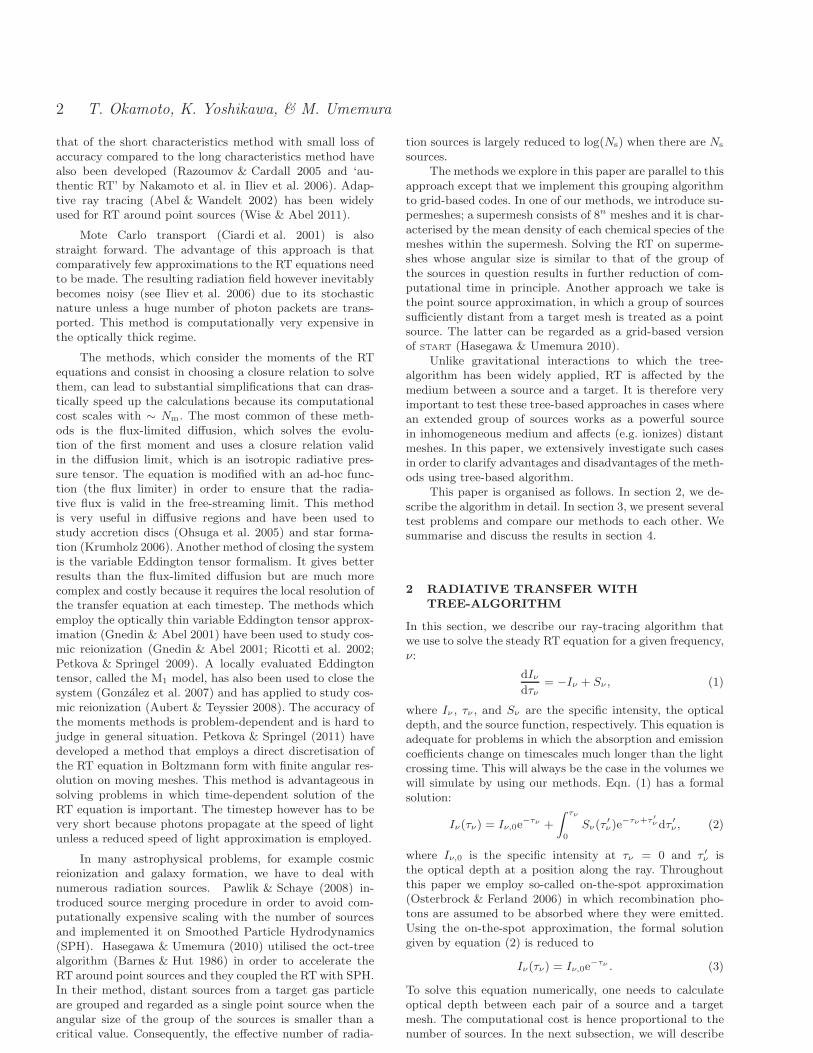
Figure 4. Test 1 – Images of the H i fraction, cut through at themid plane of the simulation box at t = 500 Myr.

the most widely used test. Note however that since thereis only a single radiation source, our RT schemes describedin Sections 2.2 and 2.3 have no difference and both meth-ods become the long characteristics method. The aim of thistest is hence to test our chemical reaction solver and timestepping procedure.

We adopt a monochromatic radiation source thatsteadily emits Nγ photons per second, whose frequency isthe Lyman limit frequency (hνL = 13.6 eV). The densityof the initially neutral gas is nH. Assuming the ionizationequilibrium, the Stromgren radius is given by

rS =

(

3Nγ

4παB(T )n2H

)1/3

, (29)

where αB is the Case B recombination coefficient. If we as-sume that the ionization front (I-front) is infinitely thin, theevolution of the I-front radius is analytically given by

rI = rS [1− exp(−t/trec)]1/3 , (30)

where

trec = (nHαB)−1 (31)

is the recombination time.The analytical solution for the profile of the neu-

tral and ionized fractions (XHI(r) = nHI(r)/nH andXHII(r) = nHII(r)/nH) can also be calculated (e.g.Osterbrock & Ferland 2006) from the equation of the ion-ization balance at radius r:

nHI(r)

4πr2Nγe

−τ(r)σHI(νL) = nHII(r)2αB(T ), (32)

where

τ (r) = σHI

∫ r

0

nHI(r′)dr′. (33)

The profile of the neutral fraction is thus given by

XHI(r) =2 +

Nγe−τ(r)σHI

4πr2nHαB−

√

(

2 +Nγe−τ(r)σHI

4πr2nHαB

)2

− 4

2.

(34)

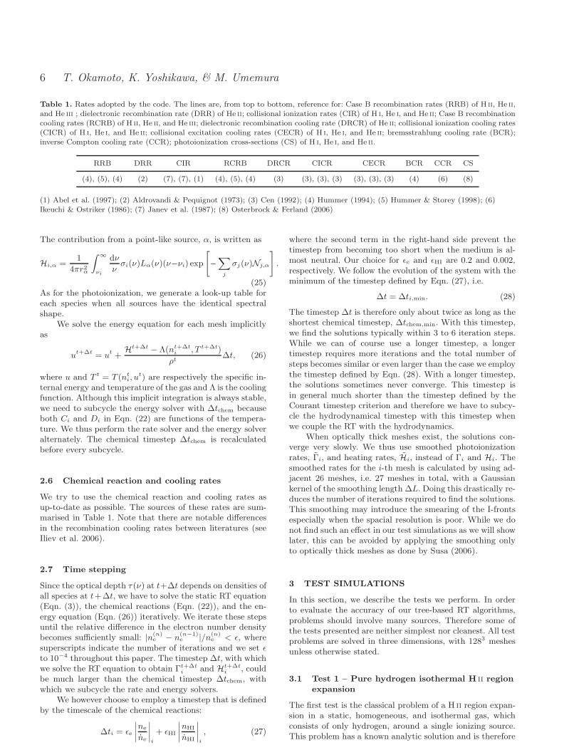
Figure 5. Test 1 – The profiles of ionized and neutral fractions.The radius is in units of the Stromgren radius. The dot-dot-dot-dashed, dotted, dot-dashed, and dashed lines represent simulatedresults at t = 120, 250, 500, and 1000 Myr, respectively. The solidline indicates the analytical solution at t = ∞ given by Eqn. (34).The minimum ionized fraction in the numerical results is set bythe collisional ionization which is not included in the analyticalsolution.

To derive this profile, we ignore the collisional ionization,which is included in our simulations.

The initial physical parameters of this test are thesame as those of Test 1 in Cosmological Radiative TransferComparison Project (Iliev et al. 2006), where the hydrogennumber density, nH, is 10−3 cm−3, the temperature of theisothermal gas is 104 K, and ionization rate, Nγ , is 5× 1048

photons s−1. Given these parameters and the recombinationrate we use, αB(10

4 K) = 2.58×10−13 cm3 s−1, the recombi-nation time and the Stroemgren radius are trec = 122.6 Myrand rS = 5.4 kpc, respectively.

We employ identical numerical parameters to those inIliev et al. (2006): The side length of the simulation box is6.6 kpc, initial ionization fraction is set to 1.2× 10−3 , and aradiation source is placed at the corner of the box, (0, 0, 0).We compare our simulation results to the analytical solutiongiven by Eqn. (34) which represents the solution at t = ∞.

In Fig. 4, we show the neutral fraction in the z = 0.5∆Lplane at t = 500 Myr, at which point the I-front is close toto the maximum radius, i.e. the Stromgren radius. The H ii

region is nicely spherical, though this is not surprising be-cause, with a single source, our method is identical to thelong characteristics method. In Fig. 5, we show the profiles ofionized and neutral fractions at t = 120, 250, 500, and 1000Myr. The results asymptotically approach to the analyticalsolution at t = ∞. There is a minimum neutral fraction inthe simulation results, which is set by the collisional ioniza-tion that is not included in the analytical solution.

c© 2009 RAS, MNRAS 000, 1–13

8 T. Okamoto, K. Yoshikawa, & M. Umemura

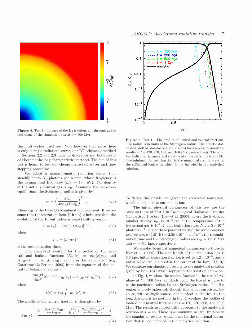
Figure 6. Test 2 – Upper panel: Spherically averaged ionized andneutral fraction profiles. The dot-dashed, dashed, and solid linesindicate indicate the profile at t = 10, 100, and 500 Myr, respec-tively. The results from a high-resolution spherically symmetricone-dimensional simulation are shown by the dotted lines, whichalmost perfectly overlap with those by the three-dimensional sim-ulation. The radius is in units of the Stromgren radius for the uni-form isothermal gas with nH = 10−3 cm−1 and T = 104 K. Lowerpanel: Spherically averaged temperature profiles. The meaning ofthe lines is the same as in the upper panel.

3.2 Test 2 – Pure hydrogen H ii region expansion

with thermal evolution

Test 2 solves essentially the same problem as Test 1, butthe ionizing source is assumed to have a 105 K blackbodyspectrum and we allow the gas temperature to vary owingto heating and cooling processes. The initial gas tempera-ture and ionized fraction are set to 102 K and 1.2 × 10−3,respectively.

In Fig. 6, we show the neutral and ionized fractionprofiles (upper panel) and the temperature profiles (lowerpanel) at t = 10, 100, and 500 Myr. We also show theresults from a high-resolution spherically symmetric one-dimensional simulation by the dotted line. For the one-

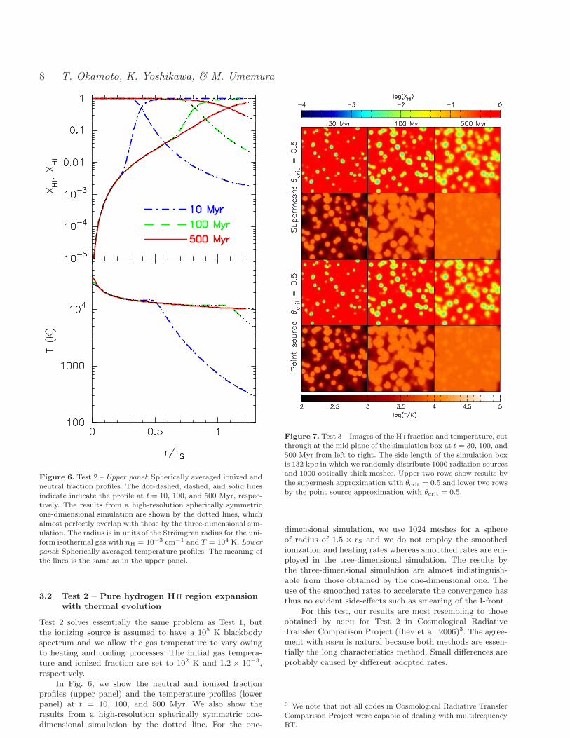
Figure 7. Test 3 – Images of the H i fraction and temperature, cutthrough at the mid plane of the simulation box at t = 30, 100, and500 Myr from left to right. The side length of the simulation boxis 132 kpc in which we randomly distribute 1000 radiation sourcesand 1000 optically thick meshes. Upper two rows show results bythe supermesh approximation with θcrit = 0.5 and lower two rowsby the point source approximation with θcrit = 0.5.

dimensional simulation, we use 1024 meshes for a sphereof radius of 1.5 × rS and we do not employ the smoothedionization and heating rates whereas smoothed rates are em-ployed in the tree-dimensional simulation. The results bythe three-dimensional simulation are almost indistinguish-able from those obtained by the one-dimensional one. Theuse of the smoothed rates to accelerate the convergence hasthus no evident side-effects such as smearing of the I-front.

For this test, our results are most resembling to thoseobtained by RSPH for Test 2 in Cosmological RadiativeTransfer Comparison Project (Iliev et al. 2006)3. The agree-ment with RSPH is natural because both methods are essen-tially the long characteristics method. Small differences areprobably caused by different adopted rates.

3 We note that not all codes in Cosmological Radiative TransferComparison Project were capable of dealing with multifrequencyRT.

c© 2009 RAS, MNRAS 000, 1–13

ARGOT: Accelerated radiative transfer 9

Figure 8. Test 3 – Dependence on the accuracy parameter θcrit.Upper panels: The volume fractions of the neutral fraction att = 500 Myr. The results by the supermesh approximation arepresented in the left panel. The solid (black), dotted (red), anddashed (blue) lines indicate the results with θcrit = 1.0, 0.5, and0.0, respectively. The relative difference to the long characteristicsmethod (θcrit = 0), ∆, is also shown. The right panel shows theresults obtained by the point source approximation. Lower panels:The volume fractions of the gas temperature at t = 500 Myr. Themeaning of the lines are the same as in the upper panels.

3.3 Test 3 – Multiple radiation sources in a

clumpy medium

In order to test the validity of the RT solver based-on thesource grouping, we have to solve problems that involvemultiple sources. Moreover, the error in the supermesh ap-proximation becomes large when the inhomogeneity of themedium is large (see Eqn. (11)). In this test, we thereforesolve the RT from multiple sources in the clumpy medium.The side length of the simulation box is 132 kpc. We ran-domly select 1000 optically thick meshes whose hydrogennumber density is nH = 0.2 cm−3 and optical depth atthe Lyman limit frequency is ∼ 4 × 103 for the mesh size.The hydrogen number density of other meshes is set tonH = 10−3 cm−3. We also randomly distribute 1000 radia-tion sources in the simulation box. Each source has a 105 Kblackbody spectrum and steadily emits Nγ = 5× 1048 ion-izing photons per second. The initial gas temperature andionization fraction are set to 102 K and 1.2 × 10−3, respec-tively.

In Fig. 7, we show the neutral fraction and tempera-

Figure 9. Test 3 – Relative difference in the temperature, cutthrough at the mid plane of the simulation box at t = 500 Myr.This figure compares temperature obtained by the supermesh ap-proximation with θcrit = 1 to that by the long characteristicsmethod (θcrit = 0). The relative difference in temperature is de-

fined as ∆T = (T |supermeshθcrit=1 − T |long)/ T |long.

ture maps at the mid plane of the simulation box at t = 30,100, and 500 Myr. We show the results by the supermeshapproximation and by the point source approximation withθcrit = 0.5. The results by two methods are virtually iden-tical to each other including the shape of shadows by theoptically thick meshes.

In order to investigate the dependence on the accuracyparameter θcrit, we compare the simulations with θcrit = 1,0.5, and 0. In Fig. 8, we show the volume fractions of theneutral fraction and the volume fractions of the gas temper-ature respectively in the upper panels and lower panels. Wealso show difference in the volume fractions relative to thoseobtained by the long characteristics method (θcrit = 0). Forexample, the relative difference in the volume fraction ofthe neutral fraction by the supermesh approximation withθcrit = x is defined as

∆ =p(XH i

)∣

∣

supermesh

θcrit=x− p(XH i

) |long

p(XH i)∣

∣

long

. (35)

The volume fractions of the neutral fraction with θcrit =1 and 0.5 agree quite well with those by the long character-istics method (θcrit = 0). The relative differences are typi-cally less than 1 % even with θcrit = 1. For a given valueof the accuracy parameter, the point source approximationshows slightly better agreement with the long characteris-tics method. On the other hand, agreement in the volumefraction of the gas temperature is not as excellent as that forthe neutral fraction. In particular, both the supermesh andpoint source approximation predict much more low temper-

c© 2009 RAS, MNRAS 000, 1–13

10 T. Okamoto, K. Yoshikawa, & M. Umemura

ature gas around 103 K. This is because treating a sourcegroup as a point source underestimates the surface are ofthe ionized regions as we stated in Section 2.3 and the lowtemperature gas is primarily heated by high energy photonsthat permeate beyond the surfaces of highly ionized regions.Except for this disagreement for the low temperature gas(. 2× 103 K), typical difference is less than 10 %.

To study how serious the deviation from the long char-acteristics method at low temperature, we compare the tem-perature map obtained by the supermesh approximation(θcrit = 1), which shows the worst agreement with the longcharacteristics method, and that by the long characteristicsmethod in Fig. 9. We find that the temperature difference islargest for the low temperature gas with T ∼ 103 K (see alsoFig. 7). The difference in temperature is however very small,only 10 % at most. We therefore conclude that the resultswith θcrit = 1 are almost converged to the result obtainedby the long characteristics method.

This test proves that both tree-based methods produceequally good results even with a large value of the accuracyparameter, θcrit = 1, in the situation where a local H ii regionis driven primarily by one or a few sources. This situation isresembling to the early stage of cosmic reionization. Only atvery late stage of the reionization, the H ii regions overlapeach other and multiple sources become visible each other;at this stage, the reionization has largely completed already.We thus expect that our tree-based methods, in particularthe supermesh approximation, are well suited to this typeof problems.

3.4 Test 4 – Clustered radiation sources in a

clumpy medium

Unlike Test 3, here we explore the problem in which groupsof sources act like bright extended sources and they ionizedistant meshes. This would be one of the toughest problemsfor the methods accelerated by source grouping. The sidelength of the simulation box is the same as in Test 3, i.e.Lbox = 132 kpc. In order to construct clustered distributionof radiation sources, we put a sphere of radius r = Lbox/4,whose centre is randomly placed in the simulation box. Weuniformly distribute 1000 radiation sources in the sphere.We then put a new sphere whose radius is 20% smaller thanthe previous one and again we distribute 1000 sources in thesphere. We continue this procedure until we put 10 spheres,each of which contains 1000 sources. Consequently, thereare 104 radiation sources in the simulation box. Each sourcehas a 105 K blackbody spectrum and emits Nγ = 5 × 1048

ionizing photons per second. We also randomly select 104

optically thick meshes whose hydrogen number density isnH = 0.2 cm−3. The hydrogen number density of the re-maining meshes is set to nH = 10−3 cm−3. The initial gastemperature and ionization fraction are set to 102 K and1.2× 10−3, respectively.

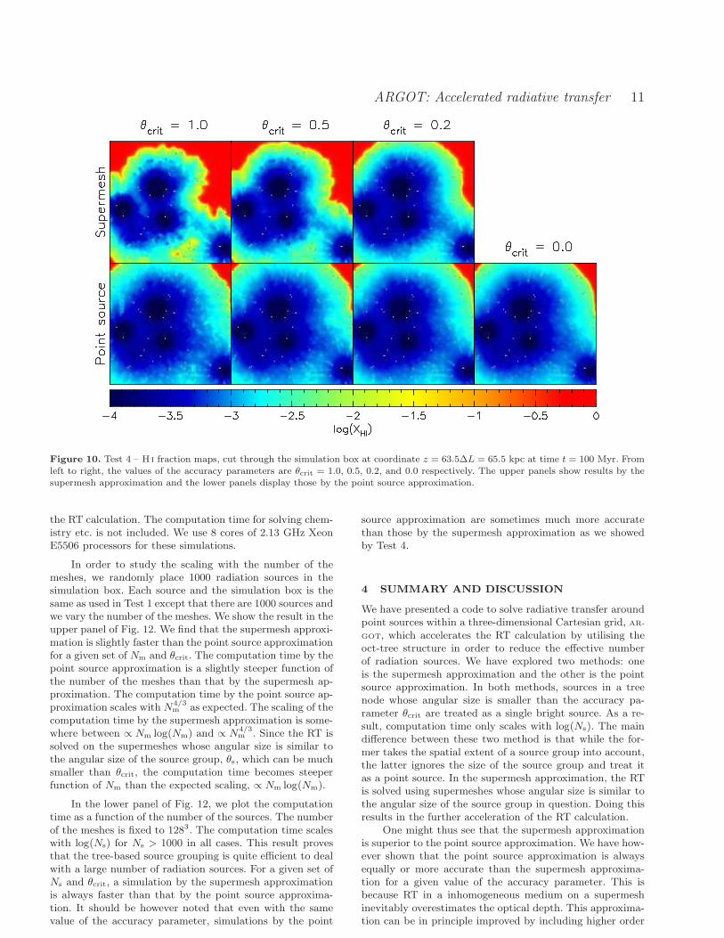
In Fig. 10, we show the neutral fraction maps, cutthrough at the mid plane of the simulation box. The size andshape of the ionized regions by the supermesh approxima-tion strongly depend on the value of the accuracy parameter;The larger the value is, the smaller the size of the ionizedregions is. This is due to the very nature of the supermeshapproximation, which significantly overestimates the opticaldepth when a size of supermesh is large and the variance of

the H i density is large (see Eqn. (11) and (12)). On theother hand, the results by the point source approximationare relatively insensitive to the value of the accuracy param-eter. The size of the ionized regions is almost same betweenθcrit = 1 and 0 while small difference is seen in the shapes.

In Fig. 11, we show the volume fractions of the neu-tral fraction and gas temperature at t = 100 Myr varyingthe value of the accuracy parameter, θcrit, from 1 to 0. Wealso show the relative difference to the long characteristicsmethod (θcrit = 0). The volume fraction of the neutral frac-tion confirms the dependence of the supermesh approxima-tion on the value of the accuracy parameter, i.e. the largerthe value of θcrit is, the smaller the ionized fraction is. Thisdependence is more evident in the volume fraction of thegas temperature. There is more low temperature gas in thesimulation with a larger value of the accuracy parameter.Importantly, the results by the supermesh approximationwith θcrit = 0.2 still significantly deviate from those by thelong characteristics methods, and therefore we cannot trustthe result even with θcrit = 0.2.

On the other hand, the result by the point source ap-proximation with θcrit = 1 shows an excellent agreementwith that with the long characteristics method, in spite ofthe fact that this approximation ignores the spatial extentof source groups. This result proves that the point sourceapproximation is very efficient and accurate for this type ofproblems.

The relative difference to the long characteristicsmethod indicates that both approximations overestimatesthe volume fraction of the almost fully-ionized gas (XH i

≃2 × 10−6). This ionized fraction corresponds to the centralregions of each source spheres. The volume of these regionsare however very small and the neutral fraction is very lowanyway; this overestimation of the ionization fraction at thecentral regions of the source spheres does not affect the evo-lution of the whole simulation box. In fact, by the pointsource approximation, the relative difference to the longcharacteristics method in the volume fraction of the neu-tral fraction is typically 1 % and ∼ 10 % at most except forthe highly ionized gas with XH i

. 10−5.Even by the point source approximation, the relative

difference in the volume fraction of the gas temperature tothe long characteristics method is rather large for the lowtemperature gas. The gas temperature however agrees verywell with that by the long characteristics method just as weshowed for Test 3. Except for the low temperature gas, thetypical difference is ∼ 10 %. Interestingly, decreasing thevalue of the accuracy parameter in the point source approx-imation from 1 to 0.2 does not improve the agreement withthe long characteristics method very much in spite of thefact that the simulations with a smaller value of the accu-racy parameter is much more computationally expensive aswe will show in the next subsection. Since the point sourceapproximation with θcrit = 1 seems to be sufficiently ac-curate, we expect that this approximation with θcrit = 0.5would be a safe choice for most types of problems.

3.5 Code performance

We here investigate how the computation time scales withthe number of meshes and that of the sources. For this pur-pose, we measure the wall-clock time taken for one step of

c© 2009 RAS, MNRAS 000, 1–13

ARGOT: Accelerated radiative transfer 11

Figure 10. Test 4 – H i fraction maps, cut through the simulation box at coordinate z = 63.5∆L = 65.5 kpc at time t = 100 Myr. Fromleft to right, the values of the accuracy parameters are θcrit = 1.0, 0.5, 0.2, and 0.0 respectively. The upper panels show results by thesupermesh approximation and the lower panels display those by the point source approximation.

the RT calculation. The computation time for solving chem-istry etc. is not included. We use 8 cores of 2.13 GHz XeonE5506 processors for these simulations.

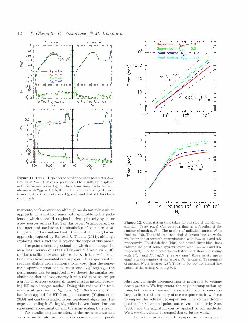
In order to study the scaling with the number of themeshes, we randomly place 1000 radiation sources in thesimulation box. Each source and the simulation box is thesame as used in Test 1 except that there are 1000 sources andwe vary the number of the meshes. We show the result in theupper panel of Fig. 12. We find that the supermesh approxi-mation is slightly faster than the point source approximationfor a given set of Nm and θcrit. The computation time by thepoint source approximation is a slightly steeper function ofthe number of the meshes than that by the supermesh ap-proximation. The computation time by the point source ap-proximation scales with N

4/3m as expected. The scaling of the

computation time by the supermesh approximation is some-where between ∝ Nm log(Nm) and ∝ N

4/3m . Since the RT is

solved on the supermeshes whose angular size is similar tothe angular size of the source group, θs, which can be muchsmaller than θcrit, the computation time becomes steeperfunction of Nm than the expected scaling, ∝ Nm log(Nm).

In the lower panel of Fig. 12, we plot the computationtime as a function of the number of the sources. The numberof the meshes is fixed to 1283. The computation time scaleswith log(Ns) for Ns > 1000 in all cases. This result provesthat the tree-based source grouping is quite efficient to dealwith a large number of radiation sources. For a given set ofNs and θcrit, a simulation by the supermesh approximationis always faster than that by the point source approxima-tion. It should be however noted that even with the samevalue of the accuracy parameter, simulations by the point

source approximation are sometimes much more accuratethan those by the supermesh approximation as we showedby Test 4.

4 SUMMARY AND DISCUSSION

We have presented a code to solve radiative transfer aroundpoint sources within a three-dimensional Cartesian grid, AR-

GOT, which accelerates the RT calculation by utilising theoct-tree structure in order to reduce the effective numberof radiation sources. We have explored two methods: oneis the supermesh approximation and the other is the pointsource approximation. In both methods, sources in a treenode whose angular size is smaller than the accuracy pa-rameter θcrit are treated as a single bright source. As a re-sult, computation time only scales with log(Ns). The maindifference between these two method is that while the for-mer takes the spatial extent of a source group into account,the latter ignores the size of the source group and treat itas a point source. In the supermesh approximation, the RTis solved using supermeshes whose angular size is similar tothe angular size of the source group in question. Doing thisresults in the further acceleration of the RT calculation.

One might thus see that the supermesh approximationis superior to the point source approximation. We have how-ever shown that the point source approximation is alwaysequally or more accurate than the supermesh approxima-tion for a given value of the accuracy parameter. This isbecause RT in a inhomogeneous medium on a supermeshinevitably overestimates the optical depth. This approxima-tion can be in principle improved by including higher order

c© 2009 RAS, MNRAS 000, 1–13

12 T. Okamoto, K. Yoshikawa, & M. Umemura

Figure 11. Test 4 – Dependence on the accuracy parameter θcrit.Results at t = 100 Myr are presented. The results are displayedin the same manner as Fig. 8. The volume fractions for the sim-ulation with θcrit = 1, 0.5, 0.2, and 0 are indicated by the solid(black), dotted (red), dot-dashed (green), and dashed (blue) lines,respectively.

moments, such as variance, although we do not take such anapproach. This method hence only applicable to the prob-lems in which a local H ii region is driven primarily by one ora few sources such as Test 3 in this paper. When one appliesthe supermesh method to the simulation of cosmic reioniza-tion, it could be combined with the ‘local clumping factor’approach proposed by Raicevic & Theuns (2011), althoughexploring such a method is beyond the scope of this paper.

The point source approximation, which can be regardedas a mesh version of START (Hasegawa & Umemura 2010),produces sufficiently accurate results with θcrit = 1 for alltest simulations presented in this paper. This approximationrequires slightly more computational cost than the super-mesh approximation and it scales with N

4/3m log(Ns). The

performance can be improved if we choose the angular res-olution so that at least one ray from a radiation source (ora group of sources) crosses all target meshes instead of solv-ing RT to all target meshes. Doing this reduces the totalnumber of rays from ∝ Nm to ∝ N

2/3m . Such an algorithm

has been applied for RT from point sources (Yajima et al.2009) and can be extended to our tree-based algorithm. Theexpected scaling is Nm logNs, which is even faster than thesupermesh approximation and the same scaling by START.

For parallel implementation, if the entire meshes andsources can fit into memory of one computer node, paral-

Figure 12. Computation time taken for one step of the RT cal-culation. Upper panel: Computation time as a function of thenumber of meshes, Nm. The number of radiation sources, Ns isfixed to 1000. The solid (red) and dashed (green) lines show theresults by the supermesh approximation with θcrit = 1 and 0.5,respectively. The dot-dashed (blue) and dotted (light blue) linesindicate the point source approximation with θcrit = 1 and 0.5,respectively. The thin dot-dot-dot-dashed lines show the scaling

with N4/3m and Nm log(Nm). Lower panel: Same as the upper

panel but the number of the source, Ns, is varied. The numberof meshes, Nm is fixed to 1283. The thin dot-dot-dot-dashed lineindicates the scaling with log(Ns).

lelisation via angle decomposition is preferable to volumedecomposition. We implement the angle decomposition byusing both MPI and OpenMP. If a simulation size becomes toolarge to fit into the memory of one computer node, we haveto employ the volume decomposition. The volume decom-position for RT around point sources was introduce by Susa(2006) and the algorithm can be applied to our methods.We leave the volume decomposition to future work.

The method presented in this paper can be easily com-

c© 2009 RAS, MNRAS 000, 1–13

ARGOT: Accelerated radiative transfer 13

bined with any grid-based hydrodynamic code, even withcodes based on AMR (Fryxell et al. 2000; Teyssier 2002;O’Shea et al. 2004) and will be useful for various astrophysi-cal problems in which a large number of radiation sources arerequired such as cosmic reionization and galaxy formation.We will apply our code for these issues in a forth comingpaper.

ACKNOWLEDGEMENTS

We would like to thank Kenji Hasegawa and Hideki Ya-jima for stimulating discussion. We are also grateful to theanonymous referee for helpful comments. The simulationswere performed with FIRST and T2K Tsukuba at Centre forComputational Sciences in University of Tsukub and withthe Cray XT4 at CfCA of NAOJ. This work was supportedin part by the FIRST project based on Grants-in-Aid forSpecially Promoted Research by MEXT (16002003), Grant-in-Aid for Scientific Research (S) by JSPS (20224002). TOacknowledges financial support by Grant-in-Aid for YoungScientists (start-up: 21840015).

REFERENCES

Abel T., Anninos P., Zhang Y., Norman M. L., 1997,New Astron., 2, 181

Abel T., Norman M. L., Madau P., 1999, ApJ, 523, 66Abel T., Wandelt B. D., 2002, MNRAS, 330, L53Aldrovandi S. M. V., Pequignot D., 1973, A&A, 25, 137Anninos P., Zhang Y., Abel T., Norman M. L., 1997,New Astron., 2, 209

Aubert D., Teyssier R., 2008, MNRAS, 387, 295Barnes J., Hut P., 1986, Nat, 324, 446Cen R., 1992, ApJS, 78, 341Ciardi B., Ferrara A., Marri S., Raimondo G., 2001, MN-RAS, 324, 381

Fryxell B., et al., 2000, ApJS, 131, 273Gnedin N. Y., Abel T., 2001, New Astron., 6, 437Gonzalez M., Audit E., Huynh P., 2007, A&A, 464, 429Hasegawa K., Umemura M., 2010, MNRAS, 407, 2632Hummer D. G., 1994, MNRAS, 268, 109Hummer D. G., Storey P. J., 1998, MNRAS, 297, 1073Ikeuchi S., Ostriker J. P., 1986, ApJ, 301, 522Iliev I. T., et al., 2006, MNRAS, 371, 1057—, 2009, MNRAS, 400, 1283Janev R. K., Langer W. D., Evans K., 1987, Elementaryprocesses in Hydrogen-Helium plasmas - Cross sectionsand reaction rate coefficients, Janev, R. K., Langer, W. D.,& Evans, K., ed. Springer

Krumholz M. R., 2006, ApJL, 641, L45Kunasz P., Auer L. H., 1988, J. Quant. Spectrosc. Ra-diat. Transfer, 39, 67

Mellema G., Raga A. C., Canto J., Lundqvist P., BalickB., Steffen W., Noriega-Crespo A., 1998, A&A, 331, 335

Nakamoto T., Umemura M., Susa H., 2001, MNRAS, 321,593

Ohsuga K., Mori M., Nakamoto T., Mineshige S., 2005,ApJ, 628, 368

O’Shea B. W., Bryan G., Bordner J., Norman M. L., Abel

T., Harkness R., Kritsuk A., 2004, ArXiv Astrophysicse-prints:astro-ph/0403044

Osterbrock D. E., Ferland G. J., 2006, Astrophysics ofgaseous nebulae and active galactic nuclei, 2nd edn., Os-terbrock, D. E. & Ferland, G. J., ed. University ScienceBooks

Pawlik A. H., Schaye J., 2008, MNRAS, 389, 651Petkova M., Springel V., 2009, MNRAS, 396, 1383—, 2011, MNRAS, 415, 3731Raicevic M., Theuns T., 2011, MNRAS, 412, L16Razoumov A. O., Cardall C. Y., 2005, MNRAS, 362, 1413Ricotti M., Gnedin N. Y., Shull J. M., 2002, ApJ, 575, 33Sokasian A., Abel T., Hernquist L. E., 2001, New Astron.,6, 359

Stone J. M., Mihalas D., Norman M. L., 1992, ApJS, 80,819

Susa H., 2006, PASJ, 58, 445Teyssier R., 2002, A&A, 385, 337Wise J. H., Abel T., 2011, MNRAS, 414, 3458Yajima H., Umemura M., Mori M., Nakamoto T., 2009,MNRAS, 398, 715

Yoshikawa K., Sasaki S., 2006, PASJ, 58, 641

This paper has been typeset from a TEX/ LATEX file preparedby the author.

c© 2009 RAS, MNRAS 000, 1–13