A review of the Henon map and its physical interpretations

Haoran Wen∗School of Physics

Georgia Institute of Technology,Atlanta, GA 30332-0430, U.S.A

(Dated: April 21, 2014)

The Henon map is one of the simplest two-dimensional mappings exhibiting chaotic behavior.It has been extensively studied due to its low dimension and chaotic dynamics. Even though theHenon map is introduced mathematically as a model problem and has no particular physical importof itself, links between certain harmonic oscillators and “Henon-like” maps have been found. Toget a better understanding of the Henon map, we review the dynamic properties of the Henon mapincluding its fixed points, stability, periodic orbits, and so on, and a physical interpretation of it isdiscussed.

Georgia Tech PHYS 7224:NONLINEAR DYNAMICScourse project, spring semester 2014

I. INTRODUCTION

In 1963, Lorenz proposed a system of three coupleddifferential equations, which is later well known as theLorenz flow. The Lorenz flow was first studied becauseit is of interest for weather prediction. However, furtherexplorations of the Lorenz flow have revealed even morebenefits. As an illustration of deterministic chaos, theLorenz flow was widely explored and studied. Motivatedby the Lorenz equations, Henon introduced a simple twodimensional map in 1976 [1], which captured the stretch-ing and folding dynamics of chaotic systems such as theLorenz system.The Henon map is a minimal normal form for mod-

eling flows near a saddle-node bifurcation, and it is aprototype of the stretching and folding dynamics thatleads to deterministic chaos. Due to its simple form, theHenon map has provide us a way to conduct more de-tailed exploration of the chaotic dynamics. Interestingenough, even though the Henon map is introduced as amathematical model, it still corresponds to the dynam-ics of some physical systems, one of which was given byBiham and Wenzel [2]. However, this interpretation ismostly exploited as a computational tool instead of anillustration of the physical dynamics. In contrast, Heagydemonstrated an interesting interpretation of the Henonmap [3]. This interpretation links the Henon map to theperiod one return map of an impulsively driven harmon-ic oscillator, which provides a relatively good insight intothe dynamics of the Henon map.In sect. II the standard form of the Henon map is in-

troduced and the details of its dynamic properties arediscussed. A review of an physical interpretation of theHenon map is shown in sect. III. In sect. IV the prop-

∗Electronic address: hwen37@mail.gatech.edu

erties of the Henon map are briefly summarized, and adiscussion of its physical interpretations is given.

II. THE HENON MAP

In 1969, Henon showed in Ref [4] that essential prop-erties of dynamical systems defined by differential e-quations can be retained by a carefully defined area-preserving mappings. Inspired by the same idea, Henonproposed the famous two dimensional Henon map as areduced approach to study the dynamics of the Lorenzsystem. The Henon map is given by the following equa-tions:

xn+1 = 1− ax2n + byn

yn+1 = xn

(1)

This is a nonlinear two dimensional map, which can alsobe written as a two-step recurrence relation

xn+1 = 1− ax2n + bxn−1 (2)

A. Fixed points and Henon attractor

An attractor refers to a subset of a connected statespace M0, where the flow is globally contracting onto,as M0 mapping into itself under forward evolutions. Anattractor can be a fixed point, a periodic orbit, aperiodic,or a combination of the above. The most interesting caseis the aperiodic recurrent attractor, which is also referredto as a strange attractor.

For the Henon map, we have two fixed points. Taking(xn+1, yn+1) = (xn, yn) = (x0, x0) in (1), we have

x0 =−(1− b)±√

(1− b)2 + 4a

2a(3)

which can be either attracting or saddle points dependingon the choice of parameters (a, b) [5].

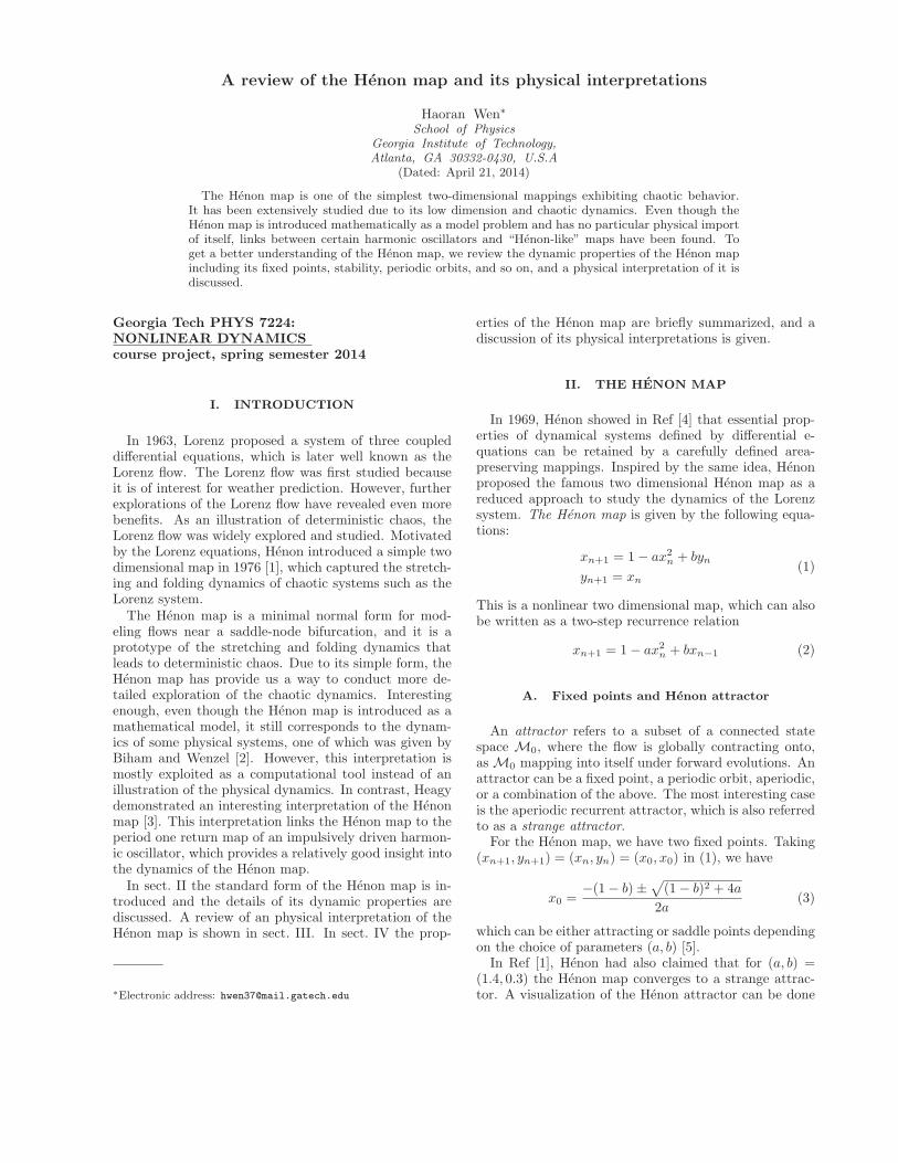
In Ref [1], Henon had also claimed that for (a, b) =(1.4, 0.3) the Henon map converges to a strange attrac-tor. A visualization of the Henon attractor can be done

2

−1.5 −1 −0.5 0 0.5 1 1.5−1.5

−1

−0.5

0

0.5

1

1.5

xn

x n+1

FIG. 1: A visualization of the Henon attractor.

by numerical iterations. By picking an arbitrary initialpoint and iterating (1) on a computer and plotting theresults on the (xn, xn+1) plane, we can get a sketch ofthe dynamics of the Henon map. An iteration of 10, 000with initial point (0.1, 0.1) is plotted in Fig. 1. As wehave mentioned, the Henon map is one of the simplestmaps capturing the stretching and folding dynamics ofchaotic systems. The parameter a controls the amountof stretching and the parameter b controls the thicknessof folding. In Fig. 1, b is relatively large and the attrac-tor is rather thick, which gives a clearly visible transversefractal structure.It is worth mentioning that even though the Henon

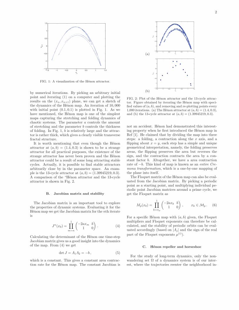
attractor at (a, b) = (1.4, 0.3) is shown to be a strangeattractor for all practical purposes, the existence of thestrange attractor has never been proven and the Henonattractor could be a result of some long attracting stablecycles. Actually, it is possible to find stable attractorsarbitrarily close by in the parameter space. An exam-ple is the 13-cycle attractor at (a, b) = (1.39945219, 0.3).A comparison of the “Henon attractor and the 13-cycleattractor is shown in Fig. 2.

B. Jacobian matrix and stability

The Jacobian matrix is an important tool to explorethe properties of dynamic systems. Evaluating it for theHenon map we get the Jacobian matrix for the nth iterateis

Jn(x0) =1∏

m=n

(−2axm b1 0

). (4)

Calculating the determinant of the Henon one time-stepJacobian matrix gives us a good insight into the dynamicsof the map. From (4) we get

det J = Λ1Λ2 = −b , (5)

which is a constant. This gives a constant area contrac-tion rate for the Henon map. The constant Jacobian is

(a)−1.5 −1 −0.5 0 0.5 1 1.5

−1.5

−1

−0.5

0

0.5

1

1.5

xn

x n+1

(b)−1.5 −1 −0.5 0 0.5 1 1.5

−1.5

−1

−0.5

0

0.5

1

1.5

xn

x n+1

FIG. 2: Plot of the Henon attractor and the 13-cycle attrac-tor. Figure obtained by iterating the Henon map with speci-fied values of (a, b), and removing and re-plotting points every1,000 iterations. (a) The Henon attractor at (a, b) = (1.4, 0.3),and (b) the 13-cycle attractor at (a, b) = (1.39945219, 0.3).

not an accident. Henon had demonstrated this interest-ing property when he first introduced the Henon map inRef [1]. He claimed that by dividing the map into threesteps: a folding, a contraction along the x axis, and aflipping about x = y, each step has a simple and uniquegeometrical interpretation, namely, the folding preservesareas, the flipping preserves the area but reverses thesign, and the contraction contracts the area by a con-stant factor b. Altogether, we have a area contractionrate of −b. This kind of map is known as an entire Cre-mona transformation, which is a one-by-one mapping ofthe plane into itself.

The Floquet matrix of the Henon map can also be eval-uated from the Jacobian matrix. By picking a periodicpoint as a starting point, and multiplying individual pe-riodic point Jacobian matrices around a prime cycle, weget the Floquet matrix as

Mp(x0) =

1∏k=np

(−2axk b1 0

), xk ∈ Mp . (6)

For a specific Henon map with (a, b) given, the Floquetmultipliers and Floquet exponents can therefore be cal-culated, and the stability of periodic orbits can be eval-uated accordingly (based on |Λj | and the sign of the real

part of the Floquet exponents μ(i)).

C. Henon repeller and horseshoe

For the study of long-term dynamics, only the non-wandering set Ω of a dynamics system is of our inter-est, where the trajectories reenter the neighborhood in-

3

finitely often. A non-wandering set is the union of al-l kinds of separately invariant sets including attractorsand repellers. In sect. II A we have already introducedthe attractor, which is a subset of a connected state s-pace attracting the flow globally. Conversely, for a non-wandering set Ω enclosed by a connected state space vol-ume M0, if all points within M0 but not Ω will eventual-ly exit M0, the non-wandering set Ω is called a repeller.For the Henon map with parameter b �= 0, interesting

repellers can be found. The Henon map takes a rectan-gular area and returns it bent as a Smale horseshoe. TheHenon repeller with parameter b = −1 and a large pa-rameter a is especially instructive. According to (5), forb = −1, the contraction rate is 1, which means the mapis area preserving. At the same time, the map is strong-ly stretching due to a large parameter a. Therefore, weget a strongly stretching but yet area preserving map,where the folded horseshoe can be clearly observed andthe stable manifold Ws and unstable manifold Wu of thecan be studied visually. For parameter (a, b) = (6,−1),different iterates of the map are calculated numericallyand plotted on the (x, y) plane in Fig. 3.Starting with a set of points in a small square around

the fix point x0, iterating forward using (1) will stretchand fold the initial set of points and trace out the un-stable manifold Wu, as indicated by the blue line inFig. 3(a). On the other hand, the backward iterationin time is given by

xn−1 = yn

yn+1 = −b−1(1− ay2n − bxn)(7)

Iterated backward in time, the initial set will outlinethe stable manifold Ws, as indicated by the green linein Fig. 3(a). The intersection of Ws and Wu gives aninvariant and optimal initial region M where the non-wandering set is enclosed. We say M is invariant andoptimal because any point outside Ws border escapes toinfinity forward in time and any point outside Wu bordercomes from infinity backward in time.As we iterate one more step forward in time, M will

be stretched and folded to form a Smale horseshoe, andthe intersection is split into two future strips as shownin Fig. 3(b). Label the strips symbolically we have M0.

and M1. respectively. Similarly, iterate one more stepbackward in time, the intersection becomes four region-s as shown in Fig. 3(c), which can be labeled as M0.0,M0.1, M1.0 and M1.1. Iterate one more step forward,we will get 4 future strips labeled by M00., M01., M10.,M11., and iterate one more step backward, we will get4 past strips labeled by M.00, M.01, M.10, M.11 (Fig-ure 6 in appendix A). As we iterate further, the morefuture strips and past strips will intersect each otherto form more regions which can be labeled as MS−.S+

where S+ = s1s2 · · · sm is called the future itinerary andS− = s−n · · · s−1s0 is called the past itinerary. As onemay notice, the dynamics of the map is simply acting asa shift of the itinerary, where a forward iterate move theentire itinerary to the left through the ‘decimal point’ and

(a)−1 −0.5 0 0.5 1−1

−0.8

−0.6

−0.4

−0.2

0

0.2

0.4

0.6

0.8

1

x

y

(b)−1 −0.5 0 0.5 1−1

−0.8

−0.6

−0.4

−0.2

0

0.2

0.4

0.6

0.8

1

x

y

(c)−1 −0.5 0 0.5 1−1

−0.8

−0.6

−0.4

−0.2

0

0.2

0.4

0.6

0.8

1

x

y

FIG. 3: Different iterates of the Henon map at (a, b) =(6,−1). The two fixed points are marked as red circles. Theblue line corresponds to forward iterates, and the green linecorresponds to backward iterates. (a) Forward iterate show-ing Wu, and backward iterate showing Ws. The intersectionbounds the state space M, containing the non-wandering setΩ. (b) One more forward iterate. The intersection of f(M)and M becomes two strips. (c) One more backward iterate.The intersection of f(M) and f−1(M) becomes four regions.

a backward iterate move the entire itinerary to the right.Therefore, we call the set of all bi-infinite itineraries thatcan be define by S = S−.S+ the full shift.

Here we say the Henon map shows a complete Smalehorseshoe because it has a complete binary symbolicdynamics, and as we can see in Fig. 3, every forwardfold fn(M) intersects transversally every backward foldf?m(M). For a given step number m and n, the inter-sections MS−.S+ represents the set of points that do notescape in such forward and backward iterates. Therefore,when m and n goes to infinity, we get the set of pointsthat remain inM for all time, namely, the non-wanderingset of M.

Ω =

{x : x ∈ lim

m,n→∞ fm(M.)⋂

f−n(M.)

}. (8)

However, the non-wandering set for an arbitrary mapdoesn’t necessarily corresponds to the full shift, becausesome points represented by the itinerary in the full shiftmay be inadmissible. Thus we say the complete dynam-ics of the Henon map is a subshift where all admissible

4

sequences are considered.The reason why we carry it all the way through to

show the Henon map corresponds to a complete Smalehorse is that, a complete Smale horseshoe is structural-ly stable, meaning that all intersections of forward andbackward iterates of M remain transverse for sufficient-ly small variations of the Henon map parameters a andb. In a more physical term, the transport properties ofthe system have a smooth dependence on the parameter-s. Structural stability is an extremely desirable howeverrather rare property. A lack of structural stability willresults in the creation and destruction of infinitely manyperiodic orbits for any parameter change, no matter howsmall it is. For any structurally unstable systems, evenas simple as a purely hyperbolic system, any global ob-servable could show a non-smooth dependence on systemparameters and behave in a rather unpredictable way.Therefore, the fact that for a specific range of parameters[6] the Henon map is structural stable is a very importantproperty and what makes any physical interpretation ofthe Henon map practically meaningful.

D. Symmetries and Hamiltonian flow

The symmetry of the Henon is rather simple. For aparameter b �= 0, the Henon is time reversible with theback ward iteration given by (7), thus giving a b to 1/b,a to a/b2 symmetry in the parameter plane, and an x to−x/b symmetry in the coordinate plane.Some interesting properties for the Henon map with

parameter b = −1 can be found. When b = −1, theHenon map (2) becomes

ax2n = 1− xn+1 − xn−1 . (9)

The map has an x to x symmetry, the backward andthe forward iteration are the same, and according to (5),the area contraction rate is 1. So the map is orientationand area preserving, and the non-wandering set is sym-metric about xn+1 = xn. Such a simple map correspondsto a Poincare return map for a 2-dimensional Hamiltoni-an flow. As we know, for a Hamiltonian flow, the Jaco-bian matrix J is a symplectic transformation, detJ = 1for all the time and the flow is a canonical transforma-tion. This analogue gives us a hint about how we candevelop physical interpretations of the Henon map. Insect. III, we will therefore start with this orientation andarea preserving case and discuss a physical interpretationof the Henon map in detail.

III. PHYSICAL INTERPRETATIONS OF THEHENON MAP

As discussed in sect. IID, the area preserving Henonmap is a good starting point to get insightful physical

views of the Henon map. Actually, different interpreta-tions have been proposed based on the connection be-tween the area-preserving Henon map and the returnmap of the Hamiltonian flow[2, 3, 7]. In this section,we also start our discussion with the area preservingcase, and we choose to review in detail the interpretationdemonstrated by Heagy in ref. [3], because in Heagys pa-per a very comprehensive formulation is developed andmore physical meaning has been given to the interpreta-tion instead of just using it as a computational tool toassist mathematical calculations.

A. Area-preserving case

Kicked oscillator systems have been studied as physi-cal model of different maps. For example, a periodicallykicked pendulum has been shown to have a return mapequivalent to the standard map[8]. In ref. [3], Heagyclaimed that the area preserving Henon map can also beassociated with a kicked driven harmonic oscillator witha cubic nonlinear coupling to the kicking term. This asso-ciation can be derived from the Hamiltonian of the kickedoscillator given by

H =1

2p2 +

1

2x2 +

1

2x3

∞∑n=−∞

δ(t− nT ) . (10)

The Hamilton’s equations for the Hamiltonian(10) are

dx

d t= p ,

d p

d t= −x− x2

∞∑n=−∞

δ(t− nT ) .(11)

Consider one period of the oscillation T , for a smalltime interval (nT, nT + ε) during which the kick takesplace, from the Hamiltons equations(11) we have

dxn = x(nT + ε)− x(nT ) = εp(nT ) ,

d pn = p(nT + ε)− p(nT ) = −εx(nT )− x(nT )2 .(12)

where the prime denote the variables after the kick. Tak-ing the limit of ε → 0 we have

x(nT + ε) = x(nT ) ,

p(nT + ε) = p(nT )− x(nT )2 .(13)

After the kick, for time nT +ε → (n+1)T , the systemgoes freely and integrate (10) we get

x(t) = C1 cos(t− nT ) + C2 sin(t− nT ) ,

p(t) = −C1 sin(t− nT ) + C2 cos(t− nT ) .(14)

Substituting (13) into (14) we get C1 = x(nT ) andC2 = p(nT ) − x(nT )2. Substituting C1, C2 and using a

5

discrete representation given by xn = x(nT ), pn = p(nT ),equations refeqe:nkick become

xn+1 = xn cos(t− nT ) + (pn − x2n) sin(t− nT ) ,

pn+1 = −xn sin(t− nT ) + (pn − x2n) cos(t− nT ) .

(15)

This map is already the same as the area-preservingmap given by Henon in ref. [4]. However, if we want toget the standard form of the Henon map given by (1) or(2), a few more steps need to be taken. First, we write(15) in the two-step recurrent form

xn+1 + xn−1 = 2xn cosT − x2n sinT . (16)

Then we take the linear transformation x = σX +cotT , where σ = (cos2 T − 2 cosT )/ sinT , and set a =cos2 T − 2 cosT . Equation (16) becomes

Xn+1 +Xn−1 = 1− aX2n . (17)

This is identical to the area-preserving case (b = −1) ofequation (2). So we see that the Henon map (1) withb = −1 is actually equivalent to the harmonic oscillatorsystem.

B. Dissipative case

Good and straightforward as the derivation for thearea-preserving case is, it is also quite limited. Ex-am the derivation carefully we find the parameter a =cos2 T − 2 cosT of the Henon map is limited to the inter-val (−1, 3). Therefore, many special chaotic propertiesof the Henon map is not accessible, including the wholesequence of period doubling bifurcations that occurs fora ≥ 3. To better develop the physical interpretation ofthe complete Henon map, the dissipative case is also in-troduced.

Adding a damping term into the oscillator system witha constant damping factor γ, we get the dissipative os-cillator system governed by

dx

d t= p ,

d p

d t= −x− γp− x2

∞∑n=−∞

δ(t− nT ) .(18)

Similar to the area-preserving case, the effect of thekick in each period is also given by (13). However, theevolution between two kicks is a function of γ. For thetime interval (nT + ε, (n+ 1)T ), the system becomes

dx

d t= p ,

d p

d t= −x− γp .

(19)

Solving (19) we have

xn+1 =e−γT/2(xn cos(ωT )

+1

ω(pn − x2

n +1

2γxn) sin(ωT )) ,

pn+1 =e−γT/2[−ωxn sin(ωT )

+ (pn − x2n +

1

2γxn) cos(ωT )− 1

2γxn+1 .

(20)

where ω =√1− 1

4γ2. Again, take a transformation of

coordinate

x =σdX + ω cotωT ,

p =ωσd

sinωTeγT/2

[1 +ω cotωT

σd(1− γ

2ωe−γT/2 sinωT )

+ e−γT/2(cosωT − γ

2ωsinωT )X + Y ]

(21)

where

σd = ω cotωT [e−γT/2 cosωT − (1 + e−γT )] . (22)

This transformation leads us back to the Henon mapgiven by (1), with the parameters given by

a = cosωT [e−γT cosωT − e−γT/2(1 + e−γT )] ,

b = −e−γT .(23)

Expressing a in terms of b we have

a = − cotωT [b cosωT +√−b(1− b)] . (24)

Therefore, by consider the area-contracting case(b <1), parameter a is no more limited to the interval (−1, 3).Yet, this doesn’t make all the dynamic properties acces-sible to the oscillator system. As we have mentioned insect. II A, for a range of parameters (a, b), the Henon maphave two fixed points. One of the fixed point is always un-stable and the other one is at the origin and can be eitherstable or unstable depending on the choice of parameters.More specifically, the origin is stable for a < 3

4 (1 − b)2.For the dissipative harmonic oscillator case, from (24) weknow a ≤ −b +

√−b(1 − b) ≤ 34 (1 − b)2, so the origin is

always stable. However, it is the case where the originis unstable that shows more interesting properties likeperiod doubling and strange attractor[3].

This stability can be broken by modifying the kickcoupling function. Setting the coupling function to bef(x) = Ax+ 1

3x3 we have

d pn = p(nT + ε)− p(nT ) = −A− x(nT )2 . (25)

The corresponding return map is given by

xn+1 =e−γT/2(xn cos(ωT )

+1

ω(pn − (A+ x2

n) +1

2γxn) sin(ωT )) ,

pn+1 =e−γT/2[−ωxn sin(ωT )

+ (pn − (A+ x2n) +

1

2γxn) cos(ωT )− 1

2γxn+1 .

(26)

6

FIG. 4: Figure given in ref. [3]. (a) “ strange attractor” ofthe map with parameters γ = 0.05, T = 2.40794509, andA = −8.73424. (b) Energy versus x for the same attractor.

where ω =√1− 1

4γ2. Converting the return map to the

standard Henon map through coordinate transformationwe get

b = −e−γT ,

a = −b(cos2 ωT −Asin2 ωT

ω2)−√−b(1− b) cosωT .

(27)

Since A is unlimited, a is unlimited too. Therefore pa-rameters that make the origin unstable can be reachedand properties like the existence of strange attractor canbe studied.In ref. [3], the dissipative harmonic oscillator sys-

tem with parameters γ = 0.05, T = 2.40794509, andA = −8.73424 corresponding to a = 2.1 and b = −0.3 isstudied, and a strange attractor is claimed to be found.Figure 4 shows the “strange attractor” together with thevariation of the harmonic potential energy of the sameoscillator system with respect to x generated by Heagyin ref. [3].

C. Smooth force driven oscillator

As discussed above, the kick harmonic oscillator showsa good connection with the Henon map. However, it

FIG. 5: Figure given in ref. [3]. Strange attractor of kickedsystem plotted with strange attractor of smoothly pulsed sys-tem.

is attractive to explore whether such properties can betransferred from the impulsively driven oscillator to anoscillator driven by a smooth force, which can relate theHenon map to much more potential physical applications.In ref. [3], such systems is also briefly discussed.

In order to study the smooth force driven harmonicoscillator, the kick coupling function δ(t− nT ) in (10) isreplaced by a smooth pulse of finite width given by

Δ(t, ε) =N(ε)exp(−1

ε2 − t2) , |t| < ε ,

0 , |t| ≥ ε .(28)

where the normalization constant is given by

N(ε) =1

ε√πU( 12 , 0, 1/ε

2)exp(

1

ε2) . (29)

Numerical study with parameters γ = 0.05, T =2.40794509, and A = −8.73424 is conducted for the s-mooth force driven oscillator in ref. [3], and the result isshown in Fig. 5.

The result shows that the smooth force driven systemgives a similar attractor structure, and that the impulsiveforce is not critical for the connection between a harmonicoscillator system and a ’Henon-like’ map. This showsa great potential of such systems to become useful forexperimental studies of chaotic dynamics.

IV. SUMMARY AND DISCUSSION

In this paper, we have reviewed the some dynamicproperties of the Henon map. Due to its simply formand interesting chaotic behaviors, the Henon map has al-ways been attractive as a mathematical model to studydeterministic chaos. Besides that, we have also showedthat it is possible to find interesting physical interpre-tation of the Henon map. The benefits of such an in-terpretation is manifold. First, the connection between

7

the Henon map and the harmonic system makes it possi-ble to use the chaotic properties of the Henon map as atheoretical guideline to explore special properties of suchoscillator systems. Second, the physical interpretationsof the Henon map have brought us the possibility to s-tudy the dynamic behavior of the Henon map throughexperimental studies of specific harmonic systems. Lastand most important, the interesting results shown herehave provides us a path through which efforts can beput to find connections between mathematical tools andphysical systems, thus accelerate the exploration of both.Indeed, there are a lot more topics related to this s-

tudy can be and worth being investigated. For the Henonmap, more discussion about ways to find periodic orbitsand possible ways to relate them to the physical behav-ior of harmonic oscillator systems would be interesting.And regarding the map of the smooth force driven oscil-lator, more detailed study showing its dynamics like thecycles and bifurcations would be instructive. Further-more, if we broaden our extent of study to other simplenonlinear maps and other interesting physical systems,we may find more hidden connections between existingmathematical models and physical systems, and inter-esting progresses may be made. For example, nonlin-earity has always been a concern for resonating MEMSdevices development. Although nonlinear behaviors havebeen shown to be beneficial in some applications, such as

increasing the bandwidth of inertial sensors[9] and re-ducing temperature dependence of frequency of MEMSresonators[10], due to the lack of systematical studies ofthe chaotic behaviors of micro-mechanical systems, non-linearity is avoided intentionally in most MEMS designs.If an instructive connections between such systems andany specific nonlinear models can be found, and solid the-oretical base of the chaotic properties can be developed,then fantastic applications will become possible. To sum-marize, the Henon map is not only the simplest map tostudy chaotic dynamics, it also shows potentials to solveproblems in the physical world. And the exploration ofphysical interpretations of simply nonlinear maps like theHenon map is more than a trivial thing. A good physicalinterpretation of a mathematical system can be beneficialfor both the study of mathematics and physics.

Acknowledgments

I would like to thank Professor Predrag Cvitanovicfor the excellent lectures he has been giving and for theChaosBook[11], based on which this paper is organizedand developed. Also I want thank all my classmates whohave been giving great suggestions to help me put thispaper together.

[1] M. Henon, “A two-dimensional mapping with a strangeattractor,” Comm. Math. Phys. 50 (1976) 69.

[2] O. Biham and W. Wenzel, “Characterization of unstableperiodic orbits in chaotic attractors and repellers” Phys.Rev. Lett. 63 (1989) 819.

[3] J.F. Heagy, “A physical interpretation of the Henonmap,” Phys. D 57 (1992) 436-446.

[4] M. Henon, “Numerical study of quatratic area-preservingmappings,” Quart. Appl. Math. 27 (1969) 291.

[5] W. F. H. Al-Shameri, “Dynamical properties of theHenon mapping,” Int. Journal of Math. Analysis, Vol.6 49 (2012) 2419-2430.

[6] D. Sterling, H. R. Dullin, J. D. Meiss, “Homoclinic bifur-cations for the Henon map,” Phys. D 134 (1999) 153-184.

[7] R.H.G. Helleman, “Self-generated chaotic behaviour innonlinear mechanics,” in Fundamental problems in sta-tistical mechanics, Vol. 5, ed. E.G.D. Cohen, (North-

Holland, Amsterdam, 1980).[8] B. V. Chirikov, “A univeral instability of many dimen-

sional oscillator systems,” Phys. Rep. Vol. 52 5 (1979)263-379.

[9] R. Lifshitz and M. C. Cross, Chapter “Nonlinear dynam-ics of nanomechanical and micromechanical resonators,”in Reviews of Nonlinear Dynamics and Complexity, ed.H. G. Schuster, (Wiley-VCH Verlag GmbH & Co. KGaA,Weinheim, Germany 2009).

[10] R. Tabrizian, G. Casinovi, and F. Ayazi, “Temperaturestable silicon oxide (SilOx) micromechanical resonators,”IEEE Trans. on Elec. Dev. Vol. 60, 8 (2013) 2656-2663.

[11] P. Cvitanovic, R. Artuso, R. Mainieri, G. Tanner and G.Vattay, Chaos: Classical and Quantum, ChaosBook.org(Niels Bohr Institute, Copenhagen 2012).

8

APPENDIX A: ADDITIONAL FIGURES

(a)−1 −0.5 0 0.5 1−1

−0.8

−0.6

−0.4

−0.2

0

0.2

0.4

0.6

0.8

1

x

y

(b)−1 −0.5 0 0.5 1−1

−0.8

−0.6

−0.4

−0.2

0

0.2

0.4

0.6

0.8

1

x

y

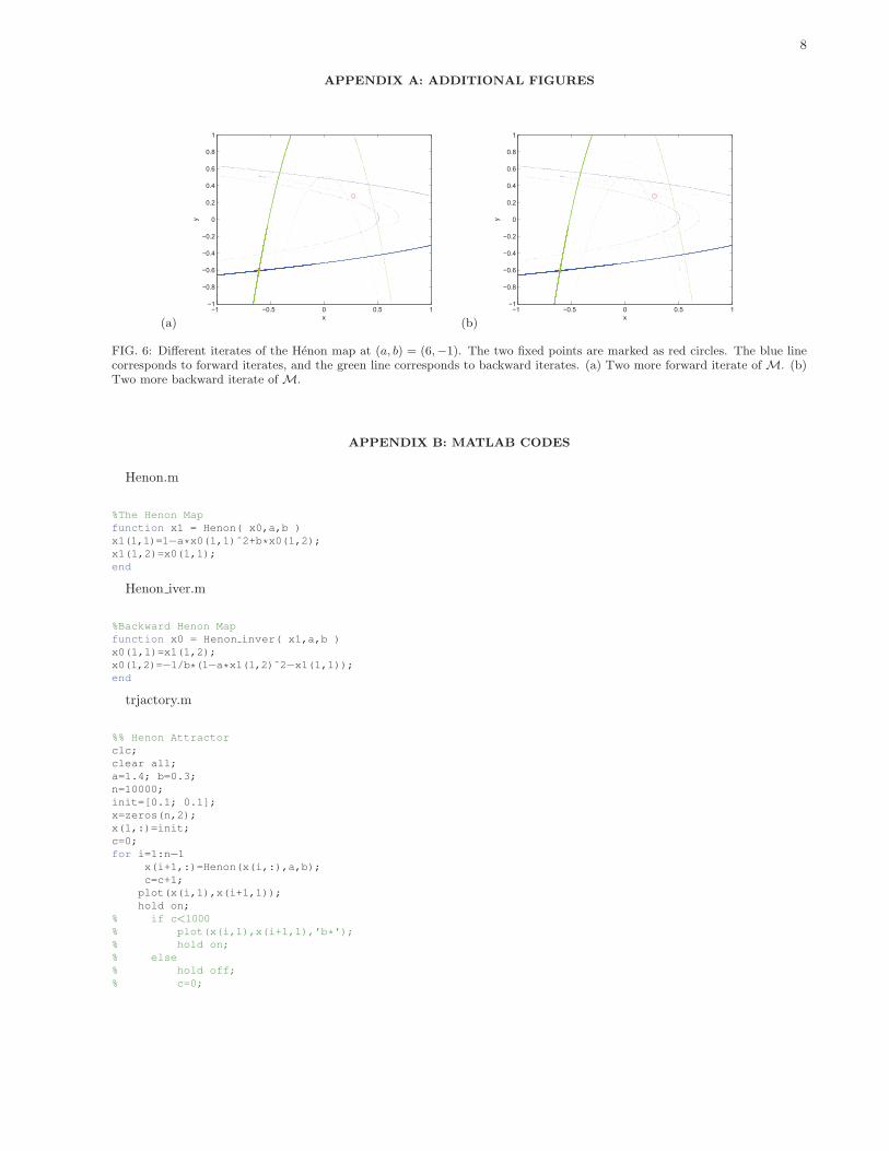
FIG. 6: Different iterates of the Henon map at (a, b) = (6,−1). The two fixed points are marked as red circles. The blue linecorresponds to forward iterates, and the green line corresponds to backward iterates. (a) Two more forward iterate of M. (b)Two more backward iterate of M.

APPENDIX B: MATLAB CODES

Henon.m

%The Henon Mapfunction x1 = Henon( x0,a,b )x1(1,1)=1−a*x0(1,1)ˆ2+b*x0(1,2);x1(1,2)=x0(1,1);end

Henon iver.m

%Backward Henon Mapfunction x0 = Henon inver( x1,a,b )x0(1,1)=x1(1,2);x0(1,2)=−1/b*(1−a*x1(1,2)ˆ2−x1(1,1));end

trjactory.m

%% Henon Attractorclc;clear all;a=1.4; b=0.3;n=10000;init=[0.1; 0.1];x=zeros(n,2);x(1,:)=init;c=0;for i=1:n−1

x(i+1,:)=Henon(x(i,:),a,b);c=c+1;plot(x(i,1),x(i+1,1));hold on;

% if c<1000% plot(x(i,1),x(i+1,1),'b*');% hold on;% else% hold off;% c=0;

9

% endendxlabel('x n');ylabel('x n + 1');

horseshoe.m

%% Henon Map Horseshoeclc;clear all;a=6; b=−1;x f1=(−(1−b)−sqrt((1−b)ˆ2+4*a))/(2*a);x f2=(−(1−b)+sqrt((1−b)ˆ2+4*a))/(2*a);n=10000;x0=x f1−0.01+0.02*rand(n,2);init step=4;forward=init step+1;backward=init step+1;for i=1:forward

for j=1:nx1(j,:)=Henon(x0(j,:),a,b);if x1(j,1)<1&&x1(j,1)>−1&&x1(j,2)<1&&x1(j,2)>−1

plot(x1(j,1),x1(j,2));hold on;

endendx0=x1;

endx0=x f1−0.01+0.02*rand(n,2);for i=1:backward

for j=1:nx 1(j,:)=Henon inver(x0(j,:),a,b);if x 1(j,1)<1&&x 1(j,1)>−1&&x 1(j,2)<1&&x 1(j,2)>−1

plot(x 1(j,1),x 1(j,2),'g');hold on;

endendx0=x 1;

endplot(x f1,x f1,'or',x f2,x f2,'or');xlabel('x');ylabel('y');