A Report on Putting Green PerformanceCharacteristicsMicah Woods, Ph.D.*

Chief Scientist | Asian Turfgrass Centerwww.asianturfgrass.com

August 2012

*I would like to thank all of the golf course superintendents, greenkeepers, coursemanagers, and friends who welcomed me to their golf courses during a busy time andwho not only allowed me to collect the data, but provided invaluable support in collectingthe data. I would also like to thank Mr. Yukio Ueno for translating this document intoJapanese.

1

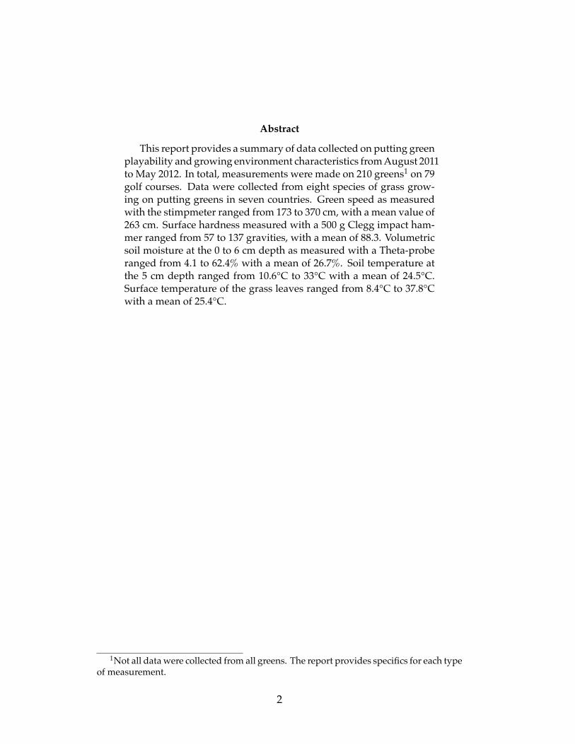
AbstractThis report provides a summary of data collected on putting green

playability and growing environment characteristics from August 2011to May 2012. In total, measurements were made on 210 greens1 on 79golf courses. Data were collected from eight species of grass grow-ing on putting greens in seven countries. Green speed as measuredwith the stimpmeter ranged from 173 to 370 cm, with a mean value of263 cm. Surface hardness measured with a 500 g Clegg impact ham-mer ranged from 57 to 137 gravities, with a mean of 88.3. Volumetricsoil moisture at the 0 to 6 cm depth as measured with a Theta-proberanged from 4.1 to 62.4% with a mean of 26.7%. Soil temperature atthe 5 cm depth ranged from 10.6°C to 33°C with a mean of 24.5°C.Surface temperature of the grass leaves ranged from 8.4°C to 37.8°Cwith a mean of 25.4°C.

1Not all data were collected from all greens. The report provides specifics for each typeof measurement.

2

Contents1 What data were collected, and why 4

2 Grass types 5

3 Data collected 5

4 Green speed 74.1 The Brede equation . . . . . . . . . . . . . . . . . . . . . . . . 7

5 Green hardness or firmness 135.1 Clegg hammer vs. Yamanaka tester . . . . . . . . . . . . . . . 17

6 Soil moisture 20

7 Soil and surface temperatures 20

8 Conclusion 24

3

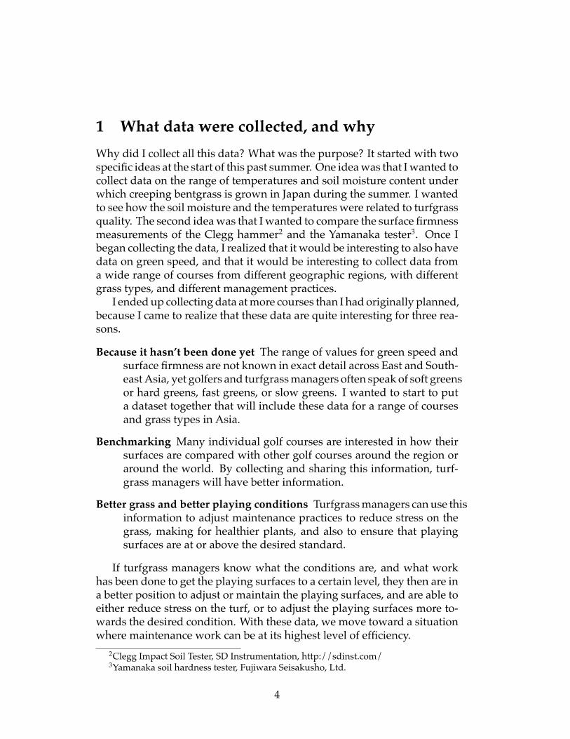
1 What data were collected, and whyWhy did I collect all this data? What was the purpose? It started with twospecific ideas at the start of this past summer. One idea was that I wanted tocollect data on the range of temperatures and soil moisture content underwhich creeping bentgrass is grown in Japan during the summer. I wantedto see how the soil moisture and the temperatures were related to turfgrassquality. The second idea was that I wanted to compare the surface firmnessmeasurements of the Clegg hammer2 and the Yamanaka tester3. Once Ibegan collecting the data, I realized that it would be interesting to also havedata on green speed, and that it would be interesting to collect data froma wide range of courses from different geographic regions, with differentgrass types, and different management practices.

I ended up collecting data at more courses than I had originally planned,because I came to realize that these data are quite interesting for three rea-sons.

Because it hasn’t been done yet The range of values for green speed andsurface firmness are not known in exact detail across East and South-east Asia, yet golfers and turfgrass managers often speak of soft greensor hard greens, fast greens, or slow greens. I wanted to start to puta dataset together that will include these data for a range of coursesand grass types in Asia.

Benchmarking Many individual golf courses are interested in how theirsurfaces are compared with other golf courses around the region oraround the world. By collecting and sharing this information, turf-grass managers will have better information.

Better grass and better playing conditions Turfgrass managers can use thisinformation to adjust maintenance practices to reduce stress on thegrass, making for healthier plants, and also to ensure that playingsurfaces are at or above the desired standard.

If turfgrass managers know what the conditions are, and what workhas been done to get the playing surfaces to a certain level, they then are ina better position to adjust or maintain the playing surfaces, and are able toeither reduce stress on the turf, or to adjust the playing surfaces more to-wards the desired condition. With these data, we move toward a situationwhere maintenance work can be at its highest level of efficiency.

2Clegg Impact Soil Tester, SD Instrumentation, http://sdinst.com/3Yamanaka soil hardness tester, Fujiwara Seisakusho, Ltd.

4

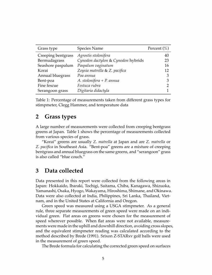
Grass type Species Name Percent (%)Creeping bentgrass Agrostis stolonifera 40Bermudagrass Cynodon dactylon & Cynodon hybrids 23Seashore paspalum Paspalum vaginatum 16Korai Zoysia matrella & Z. pacifica 12Annual bluegrass Poa annua 3Bent-poa A. stolonifera + P. annua 3Fine fescue Festuca rubra 2Serangoon grass Digitaria didactyla 1

Table 1: Percentage of measurements taken from different grass types forstimpmeter, Clegg Hammer, and temperature data

2 Grass typesA large number of measurements were collected from creeping bentgrassgreens at Japan. Table 1 shows the percentage of measurements collectedfrom various species of grass.

“Korai” greens are usually Z. matrella at Japan and are Z. matrella orZ. pacifica in Southeast Asia. “Bent-poa” greens are a mixture of creepingbentgrass and annual bluegrass on the same greens, and “serangoon” grassis also called “blue couch.”

3 Data collectedData presented in this report were collected from the following areas inJapan: Hokkaido, Ibaraki, Tochigi, Saitama, Chiba, Kanagawa, Shizuoka,Yamanashi, Osaka, Hyogo, Wakayama, Hiroshima, Shimane, and Okinawa.Data were also collected at India, Philippines, Sri Lanka, Thailand, Viet-nam, and in the United States at California and Oregon.

Green speed was measured using a USGA stimpmeter. As a generalrule, three separate measurements of green speed were made on an indi-vidual green. Flat areas on greens were chosen for the measurement ofspeed wherever possible. When flat areas were not available, measure-ments were made in the uphill and downhill direction, avoiding cross slopes,and the equivalent stimpmeter reading was calculated according to themethod described by Brede (1991). Srixon Z-STARxv golf balls were usedin the measurement of green speed.

The Brede formula for calculating the corrected green speed on surfaces

5

with a uniform slope less than 6% is

S =2ab

a+ b(1)

where,S = ball roll distance (corrected green speed)a = ball roll distance uphillb = ball roll distance downhill

Note that equation (1) is not the same as the standard equation (2) forcalculating ball roll distance which is the arithmetic mean of the uphill anddownhill direction, limited to a maximum difference between the two di-rections of 45 cm:

S =a+ b

2(2)

where,S = ball roll distancea = ball roll distance uphillb = ball roll distance downhill

In practice it is difficult to find flat areas on putting greens with a differ-ence of less than 45 cm in roll, and thus the Brede formula is quite useful.All green speeds in this report, unless otherwise noted, were calculatedusing equation (1).

Green firmness was measured using a Clegg hammer from SDi with a500 g domed end probe (golf probe). Nine readings were taken from eachgreen, with one reading being a single drop of the hammer through a guidetube from a height of 60 cm. Readings are a measurement of the peak de-celeration of the hammer’s impact with the surface and are given in unitsof gravities, represented in this report as Gmax. Whenever possible, read-ings at the same location on the green were also made with a Yamanakasoil hardness tester, and those results are in mm and correspond to a forcein kg cm-2.

Soil moisture to a depth of 6 cm was measured with a Theta-probe fromDelta-T Devices4. Nine readings were made per green, generally in a loca-tion close to the Clegg hammer readings.

Soil temperatures were measured at three locations on each green with4Theta-probe, Delta-T Devices, http://www.delta-t.co.uk/

6

a digital thermometer5 inserted to a 6 cm depth. Surface temperatures weremeasured with an infrared thermometer6, held at approximately 50 cmabove the green surface to measure the integrated temperature of a circleon the green surface approximately 5 cm in diameter.

Data were analyzed using R software (R Development Core Team, 2012),graphs were generated by the ggplot2 package (Wickham, 2009), and theEnglish version of this report was generated by the knitr package (Xie,2012) with final typesetting done in X ELATEX.

4 Green speedFigure 1 shows all the measurements of green speed. Of the 623 measure-ments, there was a range from 173 to 370 cm, with a mean value of 263 cm.Table 2 shows the equivalent speed in feet and inches for the range of greenspeeds discussed in this report.

The boxplots in Figure 1 show the distribution of the data collected foreach grass type. The horizontal line at the center of the boxplot for eachspecies is the median green speed for that grass species. Each individualpoint represents one measurement of green speed, with its value on thex-axis corresponding to the species of grass, and the value on the y-axisshowing the green speed calculated through equation (1) for that measure-ment.

Data for creeping bentgrass, bermudagrass, seashore paspalum, andkorai were all collected from eight or more different golf courses. Data forbent-poa, fescue, Poa annua, and serangoon grass were all collected fromthree or fewer golf courses. We can look at the data for the first set ofgrass species as being somewhat representative of the species. The datafor the second set of species, taken from a limited number of sites, may bemore representative of the maintenance practices used at the golf coursesfrom which the data were collected, rather than an indication of the normalrange for the species.

4.1 The Brede equationThe Brede equation (1) is extremely useful. On most golf course puttinggreens, it is difficult to find flat areas to make a stimpmeter reading. In thisproject, I collected green speed data from 210 greens and even in places

5Taylor Precision Products model 9842 waterproof digital thermometer,http://www.taylorusa.com/

6Fluke 62 mini infrared thermometer, http://www.fluke.com/

7

Speed (cm) Speed (feet)170 5’7”180 5’11”190 6’3”200 6’7”210 6’11”220 7’3”230 7’7”240 7’10”250 8’2”260 8’6”270 8’10”280 9’2”290 9’6”300 9’10”310 10’2”320 10’6”330 10’10”340 11’2”350 11’6”360 11’10”370 12’2”

Table 2: Green speed in cm shown with the equivalent in feet

8

200

250

300

350

bent bent−poa bermuda fescue korai paspalum poa serangoonSpecies

Gre

en S

peed

(cm

)

Figure 1: 617 measurements of green speed, separated in boxplots for eachspecies

9

0

100

200

0 200 400 600 800Difference in roll distance (cm) between uphill and downhill direction

Err

or in

gre

en s

peed

(cm

), c

alcu

late

d by

US

GA

equ

atio

n −

Bre

de e

quat

ion

Figure 2: Error in stimpmeter readings increases rapidly when the differ-ence between the two roll directions is more than 45 cm

10

where the green seemed to be relatively flat, the difference in roll betweenthe uphill and downhill direction was often more than 45 cm. When greenspeed readings are made, a location at the edge or corner of a green is of-ten selected, not because it is a representative area of the green, but simplybecause that corner or ridge is flat enough to get a valid reading. Alter-natively, slightly sidehill rolls are sometimes made, so that the differencebetween the two rolls is less than 45 cm, even though the sidehill roll causesa curve that introduces error into the reading.

In Figure 2 we see the error that comes into the stimpmeter readingwhen measurements are made on a slope such that the difference in rollbetween the uphill and downhill direction is more than 45 cm. The blueline marks the 45 cm breaking point. With a difference less than 45 cmbetween the two directions, equation (2) can be used. With any differencegreater than 45 cm, the error in the reading is too great, and we cannotmake a stimpmeter reading using the standard method.

But wouldn’t it be great if we could obtain an accurate stimpmeter mea-surement on sloped areas where the difference in roll between the uphilland downhill direction is more than 45 cm? Figure 3 shows that we can dothat by using the Brede equation (1).

By making multiple measurements of green speed on each green, thedata can be organized to compare the green speed within greens. Figure 3shows that for each of those paired measurements, meaning two measure-ments taken at different locations on the same green, the speed on thesloped area, even when the difference in roll between the uphill and thedownhill direction was 500 cm, once corrected using equation (1), was ableto predict accurately the speed measured at a flat (difference between up-hill and downhill < 45 cm) location on that same green. In effect, the resultof the Brede equation is to remove the error that was shown in Figure 2.

What about that scatter around the 1:1 line in Figure 3? Is that normal,or should we expect that two measurements from the same green shouldalways have exactly the same value? If the stimpmeter reading is identicalat the two paired areas, it would be shown in Figure 3 right on top of theblue 1:1 line. What we see in the figure is a little bit of scatter around thatline, both for the sloped vs. flat measurements (in orange) and the flat vs.flat measurements (in blue).

Even within one green, it is natural that the speed varies somewhatfrom point to point. Just because we measure a stimpmeter reading of acertain value at the back of the green, it does not mean that the front of thatgreen, or the middle of that green, will be exactly the same speed. To inves-tigate this in more detail, I compared paired measurements from two flatareas on the same greens (n = 36). I also compared paired measurements

11

200

250

300

350

200 250 300 350Predicted green speed from Brede equation (cm)

Act

ual g

reen

spe

ed fr

om p

aire

d re

adin

g on

sam

e gr

een

in fl

at a

rea

(cm

)

Predictor(x−axis)differencein cm(downhill− uphill)

0

100

200

300

400

500

Figure 3: 212 paired measurements of green speed shown in orange use themeasurement from a sloped area (x-axis value) to predict the green speedfrom a flat area (roll difference < 45 cm) on the same green; 36 paired mea-surements of green speed shown in blue use the green speed of a flat areato predict the green speed of another flat area on the same green; the size ofthe circles on the graph represent the difference in roll distance between theuphill and downhill direction for the predictor green speed on the x-axis

12

of a sloped area with a flat area on the same green (n = 212).In the paired measurements of two flat areas on the same green, the

median difference between stimpmeter readings was 9. In the paired mea-surements of a sloped area to a flat area on the same green, the mediandifference between stimpmeter readings was 9.9. Based on these results, Iwould expect that on a typical green, the difference in speed from one areato the next may be about 9 cm. And it appears that including measure-ments from sloped areas only introduces additional variability of about 1cm.

To put this variability into context, Karcher et al. (2001) demonstratedthat golfers are not able to detect a difference in green speed of less than15 cm. Repeated measurements of green speed on the same research plotsfound variability among stimpmeter measurements to be less than 15 cm(Richards et al., 2009) with that variability being attributed to factors suchas varying wind speed and direction, non-uniform surface conditions, anddifferences in leaf blade orientation due to grain or mowing patterns.

A look at the probability density functions (Figure 4) for the sloped vs.flat measurements (orange) and for the flat vs. flat measurements (blue)shows a lot of overlap, although the flat vs. flat measurements have fewerdifferences above 20 cm. For practical purposes, the distribution of thedifferences between the paired stimpmeter readings are similar, suggest-ing that use of the Brede equation (1) on sloped areas of a green produces astimpmeter reading that is functionally equivalent to the stimpmeter read-ing on a flat area of the same green.

5 Green hardness or firmnessThe hardness of the putting surface is another important performance char-acteristic. Baker et al. (1996) used a 500 g Clegg hammer to measure thesurface hardness of 148 greens on 74 golf courses in Great Britain. Theirmeasurements of Gmax mostly fell within the range of 70 to 150; on greensless than five years old the mean Gmax was 126, with that value decreas-ing to 108 for courses ten or more years old. Figure 5 shows a histogramof the 2029 measurements I made of Gmax. The most frequent measure-ments were from 80 to 90, and the range was from 57 to 137 with a meanof 88 gravities.

Figure 6 shows a boxplot of all the Gmax measurements, separated byspecies. We notice that the warm-season grasses tend to have harder sur-faces than do the cool-season grasses, although there is a wide range forall species at which data were collected at more than one course. Data for

13

0.00

0.01

0.02

0.03

−25 0 25 50Difference between paired stimpmeter readings on the same green (cm)

dens

ity

Figure 4: In orange, the probability density function for the difference in212 paired measurements of Brede equation measurements from slopedareas and a measurement from a flat area on the same green; in blue, theprobability density function for the difference in 36 paired measurementsof stimpmeter readings from two flat areas on the same green

14

0

100

200

300

400

50 75 100 125Gmax

Cou

nt

Figure 5: Histogram of 2029 Clegg hammer measurements of hardness(Gmax) on putting greens

15

60

80

100

120

140

bent bent−poa bermuda fescue korai paspalum poa serangoonSpecies

Cle

gg H

amm

er (

Gm

ax)

Figure 6: Clegg hammer measurements of green hardness (Gmax), sepa-rated in boxplots for each species

16

bent-poa, fescue, poa, and serangoon grass should be evaluated with carein comparing to other species because those data were collected from asmall set of courses, thus the data may represent more about the manage-ment of the turf at those courses than about the grass species itself.

I find it interesting that seashore paspalum greens tended to be firmerthan did bermudagrass greens. This is probably because seashore pas-palum greens tend to be newer, thus probably having less organic matterin the soil, and consequently would be firmer. The korai greens tended tobe softer, and I suspect this is for three reasons:

1. Korai greens tend to be older than bermuda or seashore paspalumgreens, thus having more organic matter in the soil

2. Korai is a particularly well-adapted grass to East and Southeast Asiawhere data were collected, so we expect that the grass may naturallyproduce a large amount of organic matter compared to other grassesin this type of climate

3. It is rare that korai greens receive as much maintenance as do greensplanted to another species

We saw in Figure 1 that the speed of korai greens can match the speedof other warm-season grasses; the data in Figure 6 show that korai greenstend to be softer than those of other warm-season grasses. But korai greenstend to receive less maintenance than other grasses. How good can koraigreens be, especially in Southeast Asia, with increased frequency of sandtopdressing and increased use of growth regulators? Based on these dataand the surprisingly high average green speed of korai, the answer maybe “surprisingly good”.

5.1 Clegg hammer vs. Yamanaka testerAt Japan the Yamanaka soil hardness tester is often used to measure thefirmness of a green. One of the objectives of this study was also to evaluatethe relationship between the Clegg hammer and the Yamanaka tester.

Figure 7 shows the scatterplot of Clegg and Yamanaka data taken fromthe same points. This is a rather small dataset, representing 39 greens, 8courses, and 345 paired measurements, in total. There is more sensitivity tochanges in surface hardness when measured with the Clegg hammer thanwhen measured with the Yamanaka tester. The range of measurements in345 samples was only 9, from a low of 16 to a high of 25, for the Yamanaka

17

18

20

22

25

70 80 90 100 110 120Clegg Hammer (Gmax)

Yam

anak

a Te

ster

(m

m)

Figure 7: Scatterplot of Clegg hammer and Yamanaka tester, with the blueline showing the mean value of the Yamanaka tester for any value of Gmax

18

tester. With the Clegg, there was a range of 48 units, from a low of 71 to ahigh of 119.

We see in Figure 7 that there is a lot of scatter in the middle of the plot.When Gmax is in the range from 80 to 100, which we saw in Figure 5 rep-resents the typical green condition, there is very little correlation betweenthe Clegg hammer reading and the Yamanaka tester reading.

0.0

0.2

0.5

0.8

1.0

70 80 90 100 110 120Clegg Hammer (Gmax)

Den

sity

, sca

led

to 1

0.0

0.2

0.5

0.8

1.0

18 20 22 25Yamanaka Tester (mm)

Den

sity

, sca

led

to 1

These small plots show a scaled probability density function for theClegg hammer and Yamanaka tester data. The Clegg hammer at left is inyellow and the Yamanaka tester data is in white at right. The curve for theClegg hammer data are wider, indicating more sensitivity in the measure-ments, while the data for the Yamanaka tester are more closely clusteredaround the values of 20, 21, and 22. For greens that are quite soft, or greensthat are quite hard, the Yamanaka tester captures that information. In themiddle range of green firmness, however, this limited comparison of the

19

Clegg hammer and the Yamanaka tester suggests that the Gmax data froma Clegg hammer would be more sensitive to the variability in surface hard-ness.

6 Soil moistureThere were 1193 measurements of soil moisture, representing most but notall of the grasses tested. Figure 8 summarizes the soil moisture content ina boxplot by species. We note that bermuda and korai had the lowest av-erage soil moisture content, which is what we would expect; warm seasongrasses use water more efficiently than do cool season grasses and thuscan be maintained at lower levels of soil moisture. It is interesting to notethat the mean of all the 1193 soil moisture measurements was 26.7%. Thesedata were collected, overwhelmingly, from sand-based USGA rootzones.The USGA recommendations for putting green construction (United StatesGolf Association Green Section Staff, 2004) specify a capillary porosity atconstruction of 15 to 25%. On average, the greens that I tested were at orabove that level.

There is some indication that soil moisture content has an influence onsurface hardness. Figure 9 shows that there are hard greens associated withlow moisture content and soft greens associated with soil moisture contenthigher than 35%. Above 35% soil moisture, turfgrass managers may losethe ability to keep surfaces at a firm level of 100 (Gmax) or above.

7 Soil and surface temperaturesFigure 10 summarizes the temperatures by country, with surface tempera-tures measured at the time I collected the data shown as green circles, andthe soil temperatures at the time I collected data shown as orange triangles.There are obviously a lot of seasonal variations in these temperatures, atleast in temperate countries. At Thailand the temperatures near sea levelare relatively consistent throughout the year.

It is interesting to note that in Japan, at the hottest time during the sum-mer, the surface temperatures and soil temperatures equal or exceed thetemperatures measured at tropical locations in Thailand, the Philippines,and Sri Lanka.

20

20

40

60

bent bent−poa bermuda korai paspalum poaSpecies

Vol

umet

ric W

ater

Con

tent

(%

)

Figure 8: Volumetric soil water content in the top 6 cm of the soil, measuredat 1193 points on golf course putting greens, separated in boxplots for eachof the six species from which data were collected

21

60

80

100

120

140

20 40 60Volumetric Water Content (%)

Cle

gg H

amm

er (

Gm

ax)

Figure 9: The relationship between soil moisture content measured to a6 cm depth and surface hardness for 1193 paired samples on golf courseputting greens of multiple species

22

10

20

30

India Japan Philippines Sri Lanka Thailand USA VietnamCountry

Soi

l (or

ange

tria

ngle

) or

Sur

face

(gr

een

circ

le)

tem

pera

ture

(°C

)

Figure 10: Soil temperature at a 6 cm depth and surface temperature for allthe greens from which data were collected

23

8 ConclusionThe collection of these data and the preparation of this report turned into amuch larger and longer project than I had anticipated. This larger project,however, is a more useful one than what I set out to do looking at soil andsurface temperatures of some golf course greens in Japan during the sum-mer. For that, I am indebted to the many friends who helped me to collectthis data and to the Golf Course Committee of The R&A who provided oneof the meters used in this study.

These data, with which I have been wrangling for untold hours, havecertainly helped me to learn more about putting green performance andsome of the playability characteristics for different grass species and in dif-ferent countries. I’ve prepared this report in an attempt to provide a basicsummary of the data, to show where the data from your course lie in re-lation to all the other data I collected, and in a few cases, to show some ofthe things that I think are really interesting (like the Brede equation!) andto delve into those data in more detail.

I hope you will have found these data as interesting as I have and thatthis information can be of some use to you in the management of yourfacility.

ReferencesS.W. Baker, P.D. Hind, T.A. Lodge, J.A. Hunt, and D.J. Binns. A survey of

golf greens in Great Britain. IV. playing quality. J. Sports Turf Res. Inst.,72:9–21, 1996.

A.D. Brede. Correction for slope in green speed measurement of golf courseputting greens. Agronomy Journal, 83:425–426, 1991.

D. Karcher, T. Nikolai, and R. Calhoun. Golfer’s perceptions of greenspeeds vary: over typical stimpmeter distances, golfers are only guess-ing when ball-roll differences are less than 6 inches. Golf Course Manage-ment, 69(57-60), 2001.

R Development Core Team. R: A Language and Environment for StatisticalComputing. R Foundation for Statistical Computing, Vienna, Austria,2012. URL http://www.R-project.org. ISBN 3-900051-07-0.

Jacob S. Richards, Douglas E. Karcher, Thomas A. Nikolai, Jason J. Hen-derson, and John C. Sorochan. A comparison of two devices used to

24

measure golf course putting green speed. Applied Turfgrass Science, on-line(doi:10.1094/ATS-2009-0724-02-RS), 2009.

United States Golf Association Green Section Staff. USGA recommenda-tions for a method of putting green construction. USGA World WideWeb Site, March 2004.

Hadley Wickham. ggplot2: elegant graphics for data analysis.Springer New York, 2009. ISBN 978-0-387-98140-6. URLhttp://had.co.nz/ggplot2/book.

Yihui Xie. knitr: A general-purpose package for dynamic report generation inR, 2012. URL http://CRAN.R-project.org/package=knitr. Rpackage version 0.5.

25