Are Under- and Over-reaction the Same Matter? A Price Inertia based Account∗ Shengle Lin and Stephen Rassenti Economic Science Institute, Chapman University, Orange, CA 92866, USA Latest Version: Nov, 2008 Abstract. Theories on under- and over-reaction in asset prices fall into three types: (1) they are respectively driven by different psychological factors; (2) they are driven by different types of investors; and (3) they reflect un-modeled risk. We design an asset market where information arrives sequentially over time and is revealed asymmetrically to investors. None of the three hypotheses is supported by our data: (1) Investors do not respond differently to public information and private information, and they do not behave in ways that are claimed by multiple psychological models; (2) no groups of investors are identified to drive under- or over-reaction in particular; (3) price deviation from expected payoff cannot be justified by risk metrics. We find that prices react insufficiently to news surprises, possibly because of cautious conservatism on the part of investors and under-reacting drifts outnumber overreacting reversals substantially. Contrary to common beliefs, we find that over-reaction is caused by slow adjustment of prices to surprises, similar to the cause of under-reaction. It is the degree of price inertia that drives the relative frequencies of under- and over-reaction. We propose a simple price inertia theory of under- and over-reaction: when information arrives sequentially over time, the market is characterized by a slow convergence toward intrinsic value; when news surprises are of the same signs, prices falls behind newly updated intrinsic values, manifesting under-reacting drifts; when news surprises change signs, prices again do not adjust quick enough to catch up with the new intrinsic values, manifesting a temporal pattern of overreacting reversals. JEL classification: C92; D53; G14 KEYWORDS: Experimental finance, under-reaction, overreaction, behavior, price inertia, risk aversion

                                                            

∗ Financial Support was provided by the International Foundation for Experimental Economics and Economic Science Institute of Chapman University. We thank Vernon Smith, David Porter and participants at Brownbag talk series of Economic Science Institute. The paper benefited from comments at numerous seminars and meetings in America. Correspondence to: slin@chapman.edu

Are Under- and Over-reaction the same matter? A Price Inertia based Account Abstract. Theories on under- and over-reaction in asset prices fall into three types: (1) they are respectively driven by different psychological factors; (2) they are driven by different types of investors; and (3) they reflect un-modeled risk. We design an asset market where information arrives sequentially over time and is revealed asymmetrically to investors. None of the three hypotheses is supported by our data: (1) Investors do not respond differently to public information and private information, and they do not behave in ways that are claimed by multiple psychological models; (2) no groups of investors are identified to drive under- or over-reaction in particular; (3) price deviation from expected payoff cannot be justified by risk metrics. We find that prices react insufficiently to news surprises, possibly because of cautious conservatism on the part of investors and under-reacting drifts outnumber overreacting reversals substantially. Contrary to common beliefs, we find that over-reaction is caused by slow adjustment of prices to surprises, similar to the cause of under-reaction. It is the degree of price inertia that drives the relative frequencies of under- and over-reaction. We propose a simple price inertia theory of under- and over-reaction: when information arrives sequentially over time, the market is characterized by a slow convergence toward intrinsic value; when news surprises are of the same signs, prices falls behind newly updated intrinsic values, manifesting under-reacting drifts; when news surprises change signs, prices again do not adjust quick enough to catch up with the new intrinsic values, manifesting a temporal pattern of overreacting reversals. JEL classification: C92; D53; G14 KEYWORDS: Experimental finance, under-reaction, overreaction, behavior, price inertia, risk aversion

2

1. Introduction Numerous theories against the efficient market hypothesis (Fama, 1978), have

attempted to reconcile empirical findings concerning under and over-reaction of asset prices to significant information events. The purpose of this study is to test how robustly these competing theories hold up in laboratory markets where the temporal and spatial distribution of information can be precisely controlled. Experience with asset markets both in the field and the laboratory suggests that human investors behave in a more complicated and strategic manner than in any ad hoc models or simulations so far constructed.

Empirical results on asset price responses to news events seem to support systematic under-reaction in which average post-event returns hold the same sign as pre-event date returns (Jagadeesh and Titman, 1993)1. Meanwhile, numerous studies conversely note that investors can over-react causing price movement featuring disproportional price changes followed by subsequent reversions (DeBondt and Thaler, 1985) 2. The anomalies literature tends to suggest that in the short to medium run, returns appear to exhibit continuation, while over-reacting return reversals are more likely to occur in the long run. In either case, price adjustments are considered to be biased.

The anomalies literature has assembled abundant counter-evidence to challenge market efficiency hypotheses, but not provided a unifying alternative theory. Fama (1998) points out that even though market efficiency is “a faulty description of price formation”, the alternative hypotheses are “vague” and rarely tested: this he deems as “unacceptable”. In other words, any alternative must also be tested to prove that it outperforms market efficiency theory’s prediction that the expected value of abnormal returns is zero, and that deviation from zero in either direction can solely be attributed to chance.

In this study, we address three distinct lines of approaches. The first approach advocates that the price reaction to news events is determined by psychological beliefs of an aggregate agent, including the overconfidence and self-attribution model by Daniel,

                                                            

1 Jagadeesh and Titman (1993) argue that under-reaction is the cause for the success of momentum investing. Bernard and Thomas (1990), and many others, have documented drift after earnings surprises for up to 12 months after the initial surprise. Ikenberry, Lakonishok, and Vermaelen (1994) contend that the market phase of under-reaction is an important motive for stock repurchase. Ikenberry and Ramnath (2002) found evidence that the pattern even persists in stock splits, which is the simplest corporate event. Abarbanell and Lehavy (2003) found that analysts’ forecasting errors are correlated with the reporting choice a corporation makes in announcing its unexpected accruals. Mikhail, Walther, and Willis (2003) demonstrated that the analysts’ under-reaction to corporate announcements tends to decrease with the years of experience that they follow the firm. 2 DeBondt and Thaler (1985) find that “loser” portfolios experience exceptionally large January return as late as five years after the initial portfolio formation. DeBondt and Thaler (1987) find that there exists mean reversion in stock returns, and excess return to losers could be explained by a biased expectation of the future which over weighs recent information and under weighs the long term average. DeBondt and Thaler (1990) find that security analysts’ forecasts are overoptimistic and exhibit frequent revisions. Dreman and Lufkin (2000) argue that the profitability of contrarian strategies results from the existence of over-reaction and that psychological factors may explain the origin of over-reaction. 

3

Hirshleifer and Subrahmanyam (1998, hereafter DHS), the conservatism and representative bias by Barberis, Shleifer and Vishny (1998, hereafter BSV) and the disposition effect model by Frazzini (2006). The second approach advocates that the types of reactions are driven by different groups of investors, featuring the information transmission model with heterogeneous agents by Hong and Stein (1998, hereafter HS). These two approaches both regard under- and over-reaction as two distinct phenomena. The third approach features Fama’s (1998) risk-based explanation, arguing that under- and over-reaction is purely a reflection of risk that are not captured by asset pricing models.

Our laboratory test utilizes the model presented in HS (1999) to generate the asset valuation process experienced by investors. The asset pays a liquidation value to its owner when time reaches maturity with its book value unit is subject to a series of surprises during its lifetime and information in each period available for the informed to compute the expected liquidation value, i.e. intrinsic value. Common knowledge amongst investors exists about the underlying process and the ultimate state-dependent payoff, and also concerning a periodic structure of information release. Public information disseminates instantaneously throughout the population, while private information reaches only a subgroup of insiders. Information is both dispersed over time and asymmetrically throughout the investor population, generating a process of HS (1999) information diffusion.

We identify under- and over-reaction with the advantage of knowing perfectly the intrinsic values. Our methodology reveals under-reaction as the predominant short-term and long-term regularity in most markets. To demonstrate the necessity of knowing the intrinsic value, we also use the traditional return sign characterization to sort our data and confirm the worry that observed anomalies can be created by researchers ignorant of intrinsic value. When taking intrinsic value into account, we find that the traditional continuation/reversal of returns signs does not consistently indicate true under/over-reaction, as it may easily be misinterpreted absent the knowledge of intrinsic value.

Our experimental results demonstrate that: (1) Data do not support psychological based explanations, either over-confidence

model or disposition effect model; (2) Underreaction and overreaction are not caused by different groups of investors.

In particular, HS' information transmission model cannot explain the drift pattern of prices;

(3) Risk cannot account for drifts; overpricing or under-pricing cannot be captured by risk-return relationship;

(4) Adjustment to surprises is robustly insufficient and displays inertia. The inferred aggregate subjective probabilities displayed by these markets indicate that biased judgments tend to persist and that the markets exhibit belief continuation. The ‘conservatism’ account of BSV is the sole model that best governs the inertia patterns among all testable theories.

In addition, we find that over-reaction is also caused by cautiously conservative

adjustments. No theory has ever linked cautiousness with overreacting behaviors. We

4

hypothesize that over-reaction is just a by-product of cautiousness as well, and under- and over-reaction are categorized differently simply because of the difference in historical price positions relative to the intrinsic value. This is not so surprising, since mispricing, either over or under, would always be determined by the path in the intrinsic value. By carefully re-examining the overreaction cases in our data, we confirm that overreaction, either changing from under-pricing to over-pricing or changing from over-pricing to under-pricing, is mostly caused by prices falling behind the abrupt changes in the intrinsic value.

To test the price inertia theory more generally, we run numeric simulations using parameters derived from the laboratory data. Without introducing anything other than short-term insufficient adjustment, a substantial level of overreaction (persistent return reversal) emerges: the source for this apparent overreaction is also that prices do not converge fast enough to track abrupt changes in intrinsic value, resulting in a turning in price direction. The more inadequate the adjustments to the changes in intrinsic value are, the more under-reaction patterns will prevail. We confirm that short term insufficient adjustment can be the sole driving factor in determining the under- and over-reaction regularities. Both instances are governed by how responsively the market prices adjust to information events, rather than driven by contrasting behavioral traits or the interaction of heterogeneous market participants.

We conclude that informational efficiency cannot be fully described by any single theory surveyed in this paper. We argue that both short-run return continuations (driven by slow adjustment) and long-run return reversals (possibly the slow re-adjustments to the new intrinsic value) can be summarized as manifestations of inertia, and that the theoretical dichotomy between under-reaction studies and over-reaction studies can be inherently misleading.

The rest of the paper is organized as following. Section 2 surveys some prominent existing theoretical models that attempt to explain empirical data. Section 3 specifies the experimental design we devised for the laboratory markets and states the testable hypotheses relating to the various theoretical models. Section 4 presents our data summary. Section 5 evaluates the validities of the five competing models and presents our simulation results. Section 6 proposes a price inertia based theory of under- and over-reaction. Section 7 summarizes our findings briefly.

2. Theories on Under- and Over-reaction A number of theoretical models have attempted to provide partial or ‘unified’

explanations for either under or over-reaction, or both regularities. The first approach features the defense of the efficient market hypothesis.

2.1 Psychological Explanations The first approach features various models of investor psychology. DHS (1998) develop a model of investor overconfidence, examining how investors

assimilate new information. The uninformed investors are not subject to judgment bias

5

and prices are determined by the informed investors. The model argues that informed investors are “overconfident” about the information they privately own, and as a result, overreact to this type of information. In addition, a second characteristic named “biased self-attribution” reinforces their over-confidence whenever public information is in agreement with their private signal. When public information is not in accordance with their private signal, biased self-attribution leads to dismissal of the information as noise. The model suggests that the market under-reacts to public information and over-reacts to private information so the responses produce short-term continuation of returns and long-term reversals as public information eventually overwhelm the behavioral biases.

BSV (1998) proposed a model known as a “conservatism bias” 1 (attributed to Edwards (1968)) which essentially means that individuals tend to underweight new information when updating their prior beliefs. Conservatism bias leads investors to update their beliefs very slowly in the face of new evidence. “Representativeness bias”, on the other hand, leads to the formation of biased estimates based on a small sample of observations. In the BSV model, the earnings follow a random walk but investors falsely perceive that there are two earning regimes. In regime A, earnings are mean-reverting and in regime B, earnings are trending. If investors believe regime A holds, price under-reacts to changes in earnings because investors mistakenly think the change is likely to be temporary; if investors believe regime B holds, they incorrectly extrapolate the trend and the price over-reacts. Overall, investors form prior beliefs about future prospects and the prior beliefs carry over to future price formation.

Frazzini (2006) proposes that the presence of “disposition effect” 2 , initiated by Shefrin and Statman (1985), will depress prices following good news as investors rush to sell to lock in paper gains, and will halt prices from falling following bad news as investors are reluctant to sell absent a premium. The former would lead to higher subsequent returns while the latter would lead to lower subsequent returns. Therefore, the disposition effect posits that a past capital gain or loss will shape the subsequent price formation, a unique explanation for asset price under-reaction.

2.2 Heterogeneous Investors The second theoretical approach focuses on the market microstructure. Hong and

Stein (HS, 1999) hypothesize that the market contains two groups of investors who trade based on different strategies. Informed investors base their trades on private signals about future cash flows while technical investors base their decisions on a limited history of prices. Information obtained by informed investors is transmitted slowly into the market, leading to an under-reaction pattern in returns. Technical investors rely on the past history of prices and extrapolate the trend too far, reinforcing momentum and pushing price away from intrinsic value which leads to an eventual reversal in returns. No                                                             

1 See Richards Heuer, Jr., Psychology of Intelligence Analysis, Central Intelligence Agency, 1999. He wrote: “As a general rule, people are too slow to change an established view, as opposed to being to willing to change. The human mind is conservative. It resists change.” 2 This is a behavioral tendency on the part of investors to hold onto their losing stocks to a greater extent than they hold onto their winners. (Shefrin and Statman, 1985). O’dean (1998) and Grinblatt and Han (2005) modeled or documented evidences that investors2 indeed rush to sell after capital gains and are reluctant to sell after capital loss. 

6

assumption on the limitations of psychology is made. HS posit that information aggregation failure leads markets to under-react, and consequently, this under-reaction will be more pronounced when information updates have higher asymmetry (Hong, Lim and Stein, 2001). On other hand, HS model implies that prices will extrapolate trends and move to overshooting levels due to momentum trading actitivies.

2.3 Risk based Explanation Fama (1998) presents three reasons for keeping market efficiency as a viable

working model. First, the literature does not present a random sample of events and pays more attention to splashy results. Second, some apparent anomalies arise due to risk premium that are not captured by existing asset pricing models. The empirical evidence concerning observed investor mis-reactions can be the result of poorly specified risk factor models, with some effects disappearing entirely after accounting for size and book-to-market ratio effects (Fama and French, 1996). Third, Fama (1998) surveys the anomalies literature and finds an even split between evidence for over-reaction and under-reaction and contends that long term efficiency is likely to hold up. The argument poses powerful skepticism upon the literature as there has long been absent a robust asset-pricing model.

Empirical tests of these theories face multiple challenges in data collection. Firstly, the observed anomalies may well reflect changes in the fundamentals that are never known for certain but at best inferred. Secondly, the absence of a robust risk pricing model may depict the market’s rational response to changes in risk factors as improper reactions, an issue Fama (1998) referred to as the “bad-model problem”. And thirdly, it is hard to draw a distinction between public information and private information, as information leakage to insiders before public declaration cannot easily be detected. A laboratory controlled asset market is able to fully satisfy these difficult data requirements and offers a new approach to disentangling the impasse. Smith (1982) formalizes the notion of an economic system by specifying three constituent components: environment, institution, and behavior. In the laboratory all environmental parameters and institutional rules are perfectly controlled, thus providing a perspective that is impossible to obtain in the field.

3. Experimental Design Our design adopts the HS (1999) information diffusion model in a multi-period

exchange economy where information updates are temporally dispersed and asymmetrically held. Both the DHS and BSV models have a similar multi-period structure allowing long term behavior to emerge. Investors trade from period 1 until period 10 and receive a liquidation value per asset held after period 10 trading is complete. In each period either a specific subset of investors or all investors receive information concerning the assets’ liquidation value. There are no supply shocks in the market that may prevent equilibrium prices from fully revealing the investors’ private information. The structure of this economy is common knowledge.

7

3.1. The Random Walk Model Each investor is endowed with a portfolio of cash and a risky asset. The cash

account may be regarded as a riskless bond, and for simplicity we normalize its interest rate to zero. The risky asset in the market pays a liquidation value of at the end of period

TDT , which is imperfectly known to investors at all times prior to the end of

periodT . The liquidation value is determined by two components: a known starting book value, , plus a series of news surprises, each directly affecting the current book value, with one surprise between each consecutive pair of trading periods. Therefore, the book value of the asset as we proceed through time follows a symmetric binomial random walk:

1D

TtDD ttt ,,3,2,1 L=+= − ε (1)

Thus, for any period t (after period 1), the book value is:

TtDDt

iit ,,3,2,

21 L=+= ∑

=

ε (2)

In HS, tε is randomly generated by a mean zero 1 normal distribution. The

distribution for each surprise in our design is simplified to a binomial draw:

Ttpd

pu

t ,,3,25.0)1(,

5.0,K=

⎪⎩

⎪⎨⎧

=−−

=+=ε (3)

The surprises are independently and identically distributed. If a positive surprise

occurs, a definite amount of money, u will be added to the asset’s current book value; if a negative surprise occurs, a definite amount of money, d will be subtracted from the asset’s current book value. There is a 50/50 chance of each outcome2. Just before the final periodT , the final surprise is revealed and the liquidation value is ascertained.

                                                           

We set , so each session lasts for 10 trading periods. The above model creates a binomial process in the intrinsic asset value. The following descriptive statistics can be obtained.

10=T

 

1 Our parameters for all market sessions sum to a mean zero distribution. In individual market sessions, the parameters can have negative, positive or zero mean. 2 The content of information released to investors can be structured either to change the probabilities related to the state-dependent payoffs, or to change the payoffs (book value) directly. Generally, values are perceived as additive while probabilities are not. For this reason, we deliberately avoid the use of probabilities and use direct monetary payoff adjustments.  

8

The expected value for each surprise is:

10,,,3,2),(5.0)1()( ==−=−−= TTtdudppuE t Lε (4) The variance for each surprise is:

10,,,3,2,)(25.0)1()()( 22 ==+=−+= TTtduppduVAR t Lε (5)

By substituting (3) into (2), we derive the intrinsic value as of period t as:

10,,,3,2),)((5.0

)()()(1

==−−+=

+= ∑+=

TTtdutTD

EDEDE

t

T

tiitT

L

ε (6)

Since the surprises are i.i.d, by substituting (4) into (2) we derive the variance for the

liquidation value as of period t as:

10,,,3,2,))((25.0

)()()()(2 ==+−=

−+=

TTtdutT

VARtTDVARDVAR itT

L

ε (7)

By varying the relative sizes of positive surprise, + u , and negative surprise, ,

we constructed three distinct environments: (a) the bearish environment, where the random disturbance is dominated by the relative size of the negative surprises and the book value tends to fall; (b) the neutral environment, where the random disturbance consists of positive and negative surprises that balance each other and the book value tends to remain constant over time; and (c) the bullish environment, where the random disturbance is dominated by the relative size of the positive surprises and the book value is expected to rise. To maintain the equality of the variance (7) of intrinsic value at each stage across all three environments, the spread between positive surprise and negative surprise is kept constant at

d−

80=+ du . Table I gives the parameter details for each environment.

Before the market opens, investors have been informed of which news environment they will face. It is common knowledge that each investor knows the distribution of the surprises and how the information updates will be provided to the investors. One surprise occurs between each pair of successive trading periods. The actual realizations and the corresponding asset value paths are shown in Figure 1. The random draws for each successive shock were predetermined by flipping a coin (Path 1, left panel in Figure 1) and were used for the first 12 sessions. The same set of realizations was reversed for the second 12 sessions (Path 2, right pane in Figure 1). The purpose of using a limited number of paths (only 2, one the converse of the other) in all sessions is to keep cross session data most comparable. The paired comparison will allow us to examine variables of concern without introducing other disturbances due to variation in sequence of draws.

9

Informed investors can learn about two important values. One is the current book value, (dotted line in tD Figure 1), at which the asset value stands at the given point of time; the other is the intrinsic value, (solid line in )( Tt DE Figure 1). The computation of intrinsic value (expected liquidation value) is illustrated in the instructions (Appendix C). As periods pass, the intrinsic value is gradually revealed with less uncertainty: that is, the possible range of the final liquidation value shrinks as successive surprises are realized and the book value converges to the liquidation value.

3.2. Information Updates: Public Information and Private Information

The HS model argues that when not all investors are privy to information, the fully revealing equilibrium (Grossman, 1976) fails because of bounded rationality on the part of investors. The DHS theory of overconfidence and biased self-attribution argues that price moves derived from private information arrival are on average partially reversed over a longer time horizon, while price moves in reaction to the arrival of public information are positively correlated with later price changes.

To address the elements of the HS and DHS models, we differentiate the level of privacy in the information updates. In the public information case, every investor in the marketplace simultaneously receives the same update on change in the value of the asset. In the private information case, only 4 out of 9 investors receive updated information on changes in asset value, while the rest are informed about their environment (bearish, neutral, and bullish) but receive no direct updates on book value changes. Common knowledge exists about the level of publicity in information announcements. Both HS and DHS models are much more complicated than our design is. We reduce their complexity to a substantive extent, allowing us to pose a strong-form test on their hypotheses. Environment simplicity in laboratory studies generally ensures less noise, higher measurement accuracy, and stronger results.

3.3. Trading Session Parameters Trading session parameters are given in Table II. Caginalp, Porter and Smith (2001)

find that the level of cash in the economy is an important factor in price formation. Therefore, through the initial endowments we control the ratio of cash to initial intrinsic value across the three environments. Liquidity level is kept at 50% across all 24 sessions that were run. (Approximately 50% cash relative to the market’s entire worth.) Each trading session has exactly 9 investors in the marketplace and each investor participates in only one trading session.

3.4. Implementation

10

Our trading sessions are conducted using the standard double auction with open book (NYSE style). The trading platform is an Internet based, continuous time trading institution, which allows investors to trade in real time during each of the 10 market periods. Investors receive initial endowments of cash and assets. They can post bids and asks, and accept the best posted bid or ask in the market. Share and cash balances are automatically updated after each trade. Before the session begins, detailed instructions are provided to investors. They are given sufficient time to read through the instructions and the market monitor answers questions whenever an investor needs clarification. A variety of numerical examples are presented in the instructions. After finishing the instructions, investors must take a quiz consisting of 10 questions to ensure that they understand the environment in which they will trade. They are asked to review their instructions and repeat missed questions until they answer them correctly. Finally, before the session starts, investors are given a three-minute practice trading period to familiarize themselves with the mechanics of executing trades in the actual real time on-line market.

3.5. Hypotheses The 3 different approaches listed in the Section 2 will have distinct implications for

our data.

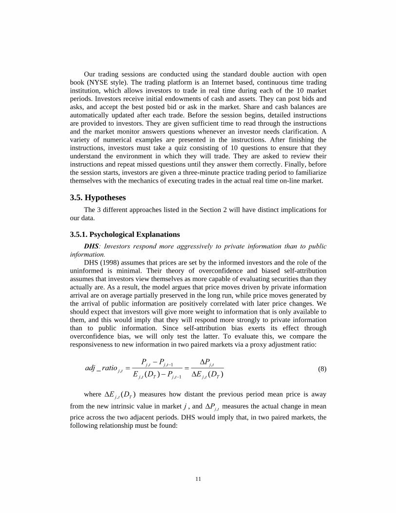
3.5.1. Psychological Explanations DHS: Investors respond more aggressively to private information than to public

information. DHS (1998) assumes that prices are set by the informed investors and the role of the

uninformed is minimal. Their theory of overconfidence and biased self-attribution assumes that investors view themselves as more capable of evaluating securities than they actually are. As a result, the model argues that price moves driven by private information arrival are on average partially preserved in the long run, while price moves generated by the arrival of public information are positively correlated with later price changes. We should expect that investors will give more weight to information that is only available to them, and this would imply that they will respond more strongly to private information than to public information. Since self-attribution bias exerts its effect through overconfidence bias, we will only test the latter. To evaluate this, we compare the responsiveness to new information in two paired markets via a proxy adjustment ratio:

)()(

_,

,

1,,

1,,,

Ttj

tj

tjTtj

tjtjtj DE

PPDE

PPratioadj

Δ

Δ=

−

−=

−

− (8)

where measures how distant the previous period mean price is away

from the new intrinsic value in market

)(, Ttj DEΔ

j , and tjP ,Δ measures the actual change in mean price across the two adjacent periods. DHS would imply that, in two paired markets, the following relationship must be found:

11

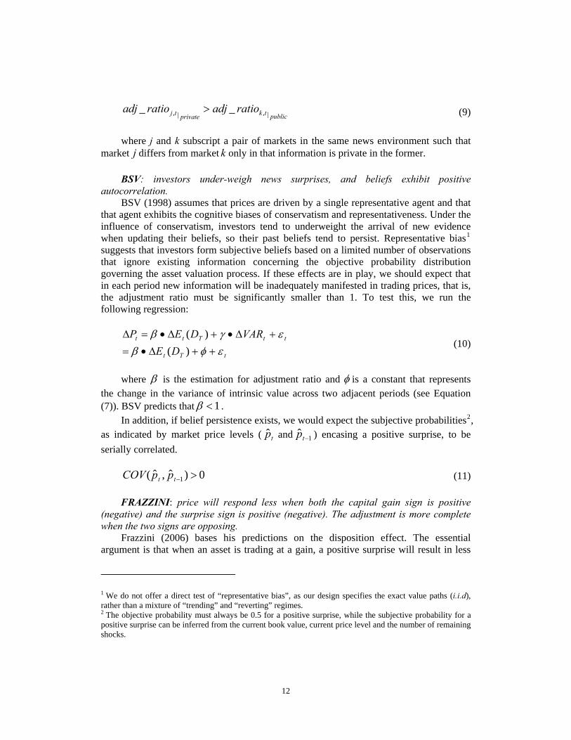
publictkprivatetj ratioadjratioadj|,|, __ > (9)

where j and k subscript a pair of markets in the same news environment such that

market j differs from market only in that information is private in the former. k BSV: investors under-weigh news surprises, and beliefs exhibit positive

autocorrelation. BSV (1998) assumes that prices are driven by a single representative agent and that

that agent exhibits the cognitive biases of conservatism and representativeness. Under the influence of conservatism, investors tend to underweight the arrival of new evidence when updating their beliefs, so their past beliefs tend to persist. Representative bias1 suggests that investors form subjective beliefs based on a limited number of observations that ignore existing information concerning the objective probability distribution governing the asset valuation process. If these effects are in play, we should expect that in each period new information will be inadequately manifested in trading prices, that is, the adjustment ratio must be significantly smaller than 1. To test this, we run the following regression:

tTt

ttTtt

DEVARDEP

εφβεγβ

++Δ•=+Δ•+Δ•=Δ

)()(

(10)

where β is the estimation for adjustment ratio and φ is a constant that represents

the change in the variance of intrinsic value across two adjacent periods (see Equation (7)). BSV predicts that 1<β .

In addition, if belief persistence exists, we would expect the subjective probabilities2, as indicated by market price levels ( and ) encasing a positive surprise, to be serially correlated.

tp̂ 1ˆ −tp

0)ˆ,ˆ( 1 >−tt ppCOV (11)

FRAZZINI: price will respond less when both the capital gain sign is positive

(negative) and the surprise sign is positive (negative). The adjustment is more complete when the two signs are opposing.

Frazzini (2006) bases his predictions on the disposition effect. The essential argument is that when an asset is trading at a gain, a positive surprise will result in less

                                                            

1 We do not offer a direct test of “representative bias”, as our design specifies the exact value paths (i.i.d), rather than a mixture of “trending” and “reverting” regimes. 2 The objective probability must always be 0.5 for a positive surprise, while the subjective probability for a positive surprise can be inferred from the current book value, current price level and the number of remaining shocks.

12

adjustment than a negative surprise because investors will rush to sell to lock in paper gains; and similarly, when asset is trading at a loss, a negative surprise will result in less adjustment than a positive surprise because investors will hold onto the asset and refuse to sell absent a premium. Thus Frazzini (2006) summarizes that when the signs are opposing the adjustment is complete, either because investors trading at a loss would be willing to accept the latest gain, or because investors trading at a gain would be willing to accept the latest loss. In our sessions, measuring the capital gain or loss is a simple task. According to Frazzini we would expect to observe that price adjustments following surprises would be less complete when the information content and the capital gain overhang have the same sign:

0,0, |_|_ <•>• Δ<Δ

tttt igtkigtj ratioadjratioadj (12) where is the proxy for capital gains and is the news surprise at period t . tg ti

3.5.2. Heterogeneous Investors HS: Pricing difference across two comparable periods in paired treatments can be

attributed to information asymmetry. HS (1999) posit that under-reacting anomalies may be generated when information

travels slowly. If information were scattered asymmetrically across different investors, those who rely on information accuracy for decision making would only act based on the information they are personally privy to; consequently, the process of information aggregation would fail. In the HS model of information aggregation failure, the market price equals to the weighted average of information implied values, discounted by the level of risk each group faces. In the private (asymmetric) information treatment, j, that price would be:

])([])([ 2111, tTtT

privatetj VARDEwVARDEwP •−+•−= θθ (13)

where ])([ 11 VARDE T •−θ is the valuation of the uninformed group,

])([ tTt VARDE •−θ is the valuation of the informed group, and and are the weights for each group. Because the uninformed group is completely blocked from information updating for the entire time span of the trading horizon and they fail to infer from market price, their valuation in every period would be the same as their valuation in period 1; for the informed group, their valuation would be updated whenever new information arrives. Similar to the assumptions in the HS model, the agents would act as a representative agent and the risk preference parameter,

1w 2w

θ , is assumed to be homogenous. In the public information treatment k, each investor is equally informed, therefore,

the equilibrium price is:

13

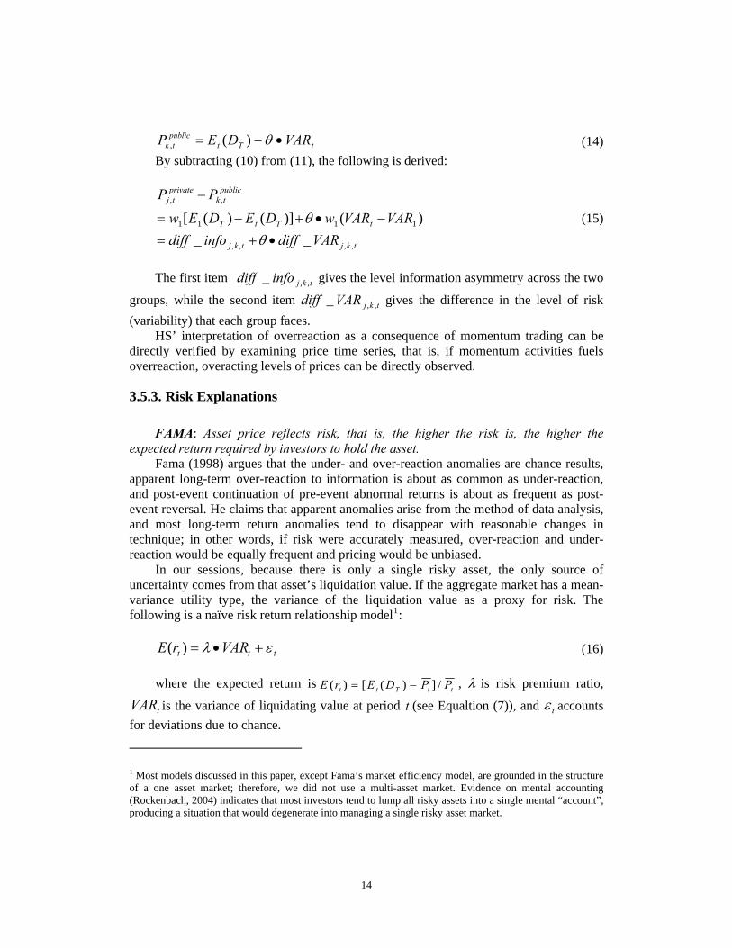
tTtpublictk VARDEP •−= θ)(, (14)

By subtracting (10) from (11), the following is derived:

tkjtkj

tTtT

publictk

privatetj

VARdiffinfodiffVARVARwDEDEw

PP

,,,,

1111

,,

__)()]()([

•+=−•+−=

−

θθ (15)

The first item gives the level information asymmetry across the two

groups, while the second item gives the difference in the level of risk (variability) that each group faces.

tkjinfodiff ,,_

tkjVARdiff ,,_

HS’ interpretation of overreaction as a consequence of momentum trading can be directly verified by examining price time series, that is, if momentum activities fuels overreaction, overacting levels of prices can be directly observed.

3.5.3. Risk Explanations FAMA: Asset price reflects risk, that is, the higher the risk is, the higher the

expected return required by investors to hold the asset. Fama (1998) argues that the under- and over-reaction anomalies are chance results,

apparent long-term over-reaction to information is about as common as under-reaction, and post-event continuation of pre-event abnormal returns is about as frequent as post-event reversal. He claims that apparent anomalies arise from the method of data analysis, and most long-term return anomalies tend to disappear with reasonable changes in technique; in other words, if risk were accurately measured, over-reaction and under-reaction would be equally frequent and pricing would be unbiased.

In our sessions, because there is only a single risky asset, the only source of uncertainty comes from that asset’s liquidation value. If the aggregate market has a mean-variance utility type, the variance of the liquidation value as a proxy for risk. The following is a naïve risk return relationship model1:

ttt VARrE ελ +•=)( (16)

where the expected return is ttTtt PPDErE /])([)( −= , λ is risk premium ratio,

is the variance of liquidating value at period t (see Equaltion (7)), and tVAR tε accounts for deviations due to chance.

                                                            

1 Most models discussed in this paper, except Fama’s market efficiency model, are grounded in the structure of a one asset market; therefore, we did not use a multi-asset market. Evidence on mental accounting (Rockenbach, 2004) indicates that most investors tend to lump all risky assets into a single mental “account”, producing a situation that would degenerate into managing a single risky asset market.

14

4. Experimental Results

4.1. Transaction Price Time Series and Drift The transaction prices of various market sessions evolve toward the intrinsic value

in diverse manners. We observe all sorts of patterns including upward momentum, downward momentum, U-shaped and humped-shaped time series. Incidences where transaction prices occur outside the range of possible intrinsic values are rare. The time series of transaction prices in all 24 market sessions are shown in Figure 2.

In the bearish environment, as shown in Panel 1-A (Session 3, 6, 13, and 16) and Panel 2-A (Session 5, 10, 15, and 22), prices converge to intrinsic value from above. In the neutral environment, as shown in Panel 1-B (Session 1, 11, 17, and 19) and Panel 2-B (Session 4, 9, 21, and 23) in Figure 2, the transactions start slightly below intrinsic value and quickly track it in later periods. In the bullish environment, as in Panel 1-C (Session 2, 8, 4, and 20) and Panel 2-C (Session 7, 12, 16, and 24), prices converge to intrinsic value from below. Under standard von-Neumann-Morgenstern utilities, agents price a symmetric payoff distribution below its expected value if they are risk averse, and price a symmetric payoff distribution above its expected value if they are risk seeking. However, we observe an inconsistency in that agents seem to be risk averse in pricing in the bullish environment and risk seeking in pricing in the bearish environment, even though the level of risk (variance of the intrinsic value) is the same for a particular period across all environments. The long-dash curve in Figure 2 is the Lowess 1 fitted line of the transaction prices, a computational method developed to assess scatter plots by robust locally weighted fitting. As shown in Figure 2, in the bearish and bullish environment, the market prices show clear patterns of downward and upward drift respectively. If we define under-reaction as the continuation of return signs, both cases strongly demonstrate this type of under-reaction drift. Under the neutral environment, the patterns are mixed but with smaller average deviations; most price trends are relatively flat, while some show a slight upward drift and some have a hump-shaped curve.

The 12 sessions on the left side of Figure 2 are sessions where information updates are publicly announced, while the 12 sessions on the right side are sessions where information updates are privately revealed to a subset of investors. The drifting patterns are similar across the two information conditions. (We will discuss this matter in more detail below.)

4.2. The Prevalence of Under-reaction The Lowess fitted curves offer an intuitive representation of under-reaction patterns

in which returns hold the same sign from the news release at the session opening to the liquidating point.

                                                            

1 Lowess was introduced in “Visual and Computational Considerations in Smoothing Scatter plots by Locally Weighted Fitting,” W. S. Cleveland, Computer Science and Statistics: Eleventh Annual Symposium on the Interface, North Carolina State University, Raleigh, North Carolina, 1978, pages 96-100.

15

Laboratory studies provide the advantage of being able to directly assess both the signs and the magnitudes of reaction, rather than having to solely rely on prices to infer deviations from intrinsic value. The average deviations of transaction prices from intrinsic value in every trading period across all market sessions are plotted in Figure 3. Deviations are essentially equivalent to expected returns.

As shown in Figure 3, in the bearish environment we observe large overpricing (negative expected returns) relative to the intrinsic value in almost all markets, with higher deviations in initial periods. In the bullish environment, we observe large under-pricing (positive expected returns) relative to the intrinsic value in 7 out of 8 sessions, with all sessions being more severely underpriced initially. In the neutral environment, a roughly even split is found between under-pricing and overpricing. The drifting patterns in bullish and bearish sessions epitomize the definition of under-reaction, while the neutral sessions appear to show return reversals in numerous cases even as they flatten out on average.

To construct a better classification rule of sorting underreation and overreaction for each period, we consider evaluate the temporal position of transaction prices relative to intrinsic values. Below we define under-reaction using a price migration rule with both a short and long-term lens.

The long-term identification is judged by the price position relative to the intrinsic value over the session’s entire duration. In all sessions, before beginning all investors are informed about the (approximately normal) distribution of the asset liquidation value. Suppose the prices start on one side of this intrinsic value, move away from past price (average price in all past periods) and migrate to the other side of the intrinsic value, then the pricing of the trading period is interpreted as over-reaction; if the prices keep proximate to past price and always fall short of reaching the intrinsic value, the pricing of a trading period is interpreted as under-reaction. (See the left panel in Figure 4.)

We precisely define the short-term reaction for each trading period such that the price migration is examined within the two-period time window enveloping an information event (See right panel in Figure 4):

⎪⎩

⎪⎨⎧

<−

>−=

−−

−−

)(),(

)(,)(_

11

11

TttTtt

TtttTt

DEPifDEP

DEPifPDEmagnitudeshort (17)

where 1−tP is the average transaction price in period t-1 and the sign of the deviation

is dependent upon the position of price relative to intrinsic value in the previous period. We precisely define the long-term reaction magnitude in the same fashion except

that the price migration is examined across all transpired periods:

⎪⎩

⎪⎨⎧

<−

>−=

−−

−−

)(),(

)(,)(_

1...11...1

1...11...1

TttTtt

TtttTt

DEPifDEP

DEPifPDEmagnitudelong (18)

16

where tP is the average transaction price in the current period , t 1...1 −tP is the average transaction price over all previous periods, is the intrinsic value as of

period t ,

)( Tt DE)(1...1 Tt DE − is the average intrinsic value over all previous periods; and the sign

of the deviation is dependent upon the position of average past price relative to average past intrinsic value.

In both cases, if the reaction magnitude is negative, the pricing will be interpreted as under-reaction, and if the reaction magnitude is positive, the pricing will be interpreted as over-reaction.

⎩⎨⎧

>−<−

=0,

0,_

magnitudeifreactionovermagnitudeifreactionunder

typereaction (19)

The distribution of reaction magnitude is shown in Figure 5. Among 238 trading

periods in 24 sessions, in the long run, 71.8% of the periods have current trading prices staying on the same side of intrinsic value as previous average price, while 28.2% of the periods display migration to the other side of intrinsic value. In the short run, 82.8% of the periods have current trading prices staying on the same side of intrinsic value as the previous period price, while 17.2% of the periods display migration to the other side. We note that both distributions are left skewed with a mean less than zero, indicating that under-reactions dominate not only in frequency but in magnitude too. This confirms the empirical findings suggesting dominance of under-reaction in the short run, and also rejects Fama’s (1998) claim that under-reaction and over-reaction cancel out on average in the long run.

In addition, we evaluate our methodology against the traditional return sign characterizations. We measure return as the price percentage change across two adjacent periods, and classify the periods where pre-event-period return and post-event-period return have the same signs as “under-reaction”, and opposing signs as “over-reaction”. We found 113 periods of “under-reaction” and 80 periods of “over-reaction”. For the long term return, we classify the periods where pre-event cumulative return1 and post-event return have the same signs as “under-reaction”, and opposing signs as “over-reaction”. We found 93 periods of “under-reaction” and 83 periods of “over-reaction”.

However, an implicit assumption is made that the continuation of return signs indicates inadequate past adjustment, while the reversal of return signs indicates excessive past adjustment. The problem lies in that we generally do not have the knowledge of whether: (a) the magnitude of the previous adjustment is sufficient or excessive; (b) the previous price is converging to or diverging from the intrinsic value. A glimpse at the time series paths shown above suggests that these worries are not superfluous. For instance, in Session 21, the turning in return sign at period 5 is an

                                                            

1 Fama (1998) argues that long-term return should be computed by average abnormal return (AAR) or cumulative abnormal return (CAR) as buy-and-hold return (BAHR) tends to have higher errors. We use CAR in our analysis.

17

accurate reflection of the turn in the intrinsic value; and in Session 4, the continuation of return around period 5 is actually a movement away from intrinsic value.

Pure return-sign based classification is problematic because a change in return sign is not necessarily the result of previous excessive adjustment and a stationary return sign is not necessarily the result of previous inadequate adjustment; rather, the behavior of a post event return can simply be a correct adjustment to the new status quo.

4.3 Sources of Overreaction The plots in the neutral environment in Figure 3 hint an important potential cause for

over-reaction. Most over-reactions appear in the neutral environment, yet Panel 1-B and 2-B in Figure 2 show that it is the change in the intrinsic value rather than the change in the price that generates the patterns.

The migration of price from one side of intrinsic value to the other side is considered as overreaction; however, the migration can be either caused by the excessive adjustment in price or the change in the intrinsic value coupled with sluggish price adjustment. We conduct analysis on 41 periods of overreaction out of a total of 238 periods. Table III tabulates all the overreaction periods into four scenarios: (a) price migrates from below to above and the news surprise is positive; (b) price migrates from below to above and the news surprise is negative; (c) price migrates from above to below and the news surprise is positive; d) price migrates from above to below and the news surprise is negative. Case (a) and (c) indicate that the price adjustment not only corrects the previous period deviation but also absorb fully the news surprise, therefore, both cases relates to excessive adjustment version of overreaction. Case (b) and (d) indicates that the price adjustment is insufficient such that it does not absorb fully the news surprise, therefore, both cases relates to insufficient adjustment.

The results in Table III suggest that overreaction (migration to the other side of intrinsic value) is mostly generated by sluggish adjustment (34 periods), rather than excessive adjustment (only 7 periods).

Indeed, we will examine the overall magnitude of the sluggish adjustment in Section 5.1.2; indeed, we will show that sluggish adjustment prevails in our data and the average adjustment to news surprise is only 38%. (Refer to Table V)

5. Verifying the Competing Models Section 4 has demonstrated the dominance of under-reaction phenomenon across all

sessions, especially under the bullish and bearish environments. In this Section, we will evaluate more specifically the unique predictions of the five competing models.

18

5.1. Psychological Explanations

5.1.1. DHS DHS (1998) predicts that agents will respond more actively to privately held

information. That means that when information updates reach only an insider group, due to overconfidence those insiders will trade more aggressively and lead the market to over-reaction.

As specified in the hypotheses, DHS has straightforward implications for the rate of adjustment. We derive the difference in adjustment rate by pairing the adjustment rate in a particular period of the private information treatment with the same period of the public information treatment:

publictjprivatetjtkj ratioadjratioadjratediff |,|,,, ___ −= (20)

DHS suggests that the term should be strictly positive while HS suggests that it

should be strictly negative. Figure 6 provides the histogram for the paired difference in adjustment rates.

The histogram indicates that the distribution is hardly distinguishable from the zero mean symmetric normal distribution, and we cannot reject that hypothesis given the Student t test generates a p-value of 0.82.

Table IV lists the average turnover, bid-ask spread, mean price, median price and

closing price for all 24 sessions, using each trading period as an observation. Across the two information conditions, none of these measures differ substantially except volume. It is noteworthy that there is considerable reduction in volume when information is privately revealed. We note that the reduction is mostly derived from uninformed investors who involved in many fewer transactions than their counterparts in the public information treatment.

5.1.2. BSV Model BSV argues that once agents form beliefs they will become reluctant to change this

prior and will tend to under weigh the arrival of new information. In Figure 7, we graph the adjustment rate distribution and show it is leptokurtic and positively skewed. In 60.7% of the cases price adjusts in the correct direction but insufficiently, in 26.4% of the cases price adjusts in the opposite direction of the surprises, and in 12.9% of the cases price adjusts in excess of the intrinsic value change. Insufficient adjustment is the dominant phenomenon. Starting from the initial deviation from intrinsic value until eventual convergence, the sessions adjust average valuation hesitantly on the path to liquidation. As prices are the manifestation of agents’ beliefs, the inertia in prices can be understood as inertia in willingness to change beliefs.

Next, we run regressions on how swiftly prices on average adjust to intrinsic value changes. The regressions in Table V show that the average adjustment to surprises to intrinsic value is around 38%. The effect is robust using mean, median and closing prices,

19

and the coefficients are significant at 0.01 level. In addition, the dummy variable does not have a significant effect on the rate of adjustment. kprivate

The BSV model also implies that agents tend to ignore new information and exhibit belief persistence. To demonstrate the belief continuation argument of BSV model, we derive the session’s aggregate subjective probability estimates from observed prices. The natural probability for a Head draw is always 0.5. However, the subjective probability of agents in the sessions can hardly be the same as 0.5 because prices persistently deviate from intrinsic value. In every trading period, given the current level of price, we can derive the subjective probability (of a Head draw). This offers a perspective that allows us to probe the investors’ subjective beliefs1.

We denote a session’s aggregate belief on the probability of Head draw in period t as . Because current period price reflects the market’s average belief on the probability of a Head draw, the following equality should hold:

tp̂

])ˆ1(ˆ)[()( dpuptTDDEP tttTtt −−−+== (21)

tP is the average trading price in period . t Figure 8 shows the evolution of subjective probability across adjacent periods in the 24 sessions. Most points in the scatter plot reside in the 1st and 3rd quadrants, indicating that an underestimated subjective probability (negative deviation) in one period is likely to be followed by an underestimated subjective probability (negative deviation) in the next period, too. This is in accordance with BSV’s prediction of belief persistence.

5.1.3. Disposition Effect The disposition effect (Shefrin and Statman, 1985; O’dean, 1998; and Grinblatt and

Han, 2001) has been given much attention in recent empirical research. This theory predicts that investors will rush to sell after a capital gain and are

reluctant to sell after a capital loss. Frazzini (2006) proposes that the presence of ‘disposition’ investors will depress prices following good news as they rush to sell to lock in paper gains, and will halt prices from falling following bad news as they are reluctant to sell absent a premium. Table VI summarizes the predictions of Frazzini (2006).

The key variable for testing the disposition effect is the measure of capital gains. Similar to Frazzini (2006), we measure the reference price as the volume weighted historic average price:

                                                            

1 Measuring implied probability offers us a unified way to look at deviations across different sessions. It has an important advantage over measuring deviation directly. Because 1 unit of deviation in the first period tends to be less significant than 1 unit of deviation in the latest period, implied probability provides a convenient way of weighting deviations across periods.

20

∑

∑−

=

−

=

×= 1

1

1

1t

ii

t

iii

t

Volume

VolumePRP (22)

Then we compute capital gain overhang as:

t

tt

t

ttt P

RPPP

RPPg −=

−= (23)

The results in Table VII clearly reject Frazzini (2006). We observe more adjustment

in cases where news content and capital gains hold the same sign, contrary to the disposition effect prediction. In addition, the number of asks in the market seems to remain relatively unchanged across various gain conditions.

5.2. Heterogeneous Investors: HS Hong and Stein’s information diffusion model suggests that information aggregation

failure arising from information asymmetry will keep the market price away from full information implied values. As specified in Equation (9) in our hypotheses, the price in a given period of a private information session and in the same period of a public information session should reflect the information asymmetry and associated difference in uncertainty amongst investors. Note that for each pair of comparable periods, every factor is kept the same except for how many investors are told the content of surprises.

Table VIII runs regression analysis on Equation (9) and provide no support for the relationship between information asymmetry and price difference. That is, the average valuation of informed traders and uninformed traders does not capture the temporal development of prices. This result comes as no surprise, as Figure 2 shows that the price series in the two treatments are extremely alike.

We do not observe that continuation of trends leads price to migrate to the other side of intrinsic value. In most sessions, the markets spend the whole experiment session in converging to the intrinsic value. (See to Figure 3) It is clearly shown that under-reaction prevails while overreaction reversals happen mostly when the intrinsic value evolution changes its initial cause. Hence, there is no reasonable basis to assume over-reaction in our data is caused by a separate set of momentum traders.

5.3. Risk based Explanation: Fama Fama (1998) argues that on average over-reaction and under-reaction should cancel

out. The histograms in Figure 5 indicate that under-reaction dominates over-reaction both in magnitude and in frequency.

Empirical findings of anomalies can arise from imperfect evaluation of risk factors, but we can precisely measure the price deviations in our data against current intrinsic

21

value uncertainty. In our trading sessions there is only one source of uncertainty: the variance of the intrinsic value which is a linear function of the number of pending surprises. The risk associated with the intrinsic value uncertainty, as measured by its variance, declines over time. If agents are risk averse (seeking) in valuing the symmetric intrinsic value distribution, the required rate of return should be positive (negative) to entice trade.

We do not observe such consistency. Figure 9 shows that the aggregate risk-return compensation ratio (the long-dash line) is indistinguishable from zero. However, though investors are exposed to the same level of uncertainty in the same period in all the environments, they consistently require a premium to final claims in the bullish environment, a zero premium in the neutral environment, and strikingly, a discount in the bearish environment. The higher the risk, the more pronounced is this effect.

If the variance of intrinsic value is not a perfect proxy for risk, a weaker test would be that since for any given period t each unit held is exposed to the same surprise distribution, with the same level of variability, the compensations across different environments should, on average, be equal to each other.

( ) ( ) ( ) TtbearishrEneutralrEbullishrE ttt ,,2,1,||| L=== (24)

Table IX indicates that the compensations in each period are not equal across the

three news environments, but there exists a systematic difference. Under the bearish environment an average negative expected return of -15.7% is observed, while under the bullish environment an average positive expected return of 7.3% is observed. In neutral environment, the overall average expected return is 0. A stage-wise cross section comparison reveals this result even more convincingly, as the expected return is always largest for the bullish environment and smallest for the bearish environment. This substantively rejects Equation (20) and seriously questions whether under-reaction (over-reaction) can be explained by risk attitudes.

6. A Theory of Price Inertia: Numeric Simulations In Section 4.3, a tentative conclusion is reached that sluggish adjustment is

responsible for the emergence of overreaction. It remains unverified whether price inertia can be the sole driver of the relative frequencies of under- and over-reaction.

This Section will simulate, using parameters obtained from the data, to demonstrate the speed of adjustment is the key factor in generating under- and over-reaction. That is, when the market response to news surprise is sluggish, both regularities will emerge with the former outnumbering the latter; when the market response to news surprise is excessive, both regularities will again emerge but the latter outnumbering the former. The only input variable to be controlled is the speed of adjustment and we will analyze the results respectively.

22

6.1 Simulation Setup The analysis has indentified insufficient adjustment as a prevailing phenomenon

under all conditions. We now turn to a simulation experiment to examine how the speed of short-term adjustment might impact the under- and over-reaction patterns we observe.

The set-up of the simulation is exactly the same as laid out in the experiment design. To drive the simulation we derive two parameter values from the data: the starting price and the adjustment ratio. Our data imply that: and

.

)0.110,6.507(~ 21 NP

)81.0,27.0(~_ 2NratioadjThe purpose is to vary the distribution of adjustment ratio and evaluate how the

under- and over-reaction patterns change accordingly. We choose three alternate distributions for adjustment ratio: insufficient adjustment, ,

which was observed in our data, appropriate adjustment, , which might be observed if price adjustments were accurate on average, and excessive adjustment, , which might be observed if price adjustments were aggressive on average. In addition, we use both the short-term and long-term perspectives introduced earlier to analyze the reaction magnitudes.

)81.0,27.0(~_ 2Nratioadj)81.0,1(~_ 2Nratioadj

)81.0,73.1(~_ 2Nratioadj

6.2 Simulation Results and Discussion The simulation results suggest that the adjustment ratio is the key factor driving the

reaction distributions. When the average adjustment ratio is below 1, under-reaction dominates (Figure 10, Panel A-1 and B-1); when the average adjustment ratio is 1, under-reaction is as frequent as over-reaction (Figure 10, Panel A-2 and B-2); when the average adjustment ratio is greater than 1, over-reaction dominates (Figure 10, Panel A-3 and B-3). These results hold for both short and long-term perspective (See Table X). There is a slight tendency for over-reaction to grow when switching to long-term perspective, which is consistent with empirical results that over-reaction tend to show up more in the long term.

The simulation reveals an important message: over-reaction and under-reaction are both by-products of the adjustment responsiveness in the environment. Overreaction is also created by inertia because the price adjustment does not catch up with the speed of change in the intrinsic value. Whether the pricing at a point should be classified as under- or over-reaction largely depends on the past, whereas the point-of-time prices in the two labeling situations could have been exactly the same. Note that at any point of time, price is slowly correcting its error. In our sessions, they simultaneously derive in the proportions observed from the same cause: slow adjustment.

7. Conclusion How market prices incorporate the arrival of new information has long been a puzzle

to theorists and empirical researchers. In this paper, we designed and collected data from controlled laboratory markets that replicate a version of the HS (1999) information

23

diffusion model. We structured the information arrivals such that they were temporally dispersed and asymmetrically held across individual investors. The multi-period exchange economy allowed us to evaluate observed price dynamics against the predictions of various competing models.

The trading price time series data manifests under-reacting drifts in both bullish and bearish environments. The bullish environment was usually interpreted by investors as not as good enough (under-pricing persisted), while the bearish environment was interpreted as not bad enough (over-pricing persisted). This gives the impression that agents are risk seeking in bearish environments and risk averse in bullish environments, even though at each period, we designed the risk exposure to be identical across these environments. We found the risk-return premium relationship does not hold in attributing abnormal returns to chance.

Information asymmetry had no significant affect on price adjustments, both over the short and long terms. The level of information asymmetry did not explain the price difference across two comparable trading periods. This questions the HS’ arguments that the failure of information aggregation may be a reason for under-reaction and that asymmetric information slows down the adjustment process toward intrinsic value. The DHS overconfidence model predictions are not confirmed in our private information treatment, as privately informed investors were not found to lead the markets to over-reaction. Furthermore, capital gains and losses did not correlate with price adjustment magnitude in the fashion specified by the disposition effect model.

An analysis of the sessions’ subjective probabilities indicated that biased judgments tend to persist and exhibit belief continuation. The inertia patterns discovered were most consistent with the conservatism account of BSV among existing theories.

We identified both the short-run and long-run under and over-reaction distributions with the advantage of knowing perfectly the intrinsic asset values. Under-reaction is the predominant regularity in all markets in the short run, while under-reaction dominates the long term price behavior in both bullish and bearish environments, but dissipates in the neutral environment. We showed that the common technique of return sign characterization with ignorance of intrinsic value or accurate estimation techniques can produce misleading conclusions. Over-reacting types of price adjustments were not necessarily the markets’ excessive adjustment to earlier information. That is, the initial adjustment might be appropriate, while later stage price reversals were the market’s re-adjustment to a new intrinsic value, with inertia generating a prolonged period of opposite return signs.

Sizable over-reaction is present in the clearly under-reaction predominated markets as well. This leads us to hypothesize: are under-reaction and over-reaction caused by the same matter? A re-examination of our results and a simulation with the parameters extracted from data suggest that consciously conservative adjustments alone provide an account for both under- and over-reaction regularities. The empirical and theoretical dichotomy of treating the two anomalies might be questionable. Our simulation suggests that simple inertia is the key factor in determining the distribution of reaction magnitudes, and that slow adjustment is the reason for both under- and over-reaction regularities observed.

24

No single theory presented in this paper can totally summarize the informational efficiency shown in the data. Investors exhibited belief continuation and accordingly prices displayed inertia. Investors seemed to place considerable weight on their previous beliefs (past price) when forming valuations about uncertain future payoffs. Both short-run return continuations (driven by slow adjustment) and long-run return reversals (possibly re-adjustments to evolutionary turns in intrinsic value) can be explained by price inertia (belief continuation).

25

Appendix

Appendix A: Asset with a random walk intrinsic value and information diffusion

Hong and Stein (1999) define an asset which pays a single dividend at the liquidating date.

This liquidating dividend is ∑ =+=

T

j jT DD10 ε . At each period , investors trade claims on

the risky asset. The asset pays a single liquidating dividend at time

t

T . ε ’s are the dividend innovations and are assumed i.i.d, normal random variables

. ),0(N~ 2σε

To incorporate the notion that information moves gradually across the "newswatcher population", they divide this population into z equal-sized groups and every dividend innovation, jε , can be decomposed into z independent sub-innovations ij ,ε ,

with zjjjij ,2,1,, εεεε ++= L , each with variance . z/2ε

The timing of information release is as follows: at t, news about ε t+z−1, begins to spread, and newswatcher group 1 observes εt+z −1, 1, group 2 observes εt+z −1,2 , . . ., group z observes εt + z − 1, z. At t, each sub-innovation of εt+z −1, has been seen by a fraction 1/z of the total population. At t+1, the groups “rotate”, group 1 now observes εt+z−1, 2, group 2 observes εt+z−1, 3, . . ., group z observes εt + z − 1, 1. At t+1 the information εt+z −1 has spread further, and each sub-innovation of εt+z −1, has been seen by a fraction 2/z of the total population. Rotation continues until time t + z − 1, at which point every one of the z groups has directly observed each of the sub-innovations that comprise εt +

z − 1. εt + z − 1, has become totally public by time t + z − 1.

The parameter z can be thought of as a proxy for the rate of information flow. Higher values of z imply slower information diffusion1.

The model predicts that because newswatchers fail to infer intrinsic value from market prices, they rely on their private information in deciding their demand and consequently, under-reaction is more severe when information diffuses more slowly. Note that, though the authors claim the diffusion primarily occurs through dissemination across the population, it is in fact mixed cross-population and over-time diffusion. The reason is simple: the faster that traders to get know future dividend innovations, the earlier they learn about their future situations. The price at time t should equal to:

QzzzDP zttttt •−++−+−+= −+++ θεεε /]...)2()1[( 121

                                                            

1 Higher z, on the one hand, means more numbers of traders; and on the other hand, it means the diffusion of information for a longer time horizon. Therefore, higher z not only indicates slower diffusion across the investor public, but also more fundamental uncertainty that spans over time.

26

where θ is a function of newswatchers’ risk aversion and the variance of theε ’s.

Glosten (1985) posits the opposite, that is, the price at time t should equal to:

QDP ztt •−= −+ θ1

Nonetheless, the authors argue that investors will fail to infer intrinsic value from prices and such equilibrium will be impossible.

HS has two essential features. First, as time passes and more value innovations are realized the uncertainty of the liquidating dividend declines. Second, there is information asymmetry among the investor public, with some investors holding a more accurate estimate of the intrinsic value. The first feature is readily feasible in the laboratory as long as we keep the time horizon finite. The second feature, asymmetry, is more difficult to implement in the laboratory exactly as specified by Hong and Stein (1999), because rotation is an awkward scenario and rotating information concerning sub-innovations are not an intuitive concept to explain to investors.

To make the scenario readily digestible for investors, we keep the first HS feature, delete the sub-innovation feature, and simplify the asymmetry among investor public by having a fixed group of investors that receive private information during the trading periods. As a design control this private information treatment is paralleled with a public information treatment where all investors are equally informed simultaneously. This simplification enables us to implement the laboratory trading sessions with much less cognitive cost on the part of investors and a much more intuitive explanation for the privileged few, while retaining the essential information diffusion both across time and the population.

Appendix B: Data Data is available at http://esi2.chapman.edu/sandler/24mkt.txt Data dictionary is provided below: Info: 0="public", 1="private" Environment: -1="bad"; 0="neutral"; 1="good" Action 1="buy", 2="sell", 3="bid", 4="ask", 5="cancel buy", 6="cancel sell"

Appendix C: Experiment Instructions Public Information, Bullish Environment: http://esi2.chapman.edu/sandler/rw_inc/page1.html Public Information, Neutral Environment: http://esi2.chapman.edu/sandler/rw_con/page1.html Public Information, Bearish Environment: http://esi2.chapman.edu/sandler/rw_des/page1.html Private Information, Bullish Environment, Informed Group:

27

http://esi2.chapman.edu/sandler/private/rw_inc/page1.html Private Information, Bullish Environment, Uninformed Group: http://esi2.chapman.edu/sandler/dark/rw_inc/page1.html Private Information, Neutral Environment, Informed Group: http://esi2.chapman.edu/sandler/private/rw_con/page1.html Private Information, Neutral Environment, Uninformed Group: http://esi2.chapman.edu/sandler/dark/rw_con/page1.html Private Information, Bearish Environment, Informed Group: http://esi2.chapman.edu/sandler/private/rw_des/page1.html Private Information, Bearish Environment, Uninformed Group: http://esi2.chapman.edu/sandler/dark/rw_des/page1.html

28

References: Abarbanell, Jeffery S., and Reuven Lehavy, 2003, Role of reported earnings in explaining

apparent bias and over/under-reaction in analysts' earnings forecasts, Journal of Accounting and Economics 36, 105–146.

Barberis, Nicholas C., Andrei Shleifer, and Robert W.Vishny, 1998, A model of investor sentiment, Journal of Financial Economics 49, 307-343.

Bernard, Victor L., and Jacob K. Thomas, 1989, Post-earnings-announcement drift: Delayed price response or risk premium? Journal of Accounting Research 27, 1-33.

Gunduz, Caginalp, David P. Porter, and Vernon L. Smith, 2001, Financial bubbles: Excess cash, momentum, and incomplete information, Journal of Psychology and Financial Markets 2(2), 80-99.

Daniel, Kent D., David A. Hirshleifer and Avanidhar Subrahmanyam. 1998, A theory of overconfidence, self-attribution, and security market under- and over-reactions, Journal of Finance 53, 1839–1886.

DeBondt, Werner F.M., and Richard H. Thaler, 1985, Does the stock market overreact? Journal of Finance 40, 793-805.

DeBondt, Werner F.M., and Richard H. Thaler, 1987, Further evidence on investor over-reaction and stock market seasonality, Journal of Finance 42, 557-581.

DeBondt, Werner F.M., and Richard H. Thaler, 1990, Do security analysts overreact? American Economic Review 80(2), 52-57.

Dreman, David N. and Eric A. Lufkin, 2000, Investor over-reaction: Evidence that its basis is psychological, The Journal of Psychology and Financial Markets 1(1), 61-75.

Edwards, Ward, 1968. Conservatism in human information processing. In: Kleinmutz, B. (Ed.), Formal Representation of Human Judgment. Wiley, New York.

Fama, Eugene F, 1998, Market efficiency, long-term returns and behavioral finance, Journal of Financial Economics 49, 283-306.

Fama, Eugene F, 1970, Efficient capital markets: A review of theory and empirical work, Journal of Finance 25, 383-417

Frazzini, Andrea, 2006, The disposition effect and under-reaction to news, Journal of Finance 62, 2017-2046.

Grinblatt, Mark, and Bin Han, 2005, Prospect theory, mental accounting, and momentum, Journal of Financial Economics 78, 311-339.

Glosten, Lawrence R. and Paul R. Milgrom, 1985, Bid, ask and transaction prices in a specialist market with heterogeneously informed traders, Journal of Financial Economics 14, 71–100.

Grossman, S. 1976, On the efficiency of competitive stock markets where traders have diverse information, Journal of Finance 31, 573-85.

Hong, Harrison, and Jeremy C. Stein, 1999. A Unified Theory of Under-reaction, Momentum Trading and Over-reaction in Asset Markets. Journal of Finance, 54, 2143–2184.

Hong, Harrison, Terrence Lim, and Jeremy C. Stein. 2000, bad news travels slowly: Size, analyst coverage, and the profitability of momentum strategies, Journal of Finance 55, 265–295.

Ikenberry, David L., Josef Lakonishok, and Theo Vermaelen, 1995, Market under-reaction to open market share repurchases, Journal of Financial Economics 39, 181-208.

Ikenberry, David L., and Sundaresh Ramnath, 2001, Under-reaction to self-selected news events: The case of stock splits, Review of Financial Studies 15, 489-526.

Jegadeesh, Narasimhan, and Sheridan Titman,1993, Returns to buying winners and selling losers: Implications for stock market efficiency, Journal of Finance 48, 65–91.

29

Mikhail, Michael B., Beverly R. Walther, and Richard H. Willis, 2001, The effect of experience on security analyst under-reaction and post-earnings-announcement drift, Journal of Accounting and Economics 35, 101-116.

O'dean, Terrance. 1998, Are investors reluctant to realize their losses? Journal of Finance 53 (5), 1775-1798.

Rockenbach, Bettina, 2004, The behavioral relevance of mental accounting for the pricing of financial options, Journal of Economic Behavior and Organization 53, 513-527.

Shefrin, Hersh M., and Meir Statman, 1985, The disposition to sell winners too early and ride losers too long: Theory and evidence, Journal of Finance 40, 777-790.

Smith, Vernon L. 1982, Microeconomic systems as an experimental science, American Economic Review72 (5), 923-955.

30

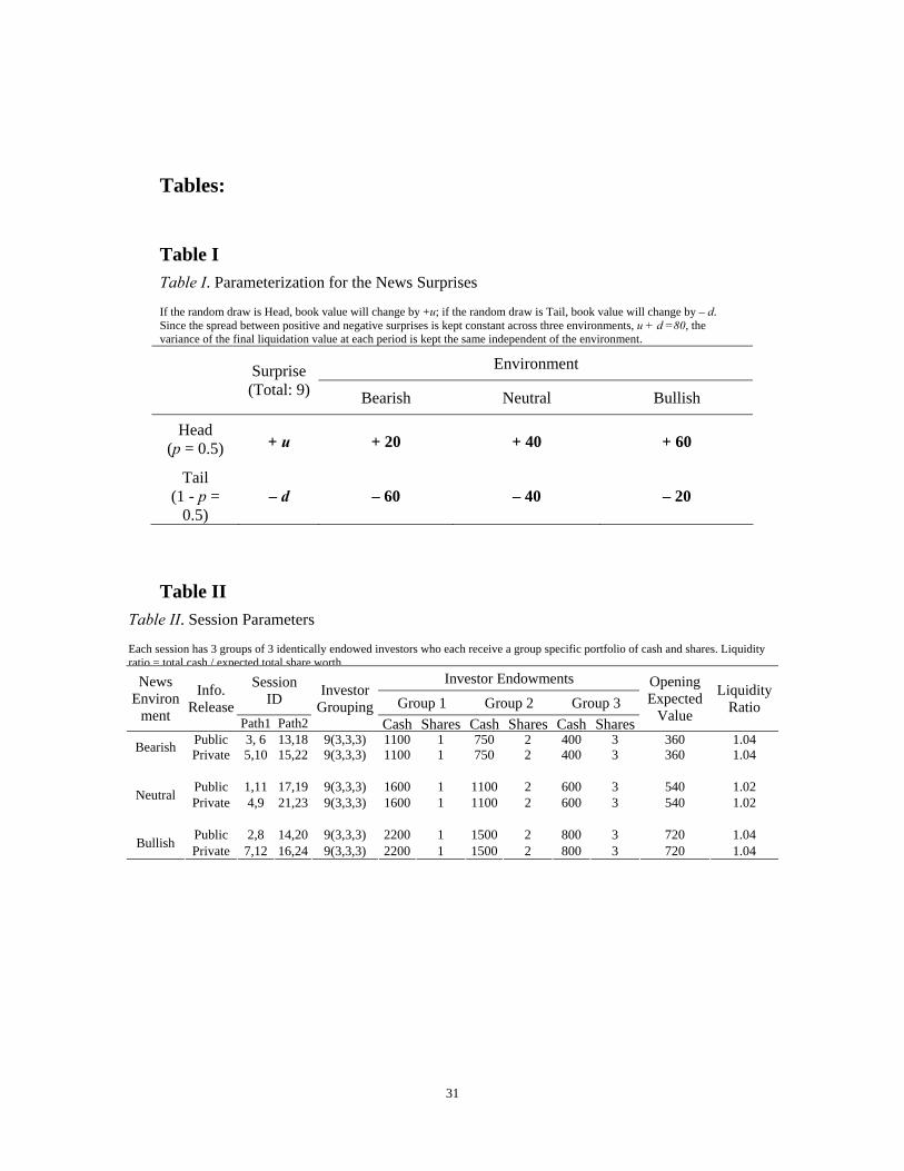
Tables:

Table I Table I. Parameterization for the News Surprises If the random draw is Head, book value will change by +u; if the random draw is Tail, book value will change by – d. Since the spread between positive and negative surprises is kept constant across three environments, u + d =80, the variance of the final liquidation value at each period is kept the same independent of the environment.

Environment Surprise (Total: 9) Bearish Neutral Bullish

Head (p = 0.5)

+ u + 20 + 40 + 60

Tail (1 - p =

0.5) – d – 60 – 40 – 20

Table II Table II. Session Parameters Each session has 3 groups of 3 identically endowed investors who each receive a group specific portfolio of cash and shares. Liquidity ratio = total cash / expected total share worth.

Investor Endowments Session ID Group 1 Group 2 Group 3

News Environ

ment

Info. Release

Path1 Path2

Investor Grouping

Cash Shares Cash Shares Cash Shares

Opening Expected

Value

Liquidity Ratio

Public 3, 6 13,18 9(3,3,3) 1100 1 750 2 400 3 360 1.04 Bearish Private 5,10 15,22 9(3,3,3) 1100 1 750 2 400 3 360 1.04

Public 1,11 17,19 9(3,3,3) 1600 1 1100 2 600 3 540 1.02 Neutral Private 4,9 21,23 9(3,3,3) 1600 1 1100 2 600 3 540 1.02

Public 2,8 14,20 9(3,3,3) 2200 1 1500 2 800 3 720 1.04 Bullish Private 7,12 16,24 9(3,3,3) 2200 1 1500 2 800 3 720 1.04

31

Table III Table III. Sources of Overreaction: Insufficient adjustment v.s. excessive adjustment

Overreaction is classified when price migrates to the other side of intrinsic value across two adjacent periods. 41 of 238 periods are classified as overreaction periods in the data. In 34 out of the 41 overreaction periods, prices do not catch up with the new intrinsic value and thus migrate to the other side; in 7 out of the 41 overreaction periods, prices adjustment excessively and migrate to the other side.

Deviation from Intrinsic Value Surprise in Current Period

Previous Period Current Period + –

– + 4 18 + – 16 3

 

Table IV Table IV. Comparison on Other Measures across Information Condition

The numbers in parenthesis are standard deviations. Each pair consists of the measures in a period of the private information sessions and the counterpart in the public information sessions. All other conditions remain the same except for the information privacy. The student t test hypothesizes that the paired difference holds a mean of zero.

Public Private Student t Paired Comparison p-value

Volume 12.9 (10.7)

8.4 (9.7) p=0.049**

Bid-Ask Spread 188.9 (129.3)

221.6 (158.9) p=0.08

Mean Price 542.7 (111.8)

538.7 (116.2) p=0.787

Median Price 543.5 (112.2)

540.6 (116.6) p=0.84

Closing Price 550.2 (121.5)

544.4 (123.4) p=0.718

32

Table V Table V. Feasible GLS Regressions on Adjustment Rate The number in parenthesis is the z-statistic. *** stands for 0.01 significance level, and ** stands for 0.05 significance level. The coefficients are estimated with generalized least squares, with heteroskedasticity and panel-specific AR(1) autocorrelation. ΔPk,t represents the change in price in session k from period t-1 to period t. ΔEk,t(DT) represents the difference between current intrinsic value and past period average (median or closing) price.

Panel A: Descriptive Statistics N Mean Std. Dev. Min Max

mean 212 4.4 40.3 -117.0 164.5 median 212 5.0 43.0 -116.0 185.0 ΔPk,t closing 212 1.6 64.4 -235.0 290.0

ΔEk,t(DT) 216 1.2 76.1 -179.4 227.8

Panel B: Regression Results ΔPk,t Independent Variable mean median closing

ΔEk,t(DT) 0.38 (8.48***) 0.34 (7.12***) 0.42 (5.13***) privatek 1.78 (0.39) 0.54 (0.11) 2.66 (0.33) environmentk(=neutral) 17.15 (3.08***) 17.06 (2.78***) 7.74 (0.77) environmentk(=bullish) 28.79 (5.17***) 29.00 (4.72***) 25.87 (2.57**) constant -22.24 -25.25 -18.21

33

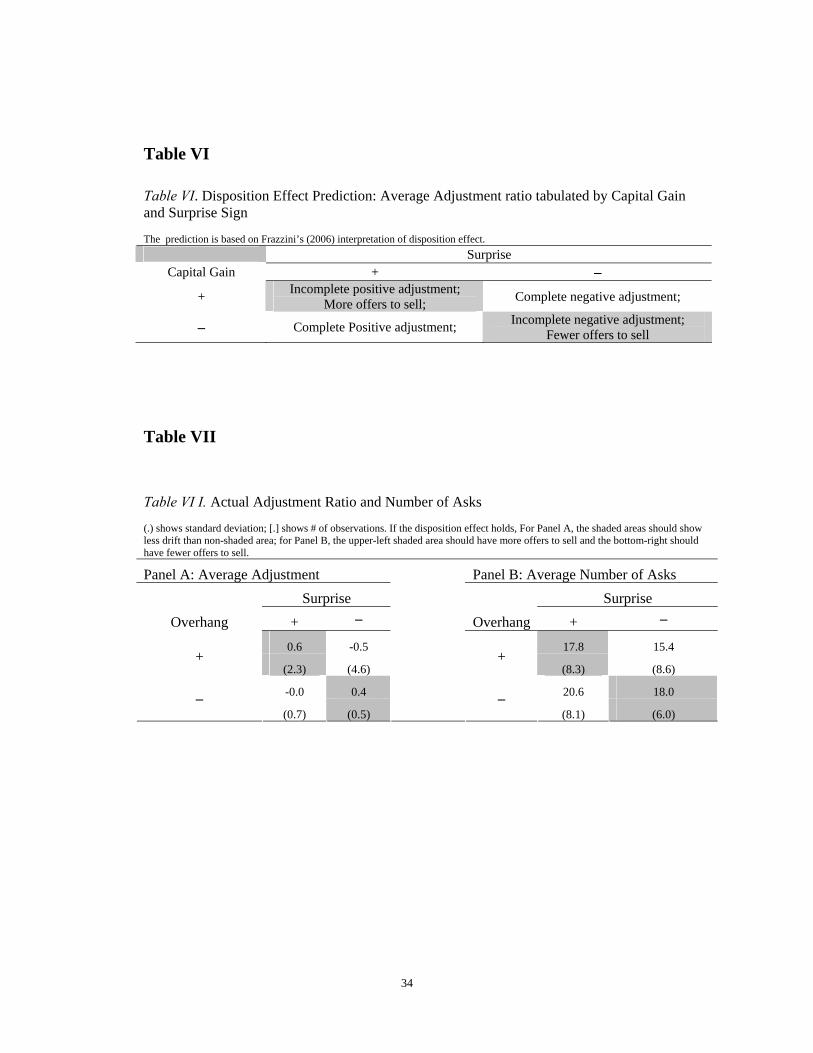
Table VI

Table VI. Disposition Effect Prediction: Average Adjustment ratio tabulated by Capital Gain and Surprise Sign The prediction is based on Frazzini’s (2006) interpretation of disposition effect.

Surprise Capital Gain + –

+ Incomplete positive adjustment; More offers to sell; Complete negative adjustment;

– Complete Positive adjustment; Incomplete negative adjustment; Fewer offers to sell

Table VII

Table VI I. Actual Adjustment Ratio and Number of Asks (.) shows standard deviation; [.] shows # of observations. If the disposition effect holds, For Panel A, the shaded areas should show less drift than non-shaded area; for Panel B, the upper-left shaded area should have more offers to sell and the bottom-right should have fewer offers to sell.

Panel A: Average Adjustment Panel B: Average Number of Asks Surprise Surprise

Overhang + –

Overhang + – 0.6 -0.5 17.8 15.4

+ (2.3) (4.6)

+ (8.3) (8.6)

-0.0 0.4 20.6 18.0 – (0.7) (0.5)

– (8.1) (6.0)

34

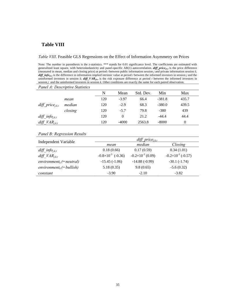
Table VIII

Table VIII. Feasible GLS Regressions on the Effect of Information Asymmetry on Prices Note: The number in parenthesis is the z-statistics. *** stands for 0.01 significance level. The coefficients are estimated with generalized least square, with heteroskedasticity and panel-specific AR(1) autocorrelation. diff_pricej,k,t is the price difference (measured in mean, median and closing price) at period t between public information session j and private information session k; diff_infoj,k,t is the difference in information implied intrinsic value at period t between the informed investors in session j and the uninformed investors in session k; diff_VARj,k,t is the risk exposure difference at period t between the informed investors in session j and the uninformed investors in session k. Other conditions are exactly the same for each paired observation.

Panel A: Descriptive Statistics N Mean Std. Dev. Min Max

mean 120 -3.97 66.4 -381.8 435.7 median 120 -2.9 68.3 -380.0 439.5 diff_pricej,k,t closing 120 -5.7 79.8 -380 439

diff_infoj,k,t 120 0 21.2 -44.4 44.4 diff_VARj,k,t 120 -4000 2563.8 -8000 0

Panel B: Regression Results

diff_pricej,k,t Independent Variable mean median Closing diff_infoj,k,t 0.18 (0.66) 0.17 (0.59) 0.34 (1.01) diff_VARj,k,t -0.8×10-3 (-0.36) -0.2×10-3 (0.09) -0.2×10-3 (-0.57) environmentk (=neutral) -15.45 (-1.06) -14.88 (-0.99) -30.1 (-1.74) environmentk (=bullish) 5.18 (0.35) 9.8 (0.65) -5.6 (0.32) constant -3.90 -2.10 -3.82

35

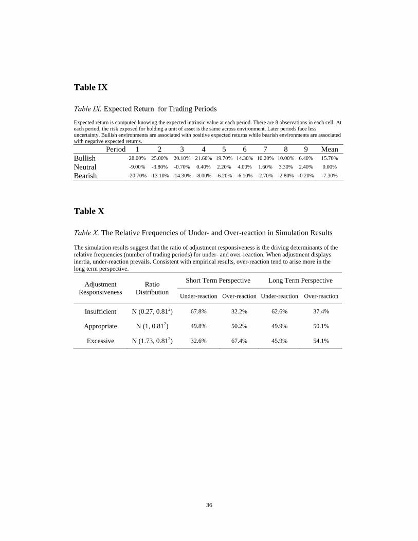
Table IX

Table IX. Expected Return for Trading Periods Expected return is computed knowing the expected intrinsic value at each period. There are 8 observations in each cell. At each period, the risk exposed for holding a unit of asset is the same across environment. Later periods face less uncertainty. Bullish environments are associated with positive expected returns while bearish environments are associated with negative expected returns.

Period 1 2 3 4 5 6 7 8 9 Mean Bullish 28.00% 25.00% 20.10% 21.60% 19.70% 14.30% 10.20% 10.00% 6.40% 15.70%

Neutral -9.00% -3.80% -0.70% 0.40% 2.20% 4.00% 1.60% 3.30% 2.40% 0.00%

Bearish -20.70% -13.10% -14.30% -8.00% -6.20% -6.10% -2.70% -2.80% -0.20% -7.30%

Table X

Table X. The Relative Frequencies of Under- and Over-reaction in Simulation Results The simulation results suggest that the ratio of adjustment responsiveness is the driving determinants of the relative frequencies (number of trading periods) for under- and over-reaction. When adjustment displays inertia, under-reaction prevails. Consistent with empirical results, over-reaction tend to arise more in the long term perspective.

Short Term Perspective Long Term Perspective Adjustment Responsiveness

Ratio Distribution Under-reaction Over-reaction Under-reaction Over-reaction

Insufficient N (0.27, 0.812) 67.8% 32.2% 62.6% 37.4%

Appropriate N (1, 0.812) 49.8% 50.2% 49.9% 50.1%

Excessive N (1.73, 0.812) 32.6% 67.4% 45.9% 54.1%

36

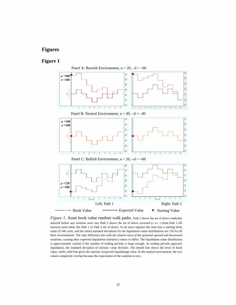
Figures

Figure 1 Panel A: Bearish Environment, u = 20, –d = –60

Starting Value Expected Value Book Value

Figure 1. Asset book value random walk paths. Path 1 shows the set of draws randomly selected before any sessions were run; Path 2 shows the set of draws reversed (+ ↔ −) from Path 1.All sessions used either the Path 1 or Path 2 set of draws. In all news regimes the asset has a starting book value of 540 cents, and the initial standard deviations for the liquidation value distributions are 120 for all three environments. The only difference lies with the relative sizes of the potential upward and downward surprises, causing their expected liquidation (intrinsic) values to differ. The liquidation value distribution is approximately normal if the number of trading periods is large enough. As trading periods approach liquidation, the standard deviation of intrinsic value declines. The dotted line shows the level of book value, while solid line gives the intrinsic (expected liquidating) value. In the neutral environment, the two values completely overlap because the expectation of the surprise is zero.

Left: Path 1 Right: Path 2

Panel B: Neutral Environment, u = 40, –d = –40

Panel C: Bullish Environment, u = 20, –d = –60

µ =720 σ =180

µ =540 σ =180

µ =360 σ =180

37

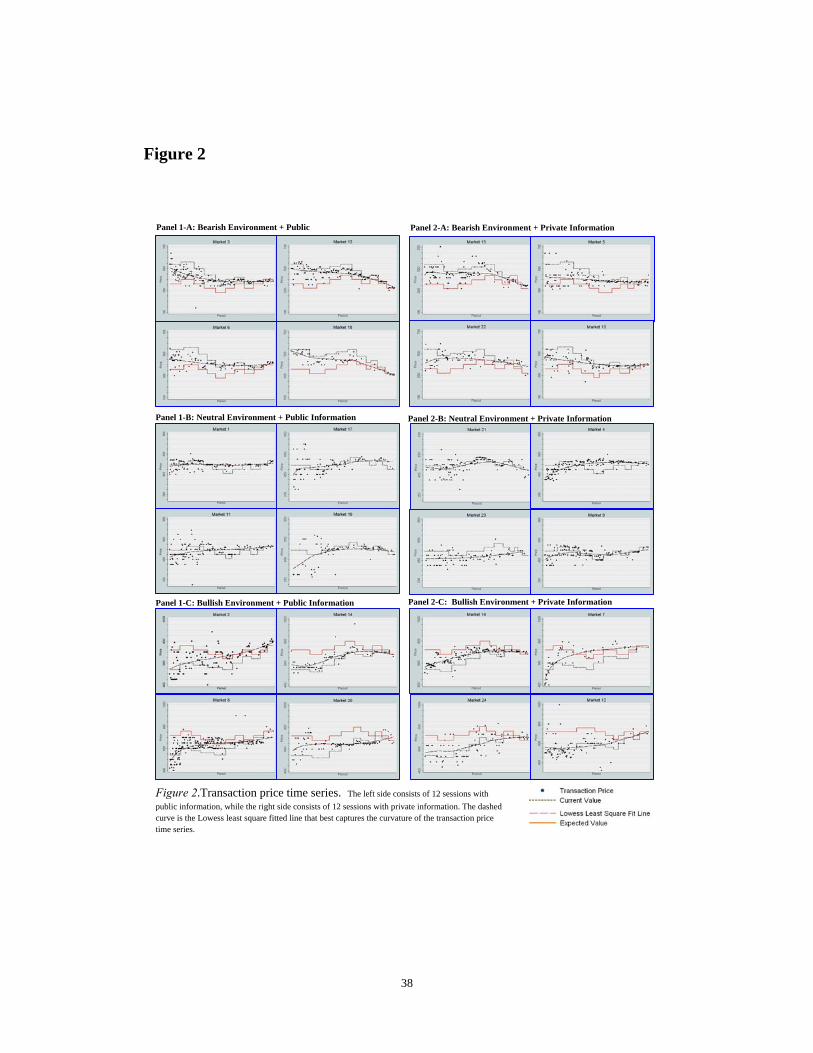
Figure 2

Figure 2.Transaction price time series. The left side consists of 12 sessions with public information, while the right side consists of 12 sessions with private information. The dashed curve is the Lowess least square fitted line that best captures the curvature of the transaction price time series.

Panel 1-A: Bearish Environment + Public

Panel 1-B: Neutral Environment + Public Information

Panel 1-C: Bullish Environment + Public Information Panel 2-C: Bullish Environment + Private Information

Panel 2-B: Neutral Environment + Private Information

Panel 2-A: Bearish Environment + Private Information

38

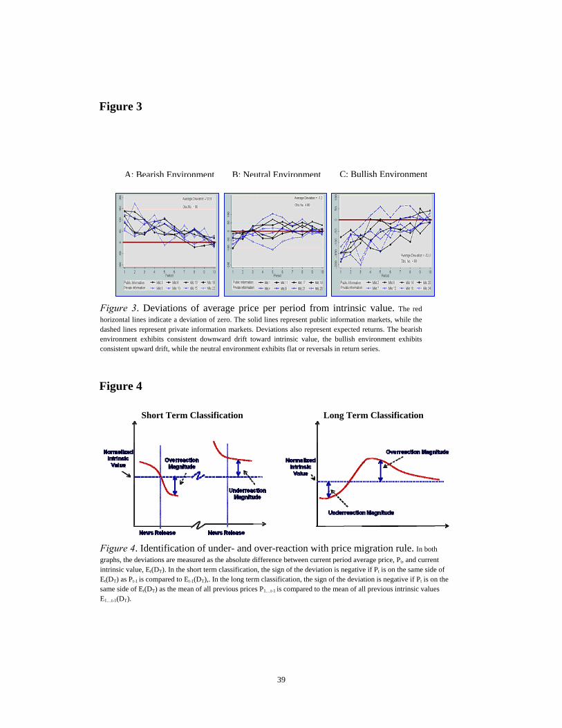
Figure 3

C: Bullish EnvironmentB: Neutral EnvironmentA: Bearish Environment

Figure 4

Long Term Classification Short Term Classification

Figure 3. Deviations of average price per period from intrinsic value. The red horizontal lines indicate a deviation of zero. The solid lines represent public information markets, while thedashed lines represent private information markets. Deviations also represent expected returns. The bearish environment exhibits consistent downward drift toward intrinsic value, the bullish environment exhibits consistent upward drift, while the neutral environment exhibits flat or reversals in return series.

Figure 4. Identification of under- and over-reaction with price migration rule. In both graphs, the deviations are measured as the absolute difference between current period average price, Pt, and current intrinsic value, Et(DT). In the short term classification, the sign of the deviation is negative if Pt is on the same side of Et(DT) as Pt-1 is compared to Et-1(DT),. In the long term classification, the sign of the deviation is negative if Pt is on the same side of Et(DT) as the mean of all previous prices P1…t-1 is compared to the mean of all previous intrinsic values E1…t-1(DT).

39

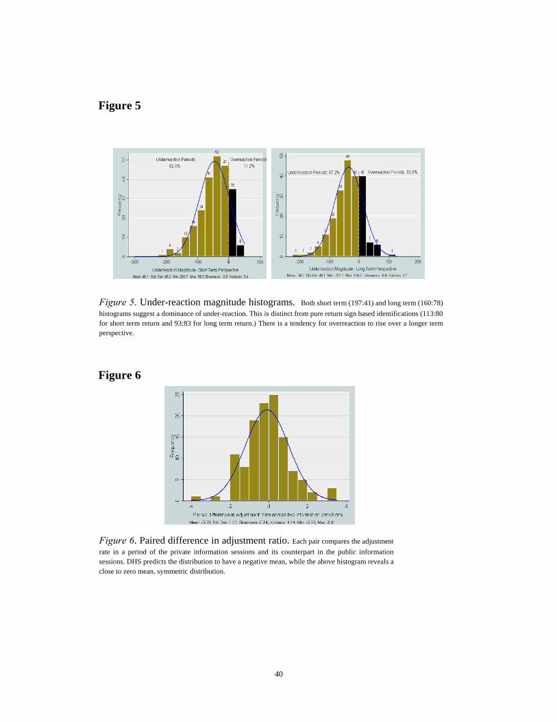
Figure 5

Figure 6

Figure 6. Paired difference in adjustment ratio. Each pair compares the adjustment rate in a period of the private information sessions and its counterpart in the public information sessions. DHS predicts the distribution to have a negative mean, while the above histogram reveals aclose to zero mean, symmetric distribution.

Figure 5. Under-reaction magnitude histograms. Both short term (197:41) and long term (160:78) histograms suggest a dominance of under-reaction. This is distinct from pure return sign based identifications (113:80for short term return and 93:83 for long term return.) There is a tendency for overreaction to rise over a longer term perspective.

40

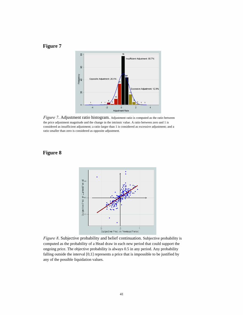
Figure 7

Figure 8

Figure 7. Adjustment ratio histogram. Adjustment ratio is computed as the ratio between the price adjustment magnitude and the change in the intrinsic value. A ratio between zero and 1 is considered as insufficient adjustment; a ratio larger than 1 is considered as excessive adjustment; and a ratio smaller than zero is considered as opposite adjustment.

Figure 8. Subjective probability and belief continuation. Subjective probability is computed as the probability of a Head draw in each new period that could support the ongoing price. The objective probability is always 0.5 in any period. Any probability falling outside the interval [0,1] represents a price that is impossible to be justified by any of the possible liquidation values.

41

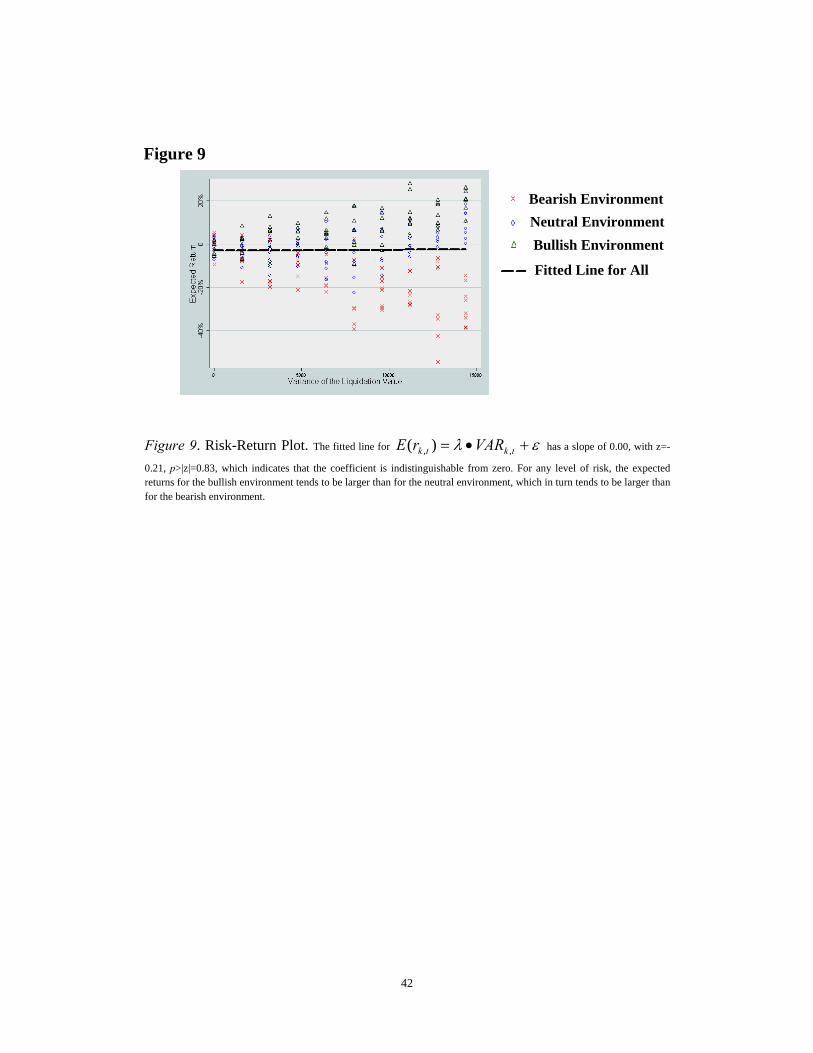
Figure 9

Fitted Line for All

Bullish Environment

Neutral Environment

Bearish Environment

Figure 9. Risk-Return Plot. The fitted line for  ελ +•= tktk VARrE ,, )(  has a slope of 0.00, with z=-

0.21, p>|z|=0.83, which indicates that the coefficient is indistinguishable from zero. For any level of risk, the expected returns for the bullish environment tends to be larger than for the neutral environment, which in turn tends to be larger thanfor the bearish environment.

42

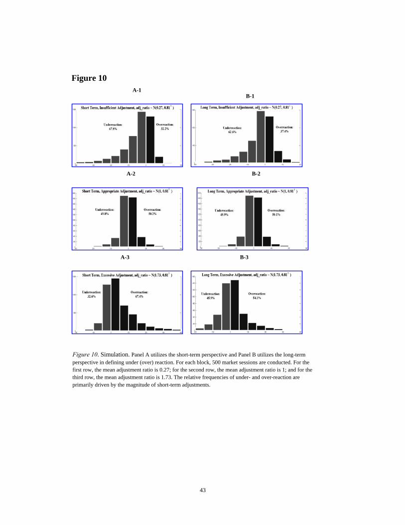
Figure 10 A-1

B-1

A-2

A-3

B-2

B-3

Figure 10. Simulation. Panel A utilizes the short-term perspective and Panel B utilizes the long-term perspective in defining under (over) reaction. For each block, 500 market sessions are conducted. For the first row, the mean adjustment ratio is 0.27; for the second row, the mean adjustment ratio is 1; and for the third row, the mean adjustment ratio is 1.73. The relative frequencies of under- and over-reaction are primarily driven by the magnitude of short-term adjustments.

43

Economic Science Institute Working Papers 

2010

10-03 Lin, S. Gradual Information Diffusion and Asset Price Momentum. 10-02 Gjerstad, S. and Smith, V. Household expenditure cycles and economic cycles, 1920 – 2010. 10-01 Dickhaut, J., Lin, S., Porter, D. and Smith, V. Durability, Re-trading and Market Performance.

2009

09-11 Hazlett, T., Porter, D., Smith, V. Radio Spectrum and the Disruptive Clarity OF Ronald Coase. 09-10 Sheremeta, R. Expenditures and Information Disclosure in Two-Stage Political Contests. 09-09 Sheremeta, R. and Zhang, J. Can Groups Solve the Problem of Over-Bidding in Contests? 09-08 Sheremeta, R. and Zhang, J. Multi-Level Trust Game with "Insider" Communication. 09-07 Price, C. and Sheremeta, R. Endowment Effects in Contests. 09-06 Cason, T., Savikhin, A. and Sheremeta, R. Cooperation Spillovers in Coordination Games. 09-05 Sheremeta, R. Contest Design: An Experimental Investigation. 09-04 Sheremeta, R. Experimental Comparison of Multi-Stage and One-Stage Contests. 09-03 Smith, A., Skarbek, D., and Wilson, B. Anarchy, Groups, and Conflict: An Experiment on the Emergence of Protective Associations.

09-02 Jaworski, T. and Wilson, B. Go West Young Man: Self-selection and Endogenous Property Rights.

09-01 Gjerstad, S. Housing Market Price Tier Movements in an Expansion and Collapse.

2008

08-10 Dickhaut, J., Houser, D., Aimone, J., Tila, D. and Johnson, C. High Stakes Behavior with Low Payoffs: Inducing Preferences with Holt-Laury Gambles.

08-09 Stecher, J., Shields, T. and Dickhaut, J. Generating Ambiguity in the Laboratory.

08-08 Stecher, J., Lunawat, R., Pronin, K. and Dickhaut, J. Decision Making and Trade without Probabilities.

08-07 Dickhaut, J., Lungu, O., Smith, V., Xin, B. and Rustichini, A. A Neuronal Mechanism of Choice.

08-06 Anctil, R., Dickhaut, J., Johnson, K., and Kanodia, C. Does Information Transparency Decrease Coordination Failure?

08-05 Tila, D. and Porter, D. Group Prediction in Information Markets With and Without Trading Information and Price Manipulation Incentives.

08-04 Caginalp, G., Hao, L., Porter, D. and Smith, V. Asset Market Reactions to News: An Experimental Study.

08-03 Thomas, C. and Wilson, B. Horizontal Product Differentiation in Auctions and Multilateral Negotiations.

08-02 Oprea, R., Wilson, B. and Zillante, A. War of Attrition: Evidence from a Laboratory Experiment on Market Exit.

08-01 Oprea, R., Porter, D., Hibbert, C., Hanson, R. and Tila, D. Can Manipulators Mislead Prediction Market Observers?