OXFORD BULLETIN OF ECONOMICS ANT) STATISTICS, 56,4 ( 1994) 0305-9049

ARE HIGHER LONG-TERM UNEMPLOYMENT RATES ASSOCIATED WITH LOWER

EARNINGS?

Neil Manning

1. INTRODUCTION

Over the past decade, there has been considerable interest in the relationship between unemployment and earnings in general, and the differing impacts Of long-term and short-run unemployment in particular. Layard and Nickell (1986, 1987), and Nickell (1987) were the first to emphasize the importance of duration and found no significant association between long-term unemployment and wages or wage inflation. Their conclusion, that only short-term unemployment affects wage determination, obviously has important labour market policy implications and is congruent with the notion of hysteresis in unemployment. This paper utilises data collected at the county level over the period 1983-02 to re-consider the roles of short-run and long-term unemployment in earnings determination. The results of estimating a dynamic model of earnings determination using the Generalized Methods of Moments approach of Arellano and Bond ( 1988) lend support to Layard and Nickell's conclusions.

The finding of a differential impact of short-run and long-term unemploy- ment on wage determination in Britain is challenged by few, and has been supported in empirical studies of single cross-sections from the General Household Survey, (Blackaby and Manning, 1990; Blackaby and Hunt, 1992); pooled cross sections from the Family Expenditure Survey (Blackaby el a/., 1991), and from pooled regional time series data (Blackaby and Manning, 1992). The econometric techniques used in these studies are diverse. There is error-correction modelling of time-series data, covariance analysis of pooled regional time series data, and the estimation from individual-level micro data of cross-sectional Mincer earnings functions with unemployment terms as additional regressors.

The micro data analyses have included controls for individual characteristics and the aggregate and regionat-level analyses have included

The author wishes to thank Steven Nickell and Andrew Oswald for helpful suggestions and David Blackaby and Stephen Jenkins for comments on an earlier draft of the paper. Any remaining errors are his own responsibility.

383 0 Basil Blackwell Ltd. 1994. Published by Blackwell Publishers, 108 Cowley Road, Oxford OX4 1JF, UK & 238 Main Street. Cambridgc. MA 021 42. USA.

384 BULLETIN

the influence of aggregate demand, cost of living and other effects. The apparent consensus on the inefectiveness of long-term unemployment in wage determination may seem surprising in view of the diversity of the above studies, both in terms of methodology and data sets analyzed.

However, Blanchflower and Oswald (1990) claim that this empirical consensus is largely an illusion and that it reflects model mis-specification. They consider the effect on wage determination of the long-term unemployed may be less than that of those who have been unemployed for shorter periods, but nevertheless, still exists. Indeed, Blanchflower and Oswald have claimed the 'wave curve' is non-linear with an upwards sloping section in which increases in the rate of unemployment are associated with increases in wages. A similar quadratic relationship is also found in Blackaby and Hunt (1992), but solely in terms of short-term unemployment. This latter study finds the effect of the long-term unemployed to be insignificant in a (single) cross-sectional earnings function which includes quadratic terms in both short-run and long-term unemployment together with a cross-product term.

One common feature of the data analyzed in this literature is the limited number of cross-section units - only ten standard CSO regions or a maximum of 24 regions/metropolitan areas are distinguished. Considerable intru-regional variation in unemployment rates is therefore masked by such coarse aggregation. To re-consider whether long-term unemployment fails to exert downward pressure on earnings, we use a quasi-panel of county data on earnings and unemployment rates for males taken from the published New Earnings Survey reports and NOMIS' respectively. The balanced panel comprises information from 60 of the 66 counties in England, Scotland and Wales over the ten year period 1983-l-9922. Given the large number of counties relative to the number of cross-sections together with the endogeneity of unemployment, the Generalized Methods of Moments estimator of Arellano and Bond (1988) is a natural choice for empirical analysis of these data. A data appendix provides full details of data definitions and sources.

We use two main regression specifications to assess the impact of unemployment and unemployment duration on earnings. First, a double logarithmic form is frequently used in the literature cited above and is also employed in the GMM estimates presented in Section 111. Secondly, we use a flexible functional form approach in which the continuous unemployment data are entered into earnings equations as a series of dummy variables, each defined for given intervals in the unemployment rate(s). This approach parallels the treatment in Blanchflower and Oswald (1993), who used a pooled sample of GHS microdata over time but do not distinguish unemploy- ment durations and only measure unemployment at the standard regional level.

Durham. 'NOMIS is the National On-line Manpower Information Service based at the University of

*See data appendix for details.

Q Basil Blackwell Ltd. 1994.

EARNINGS AND EMPLOYMENT DURATION 385 An important finding of this paper is that the dummy coefficients on long-

term unemployment are jointly insignificant, while those on short-run unemployment are highly significant and suggestive of a monotonically negative relationship between log earnings and short-run unemployment3. In other words, the Blanchflower and Oswald contention is questioned and the earlier conclusion of Layard and Nickel1 supported.

The economic specifications employed are discussed briefly in Section I1 and the main estimation results are summarized in Section 111. Concluding comments follow in Section IV.

II. ECONOMETRIC SPECIFICATIONS

The following simple linear dynamic specification forms the basis for subsequent estimation:

In E , = a,, + year dummies + (regional dummies) f + a I In El, - I 4- (12 In E;,- 2 +a31nSRU,+a, lnSRU,,_,+a,InSRU,~2+a,InLTUif + a7 In LTU,,- I + a, In LTU,_, + (1)

where E is nominal weekly earnings, SRU is the rate of short-run unemploy- ment and LTU is the rate of long-term unemployment (defined as having a continuous spells over 52 weeks4). The Q,,, intercepts are county-specific faed effects which subsume regional dummies and the year dummy coefficients are common to all counties. The interaction terms between rqionaf dummies and the time trend t represent specific regional time trends. These proxy the effect of regional-specific omitted variables which are trended.

The basic framework ( 1) may also be estimated in first difference form:

A In El, =B0 + regional dummies + year dummies + B , A In El , - , + PzA In El, - 2

+/?,A InSRUif+/?4A lnSRUif-, +&A InSRU,,-,+/I,A InLTU,,

+ 8, A In LTVil- I + /?HA In LTU,, - + At,, (2) This effectively removes non-modelled county-specific fixed effects a,, which are present in ( 1) and transforms the regional time trends into regional fixed effects. Preliminary results of estimating equation (1) (with regional dummies rather than the aOi fmed effects) produced high values of a I and a2, which summed to almost unity; the a I and a2 estimates are likely to be biased upwards given the correlation between the (omitted) county-level fixed effects and the lagged dependent variables. Therefore, the estimates of equation (2) only are discussed below.

'This is strictly true only when lagged earnings are included in the specification. However, there is no evidence for a negative relationship between long-term unemployment and earnings in any dummy variable specification.

'Short-term unemployment comprises durations up to and including 52 weeks.

Q Basil Blackwell Lfd. 1994.

386 BULLETIN

In the case of estimation in first differences, In E , - , is not a valid instru- ment and, in period t, valid instruments include all cross-sections dated t - 2 and earlier. These moment restrictions may be expressed as E ( E ~ , , t r i , - / ) = 0 for all instruments vi I - ) , with j > 1 as explained in Arellano and Bond (1988) and Greene (1993). Although the GMM approach is attractive in view of increased efficiency in estimation over standard IV, the extent to which all theoretical moment restrictions are exploitable is limited by the cross-section dimension of the panel and by limitations of the DPD program used to estimate equation (2). With these data, only two moment restrictions are able to be exploited so that when estimating (2), valid instruments in period 10 are cross sections for periods 7 and 8 (although in principle cross sections from t = 1 through to t = 8 are suitable).

All the results from the panel estimation reported below are robust to heteroscedasticity and limited moving average processes in the tic residuals. The GMM approach is not, however, robust to autocorrelation and so Arellano and Bond’s (1991) robust test for AR(2) processes is reported5. A Sargan test of overidentifying restrictions is also presented. Equation (2) includes region-specific dummies together with a set of time dummies which capture the influence of earnings determination of all factors measures at the national level such as movements in the retail price index. The inclusion of year dummies is a convenient method of dealing with the impact of schemes targeting the long-term unemployed which are obviously an important omitted factor in this analysis. If these schemes are national in coverage and ‘proportional’ in their effects, their impact will be picked up by the year dummies and will not bias the /I parameter estimates. County and region specific variation in other factors are not, however, taken into account except via the time trends in (1).

In the above analysis, a double logarithmic form is assumed6 but the relationship between earnings and unemployment may be re-assessed by entering unemployment as a series of dummy variables, each defined for a given rate of unemployment’. This approach is clearly non-parsimonious but does have the advantage of providing information on the form of the relationship between earnings and unemployment. As Blanchflower and Oswald have pointed out, the relationship may be non-linear and apparent duration dependence may in fact reflect inadequacies in the chosen functional form. This debate may be addressed by including both short-run and long-term unemployment via the dummy variable specification as in

51f the levels model (equation 1 ) is not autocorrelated, transforming to first differences removes the unobserved fixed effects but is likely to induce AR( 1 ) processes. In first differ- ences, the AR( 2) test is therefore appropriate.

“The number of variables included in equation ( 1 ) is limited but the qualitative nature of the conclusions is not affected by the choice of functional form. See Section 111.

‘The same approach is employed in Blanchflower and Oswald ( 1993) who also fail to find an upwards sloping section of the ’wage curve’ over the range of unemployment rates present in their sample.

0 Basil Blackwell Ltd. 1994.

EARNINGS AND EMPLOYMENT DURATION 387 equation (3) below:

In Elf= y,, + regional intercepts +year intercepts + yI In E , - I

where &ml,, and d / t ~ l , are dummy variables for short-run and long-term unemployment respectively. Twenty dummy variables d m l h are defined by splitting up short-term unemployment in equally spaced intervals (e.g. 2.0-2.49 percent, 2.5-2.99 percent with the omitted dummy representing short-run unemployment rates of below 2%). The dummies for overall and long-term unemployment are similarly defined, although the range of relevant unemployment rates differs according to the duration of unemployment under consideration.

we estimate three dynamic variants of the model with dummy variables; (i) with a single lag in log earnings included as in (3), (ii) with the lag omitted so the model is atemporal and (iii) with two lags in log earnings included to assess the robustness of the results to changes in the lag specification in earnings. For each of the above three dynamic structures, the included unemployment dummies also vary: (a) includes only the overall unemploy- ment dummy variables; (b) includes only the short-run and (c) only the long- term dummies. Equation (3) is therefore the 'unrestricted' model with a single 1% log earnings which includes dummies for both short-run and long-term unemployment, No lags in the unemployment dummies are considered. Furthermore, all

the dummy variable specifications are estimated by OLS since the models are clearly Over-parameterized and require an inordinate number of instruments - GMM estimation using the Arellano and Bond approach is not feasible given the number of counties in the sample.

+ Zldil dSmllr + Zld21 dltul,, + (3)

111. RESULTS

The results of estimating equation (2) by GMM which imposes a Common coefficient vector Over time and across regions are given in Table 1. Although the two-period lagged differences A In E,, - 2, A In SRUl,- 2 and A In LTUit- 2 were collectively insignificant in preliminary estimation, A In E,,- 2 is retained in the specification reported in Table 1 since omission induces autocorrela- tion which is just significant at the 95 percent level according to the Arellano and Bond AR(2) test. When A InSRUj,-2 and A InLTU,,-2 are omitted, there are no signs of mis-specification in the first-difference estimates. The instruments used are pjven in the table and include two moment restrictions on dl variables lagged at least two years. All results reported in Tables 1 and 2 are robust to heteroscedasticity and refer to two-step GMM estimates. See the notes to the tables for details.

In Table 1, the estimates of equation (2) are well determined with a clear negative influence of log short-term unemployment on log earnings and little

0 Basil Blackwcll Lld. 1994.

TABLE 1 Dynamic Panel Estimates

AlnE,,=B,,+year/region dummies+B,AlnEi,-, +@2AlnEil-2 +&AlnSRU, + @,AlnSRU,,_, + j15 A h LTUil+ jIn A h LTU,,-,

Variable Coeficient t-stat

A h E,- I A h Ei,-* A h SRU,l AlnSRU,,, I

A h L Wit Aln LTU,l-,

-0.3811 4.99 -0.0914 1.77

- 0.0688 - 0.0388

0.0589 - 0.0672

5.91 3.64

3.37 4.92

Long-run solution: In E-constants - 0.0731 InSRU- 0.0056 In LTU Diagnostic tests Sargan test (36) A R M

37.38 1.52

Wald tests Above regressors (6) 209.15' Time dummies (6) 286.24* Regional dummies (9) 136.43* Both dummies ( 15) 487.46* Significance of A LnLTu(2) 24.2 1 * Sample period 1983-92 Number of counties analyzed = 60 Number of years analyzed = 7 Degrees of freedom = 398 Instruments used - G(ln E,2,2), G(lnLTU,2,2), G(ln SRU,2,2), dummies Stability analysis

Coefficients -. 81982 8 3 - A 4 --A sub-groupl

1986 1987 1988 1989 1990 1991 1992 1986-89 5% critical value

1.28 3 1.80* 0.64

13.07* 17.28* 20.75* 5.89

24.27* 5.99

14.78* 17.13" 7.24

1 1.62* 18.24' 28.41* 24.58* 30.94. 9.49

21.12' 10.02 11.59 13.17* 11.33 10.36 17.73* 66.17* 12.59

Notes: The Wald and Sargan tests are all xz with the degrees of freedom stated on the table. Significant at the 95X level is denoted *. All f-statistics are robust to heteroscedasticity. The instruments used are denoted G(lnL.TU.2.2) to denote use of the logged rate of long term unemployed with a minimum lag of two periods and two moment restrictions being exploited. Thus in period 10, InLTU in periods 7 and 8 are used as instruments. The AR(2) tests statistics are asymptotically standard normal variables. The degrees of freedom for the Wald tests are 2 in column I , 4 in column 2 and 6 in column 3. Significance at the 95 percent level is denoted *.

EARNINGS AND EMPLOYMENT DURATION 389 TABLE 2

Dynamic Panel Estimates - Sample Break ul IW9

A In El,= B,, + yearlregion dummies + jf?, A In Ell- + PzA In El, - + P3 A In SRU,, + p4A In SRU,,-, + &A In LTU,,+ &,A in LTU,,-,

Estimation period I W6-89 Estimcition period 1090-92

Variable Coeficienr 1-stat (beficienr r-star ~.

A In El l - , - 0.400 I A In Ell.-2 0.0307

A In SRU,, -0.1065

A In L TU,, 0.0289 A In L TU,, - I - 0.0449

Long-run solutions: In E =constants -

A In SRU,-, 0.0220

4.03 0.46

4.9 1 1.03

0.92 I .93

-~ -~

- 0.7605 3.96 - 0.2738 4.17

0,0280 0.93 - 0.0722 3.56

0.01 17 0.44 - 0.0 1 14 0.55

0617 InSR- -0.01 17 InLTU( 1986-89) InE=constants-0.0218 InSRU+0.0001 In LTU(1990-92)

Diagnostic tests Sargan test (30)

Wald tests Above regressors ( 12) Time dummies (6) Regional dummies (9) Both dummies (15) Significance of A In L T u ( 4 )

AR (2) 32.32

1.92

245.27. 293.92*

86.72* 487.98*

4.74

evidence of a similarly negative influence of long-term unemployment on Furthermore, the regressors included and both sets of dummies are

hlghlY significant, but the long-run effect of long-term unemployment op earnings is effectively zero, despite the included variables being highly signifi- cant according to a Wald test. If anything, these results suggest that rises in long-term unemployment have a positive effect on earnings in the short-run, and a negligibly small negative impact in the long-run. This latter finding would Support the Nickell and Layard result as discussed in Section I.

The results above are derived assuming slope coefficients are constants Over regions and time. Stability Over the sample period is not an acceptable 'estriction as the summary results in the lower part of Table 1 illustrates. In

0 Basil Blackwell Ltd. 1994.

390 BULLETIN

TABLE 3 Static Least Squares Regressions

In E = a(, + regional dummies + a, In SRU + a, In LTU

tfetl BJ se Sub-group Her2 Reset R' Qo a, a,

1983 6.76* 0.86

1984 6.20* 1.19

1985 7.08* 1.12

1986 4.20' 1.42

1987 3.76 1.62

1988 3.65 1.22

1989 4.4 1 * 0.99

1990 5.43* 0.82

1991 6.66* 1.61

1992 7.29* 0.69

12.06* 0.70

18.95* 0.96

18.09" 0.14

14.26* 0.6 1 9.46* 0.27

20.73' 0.45

25.23* 0.20 8.84* 1.29 1.47 1.62 1.63 0.39

0.0554 0.3188 0.0585 0.3355 0.0533 0.4030 0.0626 0.3384 0.0638 0.3788 0.0608 0.5 107 0.06 18 0.5288 0.0636 0.5454 0.0633 0.5338 0.0593 0.5791

5.2434

5.2828

5.4147

5.5473

5.5426

5.6510

5.74 15

5.8666

6.05 18

6.2041

(99.26)

(97.27)

(101.82)

(103.62)

(1 59.8 1)

(173.61)

(1 93.95)

( 154.66)

(84.07)

(83.29)

- 0.0254

-0.0196 ( 1.42) - 0.03 15 (2.77) - 0.0287 (2.27) - 0.0339 (3.46) - 0.0538 (3.29) - 0.0542 (3.58) - 0.047 1 (3.46) - 0.0395 (3.48) - 0.0562 (4.62)

(2.22) 0.0177

(2.50) 0.0131

( 1.60) 0.0192

(3.34) 0.0 164

(2.50) 0.0205

(3.91) 0.0372

0.0430 (3.61) 0.0427

(3.02) 0.0378 (3.03) 0.0395

(3.59)

(3.73)

Notes. The diagnostics for the single equation cross-section are: Het 1, Heteroscedasticity in squared fitted values - F( 1.47); Het2, Heteroscedasticity in squared regressors - F( 13.35); BJ. Bera-Jarque test for normality of residuals - distributed ?(2); Reset, Ramsey reset test for linearity of functional form F( 1,47); se, standard error of regression; R 2 , adjusted RZ. All m a t s are robust to heteroscedasticity.

fact, considerable temporal instability in the coefficients is evident. In the lower section of Table 1, the first column presents Wald tests for uniform lag coefficients on In E , , the second column similar test results for uniformity of the coefficients on unemployment, and the final column report stability tests for all six estimated t9 coefficients. This instability is most noticeable when the sample is divided into two sub-periods, 1986-89 and 1990-92 (which not only divides the sample in half, but also coincides with the onset of recession). The results of separate estimation over these latter two subsamples are given in Table 2R. Although substantial variation in the estimates of equation (2) is evident between the two sub-periods, the same qualitative conclusions emerge: the coefficients summarizing the impact of long-term unemployment

"Some instability is also evident when the sample is divided by region. These results are not reported due to the small number of cross-section elements present.

0 Basil Blackwell Ltd. 1994.

EARNINGS AND EMPLOYMENT DURATION 391 are now collectively insignificant and the long-run elasticity of earnings with respect to short-run unemployment varies from - 0.06 in 1986-89 to - 0.02 in 1990-92.

In order to briefly reconsider the stability of the results over time, simple least squares regressions are run over single cross-sections and summary results are reported in Table 3. These estimates suffer from heteroscedasti- city and non-normality is apparent in all cases. Nevertheless, the results are very supportive of the original hypothesis - the negative relationship between unemployment and earnings is, in every cross-section, reflecting the influence of short-run rather than long-term unemployment.

The above estimation employs linear in logs specification throughout which may be inappropriate, as may the treatment of the duration of unemployment. Several reparameterizations were therefore considered, to assess the robustness of the overall findings to changes in functional form. The variations included transforming or not transforming to logarithms, including overall unemployment together with a duration term and including quadratic terms in unemployment. In each case, two lags in the earnings and unemployment variables were included, in contrast to the specification reported in Tables 1 and 2. In the interest of brevity, only the long-run results are presented below:

Equation constants not reported Long-run coe@'entsfrorn the two-step GMM estimates -

InE- -0.0751 InSRU-0.0041 lnLTUY lnEx -0,0188 SRU+0.0074 LTU 1nE=0.0465 In UN- 0.1 122 lnSRU In E = - 0.0?99 In UN+ 0.0043 In LTU E.= - 109.7851 SRU+ 15.5604 LTU E l -202.6749InSRU+87.5114LnLTU h E = -0.2196 I~SRU-0.0043 ( h S ~ U ) ~ - 0 . 0 0 8 4 lnLTU

In E = - 0.0404 SRU + 0.0001 SRU2 - 0.0046 LTU +0.0471 (1nLTU)'

+ 0.0022 LTU2 (2h) E=-434.1680 InSRU-20.8339(lnSRU)2+100.66641nLTU

+ 37.1361 (lnLTU)*

+ 0.7691 LTU2 (2i) E - - 19.8744 SRU- 0.5396 SRU2+ 11.1037 L W

Although considerable parameter variation is apparent in these long-run solutions, they are generally supportive of the main message of the paper. Only in case (2) is there any support for a negative influence of long-term

'Note the omission of A In SRU,,-, and A InLTU,,-, in Table 1 - these are both included in (2). The effect of this omission is slight - the long-nm elasticity of short-term

unemployment changes from - 0.073 to - 0.075. The effect of long-tern unemployment is unaffected

0 Basil Blackwell Ltd 1994.

0

m

1. I E :: h c € a P

e

W

W

0.05

(a)

All

unem

ploy

men

t

0.0

5.

0.05

'

(b)

Long

term

une

mpl

oym

ent

- 0.05

- 0

.05.

- 0.10

-0.1

0 '

w

\o

(c)

Shor

t ter

m u

nem

ploy

men

t N

- 0.05

.

-0.1

0,

..

..

..

..

..

..

..

..

1

Fig.

1.

Wag

e cu

rves

A

0.02

0 0.

020

L, +

0.02

0-

A

O.O

o0,

- o.O

o0

- 0.0

20

- 0.0

20

-0.W

. -0

.040

,

- 0.0

60

- 0.0

60

-0.m

0801

.

.

W

-0.0

80t

0.m

- 0.02

0

-0.0

40,

- 0.0

60

..

..

..

*

-0

.0

80

--

-

..

..

..

.

EARNINGS AND EMPLOYMENT DURATION 393

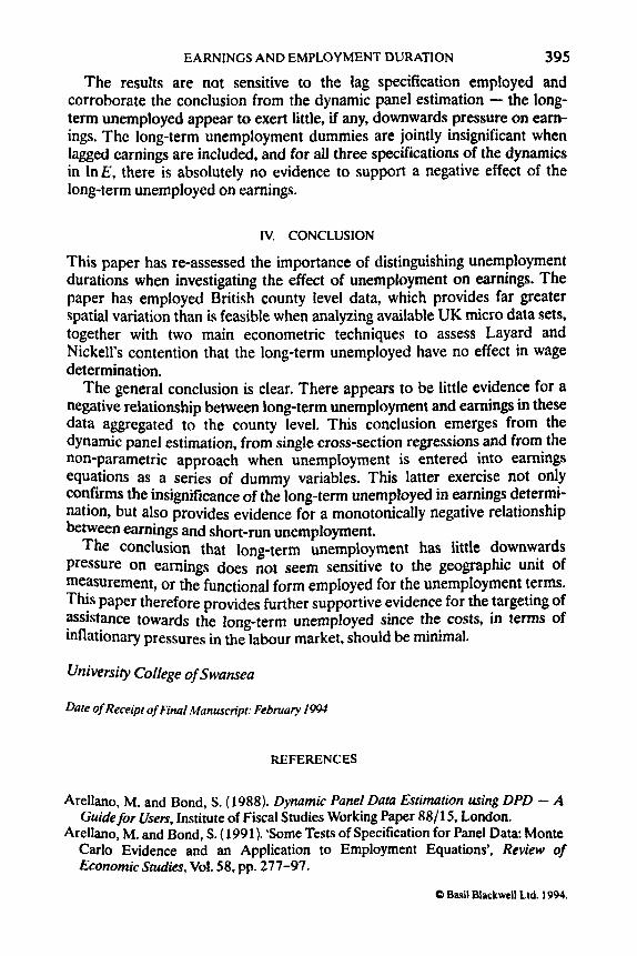
unemployment on earnings since in cases (2f) and (2g), the long-run elasticity of earnings with respect to long-term unemployment is positive for long-term rates above approximately 1 %lo. However, the unemployment dummy specifications such as equation (3) provide the most stringent test of the assumed functional form and summary results are presented graphically in Figure 1 (see also the notes to Figure 1 ).

The graphs in Figure 1 illustrate the dummy coefficients for static and single lag dynamic models as in equation (3) above in panels (a) and (d) when only the dummies for overall unemployment are included. The gaphs also produce a smoothed cubic function which is suggestive of a cubic 'Wage

A small number of 'Southern' counties have rates of male long-term unemployment below 1%. However, the number of such instances is low - the mean rate of long-term WemploYment i s 4.3 percent overall which varies from an average of 2.1 percent in 1990 to 5.8 percent in 1986. The maximum and minimum values in the complete sample afe 14.30 percent for Merseyside in 1986 and 0.3 percent for several South Eastern countles In 1990. In 1990, the Year with minimum long-term unemployment, a total of 13 out of 60 counttes had long-term rates below 1%.

I I1

Notes to Figure 1 In Figure 1, the results of estimating six versions of equation (3) are graphically summarized. The coefficients on the individual unemployment dummy variables are Plotted, together with the fitted value of regressing the dummy coefficients on cubic in the Unemployment dummies, i.e. a 'linear trend' for dummies 2 to 20 (one the omtted chss). Diagram (a) is based on the static regression:

In Ei,= yo + regional dummies + year dummies + 2,d) dun,,, those in panels (b) and (e) are based on: In '% = Yn + regional dummies + year dummies + z, I j dltujk+ z j d * j h m j i ,

~ ~ ~ e ~ ~ ~ m Y cod'ficients d,, are illustrated in panel (b), whilst the &j are shown in

Panels (d)-(f) repeat the above exercise, except that a single term in In ~ 1 , - is added to both the above specifications.

The equations fitted to the dummy coefficients on unemployment are: Figure panel Comtant t 1' x 10' t-' x 1 0 4 aa'j R2 (a) - 0.0461 - 0.01 70 0.2024 - 0,6232 0.5929

0.0171 0.9360 (b) 0.0478 -0.01 12 0.0129 -0.5087 0.9199 (4 -0.0018 -0.0051 0.1461 -0.1033 0.8390 (4 0.0325 - 0.0063 0.0438 -0.0522 0.9585 (e) 0.0145 - 0.0060 0.0266

(f) 0.0076 -0.0353 0.0238 - 0.097 1 0.59 13

are in parentheses. 't' refers to the 'number' of the dummy Coefficient on

0 Basil Blackwell Ltd. 1994.

(0.43) (3.75) (3.88) (3.64)

(1.98) (0.19) (0.08)

(0.15) (1 .04) (2.60) (2.75)

(8.46) (3.90) (2.36) (1.68)

(4.22) (4.15) ( 1.60) (0.96)

(1 -46) (0.16) (0.95) (1.18)

(3.55)

where t = 1,. . . ,19 (there are 20 dummies as explained above).

394 BULLETIN

curve’ in panel (a). This is apparently supportive of the BlancMower and Oswald non-monotonic wage curve, but is sensitive to the specification. Including a single lag in earnings effectively restores monotonicity as illustrated in panel (d).

However, the main focus of attention here is on the importance of duration. Therefore, the results of fitting static and dynamic variants of equation (3) - which includes both the short-run and long-term dummies - are also reproduced in Figure 1. In panels (b) and (e), the coefficients on the long-term unemployment dummy variables are graphed, together with the smoothed functions, and in (c) and (f), the short-run unemployment dummy coefficients are depicted. The vertical scales depict the dummy coefficient values, and these scales are common to panels (a)-(c) and to (d)-(f).

The crucial result is common to panels (b)-(c) and (e)-(f): the long-term unemployment dummies do not suggest a negative relationship between long- term unemployment rates and earnings and are jointly insignificant when lags in log earnings are included as the results summarized in Table 4 illustrate. The first column shows which dummies are included, the second column the employed lag length in log earnings and the residual sum of squares is denoted ‘RSS’ in column 4. Central to this paper is the role of duration which may be assessed by comparing the restricted specifications 2 and 3 against the unrestricted specification 4:

TABLE 4 Summary Results for Earnings Equations with Unemployment Dummies included

Hypothesis tests against Included Lag length Number of unrestricted equation (3) dummies in In E observations RSS in text (4 in Table)

1. un 0 600 1.9559 - 2. sm 0 600 2.0445 F(19,543)- 1.81* 3. ltu 0 600 2.0834 F( 19,543) = 2.39** 4. sru&Itu 0 600 1.9226 -

1. un 1 540 0.1826 - 2. S N 1 540 0.1820 F( 19,483) = 0.99 3. Itu 1 540 0.1901 F(19,543)=2.16** 4. sru&ltu 1 540 0.1752 - 1. un 2 480 0.1493 - 2. S N 2 480 0.1501 F(19,423)-0.74 3. Itu 2 480 0.1590 F( 19,423)=2.10** 4. sru&ltu 2 480 0.1453 -

Significance at the 95% level is denoted *, Fl),,)5( 1 9 , ~ ~ ) - 1.59. Significance at the 99% level is denoted **, F,, ( 1 9 , ~ ~ ) - 1.90.

0 Basil Blackwell Lid. 1994.

EARNINGS AND EMPLOYMENT DURATlON 395 The results are not sensitive to the lag specification employed and

corroborate the conclusion from the dynamic panel estimation - the long- term unemployed appear to exert little, if any, downwards pressure on earn- ings. The long-term unemployment dummies are jointly insignificant when lagged earnings are included, and for all three specifications of the dynamics in In E, there is absolutely no evidence to support a negative effect of the long-term unemployed on earnings.

IV. CONCLUSION

This paper has re-assessed the importance of distinguishing unemployment durations when investigating the effect of unemployment on earnings. The paper has employed British county level data, which provides far greater spatial variation than is feasible when analyzing available UK micro data sets, together with two main econometric techniques to assess Layard and Nickell’s contention that the long-term unemployed have no effect in wage determination.

The general conclusion is clear. There appears to be little evidence for a negative relationship between long-term unemployment and earnings in these data aggregated to the county level. This conclusion emerges from the dynamic panel estimation, from single cross-section regressions and from the non-parametric approach when unemployment is entered into earnings equations as a series of dummy variables. This latter exercise not Only confirms the insignificance of the long-term unemployed in earnings determi- nation, but also provides evidence for a monotonically negative relationship between earnings and short-run unemployment.

The conclusion that long-term unemployment has little downwards pressure on earnings does not Seem sensitive to the geographic Unit Of measurement, or the functional form employed for the unemployment terms. This Paper therefore provides further supportive evidence for the targeting Of assistance towards the long-term unemployed since the costs, in terms Of inflationary pressures in the labour market, should be minimal.

University College of Swansea

Dare of Receipt of Final Manuscript: February 1994

REFERENCES

Arellano, M. and Bond, S. (1988). Dynamic Panel Data Estimation using DPD - A Guide for Users, Institute of Fiscal Studies Working Paper 88/15, London.

Arellano, M. and Bond, S. (1991). ‘Some Tests of Specification for Panel Data: Monte Carlo Evidence and an Application to Employment Equations’, Review of EconomicStudies, Vol. 58, pp. 277-97.

0 Basil Blackwcll Ltd. 1994.

396 BULLETIN Blackaby, D. H., Bladen-Hovell, R and Symons, E. (1991). ‘Unemployment,

Duration and Wage Determination in the U K Evidence from the FES 1980-86‘,

Blackaby, D. H. and Hunt, L. C. (1992). ‘The “Wage Curve” and Long-Term

Blackaby, D. H. and Manning, N. (1990). The North-South Divide - Questions of

Blackaby, D. H. and Manning, N. (1992). ‘Regional Earnings and Unemployment -

BlancMower, D. G. and Oswald, A. ( 1990). The Wage Curve’, Scandinavian Journal

BlancMower, D. G. and Oswald, A. (1993). Estimating a UK Wage Curve 1973-m,

Greene, W. IL ( 1993). Econometric Analysis (second edition), Macmillan, Oxford. Layard, R and Nickell, S. (1986). ‘Unemployment in Britain’, Econornica, Vol. 53.

supplement, pp. S 12 1-69. Layard, R. and Nickell, S. (1987). ‘The Labour Market’, in Dornbusch, R. and

Layard, R. (eds.), The Performance of the Brithh Economy, Clarendon Press, Oxford.

Nickell, S. (1987). ‘Why is Wage Inflation in Britain So High?, BULLETIN, Vol. 49, pp. 103-28.

BULLETIN, Vol. 53, pp. 377-400.

Unemployment: A Cautionary Note’, Manchester School, Vol. 60, pp. 4 19-28.

Existence and Stability’, Economic Journal, Vol. 100, pp. 510-27.

A Simultaneous Approach’, BULLETIN, Vol. 53, pp. 481-502.

of Economics, Vol. 92, pp. 483-96.

mimeo.

DATA APPENDIX

The Earnings figures are taken from the New Earnings Survey reports, part E, various issues. The definition of Earnings is ‘Full-time males on adult rates, whose pay for the survey period was not affected by absence’. See New Earnings Survey, 1992, Part E, Table 110.

Interpolation of the earnings figure for Highlands (Scotland) in 1991 was required to provide a balanced panel of 60 counties over period 1983-92. This interpolation involved regressing the Highlands earnings on that for all other Scottish Counties in the sample for the period 1983-90 together with 1992 and taking the predicted value as the missing value for 1991. The Highlands earnings figures were not reported in the New Earnings Survey Reports due to high standard errors.

The unemployment figures are for males only, July figures (except for 1983, when the October figure was taken), and were taken from NOMIS, series WQAD, and use the workforce base in rate calculation. Earlier figures have rates calculated on the narrow base. Adjusting and splicing the two series to provide a sample from 1978 proved unsuccessful. The unemploy- ment rates for Surrey are unavailable and, on the basis of earlier available figures, were assumed equal to the rate for West Sussex.

South Ear? ( 12): Bedfordshire, Berkshire, Buckinghamshire, East Sussex, Essex, Greater London, Hampshire, Hertfordshire, Kent, Oxfordshire, Surrey and West Sussex.

The Counties included in the sample are:

0 Basil BlackweU Ltd. 1994.

Lothian, Strathclyde, Tayside.

Q Basil Bladtwcll Ltd 1994.