Arctic Sea Ice Seasonal Prediction by a Linear Markov Model

XIAOJUN YUAN

Lamont-Doherty Earth Observatory, Columbia University, Palisades, New York

DAKE CHEN

State Key Laboratory of Satellite Ocean Environment Dynamics, SIO/SOA, Hangzhou, China, and

Lamont-Doherty Earth Observatory, Columbia University, Palisades, New York

CUIHUA LI AND LEI WANG

Lamont-Doherty Earth Observatory, Columbia University, Palisades, New York

WANQIU WANG

Climate Prediction Center, National Centers for Environmental Prediction, College Park, Maryland

(Manuscript received 4 December 2015, in final form 3 August 2016)

ABSTRACT

A linear Markov model has been developed to predict sea ice concentration (SIC) in the pan-Arctic region at

intraseasonal to seasonal time scales, which represents an original effort to use a reduced-dimension statistical

model in forecasting Arctic sea ice year-round. The model was built to capture covariabilities in the atmosphere–

ocean–sea ice systemdefined by SIC, sea surface temperature, and surface air temperature.Multivariate empirical

orthogonal functions of these variables served as building blocks of themodel.A series ofmodel experiments were

carried out to determine the model’s dimension. The predictive skill of the model was evaluated by anomaly

correlation and root-mean-square errors in a cross-validated fashion . On average, the model is superior to the

predictions by anomaly persistence, damped anomaly persistence, and climatology. Themodel shows good skill in

predicting SIC anomalies within theArctic basin during summer and fall. Long-term trends partially contribute to

the model skill. However, the model still beats the anomaly persistence for all targeted seasons after linear trends

are removed. In winter and spring, the predictability is found only in the seasonal ice zone. The model has higher

anomaly correlation in the Atlantic sector than in the Pacific sector. The model predicts well the interannual

variability of sea ice extent (SIE) but underestimates its accelerated long-term decline, resulting in a systematic

model bias. This model bias can be reduced by the constant or linear regression bias corrections, leading to an

improved correlation skill of 0.92 by the regression bias correction for the 2-month-lead September SIEprediction.

1. Introduction

The rapid summer Arctic sea ice retreat has not only

been an icon of climate change but has also created more

commercial opportunities in the newly opened Arctic

waters, such as shipping and oil drilling (Eicken 2013).

However, lower summer sea ice cover comes with

larger ice variability (Goosse et al. 2009), causing tre-

mendous difficulties in planning, and even threatening,

commercial operations in theArctic. Therefore, skillful

sea ice prediction will become a needed service in the

warming Arctic environment. The scientific questions

that we are currently facing are the following: 1) To

what extent are sea ice anomalies from year to year

predictable, and 2) what skill do stochastic models have

beyond the information in the long-term trend, anom-

aly persistence, or climatology?

Sea ice is a fully interactive component of the climate

system. Sea ice concentration (SIC), extent, and thickness

Supplemental information related to this paper is available at the

Journals Online website: http://dx.doi.org/10.1175/JCLI-D-15-0858.s1.

Lamont-Doherty Earth Observatory Contribution Number 8062.

Corresponding author address: Xiaojun Yuan, Lamont-Doherty

Earth Observatory, 61 Rt. 9W, Palisades, NY 10964.

E-mail: xyuan@ldeo.columbia.edu

15 NOVEMBER 2016 YUAN ET AL . 8151

DOI: 10.1175/JCLI-D-15-0858.1

� 2016 American Meteorological Society

can vary on many different time scales, from intra-

seasonal, seasonal, interannual, to decadal and longer.

Many studies have shown that sea ice variations are

predominantly caused by atmospheric circulation

changes (Fang and Wallace 1994; Deser et al. 2000;

Pfirman et al. 2004; Wu and Zhang 2010). Proshutinsky

and Johnson (1997) suggest that theArctic winter sea ice

variability is forced by changes in the location and in-

tensity of the Icelandic low and the Siberian high.

Francis andHunter (2007) reveal that the Bering Sea ice

variability is influenced mainly by anomalies in easterly

winds associated with the Aleutian low, whereas the

Barents Sea ice variability is driven primarily by sea

surface temperature (SST) and local meridional winds.

Near theAlaska coastal region, the rapid sea ice decay is

related to downward solar radiation and mechanical

breakup due to winds and ocean currents following the

thermal weakening of sea ice, which leads to sea ice

predictability up to two weeks in advance (Petrich et al.

2012). A number of studies found that Arctic Oscillation

variability affects Arctic sea ice on a broad range of

time scales, ranging from seasonal to decadal (Deser

et al. 2000; Rigor et al. 2002; Serreze et al. 2003; Rigor

and Wallace 2004). Other low-frequency large-scale

climate patterns (e.g., NAO, PNA, ENSO, Arctic di-

pole) also exert a strong impact on Arctic sea ice

(Mysak et al. 1996; Mysak and Venegas 1998; Moritz

et al. 2002; L’Heureux et al. 2008; Wang et al. 2009).

These findings suggest that sea ice predictability likely

lies in the covariability of the polar climate system.

They imply that Arctic sea ice could be better pre-

dicted by empirical models when developed in the

multivariate space.

Sea ice itself is a relatively slow-varying component in

the atmosphere–ocean–sea ice coupled system, and SIC

anomalies usually persist for a few seasons (Chapman

and Walsh 1991; Yuan 2004). These characteristics

suggest that sea ice has a certain level of natural pre-

dictability. A good example is the seasonal forecast of

the Antarctic sea ice by a linear Markov model (Chen

and Yuan 2004). The success of the model is attributed

to the dominance of the Antarctic climate variability

by a few distinctive modes in the atmosphere–ocean–sea

ice coupled system, and to the model’s ability to pick up

these modes. In the Arctic, a number of studies suggest

that the summer sea ice may be predictable at a seasonal

time scale because of links between summer sea ice

condition and early season climate indices (Walsh and

Zwally 1990; McPhee et al. 1998; Maslanik et al. 1999;

Kwok 2000; Zhang et al. 2000; Drobot and Maslanik

2002). Chapman and Walsh (1991) found that an Arctic

sea ice anomaly can persist for several months but a

simple analog model has a meaningful skill of only one

month. Drobot andMaslanik (2002) were able to predict

sea ice anomaly in the Beaufort Sea a few months in

advance by using a linear regression model. A few sim-

ilar regression forecast models have been developed in

the Beaufort and Chukchi Seas (Drobot 2003), in the

Hudson Strait (Gough and Houser 2005), and for the

pan-Arctic summer sea ice minimum extent (Drobot

et al. 2006). This type of sea ice prediction model com-

monly uses themultiyear ice gradient, ice concentration,

air temperature, and climate indices like the NAO index

as predictors. Gough and Houser (2005) also found that

the oceanic heat gain or loss during previous seasons,

which is determined by the length of ice-free or ice-

covered season, is fundamentally important to the re-

gional forecast.

While the majority of statistical models were de-

veloped mostly for isolated regions or specific seasons,

coupled climate models, on the other hand, are able to

predict sea ice concentration and ice thickness at pan-

Arctic grid points and for all seasons. Many dynamic

models show some predictive skill at seasonal to in-

terannual time scales (Collins 2002; Koenigk and

Mikolajewicz 2009; Blanchard-Wrigglesworth et al.

2011a,b; Chevallier et al. 2013; Guemas et al. 2014;

Tietsche et al. 2014). For predicting September Arctic

sea ice extent (SIE), Lindsay et al. (2008) found that sea

ice concentration is the best predictor in the first two

months, while the ocean temperature at 200–270m is

more important for longer lead-time prediction in their

ice–ocean coupled model. In addition, studies revealed

that sea ice anomalies in melting seasons reemerge in

freezing seasons in multiple models, which is caused by

the persistence of SST anomalies near the ice edge

(Blanchard-Wrigglesworth et al. 2011a; Day et al. 2014;

Bushuk et al. 2014, 2015). Chevallier et al. (2013) found

that the Centre National de Recherches Météor-ologiques Coupled Global Climate Model has signifi-

cant skill in predicting the Arctic SIE in September even

after the linear trend was removed. On the other hand,

the prediction skill for theArctic sea ice extent was often

masked by the effect of long-term trends in other cou-

pled climate models (Lindsay et al. 2008; Sigmond et al.

2013; Msadek et al. 2014). Moreover, regional sea ice

prediction skill from dynamic models was evaluated

far less thoroughly at intraseasonal and seasonal

time scales.

Although there are limitations to sea ice predictability

owing to inherent chaotic atmospheric variability in the

Arctic climate system (Holland et al. 2010; Blanchard-

Wrigglesworth et al. 2011b), the above studies suggest

that it is feasible to predict Arctic sea ice at intraseasonal

to seasonal time scales. Despite great efforts toward

predicting the September total SIE through the sea ice

8152 JOURNAL OF CL IMATE VOLUME 29

prediction network (http://www.arcus.org/sipn), sea-

sonal or intraseasonal predictions for either the total ice

extent or ice concentration at grid points are very lim-

ited in other months in the pan-Arctic region. Skillful

sea ice forecast in the Arctic is still lacking even though

the demand for such prediction has grown tremendously

in recent decades. Because of its cost-effectiveness, we

are motivated to develop more advanced statistical

models for sea ice prediction in the pan-Arctic region.

In this study, we construct a linear Markov model for

monthly SIC at pan-Arctic grid points for all seasons.

The sea ice predictability is assessed at different loca-

tions and over all seasons. Through development of the

model, we isolate the relative importance of different

processes that dictate sea ice variability. In addition, we

generate SIE forecasts based on predicted SIC and

evaluate SIE prediction skill, with emphasis on the

September SIE.

2. Data and methodology

In this study, we primarily use SIC data from the

GSFC bootstrap SMMR–SSM/I version-2 quasi-daily

time series from 1979 to 2013 (Comiso 2000). This 35-yr

time series can be obtained from the EOS Distributed

Active Archive Center (DAAC) at the National Snow

and IceData Center (NSIDC; http://nsidc.org). Monthly

sea ice concentrations from original 25 km3 25 km grids

were bin-averaged into 28 3 0.58 longitude–latitude

grids. Atmospheric variables are taken from NCEP–

DOEAMIP-II reanalysis data with spatial resolution of

2.58 3 2.58. This dataset has been improved from the

original NCEP–NCAR reanalysis (Kalnay et al. 1996;

Kistler et al. 2001) by fixing errors and updating the

parameterization of the physical process in the model

(Kanamitsu et al. 2002; http://www.cpc.ncep.noaa.gov/

products/wesley/reanalysis2/kana/reanl2-1.htm). In ad-

dition, we use SST from Hadley Centre Sea Ice and Sea

Surface Temperature (HadISST) monthly data. The SST

data were reconstructed from in situ observations and sat-

ellite measurements from various sources with a spatial

resolutionof 18 3 18 longitude–latitude (Rayner et al. 2003).To isolate which oceanic and atmospheric variables

are closely related to sea ice variability, we calculated

correlations between SIC and the following: SST, sur-

face air temperature (SAT), pressure and winds at sea

level, and geopotential heights and winds at 500-hPa and

300-hPa levels, at collocated grid points. On average,

SIC is highly related to SST and SAT, followed by

geopotential height at 300 hPa, and then geopotential

height at 500 hPa, as well as winds at these levels. The

correlations with sea level pressure and surface winds

are relatively small. Because of the barotropic nature

of the polar troposphere (Ting 1994; Chen 2005), only

one pressure level in the troposphere is chosen.

Therefore, SIC, SST, SAT, and geopotential height

and winds at 300 hPa are chosen to form the initial

multivariate space for capturing the predictable vari-

ability in the atmosphere–ocean–sea ice system. A

linear Markov model is then constructed in the mul-

tivariate EOF (MEOF) space. The base functions of

the model’s spatial dependence consist of the eigen-

vectors from the MEOF of these six variables, while

the temporal evolution of the model is a Markov pro-

cess with its transition functions determined from the

corresponding principal components (PCs). We use

only several leading MEOF modes, which greatly re-

duce model space and filter out unpredictable small-

scale features. Similar Markov models have been used

to predict Antarctic sea ice (Chen and Yuan 2004), El

Niño–Southern Oscillation (ENSO; Blumenthal 1991;

Xue et al. 1994; Canizares et al. 2001; Xue et al. 2000),

and East Asian monsoon (Wu et al. 2013). Here, we

follow Chen and Yuan (2004) and construct a similar

model for seasonal prediction of Arctic sea ice

concentrations.

First, we create anomaly time series of SIC, SST, and

atmospheric variables from 1979 to 2012 by subtracting

climatologies of the same period from monthly mean

data and normalizing all anomaly series. The normali-

zation is applied to time series at grid points but does not

account for the differences in the numbers of grid points

for each variable. The number of grid points is 6728 for

SIC, 5040 for SST, and 3024 for each atmospheric vari-

able. To emphasize sea ice variability in the model

construction, we weight SIC, SST, SAT, 300-hPa height,

and u and y at the 300-hPa level by 2, 1, 1, 1, 1, and 1,

respectively, although the final model skill is not very

sensitive to the weight. The weighted variables are

stacked up into a single matrix V(n, m), where n is the

number of grid points of all fields and m is the length of

time series. We then decomposed V into eigenvectors

(spatial pattern) E and their corresponding PCs (time

series) P:

V5EPT , (1)

where the columns of E are orthogonal and the columns

of P are orthogonal; the superscript T denotes matrix

transposition. By truncating (1) to the first several

modes, we greatly reduce the model space. The Markov

model is computed using the single-step correlation

matrix—that is, a transition matrix A that satisfies the

following linear relationship:

Pi11

5APi1 e

i(2)

15 NOVEMBER 2016 YUAN ET AL . 8153

where i denotes the ith month and ei is the error in the

model fit. Multiplying (2) with PTi and averaging over

time yields the following:

hPi11

PTi i5AhP

iPTi i1 he

iPTi i , (3)

where angle brackets indicate time averaging. There

should be no correlation between ei and PTi for the best

model fit, so A can be calculated as follows:

A5Pi11

PTi Pi

(PTi )

21 . (4)

Since sea ice behaves dramatically differently in differ-

ent seasons,A needs to be considered season dependent;

thus (4) is actually applied to 12 subsets of PCs to obtain

different transition matrices for each of the 12 calendar

months. When the model is constructed, the sea ice

prediction will be made through following four steps:

1) the PCs corresponding to the initial anomalous cli-

mate conditions are calculated by projecting observa-

tions to the eigenvectors E, 2) the predictions of the PCs

are made at increasing lead times by successively ap-

plying the transition matrices, 3) the predicted PCs are

combined with the respective eigenvectors to forecast

sea ice concentration anomalies, and 4) the predicted

sea ice anomaly field is finally added into the climatology

to produce the final prediction.

To determine model variables that need to be used

in the model, we calculate the model’s hindcast skill

measured by anomaly correlation (AC) and root-

mean-square errors (RMSEs) between predictions and

observations. For hindcast experiments, the model is

initialized from each month of the 34 yr of time series,

and 12-month predictions aremade from each initialized

month. The hindcast skill in this study is equivalent to a

reconstructed time series skill (or in-sample skill). The

model variables are then determined by trial and error

based on hindcast skill averaged over 34 years. The

MEOF is recalculated each time when a new variable is

added. When we determine the model dimension, we

evaluate the model skill in a cross-validation fashion. To

avoid artificial skill, we subtract one year from PCs and

recalculate the transition matrix in (4); then we make

12-month predictions for that year. Here we subtract

one year of data from PCs instead of the original time

series because the spatial patterns of leading modes re-

main essentially the same when one year of data is taken

out from 34 yr of time series. The process is repeated for

each year of the time series. In this process, theMEOF is

not recalculated and the time series of PCs are reduced

to 33 years. Therefore, with slightly shorter time series,

the model prediction skill is assessed over 34 one-year

predictions. The cross-validated evaluation is stricter than

the hindcast assessment since the predicted year informa-

tion was not included in the Markov model construction.

In addition, the hindcast skill and cross-validated

skill are also compared to the skill of the SIC anomaly

persistence, damped anomaly persistence, and clima-

tology predictions. To be consistent with the hindcast

skill, the persistence function is constructed as follows:

the autocorrelations of SIC anomalies at each grid

point are computed from 1- to 12-month lag starting

from each month of the 34-yr time series and then are

averaged as a function of lag month. Damped anomaly

persistence provides a forecast that amplitudes of the

anomalies are assumed to reduce in time exponentially

at a time scale of the local autocorrelation. It is defined as

ndp(t)5 n(0)e2at, where n(0) is the initial anomaly, t is the

lead time, and the slope a is determined by the system’s

autocorrelation (Griffies and Bryan 1997). The damped

persistence is also calculated and averaged in the same

fashion as the anomaly persistence.

3. Arctic sea ice variability and MEOF analysis

Sea ice concentration and its total extent exhibit sig-

nificant declining trends in all seasons (Parkinson and

Cavalieri 2012; Simmonds 2015). During the period

from 1979 to 2012, ice concentration trends vary greatly

in space and are particularly large in the Barents Sea, in

the Kara Sea, and north of the Chukchi Sea (Fig. 1a).

The variability of ice concentration measured by stan-

dard deviation of anomaly is also high in these areas with

large linear trends (Fig. 1b). Because the trends are

significant parts of the total variability, we decided to

retain the trends in all the time series. The MEOF an-

alyses were carried out on the normalized, weighted, and

combined data matrix. Figure 2 shows the eigenvectors

of the first three MEOF modes of all model variables,

which account for about 11%, 6%, and 4% of the total

variance, respectively. Their corresponding PCs are

displayed in Fig. 3. The first mode clearly represents the

long-term trends of SIC declining and SST and SAT

warming. The first-mode SIC spatial pattern (Fig. 2)

resembles the sea ice long-term trends in Fig. 1a. The

trend is also clearly evidenced in PC1 (Fig. 3a). These

SIC and temperature trends accompany the increasing

of geopotential heights in the mid–high latitudes of the

Northern Hemisphere, particularly in the Siberian high

and the subtropical high in eastern North America

(Fig. 2). The second mode represents a typical quadru-

ple pattern of sea ice anomalies in winter (Yang and

Yuan 2014); the same phase of ice anomalies is found in

the Barents and Kara Seas and Sea of Okhotsk, while

the opposite phase of ice anomalies is found between the

Barents and Kara Seas and Baffin Bay and between the

8154 JOURNAL OF CL IMATE VOLUME 29

Okhotsk Sea and Bering Sea (Fig. 2e). Surface tem-

perature anomalies are consistent with the sea ice

anomalies, while geopotential height anomalies

resemble a positive AO pattern (Fig. 2h). This mode

also contains summer sea ice variability in the Beaufort,

Chukchi, East Siberian, and northern Barents Seas. The

SIC summer variability is weakly anticorrelated to the

winter variability as revealed by20.2 autocorrelation of

PC2 at 6-month lag. The physical process causing the

relationship is yet to be understood. The interannual

variability dominates themode-2 temporal variability. It

is noted that the amplitude of temporal variability is

rather low between 1995 and 2005 for these threemodes.

The reason for the low-variability period remains un-

known, except the trend is small in the midpart of time

series for PC1. The eigenvalues from this MEOF anal-

ysis (see Fig. S1a in supplementary material file JCLI-

D-15-0858s1) reveal that the first four modes are

significantly different from their neighboring modes

based on the North test (North et al. 1982). Clearly, the

threemodes presented in Figs. 2 and 3 represent the sea

ice–related large-scale climate variability in the

Northern Hemisphere.

4. Model experiments

The model experiments were first conducted to in-

vestigate contributions from each variable and to test

model sensitivity to the number of MEOF modes in-

cluded in the model. After selecting the variables to

include and determining the number of MEOF modes

for the model, we then evaluated the model skill in a

cross-validated fashion. Finally, the SIE forecasts were

made and the skill of SIE predictions was assessed with

and without linear trends.

a. Hindcast experiments for determining modelvariables

Here we examine whether the six variables in the

initial multivariate space are necessary for achieving the

best prediction skill. The MEOF analysis was first ap-

plied to SIC alone. Then SAT, SST, 300-hPa geo-

potential height, and winds at the 300-hPa level were

combined with SIC separately. Finally, all six variables

were added into the data matrix. The MEOF analysis

was repeated to each constructed data matrix. Using the

PCs from each set of MEOF analyses, the Markov

models were developed using (2)–(4), and hindcast

predictions were carried out for each month of the time

series with 1- to 12-month lead times. Figures 4 and 5

show the hindcast skill measured by AC and RMSE,

respectively, in the six areas identified in Fig. 1b. Both

AC and RMSE were averaged at grid points over all

initial months before the areal mean was calculated. The

averaged skill is not overly sensitive to the size of aver-

aging area in each sea. First, the model skill significantly

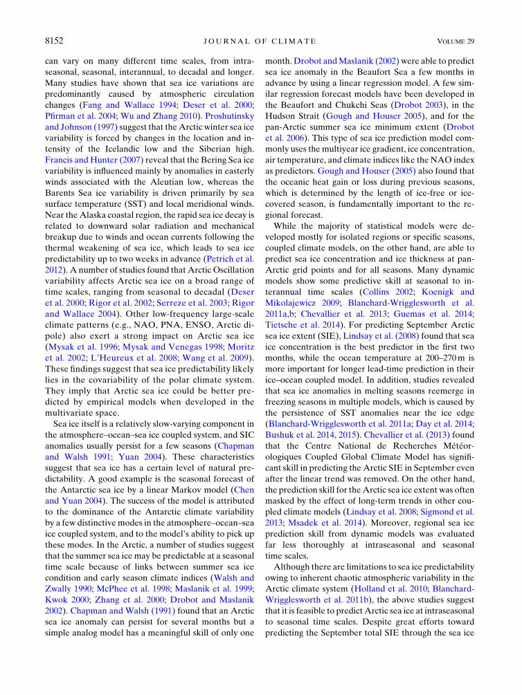
FIG. 1. (a) Linear trends and (b) standard deviation of Arctic sea ice concentration monthly mean anomalies

for the period from 1979 to 2012. Six areas that have large standard deviations are selected to assess prediction

skill of the linear Markov model. Marked with black boxes in (b), these six areas are in the Baffin Bay (Baf),

Barents Sea (Bar), East Siberian Sea (ES), eastern Chukchi Sea (Chu), Bering Sea (Ber), and Sea of Okhotsk

(Okh).

15 NOVEMBER 2016 YUAN ET AL . 8155

exceeds the SIC anomaly persistence in terms of AC

and drastically reduces RMSE from the anomaly per-

sistence, regardless of what variables are included.

Second, prediction skill is highly variable throughout

the Arctic. The skill is quite high in the Chukchi Sea,

above 0.6 even at a 12-month lead. It is followed by the

skill in the East Siberian Sea, Barents Sea and Baffin

Bay. The skill in the Sea of Okhotsk and Bering Sea is

relatively low. Third, different regions need different

combinations of model variables. For AC calculation

with a sample size of 396 for any given lead time, the 0.1

difference between two ACs (both .0.5) would be

significant at the 95% confidence level, based on a two-

tailed Fisher r-to-z transformation. The model built on

the data matrix of SIC, SAT, and SST performs better

in most areas except in the Chukchi Sea and Bering

Sea, where geopotential height and winds contribute

most to the skill in 1- to 4-month-lead predictions. It

reflects that dynamic processes are more important

than the thermodynamic process to the short-term

SIC predictability in these regions. On the other

hand, the thermodynamic process dominates the

model skill in lead times longer than four months in

the Chukchi Sea. The RMSE show similar charac-

teristics revealed by AC. It is worth mentioning

that the skill in the Arctic peripheral seas mainly re-

flects the model performance in winter and spring,

while the skill in marginal seas within the Arctic basin

reflects the skill in summer and fall in Figs. 4 and 5.

The seasonally averaged skill is quite close to the

annually averaged skill since zero anomaly data

points (such as summer SIC in the Bering Sea and

FIG. 2. Eigenvectors of the first threeMEOFmodes of (left to right) Arctic SIC, SST, SAT, and 300-hPa geopotential height and winds.

The SIC anomaly is shown as a percentage and the units for SST, SAT, and geopotential height anomalies are 8C, 8C, and 10m, re-

spectively. The maximum wind vector in (d),(h), and (l) is 5m s21. Percentages of variance explained by (top to bottom) the three modes

are 11%, 6%, and 4%.

8156 JOURNAL OF CL IMATE VOLUME 29

winter SIC in the Chukchi Sea) do not contribute

much to the correlation.

Since surface temperatures seem to contributemost to

the model skill, we ran another set of experiments to

isolate the contributions from SST and SAT. SST clearly

plays a more important role than SAT (not shown).

Including both SST and SAT slightly outperforms the

case without SAT; thus, SAT is a minor contributor but

can still contribute to the skill. Since most areas and lead

times we tested show that the combination of SIC, SST,

and SAT produces better prediction skill (Figs. 4 and 5),

we decide to use these three variables to construct

the model.

Although sea ice concentration is observable from

space, it alone does not reflect all sea ice dynamic be-

havior. We also conducted model experiments that in-

clude sea ice thickness (SIT). The ice thickness data

were taken from a pan-Arctic ice ocean modeling and

assimilation system (PIOMAS; Zhang and Rothrock

2003). The Markov model quickly gains skill when it

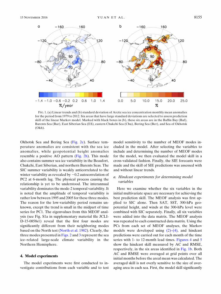
includes SIT in the Barents, East Siberian, and Chukchi

Seas (Figs. 6b–d). Including atmospheric variables and

SST only slightly enhances skill there. In the Baffin

Bay, ice thickness dominates the prediction skill for all

lead months. Adding atmosphere variables and SST

only reduces the skill (Fig. 6a). Surprisingly, adding sea

ice thickness to the model has a negative contribution

to the prediction skill in the Bering Sea and the Sea of

Okhotsk (Figs. 6e,f). Why ice thickness reduces pre-

diction skill in these regions remains unknown. One

possible reason is that PIOMAS ice thickness has

larger errors in the Bering Sea and the Sea of Okhotsk.

TheMarkov model skill is likely sensitive to the quality

of ice thickness data. This hypothesis is difficult to

verify owing to the lack of observations to evaluate ice

thickness in PIOMAS and other oceanic reanalysis

products (Chevallier et al. 2016), particularly in the

Bering Sea and the Sea of Okhotsk. On the other hand,

by using the oceanic and atmospheric variables pre-

sented here, the model captures the majority of pre-

dictable variance without having access to the ice

thickness information. It reflects the effectiveness of

building a Markov model in the MEOF space. There-

fore, we do not rely on ice thickness derived from

PIOMAS in our model development.

It is worth mentioning two SIC characteristics pre-

sented in the persistence prediction. First, both persis-

tence prediction skill and persistence RMSE in Figs. 4

and 5 show low predictability and large errors at

around a 6-month lead time. It reflects the fact that

summer SIC anomalies in the Arctic basin cannot pre-

dict winter ice condition by the persistence model be-

cause of low SIC variability due to the total freeze-up in

winter. Similarly, winter SIC anomalies in the Arctic

peripheral seas will not lead to a correct prediction in

summer by the persistence model owing to complete sea

ice melt in summer. In such a case, the persistence and

damped persistence models are worse than climatology

predictions (Fig. 5). On the other hand, the Markov

model does not have such shortcomings at the 6-month-

lead prediction. Second, the skill of the SIC persistence

in some locations increases after reaching its minimum

(see Figs. 4 and 6), reflecting the reemergence of SIC

anomalies suggested in early studies (Blanchard-

Wrigglesworth et al. 2011a; Day et al. 2014; Bushuk et al.

2014, 2015). The reemergence of SIC anomalies occurs

at 6-month (the SIC anomaly in the melting season re-

appears during the freezing season) and year-to-year

time scales. Since the SIC persistence presented here is

averaged from all seasons, the 6-month reemergence is

smoothed out but the annual reemergence stands out

clearly. This reemergence characteristic partially con-

tributes to the long-lead predictability of SIC anomalies.

b. Cross-validated experiments for determiningmodel truncation

Eigenvalues of theMEOF analysis with SIC, SST, and

SAT also suggest that only the first four MEOF modes

FIG. 3. Principal components of (top to bottom) the first-, second-,

and third-MEOF modes of Arctic SIC, SST, SAT, and 300-hPa

geopotential height and winds, from 1979 to 2013.

15 NOVEMBER 2016 YUAN ET AL . 8157

are well separated from their neighboring modes

(Fig. S1b in supplementary material file JCLI-D-15-

0858s1). The question is whether these four modes

capture most predictable variability in the pan-Arctic

region. To determine a reasonable model truncation, we

run cross-validated experiments with the model retain-

ing 1 to 13 modes, respectively. The experiments are

repeated over 34 years for a robust assessment as de-

scribed in the section 2. The demand on the number of

modes in the Markov model varies greatly across the

Arctic (Figs. S2 and S3), so we decide to choose a con-

figuration that better fits most areas and seasons.

Therefore, the model skill is evaluated using the fol-

lowing three globally averaged measures. First, we

calculated the mean AC for all grid points that have

significant correlations. Second, we calculated the

percentage of grid points that have significant corre-

lations in the latitude band of 508–808N for winter and

spring, and 758–908N for summer and fall. The purpose

is not to compare the differences between winter and

FIG. 4. Hindcast skill measured by AC between predictions and observations averaged in the (a) Baffin Bay,

(b) Barents Sea, (c) East Siberian Sea, (d) Chukchi Sea, (e) Bering Sea, and (f) Sea of Okhotsk, as a function of the

number of lead months and the variables included: SIC alone (red), plus SST and SAT (blue), plus 300mb geo-

potential height (cyan), plus 300mb wind (green), and all (black). Black dashed lines indicate the anomaly per-

sistence, which is calculated by the AC of the observed SIC anomaly series in each area. Locations of these seas are

marked in Fig. 1. We included 11 MEOF in the model for these experiments.

8158 JOURNAL OF CL IMATE VOLUME 29

summer but to identify skill differences induced by

retaining different number of modes within these sea-

sons. Third, we compute the mean RMSE in the areas

where ACs are significant. These evaluations focused

on the areas that exhibit significant sea ice pre-

dictability. We consider that the model is overfitted

when theAC remains the same (or reduced) but RMSE

is increased. The model with 1 to 5 modes clearly has

lower skill than that with 7 to 13 modes in all seasons

(Figs. 7a,b). In summer and fall, the model with one to

five modes also has a relatively low percentage of sig-

nificant correlation and higher RMSE (Figs. 7c,e). To

our surprise, the model with one to five modes has a

higher percentage of grid points with significant cor-

relation and lower RMSE in winter and spring, al-

though skill is lower (Figs. 7b,d,f). On the other hand,

the mean skill of the model experiments with 7 to 13

modes is quite similar, in which the model with 11 and

13 modes has slightly better skill and higher percentage

of significant correlations up to a 4-month lead time as

well as lower RMSE in summer and fall. However, the

model with 13 modes shows a clear lower percentage of

significant correlation and higher RMSE in winter and

spring (Figs. 7d,f). It indicates that including 13 modes

does not bring more predictability but likely introduces

more unpredictable noise. To avoid overfitting the

FIG. 5. As in Fig. 4, but for RMSE. TheRMSE from the damped anomaly persistence and climatology predictions

are also included. Here, the black broken lines mean persistence (only dashes), damped persistence (dotted), and

climatology (dot–dashed).

15 NOVEMBER 2016 YUAN ET AL . 8159

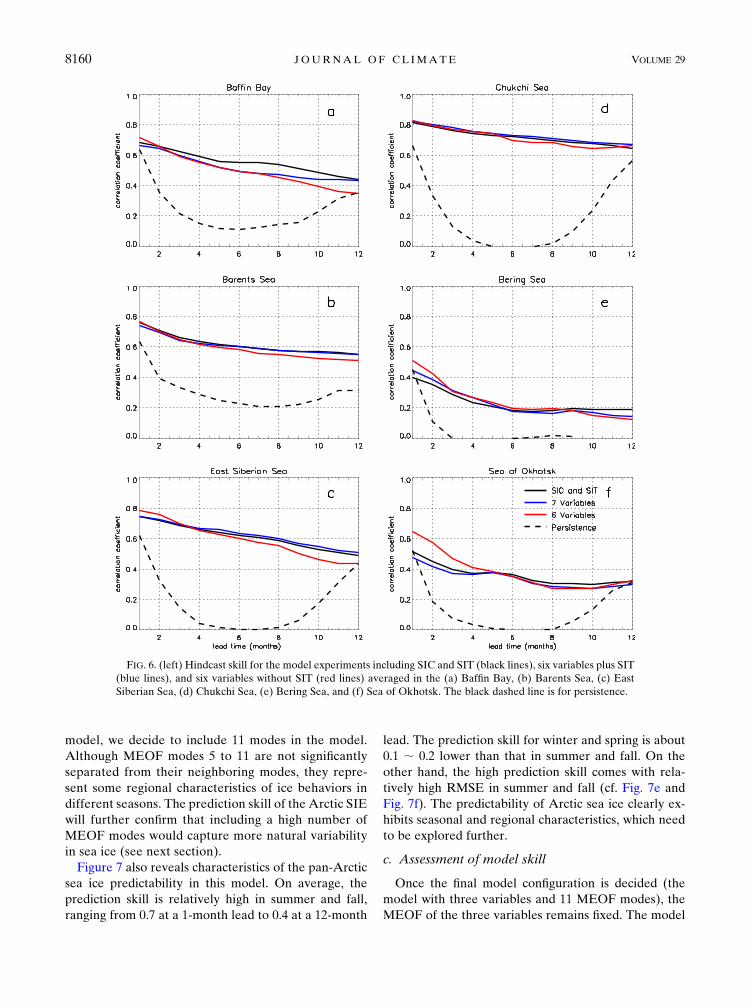
model, we decide to include 11 modes in the model.

Although MEOF modes 5 to 11 are not significantly

separated from their neighboring modes, they repre-

sent some regional characteristics of ice behaviors in

different seasons. The prediction skill of the Arctic SIE

will further confirm that including a high number of

MEOF modes would capture more natural variability

in sea ice (see next section).

Figure 7 also reveals characteristics of the pan-Arctic

sea ice predictability in this model. On average, the

prediction skill is relatively high in summer and fall,

ranging from 0.7 at a 1-month lead to 0.4 at a 12-month

lead. The prediction skill for winter and spring is about

0.1 ; 0.2 lower than that in summer and fall. On the

other hand, the high prediction skill comes with rela-

tively high RMSE in summer and fall (cf. Fig. 7e and

Fig. 7f). The predictability of Arctic sea ice clearly ex-

hibits seasonal and regional characteristics, which need

to be explored further.

c. Assessment of model skill

Once the final model configuration is decided (the

model with three variables and 11 MEOF modes), the

MEOF of the three variables remains fixed. The model

FIG. 6. (left) Hindcast skill for the model experiments including SIC and SIT (black lines), six variables plus SIT

(blue lines), and six variables without SIT (red lines) averaged in the (a) Baffin Bay, (b) Barents Sea, (c) East

Siberian Sea, (d) Chukchi Sea, (e) Bering Sea, and (f) Sea of Okhotsk. The black dashed line is for persistence.

8160 JOURNAL OF CL IMATE VOLUME 29

prediction skill was evaluated at all grid points and for

all seasons in the cross-validated fashion for the 34-yr

period. For winter (DJF) prediction, high skill is con-

centrated in the Atlantic sector of the Arctic marginal

seas and thier peripheral seas: the Barents Sea, Kara

Sea, Baffin Bay, and Labrador Sea. The skill is only

slightly reduced from a 3-month to 9-month lead. The

Sea of Okhotsk and the Bering Sea have relatively low

prediction skill. This is likely because dominant coupled

climate variability occurs in the Atlantic sector and

covariability with smaller amplitudes unique to the Pa-

cific sector is not picked up by the leading modes.

Moreover, the geopotential height and wind information

that contribute to the model skill in the Bering Sea

were not included in the model. The skill in the central

Arctic basin is also low because the area is nearly 100%

covered by sea ice in winter (Fig. 8). Prediction skill

in spring has a similar pattern to that in winter but

with lower predictability. In summer (JJA), sea ice

in the Arctic peripheral seas is melted. All prediction

skill is concentrated within theArctic basin: the 3-month-

lead prediction has skill above 0.6 for most of the central

basin. Reduced skill is found near the marginal seas,

particularly for the longer lead time. The prediction skill in

fall has a similar spatial pattern as that in summer but

with higher skill, particularly for 9-month-lead predictions.

FIG. 7. (a),(b) Mean skill; (c),(d) percentages of grid points that have significant correlation; and (e),(f) mean

RMSE: for (left) summer and fall and (right) winter and spring for number of modes 1 (dashed green), 3 (dashed

blue), 5 (dashed red), 7 (solid green), 9 (solid blue), 11 (solid red), and 13 (solid black).

15 NOVEMBER 2016 YUAN ET AL . 8161

FIG. 8. Cross-validatedmodel skill measured byACs betweenmodel predictions and observations of Arctic SIC anomalies as a function

of (top to bottom) seasons and (left to right) the number of month lead times. Only the correlations that are significant at the 95%

confidence level based on a Student’s t test are included in the panels.

8162 JOURNAL OF CL IMATE VOLUME 29

This could be related to the Arctic sea ice anomaly re-

emergence from spring to fall due to the oceanic memory

(Blanchard-Wrigglesworth et al. 2011a; Bushuk et al.

2014, 2015). In general, the model has higher prediction

skill for summer and fall than for winter and spring, while

skill is the lowest in spring.

In contrast to the higher ACs in the Atlantic sector

than the Pacific sector, the RMSEs are more uniformly

distributed around the Arctic, slightly higher in the

Barents Sea and Bering Sea in winter and spring (cf.

Fig. 8 to Fig. 9). Themagnitudes of the RMSE stay at the

same level from a 3-month to 9-month lead. The pattern

and magnitudes of RMSE for summer and fall pre-

dictions are also quite similar, although the marginal

seas have relatively larger errors than the central basin

(Fig. 9). Occasionally, RMSE can reach above 25% of

the ice concentration, which is a quite substantial error.

However, RMSE is consistently smaller than the stan-

dard deviation of ice concentration anomalies across the

Arctic (Fig. S4 in supplementary material file JCLI-D-

15-0858s1).

In addition, the model performance is further evalu-

ated against threemetrics: anomaly persistence, damped

anomaly persistence, and climatology. The damped

anomaly persistence and anomaly persistence behave

similarly in terms of AC but produce different RMSE

(Wang et al. 2016). So we evaluate the model prediction

against these metrics through RMSE. Averaged over

pan-Arctic grid points and over 34-yr model experi-

ments, the mean RMSE of Markov model predictions

of SIC does not change much with lead time but is

consistently smaller than that produced by anomaly

persistence, damped anomaly persistence, and clima-

tology predictions for all four seasons (Fig. 10). The

model’s mean RMSE is larger in summer and fall than

in winter and spring, reflecting larger SIC variability in

summer and fall. Even though the mean RMSEs from

Markov model predictions are only slightly smaller

than climatology predictions in spring (Fig. 10), the

differences between these two sets of RMSEs are sta-

tistically significant owing to the large sample size

(357 390).

To assess the performance of the Markov model rel-

ative to dynamic forecast systems, we calculated the skill

from the NCEP Climate Forecast System, version 2

(CFSv2; Wang et al. 2013), which has similar perfor-

mance compared to other dynamic forecast systems

(Merryfield et al. 2013; Blanchard-Wrigglesworth et al.

2015). The Markov model appears superior in most

areas that we examined in terms of prediction skill

(Fig. 11). The skill of these two models is comparable

only in the Sea of Okhotsk. It is worth mentioning that

the hindcast skill in this statistical model is not

calculated in the same way as the hindcast skill in the

dynamic model. However, they are the available metrics

for comparisons between different types of models. The

model also shows an advantage over earlier statistical

models, such as the analogmodel presented in Chapman

andWalsh (1991), which cannot outperform persistence

beyond a 1-month lead.

d. Prediction of Arctic sea ice extent

The Arctic SIE forecast in all months is calculated by

summing all areas that have at least 15% sea ice con-

centration from the SIC predictions produced by cross-

validated experiments and from observations. Here we

use September SIE forecast to illustrate themodel’s skill

in predicting Arctic SIE. Figure 12 shows the 2-, 3-, and

4-month-lead September SIE predictions during 1980 to

2012 and the forward forecasts in 2013 and 2014. The

model generally predicts the phase of SIE variability

well but with weaker amplitudes of variability. It was

able to predict the historical low in 2007 and 2012 and

also captured the bounce back in 2013 and 2014 in the

forward forecast (Figs. 12a–c). However, it did not

capture the accelerated SIE decline, particularly in the

last decade. The model skill of predicting September

SIE measured by ACs and RMSE is listed in Table 1.

These model assessments reflect its ability to predict

anomaly phases (high AC) and its deficiency in accu-

rately predicting magnitudes of anomalies. The model

systematically overestimates the September SIE. One

possible reason for this model behavior is that themodel

is developed in the multivariate space. Sea ice likely has

the strongest trend among all oceanic and atmospheric

variables. The trends in PCs of MEOF modes may not

present the true strength of sea ice trends. To overcome

this model deficiency, we consider two types of model

bias corrections for SIE predictions.

The first-order or mean bias correction method can be

achieved by subtracting a mean prediction error during

1980–2012 from all predictions. The bias correction re-

duces overestimation of SIE in the recent decade but

produces underestimation of SIE in early years. This

method does not change the model correlation skill but

reduces approximately 30%ofRMSE for all predictions at

2- to 4-month lead times. (Table 1).

The second approach of bias correction is to predict

model errors. The forecast errors display a relatively

good linear relationship with SIE anomalies in the initial

months for 2- and 3-month-lead forecasts, although

such a relationship vanishes in the 4-month-lead forecast

(Figs. 12d–f). This indicates that SIE has limited dura-

tion of memory. The linear relationship allows us to

conduct a bias correction using linear regression for the

short-term predictions:

15 NOVEMBER 2016 YUAN ET AL . 8163

FIG. 9. RMSE averaged over 34 yr of cross-validated experiments as functions of (top to bottom) seasons and (left to right) the number

of month lead times.

8164 JOURNAL OF CL IMATE VOLUME 29

SIEb(t, n)5a3 SIE

a(t2 n)1b , (5)

where SIEb represents the n-month-lead forecast bias

(error) at the tth month and is expressed as the linear

regression of the SIE anomaly SIEa at the (t 2 n)th

month. The slope of the regression a represents the

linear dependence on SIEa and the intercept b, the

constant bias at zero anomaly. Such a bias correction

does not use information beyond the lead time and is

thus a forecast method for the SIE residual that has not

been resolved by the linear Markov model for SIC. This

method is most effective for the 2-month-lead forecast,

which shows both enhanced correlations and reduced

RMSE (Fig. 12 and Table 1). Specifically, the method

reduces 62% of RMSE from the prediction without bias

correction and removes an additional 41% of RMSE

from the prediction with the constant bias correction.

The skill for the 3-month-lead prediction was improved

slightly from the results of prediction by constant bias

correction. However, it does not show much improve-

ment from the prediction with constant bias corrections

for 4-month-lead predictions (Table 1). Because of a

very low value of a (0.02) for the 4-month-lead pre-

diction, the linear regression bias correction is equivalent

to the constant bias correction. Both bias corrections

improve model predictions mainly through reducing the

model’s RMSE.

This linear regression bias correction is different than

the methods presented in Kharin et al. (2012) and

Fu�ckar et al. (2014). In Kharin et al. (2012), both pre-

dictions and observations can be expressed separately

by a linear trend plus anomalies relative to the linear

trend. The linear regression bias correction is then

achieved by replacing the linear trend in predictions

with the linear trend in observations. In Fu�ckar et al.

(2014), predictions and observations were expressed

separately by linear regressions of observed initial con-

ditions plus anomalies with respect to the linear re-

gressions. The regression bias correction is then

achieved by replacing the linear regression in the model

forecast with the linear regression in observations. For

SIE prediction, these three types of linear regression

bias correction produce similar results (Wang

et al. 2016).

e. Contribution of linear trends to the prediction skill

In general, there are two types of predictability in a

climate system: one is forced or derived from changing

FIG. 10. The mean RMSE of Markov model predictions (solid black) compared against the mean RMSE of

anomaly persistence (dotted), damped anomaly persistence (dashed), and climatology (dashed–dotted) predictions

as function of seasons and the number of month lead times . The pan-Arctic average is carried out on the grid points

where observed SIC variability (standard deviation) is .10%.

15 NOVEMBER 2016 YUAN ET AL . 8165

boundary conditions; another comes from initial condi-

tions or internal variability (Lorenz 1975). In the Arctic,

we consider that the long-term trend is forced by the

climate change. Because of the rapid decline of Arctic

sea ice, linear trends in sea ice account for a large por-

tion of prediction skill in dynamic models (Lindsay et al.

2008; Blanchard-Wrigglesworth 2011b; Sigmond et al.

2013; Msadek et al. 2014). To isolate the contribution of

sea ice trends to the prediction skill in the linearMarkov

model, we conducted postprediction analysis on the

predictions from cross-validated experiments. Monthly

trends at each grid point were removed from the pre-

dictions and observations. The skill of detrended pre-

diction is evaluated by ACs of the residual series. On

average, the trend removal reduces the skill by 0.16

(0.25) of AC for the 3-month (6 month) lead predictions

and leaves 9-month predictions without any skill for all

seasons (Fig. 13). Large skill reduction occurs north of

the Chukchi Sea as well as in the East Siberian Sea and

the Barents–Kara Seas, where SIC has large declining

FIG. 11.Mean hindcast skill (AC) of the linearMarkovmodel (solid black) and CFSv2 (dashed black) as function

of the number of month lead times in the (a) Baffin Bay, (b) Barents Sea, (c) East Siberian Sea, (d) Chukchi Sea,

(e) Bering Sea, and (f) the Sea of Okhotsk. See Fig. 1b for the locations of these seas. The sea ice anomaly per-

sistence (black dotted lines) is the benchmark for the skill.

8166 JOURNAL OF CL IMATE VOLUME 29

FIG. 12. The (a) 2-, (b) 3-, and (c) 4-month-lead predictions of the September SIE without (dotted lines) and with

(dashed lines) regression bias corrections compared with observations (solid). Crosses (circles) are forward pre-

diction of September SIE in 2013 and 2014 without (with) regression bias correction. Scatterplots of the (d) 2-,

(e) 3-, and (f) 4-month-lead forecast errors of September SIE as a function of initial month SIE anomalies. The solid

line represents the linear fit of the data, and the dashed (dotted) curves show the 95% confidence interval of the fit

(predicted bias).

15 NOVEMBER 2016 YUAN ET AL . 8167

trends (Fig. 1a). However, the model still retains the

predictive skill (AC . 0.6) in the central Arctic for

3-month-lead summer and fall predictions and in the

Canadian basin for 6-month-lead fall predictions

(Fig. 13). In winter and spring, the peripheral seas in the

Atlantic sector also lose predictive skill after the trend

removal (cf. Fig. 8 and Fig. 13) but retain predictive skill

for 2-month-lead winter prediction (not shown). Al-

though the trend removal largely reduces SIC pre-

diction skill, the residual skill still beats the detrended

persistence prediction in most areas in the Arctic basin

for summer (fall) predictions up to 6-month (9 month)

lead time, as well as in Arctic peripheral seas for

3-month-lead winter and spring predictions (Fig. S5 in

supplementary material file JCLI-D-15-0858s1). This

means that the model captures certain SIC internal

variability.

Furthermore, we examine the trend’s contribution to

the prediction skill of Arctic SIE. The model has skillful

predictions of Arctic SIE fromNovember to January for

most lead times and high skill predictions from July to

September up to 8-month lead times (Fig. 14a). Then we

remove the monthly trends from SIE predictions and

observations. As shown in section 4d, theMarkovmodel

underestimates the strength of the linear trend in

September SIE. The model behaves similarly in other

months. Removal of monthly linear trends in-

dependently from the predictions and observations ac-

tually improves the prediction skill for all seasons, which

shows the ability of the model in predicting year-to-year

variability of Arctic SIE. After the trend removal, the

model is skillful (AC . 0.6) in predicting SIE from

September to February but has low predictability from

March to June (Figs. 14a,b). The improvements are es-

pecially large in June and October because the model

produces larger errors in predicting the trends in these

two months. Before the trend removal, the model’s SIE

prediction can only beat anomaly persistence in isolated

months with limited lead times (Fig. 14c). After the

trend removal, the model can beat the persistence in

most months and most lead times (Fig. 14d). The SIE

forecast by the Markov model has smaller RMSEs than

that by climatology prediction, except for spring fore-

casts with trends or without trends (Fig. S7 in supple-

mentary material file JCLI-D-15-0858s1). Compared to

the Canadian seasonal and interannual prediction sys-

tem (Fig. 2 in Sigmond et al. 2013), the Markov model is

more capable of capturing natural variability during all

seasons but is less capable of correctly predicting long-

term trends in SIE.

On the other hand, if the Markov model only retains

four independent MEOF modes (Fig. S1b), the model

loses overall prediction skill in winter (cf. Fig. 14a and

Fig. S5a) and loses a significant amount of skill in pre-

dicting internal variability in spring at 1- to 3-month

lead time (cf. Fig. 14b and Fig. S6b). It confirms that

retaining more modes in the model helps capture more

internal variability and trends’ contribution in SIE

predictions.

5. Summary and discussion

In this study, we developed a reduced-dimension

stochastic model—namely, a linear Markov model—to

predict Arctic SIC at the seasonal time scale. The model

is constructed in the multivariate (MEOF) space with

variables from the atmosphere, ocean, and ice field so

that it captures the covariability of the Arctic climate

system. Because of the complexity of Arctic geography

and regional–seasonal characteristics of atmosphere–

ocean–sea ice interaction, the determinants of the

model’s variables and its number of MEOF modes are

not unique. However, the differences in prediction skill

from using different numbers of variables and MEOF

modes are relatively small compared to the Markov

model for Antarctic sea ice (Chen and Yuan 2004).

Based on a trial-and-error method, we chose 3 variables

(SIC, SST, and SAT) with 11 MEOF modes as the final

model configuration, which was used in this study to

assess model performance and make forward forecast.

The results from 3 variables and 11 modes are similar to

the results derived from 6 variables and 11 modes. The

final choice of model configuration better fits the sum-

mer and fall prediction but may be overfitting for winter

and spring prediction.

The linear Markov model shows good skill in pre-

dicting signs of Arctic sea ice concentration anomaly a

few seasons in advance. The predictability strongly de-

pends on seasons and locations and is especially high

within the Arctic basin during summer and fall. The

model AC stays above 0.6 even at a 9-month lead

for these seasons in the Chukchi, Beaufort, Eastern

TABLE 1. The skill (r) and RMSE of September Arctic SIE

predictions based onMarkovmodel SIC predictionwith 3 variables

and 11 modes as a function of the number of lead months All

correlations (r values) are significant at the 99% confidence level.

Prediction

without bias

correction

Prediction

with constant

bias

correction

Prediction

with re-

gression bias

correction

Lead month r RMSE r RMSE r RMSE

2 0.82 0.95 0.82 0.73 0.92 0.41

3 0.73 1.07 0.73 0.82 0.77 0.74

4 0.78 1.03 0.78 0.80 0.78 0.78

8168 JOURNAL OF CL IMATE VOLUME 29

FIG. 13. The model skill measured by AC between detrended predictions and detrended observations. Only the correlations that are

significant at the 95% confidence level based on a Student’s t test are included: (top to bottom) seasons and (left to right) number of

months lead times.

15 NOVEMBER 2016 YUAN ET AL . 8169

Siberian, Kara, and Barents Seas. The winter skill is 0.5

for up to 9-month-lead forecasts in the marginal and

peripheral seas of the Arctic, such as the Barents Sea,

Greenland Sea, and Baffin Bay. The pattern of pre-

diction skill in spring is very similar to that in winter but

with lower correlations. In general, the forecast skill is

better in the Atlantic sector of the Arctic than in the

Pacific sector and better in summer and fall than in

winter and spring. The lowest prediction skill occurs in

the Bering Sea. On the pan-Arctic average, the model’s

skill is superior to the skill derived from anomaly per-

sistence, damped anomaly persistence, and climatology

predictions. The long-term trends in the Markov model

predictions contribute largely to the SIC summer and

fall forecast skill in the Chukchi, East Siberian, and

Barents Seas as well as winter forecast skill in the pe-

ripheral seas of the Atlantic sector. However, the model

retains skillful 3-month-lead summer and fall pre-

dictions in the central Arctic and 6-month-lead fall

predictions in the Canadian basin after the trends were

removed. Moreover, the model’s skill is consistently

higher than the persistence skill after all trends were

removed from summer and fall predictions, revealing

the model’s ability to capture some predictable SIC in-

ternal variability. The success of the model is attributed

to the dominance of several distinct modes in the cou-

pled atmosphere–ocean–sea ice system and to the

model’s ability to pick up these modes. However, the

relationships between sea ice and the ocean as well as

atmosphere likely vary in different climate regimes

(Holland and Stroeve 2011). A statistical model would

not be at its best performance for a long period, partic-

ularly for the rapidly declining arctic sea ice. Periodi-

cally retraining the Markov model is needed to keep its

skill updated.

In addition, the SIE prediction can be derived from

predicted SIC. Our results show that SIE is most pre-

dictable in September and in winter and least predict-

able in spring (Fig. 14). Contrasting to the trend’s

contribution to SIC prediction skill, the calculated SIE

predictions cannot capture the rapid decline trends in

observed SIE but are able to capture the internal vari-

ability. Removing monthly trends from SIE prediction

improves its prediction skill. The SIE predictions with-

out linear trends are superior to the detrended persis-

tence for most months and lead times. Moreover, the

SIE prediction by the Markov model consistently out-

performs the climatology prediction in terms of RMSE

except in spring, regardless of whether one considers

trends. It demonstrates that the model predicts Arctic

SIE’s internal variability better than its long-term

trends. Predicting September SIE is given as an exam-

ple to illustrate the model’s forecast skill for SIE. Al-

though the model has a relatively high skill in predicting

the Arctic SIE, it systematically overestimates the

September SIE. This model bias can be corrected by two

FIG. 14. Cross-validated prediction skill (AC) for the Arctic SIE by the Markov model with 3 variables and 11

modes using (a) original time series and (b) detrended prediction skill. The x axis represents target month and the y

axis represents the number of lead months. Black 3 symbols mark correlations that are significant at the 95%

confidence level by the Student’s t test. (c) The AC differences between the model SIE prediction and persistence

prediction. Positive values indicate that the model is superior to the persistence. (d) As in (c), but for detrended

predictions and detrended persistence.

8170 JOURNAL OF CL IMATE VOLUME 29

methods: a constant bias correction by removing the

mean bias over the last 34 yr and a linear regression bias

correction by fitting model errors as a linear function of

initial SIE anomalies and then removing the regressed

errors. The regression bias correction can significantly

improve the skill of 2-month-lead forecasts and provide

better prediction than the constant bias correction (Table 1

and Fig. 12). Because theMarkovmodel for SIC is built in

the multivariate space, it might underestimate the SIE

trend since sea ice likely has the fastest declining trend in

the system. The regression bias correction can rectify the

trend quite well at 2-month lead time. On the other hand,

the 4-month-lead forecast cannot benefit from the re-

gression bias correction since prediction errors have a

near-zero slope in the regression (Fig. 12).

This study shows that the SIC within the Arctic basin

can be predicted seasons in advance by a reduced-

dimension statistical model with reasonable skill. The

Markov model effectively utilizes the linear relation-

ships between SIC and oceanic and atmospheric vari-

ability. Future improvement of the Arctic sea ice

prediction by statistical models likely relies on the ex-

ploration of the nonlinear component existing in the

Arctic climate system, or non-Markovian processes, as

well as on more sophisticated bias corrections than we

presented in this study. Moreover, the low prediction

skill in the Pacific sector of the Arctic may not be im-

proved in a pan-Arctic model. One of reasons could be

that the dominant climate variability in the northern

mid–high latitudes occurs mostly in the Atlantic sector

of theArctic and subarctic, which dictates leadingMEOF

modes. The unique characteristics of atmosphere–ocean–

sea ice coupled relationships in the Pacific sector may not

be included in the leading MEOF decompositions of the

pan-Arctic climate system and thus are not correctly

represented in the model. On the other hand, the Pacific

sector of the Arctic may need a different set of variables

to maximize the model’s predictability. A separate study

shows that the sea ice prediction in theBering Sea and the

Sea of Okhotsk can be significantly improved in a re-

gional linearMarkovmodel that focuses on the important

coupled atmosphere–ocean–sea ice relationships in these

regions (Li et al. 2016).

Acknowledgments. We gratefully acknowledge sup-

port from the Office of Naval Research Grant N00014-

12-1-0911. Anonymous reviewers’ comments helped us

greatly improve the quality of the study.

REFERENCES

Blanchard-Wrigglesworth, E., K. C. Armour, C. M. Bitz, and

E. DeWeaver, 2011a: Persistence and inherent predictability

of Arctic sea ice in a GCM ensemble and observations.

J. Climate, 24, 231–250, doi:10.1175/2010JCLI3775.1.

——, C. M. Bitz, and M. M. Holland, 2011b: Influence of initial

conditions and climate forcing on predicting Arctic sea ice.

Geophys. Res. Lett., 38, L18503, doi:10.1029/2011GL048807.

——,R. Cullather,W.Wang, J. Zhang, andC.M. Bitz, 2015:Model

forecast skill and sensitivity to initial conditions in the seasonal

sea ice outlook. Geophys. Res. Lett., 42, 8042–8048,

doi:10.1002/2015GL065860.

Blumenthal, M. B., 1991: Predictability of a coupled ocean–

atmosphere model. J. Climate, 4, 766–784, doi:10.1175/

1520-0442(1991)004,0766:POACOM.2.0.CO;2.

Bushuk, M., D. Giannakis, and A. J. Majda, 2014: Reemergence

mechanisms for North Pacific sea ice revealed through non-

linear Laplacian spectral analysis. J. Climate, 27, 6265–6287,

doi:10.1175/JCLI-D-13-00256.1.

——,——, and——, 2015: Arctic sea ice reemergence: The role of

large-scale oceanic and atmospheric variability. J. Climate, 15,

2648–2663, doi:10.1175/JCLI-D-14-00354.1.

Canizares, R., A. Kaplan, M. A. Cane, D. Chen, and S. E. Zebiak,

2001: Use of data assimilation via linear low-order models for

the initialization of El Niño–Southern Oscillation predictions.

J. Geophys. Res., 106, 30 947–30 959, doi:10.1029/

2000JC000622.

Chapman, W. L., and J. E. Walsh, 1991: Long-range prediction of

regional sea ice anomalies in theArctic.Wea. Forecasting, 6, 271–

288, doi:10.1175/1520-0434(1991)006,0271:LRPORS.2.0.CO;2.

Chen, D., and X. Yuan, 2004: A Markov model for seasonal fore-

cast of Antarctic sea ice. J. Climate, 17, 3156–3168,

doi:10.1175/1520-0442(2004)017,3156:AMMFSF.2.0.CO;2.

Chen, T. C., 2005: The structure and maintenance of stationary

waves in the winter Northern Hemisphere. J. Atmos. Sci., 62,

3637–3660, doi:10.1175/JAS3566.1.

Chevallier, M., D. Salas y Mélia, A. Voldoire, M. Deque, and

D. Garric, 2013: Seasonal forecasts of the pan-Arctic sea ice

extent using a GCM-based seasonal prediction system.

J. Climate, 26, 6092–6104, doi:10.1175/JCLI-D-12-00612.1.

——, and Coauthors, 2016: Intercomparison of the Arctic sea ice

cover in global ocean–sea ice reanalyses from the ORA-IP

project.Climate Dyn., doi:10.1007/s00382-016-2985-y, in press.

Collins, M., 2002: Climate predictability on inter-annual to de-

cadal time scales: The initial value problem. Climate Dyn.,

19, 671–692, doi:10.1007/s00382-002-0254-8.

Comiso, J. C., 2000: Bootstrap sea ice concentrations from Nimbus-7

SMMR andDMSP SSM/I-SSMIS, version 2. National Snow and

Ice Data Center Distributed Active Archive Center, updated

2015, accessed 11 October 2016, doi:10.5067/J6JQLS9EJ5HU.

Day, J. J., S. Tietsche, and E. Hawkins, 2014: Pan-Arctic and re-

gional sea ice predictability: Initialization month dependence.

J. Climate, 27, 4371–4390, doi:10.1175/JCLI-D-13-00614.1.

Deser, C., J. E. Walsh, and M. S. Timlim, 2000: Arctic sea ice vari-

ability in the context of recent atmospheric circulation trends.

J. Climate, 13, 617–633, doi:10.1175/1520-0442(2000)013,0617:

ASIVIT.2.0.CO;2.

Drobot, S., 2003: Long-range statistical forecasting of ice severity in

the Beaufort–Chukchi Sea. Wea. Forecasting, 18, 1161–1176,

doi:10.1175/1520-0434(2003)018,1161:LSFOIS.2.0.CO;2.

——, and J. A. Maslanik, 2002: A practical method for long-range

forecasting of ice severity in the Beaufort Sea. Geophys. Res.

Lett., 29, 1213, doi:10.1029/2001GL014173.

——, ——, and C. Fowler, 2006: A long-range forecast of Arctic

summer sea-ice minimum extent. Geophys. Res. Lett., 33,

L10501, doi:10.1029/2006GL026216.

15 NOVEMBER 2016 YUAN ET AL . 8171

Eicken, H., 2013: Arctic sea ice needs better forecasts.Nature, 497,

431–433, doi:10.1038/497431a.

Fang, Z., and J. M. Wallace, 1994: Arctic sea ice variability on a

timescale of weeks and its relation to atmospheric forcing.

J. Climate, 7, 1897–1913, doi:10.1175/1520-0442(1994)007,1897:

ASIVOA.2.0.CO;2.

Francis, J. A., and E. Hunter, 2007: Drivers of declining sea ice in

theArctic winter.Geophys. Res. Lett., 34, L17503, doi:10.1029/

2007GL030995.

Fu�ckar, M. S., D. Volpi, V. Guemas, and F. J. Doblas-Reyes,

2014: A posteriori adjustment of near-term climate pre-

dictions: Accounting for the drift dependence on the initial

conditions. Geophys. Res. Lett., 41, 5200–5207, doi:10.1002/

2014GL060815.

Goosse, H., O. Arzel, C. M. Bitz, A. de Montety, and

M. Vancoppenolle, 2009: Increased variability of the Arctic

summer ice extent in a warmer climate. Geophys. Res. Lett.,

36, L23702, doi:10.1029/2009GL040546.

Gough, W. A., and C. Houser, 2005: Climate memory and long-

range forecasting of sea ice conditions in Hudson Strait. Polar

Geogr., 29, 17–26, doi:10.1080/789610163.

Griffies, S. M., and K. Bryan, 1997: A predictability study of sim-

ulated North Atlantic multidecadal variability. Climate Dyn.,

13, 459–487, doi:10.1007/s003820050177.Guemas, V., and Coauthors, 2014: A review on Arctic sea-ice pre-

dictability and prediction on seasonal to decadal time-scales.

Quart. J. Roy. Meteor. Soc., 142, 546–561, doi:10.1002/qj.2401.Holland, M. M., and J. Stroeve, 2011: Changing seasonal sea ice

predictor relationships in a changing Arctic climate.Geophys.

Res. Lett., 38, L18501, doi:10.1029/2011GL049303.

——, D. A. Bailey, and S. Vavrus, 2010: Inherent sea ice pre-

dictability in the rapidly changing Arctic environment of the

Community Climate System Model, version 3. Climate Dyn.,

36, 1239–1253, doi:10.1007/s00382-010-0792-4.Kalnay, E., and Coauthors, 1996: The NCEP/NCAR 40-Year Re-

analysis Project. Bull. Amer. Meteor. Soc., 77, 437–471,

doi:10.1175/1520-0477(1996)077,0437:TNYRP.2.0.CO;2.

Kanamitsu, M., W. Ebisuzaki, J. Woollen, S.-K. Yang, J. J. Hnilo,

M. Fiorino, and G. L. Potter, 2002: NCEP–DOE AMIP-II

Reanalysis (R-2). Bull. Amer. Meteor. Soc., 83, 1631–1643,

doi:10.1175/BAMS-83-11-1631.

Kharin, V. V., G. J. Boer,W. J.Merryfield, J. F. Scinocca, andW. S.

Lee, 2012: Statistical adjustment of decadal predictions in a

changing climate.Geophys. Res. Lett., 39, L19705, doi:10.1029/

2012GL052647.

Koenigk, T., and U. Mikolajewicz, 2009: Seasonal to interannual

climate predictability in mid and high northern latitudes in a

global coupled model. Climate Dyn., 32, 783–798, doi:10.1007/

s00382-008-0419-1.

Kistler, R., and Coauthors, 2001: The NCEP–NCAR 50-Year

Reanalysis: Monthly means CD-ROM and documentation.

Bull. Amer. Meteor. Soc., 82, 247–267, doi:10.1175/

1520-0477(2001)082,0247:TNNYRM.2.3.CO;2.

Kwok, R., 2000: Recent changes in Arctic Ocean sea ice motion

associated with North Atlantic Oscillation. Geophys. Res.

Lett., 27, 775–778, doi:10.1029/1999GL002382.

L’Heureux, M. L., A. Kumar, G. D. Bell, M. S. Halpert, and R. W.

Higgins, 2008: Role of the Pacific-North American (PNA)

pattern in the 2007 Arctic sea ice decline.Geophys. Res. Lett.,

35, L20701, doi:10.1029/2008GL035205.

Lindsay, R. W., J. Zhang, A. J. Schweiger, and M. A. Steele, 2008:

Seasonal predictions of ice extent in the Arctic Ocean.

J. Geophys. Res., 113, C02023, doi:10.1029/2007JC004259.

Lorenz, E. N., 1975: The physical bases of climate and climate

modelling. Climate Predictability, WMOGlobal Atmospheric

Research Program Series, Vol. 16, World Meteorological

Organization, 132–136.

Maslanik, J. A., M. C. Serreze, and T. Agnew, 1999: On the record

reduction in 1998 western Arctic sea-ice cover.Geophys. Res.

Lett., 2, 1905–1908, doi:10.1029/1999GL900426.

McPhee, M. G., T. P. Stanton, J. H. Morison, and D. G. Martinson,

1998: Freshing of the upper ocean in the Arctic: Is perennial

sea ice disappearing? Geophys. Res. Lett., 25, 1729–1732,

doi:10.1029/98GL00933.

Merryfield, W. J., W.-S. Lee, W. Wang, M. Chen, and A. Kumar,

2013: Multi-system seasonal predictions of Arctic sea ice.

Geophys. Res. Lett., 40, 1551–1556, doi:10.1002/grl.50317.Moritz, R. E., C. M. Bitz, and E. J. Steig, 2002: Dynamics of recent

climate change in the Arctic. Science, 297, 1497–1502,

doi:10.1126/science.1076522.

Msadek,R.,G.Vecchi,M.Winton, andR.G.Gudgel, 2014: Importance

of initial conditions in seasonal predictions of Arctic sea ice extent.

Geophys. Res. Lett., 41, 5208–5215, doi:10.1002/2014GL060799.

Mysak, L.A., and S. A. Venegas, 1998: Decadal climate oscillations

in the Arctic: A new feedback loop for atmosphere-ice-ocean

interactions. Geophys. Res. Lett., 25, 3607–3610, doi:10.1029/

98GL02782.

——, R. G. Ingram, J. Wang, and A. van der Baaren, 1996: The anom-

alous sea-ice extent in Hudson Bay, Baffin Bay, and the Labrador

Sea during three simultaneous NAO and ENSO episodes.Atmos.–

Ocean, 34, 313–343, doi:10.1080/07055900.1996.9649567.

North, G. R., T. L. Bell, R. F. Cahalan, and F. J. Moeng, 1982:

Sampling errors in the estimation of empirical orthogonal

functions. Mon. Wea. Rev., 110, 699–706, doi:10.1175/

1520-0493(1982)110,0699:SEITEO.2.0.CO;2.

Parkinson, C. L., and D. J. Cavalieri, 2012: Antarctic sea ice vari-

ability and trends, 1979–2010. Cryosphere, 6, 871–880,

doi:10.5194/tc-6-871-2012.

Petrich, C., H. Eicken, J. Zhang, J. Krieger, Y. Fukamachi, andK. I.

Ohshima, 2012: Coastal landfast sea ice decay and breakup in

northern Alaska: Key processes and seasonal prediction.

J. Geophys. Res., 117, C02003, doi:10.1029/2011JC007339.

Pfirman, S., W. F. Haxby, R. Colony, and I. Rigor, 2004: Variability

in Arctic sea ice drift. Geophys. Res. Lett., 31, L16402,

doi:10.1029/2004GL020063.

Proshutinsky,A., andM. Johnson, 1997: Two circulation regimes of

the wind-driven Arctic Ocean. J. Geophys. Res., 102, 12 493–

12 514, doi:10.1029/97JC00738.

Rayner, N. A., D. E. Parker, E. B. Horton, C. K. Folland, L. V.

Alexander, D. P. Rowell, E. C. Kent, and A. Kaplan, 2003:

Global analyses of sea surface temperature, sea ice, and night

marine air temperature since the late nineteenth century.

J. Geophys. Res., 108, 4407, doi:10.1029/2002JD002670.

Rigor, I. G., and J. M. Wallace, 2004: Variation in the age of Arctic

sea-ice and summer sea-ice extent. Geophys. Res. Lett., 31,

L09401, doi:10.1029/2004GL019492.

——, ——, and R. L. Colony, 2002: Response of sea ice to the

Arctic Oscillation. J. Climate, 15, 2648–2668, doi:10.1175/

1520-0442(2002)015,2648:ROSITT.2.0.CO;2.

Serreze,M. C., and Coauthors, 2003: A record minimumArctic sea

ice extent and area in 2002. Geophys. Res. Lett., 30, 1110,

doi:10.1029/2002GL016406.

Sigmond, M., J. C. Fyfe, G. M. Flato, V. V. Kharin, and W. J.

Merryfield, 2013: Seasonal forecast skill of Arctic sea ice area

in a dynamical forecast system. Geophys. Res. Lett., 40, 529–

534, doi:10.1002/grl.50129.

8172 JOURNAL OF CL IMATE VOLUME 29

Simmonds, I., 2015: Comparing and contrasting the behavior of

Arctic and Antarctic sea ice over the 35 year period 1979–

2013. Ann. Glaciol., 56, 18–28, doi:10.3189/2015AoG69A909.

Tietsche, S., and Coauthors, 2014: Seasonal to interannual Arctic

sea ice predictability in current global climate models. Geo-

phys. Res. Lett., 41, 1035–1043, doi:10.1002/2013GL058755.

Ting, M. F., 1994: Maintenance of northern summer stationary

waves in a GCM. J. Atmos. Sci., 51, 3286–3308, doi:10.1175/1520-0469(1994)051,3286:MONSSW.2.0.CO;2.

Walsh, J. E., and H. J. Zwally, 1990: Multiyear sea ice in the

Arctic: Model- and satellite-derived. J. Geophys. Res., 95,

11 613–11 628, doi:10.1029/JC095iC07p11613.

Wang, J., J. Zhang, E. Watanabe, M. Ikeda, K. Mizobata, J. E.

Walsh, X. Bai, and B.Wu, 2009: Is the dipole anomaly a major

driver to record lows in Arctic summer sea ice extent? Geo-

phys. Res. Lett., 36, L05706, doi:10.1029/2008GL036706.

Wang,L.,X.Yuan,M.Ting, andC.Li, 2016: Predicting summerArctic

sea ice concentration variability using a vector autoregressive

model. J. Climate, 29, 1529–1543, doi:10.1175/JCLI-D-15-0313.1.

Wang,W.,M.Chen, andA.Kumar, 2013: Seasonal prediction ofArctic

sea ice extent from a coupled dynamical forecast system. Mon.

Wea. Rev., 141, 1375–1394, doi:10.1175/MWR-D-12-00057.1.

Wu, Q., and X. Zhang, 2010: Observed forcing-feedback processes

between Northern Hemisphere atmospheric circulation and

Arctic sea ice coverage. J. Geophys. Res., 115, D14119,

doi:10.1029/2009JD013574.

——, Y. Yan, and D. Chen, 2013: A linear Markov model for East

Asian monsoon seasonal forecast. J. Climate, 26, 5183–5195,doi:10.1175/JCLI-D-12-00408.1.

Xue,Y.,M.A.Cane, S.E.Zebiak, andM.B.Blumenthal, 1994:On the

prediction of ENSO: A study with a low-order Markov model.

Tellus, 46A, 512–528, doi:10.1034/j.1600-0870.1994.00013.x.

——, A. Leetmaa, and M. Ji, 2000: J. Climate, 13, 849–871,

doi:10.1175/1520-0442(2000)013,0849:EPWMMT.2.0.CO;2.

Yang, X., and X. Yuan, 2014: The early winter sea ice vari-

ability under the recent Arctic climate shift. J. Climate, 27,5092–5110, doi:10.1175/JCLI-D-13-00536.1.

Yuan, X., 2004: ENSO-related impacts on Antarctic sea ice:

Synthesis of phenomenon and mechanisms. Antarct. Sci., 16,415–425, doi:10.1017/S0954102004002238.

Zhang, J., andD.A. Rothrock, 2003:Modeling global sea ice with a

thickness and enthalpy distribution model in generalized

curvilinear coordinates. Mon. Wea. Rev., 131, 845–861,

doi:10.1175/1520-0493(2003)131,0845:MGSIWA.2.0.CO;2.

——, ——, and M. S. Steele, 2000: Recent changes in Arctic sea ice:

The interplay between ice dynamics and thermodynamics.

J. Climate, 13, 3099–3114, doi:10.1175/1520-0442(2000)013,3099:

RCIASI.2.0.CO;2.

15 NOVEMBER 2016 YUAN ET AL . 8173