ARCTAS-California 2008:An airborne mission to … 2008: An airborne mission to investigate California air quality CARB Award No. 07-335 Principal Investigator Donald R. Blake Professor,

1

Final Report

ARCTAS-California 2008: An airborne mission to investigate California air quality

CARB Award No. 07-335

Principal Investigator

Donald R. Blake

Professor, Department of Chemistry

University of California, Irvine

Irvine, CA 92697

(949) 824-4195

(949) 824-2905 (FAX)

e-mail: [email protected]

Report prepared for:

State of California Air Resources Board

Research Division

PO Box 2815

Sacramento, CA 95812

Project Dates: 05/01/2008-05/15/2010

January 2010

2

Table of content 2

Acknowledgments 3

List of figures and Tables 4

Executive summary 6

Disclaimer 8

Abstract 9

1. Introduction 10

2. Background 11

2.1 Air pollution and tropospheric ozone production 11

2.2 VOC Sources 12

2.3 Air Quality in California – San Joaquin Valley 14

3. Analysis of Volatile Organic Compounds 16

3.1 VOC analysis 16

3.2 Columns / Detectors descriptions 17

3.3 Accuracy, precision, limit of detection. 20

4. Field Measurements 20

4.1 Collection of air samples 20

4.2 Geographical distributions of air samples 21

5. Results 25

5.1 General features 25

5.2 CFC replacement compounds 31

5.3 HFC-152a emission estimates. 34

6. Oxygenated Compounds 38

6.1 Airborne data used in Dairy Emissions Analysis 38

6.2 Effects of California Wild fires on airborne data 39

6.3 Significance of “urban” tracers 41

6.4 Effects of dairy farming on air quality in the SJV 45

6.5 Alternate sources of methanol in the SJV 46

6.6 Average ethanol mixing ratios observed in the SJV 49

7. Technical Sub-Contract Proposal 54

8. Conclusions 62

9. References 63

3

Acknowledgements

Samples described in this report were obtained by Julie Lee, Matt Carlson, Marco

Orozco, Jim Pederson, Andreas Beyersdorff, and Melissa Yang and were analyzed by

Brent Love, Gloria Liu, Simone Meinardi, Barbara Barletta, Paul Nissenson, and Matt

Gartner. We are indebted to the pilots and technicians who maintain the NASA DC-8

aircraft.

4

List of Figures and Tables

Figure # Page

1 Topographical features of the San Joaquin Valley, CA (© 2004 Matthew Trump).

15

2 Manifold of the VOC analytical system. 17

3 Geographical location of the samples collected during the four ARCTA-CARB flights and the two transit flights to and from Cold Lake (Canada). The samples are color-coded by altitude.

21

4 Samples collected on June 18, 2008 during the first CARB flight (flight #12). The samples are color-coded by altitude.

22


22


23


23

8 Samples collected on June 26, 2008 during the first flight of the second ARCTAS deployment (flight #16 – transit to Cold Lake, Canada). The samples are color-coded by altitude.

24

9 Samples collected on July 13, 2008 during the last flight of the second ARCTAS deployment (flight #24 – transit back to California). The samples are color-coded by altitude.

24

10 Altitudinal profile of the mixing ratio measured for selected VOCs during the four CARB flights.

26

11-a Geographical location of the samples collected over the SJV. 29

11-b Geographical location of the samples collected over the LA area. 29

11-c Geographical position of the samples used to represent the SCAB region. 30

11-d Geographical position of the samples collected over the San Diego area (red “plus”) and over the border between Mexico and the U.S (blue “plus”).

30

12 HCFC-22 mixing ratios. 31

13 HCFC-142b mixing ratios 32

14 HCFC-141b mixing ratios 32

15 HFC-134a mixing ratios. 33

16 HFC-152a mixing ratios. 33

17 Mixing ratio of HFC-152a measured over the LA area during the ARCTAS-CARB flights.

35

18 Plot of HFC-152a versus CO for the samples observed over the LA area. 36

19 HFC-152a levels in SCAB at noon. 37

20 MODIS image of California taken on June 20th, 2008, with major cities and significant wild fires highlighted in the image (UMBC, 2008).

39

21 Test flight 2: Analysis of the data collected over the entire flight in search for emissions originating from biomass burning sources.

41

5

22 Test flight 1: Analysis of the data collected over the entire flight in search for emissions originating from urban/industrial sources and dairy farm sources.

43

23 Test flight 1: Analysis of the data collected over the entire flight in search for emissions originating from urban/industrial sources using the tracer, C2Cl4.

44

24 Test flight 1: Analysis of the data collected over the entire flight. The plot of CO against C2Cl4 is color-coded showing the separation of sources within the air mass sampled in the flight above California.

45

25 Google earth plot of methanol mixing ratios observed for science flight 13 through California on June 20th, 2008.

47

26 MODIS imagery of the California wild fires burning in the week of June 20th, 2008.

48

27 Test flight 1: Ethanol mixing ratios observed throughout the entire flight over the state of California.

49

28 Test flight 2: Ethanol mixing ratios observed throughout the entire flight over the state of California.

50

29 Test flight 1: Methanol mixing ratios observed throughout the entire flight over the state of California.

51

30 Test flight 2: Methanol mixing ratios observed throughout the entire flight over the state of California.

51

31 Test flight 1: Methane mixing ratios observed throughout the entire flight over the state of California.

52

32 Test flight 2: Methane mixing ratios observed throughout the entire flight over the state of California.

53

33 Figure 33. rate of ozone production rate at noon (RONO2 yield is high). 56

34 Figure 34. Ozone production rate at noon (RONO2 yield decreases as the VOC reactivity decrease).

57

List of Tables

Table # Page

1 Gases measured and quantified during the ARCTAS-CARB campaign. 19

2 Statistics of the samples collected below 2 km of altitude. SD = standard deviation.

27

3 HFC-152a emissions from different locations – literature data 34

4 Summary of flights that were analyzed for emissions from dairy farms. 38

5 Summary of the average mixing ratios observed for the four oxygenates and methane during the four flights over the SJV. Units: ppbv.

46

6

Executive Summary

Volatile organic compounds (VOCs) play a primary role in the reaction scheme

leading to the formation of tropospheric ozone. During this contract, we were able to

measure a wide variety of VOCs over California, focusing on the characterization on the

lower troposphere of important source regions such as the San Joaquin Valley (SJV),

the Los Angeles (LA) air basin and, in general, the South California air basin (SCAB).

The improved knowledge on the speciation of VOCs over California is crucial for the

improvement of state emission inventories for greenhouse gases and aerosol, for the

characterization of offshore emissions of sulfur and other pollutants from shipping and

natural sources, and for the characterization of upwind boundary conditions for modeling

local surface ozone and PM2.5.

Whole-air samples were collected on board the NASA DC-8 aircraft during several

research flights (ARCTAS-CARB study) carried out in June 2008. These samples were

analyzed at the University of California, Irvine for more than 75 gases, including

nonmethane hydrocarbons, halocarbons, alkyl nitrates, sulfur compounds, and

oxygenated compounds.

Among the different halocarbons, we measured several important greenhouse gases

such as CFC replacement compounds. We were able to characterize the distribution

over California of three HCFCs (HCFC-22, HCFC-142a, HCFC-141a) and two HCFs

(HFC-134a and HFC-152a). We focused our attention on the LA basin and on one of the

fastest increasing species, namely HFC-152a. Using the data obtained during the flights

over the LA air basin we were able to extrapolate the annual emission of HFC-152a and

evaluate the role of the United States on the HFC-152a global emissions. We also used

an air quality model to validate our results and we found a very good agreement

between the emissions predicted by the urban model and the emissions calculated using

the observation obtained over the LA basin during the different research flights.

Finally, this contract allowed us to observe the background levels of selected

oxygenated compounds over the SJV, and ultimately to evaluate the enhancement of

such species through both the east and the west sides of the valley. An assessment of

the emissions of the oxygenated compounds in the valley was achieved using data

7

obtained on board the DC-8 on low altitude flights through the valley. Among these

species, we found that ethanol, methanol, and acetaldehyde were produced in major

quantities throughout the SJV as by-products of yeast fermentation of silage and

photochemical oxidation. These oxygenates play an important role in ozone formation

within the valley. Based on our observations, we were able to distinguish between cities

versus dairy emission sources.

8

Disclaimer

The statements and conclusions in this report are those of the authors from the

University of California and not necessarily those of the California Air Resources Board.

The mention of commercial products, their source, or their use in connection with the

material reported herein is not to be construed as actual or implied endorsement of such

products.

9

ABSTRACT

Four research flights on board the NASA DC-8 aircraft were sponsored by the

California Air Resources Board (CARB) and carried out over California in June 2008.

Among many other measurements, whole air samples were collected by the UC-Irvine

(University of California, Irvine) research group in electropolished stainless steel

canisters. Once filled, the canisters were shipped and analyzed at the UC-Irvine

laboratory for a wide variety of volatile organic compounds (VOCs) including

nonmethane hydrocarbons, halogenated species, alkyl nitrates, selected sulphur and

oxygenated compounds.

We start with an overview of the VOC levels measured over California, and then

focus on two different topics: CFC replacement compounds, and oxigenated species.

HCFCs and HFCs have been introduced as substitute of CFC compounds in

response to the regulations imposed by the Montreal Protocol and subsequent

amendments. While HCFCs still contribute to the destruction of the stratospheric ozone

layer, the chlorine-free compound HFCs do not pose any treat to the ozone layer but are

important greenhouse gases enhancing radiative forcing. Using the data collected during

the CARB research flights over the Los Angeles area we were able to extrapolate the

annual emission of HFC-152a, one of the fastest increasing CFC replacement

compounds measured.

Finally, we were able to determine the background and enhanced levels of selected

oxygenated compound in the San Joaquin Valley.

10

1. INTRODUCTION

The NASA Arctic Research of the Composition of the Troposphere from Aircraft and

Satellites (ARCTAS) study was conducted in two different deployments (April 2008 –

ARCTAS-A; and June-July 2008 – ARCTAS-B) involving the DC-8, P-3 and B-200

aircrafts characterized by different payloads. Before the second deployment, four

research flights on board the DC-8 aircraft were sponsored by CARB and carried out

over California in June 2008. The objectives of the California deployment (ARCTAS-

CARB) were to: (1) improve state emission inventories for greenhouse gases and

aerosols; (2) characterize offshore emissions of sulfur and other pollutants from shipping

and natural sources; and (3) characterize upwind boundary conditions for modeling local

surface ozone and PM2.5.

Among the different measurements, whole air samples were collected on board the

DC-8 and analyzed for selected volatile organic compounds (VOCs). The importance

and role of VOCs on the formation of tropospheric ozone is well known as ozone is

produced in the troposphere by the oxidation of VOCs in the presence of sunlight and

nitrogen oxides (NOx=NO+NO2). Many of the measured halogenated compounds

presented here are also regulated under the Montreal Protocol and its subsequent

amendments because of their potential to deplete stratospheric ozone (WMO, 2002;

UNEP, 2003). HCFCs and HFCs have been introduced as substitute of CFC compounds

in response to the regulations imposed by the Montreal Protocol and subsequent


layer, the chlorine-free compound HFCs do no pose any treat to the ozone layer.

However, because of their ability to absorb infrared radiation, HFCs are important

greenhouse gases enhancing radiative forcing.

Through the analysis of the data set obtained during the ARCTAS-CARB deployment

we characterized the VOC composition in different source regions within the South

Coast Air Basin (SCAB) and in the San Joaquin Valley (SJV). In particular, we present

the distribution of the halocarbon fraction measured over California (focusing on the LA

Basin in particular) in response to one of the main objective of the ARCTAS-CARB

mission (i.e. provide observations to improve emission inventories for greenhouse

gases).

11

We also gained a better overall understanding of the impact of dairy emissions on

the air quality in the SJV through the study of four oxygenated compounds measured

during our sampling.

We expect that the ARCTAS-CARB data will provide an important foundation for

improving models of air quality and greenhouse gas emissions in California.

2 BACKGROUND

2.1 Air pollution and tropospheric ozone production

Air pollution is a major problem in many urban areas around the world. Long-range

transport of pollutants can affect areas far away from their source, making urban air

pollution a regional and global issue. The main effects of air pollution include damage of

materials and vegetation, visibility degradation, and most importantly, adverse affects on

human health.

Among the different chemical compounds emitted into the troposphere as a result of

human activities, NOx and VOCs are particularly important because the chemical

reactions involving these species and hydroxyl radicals (OH) in the presence of sunlight

and sufficiently warm temperatures (>18°C), lead to the formation of tropospheric ozone.

Ozone is a well-recognized greenhouse gas (Berntsen et al., 1997; IPCC, 2001;

Shine, 2001), a toxic compound, and one of the six criteria pollutants. Ozone is also one

of the key components of the “greenhouse effect”, because is a direct greenhouse gas

(GHG) and because it indirectly modifies the lifetime of other GHGs, methane (CH4)

being the most important. Ozone levels in the troposphere can range between about 20-

40 part per billion by volume (ppbv) in remote areas not affected by direct anthropogenic

activities (Vingarzan, 2004), while in polluted urban areas O3 levels can exceed 100

ppbv (Daum et al., 2004; Kleinman et al., 2002).

The only known reaction leading to the formation of tropospheric ozone involves the

photolysis of nitrogen dioxide (reactions 1-3). Ozone is then rapidly consumed in the

subsequent reaction of NO, which regenerates NO2 (reaction 3):

NO2 + hv NO + O(3P) (280 < < 430 nm) (1)

O(3P) + O2 + M O3 + M (2)

NO + O3 NO2 + O2 (3)

12

The third body molecule M in reaction (2) is needed to remove the excess energy of

the reaction and stabilize ozone. This cycle establishes a steady-state ozone

concentration leading to no net formation or loss of ozone. Net ozone formation occurs

when VOCs are considered. The most important physical processes involving VOCs are

wet and dry deposition, while photolysis and reaction with OH, O3, and NO3 are the main

chemical transformations. Nitrate radicals have a strong absorption in the visible region

of the spectrum, and therefore can only play a role in nighttime chemistry. Chlorine and

bromine atoms (Cl, Br) are also involved in VOC degradation. However, because of their

generally low concentration in the global troposphere, chlorine and bromine chemistry is

believed to be minor and limited to isolated situations. Hydroxyl radicals are the most

important oxidizing radicals involved in tropospheric VOC degradation. The reactions

considered the major pathways in a generic VOC oxidation are here summarized:

RH + OH R· + H2O (4)

R· + O2 + M ROO· + M (5)

ROO· + NO RO· + NO2 (6)

RCH2O· + O2 RCHO + HO2· (7)

HO2· + NO OH + NO2 (8)

Because of the presence of VOCs (emitted either by a natural or anthropogenic

source), NO molecules are oxidized to NO2 via ROO· or HO2· reactions rather than via

consumption of O3 (see reaction 3 in the NO/O3 cycle represented by reactions 1-3).

2.2 VOC Sources

Volatile organic compounds are emitted from both anthropogenic and biogenic

sources. The most important anthropogenic sources are stationary fuel-related

(combustion from power plants, extraction and handling of fossil fuels, service stations,

emissions from fuel storage), transport-related (vehicular and evaporative emissions)

and industrial (mainly solvent use, solvent storage, and transport). Anthropogenic

emissions of oxygenated VOCs are trivial compared to biogenic sources (Singh et al.,

2004). Methyl iodide, methyl chloride, methyl bromide, bromoform, dimethyl sulfide, and

C1-C2 alkyl nitrates have significant oceanic emissions (Atlas et al., 1993; Quack and

Wallace, 2003: Swanson et al., 2004).

13

Mobile sources

Among the different anthropogenic sources, energy-related emissions of

nonmethane hydrocarbons (NMHCs), a major VOC sub-class, dominate, with vehicular

emissions being by far the most dominant combustion sources. The majority of NMHCs

released in urban areas are the result of incomplete combustion of fuel, direct formation

during combustion, or release of unburned gasoline. Gasoline is the dominant fuel for

light and medium-duty road vehicles, which represent the majority of the motor vehicle

fleet. The major VOCs emitted by mobile sources are listed here:

− CO, ethyne, short chain alkenes (i.e. ethene, iso-butene, 1,3-butadiene), and

aromatic compounds are the main gases emitted by motor vehicles as result of

incomplete combustion of fuels or the combustion process itself.

− Relatively short chain alkanes are most abundant in gasoline exhaust (as an

unburned component) while longer chain alkanes are the most abundant unburned

gases in diesel exhaust (Watson et al., 2001).

− Long chain alkane emissions (C4 and higher) are associated with gasoline

evaporation (evaporation of liquid fuel from vehicles) and unburned fuel. n-Butane, i-

butane, and i-pentane are the major components of the evaporated gasoline due to their

low volatility. i-Pentane is also commonly found in the exhaust emissions, mainly as an

unburned component.

Stationary-fuel-related sources

A significant portion of VOCs is emitted by stationary fuel-related sources such as

power plants and petroleum refineries (Placet et al., 2000). Refueling emissions at filling

stations, emissions from underground storage of gasoline at filling stations, and leakage

from LPG and natural gas used for cooking and heating also contribute to the total VOC

emissions from stationary sources.

Alkanes (mainly C2-C8 linear alkanes), aromatics (benzene, toluene, m- and p-xylene,

and ethylbenzene), and short chain alkenes (ethene and propene) are often the most

abundant species measured around petroleum refineries (Lin et al., 2004). These gases

overlap with most of the NMHCs emitted by mobile sources.

Light alkanes (C1-C4) are mostly emitted by LPG or natural gas leakage.

Most of the compounds emitted by mobile sources (i.e. CO, alkenes, aromatics) are

also emitted by biomass/fuel burning. However, some gases are considered specific

trace gases for biomass burning. For example, methyl chloride (CH3Cl) has strong

14

natural sources, but biomass and biofuel burning, including coal burning, are major

anthropogenic sources (Blake et al., 1996; McCulloch et al., 1999).

Industrial sources

Nonmethane hydrocarbons and halogenated compounds, representing a major

fraction of VOCs, both have strong industrial sources.

− Chlorofluorocarbons (CFCs) were first introduced as nontoxic and nonflammable

refrigerants in cooling appliances in the 1930s, but they also found application as foam

blowing agents, in air conditioning, and as aerosol propellants (McCulloch et al., 2001;

Sturrock et al., 2002). CFC-11 together with CFC-113 was also used as degreasing

agents. Because of the implementation of the Montreal Protocol (1987) and subsequent

amendments, CFCs have been replaced by hydrochlorofluorocarbons (HCFCs) such as

HCFC-22, HCFC-141b, and HCFC-142b and more recently by the hydrofluorocarbon

(HFC). HCFCs and HFCs are mainly emitted from refrigeration units, air conditioning

units or foam plastic applications (McCulloch et al., 2003).

− Several other halogenated compounds have (or had) applications in the industrial

sector, mainly as solvents and degreasers, i.e. tetrachloroethene (C2Cl4), trichloroethene

(C2HCl3), 1,1,1-trichloroethane (CH3CCl3, methyl chloroform), and dichloromethane

(CH2Cl2, methylene chloride).

− While benzene is a general combustion tracer (Hellen et al., 2005), toluene,

ethylbenzene and the xylenes are used extensively as industrial solvents and for

painting.

2.3 Air Quality in California – San Joaquin Valley

Despite extensive abatement efforts, air quality standards are widely exceeded in

southern California and the Central Valley.

The federal eight-hour ozone standard is currently set at 0.080 ppm while California’s

2005 eight-hour ozone standard is set at 0.070 ppm (Lindberg, 2007). On March 12th,

2008, the EPA strengthened its NAAQS for ground-level ozone to an attainment of 0.075

ppm (USEPA, May 2009). California has its own eight-hour ozone standard as California

law authorizes the California Air Resources Board to set its own ambient air pollution

standards unique to California, in consideration of public health, safety and welfare

(Smith, 2008).

In the SJV, the average number of days exceeding the federal 8-hour ozone

standard has declined nearly 20 percent between 1996 and 2006, but maximum levels

15

have been fairly consistent over the last 10 years, with the average 8-hour value

declining by only three percent (CPSJV, 2007). The current deadline to attain the

federal 8-hour ozone standard is 2013, with a possibility of extending it to a later

attainment year (CPSJV, 2007). To better grasp the problem of pollution in the valley, it

is important to realize that the problem is confounded by several other factors besides

just emissions alone. These include topography, climate conditions and geography.

Figure 1 is an image of the Central valley, highlighting important topographic and

geographic features.

Figure 1. Topographical features of the San Joaquin Valley, CA (© 2004 Matthew

Trump).

The San Joaquin Valley air basin is approximately 240 miles long, extending parallel

to the Pacific Ocean coastline. The central valley has no surface drainage basin to the

ocean and endures climatological extremes.

Another factor contributing to the pronounced climatic conditions in the valley is the

continuous mixing between maritime and continental air masses as the valley sits in an

area of transition, where the conditions are affected by both oceanic and continental

influences. The topography of the valley also greatly affects wind movement in and out

of the valley basin. California sits in an area of prevailing westerlies and is on the east

16

side of the semi-permanent high pressure area of the northeast Pacific Ocean. The

general flow of air throughout the state is from northwest throughout the year. However,

due to the topography of the state, a lot of the air is deflected resulting in wind direction

driven by local terrain instead of prevailing circulation. This phenomenon is very

pronounced within the San Joaquin valley. The valley experiences low, regional air

evacuation and dispersion rates that are accompanied by frequent inversions, abundant

sunlight and extreme temperatures.

Until recently, most of the ozone problem in the central valley was attributed to diesel

exhaust emissions associated with the agricultural industry (McDaniel, 2005). In 2006,

heavy-duty diesel trucks were identified as the number one source of NOx emissions,

while livestock waste was identified as the second greatest source of VOCs in the valley

(Hafer, 2006). The San Joaquin valley is not only the most productive agricultural region

in US but in the world (Stoddard, 2009).The valley produces grapes, cotton, nuts, citrus

and all types of vegetables. Cattle and sheep are also of importance in the valley with

the valley hosting the largest meat lot west of the Mississippi River and with 7 out of 8

counties in the valley being the top milk producing counties in the Country.

The San Joaquin valley is currently home to about 2.5 million cattle (Crow et al.,

2005). The cow population is expected to increase by another 0.4 million in the next 7

years due to new dairy operations (Owen, 2005). For the past twenty years, manure and

the storage lagoons have been cited as the most important air pollution sources found

on a dairy farm. One of the goals of our study was to determine if this was in fact true for

trace gases.

3. ANLYSIS OF VOLATILE ORGANIC COMPUNDS

3.1 VOC analysis

During the sampling campaign evacuated 2 L electropolished stainless steel

canisters were used to collect air samples.Once filled, the canisters were shipped to our

laboratory at the University of California, Irvine where—within 7 days of sample

collection—they were analyzed for more than 75 gases, including nonmethane

hydrocarbons, halocarbons, alkyl nitrates and sulfur compounds.

A detailed description of the analytical system is described in Colman et al. (2001).

Briefly, a sample amount of 2440 3 cm3 (STP) of the air was preconcentrated in a

stainless steel loop filled with glass beads and submerged in liquid nitrogen. The sample

was then heated to about 80C, injected, and split into five different column/detector

17

combinations using UHP helium as the carrier gas. Figure 2 illustrates the schematic of

the manifold of the analytical system used to analyze halocarbons and NMHCs.

Figure 2. Manifold of the VOC analytical system.

3.2 Columns / Detectors descriptions

The first column detector combination is a DB-1 column (J&W; 60 m, 0.32 mm I.D., 1

µm film thickness) output to a flame ionization detector (FID). The DB-1 column is

composed of 100% dimethyl polysiloxane. This column, defined as non polar, when

coupled with an FID allows for the identification and quantification (in our experimental

conditions) of hydrocarbons with a number of carbon atoms ranging from C3 to C10.

Other compounds of interest quantified with this specific set up are oxygenated

molecules and methyl chloride.

18

The second is a DB-5 column (J&W; 30 m, 0.25 mm I.D., 1 µm film thickness)

column connected in series to a RESTEK 1701 column (5 m, 0.25 mm I.D., 0.5 µm film

thickness) and output to an electron capture detector (ECD). The DB-5 column is

composed of 95% dimethylpolysiloxane and 5% of Phenyl-methylpolysiloxane. This

column is non polar and when coupled with an ECD allows the identification and

quantification (in our experimental conditions) of halocarbons and alkyl nitrates, and in

particular a complete resolution of the methylchloroform and carbon tetrachloride

peaks is achieved. Five meters of RESTEK 1701 column are added through a stainless

steel internal union (Valco; 1/32”, Model ZU.5) in order to obtain a better resolution of

some of the alkyl nitrates peaks.

The third is a RESTEK 1701 column (60 m, 0.25 mm I.D., 0.50 µm film thickness)

output to an ECD. This column is composed of 14% cyanophenylpropyl / 86% dimethyl

polysiloxane and, defined as intermediate polar, when coupled with an ECD allows for

the identification and quantification (in our experimental conditions) of halocarbons and

alkyl nitrates. In particular C2 to C5 alkyl nitrates are better resolved and quantified by

this column.

The fourth combination is a PLOT column (J&W GS-Alumina; 30 m, 0.53 mm I.D.)

connected in series to a DB-1 column (J&W; 5 m, 0.53 mm I.D., 1.5 µm film thickness)

and output to an FID. The Alumina Plot column is composed of Al2O3 particles of

different deactivation and is used for the resolution of hydrocarbons isomers (in our

experimental setup a very good resolution and selectivity for C2-C5 hydrocarbons is

achieved). This column is highly affected by the amount of CO2 present in the sample

that tends to elute between propane and propene. In order to “move” the CO2 peak

between the two C3 hydrocarbons mentioned above, 5 m of a DB-1 column are added

through a stainless steel internal union (Valco; 1/32”, Model ZU.5) at the end of the

PLOT column. The DB-1 column also reduces the amount of alumina particles from

reaching the FID detector that would result in an increased noise of the baseline.

The final combination is a DB-5ms column (J&W; 60 m, 0.25 mm I.D., 0.5 µm film

thickness) output to a quadrupole mass spectrometer detector (MSD, HP 5973). The

DB-5ms column is composed of 95% dimethylpolysiloxane and 5% (Phenyl arylene)

equivalent to 5% of Phenyl-methylpolysiloxane. This column, defined as a non polar,

when coupled with a quadrupole MSD allows for the identification and quantification (in

our experimental conditions) of selected hydrocarbons, halocarbons, alkyl nitrates, and

19

sulfur compounds. The column stationary phase is designed to operate with reduced

bleed compared to the DB-5 column.

The MSD was set to operate in selected ion monitoring (SIM) mode with one ion

chosen to quantify each compound in order to achieve the maximum sensitivity and to

avoid potential interferences. All of the gas chromatographs and detectors used for this

project were manufactured by Hewlett Packard.

Table 1 summarized the species that were detected and quantified during the

ARCTAS-CARB study.

Table 1. Gases measured and quantified during the ARCTAS-CARB campaign.

Sulphur compounds Alkyl nitrates alkynes

OCS MeONO2 Ethyne

DMS EtONO2 Propyne

Halogenated compounds i-PrONO2 aromatics

CFC-12 n-PrONO2 Benzene

CFC-11 2-BuONO2 Toluene

CFC-113 3-PeONO2 Ethylbenzene

CFC-114 2-PeONO2 m+p-Xylene

H-1211 3-Me-2-BuONO2 o-Xylene

H-2402 Alkanes n-Propylbenzene

H-1301 Ethane 3-Ethyltoluene

HCFC-22 Propane 4-Ethyltoluene

HCFC-142b i-Butane 2-Ethyltoluene

HCFC-141b n-Butane 1,3,5-Trimethylbenzene

HFC-134a i-Pentane 1,2,4-Trimethylbenzene

HFC-152a n-Pentane 1,2,3-Trimethylbenzene

CHCl3 n-Hexane Terpene

CH3CCl3 n-Heptane alpha Pinene

CCl4 2+3-Methylpentane beta Pinene

CH2Cl2 2,3-Dimethylbutane heterocyclic compound

C2HCl3 Alkenes Furan

C2Cl4 Ethene Oxygentated compounds

CH3Cl Propene Methanol

CH3Br 1-Butene Ethanol

CH3I i-Butene Acetone

CH2Br2 trans-2-Butene Methyl Ethyl Ketone -MEK

20

CHBrCl2 cis-2-Butene Methacrolein -MAC

CHBr2Cl 1,3-Butadiene Methyl Vinyl Ketone -MVK

CHBr3 Isoprene Methyl Tert-Butyl Ether -MTBE

Ethyl Chloride

1,2-Dichloroethane

3.3 Accuracy, precision, limit of detection.

The analytical accuracy ranges from 2 to 20%, and the precision of the

measurements vary by compound and by mixing ratio. For instance, the measurement

precision is 1% or 1.5 pptv (whichever is larger) for the alkanes and alkynes, and 3% or

3 pptv (whichever is larger) for the alkenes. The precision of the halocarbon

measurements also varies by compound and is 1% for the CFCs and CCl4; 2-4% for the

HCFCs; 5% for HFC-134a and CH2Cl2; and 2% for Halon-1211, methyl halides,

CH3CCl3, C2Cl4, and CHBr3. The measurement accuracy also varies by compound and

is 2% for CFCs (except 5% for CFC-114); 10% for the HCFCs, C2Cl4, CH2Cl2, CH3I and

CHBr3; and 5% for Halons, HFC-134a, CH3CCl3, CCl4, CH3Cl, CH3Br, and hydrocarbons.

The original standard for the calibration of the NMHCs was gravimetrically prepared

from National Bureau of Standards and Scott Specialty Gases standards (accuracy

5%). These standards were used for the calibration of highly pressurized whole air

standards (2000 psi) contained within aluminum cylinders. The air was then transferred

from the cylinder to an electropolished stainless steel pontoon (34 L) equipped with a

Swagelok metal bellows valve, after the initial addition of 15 Torr of degassed ultrapure

MilliQ water. A higher degree of stability inside the pontoon has been determined for

higher molecular weight hydrocarbons, alkyl nitrate, sulfur species and some of the

halocarbons. During the analysis a working standard was analyzed every eight

samples, and once a day a series of different standards, including primary standards,

were analyzed.

4. FIELD MEASUREMENTS

4.1 Collection of air samples

Samples were collected in 2-L electropolished stainless steel canisters equipped with

a Swagelok metal bellows valve. Prior to shipping to the field the canisters were flushed

with ultra-high purity (UHP) helium and subsequently evacuated to 10-2 Torr in the

21

laboratory at the University of California, Irvine (UC-Irvine). Seventeen Torr of degassed

ultrapure MilliQ water were added to the canisters in order to passivate the surface of

the internal walls, so that the absorbance of selected compounds inside the canisters

would be minimized. During the sampling the canisters were pressurized to 40 psi using

a metal double bellows pump. The filling time was approximately one minute. Canisters

were filled at 1-3 minute intervals during ascents and descents, and every 2-8 minutes

during horizontal flight legs. A maximum of 168 canisters were filled for each flight on the

DC-8.

4.2 Geographical distributions of air samples

During the ARCTAS-CARB deployment a total of 617 whole air samples were

collected on board the DC-8 during the 4 science flights (flights # 12-15). In our data

analysis, we also make use of 306 samples collected during the transit flight to Cold

Lake for the second ARCTAS deployment (flight # 16 on June 26, 2008 – 142 samples)

and the final transit from Cold Lake to California on July 13, 2008 (flight # 24 – 164

samples). During the transit flights low altitude passes over the San Joaquin Valley were

carried out by the DC-8.

Figure 3 illustrates the geographical location of all the samples; while Figures 4-9

illustrate the position of the samples collected during the individual research flights.

-126 -124 -122 -120 -118 -116

32

34

36

38

40

42

44

Longitude

Latit

ude

2

4

6

8

10

12

Altitude, km

-126 -124 -122 -120 -118 -116

32

34

36

38

40

42

44

Longitude

Latit

ude

2

4

6

8

10

12

Altitude, km

22

Figure 3. Geographical location of the samples collected during the four ARCTA-

CARB flights and the two transit flights to and from Cold Lake (Canada). The samples

are color-coded by altitude.

-122 -121 -120 -119 -118 -117 -116

31

32

33

34

35

36

37

38La

titud

e

0.5

1

1.5

2

2.5

3

3.5

4

4.5Altitude,km

Longitude

Figure 4. Samples collected on June 18, 2008 during the first CARB flight (flight #12).

The samples are color-coded by altitude.

-124 -122 -120 -118 -116 -114

32

34

36

38

40

42

Latit

ude

1

2

3

4

5

6Altitude,km

Longitude



23

-126 -124 -122 -120 -118

32

34

36

38

40

42

Longitude

Latit

ude

1

2

3

4

5

6

7

8

9

Altitude,km



-122 -121 -120 -119 -118 -117 -116 -115 -114

31

32

33

34

35

36

37

38

Longitude

Latit

ude

1

2

3

4

5

6

7

8

9

Altitude,km



24

-126 -124 -122 -120 -118 -116 -114 -11230

32

34

36

38

40

42

44

46

Longitude

Latit

ude

2

4

6

8

10

12Altitude,km

Figure 8. Samples collected on June 26, 2008 during the first flight of the second

ARCTAS deployment (flight #16 – transit to Cold Lake, Canada). The samples are color-

coded by altitude.

-126 -124 -122 -120 -118 -116 -114 -11230

32

34

36

38

40

42

44

46

Longitude

Latit

ude

1

2

3

4

5

6

7

8

9Altitude,km

Figure 9. Samples collected on July 13, 2008 during the last flight of the second

ARCTAS deployment (flight #24 – transit back to California). The samples are color-

coded by altitude.

25

5. RESULTS

5.1 General features

To show the general trends of the VOCs measured during the ARCTAS-CARB

mission (research flights 12-15), the vertical profiles of ethyne (C2H2), benzene,

tetrachloroethene (C2Cl4), and HFC-134a measured on board of the DC-8 aircraft are

plotted in Figure 10. These species have strong anthropogenic sources and a lifetime

long enough to be present in remote air. Some degree of overall variability in the

measured mixing ratios was observed, which is expected to be inversely related to the

lifetime of each gas. Additional variability is explained by proximity to or influence by

emission sources. Benzene, ethyne,, and C2Cl4, the most variable compounds among

the ones discussed here, are the shortest lived compounds with lifetimes of

approximately 1, 2, and 6 weeks respectively compared to about 14 years for HFC-134a.

However, even when the overall variability is considered, we observed mixing ratios that

were considerably enhanced with respect to the majority of the samples. Ethyne and

benzene are good tracers of general combustion, and in many samples the ethyne

mixing ratio was more than double the average that was calculated for all samples

collected. Tetrachloroethylene (C2Cl4) and HFC-134a are usually associated with urban

emissions.

26

0.0

1.0

2.0

3.0

4.0

5.0

6.0

7.0

8.0

9.0

10.0

0 500 1000 1500 2000 2500 3000

Ethyne, pptv

Alti

tud

e,

km

0.0

1.0

2.0

3.0

4.0

5.0

6.0

7.0

8.0

9.0

10.0

0 200 400 600 800 1000 1200

Benzene, pptv

Alti

tud

e,

km

0.0

1.0

2.0

3.0

4.0

5.0

6.0

7.0

8.0

9.0

10.0

0 20 40 60 80 100 120 140 160 180

C2Cl4, pptv

Alti

tud

e,

km

0.0

1.0

2.0

3.0

4.0

5.0

6.0

7.0

8.0

9.0

10.0

40 140 240 340 440 540 640 740

HFC-134a, pptv

Alti

tud

e,

km

Figure 10. Altitudinal profile of the mixing ratio measured for selected VOCs.

27

The statistics of the samples collected during the fours ARCTAS-CARB flights are

summarized in Table 2 for the 0-2 km altitudinal band to illustrate the composition of the

boundary layer / low tropospheric region.

Table 2. Statistics of the samples collected below 2 km of altitude. SD = standard

deviation.

0-2 km altitude (n = 471) Unitis ; pptv Minimum Maximum Average 1- SD Median

OCS 480 707 567 37 559 DMS LOD 204 15 30 5

CFC-12 522 654 539 10 538 CFC-11 239 498 253 18 250 CFC-113 75.0 87.4 77.8 1.1 77.7 CFC-114 15.6 17.4 16.3 0.3 16.3 H-1211 4.12 9.07 4.48 0.38 4.38 H-2402 0.49 0.54 0.51 0.01 0.52 H-1301 2.90 4.30 3.35 0.16 3.30

HCFC-22 188 926 256 84 227 HCFC-142b 18.5 856 32.6 63.1 21.9 HCFC-141b 18.1 237 26.3 14.5 22.7 HFC-134a 42.2 702 77.0 56.7 59.9 HFC-152a 5.7 398 32.9 44.1 18.1

CHCl3 5.5 56.0 13.6 6.7 11.4 CH3CCl3 11.8 17.9 12.7 0.7 12.5

CCl4 90 109 93 1 93 CH2Cl2 22.1 319 53.6 37.6 41.0 C2HCl3 0.09 300 2.56 14.38 0.75 C2Cl4 1.4 156 9.5 13.8 4.7 CH3Cl 525 1372 623 51 619 CH3Br 7.98 185 13.74 12.44 10.70 CH3I 0.019 6.331 0.731 0.723 0.515

CH2Br2 0.73 4.68 1.11 0.39 0.93 CHBrCl2 0.13 6.25 0.59 0.70 0.33 CHBr2Cl 0.04 4.43 0.39 0.51 0.19 CHBr3 0.14 8.04 1.43 1.49 0.63

Ethylchloride 0.96 13.76 2.76 1.32 2.48 1,2-Dichloroethane 5.14 33.6 11.27 2.64 10.92

MeONO2 3.68 35.8 11.09 5.25 9.41 EtONO2 1.57 37.0 9.21 5.92 7.73

i-PrONO2 0.79 89.3 13.73 13.45 9.73 n-PrONO2 0.05 8.80 1.52 1.36 1.17 2-BuONO2 0.18 90.8 11.37 14.03 6.49 3-PeONO2 0.04 18.1 2.46 2.87 1.52 2-PeONO2 0.03 33.8 4.27 5.27 2.58

3-Me-2-BuONO2 0.01 41.9 4.63 5.73 2.75 Ethane 251 24214 1460 1631 1008

28

Propane 14 17584 947 1691 450 i-Butane LOD 6851 211 526 56 n-Butane LOD 6577 271 583 95 i-Pentane 4 5451 290 519 115 n-Pentane LOD 2555 130 244 52 n-Hexane 4 970 47 90 18 n-Heptane LOD 391 26 38 13

2+3-Methylpentane 4 2680 133 249 49 2,3-Dimethylbutane LOD 436 30 46 13

Propene LOD 1910 59 162 16 1-Butene LOD 242 32 46 18 i-Butene LOD 223 13 22 6

trans-2-Butene LOD 78 11 16 5 Cis-2-Butene LOD 74 11 16 6 1,3-Butadiene LOD 93 21 23 11

Isoprene LOD 8130 238 854 53 Ethene LOD 4171 267 539 107 Ethyne 15 2752 321 381 199

Propyne LOD 99 27 23 18 Benzene 4 1067 97 119 60 Toluene LOD 2448 129 244 48

Ethylbenzene LOD 518 31 57 11 m+p-Xylene LOD 1373 57 137 13

o-Xylene LOD 394 28 49 9 n-Propylbenzene LOD 54 10 10 7

3-Ethyltoluene LOD 159 20 26 10 4-Ethyltoluene LOD 74 13 13 10 2-Ethyltoluene LOD 51 11 10 8

1,3,5-Trimethylbenzene LOD 34 9 8 7 1,2,4-Trimethylbenzene LOD 217 25 38 10 1,2,3-Trimethylbenzene LOD 53 12 11 9

alpha Pinene LOD 80 12 14 7 beta Pinene LOD 98 7 9 5

Furan 11 246 80 80 49 Methanol 664 19264 4849 3164 4047 Ethanol 40 5407 881 901 542 Acetone 429 9391 2097 1232 1845

MEK 17 770 109 91 87 MAC 5 1063 51 98 20 MVK 5 1693 72 149 28

MTBE 1 203 8 20 2

Note: LOD for DMS is 1 pptv while that for NMHCs is 3 pptv.

29

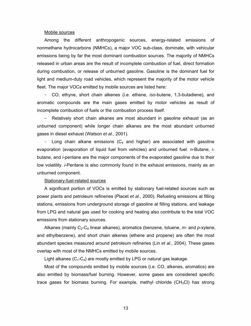
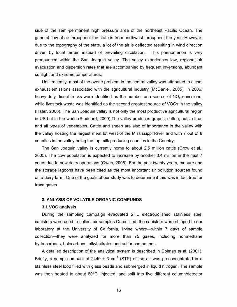
In an effort to highlight differences in the VOC sources for the different source

regions in the investigated area, we segregated the samples collected during the four

CARB flights and the two transits (Flight 16 and Flight 24) in four main groups: samples

collected over the SCAB region and specifically over the LA area, over the SJV, over

San Diego, and over the border between Mexico and the U.S. Figures 11-a through 11-d

illustrate the position of the samples collected within these different regions.

Figure 11-a. Geographical location of the samples collected over the SJV.

Figure 11-b. Geographical location of the samples collected over the LA area.

-119.4 -119.0 -118.6 -118.2 -117.8

32.8

33.2

33.6

34.0

34.4

34.8

-123 -122 -121 -120 -119 -11831.5

32.0

32.5

33.0

33.5

34.0

31.5

32.0

Longitude

Longitude

Latitude

Latitude

30

Figure 11-c. Geographical position of the samples used to represent the SCAB

region.

Figure 11-d. Geographical position of the samples collected over the San Diego area

(red “plus”) and over the border between Mexico and the U.S (blue “plus”).

-118 -117.5 -117 -116.5 -116 -115.5 -11531.5

32.0

32.5

33.0

33.5

34.0

San Diego

-121 -120 -119 -118 -117 -116 -115

32

33

34

35

36

Longitude

Longitude

Latitude

Latitude

31

5.2 CFC replacement compounds

We present here the distribution of the halocarbon fraction measured over California

focusing on CFC replacement compounds in response to one of the main objective of

the ARCTAS-CARB mission (i.e. provide observations to improve emission inventories

for greenhouse gases).

HCFCs and HFCs have been introduced as substitute of CFC compounds in

response to the regulations imposed by the Montreal Protocol and subsequent


layer, the chlorine-free compound HFCs do not pose any treat to the ozone layer.

However, because of their ability to absorb infrared radiation, HFCs are important

greenhouse gases enhancing radiative forcing.

Figures 12-15 show the mixing ratios measured for the samples collected during the

four ARCTAS-CARB flights and the two transits (flights 16 and 24) over the source

regions previously presented.

HCFC-22

0

100

200

300

400

500

600

700

800

900

1000

-10 90 190 290 390 490Samples

Mix

ing

Ra

tio, p

ptv

LA SCAB San Diego SJ Valley Mexico Border

Figure 12. HCFC-22 mixing ratios.

288 ± 109 pptv over LA basin 191 ± 2.8 pptv background

32

HCFC-142b

0

100

200

300

400

500

600

700

800

900

-10 90 190 290 390 490Samples

Mix

ing

Ra

tio, p

ptv


Figure 13. HCFC-142b mixing ratios

HCFC-141b

0

50

100

150

200

250

-10 90 190 290 390 490Samples

Mix

ing

Ra

tio, p

ptv


Figure 14. HCFC-141b mixing ratios

58 ± 118 pptv over LA basin 19.0 ± 0.4 pptv background


33

HFC-134a

0

100

200

300

400

500

600

700

800

-10 90 190 290 390 490Samples

Mix

ing

Ra

tio, p

ptv


Figure 15. HFC-134a mixing ratios.

HFC-152a

0

50

100

150

200

250

300

350

400

-10 90 190 290 390 490Samples

Mix

ing

Ra

tio, p

ptv


Figure 16. HFC-152a mixing ratios.

94 ± 76 pptv over LA basin 44 ± 0.8 pptv background


34

The trends illustrated in Figures 12-16 strongly suggest the presence of a significant

emission source of these gases over the LA area. Specifically, high enhancements in the

atmospheric levels of all the CFC replacements were measured over this source region.

The average levels (± 1-sigma SD) calculated over LA are summarized under each

plot and compared to the regional background calculated as the average of the lowest

quartile of the remaining ARCTAS-CARB samples collected below 8 km of altitude (to

avoid clean air from stratospheric intrusions).

5.3 HFC-152a emission estimates.

The highest increase with respect to the background was observed for HCF-152a

with an average mixing ratio about 10 times higher.

HFC-152a levels have been exponentially increasing in the atmosphere in the past

decade (particularly in the northern hemisphere; Table 3) with the highest emissions

sources located in North America.

Table 3. HFC-152a emissions from different locations – literature data

Year Location Emissions (Gg/yr)

1995-98 Europe 0.46 (a)

2000-01 Europe 0.8 (a)

2003 Europe 2 (a)

2003-04 Europe 1.5 - 4.0 (a)

2006 North America 16 (b)

2006 U.S. 12 (b)

2004 Australia 0.005 – 0.01 (a)

Late 1990s Global 4 (a)

2002-03 Global 20 - 22 (a)

2004 Global 28 (a)

2006 Global 37 (b)

(a) Greally et al., 2007. (b) Stohl et al., 2009.

Figure 17 shows the geographical location of the samples collected over the LA

basin color coded by HFC-152a levels. Particularly high mixing ratios were observed

35

south-east of downtown. Some of the samples collected offshore were also

characterized by elevated HFC-152a levels.

Figure 17. Mixing ratio of HFC-152a measured over the LA area during the

ARCTAS-CARB flights.

In an effort to extrapolate the HFC-152a emissions from the LA basin we multiplied

the HFC-152a/CO mass ratio (Figure 18) by the CO annual emission from the LA county

reported by CARB (1958 tons per day – 2 x 109 grams per day [3]).

150 134 118 102 86 70 54 38 22 6

Mixing ratio, pptv

36

y = 0.59x - 56

R2 = 0.82

0

20

40

60

80

100

120

140

50 100 150 200 250 300 350

CO, ppbv

HF

C-1

52a,

ppt

v

Molar ratio (mmol / mol)0.59 ± 0.03

Figure 18. Plot of HFC-152a versus CO for the samples observed over the LA area.

To obtain the mass ratio, the HFC-152a/CO volume ratio (pptv/ppbv or mmol/mol)

was multiplied by the respective molecular weights:

0.59•10-3 (molHFC152a/molCO) × 66 (g/mol)HFC-152a / 28 (g/mol)CO × 2•109

(g/day)CO × 365 days/yr = 1.0 Gg/yr

According to the above calculation, we extrapolate a HFC-152a emission of 1.0

Gg/yr from the LA county. One way to estimate total emissions of HFC-152a is to use

population data for LA and the US.

= 31 Gg/yr (U.S.) = U.S. estimate for 2008

According to Greally et al. (2007) [1], HFC-152a global emissions for the 1994-2004

period increased at a rate of about 14% per year. This increase gives a global estimate

of about 45 Gg/yr for 2008. The 31 Gg/yr extrapolated for the U.S. using the ARCTAS-

CARB data represents ~ 68% of the global emissions.

1.0 Gg/yr (LA county)

9.9•106 (population in LA county) 304•106 (U.S. population) = ×

37

Air quality simulations were performed using the UCI-CIT Air Quality Model, which is

a three-dimensional Eulerian urban photochemical model designed to study the

dynamics of pollutant transformation and transport in the SCAB. The UCI-CIT model

uses a horizontal 80x30 rectangular grid with 5 vertical layers. Each grid cell

corresponds to a 5km x 5km region extending 1100m in height. The model includes the

CalTech Atmospheric Chemistry Mechanism (Griffin et al., 2002a; 2002b) which consists

of 445 gas-phase chemical reactions and 137 gas-phase species. The temperature,

wind fields, and other meteorological parameters are taken from the September 8-9,

1993 field campaign described in Griffin et al. (2002b). In the simulations, HFC-152a is

emitted from urban areas at a constant rate of 1.2×10-5 g m-2 hr-1 between 6 am and 10

pm. Although HFC-152a may react with OH at a rate of 3.5×10-14 cm3 molec-1 s-1 (at 298

K), loss due to chemical reaction is insignificant compared to loss from transport. The

UCI-CIT model is run for five simulation days allowing the system to reach a steady

diurnal cycle of HFC-152a. The data presented here is from the final simulation day.

Figure 19 shows a contour plot of the concentration of HFC-152a in the entire SCAB at

noon.

Figure 19. HFC-152a levels in the SCAB at noon.

12:00 pm

38

The mixing ratios measured during the ARCTAS-CARB flights over the LA area (i.e.

about 50 pptv average) are correctly predicted by the model and the emissions of

1.2×10-5 g m-2 hr-1 used in the simulation agree very well with the emission extrapolated

from the HFC-152a/CO slope (~ 1.1 Gg/yr vs 1.0 Gg/yr).

6. Oxygenated compounds

6.1 Airborne data used in Dairy Emissions Analysis

The data used in this section were obtained during a total of seven flights including

two test flights and five science flights. Test flights were conducted in order to provide all

researchers aboard the NASA DC-8 aircraft an opportunity to not only calibrate their

instruments but to also ensure that the instruments were operating at optimum capacity.

Out of the remaining five science flights, four of them were flights which were a part of

the ARCTAS-CARB study, while the final research flight consisted of a low-level

segment through the San Joaquin valley as part of the transit back into California from

Cold Lake, Canada (i.e. Flight 24).

The four flights that engaged in low-level runs through the valley were test flights (TF)

1 and 2, science flight (SF) 13 and transit flight (TF) 24. A summary of the flights and

their durations is presented in table 4.

Table 4: Summary of flights that were analyzed for emissions from dairy farms.

Flight Date Duration Hours of flight (PST) Ave. Temp in SJV (C)

TF 1 3/18/08 3 hrs 35 mins 11.05 am to 2.40 pm 20


SF 13 6/20/08 7 hrs 48 mins 10.32 am to 6.15 pm 38


With the exception of selected atmospheric source tracers, fewer compounds were

analyzed on the test flights compared to the science flights as most of the instruments

on the plane were not involved in data collection but in the process of instrumental

calibration. The data presented for both test flights primarily consists of data (whole air)

collected by the UCI team.

39

6.2 Effects of California Wild fires on airborne data

Every year California faces the threat of fire season. The emissions from biomass

burning not only affect the air quality on the ground, but also extend up into the free

troposphere. Evidence of biomass burning is seen in the data through the quantification

of specific biomass burning tracers. These include CO, CH4 and CH3Cl. During all four

ARCTAS-CARB flights, evidence of wild fires burning in California can be observed. By

the month of June, the wild fires had been burning for approximately three months

causing the SJV to be inundated with smoke. For flights 13 and 24, we are unable to

distinguish between the biomass burning emission sources of the air masses observed

at 1000 ft in altitude and other individual emission sources in the SJV. The extent to

which the biomass burning emissions have consumed the SJV air basin is shown in

figure 20.

Figure 20. MODIS image of California taken on June 20th, 2008, with major cities and

significant wild fires highlighted in the image (UMBC, 2008).

Photochemical reactions of the compounds emitted from biomass burning must also

be considered as many short-lived gaseous species react in the atmosphere to form

secondary products. For example, one of the compounds given off by biomass burning

is formaldehyde (CH2O). In the atmosphere, CH2O is able to photodissociate to produce

40

carbon monoxide (CO) and the very reactive perhydroxyl (HO2) radical, as shown in the

reaction below (Holzinger et al., 1999):

CH2O + h (+2O2) → CO + 2HO2 (9)

This HO2 radical can then react with several other species in the atmosphere. The

CO produced in this reaction may also interfere with our measurement of CO, as an

urban tracer.

An important biomass burning tracer used in this study is methyl chloride (CH3Cl;

with an average background level in the atmosphere of about 550 pptv). All the flights

showed elevated levels of CH3Cl 1000 ft above the valley floor.

Since the fire season didn’t begin till March 2008, and both test flights 1 and 2

occurred at the beginning of the flare up, the effect of biomass burning on the overall

data is still minimal and distinguishable from other emission sources. By examining the

two main biomass burning tracers, CH4 and CH3Cl, we are able to distinguish between

biomass burning plumes and all other sources (dairy and urban/industrial sources). By

plotting biomass burning tracers against each other, and measuring their correlations,

we are able to isolate biomass burning plumes within the air mass sampled. Figure 21

shows CH4 versus CH3Cl, with the different plumes highlighted in different colors.

41

Figure 21. Test flight 2: Analysis of the data collected over the entire flight in search

for emissions originating from biomass burning sources.

Within the biomass burning plume, as highlighted by the yellow points in figure 21,

both CH4 and CH3Cl are well correlated with a coefficient of determination (R2) value of

0.73. However, within the hypothesized dairy plume, as indicated by the pink points in

figure 21, there is no correlation (R2 value of 0.04). Similarly, the remaining air masses

analyzed for test flight 2 (blue points in figure 21) show a poor correlation between CH4

and CH3Cl with a R2 value of 0.1. Based on the correlations alone, we can conclude that

a portion of air mass sampled in test flight 2 had a biomass burning source, and that not

all of the methane present in the SJV is a product of dairy farming. Figure 21 illustrates

the importance of using tracers in order to analyze emission sources in the atmosphere.

6.3 Significance of “urban” tracers

To differentiate between different emission sources it is important to isolate urban

emissions from dairy farm emissions. This is especially important for key compounds

such as methanol and acetone which may have more than one contributing source in the

SJV. The two VOCs commonly used to distinguish urban air masses are CO and ethyne

42

(C2H2), which are the main exhaust components of internal combustion engines (Barletta

et al., 2002). The photochemical lifetime of CO and C2H2 is about two months and three

weeks respectively (Khalil et al., 1990; Simpson et al., 2004). In the airborne data set,

CO was measured in situ on the NASA DC-8 airplane by the differential absorption CO

measurement (DACOM) instrument (Sachse et al., 1987).

There are two industrial solvents that are also used as urban/industrial tracers -

perchloroethylene (C2Cl4) and tetrafluoroethane (HFC-134a). The photochemical lifetime

of C2Cl4 and HFC-134a are 3-4 months and 14 years respectively (Simpson et al., 2004;

McCulloch et al., 2003). The current atmospheric mixing ratios of C2Cl4 and HFC-134a

are 5-10 pptv and ~ 50 pptv respectively (Simpson et al., 2004; O’Doherty et al., 2008).

All of these urban tracers have long strong anthropogenic sources and reasonably long

lifetimes allowing them to be observed in remote air.

Based on the data obtained in previous flux chamber studies and the estimates of

ventilation within the valley, it appears that there are other significant emission sources

of ethanol within the SJV besides the silage piles on dairy farms. Based on its lifetime,

we do not expect ethanol to have reacted by the time they have reached an altitude of

1,000 ft above the valley floor. In the airborne data, we are able to clearly distinguish

between urban/industrial sources and dairy farm sources. In test flight 1, the presence of

an urban/industrial source of ethanol is examined by plotting CO against ethanol (figure

22). Based on the graph, two distinct trends are observed, each corresponding to a

specific emission source. We make the assumption that the trend with the pink points in

the plot corresponds to emissions from dairy farms, while the other remaining blue points

in the plot corresponds to emissions from an urban/industrial source. The correlation of

CO and ethanol within the dairy plume is weak with a R2 value of 0.31 while the same

correlation within the remaining air mass is stronger with a R2 value of 0.67. Based on

the correlations, it is clear that there are two different sources of ethanol within the SJV,

one with a greater urban/industrial source origin than the other. Hence, we can use the

R2 value correlations in this case in order to identify individual source emissions.

43


for emissions originating from urban/industrial sources and dairy farm sources.

Similarly, when we plot another urban/industrial tracer, C2Cl4 against ethanol, we

have a similar graph as shown in figure 23.

44


for emissions originating from urban/industrial sources using the tracer, C2Cl4.

Once again, two trends are evident in the data corresponding to two different

emission sources. In figure 23, the correlation between C2Cl4 and ethanol in the dairy

plume is lower (R2 = 0.10) than that of all other samples taken during the flight over

California (R2 = 0.77). Similar plots are observed for test flight 2, science flight 13 and

transit flight 24. We are able to identify the dairy plume based on its weak correlations

with specific urban/industrial tracers as well as the enhanced levels of ethanol observed

with relative constant level of urban/industrial tracers within the plume. This would not be

the same in the case of an urban/industrial plume, in which both compounds would be

elevated. We can further illustrate this point by plotting the two urban/industrial tracers

against one another. Figure 24 is a plot of CO against C2Cl4 mixing ratios observed in

test flight 1.

45

Figure 24. Test flight 1: Analysis of the data collected over the entire flight. The plot

of CO against C2Cl4 is color-coded showing the separation of sources within the air

mass sampled in the flight above California.

Figure 24 is color-coded showing the separation of the air mass measured during the

flight into different sources. As observed in figure 22, in the dairy plume, the CO mixing

ratio did not exceed 174 ppbv, while the C2Cl4 mixing ratio did not exceed 7.3 pptv. The

lower values of CO (< 150 ppbv) and C2Cl4 (< 4.5 pptv) observed in figure 24 are high

altitude samples and are representative of “clean” background air.

6.4 Effects of dairy farming on air quality in the SJV

The data obtained from the airborne study allowed us to conduct a “top down”

assessment of the impact selected oxygenates have on SJV air quality. Table 5 lists the

average oxygenate levels found in the SJV legs of the 4 flights through California. The

average of the samples collected above 20,000 ft is here considered representative of

the background.

46

Table 5. Summary of the average mixing ratios observed for four oxygenates and

methane during the four flights over the SJV. Units: ppbv.

Sampling location Ethanol Methanol Acetaldehyde Methane

Background average (> 20,000 ft) 0.55 0.54 0.24 1800

Test flight 1 average (1,000 ft) 2.0 4.7 0.9 2040

Test flight 2 average (1,000 ft) 2.4 3.9 0.7 2010

Flight 13 average (1,000 ft) 2.3 5.8 0.9 1980

Flight 24 average (1,500 ft) 2.4 6.3 1.3 1930

In order to determine if any trends are present in the emissions of each oxygenate,

emission ratios are used. Based on the ethanol and methanol mixing ratios presented in

Table 5, we can determine the average ethanol to methanol (C2H5OH/CH3OH) ratio for

each flight. The C2H5OH/CH3OH ratios for test flights 1 and 2, science flights 13 and 14

are 0.43, 0.62, 0.39 and 0.38 respectively versus a C2H5OH/CH3OH average ratio of

1.03 in the background. This suggests that by the time ethanol and methanol reach the

troposphere, the ratio of one to the other is approximately 1. The lower ratios observed

during the flights (especially flights 13 and 14) suggest the presence of elevated

methanol levels compared to ethanol levels. There are several possible explanations for

this which will be discussed in the next section.

6.5 Alternate sources of methanol in the SJV

Looking at the airborne data, methanol levels at the surface are elevated significantly

above background, suggesting the presence of an additional methanol source in the SJV.

Other sources of methanol besides biomass burning may also be present in the valley,

however, at this point in our research, we are unable to determine if and what they might

be. Similarly, the same argument for elevated methanol levels can be applied to flights

13 and 24. As mentioned earlier, by this point in the fire season, the emissions from the

wild fires had permeated throughout the valley, resulting in a well mixed layer trapped in

the SJV. As the emission source of methanol had been fairly strong and consistent for

months, by the months of June and July, the average methanol level observed

throughout the valley was uniformly elevated as compared to background levels.

Exceptions to this were active large wild fires, which created hot spots of elevated

biomass burning emissions above the already elevated levels which were impacting the

valley air basin. The emissions from the fires mask the relatively lower level emissions of

47

methanol from dairy farms, hence making it difficult for us to use methanol as a tracer for

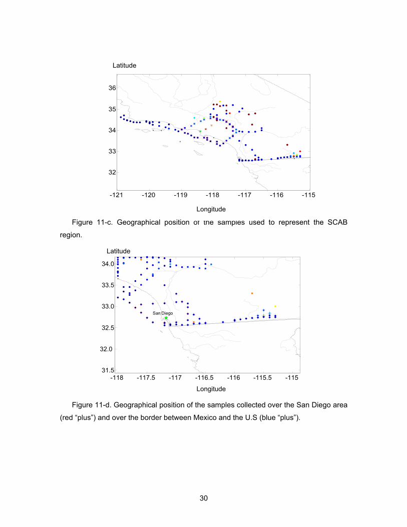
dairy farms in the SJV for flights 13 and 24. Figure 25 is a graph plotting methanol

mixing ratios for flight 13. The hot spots of methanol observed correspond with major

wild fires burning in California in the week of June 20th, 2008, as shown in figure 26.

Google earth plots are used in both figures 25 and 26 in order to provide a clear

comparison between the MODIS fire imagery of California and the observed methanol

mixing ratios.

Figure 25. Google earth plot of methanol mixing ratios observed for science flight 13

through California on June 20th, 2008.

48

Figure 26. MODIS imagery of the California wild fires burning in the week of June

20th, 2008 (UMBC, 2008).

Due to the emissions from the wild fires, and its effects on the ethanol to

methanol ratio, we are unable to use the measured methanol mixing ratios for both

flights 13 and 24. All the flights showed elevated levels of acetone compared to

background levels measured at 20,000 ft. Both flights 13 and 24 also show elevated

levels of acetaldehyde compared to those measured in test flights 1 and 2. Just like

methanol, Holzinger et al. (1999) report the emissions of both acetone and acetaldehyde

from biomass burning. The estimated global emissions of acetone and acetaldehyde

from biomass burning are determined to be (2.3 1.2 to 6.1 3.1) Tg and (3.8 1.6 to

10 4.2) Tg respectively (Holzinger et al., 1999). Again, due to the effects biomass

burning emissions have on the average mixing ratios of the 4 oxygenates found in the

valley, we are unable to use flights 13 and 24 to accurately determine the effects that

dairy oxygenate emissions have on the SJV air basin. It is interesting to note though, for

reasons unknown, despite methane being a well-known biomass burning tracer, the

49

average methane mixing ratio observed for flight 24 is lower than all of the 3 other valley

flights.

6.6 Average ethanol mixing ratios observed in the SJV

The average ethanol mixing ratio observed is overall constant throughout the valley

for all 4 flights. Figure 27 and 28 are plots of the ethanol mixing ratios observed in both

test flights 1 and 2. The ethanol hot spots of elevated ethanol mixing ratios correspond

to the nation’s top three dairy producing counties, hence the counties with the most

number of dairy cows.

Figure 27: Test flight 1: Ethanol mixing ratios observed throughout the entire flight

over the state of California.

Mixing ratio (pptv)

50

Figure 28. Test flight 2: Ethanol mixing ratios observed throughout the entire flight


Both test flights show elevated levels of ethanol (>1500 pptv) mainly throughout the

low level leg of the flight through the SJV. If we make the assumption that all the ethanol

being emitted in the valley is from dairy farms alone, and that the average ethanol mixing

ratio in the valley is 2.2 ppbv at 1000 ft, with dairy farms as the source, the

C2H5OH/CH3OH ratio observed for test flight 1 is about 0.5. Figures 29 and 30 show

similar plots for methanol mixing ratios observed in both test flights 1 and 2.

Mixing ratio (pptv)

51

Figure 29. Test flight 1: Methanol mixing ratios observed throughout the entire flight


Figure 30. Test flight 2: Methanol mixing ratios observed throughout the entire flight


Mixing ratio (pptv)

Mixing ratio (pptv)

52

As mentioned earlier, methane can also be used as a tracer for dairy farm emissions.

Despite the average methane mixing ratios reported in table 5 being only slightly higher

than background, we are still able to detect elevated levels of methane through the SJV,

corresponding to intense dairy farm activity. Figures 31 and 32 are plots of methane

mixing ratios observed during both test flights 1 and 2.

Figure 31. Test flight 1: Methane mixing ratios observed throughout the entire flight


Mixing ratio (ppbv)

53

Figure 32. Test flight 2: Methane mixing ratios observed throughout the entire flight


Mixing ratio (ppbv)

54

7. Final report Technical Sub-Contract

To the University of California, Irvine For submission to the California Air Resources Board

ARCTAS- California 2008: An airborne mission to investigate California air quality

Principal Investigator

Ronald C. Cohen

Professor, Department of Chemistry and Department of Earth and Planetary Science

University of California, Berkeley Berkeley, CA 94720-1460

(510) 642-2735 (510)643-2156 (FAX)

e-mail: [email protected]

This subcontract provided support to a joint UCI, UC Berkeley, NASA proposal aimed at making observations of atmospheric composition in California in support of ARB regulatory objectives with respect to air quality and climate change. Tasks the Cohen team at Berkeley contributed to the ARCTAS-California 2008 experiments were as follows.

1) Integrate instrument for measurement of NO2, total peroxynitrates, total alkyl and multifunctional nitrates and HNO3 aboard the NASA DC-8.

2) Participate in flight planning discussions using recent experience in BEARPEX and other California ground based experiments and modeling analyses as a guide.

3) Complete final data from the Berkeley measurements and report to the NASA archive. Provide aid to ARB, if desired, in making the complete NASA archive of all measurements in CA as a separate data file.

4) Initial observation based analyses: Although final analyses will require more time than is provided under this contract, the Berkeley group plans to focus its efforts on observation based analyses aimed at using observations to assess correlated sources of VOC and NOx, sources of NOx alone and the effects of NOx on a) HOx radicals, b) inorganic and organic aerosol production and c) production of O3. We expect to provide initial assessment of progress in these areas during this contract and then to complete analyses and publish them with continued NASA support after the expiration of this contract.

Tasks 1 and 3: Observations

The bulk of the effort for this subcontract was dedicated to tasks 1 and 3. The instrument was integrated into the payload as required by the schedule and final data from the mission was reported to the archive by the required deadlines. Observations were reported for all of the flights as the instrument performed flawlessly. The measurements

55

we made were of NO2, total peroxynitrates (ΣPNs), and total alkyl and multifunctional nitrates (ΣANs). As there were two other HNO3 instruments aboard the plane we did not emphasize HNO3 measurements, instead devoting more attention to the other three chemical species. The measurements were made using the method of thermal-dissociation laser-induced fluorescence (Day et al. 2002, Thornton et al. 2000).

Briefly, observations described here were made aboard the NASA DC-8. NO2, ΣPNs, and ΣANs were measured using the Berkeley thermal dissociation-laser induced fluorescence instrument (Day et al., 2002; Thornton et al., 2000). Briefly, gas is pulled simultaneously through three channels consisting of heated quartz tubes maintained at specific temperatures for the dissociation of each class of compounds above. Each heated section is followed by a length of PFA tubing leading to a detection cell where NO2 is measured using laser-induced fluorescence. Due to differing X-NO2 bond strengths, ΣPNs, ΣANs and HNO3 all thermally dissociate to NO2 and a companion radical at a characteristic temperature. The ambient channel measures NO2 alone, the second channel (180˚C) measures NO2 produced from the dissociation of ΣPNs in addition to ambient NO2 (the observed signal is NO2+ΣPNs) and the third channel (380˚C) measures NO2+ΣPNs+ΣANs. Concentrations of each class of compound correspond to the difference in NO2 signal between two channels set at adjacent temperatures. The difference in NO2 signal between the 180˚C and the 380˚C channel, for example, is the ΣANs mixing ratio. The instrument deployed for ARCTAS had a heated inlet tip that split in two immediately. One third of the flow was immediately introduced to heated quartz tubes for detection of ΣANs while the other two-thirds was introduced to an additional heated quartz tube for detection of ∑PNs and an ambient temperature channel for detection of NO2.

Ambient NO2 and NO2 produced by thermal dissociation were observed by laser-induced fluorescence as described in detail by Thornton et al. (2000). Briefly, a tunable dye laser is pumped at 7 kHz by a Q-switched, frequency doubled Nd+3YAG laser. The incoming gas is cooled through the use of a supersonic expansion (Cleary et al., 2002) and the dye laser, utilizing Pyrromethene 597 in isopropanol, is tuned to an isolated rovibronic feature of jet-cooled NO2 at 585 nm. The frequency is held for 9 seconds at the peak of this feature and then for 3 seconds at an offline position in the continuum absorption. The ratio of peak to background fluorescence of the chosen feature is 10 to 1 at 1atm and the difference between the two signals is directly proportional to the NO2 mixing ratio. The laser light is focused in series through two multi-pass (White) cells (discussed in more detail below) and the red-shifted fluorescence is detected using a red-sensitive photomultiplier tube (Hamamatsu). Fluorescence counts are collected at 4 Hz, scattered light at wavelengths less than 700nm is rejected by band-pass filters and time-gated detection is used to eliminate noise resulting from scattered laser light in the cell. We observe a dependence of NO2 fluorescence on the external pressure. We calibrate the NO2 LIF vs. altitude by direct measurement of NO2 from a standard addition during a test-flight. Calibrations were performed at least once every two hours during a level flight leg using a 4.5ppm NO2 reference gas with a stated certainty of +/- 5%. The reference gas was compared to a library of standards in lab both before and after the campaign. The individual standards are compared on a regular basis (about every 6 months) to ensure stability and highlight when a given tank has degraded. These standards have been observed to remain stable for up to 5 years and to be accurate at atmospherically relevant mixing ratios to within 1% (Bertram et al., 2005).

The instrument deployed for ARCTAS had two detection cells. The direction of flow into the cell was controlled using a three-way valve and a bypass pump was used to

56

maintain flow in the non-sampled channel. Cell 1 sampled the ambient channel continuously while cell 2 sampled either the 180oC (50% of the time) or the 380oC channel (50% of the time). Thus for every 2 minute duty cycle there were ten 9s average measurements of NO2, five 9s average measurements of ΣPNs, and five 9s average measurements of sum (∑PNs+∑ANs). As the ∑ANs measurement is a subtraction, the uncertainty depends both on ∑ANs and on the sum (NO2+∑PNs). For example, if there were 100ppt each of NO2 and ∑PNs, the precision of the ∑ANs measurement would be ~15 ppt in 20s. If there were 1 ppb each of NO2 and ∑PNs the precision of the ∑ANs would be 40 ppt.

The TD-LIF measurement of HNO3 has been shown to be the sum of aerosol and gas-phase HNO3 (Fountoukis et al., 2009) and we expect aerosol phase organic nitrates to behave similarly. Comparison of TD-LIF observations of an isoprene nitrate standard to observations made using a PTR-MS show both instruments to be consistent to within 10% (Perring et al., 2009). Comparisons of NO2 and ∑PNs have also been described and indicate similar or better accuracy for these species. (Thornton et al., 2003, Wooldridge et. al., 2009)

Observations of NO2, �PNs and �ANs during the four ARCTAS-CARB flights and the transit flight from California to Cold Lake, Canada are shown in the Figures 1-3.

Figure 1 NO2 measurements taken aboard the NASA DC-8 during the CARB-ARCTAS 2008 flights on June 18th, 20th, 22nd,and 24th, and on the June 26th transit flight to Cold Lake, Canada. Scale is log(NO2 ppt).

57

Figure 2 ΣPNs measurements taken aboard the NASA DC-8 during the CARB-ARCTAS 2008 flights on June 18th, 20th, 22nd,and 24th, and on the June 26th transit flight to Cold Lake, Canada. Scale is log(ΣPNs ppt).

Figure 3 ΣANs measurements taken aboard the NASA DC-8 during the CARB-ARCTAS 2008 flights on June 18th, 20th, 22nd,and 24th, and on the June 26th transit flight to Cold Lake, Canada. Scale is log(ΣANs ppt).

58

Task 2: Flight Planning

Flight planning was an active collaboration of DC-8 investigators, pilots and navigators and led by the CARB team. Cohen was an active participant in the discussions especially in helping to translate CARB objectives to the DC-8 community and to help to assess the capabilities of the aircraft to fly routes that were almost exclusively in the boundary layer.

Task 4: Analyses

Initial observation based analyses have been developed and results described at the ARCTAS Science team meeting and at the CARB-ARCTAS science team meeting. These analyses focus in on the role of RONO2 formation as a chain termination of ozone production and on the utility of the observations as a tool to evaluate satellite NO2 measurements.

RONO2 chemistry

We observed very high ratios of RONO2 to O3 in the LA Basin. Figure 4 shows the correlation between odd oxygen (O3+NO2) and ΣANs for urban locations (defined at NO ≥ 10% of NOy) in the LA Basin. Following the analysis of Rosen et. al. 2004, the inverse of the slope of this line should equal half the effective branching ratio for alkyl nitrate formation. This implies an effective branching ratio of 6% for the LA basin.

Figure 4 Correlation between Ox (= O3 + NO2) and total alkyl and multifunctional nitrates (ΣANs) for boundary layer measurements in urban areas of CA. Urban areas are defined as NO ≥ 10% of NOy. The slope of this line implies a branching ration of 6% for the formation of ΣANs from urban VOC mixtures.

Satellite validation

59

Figures 5 and 6 show a preliminary evaluation of the comparison of boundary layer NO2 as measured by the DC-8 with near coincident (in space and time) column NO2 measured from the OMI instrument aboard the Aura Satellite.

Figure 5 (Left) In-situ NO2 (ppb) from the NASA DC-8 during the ARCTAS CARB flights. (Right) OMI tropospheric NO2 (molecules/cm2) for June 2008.

Figure 6 Correlation between the tropospheric column derived from the in-situ measurements of NO2 aboard the NASA DC-8 and the OMI tropospheric column NO2.

Although there remain many details to investigate, the basic pattern supports the accuracy of the OMI retrieval. As shown in figure 6, the slope of the regression in this

60

preliminary analysis (R2=.72) is 0.82, possibly indicating the OMI retrievals are biased low by 18% during this season.

References

Bertram, T. H., Cohen, R. C., Thorn, W. J., and Chu, P. M., Measurement Consistency between O3, NO and NO2 Standards at Tropospherically Relevant Levels, J. Air and Waste Management Assoc., 55, 1473-1479, 2005. Cleary, P. A., Wooldridge, P. J., and Cohen, R. C., Laser-induced Fluorescence Detection of Atmospheric NO2 Using a Commercial Diode Laser and a Supersonic Expansion, Applied Optics, 41(33) 6950-6956, 2002. Day, D. A., Wooldridge, P. J., Dillon, M., Thornton, J, A, and Cohen, R. C., A Thermal dissociation-laser induced fluorescence instrument for in-situ detection of NO2, peroxy(acyl)nitrates, alkyl nitrates, and HNO3, J. Geophys. Res., 107(D6), 10.1029/2001JD000779, 2002. Fountoukis, C., Nenes, A., Sullivan, A., Weber, R., Van Reken, T., Fischer, M., Matias, E., Moya, M., Farmer, D., and Cohen, R. C., Thermodynamic characterization of Mexico City aerosol during MILAGRO 2006, Atmos. Chem. and Phys., 9, 2141-2156, 2009. Perring, A. E., Bertram, T. H., Wooldridge, P. J., Fried, A., Heikes, B. G., Dibb, J., Crounse, J. D., Wennberg, P. O., Blake, N. J., Brune, W. H., Blake, D. R., and Cohen, R. C., Airborne observations of total RONO2: new constraints on the yield and lifetime of isoprene nitrates, Atmos. Chem. Phys., 9, 1451-1463, 2009. Rosen, R. S., Wood, E. C., Wooldridge, P. J., Thornton, J. A., Day, D. A., Kuster, W., Williams, E. J., Jobson, B. T., and Cohen, R. C., Observations of total alkyl nitrates during Texas Air Quality Study 2000: Implications for O3 and alkyl nitrate photochemistry, J. Geophys. Res., 109, D07303, doi:10.1029/2003JD004227, 2004. Thornton, J. A., Wooldridge, P. J., and Cohen, R. C., Atmospheric NO2: In Situ Laser-Induced Fluorescence Detection at parts per trillion mixing rations, Anal. Chem., 72, 528, 2000. Thornton, J. A., Wooldridge, P. J., Cohen, R. C., Williams, E. J., Hereid, D., Fehsenfeld, F. C., Stutz J., and Alicke, B., Comparison of in situ and long path measurements of NO2 in urban plumes, J. Geophys. Res., 108(D16), 4496, doi:10.1029/2003JD003559, 2003.

61

Wooldridge, P. J., Perring, A. E., Bertram, T. H., Flocke, F. M., Roberts, J. M., Singh, H. B., Huey, L. G., Thornton, J. A., Murphy, J. G., Fry, J. L., Rollins, A. W., LaFranchi, B. W., and Cohen R. C., Total peroxy nitrates (ΣPNs) in the atmosphere: the thermal dissociation-laser induced fluorescence (TD-LIF) technique and comparisons to speciated PAN measurements,

Atmos. Meas. Rech. Discuss., 2, 3055-3097, 2009.

62

8. Conclusions

The analysis of the volatile organic compounds measured during the ARCTAS-

CARB phase highlights the presence of important emission sources within the SCAB

area for many gases. We were able to identify and quantify more than 60 gases and

characterize the VOC composition of different source regions within the SCAB.

Because of the increasing levels of CFC replacements in the atmosphere in the last

few years, and the increasing concern on the magnitude of their contribution to global

warming, we investigated the distribution of these species in greater detail. Among the

HFCs, we focused our attention on HFC-152a, one of the fastest increasing CFC

replacement compounds measured. Through the analysis of the HFC-152a versus CO

plot we first extrapolated a HFC-152a emission of 1.0 Gg/yr from the LA County, and

then used the population data to extrapolate HFC-152a emissions from the United

States. This study contributes to the present knowledge of the United States’ impact to

the global emissions of an important greenhouse gas.

Moreover, aircraft measurements aboard the DC-8 allowed us to determine both the

background level of some oxygenate in the valley as well as the enhancement level of

these oxygenates when flying at low altitude through the valley. Among these

compounds, we have found that ethanol, methanol, and acetaldehyde are produced in

major quantities throughout the San Joaquin valley as by-products of yeast fermentation

of silage and photochemical oxidation.

The data gathered during the CARB research flights were archived into the NASA website together with data obtained during the two ARCTAS deployments carried out before and after the CARB flights.

High quality nitrogen oxide measurements were submitted to a public archive. Investigations into our understanding of atmospheric chemistry using those measurements in concert with the measurements of dozens of NASA sponsored investigators are in progress.

63

9. References

Atlas, E., Pollock, W., Greenberg, J., Heidt, L., Thompson, A.M., 1993. Alkyl nitrates,

nonmethane hydrocarbons, and halocarbon gases over the equatorial Pacific Ocean during Saga

3. Journal of Geophysical Research, [Atmospheres], 98(D9), 16933-16947.

Barletta, B., Meinardi, S. Simpson, I., Khwaja, H., Blake, D.R., Rowland, F.S., 2002. Mixing

Ratios of Volatile Organic Compounds (VOCs) in the Atmosphere of Karachi, Pakistan.

Atmospheric Environment, 36 3429-3443.

Berntsen, T.K., Isaksen, I.S.A., Myhre, G.. Fuglestvedt, J.S., Stordal, F., Larsen, T.A.,

Freckleton, R.S., Shine, K.P., 1997. Effects of anthropogenic emissions on tropospheric ozone

and its radiative forcing. Journal of Geophysical Research, [Atmospheres], 102(D23), 28101-

28126.

Blake, N.J., Blake, D.R., Sive, B.C., Chen, T.-Y., Rowland, F.S. Collins, J.E., Jr., Sachse,

G.W., Anderson, B.E., 1996. Biomass burning emissions and vertical distribution of atmospheric

methyl halides and other reduced carbon gases in the South Atlantic region. Journal of

Geophysical Research, [Atmospheres], 101(D19), 24151-24164.

California Partnership for the San Joaquin Valley (CPSJV), 2007. Air Quality Action Plan.

Available on-line from http://www.sjvpartnership.org/action_plan.php?wg_id=2, accessed May

20th, 2009.

Colman, J.J., Swanson, A.L., Meinardi, S., Sive, B.C., Blake, D.R., Rowland, F.S., 2001.

Description of the analysis of a wide range of volatile organic compounds in whole air samples

collected during PEM- Tropics A and B. Analytical Chemistry 73, 3723-3731.

Crow, D., 2005. Air Pollution Control Officer’s Determination of VOC Emission Factors for

Dairies. San Joaquin Valley Air Pollution Control District.

Daum, P.H., Kleinman, L.I., Springston, S.R., Nunnermacker, L.J., Lee, Y.-N., Weinstein-

Lloyd, J., Zheng, J., Berkowitz, C.M., 2004. Origin and properties of plumes of high ozone

observed during the Texas 2000 Air Quality Study (TexAQS 2000). Journal of Geophysical

Research, [Atmospheres], 109(D17306), doi:10.1029/2003JD004311.

Greally, B.R., Manning, A.J., Reimann, S., McCulloch, A., Huang, J., Dunse, B.L., Simmonds,

P.G., Prinn, R.G., Fraser, P.J., Cunnold, D.M. O’Doherty, S., Porter, L.W., Stemmler, K., Vollmer,

64

M.K., Lunder, C.R., Shmidbauer, N., Hermansen, O., Arduini, J., Salameh, P.K., Krummel, P.B.,

Wang, R.H.J., Folini, D., Weiss, R.F., Maione, M., Nickless, G., Stordal, F., Derwent, R.G., 2007.

Observations of 1,1-difluoroethane (HFC-152a) at AGAGE and SOGE monitoring stations in

1994-2004 and derived global and regional emission estimates. Journal of Geophysical Research,

112, D06308, doi:10.1029/2006JD007527.

Griffin, R.J., Dabdub, D., Kleeman, M.J., Fraser, M.P., Cass, G. R., Seinfeld, J.H., 2002b.

Secondary organic aerosol. 3. urban/regional scale model of size- and composition-resolved

aerosols. Journal of Geophysical Research, 2002, 107, 4334.

Griffin, R.J., Dabdub, D., Seinfeld, J.H., 2002a. Secondary organic aerosol. 1. Atmospheric

chemical mechanism for production of molecular constituents. Journal of Geophysical Research,

107, 4332.

Hafer, J., 2006. San Joaquin Valley Air Pollution Control District Town Hall Meeting: Ozone

Plan. Discussion paper. Available on-line from

http://www.valleyair.org/Town_Hall/docs/Discussion%20Paper%20July%20Town%20Hall.pdf,

accessed June 19th, 2009.

Hellen, H., Kukkonen, J., Kauhaniemi, M., Laurila, T., Pietarila, H., 2005. Evaluation of

atmospheric benzene concentrations in the Helsinki Metropolitan Area in 2000-2003 using

diffusive sampling and atmospheric dispersion modeling. Atmospheric Environment, 39(22),

4003-4014.

Holzinger, R., C. Warneke, A. Hansel, A. Jordan, W. Lindinger, D.H. Scharffe, G. Schade, P.J.

Crutzen, 1999. Biomass burning as a source of formaldehyde, acetaldehyde, methanol, acetone,

acetonitrile, and hydrogen cyanide, Geophysical Research Letters, 26, 1161–1164.

Intergovernmental Panel on Climate Change (IPCC) 2001. Houghton, J.T., et al. (Eds),

Climate Change 2001 – The Scientific Basis. Cambridge, UK, 2001.

Kleinman, L.I., Daum, P.H., Imre, D., Lee, Y.-N., Nunnermacker, L.J., Springston, S.R.,

Weistein-Lloyd, J., Rudolph, J., 2002. Ozone production rate and hydrocarbon reactivity in 5

urban areas: a cause of high ozone concentration in Houston. Geophysical Research Letters,

29(10), 105/1-105/4.

Lin, T.Y., Sree, U., Tseng S.H., Chiu, K.H., Wu, C.H., Lo, J.G., 2004. Volatile organic

compound concentrations in ambient air of Kaohsiung petroleum refinery in Taiwan. Atmospheric

Environment, 38(25), 4111-4122.

65

Lindberg, J. 2007. Analysis of the San Joaquin Valley 2007 Ozone Plan. State of California

Air Resources Board. Final Draft Staff Report.

McCulloch, A., Ashford, P., and Midgley, P.M., 2001. Historic emissions of

fluorotrichloromethane (CFC-11) based on a market survey. Atmospheric Environment, 35(26),

4387-4397.

McCulloch, A., Aucott, M.L., Benkovitz, C.M., Graedel, T.E., Kleiman, G. Midgley, P.M., Li,

Y.-F., 1999. Global emissions of hydrogen chloride and chloromethane from coal combustion,

incineration and industrial activities: Reactive Chlorine Emissions Inventory. Journal of

Geophysical Research, [Atmospheres], 104(D7), 8391-8403.

McCulloch, A., Midgley, P.M., Ashford, P., 2003. Releases of refrigerant gases (CFC-23,

HCFC-22 and HFC-134a) to the atmosphere. Atmospheric Environment, 37(7), 889-902.

McDaniel, D., 2005. Clean Air – Collaborating to Reduce Diesel Emissions. Region 9: 2005

Progress Report. US EPA. Available on-line from

http://www.epa.gov/region09/annualreport/05/air.html, accessed June 18th, 2009.

O’Doherty. S., P.G. Simmonds, and G. Spain, 2008. Advanced Global Atmospheric Gases

Experiment – Annual Report. University of Bristol. Project No. GA01081. Available on-line from

http://209.85.173.132/search?q=cache:K68qfEAKGu4J:randd.defra.gov.uk/Document.aspx%3FD

ocument%3DGA0201_7766_ANN.doc+C2Cl4+lifetime+in+the+atmosphere&cd=21&hl=en&ct=cln

k&gl=us&client=safari, accessed May 13, 2009.

Owen, J., 2005. California Cows Fail Latest Emissions Test. National Geographic News.

Available on-line from

http://news.nationalgeographic.com/news/2005/08/0816_050816_cowpollution.html, accessed

June 18th, 2009.

Placet, M., Mann, C.O., Gilbert, R.O., Niefer, M.J., 2000. Emissions of ozone precursors from

stationary sources: a critical review. Atmospheric Environment, 34(12-14), 2183-2204.

Quack, B., and Wallace, D.W.R., 2003. Air-sea flux of bromoform: Controls, rates, and

implications. Global Biogeochemical Cycles, 17(1), 1023, doi:10.1029/2002GB001890.

Sachse, G., G. Hill, L. Wade, and M. Perry, 1987. Fast-Response, High-Precision Carbon

Monoxide Sensor Using a Tunable Diode Laser Absorption Technique, Journal of Geophysical

Research, 92(D2), 2071–2081.

66

Shine, K.P., 2001. Atmospheric ozone and climate change. Ozone: Science & Engineering,,

23(6), 429-435.

Simpson, I. J., S. Meinardi, N. J. Blake, F. S. Rowland, and D. R. Blake, 2004. Long-term

decrease in the global atmospheric burden of tetrachloroethene (C2Cl4). Geophysical Research

Letters, 31, L08108, doi:10.1029/2003GL019351.

Singh, H.B., Salas, L.J., Chatfield, R.B., Czech, E., Fried, A., Walega, J., Evans, M.J., Field,

B.D., Jacob, D.J., Blake, D., Heikes, B., Talbot, R., Sachse, G., Crawford, J.H., Avery, M.A.,

Sandholm, S., and Fuelberg, H., 2004. Analysis of the atmospheric distribution, sources, and

sinks of oxygenated volatile organic chemicals based on measurements over the Pacific during

TRACE-P. Journal of Geophysical Research, [Atmospheres], 109(D15S07),

doi:10.1029JD2003003883.

Smith, L., 2008. California Ambient Air Quality Standards (CAAQS). California Air Resources

Board. Available on-line from http://www.arb.ca.gov/research/aaqs/caaqs/caaqs.htm, accessed

May 25th, 2009.

Stoddard, E., 2009. FACTBOX: Water scarcity and agriculture in California. Thomson

Reuters 2009. Available on-line from

http://www.reuters.com/article/environmentNews/idUSTRE52C08M20090313, accessed June

17th, 2009.

Stohl, A., Seibert, P.,Arduini, J., Eckhardt, S., Fraser, P., Greally, B.R., Lunder, C., Maione,

M., Muhle, J., O’Doherty, S., Prinn, R.G., Reimann, S., Saito, T., Schmidbauer, N., Simmonds,

P.G., Vollmer, M.K., Weiss, R.F., Yokouchi, Y., 2009. Atmospheric Chemistry and Physics, 9,

1597-1620.

Sturrock, G.A., Etheridge, D.M., Trudinger, C.M., Fraser, P.J., Smith, A.M., 2002.

Atmospheric histories of halocarbons from analysis of Antarctic firn air: Major Montreal Protocol

species. Journal of Geophysical Research, [Atmospheres], 107(D24), 4765-4778.

Swanson, A.L., Davis, D.D., Arimoto, R., Roberts, P., Atlas, E.L., Flocke, F., Meinardi, S.,

Sherwood R.F., and Blake, D.R., 2004. Organic trace gases of oceanic origin observed at South

Pole during ISCAT 2000. Atmospheric Environment, 38(32), 5463-5472.

United Nations Environment Programme (UNEP), 2003 United Nations Environment

Programme (UNEP), 2003. Handbook for the International treaties for the protection of the ozone

layer. Nairobi, Kenya.

67

United States Environmental Protection Agency, 2009. Ground level Ozone. Available on-line

from http://www.epa.gov/air/ozonepollution/actions.html#mar07s, accessed June 17th, 2009.

University of Maryland, Baltimore County (UMBC). U.S. Air Quality: The Smog Blog.

Available on-line from http://alg.umbc.edu/usaq/archives/2008_06.html, accessed May 11th, 2009.

Vingarzan, R., 2004. A review of surface ozone background levels and trends. Atmospheric

Environment, 38(21), 3431-3442.

Watson, J.G., Chow, J.C., Fujita, E.M., 2001. Review of volatile organic compound source

apportionment by chemical mass balance. Atmospheric Environment, 35(9), 1567-1584.

World Meteorological Organization (WMO), 2002 World Meteorological Organization (WMO),

2002. Scientific assessment of ozone depletion: 2002. Global Ozone Research and Monitoring

Project—Report No. 47, Geneva, Switzerland.

Documents

ARCTAS-California 2008:An airborne mission to … 2008: An airborne mission to investigate California air quality CARB Award No. 07-335 Principal Investigator Donald R. Blake Professor,