Aragonite bias exhibits systematic spatial variation in

This is a repository copy of Aragonite bias exhibits systematic spatial variation in the late Cretaceous Western Interior Seaway, North America.

White Rose Research Online URL for this paper:https://eprints.whiterose.ac.uk/150559/

Version: Accepted Version

Article:

Dean, Christopher, Allison, Peter A., Hampson, Gary et al. (1 more author) (2019) Aragonite bias exhibits systematic spatial variation in the late Cretaceous Western Interior Seaway, North America. Paleobiology. ISSN 1938-5331

https://doi.org/10.1017/pab.2019.33

[email protected]://eprints.whiterose.ac.uk/

Reuse

Items deposited in White Rose Research Online are protected by copyright, with all rights reserved unless indicated otherwise. They may be downloaded and/or printed for private study, or other acts as permitted by national copyright laws. The publisher or other rights holders may allow further reproduction and re-use of the full text version. This is indicated by the licence information on the White Rose Research Online record for the item.

Takedown

If you consider content in White Rose Research Online to be in breach of UK law, please notify us by emailing [email protected] including the URL of the record and the reason for the withdrawal request.

For Peer Review

Aragonite bias exhibits systematic spatial variation in the

late Cretaceous Western Interior Seaway, North America

Journal: Paleobiology

Manuscript ID PAB-OR-2019-0021.R2

Manuscript Type: Article

Date Submitted by the

Author:n/a

Complete List of Authors: Dean, Christopher; Imperial College London, Earth Science and

Engineering

Allison, Peter; Imperial College London, Earth Science and Engineering

Hampson, Gary; Imperial College London, Earth Science and Engineering

Hill, Jon; University of York, Department of Environment and Geography

Geographic Location: United States

Taxonomy: Mollusca, Bivalvia, Cephalopoda

Analysis: diversity pattern, geographic distribution, multiple regression

Geologic Age: Campanian, Cenomanian, Turonian

Topic: bias, taphonomy, biodiversity

Cambridge University Press

Paleobiology

For Peer Review

1

1 Aragonite bias exhibits systematic spatial variation in the late

2 Cretaceous Western Interior Seaway, North America.

3 Christopher D. Dean1, Peter A. Allison1, Gary J. Hampson1 and Jon Hill2

4 1Department of Earth Science and Engineering, Imperial College London, London, United Kingdom;

5 2Department of Environment and Geography, University of York, Heslington, York, United Kingdom;

6 e-mail: [email protected]

7

8 ABSTRACT

9 Preferential dissolution of the biogenic carbonate polymorph aragonite promotes

10 preservational bias in shelly marine faunas. Whilst field studies have documented the impact

11 of preferential aragonite dissolution on fossil molluscan diversity, its impact on regional and

12 global biodiversity metrics is debated. Epicontinental seas are especially prone to conditions

13 which both promote and inhibit preferential dissolution, which may result in spatially extensive

14 zones with variable preservation. Here we present a multi-faceted evaluation of aragonite

15 dissolution within the late Cretaceous Western Interior Seaway of North America. Occurrence

16 data of molluscs from two time intervals (Cenomanian-Turonian boundary, early Campanian)

17 are plotted on new high-resolution paleogeographies to assess aragonite preservation within

18 the seaway. Fossil occurrences, diversity estimates and sampling probabilities for calcitic and

19 aragonitic fauna were compared in zones defined by depth and distance from the seaway

20 margins. Apparent range sizes, which could be influenced by differential preservation potential

21 of aragonite between separate localities, were also compared. Our results are consistent with

22 exacerbated aragonite dissolution within specific depth zones for both time slices, with

23 aragonitic bivalves additionally showing a statistically significant decrease in range size

24 compared to calcitic fauna within carbonate-dominated Cenomanian-Turonian strata.

25 However, we are unable to conclusively show that aragonite dissolution impacted diversity

26 estimates. Therefore, whilst aragonite dissolution is likely to have affected the preservation of

Page 1 of 74


Paleobiology

For Peer Review

2

27 fauna in specific localities, time averaging and instantaneous preservation events preserve

28 regional biodiversity. Our results suggest that the spatial expression of taphonomic biases

29 should be an important consideration for paleontologists working on paleobiogeographic

30 problems.

31

32 Key words: Mollusca, calcite, OAE2, Cretaceous, fossil record bias, sampling bias.

33

34 INTRODUCTION

35 WHILST the fossil record provides a unique window into past life on Earth, it is well known

36 that it is both pervasively and non-uniformly biased (Raup, 1976; Koch, 1978; Foote and

37 Sepkoski, 1999; Alroy et al., 2001; Allison and Bottjer, 2011). Geologic, taphonomic and

38 anthropogenic biases (such as the amount of available fossiliferous rock for sampling, variation

39 in fossilization, and the degree to which the available rock record has been sampled) skew or

40 remove information from the fossil record, leaving the remaining catalogue of data uneven and

41 incomplete. Although biomineralized remains have an increased preservation potential

42 compared to soft bodied tissues (Allison, 1988; Briggs, 2003), they are still influenced by

43 various geologic and taphonomic processes (Kidwell and Bosence, 1991; Kidwell and

44 Brenchley, 1994; Kidwell and Jablonski, 1983; Best, 2008; Hendy, 2011). Shelly marine

45 faunas are especially susceptible to misrepresentation due to preferential dissolution of

46 biogenic carbonate polymorphs. It is well established that aragonite, a polymorph of CaCO3

47 found within the biomineralized shells of many invertebrates, dissolves more rapidly than the

48 more common form of CaCO3, calcite, and at a higher pH (Canfield and Raiswell, 1991; Tynan

49 and Opdyke, 2011). Whilst both polymorphs can be destroyed by adverse conditions near the

50 sediment-water interface (Best and Kidwell, 2000) and the effects of dissolution can vary

51 between fauna (due to microstructure surface area, morphology, and shell organic content:

Page 2 of 74


Paleobiology

For Peer Review

3

52 Walter and Morse, 1984; Harper, 2000; Kosnik et al., 2011), it is still the case that aragonitic

53 shells are more likely to dissolved than calcitic remains (Brett and Baird, 1986). As mineral

54 composition of molluscs is usually conserved at the Family level (Carter, 1990), this has the

55 potential to skew the record of molluscan diversity and trophic structure through time (Cherns

56 et al., 2011; Cherns and Wright, 2000; Wright et al., 2003), and negatively affect subsequent

57 work that relies on the relative abundance and distribution of shelly marine fauna (Kidwell,

58 2005). Cherns and Wright (2001) argued that early-stage dissolution could be substantial and

59 referred to the phenomenon as the “Missing Mollusc” bias. Subsequent work on a multitude

60 of temporal and spatial scales (Wright et al., 2003; Bush and Bambach, 2004; Kidwell, 2005;

61 Crampton et al., 2006; Valentine et al., 2006; Foote et al., 2015; Jordan et al., 2015, Hsieh et

62 al., 2019) has debated the magnitude of this bias; however, there is a broad agreement on the

63 potential for dominantly aragonitic shells to suffer greater post-mortem diagenetic destruction

64 in the Taphonomically Active Zone (TAZ) (Davies et al., 1989; Foote et al., 2015). Whilst the

65 effects of dissolution on the global macroevolutionary record of molluscs has been found to be

66 limited, possibly due to the potential of aragonite to recrystallize to calcite (Kidwell 2005; Paul

67 et al., 2008; Jordan et al., 2015), it is conceivable that local or regional conditions could impact

68 severely on perceived patterns of biodiversity in restricted areas (Bush and Bambach 2004). In

69 a regional study of Cenozoic molluscs, Foote et al. (2015) found evidence to suggest that

70 aragonite dissolution was both enhanced in carbonate sediments and insignificant within

71 siliciclastic sediments, with similar preservation potential of aragonitic and calcitic fauna

72 within the latter. They further emphasized the fact that scale is an important factor in

73 determining the observable impacts of aragonite dissolution, which will strongly vary between

74 local (potentially consisting of an individual bed), regional and global studies. However, to

75 date research has focused on assessing the influence of aragonite bias on temporal trends of

76 biodiversity and has ignored the potential for direct spatial expression.

Page 3 of 74


Paleobiology

For Peer Review

4

77 Early stage dissolution occurs within modern environments as a result of microbially mediated

78 reactions increasing local acidity (Walter et al., 1993; Ku et al., 1999; Sanders, 2003).

79 Bacterially-mediated decay of organic material within the upper sedimentary column occurs in

80 a series of preferential redox reactions. By-products of these reactions, such as solid phase

81 sulphides from sulphate reduction and CO2 from aerobic oxidation, result in changes to local

82 pore-water saturation of calcium carbonate (Canfield and Raiswell, 1991; Ku et al., 1999).

83 Additionally, oxidation of H2S above the oxycline increases acidity at that boundary; if this

84 occurs at the sediment-water interface then it can adversely affect the preservation of shelly

85 marine fauna (Ku et al., 1999). As such, dysoxic sedimentary environments might have a

86 predisposition for dissolution of biogenic carbonate and enhance the effect of the “Missing

87 Mollusc” bias (Jordan et al., 2015). Epicontinental seas, marine water-bodies which form by

88 the flooding of continental interiors, are especially prone to strong water column stratification

89 and sea level variation, and have a pre-disposition to seasonally anoxic or dysoxic conditions

90 (Allison and Wells, 2006; Peters, 2009). As such, they have the potential to be more prone to

91 both preferential aragonite loss and preservation than modern oceans. Cherns et al.'s (2011)

92 model for taphonomic gradients of aragonite preservation along a shelf to basin transect can be

93 readily applied to epicontinental sea settings (Fig. 1). If we assume the center of a seaway was

94 stratified with at least a seasonally anoxic basin floor, we would expect enhanced dissolution

95 to occur in the seaway margins, likely in the mid-to-outer shelf setting (Cherns et al., 2011). In

96 the anoxic basin center we would expect to see enhanced preservation, as an aragonitic skeleton

97 residing on the surface sediment in an anoxic water column would not be susceptible to

98 dissolution from H2S oxidation (Jordan et al., 2015; however, we would not expect to see

99 abundant benthos in such a setting because of bottom water toxicity). It is apparent this could

100 result in spatially expansive zones with conditions predisposed for heightened aragonite

101 dissolution and preservation (Fig. 1; it is important to note that we do not expect all aragonitic

Page 4 of 74


Paleobiology

For Peer Review

5

102 fauna to be missing from any region of the seaway – merely that a lower relative proportion of

103 aragonitic molluscs be found, due to a reduced probability of an individual site recording their

104 occurrence). How these hypothesized basin-margin to basin-center zones could influence long

105 term patterns of mollusc distribution, preservation and recovery remains to be examined. As

106 epicontinental seas contain the majority of our Phanerozoic fossil record (Allison and Wells,

107 2006), it is imperative that we understand systematic biases that may specifically affect these

108 settings.

109

110 Here we present a spatial investigation of aragonite dissolution within the late Cretaceous

111 Western Interior Seaway (WIS) of North America, using sampling probability estimates and

112 multiple logisitic regression to evaluate patterns of spatial distribution in preserved calcitic and

113 aragonitic fauna. We address two key questions: (1) does aragonite bias exhibit systematic

114 spatial variation across the seaway and (2) if so, does this influence perceived patterns of

115 diversity?

116

117 MATERIALS AND METHODS

118 Time Intervals and Paleogeography

119 The two stratigraphic intervals or time slices (Cenomanian-Turonian and early Campanian)

120 were selected: (1) because of purported dysoxic conditions within their duration; and (2) due

121 to their differences in environment, oceanography and preserved lithology, allowing for

122 comparison of taphonomic regimes. The first interval covers the Cenomanian–Turonian

123 boundary, spanning from the Dunveganoceras pondi to Collignoniceras woollgari ammonite

124 zone (~94.7–93 Ma) (Cobban et al., 2006). The second interval spans the early Campanian,

125 from the Scaphites leei III to Baculites obtusus ammonite zones (~83.5-80.58 Ma) (Cobban et

Page 5 of 74


Paleobiology

For Peer Review

6

126 al., 2006). The geologic context of stratigraphic intervals is detailed in Supplementary

127 Information 1.

128 A global atlas of 1:20,000,000 scale paleogeographic maps, compiled by GETECH plc, formed

129 the basis for new regional-scale, high resolution interpretations for the selected time intervals.

130 The original paleogeographic maps (Markwick, 2007) are underpinned by the GETECH plate

131 model (v1), which is outlined further in Supplementary Information 1. High resolution

132 mapping involved synthesis of stratigraphic, sedimentologic and paleontologic information to

133 produce 1:5,000,000 scale paleogeographies with suggested paleobathymetry. A full list of

134 decisions on paleogeographic reconstructions and key references for each time interval are

135 provided in Supplementary Information 1.

136 Landward-to-basinward arrangements of a priori binned zones for each time-slice were based

137 on average paleobathymetry (Fig. 2). Bathymetric reconstructions were divided into four bins,

138 each of which covers a specific interpreted depth range: Nearshore (<50 m), Proximal Offshore

139 (50-100 m), Distal Offshore (100-150 m) and Basin Center (>150 m). These designations were

140 based on the previously constructed paleobathymetry for the WIS produced by Sageman and

141 Arthur (1994), but match the paleobathymetry in our new maps and represent a reasonably

142 high resolution without being compromised by large changes in shoreline position within our

143 chosen time slices.

144 Distance-from-paleoshoreline zones (Fig. S1) were constructed based on 50 km intervals from

145 the time-averaged paleo-shoreline position until reaching the basin center, with number of

146 occurrences, collections and total outcrop area plotted per zone. These were generated by

147 constructing a fishnet of points in ArcGIS (ESRI, 2010) using the “Fishnet tool”, which were

148 selected by the “Select By Location” tool with increasing distance in 50 km intervals from the

149 paleoshoreline: the position of the most basinward selected points was used for the bin

Page 6 of 74


Paleobiology

For Peer Review

7

150 boundary. Results for depth zones are used in the main body of this manuscript; distance-from-

151 paleoshoreline zones are available in Supplementary Information 1 and Figures S2, S4, S6 and

152 S7.

153

154 Fossil Dataset

155 A presence-only fossil occurrence dataset of bivalve and ammonite taxa was produced for the

156 selected stratigraphic intervals, collated from personally provided digitized collections from

157 the United States Geological Survey (USGS) and Smithsonian Museum of Natural History

158 (NMNH), as well as downloads from the Paleobiology Database (PBDB; http://

159 paleobiodb.org), and iDigBio (http://www.idigbio.org). Each occurrence includes taxonomic

160 and geographic locality data, an associated collection with lithologic and geologic information,

161 and modern latitudinal and longitudinal co-ordinates. Data were extensively screened for

162 problematic records and to ensure taxonomic validation (see Supplementary Information 2 for

163 the latter).

164 The resultant Cenomanian–Turonian dataset contains 5867 occurrences from 2409 localities,

165 with 207 genera, 1549 species, and 3886 specimens identifiable to species level. The early

166 Campanian dataset comprises 2544 occurrences from 1186 localities, recording 163 genera,

167 1405 species, and 1405 specimens identifiable to species level. Generic level taxonomic

168 diversity was used for all tests; species level results can be found in Supplementary Information

169 1 and in Supplementary figures S3-6. Full information regarding downloads, sources and

170 screening of data can be found in Supplementary Information 1, and the full dataset found in

171 Supplementary Information 2.

172

173 Mineralogy

Page 7 of 74


Paleobiology

For Peer Review

8

174 Bivalve shells are a composite of layered mineral crystallites, which are sheathed by a

175 refractory organic matrix of fibrous protein (Taylor, 1969). As these mineral layers can be

176 comprised of both calcite and aragonite, variation in overall mineral composition must be taken

177 into account when assigning a predominant mineralogy to a specific bivalve Genera. Different

178 scoring mechanisms have been adopted by previous workers to address this issue. Kidwell

179 (2005) used a five-point decimal scoring system from entirely aragonitic (1) to entirely calcitic

180 (3), with three permutations of mineralogy between. Crampton et al. (2006) adopted a simple

181 and effective system of counting organisms as calcitic if they contained a calcitic element that

182 would allow them to be identified to species level. We utilise a combination of these

183 approaches - organisms were scored using the system of Kidwell (2005) to maintain the

184 maximum amount of data, but simplified into binary categories afterwards based on whether

185 they contained sufficient calcitic parts to enhance preservation potential. Note that we have not

186 included either the inner myostracal layer or periostracum in our assignments of mineralogy.

187 Information on shell composition was predominantly gathered from a personally provided

188 dataset from S. Kidwell (Kidwell, 2005), as well as further studies from Taylor (Taylor, 1969;

189 Taylor and Layman, 1972), Majewske (1974), Carter (1990), Schneider and Carter (2001),

190 Lockwood (2003), Hollis (2008) and Ros-Franch (2009), as well as many papers focussed on

191 single genera or families. For genera for which information regarding shell mineralogy was not

192 available, composition was assigned based on the dominant mineralogy of the family, as

193 composition is highly conservative both amongst species within a genera and amongst genera

194 within a family (Taylor, 1969). In total, 124 bivalve genera were assigned a mineralogy, of

195 which 41 (33%) were achieved using familial relation (Supplementary Information 2).

196

197 Life habits

Page 8 of 74


Paleobiology

For Peer Review

9

198 Life habits of bivalves were assembled to allow additional interrogation and interpretation of

199 environmental and sampling regimes. Life habits were separated into the following categories:

200 relation to substrate, mobility and diet. Data for each genera of bivalve were primarily gathered

201 from the NMiTA Molluscan Life Habits Database (Todd, 2017) and the PBDB, with further

202 data collected from the wider literature (Supplementary Information 2).

203

204 Outcrop Area

205 Relevant rock outcrop area was plotted per zone to evaluate broader scale bias influencing

206 patterns of fossil distribution. Outcrop areas for the selected time slices were generated by

207 combining state-wide digitized geologic maps from publicly available USGS downloads and

208 selecting shape files which matched formations found within those time slices. Some State

209 Surveys grouped relevant formations with other partially contemporaneous formations that

210 spanned multiple stages: we chose to include these designations in order to present the

211 maximum possible sampling extent in terms of outcrop area. Outcrop was projected in ArcGIS

212 (ESRI, 2010) using the USA Contiguous Albers Equal Area conic projection, to minimize

213 distortion of distances. Outcrop areas per zone were created by using the “Intersect tool” in the

214 Geoprocessing toolbar in ArcGIS, and area (km2) calculated using the Calculate Geometry

215 function in the attribute table. Outcrop was split into depth zones by using the Intersect tool in

216 ArcGIS (ESRI, 2010). Outcrop area for each zone was calculated by summing the total area of

217 all outcrop polygons within that zone. Collections per zone were counted by exporting

218 occurrences selected in zones in the seaway as shapefiles, then using the “arcgisbinding”

219 package to view and organise the data in R version 3.0.2 (Team, 2017).

220

221 Dominant lithology

Page 9 of 74


Paleobiology

For Peer Review

10

222 Each collection was assigned a dominant lithology to allow for comparative testing. If these

223 data were not available, a lithology was assigned from the dominant lithology of the formation,

224 with reference to USGS formation records. Collections were assigned one of the following

225 lithologies (primarily based off original USGS records): siliciclastic mudstone, siliciclastic

226 siltstone, siliciclastic sandstone, conglomerate, ironstone, calcareous mudstone and siltstone,

227 marl, calcarenite, limestone and chalk.

228

229 Range Size

230 If the presence of preferentially destructive zones is affecting the spatial distribution of

231 aragonitic fauna, we might expect to see overall smaller range sizes for aragonitic organisms

232 compared to calcitic organisms (Fig. 3). As such, range size estimates were produced for

233 calcitic and aragonitic bivalves and compared to test if aragonite bias influenced perceived

234 range of aragonitic organisms. Note that ammonites were excluded from this test due to the

235 difference in life habit between them and bivalve fauna: ammonites have a pelagic to nektono-

236 benthic mode of life (Ritterbush et al., 2014), whilst bivalves are predominantly epifaunal and

237 infaunal.

238 Geographic locality data for the selected fauna was visualized in ArcGIS (ESRI, 2010). Faunal

239 occurrences were paleo-rotated using the Getech Plate Model to match the paleogeography of

240 the appropriate stages of the Late Cretaceous. This ensures that tectonic expansion and

241 contraction of the North American plate from the Mesozoic to Recent has a negligible effect

242 on propagating estimation error in range-size reconstructions. Fossil occurrences were

243 projected into ArcGIS using the using the USA Contiguous Albers Equal Area conic

244 projection. A 10 km buffer was additionally applied to each occurrence point in order to control

245 for any error in paleogeographic or present position of fauna. ArcGIS (ESRI, 2010) was then

246 used to construct convex hull polygons for each taxon, and the spatial analyst tools from this

Page 10 of 74


Paleobiology

For Peer Review

11

247 software calculated the area of each reconstructed polygon. We did not account for landforms

248 within the ranges of any organisms, and thus ignored their area when calculating overall area

249 of ranges. Several vertices for range size polygons appeared on what is classified as land within

250 our paleogeographies; due to rapid changes in shoreline position within the WIS, we decided

251 to keep using these fauna for range size estimations. Myers and Lieberman (2011) showed that

252 relative range sizes for vertebrates in the WIS were not overly affected by resampling

253 occurrence points – consequently, we have not carried out a similar test for this study.

254 Comparisons between the ranges of aragonitic and calcitic fauna were carried out using the

255 Wilcoxon-Mann-Whitney test with continuity correction (Brown and Rothery, 1993).

256 Geographic range data for all applicable taxa are provided in Supplementary Information 2.

257

258 Sampling Probability and Multiple Logistic Regression

259 To be able to further observe differences between aragonitic and calcitic organisms throughout

260 the seaway, we employed a modified version of the sampling probability method used by Foote

261 et al. (2015) (after Foote and Raup, 1996). In this method, the sampling probability of a time

262 bin was generated by compiling a list of all fauna with originations older than that bin and

263 extinctions younger, and then dividing the total number of species found within the bin by that

264 figure. This allows for a sampling probability to be estimated on a per bin, per group basis.

265 Here we devised three variants on this method for application in the spatial realm. It should be

266 made clear that the modified methods utilized in this work come with the caveat that in the

267 spatial realm it is impossible to know if a species was present in a precise location in the past:

268 for instance, if zones A, B, and C are designated with increasing distance away from a

269 paleoshoreline, it cannot be assumed that because an organism exists in zones A and C that it

270 was ever present in zone B. Consequently, the probabilities generated from the methods

271 described below are relative, and cannot be taken as a “true” probability. However, the methods

Page 11 of 74


Paleobiology

For Peer Review

12

272 utilized were designed to be as inclusive as possible and to deliver a strongly conservative

273 estimate of true sampling probabilities between groups; consequently, these methods provide

274 a useful estimate on the relative likelihood of sampling aragonitic or calcitic fauna.

275 Furthermore, sampling probabilities through time based on regional studies such as those

276 utilized by Foote at al. (2015) rely on the assumption that groups were not genuinely absent

277 from the study region at a particular time and that other geographic variables do not have an

278 effect – as such the use of these metrics to evaluate the distribution of fauna across the WIS is

279 validated.

280 Three methods were devised for dealing with the issue of unknown “correct” distribution of

281 species across the seaway and to correct for differences in the number of collections between

282 zones: (1) finds two bins either side of the current bin and generates a list of the total number

283 of possible species across those five bins; (2) finds all formations that appear in the selected

284 bin that contain specimens of the selected group (e.g. calcitic bivalves), and then finds the total

285 number of species for that group from those formations; (3) finds all formations in the current

286 bin and the two adjacent bins that contain specimens of the selected group, and subsequently

287 finds the total number of species from those formations. For all three methods, the total number

288 of sampling opportunities per bin was generated by multiplying the number of potentially

289 recoverable species by the number of collections to standardize for differences in collecting

290 intensity. The low number of depth-based bins could potentially result in flattening the curve

291 of sampling probability using Method 3, and thus Method 2 is employed in the main body of

292 this paper for depth-based results.

293 To determine the primary controls on sampling probability between the two stages, we used

294 multiple logistic regression, coding sampling opportunities as the response variable and

295 mineralogy, lithology, life habits (mobility, relation to substrate and feeding style) and depth

296 zone as the predictor variables. Multiple logistic regression allows for the use of binomial

Page 12 of 74


Paleobiology

For Peer Review

13

297 nominal values by using the odds ratio, a measure of the relationship between the odds of an

298 outcome, in this case sampled (1) or not sampled (0), along with multiple potentially

299 explanatory ecological or physiographic variables. A full model is generated that incorporates

300 all potential variables, and a null model defined that includes none. Stepwise addition or

301 deletion from the null or full models, respectively, and analysis in the change of likelihood and

302 of respective AIC (Akaike information criterion) scores contributes to a final predictive model

303 of explanatory variables and respective statistical significance.

304 Sampling opportunities were tabulated as the presence or absence of each recoverable genera

305 per collection, per depth zone. Each sampling opportunity was assigned a lithology based on

306 collection lithology, as well as all ecological attributes related to that genus. To test for

307 multicollinearity between variables, correlation tests were run using Spearman-Rank

308 correlation using the Performance Analytics package in R. Explanatory variables that showed

309 a strong (above 0.7) statistically significant correlation were excluded from further analysis

310 (Supplementary Information 1).

311 Interaction terms were also added to explore the possibility of multiple confounding factors

312 and increased model complexity. These terms were restricted to a combination of lithology and

313 mineralogy, so as to test for specific interactions between the two (e.g. whether preservation of

314 aragonite was specifically enhanced within limestones). We also partitioned the data to be able

315 to fully explore the influence of various contributing factors on sampling probability per depth

316 zone, as well as include all organisms in the data (ammonites were excluded from analyses

317 involving life habits, as discussed below). Both effect sizes of individual factors and AIC

318 values of models are presented for statistically significant interactions. All methods were

319 written and implemented using R.

320

321 Occurrences, Raw diversity and SQS

Page 13 of 74


Paleobiology

For Peer Review

14

322 To establish the potential influence of aragonite bias on diversity of shelly taxa, total

323 occurrences of organisms were counted per zone using the Select By Location tool in ArcGIS

324 (ESRI, 2010) which were used to generate landward-to-basinward profiles of raw occurrences,

325 raw and subsampled diversity estimates. Shareholder quorum subsampling (SQS; Alroy,

326 2010), a method for standardising taxonomic occurrence lists based on an estimate of coverage,

327 was implemented in R using script provided by Alroy (pers. comms.) for each faunal group.

328 Calcitic and aragonitic groups were evaluated for statistically significant differences using the

329 Chi-squared test for non-random association (Brown and Rothery, 1993). All statistical tests

330 were implemented in R. Results pertaining to patterns within raw occurrences can be found

331 within Supplementary Information 1 and Figure S1.

332

333 RESULTS

334 Sampling Probability

335 Cenomanian-Turonian

336 For generic level sampling probability (Fig. 4a), aragonitic bivalves and ammonites show a

337 similar trend for the first three depth zones. After this, sampling probability drops to 0 for

338 aragonitic bivalves (as none were recovered), whilst it increases to a peak for ammonites.

339 Calcitic bivalves record a higher sampling probability than ammonites or aragonitic bivalves

340 in all zones and show a basinwards increase in sampling probability.

341

342 Campanian

343 In the lower Campanian (Fig. 4b) ammonites have the highest sampling probabilities, showing

344 a level trend across the seaway with a pronounced trough in the distal offshore. Aragonitic

345 bivalves record a relative high sampling probability in the nearshore, followed by a sharp

346 decline for both proximal and distal offshore zones and an increase towards the basin center.

Page 14 of 74


Paleobiology

For Peer Review

15

347 Calcitic fauna have a consistently higher sampling probability than aragonitic bivalves, but

348 lower than ammonites; they also show a level trend across the seaway, experiencing a peak in

349 the distal offshore.

350

351 Sampling probability between lithologies


353 For the Cenomanian-Turonian (Fig. 4c,e,g), ammonites show the same trends and relatively

354 little difference in absolute values between carbonate and siliciclastic sampling opportunities;

355 the greatest difference appears in the basin center, where sampling probability is higher in

356 carbonates. Aragonitic bivalves show a much larger difference, with siliciclastic opportunities

357 scoring consistently higher than carbonate opportunities, even during the large decline within

358 the proximal offshore. Calcitic bivalves show virtually no difference in sampling probability

359 until the basin center, where sampling probability within carbonate sampling opportunities

360 increases substantially.

361

362 Campanian

363 For the Campanian (Fig. 4d,f,h), siliciclastic opportunities of ammonites score higher than

364 carbonate except for within the nearshore. Aragonitic bivalves are not sampled within

365 carbonate collections in either the nearshore, distal offshore or basin center; their sampling

366 probability curve is virtually entirely made by appearances in siliciclastic sampling

367 opportunities. Calcitic bivalves show a decoupled trend between lithologies, with carbonate

368 sampling opportunities showing higher on average sampling probabilities that increase towards

369 the basin center, compared to the fairly low scoring, level trend in siliciclastic.

370

371 Multiple Logistic Regression

Page 15 of 74


Paleobiology

For Peer Review

16

372 Results of the logistic regressions are shown in Tables 1-8 and summarized in Fig 5. When

373 interpreting these, note that calcitic mineralogy is compared to aragonitic, so that positive

374 regression coefficients indicate greater odds of sampling calcite. As lithology has multiple

375 parameters, these were compared against the relative sampling probability of mudstone, which

376 is used as a baseline. We are primarily interested in reporting effect sizes, which are gauged by

377 the magnitude of regression coefficients.

378 AIC scores are utilized in choosing ideal model fit when comparing models with and without

379 two-way interactive terms (a combination of effects between explanatory parameters: for

380 example, the relative odds of sampling calcitic fauna within a specific lithology), with lower

381 scores indicating a better model fit. Only models with the lowest AIC scores are presented here

382 and we only report factors with statistically significant results (p<0.05); full results can be

383 found within Supplementary Information 2.

384


386 Mineralogy, lithology, feeding style and depth zone all influence the preservation potential of

387 fauna in the seaway (Table 1); lower AIC scores when an interactive term is added suggest this

388 provides a better model fit than when this is excluded. The odds of sampling calcitic fauna are

389 shown to be 4.6 times (the exponential of the coefficient; 1.52) higher that of aragonitic fauna,

390 with ANOVA results showing mineralogy contributing the most towards deviance from the

391 null model. Limestone environments are shown to be detrimental to the sampling probability

392 of fauna, whereas sandstones and siltstone enhance sampling probability. The positive

393 interaction between mineralogy and limestone lithologies shows that aragonitic fauna have

394 comparatively strongly reduced odds of being sampled within limestone environments. All

395 depth zones are shown to have decreased sampling probability compared to the basin center,

396 with nearshore and proximal offshore zones showing the worst sampling potential.

Page 16 of 74


Paleobiology

For Peer Review

17

397 Chemosymbiont deposit feeders are shown to have an increased preservation potential

398 compared to other feeding styles.

399

400 We additionally partitioned the data into each depth zone, to test for differences with increased

401 bathymetry across the seaway (Table 2). The nearshore zone exhibits an increase in the odds

402 of sampling calcitic fauna, although this effect is reduced compared to results across the whole

403 seaway. Sandstones are also shown to exhibit increased sampling probability. The proximal

404 offshore shows a significant increase in the odds of sampling calcitic bivalves relative to

405 aragonitic bivalves (6.17 compared to 1.88 for the nearshore), as well as increased sampling

406 probability in marl depositional environments and for chemosymbiotic deposit feeders.

407 Limestone negatively impacts the sampling probability of bivalves; the positive interaction

408 between calcite and limestone consequently suggests that this negative impact is related to the

409 sampling probability of aragonitic bivalves. The distal offshore shows a similar pattern,

410 although the relative odds of each are reduced compared to the proximal offshore. The basin

411 center shows increased odds of sampling bivalves within calcarenite, calcareous shale and marl

412 environments, but no other statistically significant terms.

413

414 We also assessed depth zones for the inclusion of all organisms (Table 3). When ammonites

415 ae included, the odds of sampling aragonitic fauna increase (calcitic bivalves show odds of 2.1

416 higher sampling probability). Sandstone shows reduced odds of sampling any fauna, the

417 opposite of previous results. The interaction between mineralogy and lithology shows

418 increased sampling probability of calcitic organisms within limestones, sandstones,

419 calcarenites and calcareous mudstones, suggesting this effect is predominantly produced by the

420 addition of ammonite fauna.

Page 17 of 74


Paleobiology

For Peer Review

18

421 When assessing zones independently (Table 4), nearshore sampling probabilities are only

422 controlled by mineralogy, although again with lower odds than reported elsewhere (1.56). In

423 the proximal offshore, results show an increased sampling probability of calcitic fauna within

424 sandstones and calcareous mudstones. The distal offshore also shows strong interactions

425 between sampling probability of calcitic fauna and lithology, with strongly positive coefficients

426 for sandstone, limestone, calcareous shale, and calcarenite two-way interactions. Overall, the

427 sampling probability of calcite compared to aragonitic fauna is high, although reduced

428 compared to the proximal offshore. Within the basin center, mineralogy is not listed as a

429 statistically significant interactive term on its own, but calcitic fauna exhibit increased

430 sampling probability for interactive terms with calcarenites, calcareous mudstones, limestones,

431 and marls.

432

433 Campanian

434 Models for all bivalves in the Campanian (Table 5) show comparatively few statistically

435 significant contributors to sampling probability. By comparison with the Cenomanian, bivalve

436 samples from the Campanian are only weakly influenced by mineralogy (showing odds of 2.16

437 increased likelihood of sampling calcitic organisms). Additionally, only sandstone and

438 interactions between sandstone and limestone with calcitic organisms are shown to exert any

439 other influence on sampling probability.

440 This trend continues when partitioning the bivalve data into depth zones (Table 6). The

441 nearshore zone has no statistically significant individual factors contributing to sampling

442 probability. The proximal offshore includes statistically significant effects due to mineralogy

443 and lithology, particularly limestones and calcareous mudstones where sampling probability is

444 enhanced. Mineralogy, sandstone and the interaction between mineralogy and sandstone are

445 reported as statistically significant factors for the distal offshore; mineralogy has a relatively

Page 18 of 74


Paleobiology

For Peer Review

19

446 high positive coefficient (odds of 3.16 in favour of calcitic organisms). Sampling probability

447 is enhanced in sandstones overall, but negatively influences the odds of recovering calcitic

448 organisms: it therefore follows that aragonitic bivalves show particularly enhanced sampling

449 within sandstones. Model results for the basin center suggest that only calcareous shale has a

450 statistically significant positive impact on sampling probability.

451 When all organisms are assessed (Table 7), mineralogy and depth zone are the only

452 contributors to the full model. Surprisingly, aragonitic organisms have a higher sampling

453 probability than calcitic using the full model, with mineralogy only contributing to a very small

454 amount of deviance from the null ANOVA model. As this result is not observed when assessing

455 bivalve fauna, it is likely that ammonite occurrences are principally contributing to this effect.

456 Depth zones were also evaluated for all organisms (Table 8). Only the proximal offshore

457 supported a model other than the null, which reported mineralogy as a contributing factor;

458 unusually, calcitic fauna are shown to have a reduced sampling probability compared to

459 aragonitic.

460

461 Range Size


463 Box plots were generated on a log scale to show differences in mean range sizes between

464 calcitic and aragonitic organisms (Fig. 6a). There is a visible difference in variability of range

465 size between groupings, with calcitic fauna showing an average larger range than aragonitic.

466 The Wilcoxon Mann Whitney test also showed a statistically significant difference between

467 the range sizes for the two groups (p value = 0.00405), with a reported difference in median

468 range size of 48,694 km2. As sample size varied between the groups, resampling measures were

469 carried out to test the accuracy of these results. A randomized bootstrap with replacement

470 calculating the difference between the means of range sizes was implemented 10,000 times in

Page 19 of 74


Paleobiology

For Peer Review

20

471 R (Fig. 6c). Our recorded difference in the mean was shown to have an associated p value of

472 0.0172, showing statistical significance.

473

474 Campanian

475 Box plots were generated to show differences in mean range sizes between early Campanian

476 calcitic and aragonitic organisms (Fig. 6b). Calcitic bivalves show higher variability in mean

477 range size than aragonitic bivalves. However, the Wilcoxon Mann Whitney test showed no

478 statistically significant difference between the two groupings (p value = 0.504) with a recorded

479 difference in median range size of 13,540 km2, and a randomized bootstrap (Fig. 6d) with

480 replacement recovered an associated p value of 0.1527 (non-statistically significant).

481

482 Raw Diversity and SQS


484 Within the Cenomanian-Turonian, broadly similar patterns of diversity occur in all groups (Fig.

485 7a,c) – peak diversity is within the distal offshore, with lowest values in the nearshore and

486 basin center. Calcitic bivalves show proportionally enhanced diversity in the proximal offshore

487 compared to the other faunal groups. These patterns closely align with the number of

488 collections within each zone, but show limited similarity to zoned outcrop area.

489 Subsampled ammonite and calcitic bivalve diversity show a broadly similar pattern to their raw

490 taxic diversity signals (Fig. 8a,e). The record of aragonitic bivalves (Fig. 8c) is too poor to

491 resolve subsampled diversity for the basin center; however, a slight decline in subsampled

492 generic richness exists in the proximal offshore.

493

494 Campanian

Page 20 of 74


Paleobiology

For Peer Review

21

495 Calcitic bivalves and ammonites exhibit a similar pattern in diversity (Fig. 7b,d) although the

496 latter show an increase in the proximal offshore. Aragonitic bivalve diversity has a similar peak

497 in the proximal offshore but declines towards the basin center. None of these trends show

498 similarity to the distribution of collections or outcrop area throughout the seaway.

499 When subsampled (Fig. 8b,d,f), calcitic and aragonitic bivalves are most diverse within the

500 proximal offshore, falling to relative lows within the distal offshore and basin center.

501 Ammonites are most diverse in the nearshore, followed by a decline to a flat profile.

502

503 DISCUSSION

504 Sampling probability and multiple logistic regression

505 Our results from estimations of sampling probability and subsequent multiple logistic

506 regression suggest that aragonite bias may be present within distinct depth zones of the seaway

507 during the Cenomanian-Turonian. Mineralogy has a strong and statistically significant impact

508 on sampling probability within the proximal and distal offshore bathymetric zones, and shows

509 the highest contribution to deviance from the null model. This is further supported by the fact

510 that whilst all aragonitic taxa have lower sampling proportions overall, both aragonitic bivalves

511 and ammonites disproportionally decrease in sampling probability within the proximal

512 offshore compared to calcitic bivalves. Ammonites, whilst still showing reduced sampling

513 probability compared to calcitic fauna, are more likely to be sampled than aragonitic bivalves;

514 a potential explanation for this difference could be that aragonite dissolution acts differently

515 upon ammonites compared to bivalves. Body sizes of ammonites and bivalves differ, with

516 ammonites generally having larger forms (Jablonski, 1996). This has been known to influence

517 preservation potential and the extent of aragonite dissolution: Wright et al. (2003) showed that

518 ammonites are affected less severely than aragonitic bivalves by early stage aragonite

Page 21 of 74


Paleobiology

For Peer Review

22

519 dissolution, often exhibiting poor preservation rather than complete removal. Our results have

520 the potential to be partially related to this effect.

521 Aragonitic bivalves have lower absolute sampling probabilities in carbonate environments than

522 in siliciclastic environments, supporting the results of Foote et al. (2015). However, when

523 examining the proximal offshore zone, we can see that sampling probability within siliciclastic

524 lithologies falls dramatically. As this zone records the largest difference in odds of sampling

525 between calcitic and aragonitic taxa, it can be argued that aragonite bias can influence fauna

526 within siliciclastic deposits in epicontinental seas, in contradiction to Foote et al. (2015). The

527 absolute sampling proportions of calcitic bivalves remain relatively consistent (at about 2% of

528 genera per collection) throughout the seaway until the basin center, where they increase

529 dramatically within carbonates compared to siliciclastics. Foote et al. (2015) reported that

530 calcitic organisms experienced higher sampling probabilities in carbonate-rich intervals, which

531 is especially enhanced in limestones. As carbonates make up 93% of total sampling

532 opportunities within this zone, our results align fairly closely with previous findings. Whilst

533 Foote et al. (2015) singled out lithology as an important factor for aragonite dissolution, they

534 did not investigate whether differences in grain size significantly influenced results. Within

535 this study, sandstone and siltstone are consistently shown to have better odds at preserving

536 aragonitic fauna than mudstone. This is unsurprising, considering that coarser, oxidized

537 sediments are likely to contain lower quantities of organic matter than finer sediments, and thus

538 provide less material for the microbial decay which ultimately controls the dissolution of

539 aragonite within the taphonomically active zone (Cherns et al., 2008). However, siltstone

540 appears to have higher odds than sandstone, potentially a reflection of increased quality of

541 preservation in lower energy settings. It should be noted however that only a few models

542 include both siltstone and sandstone and therefore allow for comparison of sampling

543 probabilities.

Page 22 of 74


Paleobiology

For Peer Review

23

544 Potential ecological signals can also be parsed from the results reported here. Within the

545 Cenomanian-Turonian dataset, odds of sampling chemosymbiont deposit feeders within the

546 proximal offshore were higher than for other bivalves, forming a statistically significant part

547 of the final model and accounting for the second highest deviance from the null model.

548 Chemosymbiosis in bivalves occurs in a range of environments to cope with life in sulphide-

549 rich environments, typically at deep sea vents or in sediments at the oxic/anoxic interface

550 (Cavanaugh, 1994). Combined with evidence for poor sampling probability of aragonitic fauna

551 in siliciclastic lithologies, this lends credence to the likelihood of fluctuating benthic oxygen

552 conditions within the proximal offshore, ideal for preferential aragonite dissolution. More

553 broadly, several previous works have suggested that aragonite bias strongly influences

554 perceived trophic communities within molluscan fauna, favouring preservation of specific life

555 habits (Cherns et al., 2008; Cherns and Wright, 2009). Unfortunately, very few statistically

556 significant life habit factors contribute to our final models (Fig. 5), and thus we cannot draw

557 any conclusions regarding preservational shifts in trophic structure. In the basin center,

558 ammonites are more likely to be sampled compared to other organisms. This confirms

559 expectations of enhanced preservation within a predominantly anoxic water column, where

560 dissolution and predation have reduced impact on the removal of fauna emplaced by pelagic

561 fallout (Jordan et al., 2015).

562 Within the Campanian, there is a somewhat contradictory pattern. Multiple logistic regression

563 results show that mineralogy only has a strong, statistically significant impact on relative

564 sampling odds when assessing bivalves within the proximal and distal offshore bathymetric

565 zones, with only the latter showing a strong deviation from the null model in ANOVA results.

566 When ammonites are added, the odds of sampling aragonitic fauna are actually higher than that

567 of calcitic organisms within the proximal offshore, and all other zones show no statistically

568 significant contributions from mineralogy. This is reinforced when one considers the absolute

Page 23 of 74


Paleobiology

For Peer Review

24

569 proportions of mineralogies sampled: ammonites exhibit the highest overall sampling

570 probability between fauna. A potential cause of this contradiction is preferential sampling bias.

571 Ease of collecting and human interest can result in skewed sampling effort and intensity,

572 potentially inflating (Foote and Sepkoski, 1999) or reducing (Lloyd and Friedman, 2013) the

573 published records of certain taxa, locations, and time periods above others. The WIS has long

574 been known for its abundance and diversity of ammonite fauna, and consequently ammonites

575 have been used for systematic biostratigraphic correlation since the 1930s (Stephenson and

576 Reeside Jr., 1938). An intensive effort to collect ammonites for stratigraphic purposes was

577 carried out by a selection of workers through the latter half of the 20th century to the present

578 day (Scott and Cobban, 1959; Gill and Cobban, 1973; Cobban and Hook, 1984; Cobban et al.,

579 2006; Merewether et al., 2011). Consequently, it is likely that records for biostratigraphically

580 important organisms have been over-inflated compared to other molluscs and between

581 localities. Koch (1978) showed by comparing previously existing collections and newly

582 collected records for the upper Cenomanian Sciponoceras gracile zone (now the Vascoceras

583 diartianum and Euomphaloceras septemseriatum zones; Cobban et al, 2006) that ammonites

584 were better studied and more commonly reported than bivalve fauna. Parts of these collections

585 have made up the majority of the publicly available records of fossil occurrences within the

586 Western Interior, which are utilized in this study. As such, it is possible that ammonites are

587 over-represented in the early Campanian dataset and are skewing perceived results. However,

588 it is still possible to suggest that a suppressed expression of spatial aragonite bias occurs in the

589 distal offshore, albeit at reduced levels in comparison to the Cenomanian-Turonian interval.

590

591 Range size

592 Range size results reported a difference between calcitic and aragonitic bivalves across the two

593 time intervals studied, with aragonitic fauna showing a significantly smaller range size during

Page 24 of 74


Paleobiology

For Peer Review

25

594 the Cenomanian-Turonian but not the Campanian. This variation is also expressed spatially

595 (Fig. 9). Within the Cenomanian-Turonian time slice, aragonitic geographic ranges (Fig. 9a)

596 are generally restricted to the western and northern edges of the seaway in comparison to

597 calcitic geographic ranges, which extend further to the center of the basin, as well as the east

598 and south (Fig. 9c). This same pattern is slightly different in the early Campanian interval (Fig.

599 9b,d); whilst aragonitic fauna still show a limited range, the difference between both bivalve

600 groups is less pronounced. This pattern also matches with the distribution of carbonate

601 deposition within the WIS: the Cenomanian-Turonian interval experienced widespread

602 carbonate sedimentation – in the form of the Greenhorn Limestone Formation – in the basin

603 center (Miall et al., 2008), whilst deposition in the basin center transitioned from limestones of

604 the Niobrara Formation to the siliciclastic mudstones of the Pierre Shale in the early Campanian

605 (McGookey et al., 1972; Da Gama et al., 2014). As our results confirm that carbonate

606 environments can exacerbate the effects of aragonite dissolution, it is possible that the

607 differences between the Cenomanian-Turonian and the Campanian are partially driven by the

608 enhanced effects of aragonite bias in carbonate-rich environments, resulting in a lowered

609 sampling probability within carbonate-dominated localities.

610

611 Occurrence and Diversity Results

612 Overall, there is some evidence of aragonite dissolution influencing patterns of pure

613 occurrences, taxonomic and subsampled diversity for aragonitic fauna, as previously

614 hypothesized. In the Cenomanian-Turonian, aragonite bias is most pronounced within the

615 proximal offshore bathymetric zone, with a lesser impact within the distal offshore zone.

616 Whilst all fauna show a close correlation to collection counts for depth zones, both aragonitic

617 and calcitic fauna deviate from this correlation in the proximal offshore zone, recording lower

618 raw occurrences and diversity. The same is broadly observed in the Campanian: maximum

Page 25 of 74


Paleobiology

For Peer Review

26

619 disparity of sampling probability between calcitic and aragonitic fauna is observed within the

620 distal offshore zone, where aragonitic occurrences and raw taxic diversity show a noticeable

621 decline and subsequent deviation from sampling proxies. Foote et al. (2015) reported similar

622 results when comparing sampling-corrected results to ones that previously displayed the

623 proportion of aragonitic taxa (Crampton et al., 2006), and concluded that similarities existed

624 between sampling probabilities and relative proportions of aragonitic species.

625 Despite the potential relationships discussed above, we cannot report conclusive evidence for

626 aragonite bias influencing the sampled diversity of molluscan fauna within the WIS. This aligns

627 with other recent studies showing that despite evidence of widespread aragonite dissolution

628 during early shallow diagenesis, perceived diversity is not largely affected by these processes

629 (Behrensmeyer et al., 2005; Kidwell, 2005; Crampton et al., 2006; Hsieh et al., 2019). Hence,

630 we must additionally look at external influences which might capture, enhance, or control the

631 distribution of aragonitic faunas that would otherwise be lost to preferential dissolution.

632 Known human influences have potentially contributed to the suppression of aragonite bias on

633 a spatial scale. Whilst the extent to which aragonite dissolution may have influenced our

634 perceived record of molluscan diversity within the WIS is unclear, it is apparent that these

635 records closely correlate with established sampling proxies. Results of Spearmans-rank

636 correlation tests of occurrences and raw taxic diversity against sampling proxies for distance-

637 from-paleoshoreline zones (Table 9) correlate strongly and significantly. It is clear that broader

638 scale sampling trends related to collector effort strongly influence the pattern of faunal

639 distribution across the seaway, potentially overwriting the effects of aragonite dissolution.

640 Whilst there have been many cases of preferential aragonite dissolution within local studies,

641 aragonitic molluscan fauna are relatively well represented in the global fossil record (Harper,

642 1998). This paradox suggests that processes must occur which capture records of molluscan

643 fauna at a higher frequency than they are capable of being destroyed. Cherns et al. (2008, 2011)

Page 26 of 74


Paleobiology

For Peer Review

27

644 describe “Taphonomic Windows” as events in the fossil record which capture an unbiased view

645 of aragonitic faunas which have escaped preferential dissolution, and detail numerous

646 examples that may have operated within the WIS. One such window that is prevalent within

647 the WIS are concretions, sedimentary mineral masses of varying chemical composition that

648 often form at shallow burial depths early in diagenesis when mineral cement precipitates

649 locally during lithification (Berner, 1968; McCoy et al., 2015). These have the potential to

650 preserve three-dimensional fossilized remains, often in exquisite detail (Dean et al., 2015; Korn

651 and Pagnac, 2017). Concretions are also a characteristic mode of molluscan occurrences within

652 the WIS, with fossil-bearing concretions found commonly throughout the seaway (Landman

653 and Klofak, 2012); as such, they could further contribute to a potential anthropogenic bias in

654 that they provide easily spotted locations to find fauna in otherwise barren strata (such as the

655 Pierre Shale), skewing collection intensity between localities with concretions and those

656 without. However, only ~3% of USGS collections were obtained by selective collecting (Koch,

657 1980), and as USGS records make up ~55% of our finished dataset this suggests that sampling

658 intensity bias might be partially mitigated. Sediment accumulation rate could exert a large

659 influence on the potential for preferential aragonite dissolution to affect spatial zones of the sea

660 floor. If sediment accumulation rates were low, fauna would remain within the TAZ for an

661 extended period of time, and thus are more likely to be removed through physical reworking,

662 bioerosion and enhanced dissolution (Cherns et al., 2011). In contrast, if sediment

663 accumulation rates were high, fauna are likely to have been rapidly buried and thus have

664 escaped into the sub-TAZ region, where vulnerable bioclasts are likely to be stabilized by

665 shallow burial diagenesis (Melim et al., 2002, 2004). Sediment accumulation rates within the

666 WIS varied both longitudinally within a stratigraphic interval (with higher sediment

667 accumulation rates towards the western paleoshoreline) and with increased bathymetry in a

668 single location (Arthur and Sageman, 2005): accounting for this potential influence is

Page 27 of 74


Paleobiology

For Peer Review

28

669 problematic, and the extent of its effects is ambiguous. The result of these factors is a potential

670 suppression of the spatial influence of aragonite dissolution bias on recorded faunal diversity

671 within the WIS.

672

673 Spatial Scale and Influence of Bias

674 The issue of scale is key to understanding the spatial impact of aragonite dissolution (Kosnik

675 et al., 2011). Foote et al. (2015) recorded preferential aragonite bias within carbonate-rich

676 environments on the regional spatial (~106 km2) and stage-level temporal (1-10 Myr) scales.

677 However, others (Behrensmeyer et al, 2005; Kidwell, 2005; Kiessling et al., 2008; Kosnik et

678 al, 2011) using global-scale data have reported negligible influence of shell mineralogy on

679 temporal trends or frequency of occurrences. Foote et al. (2015) reported three key differences

680 between previous studies and their work: higher taxonomic level of occurrences, larger time

681 bins, and the use of global data. These factors were inferred to “even out” spatial and temporal

682 variations in sampling, mitigating the influence and effect of locally variable biases inherent to

683 the fossil record. Foote et al. (2015) further suggested that as their taxonomic and temporal

684 scales were consistent with previously published work, an increase in spatial scale may prove

685 the most influential factor on demoting the influence of aragonite dissolution.

686 This result can be easily translated into the spatial expression of aragonite bias by comparing

687 its potential on alpha (within-site), beta (between-site) and gamma (global) diversity. At the

688 alpha level, the impact of aragonite bias on a single species will be at its most severe,

689 particularly within single-bed assemblages (Wright et al, 2003; Bush and Bambach, 2004;

690 Cherns et al 2008, 2011). However, at gamma levels of diversity, the probability of not

691 recording an individual drops substantially due to the number of possible localities to sample

692 from, where various taphonomic windows may result in aragonite preservation. As such, an

693 increased number of localities in a spatial setting are likely to partially obscure localized

Page 28 of 74


Paleobiology

For Peer Review

29

694 aragonite dissolution. As we recorded an impact on zoned sampling probabilities and range

695 size of aragonitic fauna in the WIS, but could not conclusively prove an influence on total

696 diversity estimates, our data support the suggestions of Foote et al. (2015) that spatial scale is

697 a dominant factor on the severity of aragonite bias.

698 Whilst unlikely to influence diversity on a global scale, this study has shown that preferential

699 aragonite dissolution has the capacity to govern the sampling probability of a species in

700 geographic space, and thus can influence the ‘variation’ definition of beta diversity (Anderson

701 et al., 2011). As the preferential dissolution of aragonite is a process that is exacerbated by

702 certain environments (Foote et al. 2015), its influence will impact localities with different

703 environmental conditions to differing extents – a species will be lost at one site and recorded

704 at another. Our results confirm this, showing aragonite bias has an effect on observed diversity

705 between locations, at least during times of widespread carbonate deposition.

706 Consequently, when looking at the spatial signal of aragonite dissolution as a whole, we can

707 see a sliding scale of influence: strong, environmentally dependent impact on alpha diversity;

708 a potentially large influence on beta diversity; and a negligible impact on gamma diversity.

709 Bush et al. (2004) grouped biases affecting spatially organized biodiversity in similar alpha,

710 beta and gamma levels, with alpha biases influencing within site diversity and beta and gamma

711 arising from failure to sample all available habitats or environments within a region. Whilst it

712 was noted in this study that taphonomic effects were not included in this definition, this system

713 can be modified in the light of our results. Aragonite bias, whilst operating at an alpha bias

714 (local) level, evidently has the capacity to systematically influence estimates of beta diversity.

715 As such, the influence of some taphonomic biases may be dependent on the spatial scale at

716 which they are observed. This is an important consideration for studies of the spatial

717 distribution of bias in the fossil record (Barnosky et al., 2005; Vilhena and Smith, 2013; Benson

718 et al., 2016; Close et al., 2017), and for paleobiogeographic studies in general.

Page 29 of 74


Paleobiology

For Peer Review

30

719

720 CONCLUSIONS

721 1) A multifaceted approach shows that preferential aragonite dissolution is spatially

722 variable and impacts on the relative likelihood, absolute sampling probabilities, and

723 range sizes of aragonitic organisms within the Cretaceous Western Interior Seaway of

724 North America for a time interval that straddles the Cenomanian-Turonian boundary.

725 A similar but reduced effect is additionally observed within an early Campanian time

726 interval. A combination of depositional lithology (a limestone dominated basin within

727 the Cenomanian-Turonian compared to a more siliciclastic setting in the early

728 Campanian) and an anoxic basin center are hypothesized as drivers for this effect.

729 2) Carbonate environments enhance the effects of aragonite dissolution and the

730 preservation of calcitic organisms, as has been previously demonstrated. However, in

731 contrast to previous studies, siliciclastic environments are also shown to be influenced

732 by preferential aragonite dissolution.

733 3) Whilst similarities are observed between faunal distribution and absolute sampling

734 probabilities, we cannot conclusively say that aragonite dissolution has influenced

735 perceived diversity of molluscs within the Western Interior Seaway. “Taphonomic

736 windows” act to preserve records of organisms that would otherwise be lost. Other

737 anthropogenic and geologic biases appear to have a more obvious effect on the

738 molluscan record, and likely mask the influence of aragonite dissolution.

739 4) Whilst aragonite bias can be thought of as an “alpha bias”, results show it could have a

740 systematic and severe impact on beta diversity. This suggests that taphonomic biases

741 can act differently at different scales in the spatial realm.

742

743 Acknowledgements

Page 30 of 74


Paleobiology

For Peer Review

31

744 We would like to thank A. Quallington and Getech Group plc for permission to use and edit

745 the paleogeographic reconstructions in this study. We are especially thankful to S. Kidwell for

746 providing molluscan mineralogy information, J. Alroy for providing the SQS function in R, as

747 well as C. McKinney and K. Hollis for providing valuable museum datasets. We thank W.

748 Kiessling, A. Bush and one anonymous reviewer for comments which improved an earlier

749 version of this work. We would also like to thank P. Wright, M. Sephton, S. Maidment and A.

750 Chiarenza for fruitful discussions regarding the manuscript, as well as contributors to

751 PhyloPic.org and the PBDB. CDD was supported by a NERC studentship (1394514). This is

752 Paleobiology Database contribution number XXX.

753

754 References Cited

755756 Allison, P.A., 1988. The role of anoxia in the decay and mineralization of proteinaceous macro-

757 fossils. Paleobiology, 14, 139–154.

758 Allison, P.A., Bottjer, D.J., 2011. Taphonomy: bias and process through time, in: Taphonomy.

759 Springer, pp. 1–17.

760 Allison, P.A., Wells, M.R., 2006. Circulation in Large Ancient Epicontinental Seas: What Was

761 Different and Why? Palaios, 21, 513– 515. https://doi.org/10.2110/palo.2006.S06

762 Alroy, J., Marshall, C.R., Bambach, R.K., Bezusko, K., Foote, M., Fursich, F.T., Hansen, T.A.,

763 Holland, S.M., Ivany, L.C., Jablonski, D., Jacobs, D.K., Jones, D.C., Kosnik, M.A., Lidgard,

764 S., Low, S., Miller, A.I., Novack-Gottshall, P.M., Olszewski, T.D., Patzkowsky, M.E., Raup,

765 D.M., Roy, K., Sepkoski, J.J., Jr., Sommers, M.G., Wagner, P.J., Webber, A., 2001. Effects of

766 sampling standardization on estimates of Phanerozoic marine diversification. Proceedings of

767 the National Academy of Sciences of the United States of America, 98, 6261–6.

768 https://doi.org/10.1073/pnas.111144698

769 Alroy, J., 2010. Fair sampling of taxonomic richness and unbiased estimation of origination and

770 extinction rates. Quantitative methods in paleobiology: Paleontological Society Papers, 16,

771 55–80.

772 Anderson, M.J., Crist, T.O., Chase, J.M., Vellend, M., Inouye, B.D., Freestone, A.L., Sanders, N.J.,

773 Cornell, H.V., Comita, L.S., Davies, K.F., 2011. Navigating the multiple meanings of β

774 diversity: a roadmap for the practicing ecologist. Ecology letters, 14, 19–28.

775 Arthur, M.A., Sageman, B.B., 2005. Sea-level control on source-rock development: perspectives from

776 the Holocene Black Sea, the mid-Cretaceous Western Interior Basin of North America, and

777 the Late Devonian Appalachian Basin. in: The deposition of organic-carbon-rich sediments:

778 models, mechanisms and consequences. Harris, N. B. (Ed.), SEPM Special Publication 82,

779 pp. 35-59.

780 Barnosky, A.D., Carrasco, M.A., Davis, E.B., 2005. The impact of the species–area relationship on

781 estimates of paleodiversity. PLoS biology, 3, e266.

782 Behrensmeyer, A.K., Fürsich, F.T., Gastaldo, R.A., Kidwell, S.M., Kosnik, M.A., Kowalewski, M.,

783 Plotnick, R.E., Rogers, R.R., Alroy, J., 2005. Are the most durable shelly taxa also the most

784 common in the marine fossil record? Paleobiology, 31, 607–623.

Page 31 of 74


Paleobiology

For Peer Review

32

785 Benson, R.B., Butler, R.J., Alroy, J., Mannion, P.D., Carrano, M.T., Lloyd, G.T., 2016. Near-stasis in

786 the long-term diversification of Mesozoic tetrapods. PLoS biology, 14, e1002359.

787 Berner, R.A., 1968. Calcium carbonate concretions formed by the decomposition of organic matter.

788 Science, 159, 195–197.

789 Best, M.M., 2008. Contrast in preservation of bivalve death assemblages in siliciclastic and carbonate

790 tropical shelf settings. Palaios, 23, 796–809.

791 Best, M.M., Kidwell, S.M., 2000. Bivalve taphonomy in tropical mixed siliciclastic-carbonate

792 settings. II. Effect of bivalve life habits and shell types. Paleobiology, 26, 103–115.

793 Brett, C.E., Baird, G.C., 1986. Comparative taphonomy: a key to paleoenvironmental interpretation

794 based on fossil preservation. Palaios, 207–227.

795 Briggs, D.E., 2003. The role of decay and mineralization in the preservation of soft-bodied fossils.

796 Annual Review of Earth and Planetary Sciences, 31, 275–301.

797 Brown, D., Rothery, P., 1993. Models in biology: mathematics, statistics and computing. John Wiley

798 & Sons Ltd, Chichester, U.K. pp. 688.799 Bush, A.M., Bambach, R.K., 2004. Did Alpha Diversity Increase during the Phanerozoic? Lifting the

800 Veils of Taphonomic, Latitudinal, and Environmental Biases. The Journal of Geology, 112,

801 625–642.

802 Bush, A.M., Markey, M.J., Marshall, C.R., 2004. Removing bias from diversity curves: the effects of

803 spatially organized biodiversity on sampling-standardization. Paleobiology, 30, 666–686.

804 https://doi.org/10.1666/0094-8373(2004)030<0666:RBFDCT>2.0.CO;2

805 Canfield, D.E., Raiswell, R., 1991. Carbonate precipitation and dissolution, in: Allison, P.A., Briggs,

806 D.E.G. (Eds.), Taphonomy: Releasing the Data Locked in the Fossil Record. Plenum Press,

807 New York, pp. 411–453.

808 Carter, J.G., 1990. Evolutionary significance of shell micro-structure in the Palaeotaxodonta,

809 Pteriomorphia and Isofilibranchia (Bivalvia: Mollusca). Skeletal biomineralization: patterns,

810 processes and evolutionary trends, 1, 135–296.

811 Cavanaugh, C.M., 1994. Microbial Symbiosis: Patterns of Diversity in the Marine Environment.

812 Integr Comp Biol, 34, 79–89. https://doi.org/10.1093/icb/34.1.79

813 Cherns, L., Wheeley, J.R., Wright, V.P., 2011. Taphonomic bias in shelly faunas through time: early

814 aragonitic dissolution and its implications for the fossil record, in: Taphonomy. Allison, P.A.,

815 Bottjer, D. J. (Eds.). Springer, pp. 79–105.

816 Cherns, L., Wheeley, J.R., Wright, V.P., 2008. Taphonomic windows and molluscan preservation.

817 Palaeogeography, Palaeoclimatology, Palaeoecology, 270, 220–229.

818 Cherns, L., Wright, V.P., 2009. Quantifying the impacts of early diagenetic aragonite dissolution on

819 the fossil record. PALAIOS, 24(11), 756-771.

820 Cherns, L., Wright, V.P., 2000. Missing molluscs as evidence of large-scale, early skeletal aragonite

821 dissolution in a Silurian sea. Geology, 28, 791–794.

822 Close, R.A., Benson, R.B., Upchurch, P., Butler, R.J., 2017. Controlling for the species-area effect

823 supports constrained long-term Mesozoic terrestrial vertebrate diversification. Nature

824 Communications, 8, 15381.

825 Cobban, W.A., Hook, S.C., 1984. Mid-Cretaceous molluscan biostratigraphy and paleogeography of

826 southwestern part of Western Interior, United States. Jurassic-Cretaceous Biochronology and

827 Paleogeography of North America. Geological Association of Canada Special Paper 27,

828 257–271.

829 Cobban, W.A., Walaszczyk, I., Obradovich, J.D., McKinney, K.C., 2006. A USGS Zonal Table for

830 the Upper Cretaceous Middle Cenomanian−Maastrichtian of the Western Interior of the

831 United States Based on Ammonites, Inoceramids, and Radiometric Ages, U.S. Geological

832 Survey Open-File Report 2006-1250.

833 Crampton, J.S., Foote, M., Beu, A.G., Maxwell, P.A., Cooper, R.A., Matcham, I., Marshall, B.A.,

834 Jones, C.M., 2006. The ark was full! Constant to declining Cenozoic shallow marine

835 biodiversity on an isolated midlatitude continent. Paleobiology, 32, 509–532.

836 https://doi.org/10.1666/06014.1

Page 32 of 74


Paleobiology

For Peer Review

33

837 Da Gama, R.O., Lutz, B., Desjardins, P., Thompson, M., Prince, I., Espejo, I., 2014. Integrated

838 paleoenvironmental analysis of the Niobrara Formation: Cretaceous Western Interior Seaway,

839 northern Colorado. Palaeogeography, Palaeoclimatology, Palaeoecology, 413, 66–80.

840 Davies, D.J., Powell, E.N., Stanton, R.J., 1989. Relative rates of shell dissolution and net sediment

841 accumulation-a commentary: can shell beds form by the gradual accumulation of biogenic

842 debris on the sea floor? Lethaia, 22, 207–212.

843 Dean, C.D., Sutton, M.D., Siveter, Derek J., Siveter, David J., 2015. A novel respiratory architecture

844 in the Silurian mollusc Acaenoplax. Palaeontology, 58, 839–847.

845 ESRI, 2010. ArcGIS—a complete integrated system. Environmental Systems Research Institute, Inc

846 Redlands, California.

847 Foote, M., Crampton, J.S., Beu, A.G., Nelson, C.S., 2015. Aragonite bias, and lack of bias, in the

848 fossil record: lithological, environmental, and ecological controls. Paleobiology, 41, 245–265.

849 Foote, M., Raup, D.M., 1996. Fossil Preservation and the Stratigraphic Ranges of Taxa. Paleobiology,

850 121–140.

851 Foote, M., Sepkoski, J.J., 1999. Absolute measures of the completeness of the fossil record. Nature,

852 398, 415–417.

853 Gill, J.R., Cobban, W.A., 1973. Stratigraphy and geologic history of the Montana Group and

854 equivalent rocks, Montana, Wyoming, and North and South Dakota. U.S. Government

855 Printing Office. pp. 37.

856 Harper, E.M., 2000. Are calcitic layers an effective adaptation against shell dissolution in the

857 Bivalvia? Journal of Zoology, 251, 179–186. https://doi.org/10.1111/j.1469-

858 7998.2000.tb00602.x

859 Harper, E.M., 1998. The fossil record of bivalve molluscs. The adequacy of the fossil record. Wiley,

860 Chichester, UK, pp. 243–267.

861 Hendy, A.J., 2011. Taphonomic overprints on Phanerozoic trends in biodiversity: Lithification and

862 other secular megabiases, in: Taphonomy. Springer, pp. 19–77.

863 Hollis, K.A., 2008. Using taphonomic disparity to understand preservation biases in the Western

864 Interior Seaway: An example from the Pierre Shale (Upper Cretaceous). University of

865 Colorado at Boulder. (MSc). Univeristy of Colorado. pp. 63.

866 Hsieh, S., Bush, A.M., Bennington, J.B., 2019. Were bivalves ecologically dominant over

867 brachiopods in the late Paleozoic? A test using exceptionally preserved fossil assemblages.

868 Paleobiology, 45(2), 265-279.

869 Jordan, N., Allison, P.A., Hill, J., Sutton, M.D., 2015. Not all aragonitic molluscs are missing:

870 taphonomy and significance of a unique shelly lagerstätte from the Jurassic of SW Britain.

871 Lethaia, 48, 540–548.

872 Kidwell, S.M., 2005. Shell composition has no net impact on large-scale evolutionary patterns in

873 mollusks. Science, 307, 914–7. https://doi.org/10.1126/science.1106654

874 Kidwell, S.M., Bosence, D.W., 1991. Taphonomy and time-averaging of marine shelly faunas, in:

875 Allison, P.A., Briggs, D.E.G. (Eds.), Taphonomy: Releasing the Data Locked in the Fossil

876 Record. Plenum Press, New York, pp. 115–209.

877 Kidwell, S.M., Brenchley, P.J., 1994. Patterns in bioclastic accumulation through the Phanerozoic:

878 Changes in input or in destruction? Geology, 22, 1139–1143.

879 Kidwell, S.M., Jablonski, D., 1983. Taphonomic Feedback Ecological Consequences of Shell

880 Accumulation, in: Biotic Interactions in Recent and Fossil Benthic Communities, Topics in

881 Geobiology. Springer, Boston, MA, pp. 195–248. https://doi.org/10.1007/978-1-4757-0740-

882 3_5

883 Kiessling, W., Aberhan, M., Villier, L., 2008. Phanerozoic trends in skeletal mineralogy driven by

884 mass extinctions. Nature Geoscience, 1, 527.

885 Koch, C.F., 1980. Bivalve species duration, areal extent and population size in a Cretaceous sea.

886 Paleobiology, 6, 184–192.

887 Koch, C.F., 1978. Bias in the Published Fossil Record. Paleobiology, 4, 367–372.

888 Korn, A.S., Pagnac, D.C., 2017. Anatomically Linked Occurrence of Concretionary Preservation of

889 Mosasaurs from the Pierre Shale of South Dakota. Palaios, 32, 330–336.

Page 33 of 74


Paleobiology

For Peer Review

34

890 Kosnik, M.A., Alroy, J., Behrensmeyer, A.K., Fürsich, F.T., Gastaldo, R.A., Kidwell, S.M.,

891 Kowalewski, M., Plotnick, R.E., Rogers, R.R., Wagner, P.J., 2011. Changes in shell

892 durability of common marine taxa through the Phanerozoic: evidence for biological rather

893 than taphonomic drivers. Paleobiology, 37, 303–331. https://doi.org/10.1666/10022.1

894 Ku, T., Walter, L., Coleman, M., Blake, R., Martini, A., 1999. Coupling between sulfur recycling and

895 syndepositional carbonate dissolution: evidence from oxygen and sulfur isotope composition

896 of pore water sulfate, South Florida Platform, USA. Geochimica et Cosmochimica Acta, 63,

897 2529–2546.

898 Landman, N.H., Klofak, S.M., 2012. Anatomy of a concretion: life, death, and burial in the Western

899 Interior Seaway. Palaios, 27, 672–693.

900 Lloyd, G.T., Friedman, M., 2013. A survey of palaeontological sampling biases in fishes based on the

901 Phanerozoic record of Great Britain. Palaeogeography, Palaeoclimatology, Palaeoecology,

902 372, 5–17. https://doi.org/10.1016/j.palaeo.2012.07.023

903 Lockwood, R., 2003. Abundance not linked to survival across the end-Cretaceous mass extinction:

904 patterns in North American bivalves. Proc. Natl. Acad. Sci. 100, 2478–2482.

905 Markwick, P.J., 2007. The palaeogeographic and palaeoclimatic significance of climate proxies for

906 data- model comparisons. Deep-Time Perspect. Clim. Change Marrying Signal Comput.

907 Models Biol. Proxies, 251–312.

908 Majewske, O.P., 1974. Recognition of invertebrate fossil fragments in rocks and thin sections. (PhD),

909 Brill Archive, University of California, pp. 210.

910 McCoy, V.E., Young, R.T., Briggs, D.E., 2015. Factors controlling exceptional preservation in

911 concretions. Palaios, 30(4), 272-280

912 McGookey, D.P., Haun, J.D., Hale, L.A., Goodell, H.G., McCubbin, D.G., Weimer, R., Wulf, G.R.,

913 1972. Cretaceous system. Geologic Atlas of the Rocky Mountain Region: Rocky Mountain

914 Association of Geologists, pp. 190–228.

915 Melim, L.A., Swart, P.K., Eberli, G.P., 2004. Mixing-zone diagenesis in the subsurface of Florida and

916 the Bahamas. Journal of Sedimentary Research, 74, 904–913.

917 Melim, L.A., Westphal, H., Swart, P.K., Eberli, G.P., Munnecke, A., 2002. Questioning carbonate

918 diagenetic paradigms: evidence from the Neogene of the Bahamas. Marine Geology, 185, 27–

919 53.

920 Merewether, E.A., Cobban, W.A., Obradovich, J.D., 2011. Biostratigraphic Data from Upper

921 Cretaceous Formations--eastern Wyoming, Central Colorado, and Northeastern New Mexico.

922 US Department of the Interior, US Geological Survey. USGS Scientific Investigation Map, v.

923 3175, US Department of the Interior, pp.11

924 Miall, A.D., Catuneanu, O., Vakarelov, B.K., Post, R., 2008. The Western interior basin. Sedimentary

925 basins of the world, 5, 329–362.

926 Myers, C.E., Lieberman, B.S., 2011. Sharks that pass in the night: using Geographical Information

927 Systems to investigate competition in the Cretaceous Western Interior Seaway. Proceedings.

928 Biological sciences / The Royal Society, 278, 681–9. https://doi.org/10.1098/rspb.2010.1617

929 Paul, C.R.C., Allison, P.A., Brett, C.E., 2008. The occurrence and preservation of ammonites in the

930 Blue Lias Formation (lower Jurassic) of Devon and Dorset, England and their

931 palaeoecological, sedimentological and diagenetic significance. Palaeogeography,

932 Palaeoclimatology, Palaeoecology, 270(3-4), 258-272.

933 Peters, S.E., 2009. The problem with the Paleozoic. Paleobiology, 33(2), 165-181

934 Raup, D.M., 1976. Species diversity in the Phanerozoic: an interpretation. Paleobiology, 289–297.

935 Ritterbush, K.A., Hoffmann, R., Lukeneder, A., De Baets, K., 2014. Pelagic palaeoecology: the

936 importance of recent constraints on ammonoid palaeobiology and life history. Journal of

937 Zoology, 292, 229–241.

938 Ros Franch, S., 2009. Dinámica de la paleodiversidad de los Bivalvos del Triásico y Jurásico Inferior.

939 (PhD), Universidad Valencia, pp. 576.

940 Sageman, B.B., Arthur, M.A., 1994. Early Turonian paleogeographic/paleobathymetric map, Western

941 Interior, U.S., in: Caputo, M.V., Peterson, J.A., Francyzk, K.J. (Eds.), Mesozoic Systems of

942 the Rocky Mountain Region, USA. pp. 458–469.

Page 34 of 74


Paleobiology

For Peer Review

35

943 Sanders, D., 2003. Syndepositional dissolution of calcium carbonate in neritic carbonate

944 environments: geological recognition, processes, potential significance. Journal of African

945 Earth Sciences, 36, 99–134.

946 Schneider, J.A., Carter, J.G., 2001. Evolution and phylogenetic significance of cardioidean shell

947 microstructure (Mollusca, Bivalvia). J. Paleontol. 75, 607–643.948 Scott, G.R., Cobban, W.A., 1959. So-called Hygiene group of northeastern Colorado. in: The Rocky

949 Mountain Associate Geologists Guidebook. Symposium on Cretaceous rocks of Colorado and

950 adjacent areas. 11th Field conference Washakie, Sand Wash and Pieceance Basins, pp. 124-

951 131.

952 Stephenson, L.W., Reeside Jr, J.B., 1938. Comparison of Upper Cretaceous deposits of Gulf region

953 and western interior region. AAPG Bulletin, 22, 1629–1638.

954 Taylor, J.D., 1969. The shell structure and mineralogy of the Bivalvia. Introduction. Nuculacea-

955 Trigonacea. Bull Br Mus Nat HistZool, 3, 1–125.

956 Taylor, J.D., Layman, M., 1972. The mechanical properties of bivalve (Mollusca) shell structures.

957 Palaeontology, 15.

958 Team, R.C., 2014. R: A language and environment for statistical computing. Vienna, Austria: R

959 Foundation for Statistical Computing; 2014.

960 Todd, J.A., 2017. NMITA Molluscan Life Habits databases [WWW Document]. URL

961 http://porites.geology.uiowa.edu/database/mollusc/mollusclifestyles.htm (accessed 1.11.18).

962 Tynan, S., Opdyke, B.N., 2011. Effects of lower surface ocean pH upon the stability of shallow water

963 carbonate sediments. Science of the Total Environment, 409, 1082–1086.

964 Valentine, J.W., Jablonski, D., Kidwell, S., Roy, K., 2006. Assessing the fidelity of the fossil record

965 by using marine bivalves. Proceedings of the National Academy of Sciences of the United

966 States of America, 103, 6599–604. https://doi.org/10.1073/pnas.0601264103

967 Vilhena, D.A., Smith, A.B., 2013. Spatial Bias in the Marine Fossil Record. PLoS ONE, 8, e74470.

968 https://doi.org/10.1371/journal.pone.0074470

969 Walter, L.M., Bischof, S.A., Patterson, W.P., Lyons, T.W., O’Nions, R., Gruszczynski, M., Sellwood,

970 B., Coleman, M., 1993. Dissolution and recrystallization in modern shelf carbonates:

971 evidence from pore water and solid phase chemistry [and discussion]. Philosophical

972 Transactions of the Royal Society of London. Series A: Physical and Engineering Sciences,

973 344, 27–36.

974 Walter, L.M., Morse, J.W., 1984. Reactive surface area of skeletal carbonates during dissolution;

975 effect of grain size. Journal of Sedimentary Research, 54, 1081–1090.

976 https://doi.org/10.1306/212F8562-2B24-11D7-8648000102C1865D

977 Wright, P., Cherns, L., Hodges, P., 2003. Missing molluscs: Field testing taphonomic loss in the

978 Mesozoic through early large-scale aragonite dissolution. Geology, 31, 211.

979 https://doi.org/10.1130/0091-7613(2003)031<0211:mmfttl>2.0.co;2

980

981

982 Figure and Table Captions

983984 Fig. 1.

985986 Diagram showing potential model of spatial aragonite bias within the WIS. Within the outer shelf,

987 preferential dissolution of aragonitic fauna is common, which has the potential to be expressed

988 spatially. Within the basin center, anoxia limits benthic organism development, but allows for

989 preservation of aragonitic material. Modified after Cherns et al. (2011).

990991 Fig. 2.

992993 Paleogeographic zoned maps of the WIS used in this study. Depth-based zones are designated as

994 nearshore, proximal offshore, distal offshore and basin center (Fig. 1); A. Paleobathymetric map of

995 the Cenomanian-Turonian; B. Paleobathymetric map of the early Campanian.

Page 35 of 74


Paleobiology

For Peer Review

36

996997 Fig. 3.

998999 Diagram showing potential model of apparent range size reduction due to spatially variable aragonite

1000 preservation. Assuming that calcitic and aragonitic species of bivalve were both living at four separate

1001 localities but aragonitic dissolution strongly influenced one of those locations (A), the resulting

1002 convex hull for the aragonitic fauna drawn from surviving fossil occurrences would likely be smaller

1003 than that of the calcitic organism (B).

10041005 Fig. 4.

10061007 Plots of generic level M2 sampling probabilities for the Cenomanian-Turonian (A, C, E, G) and lower

1008 Campanian (B, D, F, H) time slices across depth zones, split into carbonate and siliciclastic sampling

1009 opportunities. All results are plotted with percentage of carbonate collections per depth zone A.

1010 Cenomanian-Turonian generic level sampling probability, plotted with percentage of carbonate

1011 collections per depth zone; B. lower Campanian generic level sampling probability, plotted with

1012 percentage of carbonate collections per depth zone; C. Cenomanian-Turonian ammonite sampling

1013 probability; D. lower Campanian ammonite sampling probability; E. Cenomanian-Turonian aragonitic

1014 bivalve sampling probability; F. lower Campanian aragonitic bivalve sampling probability; E.

1015 Cenomanian-Turonian calcitic bivalve sampling probability; F. lower Campanian calcitic bivalve

1016 sampling probability.

10171018 Fig. 5

10191020 Graph summarizing multiple logistic regression model results (T1-T8 = Tables 1-8). Final models are

1021 presented within columns, whereas factors are presented along rows for those models. Results are

1022 presented as either green (comparatively positive odds of sampling compared to reference factor), red

1023 (comparatively negative odds of sampling compared to reference factor), light grey (factor not

1024 statistically significant) and dark grey (factor not included in the final model). The following factors

1025 are used as a baseline for comparison: Mineralogy = aragonite; lithology = mudstone, lithology with

1026 mineralogy = aragonite:mudstone; zone = Basin Center (BC); diet = carnivore. Note that the

1027 magnitude of regression coefficients is not presented within this graph. NS: Near Shore; POS:

1028 Proximal Offshore; DOS: Distal offshore; BC: Basin Center.

10291030 Fig. 6.

10311032 Range size plots for the Cenomanian-Turonian and lower Campanian. A. Cenomanian-Turonian box

1033 plots of range size for both aragonitic bivalves and calcitic bialves on log scale; B. lower Campanian

1034 box plots of range size for both aragonitic bivalves and calcitic bivalves on log scale; C. Randomized

1035 bootstrap for Cenomanian-Turonian mean range sizes – recorded difference in the mean is shown to

1036 be statistically significant; D. Randomized bootstrap for lower Campanian mean range sizes –

1037 recorded difference in the mean is not shown to be statistically significant.

10381039 Fig. 7.

10401041 Plots of generic level diversity plots for the Cenomanian-Turonian and lower Campanian within depth

1042 zones, plotted with number of collections and outcrop area. A. Generic diversity and number of

1043 collections for the Cenomanian-Turonian; B. Generic diversity and number of collections for the

1044 lower Campanian; C. Generic diversity and outcrop area for the Cenomanian-Turonian; D. Generic

1045 diversity and outcrop area for the lower Campanian.

10461047 Fig. 8.

10481049 Plots of generic level SQS results for depth zones in the Cenomanian-Turonian and lower Campanian,

1050 set at 0.4, 0.5 and 0.6 quora. A. SQS results for ammonites in the Cenomanian-Turonian; B. SQS

Page 36 of 74


Paleobiology

For Peer Review

37

1051 results for ammonites in the lower Campanian; C. SQS results for aragonitic bivalves in the

1052 Cenomanian-Turonian; D. SQS results for aragonitic bivalves in the lower Campanian; E. SQS results

1053 for calcitic bivalves in the Cenomanian-Turonian; F. SQS results for calcitic bivalves in the lower

1054 Campanian.

10551056 Fig. 9.

10571058 Paleogeographic maps shown with range sizes of calcitic and aragonitic bivalves for both time slices.

1059 A. Aragonitic bivalve range sizes for the Cenomanian-Turonian; B. Aragonitic bivalve range sizes for

1060 the lower Campanian; C. Calcitic bivalve range sizes for the Cenomanian-Turonian; D. Calcitic

1061 bivalve range sizes for the lower Campanian.

10621063 Table 1.

10641065 Table for Multiple Logistic Regression results for all bivalves within the Cenomanian-Turonian

1066 across the whole seaway, using model with lowest AIC score. M - Mineralogy; D - Diet; L -

1067 Lithology; Z – depth zone.

1068 Table 2.

10691070 Table for Multiple Logistic Regression results for all bivalves within the Cenomanian-Turonian for

1071 each depth zone, using models with lowest AIC scores. M - Mineralogy; D - Diet; L – Lithology.

1072 Table 3.

10731074 Table for Multiple Logistic Regression results for all organisms (including ammonites) within the

1075 Cenomanian-Turonian across the whole seaway, using model with lowest AIC score. M - Mineralogy;

1076 L - Lithology; Z – depth zone.

10771078 Table 4.


1081 Cenomanian-Turonian for each depth zone, using models with lowest AIC scores. M - Mineralogy; L

1082 – Lithology.

10831084 Table 5.

10851086 Table for Multiple Logistic Regression results for all bivalves within the lower Campanian across the

1087 whole seaway, using model with lowest AIC score. M - Mineralogy; D - Diet; L - Lithology; Z –

1088 depth zone.

10891090 Table 6.

10911092 Table for Multiple Logistic Regression results for all bivalves within the lower Campanian for each

1093 depth zone, using models with lowest AIC scores. M - Mineralogy; D - Diet; L - Lithology; Z – depth

1094 zone.

10951096 Table 7.


1099 lower Campanian across the whole seaway, using model with lowest AIC score. M - Mineralogy; L -

1100 Lithology; Z – depth zone.

11011102 Table 8.

1103

Page 37 of 74


Paleobiology

For Peer Review

38

1104 Table for Multiple Logistic Regression results for all organisms (including ammonites) within the lower

1105 Campanian for each depth zone, using models with lowest AIC scores. M - Mineralogy; L – Lithology.

11061107 Table 9.

11081109 Spearman’s rank correlations between generic diversity of faunal groups and various sampling proxies

1110 for distance-from-paleoshoreline zones within the Cenomanian-Turonian and lower Campanian.

Page 38 of 74


Paleobiology

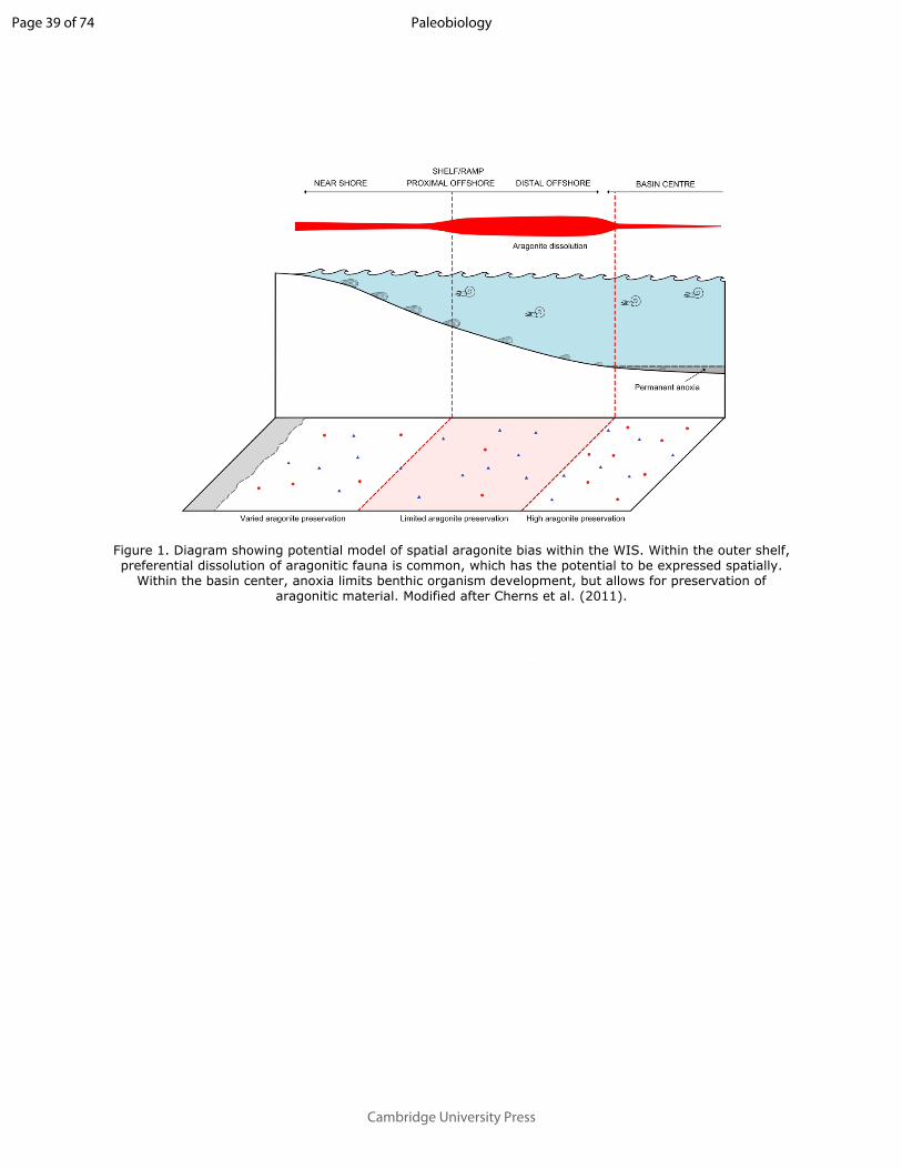
For Peer Review

Figure 1. Diagram showing potential model of spatial aragonite bias within the WIS. Within the outer shelf,

preferential dissolution of aragonitic fauna is common, which has the potential to be expressed spatially.

Within the basin center, anoxia limits benthic organism development, but allows for preservation of

aragonitic material. Modified after Cherns et al. (2011).

Page 39 of 74


Paleobiology

For Peer Review

Figure 2. Paleogeographic zoned maps of the WIS used in this study. Depth-based zones are designated as

nearshore, proximal offshore, distal offshore and basin center (Fig. 1); A. Paleobathymetric map of the

Cenomanian-Turonian; B. Paleobathymetric map of the early Campanian.

Page 40 of 74


Paleobiology

For Peer Review

Figure 3. Diagram showing potential model of apparent range size reduction due to spatially variable

aragonite preservation. Assuming that calcitic and aragonitic species of bivalve were both living at four

separate localities but aragonitic dissolution strongly influenced one of those locations (A), the resulting

convex hull for the aragonitic fauna drawn from surviving fossil occurrences would likely be smaller than

that of the calcitic organism (B).

Page 41 of 74


Paleobiology

For Peer Review

Plots of generic level M2 sampling probabilities for the Cenomanian-Turonian (A, C, E, G) and lower

Campanian (B, D, F, H) time slices across depth zones, split into carbonate and siliciclastic sampling

opportunities. All results are plotted with percentage of carbonate collections per depth zone A.

Cenomanian-Turonian generic level sampling probability, plotted with percentage of carbonate collections

per depth zone; B. lower Campanian generic level sampling probability, plotted with percentage of carbonate

collections per depth zone; C. Cenomanian-Turonian ammonite sampling probability; D. lower Campanian

ammonite sampling probability; E. Cenomanian-Turonian aragonitic bivalve sampling probability; F. lower

Campanian aragonitic bivalve sampling probability; E. Cenomanian-Turonian calcitic bivalve sampling

probability; F. lower Campanian calcitic bivalve sampling probability.

Page 42 of 74


Paleobiology

For Peer Review

Graph summarizing multiple logistic regression model results (T1-T8 = Tables 1-8). Final models are

presented within columns, whereas factors are presented along rows for those models. Results are

presented as either green (comparatively positive odds of sampling compared to reference factor), red

(comparatively negative odds of sampling compared to reference factor), light grey (factor not statistically

significant) and dark grey (factor not included in the final model). The following factors are used as a

baseline for comparison: Mineralogy = aragonite; lithology = mudstone, lithology with mineralogy =

aragonite:mudstone; zone = Basin Center (BC); diet = carnivore. Note that the magnitude of regression

coefficients is not presented within this graph. NS: Near Shore; POS: Proximal Offshore; DOS: Distal

offshore; BC: Basin Center.

Page 43 of 74


Paleobiology

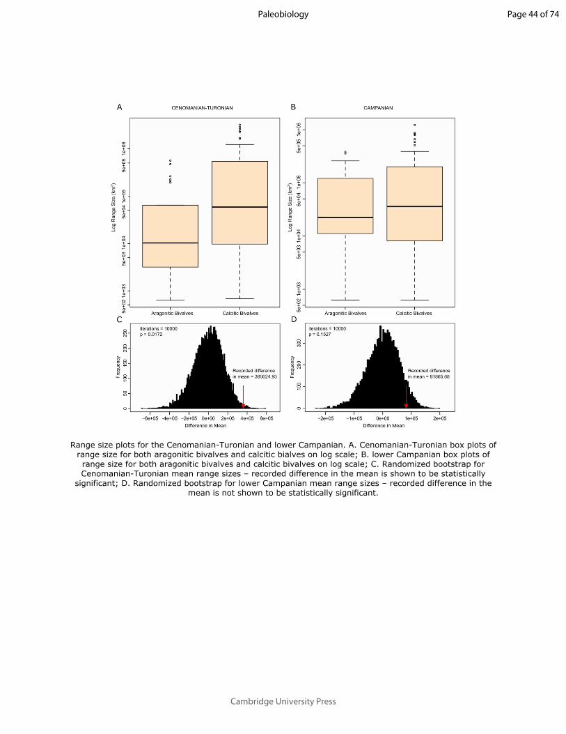
For Peer Review

Range size plots for the Cenomanian-Turonian and lower Campanian. A. Cenomanian-Turonian box plots of

range size for both aragonitic bivalves and calcitic bialves on log scale; B. lower Campanian box plots of

range size for both aragonitic bivalves and calcitic bivalves on log scale; C. Randomized bootstrap for

Cenomanian-Turonian mean range sizes – recorded difference in the mean is shown to be statistically

significant; D. Randomized bootstrap for lower Campanian mean range sizes – recorded difference in the

mean is not shown to be statistically significant.

Page 44 of 74


Paleobiology

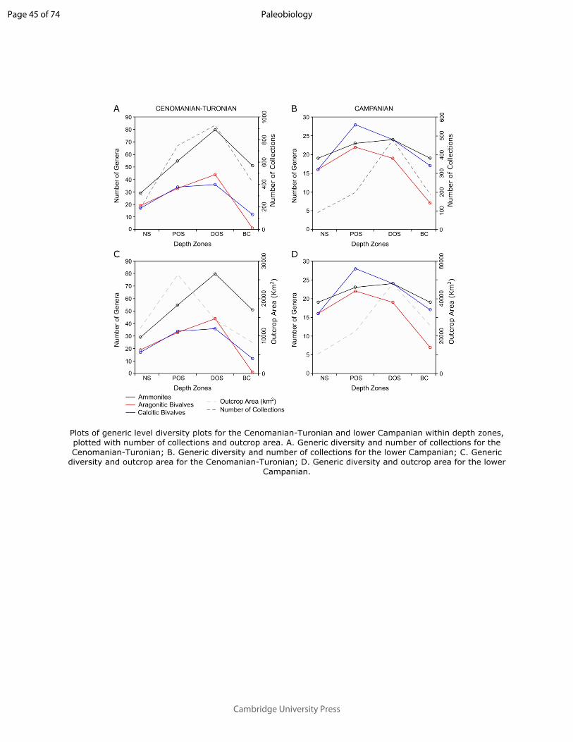
For Peer Review

Plots of generic level diversity plots for the Cenomanian-Turonian and lower Campanian within depth zones,

plotted with number of collections and outcrop area. A. Generic diversity and number of collections for the

Cenomanian-Turonian; B. Generic diversity and number of collections for the lower Campanian; C. Generic

diversity and outcrop area for the Cenomanian-Turonian; D. Generic diversity and outcrop area for the lower

Campanian.

Page 45 of 74


Paleobiology

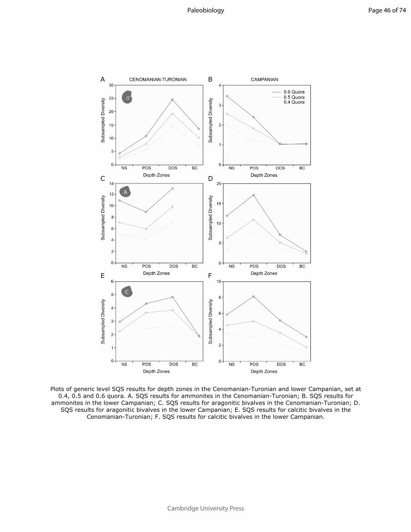
For Peer Review

Plots of generic level SQS results for depth zones in the Cenomanian-Turonian and lower Campanian, set at

0.4, 0.5 and 0.6 quora. A. SQS results for ammonites in the Cenomanian-Turonian; B. SQS results for

ammonites in the lower Campanian; C. SQS results for aragonitic bivalves in the Cenomanian-Turonian; D.

SQS results for aragonitic bivalves in the lower Campanian; E. SQS results for calcitic bivalves in the

Cenomanian-Turonian; F. SQS results for calcitic bivalves in the lower Campanian.

Page 46 of 74


Paleobiology

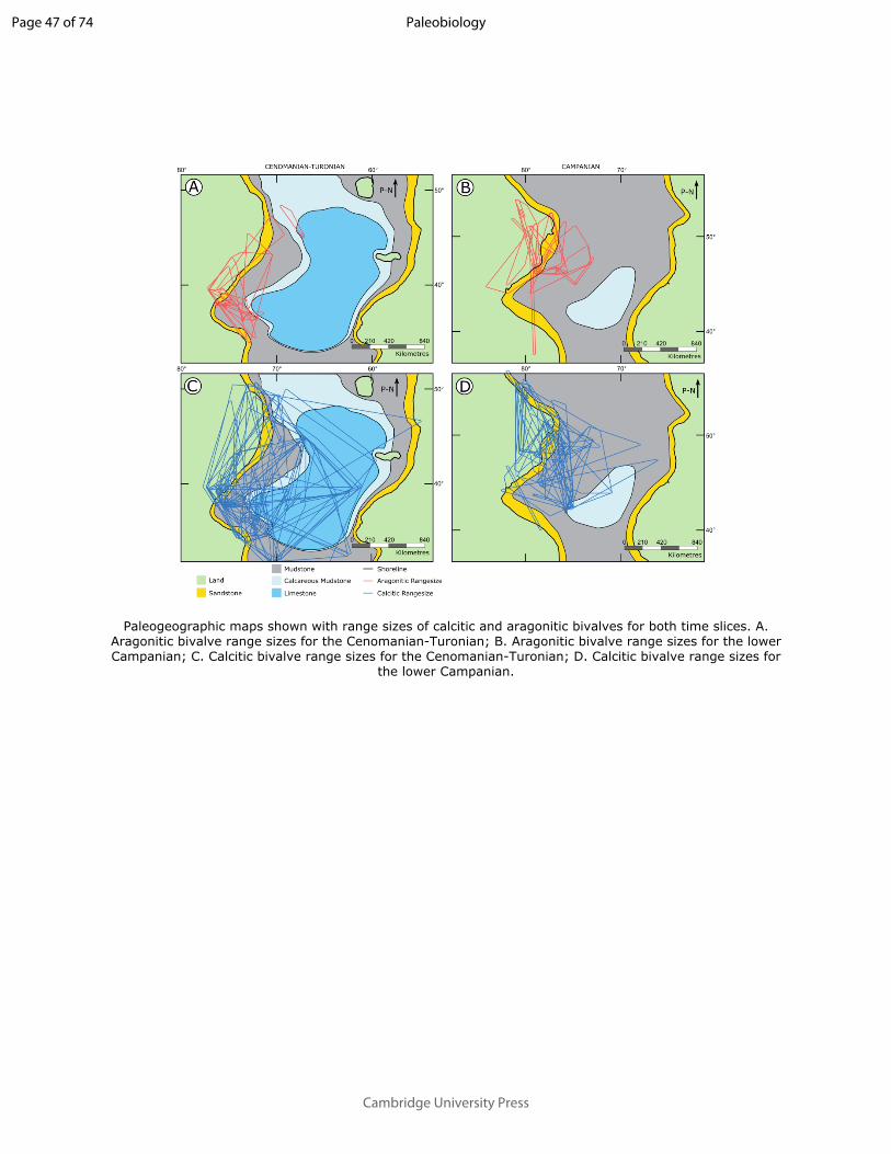
For Peer Review

Paleogeographic maps shown with range sizes of calcitic and aragonitic bivalves for both time slices. A.

Aragonitic bivalve range sizes for the Cenomanian-Turonian; B. Aragonitic bivalve range sizes for the lower

Campanian; C. Calcitic bivalve range sizes for the Cenomanian-Turonian; D. Calcitic bivalve range sizes for

the lower Campanian.

Page 47 of 74


Paleobiology

For Peer Review

Final Model AIC Factor Regression coefficient Standard errorM + D + L + Z + M:L 22367* M-Calcite 1.516 0.080

D-Chemosymbiont deposit feeder 1.353 0.239L-Sandstone 0.672 0.115L-Silt 0.759 0.362M-Calcite:L-Limestone 1.338 0.192L-Limestone -1.415 0.184DOS -0.410 0.082NS -0.754 0.114POS -0.684 0.089D-Herbivore -1.870 1.022M-Calcite:L-Calcarenite 1.146 0.611

Table for Multiple Logistic Regression results for all bivalves within the Cenomanian-Turonian across the whole seaway, using model with lowest AIC score. M - Mineralogy; D - Diet; L - Lithology; Z – depth zone.

Page 48 of 74


Paleobiology

For Peer Review

p-value< 2e-16 ***1.45e-08 ***5.39e-09 ***0.0359 * 3.35e-12 ***1.49e-14 ***6.70e-07 ***4.30e-11 ***1.10e-14 *** 0.0673 . 0.0605 .

Table for Multiple Logistic Regression results for all bivalves within the Cenomanian-Turonian across the whole seaway, using model with lowest AIC score. M - Mineralogy; D - Diet; L - Lithology; Z – depth zone.

Page 49 of 74


Paleobiology

For Peer Review

Page 50 of 74


Paleobiology

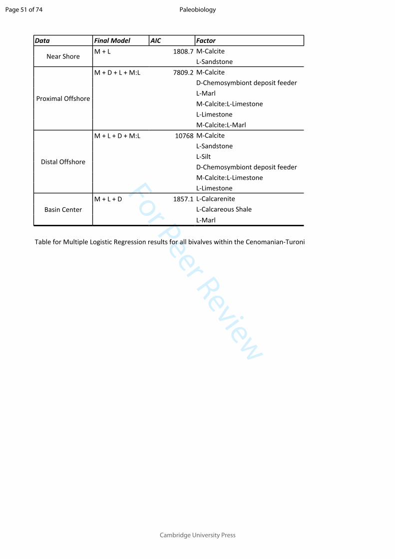
For Peer Review

Data Final Model AIC Factor

Near ShoreM + L 1808.7 M-Calcite

L-Sandstone

Proximal Offshore

M + D + L + M:L 7809.2 M-CalciteD-Chemosymbiont deposit feederL-MarlM-Calcite:L-LimestoneL-LimestoneM-Calcite:L-Marl

Distal Offshore

M + L + D + M:L 10768 M-CalciteL-SandstoneL-SiltD-Chemosymbiont deposit feederM-Calcite:L-LimestoneL-Limestone

Basin CenterM + L + D 1857.1 L-Calcarenite

L-Calcareous ShaleL-Marl

Table for Multiple Logistic Regression results for all bivalves within the Cenomanian-Turonian for each depth zone, using models with lowest AIC scores. M - Mineralogy; D - Diet; L – Lithology.

Page 51 of 74


Paleobiology

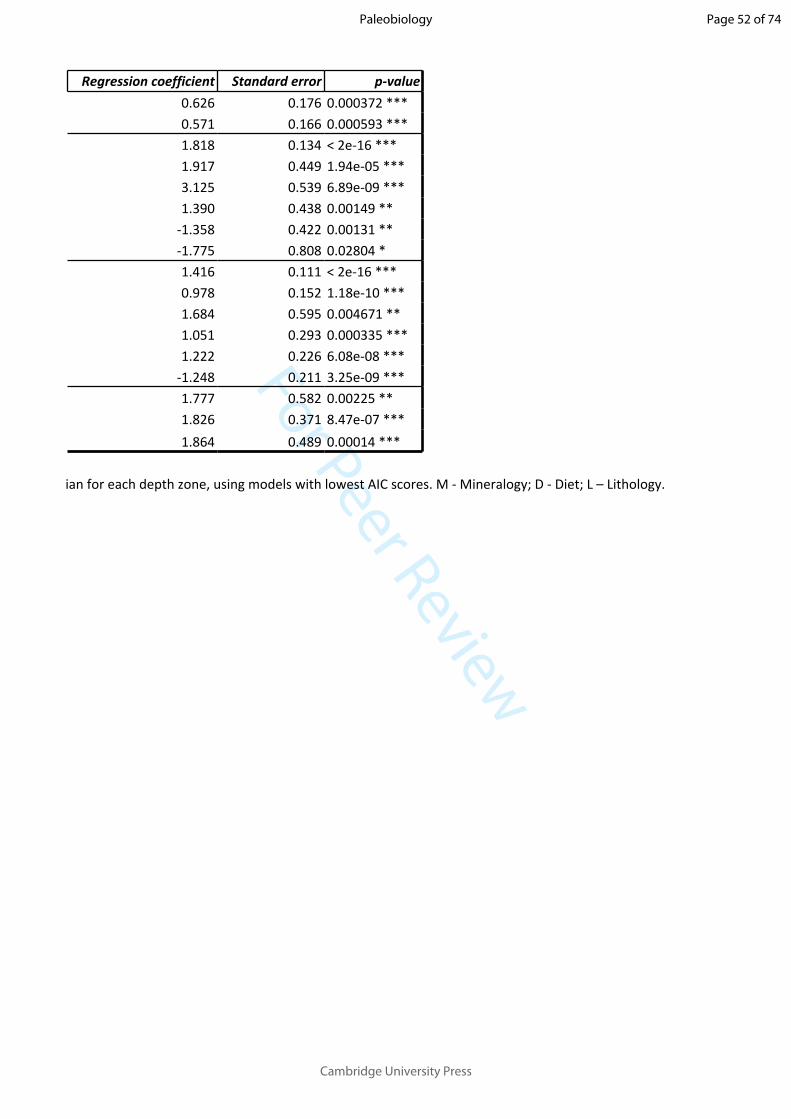
For Peer Review

Regression coefficient Standard error p-value0.626 0.176 0.000372 ***0.571 0.166 0.000593 ***1.818 0.134 < 2e-16 ***1.917 0.449 1.94e-05 ***3.125 0.539 6.89e-09 ***1.390 0.438 0.00149 **

-1.358 0.422 0.00131 ** -1.775 0.808 0.02804 *1.416 0.111 < 2e-16 ***0.978 0.152 1.18e-10 ***1.684 0.595 0.004671 ** 1.051 0.293 0.000335 ***1.222 0.226 6.08e-08 ***

-1.248 0.211 3.25e-09 ***1.777 0.582 0.00225 ** 1.826 0.371 8.47e-07 ***1.864 0.489 0.00014 ***

Table for Multiple Logistic Regression results for all bivalves within the Cenomanian-Turonian for each depth zone, using models with lowest AIC scores. M - Mineralogy; D - Diet; L – Lithology.

Page 52 of 74


Paleobiology

For Peer Review

Page 53 of 74


Paleobiology

For Peer Review

Final Model AIC Factor Regression coefficient Standard errorM + Z + L + M:L 46464* M-Calcite 0.741 0.044

L-Conglomerate 1.495 0.324L-Marl 0.593 0.174M-Calcite:L-Calcarenite 1.269 0.319M-Calcite:L-Calcareous Shale 2.290 0.280M-Calcite:L-Limestone 0.202 0.072M-Calcite:L-Sandstone 0.595 0.095DOS -0.530 0.050NS -0.700 0.076POS -0.755 0.056L-Calcarenite -0.959 0.260L-Calcareous Shale -1.561 0.253L-Limestone -0.288 0.050L-Sandstone -0.152 0.067M-Calcite:L-Conglomerate -1.857 1.057

Table for Multiple Logistic Regression for all organisms (including ammonites) within the Cenomanian-Turonian across the whole seaway, using model with lowest AIC score. M - Mineralogy; L - Lithology; Z – depth zone.

Page 54 of 74


Paleobiology

For Peer Review

p-value< 2e-16 ***3.92e-06 ***0.000654 ***7.10e-05 ***3.03e-16 ***0.004996 ** 4.31e-10 ***< 2e-16 ***< 2e-16 ***< 2e-16 ***0.000227 ***6.77e-10 ***6.82e-09 ***0.024007 * 0.079016 .


Page 55 of 74


Paleobiology

For Peer Review


Page 56 of 74


Paleobiology

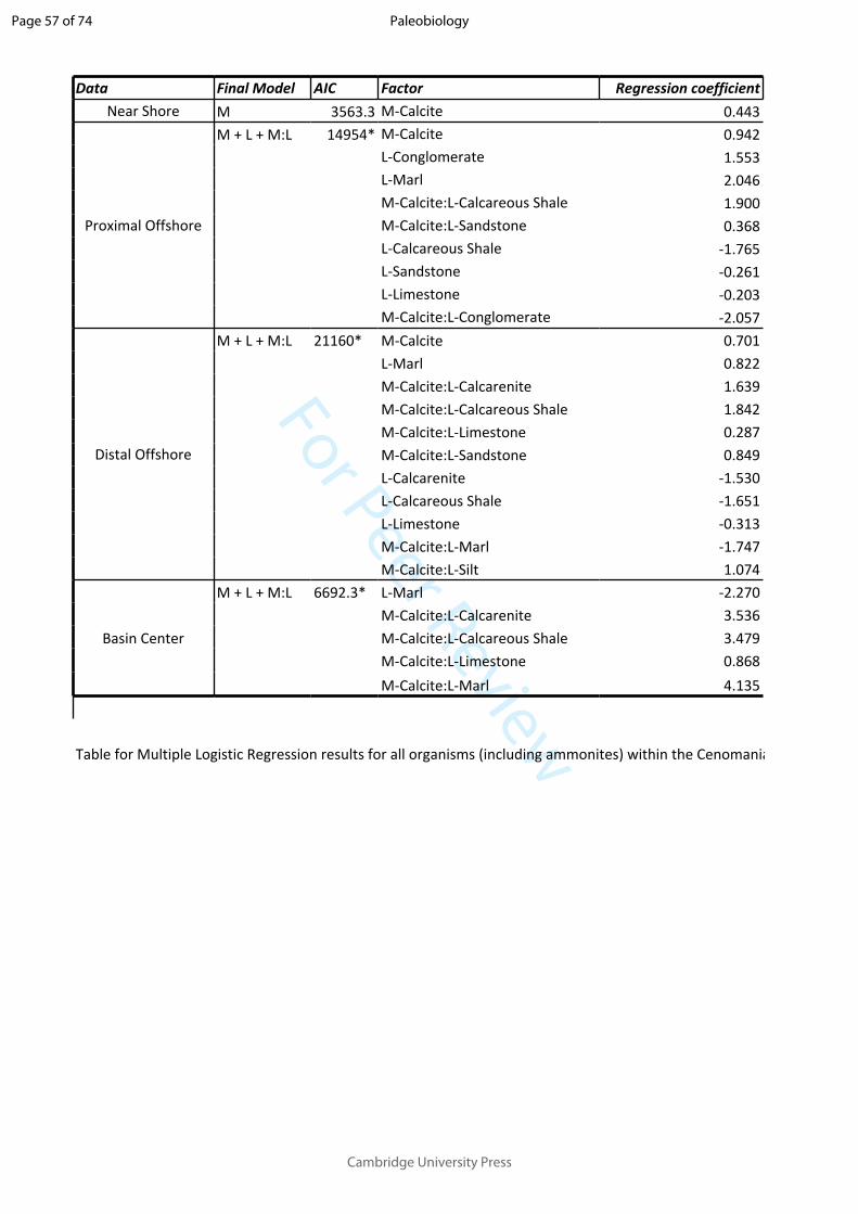
For Peer Review

Data Final Model AIC Factor Regression coefficientNear Shore M 3563.3 M-Calcite 0.443

Proximal Offshore

M + L + M:L 14954* M-Calcite 0.942L-Conglomerate 1.553L-Marl 2.046M-Calcite:L-Calcareous Shale 1.900M-Calcite:L-Sandstone 0.368L-Calcareous Shale -1.765L-Sandstone -0.261L-Limestone -0.203M-Calcite:L-Conglomerate -2.057

Distal Offshore

M + L + M:L 21160* M-Calcite 0.701L-Marl 0.822M-Calcite:L-Calcarenite 1.639M-Calcite:L-Calcareous Shale 1.842M-Calcite:L-Limestone 0.287M-Calcite:L-Sandstone 0.849L-Calcarenite -1.530L-Calcareous Shale -1.651L-Limestone -0.313M-Calcite:L-Marl -1.747M-Calcite:L-Silt 1.074

Basin Center

M + L + M:L 6692.3* L-Marl -2.270M-Calcite:L-Calcarenite 3.536M-Calcite:L-Calcareous Shale 3.479M-Calcite:L-Limestone 0.868M-Calcite:L-Marl 4.135

Table for Multiple Logistic Regression results for all organisms (including ammonites) within the Cenomanian-Turonian for each depth zone, using models with lowest AIC scores. M - Mineralogy; L – Lithology.

Page 57 of 74


Paleobiology

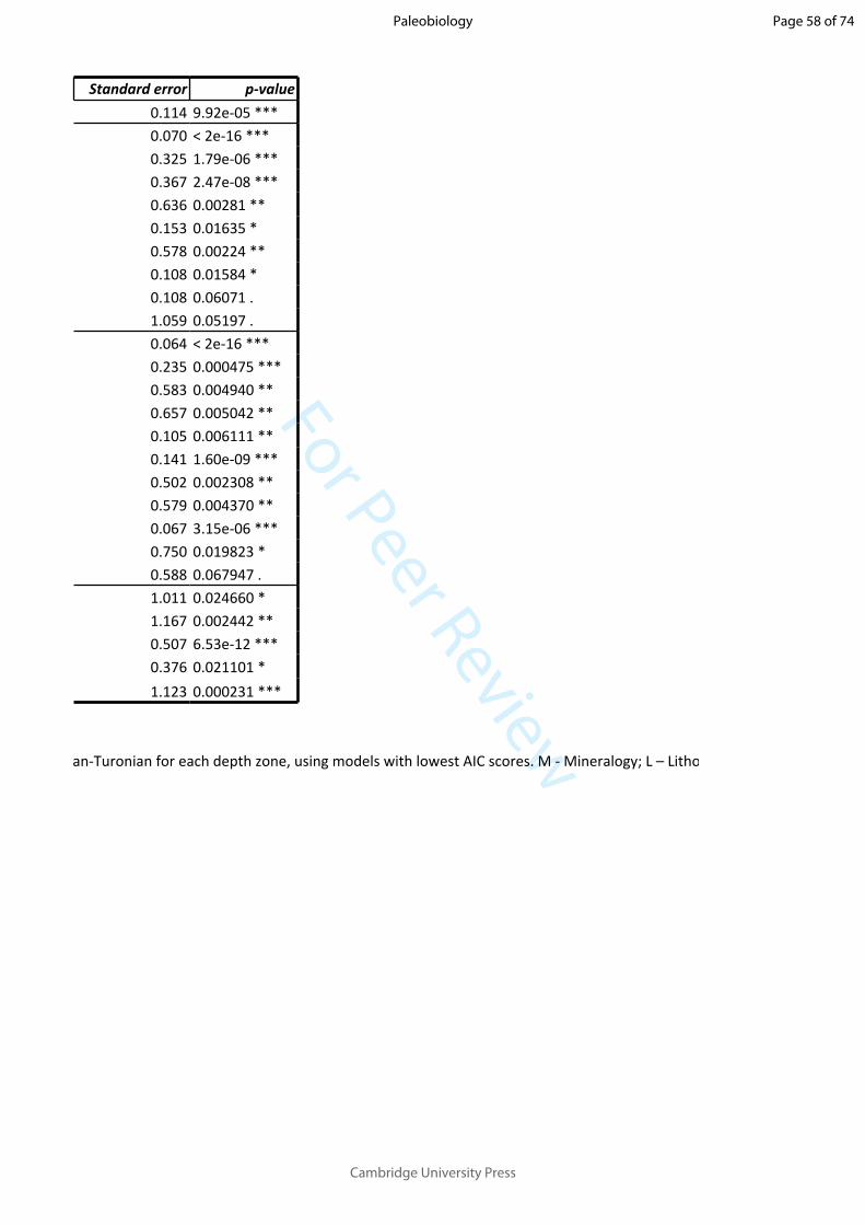
For Peer Review

Standard error p-value0.114 9.92e-05 ***0.070 < 2e-16 ***0.325 1.79e-06 ***0.367 2.47e-08 ***0.636 0.00281 ** 0.153 0.01635 * 0.578 0.00224 ** 0.108 0.01584 * 0.108 0.06071 . 1.059 0.05197 . 0.064 < 2e-16 ***0.235 0.000475 ***0.583 0.004940 ** 0.657 0.005042 ** 0.105 0.006111 ** 0.141 1.60e-09 ***0.502 0.002308 ** 0.579 0.004370 ** 0.067 3.15e-06 ***0.750 0.019823 * 0.588 0.067947 . 1.011 0.024660 * 1.167 0.002442 ** 0.507 6.53e-12 ***0.376 0.021101 * 1.123 0.000231 ***

Table for Multiple Logistic Regression results for all organisms (including ammonites) within the Cenomanian-Turonian for each depth zone, using models with lowest AIC scores. M - Mineralogy; L – Lithology.

Page 58 of 74


Paleobiology

For Peer ReviewTable for Multiple Logistic Regression results for all organisms (including ammonites) within the Cenomanian-Turonian for each depth zone, using models with lowest AIC scores. M - Mineralogy; L – Lithology.

Page 59 of 74


Paleobiology

For Peer Review

Final Model AIC Factor Regression coefficient Standard errorM + L + M:L 7063.9* M-Calcite 0.767 0.115

L-Sandstone 0.594 0.168M-Calcite:L-Limestone 1.292 0.538M-Calcite:L-Sandstone -0.496 0.209M-Calcite:L-Siltstone 1.838 1.044

Table for Multiple Logistic Regression results for all bivalves within the lower Campanian across the whole seaway, using model with lowest AIC score. M - Mineralogy; D - Diet; L - Lithology; Z – depth zone.

Page 60 of 74


Paleobiology

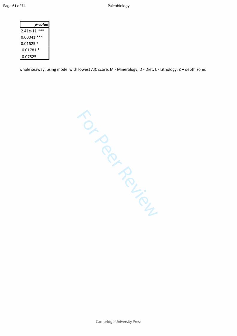
For Peer Review

p-value2.41e-11 ***0.00041 ***0.01625 * 0.01781 * 0.07825 .

Table for Multiple Logistic Regression results for all bivalves within the lower Campanian across the whole seaway, using model with lowest AIC score. M - Mineralogy; D - Diet; L - Lithology; Z – depth zone.

Page 61 of 74


Paleobiology

For Peer Review

Page 62 of 74


Paleobiology

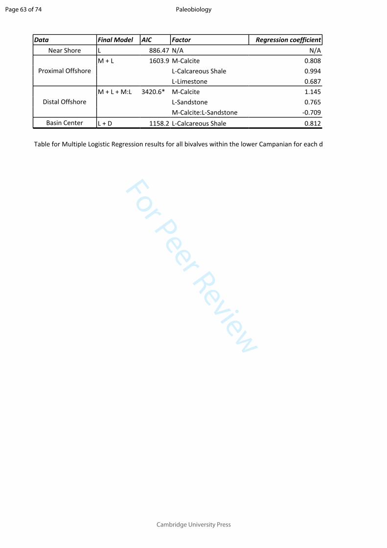
For Peer Review

Data Final Model AIC Factor Regression coefficientNear Shore L 886.47 N/A N/A

Proximal OffshoreM + L 1603.9 M-Calcite 0.808

L-Calcareous Shale 0.994L-Limestone 0.687

Distal OffshoreM + L + M:L 3420.6* M-Calcite 1.145

L-Sandstone 0.765M-Calcite:L-Sandstone -0.709

Basin Center L + D 1158.2 L-Calcareous Shale 0.812

Table for Multiple Logistic Regression results for all bivalves within the lower Campanian for each depth zone, using models with lowest AIC scores. M - Mineralogy; D - Diet; L - Lithology; Z – depth zone.

Page 63 of 74


Paleobiology

For Peer Review

Standard error p-valueN/A N/A

0.184 1.08e-05 ***0.467 0.03336 * 0.247 0.00545 ** 0.169 1.41e-11 ***0.260 0.00332 ** 0.322 0.02768 * 0.222 0.000259 ***

Table for Multiple Logistic Regression results for all bivalves within the lower Campanian for each depth zone, using models with lowest AIC scores. M - Mineralogy; D - Diet; L - Lithology; Z – depth zone.

Page 64 of 74


Paleobiology

For Peer ReviewTable for Multiple Logistic Regression results for all bivalves within the lower Campanian for each depth zone, using models with lowest AIC scores. M - Mineralogy; D - Diet; L - Lithology; Z – depth zone.

Page 65 of 74


Paleobiology

For Peer Review

Final Model AIC Factor Regression coefficient Standard error p-valueZ + M 16712 DOS -0.323 0.067 1.61e-06 ***

NS -0.203 0.095 0.033311 * POS -0.281 0.078 0.000307 ***M-Calcite -0.146 0.054 0.006599 **

Table for Multiple Logistic Regression results for all organisms (including ammonites) within the lower Campanian across the whole seaway, using model with lowest AIC score. M - Mineralogy; L - Lithology; Z – depth zone.

Page 66 of 74


Paleobiology

For Peer Review


Page 67 of 74


Paleobiology

For Peer Review


Page 68 of 74


Paleobiology

For Peer Review

Data Final Model AIC Factor Regression coefficient Standard errorNear Shore Rcoll ~ 1 1747.1 N/A N/A N/A

Proximal Offshore M 3683 M-Calcite -0.307 0.117Distal Offshore Rcoll ~ 1 8319.3 N/A N/A N/A

Basin Center L + M + L:M 1151.9* N/A N/A N/A

Table for Multiple Logistic Regression results for all organisms (including ammonites) within the lower Campanian for each depth zone, using models with lowest AIC scores. M - Mineralogy; L – Lithology.

Page 69 of 74


Paleobiology

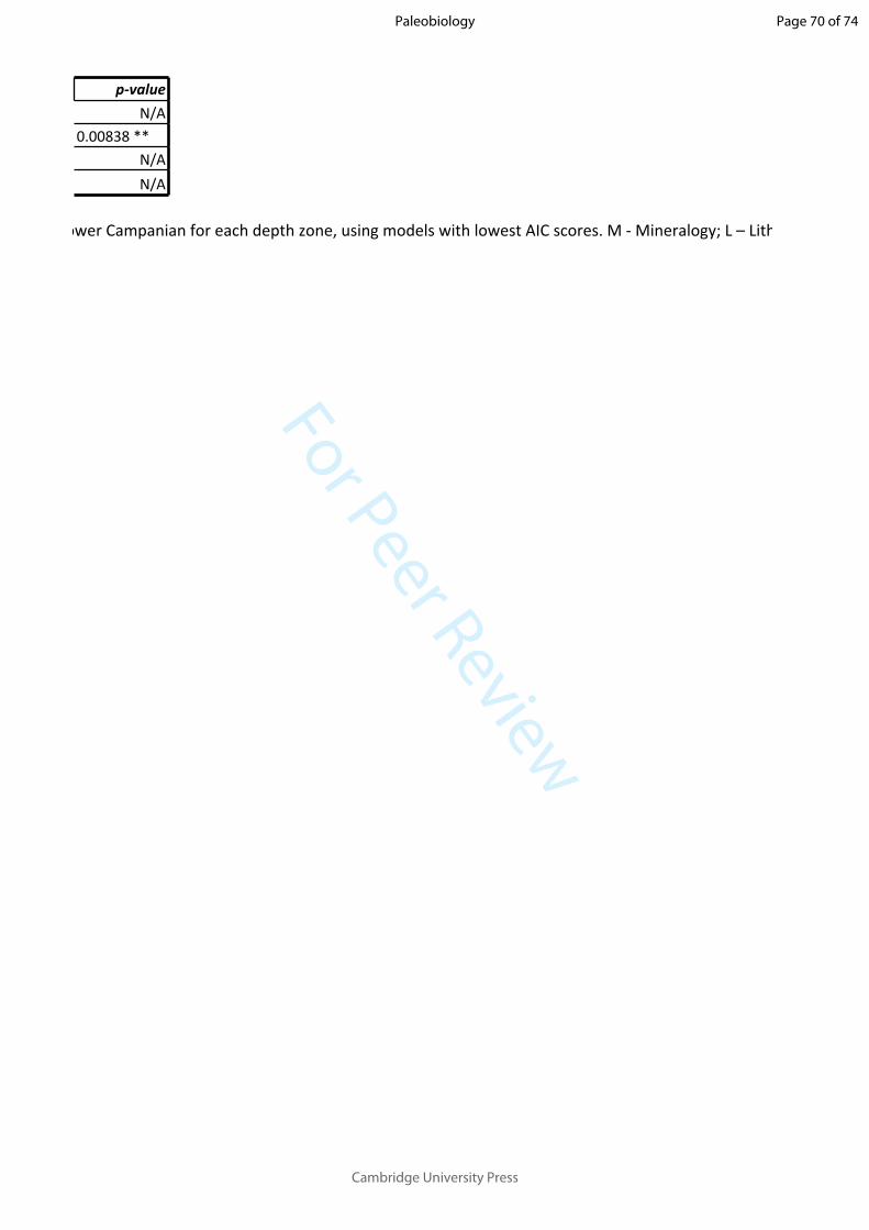
For Peer Review

p-valueN/A

0.00838 ** N/AN/A


Page 70 of 74


Paleobiology

For Peer Review


Page 71 of 74


Paleobiology

For Peer Review

DISTANCE CorrelationSpearman's

RhoCE

NO

MAN

IAN

-TU

RON

IAN AMMONITES

Outcrop AreaAmmonite occurrences vs. Outcrop Area 0.475Ammonite raw diversity vs. Outcrop Area 0.704

CollectionsAmmonite occurrences vs. Collections 0.885Ammonite raw diversity vs. Collections 0.732

ARAG. BIVALVESOutcrop Area

Aragonitic bivalve occurrences vs. Outcrop Area 0.634Aragonitic bivalve raw diversity vs. Outcrop Area 0.640

CollectionsAragonitic bivalve occurrences vs. Collections 0.568Aragonitic bivalve raw diversity vs. Collections 0.502

CALC. BIVALVESOutcrop Area

Calcitic bivalve occurrences vs. Outcrop Area 0.534Calcitic bivalve raw diversity vs. Outcrop Area 0.678

CollectionsCalcitic bivalve occurrences vs. Collections 0.904Calcitic bivalve raw diversity vs. Collections 0.738

LOW

ER C

AMPA

NIA

N

AMMONITESOutcrop Area

Ammonite occurrences vs. Outcrop Area 0.221Ammonite raw diversity vs. Outcrop Area 0.343

CollectionsAmmonite occurrences vs. Collections 0.970Ammonite raw diversity vs. Collections 0.727

ARAG. BIVALVESOutcrop Area

Aragonitic bivalve occurrences vs. Outcrop Area 0.473Aragonitic bivalve raw diversity vs. Outcrop Area 0.404

CollectionsAragonitic bivalve occurrences vs. Collections 0.822Aragonitic bivalve raw diversity vs. Collections 0.759

CALC. BIVALVESOutcrop Area

Calcitic bivalve occurrences vs. Outcrop Area 0.056Calcitic bivalve raw diversity vs. Outcrop Area 0.322

CollectionsCalcitic bivalve occurrences vs. Collections 0.958Calcitic bivalve raw diversity vs. Collections 0.879

Table 9: Spearman’s rank correlations between generic diversity of faunal groups and various sampling proxies for distance-from-paleoshoreline zones within the Cenomanian-Turonian and lower Campanian

Page 72 of 74


Paleobiology

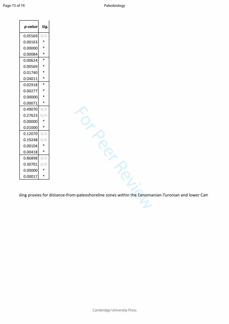
For Peer Review

p-value Sig.

0.05569 N/A0.00163 *0.00000 *0.00084 *0.00624 *0.00569 *0.01740 *0.04011 *0.02918 *0.00277 *0.00000 *0.00071 *0.49070 N/A0.27623 N/A0.00000 *0.01000 *0.12070 N/A0.19248 N/A0.00104 *0.00418 *0.86898 N/A0.30701 N/A0.00000 *0.00017 *

Table 9: Spearman’s rank correlations between generic diversity of faunal groups and various sampling proxies for distance-from-paleoshoreline zones within the Cenomanian-Turonian and lower Campanian

Page 73 of 74


Paleobiology

For Peer ReviewTable 9: Spearman’s rank correlations between generic diversity of faunal groups and various sampling proxies for distance-from-paleoshoreline zones within the Cenomanian-Turonian and lower Campanian

Page 74 of 74


Paleobiology

Documents

Aragonite bias exhibits systematic spatial variation in