WATER RESOURCES BULLETIN VOL. 12, NO. 5 AMERICAN WATER RESOURCES ASSOCIATION OCTOBER 1976

AQUIFER MANAGEMENT UNDER TRANSIENT AND STEADY -STATE CONDITIONS'

William M. Alley, Eduardo Aguado, and Irwin Rernson2

ABSTRACT: The equations of transient and steady-state flow in two-dimensional artesian aquifers are approximated using finite differences. The resulting linear difference equations, combined with other linear physical and management constraints and a linear objective function, comprise a linear programming (LP) formulation. Solutions of such LP modcls arc used to determine optimal well distributions and pumping rates to meet given management objectives for a hypothetical transient problem and for a steady-state field problem. ( K L Y TERMS: aquifers; finite differences; groundwater management; linear programming; optimization.)

INTRODUCTION The determination of optimum aquifer management schemes is becoming increasingly

important. For example, one might desire the optimum pumping distribution that will achieve a specified total discharge rate while maintaining prescribed groundwater heads. An alternate management objective might be to minimize the discharge rate required to lower aquifer heads to specified levels or t o reverse the hydraulic gradient along a line of wells.

For most ground water management schemes, the ground water hydraulics should be included in the decision-making process. Aguado and Remson (1974) included ground water variables as decision variables by using finite difference approximations of the governing differential equations as constraints in linear programming (LP) management models. The technique was then used to determine an optimum dewatering scheme for a large excavation (Aguado, et al., 1974). The LP models were tested and verified for a steady-state, two-dimensional, artesian problem using numerical and electrical analog ground water models (Remson, et al., 1974). Finally, finite element approximations were substituted for the finite difference approximations in a similar LP model (Sitar, 1975).

The inclusion of ground water variables directly as decision variables in LP management models has thus far been used for steady-state one- and two-dimensional

'Paper No. 76051 of the WaterResources Bulletiir. Discussions are open until June 1,1977. Respcctively, Research Assistant, Department of Applied Earth Sciences; Rescarch Assistant,

Department of Geology; and Professor of Applied Earth Scicnces and Geology; all of Stanl'ord University, Stanford, California 94305.

963

964 Alley, Aguado, and Remson

problems and for transient one-dimensional problems. It is the purpose of this paper to extend the method to two-dimensional transient situations, illustrating the use with a hypothetical example. In addition, the steady-state method is applied to a two- dimensional waste-disposal field problem.

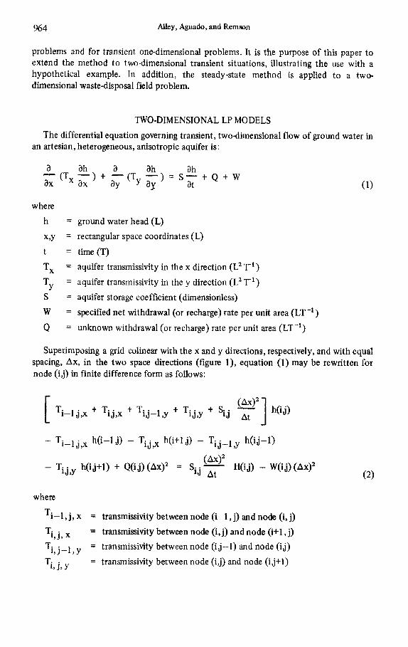
TWO-DIMENSIONAL LP MODELS The differential equation governing transient, two-dimensional flow of ground water in

an artesian, heterogeneous, anisotropic aquifer is:

a ah a ah ah - (Tx a,) t (T - ) = S - + Q + w ax aY at

where h

x,y t = time(T)

Tx

Ty S

W Q

= ground water head (L) = rectangular space coordinates (L)

= aquifer transmissivity in the x direction (L' T') = aquifer transmissivity in the y direction (L2 T') = aquifer storage coefficient (dimensionless) = specified net withdrawal (or recharge) rate per unit area (LT-')

= unknown withdrawal (or recharge) rate per unit area (LT-')

Superimposing a grid colinear with the x and y directions, respectively, and with equal spacing, Ax, in the two space directions (figure I ) , equation (1) may be rewritten for node (ij) in finite difference form as follows:

- Ti-lj,x h(i-lj) - Tij,x h(it1j) - Tij-l,y h(ij-1)

(Ax)' - Tij,y h(ijt1) + Q(ij)(Ax)' = S . - H(ij) - W(ij)(Ax)*

At

where

Ti-1, j, x = transmissivity between node (i-1 , j) and node (i, j)

Ti, j , x = transmissivity between node (i, j) and node (i+l , j)

Ti,j-l ,y = transmissivity between node (ij-1) and node (ij) = transmissivity between node (i j) and node (i j+l) Ti, j, Y

96 5 Aquifer Managcrncnt

J S Y

Figure 1. Computational Star and Definition of Transmissivities.

= storage coefficient at node (ij) Si, j Ax = constant grid spacing in x and y directions

At = time interval h(i, j), h(i-1, j), h(i+l, j), h(i, j-l), h(i, j+l)

H(i, j)

= unknown hydraulic heads at the indicated nodes at the end of the time interval being considered

= known hydraulic head at node (ij) at the beginning of the time interval being considered. (This is known from the solution obtained for the previous time interval or from the initial conditions at the beginning of the simulation.)

= unknown volumetric withdrawal (or recharge) rate per unit area at node

= specified net volumetric withdrawal (or recharge) rate per unit area at node (ij). For example, this might include ground water recharge due to infiltrated precipitation

Q(i, j)

W(i, j) ( i d

Alley, Aguado, and Remson 966

Equation, (2) has six unknowns, the hydraulic heads at the five nodes (ij), (i-1 j ) , (i+l,j), (i,j-1), (i,ji-l), and the withdrawal (or recharge) rate Q(ij) at node (id). The withdrawal (or recharge) rate Q(ij) will be determined by the optimization procedure. The actual withdrawal (or recharge) rate at node (ij) will be the algebraic sum of the pre-specified rate, W(ij), and the rate to be determined, Q(i,j).

Equation (2) is written for every node in the problem domain. The resulting equations combined with other linear constraints and with a linear objective function form a problem well suited to linear programming. The LP solution consists of the values of Q(ij) that achieve the specified management objective and the resulting values of h(ij). At nodes where Q(i,j) is zero in the solution, no pumping is required and no wells should be installed.

The steady-state equivalent of equation (1) is obtained by setting S -equal to ~ $ 0 .

For steady-state conditions, equation (2) is changed only in that the fac or S i,j is set equal to zero.

ah

All LP solutions were obtained using the IBM MPS/360 code.

APPLICATION TO A TRANSIENT PROBLEM

Figure 2 shows initial and boundary heads in a hypothetical aquifer on which a square grid has been superimposed. Constant heads are maintained at all boundary nodes. The optimal well distribution and pumping rates for each of 20 days are desired. Pumped wells may be located at any interior nodes.

Fifteen thousand gallons per day (gpd) are required for the first 10 days. At least 5000 gpd during this period must come from a well at node (4,4). The heads at the interior nodes must not fall below the values specified by the inequalities (3d). The objective is to pump at the above total rate while meeting the above constraints and maintaining the sum of the ground water heads in the aquifer at a maximum. Choosing a At of 5 days, the 10-day interval is simulated in two LP steps.

For days 11 through 15, the same constraints and objectives are specified except that the required total pumping rate is increased to 30,000 gpd.

Finally, for days 16 through 20, the objective is changed to maximization of the total withdrawal rate while continuing to maintain the same lower limits for the heads at the interior nodes and restricting discharge to nodes (2,2), (2,4), (4,4), and (5,3).

For the first time interval (days 1 through 5), the LP formulation is:

5 4 Maximize z = X X h(i,j)

i=2 j=2

5 4

i=2 j=2 tributary to all the selected subject to: C X Q(i,j) = 1.4 x feet per day over the area

nodes (1 5,000 gpd) (3b)

Q(4,4) > 4.64 x feet per day over the area tributary to node (4,4) (5000 gpd) (3c)

Aquifer Managemcnt 96 7

h(2, j) 2 1.50 f t ; j=2,3,4 h(3 , j ) 2 2.25 f t ; j=2,3,4 h(4,j) 2 3 . 0 0 f t ; j=2,3,4 h(5, j ) > 3.75 f t ; j=2,3,4

Equation (3a) is the objective function. Equations (3b) and (3c) are the pumping constraints. Equations ( 3 4 are the constraints specifying the lower limits allowed for the ground water heads at the end of the time interval. Equations (3e) in figure 3 are the

i = l i = 2 i = 3 1=4 1=5 i = 6

j = 1

j = 2

j = 3

j = 4

j = 5

Y

1

1

1

4 4

4 4

- 2 1 4 14

Figure 2. Initial Heads and Constant-Head Boundary Conditions for the Transient Two-Dimensional Problem. Ground Water Heads arc in Fcct

The Physical Parameters are:

T ~ J , ~ = T ~ J , ~ = 1337 ft2 per day (10,000 gpd/ft) for i=1,2,3,4

Tij,x = T ~ J , ~ = 668 f t2 per day (5000 gpd/ft) for i=5,6

Sij = 0.001 at aU intcrior nodes

A x = 1200ft

A t = 5 days

Wi,i = 0 at all nodes

5636

-1

337

0 -1

337

5636

-1

337

0 -1

337

5636

-1

337

0 0

0 -1

337

0 0

0 -1

337

0 0

0 0

0 0

0 0

0 0

0 0

0 0

0 0

0 0

+144

0000

-133

7 0 0 56

36

-133

7 0 -1

337

0 0 0 0 0

5163

65

00

1152

65

00

8500

5

160

8500

0 0 -1

337

56

36

-133

7 0 -1

337

0 0 0 0

-133

7 0 0

-133

7 0 -1

337

56

36

0 0 -1

337 0 0 0

0 0 0 -1

337 0 0

5636

-1

137 0

-1 3

37

0 0

0 0 0 0 -1

337

0

5636

-1

337

0

-133

7 0

-133

7

0 0 0 0 0 -1

337

0

-133

7 56

36

0 0 -1

337

0 0

0 0

0 0

0 0

0 0

0 0

-133

7 0

0 -1

337

0 0

3629

- 6

68

- 66

8 36

29

0 - 6

68

0 0 -1

337 0

-

668

3629

8 EL 0 e, Ja 6 8

Figu

re 3

. M

atrix

of

Nod

e E

quat

ions

for

the

Tra

nsie

nt T

wo-

Dim

ensi

onal

Pro

blem

for

the

Fir

st 5

-Day

T

ime

Inte

rval

. The

Fix

ed H

ydra

ulic

Hea

ds a

t th

e B

ound

ary

Nod

es a

nd t

he In

itial

Con

ditio

ns D

o Not

App

ear

in t

he V

ecto

r of

Unk

now

n h(

iJ)’

s; T

heir

Kno

wn

Con

stan

t V

alue

s ar

e Pa

rt of

the

Vec

tor

of

Rig

ht-H

and

Side

s.

Aquifer Management 969

constraint equations in unknowns h and Q generated from equation (2). They complete the LP formulation.

For the first time interval (days 1 through 5), the model chose a rate of 5000 gpd from the well at node (4,4) (table 1). This is the minimum allowable pumping rate at that node. The model assigns the remaining 10,000 gpd to one well at either node (2,4) or node (2,2). These are the nodes adjacent t o constant-head boundaries and in the part of the domain where transmissivity is greatest. Thus, wells at these nodes would discharge with minimum drawdown.

The LP formulation for the second interval (days 6 through 10) differed from that for the first interval only in the values of H(i,j), the heads at the beginning of the interval. The optimal well distribution and pumping rates for days 6 through 10 proved to be the same as for the fiist 5 days (table 1).

For days 11 through 15, the LPmodel again assigns the minimum allowable discharge, 5000 gpd to the well at node (4,4) (table 1). Of the remaining 25,000 gpd required, 15,082 gpd come from node (2,2) and the remaining 9918 gpd from node (2,4). For the interval from day 16 through day 20, the objective function was changed to maximize the discharge, and the constraints were changed to restrict discharge to nodes (2,2), (2,4), (4,4), and (5,3). The solution for this final time period is displayed in table 1.

While not displayed herein, the resulting heads at all internal nodes are part of the LP solution.

Here, we find the optimal solution for each 5-day interval from a separate LP problem. The solution is then used to specify initial conditions for the next 5-day interval. Because they have the same objective function, the first three Sday intervals could have been expressed using a single LP formulation as shown by Aguado and Remson (1974) for a one-dimensional problem. However, the objective function is changed for the fourth 5-day interval and this could not be combined into the single LP formulation.

To verify the LP results, the optimal pumping rates of the successive solutions were used as inputs to a ground water model solved using the computer code of Prickett and Lonnquist (1971). In all cases, the resulting heads were the same as those in the LP solutions.

TABLE 1. Optimal Pumping Rates for Transient, Two-Dimensional Problems.

PUMPING RATE b d )

Node 0-5 days 6-10 days 11-15 days 16-20 days

(2,2) (2,4) 0

15,082 12,891

9,918 11,781

5,000 2 0 s 20

10,000 * 10,000

0

5,000 (4,4) 5,000

(5 $3) 0

All other 0 nodes

0

0

0 12,956

0 0

* Alternate possibility is 10,000 gpd a t node (2,4) and 0 a t node (2,2).

970 Alley, Aguado, and Remson

APPLICATION TO A STEADY-STATE PROBLEM

With the above methodology, there is no basic difference between a transient problem and a steady-state problem. We have seen that the transient problem is solved using a series of LP models, one for each time interval. The steady-state case is solved as a single

LF’ problem, using the modified form of equation ( 2 ) , setting S. - (Ax)’ equal to zero.

The LP technique was used to study the feasibility of disposing of wastewater by injection into an aquifer system in the eastern part of Tooele Valley (figure 4), about 30 miles southwest of Salt Lake City, Utah. The area is a large, alluvial fan, and the hydrogeology is described by Gates (1 965).

Approximately 9 million gpd for two years and 2 million gpd thereafter were to be injected into the alluvial sediments at the site shown in figure 4. The recharged water must be kept from mixing with the municipal and domestic supplies at the towns of Tooele and Erda.

Before applying the optimization procedures, the aquifer system was studied with the aid of a steady-state digital model using the computer code of Pinder (1970). Although the southern two-fifths of the aquifer system in figure 4 are unconfined, the great thickness of saturated sediment allowed us to treat the entire system as confined. Recharge in the amount of 100,000 acre feet per year was applied to the model at the nodes where intermittent streams flowing from the mountains to the south and east infiltrate the alluvial fan. An equal amount of discharge is lost to springs, by evapotranspiration by phreatophytes, and by seepage to Great Salt Lake to the north.

Values of transmissivity were estimated from available data, and the model was used to generate water levels. Successive adjustments of transmissivity were made until the water levels generated by the model were in agreement with the historical water levels. Transmissivity values were found to vary from about 700,000 gallons per day per foot in the southeast to about 200,000 gallons per day per foot in the north.

The ground water model revealed also that the recharged water would bypass Tooele but would reach Erda and neighboring communities unless remedial action were taken.

It had been suggested that wells along an east-west line between the recharging site and Erda (figure 4) could be pumped at a sufficiently high rate to reverse the hydraulic gradient and prevent wastewater from reaching Erda. The pumped water would be suitable for irrigation, and a demand existed for 5 to 6 million gallons per day. The feasibility of this solution was tested using the LP steady-state technique.

The objective was to minimize total pumping from the 2 lines of wells shown in figure 4. The ground water constraint equations together with the constant-head boundary conditions were formulated as described above. The transmissivity values mentioned above were incorporated. Specified recharge and discharge rates were the W(i,j)’s. Finally, to insure reversal of the hydraulic gradient, addi’tional constraint equations specified that heads increase to the north of the northern line of wells in figure 4.

Not surprisingly, the optimal solution provided for pumping only the northern line of wells. The minimum discharge required for gradient reversal under steady-state conditions is 3 2 million gallons per day. Even greater pumping rates would be required under transient conditions before steady state is reached. These were consequences of the large values of transmissivity. Thus, the gradient reversal would require pumping in excess of the demand, and the suggested management solution cannot be implemented without modification.

4 a t

Aquifer Managenlent 971

Possible location of discharging wel l

0 Recharging site - Ground water contour

- 0 1 m i

Figure 4. Map of the Eastern Part of Tooele Valley, Utah, Showing Ground Water Contours and Potential Recharging Site and Discharging Wells.

DISCUSSION AND CONCLUSIONS

The use of LP management models that include ground water variables directly as decision variables has been extended herein to two-dimensional transient confined aquifers. The utility of the method has been illustrated using a small hypothetical transient problem and a field-size steady-state problem. Solutions are achieved using widely-available LP codes.

Alley, Aguado, and Remson 972

The method is quite flexible. The linear constraint equations may be generated from the governing partial differential equation using either finite differences or finite elements. Ongoing research is extending the method for use with nonlinear objective functions.

A distinctive feature of the method is that the solution indicates the optimal location of wells and corresponding pumping rates.

ACKNOWLEDGMENTS

This study was supported by National Science Foundation Grant ENG74-17398 and by a fellowship from the U.S. Department of Health, Education, and Welfare. The field data were made available by W. A. Wahler and Associates and The Anaconda Company.

LITERATURE CITED Aguado, Eduardo, and Irwin Remson, 1974. Groundwater hydraulics in aquifer management. Jour.

Hydraulics Div., ASCE,Vol. 100, No. HY1, ProceedingsPaper 10287, pp. 103-118. Aguado, Eduardo, Irwin Remson, Mary F. Pikul, and Wiu A. Thomas, 1974. Optimal pumping for

aquifer dewatering. Jour. Hydraulics Div., ASCE, Vol. 100, No. HY7, Proceedings Paper 10639, pp. 869-877.

Gates, Joseph S., 1965. Reevaluation of the Ground Water Resources of the Tooele Valley, Utah. Utah State Engineer Technical Publication, No. 12,68 pp.

Pinder, G. F., 1970. An Iterative Digital Model for Aquifer Evaluation. US. Geological Survey open-file report.

Prickett, T. A., and C. G . Lonnquist, 1971. Selected Digital Computer Techniques for Ground Water Resource Evaluation. Illinois State Water Survey, Bulletin 55,62 pp.

Remson, Kenneth A., Eduardo Aguado, and Irwin Remson, 1974. Tests of a ground water optimization technique. Ground Water, Vol. 12, No. 5 , pp. 273-276.

Sitar, Nicholas, 1975. Optimization of Dewatering Schemes. M.S. Thesis, Department of Geology, Stanford University, Stanford, California.