AquaChem v.5.1 User’s Manual

Water Quality Data Analysis, Plotting, and Modeling

Copyrights 2007, Schlumberger Water Services

PrefaceSchlumberger Water Services (SWS) is a recognized leader in the development and application of innovative groundwater technologies in addition to offering expert services and professional training to meet the advancing technological requirements of today’s groundwater and environmental professionals.

Waterloo Hydrogeologic Software (WHS) consists of a complete suite of environmental software applications engineered for data management and analysis, modeling and simulation, visualization, and reporting. WHS is currently developed by SWS and sold globally as a suite of desktop solutions.

For over 18 years, our products and services have been used by firms, regulatory agencies, and educational institutions around the world. We develop each product to maximize productivity and minimize the complexities associated with groundwater and environmental projects. To date, we have over 14,000 registered software installations in more than 85 countries!

Need more information?If you would like to contact us with comments or suggestions, you can reach us at:

Schlumberger Water Services460 Phillip Street - Suite 101

Waterloo, Ontario, CANADA, N2L 5J2

Phone: +1 (519) 746-1798Fax: +1 (519) 885-5262

General Inquiries: sws-info@slb.com

Web: www.swstechnology.com, www.water.slb.com

Obtaining Technical SupportTo help us handle your technical support questions as quickly as possible, please have the following information ready before you call, or include it in a detailed technical support e-mail:

• A complete description of the problem including a summary of key strokes and program event (or a screen capture showing the error message, where applicable)

• Product name and version number

• Product serial number

• Computer make and model number

• Operating system and version number

• Total free RAM

• Number of free bytes on your hard disk

• Software installation directory

• Directory location for your current project files

You may send us your questions via e-mail, fax, or call one of our technical support specialists. Please allow up to two business days for a response. Technical support is available 8:00 am to 5:00 pm EST Monday to Friday (excluding Canadian holidays).

Phone: +1 (519) 746-1798Fax: +1 (519) 885-5262

E-mail: sws-support@slb.com

Training and Consulting ServicesSchlumberger Water Services offers numerous, high quality training courses globally. Our courses are designed to provide a rapid introduction to essential knowledge and skills, and create a basis for further professional development and real-world practice. Open enrollment courses are offered worldwide each year. For the current schedule of courses, visit: www.swstechnology.com/training or e-mail us at: sws-training@slb.com.

Schlumberger Water Services also offers expert consulting and peer reviewing services for data management, groundwater modeling, aqueous geochemical analysis, and pumping test analysis. For further information, please contact sws-services@slb.com.

Waterloo Hydrogeologic Software We also develop and distribute a number of other useful software products for the groundwater professionals, all designed to increase your efficiency and enhance your technical capability, including:

• Visual MODFLOW Premium*

• Hydro Office*

• Aquifer Test Pro*

• AquaChem*

• GW Contour*

• UnSat Suite Plus*

• Visual HELP*

• Visual PEST-ASP

• Visual Groundwater*

Visual MODFLOW PremiumVisual MODFLOW Premium is a three-dimensional groundwater flow and contaminant transport modeling application that integrates MODFLOW-2000, SEAWAT-2000, MODPATH, MT3DMS,

iv

MT3D99, RT3D, VMOD 3D-Explorer, WinPEST, Stream Routing Package, Zone Budget, MGO, SAMG, and PHT3D. Applications include well head capture zone delineation, pumping well optimization, aquifer storage and recovery, groundwater remediation design, simulating natural attenuation, and saltwater intrusion.

Hydro GeoAnalystHydro GeoAnalyst is an information management system for managing groundwater and environmental data. Hydro GeoAnalyst combines numerous pre and post processing components into a single program. Components include, Project Wizard, Universal Data Transfer System, Template Manager, Materials Specification Editor, Query Builder, QA/QC Reporter, Map Manager, Cross-Section Editor, HGA 3D-Explorer, Borehole Log Plotter, and Report Editor. The seamless integration of these tools provide the means for compiling and normalizing field data, analyzing and reporting subsurface data, mapping and assessing spatial information, and reporting site data.

Hydro GeoBaseHydro GeoBase is an information management system for managing groundwater and environmental data. Additionally, Hydro GeoBase can be used as a platform to integrate other applications within the SWS product suite, including Hydro GeoAnalyst, AquiferTest and AquaChem. Components include, Project Wizard, Universal Data Transfer System, Materials Specification Editor, Query Builder, QA/QC Reporter, and Report Editor. The seamless integration of these tools provide the means for compiling and normalizing field data, analyzing and reporting subsurface data, and reporting site data.

Hydro GeoLoggerHydro GeoLogger is Hydro GeoBase integrated with a borehole logging tool that allows you to collect, manage, and analyze your groundwater and environmental data. Components include, Project Wizard, Universal Data Transfer System, Materials Specification Editor, Query Builder, QA/QC Reporter, Borehole Log Plotter, and Report Editor. The seamless integration of these tools provide the means for compiling and normalizing field data, analyzing and reporting subsurface data, and reporting site data.

AquiferTest ProAquiferTest Pro, designed for graphical analysis and reporting of pumping test and slug test data, offers the tools necessary to calculate an aquifer's hydraulic properties such as hydraulic conductivity, transmissivity, and storativity. AquiferTest Pro is versatile enough to consider confined aquifers, unconfined aquifers, leaky aquifers, and fractured rock aquifers conditions. Analysis results are displayed in report format, or may be exported into graphical formats for use in presentations. AquiferTest Pro also provides the tools for trends corrections, and graphical contouring water table drawdown around the pumping well.

v

AquaChemAquaChem is designed for the management, analysis, and reporting of water quality data. AquaChem’s analysis capabilities cover a wide range of functions and calculations frequently used for analyzing, interpreting and comparing water quality data. AquaChem includes a comprehensive selection of commonly used plotting techniques to represent the chemical characteristics of aqueous geochemical and water quality data, as well includes PHREEQC - a powerful geochemical reaction model.

GW ContourThe GW Contour data interpolation and contouring program incorporates techniques for mapping velocity vectors and particle tracks. GW Contour incorporates the most commonly used 2D data interpolation techniques for the groundwater and environmental industry including Natural Neighbor, Inverse Distance, Kriging, and Bilinear. GW Contour is designed for contouring surface or water levels, contaminant concentrations, or other spatial data.

UnSat Suite PlusUnSat Suite Plus seamlessly integrates multiple one-dimensional unsaturated zone flow and solute transport models into a single, intuitive working environment. Models include SESOIL, VS2DT, VLEACH, PESTAN, Visual HELP and the International Weather Generator. The combination of models offers users the ability for simulating the downward vertical flow of water and the migration of dissolved contaminants through the vadose zone. UnSat Suite Plus includes tools for project management, generating synthetic weather data, modeling flow and contaminants through the unsaturated zone, estimating groundwater recharge and contaminant loading rates, and preparing compliance reports.

Visual HELPVisual HELP is a one-dimensional, unsaturated zone flow modeling application built for optimizing the hydrologic design of municipal landfills. Visual HELP is based on the US E.P.A . HELP model (Hydrologic Evaluation of Landfill Performance) and has been integrated into a 32-Bit Windows application. It combines the International Weather Generator, Landfill Profile Designer, and Report Editor. Applications include designing landfill profiles, predicting leachate mounding, and evaluating potential leachate seepage to the groundwater.

Visual PEST-ASPVisual PEST-ASP combines the powerful parameter estimation capabilities of PEST-ASP, with the graphical processing and display features of WinPEST. Visual PEST-ASP can be used to assist in data interpretation, model calibration and predictive analysis by optimizing model parameters to fit a set of observations. This popular estimation package achieves model independence through its capacity to communicate with a model through its input and output files.

Visual GroundwaterVisual Groundwater is a visualization software package that delivers high-quality, three-dimensional representations of subsurface characterization data and groundwater modeling results. Combining graphical tools for three-dimensional visualization and animation, Visual Groundwater also features a data management system specifically designed for borehole investigation data. The graphical display features allow the user to display site maps, discrete data contours, isosurfaces and cross sectional views of the data.

vii

Groundwater InstrumentationDiver-NETZDiver-NETZ is an all-inclusive groundwater monitoring network system that integrates high-quality field instrumentation with the industries latest communications and data management technologies. All of the Diver-NETZ components are designed to optimize your project workflow from collecting and recording groundwater data in the field - to project delivery in the office.

*Mark of Schlumberger

Table of Contents1. Introduction to AquaChem.......................................................... 1

New Features in Version 5.1 ......................................................................... 2Plots ..............................................................................................................................2Reports ..........................................................................................................................2Database ........................................................................................................................3Calculators ....................................................................................................................3Statistics ........................................................................................................................3PHREEQC ....................................................................................................................4Generate PHT3D Input File ..........................................................................................4

Installing AquaChem ..................................................................................... 5System Requirements ...................................................................................................5Installation ....................................................................................................................5

Stand Alone Installation .................................................................................................................... 5PHREEQC-I Installation ................................................................................................................... 6PHREEQC for Windows Installation ............................................................................................... 6

Uninstalling AquaChem ................................................................................ 7On-Line Help ................................................................................................. 7Starting AquaChem ....................................................................................... 8

Opening Old Project Sets ..............................................................................................8AquaChem Interface Layout ....................................................................... 10

Active Samples/Stations Window ..............................................................................12Sample Details Window .............................................................................................14Station Details Window ..............................................................................................17Plots Window ..............................................................................................................18Table View ..................................................................................................................19Reports Window .........................................................................................................19Tools ...........................................................................................................................19PHREEQC Interface ...................................................................................................20

AquaChem Toolbar ..................................................................................... 20

2. Getting Started............................................................................ 23Creating a New Database ............................................................................ 23

Importing Data ............................................................................................................27Assigning Symbols .....................................................................................................29

Creating Plots .............................................................................................. 34Plot Options ................................................................................................................35Printing Plots ...............................................................................................................36Exporting Plots as Graphics File ................................................................................41

Creating Reports .......................................................................................... 42

Parameters tab ................................................................................................................................. 42Statistics tab .................................................................................................................................... 44Options tab ...................................................................................................................................... 44Data tab ........................................................................................................................................... 45

Saving Reports ............................................................................................................46Printing Reports ..........................................................................................................47

3. AquaChem Menu Commands ................................................... 49File Menu ..................................................................................................... 49

New .............................................................................................................................49Open ............................................................................................................................52Close ...........................................................................................................................53Save Database .............................................................................................................53Save as Template ........................................................................................................54Import ..........................................................................................................................54Export ..........................................................................................................................62

Image .............................................................................................................................................. 63ESRI Shapefile ................................................................................................................................ 63Data ................................................................................................................................................. 64Visual MODFLOW ........................................................................................................................ 66

Remote Database ........................................................................................................67Link to Remote Database ................................................................................................................ 67Express (HGA Environmental Template v.4.0 only) ..................................................................... 69Customized ..................................................................................................................................... 70Import Linked Tables ...................................................................................................................... 77

Print .............................................................................................................................77Template Designer ......................................................................................................77

Template Designer Interface ........................................................................................................... 78Template Designer Controls ........................................................................................................... 79Creating New Templates - Example ............................................................................................... 81

Preferences ..................................................................................................................86General ............................................................................................................................................ 87Plots ................................................................................................................................................ 88PHREEQC ...................................................................................................................................... 90Non-detects ..................................................................................................................................... 91

Database ......................................................................................................................92Exit ..............................................................................................................................92

Edit Menu .................................................................................................... 92Cut............................................................................................................................... 93Copy ............................................................................................................................93Paste ............................................................................................................................93Replace ........................................................................................................................93Find .............................................................................................................................94

View Menu .................................................................................................. 97Table View ..................................................................................................................97

Create .............................................................................................................................................. 98

Default .......................................................................................................................................... 102Contaminants ................................................................................................................................ 102

Options ......................................................................................................................102Options - Active List ..................................................................................................................... 102Options - Sample Details .............................................................................................................. 103Options - Table View .................................................................................................................... 104Options - Plots .............................................................................................................................. 105Options - Reports .......................................................................................................................... 105

Filter Menu ................................................................................................ 105Show All ....................................................................................................................................... 105Show only selected ....................................................................................................................... 105Omit selected ................................................................................................................................ 105Invert Selection ............................................................................................................................. 106Select Associated Samples/Stations .............................................................................................. 106Open Selection .............................................................................................................................. 106Save Selection ............................................................................................................................... 107

Stations/Samples Menu ............................................................................. 107New ...........................................................................................................................107Clone .........................................................................................................................109Edit ............................................................................................................................109Delete ........................................................................................................................109Assign Symbol ..........................................................................................................109

Creating New Symbols ................................................................................................................. 112Auto Generate Symbols ................................................................................................................ 113

Assign Station ...........................................................................................................115Representative On / Off ............................................................................................115Count Selected ..........................................................................................................116Goto next Selected (CTRL+S) ..................................................................................116

Plots Menu ................................................................................................. 116New ...........................................................................................................................116Open Configuration ..................................................................................................116Save Configuration ...................................................................................................116Close All Plots ..........................................................................................................117Define Symbol or Line .............................................................................................117Show Sample Data ....................................................................................................117Identify Plot Data ......................................................................................................118

None .............................................................................................................................................. 118Selected Plot ................................................................................................................................. 118All plots ......................................................................................................................................... 118

Reports Menu ............................................................................................ 118Compare Sample .......................................................................................................119Mix Samples .............................................................................................................119Water Quality Standards ...........................................................................................119Rock Source Deduction ............................................................................................119Statistics ....................................................................................................................119

Summary Statistics ....................................................................................................................... 119Correlation Matrix ........................................................................................................................ 120Trend Analysis .............................................................................................................................. 120Outlier Tests .................................................................................................................................. 120Tests for normality ........................................................................................................................ 120

Sample Summary ......................................................................................................120GeoThermometers ....................................................................................................120Isotopes .....................................................................................................................120Report Designer ........................................................................................................120

Tools Menu ................................................................................................ 121Calculators ................................................................................................................121

Aquachem Function ...................................................................................................................... 121Decay Calculator ........................................................................................................................... 121Find Missing Major Ion ................................................................................................................ 121Formula Weight Calculator .......................................................................................................... 122Volume Concentration Converter ................................................................................................. 122Special Conversions ...................................................................................................................... 122Species Converter ......................................................................................................................... 122Unit Calculator .............................................................................................................................. 122Calculate facies ............................................................................................................................. 122Corrosion and Scaling ................................................................................................................... 122Oxygen solubility .......................................................................................................................... 122

QA/QC ......................................................................................................................122Reliability Check .......................................................................................................................... 122Compare Duplicates ...................................................................................................................... 123Find Duplicates ............................................................................................................................. 123Highlight Non-detects ................................................................................................................... 123Highlight outliers .......................................................................................................................... 124Highlight Duplicates ..................................................................................................................... 124

Look Up Tables ........................................................................................................124Degradation Rates ......................................................................................................................... 124PHREEQC Phases ........................................................................................................................ 124Periodic Table ............................................................................................................................... 124Water Standards ............................................................................................................................ 124Links ............................................................................................................................................. 124Organic Compounds ..................................................................................................................... 124Preservation Methods ................................................................................................................... 125

Modeling ...................................................................................................................125Calculate Saturation Indices and Activities .................................................................................. 125Calculate pH ................................................................................................................................. 125Calculate Eh .................................................................................................................................. 125Alk > HCO3, CO3 ........................................................................................................................ 125Equilibrate with Minerals ............................................................................................................. 126PHREEQC (Basic) ........................................................................................................................ 126PHREEQC (Advanced) ................................................................................................................ 126Generate PHT3D Input ................................................................................................................. 127

Window Menu ........................................................................................... 127Tile Vertical .................................................................................................................................. 127Tile Horizontal .............................................................................................................................. 127

Cascade ......................................................................................................................................... 127Arrange Icons ................................................................................................................................ 127

Help Menu ................................................................................................. 127Contents ........................................................................................................................................ 127Index ............................................................................................................................................. 127About ............................................................................................................................................ 127

The AquaChem Database .......................................................................... 129Parameters .................................................................................................................131

Station Description Parameters ..................................................................................................... 131Sample Description Parameters .................................................................................................... 132Measured Parameters .................................................................................................................... 132Analysis metadata ......................................................................................................................... 132Modeled Parameters ..................................................................................................................... 132Parameter Details .......................................................................................................................... 133Adding/Creating New Parameters ................................................................................................ 137Deleting Parameters ...................................................................................................................... 139Exporting Parameters .................................................................................................................... 139Update Parameters ........................................................................................................................ 140Mandatory Parameters .................................................................................................................. 140

Parameter Groups .....................................................................................................141Creating New Parameter Groups .................................................................................................. 142

Chemicals Master Table ...........................................................................................144Importing Parameters .................................................................................................................... 144

Aliases .......................................................................................................................147Lookup Tables ..........................................................................................................148Water Quality Standards ...........................................................................................150

Creating New Water Quality Standards ........................................................................................ 153Ranges .......................................................................................................................158

Creating a New Range .................................................................................................................. 159Thermometers ...........................................................................................................160

Creating a New Geothermometer ................................................................................................. 162Calculations ..............................................................................................................162

Isotopes ......................................................................................................................................... 163Geothermal Gradient ..................................................................................................................... 163Water Type (major ion definition) ................................................................................................ 164Functions ....................................................................................................................................... 165

4. Plots............................................................................................ 175Common Plot Features .............................................................................. 176

Title Dialogue ...........................................................................................................177Plot Title ....................................................................................................................................... 178Position ......................................................................................................................................... 178Alignment ..................................................................................................................................... 178Shift From Axis ............................................................................................................................ 178

Symbols Dialogue .....................................................................................................180Show frame ................................................................................................................................... 180Edit frame ..................................................................................................................................... 181

Scaled Symbol Size frame ............................................................................................................ 181Legend dialogue ........................................................................................................182

Title frame ..................................................................................................................................... 182Contents frame .............................................................................................................................. 183Frame frame .................................................................................................................................. 183

Line Dialogue ...........................................................................................................183Equation tab .................................................................................................................................. 184Line Properties tab ........................................................................................................................ 185

Format dialogue ........................................................................................................186Axis ............................................................................................................................................... 186Minimum/Maximum ..................................................................................................................... 186Labelled Ticks ............................................................................................................................... 186Label Angle ................................................................................................................................... 186Minor Ticks ................................................................................................................................... 187Format ........................................................................................................................................... 187Title ............................................................................................................................................... 187Log Scale ...................................................................................................................................... 187

Labels dialogue .........................................................................................................187Parameter frame ............................................................................................................................ 188Edit Label frame ........................................................................................................................... 188Position frame ............................................................................................................................... 189

Plot Configurations .................................................................................... 189Save, Show, and Identify Plot Data ........................................................... 190

Show Sample Data ........................................................................................................................ 190Identify Plot Data .......................................................................................................................... 191

Printing and Exporting Plots ..................................................................... 191Export as Metafile .....................................................................................................192Copy Plot to Clipboard .............................................................................................192Printing ......................................................................................................................193

Arranging the Plots ....................................................................................................................... 194Print Preview Window .................................................................................................................. 194Selecting a Print Template ............................................................................................................ 195

Plot Details ................................................................................................ 196Box and Whisker ......................................................................................................197

X-Axis frame ................................................................................................................................ 197Y-Axis frame ................................................................................................................................ 200Plot frame ...................................................................................................................................... 200

Depth Profile .............................................................................................................201X-Axis and Y-Axis frames ........................................................................................................... 202Plot frame ...................................................................................................................................... 202

Detection summary ...................................................................................................202Axis frame ..................................................................................................................................... 203Parameters frame .......................................................................................................................... 203Plot frame ...................................................................................................................................... 203

Durov Plot .................................................................................................................203Cations and Anions frames ........................................................................................................... 204Plot frame ...................................................................................................................................... 205

Geothermometer Plot ................................................................................................205Axis frame ..................................................................................................................................... 206Plot frame ...................................................................................................................................... 206Thermometer List ......................................................................................................................... 206

Giggenbach Triangle .................................................................................................207Giggenbach Triangle frame .......................................................................................................... 207Plot frame ...................................................................................................................................... 208

Histogram ..................................................................................................................208X-Axis frame ................................................................................................................................ 209Y-Axis frame ................................................................................................................................ 209Plot frame ...................................................................................................................................... 209

Ludwig-Langelier Plot ..............................................................................................209X-Axis and Y-Axis frames ........................................................................................................... 211Plot frame ...................................................................................................................................... 211

Map Plot ....................................................................................................................211Axis tab ......................................................................................................................................... 212Symbols tab ................................................................................................................................... 213Pie Chart tab .................................................................................................................................. 216Radial Diagram tab ....................................................................................................................... 217Stiff Diagram tab .......................................................................................................................... 219

Meteoric Water Line (MWL) Plot ............................................................................220X-Axis and Y-Axis frames ........................................................................................................... 220Plot frame ...................................................................................................................................... 220

Pie Plot ......................................................................................................................221Sample .......................................................................................................................................... 221Parameters frame .......................................................................................................................... 222Plot frame ...................................................................................................................................... 223

Piper Plot ...................................................................................................................223Cations and Anions frames ........................................................................................................... 224Plot frame ...................................................................................................................................... 225

Probability plot .........................................................................................................225X-Axis frame ................................................................................................................................ 225Y-Axis frame ................................................................................................................................ 225Plot frame ...................................................................................................................................... 225

Quantile Plot .............................................................................................................226X-Axis frame ................................................................................................................................ 226Y-Axis frame ................................................................................................................................ 226Plot frame ...................................................................................................................................... 227

Radial Plot .................................................................................................................227Sample .......................................................................................................................................... 227Parameters frame .......................................................................................................................... 228Axes frame .................................................................................................................................... 228Filling options frame ..................................................................................................................... 228

Scatter Plot ................................................................................................................229X-Axis and Y-Axis frames ........................................................................................................... 229Plot frame ...................................................................................................................................... 229

Schoeller Plot ............................................................................................................230X-Axis frame ................................................................................................................................ 231Y-Axis frame ................................................................................................................................ 231

Plot frame ...................................................................................................................................... 231Stiff Plot ....................................................................................................................231

Sample .......................................................................................................................................... 232Parameters frame .......................................................................................................................... 232Axis frame ..................................................................................................................................... 233Plot frame ...................................................................................................................................... 233

Ternary Plot ..............................................................................................................233Parameters frame .......................................................................................................................... 234Plot frame ...................................................................................................................................... 234

Time Series (Statistics Summary) .............................................................................234Parameter ...................................................................................................................................... 235Statistics frame .............................................................................................................................. 235Axis frame ..................................................................................................................................... 236Plot Frame ..................................................................................................................................... 236

Time Series Plot ........................................................................................................236Parameter Properties frame ........................................................................................................... 237Axis frame ..................................................................................................................................... 237Plot Frame ..................................................................................................................................... 237Station Properties frame ................................................................................................................ 239Axis frame ..................................................................................................................................... 239Plot Frame ..................................................................................................................................... 240

Wilcox Plot ...............................................................................................................240X-Axis and Y-Axis frames ........................................................................................................... 241Plot frame ...................................................................................................................................... 241

5. Reports ....................................................................................... 243Common Report Features .......................................................................... 243Compare Sample ....................................................................................... 246Mix Samples .............................................................................................. 249Water Quality Standards ............................................................................ 252Rock Source Deduction ............................................................................. 253Statistics ..................................................................................................... 255

Summary Statistics ...................................................................................................255Correlation Matrix ....................................................................................................263Trend Analysis ..........................................................................................................265

Linear Regression ......................................................................................................................... 266Sen’s Test ...................................................................................................................................... 267Mann-Kendall Test ....................................................................................................................... 268

Outlier tests ...............................................................................................................271Tests for Normality ...................................................................................................274

Sample Summary ....................................................................................... 276Thermometers ............................................................................................ 278Isotopes ...................................................................................................... 278Report Designer ......................................................................................... 278

General Features .......................................................................................................279Designing a New Report - Example .........................................................................280

Type .............................................................................................................................................. 284Span next ....................................................................................................................................... 284Alignment ..................................................................................................................................... 284Text ............................................................................................................................................... 285Sample Description ....................................................................................................................... 285Station Description ....................................................................................................................... 285Measured/Modeled Parameter ...................................................................................................... 285Ratio .............................................................................................................................................. 285Guideline Level 1, 2, and 3 ........................................................................................................... 286Function Value .............................................................................................................................. 286Range Name .................................................................................................................................. 286Thermometer ................................................................................................................................. 287“Designing a New Report” continued .......................................................................................... 287

6. Tools ........................................................................................... 295Calculators and Converters ........................................................................ 296

AquaChem Function .................................................................................................296Decay Calculator .......................................................................................................297

Sample .......................................................................................................................................... 297Parameter ...................................................................................................................................... 298Half-Life ....................................................................................................................................... 298Time Unit ...................................................................................................................................... 298Concentration Unit ........................................................................................................................ 298Problem Type ................................................................................................................................ 299Problem Type 1 ............................................................................................................................. 299Problem Type 2 ............................................................................................................................. 299Problem Type 3 ............................................................................................................................. 300

Find Missing Major Ion ............................................................................................300Formula Weight Calculator ......................................................................................301Volume Concentration Converter .............................................................................302Special Conversions ..................................................................................................303

Examples: ...................................................................................................................................... 304Species Converter .....................................................................................................305Unit Calculator ..........................................................................................................306Calculate facies .........................................................................................................307Corrosion & Scaling .................................................................................................308Oxygen Solubility .....................................................................................................310

QA/QC ....................................................................................................... 311Reliability Check ......................................................................................................311Compare Duplicates ..................................................................................................313Find Duplicates .........................................................................................................315Highlight Nondetects ................................................................................................315Highlight Outliers .....................................................................................................316Highlight Duplicates .................................................................................................316

LookUp Tables .......................................................................................... 316Degradation Rates .....................................................................................................317PHREEQC Phases ....................................................................................................317Periodic Table ...........................................................................................................317Water Standards ........................................................................................................318Links .........................................................................................................................318Organic Compounds .................................................................................................319Preservation Methods ...............................................................................................319

Modeling .................................................................................................... 319Calculate Saturation Indices and Activities ..............................................................321Calculate pH .............................................................................................................323

Example ........................................................................................................................................ 323Calculate Eh ..............................................................................................................324Equilibrate with Minerals .........................................................................................325PHREEQC (Basic) ....................................................................................................327PHREEQC (Advanced) ............................................................................................328

PHREEQC-Interactive .................................................................................................................. 328PHREEQC for Windows .............................................................................................................. 329

Generate PHT3D Input .............................................................................................331Create Input Files .......................................................................................................................... 333General Tab ................................................................................................................................... 333Solutions tab ................................................................................................................................. 334Aquifer tab .................................................................................................................................... 336Preview Tab .................................................................................................................................. 340

7. Geochemical Modeling with PHREEQC (Basic) ................... 343AquaChem Interface to PHREEQC .......................................................... 343

Preferences for PHREEQC .......................................................................................344The PHREEQC Thermodynamic Database Link .....................................................345

PHREEQC Window Layout ...................................................................... 346General .......................................................................................................................................... 347Surface Complexation ................................................................................................................... 348Exchange Capacity ....................................................................................................................... 348Mineral Assemblage ..................................................................................................................... 349General .......................................................................................................................................... 349Reaction Temperature ................................................................................................................... 350Output ........................................................................................................................................... 350Save Options ................................................................................................................................. 352

Creating PHREEQC Input Files ................................................................ 352Simulation - Steps .....................................................................................................352

Add Initial Conditions .................................................................................................................. 354Forward Modeling ........................................................................................................................ 354

Equilibrium Phases ...................................................................................................354Exchange Assemblage ..............................................................................................356Gas Phase Assemblage .............................................................................................358

Adding Solutions ......................................................................................................361Using Samples from your AquaChem Database .......................................................................... 362Adding Pure Water ....................................................................................................................... 362Solution Properties ........................................................................................................................ 362General .......................................................................................................................................... 363Concentrations .............................................................................................................................. 364

Surface Assemblage ..................................................................................................365Mix Solutions ............................................................................................................367Reactions ...................................................................................................................368

Running PHREEQC Simulation ................................................................ 372

8. References.................................................................................. 373

9. Appendices ................................................................................ 375Appendix A: Troubleshooting and Frequently Asked Questions .............. 375Appendix B: Configuring an ODBC Connection ..................................... 377

.

.

1Introduction to AquaChem

AquaChem is a software package developed specifically for graphical and numerical analysis and modeling of water quality data. It features a fully customizable database of physical and chemical parameters and provides a comprehensive selection of analysis tools, calculations, and graphs for interpreting water quality data.

AquaChem's data analysis capabilities cover a wide range of functionalities and calculations including unit conversions, charge balances, sample comparison and mixing, statistical summaries, trend analyses, and much more. AquaChem also comprises a customizable database of water quality standards with up to three different action levels for each parameter. Any samples exceeding the selected standard are automatically highlighted with the appropriate action level color for easily identifying and qualifying potential problems.

These powerful analytical capabilities are complemented by a comprehensive selection of commonly used plotting techniques to represent the chemical characteristics of water quality data. The plot types available in AquaChem include:

• Correlation plots: X-Y Scatter, Ludwig-Langelier, and Wilcox, Depth Profile• Summary plots: Box and Whisker (Multiple Parameters, Multiple Stations,

Time), Frequency Histogram, Quantile, Detection summary, Meteoric Water Line

• Multiple parameter plots: Piper, Durov, Ternary, Schoeller• Time-Series plots (multiple parameters, multiple stations, statistical)• Geothermometer and Giggenbach plot• Detection summary plot• Single sample plots: Radial, Stiff, and Pie• Thematic Map plots: Bubble, Pie, Radial and Stiff plots at sample locations

Each of these plots provides a specific interpretation of the many complex interactions between the groundwater and aquifer materials, and identifies important data trends and groupings.

In addition, AquaChem features a built-in link to the popular geochemical modeling program PHREEQC for calculating equilibrium concentrations (or activities) of chemical species in solution and saturation indices of solid phases in equilibrium with a

1

solution. For more advanced simulations, you may link to the USGS programs PHREEQCI or PHREEQC for Windows, and use your AquaChem samples as input solutions for these modeling utilities.

Once you start using AquaChem, you will see that it is truly one of the most powerful tools available for interpretation, analysis and modeling of any water quality data set.

1.1 New Features in Version 5.1

The following features are available in AquaChem v.5.1.

1.1.1 Plots• Time series plot: It was only possible to define a station as a time series. It is

now possible to define a time series for any other defined legend item, e.g. aquifer

• Piper/Durov diagrams: Triangle endpoints may now be edited. Until now, the respective parameter as displayed, e.g. meas_alkalinity. Now the parameter label can be overwritten with HCO3+CO3

• Scatter Plot: Can now be created for two corresponding regression parameters by clicking in a cell of a correlation matrix

• Multiple plot configurations can now be opened at the same time. In previous versions, in order to load a plot configuration, all currently opened plots were closed

• Plot configurations can be combined• Horizontal lines can now be added to Time Series and Box and Whisker plots

to represent features such as Maximum Concentration Limit line. As well, these line features may be added to the plot legend.

• Print Options: User can now specify the number of plots displayed per page• New plot: Probability plot. Plotting quantiles of a data against the quantiles of

the normal distribution. They are particularly useful for spotting irregularities within the data when compared to a specific distributional model like the Normal. It is easy to determine whether departures from Normality are occurring more or less in the middle ranges of the data or in the extreme tails. Probability Plots can also indicate the presence of possible outlier values or a different population that do not follow the basic pattern of the data and can show the presence of significant positive or negative skewness. Using the log scale transformation on the y-axis may be used to test whether a dataset that shows non normal behavior is simply normally distributed

1.1.2 Reports• Reliability check now contains Unit for each formula • Trend results can now be copied or printed

2 Chapter 1: Introduction to AquaChem

• The output has been enhanced for the Mann Kendall trend analysis • Mann Kendall statistics are now included in the summary statistics and may be

calculated for multiple parameters at once• Print Options: User can now specify display area margins so plots do not

overlap page borders.• Print Options: Page setup can be saved as a template for future use.

1.1.3 Database• AquaChem now supports comma as a decimal separator • Symbols can now be automatically generated for numerical fields • Data can be imported from MS Access tables of views• Water Quality Standards can now be exported • All parameter information can be defined and imported from a text file or

exported to a text file • It is now possible to search for stations and samples that are located at a given

distance from another station • Text fields that include file names or URLs can directly be opened from

AquaChem • Enhanced customization for sample detail screen. The user may custom-select

whether a water standard should be displayed with the data and can show or hide any meta data field in the measured values tab

• The user may now choose between long water facies name (including all ions >10%) and short facies name (including only dominant anions and cations The short name allows such as Na-Cl, Ca-HCO3 etc. can be used for creating a water facies legend and subsequent plotting

• It is now possible to create meta data fields for a measured value. Before the meta data fields were hardwired and included: MDL, Protocol, Precision, and Comment. Additional fields could include information whether the constituent was filtered or unfiltered, the lab reported PQL (practical quantification limit), a reliability code, etc.

• Lookup lists can be created automatically based on the distinct values which were entered for this field

1.1.4 Calculators• AquaChem now allows calculation of the Langelier index and Ryznar Stability

index (used in Scaling and Corrosion assessments) • Includes a new calculator for calculating oxygen solubility as a function of

elevation and temperature

1.1.5 Statistics• Spearman's Rank Correlation Coefficient. The correlation matrix now includes

an additional section showing the Spearman's Rank Correlation Coefficient.

New Features in Version 5.1

This coefficient is a non parametric measure of the strength of the associations between two variables. It is more robust in respect to outliers than the more popular Pearson correlation coefficient.

• Interactive Correlation matrix. Clicking on a cell in the correlation matrix generates a bivariate scatter diagram for the given parameters of these cells and displays the correlation line. This is useful for evaluating correlation results that might be influenced by outliers.

• Most statistical values and the water standards can now be included in the spreadsheet reports as header and footer of the spreadsheet

1.1.6 PHREEQC• Additional parameters have been mapped between AquaChem and PHREEQC • PHREEQC thermodynamic database is added to the PHREEQC screen for

lookup purpose • PHREEQC simulated data for master species can be read back to the database.

Until now only the information for samples existing in the database could be imported from PHREEQC results, e.g. the saturation indices of minerals or the concentration or activity of a aqueous species. Now if a new sample is created with a forward reaction option such as mixing, reaction or evaporation, a new sample is created in the database and the master species information is read in as measured parameters

• Includes a new modeling feature: "Equilibrate with minerals": the GUI allows evaporating a solution while staying in equilibrium with one or several minerals The output includes the chemistry of the remaining sample as well as the amount of minerals that was precipitated or dissolved. If evaporation is set to 0, the calculator allows predicting for a given pump rate and time interval, the mass of the precipitated minerals

1.1.7 Generate PHT3D Input FileAquaChem is now capable of generating an input file for PHT3D - a modeling utility which is part of Visual MODFLOW v.4.2. This feature allows the user to conduct the following data transformations:

• Converting concentrations in mg/l into mol/l for species concentrations • Converting of alkalinity in total inorganic carbon and correction of

concentrations to reach ion balance• Calculating input for mineral phases or ion exchangers• For minerals, calculating amount rock that is in contact with 1L of pore water• For ion exchange, calculate the amount of exchange places and the initial

composition.

4 Chapter 1: Introduction to AquaChem

1.2 Installing AquaChem

1.2.1 System RequirementsTo run AquaChem you require the following minimum system configuration:

• A CD-ROM drive for software installation• A hard drive, with at least 35 MB free space• A local or network printer installed• A Pentium processor or better, with recommended amount of RAM installed to

run the operating system• Windows 2000 SP4/XP SP1 Professional installed/Windows Vista (Business,

Ultimate, Enterprise), 32-bit or 64-bit.• A Microsoft compatible mouse• Minimum 1024 x 768 screen resolution• Normal size fonts

1.2.2 Installation

Stand Alone InstallationAquaChem is distributed on one CD-ROM. To install, please follow these directions:

• Place the CD into your CD-ROM drive and the initial installation screen should load automatically. Once loaded, an installation interface with several different tabs will be presented.

• Please take the time to explore the installation interface, as there is information concerning other Schlumberger Water Services products, our worldwide distributors, technical support, consulting, training, and how to contact us.

• On the initial Installation tab, you may choose from the following two buttons: AquaChem Installation and AquaChem User’s Manual

• The User’s Manual button will display a PDF document of the manual, which requires the Adobe Reader to view. If you do not have the Adobe Reader, a link has been created in the interface to download the appropriate software.

• The Installation button will initiate the installation of AquaChem on your computer. AquaChem must be installed on your local hard disk in order to run. Follow the installation instructions, and read the on-screen directions carefully. You will be prompted to enter your name, company name and serial number. Please ensure that you enter your serial number exactly as is it appears on your CD case or invoice. Be sure to use capital letters and hyphens in the correct locations.

• Once the installation is completed, you must re-boot your computer for the system changes to take effect. After the installation is complete and your system has re-booted, you should see the blue AquaChem icon on your Desktop screen

Installing AquaChem 5

labeled AquaChem 5.1. To start working with AquaChem, double-click on this icon.

To install the software from the CD-ROM without the aid of the installation interface, you can:

• Open Windows Explorer, and navigate to the CD-ROM drive• Open the Installation folder• Double-click the AquaChem_Setup.MSI to initiate the installation

Follow the on-screen installation instructions, which will lead you through the install and subsequently produce a desktop icon for you.

PHREEQC-I InstallationThe USGS’s PHREEQC-Interactive program is a graphical interface for preparing and running complex geochemical modeling scenarios. AquaChem has a built-in link to the PHREEQC-Interactive program that is capable of launching this program with all selected samples already formatted as modelling input.

The PHREEQC-I must be installed separately; the installation file is available on your CD-ROM under the PHREEQC directory.

Once installed, the PHREEQCI executable must be registered in the Aquachem preferences. It can then be launched from AquaChem (Tools / Modeling / PHREEQC (Advanced) and the input file will automatically be initialized with the chemical composition of the samples that are highlighted in the AquaChem sample list.

PHREEQC for Windows InstallationAquaChem also supports a link to the PHREEQC for Windows program. This program is an alternative graphical interface that also allows for preparing and running advanced geochemical simulations.

If you wish to install and use the PHREEQC for Windows program, the installation is available in the PHREEQC folder on the installation CD-ROM.

These files are also available for download from the Schlumberger Water Services FTP site:

ftp.flowpath.com/software/aquachem

and from the USGS - PHREEQC home page:

http://wwwbrr.cr.usgs.gov/projects/GWC_coupled/phreeqc/

6 Chapter 1: Introduction to AquaChem

1.3 Uninstalling AquaChem

There may be instances where you will need to uninstall (remove) AquaChem from your system (i.e. if the software is to be transferred to another computer, or you need to reinstall on the current computer). To uninstall AquaChem:

• Locate the Add/Remove Programs option in your Windows’ Control Panel.• Select AquaChem 5.1 as the program to be removed• Follow the on-screen instructions. • Once you are finished, re-boot your system to ensure all system files are

updated.

1.4 On-Line Help

This manual is supplied to you in two forms: as a printed book, and as an online help file. To view the online help version of this manual, select Help > Contents.

Uninstalling AquaChem 7

1.5 Starting AquaChem

To start AquaChem, you must have the program installed on your hard disk. If you have not yet installed AquaChem, please refer to the section, Installing AquaChem, which is described above. Otherwise start AquaChem by double-clicking on the desktop icon (as shown on the left-hand side), or by accessing

SWS Software/Aquachem 5.1 from your Start > Programs Windows menu.

Upon starting AquaChem, the following Open Database dialogue will be displayed prompting you to select a valid AquaChem database.

Select the Demo.aqc file to open the demonstration database; to open a different database, browse to the appropriate folder. Otherwise, to create a new database click [Cancel] in this dialogue and select File > New from the main menu.

1.5.1 Opening Old Project SetsYou may open an .AQC file from AquaChem v.4.0 or v.5.0.

NOTE: AquaChem no longer supports direct opening of 3.x projects and the .HC3 extension has been removed from AquaChem Open File interface. To open a 3.x project in AquaChem 5.1 you have to export the data into a text, MS Access, or MS Excel file and import it into a new database created in AquaChem 5.1

To open a project from v.4.0 or higher, use the File > Open command. You will be prompted with an Open Database dialogue. Browse to the folder which contains your database and press [Open]. The following message will appear.

8 Chapter 1: Introduction to AquaChem

If you select [Yes], the AquaChem database will be opened with a screen layout as shown on the next page, or if you select [No] then the option of opening the old project sets will be canceled.

Starting AquaChem 9

1.6 AquaChem Interface Layout

After opening an AquaChem database file, a screen layout similar to the following figure will appear.

Parent Window is the main AquaChem window which houses all other windows.

Main Menu Bar contains specific menus for graphs and dataset. Depending upon the currently selected window, each window has a distinct set of menu options. A detailed description of each main menu options associated with various windows is provided in Chapter 3: AquaChem Menu Commands.

Main Toolbar contains specific tool buttons for different options. A detailed description of each main toolbar item is provided in section 1.6 of this chapter, AquaChem Toolbar.

Active Samples/Stations Window will always appear when you open an AquaChem database and will remain on-screen as long as the project database is open (i.e. the Active Samples/Stations window cannot be closed unless the project database is closed). This window displays the list of samples and stations in the currently selected database. Two further windows can be accessed through the Active Samples/Stations tab to display and manipulate the dataset:

• Sample Details Window contains details for the selected sample.

Parent WindowMain Menu Bar

ActiveSamples/StationsWindow

MainToolbar

10 Chapter 1: Introduction to AquaChem

• Station Details Window contains details for the selected station.

The following remaining ‘Child’ windows are used to display and manipulate the data which can be accessed through the main menu commands:

• Table View available under View menu allows you to view and edit the data in the database as a table.

• Template Designer available under the File menu contains options for designing print templates for plots and reports.

• Reports loads pre-defined data analysis reports, or user-designed reports. The Report Designer available under the Reports contains options for designing data reports.

• Tools loads several tools for data analysis and interpretation. Modeling > PHREEQC available under the Tools loads the interface for the PHREEQC modeling utility, and provides direct links to the graphical user interfaces for PHREEQC-I and PHREEQC for Windows.

AquaChem follows most standard Windows interface conventions. Each window can be minimized to the bottom of the Parent window and re-opened as needed. Likewise, window sizes can be adjusted by dragging and releasing the corners of the window frame. Windows can be arranged (as shown below for example) on the Parent window using the Windows > Tile Horizontal or Tile Vertical command which are available from the main menu.

AquaChem Interface Layout

The following section summarizes the features of each of the main AquaChem windows.

1.6.1 Active Samples/Stations WindowAquaChem follows a database hierarchy of stations followed by samples. This means that each sample must have a corresponding station. When you create a new sample, a corresponding station must be assigned to it.

The Active Sample/Stations window contains summarized information about every active sample and station in the database; the fields in this window are read-only which means that fields in this window cannot be edited. This window contains two tabs: Stations and Samples. Clicking on these tabs displays the following windows.

12 Chapter 1: Introduction to AquaChem

The first column in these windows will always contain an ID value; each sample and station in your database will have a unique database ID value. This allows AquaChem to manage the data and perform internal calculations.

NOTE: The internal database ID value cannot be edited, nor can this column be removed from the active list. This ID value is automatically created when you create a new sample or station.

In addition to the ID column, there will be columns containing sample or station description parameters. These columns can be modified and the sorting options can be modified as well. For more details on sorting the active list, please see the View > Options - Active List section in Chapter 3.

The bottom of the Active Sample/Stations window contains the following three buttons:

The [Sort] button will load the sort options for the active list. This will allow you to change which parameters appear in the active list and their order.

The [New] button will create a new sample or station, depending on which mode is active (i.e. which tab is selected).

The [Delete] button will delete the selected sample or station.

AquaChem Interface Layout

In order to edit the data for a specific sample or station, you need to open the Sample Details or Station Details window. These windows are explained in greater detail in the following sections.

The following shortcuts can be used to reach quickly a specific record without the more time consuming Find operation. Click in the column holding the field you want to search. Then press the first character of the searched expression on the keyboard. The program will jump to the first expression starting with the respective character. Alternatively, you may press Ctrl-F and type in the text string you want to search for. After pressing the [OK] button, the program will jump to the first matching record having a matching field.

If the Find function returned several records in a long list, these records may be scrolled through without hiding the unselected records. To do so, press Ctrl-S on your keyboard. This will initially take you to the first selected record, while pressing it again will scroll through all highlighted records sequentially.

1.6.2 Sample Details WindowThe Sample Details window is a read/write window, which means data can be entered, saved, and read from this window. Individual samples can be viewed and edited using this window.

To load this window for one of the samples in your active list, you can:

• select a sample from the active list and double-click the left mouse button on it; OR

• select a sample from the active list and press the <Enter> key on your keyboard; OR

• select a sample from the active list and click Sample > Edit from the main menu; OR

• right-click the sample from the active list and select [Edit].

An example of the Sample Details window is shown below:

14 Chapter 1: Introduction to AquaChem

To enter data in the Sample Details window, simply double-click in the desired field and type in the appropriate information. Alternatively, data can be imported into your database using the Import feature (see the File > Import section for more details).

The Sample Details window is separated into two frames: the top frame includes general details on the sample (Sample and Station tabs), and the bottom frame contains the Measured, Calculated, Modeled, and Description tabs.

Data can be entered for the Sample tab at the top of this window, and in the Measured and Description tabs in the bottom half of this window. Under the Measured Parameters tab, you will see the label Parameter Group with a corresponding combo box. This allows you to select different groups of Measured Parameters, and focus on just desired groups (for example you may want to view just Anions or Cations). The Show analyzed values only group will hide all parameters for which there is no data recorded, and display only those samples which have measured values. Parameter groups can be created and edited in the File > Database screen using the parameter group tab dialogue.

For Sample, Station or Measured Parameter you may also right-mouse click on a grid cell in order to view the Parameter Details. The Parameter Details window displays all the meta data available for the selected parameter including description, formula weight, and the CAS Registry number.

The Calculated tab contains function values based on measured data from the current sample. These entries cannot be edited (this data is read-only). However you may define which of the available AquaChem functions should be displayed and what unit is to be displayed (e.g. for hardness) on this tab using the Sample Detail Options.

The data in the Modeled tab is obtained from PHREEQC simulations (as such, there will be no values for Modeled Parameters when you enter or import data into your database). There are two ways in which you can copy PHREEQC results into the Modeled tab:

[1] Click the button at the bottom of the window, and PHREEQC will calculate the Saturation Indices for the available Modeled Parameters in the database. This will be done only for the current sample;

[2] Select multiple samples in the Active Samples list, and use the menu option Tools > Modeling > Calculate Sat. Indices and Activities.

AquaChem Interface Layout

The scroll buttons at the bottom of the Sample Details Window can be used to scroll through the Sample Details for other samples:

The order of these buttons (from left to right) is as follows:

First sample - loads the sample details for the first sample in your active list.

Previous sample - loads the sample details for the previous sample in your active list.

Next sample - loads the sample details for the next sample in your active list.

Last sample - loads the sample details for the last sample in your active list.

The first field in the Sample Details window is the Station ID. As mentioned earlier, every sample must have a station assigned to it. To assign a station to a sample, click once in this field then click the button which will appear near the right side of this field. Alternatively, you may click Samples > Assign Station from the main menu. This will load a list of available stations, similar to the dialogue shown to the right side.

From this dialogue, you may select a station directly from the list; or if you have a long list of stations, the Find feature at the top of this window can be helpful. Simply enter the Station ID or any other parameter from the station you are looking for into the Find field, and press the Find icon to run a search for this expression. If this expression might be found in several fields of the station table then you might want to choose a category from the combo box beside this field in order to narrow down the fields which are searched by the query.

Once you have located the desired station for this sample, press the [Assign] button at the bottom of this dialogue and this will return you to the Sample Details window.

When you are finished in the Sample Details window, press the [Save] button at the bottom to save new data and/or changes to your database. Once you are finished, press [Close] to return to the Active List.

The data under the Station tab is read-only, and as such cannot be edited. The Station tab contains information on the station which corresponds to the current sample. To edit the station parameters, open the Station Details Window as described in the next section.

Note that in the Sample Details section, fields with a defined length of greater than 100 characters will appear as a multiline field to make long texts, such as comments, readable. Also, the text fields in the Sample Details section may contain hyperlinks or file names. Double clicking such a field will open the respective file or link. It may be useful to link the original laboratory data files or PDF files from which the data was

16 Chapter 1: Introduction to AquaChem

extracted to respective samples. Even if the information contained in this file is not actually included in the AquaChem database, is then easily accessible.

1.6.3 Station Details WindowThe Station Details window is a read/write window, which means data can be entered, saved, and read from this window. Individual stations can be created, edited, or viewed using this window.

To load this window for one of the stations in your active list, you can:

• select the station from the active list, then double-click the left mouse button on it; OR

• select the station from the active list, then press the <Enter> key on your keyboard; OR

• select the station from the active list and click Station > Edit from the main menu; OR

• right-click on the station from the active list and select [Edit].

An example of the Station Details window is shown below.

To enter data in the Station Details window, simply double-click in the desired field and type in the appropriate information. Alternatively, data can be imported into your database using the Import feature (see the File > Import section for more details). To save new data and/or changes to the database for this station, press the [Save] button at the bottom of this window. Once you are finished, press [Close] to return to the active list.

The scroll buttons at the bottom of this window are similar to the Sample Details window; these buttons can be used to scroll through the details for other stations in your active list.

AquaChem Interface Layout

Note that in the sample detail section, fields with a defined length of greater 100 will appear as a multiline field to make long texts such as comments readable. Also, the text fields in the sample detail section may contain hyperlinks or file names. When double clicking such a field, the respective file or link will be opened. Useful information to link to a station record may include an image of the station or a geological log.

1.6.4 Plots WindowAquaChem provides a comprehensive selection of plotting techniques commonly used for aqueous geochemical data analysis and interpretation. Each of these plot types can be used to graphically represent information for all samples in the Active Samples List, or for selected samples only.

To create a new plot:

• Ensure the Samples tab is the current active window.• Select Plots > New from the main menu.• Choose the desired plot type from the list in this menu.• Modify the plot options or click [OK] to accept the defaults.

This will create a Plot window displaying the selected plot for all or selected samples in the Active Samples List.

An example below shows a plot window containing a Piper plot:

Any samples selected in the Active List will be highlighted on the Piper plot. Shapes and sizes of the symbols can be modified and the plot options can be adjusted to show just the selected samples, or all the current active samples available in your database. In certain plots the data points may be labeled.

18 Chapter 1: Introduction to AquaChem

It is important to remember that the data plotted on all open plots are directly linked to the database samples. Any changes to the data are immediately reflected in each of the open graphs. Clicking a data point on the graph will highlight the corresponding sample in the Active samples list window (the corresponding data point in all other open plot windows will also be highlighted). This can be effective for identifying outlier points on the plot. Similarly, selecting a sample in the active list will highlight the corresponding data point on all open graphs. Changing the number of samples in the active list automatically updates ALL open plots.

For more details on the various Plots and their respective options, please refer to Chapter 4: Plots.

1.6.5 Table ViewThe Table View window is loaded when you select View > Table View from the main menu. You can then load any of the previously created table views, or use the Create option to design a new Table (spreadsheet) View.

For more details on the Table View options, please see the View > Table View section in Chapter 3.

1.6.6 Reports WindowA Report window provides reported and/or calculated information for a selected sample, group of samples, or all active samples in the database. The reports can be produced by selecting a sample from the active list and then selecting one of the report types from the Reports Menu option.

The text reports can be edited, printed, or saved to a .TXT, .CSV or .XLS file. AquaChem generates several types of reports. Using the Report Designer, you can create and customize your own reports, to display whatever data and/or calculations you desire.

For more details, please refer to Chapter 5: Reports.

1.6.7 ToolsAquaChem provides you with the following pre-defined data analysis tools:

• AquaChem Function• Decay Calculator• Find Missing Major Ion• Formula Weight Calculator• Volume Concentration Converter• Special Conversions• Species Converter• Unit Conversions

AquaChem Interface Layout

• Calculate facies• Corrosion and Scaling• Oxygen solubility

There are also QA/QC checks, Look Up Tables, and options for the linking to the PHREEQC interface available under the Tools Menu. As well, there is a feature that allows you to create an input file for PHT3D modeling engine using the data entered in the database.

For more details, please refer to Chapter 6: Tools.

1.6.8 PHREEQC InterfaceAquaChem includes a direct link to the USGS modeling program PHREEQC (version 2.12). You may also run the USGS graphical user interfaces (PHREEQCI or PHREEQC for Windows), giving access to more advanced options which are not available through the AquaChem interface.

For more details on PHREEQC and modelling, please refer to Chapter 7.

1.7 AquaChem Toolbar

This section describes each of the items in the AquaChem toolbar. Most toolbar buttons are context sensitive and react according to the active AquaChem window or dialogue. If there are no options available for the selected window or dialogue, the toolbar icons may become grey and inactive. The AquaChem toolbar is shown below.

For a short description of each item in the toolbar, place your mouse pointer over an icon and a hint will pop-up. The function of each toolbar item is described below:

New button creates a new database (only available if no other database is open)

Open button opens a database (only available if no other database is open)

Save button saves the current database file

20 Chapter 1: Introduction to AquaChem

Print button prints a plot, table, or a report

Copy button copies currently selected data, or copies a plot to the Windows Clipboard

Cut button cuts currently selected data

Paste button pastes currently copied (or cut) data

Edit button edits selected sample/station

Create button creates new sample/station

Delete button deletes selected sample/station

Find button finds samples/stations

Options button loads the options for sample/station list, Table View options, Report, or Plot window

Show all button shows all samples/stations in the active list

Omit all button hides all samples/stations in the active list

Show only selected button hides all samples/stations in the list that have not been selected

Omit selected button hides all selected samples/stations in the active list

Zoom out/Zoom in buttons are used to change the zoom extent in the Map and other X,Y plots

AquaChem Toolbar 21

Identify button identifies sample data used on the selected plot(s)

22 Chapter 1: Introduction to AquaChem

2Getting Started

This chapter is designed to serve as a ‘quick-start’ reference guide for those interested in getting started quickly using the most common features of AquaChem. You will follow a sample set of instructions, using the same data set that was used for the Demo database.

To begin, this chapter has been divided into sections for your convenience - feel free to read through the entire chapter, or jump directly to a section of interest.

Creating a New Database

• Importing Data• Assigning Symbols

Creating Plots

• Plot Options• Printing Plots• Exporting Plots as Graphics File

Creating Reports

• Saving Reports• Printing Reports

2.1 Creating a New DatabaseWhen you first load AquaChem, an Open Database dialogue will appear. You have the option of loading the Demo.AQC project, or to create a new project. To create a new project, press [Cancel] when this dialogue appears.

Creating a New Database 23

After pressing [Cancel], you will see a blank AquaChem window indicating there is no database loaded.

To create a new database:

• Select File from the main menu and then select New. A New Database dialogue will appear as shown below.

• Browse to the appropriate folder (the default folder will be your AquaChem 5.1 installation folder, Program Files\AquaChem).

• Type in the name of the new database, and click [Save]. (For this demonstration, the file will be called Sample.aqc).

• You will then see the following New Database confirmation dialogue.

24 Chapter 2: Getting Started

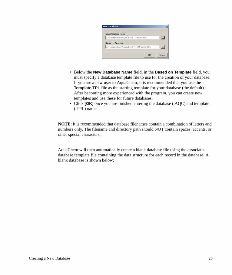
• Below the New Database Name field, in the Based on Template field, you must specify a database template file to use for the creation of your database. If you are a new user to AquaChem, it is recommended that you use the Template.TPL file as the starting template for your database (the default). After becoming more experienced with the program, you can create new templates and use these for future databases.

• Click [OK] once you are finished entering the database (.AQC) and template (.TPL) name.

NOTE: It is recommended that database filenames contain a combination of letters and numbers only. The filename and directory path should NOT contain spaces, accents, or other special characters.

AquaChem will then automatically create a blank database file using the associated database template file containing the data structure for each record in the database. A blank database is shown below:

Creating a New Database 25

At this point you can begin to enter your sample data into the database. You have two options for data entry:

• Data can be entered manually; or • Data can be imported from a text file.

The most convenient option for large data sets is to import the data from a text file; this will be demonstrated below. If you enter your data manually, be sure to first create a minimum of one station, so that you have a pre-existing station to assign to your samples. If the data is imported, the station data can be imported the same time as the sample date or separately.

Before proceeding with the import option, you should ensure that your source file containing your water analysis data is properly formatted. For your convenience, an Excel template is provided with AquaChem, which includes the most common Sample and Station parameters. This file is called Import_Template.XLS and can be found in the root AquaChem installation folder. If you wish, you may use this file for your data set. Simply enter your data, then Save the Excel file under a new name and then import your data to an AquaChem database.

26 Chapter 2: Getting Started

2.1.1 Importing DataTo import sample data into your AquaChem database, please follow these steps:

File from the main menu and then select Import

button beside the File field to locate the source file

ImportData.xls (located in the Program Files\AquaChem directory). If necessary, browse to your AquaChem installation folder to locate this file.

[Open]

to select the import Format for the source file; Samples as Rows or Samples as Columns. For this demonstration, the Samples as Rows mode will be used.

You should now see the ImportData.xls file name in the File field, and a preview of file in the lower half of the dialogue (as shown below):

The remaining import options can be left as is.

[Next>]

In the next dialogue, AquaChem requires you to match the fields in your file to the required AquaChem parameter fields. For the ImportData.xls file, the column headings have already been prepared such that they precisely match up with the required AquaChem field headings. Therefore, there is no need to do manual matching.

Creating a New Database 27

However, if there are blank fields in the AquaChem column, then this indicates that the parameter names in the file are not identical to the AquaChem parameter names, and the fields could not be identified. For example, if your file contained the parameter name ‘Conductivity’, you must match this up to the AquaChem parameter Internal Key ‘Cond’.

If necessary, please refer to the Import section in Chapter 3 for more details on matching parameters during the import.

[Next>]

The next dialogue contains a list of the AquaChem parameters which were not matched up to parameters in the source file. This dialogue allows you to enter constant values for these parameters (optional). For example, if all of the imported samples belong to the same project or the same location and this information is not included in the source data file, you may fill the respective fields during this step of the import. To skip this step, leave these fields blank.

28 Chapter 2: Getting Started

[Next>]

You will then see the following warning prompt:

This option allows you to automatically create one symbol for each unique station in the imported source file. These symbols will be created in the Station symbol group. This is a very helpful feature, which can aid in plotting your sample data later on.

[No] to pass on this feature.

The last dialogue in the import options, contains a summary of the import routine and gives you the opportunity to use the [Save] button to save the import settings. Please check that all of your samples, stations, and parameters have been successfully imported.

[Close]

After successfully importing the data, you will return to the main database window showing your active Samples and Stations. For this data set, there should be 4 stations, with 7 samples taken from each station location, for a total of 28 samples.

2.1.2 Assigning SymbolsThe next step to building a new AquaChem project is to assign symbols to your samples.

Creating a New Database 29

By default, a new database will include two symbol groups: a Default symbol group with just one symbol assigned to each sample, and a Station symbol group, with a unique symbol for each unique station in the database; the station symbols are automatically assigned to the appropriate corresponding samples. You may create new symbol groups, or add symbols to one of the existing symbol groups.

For this demonstration, you will add symbols to the Default group.

Follow the instructions below to create new symbols.

Plots from the main menu and then select Define Symbol or Line

below the Symbol Group, and ensure the Default symbol group is selected.

button and a new field will be added to the list of symbols

type: MW-1 in the new line that is added

<Enter> (on your keyboard) to accept the new name

You will now add three more symbols:

button

type: MW-3 (for the new symbol)

<Enter> on your keyboard

30 Chapter 2: Getting Started

button

type: OW-2 (for the new symbol)

<Enter>

button

type: OW-4 (for the new symbol)

<Enter>

Once you are finished, you should have five symbols listed for the Default symbol group, as seen in the figure below.

Next you need to define the necessary symbol properties:

Symbol #2 (MW-1) from the list

Choose a symbol character from the list of available symbols (in the lower half of the dialogue). Simply click on the desired new symbol shape

Creating a New Database 31

Choose a Color for the new symbol. To access the color options press the button beside Color, and select a color from the list of available

colors

Choose a Size for the symbol; the font sizes are available from the combo box beside Size. (Recommended size is 12pt.)

[Apply] button, once you are finished.

Repeat these steps for the three other new symbols that were created.

Once you are finished creating the symbols and defining the symbol properties,

[Apply]

[Close]

In your active samples list, you are ready to assign these symbols to the samples.

32 Chapter 2: Getting Started

Select the first seven samples in your sample list. To do so, click on the first sample, hold down your left mouse button, and drag your mouse down to the 7th sample.

Samples from the main menu and then select Assign Symbol from the main menu (or use the Assign Symbol icon in the tool bar).

The Assign Symbol dialogue will list the available Symbol group names and the corresponding symbol, as defined earlier.

Symbol 02 MW-1

[Assign]

You will now assign symbols to the next group of samples.

Without closing the Assign Symbol dialogue, activate the Sample list and select the samples from the MW-3 Station- samples 8 to 14. The Assign Symbol dialogue will remain on top; move it if it is blocking the samples.

Click in the Assign Symbol box to make it active.

Symbol 03 MW-3

[Assign]

Repeat these steps to assign symbols to the remaining samples for stations OW-2 and OW-4. Close the Assign Symbol dialogue by clicking the [Close] button when you are done.

Once you are finished, each of your samples should have a corresponding symbol which relates to the location of that sample. In the active list of samples, there is a column heading Symbol which indicates the Symbol group that is assigned to each sample. You should see Symbols 2, 3, 4, and 5 in your sample list, as shown below.

Creating a New Database 33

The samples are now ready to be plotted.

2.2 Creating PlotsAquaChem allows you to plot your sample data numerous different plot types. For this exercise, you will create a simple Piper plot which distinctly shows the four different sample groups. For more details on the AquaChem plots and the plot options, please refer to Chapter 4.

Plots from the main menu, then select New and then Piper

A Piper Plot Options dialogue will appear with default plot settings. The following section describes some of the generic plot options.

To create the plot using the default plot options, click [OK].

The plot should be created similar to the one shown below:

34 Chapter 2: Getting Started

You can modify the plot options by right-clicking on the plot to load the Plot options dialogue.

If you are satisfied with your plot, proceed to the next section titled Printing Plots.

2.2.1 Plot OptionsThere are many common graphical features and options for each plot. When you select any of the graph types to plot (for example Piper plot), a plot options dialogue will appear with default settings for all of the necessary parameters and settings. For most plot types, the Plot Options dialogue contains links to the following dialogues: Parameters, Title, Symbols, Label, Axis, and Legend (not all dialogue options are present on the Piper plot options dialogue. For more information, see Chapter 4)

Creating Plots 35

The main Plot Options dialogue contains information on the parameters/series used in the plot and provides the link buttons to access various dialogues described below, which are used to customize the plot.

• Title Dialogue - contains options for Plot Title font size, Position, and Alignment.

• Symbols Dialogue - contains options for symbols used in the plot, Visibility, Scaled Symbol Size options, etc.

• Legend Dialogue - contains options for displaying a Plot Legend, Legend Title, and display features.

• Labels Dialogue - contains options for data point labeling and positioning.• Axis Dialogue - contains options to customize the axes. • Line Dialogue - contains options to add and customize lines on the plot.

2.2.2 Printing PlotsOnce you have prepared the desired plot(s), you are ready to print.

File from the main menu and select Print, or click the Print icon in the tool bar.

You should then see a Print Options window, as seen below.

36 Chapter 2: Getting Started

The Print Options allow you to choose which plots will be printed, their position, size, and which plot template will be used.

A list of Available Plots will appear in the upper-left corner of this window. This list represents the plots which are currently open in AquaChem. Select the plots you want to print by placing a check mark in the box beside the appropriate plot name.

To select the Piper plot for printing,

Click once in the box beside Piper /1 to activate it and then again to add a check mark to the box. This plot should now appear in the preview window (on the right).

Creating Plots 37

To load additional plots (if you created them in the project), simply click once with your mouse in the box beside the plot name.

The plot will be automatically sized to fit the page layout. If the default page settings are not suitable, you can manually change the position of each plot using the options provided in the Axis tab (Length and Origin).

If you want to display plots on several pages proceed as follows:

• Enter the number of plots per page. • You will be asked to confirm the number of rows and columns on you page.

For example, if you wish to display 8 plots and you enter 2 rows and 2 column, the plots will be distributed on 2 pages.

38 Chapter 2: Getting Started

Next, you can select the page layout by choosing a print template. The print template will allow you to enter information on the page footer such as project information, sample information, and company information.

Under the Page Layout options (on the left side of the window), you will see the default template setting is US-Letter-Portrait.

from the combo box to see all available templates.

You can see a list of plot descriptors in the Page Layout dialogue. They are linked to the fields on the report and you can see the changes made as soon as you leave the field you were typing in:

Next, you will fill in the project specific plot description fields under the Page Layout options. Press the <Enter> key after each entry:

DESCRIPTION: type: Piper plot of samples collected from 1992 to 1998

PROJECT: type: Sample Project

PROJ #: type: 2006-1

Creating Plots 39

CLIENT: type: Client’s name.

DATE: type: Current date

NOTE: The Schlumberger Water Services logo shown in the bottom of the page can be easily replaced with your own company logo. This is done using the Template

Designer option, which can be accessed by clicking the button beside the Template combo box. This option is not explored in this exercise. For more information, please refer to Template Designer section in Chapter 3.

Next, if you have added a legend to your plot, you can add this legend to the printed page, and position it on the page.

Legend tab (below the list of Available Plots, and beside the Axis tab).

Visible (click once in the check box) to activate the legend for the Piper Plot.

The Piper plot legend will appear in the upper-left corner of the page. To move the legend,

X-Axis field and enter a value of 15.

Y-Axis field and enter a value of 25.

If you have loaded the plot successfully, your display should be similar to the one shown below:

40 Chapter 2: Getting Started

[Print] button (in the lower left corner) to send the plot to a printer.

[Close] to close the print options window and return to the AquaChem active samples list.

2.2.3 Exporting Plots as Graphics FileUpon returning to the main AquaChem window, you will see that the active sample list window is open, and you should still have the Piper Plot window open. In addition to printing the Piper plot, you will now save this plot as a graphics file so that it may be inserted into an external report.

Piper plot window to make this the active window

File from the main menu, and then choose Export, and finally, Image.

You will then be prompted to enter a filename for the plot. Browse to the desired folder on your computer, then enter a name for the file. For this demonstration, you will save the file in the AquaChem folder.

Creating Plots 41

type: Piper as the filename for the plot

[Save]

The plot will be saved as a .WMF (Windows MetaFile) graphics file. This file can be opened using most conventional graphics editors, or the file can be directly inserted into a word processor application.

button in the upper-right corner of the Piper Plot window, to close this plot window.

In the next section, the Report options will be briefly demonstrated.

2.3 Creating ReportsAquaChem allows you to choose from 9 data analysis reports and perform 3 different statistical tests on your data. For this demonstration, you will briefly examine the generic Report options and create a Statistics Report. The Summary Statistics report provides a statistical summary of selected parameters for all active samples in your database. For more details on Reports, please refer to Chapter 5.

To create a Summary Statistics report for all samples in the active list:

Reports from the main menu and then choose Statistics, and finally Summary Statistics

A dialogue will load that will allow you to customize your Summary Statistics report. This dialogue contains four tabs: Parameters, Statistics, Options, and Data.

Parameters tabThe first tab that loads will allow you to specify which parameters you wish to use in your Summary Statistics report.

42 Chapter 2: Getting Started

For this example, you will add benzene, Sum of Anions and Sum of Cations to the list of parameters.

button

Select Benzene from the dialogue that loads.

[Select]

Select Calculated Values from the combo box at the top of the dialogue.

Select Sum of Anions from the list.

[Select]

Select Sum of Cations from the list.

[Select]

[Close]

If you wish to add more parameters, you can do so in the manner described above.

To remove a parameter from the list,

Select the parameter to be removed

button

Once all parameters are selected, you can chose what statistics to perform.

Statistics tab.

Parameter Key Unit

Creating Reports 43

Statistics tabThe Statistics tab allows you to select the summary statistics that will be performed on the data for the parameters you selected in the previous tab.

For this example, leave the statistics that are selected by default, however if you wish to add more statistics you can do so in the same manner as adding parameters. Selecting certain statistics will require you to enter additional information. For example, when selecting the Quantile statistic (QUANT), you will need to enter the percentage of the quantile.

When you are finished, move on to the Options tab.

Options tabThis tab allows you to select the output orientation (parameters as rows/statistics as columns or parameters as columns/statistics as rows) as well as providing you with the option to Break by symbol. If this option is selected, the summary report will be generated for every group of samples that bear the same symbol, i.e. every station in this example.

44 Chapter 2: Getting Started

For this example, check the box beside Break by symbol and move on to the Data tab. This will create separate statistics for all samples assigned to the same symbol.

Data tabThe Data tab provides a preview of the data that will be used for the summary statistics report.

The Statistics report window should be shown on your display, similar to the one below.

Creating Reports 45

The minimum, maximum, arithmetic mean, as well as other values of interest will be calculated for the selected database parameters.

Once you are finished, you can Save or Print your report.

2.3.1 Saving ReportsReports can be printed or saved to multiple file formats. The supported file formats are .XLS, .TXT, and .CSV.

NOTE: The pre-defined reports in AquaChem can be saved as .XLS, .TXT, and .CSV. The user-defined reports (e.g. Sample Summary Report created using the Report Designer) can be saved as .HTM or .RTF format.

To save the report,

[Save] button at the bottom of the report window

type: a filename for the report

46 Chapter 2: Getting Started

Select the file type

[Save]

2.3.2 Printing ReportsTo print any of the reports,

[Print] button at the bottom of the Report window; or

File from the main menu and then select Print, while the report window is active.

The Report will then be sent to your default Windows printer, or you may select another printer.

[Close] located at the bottom of the Reports window, to close the window and return to the main AquaChem window.

This concludes the Getting Started chapter.

Creating Reports 47

48 Chapter 2: Getting Started

3AquaChem Menu Commands

This chapter describes each of the items on the AquaChem menu bar. Similar to the AquaChem Toolbar, the menu is context sensitive and main menu items are available only when the active list window is the currently selected window. In addition, menu items will become grey and inactive if there are no available for the current mode.

In this chapter, you will find information on:

• File Menu• Edit Menu• View Menu• Filter Menu• Stations/Samples Menu• Plots Menu• Reports Menu• Tools Menu• Window Menu• Help Menu

Following the menu items, you will find a section on the AquaChem database, which covers the database options that are available for your AquaChem project.

The following sections explain the menu commands in detail.

3.1 File Menu

3.1.1 NewThe New option is only available when no other database is open. In order to activate this option, you must first close any database files which may be open.

The New command creates a new empty database based on a database template. The template is an empty database that contains all necessary data tables, parameters, settings, etc., but does not contain sample or station data. When you create a new

File Menu 49

database, the database template is copied to the specified filename and location. Choosing a database as a template simply means that you will find the same Lookup-tables, Sample/Station Parameters, and Settings in the database as there are in the selected template.

The AquaChem directory contains two default database templates:

• Template.TPL is normally used to create a new database file.

AquaChem lets you save and use any valid AquaChem 5.1 database as a template.

Creating a New Database

Follow the steps below to create a new AquaChem database file:

• Start AquaChem and press [Cancel] when prompted to open a database. (Or if you already have AquaChem opened, close the current open database by selecting File > Close.

• Select New from the File menu, and the New Database dialogue will appear as shown below.

• Browse to the appropriate folder. The default folder is the installation folder Program Files\AquaChem.

• Type in the name of the new database, and click [Save].• You will then see the following New Database dialogue.

50 Chapter 3: AquaChem Menu Commands

• Below the database filename, you must specify a Database Template to use for the creation of your database. By default, AquaChem will use the Template.TPL file which is included with your installation. This template contains the same data structure as the demo database. When you first start using AquaChem, this will be the only database template file available, and in most cases this template file should be adequate. If you have other database templates available, click the button to browse and select a .TPL file to be used for your project.

• Once you are finished entering the .database (.AQC) and template (.TPL) name, press [OK].

NOTE: Database filenames should be a combination of letters and numbers only. The filename and directory path should NOT contain spaces, accents, or other special characters.

AquaChem will then automatically create a blank database file (with .AQC extension) using the associated database template file containing the data structure for each record in the database. An example is shown below:

File Menu 51

If you use the Template.TPL file, then your data structure may contain some parameters which do not apply to your data set, while others, which you might need, may be missing. Use the File > Database options to modify the available parameters in the template. The database options are explained later in this chapter.

3.1.2 OpenThe Open command opens an existing AquaChem database. When you select this command, the following dialogue should appear:

52 Chapter 3: AquaChem Menu Commands

You may open an .AQC file from AquaChem v.4.0 or v.5.0. AquaChem no longer supports direct opening of projects from version 3.7 or earlier. To retrieve data from such a project, it has to be exported to a text, MS Access, or MS Excel file and then imported into a new AquaChem 5.1 database.

NOTE: You may open a database which resides on a network computer. However, only one user should access a database at a time. If you have created you database with an AquaChem version prior to 5.1.20, minor modifications will be applied to your file during opening. You will be informed a backup copy of the original database is created.

After you have selected the desired database, click [Open] to load the file into AquaChem. You may also open a database by picking the file from the recent file list, under the File menu.

The Open database option is only available when no other database is open. In order to activate the Open command, you may need to first select File > Close to close the opened database.

3.1.3 CloseThe File > Close command will close the current database. This will allow you to open other databases, or create a new database.

3.1.4 Save DatabaseSaves the database, or allows you to save the database under a different name and directory. The database file is saved with the extension .AQC.

File Menu 53

3.1.5 Save as TemplateThis option allows you to save the current database settings to a database template (.TPL) file. This new template can be used when creating future databases having the same structure and settings as the currently loaded database.

The Template.TPL file is used only in the initial step to create a database. Similar to a word template which you use to create a new word document, the document is completely independent of the template after the document is created. After the database is created, the Template file is no longer needed. You may add, remove, or change parameters and properties; all properties are stored in the .AQC database itself. If you want that new databases use identical settings as your current database, Do not delete or rename the Template.TPL file, since it is the default database template.

The Save as Template command is only available when a database is open, and the Active List window is active.

3.1.6 ImportThe import option allows you to import Sample and Station data into your AquaChem database. This option is only available when the sample/stations list window is the active window. The Import routine is separated into four simple steps. When you select File > Import from the main menu, the following dialogue will appear:

The source data file must be a text file with the data separated by a tab, semicolon, or comma (extension .TXT, .PRN, or .CSV), an MSExcel file (extension .XLS), or an MSAccess 2000 database table or view. When using a character other than a tab (e.g. a

54 Chapter 3: AquaChem Menu Commands

comma or semicolon), ensure that this character does not exist in any of the text fields in the file. To load the data file, simply press the button beside the File field.

The file format is specified beside the Format field. Use the combo box (as shown below) to select the appropriate file format. The source data file may have the following four formats:

• Samples as Rows - each new row represents a new sample, parameters are listed in columns.

• Samples as Columns - each new column is a new sample, parameters are listed in rows. The only constraint of this format is that one row has to contain the StationID information for the station for which the sample was collected.

• One analyzed value for each Row - each new row contains new measured values. The minimum information that has to be provided in each row is as follows: SampleID (being unique for each Sample), StationID, Parameter name, value, unit (where valid units are: mg/l, ug/l, ng/l). Typically, this format will thus contain further columns with analysis metadata such as MDL (method detection limit), method used for the measurement (Protocol), Precision of measurement, etc. These meta parameters are, however, not required in the import file.

• Station Data only - import just the Station Description fields, such as X, Y, Z, Location, Station Name, Well depth, etc. This can be useful if your source data for stations and measurements is kept in separate files. It is then recommended that you import the station data before analysis results. If you select this option, each station must be in a separate row.

NOTE: Depending on the format, the first row (or column) must contain headers. Optionally, the subsequent rows may contain the unit or the CAS registry number allowing a more accurate matching of the database and import parameters.

The next line in the Import Options dialogue is Settings. This option allows you to use previously defined import settings. This is useful for importing datasets with similar formats. If you do not want to use import settings, then leave the settings field blank. If you want to use previous import settings, press the button to load a list of import configurations:

File Menu 55

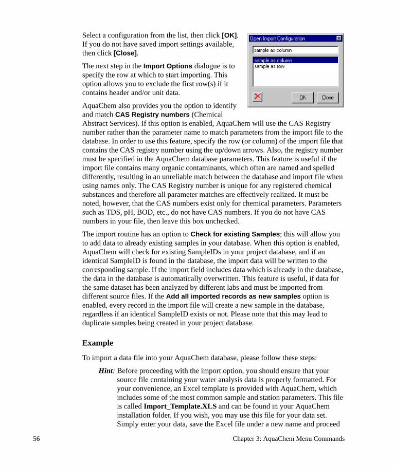
Select a configuration from the list, then click [OK]. If you do not have saved import settings available, then click [Close].

The next step in the Import Options dialogue is to specify the row at which to start importing. This option allows you to exclude the first row(s) if it contains header and/or unit data.

AquaChem also provides you the option to identify and match CAS Registry numbers (Chemical Abstract Services). If this option is enabled, AquaChem will use the CAS Registry number rather than the parameter name to match parameters from the import file to the database. In order to use this feature, specify the row (or column) of the import file that contains the CAS registry number using the up/down arrows. Also, the registry number must be specified in the AquaChem database parameters. This feature is useful if the import file contains many organic contaminants, which often are named and spelled differently, resulting in an unreliable match between the database and import file when using names only. The CAS Registry number is unique for any registered chemical substances and therefore all parameter matches are effectively realized. It must be noted, however, that the CAS numbers exist only for chemical parameters. Parameters such as TDS, pH, BOD, etc., do not have CAS numbers. If you do not have CAS numbers in your file, then leave this box unchecked.

The import routine has an option to Check for existing Samples; this will allow you to add data to already existing samples in your database. When this option is enabled, AquaChem will check for existing SampleIDs in your project database, and if an identical SampleID is found in the database, the import data will be written to the corresponding sample. If the import field includes data which is already in the database, the data in the database is automatically overwritten. This feature is useful, if data for the same dataset has been analyzed by different labs and must be imported from different source files. If the Add all imported records as new samples option is enabled, every record in the import file will create a new sample in the database, regardless if an identical SampleID exists or not. Please note that this may lead to duplicate samples being created in your project database.

Example

To import a data file into your AquaChem database, please follow these steps:

Hint: Before proceeding with the import option, you should ensure that your source file containing your water analysis data is properly formatted. For your convenience, an Excel template is provided with AquaChem, which includes some of the most common sample and station parameters. This file is called Import_Template.XLS and can be found in your AquaChem installation folder. If you wish, you may use this file for your data set. Simply enter your data, save the Excel file under a new name and proceed

56 Chapter 3: AquaChem Menu Commands

with the import options. Or, you may use the ImportData.xls file as a guide; this file is also included in your AquaChem installation folder.

Step 1: Data Source File• Select File > Import from the main menu.• Press the button beside the File field to locate the source file.• Browse to the appropriate folder to locate your text or Excel file then click

[Open]. • Your filename should now appear in the File field, and a preview of the file

should appear in the lower section of the dialogue.• Select the import Format for the source file (Samples as Rows or Samples as

Columns, etc.). For this demonstration, the Samples as Rows mode will be used.

• Select the row from which to start importing.• Enable or Disable the option to Match CAS #’s.• Choose the import option to replace or append the existing samples.

• Once you have entered the necessary details in the first import options dialogue, press the [Next>] button to proceed.

Step 2: Match ParametersThe next step in the Import data options is to Match Parameters.

The Match Parameters frame contains a table listing the Column numbers, the Source text file headers, the Units in the text file, and corresponding AquaChem parameter Internal Key values, as shown in the following Import Options dialogue.

File Menu 57

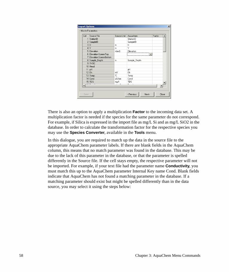
There is also an option to apply a multiplication Factor to the incoming data set. A multiplication factor is needed if the species for the same parameter do not correspond. For example, if Silica is expressed in the import file as mg/L Si and as mg/L SiO2 in the database. In order to calculate the transformation factor for the respective species you may use the Species Converter, available in the Tools menu.

In this dialogue, you are required to match up the data in the source file to the appropriate AquaChem parameter labels. If there are blank fields in the AquaChem column, this means that no match parameter was found in the database. This may be due to the lack of this parameter in the database, or that the parameter is spelled differently in the Source file. If the cell stays empty, the respective parameter will not be imported. For example, if your text file had the parameter name Conductivity, you must match this up to the AquaChem parameter Internal Key name Cond. Blank fields indicate that AquaChem has not found a matching parameter in the database. If a matching parameter should exist but might be spelled differently than in the data source, you may select it using the steps below:

58 Chapter 3: AquaChem Menu Commands

• Double-click in the grid cell under the Aquachem column and a combo box will appear listing all of the available parameters in your AquaChem database.

• Select the appropriate parameter to match to the import Source File column. This will correctly link the parameters in the source file to the parameter names in the AquaChem database template.

• If the parameter to be imported is not included in the database, it may be created prior to importing. Select <create> from the available list. An AquaChem database parameter will be created for every Import parameter that has been mapped to <create> when you click the [Next] button. You will be prompted to enter the required information for each parameter to be created in such way.

• Repeat this step for each parameter in your source file which has not been correctly mapped to an AquaChem database parameter.

Hint: If the field names in the file are identical to the field names in the AquaChem database template file, the parameters will be mapped automatically to the AquaChem column. Therefore, if you format your source file correctly prior to importing, you can save some time in this step.

AquaChem allows you to import concentrations in the units which may be different from the ones specified for this parameter in the database. These values will be converted to the units used in the database during the import. Unless otherwise specified, the units used for that parameter will be identical to those specified in the database parameters options (under File > Database). To change the default units, double-click in the corresponding grid cell under the Units column and you will see a selection of available units (g/L, meq/L, mg/L, mmol/L, mol, ppm, umol/L, ug/L). Select the desired unit, and repeat this for other parameters as needed. The values will be converted into the project units.

File Menu 59

Once you have mapped all units and parameters, press the [Next>] button to proceed.

If you have at least one Import parameter mapped to <create>, the following dialogue will load:

Fill in the appropriate data and click [OK]. Make sure you select the appropriate parameter type using the Type combo box at the top of the dialogue. You may later edit these options later on in File>Database>Parameters. Click [Select] to copy predefined information (CAS number, formula) from a list of predefined parameters. The most important value that needs to be provided is the parameter name. Other values can be specified after the import. If more than one parameter was mapped to <create>, AquaChem will present a new dialogue for each parameter, which was marked with the <Create> flag.

Once the last parameter was created, the dialogue will close and you will move to the next step of the Import routine.

If the data does not appear to be correct, press the [<Previous] button to return to the previous step.

Step 3: Unmapped FieldsThe next dialogue contains a list of the AquaChem parameters which were not matched up to parameters in the source file (ie. Unmapped Fields).

60 Chapter 3: AquaChem Menu Commands

This dialogue allows you to enter constant values. For example, if all of the imported samples belong to the same project or to the same location, but this information is not included in the data, you may fill the respective fields automatically with the specified value during this step of the import. For example, you may read the data from a file called MW-1.xls indicating that all samples were taken from well MW-1. In this case, you would enter "MW-1" as a constant value for location. To skip this step, leave these fields blank.

To proceed to the last step in the import routine, press the [Next>] button. To return to the previous step, press the [<Previous] button.

Upon proceeding, you will then see the following prompt:

This option allows you to automatically create one symbol for each unique station in the Station symbol group and assigns this symbol to the appropriate samples.

[Yes] to accept this feature, or [No] to ignore this option.

File Menu 61

Step 4: Result ScreenThe last dialogue in the Import options is a summary of the results of the data import.

The Result Screen dialogue shows the Number of new Samples and Stations that were successfully imported, and the Number of parameters that were successfully mapped and imported.

Before closing the import routine you can save your import settings by clicking the [Save] button. This option allows you to save the import settings (file format, mapped parameters, units, factors, and constant values) for future use. When you click the [Save] button you will be prompted with a Save Import Configuration dialogue as shown on the right hand side. Simply enter a name for the import configuration, click [OK] and then [Close]. After successfully importing the data, you will return to the main database window showing your active samples and stations. This concludes the necessary steps for importing data.

Once you are finished, press the [Close] button.

3.1.7 ExportThe Export option allows you to export the data or plots for use in other applications such as Visual MODFLOW and HydroGeo Analyst. The Export command is only available when the Active List window or a graph window is currently active.

62 Chapter 3: AquaChem Menu Commands

ImageWhen any graph window is active, the File>Export>Image option is available. Clicking this option will load the following dialogue:

You have the option of saving the image in .WMF (Windows metafile) format.

ESRI ShapefileThis option is available only when you have the Active Samples list or a Map plot active and it allows you to export the data as an ESRI shape file (.SHP).

If the Active Samples list active, selecting this option will load the following dialogue:

Use the button to add parameters to export (X and Y coordinates are selected by default and cannot be removed).

File Menu 63

To create the destination file, click the button beside Filename field. The following dialogue will load:

Type in the name of the destination file that you wish to create and click [Save]. You will be returned to the previous dialogue and the File name field will now be filled with the appropriate address.

Click [Export] to export this point theme shapefile. The values for all specified parameters will be included for every point in the attribute table.

If a Map plot is active, selecting the File>Export>ESRI Shapefile option will produce a point or a polygon theme shapefile depending on the currently active symbol type. If the map shows a plain symbol, scaled symbol or a pie plot, then a point theme will be created holding all the chemistry per point in the attribute table. For example, for a pie plot - all parameters; for a plain symbol - just StationID. If the map plot shows a Stiff or Radial diagram per sampling point, then the respective diagrams are exported as polygons, along with the current symbol label, and the data attributes. Since these polygons are defined in map coordinates, you should optimize the symbol size in AquaChem according to the final map scale in HydroGeo Analyst or ArcView.

Type in the name of the destination file and click [Save] to export the file.

DataThis menu item is available when the Active Samples list or a plot is active.

To export your sample/station data, select File>Export>Data while the Active Samples list is active. The following dialogue will load:

64 Chapter 3: AquaChem Menu Commands

Data may be exported in 2 formats: Samples as rows and One row per value. The One row per value format means that for each parameter the stationid, sampleid, value, unit, analysis comments, precision, MDL will be exported. This allows you to export the complete information into an export file. However this format is less convenient if data is to be used for plotting, statistics, etc. In the case of the standard One row per sample format, only the concentration value for each measurement result will be written to the export file.

• By default, all the parameters are selected and will be exported.• To remove parameters from the export, highlight the parameter you wish to

remove and click the button. • To add parameters to the list, click the button and select from the

parameters list that loads. • You may choose the parameter names or the parameter labels to be used as

headers in the destination file. Parameter labels are a good choice if you wish to create a table or a presentation. Parameter names should be considered if the exported table should be re imported back into a different AquaChem database, as the parameter names will match automatically.

• Click the button beside the File name field to create the destination file. The destination file can be of type .PRN, .TXT, .CSV, and .XLS.

• Click [Save] to generate the file.• Once you are finished, press the [Export] button.

You may also export data that was used to generate a specific plot. This feature is useful if you wish to use this data in another plotting program. To export plot data, select the plot you wish to export the data for and then select File>Export>Data. Once a window containing the pertinent data loads, you have a choice of printing the data or saving it as a .TXT, .CSV, or a .XLS file.

File Menu 65

Visual MODFLOWThe Export > Visual MODFLOW option will export your current sample and station data to a space-delimited text file. The data can then be used for the input (concentration observation well data) of a Visual MODFLOW groundwater model.

To export the data:

• Select File>Export>Visual MODFLOW from the main menu.• Click the button beside To File to generate the destination file. This file can

be a .TXT, .CSV, or .XLS file.• Select the Type of data to export. The default is Single Station/Parameter,

however you may choose Multiple Stations/Concentrations as well. See below for a more extensive description of the second option.

• Select the Start Date• Select the Target Time Unit• Select the Station to export• Select the parameter to export• Click [Export] to export the file

Each line in the generated file will have a time measurement and an observed concentration for a single parameter. The start date is used to calculate the time for the first observation.

NOTE: The [Export] button will become active only after the necessary options have been specified.

• If you choose Multiple Stations / Concentrations format, then the dialogue shown below will appear:

66 Chapter 3: AquaChem Menu Commands

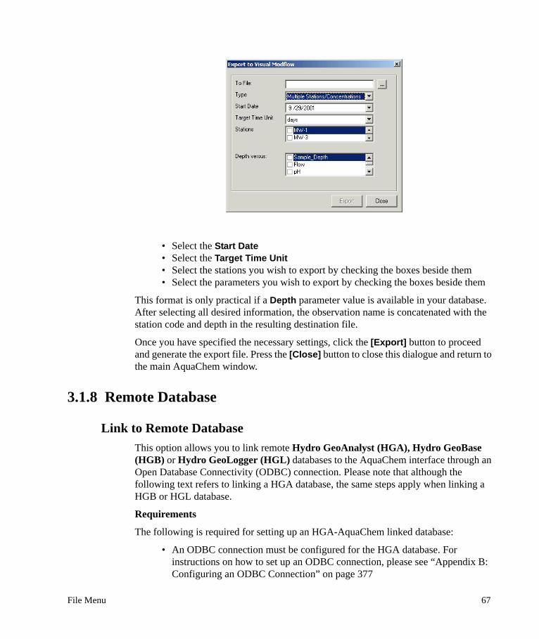
• Select the Start Date• Select the Target Time Unit• Select the stations you wish to export by checking the boxes beside them• Select the parameters you wish to export by checking the boxes beside them

This format is only practical if a Depth parameter value is available in your database. After selecting all desired information, the observation name is concatenated with the station code and depth in the resulting destination file.

Once you have specified the necessary settings, click the [Export] button to proceed and generate the export file. Press the [Close] button to close this dialogue and return to the main AquaChem window.

3.1.8 Remote Database

Link to Remote DatabaseThis option allows you to link remote Hydro GeoAnalyst (HGA), Hydro GeoBase (HGB) or Hydro GeoLogger (HGL) databases to the AquaChem interface through an Open Database Connectivity (ODBC) connection. Please note that although the following text refers to linking a HGA database, the same steps apply when linking a HGB or HGL database.

Requirements

The following is required for setting up an HGA-AquaChem linked database:

• An ODBC connection must be configured for the HGA database. For instructions on how to set up an ODBC connection, please see “Appendix B: Configuring an ODBC Connection” on page 377

File Menu 67

• Please ensure that the HGA database does not contain duplicate parameter names in the following tables: station, sample and result. Aquachem requires the parameter name to be unique for all field names in these tables, whereas in HGA, only fields within the same table must be unique. Typical duplicates are Names, used in the result table and station table, or TOC as top of casing in station table and total organic carbon in the chemical parameters. Please delete or rename duplicate fields before proceeding. NOTE: If you are using the SWS Environmental database template provided with HGA, HGB & HGL, please ignore this requirement.

Follow the steps below to link your HGA database to the AquaChem interface.

[1] Launch AquaChem [2] Create a new empty AquaChem database. Please see “New” on page 49 for

more information on creating a new empty database. It is important that a new AquaChem database is created as once the tables are linked, the AquaChem tables are deleted and data may be lost.

[3] From the main menu, select File \ Remote Database \ Link to Remote Data-base. The following dialog will display:

From the ODBC Data Source combobox, select the ODBC configuration that will be used to link tables from the remote database. If your HGA database does not appear in the combobox, review the ODBC connection settings to ensure it is set up correctly.

Once the database is selected, its corresponding server information will be shown in the Server and Database field.

There are two modes in which you can link your external database: Express and Customized. The express mode provides an automated linking process for HGA databases that were created using the SWS Environmental database template (version 4 only).

68 Chapter 3: AquaChem Menu Commands

For advanced users with customized HGA database structures, the Customized mode allows you to manually link the appropriate chemistry tables, fields and parameters. The following sections describe each mode in more detail.

If you are using the customized linking process, please skip to “Customized” on page 70 for the remaining steps.

Express (HGA Environmental Template v.4.0 only)The express mode will automatically link the following Environmental database tables: Station, Parameter Result and Parameter Sample. To proceed with the linking process, follow the steps below.

[4] Click the [Next] button to begin the automated linking process. The following warning message will show:

Before proceeding it is highly recommended that you back up your HGA database.

[5] Click the [Yes] button to continue.[6] If the linking is successful, the following message will show:

[7] Click the [Ok] button[8] Close the Link Tables dialog by clicking the [Close] button[9] From the main menu, select File / Close to close the current AquaChem project[10] From the main menu, select File / Open to reopen the AquaChem project.

Locate the project file in the Open Database dialog and then click [Open][11] Upon reopening the project, you may receive the following message:

Before continuing, AquaChem needs to initialize some fields in the HGA database. Select the [Ok] button to continue.

File Menu 69

[12] In some cases the following message may appear:

This message will show when there are duplicate field names in the station table and the sample table. If your HGA database already contains chemistry data, it is likely that this message will show. Simply click [Yes] and AquaChem will fix the problem.

Now that the tables have been successfully linked, any changes made in one application, will show in the other. For example, if you modify a station name in the AquaChem station table, this change will also show in the HGA station list, and vice versa.

Please note that AquaChem is now accessing data from a SQL Server database. This means that the SQL Server must be running and you must be connected to the server in order to access its data.

Customizedcontinued from “Link to Remote Database” on page 67

Customized HGA databases, i.e., databases that have been designed and/or modified through HGA’s template manager , can be linked manually to AquaChem using the customized linking mode.

Please note that this mode requires an in-depth knowledge of your HGA database structure and the AquaChem data model, and should be reserved for expert users only. It is highly recommended that you back up your current HGA database before proceeding. Because this process can potentially be complex , SWS offers converting customized databases to HGA linked format as a service. For more information on this service, please contact SWS directly.

[4] Click the [Next] button to continue with the customized linking process. The following dialog will display:

70 Chapter 3: AquaChem Menu Commands

For D_Station, D_Sample and D_Analysis (main chemistry tables used by AquaChem) select the corresponding HGA tables from the comboboxes. You can access the comboboxes for all fields in all dialogs by clicking on the far right end of the field (indicated in the image above) Note: Your chemistry table names may be different than the ones that appear in the shown screen captures. The other listed tables (M_Parameter, M_Guideline, etc) do not usually exist in the HGA data model yet and need to be created. Therefore leave the entries for these tables as <create>.

Once the tables have been defined, click the [Next] button. The missing tables and fields are now created in the HGA data model.

[5] The next step requires that you define the relations between the tables that were defined and/or created in the previous step.

File Menu 71

In the dialog shown above, the table names are listed in the left grid. When a table name is selected, its corresponding required fields are listed in the adjacent grid. For each required field, select the appropriate HGA source field from the field’s combobox. The local fields for each table are described below:

In most cases the default values can be accepted. If one of these fields is blank, this means that the default value does not exist in the respective table and you have to select a field from the list of fields, for this table.

Once the table relations have been defined, click the [Next] button to proceed to the next step.

AquaChem will now create the missing tables and initialize the parameter table. For databases with many rows in the result table, this can take awhile.

[6] In this step, the local AquaChem tables will be deleted and replaced by linked HGA tables. If your current AquaChem table contains data, it will be lost

Table Field Description

Station Station_PK Primary key for station table

Parameter Sample Sample_PK Primary key for sample table

Sample_Station FK Station foreign key

Sample_Samplecode Unique identifier for sam-ples

Parameter_Result Result_PAR_ID Numeric parameter foreign key in result table used by AquaChem, i.e., PAR_ID

Result_Sample_FK Foreign key to sample table

Result_Sample_Qualifier

Column holding the “<“ description code

Result Value Column holding the param-eter concentration value

Result_Sample_Code Alphanumeric foreign key to sample table used by HGA, e.g., Sample_ID

Result_Parname Column holding the chemi-cal name

72 Chapter 3: AquaChem Menu Commands

during this step. This is why you should start with an empty (new) AquaChem project. In the dialog shown below, click the [Next] button to continue.

[7] The next step requires that you map the station table parameters to the station parameters used in AquaChem. In the dialog shown below, you must map all parameters marked in yellow. If a mandatory parameter does not exists, simply select <Create> from the list box. AquaChem will then create the parameter on the fly and assign it to the AquaChem parameter.

Once the station table parameters have been mapped, click the [Next] button to continue.

This mapping process is also required for the sample and measured parameters, as well as the fields describing every measured value, i.e., comment, precision, method, detection limit etc. This mapping is done in the remaining steps.

File Menu 73

[8] This step requires that you map the sample parameter fields. As in the previous step, you must match all fields highlighted in yellow, or set to <create> if the field does not exist..

Click the [Next] button once the mandatory fields have been mapped.

[9] Next, map the measured parameters, such as calcium or chloride. Once mapped, click [Next] to continue.

[10] Finally, map fields that are used to describe the measured results such as precision, filtered/unfiltered, protocol etc. Remember, if these fields do not

74 Chapter 3: AquaChem Menu Commands

exist in your HGA data model, select <create> and AquaChem will create these fields. Click the [Next] button to continue.

[11] AquaChem will now prompt for input for every parameter that was specified to <create> in the previous steps. For chemical names, it will try to detect the parameter from the master chemical table and provide the default values for formula, formula weight, valance etc (shown in the dialog below). If AquaChem cannot find the parameter in the chemicals table, you may confirm the default settings (Name, Form Label and Description), leave the remaining fields black, and alter the parameters later using the File / Database menu.

When prompted with the Create Field dialog (shown above) click the [Ok] button to confirm/accept the field values.

[12] After creating these parameters AquaChem checks if all parameter names are unique. Remember, AquaChem requires unique parameter names across the station, sample and results table. If duplicated names are found, a message such as the one below will be shown. Duplicate names must be removed within HGA by either renaming or deleting these fields. Typical examples of duplicate

File Menu 75

fields include: “Name” (found in station and result table), “TOC” (station top of casing and chemical parameter Total Organic Carbon).

Click [Ok] and eliminate the duplicate parameters in your remote database by either renaming or deleting the mentioned fields.

[13] Once the linking process is complete, the following message will be shown:

Click the [Ok] button, then click the [Close] button and then reopen your AquaChem project,

[14] Upon reopening the AquaChem project, you may be prompted with the following message:

This message is likely to appear if you have previously imported data into HGA using the DTS tool. Simply press [Ok] button and AquaChem will complete the field initialization.

Now that the tables have been successfully linked, any changes made in one application, will show in the other. For example, if you modify a station name in the AquaChem station table, this change will also show in the HGA station list, and vice versa.

Please note that AquaChem is now accessing data from a SQL Server database. This means that the SQL Server must be running and you must be connected to the server in order to access its data.

Note: After linking, some of the linked fields, e.g., sample_id, may not show as visible in the station and sample tables in AquaChem. To make them visible, go to View \ Options and add the fields in the sample/station list options.

76 Chapter 3: AquaChem Menu Commands

Import Linked TablesIf you are connected to a HGA linked SQL Server database, you can use this option to covert the linked tables to a MS Access database format (*.aqc). This allows you to use the database without a connection to the SQL Sever.

When this option is selected, the following message will be shown:

Click the [Yes] button to proceed.

A save dialog will display prompting you to specify a name and location for the database. Once specified, click the [Save] button.

When the tables have been converted to MS Access database format, the following message will be shown.

3.0.1 Print The Print command will load the print options for the current AquaChem window or dialogue. The print icon in the toolbar serves the same purpose. The Print option is only available when one of the following windows is active:

• Plots • Tables (Spreadsheet View), or • Reports

Please refer to Chapter 4: Printing and Exporting Plots for more details.

3.0.2 Template DesignerUse the Template Designer to customize the pre-defined printing templates shipped with the AquaChem demo database, or to create new ones.

File Menu 77

Template Designer InterfaceWhen you select Template Designer from the File menu, the following window will appear:

The Template Designer dialogue has three main components:

[1] Available Templates in the upper-left corner containing the Template Name and a combo box listing the available templates.

[2] Template Details is located immediately below the Template Name field. This includes the controls and tools for designing templates, such as:

• Lines, • Fields, • Labels• Graphics, and •Margins

[3] Preview Window on the right side of the dialogue, containing a preview of the Template as content is added or modified.

The options in the Template Designer allow you to:

• Select the page size, orientation, and margins

Available Templates

Template Details

Preview Window

Pageguide

78 Chapter 3: AquaChem Menu Commands

• Draw lines and borders• Define and position text block descriptors• Position user-entry fields• Add headers and footers, and • Position and size bitmap graphics for a company logo• Adjust the margins of the plot display area

The following section provides more details on the functionality of the template designer.

Template Designer ControlsThe main controls and tools for the Template Designer are on the left side of the main dialogue (as shown in the figure below).

At the top of this frame, you will see a list of the available templates; you can select a different template from the combo box. AquaChem includes the following pre-defined templates:

• US Letter - Portrait• US Letter - Landscape• A4 - Portrait• A4 - Landscape

In the Template Designer dialogue:

• Click button to add a new item to the template.

• Click button to delete the currently highlighted item.

Note that the buttons are common to each tab. For example, if you are in the Lines tab and you press the button, a new border line will be added. You can then proceed to enter the appropriate properties for this line in the fields below.

The button in the Template Designer dialogue will load a Template Name dialogue as shown on the right. It displays the full list of templates currently available and will allow you to create and name new templates.

In the Template Name dialogue:

• Click button to create a new template• Click button to remove an existing template

To rename a template simply place your mouse cursor in the appropriate field, then enter a new text label. Once you are finished in this dialogue press [OK].

File Menu 79

When positioning a line, field, or graphics, the X, Y page coordinates displayed in the lower left section of the main Template Designer dialogue can be helpful. These coordinates correspond to your mouse cursor location and can help you in the placement of the start and end points.

The [Duplicate] button will duplicate the currently selected template. The duplicate template will be named Copy of TemplateName, and the duplicate template will have the same layout and characteristics as the originally selected template. If it is your first time creating or customizing a Print Template, it may be easier to modify a duplicate copy of an existing template, than to start from the beginning. Please note that each Template must have a unique name.

NOTE: Although you have the option of modifying the default template designs, it is strongly advised that you either duplicate the selected template, or create a new blank template. This avoids damaging or losing the original template designs and ensures you will always have a standard set of default Print Templates.

When you press the [Page Setup] button, the following Page Setup dialogue will appear:

In this dialogue, in the upper Paper section you can define paper Size and Source.

In the lower Orientation section, you can define paper orientation and page Margins for the template. The page margins will correspond to the location of the page border. The page dimensions inside the margins will be used to automatically locate and size the selected plots.

80 Chapter 3: AquaChem Menu Commands

You can also access your standard Windows Printer options by pressing Printer button. Once you are finished, press [OK] to return to the previous dialogue.

Creating New Templates - ExampleThe following section describes the options of the Template Designer, and how it can be used to build and customize your own templates. The brief instructions below tell you how to create a basic printing template, and how to customize this to your own preferences.

• Click button to load the list of Templates.• Click button to create a new template.• Enter a name for the new template (e.g. “Sample-Letter” for these instructions).• Press [Close].• Choose this template from the combo box.

You will then see a new blank Print Template in the preview window. By default, all new templates include a border and default page settings.

Creating Lines

The first tab in the template designer dialogue is Lines. This tab allows you to create the Print Template form by drawing lines indicating the borders of the template Title Blocks. Each line has a Name, Width, starting coordinates (X1, Y1), and ending coordinates (X2, Y2). The coordinates units are in cm. The coordinates are measured from the origin, which is the bottom left corner of the page.

In the Border frame you can show/hide the page border using the check-box, as well as set the border width.

To create a new Line:

• Click button and a new Line will be created with the name new Line#.

• Double-click in the Name field and enter a unique name for the new line (e.g. Line2).

• Enter a line Width 0.2.• Enter the desired start and end

coordinates for the new line (X1, Y1 represents the starting point of the line, and X2, Y2 represents the end point of the line). The bottom-left corner of the Preview Window serves as the origin for the Template designer.

To edit an existing line, select the line from the list and enter the new coordinates. For example, if you want to start a line at a point located

File Menu 81

1.5 cm from the bottom of the page and 1.5 cm from the left side of the page, you would enter a line with X1 = 1.5 and Y1= 1.5 (cm). Remember that you can always use the mouse pointer to check the page coordinates, as shown on the left side of this dialogue.

If you want to enter line locations to coincide with margin locations, enter the following items for the X or Y coordinate:

Enter “L” to have a line coordinate equal to the left margin location.

Enter “R” to have a line coordinate equal to the right margin location.

Enter “T” to have a line coordinate equal to the top margin location.

Enter “B” to have a line coordinate equal to the bottom margin location.

This is useful if you want the lines to automatically adjust as the page margins change. An example is shown below:

In this example, a line would be located at a height of 4 cm from the bottom of the page (Y1 and Y2 = 4) and the line would extend from the left page margin (X1 = L) to the right page margin (X2 = R) as shown below.

NOTE: To allow for quick recognition, the selected line, field or label is colored in red in the preview window. This will help you to quickly choose the starting and end points.

82 Chapter 3: AquaChem Menu Commands

To remove existing lines, select the line then press the button. The template designer settings will automatically be saved to the database; as such there is no [Save] button required in this dialogue.

Creating Fields

The next two tabs in the template designer are Fields and Labels. These provide options for adding text to the template. The fields tab is used to create, position and label the Text fields. Beside each field, there will be a corresponding label.

The Text fields are the items which will show up when you load the template into the print preview window. They will be blank and prompt you to enter the specific details.

To create a new Field:

• Click button and a new Field will be created with the name new Field#.

• Enter a unique name for the field.• Enter the appropriate page coordinates

for the field (the position refers to the page coordinate location for the bottom-left corner of the field). Remember to leave room for the Label which will typically be placed to the LEFT of the field.

• Select an appropriate font for the field. Click once in this field, and you should see a button will appear. Press this button to access the font options for this field.

To modify an existing field, select this item from the combo box, and make the desired changes to the position, text value and/or font. The button can be used to remove existing fields from the template.

The next step is to create a Label for the Text Field. As mentioned above, the Label is commonly positioned immediately to the left of the Field, using the same Y-coordinates. Therefore, take note of the Y-coordinates for the field(s) you just created, so they can be used for the corresponding label.

Creating Labels

The fixed text Labels are hardcoded into the template; this means that this item will always show up once the template has been selected, and will be Read-Only in the print options window. Beside each label, there is a Field entry, which receives the actual text entry for the printout when the template is loaded (information is entered into the fields in the print preview window).

File Menu 83

For example, a label item would be Date; beside the date, there would be a Date field. When the template is loaded into the print options window, you will be prompted to enter a date in the Date field, which corresponds to the plot or report(s) which has been selected for printing.

AquaChem allows you to specify multiple labels at any location on the page. These labels generally contain static project information such as Client, Project number, and Date.

The Labels tab allows you to create, position and customize the Labels on the template.

At the top of this dialogue, there are defaults for a Header and Footer for the template. The header position (Left, Center, or Right) can be adjusted along with the font (press the button to access the font options for the Header or Footer). If you do not want a header or footer, simply leave this field blank.

In the lines below, you will see the list of labels.

To create a new label:

• Click button and a new Label will be created with the name new Text#.

• Enter a unique name for the label. • Enter the appropriate page coordinates

for the label. (X1, Y1 refers to the page position for the bottom-left corner of the label). It is common to position the label to the left of the corresponding field. If necessary, use the preview window as a guide.

• Select an appropriate font for the label. Click once in this field, and you should see a button appear. Press this button to access the font options for this label.

To modify an existing Label, select the item from the combo box, and make the desired changes to the position, text value and/or font. The button can be used to remove existing Labels from the template.

Creating Graphics

The Graphics tab in the template designer dialogue allows you to import graphics (.BMP, .GIF, or .JPG) into the template design.

84 Chapter 3: AquaChem Menu Commands

You may set the position of the image on the page and specify the size as it will appear on the page. Each of the default Print Templates has been designed to accommodate an imported bitmap image of your company logo or your client’s logo (or any image). AquaChem supports common graphics files .BMP, .GIF, and .JPG.

To import a new bitmap image file:

• Click button and a new Graphics entry will be created with the name new Picture#.

• Enter a Name for the new graphics.• Click once in the File field and a

button should appear. Click this button to browse the bitmap image file (filename.BMP) and then to import the image click [Open].

• Enter the position coordinates of the bitmap (the position of the bitmap refers to the X-Y page coordinates for the top-left corner of the bitmap image).

• Enter the Width and Height of the selected bitmap file. The dimensions of the bitmap image refers to the Width and Height of the bitmap image as it will appear on the page. The bitmap image will be automatically re-sized (e.g. stretched or compressed) to fit the dimensions.

• You may also use the navigation and reduce/enlarge buttons to change the position and size of the label.

To modify an existing bitmap file, select the graphics from the combo box, and make the desired changes to the position, name, or dimensions. The button can be used to remove existing bitmap logos from the list.

File Menu 85

Adjusting Plot area MarginsThe Margins tab in the template designer dialogue allows you to define the area that may be used for placing plots automatically. For example, if the template includes figure information at the bottom of the page, setting a margin of 5 or 6 cm will prevent the automatic plot placement from using this area and the plots will not overlap with these template elements. This is done by simply entering the distance (cm) form each side of the page you would like the display area to be confined to in the appropriate field (Top, Bottom, Left, and Right).

You can also turn the page border on or off using the Show check box and set the width of the page border line by entering an appropriate value (mm) in the Width field.

This concludes the steps for creating Print Templates.

3.0.3 PreferencesThe Preferences dialogue loads the general user preferences for AquaChem. These can be accessed only when the sample/station list is active. This dialogue contains four main tabs: General, Plots, PHREEQC, and Censored Data as shown below. A detailed description for each of these tabs is provided in the following section.

86 Chapter 3: AquaChem Menu Commands

General

Interface Colors frame

In the Interface Colors dialogue, you can specify the AquaChem MDI (Multiple Document Interface) main program window Background color. Simply click on the

button and a standard windows Color options dialogue will load allowing you to choose another color.

Water Quality Standards frame

In this frame, you can specify the set of Water Quality Standards to be used for the current database in AquaChem. Multiple standards and levels can be set to active, allowing you to check values against a mix of levels, e.g. ODWS and PWQO, or USEPA and WHO. Values exceeding the respective water quality standards will be highlighted using a color code when displaying the data. You may change the color that should be associated with every level of exceedence by double-clicking on the color for respective level.

The data for each Water Quality Standard is specified in the Database dialogue which can be accessed through File > Database > Water Quality Standards. There, you may edit existing values for the standards for each parameter. You can also create your own set of Water Quality Standards and import or manually enter values for these new standards.

Viewing Guidelines

Guideline exceedences can be viewed in the sample details table. However, when multiple guidelines are active, there is no legend to find out what exceedances a highlighted cell indicates.

File Menu 87

To view all the guideline exceedences for a parameter in the sample details table, simply click on the highlighted cell, and then right-click to display the Parameter Details dialog (shown below).

All the active guidelines that are exceeded are displayed at the bottom of the dialog, as indicated in the image above.

Seasons frame

Use the Project Location combo box to select the hemisphere for your project site. Depending on the hemisphere, the seasons may be reversed. The seasons are counted beginning with Spring (March 21 to June 20), in the Northern Hemisphere and Fall in the Southern Hemisphere.

To view which season returns which number, consult the Calculations tab of the Database.

Document root frame

Use the Document Root field to specify the path to the folder, containing documents that are referenced from AquaChem records. Sample or station text fields may contain filenames or internet addresses. For filenames, you may indicate the full filename including the path or only the filename. In latter case, this file must be reside in the documents root folder. This is convenient, if the documents have to be moved to a different location. Since all reference files reside in the root folder, only the document_root parameter has to be changed to indicate the new location. If the files are specified including the full file path, then all records referencing the moved files must be updated.

PlotsThe second tab in the Preferences dialogue contains settings for Plots which is used for the settings in the Plots and Symbols.

88 Chapter 3: AquaChem Menu Commands

Active Plots

The upper left frame of this dialogue lists the Active Plots. This allows you to activate / deactivate the plots. Deactivated plots will not appear in the Plots menu (main toolbar). This allows you to hide plots which are never used from the menu. Active Plots are indicated by the presence of a checkmark beside the plot. By default, all plots are active.

Symbol Font

In the upper right frame of this dialogue you will see options for the Symbol Font. AquaChem now uses “True type fonts” for symbols on plots and graphs. As such, there is an unlimited number of symbols that you can use for your project database. The default font selection is WHI_Symbol. To choose another font type, press the button.

NOTE: The symbols can be defined for samples through the Plots > Define Symbol or Line dialogue.

Plot Title Options

This frame includes settings for the automatic plot titling option. When a new Pie, Radial, or Stiff plot is created with your samples, the plots will automatically be titled with the descriptive fields (parameters) listed here. You can specify which parameters you would like to be utilized when using the automatic title option.

To do so, click the or button to add or remove parameters. To change existing fields, simply double click in the field and choose a new parameter from the combo box. The parameter order can be arranged using the up and down buttons. Once you are satisfied with the parameters, you must

File Menu 89

specify a Field Separator. This will be the character that separates the parameters in the title of the plot. You can use any character as the field separator, however the most common are a space, hyphen, comma, or a semi-colon.

Based on these preferences, all new Pie, Radial and Stiff plots will be titled with the unique descriptive parameters for the individual sample. Using these parameters above, you can see an example of a Pie Plot which is created with the automatic title option.

The title of the Pie plot uses Sample_Date (8/15/1992), SampleID (MW-1-92), and Location (Waterloo), separated by a comma.

The Plots tab also allows you to choose in which color the selected samples are highlighted when a symbol is clicked. For example, if you use red often as symbol color, you may want to select a different highlight color in order to distinguish which symbols are selected and which ones are not.

PHREEQCThe third tab in the preferences dialogue has options for PHREEQC; this controls specification of PHREEQC related Files and Folders.

90 Chapter 3: AquaChem Menu Commands

Files and Folders

In this dialogue (shown below), you must specify the locations of the PHREEQC Thermodynamic Database (phreeqc.dat) and the PHREEQC Executable (phreeqc.exe) files. These files are required for running PHREEQC simulations.

Under the Files and Folders frame, press button beside the Thermodynamic Database field and select the path and filename from the PHREEQC Thermodynamic Database dialogue. From this dialogue, select either phreeqc.dat, Wateq4f.dat, Pitzer.dat, or Minteq.dat. In addition, in the PHREEQC Executable field select the path and filename for the phreeqc.exe file. Finally, specify the path and filename for the USGS graphic user interface (PHREEQCI or PHREEQC for Windows executable, if this component is installed). To change the directories for these files, press the button beside each directory path, and specify the new file/folder location.By default, all PHREEQC input and output files will be saved in your AquaChem installation folder (default is Program Files\AquaChem).PHREEQC-I or PHREEQC for Windows is required for Advanced PHREEQC Simulations.

Once you are finished, click [Save] then [Close]. You are now ready to run PHREEQC.

Non-detectsData generated from chemical analysis may fall below the method detection limit (MDL) of the analytical procedure. These measurements are generally described as nondetects, (rather than as zero or not present) and the appropriate limit of detection is usually reported. In cases where measurement data are described as not detected, the concentration of the chemical is unknown although it lies somewhere between zero and detection limit. Data that includes both detected and non-detected results are called censored data in the statistical literature. (Office of Environmental Information, U.S. Environmental Protection Agency, 2000).

File Menu 91

In AquaChem database the non detects are entered with a “<“ sign. This tab allows you to specify settings for handling censored data in plots and calculation.

Concentrations which are greater than the upper concentration limit the analysis method can handle are rare in modern databases, since remeasuring the diluted sample normally solves the issue. However such “greater than” concentrations can occur in historic data sets.

In this dialogue, you are presented with options for displaying non detects in plots and all calculations except the Summary Statistics as mentioned above. AquaChem allows you to enter and store approximate measured values using the less than (<) and greater than (>) symbols. These options require you to specify whether these approximate values will be ignored or included in the plots.

• If you choose to Ignore non detects with graphics or calculations, they will be treated as null entries.

• If you choose Don’t ignore non detect results, you may specify by which factors <> these values are multiplied for the use in plots or calculations. For example, if 2.0 and 0.5 are specified, a value of >10 will be taken as 20, and a value of <10 will be taken as 5.

3.0.4 DatabaseThe File > Database command loads the AquaChem database options for your current database. This option is only available when the active list is the current window. For details on the Database options dialogue, please refer to The AquaChem Database section at the end of this chapter.

3.0.5 ExitThe Exit command will exit AquaChem. Ensure that all changes are saved to your database before exiting the program.

3.1 Edit MenuThe Edit menu provides access to commonly used Windows tools such as Cut, Copy, and Paste. The Cut, Copy, and Paste commands are not available when the active list

92 Chapter 3: AquaChem Menu Commands

window is the active window; these options are only available when you are viewing or editing data for a sample or a station.

3.1.1 CutCuts selected data from the field and places it on the Windows Clipboard.

3.1.2 CopyCopies the selected data or plot to the Windows Clipboard.

3.1.3 Paste Pastes data from the Windows clipboard into the selected field. In order to paste numerical values into a sample details field, the field must be active, which is indicated by a flashing cursor in the field. Simply double-click in the appropriate field to activate it and it will be ready to accept data from the clipboard.

3.1.4 ReplaceThe Replace command allows you to replace data for an individual parameter with a new value for all active samples in the database or to multiply all existing values by a specified factor.

Simply choose the method you wish to apply and the parameter you wish to apply this change to from the combo box beside Parameter. Then enter the value to replace or multiply by in the field beside the method combo box. Once you are finished, click [Apply]. A warning message similar to the one shown below will appear:

Choose [Yes] to proceed or [No] to cancel the operation.

The Multiply by method may be useful for correcting import errors. E.g. the X coordinates can be multiplied by 1000 in order to convert the inadvertently imported

Edit Menu 93

km values into meters. Note that this method can also be used to bulk edit analysis meta information such as Protocol or Method Detection Limit. For example if you know that in all imported samples, the detection limit of mercury is 1 ng and the method 245.1 was used for analysis, the replace feature is the fastest way for updating this information. Alternatively this information has to be entered manually in the sample detail screen, if it was not included in the import data source.

3.1.5 FindThe Find dialogue allows you to create SQL-like queries of the samples or stations in the AquaChem database.

You may run a Simple, Result meta data, or Complex search. A simple search allows you to specify one criterion based on Station, Sample, or Measured values. A meta data search allows you to search for result meta data, e.g. all samples where the method detection limit of mercury is above a given value. An example of useful meta information is also whether the results originates from a filtered or unfiltered sample. The meta data search allows you to quickly search for all samples having calcium concentration results from filtered samples. A complex search allows you to specify multiple criteria based on Station, Sample, Measured, Calculated, Thermometer, and Modeled values.

All records matching the search criteria will be selected (highlighted) in the active list window after the search operation is completed. This feature is very useful for filtering the active list to include only those samples or stations which meet a specific criteria.

To run a Simple Search:

• Enter a parameter in the Parameter field, or click button to select a parameter from the list.

• Select the desired Operator (<, >, =, LIKE). Searches for strings that use the = operator return exact matches, whereas searches that use the LIKE operator return matches that contain the substring you have specified in the Value text field. Searches for character strings are not case sensitive.

• Enter the corresponding parameter Value. (The units for the parameter value will be read from the Database options for the selected parameter.)

• Press [Apply].

94 Chapter 3: AquaChem Menu Commands

The records which satisfy this criteria will then be highlighted in your active list. You can now use the filter options in the active list to reduce the list of samples or stations to the highlighted records or to remove highlighted records from this list.

When you select Result meta data search, the following fields will be presented:

The set-up for the meta data search is very similar to that of a simple search, with the exception of the extra field, Metadata field, which allows you to select the appropriate meta data.

To run the Result meta data search:

• From the Type combo box select Result meta data search• Select the desired Parameter, Metadata, and the Operator • Enter the corresponding Value • Click [Apply]

When you select Complex Search the following dialogue will appear:

Edit Menu 95

This option allows for a more advanced search of your database. It allows you to combine queries with logical operators, select the unit for each concentration parameter and to search on function results as well. (e.g. Find all samples where Cl <50 AND Hardness > 100).

To run a Complex Search:

• From the top of the Find dialogue, select the Complex Search option• Enter a search string (Parameter, Operator, and Value)• Press the [Add to Criteria] button• This will cause the search string to be moved to the lower half of this dialogue.

You can now add an additional search string.• Press [Apply] after you entered the desired search strings, to run the query.

The Logical field is a combo box containing ‘AND’ and ‘OR’. These logical operators are used to link multiple search criteria. This field is only available after you have entered at least one search criterion. The Parameter field is used to specify a database parameter on which to base the query. Below the Operator field, there is a combo box listing the available comparison operators (>, >=, <, <=, <>, LIKE, NOT LIKE). In the Value field, enter a parameter value for the Find criteria. The Units field is used to select a unit system for searches based on chemical parameters or their ratios. This may be useful in the following example: you are searching for samples where concentration of sodium exceeds that of chloride, indicating a sodium source other than halite. The concentrations may be stored in mg/l in the database, but you may specify a search for a Na/Cl ratio > 1 expressed in mmol/l.

The [Add to Criteria] button is used to transfer the specified search criteria to the Search Criterion list box. You can also type the query expression directly into the Search Criterion text field if you are familiar with the format. The and buttons allow you to add or remove search strings directly and to form the search criteria frame.

Under the Options, you must specify the query options for the Advanced Search:

• Clear current selection before query: this will cause the current search query to be cleared, and run a fresh new query.

• Add hits to current selection: the samples that were highlighted from a previous query will remain so.

The Select Representative Samples Only option will find only samples that fulfill the current query and are marked as representative in the Sample Details window. This might be useful when comparing samples for different sites and you only want to see a few representative samples per site on plots, reports, etc.

You can assign a representative sample for each site when entering the data in the Sample Details window using Sample > Representative > On or checking the Sample is representative of this site check box in Sample Details window. If you use the

96 Chapter 3: AquaChem Menu Commands

Select Representative Samples Only option, only the samples which are representative of each site, and which satisfy the search criterion are returned.

Below are a few examples of the Search Criterion and Search Results:

Date > 01/01/1960 Returns all records sampled after January 1st, 1960.

Location = Baden Returns all records with location "Baden".

Location LIKE Baden Returns all records with location containing the substring "Baden" (e.g. Baden, Badenweiler, Badentown, etc.)

Na/Cl>1 Returns all records with excess Na with respect to Cl (choose units of mmol/L when using ion ratios).

NOTE: The Find selection is context sensitive: if the Samples tab is active in the main list, the find will allow you to build and run a Find operation on samples; if the Stations tab is active, the find will be applied to stations.

NOTE: AquaChem allows you to save simple or complex queries for easy recall in the future using the [Save] button. Saved queries can be retrieved either within the find screen (select from combo box) or in the sample list by selecting it in the Filter combo box.

Find within Distance

The Find within Distance command can be found from the main menu under Edit > Find within Distance. This command is only available when the Stations tab is selected in the active window. Entering a specified distance (metres) in the dialog box of the Find within Distance window and clicking OK will select all stations in the active window within the specified distance.

3.2 View Menu

3.2.1 Table ViewAquaChem allows you to view and edit data in a tabular spreadsheet-like format containing all samples currently displayed in the Active sample list. This is a convenient method of handling a series of data or comparing selected parameter values for multiple samples. To create a spreadsheet view of the database, select Table View from the View menu. You can then use the Create option to create your own template, view the Default table view, or any customized table view.

View Menu 97

CreateWhen you select the Create option, a Table View Settings dialogue will appear (as shown below) listing the parameters that will be included in the columns of the spreadsheet.

The Parameters dialogue tab can be used to select only those parameters you are interested in viewing/editing in a spreadsheet format.

At the top of this dialogue, in the Settings field, you will see the name of the current table.

In the lower half of the Table View settings dialogue, you will see the list of parameters as they will appear in the table. The order of the parameters can be changed by using the top, up, down, and bottom arrow buttons (as shown here).

Parameters can be added or removed from the table view.

To add a parameter,

• Click the button in the Table View settings dialogue and a Parameters dialogue will appear as shown on the right.

• Select the Parameter category by pressing the button

98 Chapter 3: AquaChem Menu Commands

• Choose parameter(s) from the list that appears• Press the [Select] button. • Press [Close] to return to the previous dialogue.

To delete a parameter(s), simply select parameter(s) from this list and press the button.

The Unit for the table view can also be changed, along with the column (Col Title) or row titles and the number of digits used to display the results. Limiting the number of digits is useful when displaying function or ratio results. Once you are satisfied with the Table view, press the [Save] button at the bottom of this dialogue. Alternatively, you may save the table view settings under a new name. To do so, press the [Save As] button at the bottom of this dialogue, and this will load the Save Settings dialogue as shown below.

In this dialogue, enter a Name and an optional Description for the new Table View you have created and press [Save] to return to the Table View settings dialogue. Saved settings can now be retrieved from the Settings combo box of the Table View Settings dialogue. In addition, this new Table View will now appear under the AquaChem View > Table View menu below the Default table view.

The Options tab allows you to further customize the report.

View Menu 99

The Format may be set to Samples as Rows (standard) or Samples as Columns; the latter gives a better overview if the spreadsheet contains many parameters, but only a few samples. In the Highlight Exceedances combo box you may define whether and how values exceeding the currently active water standard will be highlighted. The selection includes using a bold font for the exceeding values or marking the cell with background color showing which level of the standard has been offended. The legend for those colors is shown at the bottom of the screen. The Show Standard option allows you to include the standards values below the row or column of parameter names. Note that all levels of the standards will be shown for multi level standards, e.g. MCL (Maximum Contaminant Level), MCLG (MCL Goal), AO (Aesthetic objective). You can define the code that displays for both non-detect values and not analyzed values, using the Non Detect Code and Not analyzed code text boxes, respectively. In the Show Statistics grid, the user may define statistical values that will be added below the last sample row or column. All summary statistics functions may be used.

Typically the minimum, maximum, mean, percentile, etc., functions are useful in this context. To add statistical functions,

• Press the button • Select one or several functions from the statistical functions • Press the [Select] button in the screen shown below

Back in the spreadsheet option tab, you may change the default column or row title for the statistics function using the title column in the screen shown above. For percentiles, you must define the fraction of percentile in the value column that should be calculated, e.g. enter 0.25 for a quartile or 0.5 for the median.

100 Chapter 3: AquaChem Menu Commands

Once you are finished, click [OK] to load the Table View window.

In this dialogue, the colored cells indicate sample exceedences, as defined by the currently selected Water Quality Standards (WHO, CCME or US EPA). Samples which exceed the guidelines will be shaded with the appropriate color, as defined in the File>Preferences>General. At the top of the table view, an water quality standards table is displayed.

You may edit the data in this window as needed; simply edit the required cells with new values. New data will be automatically saved to the database.

View Menu 101

NOTE: You may not edit a cell displaying a station parameter. The reason for this is that the station parameters are not entered for each sample; instead each sample has a reference to the station table. Editing a station would edit this station in all samples where it is referenced. If you need to reference a different station for a sample, use the Assign Station option when you are in the Sample Details window (Sample > Assign Station). If you need to assign a station that does not yet exist in the database, create a new station using the Station > New command. You also may not edit values in the cells that are assigned formulas, e.g. a ratio of one parameter to another or the calculated electroneutrality, hardness, sum of cations, etc.

You may print the table view by pressing the [Print] button at the bottom of the window, or select Print from the main menu.

Select File > Save from the main menu to save the table view; the file may be saved in .TXT, .CSV, or .XLS format.

To return to the main AquaChem window, press [Close].

DefaultThe Default command will load a default Table View with default parameter settings.

ContaminantsThe Contaminants command will load a Table View with common contaminants.

3.2.2 OptionsThe Options command will load the options dialogue for the current AquaChem window. There are options available for the various AquaChem windows. The options will be different for a plot, table view, active list, and the Sample Details window. Each of these is explained below. The same function is performed by the Options icon on the toolbar.

Options - Active ListThe active sample/station list can contain any sample/station description parameter from your database. To edit the parameters in the active list, select Options from the View menu (alternatively you can press the [Sort] button at the bottom of the active list window).

102 Chapter 3: AquaChem Menu Commands

This dialogue allows you to add/remove the parameters which appear in the active list of samples or stations, or adjust their position using the up/down buttons. To add a new item click the button; to remove an existing item, click the button. Note that for performance reasons only sample and station parameters can be included in these lists. Additionally you can change the existing parameters. To do so, double-click on a parameter and select a new parameter from the combo box.

The Col title column contains the display names for each field. This column is editable, allowing you to modify the display titles of each field.

The Sort Order column allows you to specify the sort options for your active list. The active list will be ordered based on the assigned sort number given to each field. For example, in the image above, the list will be sorted by Station_ID and then by Sample_Date and Sample_ID.

To move fields in this dialogue, use the or buttons.

When you are finished press the [Close] button at the bottom of the dialogue to apply the changes to the active list.

NOTE: The active samples list and the active stations list each has its own sorting options. To access the sorting options for the Active Stations list, ensure the Stations tab is selected in the active list when you select View > Options.

Options - Sample DetailsWhen a Sample Details window is active, click Options from the View menu to access the Sample Details Options dialogue as shown on the right.

Under the Analysis tab, you can edit the settings of the Sample Details window, specifically the Measured parameters tab. Fields can be turned on or off, by selecting Yes/No from the relevant combo box. You may also select the alternative units, a default parameter group, and enable/disable guideline exceedances (to activate or deactivate this option). You may show or hide the following columns:

• Comment: allows you to add a comment for each measured value (e.g. any difficulties encountered while measuring a particular parameter

View Menu 103

• Standard: select a level within the current water standard to be displayed with every measured result

• Protocol: protocol used for sample measurement• MDL: method detection limit• Precision: precision of measurement• Outlier: outlier check-box (data considered outliers will no be shown on plots

or included in calculations)• Alternative unit: displays an alternate unit (e.g. meq/L when a value is

expressed in mg/L)• Alternative unit format: the conversion process from one unit to another may

generate many decimal places. Use this filed to set how many decimal places you want to appear

• Default parameter group: the parameter group that is loaded by default (parameter groups may be defined in File>Database>Parameter Groups)

• Highlight exceedences: choose whether or not to highlight guideline exceedences

If one or all of these parameters are not needed, you may hide the respective columns from the Sample Details window.

Under the Functions tab (shown on the right) you may edit the settings of the calculations which appear under the Calculated tab in the Sample Details window. These options allow you to control the appearance of the Calculated fields. The names of the Calculated parameters can be edited under the Title column. The units and number of decimal places for the Calculated values can also be adjusted. The order of the calculated parameters can be arranged using the and arrows.

Functions can also be added or removed using the and buttons respectively. Once you are finished, press the [OK] button to return to the Sample Details window.

For more details on the Calculations performed by AquaChem, please see the File > Database > Calculations (section 3.10.9, Calculations).

Options - Table ViewIf you select View > Options while a Table View window is open, this will load the Table View Settings dialogue for defining the view of the selected Table (i.e. available parameters, table layout, etc.).

104 Chapter 3: AquaChem Menu Commands

Options - PlotsIf you select View > Options while a Plot window is open, this will load the Plot Options dialogue for that plot type.

Options - ReportsIf you select Options from the View menu, while a Report window is open, this will load the Report Options dialogue for that specific Report type.

3.3 Filter MenuThe options under the Filter menu allow you to temporarily “hide” samples, and work with only a few samples or a subset of your database. Omitted samples will be excluded from any plots, tables, reports, or calculations. These options allow you to store several projects in the same database, but focus on specific sites or locations, and produce site-specific plots and reports.

NOTE: The Filter options apply to both the Stations and the Samples. For example, when a station is temporarily omitted, all samples associated with that station will also be temporarily omitted from the active list.

Show AllUsing this command restores all the samples or stations to your active list, e.g. any samples that you omit can be reinstated into the active list by choosing Show All (Ctrl-A) option from the Filter menu.

Show only selectedThis option allows you to display only the selected sample(s) or station(s). All non-selected records will be hidden from the active list. When selecting samples/stations in the active list with the mouse, remember that AquaChem supports the standard Windows selection functions: press <Shift> or <Ctrl> to select multiple records.

Omit selectedThis option hides the selected sample(s) or station(s) from the active list. These samples or stations are not deleted; they are simply not shown in the active list window, so that you may work with a subset of the database.

Filter Menu 105

Invert SelectionUse this command to select all records that are not selected, and de-select all records that are currently selected.

Select Associated Samples/StationsUse this command to select all samples which are associated with a station(s) or vice versa. For example, if you are in Stations mode and you want to locate all samples which are associated with a selected station, simply click Filter > Select Associated Samples then switch to the Samples tab and those samples which are associated with that station will be highlighted. This command can be applied to multiple stations or samples. Use the <Shift> or <Ctrl> keys on your keyboard to select multiple records.

Open SelectionThis command allows you to retrieve a previously saved data selection:

In the Open Selection dialogue, select a previously saved selection from the list and press [OK]. All records belonging to the selection file will then be highlighted in the active list.

If you want to work exclusively with the samples from the selection file, select Show Only selected after opening the selection file. Selections can also be retrieved from the active list as shown below:

106 Chapter 3: AquaChem Menu Commands

Save SelectionThe Save Selection command saves the list of currently selected samples or stations to your database. In the Save Selection dialogue enter the name of the file. This file can be opened in later sessions to work with the same subset of the database.

3.4 Stations/Samples MenuThis menu is automatically updated to reflect the current context (sample or station) of the records list in AquaChem. If the Samples tab is selected in your list, or if you have a Sample Details window active, then this menu item will show as Samples. If the Stations tab is selected in your list, or if you have a Station Details window active, then this menu item will show as Stations. Each of the Stations/Samples menu item is explained below.

3.4.1 NewThis item allows you to create a new sample or a new station. When you select Stations > New, you will see the a Station Details window:

To add station data, click with your mouse in the input fields and type in the required data. Use the <Enter> key to accept the value and advance to the cell below. Click the

Stations/Samples Menu 107

[Save] button at the bottom of the details window to add the new record to your database.

When you select Samples > New, you will see a blank Sample Details window:

NOTE: You must have at least one pre-defined station in your database before creating a new sample. Therefore, when you create a new database, you must first create a minimum of one station; then you may create a new sample and Assign this station to this new sample.

To add sample data, click with your mouse in the input fields and type in the required data. Click the [Save] button at the bottom of the details window to add the new record to your database.

108 Chapter 3: AquaChem Menu Commands

3.4.2 CloneCreates a duplicate sample or station. In this procedure only the potentially common data among different samples (such as sampling data, station, etc.) are copied. Cloning samples can be an efficient way of creating multiple samples belonging to the same sampling event.

3.4.3 EditOpens the Sample/Station Details window for the selected sample or station.

3.4.4 DeleteDeletes the selected sample or station.

3.4.5 Assign SymbolThe Assign Symbol option allows you to assign symbols to your samples. This option is only available when you are in Samples mode.

To assign symbols to samples:

• Select the desired sample(s) in your active list

• From the main menu, select Samples > Assign Symbol.

• The Assign Symbol dialogue will appear, and provide a list of the available symbol names and the corresponding symbols.

• Choose one symbol from this list and click the [Assign] button. This symbol will then be assigned to the selected sample(s).

• To return to the active list of samples press [Close].

To edit the symbol options, press the [Edit] button. This will load the Define Symbol or Line dialogue as shown below.

Stations/Samples Menu 109

In this dialogue, you can create symbols and symbol groups, and define the symbol characteristics. The upper portion of this dialogue contains the Symbol Group and the symbols belonging to this group. You can create multiple symbol groups for your samples. For example, you may want to assign symbols based on site, however you may also want to assign symbols based on geology, aquifer body or another variables. To do this, simply create a new symbol group, define the symbols, and assign these symbols to the samples. However, only one symbol group may be plotted at a time. Samples that have not been assigned any symbol of the current symbol group are automatically assigned Symbol 1 of the Default group.

There are two default symbol groups included with every new AquaChem database: Default and Station. The Default symbol group includes one symbol, called Default. The Station symbol group includes one symbol for each unique station ID that is created in your database. Each time a new station is created in your database, a corresponding symbol will be created in the Station symbol group; the symbol name will be identical to the Station ID.

To create new symbol groups, click button beside the combo box below the Symbol Group combo box:

The Symbol Groups dialogue will appear as shown below:

110 Chapter 3: AquaChem Menu Commands

• Click button to create a new symbol group and then enter a name for the new symbol group

• Click button to delete existing symbol groups• Click [OK] to return to the previous dialogue

The Symbol Name on Legend frame lists the available symbols, their name and status, for the corresponding symbol group.

To add or remove symbols from a symbol group:

• Click button to add a symbol to the group• Click on the delete button to delete the selected symbol

The symbols with a check mark beside them are active; as a result, the samples associated with these symbols will be displayed on the open plots. To remove a group of sample data points from all of the open graphs, simply click on the appropriate check box to de-activate the corresponding symbols. The following buttons also appear in this dialogue:

To activate all symbols, press the [Select All] button.

To deactivate all symbols, press the [Unselect All] button. To move symbols in this list, use the up/down arrow buttons.

To move the symbol up or down on the list.

To sort the symbols alphabetically.

Stations/Samples Menu 111

The Show only symbols present in record list option allows you to hide symbols, which are not used by any of the active samples. This can be useful when, for example, your project includes tens of stations but you would like to have quick access to the three stations you are currently working with.

The Identify Samples option is used to highlight the samples in the active list that are associated with the selected symbol.

The lower section of this dialogue allows you to define the shape and color of the symbols and lines that appear in the AquaChem plots. Under the Symbol tab you will see different shapes of the symbols. The Color and Size of the symbol can be modified and Symbol Previewed as it will appear on the plots. AquaChem uses “True type fonts” for symbols on plots and graphs.

Under the Connecting Line tab you can select Style, Width and Color. Each symbol is associated with a particular line style. This line style, the width of the line, and the line color can be customized for each symbol. The Style field displays a selection of six line styles, a line width, and a line color that can be displayed in the Depth Profile Plot, Schoeller graph and the Time Series graph to connect associated data points. Line styles other than solid can only be applied if the line width does not exceed 0.3 mm.

Click [Apply] to save changes you made to the symbols. To return to the main AquaChem window, press the [Close] button.

Creating New SymbolsFollow the instructions below to create a new symbol:

112 Chapter 3: AquaChem Menu Commands

• Select a Symbol Group from the combo box at the top of this dialogue• Press the button and a new field will be added to the list of symbols• Enter a name for the new symbol• Then press the <Enter> key (on your keyboard) to accept the new name• Define the symbol properties in the bottom section of this dialogue• Choose a symbol character from the list of available symbols• Choose a Color for the new symbol. To access the color options, press the

button beside the color field, and select a color from the Color palette. • Choose a Size for the symbol. A list of font sizes can be accessed by clicking

the button from the combo box.• Press [Apply] to create the symbol• Press [Close] and return to your sample list

Now use the Samples > Assign Symbol option to assign this symbol to the desired samples. If done successfully, the active samples window will display a column listing the symbol number which is assigned to each sample.

Auto Generate SymbolsAquaChem includes a convenient feature that allows you to automatically create symbols based on station database parameters. For example, your station data contains a parameter “Geology” and ten distinct geology terms have been assigned to the stations within the current project. Instead of searching for all different geology terms and adding a symbol for each one, you may use the Auto feature to create these items.

Stations/Samples Menu 113

Press the [Auto] button in the Define Symbol or Line dialogue to load this option. Typically, parameters that should later be used as symbol labels should be defined as list of values (pick list) in order to guarantee consistent spelling.

NOTE: The auto generate symbols option is not available for the Default symbol group. You must first create a new symbol group in order to activate the [Auto] button and to use this option.

In the Auto Generate Symbols dialogue, you will be prompted to choose a parameter for which symbols will be automatically generated. The available parameters are all Sample and Station description parameters and measured parameters as defined in your database template.

Numeric and text parameters will be handled differently. If you choose a parameter of type text, e.g. Geology, the grid below the selection box will be filled with all geology expression that could be retrieved from the current data set. You may edit or remove expressions that are not required or add new geology expressions. Note that for new expressions, a symbol will be created, but no samples will be initially assigned to this symbol.

After selecting a numeric parameter (any station, sample or measured parameter) the grid below the selection box will be filled with 5 classes dividing the range in which the selected parameter is represented in the database into regular intervals. You may remove, edit and add any intervals and edit the interval legend.

A unique symbol character will be generated for each symbol group, and will use the default font size of 12 and default color black.

Select the desired field and click [OK] to return to the Define Symbol or Line dialogue, where you will see the new symbols which were automatically generated. You now have the option of modifying these new symbols (i.e. the shape, color, name, size, etc.).

The new symbols are automatically assigned to the samples in your database; the symbols will be assigned to the matching parameter for that sample. For example, if you automatically generate symbol groups based on Location, AquaChem will search your database for all instances of the Location parameter, and create a symbol for each

114 Chapter 3: AquaChem Menu Commands

unique entry for Location. For numeric parameter, each sample will be assigned to the symbol, where the sample parameter lies between minimum and maximum value specified for this symbol.

3.4.6 Assign StationThe Assign Station option allows you to assign a station to the selected sample. This menu item is only available when a Sample Details window is active.

When you select Samples > Assign Station from the main menu, a Station List dialogue (as shown here) will appear with a list of the available stations in your database.

From this dialogue, you may select a station directly from the list; or if you have large list of stations, the Find feature at the top of this window can be helpful. Once you have located the desired station for this sample, press the [Assign] button at the bottom of this dialogue and this will return you to the Sample Details window.

3.4.7 Representative On / OffThis option defines the Representative samples flag for the selected sample(s). A representative sample is indicated by the presence of a check mark in the Active Samples window as shown below.

This feature is convenient when handling a large dataset consisting of many samples from multiple stations. By marking manually one or several samples per station as representative, you may later filter these samples much more quickly when creating plots comparing all stations, where the selection of all samples would make the plot confusing.

Stations/Samples Menu 115

When you perform a search or calculation, you may choose to use only samples in the active list which are representative of each site.

• To enable this option, choose Sample > Representative > On. • To disable this option, select Sample > Representative > Off (or manually

remove the check mark in the Sample Details window).

NOTE: The Representative menu item is only available when you are in the samples mode.

3.4.8 Count Selected This menu item counts the number and percentage of records selected in the samples table.

3.4.9 Goto next Selected (CTRL+S)Use this menu item to navigate highlighted records in the sample or station tables.

3.5 Plots MenuThe following section provides a brief summary of the commands in the Plots menu. For more details on the AquaChem plots and the plot options, please refer to Chapter 4.

3.5.1 NewThis item allows you to create a new plot. See Chapter 4: Plots for more details.

3.5.2 Open ConfigurationOpens a previously saved plot configuration.

3.5.3 Save ConfigurationSaves the current set of plots and their settings to the current AquaChem database.

116 Chapter 3: AquaChem Menu Commands

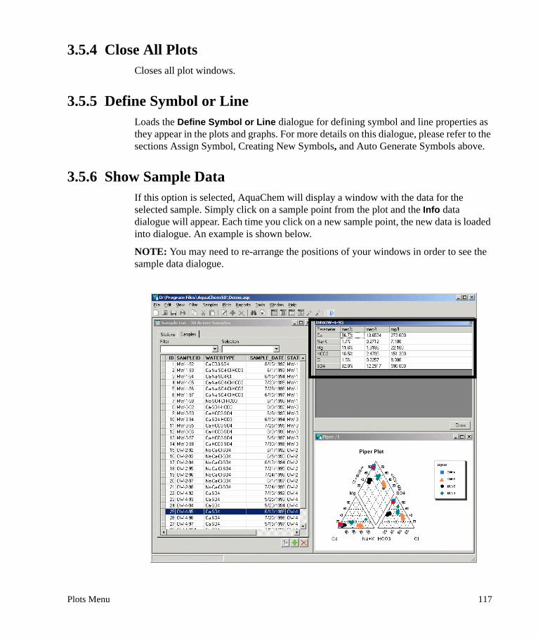
3.5.4 Close All PlotsCloses all plot windows.

3.5.5 Define Symbol or LineLoads the Define Symbol or Line dialogue for defining symbol and line properties as they appear in the plots and graphs. For more details on this dialogue, please refer to the sections Assign Symbol, Creating New Symbols, and Auto Generate Symbols above.

3.5.6 Show Sample DataIf this option is selected, AquaChem will display a window with the data for the selected sample. Simply click on a sample point from the plot and the Info data dialogue will appear. Each time you click on a new sample point, the new data is loaded into dialogue. An example is shown below.

NOTE: You may need to re-arrange the positions of your windows in order to see the sample data dialogue.

Plots Menu 117

3.5.7 Identify Plot DataThe Identify option allows you to link the plotted data to the samples in the active list. This allows you to click on a point in the graph and view the corresponding sample in the active list. This is useful when you have a large number of samples plotted on one plot, and you want to identify outliers.

There are three options available for selecting and identifying points on a plot: None, Selected Plot, and All Plots. The default mode to identify points is on All Plots; this means that all data points on all plots are linked to the database. These three options are described below:

NoneIf you click on a plot, no samples will be highlighted. The data points on the graphs are not linked to the database which means that samples are not identified. When you have several open graphs and a large database with many samples, it may be convenient to have no link between the graphs and the database in order to increase the speed of the various AquaChem operations.

Selected Plot Only the data points in the active graph are linked to the database. The plotted point is activated (turns red color by default) and is selected in the sample list. This mode is useful if you are working with a large data set and want to focus on just one graph.

All plotsThe sampling point of the corresponding sample is activated on all plot windows and on the sample list. If you are working with several graphs, you can simultaneously identify a sample in all plots by clicking near a point in any of the plots, or by clicking on a sample in the active list. The sample will become selected in the active list, and the corresponding data points will be highlighted in red (by default) in all the open plot windows. If the Table view is open, the records will be identified here as well.

3.6 Reports MenuThe Reports allow you to create a summary of your data from your AquaChem database. AquaChem generates seven pre-defined reports and also allows you to create your own report templates.

These reports are all generated in a separate Report window in a spreadsheet view. The reports can be printed ‘as is’ using the [Print] button on the lower-left corner of the window or saved using the [Save] button.

118 Chapter 3: AquaChem Menu Commands

The following is a brief summary of the options under the Reports menu. For more details on Reports, please refer to Chapter 5: Reports.

3.6.1 Compare SampleThe Compare Sample report allows you to compare a sample in your database to another sample or multiple samples. The Compare Sample report uses a linear regression algorithm to generate the Correlation coefficient and the Euclidean distance between a selected sample and all other active samples. Samples having a chemical composition similar to the selected sample will have a correlation close to 1 and a small euclidean distance. Samples having similar chemistry, but being diluted with respect to each other will have correlation close to 1, but a large euclidean distance. Samples with little similarity will have a correlation coefficient close to 0.

3.6.2 Mix SamplesThe Mix Samples report generates solution concentrations resulting from the step-wise mixing of specified proportions of two selected samples from the project database.

3.6.3 Water Quality StandardsThe Water Quality Standards report provides a summary of parameters exceeding the established Water Quality Standards for the selected sample. The selected samples are compared to the pre-defined Water Quality Standards as specified in the Preferences in the File menu.

3.6.4 Rock Source DeductionThis report allows you to determine with what kind of minerals the water sample has been in contact with during its subsurface journey. The results are based on ion ratios and total dissolved solids found in the sample. If results do not meet expectations, they should be confirmed with more a detailed study based on multiple samples, aquifer mineralogy analysis, modeling, and plots.

3.6.5 StatisticsThe Statistics submenu provides several statistical analyses you may wish to perform on your data.

Summary StatisticsGenerates the summary statistics such as Minimum, Maximum, Mean, and Percentiles for all samples available in the project.

Reports Menu 119

Correlation MatrixGenerates a correlation matrix for a specified number of sample parameters that are common to all active samples. A linear regression routine calculates the regression coefficient (r), and the slope and intercept of the regression line.

Trend AnalysisCalculates the trend for a selected parameter using linear regression, Sen’s test, or Mann-Kendall test.

Outlier TestsUses Dixon’s (extreme value) test, Discordance test, Rosner’s test, and Walsh’s test to determine whether there are any outliers for a specified parameter in the dataset.

Tests for normalityUse the Studentized range test (t-test), Geary’s test, Shapiro Wilk test (W test), or Skewness and Kurtosis test to determine if the values for a specified parameter follow normal distribution.

3.6.6 Sample SummaryThe Sample Summary report provides a general overview of a sample including major ions, hydrochemical facies (e.g. Na-Cl), calculated hardness, ion balance, ion ratios, etc.

3.6.7 GeoThermometersThis report displays estimations of the original temperature in the subsurface. This report is an example of a user-defined report and may be deleted if not needed.

3.6.8 IsotopesThis report displays values for common isotopes. This report is an example of a user-defined report and may be deleted if not needed.

3.6.9 Report DesignerThe Report Designer allows you to customize your own reports based on a single sample. The user defined reports may contain any parameter, ratio of parameters or function values. It is also possible to add a template and create a print ready output for your report. For more information refer to Chapter 5: Reports.

120 Chapter 3: AquaChem Menu Commands

3.7 Tools MenuThe Tools menu provides access to the data analysis tools, including converters, calculators, LookUp Tables, and access to the PHREEQC modeling interface. The following is a brief summary of the options under the Tools menu. For more details on Tools, please refer to Chapter 6: Tools.

3.7.1 CalculatorsWhen you access the Calculator option from the Tools menu, you will find the following options:

Aquachem FunctionThe Aquachem Function is a complement to the Calculated parameters tab available in the Sample Details window. It allows you to calculate any function in any available unit quickly and easily, based on the selected sample. The calculations in the Sample Details window are fixed and typically contain only the most commonly used calculations. However, if you want to use some of the other calculations the Aquachem Function dialogue provides these options.

Decay CalculatorThis tool allows you to calculate the degradation of a species by a first order reaction:

You may choose to calculate:

• Concentration after a specified amount of time• Time to reach a specified concentration• Estimate half life from given measurement concentration values

AquaChem includes half-lives for more than 300 species, for physical phases including air, soil, groundwater and surface water. These half-lives are taken from the following reference: Ph. Howard et al. (1991): Handbook of Environmental Degradation Rates.

Find Missing Major IonThis tool helps you to fill in data for missing cations or anions, using the charge balance and existing measured values for other ions for the sample.

AA C

dtdC

-=

Tools Menu 121

Formula Weight CalculatorThis tool helps you to calculate the formula weight based on a user-defined formula.

Volume Concentration ConverterThis converter is used for samples with measured organic chemicals. It allows you to convert measured concentrations in ppm by volume (ppmV), to mg/m3 at a specified temperature.

Special ConversionsThis tool provides conversions for non-linear geochemical calculations. E.g. Conductivity<>Resistivity, pe<>Eh, etc.

Species ConverterThis tool allows you to convert any species into a different form. This is useful to express a measured amount of a parameter as a different aqueous species in mg/L. For example, you may convert Nitrogen as NO3 into Nitrogen as N or vice versa.

Unit CalculatorThis tool performs basic unit conversions for length, time, volume, density, mass, etc.

Calculate faciesThis command calculates the Watertype expression for all highlighted samples.

Corrosion and ScalingThis tool estimates a samples tendency for scaling or corrosion

Oxygen solubilityThis command allows to calculate the theoretic solubility of oxygen based on the temperature and elevations of using the American Society of Civil Engineers’ formula.

3.7.2 QA/QC

Reliability CheckThe Reliability Check report allows you to confirm the validity of the measured sample data. There are a number of tests provided in AquaChem which can provide insight into the reliability of your analysis.

122 Chapter 3: AquaChem Menu Commands

Compare DuplicatesThis report allows you to compare any two records with matching DuplicateID’s and determine where they differ for each concentration result.

Find DuplicatesThe Find Duplicates utility allows you to find and remove duplicate samples or stations:

Simply choose a parameter from the list of available parameters by placing a check mark in the appropriate box. Only Sample Description and Station Description parameters are available. Or to select all parameters, place a checkmark beside Match all parameters. Then click the [Find] button.

AquaChem will then run a query on your database and locate all samples for which the values of the set of specified parameters are identical. Common parameters for this utility are site and date.

The results will then be shown in the lower half of this dialogue. Simply select on the samples you want to remove and press the button to permanently remove these samples from your project database if the duplication was introduced inadvertently.

Highlight Non-detectsSelecting this option will load a dialogue in which you can choose a parameter. Clicking OK in that dialogue will highlight all samples in the Active Samples list that contain a “<“ sign in the selected parameter value.

Tools Menu 123

Highlight outliersSelecting this option will load a dialogue in which you can choose a parameter. Clicking OK in that dialogue will highlight all samples in the Active Samples list that have the outlier flag selected for the parameter value.

Highlight DuplicatesSelect this option in order to highlight all samples marked as duplicates. Aquachem considers a sample as duplicate, if the Duplicate_ID value of the sample description is not empty.

3.7.3 Look Up TablesThe Lookup Tables shows the tables that are defined in the File > Database > LookUp Tables dialogue. These tables allow you to quickly find information for use in AquaChem.

Degradation RatesThis look up table provides a list of degradation rates for common organic chemicals.

PHREEQC PhasesThis look up table provides a list of commonly used minerals including formula and formula weights from the PHREEQC thermodynamic database. If no PHREEQC options are specified in the preferences, then this table will be empty.

Periodic TableThis table provides information for the elements of the periodic table.

Water StandardsThis table contains all of the water quality standards and guidelines for the current database.

LinksThis table contains commonly used reference websites.

Organic CompoundsProvides general information for common organic compounds. This is a user defined table which may be deleted using the File>Database>LookUp Tables dialogue.

124 Chapter 3: AquaChem Menu Commands

Preservation MethodsProvides information for some common methods of sample preservation.

If some tables are unavailable in the Tools menu, use File>Database>Look-up tables to add them. See the Database section later in this chapter for more details.

3.7.4 ModelingAquaChem has a built-in link to the PHREEQC geochemical modeling program, that is capable of creating one or more solutions from the water quality samples in your AquaChem database. The Modeling option under the Tools menu provides links to the various options for PHREEQC. The following is a brief introduction to the modeling features included with AquaChem. For more details, please see Chapter 6 and 7.

Calculate Saturation Indices and ActivitiesThis command will run PHREEQC for the samples selected in your active list. PHREEQC will calculate saturation indices and activities for those parameters which are defined in your database (those parameters listed in the Modeled Parameters tab). The results will automatically be saved back to the Sample Details table, for the selected samples.

Calculate pHThis allows you to calculate the pH for the selected samples. The simulation is based on the assumption that the solution is in equilibrium with a carbonate mineral. This utility may be used to estimate the pH, in the case where a measured pH value is not available. However, this is calculated based on the assumption that the groundwater sample in question flows in a carbonate aquifer and is in equilibrium in respect to calcite or another specified carbonate material.

Calculate EhThis allows you to calculate the Eh for the selected sample based on a redox couple. The Eh is calculated based on the redox speciation, using the Nernst Equation. Each Redox couple gives an individual Eh value which in cases of equilibrium conditions should be reasonable. This menu item launches PHREEQC to search for available redox couples and to calculate ph and Eh values for each couple.

Alk > HCO3, CO3Alkalinity is the measure of the total acid-neutralizing capacity of the water. Since most of the alkalinity in a natural groundwater is due to inorganic carbon species, it can be used to determine bicarbonate and carbonate concentrations. This utility allows to

Tools Menu 125

calculate the bicarbonate and carbonate concentration based on the total alkalinity and pH of a selected sample. For a given alkalinity, the bicarbonate/carbonate ratio increases with higher pH values and decreases under low pH conditions.

When this option is selected, the following warning message will appear:

Click [Yes] to calculate the HCO3 and CO3 modelled values for the selected sample. Any existing HCO3 and CO3 values in the selected sample will be overwritten with the modeled results.

Equilibrate with MineralsThis calculator allows to equilibrate a solution with one or several minerals and calculates the amount of mineral that is necessary to reach equilibrium. This equilibration can be combined with a partial evaporation of the sample to simulation the evaporation process. As a further option, a pump rate and duration can be specified and the program then calculates the total amount of solids, that will be precipitated or dissolved during this period.

PHREEQC (Basic)This allows you to create an input file for PHREEQC, and loads a graphic user interface to the most commonly used features of PHREEQC. The more advanced features (Inverse Modeling, Kinetics, and Advection/Transport) are not included in this option. To utilize these features, you may load one of the USGS’s full versions of graphical interfaces as explained below.

PHREEQC (Advanced)This will load an external window, containing one of the USGS’s PHREEQC interfaces (PHREEQC-Interactive or PHREEQC for Windows). This will allow you to use the full features of the PHREEQC modeling program, using your AquaChem samples as initial solutions.

NOTE: You must have one of the mentioned external graphical interfaces installed and configured in the PHREEQC section of the preferences in order to use this feature.

126 Chapter 3: AquaChem Menu Commands

Generate PHT3D InputThis option allows you to create PHT3D input files for use with PHT3D in Visual MODFLOW versions 4.2 or higher. For more information on this option, please refer to “Generate PHT3D Input” on page 331.

3.8 Window MenuUsing this menu you can arrange the windows in AquaChem master window. Below the Arrange Icons option there is a list of all open windows, so you can easily navigate between them without shrinking them to arrange on a common screen.

Tile VerticalArranges open windows one above the other.

Tile HorizontalArranges open windows side by side.

CascadeCascades open windows.

Arrange IconsOrganizes icons of minimized windows along the bottom of the parent window.

3.9 Help Menu

ContentsDisplays the AquaChem On-line Help.

IndexDisplays the Help index.

AboutDisplays the AquaChem version number and information on how to contact Schlumberger Water Services.

Window Menu 127

This concludes a review of the AquaChem menu items. The following sections describes the components of an AquaChem database.

128 Chapter 3: AquaChem Menu Commands

3.10 The AquaChem DatabaseIn this section, you will find information on the AquaChem database. This includes:

• Parameters• Parameter Groups• Chemicals Master table• Aliases• Lookup Tables• Water Quality Standards• Ranges• Thermometers, and• Calculations

The AquaChem project database files are saved in a Microsoft Access 2000 relational database format. The projects are saved with a unique file extension (.AQC). This is done for two reasons:

1. This prevents any confusion or possible corruption of the file if it were to be accidentally opened in MS Access, and critical changes were made to the data structure or even to the data itself; and

2. This ensures that only AquaChem projects are opened in AquaChem, and that non- supported files that (that could potentially result in corruption or data loss) are not opened.

However, it is still possible to view/edit an AquaChem database file using MS Access. Simply launch MS Access and open this database file, using the File > Open command.

NOTE: It is recommended that you first make a back-up of your database file, before modifying it in the MSAccess environment.

Each AquaChem database relies upon a central database, the Aquachem.MDB database file. This file is a central database that holds information that is common to all databases (e.g. code tables, a set of parameters that can be used to define parameters in a project database, template layouts, etc.). This file is automatically copied to your AquaChem installation folder; the file location and contents should not be modified.

An AquaChem database may contain an unlimited number of samples, depending on the number of parameters it uses and the amount of memory available on your PC. Working with too many samples can slow some operations even though you are only working with a portion of the database. Therefore, working with several databases containing less than 5,000 samples may be more efficient than using one large database.

To view and modify the AquaChem database structure, select File > Database from the main menu while the Samples/Stations list is active. The following dialogue should appear:

The AquaChem Database 129

The Database dialogue contains numerous options for modifying parameters and database settings for your AquaChem database.

At the bottom of the Database dialogue, you will see three buttons:

The Save button will save any changes you make to your database.

The Close button will close the Database options dialogue, and return you to the main AquaChem window.

The Compress button will compress your database. Your project database file size may become large if you have a large number of samples, and are continuously deleting samples. Compressing the database will compact and

repair your database, and may make the file size more manageable. AquaChem will create a backup copy of the uncompressed database file, with the file extension .SAV.

130 Chapter 3: AquaChem Menu Commands

Should you encounter problems with the new compressed file, simply delete this, and restore the previous file by renaming the .SAV file with the extension .AQC.

The Database dialogue contains several tabs. Each tab controls the internal options for the database which include:

• Parameters• Parameter Groups• Chem. Master Table• Aliases• Lookup Tables• Water Quality Standards• Ranges• Thermometers, and• Calculations

3.10.1 ParametersThe Parameters tab allows you to modify the data structure of the current AquaChem database project by adding or deleting parameter fields from each of the four parameter categories. The Parameters tab can also be used to modify the attributes of each parameter (e.g. Display label, Internal name, Molecular weight, Charge, Units, etc.) or to change to order in which the parameters are displayed in the Sample Details window.

In an AquaChem database there are four categories of parameters:

• Station Description Parameters• Sample Description Parameters• Measured Parameters• Analysis Metadata, and• Modeled Parameters

Mandatory parameters are highlighted in yellow. A detailed description of each parameter category follows below:

Station Description ParametersThese are parameters which contain general information about the station. This data is entered once for every individual station. The station can then be assigned to a single sample or multiple samples. Typical parameters for the stations are: station name, ID, location, area, X,Y coordinates, elevation, and well depth. Station Description parameter values can be text or numbers. An AquaChem database may contain a maximum of 255 Station Description parameters.

The AquaChem Database 131

Sample Description ParametersThese are parameters which contain general information about the sample. This category typically includes alphanumeric or data types such as sample ID, sampling date, sampling personnel, etc. Sample Description parameter values can be text or numbers. An AquaChem database may contain a maximum of 255 Sample Description parameters.

Measured ParametersThese are parameters that are either measured at a sampling location (in the field) or derived from a laboratory analysis of a water sample taken from that location. These parameters will contain numerical values for your sample (ex. concentrations for cations, anions, organic contaminants, pH, TDS, etc.). For these parameters, you may enter a comment for every analyzed value as well as an acceptable Range. An AquaChem database may contain unlimited number of Measured parameters.

Analysis metadataIn AquaChem, each measurement may be further described with meta data fields. The initial database includes the most commonly used fields: Method detection limit, Protocol (Method), outlier flag, solubility, and comment. Depending on your field of activity you might want to add meta data fields such as the Practical Quantification Limit (PQL) or the information whether this element has been filtered after sampling. AquaChem allows you to add an unlimited number of meta data fields to the measurement table. Meta data information is only visible in the Sample Detail screen where each parameter appears as an additional column behind the measured value. Note that you have to set the respective to Visible using the Sample Detail Option screen.

Modeled ParametersAquaChem provides an integrated graphical interface for geochemical modeling using PHREEQC where the data for each sample in the database can be used as input data for the PHREEQC simulations. Modeled Parameter values are calculated by PHREEQC during a simulation and read back to the database.

The Modeled Parameters are very similar to numerical parameters, however you may not add comments, description, or define Ranges. Modeled Parameters appear in a separate tab in the Sample Details window.

For more details on the Modeled Parameters and PHREEQC modeling, please refer to Chapter 6: Tools, and Chapter 7: Geochemical Modeling with PHREEQC (Basic).

132 Chapter 3: AquaChem Menu Commands

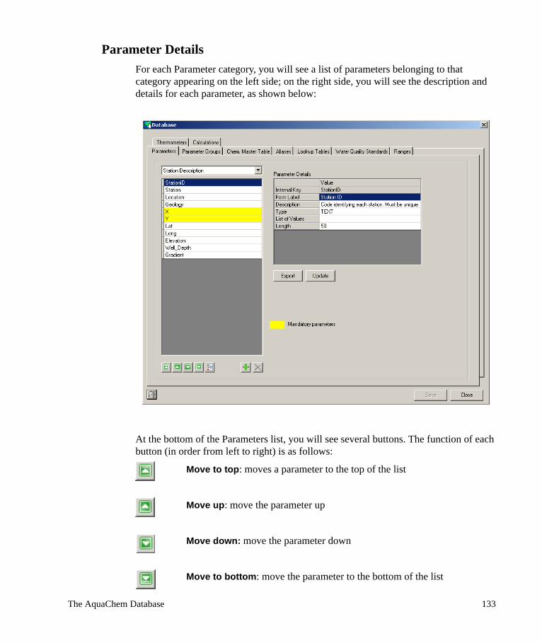
Parameter DetailsFor each Parameter category, you will see a list of parameters belonging to that category appearing on the left side; on the right side, you will see the description and details for each parameter, as shown below:

At the bottom of the Parameters list, you will see several buttons. The function of each button (in order from left to right) is as follows:

Move to top: moves a parameter to the top of the list

Move up: move the parameter up

Move down: move the parameter down

Move to bottom: move the parameter to the bottom of the list

The AquaChem Database 133

Sort alphabetically: sorts parameter list alphabetically

Add new parameter: adds a new parameter

Delete parameter: deletes the selected parameter(s)

Each parameter has a corresponding name, label, and info, so that it can be easily identified in the database, and incorporated in to plots, calculations, and modelling with PHREEQC. Below is a list of the required fields for the various parameter types.

Sample Description Parameters and Station Description Parameters require the following Parameter Details:

• Internal Key• Form Label• Description• Type

One of the new features of AquaChem is the ability to modify the type of the existing parameters for the station and the sample table. Depending on the Type of a parameter, different details need to be provided:

Type Integer, Long, Single, Double:

• Unit• Format

Type Text:

• Length• List of Values (optional)

Type Memo

• Length

Type Boolean and Date:

• No additional parameter details

A Measured Parameter requires the following Parameter Details:

• Internal Key• Form Label• Description• Formula• Formula Weight (g/Mol)

134 Chapter 3: AquaChem Menu Commands

• Solubility• Valence• CAS Registry Number• Unit• Format

A Modeled Parameter requires the following Parameter Details:

• Internal Key• Form Label• Description• Formula• Formula Weight (g/Mol)• Valence• Unit• Format

NOTE: It is not necessary to have values entered for each field for each parameter. However for reports and plots, it is recommended that you enter as much information as possible.

The following is a brief summary of each of these Parameter Details:

Internal Key This is the internal name defined when the parameter is first created; once a parameter has been created, the internal key cannot be changed.

Form Label Display label assigned to the parameter so that it can be distinguished in the Sample/Station Details window, and other AquaChem windows and dialogues.

Description Brief description of the parameter. This information is entered only in this location, and is designed to provide the user with a quick reference. (This field may remain blank if desired).

Length Set the character length of the field

Formula Chemical formula for the parameter.

List of Values Allows you to create a unique pick list for this parameter. To edit the list of values, click the button in the List of Values field. When editing the respective parameter in the sample or station window, only the predefined values can be selected from a combo box.

Formula Weight Formula weight for the measured parameter. For many measured parameters, there is an option to calculate the formula weight

The AquaChem Database 135

(select a measured parameter then you will see a Calculate FMW button appearing below this dialogue. Press this button and AquaChem will automatically calculate the weight of the parameter, provided the formula is entered and available in the database).

Solubility Set the solubility for the measured parameter.

Valence Positive or negative charge (if applicable).

CAS Registry For measured parameters, if you know the CAS (Chemical Number Abstracts Service) Registry number, you can enter it in this field.

Otherwise, you may leave this field blank.

Unit Allows you to select the units that will be applied for the selected parameter (mg/L, meq/L, etc.). For all other parameters without a formula, an editable list of units is displayed. To access this list, simply click in the field beside Unit and press the button to load the list of available units. Note that when changing the unit for a parameter and the database already contains data, existing values are not changed automatically. This change has to be done manually using the Edit > Replace option after saving the database configuration. E.g. when changing the unit for copper from mg/L to ug/l, all copper values have to be multiplied by a factor of 1000.

Format Displays the format for a numerical parameter. This field determines how many decimal places will appear for a numerical parameter. To change the display format, simply click in the field beside Format and press the button to load the Format options dialogue. You can then increase/decrease the number of Decimal places using the up/down buttons or select the Auto or Scientific format for the parameter.

Type Set the parameter data type. There are nine data types in the AquaChem database:

• Boolean• Integer• Long• Single• Double• Date• Text• Memo

The numeric parameter fields do not accept text values such as "ND" or "NA" and will return a value of zero for any such text entry. However, AquaChem does accept "greater than" and "less than" values (e.g. <0.01). In addition, AquaChem allows you to

136 Chapter 3: AquaChem Menu Commands

recognize or ignore the "greater than" and "less than" values on graphs (see the File > Preference > Plots section, and edit the Censored Data options).

The next section will describe how to add new parameters to your database, and create new parameters.

Adding/Creating New ParametersIf you are adding a Station Description or Sample Description parameter to your database, follow the steps below:

• Select File > Database from the main menu (if you have not already done so) and go to the Parameters tab.

• Select the Station Description or Sample Description parameter category from the combo box in the upper left corner of the dialogue.

• Press the button and a New Database Parameter dialogue will appear (as shown on the right-hand side).

• In this dialogue type in the name of your new parameter. This name will be used as the Internal Key, Form Label, and Description for the parameter.

• Click [OK] and this will return you to the list of parameters.• Proceed to fill in the required Parameter Details for this parameter.

If you are adding a Measured Parameter, then follow the steps below:

• Select the Measured Parameters category from the combo box in the upper left corner of the dialogue.

• Press the button and you will see a Parameter List dialogue (as shown on the right-hand side).

• Choose a parameter from the list of available parameters; to add multiple parameters, press the <Ctrl> key (on your keyboard) while you select multiple parameters from the source list. You may use the Find option to run a query for a parameter name to see if it is available in the AquaChem chemical database. Use the combo box above the parameters list to choose from the various measured parameter categories available in AquaChem (Inorganic, Organic, VOC’s, etc.).

The AquaChem Database 137

• Press the [Select] button and the parameter(s) will be added to your database.

If the parameter that you want to add is NOT available in this list, then:

• Click the button (in the lower-left corner of the dialogue) and a New Database Parameter dialogue (as shown to the right) will appear.

• Type in the name of your new parameter (this may be a formula or full chemical name). This name will be used as the Internal Key, Form Label, and Description for the new parameter.

• Click [OK] and you will return to the Database options dialogue.

• Proceed to fill in the required Parameter Details for this parameter.

If you are adding a Modeled Parameter, follow the steps below:

• Select the Modeled Parameters category from the combo box in the upper-left corner of the dialogue.

• Press the button and you will see a PHREEQC Parameters dialogue (as shown on the right-hand side).

• Choose a parameter from the list of available parameters. To add multiple parameters, press the <Ctrl> key (on your keyboard) while you select multiple parameters from the source list. You may use the Find option to run a query for a parameter name to see if it is available in the AquaChem chemical database. Use the combo box at the top of this dialogue to choose from the various parameter categories available in AquaChem (Activities, Saturation Indices).

• Press the [Select] button and the parameter(s) will be added to your template.

If the parameter that you want to add is NOT available in this list, then:

• Click the button (in the lower-left corner of the dialogue) and a New Database Parameter dialogue (as shown to the right) will appear.

• Type in the name of your new parameter. It is important that the name for new modeled parameter matches the names used in the PHREEQC thermodynamic database for phases (minerals) or species. When selected from the list, this will ensure that

138 Chapter 3: AquaChem Menu Commands

the names are matched successfully. This name will be used as the Internal Key, Form Label, and Description for the new parameter.

• Click [OK] and you will return to the Database options dialogue.• Proceed to fill in the required Parameter Details for this parameter.

NOTE: Parameter names should contain numbers and letters only; do not use any other characters, and/or spaces in the parameter names.

Upon returning to the Parameter list, you must then enter the remaining required parameter details including the description, units, formula, format etc. All measured chemical parameters should have a formula weight specified. If you do not know the molecular weight of a chemical parameter, press the Calculate FMW button below the parameter details and AquaChem will read the formula from the field and insert an appropriate molecular weight according to the Periodic Table of Elements. Cations and Anions must be accompanied by their Valence (positive or negative charge).

The Format field is set to Auto by default. To choose a new display format for a parameter, click once in the Format field, and then press the button and you will see the dialogue as shown on the right-hand side.

The Format options allow you to specify the number of Decimal places for measured parameters, and specify if the value will be in Scientific or whole number format. If Auto is selected, then AquaChem will determine the optimal number of decimal places for that parameter. This may result in a “hiding” of a 0 after a decimal place (for example, 7.10 may be displayed as 7.1). To correct this, disable the Auto option, and increase the number of decimals to the desired amount. Once you are finished, press [OK] to accept changes or [Close] to return to the previous dialogue.

Deleting ParametersTo remove a parameter from your database, simply select one or several parameters from the parameters list on the left side of the dialogue and click the button.

Exporting ParametersOn various occasions, it will be useful to save all parameters and respective settings to a file for documentation or review purpose. This may be accomplished by pressing the Export button below the parameter details grid. The information may be saved to in text or Excel format.

The AquaChem Database 139

Update ParametersThe central Aquachem.mdb database holds a master table including hundreds of organic and inorganic chemicals. This is the list you may choose from when adding new parameters to the database. If a parameter has been created manually and the entry misses the formula or formula weight, you may use the Update button to copy the missing information from the chemicals master table to your database parameter. Note that for this the CAS registry number must be filled, since it is internally used for matching parameters. Also, if the parameter does not exist in the Master chemical table, the update process will not return any results.

Mandatory ParametersAquaChem has several parameters which are required for EVERY database, and therefore cannot be deleted from the database. These parameters are needed by various plots, reports, and calculations. Mandatory parameters are highlighted in yellow and when selected, the [Delete] button becomes disabled.

The following is a list of mandatory parameters for an AquaChem database.

Mandatory Sample Description Parameters:

• Sample_Date• SampleID• WaterType

Mandatory Station Description Parameters:

• StationID• X• Y

140 Chapter 3: AquaChem Menu Commands

Mandatory Measured Parameters:

Once you have made changes to the Parameters in your database structure, press [Save] to accept these changes.

3.10.2 Parameter GroupsThe second tab in the Database dialogue is the Parameter Groups tab (as shown below):

Ca HCO3 SAMPLE_DEPTH

Cl K Si

CO3 Mg SO4

COND Na TDS

DENSITY pH TEMP

Eh

The AquaChem Database 141

The Parameter Groups options allow you to sort measured numerical parameters into groups, providing a quick and easy view of specific sample data accessible in the Sample Details window.

For your convenience, AquaChem comes with the following pre-defined parameter groups.

• Show analyzed values only (hides all parameters for which there are no assigned measurement values)

• Anions (e.g. Cl-, F-, SO42-

etc.) • Cations (e.g. Ca2+, Na+, K+, Mg2+, etc.),• Gas (O2, CO2, NO2, etc.)• Isotopes (18O, 2H, 14C, etc.)• Organic Chemicals (BTEX, Vinyl Chloride, etc.)• Overview (pH, TDS, Cond, Major ions)

By selecting a parameter group from the combo box, you can view which parameters belong in a selected group; one parameter may belong to multiple parameter groups. To add/remove parameters from a parameter group, simply select the parameter from either the full list on the left side, or the group list on the right side, and press the or

button to move the parameters accordingly.

You may also create new parameter groups, and add any combination of measured parameters to this new group. This is explained below.

Creating New Parameter GroupsTo create a new parameter group:

• Press the button beside the list of Parameter Groups:• In the Parameter Groups dialogue that

appears, press the button to add a new item.

• Double click on this label and type in a name for this new group. (To delete existing parameter groups, select an item then press the button.)

• Once you are finished press [OK]. • Select this new parameter group from the

combo box listing the available groups. • Use the button to move parameters from

the master list into this group. To move several parameters press the <Ctrl> key while you select multiple parameters from the source list, then press button. To remove parameters from the parameter group, select the target parameter and press the button.

142 Chapter 3: AquaChem Menu Commands

• Once you are finished in the parameter groups dialogue, press [Save] to save the changes and [Close] to return to the main menu of AquaChem.

The parameter groups can now be accessed in the Sample Details window. To do so, open the details for any sample and you should see the following window:

In the Measured parameters tab, beside the Parameter Group label, there is a combo box listing the available parameter groups for the database (indicated by the arrow). Simply choose one of the groups from this list, and AquaChem will display only the data for the pre-defined parameters in that group.

The AquaChem Database 143

3.10.3 Chemicals Master Table

This option allows you to maintain the chemicals master table, which is stored centrally in the Aquachem.mdb file. This table is an extensive list of predefined chemicals, which may be used as templates to create new parameters in the AquaChem project files. You may manually add new parameters, delete parameters, or change fields in existing parameters.

Importing ParametersThe import file typically contains dozens of chemicals that need to be created manually in your database before the respective values can be imported. Often these files have the “one value per row” format as shown below. In this format it is very tedious to extract individual parameter names. The [Import] button allows you to automate the extraction of these parameters and adds them to the chemicals master table and/or the current database parameters. After pressing the [Import] button you will see the following screen:

144 Chapter 3: AquaChem Menu Commands

First, you need to specify the import file by pressing the button. The grid below will be filled with the file contents.

On the Match columns tab you have to match the import file columns to the respective column in the chemicals master table. The CAS number and the parameter name are mandatory.

Press the [Load] button to proceed. This will extract all distinct parameter names found in the specified column and switches the display to the parameters tab. The Parameters

The AquaChem Database 145

tab should now contain the list of extracted parameters as shown below. Each record is preceded by a checkbox, indicating whether this parameter will be imported in the following import procedure.

Press the [Check] button in order to test the parameters for entries having different names but the same registry number. This may be due to a typo in the parameter name, in which case the parameter should be discarded. This can occur as well because of having the same parameter measured in two different ways, e.g. filtered and unfiltered. You might want to add such parameters to the database parameters, but not to the Chemicals Master Tables, which should contain one record per CAS registry number only. The system prompts you when encountering duplicate registry numbers and unchecks the records, if you decide to discard it. Once the parameter check is ended, the Import tab is shown.

This final tab lets you specify if the parameters should be imported to the Chemicals Master Table only or in parallel to the current project database parameters as well. We recommend to import parameters to the Chemicals Master Table only. Then review and complete the parameters with missing formula weight and formula information. Finally,

146 Chapter 3: AquaChem Menu Commands

go back to the Parameters and add new parameters from the updated Chemicals Master Table.

Press the [Import] button to start the import procedure. Note that you will have to confirm the import of parameters where an identical CAS registry number already exists in the target table. If a parameter is to be imported having the same name as a parameter already existing in the target table, this parameter will be simply ignored. At the end of the import process the number of successfully created parameters in the target table will be displayed on the Import tab.

3.10.4 AliasesThe third tab in the Database dialogue is the Aliases tab.

This section allows you to adjust the parameters which are used for some of the internal calculations in AquaChem. Some parameter names have been hardwired to AquaChem for these calculations. For example, in order to calculate the hardness given by the sum of Ca and Mg, AquaChem must know if these parameters are called Ca or CALCIUM in the database.

The AquaChem Database 147

Mandatory aliases which require to have an assigned parameter are highlighted in yellow. Aliases that have a white background may stay unmatched, however, certain functionalities may not be available. e.g. if the 18O and Deuterium aliases are not defined, the meteoric waterline plot and isotope related calculations will not be active, even if the respective parameters exist in the database.

For most purposes, it is recommended not to modify the original parameter names. However if you must rename a mandatory parameter, this section gives you the opportunity to map the database field to the parameter name in the database. An important alias is the “Measured Alkalinity”. Often carbonate species are measured in the field as alkalinity and expressed in mg/l CaCO3. If this is the case, then the respective parameter must be matched to the Measured Alkalinity alias. After that, the electroneutrality calculation will be based on alkalinity rather than HCO3 and CO3 concentrations. Alkalinity may be plotted on Piper diagrams and PHREEQC will use this parameter when modeling the aqueous species distribution. After setting the measured alkalinity alias, make sure you return to the respective parameter and select the appropriate unit, as alkalinity units (mg/l CaCO3, french degrees, german degrees, meq/L), differ from all other concentration units (mg/l, mmol/l etc.).

When you are dealing with very alkaline water samples and your data contains measured hydroxide concentrations, make sure that the “Hydroxide” alias is matched to the respective parameter since it is used for the alkalinity calculation.

Once you are finished in the Aliases tab, press [Save] to save any changes and [Close] to return to the main menu.

3.10.5 Lookup TablesThe next tab in the Database dialogue contains options for Lookup Tables, as shown below:

148 Chapter 3: AquaChem Menu Commands

Lookup tables allow you to integrate any type of information in tabular format to the AquaChem Environment which may be helpful for your work. This can be a list of projects, customers, or a table with properties of organic contaminants. These tables are created in the Microsoft Access environment. It is recommended that the table names start with LUT (Lookup Table) for the naming convention, (e.g. LUT_organics). Then create a view of this table that orders the data the way you want it to show up in the table in AquaChem. The respective view must start with the letters LUV (Lookup Views) in order to be detected by AquaChem.

On the left side of this dialogue, you will see Available Tables which contains a list of all views starting with LUV that are not already integrated into AquaChem. Pressing the button adds the view to the right-hand grid of Selected Tables. The Menu Option is the name of the entry as it will appear under the Tools > Lookup Tables menu in AquaChem. The Description field lets you add a description to the table.

Use the and buttons to order the tables.

The AquaChem Database 149

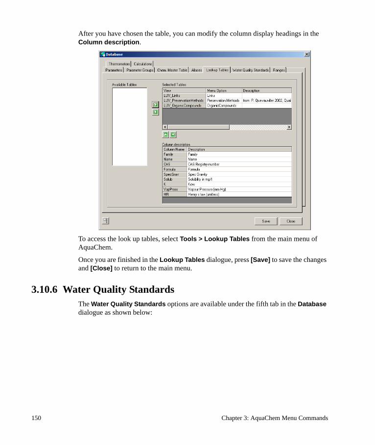
After you have chosen the table, you can modify the column display headings in the Column description.

To access the look up tables, select Tools > Lookup Tables from the main menu of AquaChem.

Once you are finished in the Lookup Tables dialogue, press [Save] to save the changes and [Close] to return to the main menu.

3.10.6 Water Quality StandardsThe Water Quality Standards options are available under the fifth tab in the Database dialogue as shown below:

150 Chapter 3: AquaChem Menu Commands

The options in this dialogue allow you to view and modify water quality standard levels, and create new sets of standards. These standards are used in the data analysis reports, table views, and individual sample details. Measured parameters which exceed these pre-defined levels are highlighted in predefined colors depending upon the specified preferences. This allows you to quickly identify sample exceedances and water samples which may be harmful to humans and the environment.

To view the available standards, simply choose a standard from the combo box beside the Water Quality Standard field. To view a guidline level for the selected guideline, simply choose a level from the combo box beside the Level field.

Standards can be modified by simply editing the existing values beside each parameter in the grid, or importing a complete set of standards from a file (*.txt or *.xls). For each parameter in the database you may define up to three guideline levels.

To view the properties of a Water Quality Standard, press the button beside the Standard name, at the top of this dialogue. You should then see the following dialogue:

The AquaChem Database 151

In this dialogue, you may view and/or modify the Standard Name, Reference, and Year Approved. It is useful to provide a URL to the original standard so that you can check from time to time whether there have been changes made to the standard. The Levels frame lists the defined guideline levels and their corresponding colors. You can add a new level by clicking the button .

You can have an unlimited number of levels for the selected guideline. However, In most cases, two levels will be adequate (Tolerated level, Guideline level). Simply add the number of levels appropriate for the guideline. You may then assign a name to each level (Tolerated level, Guideline level, cleanup level etc.). You can call the first level MCL (applicable in U.S.), or you can name this MAC (applicable in Canada). Simply type in the new name in the appropriate field. Similarly, for Level 2 and Level 3 you may enter your own labels.

For your convenience, three commonly used Water Quality Standards are included with AquaChem:

• World Health Organization (WHO) - Guidelines for Drinking Water Quality - 3rd Edition - 2004

• U.S. Environmental Protection Agency (US EPA) - National Primary Drinking Water Regulations (EPA 816-F-02-013, July 2002).

For your reference, these guidelines are also available in spreadsheet view, and included in your AquaChem installation folder. In addition, the following Water Quality Standard is provided with your installation, and can be imported into AquaChem:

• US EPA - National Secondary Drinking Water Regulations (EPA 810/K-92-001, July 1992)

• Canadian Council of Ministers of the Environment (CCME )- Canadian Environmental Quality Guidelines - 2002

• Health Canada - Guidelines for Canadian Drinking Water Quality - 2004

152 Chapter 3: AquaChem Menu Commands

For more details on these standards, please see the website links below:

WHO: http://www.who.int/water_sanitation_health/dwq/gdwq3/en/

CCME: http://www.ccme.ca/publications/can_guidelines.html

US EPA http://www.epa.gov/safewater/mcl.html

Health Canada http://www.hc-sc.gc.ca/hecs-sesc/water/dwgsup.htm

NOTE: The Water Quality Guidelines tab in the Database is used to edit the guidelines available to the project. To select which guidelines are used in the project use File>Preferences. To specify which Water Quality standard should be used for your database, you may do so in the Preferences dialogue, available under the File menu. Select the General tab, and in here you will be presented with a combo box displaying the available Standards.

If the above mentioned standards are not sufficient for your project needs, you may create a new set of standards, as explained in the following section.

Creating New Water Quality StandardsTo create a new water quality standard, follow the steps below:

• If you have not already done so, open the Database options dialogue (File > Database), and select the Water Quality Standards tab.

• Press the button (in the upper right corner) to access the Water Quality Standards properties dialogue, as shown below.

• Click the [New] button to create a new standard

The AquaChem Database 153

A blank Water Quality Standards dialog will load (shown above). Here you can:

• Enter the name for this new set of standards• Enter a reference for the new set of standards• Enter a URL for the set of standards• Enter the year that the standards were approved• Enter guideline levels for the new set of standards (see above for more

information)• Once finished, click the [Close] button.

Under the Water Quality Standards tab, select the new standards from the Water Quality Standards combo box (shown in the image below). Below that, select a guideline level from the Level combobox.

154 Chapter 3: AquaChem Menu Commands

There are two ways to enter parameters and assign guideline levels: the values can be entered manually or the data can be imported from a file. Either way, data is entered for one guideline at a time.

Adding Data Manually

To manually add guideline levels, simply click on the button. A new field will be added to the grey grid, where you can manually enter the following data:

Type User specified acronym that allows to group parameters, e.g., in chemicals (C), microbial (M) and radionuclide (R) parameters

Parameter* Parameter name in guideline

CAS# CAS registry number (for simplified parameter matching)

Unit Original parameter unit. This may differ from AquaChem’s internal unit. The value used in AquaChem may need to be converted.

Standard* Maximum value or interval for guideline

Comment A comment

Year The year when the standard was introduced or revised

The AquaChem Database 155

*Mandatory Fields

Importing a Guideline Level

For importing guidelines, an excel file (or text file) must be created for every guideline level, e.g., MCL, MCL goal, etc. The column structure in the excel file must exactly match the column format below, however all columns may be empty except the parameter and standard (Upper_Limit) column.

It is recommended that the parameter names in your file are identical to the respective parameter names (the Internal Key name) in the AquaChem database template. If the parameter names are different, AquaChem will not recognize the data for these parameters when you attempt to import them, and you will need to match the fields manually. Optionally, the standard to be imported may contain the CAS registry number per substance, allowing to match this unique code against the CAS registry numbers for the database parameters resulting in a more efficient detection of parameters.

NOTE: Do not include headers in the text file. The first line in your text file should be the first available parameter for which you have a guideline level.

To import the water quality standards using a text or excel file:

• Click the button beside the Import water quality standards from File field for the filename. The following dialogue will then appear:

• Locate the source file on your computer, then click [Open].• After you load the file, the dialogue will be refreshed similar to the one shown

below:

156 Chapter 3: AquaChem Menu Commands

• The grid is divided into two sections: grey fields and white fields. The grey fields represent the original (raw) water quality standard data that was imported. The adjacent white cells represent the matched AquaChem parameters and the corresponding standard levels. The standard values may be adjusted for differences in units between AquaChem and the original source file.

• AquaChem will attempt to identify matching parameters in the database either by using the CAS number if available, or the parameter name. You should carefully scan the list and verify if all the parameters have been identified, e.g. the original name in the guideline may say “Total Dissolved Solids” while the database parameter may say TDS. This will not be discovered by AquaChem and you must select the corresponding AquaChem parameter.

• To manually assign an AquaChem parameter to a standard record, simply click the cell and select a parameter from the combobox (shown below)

The AquaChem Database 157

• If the original standard is expressed in mg/l but AquaChem uses ug/l for the same parameter, a conversion factor of 1000 is automatically applied for the value used in AquaChem to check for exceedances. However, for some parameters such as Nitrate and Silica, the parameters may be expressed in different formulas, e.g., nitrate originally as N and AquaChem may express nitrate as NO3. In these cases, a conversion factor must be calculated manually and applied to the standard in AquaChem. For example, if the original standard for nitrate as N is 10, then the standard in AquaChem for nitrate as NO3 is 44.2. You can use the species converter to calculate the conversion factor.

To use this new standard, you must select this in the File > Preferences dialogue, under the General tab.

Once you are finished in this dialogue, press [Save] to save the changes and [Close] to return to the main menu.

3.10.7 RangesThe next tab in the Database options is the Ranges tab, as shown below:

158 Chapter 3: AquaChem Menu Commands

Ranges are similar to the drinking water standards; they allow you to define qualitative and quantitative intervals for any parameter. An example for Conductivity (cond) is shown in the dialogue above, and detailed below:

Conductivity (uS/cm)

100-1000 natural aquifer range

<250 low salinity (C1)

250-750 medium salinity (C2)

750-2250 high salinity (C3)

>2250 very high salinity (C4)

Data can be marked as a “Natural Occurrence” using the provided check-box. If a natural occurrence range is defined for a parameter, the reliability check tool will later be able to detect all concentrations outside this interval. The natural for a parameter occurrence depends strongly of the type of water you are analyzing. It will be very different whether you are working on surface water, ground water or sea water. Please review the values included in the startup database and adjust them to whatever value is applicable in your study area.

Ranges can be useful for interpreting stable isotope data: S, N, C, Sr, He. Isotopes reflect the signature of their source. If the ranges of every potential source is given, an analyzed value can be easily attributed to one of the sources.

Creating a New RangeTo add a new Range item:

• Choose the desired parameter from the combo box at the top of this dialogue.• Press the button to add a new item.• Enter the desired Label (descriptive name or text).• Enter the corresponding Minimum and Maximum values.• Check the Natural Occurrence box if needed.• Press [Save] to save the changes and [Close] to return to the main menu.

To view the range options for a sample, load a Sample Details Window and then right-mouse click on the parameter name. A dialogue titled Parameter Details appears, showing all the information about this parameter including the ranges.

The AquaChem Database 159

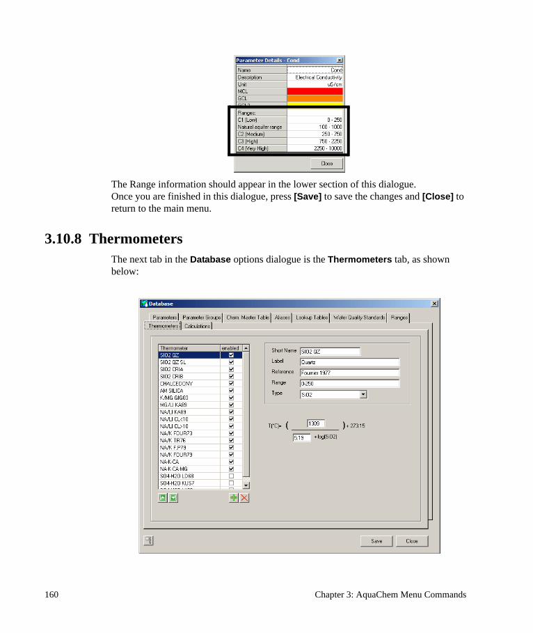
The Range information should appear in the lower section of this dialogue. Once you are finished in this dialogue, press [Save] to save the changes and [Close] to return to the main menu.

3.10.8 ThermometersThe next tab in the Database options dialogue is the Thermometers tab, as shown below:

160 Chapter 3: AquaChem Menu Commands

The Thermometers options allow you to modify existing Geothermometers or to create new ones. Geothermometers are used to estimate the original subsurface reservoir temperature of ascending groundwater which underwent conductive cooling during its ascent. They reflect the temperature dependence of most rock-water reactions. The reactants, which remain dissolved during the journey to the surface, are ideally proportional to their original aquifer temperatures. For example SO2 (Quartz or Chalcedony dissolution or Na/K for albitisation). The original reference and the temperature range for which the thermometer is valid (most thermometers only work above 100 °C) and can be viewed and edited in this dialogue.

Geothermometers are generally derived from the Van't Hoff equation and have the form:

where

a and b are constants describing a straight line in the 1000/T-log(K) plot, and

K depends on the reaction used for the geothermometer (SiO2 for all SiO2 thermometers, Na/K for the Na/K thermometer, etc.)

Since thermometers are usually developed from empirical data, different coefficient values are found in the literature. AquaChem includes a compilation of most currently used geothermometers as shown in the figure above. The equations for each of the thermometers are stored in the project database file and can be customized and modified. Each thermometer record includes the formula’s coefficients, the reference (author and year), and the range within which the formula was calibrated.

The Thermometers tab contains a list of available geothermometers that can be plotted on a geothermometers plot. If a thermometer is enabled (checked) it will be available for the geothermometers plot. If it is disabled (not checked) it will not be available for the geothermometers plot.

There are several fields for each thermometer:

• The Short Name refers to the list name of the selected geothermometer.• The Label refers to the reference name of the geothermometer. • The Reference refers to the author and year of the original publication.• The Range refers to the temperature range within which the thermometer is

supposed to provide reliable data. This normally corresponds to the range of the calibration data.

• The Type refers to the thermometer class.

T C( )a

b K( )log+--------------------------⎝ ⎠⎛ ⎞ 273+=

The AquaChem Database 161

Creating a New GeothermometerYou may add published thermometers from literature or create your own thermometer if the formula structure corresponds to one of the pre-defined thermometers provided by AquaChem.

For example, to create a new Na/K thermometer:

• Select an existing Na/K geothermometer,• Click the button to create a new Na/K geothermometer (new thermometer

will be added to the bottom of the list).• Select the new geothermometer Type.• Enter a new Short Name, Label, Reference, Range, and Type.• Replace the formula parameters from the original geothermometer with the

parameters from the new geothermometer.• Press the [Save] button to save the changes to the database.

This new thermometer is automatically included in thermometer calculations and can be visualized as a Geothermometer Plot.

Once you are finished in the Thermometers section press [Close] to return to the main menu.

3.10.9 CalculationsThe last tab in the Database options dialogue is the Calculations tab, as shown below:

162 Chapter 3: AquaChem Menu Commands

The Calculations tab allows you to set the equation coefficients and parameters that are used in the isotope and geothermometer calculations. It also provides information on the various calculations that are performed by AquaChem.

Isotopes In the Isotopes frame, you may define coefficients for several functions for the isotopic calculations. With the exception of the meteoric water line, all equations have a highly regional character. If you want to make temperature or precipitation estimations, please find the respective coefficients for your study area. There are also parameters for 18O (Oxygen 18) and 2H (deuterium) equations: meteoric waterline, altitude-isotope and altitude-mean annual temperature relations. All of these functions are derived empirically. The coefficients for the isotope-altitude and the isotope-temperature functions are regional and should be used only in the area of calibration. Indicate the area of application of these functions in the field provided.

Geothermal GradientThe Geothermal Gradient is used for a simple subsurface temperature estimation. These options allow you to specify which values are used to calculate the temperature at a given depth. The geothermal gradient is used in the geothermometer plot. It allows the user to estimate the subsurface temperature of waters produced by a borehole if the

The AquaChem Database 163

depth of the inflow zone is known. This temperature is then compared to geothermometer temperatures for the respective sample.

The formula for the Geothermal Gradient calculation is as follows:

The subsurface temperature [T (z)] = Average surface temperature + geothermal gradient * depth (km).

The geothermal gradient may vary regionally; it is approximately 33 °C/km in most environments. Any changes made to the Geothermal gradient equation should be registered with AquaChem by pressing the [Save] button prior to closing the Database options dialogue.

Water Type (major ion definition)First you may choose between an long and short name for water facies calculation. For the long version of the water type, the water type expression is calculated as follows:

• All concentrations are converted to meq/L.• Values are then transformed from meq/L to meq%.• All parameters which are below a certain limit (10% by default) are removed.• The remaining ions are considered Major ions. These ions are ordered

according to their percentage. Cations are ordered first, followed by the anions.• The result is the WaterType string (e.g. Ca-Mg-HCO3).

The threshold for determining if an ion is major is normally 10%; however in some countries 12.5% is more common. the higher the threshold, the smaller number of parameters that may exceed this threshold is. Usually, only major ions (Na, Ca, Mg, HCO3, Cl, SO4) will have a concentration that allows them to exceed the defined threshold. If you want to make sure, that other important elements such as potassium or nitrate appears in the water type expression, then you can achieve this by lowering the threshold value.

The second (short) way of calculating the water type consists of simply listing the most frequent cation and the most frequent anion, which results in one of the following combinations for most natural waters: Ca-HCO3, Ca-Cl, Ca-SO4, Na-Cl, Na-SO4, Na-HCO3.

The water type is displayed in the Sample Details window as a distinct parameter.

NOTE: The Water Type parameter cannot be edited; it is read-only. Also when changing the type of water type expression or when changing the threshold value for major ions, you must recalculate the water type expressions for all samples using the Tools>Calculators>Calculate Facies menu item.

164 Chapter 3: AquaChem Menu Commands

FunctionsThe Functions frame lists all of the internal calculations performed by AquaChem, with reference information for each calculation provided in the fields below. All of the active functions (as indicated by a checkmark) will be available as database parameters which can be included in statistical comparisons and for plotting data. In this dialogue, you may select which calculations should appear in the function lists. For example, if you never use the enthalpy calculation, you may deactivate it here. In addition, you may define the default units for some of the functions.

The calculated values are displayed in the Sample Details window, under the Calculated tab:

The functions such as hardness, ion balance, etc. are hardwired to AquaChem; as such, it is not possible to change the parameters involved in these calculations. You may however, edit the name of the function or activate/deactivate a function. Deactivated functions will not appear in the list of functions within AquaChem. For functions that can be expressed in different units (e.g. hardness as °f, °g, mg/L CaCO3) you may specify the default unit.

To edit the name of the function, press View > Options when the Sample Details window is active, and edit the options under the Functions tab.

AquaChem includes a number of common calculations for determining common geochemical parameters. Each of the available calculations (functions) is explained below.

Calculated Alkalinity

Acid neutralizing capacity. Generally equal to the concentration of 2CO32- + HCO3

- +OH--H+.

The AquaChem Database 165

Calculated Density

Calculated density based on the partial molal ionic volumes. This value is calculated as follows:

where

v is the molar volume: ,

ni is the concentration in mmol/l of ion i and,

vi is the partial molar volume at

Partial molal ionic volume coefficients are from Owen and Brinkley, 1941 and for more details, see Hounslow, 1995, p. 58

Calculated TDS (Total Dissolved Solids)

TDS is a measure of the evaporation residue at a given temperature. It can also be thought of as the mass of all ions. It is important to note that the calculated TDS is only an approximation and it is always better to have a measured value. TDS is calculated as follows:

First the sum in mg/L of Na+K+Mg+Ca+Cl+SO4 is calculated. Then AquaChem checks if (Ca+Mg-SO4) > (HCO3+CO3). This is done because TDS is not simply the sum of ions but the weight of residue you would expect if you evaporate the entire sample. In waters that contain an excess carbon (Ca+Mg-SO4) < (HCO3+CO3) you may not add all carbon to the residue since bicarbonate will partly outgas as CO2 during evaporation. Only the quantity of HCO3 which can be precipitated as calcite and dolomite is added to the estimate of the TDS. SO4 is deduced from Ca+Mg because gypsum is built first and the Ca that is used up by this process cannot be used any more to build calcite. If (Ca+Mg-SO4) > (HCO3+CO3) then all HCO3 and CO3 can be added to the TDS because there is enough Ca+Mg to build calcite and dolomite.

Total Hardness

The sum of ions that can precipitate from water as calcite or dolomite. Generally, the sum of Ca and Mg, expressed in meq/L or mg CaCO3/L, or in degrees.

100 mg CaCO3/L = 1 mmol Ca2+/L = 2 meq Ca2+/L

The Degrees equivalents are as follows: 1 German Degree = 17.8 mg CaCO3/l

D1000 v– TDS

1000------------+

1000--------------------------------------------=

v S ni vi( )=

25 C

166 Chapter 3: AquaChem Menu Commands

1 French Degree = 10 mg CaCO3/l

Non Carbonate (Permanent) Hardness:

Parts of Ca and Mg in excess of HCO3.

Carbonate (Temporary) Hardness:

Parts of Ca and Mg which are balanced by HCO3 and thus can precipitate as CaCO3.

Residual Sodium Carbonate (RSC)

The RSC has the following equation: RSC=(CO3-+HCO3

-)-(Ca2++Mg+2)

It is similar to the SAR in that it expresses the sodium content in relation with Mg and Ca. This value may appear in some water quality reports although it is not frequently used. If the RSC < 1.25 the water is considered safe If the RSC > 2.5 the water is not appropriate for irrigation.

Langelier Saturation Index (LSI)

The Langelier index is a popular way of expressing the equilibrium state of a solution in respect to calcite.

• Index between -0.5 and +0.5: the water is balanced • Index < -0.5: the water is Corrosive. • Index > +0.5: the water is scale forming.

LSI = pH - pHswhere pH is the measured pH and pHs is the pH where the water sample would be in equilibrium. The pHs is estimated from temperature, alkalinity, hardness and total dissolved values.

pHs = (9.3 + a + b) - (c + d)

a = log(TDS) - 1) / 10

b = -13.12 * log(temp + 273.15) + 34.55

c = log10(Ca as CaCO3) - 0.4

d = log(Alkalinity)

Note that the LSI is only an approximation of the real saturation state. Whenever possible you should use the PHREEQC modeled saturation index of calcite or dolomite in your studies.

The AquaChem Database 167

Ryznar Stability Index (RSI)

The Ryznar stability index (RSI) attempts to correlate an empirical database of scale thickness observed in municipal water systems to the water chemistry. Like the LSI, the RSI has its basis in the concept of saturation level. Ryznar attempted to quantify the relationship between calcium carbonate saturation state and scale formation. The Ryznar index takes the form:

RSI = 2(pHs) - pH

The empirical correlation of the Ryznar stability index can be summarized as follows:

• RSI << 6 the scale tendency increases as the index decreases. • RSI >> 7 the calcium carbonate formation probably does not lead to a

protective corrosion inhibitor film.• RSI >> 8 mild steel corrosion becomes an increasing problem.

ElectroNeutrality

(Cations - Anions)/(Cations + Anions), expressed as a percent. The Electro Neutrality is a common quality control method.

Sum of Anions:

Sum of all measured anions for the sample, in meq/l.

Sum of Cations:

Sum of all measured cations for the sample, in meq/l.

Sum Ions:

Sum of all ions in your sample. This can be expressed in mmol/l, meq/l, mg/L.

Exceeds_Lev1, Exceeds_Lev2, Exceeds_Lev3

The functions “Exceeds_Lev1, Lev2, Lev3” returns “-1” for samples which contain at least one concentration exceeding the specified water quality standard and they return 0 if no concentration has been exceeded. It is a convenient way of finding samples which should be verified and analyzed more carefully. This is especially effective if you are dealing with many different parameters that might exceed the guidelines.

SAR (Sodium Adsorption Ratio)

The sodium adsorption ratio is an important water quality criterion for irrigation waters. It is used in the Wilcox plot.

168 Chapter 3: AquaChem Menu Commands

NOTE: The concentrations used in the formula are in meq/L.

MH (Magnesium Hazard)

Magnesium is considered to be harmful for plants, but the effect is reduced by the presence of calcium. Magnesium Hazard was proposed by Szabolcs and Darab (1964).

Units are in meq/l. MH > 50 is considered to be harmful for irrigation water.

NOTE: The Concentrations used in the formula are in meq/L.

Calculated TOC

This function calculates the total carbon within all organic species. Carbon from inorganic species such as HCO3, CO3, CO2 is not included.

Calculated TOX

Calculated total organic halogens. Sum of all halogens (e.g. Cl-, Br-, I-, etc.) present in ug/L, mg/L or g/L in all organic parameters (thus, Cl from Cl- or CL2 is excluded).

z(18O)

Average infiltration height as a function of oxygen 18 isotopic composition. Coefficients are valid only for a very limited zone, and must be established for your area of interest using empirical data.

T(18O)

Average temperature of infiltration zone as a function of oxygen 18, isotopic composition. Coefficients are valid only for a very limited zone, and must be established using empirical data.

SAR NaCa Mg+

2----------------------⎝ ⎠⎛ ⎞ 0.5---------------------------------=

MH MgCa Mg+( )

-------------------------- 100·=

The AquaChem Database 169

T(2H)

Average temperature of infiltration zone as a function of deuterium. Coefficients are valid only for a very limited zone.

z(2H)

Average infiltration height as a function of deuterium. Coefficients are valid only for a very limited zone.

Temperature (Z)

Estimated Temperature for a given depth and geothermal gradient.

Temp > H H2O (l)

Enthalpy of liquid water as a function of temperature (t). This is a polynomial function:

Temp = enth(water)

value! = a(1) + a(2) * t + a(3) * t ^ 2 + a(4) * t ^ 3 + a(5) * t ^ 4 + a(6) * t ^ 5 + a(7) * t ^ -1 + a(8) * t ^ -2 + a(9) * log10(t)

where

a(1) = 418.84

a(2) = 10.286

a(3) = -0.05092

a(4) = 0.00026309

a(5) = -0.00000069303

a(6) = 0.00000000074566

a(7) = -1209.8

a(8) = 11.99

a(9) = -353.76

For more details please refer: Fournier & Potter, 1972.

Temp > H H2O (v)

Enthalpy of water vapor as a function of temperature. This is a polynomial function:

Temp = enth(water vapor)

170 Chapter 3: AquaChem Menu Commands

enthalpy = a(1) + a(2) * t + a(3) * t ^ 2 + a(4) * t ^ 3 + a(5) * t ^ 4 + a(6) * t ^ 5 + a(7) * t ^ -1 + a(8) * t ^ -2 + a(9) * log10(t)

where

a(1) = 2035

a(2) = -5.0499

a(3) = 0.057399

a(4) = -0.00030426

a(5) = 0.00000079095

a(6) = -0.00000000086968

a(7) = 1342.4

a(8) = -13.298

a(9) = 396.29

For more details please refer: Fournier & Potter, 1972:

SiO2 > H H2O (l)

Enthalpy of liquid water as a function of dissolved silica. This is a polynomial function:

enth = a(1) + a(2) * SiO2 + a(3) * SiO2 ^ 2 + a(4) * SiO2^ 3 + a(5) * log10(SiO2)

where

a(1) = -42.198

a(2) = 0.28831

a(3) = -0.00036686

a(4) = 0.00000031665

a(5) = 77.034

For more details please refer: Fournier & Potter, 1972:

SiO2 > H H2O (v)

Enthalpy of water vapor as a function of dissolved silica. This is a polynomial function:

enth = a(1) + a(2) * SiO2 + a(3) * SiO2 ^ 2 + a(4) * SiO2^ 3 + a(5) * log10(SiO2)

The AquaChem Database 171

where

a(1) = -3.5532

a(2) = 0.146

a(3) = -0.0004927

a(4) = 0.0000012305

a(5) = -0.00000000049421

For more details please refer: Fournier & Potter, 1972:

Exceeds_Lev1, Exceeds_Lev3, Exceeds_Lev3

These functions return true (-1) for all samples, where at least one parameter exceeds the respective standard level (1 2 or 3). This function is convenient when used in a query expression. If you query for exceeds_lev1 = -1 then all samples having values exceeding the first level of the current water standard will be highlighted in the sample list.

Exceeds_Solubility

Returns “true” (-1) if solubility is exceeded and the solution is includes a chemical which solution is above the specified solubility.

Exceeds_NO

Returns “true” (-1) if natural occurrence is exceeded by one of the measured concentrations. The natural occurrence range can be defined in the database screen on the range tab.

Season

Returns the season number for the sample (i.e. 1=Spring, 2=Summer, 3=Fall, 4=Winter - based on Northern Hemisphere seasons). Note that this is a convenient way to find and select all samples that were sampled in the same season but in different years.

• Spring: 21/3 - 20/6• Summer 21/6 - 20/9• Fall 21/9 - 20/12• Winter 21/12 - 20/3

On the southern hemisphere as defined in the preferences screen: 1=Fall, 2 equal Winter, 3=spring, 4=Summer

172 Chapter 3: AquaChem Menu Commands

Month

Returns the month for the sample (i.e. 1=January, 2=February, etc.). Again, using this function in the find screen might be convenient to select data for calculating month based statistics over several years.

Year

Returns the year for the sample.

Once you are finished in the Calculations section, press [Save] to save the changes and [Close] to return to the main menu.

The calculated parameters are treated by AquaChem as regular database parameters with respect to plotting, searches, or statistical calculations. However, in order for the built-in calculations to work, their corresponding database parameters must be included in the database. For example, the database must include Ca and Mg in order to calculate hardness, and both of these parameters must be identified with an Internal Name of ‘Ca’ and ‘Mg’ respectively.

NOTE: If your database does not include some of the required parameters or if some of the required parameters are not properly mapped in the Alias section, then the applicable function(s) requiring these parameters will contain null values or erroneous information.

The AquaChem Database 173

174 Chapter 3: AquaChem Menu Commands

4Plots

When you select Plots from the main menu and then New, a sub menu will appear with a list of the twenty three (23) available plot types:

• Box and Whisker (Time)• Box and Whisker (Multiple Parameters)• Box and Whisker (Multiple Stations)• Depth Profile• Detection summary• Durov Plot• Geothermometer Plot• Giggenbach Triangle• Histogram• Ludwig-Langelier Plot• Map Plot• Meteoric Water Line (MWL) Plot• Pie Plot• Piper Plot• Probability Plot• Radial Plot• Scatter Plot• Schoeller Plot• Stiff Plot• Ternary Plot• Time Series (Statistics Summary)• Time Series Plot (Multiple Parameters)• Time Series Plot (Multiple Stations)• Wilcox Plot

AquaChem allows you to create multiple plots for the same data set and view these plots simultaneously within the Windows environment. Each of these plots is explained

175

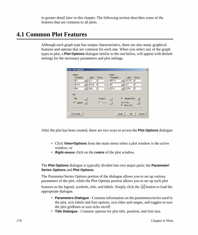
in greater detail later in this chapter. The following section describes some of the features that are common to all plots.

4.1 Common Plot FeaturesAlthough each graph type has unique characteristics, there are also many graphical features and options that are common for each one. When you select any of the graph types to plot, a Plot Options dialogue similar to the one below, will appear with default settings for the necessary parameters and plot settings.

After the plot has been created, there are two ways to access the Plot Options dialogue:

• Click View>Options from the main menu when a plot window is the active window; or

• Right-mouse click on the centre of the plot window.

The Plot Options dialogue is typically divided into two major parts: the Parameter/Series Options and Plot Options.

The Parameter/Series Options portion of the dialogue allows you to set up various parameters of the plot, while the Plot Options portion allows you to set up such plot features as the legend, symbols, title, and labels. Simply click the button to load the appropriate dialogue.

• Parameters Dialogue - Contains information on the parameters/series used in the plot, axis labels and font options, axis titles and ranges, and toggles to turn the plot gridlines or axis ticks on/off.

• Title Dialogue - Contains options for plot title, position, and font size.

176 Chapter 4: Plots

• Symbols Dialogue - Contains options for symbols used in the plot, proportional symbol options, etc.

• Legend Dialogue - Contains options for displaying a plot legend, legend title, and display features.

• Labels Dialogue - Contains options for displaying and customizing symbol labels.

• Format (Axis) Dialogue - Contains options for customizing the axis values and appearance.

Each Options dialogue has the following buttons located at the bottom of the dialogue:

The [Apply] button will apply the current plot settings to the selected plot type.

The [OK] button will apply the current plot settings to the selected plot type and will close the plot options dialogue.

The [Cancel] button closes the plot options dialogue.

The [Set Default] button will save the current plot settings as defaults for that plot type. This includes plot parameters, grid lines, interval, axes titles, legend appearance and symbol settings, but does not include plot titles. The default settings will be applied every time you create a NEW plot of that type, with the current database.

The Axes/Parameters dialogue has several buttons and functions which are common for most (but not all) plot types:

The add button allows you to add new parameters to the plot. The add button will load the parameter list dialogue, and allow you to select a new parameter from the list of available parameters in your database. Simply choose the

desired parameter, press the [Select] button and this parameter will be included in the plot. When you have chosen all needed parameters, click [Close] to return to the options. The button beside a required parameter performs the same function.

The delete button will remove the selected parameter from the plot parameters list.

The up-arrow button allows you to shift the selected parameter upwards in the list of parameters.

The down-arrow button allows you to shift the selected parameter downwards in the list of parameters.

4.1.1 Title DialogueClicking on the button beside Title launches the following dialogue:

Common Plot Features 177

In this window, you can enter a Plot Title and edit the title font by pressing the button. In addition, you can change the Position, and Alignment of the plot title.

Plot TitleDefines the title of the selected graph type. Enter the plot title in the text field provided. If no text is entered, then no title will be plotted.

PositionDefines the position of the plot title as either Above Plot or Below Plot.

AlignmentDefines the alignment of the plot title as either Left justify, Centre justify, or Right justify in the plot window.

Shift From AxisDefines the vertical distance of the plot title above or below the plot.

Automatic Plot Title Option

AquaChem includes a useful utility which will allow you to automatically assign plot titles based on any station or sample description parameter, or a combination of these parameters. This is very practical especially when you are creating a large number of plots.

NOTE: This feature is applicable only to plot types that represent one distinct sample per plot (Pie, Radial and Stiff plots only).

To setup the Automatic Plot Title features, close all plot windows and ensure the sample list is the active window. Select File from the main menu, then Preferences.

178 Chapter 4: Plots

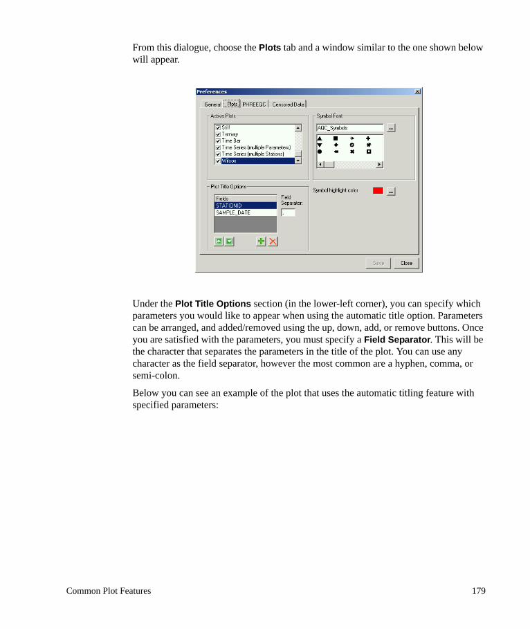
From this dialogue, choose the Plots tab and a window similar to the one shown below will appear.

Under the Plot Title Options section (in the lower-left corner), you can specify which parameters you would like to appear when using the automatic title option. Parameters can be arranged, and added/removed using the up, down, add, or remove buttons. Once you are satisfied with the parameters, you must specify a Field Separator. This will be the character that separates the parameters in the title of the plot. You can use any character as the field separator, however the most common are a hyphen, comma, or semi-colon.

Below you can see an example of the plot that uses the automatic titling feature with specified parameters:

Common Plot Features 179

NOTE: By default, all Pie, Radial, and Stiff plots will be titled automatically with the fields specified in the Preferences dialogue. To change the plot title after the plot has been created, simply type in a new plot title in the Plot Title field, and press [OK].

4.1.2 Symbols DialogueThe options in the Symbols dialogue allow you to edit the symbol appearance settings.

Show frameIn this frame you find the following options:

180 Chapter 4: Plots

• Show Symbol - show/hide symbols using this check-box• Display selected samples only - display only the samples selected from the

Samples List using this check-box (need to pre-select the samples)• Show precision - show/hide precision bars using this check-box (Precision

value must be entered for this particular parameter in the Sample Details window)

• Connecting lines - show/hide connecting lines using this check-box

Edit frame

Symbols

Click the button to open the Define Symbol or Line dialogue. In this dialogue, you can define the names and status of the symbol groups, the shape and color of the symbols, and the line-type and color of lines that appear in the plots (refer to the Define Symbol or Line section in Chapter 3 for a description of the symbol groups settings).

Labels

Click the button to open the Labels dialogue. In this dialogue you can specify the labels for each individual data point or for multiple data points at once. Select the text, font, and position for the label. For more detail see Labels dialogue section later in this chapter.

Scaled Symbol Size frame

Proportional to

This option allows you to scale the size of the plot symbols based on a user-defined parameter (TDS, pH, Cond, etc.). This allows you to represent an additional parameter on your plot. For example, in a scatter plot, you can display information on three parameters, instead of only two (X and Y). Once the parameter is selected, you can choose different units for this parameter.

Scaled from ... to ... Points

Defines the minimum and maximum radius of the scaled symbol size. The minimum symbol size will be plotted for the lower limit of the proportional parameter value, while the maximum symbol size will be plotted for the upper limit of the proportional parameter value. The minimum radius ensures that all symbols will be visible even if the proportional parameter value is zero.

Common Plot Features 181

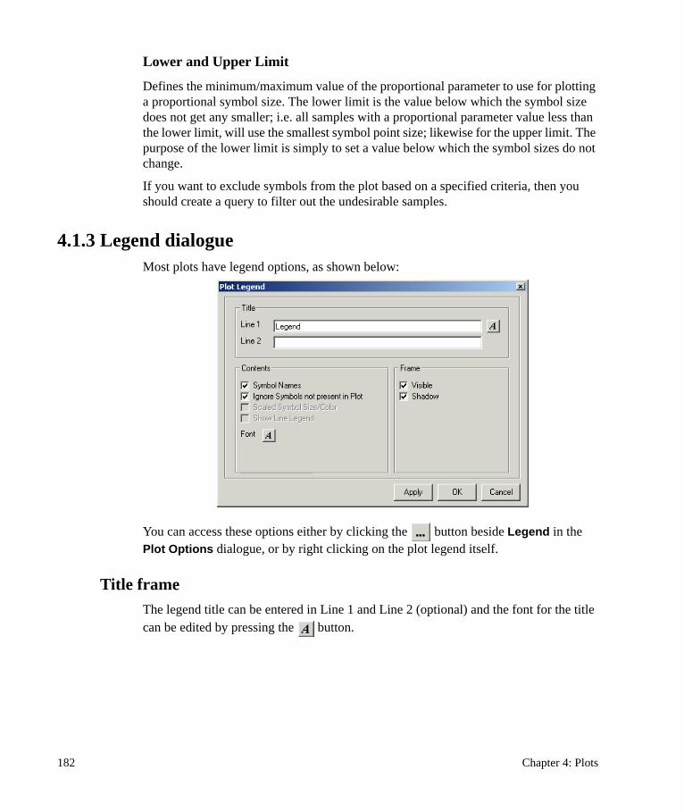
Lower and Upper Limit

Defines the minimum/maximum value of the proportional parameter to use for plotting a proportional symbol size. The lower limit is the value below which the symbol size does not get any smaller; i.e. all samples with a proportional parameter value less than the lower limit, will use the smallest symbol point size; likewise for the upper limit. The purpose of the lower limit is simply to set a value below which the symbol sizes do not change.

If you want to exclude symbols from the plot based on a specified criteria, then you should create a query to filter out the undesirable samples.

4.1.3 Legend dialogueMost plots have legend options, as shown below:

You can access these options either by clicking the button beside Legend in the Plot Options dialogue, or by right clicking on the plot legend itself.

Title frameThe legend title can be entered in Line 1 and Line 2 (optional) and the font for the title can be edited by pressing the button.

182 Chapter 4: Plots

Contents frame

Symbol Names

Show/hide symbol names using this check-box. When the legend is visible, the Symbol Names from the currently selected symbol group will be displayed on the plot. Use the font button below the options to edit the font of the symbol names as they appear in the legend.

Ignore symbols not present in plot

When this option is active, the plot will show only those symbols which are used in the current plot. For example if 10 symbols are active, but the current selection of samples only uses 2 of them, AquaChem will ignore those symbols that are not present in the plot and display just the 2 symbols in the legend.

Scaled Symbol Size/Color

This option is only active if you have symbol sizes plotted proportional to a parameter value, under the Symbols options. When this is activated, the legend will show a scale for the proportional symbol sizes.

Show Line Legend

Show/hide line legend using this check-box.

Frame frame

Visible

Show/hide box around the legend using this check-box.

Shadow

Show/hide the legend shadow effect using this check-box.

4.1.4 Line DialogueAquaChem allows you to put a calculated or user-defined regression line on your plot. For Time Series and Box and Whisker plots horizontal lines can also be added to represent line features such as Maximum Concentration Limit.

Common Plot Features 183

To create a new line click the in the upper right corner. The defined line follows the basic equation of y=mx+b and once a new line is created you need to specify these constants for the line. There are two ways of doing so: calculate a linear regression trend or enter user defined values.

Equation tab

Linear Regression frame

This frame allows you to calculate the linear regression constants based on various selections:

• All - calculates linear regression using all available stations• Selected - calculates linear regression using only selected series• Individual stations (names depend on the database) - calculates linear

regression based on one station

Once you’ve selected the data series, click the [Calculate] button to calculate the coefficients.

NOTE: The selection must include more than one point.

Formula frame

This frame allows you to enter custom values for the linear regression equation constants. If you used the Linear Regression frame to calculate values based on data

184 Chapter 4: Plots

points, these values will be displayed in this frame. If the Calculate feature was used, this frame will also display statistics of the calculations.

Adding a Horizontal Line (Time Series and Box and Whisker plots)To add a horizontal line to a Time Series or Box and Whisker plot to represent a feature such as a Maximum Concentration Limit line, simply create a new line in the Lines dialog and edit the line name as you would like it to appear in the plot legend. Then in the Formula frame, enter the Y-axis value where you would like the line to be positioned in the b field of the y=mx+b formula. The line can be included in the plot legend using the Legend dialogue (See section 4.1.3 for more information on the Legend dialogue).

Line Properties tabUse this tab to customize the line appearance on the plot.

Style frame

Set the Style, Color, and Width of the line.

X-Axis Limits frame

Set the maximum and minimum X-value for the generated line. If left and right are set to Auto, the line will span the entire plot.

Common Plot Features 185

4.1.5 Format dialogueThis dialogue is only available in plots on X-Y style plots with linear axes.

AxisThis combo box allows you to switch between the available axes.

Minimum/MaximumAllows you to customize the minimum and maximum axes values. AquaChem will determine a default minimum/maximum value based on all of the data plotted on the graph. If you enter a new value and you wish to return to automatic calculation, enter “A” in this field.

Labelled TicksDefines the interval value of the labelled ticks for the corresponding axis. AquaChem will determine a default value for the labelled ticks such that the plot will have 5 labelled ticks on the corresponding axis. If you enter a new value and you wish to return to automatic calculation, enter a value of “A” in this field.

Label AngleAllows you to specify the angle to the axis at which the labels appear. Tilted tick labels are recommended for long labels which run the risk of overlapping on smaller plots.

186 Chapter 4: Plots

Minor TicksDefines the number of minor ticks between each of the labelled ticks. The default value is 1. Only integer values are accepted.

FormatSets the numeric format for the labels on the axes (e.g. Auto, 0, 0.0, 0.00, 0.0E+00, etc.). Beside Format, click button in the combo box to select from the list of available numeric formats.

TitleDefines the title of the corresponding axis. If a title field is left empty, a default title equal to the internal name of the parameter will be selected by AquaChem. If you want to omit one or both axes titles, type a space in the text field(s). Use the button to change the font.

Log ScaleSome plots allow you to show the plot data using a log scale for either the X or Y axis, or both. This allows you to normalize the data set, if there is a significant range in the data.

4.1.6 Labels dialogueUse this dialogue to set up the label display properties.

Common Plot Features 187

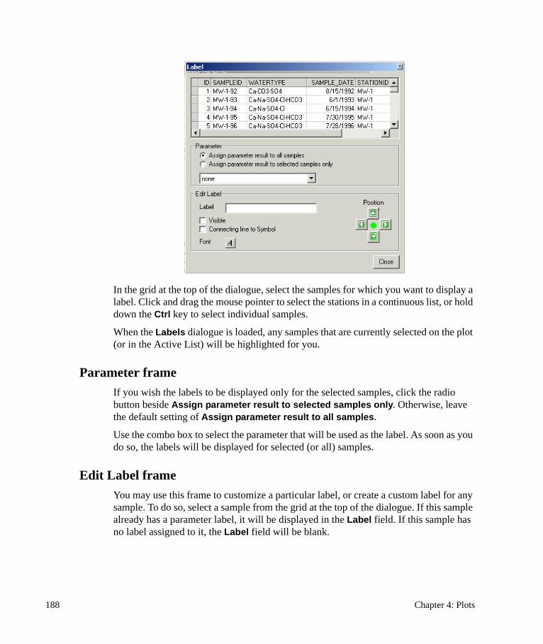
In the grid at the top of the dialogue, select the samples for which you want to display a label. Click and drag the mouse pointer to select the stations in a continuous list, or hold down the Ctrl key to select individual samples.

When the Labels dialogue is loaded, any samples that are currently selected on the plot (or in the Active List) will be highlighted for you.

Parameter frameIf you wish the labels to be displayed only for the selected samples, click the radio button beside Assign parameter result to selected samples only. Otherwise, leave the default setting of Assign parameter result to all samples.

Use the combo box to select the parameter that will be used as the label. As soon as you do so, the labels will be displayed for selected (or all) samples.

Edit Label frameYou may use this frame to customize a particular label, or create a custom label for any sample. To do so, select a sample from the grid at the top of the dialogue. If this sample already has a parameter label, it will be displayed in the Label field. If this sample has no label assigned to it, the Label field will be blank.

188 Chapter 4: Plots

Label

The label text is normally filled automatically from a database field. You may, however, edit this text or even enter all labels manually.

Visible

Use this check-box to display/hide the specified label for the selected sample(s).

Connecting line to Symbol

Use this check-box to display/hide a line connecting the symbol with the label. The connecting line is useful for densely placed symbols.

Font

Click the button to change the label font.

Position frameUse the arrow buttons to position the labels. The label position is updated as soon as you click the arrow button.

4.2 Plot ConfigurationsOnce you have created the desired plot, or combination of several plots, the Save Configuration option under the Plots menu is enabled. This allows you to save the current configuration of open plots and their settings, to your database.

The configuration includes axis settings, selected samples, symbol settings, etc.

When you select Save configuration, the dialogue shown on the right side will appear prompting you for a name for the Plot Configuration. Simply type in a name for the plot configuration.

Once you are finished, click [OK].

To recall a saved plot configuration in the future, use the Plots > Open Configuration option. Simply select the plot configuration you desire, then click [OK]. This will load

Plot Configurations 189

the plot(s) and their settings. When a plot configuration is loaded, the sample selection used for this plot will also be reset in the Active List window. Aquachem allows for multiple plots configurations to be open concurrently. To remove any unwanted or outdated plot configurations, simply select the respective item from the list, and press the button. Once you are finished, click [Close].

4.3 Save, Show, and Identify Plot Data

Show Sample DataIf this option is selected from the Plots menu, AquaChem will display a small dialogue with the data for the selected sample. Simply click on a sample point from the plot and the Info data dialogue will appear. Each time you click on a new sample point, the new data is loaded into dialogue. An example is shown below:

NOTE: You may need to re-arrange the positions of your windows in order to see the Sample Data dialogue.

190 Chapter 4: Plots

Identify Plot DataThe Identify option allows you to link the plotted data to the samples in the active list. This allows you to click on a point in the graph and view the corresponding sample in the active list. This is useful when you have a large number of samples displayed on one plot, and you want to identify outliers.

NOTE: You may specify the color in which the symbol is highlighted on the plot in the Plots tab of File>Preferences described in chapter 3.

There are three options available for selecting and identifying points on a plot: None, Selected Plot, and All Plots. The default mode to identify points is on All Plots; this means that all data points on all plots are linked to the database. These three options are described below:

None

If this option is selected, then no symbols will be highlighted on the plot when the samples are selected. The data points on the graphs are not linked to the database which means that samples are not identified. When you have several open graphs and a large database with many samples, it may be convenient to have no link between the graphs and the database in order to increase the speed of the various AquaChem operations.

Selected Plot

Only the data points in the active graph are linked to the database. The chosen point is activated (highlighted) and selected in the sample list. This mode is useful if you are working with a large data set and want to focus on just one graph.

All plots

The sampling point of the corresponding sample is activated on all plot windows and on the sample list. If you are working with several graphs, you can identify a sample in all plots as well as in the sample list by clicking near a point in any of the plots, or by clicking on a sample in the active list. The sample will become selected in the active list, and the corresponding data points will be highlighted in red in all the open plot windows.

4.4 Printing and Exporting PlotsOnce you are satisfied with your plot(s) and their design, you have four options for producing output:

• The plot can be saved as a Windows Metafile (.WMF) and printed from an external application, or inserted into a report;

Printing and Exporting Plots 191

• The plot can be copied to the Windows clipboard and pasted into another supported application (ex. a graphics program, MSPaint, or a word processor);

• The plot can be printed as is, or can be incorporated into a Printing Template which can include project information, company details, and your company logo.

4.4.1 Export as MetafileWhen you have any plot window open, you can save the plot as a Windows Metafile (graphics format) by selecting File from the main menu and then Export>Image. In the Save Plot As... dialogue that appears, enter a filename for this file and press [Save]. You can now open and manipulate this image using a graphics editor or insert this file into a report. When using this feature, each plot window must be saved individually as a metafile.

4.4.2 Copy Plot to ClipboardTo copy the selected plot to the windows clipboard, select Edit from the main menu and then Copy. If successful, a confirmation dialogue will appear.

The plot can then pasted directly into another application such as a word processor or a graphics editor.

192 Chapter 4: Plots

4.4.3 PrintingTo print one or more of the on-screen plots, select File from the main menu and then Print, while the plots window is active. Alternatively, you can click the icon from the AquaChem toolbar. A Print Options window will appear, as shown in the figure below:

The Print Options window has the following components:

Available Plots: Contains the list of plots that were open when Print option was selected, and thus are available for printing.

Plot Legends and Locations: Lists the X and Y location of the plot and the legend (if available).

Page Layout Options: Lists the available plot templates and options for customizing the report.

Print Preview Window: Provides a preview of the printed page.

To print one or more plots, you must select the desired plot(s) from the list of the Available Plots by placing a check mark in the box beside the appropriate plot. The

Page LayoutOptions

Print PreviewWindow

Plot Locations and Legends

Available Plots

Printing and Exporting Plots 193

selected plot(s) will appear in the Print Preview window and will be automatically sized and arranged to fit the page.

To select a plot, click once on the plot list to activate it, and then click once in the box beside the plot name. A check mark will be added to the box and this plot should appear in the Print Preview window. To load additional plot(s), simply click once with your mouse in the box beside the plot name(s).

To remove a plot from the Print Preview window, simply click once in the box to remove the check mark beside the appropriate plot.

Arranging the PlotsThe order of the plots can be easily modified using the arrow buttons below the list of plots. Selected plots can be moved up or down using these buttons. The position of each plot on the page can be modified in the Axis tab by entering a new X, Y origin; the size of each plot can be modified by entering a new X, Y length.

Clicking the [Auto] button will load the following dialogue:

In this dialogue edit the grid used to optimally position plots on the page.

If needed, click the [Refresh] button at the bottom of the screen to update the print preview.

Plots per page option allows you to spread the plots over several pages, as well as specify the number of plots to be arranged on each page.

Print Preview WindowThe Print Preview window provides a “What You See Is What You Get” (WYSIWYG) preview of the printed page. The page magnification value can be adjusted using the magnifying glass above the preview window. This will enlarge or shrink the appearance of the page preview on your screen. The page coordinates (cm) for the mouse pointer location are located in the upper left corner of this window.

194 Chapter 4: Plots

Selecting a Print TemplateThe Page Layout frame allows you to select from a list of pre-defined print templates which contain fields for descriptions of the plot(s), the project, client, and company information. In this frame there is also a Plots per page field. This allows the user to specify how many plots they would like to appear on each page when printing multiple plots.

Plot arrangement and page layouts can be saved as templates at anytime by selecting Save as Template from the File menu.

AquaChem includes the following pre-defined print templates:

• US Letter - Portrait• US Letter - Landscape• A4 - Portrait• A4 - Landscape

The default template selection is "None", meaning no print template is selected. If "None" is selected you have the option to enter a two line title at the top of the page plus a one line footer at the bottom of the page.

If the pre-defined print templates are not satisfactory for your needs, you can easily create your own customized print templates using the Template Designer option available by clicking the ‘...’ button beside the template selection list. For a detailed description of this component, please refer to the Template Designer section in chapter 3.

If you select one of the pre-defined print templates, a list of available descriptor fields will appear and the Print Preview window will be updated to reflect the layout of the selected template. Fill in the project specific plot description fields under the Page Layout options. Depending on the template, you may enter information for: CLIENT, PROJECT, PROJ #, DATE, DESCRIPTION.

An example of the Print Preview window with Fields is shown below:

Printing and Exporting Plots 195

Once you have entered the descriptive information for the plot, press the [Refresh] button to refresh the print preview.

When you are satisfied with the print layout, simply click the [Print] button in the lower left corner of the window, select File > Print from the main menu, or click the icon.

Alternatively, you may select Edit > Copy from the main menu, and the plot, along with the print template, can be copied to the clipboard, and pasted into an external application.

To return to the main AquaChem window, click the [Close] button.

4.5 Plot DetailsThis section describes each of the AquaChem plots and the options available for each plot.

196 Chapter 4: Plots

4.5.1 Box and WhiskerThe Box and Whisker plot displays a statistical summary of any measured database parameter(s). It is composed by a central box showing the spread of the bulk of the data (interquantile range) and the whiskers, showing the length of the tails.

The Box and Whisker plot can be displayed in three forms:

• Box and Whisker (Multiple Parameters)• Box and Whisker (Multiple Stations)• Box and Whisker (Time)

X-Axis frameIf you select Box and Whisker (Multiple Parameters) plot then select ONE station group in the Series field, and then specify one or more parameters under the Parameters list. If <all> is selected, then all samples from the active list will be used. The options for this plot are shown below.

An example of the Box and Whisker (Multiple Parameters) plot is shown in the figure below.

Plot Details 197

If you select Box and Whisker (Multiple Stations) plot then you will see the Parameters and Series fields become reversed. You need to specify ONE parameter beside the Parameter field and then enter one or more station in the Series field. The options for this plot are shown below.

An example of the Box and Whisker (Multiple Stations) plot is show in the figure below:

198 Chapter 4: Plots

If you select Box and Whisker (Time), the analysis will be performed on all samples in the Sample List. AquaChem can aggregate the samples by month, season or year. Note that the season and month group may include samples from different years and are particularly useful for seasonal analysis.

An example of the Box and Whisker (Time) plot is shown in the figure below:

Plot Details 199

Select the statistics to be displayed as whiskers using the Whiskers combo box.

Whereas the extent of the central box is standardized (25%, 75% quantiles), the extent of the whiskers is not. The whiskers combo box, therefore, lets you choose, which position of the tails of the underlying population should be used to displayed by the whiskers: Min/Max extent, 5/95% or 10/90% quantiles. If the whiskers are defined as a quantile value, then the minimum and maximum values can be added as a further information to the plot and will be shown as points above and below the whiskers.

Click the button beside Format to produce the Axis dialogue. Use this dialogue to customize the x-axis appearance.

Y-Axis frameUnless all parameters you wish to plot are unitless, this frame allows you to select the display unit using the Unit combo box.

Click the button beside Format to load the Axis dialogue. Use this dialogue to customize the y-axis appearance and apply log transformation if necessary.

Plot frame

Click the button beside Title to load the Title dialogue.

Check the box beside Legend to enable the plot legend. Click the button to load the Legend dialogue and customize the display options.

Check the box beside Show Grid to display the gridlines.

Click the button beside Lines to load the Lines dialogue. In this plot the Line option may be used to draw a horizontal line representing the standard for the or one of

200 Chapter 4: Plots

the plotted parameters. This can be done manually by creating a line y=mx+q where m=0 and q equal to the standard for this parameter.

If the standard value is defined in the active water standard, then clicking on the [Standard] button will automatically create this line for you.

Fill Color/Pattern

Click the button beside Color to select the fill color for the box plot.

Click the button beside Pattern to choose the display pattern for the box plot.

For more details on this plot, please refer to the article: Tukey J.W., 1977: Exploratory Data Analysis, Addison-Wesley, Reading, Massachusetts, USA. 1977, pp. 39-43.

4.5.2 Depth ProfileThe Depth Profile plot displays the change in a parameter value as sample depth changes. An example of a Depth Profile plot and the corresponding Depth Profile Plot Settings dialogue is shown in the figure below.

The Depth Profile plot is similar to a borehole log. The plot displays the change of a measured parameter over a measured sampling depth. In order to create this plot, you must have an entry for the parameter Sample_Depth for one or more samples in your database. You may then plot the Depth (on the Y-Axis) against any measured parameter (on the X-Axis).

Plot Details 201

X-Axis and Y-Axis frames

Click the button beside the Parameter field in the X-Axis frame to select the parameter to be plotted on the x-axis. The parameter for the y-axis frame is Depth and cannot be changed.

Select the units for the x-axis parameter using the Unit combo box in the X-Axis frame. The unit for the y-axis depends on the Depth parameter unit in the database and cannot be changed in this dialogue.

Click the button beside Format in the X-Axis and Y-Axis frames to access their respective settings dialogues.

Plot frame

Click the button beside Title, Symbols, Lines, Legend, and Labels to access their respective settings dialogues. The Legend and Labels features must be activated (the box beside them must be checked) before their dialogues can be loaded.

Check the box beside Show Grid to display the gridlines.

4.5.3 Detection summaryThe Detection Summary plot is used to visualize the relative proportions of samples above the specified water quality standards. The plot shows a summary bar for every parameter specifying the percentage of values where the contaminant has not been detected, where it has been detected but is below the water quality standard and the percentage of samples exceeding the water quality standard. Below is the Detection Summary plot options and the corresponding plot:

202 Chapter 4: Plots

On the left side of each detection summary bar you can see the number of samples that have a value for the parameter that this bar represents. The parameter name is listed on the right side of each detection summary bar. The X-axis lists cumulative percent values from 0 to 100. You can calculate the number of samples that exceed a particular standard (or are non-detects) by multiplying the percent “length” of the particular colored segment by the number of samples used to produce a particular detection summary bar.

NOTE: Parameter values that contain “<“ symbol will be included in “below MDL” category.

Axis frame

Click the button beside the X-axis Format and Y-axis Format to load their respective options dialogues.

Parameters frameUse this frame to select the parameters for which you wish to produce the detection summaries. Use the button to add parameters (select from the presented list), the

button to delete parameters, and and buttons to change the order in which they appear on the plot.

Plot frame

Click the button beside Title and Legend to access their respective dialogues. The Legend feature must be activated (checked) before the options dialogue can be loaded.

Use the check box beside Show Grid to show/hide the gridlines.

Use the check box beside Show number of samples to show/hide the number of samples displayed to the left of the detection summary plot.

Fill colors frame

Use this frame to customize the display colors for detection summary plot. Use the button to access the color selection dialogue.

4.5.4 Durov PlotThe trilinear Durov plot is based on the percentage of major ion milliequivalents. The Cations and Anions values are plotted on two separate triangular plots and the data

Plot Details 203

points are projected onto a square grid at the base of each triangle. The Durov plot is an alternative to the Piper plot which is described later in this chapter.

Since the data points are projected along the base of the triangle, which lies perpendicular to the third axis in each triangle, information about the concentration of the vertex element (the third element) is lost in the square grid. Changing the orientation of parameters in both triangles may improve your ability to detect distinct groups.

An example of Durov plot and the corresponding Durov Plot Options dialogue is shown in the figure below.

Cations and Anions framesThe Cations specify the parameters of the left triangle. Default settings are the major cations Na, Ca, and Mg, however any other parameter can be selected (e.g. gas composition, trace elements etc.). The Anions generally specify the parameters for the upper triangle. Default settings are the major anions Cl, SO4, and HCO3, however any other parameters can be selected. Note that measured Alkalinity is a valid anion parameter, provided the respective parameter is known by the system as being the Alkalinity. This may be done on the File>Database>Alias tab by assigning the respective parameter to the Measured Alkalinity. If using the alkalinity in the anion triangle, change the respective displayed label field to HCO3 + CO3.

Data from poorly concentrated parameters can be multiplied by a common factor to prevent data point accumulation on a base line when plotting parameters with very different concentrations. Type the multiplication Factor in the field beside the parameter.

204 Chapter 4: Plots

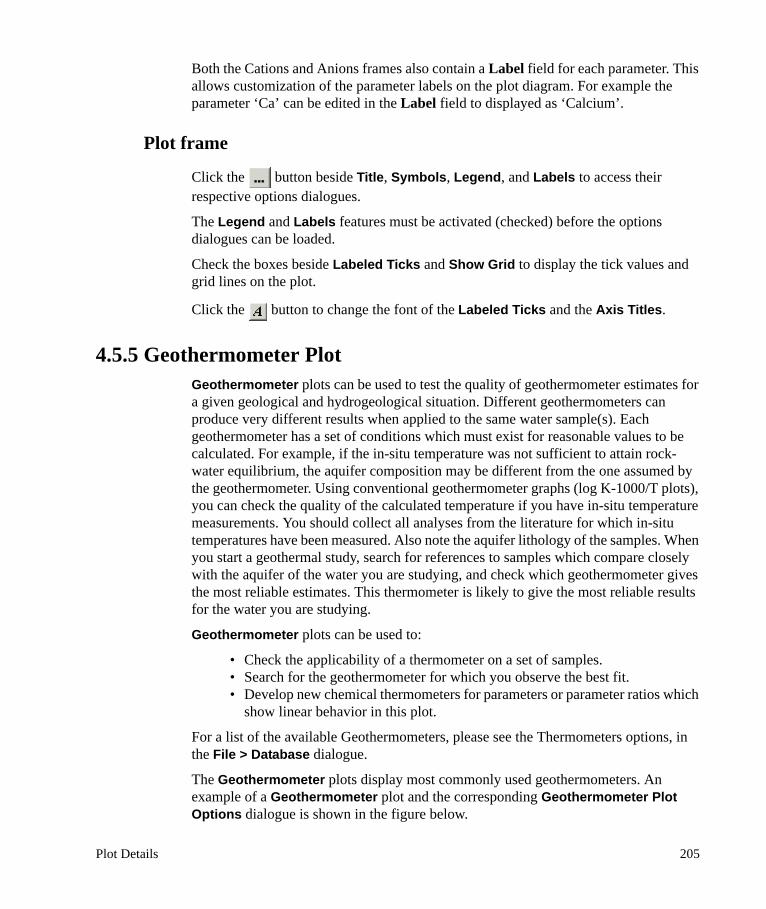
Both the Cations and Anions frames also contain a Label field for each parameter. This allows customization of the parameter labels on the plot diagram. For example the parameter ‘Ca’ can be edited in the Label field to displayed as ‘Calcium’.

Plot frame

Click the button beside Title, Symbols, Legend, and Labels to access their respective options dialogues.

The Legend and Labels features must be activated (checked) before the options dialogues can be loaded.

Check the boxes beside Labeled Ticks and Show Grid to display the tick values and grid lines on the plot.

Click the button to change the font of the Labeled Ticks and the Axis Titles.

4.5.5 Geothermometer PlotGeothermometer plots can be used to test the quality of geothermometer estimates for a given geological and hydrogeological situation. Different geothermometers can produce very different results when applied to the same water sample(s). Each geothermometer has a set of conditions which must exist for reasonable values to be calculated. For example, if the in-situ temperature was not sufficient to attain rock-water equilibrium, the aquifer composition may be different from the one assumed by the geothermometer. Using conventional geothermometer graphs (log K-1000/T plots), you can check the quality of the calculated temperature if you have in-situ temperature measurements. You should collect all analyses from the literature for which in-situ temperatures have been measured. Also note the aquifer lithology of the samples. When you start a geothermal study, search for references to samples which compare closely with the aquifer of the water you are studying, and check which geothermometer gives the most reliable estimates. This thermometer is likely to give the most reliable results for the water you are studying.

Geothermometer plots can be used to:

• Check the applicability of a thermometer on a set of samples.• Search for the geothermometer for which you observe the best fit.• Develop new chemical thermometers for parameters or parameter ratios which

show linear behavior in this plot.

For a list of the available Geothermometers, please see the Thermometers options, in the File > Database dialogue.

The Geothermometer plots display most commonly used geothermometers. An example of a Geothermometer plot and the corresponding Geothermometer Plot Options dialogue is shown in the figure below.

Plot Details 205

The following section describes some of the features and options of the Geothermometer Plot that are not covered in the Common Plot Features section.

Geothermometers are generally expressed by the formula:

where, x is the SiO2 concentration or Na/K, etc., log (x) values plot on a straight line as a function of 1000/T. The coefficients a and b are obtained empirically from deep borehole data with in situ temperature measurements.

Axis frame

Click the button beside X-axis format and Y-axis format to access their respective options dialogues.

Plot frame

Click the button beside Title, Legend, Symbols, Labels, and Lines to access their respective options dialogues. The Legend and Labels features must be activated (checked) before the dialogues can be loaded.

Use the Show Grid check box to show/hide the plot grid lines.

Thermometer ListSelect (highlight) the thermometer to be used for the plot.

t K( ) 1000 ab x( )log+-------------------------=

206 Chapter 4: Plots

For more details on Geothermometers, please refer to the following article:

Kharaka et al. 1989.

4.5.6 Giggenbach TriangleThe Giggenbach triangle provides a visual aid to determine the water-rock equilibrium. An example of the Giggenbach Triangle plot and the corresponding Giggenbach Triangle Options dialogue is shown in the figure below.

The Giggenbach Triangle (K-Mg-Na Triangle) representation allows you to verify the extent to which water-rock equilibrium has been attained.

The triangle is comprised of three zones:

• Immature waters (at the base);• Partially equilibrated waters (in the middle); and• Fully equilibrated waters (along the curve).

Depending on where the composition of a given sample lies within this triangle, you can estimate the extent of rock-water equilibrium. For mature waters falling near the upper curve, you can estimate the temperature as well.

Giggenbach Triangle frameEnter the division factors for Na and K in the text fields provided. The default values for the plot are Na/1000 and K/100.

Use the Labeled Ticks check box to show/hide the tick values.

Click the button to modify font for the tick values and parameter labels.

Plot Details 207

Plot frame

Click the button beside Title, Symbols, Legend, and Labels to access their respective options dialogues. The Legend and Labels features must be activated (checked) before the options dialogues can be loaded.

Use the Show Grid check box to show/hide the plot grid lines.

For more details on the Giggenbach Triangle, please refer to the following article:

Giggenbach, W.F., 1988. Geothermal solute equilibria. Derivation of Na-K-Mg-Ca geoindicators. Geochim Cosmochim. Acta, 52: pp. 2749-2765.

4.5.7 HistogramTwo of the oldest methods for summarizing data distributions are the frequency and histogram plots. Both the histogram and the frequency plot use the same basic principles to display the data: dividing the data range into units, counting the number of points within the units and displaying the data as the height within a bar graph. An example of a Histogram plot and the corresponding Histogram Plot Options dialogue is shown in the figure below.

You can easily identify a single sample in a multi-sample histogram plot by clicking on the sample in the Active Samples List. A red triangle will be displayed on the histogram, indicating the range interval of the selected sample (this is a unique feature of AquaChem and is not normally found in other histogram plotting software). Clicking on a bar on the graph will select all the samples in the Active List which are included within the interval range defined by the histogram bar you selected.

208 Chapter 4: Plots

X-Axis frame

Use the button beside Parameter to select parameter to be plotted on the histogram. This field can also handle parameter ratios, sums, or differences (e.g. Na/Cl, Ca+Mg, Cl-SO4). Enter these parameter combinations into the parameter field manually. Unless the parameter you’ve chosen is unitless (e.g. pH), the Unit combo box will allow you to select the units for the parameter.

The Classes field defines the number of data classes (or intervals) into which the range of parameter values will be subdivided. Each data class will be represented by a single bar on the histogram. Type the number of classes (bars in the histogram) in the provided field.

Click the button beside Format to load the corresponding axis options dialogue.

Y-Axis frameThe number of samples within each data class is referred to as the frequency of occurrences. This can be expressed as either a percentage of the total number of samples (Percents), or as the number of samples within each data class (Number of hits). Select the desired option.

Click the button beside Format to load the corresponding axis options dialogue.

Plot frame

Click the button beside Title to load the title options dialogue. Check the box beside Show Grid to display the grid lines.

Fill Color and Pattern frame

The color and pattern of the bars in the graph can be modified using the options beside Color and Pattern. Simply press the button to access the various options.

4.5.8 Ludwig-Langelier PlotThe Ludwig-Langelier plot allows you to quickly see patterns and correlations between the major cations and anions for multiple samples. An example of the Ludwig-Langelier plot and the corresponding Ludwig-Langelier Plot Options dialogue is shown in the figure below.

Plot Details 209

The Ludwig-Langelier square plot is similar to the projection areas of the Piper and Durov plots. By convention, the sums of selected cations are plotted on the X-Axis and the sums of selected anions are plotted on the Y-Axis. Each axis ranges from 0 to 50 meq%. Sample points are calculated as follows:

%

%

Suitable groupings of cations and anions are selected and plotted as percentages. Generally, this type of graph is used to plot %Na+%K against %HCO3+%SO4. In this plot, %Ca+%Mg and %Cl are also fixed:

%Ca+%Mg =50 - (%Na+%K)

%Cl =50 - (%HCO3 +%SO4)

Sanions Cl SO4 HCO3+ +=

Scations Ca Mg Na K+ + +=

Na 50 NaScat-----------=

Cl 50 ClSan----------=

210 Chapter 4: Plots

All major elements can be displayed in one plot with the Ludwig-Langelier plot, however like the Piper and Durov plots, the plot displays relative ratios rather than absolute concentrations.

X-Axis and Y-Axis frames

Click the button beside the Parameter field to select the first of the parameters. The remaining parameters must be added manually.

Click the button beside Format to load the axis options dialogue for the corresponding axis.

Plot frame

Click the button beside Title, Symbols, Legend, and Labels to load the corresponding dialogue. The Legend and Labels features must be activated (checked) before their options dialogues can be accessed.

Use the Show Grid check box to show/hide the plot grid lines.

4.5.9 Map PlotThe Map plot reads the X, Y coordinates for the station location, and displays this on a blank grid or on a site map of your site. The Map plot can import and overlay an AutoCAD (.DXF) file, an ESRI shape (.SHP) file, or a common graphics (.BMP, .JPG, and .GIF) file as a basemap of the site or study region defining the major physical and geographical boundaries and geological characteristics.

The Map plots can be used to simply display the station locations throughout the study region, or to interpret spatial trends in the physical or chemical characteristics of each sample using proportional symbol sizes, or by plotting Pie, Radial or Stiff graphs at each sample location. The Radial and Stiff symbols may be exported to ESRI polygon shapefile format.

NOTE: You must have at least one station in your database with X and Y co-ordinates in order to create a Map plot.

When you choose a Map as the plot type, the following Map Plot Options dialogue will appear:

Plot Details 211

Axis tab

Axes frame

Click the button beside X-axis format and Y-axis format to access the corresponding dialogues.

Plot frame

Click the button beside Title, Legend, and Label to access their respective options dialogues. The Legend and Labels features must be activated (checked) before the options dialogue can be loaded.

Use the Frame and Show Grid check boxes to show/hide the frame around the map and the plot grid lines.

Base Map frame

AquaChem allows you to load multiple maps in various file formats as the base map for the plot. You can load any of the following types of files: .DXF, .SHP, .BMP, .JPG, and .GIF. If the format of the file you wish to load is not listed above, use a graphics editor to convert it into one of the listed formats.

To add a basemap to your plot click the button. In the Base Map File dialogue that is loaded select the appropriate file type and navigate to the desired file. Click [Open] to load the map and the file name will appear in the Base Map frame as shown below.

212 Chapter 4: Plots

If you loaded a .DXF or a .SHP file, the min X/max X and min Y/max Y coordinates are entered automatically. For the ESRI shape files you will also have the options of changing the line width and color.

For shape files, additional options will appear allowing you to specify line width and color.

NOTE: The images must be georeferenced in feet or meters (the units have to be the same as the station X-Y coordinates). AquaChem does not support Lat/Long coordinate system.

If you load a common graphics file (.BMP, .JPG, or .GIF), the program automatically assigns one meter (or foot) per pixel in the picture. This image has to be manually georeferenced.

Simply enter the new coordinates for 2 corner points of the map.

If you wish to change the source file for the currently highlighted map, click the button to load a new file.

You may load multiple maps into your map plot. Use the and buttons to change the order in which they appear in the plot and the check box beside the name to show/hide the respective map image.

Symbols tabThe Symbols tab in the Map Plot Options dialogue allows you to choose a symbol to represent the samples on the map plot

Plot Details 213

Symbol frame

There are six symbol types to choose from:

• Plain Symbol• Proportional Size• Proportional Greyscale• Pie Chart• Radial Diagram• Stiff Diagram

Depending on the type of symbol you choose, the lower preview frame will show different plot and the third tab (available only for Pie Chart, Radial Diagram, and Stiff Diagram) will present different options to customize the chart.

Plain Symbol

The Plain Symbol type will plot the symbol shapes, sizes and colors as they are defined for each sample group. Press the button beside the field to access the Define Symbol or Line dialogue for viewing or modifying the symbol settings for the database.

Proportional Size Symbols

The Proportional Size symbol type will plot the defined symbols at each sample location with a symbol size determined by the value of a selected parameter. By default, AquaChem selects Na as the proportional parameter. The sample values for the proportional parameter will be used to determine the radius of the symbol at each

214 Chapter 4: Plots

sample location (e.g.samples containing higher values of the proportional parameter will have a larger symbol radius).

To change the proportional parameter, type in the internal name of the desired parameter in the Parameter field, or click the button and select another parameter from the list.

The Radius field is used to set the minimum and maximum symbol radius (in points). The minimum symbol radius corresponds to the Lower Limit value of the proportional parameter, while the maximum radius corresponds to the Upper Limit value. Use a non-zero minimum radius to plot symbols at sample locations containing very low values of the proportional parameter. The symbol radius at each sample location is determined using a linear interpolation between the Upper Limit value and the Lower Limit value.

Proportional Greyscale

This symbol type will display a Greyscale symbol at each sample location, with the scale determined by the value of a selected parameter. The sample values for the proportional parameter will be used to determine the greyscale color of the symbol at each sample location (e.g. samples containing higher values of the proportional parameter will have a darker greyscale). To change the proportional parameter, simply type in the Internal name of the desired parameter in the Parameter field, or click the

button and select another parameter from the parameters list. Sample with values less than the Lower Limit value are assigned a white symbol color, while points with values equal to or greater than the Upper Limit value are assigned a black color fill.

Sample Aggregation

If you wish to display only one sample for every station in your project, this frame allows you to select the criteria according to which this sample will be chosen:

Select the appropriate criterion. Select None if you wish all samples to be considered.

The following aggregation options are available:

• Selected Samples only - only the samples currently selected in the Samples List will be displayed

Plot Details 215

• Representative samples only - only samples that are marked as Representative in the Samples List will be displayed

• Most recent sample per station - one sample with the latest date will be displayed for each station

• Oldest sample per station - one sample with the earliest date will be displayed for each station

• Smallest value - presents an option to choose a parameter based on the value of which one sample (with the smallest value) will be displayed

• Highest value - presents an option to choose a parameter based on the value of which one sample (with the largest value) will be displayed

• Closest to average - presents an option to choose a parameter based on the value of which one sample (with the value closest to the station mean) will be displayed

Preview frame

This frame is available only for Pie, Radial and Stiff Diagrams. It presents a generalized view of the chosen plot and the [Edit] button. Clicking on this button will move you to the third tab which, depending on the plot type you chose, will be one of the described below.

Pie Chart tabThis symbol type will display a Pie chart of the selected parameters at each sample location.

216 Chapter 4: Plots

Parameters list

Click the button to add parameters to the pie chart and the to delete them. Use

the and buttons to change the order of the parameters.

Fill Style frameUse the buttons beside Fill Color and Fill Pattern to specify these features.

Use the Units combo box to select the units for the parameters that require them.

Type in the symbol size in centimeters in the Symbol Size text box.

Inside Circle frame

If you wish, you can display one parameter as an inside circle of the pie plot. Click the button to select the parameter from the list and enter the Maximum Value for the

parameter. The samples containing a Proportional parameter concentration equal or greater than the Maximum Value will have an inside circle with the maximum radius. The inside circles for samples with Proportional parameter concentrations less than the Maximum Value will have a proportionally smaller radius.

An example of a Map Plot with Pie charts as sample symbols is shown below.

Radial Diagram tabThis plot will display a Radial Diagram of the selected parameters at each sample location.

Plot Details 217

Parameters list

Click the button to add parameters to the radial diagram and the to delete them.

Use the and buttons to change the order of the parameters.

Axes frame

Set the Minimum and Maximum values for the axes. AquaChem will select the optimum values, however they may not be what you want.

Select the units for the parameters using the Units combo box.

Set the Symbol Size. This value is the radius of the symbols as they appear on the printed output. Depending on your monitor’s resolution they may seem different on the screen.

You may log-transform your data using the Log scale check box.

Fill Style frame

Use the buttons beside Fill Color and Fill Pattern to specify these features.

Use the Units combo box to select the units for the parameters that require them.

Type in the symbol size in centimeters in the Symbol Size text box.

218 Chapter 4: Plots

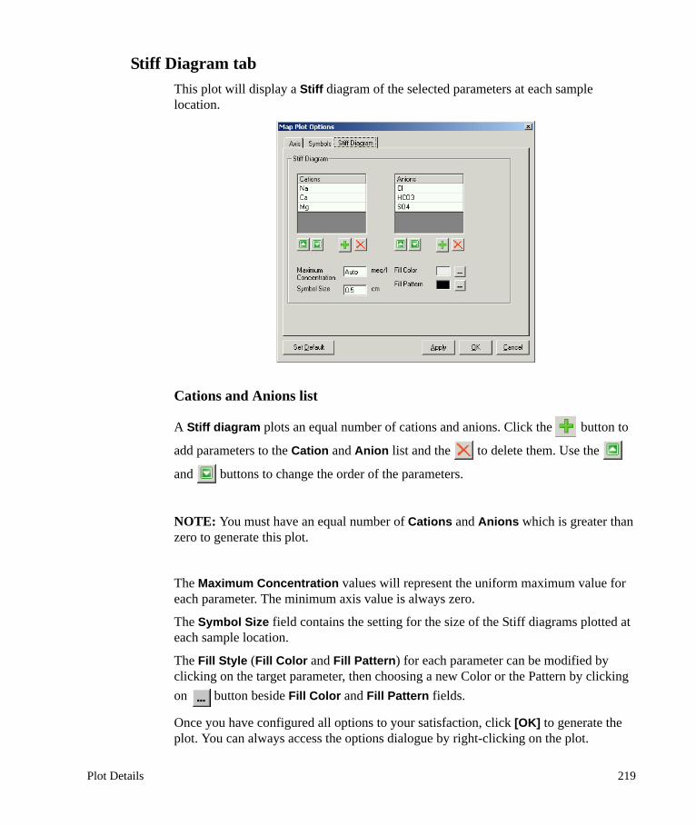
Stiff Diagram tabThis plot will display a Stiff diagram of the selected parameters at each sample location.

Cations and Anions list

A Stiff diagram plots an equal number of cations and anions. Click the button to

add parameters to the Cation and Anion list and the to delete them. Use the

and buttons to change the order of the parameters.

NOTE: You must have an equal number of Cations and Anions which is greater than zero to generate this plot.

The Maximum Concentration values will represent the uniform maximum value for each parameter. The minimum axis value is always zero.

The Symbol Size field contains the setting for the size of the Stiff diagrams plotted at each sample location.

The Fill Style (Fill Color and Fill Pattern) for each parameter can be modified by clicking on the target parameter, then choosing a new Color or the Pattern by clicking on button beside Fill Color and Fill Pattern fields.

Once you have configured all options to your satisfaction, click [OK] to generate the plot. You can always access the options dialogue by right-clicking on the plot.

Plot Details 219

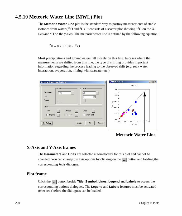
4.5.10 Meteoric Water Line (MWL) PlotThe Meteoric Water Line plot is the standard way to portray measurements of stable isotopes from water (18O and 2H). It consists of a scatter plot showing 18O on the X-axis and 2H on the y-axis. The meteoric water line is defined by the following equation:

2H = 8.2 + 10.8 x 18O

Most precipitations and groundwaters fall closely on this line. In cases where the measurements are shifted from this line, the type of shifting provides important information regarding the process leading to the observed shift (e.g. rock water interaction, evaporation, mixing with seawater etc.).

X-Axis and Y-Axis framesThe Parameters and Units are selected automatically for this plot and cannot be changed. You can change the axis options by clicking on the button and loading the corresponding Axis dialogue.

Plot frame

Click the button beside Title, Symbol, Lines, Legend and Labels to access the corresponding options dialogues. The Legend and Labels features must be activated (checked) before the dialogues can be loaded.

Meteoric Water Line

220 Chapter 4: Plots

Use the Show Grid check box to show/hide the plot grid lines.

NOTE: this plot is only active if your database contains the parameters 18O and 2H and if these parameters are mapped in the Alias section.

4.5.11 Pie PlotThe Pie plot is a simple way of showing parameter portions in a sample. An example of the Pie plot and the corresponding Pie Plot Options dialogue is shown in the figure below.

When you choose the Pie chart, a plot will be created for every sample selected in the active sample list. Before using this option, ensure that only the samples you want to plot are selected.

You must create a generic pie plot for every sample before you can customize it for each individual one. To do so, in the initial options dialogue set up the general options for the Pie plot - parameters to be plotted, their color and pattern, etc. Once this is done, click [OK]. A pie plot will be created for every selected sample. Right click on any of the pie plots to launch the Pie Plot Options dialogue and use it to customize the plots for each sample.

SampleAt the top of the Pie Plot Options dialogue, there is a Sample field which identifies the active sample(s) associated with the plot options dialogue. If you have created

Plot Details 221

several Pie charts, you can use the Sample field to select and modify the settings for each pie plot individually, or several at once as shown below.

To make changes to multiple plots simultaneously, simply select all of the samples you wish to edit in the list above (using your mouse), make the required plot changes then click [Apply]. This is useful for normalizing the axes scales, units, and general formats for each of the open Pie charts. If just one sample is highlighted and selected in this dialogue, then the changes will only be applied to this plotted sample.

Parameters frame

Parameters list

The Parameters list contains the parameters that will be plotted on the Pie chart. Existing parameters can be changed by selecting the parameter, and then typing in the name of the new parameter in the same field. New parameters can be added to the list by clicking the button and selecting a parameter from the available list. The new parameter will then be added to the bottom of the list. Parameters can be removed from the list by selecting the parameter and clicking the button. The order of the

parameters in the list can be adjusted using the and buttons.

Fill Style frame

The Fill Style allows you to edit the appearance of each pie slice in the plot. Select a parameter from the Parameters list, then select the Pattern and the Color you wish to assign to that slice of the pie chart. Repeat for the other parameters in the list.

Unit frame

Allows you to set display unit. The typical unit is meq/l which places cations in the upper part of the plot and anions in the lower part or vice versa, and permits a visual control of the electroneutrality.

222 Chapter 4: Plots

Inside Circle frame

The Inside Circle is used to represent the concentration of a single parameter (or combination of parameters) that is not included in the Pie chart parameters. You can specify any chemical or physical parameter that reveals the most comprehensive information about the sample. For example, you may want to display the CO2 or SiO2 concentration for the selected sample. Type a valid parameter in the Proportional to field to create an inside circle on your pie chart. Type a Maximum Value in the next field below (or use the default value). If several pie charts are created, it is recommended that you choose 3 to 4 times the average value of the inside parameter as the maximum value. All values that are greater than or equal to the maximum value are displayed with the maximum diameter. The inside circle will have a radius between zero and the specified maximum radius (R).

• R= Maximum radius for the internal circle• Value = value for this sample for the selected parameter.• Maximum Value: Maximum value above which, the full internal circle is

drawn.• Inside Radius = (Value / Maximum Value) * (pR/2)

Unless the parameter you have selected is unitless, you must also specify the units using the Units combo box.

Plot frame

Click the button beside Title and Legend to load the corresponding options dialogues. Pie plots are titled automatically according to the settings in File>Preferences>Plots. The Legend feature must be activated (checked) before the settings dialogue can be accessed.

Slice labels frame

The Slice Label options will apply a label to each slice of the pie chart. You can choose from Parameter Name, Concentration, Percentages, or None for no label.

4.5.12 Piper PlotThe Piper plot is useful for showing multiple samples and trends in major ions. An example of the Piper plot and the corresponding Piper Plot Options dialogue is shown in the figure below.

Plot Details 223

In the Piper plot, major ions are plotted as cation and anion percentages of milliequivalents in two base triangles. The total cations in meq/l, and the total anions in meq/l, are set equal to 100%. The data points in the two triangles are then projected onto the diamond grid. The projection reveals certain useful properties of the total ion relationships. Every sample is represented by three data points; one in each triangle and one in the projection diamond grid.

If your database stores carbonate species concentration as alkalinity, you may use the parameter alkalinity instead of HCO3 + CO3. Then change the label field to HCO3 + CO3.

The Piper plot allows comparisons of 6 parameters between a large number of samples. Like all trilinear plots, it does not portray absolute ion concentrations. The main purpose of Piper plots is to show clustering of samples.

Cations and Anions framesThe default parameter settings include the major cations (Na, Ca, and Mg) against the major anions (Cl, SO4 and HCO3); however, any other parameters, or combination of parameters, can be easily selected (e.g. gas composition, trace elements etc.)

The parameters can be modified by typing the Internal name of the parameters in the appropriate fields, or pressing the button and selecting another parameter from the available list. You may also multiply or divide the parameter concentrations by a factor if you need to compare elements which are systematically very different in concentration (e.g. comparing a trace element together with major ions). Finally, you may also enter parameter operators and functions (e.g. Na+K or Na/Cl); to do this, simply enter Na+K (for example) in the parameter field manually, and press [Apply]. However multiple parameters (e.g. Na, Cl) are not accepted.

224 Chapter 4: Plots

Both the Cations and Anions frames also contain a Label field for each parameter. This allows customization of the parameter labels on the plot diagram. For example the parameter ‘Ca’ can be edited in the Label field to displayed as ‘Calcium’.

Plot frame

Use the link buttons in this frame to modify the options for the Title, Legend, Symbol, Labels, and Format.

4.5.13 Probability plotProbability plots involve plotting quantiles of a data against the quantiles of the normal distribution. They are particularly useful for spotting irregularities within the data when compared to a specific distributional model, like the Normal. It is easy to determine whether departures from Normality are occurring more or less in the middle ranges of the data or in the extreme tails. Probability plots can also indicate the presence of possible outlier values or a different population that do not follow the basic pattern of the data and can show the presence of significant positive or negative skewness. The log scale transformation on the y-axis may be used to test whether a dataset that shows non normal behavior is simply normally distributed.

X-Axis frame

Use the button beside Format to set the Y-axis options.

Y-Axis frame

Select the parameter to plot by clicking the button and choosing from the parameter list. If the chosen parameter has units, a Units combo box will be presented in which you can select the desired units.

Use the button beside Format to set the X-axis options.

Plot frame

Use the button beside Title, Legend, Symbol and Lines to set their options. Check the box beside Show Grid to display the gridlines on the plot. Creating correlation lines may be useful to visually test whether data is distributed on a straight line, indicating a normal distribution of the underlying data set. if the y-axis is set to log scale, then the alignment of the data on a line indicates lognormal distribution.

Plot Details 225

4.5.14 Quantile PlotThe Quantile chart plots the ranked data from lowest to highest on the background of lines that denote 25% Quartile, Median, and 75% Quartile.

X-Axis frame

Use the button beside Format to set the Y-axis options.

Y-Axis frame

Select the parameter to plot by clicking the button and choosing from the parameter list. If the chosen parameter has units, a Units combo box will be presented in which you can select the desired units.

226 Chapter 4: Plots

Use the button beside Format to set the X-axis options.

Plot frame

Use the button beside Title, Legend, and Symbol to set their options. Check the box beside Show Grid to display the gridlines on the plot.

4.5.15 Radial PlotThe Radial plot is used to compare multiple parameter values for a single sample and to compare the ratios of these values for many different samples. An example of the Radial plot and the corresponding Radial Plot Options dialogue is shown in the figure below.

Radial plots can be used to evaluate the change in water quality at a single location over a period of time, or they can be used to evaluate the change in water quality as the water passes through different geologic formations or different subsurface conditions. A plot will be created for every selected sample in the Active Samples List. Before using this option, ensure that only the samples you want to plot are selected.

SampleThe Sample field identifies the active sample(s) associated with the plot options dialogue. If you have several Radial plots open, you can use the Sample field to select and modify the settings for each one.

Plot Details 227

To make changes to multiple plots simultaneously, simply select all of the samples in the list above (using your mouse), make the required plot changes, then click [Apply]. This is useful for normalizing the axes scales, units, and general formats for each of the open Radial plots. The changes apply to most of the graph settings that affect the appearance of the Radial plot, with the exception of the plot title. If just one sample is highlighted and selected in this dialogue, then the plot options changes will only be applied to this plotted sample.

Parameters frameThe Parameters list contains the parameters that will be plotted on the Radial plot. A Radial plot requires a minimum of three parameters. Existing parameters can be changed by selecting the parameter, and then typing in the name of the new parameter in the same field. New parameters can be added to the list by clicking the button and selecting a parameter from the available list. The new parameter will then be added to the bottom of the list. Parameters can be removed from the list by selecting the parameter and clicking the button. The order of the parameters in the list can be

modified by selecting the parameter and using the or buttons to move the position of the selected parameter.

Use the Units combo box to choose the appropriate units.

Axes frameChecking the Axes labels box will display the respective parameter labels at the outer ends of each axis.

Click the button beside Format to set the axes ticks options.

Filling options frame

Click the button beside Title to create a title for the plot. Whereas many of the options are modified in all plots when applied, the title will be created unique for the active plot, unless you have several plots selected.

Use the Grid (Circles) check box to show/hide the circular grid of the plot.

Use the button beside Color and Pattern to set these respective features.

228 Chapter 4: Plots

4.5.16 Scatter PlotX-Y Scatter plots are the most simple and popular approach to interpreting hydrochemical data. Scatter plot shows effects such as correlation of parameters or clustering of samples in a very intuitive manner. An example of the Scatter plot and the corresponding Scatter Plot Options dialogue is shown in the figure below.

X-Axis and Y-Axis frames

Click the button beside Parameter field to select the parameter to plot on the respective axis. Unless the chosen parameter is unitless, the Unit field will be enabled. Use this combo box to select the appropriate units for the chosen parameter.

Once you have defined the parameter options, click on the button beside Format to set the axis options.

Plot frame

Click the button beside Title, Legend, Symbol, Label, and Lines to customize their respective settings.

The Scatter plot is one of several plots in AquaChem for which you can add custom

trend lines. To do so, click on the button besides Lines. Use the dialogues shown below to create and customize the trend line:

Plot Details 229

The Lines options allow you to perform a regression analysis on all the data, or on a specified group of data. You can calculate the equation of best fit for the line, and plot the line on the graph. You can also create your own line with your own equation and plot it on the graph as well.

For more information on how to create a line on the plot, please refer to “Line Dialogue” on page 183.

This is one of the plots on which it is common to use precision bars. You can do so using the Symbols Dialogue described on page 180 of this chapter.

4.5.17 Schoeller PlotSchoeller (1962) developed semi-logarithmic plots to represent major ion analyses in milliequivalents per liter and to demonstrate different hydrochemical water types on the same plot. The number of analyses that can be illustrated at one time is limited because of the lines. The plot has the advantage that, unlike trilinear plots, actual parameter concentrations are displayed. An example of the Schoeller plot and the corresponding Schoeller Plot Options is shown in the figure below.

230 Chapter 4: Plots

X-Axis frameCustomize the list of parameters to be plotted. New parameters can be added to the list by clicking the button and selecting a parameter from the list of available parameters. The new parameter will then be added to the bottom of the list. Parameters can be removed from the list by selecting the parameter and clicking the button. The order of the parameters in the list can be modified by selecting the parameter and using the or buttons to move the position of the selected parameter. Parameters can include ratios, sums, or differences (Na/Cl, Ca+Mg, Cl-SO4). Simply manually enter these operators in the parameter field.

Click the button beside Format to set the axis options.

Y-Axis frameThe y-axis for the Schoeller plot is concentration of the chosen parameters. The Unit combo-box will allow you to choose the appropriate units. If ions are portrayed in a Schoeller plot, then it is recommended to use the meq/l unit, since it allows to compare directly the ion ratios.

Click the button beside Format to set the axis options.

Plot frame

Click the button beside Title, Legend, and Symbols to customize their respective settings.

Check the Show Grid box to display the gridlines on the plot.

4.5.18 Stiff PlotThe Stiff plot belongs to the group of pattern plots (see Hem 1985, p. 175). It is constructed by plotting the milliequivalents per liter of three or more anions and three or more cations. Stiff plots can be used to evaluate the change in water quality at a single location over a period of time, or they can be used to evaluate the change in water quality as the water passes through different geologic formations or different subsurface conditions.

An example of the Stiff plot and the corresponding Stiff Plot Options dialogue is shown in the figure below.

Plot Details 231

A Stiff plot will be created for every selected sample in the active list. Before using this option, ensure that only the samples you want to plot are selected. The following section describes some of the features and options of the Stiff plot that are not covered in the Common Plot Features section.

SampleThe Sample field identifies the active sample(s) associated with the plot options dialogue. If you have several Stiff plots open, you can use the Sample field to select and modify the settings for each one.

To make changes to multiple plots simultaneously, simply select all of the samples in the list above, (using your mouse), make the required plot changes, then click [Apply]. This is useful for normalizing the axes scales, units, and general formats in each of the open Stiff plots.

Parameters frameThe Cations and Anions lists contain the parameters that will be plotted on the Stiff plot. Existing parameters can be changed by selecting the parameter, and then typing in the name of the new parameter in the same field.

New parameters can be added to the list by clicking the button and selecting a parameter from the list of available parameters. The new parameter will then be added to the bottom of the list. Parameters can be removed from the list by selecting the parameter and clicking the button. The order of the parameters in the list can be

232 Chapter 4: Plots

modified by selecting the parameter and using the or buttons to change the position of the selected parameter.

NOTE: The Stiff plot requires an equal number of cations and anions (i.e. typically three cations and three anions).

Axis frameSet the Maximum concentration for the x-axis in meq/l.

Set the number of Ticks for the x-axis.

Use the Axes Labels and Show X-Axis check boxes to show/hide the respective features.

The font for the tick and axis labels can be changed by clicking the button.

Plot frame

Use the button beside Title and Legend to customize their settings.

Fill Style frame

Access the fill Pattern and the Color options by clicking the button.

4.5.19 Ternary PlotTernary plot is used to determine the relationship between the concentrations of three different parameters in multiple samples. An example of the Ternary plot and the corresponding Ternary Plot Options dialogue is shown in the figure below.

Plot Details 233

Like the Piper and Durov plots, the Ternary plot displays relative concentrations of each parameter with respect to the sum of the concentrations of each parameter. Each vertex of the Ternary plot represents a relative concentration of 100% for the parameter at the respective vertex, while the base represents a relative concentration of 0% for the parameter plotted at the opposite vertex.

Parameters frameThe parameters can be modified by typing the Internal name of the parameters in the appropriate fields, or pressing the button, and selecting another parameter from the dialogue that appears.

You may also multiply the parameter concentrations by a factor if you need to compare elements which are systematically very different in concentration (e.g. comparing a trace element together with major ions). You may also enter parameter operators and functions (e.g. Na+K or Na/Cl); to do this, simply enter Na+K in the parameter field and press [Apply]. However multiple parameters (e.g. Na,Cl) are not accepted.

The Unit combo box will allow you to select the appropriate units (where applicable).

Plot frame

Click the button beside Title, Legend, Symbol, and Labels to customize their respective settings. Use the Show Grid check box to show/hide the plot gridlines.

4.5.20 Time Series (Statistics Summary)Time Series (Statistics Summary) plot is used to display a statistical summary over a specified time period as a bar chart. The options for the time period over which the data

234 Chapter 4: Plots

is to be aggregated include month or year. The following summary values per period can be displayed: as Min, Max, any Quantile and Standard Deviation.

ParameterSelect the parameter for which you wish to create the Time Bar plot, and specify the appropriate units

Statistics frameSelect the Series, the values from which will be plotted.

Select the time period by which to Aggregate the data.

Select the Statistics to display on the plot. Minimum, Maximum, and Mean are selected by default. To change a statistic, click on the statistic you wish to change and choose a new one from the presented combo box. To add a new statistic, click the button; to delete an existing statistic, click the button.

Use the and buttons to change the order the statistic bars appear on the plot.

Legend field shows the statistic label that will be displayed in the plot legend for the statistic currently selected. If you wish a different label to appear for this statistic, simply replace the default text with new text.

Color field shows the color of the bar for the statistic currently selected in the Statistics list. To change the color, double-click on the field to load the color selection dialogue.

Plot Details 235

Axis frame

Click the button beside Time-axis format and Y-axis format to customize their respective settings.

Plot Frame

Click the button beside Title, Legend, and Symbol to customize their respective settings. Use the Show Grid check box to show gridlines on the plot.

4.5.21 Time Series PlotThe Time Series plot shows the evolution of a chemical or physical parameter for a given sampling point as a function of time. This plot is a standard technique for interpreting hydrochemical and hydrogeological processes and in particular temporal trends in natural waters.

AquaChem allows you to create two types of Time Series plots:

• Time Series (Multiple Parameters) for one sampling station (or any other defined legend item, e.g. aquifer); OR

• Time Series (Multiple Stations) for one parameter

If the Time Series (Multiple Parameters) is selected, then the following options dialogue will appear:

236 Chapter 4: Plots

Choose a single Station (or other defined legend item) from the presented combo box.

Parameter Properties frame

Choose the parameter(s) that you want plotted. Use the and buttons to add or

remove parameters, and the and buttons to change the order of the parameters.

Use the Unit combo box to select the appropriate units (where applicable).

The Name of the parameter is automatically filled in, however you may manually change it.

Symbol frame

Use the Visible check box to show/hide symbols.

Below the Visible check box is a preview of the symbol used to represent currently selected parameter on the plot. Click the button beside the preview to load the dialogue shown to the right. Use this dialogue to select the symbol style, size, and color (click on the field beside Color to produce the color selection dialogue). Click [OK] when satisfied with symbol settings.

Line frame

Use the Visible check box to show/hide the line connecting the symbols. Click the button beside the line preview to produce the dialogue shown on the right. Use this dialogue to set the style, color, and width for the line (click on the field beside Color to load the color selection dialogue). When you are satisfied with the line settings, click [OK].

Axis frame

Click the button beside Time-axis and Y-axis to customize their respective settings.

Plot Frame

Click the button beside Title, Legend, Symbol, and Label to customize their respective settings. The Legend and Label features must be activated (checked) before

Plot Details 237

their dialogues can be accessed. Use the Show Grid check box to show gridlines on the plot.

This is another plot where precision bars may be useful. For more information on how to add them, please refer to “Symbols Dialogue” on page 180.

The figure below demonstrates a finished Time Series (Multiple Parameter) plot:

If the Time Series (Multiple Stations) is selected, then the following options dialogue will appear.

238 Chapter 4: Plots

Choose a single Parameter from the combo box at the top of the options dialogue.

Station Properties frame

Choose the station(s) that you want plotted. Use the and buttons to add or

remove stations, and the and buttons to change their order.

Use the Unit combo box to select the appropriate units.

The Name of the station is automatically filled in, however you may manually change it.

Symbol frame

Use the Visible check box to show/hide symbols.

Below the Visible check box is a preview of the symbol used to represent currently selected station on the plot.

Click the button beside the preview to load the dialogue shown to the right. Use this dialogue to select the symbol style, size, and color (click on the field beside Color to produce the color selection dialogue). Click [OK] when satisfied with symbol settings.

Line frame

Use the Visible check box to show/hide the line connecting the symbols.

Click the button beside the line preview to produce the dialogue shown on the right. Use this dialogue to set the style, color, and width for the line (click on the field beside Color to load the color selection dialogue). When you are satisfied with the line settings, click [OK].

Axis frame

Click the button beside Time-axis and Y-axis to customize their respective settings.

Plot Details 239

Plot Frame

Click the button beside Title, Legend, Symbol, and Label to customize their respective settings. The Legend and Label features must be activated (checked) before their dialogues can be accessed. Use the Show Grid check box to show gridlines on the plot.

Please refer to “Symbols Dialogue” on page 180 for information on how to add precision bars.

A finished Time Series (Multiple Stations) plot is shown below:

4.5.22 Wilcox PlotA Wilcox plot can be used to quickly determine the viability of water for irrigation purposes. The Wilcox plot is also known as the U.S. Department of Agriculture diagram. An example of the Wilcox plot and the corresponding Wilcox Plot Options dialogue is shown in the figure below.

240 Chapter 4: Plots

The Wilcox plot is a simple scatter plot of Sodium Hazard (SAR) on the Y-axis vs. Salinity Hazard (Cond) on the X-axis. The Conductivity (COND) is plotted by default in a log scale. These plot parameters are hardwired into AquaChem and cannot be changed. You must have values for the COND and SAR parameters in your database in order to use this plot.

X-Axis and Y-Axis frames

The Parameters are pre-selected and cannot be changed. Click the button to customize the x-axis and y-axis settings.

Plot frame

Click the button beside Title, Legend, Symbols, and Labels to customize their respective settings. The Legend and Labels features must be activated (checked) before their options dialogues can be accessed.

The Wilcox plot contains the following sections:

Conductivity (us/cm)

C1: Low (0-249)

C2: Medium (250-749)

C3: High (750-2249)

C4: Very High (2250-5000)

The SAR values are divided into the following categories:

S1: Low

Plot Details 241

S2: Medium

S3: High

S4: Very High

The locations of the SAR lines are determined by the following equations:

S1: Line equation: y= -1.5816e-3x + 10.15816

S2: Line equation: y= -2.2959e-3x + 18.22959

S3: Line equation: y= -3.0102e-3x + 26.30102

242 Chapter 4: Plots

5Reports

When you select Reports from the main menu, you are presented with several types of reports to aid in the presentation of your data. These reports are generated in a separate Report window as unformatted text. These reports can be printed ‘as is’ using the [Print] button located on the lower-left corner of the report window, or the information can be saved using the [Save] button.

The following pre-defined Reports are included with AquaChem:

• Compare Sample• Mix Samples• Water Quality Standards• Rock Source Deduction• Statistics

• Summary Statistics• Correlation Matrix• Trend Analysis• Outlier tests• Tests for Normality

You can also design your own report templates, which allows you to produce reports on a wide variety of sample data and calculations. You can do so using the Report Designer component, which is explained later on in this chapter. AquaChem includes a Sample Summary Report, which was designed using the Report Designer.

5.1 Common Report FeaturesAlthough each pre-defined report has unique characteristics, there are also a few buttons and options that are common for all reports. These buttons may be found below the Parameters list in the Report Options dialogue, or in the Report window itself.

A generic Report options dialogue is shown below:

Common Report Features 243

The Parameters list is common to many reports dialogues. Below the Parameters list you will find the following buttons:

The up arrow button allows you to move the selected parameter up in the report options dialogue.

The down arrow button allows you to move the selected parameter down in the report options dialogue.

The sort button allows you to sort the parameter list alphabetically.

The delete button will remove the selected Parameter from the parameters list.

The add button allows you to select a parameter from the list of available parameters and add new parameters to the Report. When you press the add button, the following dialogue will appear:

244 Chapter 5: Reports

Simply choose the desired parameter and press the [Select] button, and this parameter will be included in the report. You can use the button to sort the parameter list alphabetically, allowing you to quickly locate a parameter. In addition, some reports allow you to choose from several parameter categories, which are available in the combo box at the top of the Parameters dialogue. Once you are finished, press the [Close] button to close this dialogue.

When the [Set Default] button is pressed, the current parameter settings will be used as the default parameter settings for all new reports for the selected report type.

The Select sample button loads your list of active samples, and allows you to select a sample for the Report. Double-click on the desired sample to load this into the Report options.

A generic report window is shown below:

In some Report windows, you will find the following buttons:

The scroll buttons allow you to generate a Report for other samples in your active list. These buttons can be found on the bottom of the Report window. The function of these buttons (in order from left to right) is as follows:

Common Report Features 245

First sample - loads a Report for the first sample in your active list.

Previous sample - loads a Report for the previous sample in your active list.

Next sample - loads a Report for the next sample in your active list.

Last sample - loads a Report for the last sample in your active list.

The [Print] button will print the current report to the selected Windows printer.

The [Save] button will save the current report. The pre-defined reports in AquaChem can be saved as .TXT, .CSV, and .XLS. The customized reports (designed using the Report Designer) can be saved as .HTM or .RTF format.

The [Close] button will close the Report window.

Where applicable, you can access the Report options dialogue by selecting View from the main menu and then Options. This allows you to change the report settings (such as which parameters or samples to use).

The following section provides more details on each of the various pre-defined Reports available in AquaChem.

5.2 Compare SampleThe Compare Sample report allows you to compare parameters for one sample to other samples in your database. This allows you to quickly determine the similarities and differences between your samples. When you select Reports from the main menu and then Compare Sample, the following dialogue will appear:

246 Chapter 5: Reports

The top field in this dialogue “Compare this sample to all active samples” allows you to select a sample to be used in the report.

The sample currently selected in the active list (or the first in the group of selected samples) will be selected automatically, however you can change the sample as follows:

Press the Select sample button at the right side of this field and Pick a Sample dialogue will open up (as shown below). It allows you to select a sample for the Report.

.

Double-click on the desired sample to load this into the Report options.

The Compare Sample report requires you to specify Parameters which will be used in the comparison analysis. To add new parameters, press the button and select a

Compare Sample 247

parameter from the available list. You may also include parameter ratios, sums or differences (e.g. Na/Cl, Ca+Mg, Cl-SO4) in the Parameters field; simply type these values in manually in the parameter field. To remove parameters from the list, press the

button. The default parameter settings for this report can be changed by modifying the parameters field and pressing the [Set Default] button in the lower left corner of this dialogue.

There are two options to select the samples from the active list:

• Select samples with correlation coefficient > # • Use selected samples only

The Select samples with correlation coefficient > # option allows you to enter a correlation coefficient (r) value, and AquaChem will highlight (select) those samples in the active list once the comparison is completed.

When the Use selected samples only option is enabled, the Report will use only those samples that are selected (highlighted) in the active samples list, as part of the analysis.

Once you have specified the required options, press [OK] and the report will be generated. An example is seen below:

The Compare Sample report uses a linear regression algorithm to generate the correlation coefficient and the Euclidean distance between a selected sample and all other active or selected samples. Samples having a chemical composition similar to the selected sample will have a correlation coefficient close to 1. The correlation coefficient is a function of ratios rather than absolute values. The difference in absolute concentrations is expressed by the Euclidean distance:

248 Chapter 5: Reports

where xik denotes the kth variable measured on sample i and xjk is the kth variable measured on sample j. For each sample, n variables are measured. The distance between sample i and sample j is dij.

In the examples above, comparing Sample x to Sample y, the following conclusions can be made:

(A) high similarity

(B) high similarity but sample y is diluted with respect to sample x

(C) low similarity

5.3 Mix SamplesThe Mix Samples Report generates solution concentrations resulting from the step-wise mixing of specified proportions of two selected samples from your database. When you select Reports from the main menu and then Mix Samples, the following dialogue will appear:

dij

xik

k 1=∑ xjk–

n-----------------------------=

Sample x

Ca

Mg

ClNa

A)

r = 0.9

Sample x

CaMgClNa

B)

r = 0.9

Sample x

Ca

Mg

Cl

Na

C)

r = 0.1

Mix Samples 249

In the Select Solutions frame, press the button beside Mix and With fields to select a sample from the available solutions (samples) that are in your database. Each field contains a complete list of all active samples in your AquaChem database.

The Parameters list allows you to select the parameters that will be included in the mixing calculations. Typically you should select parameters that you know are common to each sample. (If you use parameters which are not common to both samples, then the report may not be successfully generated). To add a parameter to the list, press the button and select a parameter from the list. To remove a parameter,

select the parameter then press the button. The default parameter settings for this report can be changed by modifying the parameters and pressing the [Set Default] button in the lower-left corner of the dialogue.

In the Mode frame there are two mixing options, the Simple Mixing mode and the Optimize mode. Each mode is described in detail below.

Simple Mixing ModeWhen you select the Simple Mixing mode, AquaChem will mix the two selected samples in a step-wise process.

In the Simple Mixing frame, the Add field is the starting proportion (m) of Solution 1 in the mixture solution, while the to field is the final proportion (n) of Solution 1 in the mixture solution. The Number of Steps value is the number of uniform steps in which to get from (m) to (n) parts of Solution 1 in the mixture solution. Starting with (m) parts of Solution 1 and (1.0 - m) parts of Solution 2 in the mixture solution, AquaChem will

250 Chapter 5: Reports

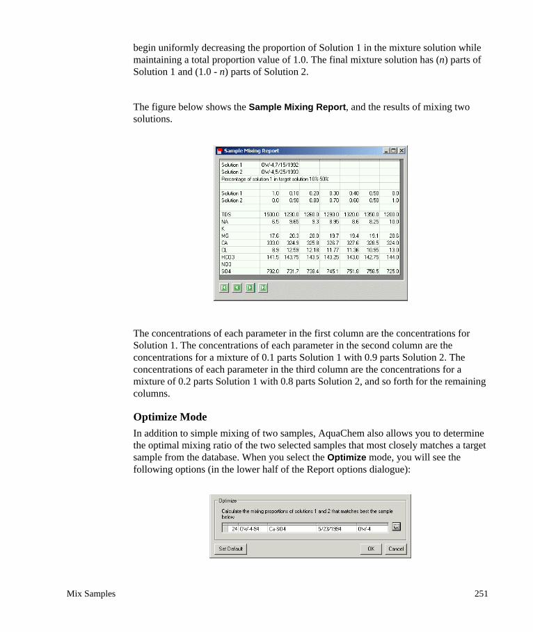
begin uniformly decreasing the proportion of Solution 1 in the mixture solution while maintaining a total proportion value of 1.0. The final mixture solution has (n) parts of Solution 1 and (1.0 - n) parts of Solution 2.

The figure below shows the Sample Mixing Report, and the results of mixing two solutions.

The concentrations of each parameter in the first column are the concentrations for Solution 1. The concentrations of each parameter in the second column are the concentrations for a mixture of 0.1 parts Solution 1 with 0.9 parts Solution 2. The concentrations of each parameter in the third column are the concentrations for a mixture of 0.2 parts Solution 1 with 0.8 parts Solution 2, and so forth for the remaining columns.

Optimize ModeIn addition to simple mixing of two samples, AquaChem also allows you to determine the optimal mixing ratio of the two selected samples that most closely matches a target sample from the database. When you select the Optimize mode, you will see the following options (in the lower half of the Report options dialogue):

Mix Samples 251

This mixing mode requires you to select a sample that you would like to match. AquaChem will mix the two initial samples in 2% increments until the Euclidean distance between the calculated mixture and specified resulting sample is minimized.

The Optimize mode can be used in a situation where you have three samples (ex. groundwater, seawater and freshwater) and you suspect that the groundwater is a mixture of the freshwater and the seawater. The Optimize mode can be used to estimate the percentage of freshwater and the percentage of seawater required to obtain the groundwater composition of selected parameters.

To generate a report with Optimize mode, select a sample from your database, and click [OK].

5.4 Water Quality StandardsThe Water Quality Standards report provides a list of all parameters which exceed at least one of the established Guideline/Tolerance levels for the selected sample. If your sample contains no exceedences, then this Report will be blank.

When you select this report, a Water Quality window similar to the one below will appear:

Each line of the report contains the Parameter, corresponding Unit, actual measured Value and guideline values (e.g. Maximum Contaminant level (MCL), Goal contaminant level (GCL), Aesthetic Objectives (AO)). Depending on the Guideline used, you may see one, two, or three guideline levels. The example above shows three levels, a maximum concentration limit, a tolerated concentration limit and a concentration goal. AquaChem allows the definition of multiple standards; the active

252 Chapter 5: Reports

standard used for detecting exceedences in this report is defined in the Preferences dialogue available under the File menu.

The scroll arrows in the lower left corner of the Report window can be used to produce a report for other samples in your database.

5.5 Rock Source DeductionThe Rock Source Deduction report allows you to gain insight into the possible origin of the water sample. The results are a general overview based on ion ratios found in a sample which are compared to ratios of the respective ions in reactive minerals. If results do not meet expectations, the result should be confirmed with more detailed study based on multiple samples, aquifer mineralogy analysis, modeling and with the use of plots.

When you select this report, the following Rock Source Deduction window will appear:

The following table provides a summary of the criterion for the Rock Source Deduction Report.

Rock Source Deduction 253

Parameter Attention Value Conclusion Comments

SiO2 (mmol) >0.5 Volcanic glass or hydrothermal water possible

The solubility of quartz at 20° is X mg/L.

HCO3-/SiO2 >10>5 and <10<5

Carbonate weatheringAmbiguousSilicate weathering

Low carbonate SiO2 ratios indicate, that these ions are released from silicate minerals, especially if TDS is low.

SiO2/(Na+K-Cl) <1>1 and <2>2

Cation exchangeAlbite weatheringFerromagnesian minerals

(Na+K-Cl)/(Na+K-Cl+Ca)

0.2 - 0.8<0.2 or >0.8

Plagioklas weathering possiblePlagioklas weathering unlikely

Na/(Na+Cl) >0.5

=0.5<0.5 TDS >500<0.5 TDS <500 and >50<0.5 TDS <50

Sodium Source other than halite - albite, ion exchangeHalite SolutionReverse Softening, seawaterAnalysis ErrorRainwater

Mg/(Ca+Mg) =0.5 and (HCO3/Si)>10<0.5>0.5

<0.5 and (HCO3/Si)<5>0.5

Dolomite WeatheringLimestone-Dolomite WeatheringDolomite Dissolution, calcite precipitation, or seawaterFerromagnesian MineralsGranitic weathering

Ca/(Ca+SO4) =0.5<0.5 and pH<5.5<0.5 and pH neutral

>0.5

Gypsum dissolutionPyrite oxidationCalcium removal - ion exchange or calcite precipitationCalcium source other than gypsum - carbonate or silicates

TDS >500<500

Carbonate weathering or brine or seawaterSilicate weathering

Cl/Sum Anions >0.8 and TDS>500>0.8 and TDS<100<0.8

Seawater or brine or evaporitesRainwaterRock weathering

HCO3/Sum Anions

>0.8>0.8 and SO4 >20meq/L<0.8 and sulfate low

Silicate or carbonate weatheringGypsum dissolutionSeawater or brine

254 Chapter 5: Reports

The report will complete the Parameter analysis, check the Attention Values, and produce a result value and Conclusion on the rock source.

If the report values shows “n/a”, it means that no data is available and the calculation could not be performed.

The scroll arrows in the lower right corner of the Rock Source Deduction Report window can be used to produce a report for other samples in your database.

For more details please see the reference below:

Hounslow, A.W. 1995. Water Quality Data – Analysis and Interpretation. CRC Press LLC. p.85.

5.6 StatisticsAquaChem comprises most of the commonly used statistical methods and techniques for the analysis of water samples:

• Summary Statistics• Correlation Matrix• Trend Analysis• Outlier tests, and• Tests for Normality

These analyses are available under Reports>Statistics and are discussed in detail below.

The statistics used in AquaChem were developed in accordance with USEPA guidelines outlined in the following document:

Guidance for Data Quality Assessment, Practical Methods for Data Analysis, EPAQA/G-9 QA00 Update. July 2000. USEPA Office of Environmental Information, Washington

5.6.1 Summary StatisticsThe Summary Statistics report calculates basic statistics for all active samples in your database. When you select Reports from the main menu, then Statistics, and, finally, Summary Statistics from the sub-menu, the following Statistics options dialogue will appear:

Calcite Saturation Index

>0=0<0

Oversaturated with respect to CalciteSaturated with respect to CalciteUndersaturated with respect to Calcite

Statistics 255

The above dialogue allows you to customize your summary statistics report using the available tabs. At the top of this dialogue is a combo box which allows you to choose a previously saved combination of settings.

In the first tab, Parameters, you must specify the parameters for which the summary statistics are to be calculated. Click the button to produce a standard parameter selection dialogue and choose the desired parameters by highlighting them and clicking [Select] button. When finished with parameter selection click [Close]. You can change the order of the chosen parameters by clicking the and buttons. Delete any

parameter by clicking the button.

Next, click on the Statistics tab.

256 Chapter 5: Reports

Use this dialogue to select the statistics for your data. Click the button to produce the following dialogue:

Scroll through the available list of statistics to select the desired ones. Click [Select] to add a chosen statistic. When finished, click [Close]. The statistic abbreviation will be listed in the Function column of the statistic list. The Title column lists the full statistic names and these names will appear as headers on the output. You can modify these entries by double-clicking in the cell and entering a new Title. You can change the order of the chosen statistics by clicking the and buttons. Delete any parameter

by clicking the button.

Once the statistics are chosen, you can modify some of their options in the Summary Statistics dialogue. To access statistic options simply highlight it in the list, and available options will be displayed in the bottom portion of the dialogue:

Statistics 257

AquaChem allows you to decide how to deal with censored data. The Censored Data combo box allows you to select the method used to manage non-detects. The options are Auto, Ignore, Multiply, Constant, Trimmed, Winsorize. Depending on the method chosen you may have to enter additional data (e.g. if you chose Multiply, you will have to enter the Factor to multiply by). Choosing Auto will subject the censored data to the method specified in the Preferences (for more details see “Non-detects” on page 91 in Chapter 3).

The following is a description of each Statistical Analysis available for this report:

MIN (minimum): lowest recorded value for the parameter

MAX (maximum): highest recorded value for the parameter

RAN (range): maximum minus minimum

IQR (interquartile range): Q75 minus Q25

MEAN (Arithmetic mean): average value for the parameter

STD (Standard Deviation): square root of the variance

2ss =

258 Chapter 5: Reports

QUANT (non parametric quantile): The Quantile is a data value, that is greater than or equal to a given fraction of the data values. If x is the p quantile, then at least the fraction p of the value set lie at or below x, at least 1-p of the value lie at or above x. For the non parametric quantile calculation no assumption is made for the underlying data set. The data is ranked from the lowest to the highest value. The quantile p is then calculated depending as follows

if number of points is odd:

if number of points is even:

CI (confidence interval): The confidence interval gives an estimated range of values which is likely to include the sample mean. The estimated range is calculated from a given set of sample data. Confidence intervals are usually calculated so that this percentage is 95%, but AquaChem can produce 90%, 99%, 99.9% (or any other) confidence intervals for the mean. The confidence range is calculated as the upper minus the lower confidence interval

DEV_COEF (Deviation Coefficient): Coefficient of Variance calculated using the formula below.

SKEW (skewness): skewness is calculated according to the following formula:

KURT (kurtosis): kurtosis is calculated according to the following formula:

)2/]1([~

+= nXX

2~ )1]2/([)2/( ++= nn XX

X

⎟⎠⎞

⎜⎝⎛

--⎟⎠⎞

⎜⎝⎛

+ ---- nstx

nstx nn 1,11,1 aa

s

X--- 100 %100=

xsCV

∑= ⎟

⎠⎞

⎜⎝⎛ -

--=

n

ii

i

sxx

nnnskew

)2)(1(

Statistics 259

N (number of samples): number of samples that have a measured value for the selected parameter.

N_ND (number of non-detects): number of samples that list the value for the selected parameter as a non-detect

PERC_ND (percent of non-detects): number of non-detects divided by the total number of samples and multiplied by one hundred

VAR (Variance): average square distance from points to sample mean

QUANT_PAR (parametric quantile): For the parametric quantile calculation the data is assumed to be normally distributed. A 0.25 quantile thus corresponds to the Z value of the normal distribution for a probability of 0.25.

N_EXC (number of exceedences): number of samples that have exceedences for the selected parameter

PERC_EXC (percent of exceedences): number of exceedences for the parameter divided by the total number of samples and multiplied by one hundred

N_D (number of detects): number of samples for which the selected parameter could be detected

PERC_D (percent of detects): number of detects for the parameter divided by the total number of samples and multiplied by one hundred

N_DBS (number of detects below standard): number of values below standard for the selected parameter

PERC_DBS (percent of detects below standard): number of detects below standard divided by the total number of samples and multiplied by one hundred

N_DAS (number of detects above standard): number of values above standard for the selected parameter

3)(

4

4

-∑ -

= =

snxx

kurtn

iii

∑=

--

=n

ii yy

ns

1

22 )(1

1

260 Chapter 5: Reports

PERC_DAS (percent of detects above standard): number of values above standard for the selected parameter divided by the total number and multiplied by one hundred

TSTAT (t-statistic): calculates t-statistic for the parameter

LCL (lower confidence limit): calculates lower confidence limit

UCL (upper confidence limit): calculates upper confidence limit

TI (tolerance interval): The tolerance interval is a way of determining a range that (with a certain confidence level) will contain a certain percentage of the population

LTI (lower tolerance limit): calculates lower tolerance limit

UTI (upper tolerance limit): calculates upper tolerance limit

MKS (Mann Kendall Statistic): indicates increasing or decreasing trend

MKZ: (Mann Kendall Statistic): approximates Z value for calculating probability

The next tab allows you to specify the output settings:

nstx n- -- 1,1 a

nstx n+ -- 1,1 a

Statistics 261

The Parameter as combo box allows you to set the parameter orientation. When Rows is selected, the parameters will be displayed in rows and statistics in columns. When Columns is selected, the orientations are reversed with parameters displayed in columns and statistics in rows.

AquaChem allows you to break the Summary Statistics output by symbol. When this option is selected, the statistics will be calculated and displayed for every symbol. Thus, if you have a symbol assigned to every sample, all samples with the same symbols will be grouped and statistics performed on those groups.

The Data tab provides you with a preview of data of the selected parameters:

If you are satisfied with the settings for the Summary Statistics report, before generating it, you may wish to save these settings by clicking [Save] button. The following Save dialogue will be loaded:

Type in a new name, or select an already existing name if you wish to update the settings. This dialogue also allows you to delete the settings that are no longer needed. Simply select the name of the settings you wish to delete and click the button.

Click [OK] to save the settings.

262 Chapter 5: Reports

Click [OK] to generate the report.

An example of a finished report if displayed below:

You may print this report, or save it in .XLS, .TXT, or .CSV format.

5.6.2 Correlation MatrixThe Correlation Matrix Report shows a simple correlation matrix of the parameters for the samples in your database. This allows you to quickly determine the similarities or differences between your samples. When you select Reports from the main menu and then Statistics>Correlation Matrix, the following dialogue will appear:

The Correlation Matrix Report requires you to specify parameters which will be used in the correlation analysis. To add new parameters, press the button and select a parameter from the available list. You can also include parameter ratios, sums or differences (e.g. Na/Cl, Ca+Mg, Cl-SO4) in the Parameters field; simply type these values in manually in the parameter field. To remove parameters from the list, press the button.

When the Use Selected samples only option is enabled, only the samples which are selected in the active list will be used. If this option is disabled, then all samples in the active list will be used.

The Unit field beside every parameter contains a combo box listing the available concentration units for the correlation of the chemical parameters. Units of mol/l are often more suitable for correlating than mg/L, because it gives you an idea as to which minerals have been dissolved.

Statistics 263

Once you have specified the required options, press [OK] and the report will be generated as shown in the figure below:

The Correlation Matrix report generates a correlation matrix for a specified number of sample parameters that are common to all samples. A linear regression routine calculates the regression coefficient (r), and the slope and intercept of the regression line.

The figure below shows the correlation of Ca against SO4 for three different scenarios.

])(

[])(

[1

1

2

2

1

1

2

2

1

1 1

∑∑

∑∑

∑∑ ∑

=

=

=

=

=

= =

--

-

=

n

i

n

ii

i

n

i

n

ii

i

n

i

n

i

n

iii

ii

n

yy

n

xx

n

yxyx

r

264 Chapter 5: Reports

The correlation of Ca and SO4 in three samples above is as follows:

(A) high positive correlation

(B) low positive correlation

(C) high negative correlation

It is often useful to check the correlation results graphically in a scatter plot to easily identify outliers which might influence the correlation result. The Scatter plot is available as one of the plot types, under the Plots menu. In the Scatter plot options, access the Edit Lines option under the Symbols tab. In this dialogue, you can calculate the regression curve. For more details, see Scatter Plot in Chapter 4.

The Correlation Matrix also includes the Spearman Rank Correlation coefficient. This value is calculates using the assigned rank, rather than exact values. This coefficient is useful when it is not economically feasible to obtain the exact values. Spearman Rank Correlation coefficient is a good indicator of a relationship between two variables, in case this relationship is not linear.

5.6.3 Trend AnalysisThe Trend Analysis option estimates a potential positive or negative trend that may be present in the data. A trend analysis may be interesting for three types of problems:

• When detecting an increasing trend becomes important to show that the contaminants in the down gradient wells increase with time and may eventually exceed its water quality standards.

• For compliance monitoring projects, the success of groundwater cleanup and remediation works can be verified by testing if the contaminant shows a decreasing trend.

• Finally, if a dataset is to be used in a test assumption of independent data, trend analysis can be used in order to ensure that this data does not include any trend at all.

CaA)

r = 0.9

CaB)

r = 0.2

CaC)

r = -0.9

Statistics 265

When you select Reports>Statistics>Trend, the following dialogue will appear:

The trend analysis screen contains the following elements: From the Method combo box select the desired regression method. The available methods are as follows:

• Linear Regression• Sen’s Test, and• Mann-Kendall Test

The Parameter box allows you to select the parameter which is used for the test. The Data tab shows values and the date of sampling for the specified parameter. Particular data points may be excluded from the test by unchecking the Use check box for this sample. The Plot tab shows time series plot for visual control. The results tab contains the Result of the test after pressing the [Calculate] button.

NOTE: There is also a [Copy] button at the bottom of the dialogue. This button allows you to copy the current result grid into the clipboard from where it may be pasted into any other application, for example MSExcel.

Linear RegressionThe linear regression simply calculates a regression line on the time/value plot. A positive slope of the regression line indicates a trend towards increasing values, a negative slope a trend to decreasing values. However the result of this test should only

266 Chapter 5: Reports

be used qualitatively and should be confirmed by more sophisticated tests such as Sen’s and Mann-Kendall. The calculated line is drawn on the time series plot.

Sen’s TestSen (1968) developed a simple nonparametric estimator of trend which is particularly useful for groundwater monitoring applications. The method is robust to outliers, missing data and non-detects. To compute the Sen’s trend estimator S, the individual slopes for any succeeding points are calculated. The trend estimator corresponds to the median of all calculated slopes. To calculate the confidence limits, an estimate of the variance of S is required which may be calculated using the following formula:

where q is the number of values for which there are ties and tp is the number of tied measurements for a particular value. The lower and upper confidence limit M1 and M2 can be calculated as follows:

The calculated ranks M1 and M2 are projected on the ranked slope data. If the respective interval contains the zero value, the Null Hypothesis of non trend is

⎥⎦

⎤⎢⎣

⎡+--+-= ∑

=

q

pppp tttnnnS

1)52)(1()52)(1(

181)var(

2)var(' 1

1SZN

M a--=

2)var(' 1

2SZN

M a-+=

Statistics 267

accepted. The Output of Aquachem includes the Median slope, the variance S, M1, M2 as well as their respective slopes. Both Hypothesis, “Increasing trend” and “Decreasing trend” are tested according to the specified probability and the result reported in the result table shown below.

For more details on the Sen’s test please see the reference below:

Gibbons, R.D., 1995: Statistical Methods for Groundwater Monitoring. p.175.

Mann-Kendall TestThe Mann-Kendall test is a trend estimator that can be used to prove if contaminant concentrations are significantly diminishing or rising over time. For this test, there are no distributional assumptions, and missing data (non-detects) or irregularly spaced measurement periods are allowed. Non-detects are assigned a value smaller than the smallest measured value.

The version of the Mann-Kendall Test used in AquaChem can be applied for virtually any groundwater parameter. The Mann Kendall test provides two values; S value and Z value. The test procedure is as follows:

First, order the data by sampling date x1, x2, ....,xn where xi is the measured value on occasion i.

Second, record the signs of each of the N’ possible differences xi’ -xi where i’ > i. For example, let

268 Chapter 5: Reports

sgn (xi’ -xi) = 1 if xi’ -xi > 0

= 0 if xi’ -xi = 0

= -1 if xi’ -xi < 0

The Mann-Kendall statistic (S) is then computed as:

which is the number of positive differences minus the number of negative differences.

If S = 0, then there is no increasing or decreasing trend in the data

If S < 0, then there is a decreasing trend, indicating concentration is decreasing over the time interval.

If S > 0, then there is an increasing trend, indicating concentration is increasing over the time interval.

A two-sided test (for either increasing or decreasing trend) can also be obtained, using probability values. For n > 10, then the normal approximation (Z) is calculated as follows:

If S > 0, then

If S = 0, then Z = 0

If S < 0, then

Where var(S) is calculated according to the formula used for the Sen’s slope estimator. The quantity Z can be compared to standard normal cumulative distribution probabilities to test the null hypothesis of no trend.

In the Statistics Report window, the S value is displayed as S(M-K), and the Z value is displayed as Z(M-K).

For more details on the Mann-Kendall test please see the reference below:

Gibbons, R.D., 1995: Statistical Methods for Groundwater Monitoring. p.178.

S xi¢ xi–( )sgni'=k+1∑

i 1=

n 1–

∑=

Z S 1–var S( )[ ]

0.5---------------------------=

Z S 1+var S( )[ ]

0.5---------------------------=

Statistics 269

After you have selected a test to use in trend calculation, select the parameter for which you wish to calculate the trend.

All stations will be displayed in the Data tab, sorted by date in ascending order. At this point you can de-select any samples you do not wish to use in the analysis. Simply un-check the box beside the sample to remove it from calculations.

Once you are satisfied with the data selection, move on to the Plot tab. This tab offers a graphical representation of the selected data.

270 Chapter 5: Reports

The graphical representation of the data is very helpful because it allows you to see if there are any outliers that may potentially distort the analysis.

Once you are satisfied with the view click the [Calculate] button, and the trend will be calculated and displayed in the result tab.

Depending on the chosen test, different results will be displayed, however one common entry is the Result line at the bottom of the list of calculated parameters. The result can be:

• increasing trend accepted/rejected• decreasing trend accepted/rejected

To see the calculations for another method and/or parameter simply change these options in their respective combo boxes and click [Calculate] again.

5.6.4 Outlier testsOutliers are measurements that are extremely large or small relative to the rest of the data and, therefore, are suspected of misrepresenting the population from which they were collected. Outliers may result from transcription errors, data-coding errors, or measurement system problems such as instrument breakdown. However, outliers may also represent true extreme values of a distribution (for instance, hot spots) and indicate more variability in the population than expected. Not removing true outliers and removing false outliers both lead to a distortion of estimates of population parameters. (Office of Environmental Information, U.S. Environmental Protection Agency, 2000).

Selecting this option from the Statistics sub-menu launches the following dialogue:

Statistics 271

At the top of the dialogue, there is a combo-box which allows you to choose from four available outlier tests:

• Dixon’s Extreme Value Test• Discordance Test• Rosner’s Test• Walsh’s Test

Each of the above test carries with it certain assumptions which are listed below the combo box in the Assumptions frame. A description of these tests together with directives for the calculations can be found in the USEPA report QA/G-9> Guidance for Data Quality Assessment.

When you select a particular test, the level of Significance is filled in automatically with the available values that may be used for this test.

Many statistical tests require that the underlying dataset is normally distributed. However in detection monitoring, data is frequently log-normally distributed. This means that if the log of all values is plotted, the dataset will have a normal distribution. Outlier tests requiring normal distribution may be performed on such datasets, if the lognormal transformation is activated.

Once you have set the test particulars and are satisfied that your data meets the assumptions, select the desired test parameter using the combo box provided.

Below the setting frame there are three tabs: Data, Histogram and Results. The Data tab displays all values available for the selected parameter in ascending order as well as the arithmetic mean, standard deviation, and the number of samples. The number of samples is especially useful as it sometimes helps you determine which test to use. The

272 Chapter 5: Reports

Histogram tab displays the data in a histogram plot and allows a visual control of the calculated results.

Once you are satisfied with the selected test and parameter, move to the Results tab and click the [Calculate] button.

Depending on the selected test, the output may be slightly different. Below is a sample of the output of the Discordance Test:

If one or several outliers are detected, you will be prompted whether this data should be marked as outliers in your database.

If confirmed, the respective measurements will be marked as an outlier in the database and a message similar to the following will appear:

The value will remain in the database but it will be ignored for any calculations or plots. The outlier column of the sample detail screen will show a marked check box for this

Statistics 273

parameter. Use the Highlight Outliers menu item from the Tools>QA/QC submenu in order to highlight all samples containing values marked as outliers.

5.6.5 Tests for NormalityMany statistical tests and models are only appropriate for data that follow a certain distribution, in particular, the assumption of normality. There are many methods available for verifying the assumption of normality ranging from simple to complex. As recommended by the USEPA Guidance for Data Assessment document, there are five of the more common tests are built into AquaChem.

Selecting this option from the Statistics sub-menu launches the following dialogue:

At the top of the dialogue there is a combo box which allows you to select a test to perform a lognormal transformation of the data. The available tests are:

• Studentized range test (t-test)• Geary’s test• Shapiro-Wilk Test (W-test)• d’Agostino’s test, and• Coefficient of Variation

Each of the above test carries with it certain assumptions which are listed below the combo box in the Assumptions frame. A description of these tests together with

274 Chapter 5: Reports

directives for the calculations can be found in the EPA report QA/G-9 Guidance for Data Quality Assessment, sections 4.2 and following.

When you select a particular test, the level of Significance is filled in automatically with the default value used for that test. However, you may change this value using the combo box provided.

Below the settings frame there are three tabs: Data, Histogram and Results. The Data tab displays all values available for the selected parameter in ascending order as well as the arithmetic mean, standard deviation, and the number of samples. The number of samples is especially useful as it sometimes helps you determine which test to use.

You may also see the data graphically, in the form of a Histogram:

Once you are satisfied with the selected test and parameter click the [Calculate] button.

Depending on the selected test, the output may be slightly different. Below are the results for Coefficient of Variance test:

Statistics 275

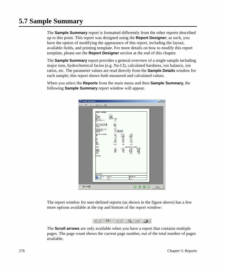
5.7 Sample SummaryThe Sample Summary report is formatted differently from the other reports described up to this point. This report was designed using the Report Designer; as such, you have the option of modifying the appearance of this report, including the layout, available fields, and printing template. For more details on how to modify this report template, please see the Report Designer section at the end of this chapter.

The Sample Summary report provides a general overview of a single sample including major ions, hydrochemical facies (e.g. Na-Cl), calculated hardness, ion balance, ion ratios, etc. The parameter values are read directly from the Sample Details window for each sample; this report shows both measured and calculated values.

When you select the Reports from the main menu and then Sample Summary, the following Sample Summary report window will appear.

The report window for user-defined reports (as shown in the figure above) has a few more options available at the top and bottom of the report window:

The Scroll arrows are only available when you have a report that contains multiple pages. The page count shows the current page number, out of the total number of pages available.

276 Chapter 5: Reports

The Zoom (magnifying) button allows you to change the zoom size of the window. When you press the down arrow beside the magnifying glass, you will see several window size options. Simply choose the desired zoom size and the preview window should be automatically refreshed.

The Print button sends the reports for all selected samples to the printer.

The Show fields option is only available if the Report is linked to a printing template (done using the Report Designer). To enable this option, place a check mark in this box. You will then see the following dialogue appear in the middle of your display, to the left of the preview window:

In these fields, you can enter the appropriate descriptive information that should appear in the template. As the information is entered, the report preview window should be automatically updated.

The Scroll arrows on the bottom of the report window are only available when only one sample is selected. They allow you to scroll through the entire dataset.

NOTE: You may generate single-page and multi-page reports. Selecting multiple samples and generating a Sample Summary report will generate an individual report for each selected sample, allowing you to scroll through them using the scroll buttons at

Sample Summary 277

the TOP of the report window. Printing the report at this stage will print a report for ALL selected samples. Alternately, if you generate the Sample Summary report while only one sample is selected, the report will be created for that samples and you will be able to scroll through all samples in the project using the green scroll buttons at the BOTTOM of the report window. Printing the report will produce a printout of this sample ONLY.

Clicking the [Close] button closes the report.

This report will be edited in Report Designer.

NOTE: When you save user-defined reports, the report template information will not be saved; only the report contents are saved to a file.

5.8 ThermometersThis report lists the geochemical thermometers and their estimated temperatures which are calculated using the formulas defined in the Thermometers tab of the Database. This report may be edited in Report Designer.

5.9 Isotopes

This report lists the concentrations of isotopes 18O and 2H as well as infiltration temperature and height for 18O which are calculated according to formulas specified in Calculations tab of the Database. This report may be edited in Report Designer.

5.10 Report DesignerAs mentioned earlier in this chapter, AquaChem allows you to create two types of reports:

• The pre-defined (hardwired) reports, and • The user-defined reports

The hardwired reports cannot be modified, nor can their layout be changed. These reports include: Compare Sample, Mix Samples, Water Quality Standards, Reliability Check, Compare Duplicates, Rock Source Deduction, Summary Statistics, and Correlation Matrix.

278 Chapter 5: Reports

The user-defined reports (ex. Sample Summary) can be modified using the Report Designer.

Using the Report Designer you may design and customize up to 10 new reports for your own project needs. The report may include any combination of database parameters and function (calculation) results. Once a new report has been created, it can be selected from the Reports menu, below the Isotopes report.

5.10.1 General FeaturesWhen you select Report Designer from the Reports menu, the following dialogue will appear. The Report Designer dialogue is separated into three tabs: Reports, Edit, and Preview.

ReportsProvides a list of the reports available in the current database template, and general information on each report (Description, Selected Printing template, report size, and selected font).

Edit Provides options for designing the report layout.

Report Designer 279

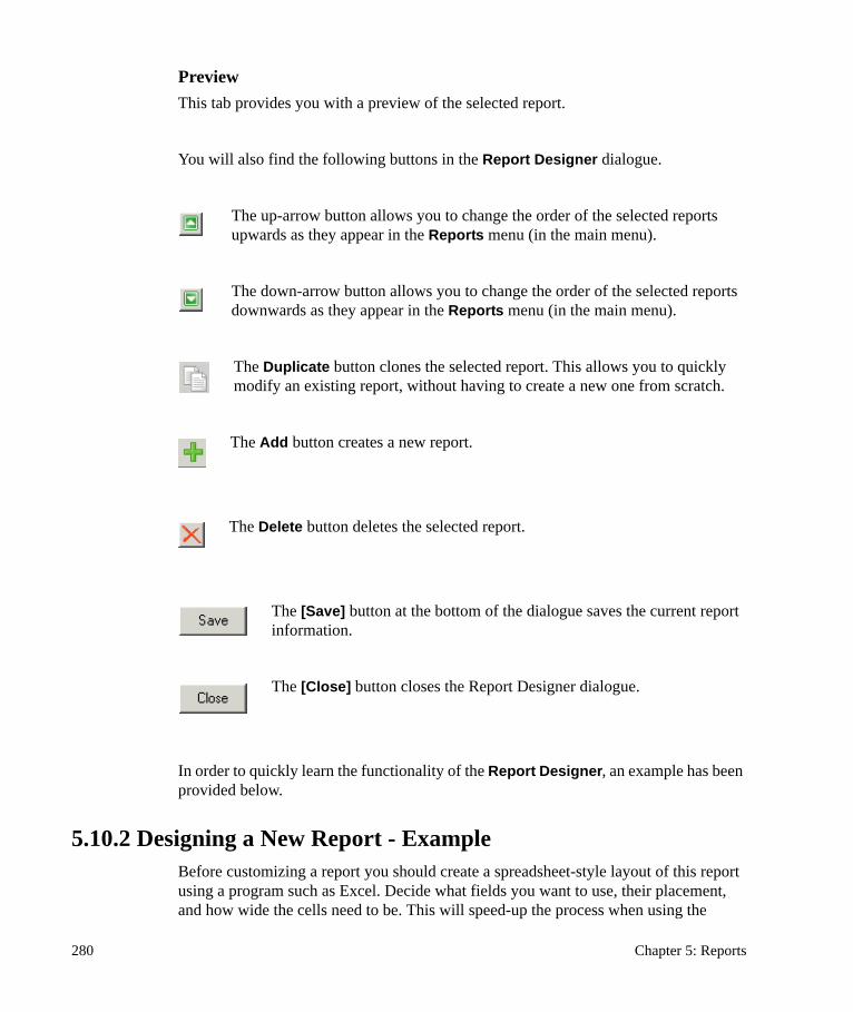
PreviewThis tab provides you with a preview of the selected report.

You will also find the following buttons in the Report Designer dialogue.

The up-arrow button allows you to change the order of the selected reports upwards as they appear in the Reports menu (in the main menu).

The down-arrow button allows you to change the order of the selected reports downwards as they appear in the Reports menu (in the main menu).

The Duplicate button clones the selected report. This allows you to quickly modify an existing report, without having to create a new one from scratch.

The Add button creates a new report.

The Delete button deletes the selected report.

The [Save] button at the bottom of the dialogue saves the current report information.

The [Close] button closes the Report Designer dialogue.

In order to quickly learn the functionality of the Report Designer, an example has been provided below.

5.10.2 Designing a New Report - ExampleBefore customizing a report you should create a spreadsheet-style layout of this report using a program such as Excel. Decide what fields you want to use, their placement, and how wide the cells need to be. This will speed-up the process when using the

280 Chapter 5: Reports

Report Designer in AquaChem. Below is the layout that will be used for this simple example report.

To create a new report, follow the steps as described below.

If you have not already done so, load the Report Designer from the Reports menu. Ensure you are viewing the Reports tab (the first tab).

Report Designer 281

button to create a new report. A new line will be added below the Isotopes Report, with the name: #New Report.

#NewReport and enter a name for this new report.

type: Example

<Enter> (on your keyboard)

In the lower half of this dialogue:

type: An Example Report (in the Description field)

‘none’ for the Template

type: 20 (the Number of Rows for this report)

type: 5 (the Number of Columns for this report)

button to change the Default Font for this report

Times New Roman / Regular / 10 font size

[OK]

[Save] (in the lower right corner of the dialogue) to save this report.

You can now proceed to add fields to this report.

Edit tab (from the top of the dialogue).

282 Chapter 5: Reports

This will present you with a blank grid (spreadsheet), containing 20 rows and 5 columns as shown below.

You will see that the rows are numbered and the columns are lettered (similar to MSExcel) to allow you to quickly locate cell locations in the grid. At this point you may begin to add values to the cells. You may fill cells with text, database parameters, or with a function (calculation).

Double-click on the cell in the upper-left corner (Cell A1) and the Cell dialogue (as shown below) will appear:

Report Designer 283

This dialogue allows you to control the contents of the selected cell. Cell contents must be assigned one cell at a time. Below are the options available for each cell:

TypeClick on the button and you may choose from the following cell types:

Text: Enter the desired text for the cell

Sample Description: choose from a list of Sample Description parameters

Station Description: choose from a list of Station Description parameters

Measured/Modeled Value: choose from a list of Measured or Modeled parameter values.

Ratio: choose two parameters to show as a ratio

Guideline Level1: displays the current guideline level 1 for the specified parameter

Guideline Level2: displays the current guideline level 2 for the specified parameter

Guideline Level3: displays the current guideline level 3 for the specified parameter

Function Value: choose from a list of available calculations

Range Name: select from a list of available Ranges

Thermometers: select from a list of Geothermometers

Span nextThis option is useful for headings and titles, where the text may not fit into one cell. If the cell to the right of the selected cell is empty, you may span several cells into one. Simply enter a cell number in this field (ex. Span 2 cells).

AlignmentChoose from Left, Center, or Right-Justified.

The three fields described above are common to all data types listed. Below, all data types are listed along with the descriptions of the other fields that go with them.

284 Chapter 5: Reports

Text

TextEnter the text you wish to appear in this cell. Used for captions that do not change (e.g. “Station ID”)

Sample Description

Sample ParameterUse the combo box to select a sample parameter. The value of this cell will change depending on what sample is loaded into the report.

Station Description

Station ParameterUse the combo box to select a station parameter. The value of this cell will change as you move between samples that are assigned to different stations.

Measured/Modeled Parameter

ParameterUse the combo box to select a measured or a modeled parameter. The cell will reflect the value of this parameter for the sample that is loaded into the report.

UnitUse the combo box to select a unit for the parameter (becomes inactive if the chosen parameter is unitless - e.g. pH).

FormatUse the combo box to select the numeric format for the parameter value.

Ratio

NumeratorUse the combo box to select the parameter to serve as the numerator of the ratio.

DenominatorUse the combo box to select the parameter to serve as the denominator of the ratio.

Report Designer 285

UnitsUse the combo box to select the units for the parameters used as the numerator and the denominator. The ratio may change depending on the chosen units (e.g. the ratio of the parameter values in g/l will be different from the ratio of the parameter values in mol/l)

FormatUse the combo box to select the numeric format for the ratio.

Guideline Level 1, 2, and 3

Guideline LevelUse the combo box to select the parameter for which the selected guideline level will be displayed. The value of the cell will stay the same regardless of the sample loaded into the report.

FormatUse the combo box to select the format for the cell value.

Function Value

FunctionUse the combo box to select a function, the result of which will be displayed in the cell. The functions are defined in the Calculations tab of the Database.

UnitUse the combo box to select the unit for the parameters used in the function. The result of the calculations may be different depending on the units used.

FormatUse the combo box to select the format for the result value.

Range Name

ParameterThe combo box lists the parameters that have the range(s) defined. The cell will display the name of the range that contains the value of the specified parameter for the current sample (e.g. Natural aquifer range).

286 Chapter 5: Reports

Thermometer

ThermometerUse the combo box to select the thermometer function. The thermometer calculations are defined in the Thermometers tab of the Database.

“Designing a New Report” continuedYou will now enter a Report Title for cell A1:

Text (from the list beside the Type field)

type: 1 in the Span next ... cells field

Left justify, for the cell alignment

type: General Report (beside the Text field)

[OK]

You should now see an entry under the Edit tab for Cell A1. You may switch to the Preview tab to see a preview of how the report will appear.

As you can see, the words take up two lines in the cell. To have the words fit on one line you can span this cell into the adjacent one.

Report Designer 287

Switch back to the Edit tab

Double-click on the cell A1 to produce the Cell dialogue

type: 2 in the Span the next ... cells

Switch to the Preview tab again. Now it should look similar the picture below (use the magnifying glass menu to adjust the view size):

The text colors of the cells in the Edit dialogue are representative of the cell types. The following summary provides a list of what each cell color indicates of the cell type:

Black: Text cells

Green: Sample and Station Description parameters

Blue: Measured and Modeled parameters, and Parameter Ratios

Grey: Function (Calculated) values, Thermometers, and Ranges

Red: Guideline Levels

If you want to change the column widths, simply drag the column to the desired width in the spreadsheet. Alternatively, you can select the column then right-click the highlighted column and select Set Column Width. Enter the precise value of the column width in the pop-up dialogue and press [OK]. Then load the Preview window to see the refreshed report.

The font for the report may be customized in two places:

In the Reports tab, the Default Font for the entire report is defined; all items on the report will use this font, size and style.

288 Chapter 5: Reports

A default font may also be assigned on a per row basis. To do so, select an entire row and right-mouse click on it and select Font. Select the desired Font from the dialogue that appears, and click [OK]. This font will be applied to an entire row. This is practical for assigning fonts to column headings in the report.

You can also insert and delete any selected row, column, or cell by highlighting the desired element, right-clicking on it, and choosing the appropriate action.

You will now proceed to define the remaining cells in the report, as per the pre-designed layout:

Cell A3

Select Text from Type field

type: Sample ID

[OK]

Cell A4

Select Text from Type field

type: Sampling Date

[OK]

Cell A5

Select Text from Type field

type: Location

[OK]

Using the same procedure, fill in the remaining text fields as per the layout above, in the appropriate cell locations:

Cell Text Entry

A7 Major Ions

A9 Ca

A10 Mg

Report Designer 289

A11 Na

A13 Sum Anions

A14 Ion Balance

A16 Ratio

A18 Na/Cl

B8 mg/l

B16 mg/l

C9 Cl

C10 SO4

C11 HCO3

C13 Sum Cations

D8 mg/l

Click on the Preview tab to see if any caption is too big for its cell. Go back to the Edit tab and if there were such captions, resize the column they are in so that they only take up one line. Do not worry if some parameter names (such as “SAMPLE_DATE”) take up a lot of space - gauge the length of the value.

Once you are finished you should save the changes that have been made so far.

[Save] in the lower-right corner of the Report Designer dialogue, to save the report design changes up to this point.

You can now add in the parameter value cells and function values.

Cell B3

Sample Description from the combo box beside cell Type

SAMPLEID from the combo box beside Sample Parameter field

[OK]

Cell B4

Sample Description from the combo box beside cell Type

Select SAMPLE_DATE from the combo box beside Sample Parameter field

290 Chapter 5: Reports

[OK]

Cell B5

Station Description from the combo box beside cell Type

Select LOCATION from the combo box beside Station Parameter

[OK]

Notice the color of the cells under the Edit tab in the Report Designer dialogue for these new cells; green cells indicate that these cells contain Station/Sample Description parameters.

Cell B9

Measured /Modeled Value from the combo box beside cell Type

Ca from the combo box beside Parameter

mg/l from the Unit field

[OK]

Cell B10

Measured Modeled Value from the combo box beside cell Type

Mg from the combo box beside Parameter

mg/l from the Unit field

[OK]

Cell B11

Measured Modeled Value from the combo box beside cell Type

Na from the combo box beside Parameter

mg/l from the Unit field

[OK]

Notice the color of the cells in the Edit dialogue; blue cells indicate that these cells contain Measured values.

Report Designer 291

Repeat this step for the remaining ions by choosing the appropriate parameter and placing this in the cell immediately beside the text cell for that parameter.

Cell Measured Value

D9 Cl

D10 SO4

D11 HCO3

Once you have finished this step, your display should be similar to the one shown below:

[Save] in the lower-right corner of the Report Designer dialogue to save the report design changes up to this point.

You will now add function values for the Sum Anions, Sum Cations, and Ion Balance

Cell B13

Function Value from the combo box beside cell Type

Left Justify from the Alignment field

292 Chapter 5: Reports

Select Sum of Anions from the combo box beside Function

[OK]

Cell D13

Function Value from the combo box beside cell Type

Left Justify from the Alignment field

Select Sum of Cations from the combo box beside Function

[OK]

Cell B14

Function Value from the combo box beside cell Type

Left Justify from the Alignment field

E. N. (Electroneutrality) from the combo box beside Function

[OK]

Notice the color of the cells in the Edit dialogue; grey cells indicate that these cells contain Function (Calculated) Values. Finally, you will add a Ratio to Cell B18 showing a parameter ratio of Na / Cl.

Cell B18

Select Ratio, from the combo box beside cell Type

Na for the first parameter

Cl for the second (right) parameter

mg/l for the units

Report Designer 293

[OK]

Notice the color of the cells in the Edit dialogue; blue cells indicate that this cell contains a Parameter Ratio.

[Save] in the lower-right corner of the report designer dialogue to save all changes to this report.

Once you have designed the report, click on the Preview tab to see a page preview.

This concludes the steps required to design a report. Feel free to add new cell values, functions, parameters, etc. in order to see the full capabilities of the Report Designer.

Once you are finished in the Report Designer, press [Close] to return to the main window of AquaChem. The newly created “Example Report” will now be available under Reports in the AquaChem main menu.

Edit Tab Preview Tab

294 Chapter 5: Reports

6Tools

The Tools menu provides access to the AquaChem data analysis tools, including Converters, Calculators, LookUp Tables, and access to the PHREEQC modeling interface.

The following Calculators and Converters are available:

• AquaChem Function• Decay Calculator• Find Missing Major Ion• Formula Weight Calculator• Volume Concentration Converter• Special Conversions• Species Converter• Unit Calculator• Calculate facies• Corrosion & Scaling• Oxygen Solubility

The following QA/QC checks are available:

• Reliability Check• Compare Duplicates• Find Duplicates• Highlight Nondetects• Highlight Outliers• Highlight Duplicates

The following LookUp Tables are available:

• Degradation Rates

295

• PHREEQC Phases• Periodic Table• Links• Organic Compounds• Preservation Methods

Finally, under the Modeling options you may:

• Calculate Saturation Indices and Activities• Calculate pH• Calculate Eh• Alk > HCO3, CO3• Equilibrate with Minerals• Run a PHREEQC (Basic) Simulation• Run a PHREEQC (Advanced) Simulation

6.1 Calculators and Converters

6.1.1 AquaChem FunctionThis tool allows you to quickly calculate any of the AquaChem built-in functions. Calculations can be performed without having to add/remove individual functions to the options of the Sample Details window.

To use this tool, first select a sample from your Active Samples list. Then select Calculators > AquaChem Function from the Tools menu, and a dialogue will appear as shown to the right side.

In this dialogue, you can see a Description of the function and the function units. By clicking on the down-arrow key, choose a function and then Format, and you will see the resulting value displayed in the Result field.

Use the arrows to move through the samples.

The calculations can be customized in the Calculations section of the Database options dialogue under the File menu. In here, you may select which calculations should appear in the AquaChem functions (calculations) lists.

296 Chapter 6: Tools

6.1.2 Decay CalculatorThe Decay Calculator allows you to calculate the concentration of a contaminant at a particular point in time following a specified rate of decay, or the time to reach a specified concentration based, again, on that decay rate. AquaChem also allows you to calculate the decay rate of a chemical based on two or more concentration-time pairs. Degradation rate of a contaminant is usually given as a "half-life", which is the time required for the substance to be reduced to half of the initial mass. This tool can be applied only to organic chemical parameters in your database. The formula for the rate of decay is as follows:

C0/C1 = e-kt

Where,

t = time

C0 = initial concentration

C1 = concentration after time t

When you access this tool, the following Decay Calculator dialogue will appear. The components of this dialogue are described below.

Sample

At the top of this dialogue under the Sample field, click on button and then double-click in Pick a sample list to select a sample for which you would like to run a

Calculators and Converters 297

degradation analysis. Selecting a sample from the sample list copies the concentration value for the current parameter to the initial concentration field C(t=0).

Parameter

In the Parameter field, click on the button and select the organic parameter you would like to analyze (please ensure that your sample contains a value for this organic parameter). Note that the parameter list contains all database parameters, which have a corresponding record in the Degradation Rates table (available under Tools > LookUp Tables).

Half-LifeAfter selecting a parameter, the Half-Life field will be automatically filled in with the appropriate value. The combo box to the right of the Half-Life field provides options for the Half-Life environments (Soil, Air, Groundwater, and Surface water) for which degradation rates are specified in the database. If all rates are known for these environments the list will contain a high, low, and average half-life values for each environment. Effects such as dilution, transport or adsorption etc. are not taken into account with this tool.

AquaChem includes values for 335 organic chemicals. These are taken from the following Reference:

Howard, P.H. et al., 1991: Handbook of Environmental Degradation Rates, Lewis Publishers, 775 p.

This tool may also be used as a simple degradation calculator, without selecting samples or parameters. Simply enter a Half-life value manually, choose your Problem Type, enter an initial concentration, target concentration or time period and press Calculate.

AquaChem also allows you to estimate a chemical’s half-life based on two or more time-concentration pairs.

Time UnitHalf-life values in the AquaChem database are saved as hours, however, you may convert these to days or years by selecting the appropriate Time Unit from the combo box.

Concentration UnitAllows you to select the concentration units that will be used in the half-life calculations.

298 Chapter 6: Tools

Problem TypeIn the next line, you must specify the Problem Type for the degradation calculator. The Decay Calculator has three problem types available:

Type 1: Time to reach a specified concentration

Type 2: Concentration after a specified amount of time

Type 3: Estimate half life from given concentration values

NOTE: If problem type 1 is selected, and the current contaminant has an assigned guideline level in your AquaChem database, a combo box with available guideline levels will appear to the right of the target concentration field. You have the option to choose the desired guideline level, and the C1 value will be automatically filled in for you.

A summary of the required data input is as follows:

Problem Type 1 In Problem Type 1 you can determine the time required for a contaminant to decay to a specified concentration.

C(t=0): initial concentration

C1: target concentration

Press [Calculate] and the t(C1) (time to reach target concentration) will be calculated.

Problem Type 2 In Problem Type 2 you can determine the concentration after a specified amount of time.

C(t=0): initial concentration

t1: target time

Press [Calculate] and the C(t1) (concentration after a specified time) will be calculated.

Calculators and Converters 299

This calculator accounts only for degradation effect, using the following equation:

C(t) = C1*e-kt

where,

k = residence time

Problem Type 3 In Problem Type 3 you can estimate half life from given concentration values.

Set the Parameter to “Custom”

Time: time of sampling

Conc.: concentration at sample time

Click [Calculate] to calculate the half-life as the slope of the regression line through the specified points. For every specified point, the estimated concentration by means of the linear regression line is displayed to verify the quality of the calculated values. At the left hand side of the screen, the estimated initial concentration, half-life, and the regression coefficient are displayed.

You can edit the concentration-time pairs at any time by double-clicking in the cell that contains the value you wish to edit. To remove the concentration-time pair highlight any cell in that pair and click the button.

6.1.3 Find Missing Major IonIf information for one of the major anions or cations (Na, Ca, Mg, Cl, HCO3, SO4) is missing from a sample, you can use this tool to estimate the concentration of the missing major ion. The concentration of the missing ion is calculated using the assumption that the total concentration of cations in meq/l is equal to the sum of anions. The entire difference of charges is assigned to the missing parameter.

NOTE: This tool is only available when you have a Sample Details window open and active.

Open a sample, and select Tools > Calculators > Find Missing Major Ion > Na (for the example shown below).

300 Chapter 6: Tools

After you have selected the desired missing parameter, AquaChem will calculate the missing value and display a confirmation message as shown on the right. Click [Yes] to accept the calculated value, or click [No] to reject the calculated value.

This tool does not work if more than one of the major cations or anions is missing in the analysis. In order to calculate the missing values for one of the major ions, each of the remaining major ions must be present.

If there is an over-abundance of the missing ion’s charge (e.g. Cl concentration is missing, the sample has already an anion excess) the following message will be displayed:

6.1.4 Formula Weight CalculatorThis tool allows you to quickly calculate formula weights for a user-specified chemical formula.

When you access this tool, the Calculate Formula Weight dialogue will appear. Simply enter the desired formula, and press [Calculate].

Note that the Formula is case sensitive; therefore, ensure that you enter two-letter elements such as Silicon as Si and not SI. In addition, only one level of parentheses is taken into account. So, in case of a formula with two levels of parenthesis such as

Calculators and Converters 301

((XY2)3)3AC, it will not be calculated correctly. In the standard display, simply the weight of the specified formula is calculated.

When checking the Extended checkbox, more options become available to convert different types of concentrations. This is convenient for converting PHREEQC results, expressed as mol/kg into mg/l. To do so, first enter the formula of the chemical. Then copy the PHREEQC molality value into the respective field, check the radio button and press the calculate button. The radio button tells the system that this field has been entered manually, and that all other concentration fields should be recalculated based on this value, the formula weight of the chemical, the density of the solution and the activity coefficient. this option may also be used to convert mg/L concentrations into ppm, provided that the density of the solution is known.

6.1.5 Volume Concentration ConverterThis converter allows you to quickly convert volume concentrations into mass concentrations for gas species, which are frequently reported in either of the two units.

When you access this tool, the Volume Concentration Converter dialogue will appear. Simply choose the observed ambient Temperature (0, 20, or 25oC), enter a Formula for an organic chemical, and enter the concentration. You may enter the concentration in either the ppmV or the mg/m3 field.

Press [Calculate] and the missing concentration will be calculated.

In the vapor phase, one ppm by volume (ppmV) is on a volume per volume bases. For example, one ppmV of Benzene in the air means one part volume of benzene in one million parts volume of air space. To convert the ppmV into mass concentration units (mg/m3), the following formula can be used:

302 Chapter 6: Tools

1 ppmV = FMW/K

where,

FMW = Formula Weight (g/mol)

K = is a temperature dependant coefficient (molar gas volume).

K= 22.4 l/mol at 0°C,

K= 24.05 l/mol at 20°C, and

K= 24.5 l/mol at 25°C.

Example:

To convert 1ppmV Benzene to mg/m3 at 20oC:

Mass Benzene mg/m3 = 1ppmV Benzene * [ (78 g/mol) / (24.05 l/mol) ]

= 3.24 g/L

= 3.24 mg/m3

NOTE: The formula is case sensitive, therefore, ensure that you enter two-letter elements such as Silicon as Si and not SI. In addition, only one level of parentheses is taken into account (i.e. a formula such as ((XY2)3)3AC will not be calculated correctly).

6.1.6 Special ConversionsThis tool provides conversions for numerous non-linear geochemical calculations. You may convert values from one measurement unit to another for measurement units such as pe - Eh, Alkalinity - HCO3, and Conductivity (us) - Resistivity (Ohm/cm).

When you access this tool, the Special Conversions dialogue will appear. Click on the button and choose a category from the list, enter the start value, and any other required variables (temperature, density), and press to convert the value.

The available conversion categories include:

Calculators and Converters 303

Conductivity Resistivity

where,

Cond =1/(Resistivity/1E+6)

Electrical conductivity at a different temperature: Cond(T1) Cond(T2).

It requires you to enter a conversion temperature. The conductivity is always normalized to a specific temperature which is dependant on the probe. If you want to enter conductivity data to your database, and the temperature for the probe is different (e.g. 25°C) from the one in the database (20°C) then the data has to be converted before being adding to the database.

This calculation is done in two steps:

• First, calculate the conductivity at standard temperature, • Second, calculate the conductivity at the specified temperature (Temp2).

Examples:

ConductivityCond(25) = Cond(Temp1) / (1 + 0.0198 * (Temp1 - 25))

Cond(Temp2) = Cond(25) * (1 + 0.0198 * (Temp2 - 25))

Redox potentialpe Eh

It requires you to enter an observation temperature.

pe(Eh): pe = Eh * F / 2.303 / R / T

Eh(pe): Eh = pe * 2.303 * RT / F

where,

R = 8.314 (Gas constant)

F = 96485 (Faraday constant)

Reference: C.A.J. Appelo, 1996: Geochemistry, Groundwater and Pollution, Balkema Roterdam, p. 246.

304 Chapter 6: Tools

Alkalinity calculationsConvert between:

mg/L HCO3,

meq/L,

Alkalinity (f*), where * means French degrees,

Alkalinity (g*), where * means German degrees

mg/L CaCO3.

Reference: John D. Hem. Study and Interpretation of the Chemical Characteristics of Natural Water, USGS Water supply paper 2254, p. 158.

Other conversionsppm mg/L: Requires you to enter a density.

mg/L = ppm / Density

mg/L ppm: Requires you to enter a density

ppm = mg/L * Density

6.1.7 Species ConverterThis tool allows you to convert any aqueous species into a different form. When you access this tool, the Species Converter dialogue will appear as shown below:

• Select a Master Element (Parameter) in which you are interested (common examples include nitrogen, phosphorus, silica, etc.).

• Type in a Source Species.• Type in a Target Species.• Enter a concentration of the source species in the lower left corner of the

dialogue.• The Conversion Factor is calculated based on the formula weights of the two

species: the Target species divided by the Source Species.

Calculators and Converters 305

• Press [Calculate] and the concentration for the target species will be calculated.

This tool is practical for expressing a measured amount of a parameter as different aqueous species when expressed in mg/L. For example, you may receive your Silica results as mg/L Si, and your database requires mg/L SiO2 or H2SiO3. For this you need to calculate the amount of SiO2 that holds the same amount of Silica as given in the lab analysis. Nitrogen species such as nitrate and nitrite may are commonly expressed as N or as their actual formula (NO3 or NO3) and constitute another good example where the above calculation may be useful.

The data entered in the Species Converter dialogue (shown above) depicts an example for converting Si species.

NOTE: The Formula is case sensitive; therefore, ensure that you enter two-letter elements such as Silicon as Si and not SI. In addition, only one level of brackets is taken into account (i.e. a formula such as ((XY2)3)3AC will not be calculated correctly).

6.1.8 Unit CalculatorThis tool performs basic unit conversions for length, time, volume, density, mass, etc.

When you access this tool, the Unit Calculator dialogue will appear as shown below.

Click on the button and select the desired category from the combo box at the top of the dialogue, enter the value and units in the fields below, and the new value will be automatically calculated.

In addition, you can modify the existing conversion factors, or create new ones. Press the [Options] button, and the following dialogue will be loaded.

306 Chapter 6: Tools

Select the Unit Type from the combo list (at the top), or press the button to load a list of available unit types, and options to create a new unit type. The list below will now show all conversions available for this unit type, and the conversion factor associated with each. You may enter or edit all factors, or create new conversions using the button. Then enter the appropriate conversion type and factor for this new conversion.

Once you are finished, press [Save] to save any changes you made to the conversions.

Press [Close] to return to the Unit Calculator tool.

6.1.9 Calculate faciesThis command calculates the Watertype (water facies) expression for all highlighted samples. The following dialogue allows you to chose the algorithm to be used in the calculation and the field where the calculated value will be placed:

The Mode lets the user select whether he wants to use the long facies name, which is based on the ions that contribute more than 10% (e.g. Ca-Mg-Cl-SO4), or the short mode, listing just the most frequent anion and cation.

Calculators and Converters 307

The Fill calculated watertypes into field combo box allows you to specify the target field where the value should be stored. Every sample must contain a field which contains the watertype and which is automatically recalculated if any changes to chemical concentrations occur, however the user may specify a second field, holding the water type in short notation. This can be useful when creating symbols based on watertypes. To implement this, use he Calculate facies command and select the Short version in the Mode combo box. Then, specify a field other than the official water facies field (where you want to keep the more precise long notation). Next, go to Symbols and Lines dialogue and create a new symbol group called Water type. Use the automatic function based on the short waterype field to create a new symbol for every distinct value of water facies (Ca-HCO3, Ca-SO4, Na-Cl et.c)

In most cases the procedure of calculating the long water facies is not necessary since the facies expression is calculated automatically when importing data or when entering or modifying data in the Sample Details window.

However, in some cases the chemical composition of a sample might change without having this change reflected by the water facies. For example, the facies expression is not updated for all samples entered or modified in the Table View. Additionally there are a few commands allowing to change the chemistry of a sample without passing by the sample screen, such as using the Replace/Multiply function, marking extreme values as outliers using the Outlier Tests, or calculating the HCO3 and CO3 concentrations from the measured alkalinity. For these cases, the water facies may be synchronized manually with the chemical composition using the Calculate facies command.

As outlined in section 3.11, recalculation of the water facies expression may be necessary, after modifying the way for calculating the water facies expression.

6.1.10 Corrosion & ScalingCorrosion and scaling of well equipment count among the most common concerns in water management. Various methods have been developed to predict the tendency of the ground or surface water to precipitate minerals or to corrode metal pipes. The most commonly used method is the Langelier Saturation Index LSI. The Ryznar Stability Index RSI is closely related to the LSI. Both indexes are based on the following parameters: Temperature, pH, TDS, alkalinity and calcium. Various ranges and associated risks of scaling or corrosion have been suggested and AquaChem follows the ranges outlined below in table 1 and 2. Ranges and comments associated with the ranges may be changed in the File>Database>Ranges section.

308 Chapter 6: Tools

LSI and RSI are empirical methods based on a limited number of parameters and taking in account the precipitation of calcite only. They are useful in that they can be easily calculated and interpreted by means of tables such as table 1 and 2 and cover the most common scaling thread (calcite). However we suggest using the scaling and corrosion calculator only for a preliminary overview and base corrosion and scaling predictions on a PHREEQC simulation. PHREEQC will provide more reliable results in that it is based on a thermodynamic dataset and includes more corrosion/scaling relevant minerals and parameters such as Eh, Mn, Fe, iron hydroxides, etc.

Table 1: Ryznar stability index

Value Interpretation

< 5 Heavy scaling

5 - 6 Mild scaling

6 - 7 Little scale or corrosion

7 - 7.5 Corrosion significant

7.5 - 9 Heavy Corrosion

>9 Corrosion intolerable

Table 2: Langelier Saturation Index

Value Interpretation

<-2 Serious corrosion, CaCO3 dissolution

-0.5 - -2 Slightly corrosive but non-scale forming

-0.5 - 0.5 Balanced but pitting corrosion possible

0.5 - 2 Slightly scale forming and corrosive

>2 Scale forming but non corrosive

Calculators and Converters 309

If you want to calculate the corrosion and scaling indexes of a sample in the database, select the sample first, then select Tools>Calculators>Corrosion and Scaling menu command. The calculator will display as shown, and will be initialized with the values for this sample. If you launch the calculator without selecting a sample first, then the screen will open with empty fields which you must fill. When the fields are ready, press the [Calculate] button. You may test how the LSI and RSI react to changes of one or several parameter (e.g. for rising temperature) by changing the field values.

Note that for if the calculator has been initialized from a existing database sample and the Calcite saturation index has been calculated. This value will be displayed at the bottom of the screen, which may help to interpret the RSI and LSI. If there is a major discrepancy between the empirical indices and the modeled saturation index, you should proceed with a PHREEQC simulation on this sample. The PHREEQC Calcite saturation index value reflects the sample stored in the database. The comparison of calcite scaling indices such as Langelier and Ryznar to the PHREEQC saturation indices should only be verified as long as the original input parameters (temperature, alkalinity, calcium etc.) have not been changed. Once these values are modified, the corrosion and scaling indices will be recalculated based on the new input whereas the PHREEQC saturation index will still be based on the initial conditions.

6.1.11 Oxygen SolubilityThis function allows you to calculate the oxygen solubility of a given sample as a function of elevation and temperature.

It is accessed from the main menu via Tools > Calculators > Oxygen Solubility

310 Chapter 6: Tools

Dissolved oxygen saturation values are calculated using the American Society of Civil Engineers’ formula (American Society of Civil Engineering Committee on Sanitary Engineering Research, 1960):

DOsat = 14.652 - 0.41022T + 0.00799107T2 - 0.000077774T3

where DOsat = dissolved oxygen saturation concentration, mg/L

T = water temperature, degrees Celsius

This formula represents saturation values for distilled water at sea level pressure. The Dissolved oxygen saturation consecrations generated by the formula must be corrected for elevation above mean sea level due to differences in air pressure, as well as differences cause by air temperature changes. The correction factor is calculated by the Oxygen Solubility Calculator using the following:

f = 2116.8 - (0.08 - 0.000115A)E 2116.8

Reference: Lin, S., 2001: Water and wastewater calculations manual. McGraw-Hill, New York. pp. 6-8.

6.2 QA/QC

6.2.1 Reliability CheckThis Reliability Check report helps you confirm the validity of the measured sample data. When you select this report, the following Reliability Check window will appear:

This report provides a number of checks which can lend insight as to the reliability of the water sample analysis. If the analysis value passes the test, then a Pass will be displayed in the Result column; if not, then a Fail will be displayed. Each analysis is explained in the table below:

QA/QC 311

Available Tests in the Reliability Check Report

Test Attention Value

Comments

Balance (C-A)/(C+A)*100 <5% The solution must be electrically neutral or within : sum of cations = sum of anions.

TDS: [(Entered-calculated)/Entered]*100 <5% Calculated TDS = sum ions (mg/L) + SiO2 must be similar to measured dry residue.

TDS: [(Entered -TDS180o calculated)/Entered]*100

<5% Calculated TDS = sum ions (mg/L) + SiO2 - 0.5082 * bicarbonate. Must be similar to measured dry residue at 180°.

TDS Entered/Conductivity 0.55 < x < 0.75 There is a linear relationship between TDS and conductivity within a range of 0.55 to 0.75.

Conductivity/Sum MEQ Cations 90 < x < 110 There is a linear relationship between conductivity and Sum of Cations within a range of 90 - 110.

K+/[Na++ K+ ] meq/l <20% Na >>K

Mg++/[Ca++ + Mg++] meq/l <40% Mg is mainly provided by the dissolution of dolomite resulting in a Ca/Mg ratio of 1:1. However calcium has various additional sources such as the dissolution of gypsum or carbonate.

Ca++/[Ca+++SO4--) <50% Most SO4 concentration can be attributed to the dissolution of gypsum. Therefore the Ca/SO4 ratio must be 1:1 or lower, if some Ca is also provided by the dissolution of carbonate.

Na+/(Na+ +Cl-) >50% Chloride is mainly provided by the dissolution of Halite (NaCl). Therefore the ratio Na/Cl is 1 or higher, if some Sodium is added to the solution by the solution of silicates or by ion exchange.

SI Calcite <0.2 In a normal groundwater, the saturation index of rock forming and reactive minerals may be assumed to be close to 0 (saturation) or below. Any supersaturation, indicated by SI>0, will be rapidly compensated by the precipitation of the respective mineral. A significant calculated supersaturation of calcite normally indicates an error in pH measurement or postsampling addition of calcium due to dissolution of carbonate particles in the sampling vessel.

5–

312 Chapter 6: Tools

NOTE: Some attention values are displayed as “acceptable ranges”. This means that the Analysis value must be within this range. The analysis (calculated) values can be positive or negative. If the analysis values are outside this range (either positively or negatively) then the value will not “pass” this check, and the report will display a “Fail”, indicating that the sample did not pass this analysis check.

If the calculated values are not within the attention values (i.e. the Result is Fail), then this does not necessarily signify an error; it does mean however that there should be an explanation for the value. For example, if Na/Cl< 1 then the explanation could be that some Na has been removed from the solution by Na > Ca exchange: this should be confirmed by a suitable aquifer geology (exchange friendly minerals such as Ca-rich clay). A ratio of Ca/SO4 < 1 can be explained by the dissolution of ferrous minerals such as pyrite. This effect is often observed in mine tailings. However, normal groundwater samples should fulfill all the criteria mentioned above.

The scroll arrows in the lower right corner of the Reliability Check window can be used to produce a report for other samples in your database.

For more details please see the reference below:

Hounslow, A.W. 1995. Water Quality Data – Analysis and Interpretation. CRC Press LLC. p.75.

6.2.2 Compare DuplicatesField duplicates are a common quality control method for water quality data. A field duplicate is a duplicate sample, collected by the same team or by another sampler or team at the same place at the same time. It is used to estimate sampling and laboratory analysis precision. AquaChem allows two ways of comparing duplicates as shown in the dialogue below:

Test for results > solubility The solubility of a chemical parameter may be defined in the database dialogue. If a measured result exceeds the theoretical solubility, the respective concentration should be checked

Test for results outside natural occurrence range The natural occurrence range of a chemical parameter may be defined in the database screen using the range dialogue. If a measured result exceeds the defined range, the respective concentration should be checked

Available Tests in the Reliability Check Report

QA/QC 313

Mode Two samples, all parameters will compare all measured parameters in both samples. For this, you need to select the two samples to be compared. If these samples are properly marked as duplicates, using the same Duplicate_ID value, then the second duplicate is detected automatically after selecting the first sample.

Mode Multiple samples, one parameter compares all available duplicates within the active samples in respect to the specified parameter.

NOTE: In this version you can only compare 2 samples with the same Duplicate_ID. If you have more than two samples with the same Duplicate_ID, the Multiple samples, one parameter report will compare those samples in pairs, but will not cross-compare.

For both types of comparison, the measured results, the mean, the difference, and the normalized difference percentage are reported.

Below is the resulting report window:

314 Chapter 6: Tools

6.2.3 Find DuplicatesThe Find Duplicates utility allows you to find and remove duplicate samples or stations:

Simply choose a parameter from the list of available parameters by placing a check mark in the appropriate box (only Sample Description and Station Description parameters are available) or to select all parameters, place a checkmark beside Match all parameters. Then click the [Find] button.

AquaChem will then run a query on your database and locate all samples for which the values of the specified parameters are identical. Common parameters for this utility are site and date.

The results will then be shown in the lower half of this dialogue. Simply select on the samples you want to remove and press the button to permanently remove these samples from your project database.

6.2.4 Highlight NondetectsSelecting this option will load the following dialogue:

QA/QC 315

Selecting the appropriate parameter and clicking [OK] will highlight all samples that have non-detect value for that parameter.

6.2.5 Highlight OutliersSelecting this option will load the following dialogue:

Selecting the appropriate parameter and clicking [OK] will highlight all samples that have that parameter marked as an outlier.

6.2.6 Highlight DuplicatesSelecting this option will highlight all samples that have a Duplicate_ID value entered. The Duplicate_ID is entered in the top portion of the Sample Details window.

6.3 LookUp TablesThe Look-Up Tables menu displays the available AquaChem tables containing useful hydrochemical information. Look-Up tables allow you to store and retrieve any useful information from within the AquaChem environment. The tables are created using MS Access, and are saved in the Aquachem.mdb database. These new tables can then be displayed and searched in Aquachem.

NOTE: You need the MS Access environment in order to create or import tables you want to make accessible in this way. AquaChem only allows you to visualize, search and edit the data.

316 Chapter 6: Tools

The first three tables are used by AquaChem for internal calculations, and can not be modified or removed.

• Degradation Rates• PHREEQC Phases• Periodic Table

The remaining three tables are examples of user-defined tables:

• Links• Organic Compounds• Preservation Methods

These tables can be removed by selecting File from the main menu and then Database\Lookup Tables dialogue. These tables are used for lookup purposes and are read-only. You may create up to ten user-defined tables. All other tables may be defined, provided you have MS Access2000 development environment.

The Demo database includes two example Look Up Tables, which are meant for demonstration purposes only and do not represent a complete dataset. They provide an example of useful data which can be used in an AquaChem project. You may create your own tables which may be used for a specific study, and bring these tables into AquaChem.

For more details on creating user-specified LookUp tables in AquaChem, please refer to the Lookup Tables in Chapter 3.

6.3.1 Degradation RatesThis table provides a list of Degradation Rates for organic compounds. Half-life values are available for various phases (Soil, Air, Surface water, and Groundwater). All half-life values are displayed in hours. The data from this table is used for the Decay Calculator. These degradation rates are from the following reference:

Howard, P.H. et. al. 1991. Handbook of Environmental Degradation Rates, Lewis Publishers, 775 p.

6.3.2 PHREEQC PhasesThe minerals list is read from the PHREEQC thermodynamic database file. If no valid thermodynamic database is specified, the List of Minerals will be empty. This table displays PHREEQC phase names, formula, and molecular weights.

6.3.3 Periodic TableThis table provides information for all elements in the Periodic Table. This includes: Name, Formula, Mass, Valence, CAS #, and Group Name.

LookUp Tables 317

6.3.4 Water StandardsThis table contains all of the water quality standards and guidelines defined in the project database. Use the comboboxes located at the top of the window to show specific guidelines, levels and parameters.

6.3.5 LinksThis table contains links to several commonly used websites such as IUPAC Homepage and the PHREEQC Homepage. When double clicking the URL field, the respective web address will be opened in your browser or in case where this field contains a file name, the file is opened with its respective application (E.g. MS Excel or MS Word). This table is therefore well suited to created your list of favorites within AquaChem in order to access quickly often used resources on the internet, your local network or you local machine.

318 Chapter 6: Tools

6.3.6 Organic CompoundsThis table includes details on organic compounds. This includes: Name, CAS#, Formula, Specific Gravity, Solubility, K, Vapor Pressure, and HR.

6.3.7 Preservation MethodsThis table lists some common sample preservation techniques.

6.4 ModelingThe Modeling option under the Tools menu provides links to the PHREEQC geochemical modeling utilities.

PHREEQC provides six options for geochemical calculations:

Option 1: Calculation of the aqueous equilibrium (activities and saturation indices) based on a sample analysis

Option 2: Calculate pH based on a sample analysis

Option 3: Calculate Eh based on a sample analysis

Option 4: Calculate bicarbonate and carbonate concentration based on the measured total alkalinity and pH

Option 5: Equilibrate with minerals present in the sample

Option 6: Basic forward modeling, such as mixing samples, adding minerals or chemicals to a solution, or raising temperature

Option 7: Advanced modeling such as transport calculations, inverse modeling, etc.

Option 1: Calculate Saturation Indices and ActivitiesAquaChem allows you to quickly calculate saturation indices and activities for the modeled parameters listed in your database; the results are automatically saved back to your database, provided that the fields exist in the database. For example, to read back the calcite saturation index calculation, you need a field SI_Calcite specified in the Database Options, Modeled Parameters section.

Option 2: Calculate pHAquaChem allows you to use PHREEQC to calculate a pH value for your sample. This can be used in an instance where you do not have a pH value for your sample, or you would like to compare to a theoretical pH if the sample was exactly in equilibrium with a specified carbonate mineral (e.g. calcite or dolomite).

Modeling 319

Option 3: Calculate EhAquaChem allows you to use PHREEQC to calculate the Eh value for your sample. The calculation is based on the available redox couples for the selected sample. The sample must include concentrations for at least 1 redox couple, e.g. Fe2+/Fe3+, Mn2+/Mn3+, etc.

Option 4: Alk > HCO3, CO3Aquachem allows you to calculate the concentrations of the carbonate species HCO3

-, CO3

2- as well as OH- (if defined as a parameter in AquaChem) based on the alkalinity measurement. Note that this option is only active, if “Measured Alkalinity” has been matched to a database parameter in the File > Database Aliases dialogue.

Option 5: Equilibrate with MineralsThis option allows you to simulate how much mineral would dissolve or precipitate, if a given solution was brought into equilibrium with one or several minerals. You may change the temperature to simulate heating or cooling of the solution and you may also simulate evaporation. The following examples illustrate two classic applications:

• Calcite saturated water is pumped and its temperature raises from 12 to 25 degrees in the piping system. How much precipitated calcite can be expected if equilibrium is maintained?

• An initial solution evaporates in a pond. How much gypsum precipitates if the residual water is one tenth of the original volume?

Option 6: PHREEQC (Basic)AquaChem also allows you to do basic modeling with the PHREEQC interface included with AquaChem. To do so, you must use the PHREEQC (Basic) option. This option allows you to create input files, and run simulations which include basic forward modeling, such as mixing samples, adding minerals or chemicals to a solution, etc. PHREEQC input files may contain samples from your AquaChem database or a Pure Water solutions. Before creating a PHREEQC Input file, it is recommended that you have some basic knowledge about PHREEQC. For more details, please refer to the PHREEQC User’s manual which is included with your AquaChem installation.

Option 7: PHREEQC (Advanced)For a more advanced simulation, AquaChem provides links to the two versions of PHREEQC which are distributed by the USGS: PHREEQC-I and PHREEQC for Windows. These versions offer the full features of PHREEQC, including transport, inverse modeling, and kinetics. In order to do advanced modeling, and exploit all the features of PHREEQC, it is encouraged that you use one of these versions of PHREEQC.

You may link either one of the mentioned programs to AquaChem in the File > Preferences and launch this program through the Tools > Modeling > PHREEQC

320 Chapter 6: Tools

(Advanced) menu option. When this program is launched, an input file will be created automatically, and will contain any selected sample(s) from your AquaChem active samples list.

6.4.1 Calculate Saturation Indices and ActivitiesWhen you select this item from the Tools > Modeling menu, PHREEQC will run for each selected sample, and calculate saturation indices and activities for all modeled parameters which are defined in the current database structure. The results of the simulation will be automatically written back to the database for each selected sample, provided that the fields exist in the database. For example, to read back the calcite saturation index calculation, you need a field SI_Calcite specified in the Database Options, Modeled Parameters section.

If you would like to calculate Saturation Indices (SI) or activities for one sample in your database, simply load the appropriate Sample Details window, then click on the Modeled Parameters tab. Once you have done this, click on the button, which is located in the lower left corner of this window (as circled below):

PHREEQC will then run in the background, and the modeled results will be saved automatically back to your database. There is no need to create and define input files.

If you would like to quickly calculate Saturation Indices (SI) or activities for multiple samples in your database, then you should use the Calculate Sat. Indices and Activities menu option.

Modeling 321

To add additional modeled parameters to your database structure, you must load the Database options, under File > Database > Parameters. Then, select the Modeled Parameters from the combo box, and add the desired Saturation Indices and Activities to your database (as shown in the dialogue below).

An example of how to Calculate Saturation Indices and Activities is provided below:

ExampleTo model a sample from the Demo.AQC database:

Select any sample from your Active Samples List.

Calculate Saturation Indices and Activities from the Tools > Modeling menu.

You will then see a PHREEQC DOS window run in the background. Once this is finished, load the Sample Details window for this sample, then

Modeled Parameters tab

In this window, you will see the modeled values for the available parameters. An example is shown in the figure below:

322 Chapter 6: Tools

You may now do further processing and analysis with these parameter values, such as plotting, reporting, and querying.

6.4.2 Calculate pHThis tool can be used to estimate a missing pH value for an individual sample. The pH is calculated, based on the assumption that the groundwater comes from a carbonaceous aquifer and is in equilibrium with calcite. Usually a saturation index (SI) of 0 is thus specified. If a different SI is known to be typical for samples in the region, a different value can be specified.

Alternately, if a pH value was measured, and again the groundwater is assumed to be in close equilibrium with calcite, this tool can be used to validate the measured pH value. If the estimated theoretical pH is close to the measured pH, the pH measurement is probably true.

An example is provided below.

ExampleTo model the pH for a sample from the Demo.AQC database:

Select any sample from your Active Samples List.

Calculate pH from the Tools > Modeling menu.

You will then see the following dialogue:

Modeling 323

The Sample and Measured pH will be filled in automatically.

Select a Mineral from the combo box, usually calcite or dolomite.

Enter a value for the Saturation Index for this Mineral. This may be from a previous simulation, or other known values.

[Calculate]

You will then see a PHREEQC DOS window run in the background. Once this is finished, a calculated pH value will appear in the Result field.

To accept this calculated pH value,

[Save]

Otherwise,

[Close] to return to the main window.

6.4.3 Calculate EhIn some cases, it may be very difficult to obtain meaningful Eh values by direct measurements. Several authors have recommended to calculate the Eh by means of the redox speciation with the Nernst Equation. Each Redox couple, e.g. Fe2+/Fe3+, Mn2+/Mn3+ gives an individual Eh value, which in cases of equilibrium conditions, should be reasonable. The Calculate Eh menu item launches PHREEQC to search the selected sample for available redox couples and to calculate pe and Eh values for each couple. A sample of the dialog is shown below:

324 Chapter 6: Tools

The calculated Eh value may be compared to your measured Eh value.

In order to use this modeling utility, you must have data entered for a minimum of 1 redox couple (ex. Fe2+ / Fe3+), in the sample details window, Measured parameters tab.

6.4.4 Equilibrate with MineralsThis option allows you to evaporate a solution while staying in equilibrium with one or several minerals.

For additional information on this option please see “Modeling” on page 319 and “Equilibrate with Minerals” on page 126.

When this option is selected, the following dialog will load:

This dialog consists of three tabs: Sample, Minerals and Results. Each is described below.

SampleSample information is shown in the top grid, i.e., station, sample date, sample_id etc. and its corresponding parameter information is shown below, in the left grid. In the

Modeling 325

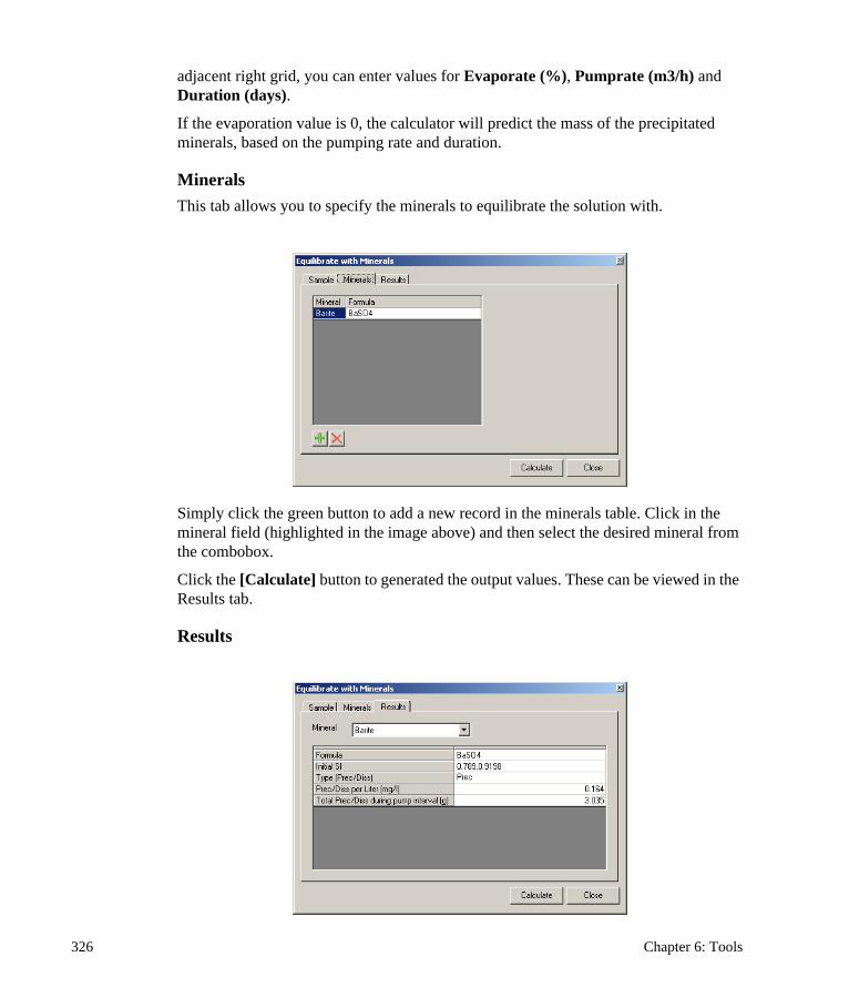
adjacent right grid, you can enter values for Evaporate (%), Pumprate (m3/h) and Duration (days).

If the evaporation value is 0, the calculator will predict the mass of the precipitated minerals, based on the pumping rate and duration.

Minerals This tab allows you to specify the minerals to equilibrate the solution with.

Simply click the green button to add a new record in the minerals table. Click in the mineral field (highlighted in the image above) and then select the desired mineral from the combobox.

Click the [Calculate] button to generated the output values. These can be viewed in the Results tab.

Results

326 Chapter 6: Tools

This tab displays the output results which include the chemistry of the remaining sample as well as the amount of mineral that was precipitated or dissolved (Prec/Diss). If a pumping rate and duration was specified in the Sample tab, the results are also expressed as total prec/diss during the pumping interval.

If you specified multiple minerals in the Mineral tab, you can recalculate the output with respect to different mineral by selecting the mineral from the Mineral combobox and clicking [Calculate].

6.4.5 PHREEQC (Basic)This option loads the PHREEQC (Basic) Input file dialogue as shown below.

This graphical environment facilitates rapid development of simple PHREEQC simulations. Only the basic features of PHREEQC are supported; to take advantage of the more advanced features (Inverse Modeling, Transport, and Kinetics), you may utilize one of the USGS’s PHREEQC versions, as explained below.

AquaChem provides direct access to your AquaChem project database samples for selecting solutions and building the input files. New solutions can be easily defined as needed, or existing solutions from previous simulations can be conveniently selected.

AquaChem also supports the use of flexible units for the various chemicals in solution.

Several simulations can be defined in one input file and processed in a single run. Reactions such as heating, evaporating, dissolving, or precipitating minerals can be conveniently simulated in step wise simulations, with all model parameters calculated for each step.

Once the PHREEQC input files have been prepared, the simulation can be launched directly from AquaChem. When the PHREEQC simulation is completed, you can copy the results from the spreadsheet view, and paste these into the Sample Details window

Modeling 327

for each individual sample. This will allow you to do further processing and analysis, such as plotting, reporting, and querying.

NOTE: Before using PHREEQC, you must ensure that you have defined the location of the PHREEQC.exe (executable), and PHREEQC.dat files. This can be done in the PHREEQC Preferences dialogue, available in the File menu.

For more details on designing a PHREEQC input file, please refer to Chapter 7: Geochemical Modeling with PHREEQC (Basic).

6.4.6 PHREEQC (Advanced)This option allows you to run advanced PHREEQC simulations, using either PHREEQC-Interactive or PHREEQC for Windows. The PHREEQC version that is loaded will be dependent upon the .exe file which is specifed in the Preferences dialogue, as shown below:

In the third line under Files and Folders, you will see a field where you can specify the location of the PHREEQC executable file. If you are using PHREEQC-I, the file is called phreeqci.exe. If you are using PHREEQC for Windows, the file is called phreeqc.exe. Please point this to the appropriate folder on your system where the respective installation resides.

PHREEQC-InteractiveWhen you select the PHREEQC (Advanced) option from the Tools > Modeling menu, this will load the USGS’s PHREEQC- Interactive Windows Interface, provided that this component was successfully installed during your AquaChem installation. An example of the PHREEQC-I window is shown below:

328 Chapter 6: Tools

You may select individual or multiple samples in your active samples list. Any sample(s) which is (are) selected will be used as initial solution(s) when you load the PHREEQC-I program. You may then use the full features that PHREEQC-I has to offer. Once a PHREEQC-I simulation is completed, you must manually insert the results back into AquaChem by copy-and-paste, or by manually typing in the values.

NOTE: Before using PHREEQC-I, you must ensure that you have defined the location of the PHREEQCI.exe (executable). This can be done in the Preferences>PHREEQC dialogue, available in the File menu. If you did not install PHREEQC during your AquaChem installation, you may install this using the installation files located in the PHREEQC folder of your AquaChem CD-ROM. The installation file is named: Phreeqc-2.12.1-669.exe.

For more details on PHREEQC-I, please refer to the user’s manual “manual.pdf” which can be found in the ‘Doc’ folder, in your PHREEQC-I installation directory. Or, you may access the PHREEQC-I On-Line help, from within PHREEQC-I (in the Help menu).

PHREEQC for WindowsPHREEQC for Windows is a 32-bit Windows version of the geochemical model PHREEQC. PHREEQC for Windows contains the full functionality of PHREEQC v.2.

Modeling 329

The input files for the program are backward compatible with the normal version of PHREEQC. This means that you can use any file created with the normal version in PHREEQC for Windows. However, some options that are available in PHREEQC for Windows are not available in the standard version. The PHREEQC for Windows is developed by Vincent E.A. Post.

PHREEQC for Windows is not included with the AquaChem installation. If you would like to install this program, you may use the installation files which can be found on your AquaChem CD-ROM, in the PHREEQC folder. The installation file is named psetup21204.exe. PHREEQC for Windows is a public domain product, and may be downloaded from the web site below:

http://www.geo.vu.nl/users/posv/phreeqc/index.html

Once you have installed PHREEQC for Windows, you must define the location of the PHREEQC.exe (executable), in the PHREEQC Preferences dialogue, available in the File menu. Then, this executable will be launched when you select PHREEQC (Advanced) from the Tools > Modeling menu option.

An example of the input window for PHREEQC for Windows is shown below:

330 Chapter 6: Tools

Similar to the PHREEQC-I, any sample(s) which is (are) selected in your active list will be used as initial solutions when you load the PHREEQC for Windows program. You may select individual or multiple samples in your active samples list. You may then use the full features that PHREEQC for Windows has to offer. Once a simulation is completed, you must manually insert the results back into AquaChem by copy-and-paste, or by manually typing in the values.

For more details on PHREEQC for Windows, please refer to the user’s manual “ManualW.pdf”, which can be found in your PHREEQC for Windows installation folder. Or, you may access the On-Line help, from within PHREEQC for Windows (in the Help menu).

6.4.7 Generate PHT3D Input AquaChem v.5.1 can produce PHT3D input files for use with PHT3D in Visual MODFLOW versions 4.2 or higher.

Visual MODFLOW v.4.2 incorporates the reactive multi-component engine PHT3D. PHT3D couples the transport simulator MT3DMS and the geochemical package PHREEQC-2. Through the flexible, generic nature of PHREEQC-2, PHT3D can handle a broad range of equilibrium and kinetic reactive processes, including aqueous complexation, mineral precipitation/dissolution and (multi-site) ion exchange. In the current version 4.2, Visual MODFLOW data entry is based on the same user interface used for the transport engines such as MT3DMS and RT3D. This has the following drawbacks: typically when using PHT3D, your model will be comprised of many more species than was the case with the former transport engines. Also, PHT3D only accepts special units, and solutions require special conditions such as perfect ion balance, total inorganic carbon entry instead of alkalinity, etc. Therefore laboratory results have to be transformed before the data may be used in PHT3D. To facilitate an efficient workflow, Visual MODFLOW includes an import feature, which allows the user to import solutions, minerals, gas composition and exchanger composition into a selected set of cells. AquaChem, in turn, allows for export of the information stored in its database into the format that can be imported into Visual MODFLOW.

Typically a PHT3D model is comprised of the following elements:

• initial composition of water in the aquifer• composition of inflowing, infiltrating or injected water• properties of the aquifer: mineralogical composition, amount and initial

composition of exchanger places and gas composition

The operations described below are required to transform laboratory results into PHT3D ready input.

Modeling 331

SolutionsAll units must be expressed in mol/l, plus there must be a perfect ion balance between anions and cations. This is achieved by first running a PHREEQC simulation and allowing an automatic charge adjustment, typically on an element which is sufficiently abundant to achieve a balance and which is not considered important for the type of reactions studied through this model. In many cases chloride is a good candidate. Further, PHT3D requires total inorganic carbon as input as opposed to alkalinity which is usually reported in lab results. Again, this requires that the original solution is run and total inorganic carbon is read back from the simulation output file.

MineralsTypically, the laboratory results are provided in ppm or percentage mineral related to 1kg of aquifer material. PHT3D requires the number of mols of mineral related to the mass of aquifer material in contact with 1 liter of pore water. This requires knowledge about the porosity and density of the aquifer material. For example, an aquifer having porosity of 20% and density of 2.7 g/cm3 will have a volume of 4 liter of rock around every liter of pore water resulting in a mass of 10.8 kg of rock material. If this rock comprises 10% of calcite, the mols of calcite is calculated as 10.8 * 0.1 * FMW(calcite, 0.1 kg) 10.08 mols. This calculation needs to be repeated for each mineral.

ExchangersPHT3D requires the amount of exchange places and the initial occupation of these places with various available ions, e.g. NaX, CaX2, MgX2, KX, etc. As in the previous case, the concentrations refer to 1 liter of pore water, though in reality, these values are rarely available. Values provided by the laboratory normally include the CEC (cation exchange capacity, which may be transformed into exchange places per liter of pore water in a similar way as discussed for the minerals. More often, the CEC itself has to be estimated based on the amount and type of clay minerals and presence of organic material. A formula that is often applied in this respect is given by Appelo and Postma, 1993:

CEC = 3.7 * %clay + 3.5 * % organic C

If the type of the dominant clay material is known, then the CEC can also be estimated by multiplying the average CEC of this clay material with the percentage reported in the studied aquifer material.

All above methods only provide the places available for ion exchange, but do not indicate the initial occupation of these places. If an exchanger material assumed to be in equilibrium with a given solution, e.g. fresh water or sea water, then PHREEQC allows calculating this initial composition using the so-called implicit option for the exchange simulation. As for the solution, the PHREEQC output can then be used as input for PHT3D.

332 Chapter 6: Tools

Create Input FilesFor models comprised of many species, data entry and associated conversion and transformation may turn out to be very tedious. AquaChem, therefore, includes an option to facilitate this data entry as explained below.

Requirements:

• A VMOD project must exist, since AquaChem reads information from the *.vmf file.

• A VMOD installation must exist on the local computer or network, since AquaChem needs to have access to the vmod.xml file in order to find the thermodynamic database.

To create a PHT3D input file:

Generate PHT3D Input from the Tools > Modeling menu, and the screen depicted in figure below will appear.

Each tab is described in detail below:

General TabThe VMOD Program Folder field allows you to select the VMOD installation folder (where the vmod.xml file is located).

Click the button beside the VMOD Program Folder field, in the top right corner and navigate to the VMOD installation folder. Select the folder and click [OK].

Modeling 333

The VMOD Project field allows the user to specify the folders where the project .VMF file is located. AquaChem reads all required information from the XML file and displays it in the grid.

Click the button beside the VMOD project field and navigate to the VMOD installation folder. Select the file and click [OK].

The remaining tabs, i.e., solution, aquifer and preview, provide an interface to define the composition that will be importable in PHT3D (solutions, minerals, gas composition, exchanger composition).

The first tab allows you to format the entry for one or several solutions. The solutions must have been previously entered in AquaChem using standard units. Another important precondition for assigning AquaChem concentrations to PHREEQC master species is that the master species are matched to AquaChem database parameters in the currently active thermodynamic database.

Solutions tabThe Solutions tab allows converting AquaChem solutions into PHT3D importable solutions including charge balance calculations and conversions to mol/L. When this tab is displayed, the grid below is shown. It lists all master species of the current thermodynamic database for the active VMOD project variant. The active compounds are marked in the third column by the internal concentration name, i.e., conc0001, conc0002, etc.

334 Chapter 6: Tools

Click the [Select] button to open the Station List dialog (shown below).

Select a sample from the station list, and click the [Assign] button and then [Close].

All available concentrations from the selected sample will be copied to the “Conc” column in their original format.

The Charge Balance combo box allows you to select an element that will be used for calculating the charge balance. Please note that only the active PHT3D components will be used for the PHREEQC simulation. Therefore an AquaChem sample, that is perfectly balanced, but includes species which are not active in PHT3D, still needs to be balanced.

All available active PHT3D species will be written to a PHREEQC input file and the charge balance is calculated as well as redox species, e.g., Fe(2), Fe(3) from total Fe. All results are read back in mols/L column in the grid immediately (shown below). You may edit the concentration column manually however you will need to click the [Run] button to launch the PHREEQC simulation manually. When changing the element used to calculate the ion balance, the simulation is launched automatically.

Modeling 335

Use the format combo box to specify the appropriate format for the generated input file. You can choose from initial concentration or recharge concentration.

For more information on recharge concentration format, see “Preview Tab” on page 340

Aquifer tabThe Aquifer tab allows you to define the mineral composition of the aquifer. Note that PHT3D uses concentrations per liter of bulk aquifer material rather than per liter of porewater used by PHREEQC.

First, define the bulk density by entering the value in the Bulk Density text field. This value can be calculated based on the porosity and the density of grains. Most rock forming minerals have a density of 2.6-2.75 g/cc. Porosity can vary more widely from a few percent up to 60% for clays.

Click the button to access the AquaChem bulk density calculator (shown below).

336 Chapter 6: Tools

Enter a Porosity and Density value and then click the [Calculate] button to generate the Bulk Density value. Click [Close] and enter the generated value into the Bulk Density text field in the Aquifer tab.

MineralsIn the Phase Assembly (Minerals) frame, enter the estimated or measured percentages for each listed mineral in the % column. The respective mols/L of aquifer bulk material will be calculated in the last column (shown below).

Exchanger SitesThe definition of an exchanger assemblage requires two basic inputs: the amount of total available sites and the initial distribution of these sites among the active PHT3D exchanger components. Because these values are not always directly measured, you can use the AquaChem calculator to generate estimated values.

The first step of calculating an exchanger composition consists of estimating the amount of exchanger sites in the aquifer material that is in contact with 1 liter for pore-water. Click the button and the screen shown below will be shown.

Modeling 337

Under the General tab, calculate the Bulk Density by entering grain density and porosity values or simply enter the bulk density if the value is already known.

Next click on the Exchange Capacity tab.

For this example the exchange places are to be estimated based on a known percentage of 10% clay and 5% organic matter. Enter these percentage values in the first two text boxes. Click the CEC estimated radio button. Once the [Calculate] button is clicked, the CEC in meq/100g soil will be calculated and multiplied by the mass of grains calculated on the first tab.

Copy the calculated value to the clipboard (highlight value, right-click and select copy) and then paste the value into the Exchanger sites field of the Minerals tab.

There are two ways of entering the distribution of sites among Exchanger species: Explicit requires that you distribute the sites manually among the species, based on laboratory results or estimation. The Implicit method allows selecting a solution,

338 Chapter 6: Tools

equilibrates the exchanger assemblage with this solution, and then reads the results back to the grid. Both methods are described in more detail in the following sections.

ExplicitIf the distribution of specific exchange places (CaX2, NaX, KX, etc.) is known, enter the percent values manually in the grid below for each exchanger.

Implicit Alternatively you may assume that the exchanger is in equilibrium with a solution. Typically for exchange reaction simulations, the aquifer including its exchangers is in equilibrium with an initial solution. This system is then flushed with a solution of a different composition (e.g. saltwater if the initial solution was freshwater or vice versa). The first solution can be used to calculate the distribution of individual exchange species (CaX2, NaX, KX, etc.).

Select the Implicit option, then press the button and select the required sample from the Station List dialog (shown below).

Once selected, click the [Assign] button.

This will automatically generate a PHREEQC simulation, equilibrating an exchanger having the specified number of exchange places with this solution. The calculated

Modeling 339

exchange species are then extracted from the PHREEQC output file and inserted into the grid.

Preview TabThe preview tab provides a summary of the prepared data for PHT3D import. Three different entries are created: initial concentration, mineral composition and exchanger composition. Each grid contains a [Save] button which allows you to export the grid data to an importable text file (indicated in the image below).

Exchanger and mineral composition can only be defined under the initial concentrations format. The respective datafiles are time independent. Solutions may also be bound to time dependant boundary conditions such as recharge and point sources. Among those, only the creation of recharge concentrations is supported for the time being.

To create recharge concentrations, simply select Recharge concentrations from the Format combo box in the General tab.

340 Chapter 6: Tools

The preview grid for solutions will now be filled with multiple records (shown below). The number of time steps and the simulation duration is read directly from the project.vmf file and is also displayed in the project setting grid on the General tab. For the time being, the composition of every step is kept constant. This grid is editable; you may add or delete rows and change the start/stop values for every row. For example, if the solution includes a parameter for temperature, you can manually change this value for every time step, while the composition of the water remains constant.

Once the grid data has been saved in imported text files, they can be imported into VMOD/PHT3D.

Modeling 341

342 Chapter 6: Tools

7Geochemical Modeling with PHREEQC (Basic)

This chapter presents an overview of the modeling capabilities of PHREEQC and an introduction on how to create PHREEQC Input files using the basic version of PHREEQC included within the AquaChem interface.

Here you will find an introduction to the AquaChem Interface to PHREEQC, PHREEQC Window Layout, Creating PHREEQC Input Files, and Running PHREEQC Simulation.

AquaChem uses the batch version of PHREEQC, which allows to integrate this model seamlessly into AquaChem. For details on the Graphical User Interfaces PHREEQC-I, or PHREEQC for Windows, please refer to the User’s Manuals included with these programs. Or, for a basic description, please refer to PHREEQC (Basic) section in Chapter 6.

7.1 AquaChem Interface to PHREEQCPHREEQC is a computer program for speciation, batch-reaction, one-dimensional transport, inverse geochemical calculations, and much more. For more than twenty years, the USGS’s PHREEQC has been the proven standard for aqueous geochemical modeling. PHREEQC is derived from the FORTRAN program PHREEQE. As the name implies, the original FORTRAN code has been entirely rewritten in the C programming language and this new version has eliminated many of the deficiencies and limitations of earlier version of PHREEQE, while adding many new powerful analytical capabilities.

In the past years the authors of PHREEQC have not only added many more powerful features to the program, but they have also implemented two very easy-to-use interfaces for writing input files and analyzing output files for the PHREEQC program. The respective programs PHREEQC-I and PHREEQC for Windows are included with your AquaChem installation CD; you may link your AquaChem samples in your database to either one of these programs, provided that these programs are installed, and linked in the File > Preferences dialogue. These interfaces may be called from

AquaChem Interface to PHREEQC 343

within AquaChem, and this will allow you to run advanced PHREEQC simulations using your AquaChem samples. For more details, please refer to Chapter 6.

The PHREEQC (Basic) option provides a GUI to the basic features of PHREEQC. You may run simple simulations based on analysis stored in the AquaChem database; this option also allows you to create PHREEQC input files, can be later opened with more sophisticated graphical user interfaces such as PHREEQCI or PHREEQC for Windows versions of PHREEQC.

Although this chapter describes how to create PHREEQC input files with the PHREEQC (Basic) version, the concept of hydrochemical modeling and the PHREEQC program will not be discussed in detail. It is recommended that you read the PHREEQC user’s manual before performing any complex hydrochemical simulations. For your reference, the PHREEQC user’s manual and source code may be downloaded from the following web site: http://wwwbrr.cr.usgs.gov/projects/GWC_coupled/phreeqc/. In addition, the PHREEQC user’s manual is available on the AquaChem installation CD-ROM, and in your AquaChem installation folder.

7.1.1 Preferences for PHREEQCThe instructions in this chapter will be based on the assumption that you are using the PHREEQC executable file (PHREEQC.exe - PHREEQC version 2.8) included with AquaChem. By default, the PHREEQC batch executable file and the PHREEQC thermodynamic database files are automatically installed in the default folder, C:\Program Files\AquaChem. If you have installed AquaChem in a directory other than the default installation directory, or if aquachem is not yet linked to PHREEQC, the Tools/Modeling/PHREEQC (Advanced) option will be inactive (greyed out) on your computer, and you will need to manually set up the link between AquaChem and the PHREEQC thermodynamic database and executable files.

To do so, select File from the main menu and then select Preferences. The following Preferences dialogue will appear. In this dialogue, select the PHREEQC tab.

Under the Files and Folders frame, press button beside the Thermodynamic Database field and select the path and filename from the PHREEQC Thermodynamic Database dialogue. From this dialogue, select either phreeqc.dat, Wateq4f.dat or

344 Chapter 7: GeoChemical Modeling with PHREEQC

Minteq.dat. In addition, in the PHREEQC Executable field select the path and filename for the phreeqc.exe file. Finally, specify the path and filename for the USGS PHREEQC Executable file (which is used in the PHREEQC (Advanced) option).

If the default path and filename are incorrect, you can browse the directory by clicking

on the button and select the filename.

By default, all PHREEQC input and output files will be saved in your AquaChem installation folder (default is C:\Program Files\AquaChem).

Once you are finished, click [Save] then [Close]. You are now ready to run PHREEQC.

7.1.2 The PHREEQC Thermodynamic Database LinkOne of the biggest advantages of the AquaChem PHREEQC interface is the direct link between the two databases of these programs. The link allows you to use samples from the AquaChem database and read them into the PHREEQC input data file.

In order to let AquaChem know which database parameter matches which PHREEQC element, some minor modifications have been made to each of the thermodynamic databases included with AquaChem. The link between AquaChem and the thermodynamic databases is established by adding the AquaChem parameter name as a comment for each matching parameter in the Masterspecies section of the database file. Each comment is preceded by a ‘#’ character to flag the AquaChem parameter descriptor.

For example, the following lines are taken from the Masterspecies section of the phreeqc.dat file:

These modifications have already been defined for each of the thermodynamic database files provided with AquaChem. You have to redefine this only if you change the thermodynamic database.

Ca Ca+2 0.0 Ca 40.08 #CA

Mg Mg+2 0.0 Mg 24.312 #MG

Na Na+ 0.0 Na 22.9898 #NA

K K+ 0.0 K 39.102 #K

Fe Fe+2 0.0 Fe 55.847 #FE

Fe(+2) Fe+2 0.0 Fe

Fe(+3) Fe+3 -2.0 Fe

Mn Mn+2 0.0 Mn 54.938 #MN

AquaChem Interface to PHREEQC 345

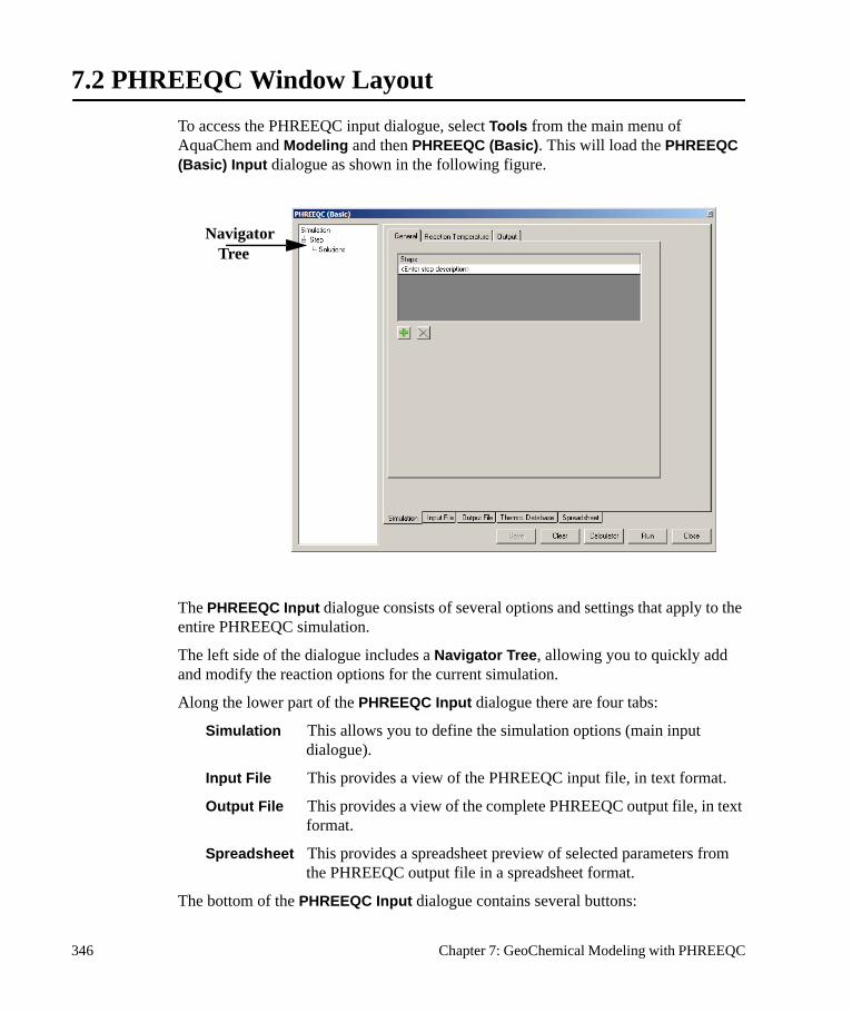
7.2 PHREEQC Window Layout To access the PHREEQC input dialogue, select Tools from the main menu of AquaChem and Modeling and then PHREEQC (Basic). This will load the PHREEQC (Basic) Input dialogue as shown in the following figure.

The PHREEQC Input dialogue consists of several options and settings that apply to the entire PHREEQC simulation.

The left side of the dialogue includes a Navigator Tree, allowing you to quickly add and modify the reaction options for the current simulation.

Along the lower part of the PHREEQC Input dialogue there are four tabs:

Simulation This allows you to define the simulation options (main input dialogue).

Input File This provides a view of the PHREEQC input file, in text format.

Output File This provides a view of the complete PHREEQC output file, in text format.

Spreadsheet This provides a spreadsheet preview of selected parameters from the PHREEQC output file in a spreadsheet format.

The bottom of the PHREEQC Input dialogue contains several buttons:

Navigator Tree

346 Chapter 7: GeoChemical Modeling with PHREEQC

The save button allows you to save the contents of the input or output file. If the Input File tab is selected, the [Save] button will allow you to save the input file as a .PQI file. If desired, this file may be loaded into

PHREEQC-I, and the simulation may be run using this version. If the Output File tab is selected, the Save button will allow you to save the output file as a .PQO file.

The [Clear] button clears the contents of the input file, and allows you to create a clean, new input file.

The [Calculator] button loads the Aquifer Properties Conversion dialogue and allows you to calculate and convert various aquifer properties you require for some of the PHREEQC simulations.

The [Run] button runs PHREEQC using the current simulation options. This button loads the PHREEQC input file and executes the PHREEQC simulation. The [Run] button should only be used after you have

specified all of the required run options and you are ready to start the PHREEQC simulation. It is recommended that you verify the input file before running the simulation.

The [Close] button closes the PHREEQC input dialogue.

There are four tabs associated with the [Calculator] button: General, Surface Complexation, Exchange Capacity, and Mineral Assemblage. These are shown and described below:

GeneralSince PHREEQC always assumes a solution volume of 1.0 liters, the General calculator allows you to easily calculate the Volume of rock (liters) per liter of porewater and Mass of grains (kg) per liter of porewater for the aquifer based on a solution containing 1.0 liters of porewater. Simply enter the input parameters

PHREEQC Window Layout 347

(Porosity, Density), and press the [Calculate] button. This provides the necessary values for all calculations shown below.

Surface ComplexationThe moles of surface places (sites) depends on the content of hydrous ferric oxides in the aquifer (Sites/mol ferrous iron). Fe is generally a measured parameter but you must estimate the percentage of iron (Weight % Fe) that is in the form of hydrous iron (% hydrous ferric oxides of total iron). Since PHREEQC always asks for mols, you also need a formula weight value for your iron minerals. Hydrous iron is a mixture of several minerals, so a suggested Gram formula weight for oxides is 89 which is used as a default value.

Exchange CapacityThe Cation Exchange Capacity (CEC) is normally expressed as meq/100g of soil. PHREEQC however uses meq/l of porewater. There are several ways of estimating the number of exchangeable sites and express it in the unit used by PHREEQC.

If you know the CEC value you may directly enter it and calculate the exchange places (Sites) within the given aquifer volume. Otherwise you need to estimate the CEC. The first option lets you select a clay mineral from a list and will use an average CEC value. Choose this option if you know the dominant clay mineral of your aquifer. If you know only the percentage but not the mineralogy of your clay minerals you may use a formula derived by Appelo (1993) to estimate the CEC:

CEC=0.7 * clay% +3.5 * org material%.

348 Chapter 7: GeoChemical Modeling with PHREEQC

Mineral AssemblageThe Mineral Assemblage option lets you convert an analysis usually expressed as weight percent to mol of mineral per liter of porewater. Simply select a mineral from the combo box, and specify a Weight %. Press [Calculate] and the amount of mols will be calculated.

There are three tabs associated with the Simulation tab which are shown and described below:

GeneralThe General tab contains a summary of the steps defined for the current simulation.

PHREEQC Window Layout 349

Reaction TemperatureThis tab provides options to specify the reaction temperature, or step-wise changes in the reaction temperature. The Reaction Temperature options can be seen in the dialogue shown below.

The Reaction Temperature tab provides options for specifying the desired temperature settings during a modeled reaction. Normally the temperature of the selected sample stays Constant (default setting) during a reaction and it will use the solution temperature as entered in the Solutions option selected from Navigator tree. However, PHREEQC provides you the options to change the temperature linearly (Linear change from...to...in...Steps) from a starting temperature to an ending temperature in a specified number of steps or in steps during the course of a simulation. The List of Steps option allows you to specify the exact temperature at specific steps during the reaction and the temperatures will be applied in the order they are listed.

OutputThe Output tab allows you to access the various output details to include in the standard PHREEQC results output file (.PQO file extension) or to save simulations directly back to the database. PHREEQC will generate an output file every time you run a simulation. However, this file is very detailed and may contain more information than you need to solve a particular problem. Its format is also not suited for plotting or presenting simulated data. This tab lets you extract individual parameters from the detailed output file and write them into a spreadsheet.

The options available under the Selected Output dialogue are shown in the figure below:

350 Chapter 7: GeoChemical Modeling with PHREEQC

Selected Output

With the selected output option, you may extract specified activities, saturation indices, gas phases, etc. into a spreadsheet type file.

Simply choose the parameters you want to save to the tabular output file. By default the parameters pH, pe, Temperature and Ionic Strength are included in the output.

Totals Total amount of a masterspecies, this value should be equal to the entered concentrations

Activities Amount of aqueous species that is available for reactions.

Molalities Concentrations of aqueous species

Saturation indices Saturation state of minerals

Equilibrium phases:Amount of minerals present in the system

Gas phases: Amount of gas phases present in the system

When you have successfully run the simulation, AquaChem allows you to save the

output file. To do so, press the button, and enter a filename.

PHREEQC Window Layout 351

Prepare simulated output for storage in database

If the database is selected as the target output, then the simulated results for created samples will be saved as new sample records. This option is only applicable if a simulation creates a new solution, e.g. when mixing several existing samples, when equilibrating an existing sample with minerals, or when adding chemicals. Since every sample needs to have an assigned station, you should create one or several dummy simulation stations, to which you may assign your simulated samples in order to easily distinguish them from real samples. If the sample comment field exists and is identified and mapped in the File>Database>Aliases section, then the type of simulation will be written automatically to the sample.

Simulated samples do not necessarily belong to a station, e.g. when saving the mixture between 2 samples, the saved simulated composition would belong to no specific station. However, AquaChem needs a station to be assigned to every sample, therefore the Save simulated solution output to database option requires you to define the station for the new samples to be created. You may create a dummy station names, such as “PHREEQC Simulation” that may be used for this purpose.

Save OptionsThe PHREEQC input and output files are saved by Aquachem under default filenames which will be overwritten with every new PHREEQC run. Using the “Save Solution as” option in the step frames, allows you to save the current simulation under a defined name. You may afterwards use this file for your documentation or continue to model with one of the USGS GUIs that provide more advanced coverage of the PHREEQC features.

7.3 Creating PHREEQC Input Files

7.3.1 Simulation - StepsA PHREEQC simulation may consist of several steps (e.g you may define and mix 2 samples in the first step and equilibrate the mixing result in a second step).

Under the General tab, you will see a list of Steps (if multiple steps have been defined).

In order to add a simulation step you may right click on Simulation - the top item of the

Navigation tree - and select the Add Step. Or click the button below the Steps frame.

352 Chapter 7: GeoChemical Modeling with PHREEQC

You can enter a name for the Step in the Description field, and choose the step properties. Click button under the Add and choose an item from the list, and press

the button.

After a new step has been added, double click on it or click on the Step in the Navigator tree to produce the Step description dialogue:

This new item will now appear in the Navigator tree on the left side of your display. To activate the properties for this item, expand the Navigator tree and click once on this item.

To modify the Step properties, you have two options:

[1] Double click on the Step name from the main dialogue, OR[2] Select “Step” from the Navigator tree on the left side of your display.

Options for the reaction steps can also be created and modified as needed. These include:

• Add Initial Conditions and• Forward Modeling

These options are described in detail in the following sections.

Creating PHREEQC Input Files 353

Add Initial ConditionsAdd Equilibrium Phases

Add Exchange Assemblage

Add Gas Phase Assemblage

Add Solutions

Add Surface Assemblage

Forward ModelingAdd Mix Solutions

Add Reactions

7.3.2 Equilibrium PhasesAdding Equilibrium mineral phases is similar to adding reactions. With the Add Reaction options (described below) you add a specified amount of a phase, but with the Add Equilibrium Phase options the amount of mineral phase added is limited by a specified saturation index.

To specify an equilibration of your solution with Mineral Phases, right click on the Steps options and select Add Initial Conditions from the pop-up menu and then select Add Equilibrium Phases.

354 Chapter 7: GeoChemical Modeling with PHREEQC

Equilibrium Assemblage

Each mineral phase assemblage is identified by a unique Phase assemblage Number and a Description. You may enter multiple phases by specifying a phase number from # to # (ex. Number 1 to 2). The assemblage number is only important if you intend to use the input file later for transport modeling using PHREEQCI or PHREEQC for Windows.

• Select Equilibrium Phases1 and an Equilibrium Phases dialogue will appear as shown below.

For each mineral phase you choose, you can specify the following properties:

SI: This is the Saturation Index of the selected mineral phase (degree of saturation, default value 0).

SI = log(IAP/KT)

where,

IAP = the ion activity product for the given material and

KT = the reaction constant at the given temperature

If SI > 0, then the solution is super-saturated with respect to the mineral phase;

Creating PHREEQC Input Files 355

If SI < 0, then the solution is below saturation of the specified mineral phase.

If SI = 0, then the solution is in equilibrium with the specified mineral phase.

For Gas phases the SI corresponds to the log of the partial pressure.

Mols: Mols describes the maximum amount of mineral phase that can be added or dissolved to reach the specified saturation. The default value is 10 mols. The constraint on available amount of mols is important if you want to translate measured concentrations of minerals in an aquifer in a PHREEQC transport model. You may also set the amount of available mols to 0, making sure that the respective mineral can only be precipitated but not dissolved from the aquifer.

Alternative phase: The alternative phase is added or removed until the first mineral is in equilibrium with specified saturation index. For example, gypsum may be added or removed to the solution until an equilibrium with the primary mineral calcite is reached. An amount must be specified for the alternative mineral phase (default amount of the alternative phase is 10 moles as specified by PHREEQC). The solutions equilibration with calcite will be terminated if the amount specified for the alternative mineral phase is consumed prior to equilibration with calcite. It should be noted that if the alternative phase is specified, the amount of the mineral phase is ignored. Otherwise the system would be overdetermined.

Below the grid, select the solution with which the mineral phase will be equilibrated. If you do not choose a solution, the specified assemblage is equilibrated with the first solution defined in the current simulation.

The equilibration of a solution with minerals will result in a new composition of the solution. The Save Solution as allows you to save this composition as a new solution. These new ‘elements’ can then be used as input data for subsequent PHREEQC simulations. Each of these new elements must be identified by a unique number that is not already in use. If you specify a number that is currently in use, the new element will overwrite the old element.

7.3.3 Exchange Assemblage Ion exchange involves the replacement of one chemical in the solution with another on a solid surface. Intrusion of fresh water into marine sediments or seawater into coastal fresh water aquifers are probably the best known examples for this mechanism. Fresh water typically is dominated by Ca2+ and HCO3

- ions due to the presence of dissolved calcite, whereas in seawater, Na+ and Cl- are the dominant ions. Sediment in contact with sea water will often have large concentrations of Na+.

356 Chapter 7: GeoChemical Modeling with PHREEQC

When seawater intrudes in a coastal fresh water aquifer an exchange of cations takes place:

2Na+ + Ca-X2 --> (2Na-X + Ca2+)

where X indicates the soil exchanger.

Sodium is taken up by the exchanger and Ca2+ is then released. The composition of the solution and the exchanger is modified by this reaction.

A sample of the Exchange Assemblage options dialogue is seen below:

PHREEQC lets you define the initial composition of an Exchange Assemblage in two ways:

[1] Explicitly by selecting the composition of the Exchange Assemblage. This approach is chosen if the mineralogy and the exchange sites for these minerals are well known.

[2] Implicitly by specifying that the Exchange Assemblage is in equilibrium with a solution of a fixed composition. This approach is chosen if the type of water in the aquifer is known. E.g. to model an aquifer in contact with seawater make sure that your model contains a seawater sample and specify this sample within the “Exchange assemblage is defined to e in equilibrium with solution” option.

Creating PHREEQC Input Files 357

Option 1

AquaChem provides a list of available exchanger ions to choose from and allows you to easily add several ions to the Exchange Assemblage.

To add an ion(s) to the Exchange Assemblage:

• Click to add a new line to the grid. • Under the Exchanger field, double-click in the first empty cell and a combo

box with a button will appear listing the available items. • Select the ion you need, and press <Enter> (on your keyboard). The ion will

appear in the grid. • Enter the Amount (in Mols) for each ion in the Exchanger column. In order to

estimate the amount of exchangeable cations, you may use the Aquifer Properties Calculator described above.

To remove an ion from the Exchange Assemblage, click-on the ion you would like to remove, and then press the button.

Option 2

You may specify that the Exchange assemblage is defined to be in equilibrium with a solution. For example, if you consider that the exchange takes place on a marine clay, define seawater as a solution and select this solution in the Implicit option as the water the exchange material is in equilibrium with. Simply enter a solution number in the appropriate field.

Once you have defined the Exchange Assemblage, you must select the solution with which you wish to equilibrate. If you do not select a solution from the list, you can save the Exchange Assemblage to equilibrate in a later simulation step (e.g. during a transport problem).

Each Exchange Assemblage is identified by a unique Number and a Description so they can be easily recognized in the Input / Output files, and reused in later simulations.

The Save Solution as field allows you to save the composition of a simulation by creating a new exchange assemblage. These new ‘elements’ can then be used as input data for subsequent PHREEQC simulations. Each of these new elements must be identified by a unique number that is not already in use. If you specify a number that is currently in use, the new element will overwrite the old element.

7.3.4 Gas Phase AssemblageThe Gas Phase is used to equilibrate a solution with a finite volume of gas. This simulation is not applicable if fixed partial pressures of the gas components are desired (for this case use the Mineral Phase option instead and fix a gas with a partial pressure

358 Chapter 7: GeoChemical Modeling with PHREEQC

that has an infinite volume of gas phase). An example of the Gas Phase Assemblage dialogue is shown below:

The Gas Phase option will equlibriate the solution with only those gases which are defined in the simulation. However, gases may be specified with a partial pressure equal to zero at the start of the simulation. In this case, no moles of that component will be present initially, but some gases may evolve during a reaction simulation such as oxidation of organic material. As a result, the partial pressure of all gases included in the gas phase stays constant and the excess gas is removed from the solution as the gas bubbles.

Pressure calculations are computed using the ideal gas law,

PV = nRT

where,

P = defined pressure

V = volume

n = number of moles of the gas

R = universal gas constant

T = temperature

Creating PHREEQC Input Files 359

AquaChem provides a list of available gases to choose from and allows you to easily add multiple gases to the Gas Phase Assemblage.

To add a gas phase assemblage to the simulation:

• Click to add a new line to the grid.• Under the Gas Phase field, double-click in the first empty cell and a combo

box with a button will appear listing the available items. • Select the gas you need, and press <Enter> (on your keyboard). The gas will

appear in the grid. • Enter a partial pressure value for each gas under the Part. Press column.

If you wish to add air to the solution, click on button and the major components of air will be automatically added to the list, with their partial pressures at 1 bar.

To remove a gas from the Gas Phase Assemblage table, select the gas to remove and then press the button.

The Critical Pressure, Initial Volume and Temperature information is required for each Gas Phase assemblage in order to calculate the weights of each gas component.

The default values are:

Critical Pressure: 1.1 atm. This is equal to the pressure, at which the dissolved gas will start to create bubbles

Initial Volume: 1.0 liters: amount of gas initially in the system

Temperature: 25°C

Finally, you can select the solution with which you would like to equilibrate the gas phase assemblage. If you do not select a solution from the list, you can save the gas phase to equilibrate in a later simulation step. Each Gas Phase Assemblage is identified by a unique number and can be reused in later simulations.

The Save Solution as allows you to save the composition of a simulation by creating a new gas phase assemblage. These new ‘elements’ can then be used as input data for subsequent PHREEQC simulations. Each of these new elements must be identified by a

360 Chapter 7: GeoChemical Modeling with PHREEQC

unique number that is not already in use. If you specify a number that is currently in use, the new element will overwrite the old element.

7.3.5 Adding SolutionsIn PHREEQC, a "solution" is a set of analyses for a single water sample. AquaChem automatically creates a PHREEQC input file from the sample details pertaining to your AquaChem database, or from a pure water sample.

To access the solutions options, expand the items in the Navigator tree by pressing the + beside Step. Then select Solutions and the solutions frame should appear, similar to the one below.

You must specify at least one solution for every PHREEQC simulation file. AquaChem allows you to select from two types of solutions:

• Samples from your AquaChem database; OR• Pure Water

These options are described in detail in the following sections.

Creating PHREEQC Input Files 361

Using Samples from your AquaChem DatabaseTo add a sample from your database as a solution, select the sample from the list at the top, and press the button. The sample will then be added to the Solutions frame in the lower half of the dialogue; in addition, the new solution will show up as a new line in the Navigation tree, under Solutions.

To add multiple samples from your database, use the <Shift> and <Ctrl> keys with the mouse to select the samples you need, then click the button. This is useful if you want to speciate a large number of samples simultaneously. Each complete sample should have pH, alkalinity, and temperature values specified.

The AquaChem database index Number for the selected sample will be used as the Solution number. The Description field is used to identify the solutions. The solution description will appear in the PHREEQC input file.

After you have added a solution, you can verify that it has been added to the PHREEQC input file. To do so, click the Input File tab at the bottom of the screen and you should see the added solution and any corresponding concentrations.

Adding Pure Water

To add pure water as a solution, press the button below the list of AquaChem active solutions. For certain simulations it might be useful to have pure water as a base solution. For example, you can simulate a groundwater by saturating pure water with calcite and adding a specified CO2 pressure.

Solution PropertiesOnce you have added a solution, you may want to modify the Solution properties.

To do so, you have two options:

• In the Solutions frame, double click on the appropriate solution from the main dialogue, OR

• Select the appropriate Solution #, from the Navigator tree on the left side of your display.

362 Chapter 7: GeoChemical Modeling with PHREEQC

The Solutions properties frame should appear as shown below.

The upper part of this dialogue lists the solution Description and Number. As discussed above, the Number is AquaChem database index number for the selected sample which will be used as the Solution number. The Description field is used to identify the solutions.

The remaining options in this frame are separated into two tabs:

• General, and • Concentrations

The options associated with these tabs are described in detail in the following section.

GeneralUnder the General tab, you can specify options for pH and Redox during the simulation.

Creating PHREEQC Input Files 363

You can choose a Constant during reaction value for these parameters, or allow the values to be determined as a result of equilibration with a mineral phase (Determined by equilibration with phase).

In addition, at the bottom of the frame, you can enter a default Temperature and Density values for the solution. The sample density is only needed when concentration values are entered in ppm or ppb.

ConcentrationsThis tab lists the concentrations of the dissolved elements in solution.

The first column of the grid contains the Element name, while the second column describes the PHREEQC Masterspecies (M. Spec.) name.

The parameter values are read from the database; if necessary you may add or remove concentrations (Conc.), or edit the existing values. You may also define a concentration as controlled by a mineral solubility, or for gases, by a defined pressure. For example, a calcium concentration is overridden in the simulation by a calculated value that will result in a calcite equilibrium state (Saturation index = 0).

Once you have entered element values for the pure water solution, the Default Unit may not be changed. However, you can change the unit individually for each entered

364 Chapter 7: GeoChemical Modeling with PHREEQC

value by clicking button in the Unit column. Please note that it is not possible to freely mix units (i.e. you may not enter some values as mg/L and others as mmol/l). You may only mix units within a "unit family" such as g/L, mg/L ug/L.

Example

The following example will demonstrate how to use a sample from the Demo database, as a solution in a PHREEQC simulation:

To add the MW-1-92 sample from the DEMO.AQC database to a PHREEQC input file, proceed as follows:

• Tools from the main menu, then select Modeling and then PHREEQC (Basic) from the main menu.

• Click + beside Step (in the Navigator tree) and you will see Solutions• Select Solutions• Select the MW-1-92 sample (ID = 1) at the top of the list of Active solutions

in database frame• Click button and the sample will now appear in the Solutions frame in the

bottom section of the dialogue.

To view the solution properties, double click on this Solutions, or expand the Navigator tree, and select the Solution from here. This will load a Solution properties dialogue.

Click on the Concentrations tab to confirm that the concentrations are identical to those entered for that sample in the AquaChem database.

To verify that this data is saved to the PHREEQC input file, you can view the input file by clicking the Input File tab at the bottom of the dialogue.

7.3.6 Surface AssemblageWhile ions are exchanged during an exchange process, surface processes involve only the absorption of material on mineral surfaces. This process typically can be observed on hydroxides and is driven by electrostatic processes.

An example of the Surface options dialogue is seen below:

Creating PHREEQC Input Files 365

PHREEQC lets you define the initial composition of a Surface Assemblage in two ways:

1. Explicitly by specifying the parameter values for Surface Assemblage; or

2. Implicitly by specifying that the Surface Assemblage is in equilibrium with a solution of a fixed composition.

Option 1 (Explicit)

To define a Surface Assemblage:

• Click to add a new line to the grid.• Under the Binding Site field, double-click in the first empty cell and a combo

box with a button will appear listing the available items. • Select a Binding site, and press <Enter> (on your keyboard). • Overwrite the default values for Specific Area (600 m2) and Weight (89 g) if

required. Weight is defined as mass of solid for calculation of surface area in grams. Surface area is mass times specific area per gram.

• Specify the total number of Sites (in mols) for each binding and make any appropriate changes to the default values for Specific Area and Weight.

366 Chapter 7: GeoChemical Modeling with PHREEQC

• Choose the appropriate diffuse layer model for the surface reaction (please see the PHREEQC manual for information on selecting the appropriate Diffuse Layer Options for your surface reactions).

To remove a binding site from the Surface Assemblage, select the Binding Site you would like to remove and press the button.

Option 2 (Implicit)

You may specify that the Surface Assemblage is defined to be in equilibrium with a solution. Simply enter a solution number in the appropriate field.

Once you have defined the Surface Assemblage, you must select the solution with which you wish to equilibrate. Each Surface Assemblage is identified by a unique Number and a Description so they can be easily recognized and reused in later simulations.

The Save Solution as allows you to save the composition of a simulation by creating a new surface assemblage. These new ‘elements’ can then be used as input data for subsequent PHREEQC simulations. Each of these new elements must be identified by a unique number that is not already in use. If you specify a number that is currently in use, the new element will overwrite the old element.

7.3.7 Mix SolutionsThe Mix Solutions allows you to simulate the mixing of multiple solutions together with different proportions of each solution added to the mixture. An example of the Mix options dialogue is seen below:

Creating PHREEQC Input Files 367

To simulate mixing multiple samples together, you must first specify at least two solutions for the PHREEQC simulation.

To add a solution to the mixture:

• Click to add a new line to the grid under the Solution header. • Type in a Solution number in the same cell. • Click-on the first line in the grid under the Part header and type the proportion

of the solution you would like to add to the mixture (e.g. 3 parts of Solution 1 and 4 parts of Solution 2)

The solutions will be automatically added to the input file. Note that if you want to simulate several mixing proportions between two samples, each mix must be conducted in a separate simulation step as otherwise only the first mix definition will be executed.

Each mixed solution has a unique Mix number and Description. To re-use the simulated mixed sample in a later step, simply enter a solution number beside the Save Solution as field.

7.3.8 ReactionsThe Reactions simulation options are used to dissolve or precipitate a specified amount of a mineral or formula. To access these options, you need to add a Reaction as a Step and then access the Reactions options. Below is an example of the Reaction dialogue:

368 Chapter 7: GeoChemical Modeling with PHREEQC

AquaChem provides a comprehensive list of available reactant species and phases to choose from. To select from the list of available reactants:

• Specify to show Phases or Species• Click to add a new Phase or Species. A new line will be added to the grid. • Under the Phase or Formula field, double-click in the first empty cell and a

combo box with a button will appear listing the available reactants. • Select the reactant you need, and press <Enter> (on your keyboard). The

reactant will appear in the grid. • Enter the stoichiometric factor in the Stoichio field beside the reactant. The

stoichiometric factor defines whether the reactants are added (SF>0) or removed (SF<0) from the solution. The stoichometric factor is multiplied by the Mols of reaction added in order to calculate the total amount of the respective reactant added (default value is 1).

• Type the number of Moles of reactant added, the Number of steps for the reaction, and Add reaction to solution number. The reaction path is revealed when you simulate the reaction in multiple steps. By default the reaction is added to the first solution in the simulation. Note that you are not required to add the reaction immediately to a solution if you only wish to use the reaction in later simulation step(s).

• To add additional reactions, you must add additional Reaction steps. To do this, select Reactions from the Navigator tree. Then, under the Reactions frame, click to add a new Reaction. A new line will be added to the navigator tree. Select this new item, and the options will be loaded for this new reaction.

Creating PHREEQC Input Files 369

The Save Solution as allows you to save the composition of a simulation by creating a new reaction. These new ‘elements’ can then be used as input data for subsequent PHREEQC simulations. Each of these new elements must be identified by a unique number that is not already in use. If you specify a number that is currently in use, the new element will overwrite the old element.

The reaction will be added automatically to the input file. To verify this, click the Input File tab at the bottom of the dialogue.

NOTE: The add reaction option does not calculate an equilibrium status. It will only dissolve the specified amount of chemicals in the given solution. Therefore you may enter any valid chemical formula into the phase or formula grid

The following example demonstrates how to add a reaction.

Example

Follow the steps listed below to specify the following reaction:

Dissolve 0.1 moles Calcite and 2.0 moles Halite (NaCl) in pure water.

• Select Tools from the main menu, then Modeling and then PHREEQC (Basic) from the main menu.

The PHREEQC Input dialogue will appear, and the General tab will be active.

• Click + beside Step (in the Navigator tree) and you will see Solutions• Select Solutions• Add pure water as a solution by clicking below the active

solutions frame• Click Step from the Navigator tree and right click on it• Select Add Forward Model and then select Add Reaction to add the First

Reaction step. • Reactions a new item Reaction1 will now appear in the Navigator tree.

Under the Reaction options (in the Navigator tree):

370 Chapter 7: GeoChemical Modeling with PHREEQC

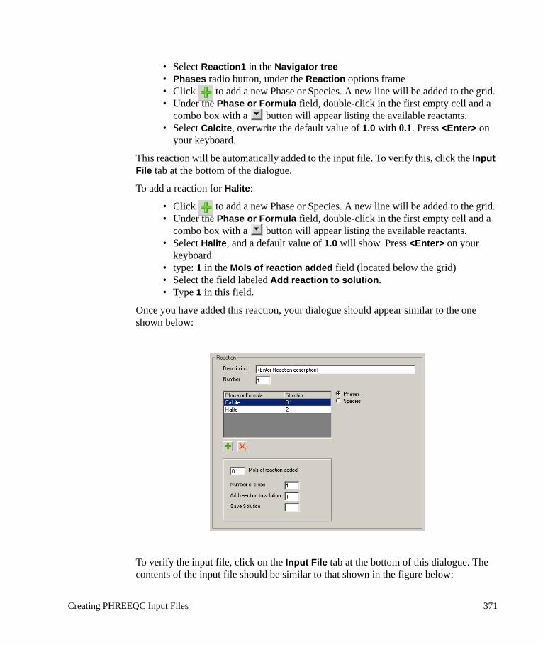
• Select Reaction1 in the Navigator tree• Phases radio button, under the Reaction options frame• Click to add a new Phase or Species. A new line will be added to the grid. • Under the Phase or Formula field, double-click in the first empty cell and a

combo box with a button will appear listing the available reactants. • Select Calcite, overwrite the default value of 1.0 with 0.1. Press <Enter> on

your keyboard.

This reaction will be automatically added to the input file. To verify this, click the Input File tab at the bottom of the dialogue.

To add a reaction for Halite:

• Click to add a new Phase or Species. A new line will be added to the grid. • Under the Phase or Formula field, double-click in the first empty cell and a

combo box with a button will appear listing the available reactants. • Select Halite, and a default value of 1.0 will show. Press <Enter> on your

keyboard.• type: 1 in the Mols of reaction added field (located below the grid)• Select the field labeled Add reaction to solution. • Type 1 in this field.

Once you have added this reaction, your dialogue should appear similar to the one shown below:

To verify the input file, click on the Input File tab at the bottom of this dialogue. The contents of the input file should be similar to that shown in the figure below:

Creating PHREEQC Input Files 371

You may now run PHREEQC with these reaction and solution options.

7.4 Running PHREEQC SimulationOnce you have specified the necessary Solutions and Reaction Steps, you are ready to run the simulation. Before doing so, it is recommended that you verify the contents of the input file. Once this is finished, click the [Run] button to run the simulation.

The PHREEQC simulation will run in the background as a DOS application inside a DOS window. Once the simulation is finished, you can verify the results by clicking the Output File tab (at the bottom of the main PHREEQC dialogue) and scan this for any error messages. The output from the PHREEQC run can be viewed by clicking on the Output File tab, or on the Spreadsheet tab.

372 Chapter 7: GeoChemical Modeling with PHREEQC

References

Appelo, C.A.J. and Postma, D., 2005, 2nd ed: Geochemistry Groundwater and Pollution. A.A. Balkeema. Rotterdam, 634 p.

Balderer, W., Pearson , F. J. jr., and Soreau, S., 1991: Sulphur and Oxygen Isotopes in Sulfate and Sulfide. In F. J. J. Pearson, W. Balderer, H. H. Loosli, B. E. Lehmann, A. Matter, T. Peters, H. Schmassmann, & A. Gautschi (Eds.), Applied Isotope Hydrogeology a case Study in northern Switzerland - NTB 88-01 Amsterdam - Oxford - New York - Tokyo: Elsevier.

Balderer, W., Pearson, F. J., Rauert, W., and Stichler, W., 1991: Isotopic Composition of Groundwater. In: F. J. Pearson, W. Balderer, H. H. Loosli, B. E. Lehmann, A. Matter, T. Peters, H. Schmassmann, & A. Gautschi (Eds.), Applied Isotope Hydrogeology - A Case Study In Northern Switzerland. - Studies in Environmental Science (pp. 98-115).

Drever, J. I., 1982: The Geochemistry of Natural Waters. Prentice Hall, New Jersey, Amsterdam: Elsevier, 437 p.

Fournier, R. O., 1981: Application of Water Chemistry to Geothermal Exploration and Reservoir Engineering. In: L. Rybach & L. J. P. Muffler (Eds.), Geothermal Systems: Principles and Case Histories, New York: Wiley, pp. 109-143.

Giggenbach, W.F., 1988. Geothermal solute equilibria. Derivation of Na-K-Mg-Ca geoindicators. Geochim Cosmochim. Acta, 52: pp. 2749-2765.

Giggenbach, W.F., 1989: The chemical and isotopic position of Ohaaki field within the Taupo Volcanic Zone. Proc. Eleventh N.Z. Geothermal Workshop, Aukland: pp. 81-88.

Hounslow, A.W. 1995: Water Quality Data – Analysis and Interpretation. CRC Press LLC. pp. 75-85.

Howard, P.H. et al. 1991: Handbook of Environmental Degradation Rates, Lewis Publishers, 775 p.

Kharaka, Y. K., Gunter, W. D., Affarwall, P. K., Perkins, E. H., and De Braal, J. D., 1988: Solmineq.88: A computer Program Code for Geochemical Modelling of Water-Rock Interactions. In U.S.Geological Survey Water Investigations Report 88-05.

Kharaka, Y. K., and Mariner, R. H., 1989: Chemical Geothermometers and their Application to formation waters from sedimentary basins. In: N. D. Näser & T. H.

373 References

Lin, S., 2001: Water and wastewater calculations manual. McGraw-Hill, New York. pp. 6-8.

Lloyd, J. W., and Heathcote, J. A., 1985: Natural inorganic hydrochemistry in relation to groundwater - An Introduction. Oxford: Clarendon Press.

McCulloh (Eds.), Thermal History of Sedimentary Basins; Methods and Case Histories, Springer Verlag, pp. 99-117.

Nordstrom, D. K., Plummer, L. N., Langmuir, D., Busenberg, E., Man, H. M., Jones, B. F., and Parkhurst, D. L., 1990: Revised Chemical Equilibrium Data for Major Water-Mineral Reactions and their Limitations. In: D. C. Melchior & R. L. Bassett (Eds.), Chemical Modelling of Aqueous Systems Washington: American Chemical Society.

Parkhurst D.K., Thorenston D.C. and Plummer N.L., 1980: PHREEQE - A computer program for geochemical calculations. U.S. Geological Survey Water Resource Investigations 80-96, 210 p. http://gwrp.cciw.ca/gwrp/software/software.html

Pearson, F. J. J., Lolcama, J. L., and Scholtis, A., 1989: Chemistry of Waters in the Böttstein, Weiach, Riniken, Schafisheim, Kaisten and Leuggern Boreholes: A Hydrochemically consistent Data Set. No. NTB 86-19, Nagra.

ReedM.and Spycher N., 1984: Calculations of pH and mineral equilibria in hydrothermal waters with application to geothermy and studies of boiling and dilution. Geochimica and Cosmochimica Acta, 48, pp. 1479-1492.

Stumm, W., and Morgan, J. J., 1981: Aquatic chemistry (2nd ed.). New York: John Wiley & Sons.

Tukey J.W., 1977: Exploratory Data Analysis, Addison-Wesley, Reading, Massachusetts, USA. pp. 39-43.

374 References

Appendices

Appendix A: Troubleshooting and Frequently Asked QuestionsThe following list provides answers to some of the most common problems encountered by users of AquaChem. Please review this list of frequently asked questions before contacting SWS Technical Support for assistance with your project.

Q 1: My sample symbols do not show up on the plot.A1. Check that you have assigned symbols to that sample(s).A2. Ensure the symbol group is active for the plots. This can be set in the Plots >

Define Symbol or Line dialogue.A3. Ensure that you have entered data for each parameter required by that plot.

Q 2: My symbols show up on the plot colored in red, even though I have assigned another color to this symbol.

A. The red colored symbols correspond to the samples which are selected in the active list. This indicates you are using the Identify Samples option in the Define Symbol or Line dialogue. Disable this option and the symbols will no longer be identified.

Q 3. After I import data, the data does not appear correctly or does not appear at all.A1. Check that you have a value for each sample for each parameter in your source

file.A2. Ensure that you have selected the correct Delimiter during the import routine.A3. Check your data source file to ensure that there are no extra spaces between

columns or rows of data.

Q 4: During data import, I get an error “Column must be assigned to CAS Registry #.”A1. Ensure that you have specified the correct import format. For this warning, you

should typically try the Samples as Rows in the Format field. A2. If your data source file does not contain CAS Registry #’s, ensure that this

option is disabled during the data import.

Q 5: During data import, I get error “Column must be assigned to SampleID or StationID.”A1. Ensure that you have specified the correct import format. For this warning,

you should typically try the Samples as Rows in the Format field.A2. Ensure that you have mapped at least one of your text fields as the StationID

and SampleID.

375

Q 6: Some of my samples or stations no longer appear in the active list.A. Since samples and stations are actively linked in the database, when you

temporarily omit a station, the corresponding samples will be removed from the active list. Likewise, when you remove all samples assigned to a given station, this station will be temporarily removed from the active list. To restore all samples or stations press the Show all button in the active samples list dialogue, or select Filter from the main menu and then Show all option.

Q 7: In the print options window, part of the plot is cut off by the print template.A. Be sure to select the print template first, then load the plot on top of the template.

This will ensure the page margins are set correctly, and will not cut off sections of the plot.

Q 8: After I enter a value for a measured parameter, the 0 after the decimal place is cut off (for example, 7.20 in entered, however AquaChem displays this as 7.2).

A. This can be corrected by modifying the parameter format. Go to File > Database > Parameters. Select the appropriate measured parameter, and modify the format. Disable the Auto option, and increase the number of decimal places to the desired value.

Q 7: Is it possible to create two unique Piper plots showing two different sample groups?

A. AquaChem will not allow for multiple Piper plot windows showing two distinct sample groups, at the same time. Since plots are created from information based on the active samples list, any changes that are made in the active list will immediately impact any open plot windows. The plots must be created individually.

376 Appendix A

Appendix B: Configuring an ODBC ConnectionTo use the AquaChem - HGA linking feature, you must configure an ODBC connection for your HGA SQL Server database. This can be done using Windows native ODBC Data Source Administrator tool. The following describes the steps to configure an ODBC connection:

Please note that the following may vary slightly between different operating systems. The following steps are described for Windows XP.

1. Go to Start / Settings / Control Panel /Administrative Tools2. Select Data Sources (ODBC). The following windows dialog will display:

From the User DSN tab, click the [Add] button.

3. From the Create New Data Source dialog, select SQL Server and then click the [Finish] button

377

4. From the Create a New Data Source to SQL Server dialog, enter the fol-lowing information, and then click [Next].

Name: Enter a name for the new data source

Description: Enter a description for the new data source (optional)

Server: Specify the server and instance that contains the HGA database. If the database resides on your local machine, then you would specify your computer name, instead of a server name.

5. In the next dialog, select the appropriate SQL Server authentication option. In most cases, you can leave the default settings and then click the [Next] button.

378 Appendix A

6. Choose your HGA database from the Change the default database to: combobox and select [Next].

379

7. In the next dialog, leave the default settings, and select the [Finish] button.

8. Finally, click the [Test Data Source...] button to test your ODBC connec-tion.

If successful, click [Ok] to finish. If the test failed, review the ODBC settings to ensure that they are correctly defined.

380 Appendix A

AActive List Window

Options 102Aliases 147AquaChem Database 129

Aliases 147Calculations 162Compress 130Create a new database 23, 50Look Up Tables 148Parameter Groups 141Parameters 131Ranges 158Thermometers 160Water Quality Standards 150

AquaChem Function 121AquaChem Tool Bar 20

CCalculate facies 122Calculations 162

AquaChem Calculations 165Calculators 121

AquaChem Function 296Calculate facies 307Decay Calculator 297Find Missing Major Ion 300Formula Weight Calculator 301Special Conversions 303Species Converter 305Unit Calculator 306Volume Concentration Converter 302

Censored data 91Correlation Matrix 120

DDecay Calculator 121, 297

EEdit

Copy 93Cut 93Find 94Paste 93Replace 93

ExportData 64Plot Image 63Text File 62To ESRI Shapefile 63To Visual MODFLOW 66

FFile

Close 53Database 129Export 62Import 54

New 49Open 52Preferences 86Print 72Save Database 53Save Database Template 53

Filter Menu 105Invert Selection 106Open Selection 106Save Selection 107Select Associate Samples or Stations 106

Find Missing Major Ion 121Formula Weight Calculator 122

GGenerate PHT3D Input 331Geothermometers 160

Creating 162

HHelp

Online Help 7

IImport

Sample Data 27, 54Installing AquaChem 5

LLink to HGA database 67LookUp Tables 148, 316

Degradation Rates 317Links 318Organic Compounds 319Periodic Table 317PHREEQC Phases 317Preservation Methods 319

NNormality, Tests for 120

OODBC 377Open Database from V. 3.7 10Outlier Tests 120

PParameters

Adding and Creating 137Deleting Parameters 139Details 133Groups 141Mandatory Parameters 140

PHREEQCCreate Input File 327How to Create Input Files 343

381

Model pH 323Model Samples 321PHREEQC for Windows 329PHREEQC-Interactive 328Preferences 344

PHREEQC, connect to files 90Plots 175

Automatic Plot Title Preferences 89Box and Whisker 197Configurations 116, 189Copy to Clipboard 192Create 116Customize global options 88Depth Profile 201Dialogues

Format 186Labels 187Legend 182Line 183Symbols 180Title 177

Durov Plot 203Geothermometer Plot 205Giggenbach Triangle 207Histogram 208Identify Plot Data 118, 191Ludwig-Langelier 209Map Plot 211Options 105, 176Pie 221Piper Diagram 223Printing 193Radial Diagram 227Save as Metafile 192Scatter Plot 229Schoeller Plot 230Show Sample Data 117Stiff Diagram 231Ternary Plot 233Time Series Plot 236Wilcox Diagram 240

PreferencesActive Graphs 89PHREEQC 90Plot Titles 89Symbol Fonts 89

PrintPlots 193Reports 246

RRanges 158

Creating New 159Report Designer 278

Designing a New Report 280Reports 118

Compare Sample 119Compare Samples 246Mix Samples 119, 249Options 105, 243

Print 47Rock Source Deduction 119, 253Sample Summary 276Save 46Statistics 255

Correlation Matrix 120, 263Outlier Tests 120, 271Summary Statistics 119, 255Tests for normality 120, 274Trend Analysis 120, 265

User Defined 120Water Quality Standards 119, 252

SSample

Assign Station 115Assign Symbols 109Clone 109Create New 107Delete 109Edit 109Representative 115

Sample Details Window 14Options 103

Sample ListOptions 102

Save as Template 54Special Conversions 122Species Converter 122Station

Create new 107Delete 109Edit 109

Station Details Window 17Summary Statistics 119Symbols

Assign 109Automatically Generate 113Create 112Create new symbol group 111Edit 112Symbol Fonts 89

TTable View 97

Create 98Default 102Options 104

Template DesignerCreating new templates 81

Tools 121Calculators 121

AquaChem Function 121, 296Calculate facies 122, 307Decay Calculator 121, 297Find Missing Major Ion 121, 300Formula Weight Calculator 122, 301Special Conversions 122, 303

382

Species Converter 122, 305Unit Calculator 122, 306Volume Concentration Converter 122, 302

Look Up Tables 124Degradation Rates 124, 317Links 124, 318Organic Compounds 124, 319Periodic Table 124, 317PHREEQC Phases 124, 317Preservation Methods 125, 319

Modeling 125, 319Calculate Eh 125, 324Calculate pH 125, 323Calculate SIs and Activities 125, 321PHREEQC (Advanced) 126, 328PHREEQC (Basic) 126, 327

QA/QC 122, 311Compare Duplicates 123, 313Find Duplicates 123, 315Highlight Duplicates 124, 316Highlight Nondetects 123, 315Highlight Outliers 124, 316Reliability Check 122, 311

Trend Analysis 120

UUnit Calculator 122

VVolume Concentration Converter 122

WWater Quality Standards 150

Create 153Customize highlight colors 87Preferences and Settings 87

383

384