Embed Size (px)
Citation preview

Approximation algorithms for Euler genusand related problems
Chandra Chekuri Anastasios Sidiropoulos
February 3, 2014
Slides based on a presentation of Tasos Sidiropoulos

Graphs and topology
Theorem (Kuratowski, 1930)
A graph is planar if and only if it does not contain K5 and K3,3 asa topological minor.
Theorem (Wagner, 1937)
A graph is planar if and only if it does not contain K5 and K3,3 asa minor.

Graphs and topology
Theorem (Kuratowski, 1930)
A graph is planar if and only if it does not contain K5 and K3,3 asa topological minor.
Theorem (Wagner, 1937)
A graph is planar if and only if it does not contain K5 and K3,3 asa minor.

Graphs and topology
Theorem (Kuratowski, 1930)
A graph is planar if and only if it does not contain K5 and K3,3 asa topological minor.
Theorem (Wagner, 1937)
A graph is planar if and only if it does not contain K5 and K3,3 asa minor.

Minors and Topological minors
DefinitionA graph H is a minor of G if H is obtained from G by a sequenceof edge/vertex deletions and edge contractions.
DefinitionA graph H is a topological minor of G if a subdivision of H isisomorphic to a subgraph of G .

Planarity
planar graph non-planar graph

Planarity
planar graphnon-planar graph

What about other surfaces?
sphere torus double torus triple torus
g = 0 g = 1 g = 2 g = 3
real projective plane Klein bottle
k = 1 k = 2

What about other surfaces?
sphere torus double torus triple torusg = 0 g = 1 g = 2 g = 3
real projective plane Klein bottlek = 1 k = 2

Genus of graphs
DefinitionThe orientable (reps. non-orientable) genus of a graph G is theminimum k, such that G admits an embedding into a surface oforientable (resp. non-orientable) genus k .
I Graph genus of a graph quantifies “closeness” to planarity.
genus(K5) = 1 genus(teapot) ≤ 1 genus(bridge) ≤ 24

Euler genus
For any surface S,
eg(S) := min2 · genus(S), nonorientable-genus(S)
Euler characteristic: For any triangulation of S, with v vertices, eedges, and f faces, we have
χ(S) := v − e + f = 2− eg(S)
For any graph G ,
eg(G ) := ming ∈ N≥0 : G embeds into a surface S, with eg(S) = g

Euler genus
For any surface S,
eg(S) := min2 · genus(S), nonorientable-genus(S)
Euler characteristic: For any triangulation of S, with v vertices, eedges, and f faces, we have
χ(S) := v − e + f = 2− eg(S)
For any graph G ,
eg(G ) := ming ∈ N≥0 : G embeds into a surface S, with eg(S) = g

Euler genus
For any surface S,
eg(S) := min2 · genus(S), nonorientable-genus(S)
Euler characteristic: For any triangulation of S, with v vertices, eedges, and f faces, we have
χ(S) := v − e + f = 2− eg(S)
For any graph G ,
eg(G ) := ming ∈ N≥0 : G embeds into a surface S, with eg(S) = g

Graph minors
DefinitionA family of graphs G is minor-closed if for any G ∈ G all minors ofG are also in G.
DefinitionA property P of graphs is minor-closed if all graphs satisfying Pform a minor-closed family.

Minor-closed properties
I Planarity
I Orientable genus g , for some g > 0.
I Nonorientable genus g , for some g > 0.
I Euler genus g , for some g > 0.
I k-apex, for some k > 0.
I Linkless embeddability in R3.
I Treewidth k , for some k > 0.

Minor-closed properties
I Planarity
I Orientable genus g , for some g > 0.
I Nonorientable genus g , for some g > 0.
I Euler genus g , for some g > 0.
I k-apex, for some k > 0.
I Linkless embeddability in R3.
I Treewidth k , for some k > 0.

Minor-closed properties
I Planarity
I Orientable genus g , for some g > 0.
I Nonorientable genus g , for some g > 0.
I Euler genus g , for some g > 0.
I k-apex, for some k > 0.
I Linkless embeddability in R3.
I Treewidth k , for some k > 0.

Minor-closed properties
I Planarity
I Orientable genus g , for some g > 0.
I Nonorientable genus g , for some g > 0.
I Euler genus g , for some g > 0.
I k-apex, for some k > 0.
I Linkless embeddability in R3.
I Treewidth k , for some k > 0.

Minor-closed properties
I Planarity
I Orientable genus g , for some g > 0.
I Nonorientable genus g , for some g > 0.
I Euler genus g , for some g > 0.
I k-apex, for some k > 0.
I Linkless embeddability in R3.
I Treewidth k , for some k > 0.

Minor-closed properties
I Planarity
I Orientable genus g , for some g > 0.
I Nonorientable genus g , for some g > 0.
I Euler genus g , for some g > 0.
I k-apex, for some k > 0.
I Linkless embeddability in R3.
I Treewidth k , for some k > 0.

Minor-closed properties
I Planarity
I Orientable genus g , for some g > 0.
I Nonorientable genus g , for some g > 0.
I Euler genus g , for some g > 0.
I k-apex, for some k > 0.
I Linkless embeddability in R3.
I Treewidth k , for some k > 0.

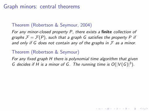
Graph minors: central theorems
Theorem (Robertson & Seymour, 2004)
For any minor-closed property P, there exists a finite collection ofgraphs F = F(P), such that a graph G satisfies the property P ifand only if G does not contain any of the graphs in F as a minor.
Theorem (Robertson & Seymour)
For any fixed graph H there is polynomial time algorithm that givenG decides if H is a minor of G. The running time is O(|V (G )|3).
I Implies existence of an efficient algorithm for testing anyminor-closed property.
Running time improved to O(|V (G )|2) by[Kawarabayashi-Kobayashi-Reed ’12].

Computing the Euler genus of a graph
Given n-vertex graph G , decide whether eg(G ) ≤ g , for someg ≥ 0.
I O(n3 · f (g))-time [Robertson & Seymour]
I O(n · f ′(g))-time [Mohar ’99]
I O(n · 2O(g))-time [Kawarabayashi, Mohar & Reed ’08]
I NP-hard [Thomassen ’89]
The exponential dependence on g is necessary!

Graphs and topology
To KASIMIR KURAT0WSK1 Who gave Ks and Ki3
To those who thmujht planarity Was nothing hut topology.
KM:

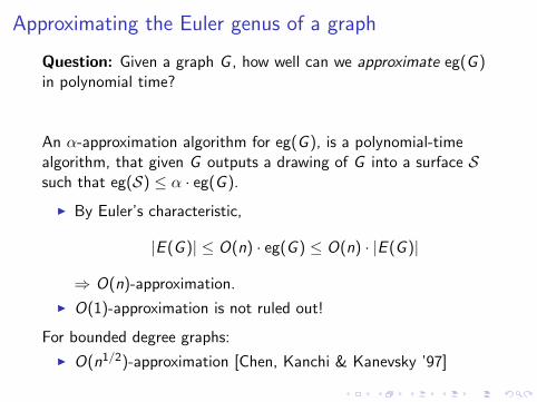
Approximating the Euler genus of a graph
Question: Given a graph G , how well can we approximate eg(G )in polynomial time?
An α-approximation algorithm for eg(G ), is a polynomial-timealgorithm, that given G outputs a drawing of G into a surface Ssuch that eg(S) ≤ α · eg(G ).
I By Euler’s characteristic,
|E (G )| ≤ O(n) · eg(G ) ≤ O(n) · |E (G )|
⇒ O(n)-approximation.
I O(1)-approximation is not ruled out!
For bounded degree graphs:
I O(n1/2)-approximation [Chen, Kanchi & Kanevsky ’97]

A Pseudo-Approximation
Theorem (Makarychev, Nayyeri & Sidiropoulos ’12)
There is a polynomial-time algorithm, that given a Hamiltonialgraph G (along with a Hamilton path P) and integer g, eitheroutputs a drawing of G into a surface S such thateg(S) ≤ O(gO(1)) or correctly decides that eg(G ) > g.

Main Result
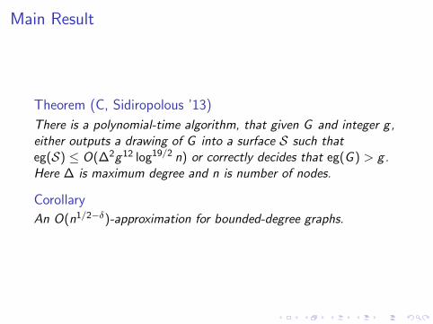
Theorem (C, Sidiropolous ’13)
There is a polynomial-time algorithm, that given G and integer g,either outputs a drawing of G into a surface S such thateg(S) ≤ O(∆2g12 log19/2 n) or correctly decides that eg(G ) > g.Here ∆ is maximum degree and n is number of nodes.
Corollary
An O(n1/2−δ)-approximation for bounded-degree graphs.
Main Result
Theorem (C, Sidiropolous ’13)
There is a polynomial-time algorithm, that given G and integer g,either outputs a drawing of G into a surface S such thateg(S) ≤ O(∆2g12 log19/2 n) or correctly decides that eg(G ) > g.Here ∆ is maximum degree and n is number of nodes.
Corollary
An O(n1/2−δ)-approximation for bounded-degree graphs.

Beyond Euler genus
Further applications for bounded degree graphs.
I gO(1)-approximation for orientable genus.
I kO(1)-approximation for crossing number.
I kO(1)-approximation minimum edge/vertex planarization.
Beyond Euler genus
Further applications for bounded degree graphs.
I gO(1)-approximation for orientable genus.
I kO(1)-approximation for crossing number.
I kO(1)-approximation minimum edge/vertex planarization.

Beyond Euler genus
Further applications for bounded degree graphs.
I gO(1)-approximation for orientable genus.
I kO(1)-approximation for crossing number.
I kO(1)-approximation minimum edge/vertex planarization.
Some details of the algorithm

Tree decompositions and TreewidthTree Decomposition
a b
c
d e
f
g h
a b c a c f
d e c
a g f g h
Example from Bodlaender’s talk
G=(V,E) T=(VT, ET)
t Xt = d,e,c ! V
A tree decomposition of G is a tree(T = (VT ,ET ) and collectionof sets/bags Xt ⊆ V (G ) : t ∈ VT such that
I ∪t∈VTXt = V (G ).
I For every u, v ∈ E (G ), there is t ∈ VT s. t. u, v ⊆ Xt .
I For every v ∈ V (G ), the set t ∈ VT : v ∈ Xt forms aconnected subtree of T .
The width of the decomposition is defined to be maxt∈VT|Xt | − 1.

Tree decompositions and Treewidth
DefinitionThe treewidth of a graph G , denoted by tw(G ), is the minimumwidth of a tree decomposition for G .
Examples:
I For any tree T , tw(T ) = 1.
I For any cycle C , tw(C ) = 2.
I For a complete graph Kn, tw(Kn) = n − 1.
I For any (r × r)-grid G , tw(G ) = Θ(r). Thus planar graphscan have “large” treewidth.

Treewidth / grid-minor duality
Theorem (Robertson & Seymour ’86)
There is a function f such that any graph G with tw(G ) ≥ f (k)contains a clique of size k or the k × k grid as a minor.
Theorem: tw(G) ! f(k) implies G contains a clique minor of size k or a grid minor of size k
Robertson-Seymour Grid-Minor Theorem(s)
Corollary (Grid-minor theorem)
tw(G ) ≥ f (k) implies G contains a√
k ×√
k grid as a minor.
The grid is a canonical obstruction for small treewidth.

Treewidth / grid-minor duality: quantitative bounds
Theorem (Robertson, Semour, Thomas ’94)
Let G be a graph such that tw(G ) ≥ 2O(k5) then G contains a gridminor of size k.If G is a planar graph then G contains a grid-minor of sizetw(G )/6.
Theorem (Demaine et al. ’05)
Let G be a graph of Euler genus g, then G contains a “flat” gridminor of size Ω(tw(G )/(g + 1)).
Theorem (C, Chuzhoy ’13)
Let G be a graph such that tw(G ) ≥ k100 then G contains a gridminor of size k.

Treewidth paradigm in algorithms
I If G has “small” (constant) treewidth, solve problemefficiently or approximately. Running time typically dependsexponentially on tw(G ).
I If G has “large” treewidth use obstruction given by structuressuch as grids

High-level overview
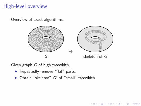
Overview of exact algorithms.
→G
skeleton of G
Given graph G of high treewidth.
I Repeatedly remove “flat” parts.
I Obtain “skeleton” G ′ of “small” treewidth.
I Compute a drawing for the skeleton G ′ exactly.
I Extend the drawing to G .
High-level overview
Overview of exact algorithms.
→G skeleton of G
Given graph G of high treewidth.
I Repeatedly remove “flat” parts.
I Obtain “skeleton” G ′ of “small” treewidth.
I Compute a drawing for the skeleton G ′ exactly.
I Extend the drawing to G .

High-level overview
Overview of exact algorithms.
→G skeleton of G
Given graph G of high treewidth.
I Repeatedly remove “flat” parts.
I Obtain “skeleton” G ′ of “small” treewidth.
I Compute a drawing for the skeleton G ′ exactly.
I Extend the drawing to G .

High-level overview
Overview of exact algorithms.
→G skeleton of G
Given graph G of high treewidth.
I Repeatedly remove “flat” parts.
I Obtain “skeleton” G ′ of “small” treewidth.
I Compute a drawing for the skeleton G ′ exactly.
I Extend the drawing to G .

Flatness and embeddings
DefinitionLet G be a graph, and let H be a planar subgraph of G . We saythat H is flat if there exists a planar drawing of H, such that alledges u, v ∈ E (G ), with u ∈ V (H), v ∈ V (G ) \ V (H), thevertex u is on the outer face of H.
Theorem (Mohar ’92)
Let G be a graph of Euler genus g, and let H be a flat (r × r)-gridminor H in G , for some r > 10 · g. Then, in any drawing of G intoa surface of genus g, the “central part” of H is embedded inside adisk.

High-level overview
Overview of exact algorithms.
→G skeleton of G
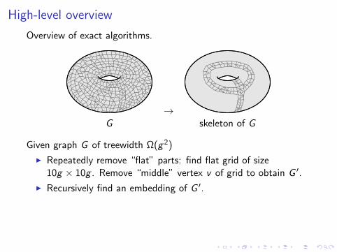
Given graph G of treewidth Ω(g2)
I Repeatedly remove “flat” parts: find flat grid of size10g × 10g . Remove “middle” vertex v of grid to obtain G ′.
I Recursively find an embedding of G ′.
I Extend the drawing to G by placing v in the middle of grid.
I Recursion stops when tw(G ) is “small”, tw(G ) = O(g2).Compute a drawing exactly in time f (g)poly(n).
High-level overview
Overview of exact algorithms.
→G skeleton of G
Given graph G of treewidth Ω(g2)
I Repeatedly remove “flat” parts: find flat grid of size10g × 10g . Remove “middle” vertex v of grid to obtain G ′.
I Recursively find an embedding of G ′.
I Extend the drawing to G by placing v in the middle of grid.
I Recursion stops when tw(G ) is “small”, tw(G ) = O(g2).Compute a drawing exactly in time f (g)poly(n).

High-level overview or our algorithm
G approximate skeleton rigid skeleton
Given graph G of high treewidth.
I Repeatedly remove “flat” parts.
I Obtain “skeleton” G ′ of small treewidth.
I Compute a “rigid skeleton” G ′′.
I Compute a drawing for G ′′ approximately.
I Modify the drawing to obtain a drawing for G .

Planarizing graphs of small treewidth, and small genus
LemmaThere exists a polynomial time algorithm which given a graph G oftreewidth t, and an integer g ≥ 0, either correctly decides thateg(G ) > g, or it outputs a set X ⊆ V (G ), such that
I |X | = O(gt log3/2 n).
I G \ X is planar.

Planarizing graphs of small treewidth, and small genus
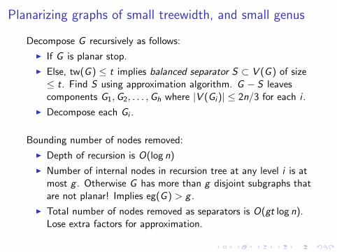
Decompose G recursively as follows:
I If G is planar stop.
I Else, tw(G ) ≤ t implies balanced separator S ⊂ V (G ) of size≤ t. Find S using approximation algorithm. G − S leavescomponents G1,G2, . . . ,Gh where |V (Gi )| ≤ 2n/3 for each i .
I Decompose each Gi .
Bounding number of nodes removed:
I Depth of recursion is O(log n)
I Number of internal nodes in recursion tree at any level i is atmost g . Otherwise G has more than g disjoint subgraphs thatare not planar! Implies eg(G ) > g .
I Total number of nodes removed as separators is O(gt log n).Lose extra factors for approximation.
Planarizing graphs of small treewidth, and small genus
Decompose G recursively as follows:
I If G is planar stop.
I Else, tw(G ) ≤ t implies balanced separator S ⊂ V (G ) of size≤ t. Find S using approximation algorithm. G − S leavescomponents G1,G2, . . . ,Gh where |V (Gi )| ≤ 2n/3 for each i .
I Decompose each Gi .
Bounding number of nodes removed:
I Depth of recursion is O(log n)
I Number of internal nodes in recursion tree at any level i is atmost g . Otherwise G has more than g disjoint subgraphs thatare not planar! Implies eg(G ) > g .
I Total number of nodes removed as separators is O(gt log n).Lose extra factors for approximation.
Handling “small” treewidth case
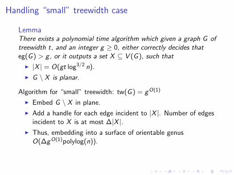
LemmaThere exists a polynomial time algorithm which given a graph G oftreewidth t, and an integer g ≥ 0, either correctly decides thateg(G ) > g, or it outputs a set X ⊆ V (G ), such that
I |X | = O(gt log3/2 n).
I G \ X is planar.
Algorithm for “small” treewidth: tw(G ) = gO(1)
I Embed G \ X in plane.
I Add a handle for each edge incident to |X |. Number of edgesincident to X is at most ∆|X |.
I Thus, embedding into a surface of orientable genusO(∆gO(1)polylog(n)).
Caveat: we cannot use this directly

Handling “small” treewidth case
LemmaThere exists a polynomial time algorithm which given a graph G oftreewidth t, and an integer g ≥ 0, either correctly decides thateg(G ) > g, or it outputs a set X ⊆ V (G ), such that
I |X | = O(gt log3/2 n).
I G \ X is planar.
Algorithm for “small” treewidth: tw(G ) = gO(1)
I Embed G \ X in plane.
I Add a handle for each edge incident to |X |. Number of edgesincident to X is at most ∆|X |.
I Thus, embedding into a surface of orientable genusO(∆gO(1)polylog(n)).
Caveat: we cannot use this directly

Handling “large” treewidth
tw(G ) = t > g10: want to find “flat” grid minor in poly(g , n) time.
Idea:
I G has a grid minor H of size Ω(t/g)× Ω(t/g).
I From lemma can remove O(gt) nodes X such thatG ′ = G − X is planar.
I G ′ will have large treewidth if we can show that H − X has alarge grid minor.
I Recover grid minor from G ′.

Persistence of grid minors
Lemma (Eppstein ’13)
Let r , f ≥ 1. Let G be the (r × r)-grid, and X ⊂ V (G ), with|X | = f . Then, G \ X contains the (r ′ × r ′)-grid as a minor, wherer ′ = Θ(minr , r2/f ).
f = O(r) f = Ω(r)

Persistence of grid minors
Lemma (Eppstein ’13)
Let r , f ≥ 1. Let G be the (r × r)-grid, and X ⊂ V (G ), with|X | = f . Then, G \ X contains the (r ′ × r ′)-grid as a minor, wherer ′ = Θ(minr , r2/f ).
f = O(r) f = Ω(r)

Grid minors and planarization
Corollary (Chekuri, S ’13)
Let G be a graph of Euler genus g ≥ 1, and treewidth t ≥ 1. Thereis a polynomial time algorithm to compute a set X ⊆ V (G ), with|X | = (gt log5/2 n), and a planar connected component of G \ X
containing the (r ′ × r ′)-grid as a minor, with r ′ = Ω(
tg3 log5/2 n
).
Thus if t > g10 can find a flat grid minor of size Ω(g7). This gridhas to be rigidly embedded inside a disk in any embedding of Ginto a surface of genus ≤ g .

Flat grid minors to Skeleton
G approximate skeleton rigid skeleton
Given graph G of high treewidth.
I Repeatedly remove “flat” grid minors.
I Obtain “skeleton” G ′ of small treewidth.
To extend drawing of skeleton need to define it carefully.Need to “merge” the multiple flat grid minors properly.

Skeleton
I Removed parts form “patches”(C1,X1), (C2,X2), . . . , (Ck ,Xk).
I Each patch (Ci ,Xi ) consists of a set of nodes Xi ⊂ V and acycle Ci ⊂ Xi
I The patches are disjoint
I In any drawing of G into a surface of Euler genus g , eachpatch (Ci ,Xi ) has to be drawn in a disk with Ci as itsboundary.
I Skeleton that remains has “small” treewidth: O(gO(1)).

Making Skeleton rigid
I Embed skeleton G ′ using the small treewidth algorithm
I Insert patches into the embedding of the skeleton
I Problem: The cycles Ci for the pathches may not be enclose adisk in the embedding of G ′ since embedding is not into agenus g surface.
I Our fix: Framing

Making Skeleton rigid
I Embed skeleton G ′ using the small treewidth algorithm
I Insert patches into the embedding of the skeleton
I Problem: The cycles Ci for the pathches may not be enclose adisk in the embedding of G ′ since embedding is not into agenus g surface.
I Our fix: Framing

Making Skeleton rigid
I Embed skeleton G ′ using the small treewidth algorithm
I Insert patches into the embedding of the skeleton
I Problem: The cycles Ci for the pathches may not be enclose adisk in the embedding of G ′ since embedding is not into agenus g surface.
I Our fix: Framing
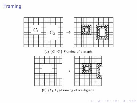
Framing
(a) C1,C2-Framing of a graph.
(b) C1,C2-Framing of a subgraph.

Planarizing Skeleton
Skeleton has treewidth O(gO(1)).
LemmaLet G ′ be skeleton of G with patches (X1,C1), . . . , (Xr ,Cr ). Thealgorithm either correctly decides that eg(G ) > g, or outputs a setX ⊆ V (G ) s.t.
I |X | = O(∆g12 log19/2 n).
I For every connected component H of G ′ \ X , the framing ofH is planar.

Extending embedding of Skeleton via Frames and Patches

Beyond Euler genus
Further applications for bounded degree graphs.
I gO(1)-approximation for orientable genus.
I kO(1)-approximation for crossing number.
I kO(1)-approximation minimum edge/vertex planarization.
Via a common framework that exploits the embedding given by thealgorithm to approximate the Euler genus

Representativity of face width of an embedding
DefinitionLet φ be an embedding of G into a surface S. A noose is a loop inS that only intersects φ(G ) at φ(V (G )). The length of a noose isthe number of vertices it intersects.
DefinitionThe representativity of φ is defined to be the smallest length of allnoncontractible nooses in φ.

Approximating Orientable genus
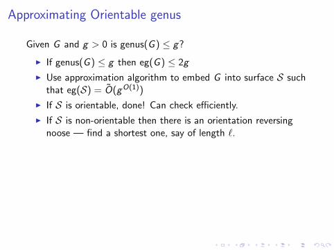
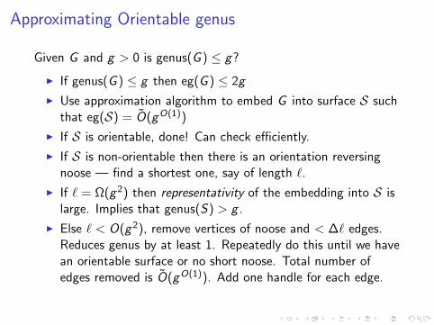
Given G and g > 0 is genus(G ) ≤ g?
I If genus(G ) ≤ g then eg(G ) ≤ 2g
I Use approximation algorithm to embed G into surface S suchthat eg(S) = O(gO(1))
I If S is orientable, done! Can check efficiently.
I If S is non-orientable then there is an orientation reversingnoose — find a shortest one, say of length `.
I If ` = Ω(g2) then representativity of the embedding into S islarge. Implies that genus(S) > g .
I Else ` < O(g2), remove vertices of noose and < ∆` edges.Reduces genus by at least 1. Repeatedly do this until we havean orientable surface or no short noose. Total number ofedges removed is O(gO(1)). Add one handle for each edge.

Approximating Orientable genus
Given G and g > 0 is genus(G ) ≤ g?
I If genus(G ) ≤ g then eg(G ) ≤ 2g
I Use approximation algorithm to embed G into surface S suchthat eg(S) = O(gO(1))
I If S is orientable, done! Can check efficiently.
I If S is non-orientable then there is an orientation reversingnoose — find a shortest one, say of length `.
I If ` = Ω(g2) then representativity of the embedding into S islarge. Implies that genus(S) > g .
I Else ` < O(g2), remove vertices of noose and < ∆` edges.Reduces genus by at least 1. Repeatedly do this until we havean orientable surface or no short noose. Total number ofedges removed is O(gO(1)). Add one handle for each edge.

Some open problems
I Is there a O(1)-approximation for Euler genus?
I Can we remove the bounded-degree assumption in ouralgorithm?
I Improve the dependence on g?
I Which other minor-closed properties admit similarapproximation algorithms? Can we approximate the largestclique-minor size?

Some open problems
I Is there a O(1)-approximation for Euler genus?
I Can we remove the bounded-degree assumption in ouralgorithm?
I Improve the dependence on g?
I Which other minor-closed properties admit similarapproximation algorithms? Can we approximate the largestclique-minor size?

Thank you!


![1. Introduction The Kuratowski Closure-Complement …nzjm.math.auckland.ac.nz/images/6/63/The_Kuratowski_Closure-Com… · The Kuratowski Closure-Complement Theorem 1.1. [29] If (X;T)](https://img.dokumen.tips/doc/110x75/5afec8997f8b9a256b8d8ca8/1-introduction-the-kuratowski-closure-complement-nzjmmath-the-kuratowski.jpg)