Embed Size (px)
Citation preview

arX
iv:1
907.
0482
6v1
[cs
.DS]
10
Jul 2
019
APPROXIMATELY COUNTING AND SAMPLING SMALL WITNESSES
USING A COLOURFUL DECISION ORACLE
HOLGER DELL∗, JOHN LAPINSKAS†, AND KITTY MEEKS‡
ABSTRACT. In this paper, we prove “black box” results for turning algorithms which decide whether or not
a witness exists into algorithms to approximately count the number of witnesses, or to sample from the set
of witnesses approximately uniformly, with essentially the same running time. We do so by extending the
framework of Dell and Lapinskas (STOC 2018), which covers decision problems that can be expressed as
edge detection in bipartite graphs given limited oracle access; our framework covers problems which can be
expressed as edge detection in arbitrary k-hypergraphs given limited oracle access. (Simulating this oracle
generally corresponds to invoking a decision algorithm.) This includes many key problems in both the fine-
grained setting (such as k-SUM, k-OV and weighted k-Clique) and the parameterised setting (such as induced
subgraphs of size k or weight-k solutions to CSPs). From an algorithmic standpoint, our results will make
the development of new approximate counting algorithms substantially easier; indeed, it already yields a new
state-of-the-art algorithm for approximately counting graph motifs, improving on Jerrum and Meeks (JCSS
2015) unless the input graph is very dense and the desired motif very small. Our k-hypergraph reduction
framework generalises and strengthens results in the graph oracle literature due to Beame et al. (ITCS 2018)
and Bhattacharya et al. (CoRR abs/1808.00691).
* IT UNIVERSITY OF COPENHAGEN, COPENHAGEN, DENMARK
† UNIVERSITY OF OXFORD, OXFORD, UK
‡ UNIVERSITY OF GLASGOW, GLASGOW, UK
E-mail addresses: [email protected], [email protected], [email protected].
Date: July 11, 2019.
The research leading to these results has received funding from the European Research Council under the European Union’s
Seventh Framework Programme (FP7/2007-2013) ERC grant agreement no. 334828. The paper reflects only the authors’ views
and not the views of the ERC or the European Commission. The European Union is not liable for any use that may be made of the
information contained therein. The research was also supported by a Royal Society of Edinburgh Personal Research Fellowship,
funded by the Scottish Government.
1
2 APPROXIMATELY COUNTING AND SAMPLING SMALL WITNESSES USING A COLOURFUL DECISION ORACLE
1. INTRODUCTION
Many decision problems reduce to the question: Does a witness exist? Such problems admit a natural
counting version: How many witnesses exist? For example, one may ask whether a bipartite graph contains
a perfect matching, or how many perfect matchings it contains. As one might expect, the counting version
is never easier than the decision version, and is often substantially harder; for example, deciding whether
a bipartite graph contains a perfect matching is easy, and counting the number of such matchings is #P-
complete [42]. However, even when the counting version of a problem is hard, it is often easy to approximate
well. For example, Jerrum, Sinclair and Vigoda [32] gave a polynomial-time approximation algorithm
for the number of perfect matchings in a bipartite graph. The study of approximate counting has seen
amazing progress over the last two decades, particularly in the realm of trichotomy results for general
problem frameworks such as constraint satisfaction problems, and is now a major field of study in its own
right [17, 18, 24, 27, 28]. In this paper, we explore the question of when approximating the counting version
of a problem is not merely fast, but essentially as fast as solving the decision version.
We first recall the standard notion of approximation in the field: For all real x, y > 0 and 0 < ε < 1, we
say that x is an ε-approximation to y if |x − y| < εy. Note in particular that any ε-approximation to zero
is itself zero, so computing an ε-approximation to N is always at least as hard as deciding whether N > 0holds. For example, it is at least as hard to approximately count the number of satisfying assignments of a
CNF formula (i.e. to ε-approximate #SAT) as it is to decide whether it is satisfiable at all (i.e. to solve SAT).
Perhaps surprisingly, in many cases, the converse is also true. For example, Valiant and Vazirani [43]
proved that any polynomial-time algorithm to decide SAT can be bootstrapped into a polynomial-time ε-approximation algorithm for #SAT, or, more formally, that a size-n instance of any problem in #P can
be ε-approximated in time poly(n, ε−1) using an NP-oracle. A similar result holds in the parameterised
setting, where Muller [40] proved that a size-n instance of any problem in #W[i] with parameter k can be
ε-approximated in time g(k) · poly(n, ε−1) using a W[i]-oracle for some computable function g : N → N.
Another such result holds in the subexponential setting, where Dell and Lapinskas [14] proved that the
(randomised) Exponential Time Hypothesis is equivalent to the statement: There is no ε-approximation
algorithm for #3-SAT which runs on an n-variable instance in time ε−22o(n).We now consider the fine-grained setting, which is the focus of this paper. Here, we are concerned with
the exact running time of an algorithm, rather than broad categories such as polynomial time, FPT time or
subexponential time. The above reductions all introduce significant overhead, so they are not fine-grained.
Here only one general result is known, again due to Dell and Lapinskas [14]. Informally, if the decision
problem reduces “naturally” to deciding whether an n-vertex bipartite graph contains an edge, then any
algorithm for the decision version can be bootstrapped into an ε-approximation algorithm for the counting
version with only O(ε−2polylog(n)) overhead. (See Section 1.1 for more details.)
The reduction of [14] is general enough to cover core problems in fine-grained complexity such as OR-
THOGONAL VECTORS, 3SUM and NEGATIVE-WEIGHT TRIANGLE, but it is not universal. In this paper,
we substantially generalise it to cover any problem which can be “naturally” formulated as deciding whether
a k-partite k-hypergraph contains an edge; thus we essentially recover the original result on taking k = 2.
For any problem which satisfies this property, our result implies that any new decision algorithm will auto-
matically lead to a new approximate counting algorithm whose running time is at most a factor of logO(k) nlarger. Our framework covers several reduction targets in fine-grained complexity not covered by [14], in-
cluding k-ORTHOGONAL VECTORS, k-SUM and EXACT-WEIGHT k-CLIQUE, as well as some key prob-
lems in parameterised complexity including weight-k CSPs and size-k induced subgraph problems. (Note
that the overhead of logO(k) n can be re-expressed as k2kno(1) using a standard trick, so an FPT decision
algorithm is transformed into an FPT approximate counting algorithm; see Section 1.3.)
In fact, we get more than fast approximate counting algorithms — we also prove that any problem in
this framework has an algorithm for approximately-uniform sampling, again with logO(k) n overhead over
decision. There is a well-known reduction between the two for self-reducible problems due to Jerrum,
Valiant and Vazirani [33], but it does not apply in our setting since it adds polynomial overhead.

APPROXIMATELY COUNTING AND SAMPLING SMALL WITNESSES USING A COLOURFUL DECISION ORACLE 3
In the parameterised setting, our results have interesting implications. Here, the requirement that the
hypergraph be k-partite typically corresponds to considering the “colourful” or “multicolour” version of
the decision problem, so our result implies that uncoloured approximate counting is essentially equivalent
to multicolour decision. We believe that our results motivate considerable further study of the relationship
between multicolour parameterised decision problems and their uncoloured counterparts.
Finally, we note that the applications of our results are not just complexity-theoretic in nature, but also
algorithmic. They give a “black box” argument that any decision algorithm in our framework, including
fast ones, can be converted into an approximate counting or sampling algorithm with minimal overhead.
Concretely, we obtain new algorithms for approximately counting and/or sampling zero-weight subgraphs,
graph motifs, and satisfying assignments for first-order models, and our framework is sufficiently general
that we believe new applications will be forthcoming.
In Section 1.1, we set out our main results in detail as Theorems 1 and 2, and discuss our edge-counting
reduction framework (which is of independent interest). We describe the applications of Theorems 1 and 2
to fine-grained complexity in Section 1.2, and their applications to parameterised complexity in Section 1.3.
1.1. The k-hypergraph framework. Given a k-hypergraph G = (V,E), write e(G) = |E|, and let
C(G) := (X1, . . . ,Xk) : X1, . . . ,Xk are disjoint subsets of V .We define the coloured independence oracle of G to be the function cINDG : C(G) → 0, 1 such that
cINDG(X1, . . . ,Xk) = 1 if G[X1, . . . ,Xk] has no edges, and cINDG(X1, . . . ,Xk) = 0 otherwise. Infor-
mally, we think of elements of C(G) as representing k-colourings of induced subgraphs of G, with Xi being
the i’th colour class; thus given a vertex colouring of an induced subgraph of G, the coloured independence
oracle outputs 1 if and only if no colourful edge is present. We consider a computation model where the
algorithm is given access to V and k, but can only access E via cINDG. We say that such an algorithm
has coloured oracle access to G, and for legibility we write it to have G as an input. Our main result is as
follows.
Theorem 1. There is a randomised algorithm Count(G, ε, δ) with the following behaviour. Suppose G is
an n-vertex k-hypergraph, and that Count has coloured oracle access to G. Suppose ε and δ are rational
with 0 < ε, δ < 1. Then, writing T = log(1/δ)ε−2k6k log4k+7 n: in time O(nT ), and using at most O(T )queries to cINDG, Count(G, ε, δ) outputs a rational number e. With probability at least 1 − δ, we have
e ∈ (1± ε)e(G).As an example of how Theorem 1 applies to approximate counting problems, consider the problem #k-
CLIQUE of counting the number of cliques in an n-vertex graph H of size k. We take G to be the k-
hypergraph on vertex set V (H) whose hyperedges are precisely those size-k sets which span cliques in G.
Thus ε-approximating the number of k-cliques in H corresponds to ε-approximating the number of hyper-
edges in G. We may use a decision algorithm for k-Clique with running time f(n, k) to evaluate cINDG in
time f(n, k), by applying it to an appropriate subgraph ofG (in which we delete all edges within each colour
class Xi). Thus Theorem 1 gives us an algorithm for ε-approximating the number of k-cliques in H in time
O(nT +Tf(n, k)). Any decision algorithm for k-Clique must read a constant proportion of its input, so we
have f(n, k) = Ω(n) and our overall running time is O(Tf(n, k)). It follows that any decision algorithm
for k-clique yields an ε-approximation algorithm for #k-Clique with overhead only T = ε−2(k log n)O(k).
The polynomial dependence on ε in Theorem 1 is not surprising, as by taking ε < 1/2nk and rounding we
can obtain the number of edges of G exactly. Thus if the dependence on ε were subpolynomial, Theorem 1
would essentially imply a fine-grained reduction from exact counting to decision. This is impossible under
SETH in our setting; see [14, Theorem 3] for a more detailed discussion.
We extend Theorem 1 to approximately-uniform sampling as follows.
Theorem 2. There is a randomised algorithm Sample(G, ε) which, given a rational number ε with 0 <ε < 1 and coloured oracle access to an n-vertex k-hypergraph G containing at least one edge, out-
puts either a random edge f ∈ E(G) or Fail. For all f ∈ E(G), Sample(G, ε) outputs f with

4 APPROXIMATELY COUNTING AND SAMPLING SMALL WITNESSES USING A COLOURFUL DECISION ORACLE
probability (1 ± ε)/e(G); in particular, it outputs Fail with probability at most ε. Moreover, writing
T = ε−2k7k log4k+11 n, Sample(G, ε) runs in time O(nT ) and uses at most O(T ) queries to cINDG.
We call the output of this algorithm an ε-approximate sample. Note that there is a standard trick using
rejection sampling which, given an algorithm of the above form, replaces the ε−2 factor in the running time
by a polylog(ε−1) factor; see [33]. Unfortunately, it does not apply to Theorem 2, as we do not have a fast
way to compute the true distribution of Sample’s output.
By the same argument as above, Theorem 2 may be used to sample a size-k clique from a distribution
with total variation distance at most ε from uniformity with overhead only T = ε−2(k log n)O(k) over
decision. (We also note that it is easy to extend Theorems 1 and 2 to cover the case where the original
decision algorithm is randomised, at the cost of an extra factor of k log n in the number of oracle uses; we
discuss this further in the full version.)
Theorems 1 and 2 are also of independent interest, generalising known results in the graph oracle litera-
ture. Our colourful independence oracles are a natural generalisation of the bipartite independent set (BIS)
oracles of Beame et al. [6] to a hypergraph setting, and when k = 2 the two notions coincide. Their main
result [6, Theorem 4.9] says that given BIS oracle access to an n-vertex graph G, one can ε-approximate the
number of edges of G using O(ε−4 log14 n) BIS queries (which they take as their measure of running time).
The k = 2 case of Theorem 1 gives a total of O(ε−2 log19 n) queries used, improving their running time for
most values of ε, and Theorem 2 extends their algorithm to approximately-uniform sampling.
When k = 3, our colourful independence oracles are similar to the tripartite independent set (TIS) oracles
of Bhattacharya et al. [8]. (These oracles ask whether a 3-coloured graph H contains a colourful triangle,
rather than whether a 3-coloured 3-hypergraph G contains a colourful edge. But if G is taken to be the
3-hypergraph whose edges are the triangles of H , then the two notions coincide exactly.) Their main result,
Theorem 1, says that given TIS oracle access to an n-vertex graph G of maximum degree at most d, one can
ε-approximate the number of triangles in G using at most O(ε−12d12 log25 n) TIS queries. Our Theorem 1
gives an algorithm which requires only O(ε−2 log22 n) TIS queries, with no dependence on d, and which
also generalises to approximately counting k-cliques for all fixed k. Again, Theorem 2 extends the result to
approximately-uniform sampling.
We note in passing that the main result of [14] doesn’t quite fit into this setting, as it also makes unre-
stricted use of edge existence queries. It resembles a version of Theorem 1 restricted to k = 2 and with
slightly lower overhead in n.
1.2. Corollaries in fine-grained complexity. In [14], fine-grained reductions from approximate counting
to decision were shown for the problems ORTHOGONAL VECTORS, 3SUM and NEGATIVE-WEIGHT TRI-
ANGLE (among others). The approximate counting procedure for k-uniform hypergraphs in Theorem 1
allows us to generalize these reductions to k-OV, k-SUM, ZERO-WEIGHT k-CLIQUE, and other subgraph
isomorphism problems. They also apply to model checking of first-order formulas with k variables. In each
case, Theorem 2 yields a corresponding result for approximate sampling of witnesses.
1.2.1. First-order Formulas on Sparse Structures and k Orthogonal Vectors. We consider first-order for-
mulas ϕ, that is, formulas of the form: Q1xℓ+1Q2xℓ+2 . . . Qkxk . ψ(x1, . . . , xk). The variables x1, . . . , xℓare the free variables of ϕ, each Qi is a quantifier from ∃,∀, and ψ is a quantifier-free Boolean formula
over the variables x1, . . . , xk. We consider first-order formulas in prenex-normal form with ℓ ∈ 0, . . . , kfree variables and quantifier-rank at most k − ℓ; let k-FO denote the set of all such formulas. The property
testing problem for k-FO is, given a formula and a structure (e.g., the edge relation of a graph), to decide
whether the formula is satisfiable in the structure, that is, whether there is an assignment to the free vari-
ables that makes the formula true. Correspondingly, the property counting problem is to count all satisfying
assignments.
Model checking and property testing are important problems in logic and database theory, and have
recently been studied in the context of fine-grained complexity [15, 25, 45]: Gao et al. [25] devise an algo-
rithm for the property testing problem for k-FO that runs in time mk−1/2Θ(√logm), where m is the number

APPROXIMATELY COUNTING AND SAMPLING SMALL WITNESSES USING A COLOURFUL DECISION ORACLE 5
of distinct tuples in the input relations. This improves upon an already slightly non-trivial O(mk−1) algo-
rithm.1 By using this improved decision algorithm as a black box, we obtain new algorithms for approximate
counting (via Theorem 1) and approximate sampling (via Theorem 2). Note all our approximate counting
algorithms work with probability at least 2/3; this can easily be increased to 1 − δ in the usual way, i.e.
running them O(log(1/δ)) times and taking the median result.
Corollary 3. Fix k ∈ Z≥0, suppose an instance of property testing for k-FO can be solved in time
T (n,m) = O((m+ n)k), where n is the size of the universe and m is the number of tuples in the structure,
and write S for the set of satisfying assignments. Then there is a randomised algorithm to ε-approximate
|S|, or draw an ε-approximate sample from S , in time ε−2 · O(T (n,m)).
In combination with the algorithm of Gao et al. [25], we can thus ε-approximately sample from the set of
satisfying assignments to any k-FO-property in time ε−2mk−1/2Θ(√logm). For example, this algorithm can
be used to sample an approximately uniformly random solution tuple to a conjunctive query.
The k-ORTHOGONAL VECTORS (k-OV) problem is a specific example of a property testing problem,
and has connections to central conjectures in fine-grained complexity theory [1, 25]. The problem asks,
given k sets X1, . . . ,Xk ⊆ 0, 1D of Boolean vectors, whether there exist x1 ∈ X1, . . . , xk ∈ Xk
such that∑D
j=1
∏ki=1 xij = 0. (The sum and product are the usual arithmetic operations over Z.) When
x1, . . . , xk are viewed as representing subsets of [D] in the canonical manner, this condition is equivalent to
requiring they have an empty intersection; when k = 2, it is equivalent to x1 and x2 being orthogonal. Any
tuple (x1, . . . , xk) satisfying the condition is called a witness. Clearly, k-OV can be solved in time O(NkD)using exhaustive search. Gao et al. [25] stated the Moderate-Dimension k-OV Conjecture, which says that
k-OV cannot be solved in time O(Nk−ε poly(D)) time for any ε > 0. We show that any reasonable-sized
improvement over exhaustive search carries over to approximate counting and sampling.
Corollary 4. Fix k ≥ 2, suppose an N -vector D-dimension instance of k-OV can be solved in time
T (N,D), and write W for the set of witnesses. Then there is a randomised algorithm to ε-approximate |W |,or draw an ε-approximate sample from W , in time ε−2 · O(T (N,D)).
Note that such an improvement is already known for 2-OV, which has an N2−1/O(log(D/ logN))-time
algorithm [3], although Chan and Williams [12] already generalised this to an exact counting algorithm.
1.2.2. k-SUM. The k-SUM problem has been studied since the 1990s as it arises naturally in the context
of computational geometry, see for example [23], and it has become an important problem in fine-grained
complexity theory [46]. For all integers k ≥ 3, the k-SUM problem asks, given a set of integers, whether
some k of them sum to zero. Each k-subset of integers that does sum to zero is called a witness. While
Kane, Lovett, and Moran [34] very recently developed almost linear-size linear decision trees for k-SUM,
the fastest known algorithm for this problem still runs in time O(n⌈k/2⌉), and no(k) as k → ∞ is ruled out
under the exponential-time hypothesis [41]. We prove that any sufficiently non-trivial improvement over the
best known decision algorithm carries over to approximate counting and witness sampling.
Corollary 5. Fix k ≥ 3, suppose an n-integer instance of k-SUM can be solved in time T (n), and write
W for the set of witnesses. Then there is a randomised algorithm to ε-approximate |W |, or draw an ε-
approximate sample from W , in time ε−2 · O(T (n)).1.2.3. EXACT-WEIGHT k-CLIQUE and Other Subgraph Problems. Recall that Theorem 1 applies to the
problem #k-CLIQUE. This observation generalizes to other subgraph problems as well. We consider
weighted graph problems, where we are given a graph G with an edge-weight function w : E(G)→ Z. The
weight of a clique X in G is the sum∑
ew(e) over all edges e ∈ E(G) with e ⊆ X. The EXACT-WEIGHT
k-CLIQUE problem is to decide whether there is a k-clique X of weight exactly 0. It has been conjec-
tured [1] that there is no real ε > 0 and integer k ≥ 3 such that the EXACT-WEIGHT k-CLIQUE problem
1The notation O(f(n,m)) means f(n,m) · polylog(n+m).

6 APPROXIMATELY COUNTING AND SAMPLING SMALL WITNESSES USING A COLOURFUL DECISION ORACLE
on n-vertex graphs and with edge-weights in −M, . . . ,M can be solved in time O(n(1−ε)kpolylog(M)).(For the closely related MIN-WEIGHT k-CLIQUE problem, a subpolynomial-time improvement over the ex-
haustive search algorithm is known [1, 44, 12], with running time nk/ exp(Ω(√log n)).) Theorems 1 and 2
imply that any sufficiently non-trivial improvement on the running time of an EXACT-WEIGHT k-CLIQUE
algorithm will carry over to the approximate counting and sampling versions of the problem.
Corollary 6. Fix k ≥ 3, suppose an n-vertex m-edge instance of EXACT-WEIGHT k-CLIQUE with weights
in [−M,M ] can be solved in time T (n,m,M), and write C for the set of zero-weight k-cliques. Then
there is a randomised algorithm to ε-approximate |C|, or draw an ε-approximate sample from C, in time
ε−2 · O(T (n,m,M)).
There is a more general version of EXACT-WEIGHT k-CLIQUE which takes as input an edge-weighted d-
hypergraph and asks whether it contains a zero-weight k-clique. A similar conjecture exists for this version
of the problem [1], and Theorems 1 and 2 yield a result analogous to Corollary 6.
Our framework also applies to subgraphs more general than cliques. The EXACT-WEIGHT-H problem
asks, given an edge-weighted graph G, whether there exists a subgraph of G that has weight zero and is
isomorphic to H . We say H is a core if every homomorphism from H to H is also an automorphism. Cores
are a rich class of graphs, including cliques, odd cycles, and (with high probability) any binomial random
graph G(n, p) with edge probability n−1/3 log2 n < p < 1−n1/3 log2 n (see [10, Theorem 2]). Corollary 6
generalises to EXACT-WEIGHT-H whenever H is a core. In particular, Abboud and Lewi [2, Corollary 5]
prove that EXACT-WEIGHT-H can be solved in time O(nγ(H)), where γ(H) ≥ 1 is a graph parameter that
is small whenever H has a balanced separator, so we obtain the following result.
Corollary 7. Let H be a core, let G be an n-vertex graph, and let H(G) be the set of zero-weight H-
subgraphs in G. There is an algorithm to draw an ε-approximate sample from H(G) in time O(ε−2nγ(H)).
Our framework also applies to colourful subgraphs. The COLOURFUL-H problem asks, given a graph Gand a vertex colouring c : V (G) → 1, . . . , |V (H)|, whether there G contains a colourful copy of H —
that is, a subgraph isomorphic to H containing one vertex from each colour class.
Corollary 8. Let H be a fixed graph, suppose an n-vertex m-edge instance of COLOURFUL-H can be
solved in time T (m,n), and write H for the set of colourful H-subgraphs. Then there is a randomised
algorithm to ε-approximate |H|, or draw an ε-approximate sample from H, in time ε−2 · O(T (m,n)).Daz, Serna, and Thilikos [16] show using dynamic programming that #COLOURFUL-H can be solved
exactly in time O(nt+1), where t is the treewidth ofH . Marx [37] asks whether it is possible to detect colour-
ful subgraphs in time no(t), and proves that no(t/ log t) is impossible under the exponential-time hypothesis
(ETH). Our result shows that any algorithm to detect colourful subgraphs in time no(t) would essentially
also have to approximately count these subgraphs — a more difficult task.
1.3. Corollaries in parameterised complexity. When considering approximation algorithms for parame-
terised counting problems, an “efficient” approximation scheme is an FPTRAS (fixed parameter tractable
randomised approximation scheme), as introduced by Arvind and Raman [5]; this is the analogue of an
FPRAS in the parameterised setting. An FPTRAS for a parameterised counting problem Π with parame-
ter k is an algorithm that takes an instance I of Π (with |I| = n) and a rational number ε > 0, and in time
f(k) · poly(n, 1/ε) (where f is some computable function) outputs a rational number z such that
P[(1− ε)Π(I) ≤ z ≤ (1 + ε)Π(I)] ≥ 2/3.
Note that this definition is equivalent to that given in [5] which requires the failure probability to be at most
δ, where δ is part of the input; repeating the process above O(log(1/δ)) times and returning the median
solution allows us to reduce the error probability from 1/3 to δ.As mentioned above, a large number of well-studied problems in parameterised complexity fall within
our k-hypergraph framework; for standard notions in parameterised (counting) complexity we refer the

APPROXIMATELY COUNTING AND SAMPLING SMALL WITNESSES USING A COLOURFUL DECISION ORACLE 7
reader to [21]. Observe that we can rewrite our overhead of logO(k) n in the form k2kno(1): if k ≤log n/(log log n)2 then logO(k) n = eO(log n/ log logn) = no(1), and if k ≥ log n/(log log n)2 then logO(k) n =O(k2k). Thus we can consider this to be a “fine-grained FPT overhead”.
Theorems 1 and 2 can therefore be applied immediately to any self-contained k-witness problem (see [39]);
that is, any problem with integer parameter k in which we are interested in the existence of witnesses con-
sisting of k-element subsets of some given universe, and we have the ability to quickly test whether any
given k-element set is such a witness. Examples include weight-k solutions to CSPs, size-k solutions to
database queries, and sets of k vertices in a (weighted) graph or hypergraph which induce a sub(hyper)graph
with specific properties. This last example encompasses many of the best-studied problems in parameterised
counting complexity, including the problem #SUB(H,G) (with parameter |V (H)|) which asks for the num-
ber of subgraphs of G isomorphic to H; the well-studied problems of counting k-vertex paths, cycles and
cliques are all special cases. More generally, we can consider the problem #INDUCED SUBGRAPH WITH
PROPERTY(Φ) (#ISWP(Φ)), introduced by Jerrum and Meeks [31], for any property Φ.
However, our coloured independence oracle doesn’t quite correspond to deciding whether a witness exists:
it needs to solve a multicolour version of the decision problem. The multicolour decision version of a self-
contained k-witness problem takes as input a universe U together with a k-colouring of the elements of U ,
and asks whether there exists a witness which contains precisely one element of each colour. The following
result is immediate from Theorems 1 and 2 on taking the vertex set of the hypergraph to be U , the edges
to be the k-witnesses, and simulating the coloured independence oracle by invoking a multicolour decision
algorithm.
Theorem 9. Let Π be a self-contained k-witness decision problem, and suppose that the multicolour version
of Π can be solved in time T (n, k) when the universe U has size n. Let c : U → [k] be a colouring, let Wbe the set of (uncoloured) witnesses of Π, and let W c be the set of multicolour witnesses of Π with respect
to c. Then given U and c, in time ε−2k2kno(1)T (n, k), there is a randomised algorithm to ε-approximate
|W | or |W c|, or draw an ε-approximate sample from W or W c.
Such multicolour problems have been studied before in the literature, including #MISWP(Φ), the mul-
ticolour version of #ISWP(Φ); see [38] for a survey of results relating the complexity of multicolour and
uncoloured problems in this setting. In many cases, the multicolour decision problem reduces straightfor-
wardly to the original decision problem — for example, if our witnesses are k-vertex cliques in a graph. But
this is not true in general; if our witnesses are k-vertex cliques and k-vertex independent sets, then the un-
coloured decision problem admits a trivial FPT algorithm by Ramsey’s theorem [5], but the W[1]-complete
problem k-CLIQUE reduces to the multicolour version [38]. In the restricted setting of SUB(H ,G), it is
straightforward to verify that the multicoloured and uncoloured versions of the problem are equivalent when
the graph H is a core2, but this is not known for general H . In fact, a proof of equivalence would imply the
long-standing dichotomy conjecture for the parameterised embedding problem (see [13] for recent progress
on this conjecture). We believe that Theorem 9 motivates substantial further research into the complexity
relationship between multicoloured problems and their uncoloured counterparts.
One consequence of Theorem 9 is that if MISWP(Φ) admits an FPT decision algorithm, then we obtain
FPTRASes for both #MISWP(Φ) and #ISWP(Φ) with roughly the same running time as the original decision
algorithm. This generalises a previous result of Meeks [38, Corollaries 4.8 and 4.10] which states that subject
to standard complexity-theoretic assumptions, if we restrict our attention to properties Φ that are preserved
under adding edges, there is an FPTRAS for the counting problems #MISWP(Φ) and #ISWP(Φ) if and
only if there is an FPT decision algorithm for MISWP(Φ). Theorem 9 strengthens this result in two ways.
Firstly, we no longer need the restriction that the property is preserved under adding edges, as we can now
consider an arbitrary property Φ. Secondly, we demonstrate a close relationship between the running-times
for decision and approximate counting, meaning that any improvement in a decision algorithm immediately
translates to an improved algorithm for approximate counting.
2The reduction appears inside the proof of Lemma 27.

8 APPROXIMATELY COUNTING AND SAMPLING SMALL WITNESSES USING A COLOURFUL DECISION ORACLE
One example where Theorem 9 already gives an improvement (in almost all settings) to the previously
best-known algorithm for approximate counting is the GRAPH MOTIF problem, introduced by Lacroix,
Fernandes and Sagot [36] in the context of metabolic networks. This problem takes as input an n-vertex
m-edge graph with a (not necessarily proper) vertex-colouring, together with a multiset M of colours, and
a solution is a subset U of |M | = k vertices such that the subset induced by U is connected and the colour
multiset of U is exactly M ; M is called a motif, and we call U a motif witness for M .
There has been substantial progress in recent years on improving the running-time of decision algorithms
for GRAPH MOTIF [7, 9, 19, 26, 35], with the fastest randomised algorithm [9] (based on constrained
multilinear detection) running in time O(2kk3m). For the counting version, Guillemot and Sikora [26]
addressed the related problem of counting k-vertex subtrees of a graph whose vertex set has colour multiset
M (which counts motif witnesses U for M weighted by the the number of trees spanned by U ). They
demonstrated that this problem admits an FPT algorithm for exact counting when M is a set, but is #W[1]-
hard otherwise. Subsequently, Jerrum and Meeks [31] addressed the more natural counting analogue of
GRAPH MOTIF in which the goal is to count motif witnesses forM without weights. They demonstrated that
this problem is #W[1]-hard to solve exactly even ifM is a set, but gave an FPTRAS to solve it approximately.
By using this FPTRAS together with Theorems 1 and 2, we prove the following.
Corollary 10. Given an n-vertex instance of GRAPH MOTIF with parameter k and 0 < ε < 1, there is a
randomised algorithm to ε-approximate the number of motif witnesses or to draw an ε-approximate sample
from the set of motif witnesses in time O(ε−2k8km log4k+8 n).
Theorem 9 also generalises a known relationship between the complexity of uncoloured approximate
counting and multicolour decision in the special case of SUB(H ,G). In this restricted setting, multicolour
decision is actually equivalent to multicolour exact counting; there is an FPT algorithm to exactly count the
number of multicolour solutions whenever the treewidth of H is bounded by a constant, with essentially
the same running time as the best-known decision algorithm [4]. On the other hand, even the multicolour
decision problem is W[1]-hard if H is restricted to any class of graphs with unbounded treewidth [38]. Alon
et al. [29] essentially give a fine-grained reduction from uncoloured approximate counting to multicolour
exact counting, giving an algorithm with running time matching the best-known algorithm for multicolour
decision. (Note that their running time is slightly better than that obtained by applying Theorem 9, and that
uncoloured exact counting is #W[1]-hard even when H is a path or cycle [22].)
However, in general it is not true that multicolour exact counting is equivalent to multicolour decision —
indeed, there are natural examples (such as counting k-vertex subsets that induce connected subgraphs) in
which the counting is #W[1]-hard but the decision is FPT [31]. Theorem 9 therefore strengthens [29], in the
sense that if a faster multicolour decision algorithm is discovered then the improvement to the running time
will immediately be carried over to uncoloured approximate counting, whether or not the new algorithm
generalises to exact multicolour counting.
In this specific case, the existing decision algorithm turns out to already give an algorithm for exact
counting with the same asymptotic complexity; however, there is no theoretical reason why the constant in
the exponent could not be improved, and our results mean that any such improvement in a decision algorithm
could immediately be translated to a faster algorithm for approximate counting.
Organisation. In the following section, we set out our notation and quote some standard probabilistic
results for future reference. We then prove Theorem 1 in Section 3.2, using a weaker approximation algo-
rithm which we set out in Section 4. We then prove Theorem 2 (using Theorem 1) in Section 5. Finally, we
prove our assorted corollaries in Section 6; we emphasise that in general, the proofs in this section are easy
and use only standard techniques.
2. PRELIMINARIES
2.1. Notation. Let k ≥ 2 and let G = (V,E) be a k-hypergraph, so that each edge in E has size exactly k.
We write e(G) = |E|. For all U ⊆ V , we writeG[U ] for the subgraph induced byU . IfX1, . . . ,Xk ⊆ V (G)are disjoint, then we write G[X1, . . . ,Xk] for the k-partite k-hypergraph on X1 ∪ · · · ∪Xk whose edge set

APPROXIMATELY COUNTING AND SAMPLING SMALL WITNESSES USING A COLOURFUL DECISION ORACLE 9
is e ∈ E(G) : |e ∩Xi| = 1 for all i ∈ [k]. For all S ⊆ V , we write dH(S) = |e ∈ E(G) : S ⊆ e| for
the degree of S in H . If S = v1, . . . , v|S|, then we will sometimes write dH(v1, . . . , v|S|) = dH(S).For all positive integers t, we write [t] = 1, . . . , t. We write ln for the natural logarithm, and log for
the base-2 logarithm. Given real numbers x, y ≥ 0 and 0 < ε < 1, we say that x is an ε-approximation to
y if (1 − ε)x < y < (1 + ε)x, and write y ∈ (1 ± ε)x. We extend this notation to other operations in the
natural way, so that (for example) y ∈ xe±ε/(2 ∓ ε) means that xe−ε/(2 + ε) ≤ y ≤ xeε/(2− ε).When stating quantitative bounds on running times of algorithms, we assume the standard randomised
word-RAM machine model with logarithmic-sized words; thus given an input of size N , we can perform
arithmetic operations on O(logN)-bit words and generate uniformly random O(logN)-bit words in O(1)time.
Recall the definitions of C(G) and the coloured independence oracle of G, and coloured oracle access
from Section 1.1. Note that for all X ⊆ V (G), cINDG[X] is a restriction of cINDG. Thus an algorithm with
coloured oracle access to G can safely call a subroutine that requires coloured oracle access to G[X].
2.2. Probabilistic results. We use some standard results from probability theory, which we collate here for
reference. The following lemma is commonly known as Hoeffding’s inequality.
Lemma 11 ([11, Theorem 2.8]). Let X1, . . . ,Xm be independent real random variables, and suppose there
exist a1, . . . , am, b1, . . . , bm ∈ R be such that Xi ∈ [ai, bi] with probability 1. Let X =∑m
i=1Xi. Then for
all t ≥ 0, we have
P(|X − E(X)| ≥ t
)≤ 2e−2t2/
∑mi=1(bi−ai)
2
.
The next lemma is a form of Bernstein’s inequality.
Lemma 12. Let X1, . . . ,Xk be independent real random variables. Suppose there exist ν and M such that
with probability 1,∑
i E(X2i ) ≤ ν and |Xi| ≤M for all i ∈ [k]. Let X =
∑ki=1Xi. Then for all z ≥ 0, we
have
P(|X − E(X)| ≥ z
)≤ 2 exp
(− 3z2
6ν + 2Mz
).
Proof. Apply [11, Corollary 2.11] to both X and −X, taking c = M/3 and t = z, then apply a union
bound.
The next lemma collates two standard Chernoff bounds.
Lemma 13 ([30, Corollaries 2.3-2.4]). Suppose X is a binomial or hypergeometric random variable with
mean µ. Then:
(i) for all 0 < ε ≤ 3/2, P(|X − µ| ≥ εµ) ≤ 2e−ε2µ/3;
(ii) for all t ≥ 7µ, P(X ≥ t) ≤ e−t.
Our final lemma is a standard algebraic bound.
Lemma 14. For all positive integers N and k with N ≥ 2k2, we have(2N−kN−k
)/(2NN
)≥ 2−k−1.
Proof. We have
(2N − kN − k
)/(2N
N
)=
(2N − k)!N !
(2N)!(N − k)! =k−1∏
i=0
(N − i)/ k−1∏
j=0
(2N − j)
≥( N − k + 1
2N − k + 1
)k=
(12− k − 1
2(2N − k + 1)
)k
≥ 2−k(1− k
N
)k≥ 2−k
(1− k2
N
)≥ 2−k−1.

10 APPROXIMATELY COUNTING AND SAMPLING SMALL WITNESSES USING A COLOURFUL DECISION ORACLE
3. THE MAIN ALGORITHM
In this section we prove our main approximate counting result, Theorem 1. We will make use of an
algorithm with a weaker approximation guarantee, whose properties are stated in Lemma 18; we will prove
this lemma in Section 4.
3.1. Sketch proof. We first sketch a toy argument for the purpose of illustration. Suppose for convenience
that our input hypergraph G has 2ℓ vertices for some integer ℓ. Let t be a suitably large integer, and take
independent uniformly random subsets X1, . . . ,Xt ⊆ V (G) subject to |Xi| = 2ℓ−1 for all i ∈ [t]. It is not
hard to show using Lemma 14 that E(e(G[Xi])) ≈ e(G)/2k for all i. Thus, using Hoeffding’s inequality
(Lemma 11), we can show that the total number of edges∑t
i=1 e(G[Xi]) is concentrated around its mean
of roughly te(G)/2k . It follows that, with high probability, (2k/t)∑t
i=1 e(G[Xi]) ≈ e(G).Repeating this expansion procedure yields the following (bad) algorithm. We maintain a list L of pairs
(w,X), where w ∈ Q is positive and X ⊆ V (G), and we preserve the invariant∑
(w,X)∈L we(G[X]) ≈e(G) with high probability. (We expect the quality of approximation to degrade as the algorithm runs,
but we ignore this subtlety in our sketch.) Initially, we take L = (1, V (G)), which clearly satisfies this
invariant. At each stage, for each pair (w,X) ∈ L, we independently choose t uniformly random subsets
X1, . . . ,Xt ⊆ X subject to |Xi| = |X|/2 for all i, as above. We then delete (w,X) from L and replace
it by (2kw/t,X1), . . . , (2kw/t,Xt). Thus, as we proceed, L grows, but the sets X in L’s entries become
smaller, and the invariant∑
(w,X)∈L we(G[X]) ≈ e(G) is maintained. Eventually, the entries of L become
so small that for all (w,X) ∈ L, we can use cINDG to count e(G[X]) quickly by brute force, and at this
point we are done.
The problem with the algorithm described above is that in order to maintain the invariant with high
probability, we must take t = Ω(ε−2 log n), and to bring the vertex sets in L down to a manageable size
we require Ω(log n) expansion operations. Thus our final list will have length (ε−2 log n)Ω(logn), result-
ing in an algorithm with superpolynomial running time. We avoid this problem by exploiting a statistical
technique called importance sampling, previously applied to the k = 2 case by Beame et al. [6]. Given
a coarse estimate of each e(G[Xi]), which need only be accurate to within a large multiplicative factor,
this technique allows us to prune L to a manageable length in O(|L|) time, while maintaining the invariant∑(w,X)∈Lwe(G[X]) ≈ e(G) with high probability. Our algorithm for this, Trim, gives a substantially
shorter list than the algorithm used in [6], thereby improving our running time.
To use this technique, we need the ability to find such coarse estimates. Beame et al. [6] gave a method to
find these in the k = 2 case, which we substantially generalise to apply in our setting. Details of our coarse
approximation algorithm, Coarse, can be found in Section 4.
Unlike [6], we also use these coarse estimates to improve the efficiency of our expansion procedure. The
algorithm described above treats all pairs (w,X) ∈ L equally, expanding each one into t smaller pairs. Thus
L grows by a factor of t in a single expansion step. Our real algorithm will work differently. For each pair
(wi,Xi), we will choose the number ti of replacement pairs according to our coarse estimate of wie(G[Xi]).We will take ti to be large if (wi,Xi) accounts for a large proportion of
∑(w,X)∈L we(G[X]), and small
otherwise; thus we only spend a lot of time processing a pair if it is “important” (see Halve in Section 3).
This optimisation, together with the improved importance sampling procedure discussed above, drops our
running time by a factor of roughly ε−2. We therefore improve the results of [6] even in the k = 2 case.
3.2. The main algorithm. We first prove a technical lemma, which should be read as follows. We are given
the ability to sample from bounded probability distributions D1, . . . ,Dq on [0,∞). We wish to estimate the
sum of their means using as few samples as possible, and we are given access to a crude estimate of the
mean of each Di with multiplicative error b (for “bias”). Lemma 15 says that we can do so to within relative
error ξ, with failure probability at most δ, by sampling ti times from Di for each i ∈ [q]. We will use this
lemma in both Trim and Halve.

APPROXIMATELY COUNTING AND SAMPLING SMALL WITNESSES USING A COLOURFUL DECISION ORACLE 11
Lemma 15. Let 0 < ξ, δ < 1, let b ≥ 1, and let M1, . . . ,Mq > 0. For all i ∈ [q], let Di be a probability
distribution on [0,Mi] with mean µi. For all i ∈ [q], let µi satisfy 0 < µi ≤ µib, and let
ti =
⌈4bMi log(2/δ)
ξ2∑
j µj
⌉.
Let Xi,j : i ∈ [q], j ∈ [ti] be independent random variables with Xi,j ∼ Di. Then with probability at
least 1− δ,q∑
i=1
ti∑
j=1
Xi,j
ti∈ (1± ξ)
q∑
i=1
µi.
Note that while Lemma 15 does not require a lower bound on µ1, . . . , µq, without one it is useless as∑i ti may be arbitrarily large. When we apply Lemma 15, we will do so with µi/b ≤ µi ≤ µib for all
i ∈ [q].
Proof. We will apply a form of Bernstein’s inequality (Lemma 12). Let
X =
q∑
i=1
ti∑
j=1
Xi,j
ti, x =
q∑
i=1
µi.
Thus we seek to prove P(X ∈ (1± ξ)x) ≥ 1− δ. Note that E(X) = x, and that
q∑
i=1
ti∑
j=1
E((Xi,j/ti)
2)≤
q∑
i=1
ti∑
j=1
1
t2iE(MiXi,j) =
q∑
i=1
Miµiti
.
Let M = maxMi/ti : i ∈ [q], so that Xi,j/ti ≤ M for all i, j. Then by Lemma 12, applied to the
variables X and Xi,j/ti with z = ξx, it follows that
P(|X − x| ≥ ξx) ≤ 2 exp
(− 3ξ2x2
6∑
iMiµi
ti+ 2Mξx
)≤ 2 exp
(− 3ξ2x2
2max6∑
iMiµi
ti, 2Mξx
)
= max
2 exp
(− ξ2x2
4∑
iMiµi
ti
), 2 exp
(−3ξx
4M
).(1)
We now bound the exponents of each term in the max. By our choice of ti’s, we have
ξ2x2
4∑
iMiµi
ti
≥ ξ2x2/(
4∑
i
Miµi ·ξ2
∑j µj
4bMi log(2/δ)
)=
bx2 log(2/δ)∑i µi ·
∑j µj
=bx log(2/δ)∑
j µj.
Since µi ≤ µib for all i, we have x ≥∑j µj/b, so
(2)ξ2x2
4∑
iMiµi
ti
≥ log(2/δ) ≥ ln(2/δ).
Moreover, again by our choice of ti’s we have
M = maxMi
ti: i ∈ [q]
≤ max
ξ2∑
j µj
4b log(2/δ): i ∈ [q]
≤ ξ2x
4 log(2/δ),
so
(3)3ξx
4M≥ 3 log(2/δ)
ξ> ln(2/δ).
The result therefore follows from (1), (2) and (3).

12 APPROXIMATELY COUNTING AND SAMPLING SMALL WITNESSES USING A COLOURFUL DECISION ORACLE
Recall from our sketch proof in Section 3.1 that our algorithm will maintain a weighted list L of induced
subgraphs of steadily decreasing size. For convenience, we will also include coarse estimates of the edge
count of each graph in L. Rather than set out the format of this list each time we use it, we define it formally
now.
Definition 16. LetG be a hypergraph, let i > 0 be an integer, and let b ≥ 1 be rational. Then a (G, b, y)-list
is a list of triples (w,S, e) such that w and e are positive rational numbers, S ⊆ V (G) with |S| = 2y , and
e/b ≤ e(G[S]) ≤ eb. For any (G, b, y)-list L, we define
Z(L) :=∑
(w,S,e)∈Lwe(G[S]).
Initially, we will take L = ((1, V (G), e)) where e/b ≤ e(G) ≤ eb, so that Z(L) = e(G). As the
algorithm progresses, Z(L) will remain a good approximation to e(G), and eventually we will be able to
compute it efficiently. We are now ready to set out our importance sampling algorithm, Trim, which we
will use to keep the length of L low.
Algorithm Trim(G, b, y, L, ξ, δ).
Input: G is an n-vertex k-hypergraph, where n is a power of 2, to which Trim has (only) coloured
oracle access. b is a rational number with b ≥ 1, and y is a positive integer. L is a (G, b, y)-list with
1/2 ≤ Z(L) ≤ 2nk and |L| ≤ n11k. δ is a rational number with 0 < δ < 1, and ξ is a rational number
with n−2k ≤ ξ < 1.
Behaviour: Trim(G, b, y, L, ξ, δ) outputs a (G, b, y)-list L′ satisfying the following properties.
(a) |L′| ≤ 33k log(4nb) + 32b2 log(2/δ)/ξ2.
(b) With probability at least 1− δ, Z(L′) ∈ (1± ξ)Z(L).
(T1) Calculate a← ⌊15k log(4nb)⌋+ 1 and
Li ← (w,S, e) ∈ L : 2i−1 ≤ we < 2i for each −a ≤ i ≤ a.(Every significant entry of L will be contained in exactly one Li, and entries (w,S, e) ∈ Li satisfy
we ≈ 2i.)(T2) For each −a ≤ i ≤ a, calculate
ti ←⌈16b22i|Li| log(2/δ)
ξ2W
⌉, where W :=
∑
(w,S,e)∈Lwe.
(T3) For each −a ≤ i ≤ a, calculate a multiset L′i as follows. If |Li| ≤ ti, let L′
i ← Li. Otherwise,
sample ti entries (wi,1, Si,1, ei,1), . . . , (wi,ti , Si,ti , ei,ti) from Li independently and uniformly at
random, let w′i,j ← wi,j|Li|/ti, and let L′
i ← (w′i,j , Si,j , ei,j) : j ∈ [ti].
(T4) Form L′ by concatenating the multisets L′i : −a ≤ i ≤ a in arbitrary order, and return L′.
Note that Trim improves significantly on the importance sampling algorithm of [6, Lemma 2.5], which
in this setting outputs a list of length Ω(kb4 log(1/δ) log(nb)/ξ2).
Lemma 17. Trim(G, b, y, L, ξ, δ) behaves as claimed above, has running time O(|L|k log(nb/δ)), and
does not invoke cINDG.
Proof. Running time. It is clear that Trim(G, b, y, L, ξ, δ) does not invoke cINDG. Recall that we work with
the word-RAM model, so we can carry out elementary arithmetic operations on O(log n)-sized numbers in
O(1) time. Thus step (T1) takes time O(a|L|), and step (T2) takes time O(a log(1/δ) + a|L|). Since
|L′i| = min|Li|, ti, steps (T3) and (T4) take time O(a|L|). The required bounds follow.

APPROXIMATELY COUNTING AND SAMPLING SMALL WITNESSES USING A COLOURFUL DECISION ORACLE 13
Correctness. Since every entry of L′ is an entry of L (perhaps with a different first element), and L is a
(G, b, y)-list, L′ is also a (G, b, y)-list. We next prove (a). We have
|L′| =∑
|i|≤a
|L′i| ≤
∑
|i|≤a
ti ≤∑
|i|≤a
(1 +
16b22i|Li| log(2/δ)ξ2W
)
= 2a+ 1 +16b2 log(2/δ)
ξ2W
∑
|i|≤a
2i|Li|.(4)
Recall from the definition of Li that, for all (w,S, e) ∈ Li, we have we ≥ 2i−1, so
∑
|i|≤a
2i|Li| ≤∑
|i|≤a
(2
∑
(w,S,e)∈Li
we)= 2W.
It therefore follows from (4) that |L′| ≤ 2a+ 1 + 32b2 log(2/δ)/ξ2, so property (a) holds.
It remains to prove property (b). This will follow easily from Lemma 15. Before we can apply it, however,
we must set our notation and prove the conditions of the lemma hold. Let
I := −a ≤ i ≤ a : |Li| > tibe the set of indices i such that we choose L′
i by sampling elements (wi,j, Si,j , ei,j) of Li. For each i ∈ Iand j ∈ [ti], let
Xi,j := wi,je(G[Si,j ])|Li|, Mi := 2ib|Li|,µi :=
∑
(w,S,e)∈Li
we(G[S]), µi :=∑
(w,S,e)∈Li
we.
For all i and j, it is clear that Xi,j ≥ 0. Moreover, since L is a (G, b, y)-list and (wi,j , Si,j, ei,j) ∈ L, we
have e(G[Si,j ]) ≤ bei,j ; thus by the definitions of Li and Xi,j we have
Xi,j ≤ bwi,j ei,j |Li| ≤ 2ib|Li| =Mi.
It is also true that E(Xi,j) = µi, that 0 ≤ µi ≤ µib, that the Xi,j’s are independent, and that
⌈4bMi log(2/δ)
(ξ/2)2∑
ℓ µℓ
⌉=
⌈16b22i|Li| log(2/δ)ξ2W
⌉= ti.
It therefore follows from Lemma 15 that with probability at least 1− δ,
(5)∑
i∈I
ti∑
j=1
Xi,j
ti∈ (1± ξ/2)
∑
i∈Iµi.
Suppose this event occurs; then we will show that Z(L′) ∈ (1± ξ)Z(L), as in (c).
Plugging our definitions into (5), we see that
∑
i∈I
ti∑
j=1
Xi,j
ti=
∑
i∈I
ti∑
j=1
wi,j |Li|ti
e(G[Si,j ]) =∑
i∈I
∑
(w,S,e)∈L′i
we(G[S]),
and ∑
i∈Iµi =
∑
i∈I
∑
(w,S,e)∈Li
we(G[S]),
so ∑
i∈I
∑
(w,S,e)∈L′i
we(G[S]) ∈ (1± ξ/2)∑
i∈I
∑
(w,S,e)∈Li
we(G[S]).
14 APPROXIMATELY COUNTING AND SAMPLING SMALL WITNESSES USING A COLOURFUL DECISION ORACLE
We have L′i = Li for all i ∈ −a, . . . , a \ I , so it follows that
(6)∑
|i|≤a
∑
(w,S,e)∈L′i
we(G[S]) ∈ (1± ξ/2)∑
|i|≤a
∑
(w,S,e)∈Li
we(G[S]).
For all (w,S, e) ∈ L, since L is a (G, b, y)-list with Z(L) ≤ 2nk, we have
we ≤ bwe(S) ≤ bZ(L) ≤ 2bnk < 2a.
Thus for all (w,S, e) ∈ L \⋃|i|≤aLi, we have we ≤ 2−a. It follows from (6) that
Z(L′) =∑
|i|≤a
∑
(w,S,e)∈L′i
we(G[S]) ∈ (1± ξ/2)Z(L)± 2−a|L|.
Observe that by hypothesis, ξZ(L)/2 ≥ n−2k/4 and 2−a|L| ≤ n−2k/4. Hence Z(L′) ∈ (1 ± ξ)Z(L), as
required.
We next state the behaviour of our coarse approximate counting algorithm; we will prove the following
lemma in Section 4.
Lemma 18. There is a randomised algorithm Coarse(G, δ) with the following behaviour. Suppose G is an
n-vertex k-hypergraph to which Coarse has (only) coloured oracle access, where n is a power of two, and
suppose 0 < δ < 1. Then in timeO(log(1/δ)k3kn log2k+2 n), and using at most O(log(1/δ)k3k log2k+2 n)queries to cINDG, Coarse(G, δ) outputs a rational number e. Moreover, with probability at least 1− δ,
e(G)
2(4k log n)k≤ e ≤ e(G) · 2(4k log n)k.
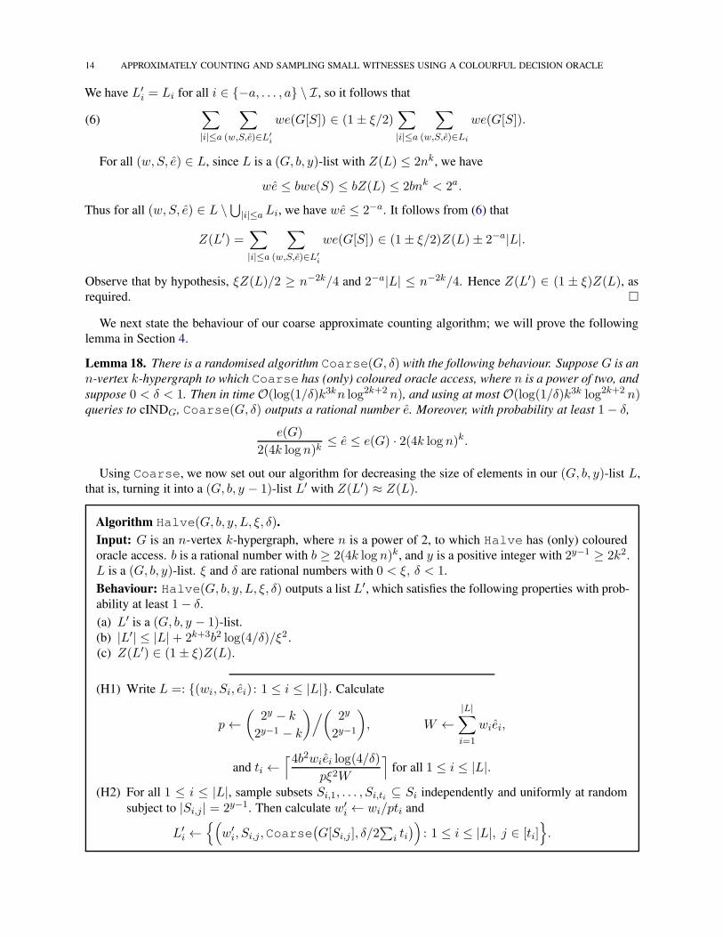
Using Coarse, we now set out our algorithm for decreasing the size of elements in our (G, b, y)-list L,
that is, turning it into a (G, b, y − 1)-list L′ with Z(L′) ≈ Z(L).
Algorithm Halve(G, b, y, L, ξ, δ).
Input: G is an n-vertex k-hypergraph, where n is a power of 2, to which Halve has (only) coloured
oracle access. b is a rational number with b ≥ 2(4k log n)k, and y is a positive integer with 2y−1 ≥ 2k2.
L is a (G, b, y)-list. ξ and δ are rational numbers with 0 < ξ, δ < 1.
Behaviour: Halve(G, b, y, L, ξ, δ) outputs a list L′, which satisfies the following properties with prob-
ability at least 1− δ.(a) L′ is a (G, b, y − 1)-list.
(b) |L′| ≤ |L|+ 2k+3b2 log(4/δ)/ξ2 .
(c) Z(L′) ∈ (1± ξ)Z(L).
(H1) Write L =: (wi, Si, ei) : 1 ≤ i ≤ |L|. Calculate
p←(
2y − k2y−1 − k
)/(2y
2y−1
), W ←
|L|∑
i=1
wiei,
and ti ←⌈4b2wiei log(4/δ)
pξ2W
⌉for all 1 ≤ i ≤ |L|.
(H2) For all 1 ≤ i ≤ |L|, sample subsets Si,1, . . . , Si,ti ⊆ Si independently and uniformly at random
subject to |Si,j| = 2y−1. Then calculate w′i ← wi/pti and
L′i ←
(w′i, Si,j,Coarse
(G[Si,j ], δ/2
∑i ti
)): 1 ≤ i ≤ |L|, j ∈ [ti]
.

APPROXIMATELY COUNTING AND SAMPLING SMALL WITNESSES USING A COLOURFUL DECISION ORACLE 15
(H3) Form L′ by concatenating the multisets L′i : 1 ≤ i ≤ |L| in arbitrary order and removing any
entries (w,S, e) with e = 0, and return L′.
Lemma 19. Halve(G, b, y, L, ξ, δ) behaves as claimed above. Moreover, writing
λ = |L|+ 2kb2 log(1/δ)
ξ2, T = λ log(λ/δ)k3k log2k+2 n,
Halve(G, b, y, L, ξ, δ) has running time O(nT ) and invokes cINDG at most O(T ) times.
Proof. Running time. The running time and oracle usage are both dominated by the invocations of Coarse
in step (H2). We first bound the number∑
i ti of such invocations. We have
(7)
|L|∑
i=1
ti ≤ |L|+|L|∑
i=1
4b2wiei log(4/δ)
pξ2W= |L|+ 4b2 log(4/δ)
pξ2.
Since 2y−1 ≥ 2k2, by a standard binomial coefficient bound (Lemma 14), we have p ≥ 2−k−1. Thus (7)
implies
(8)
|L|∑
i=1
ti ≤ |L|+2k+3b2 log(4/δ)
ξ2= Θ(λ).
By Lemma 18, writing T ′ = log(λ/δ)k3k log2k+2 2y−1, Coarse has running timeO(2y−1T ′) and invokes
cINDG O(T ′) times. Since L is a (G, b, y)-list, we have 2y−1 ≤ n and so the claimed bounds follow
from (8).
Correctness. Let E1 be the event that Z(L′) ∈ (1 ± ξ)Z(L), and let E2 be the event that every invocation
of Coarse in step (H2) succeeds. We will show that P(E1 ∩ E2) ≥ 1 − δ, and that properties (a)–(c) hold
whenever E1 ∩ E2 occurs.
Bounding P(E1 ∩ E2): To bound P(E1) below, we will apply Lemma 15. We first set up our notation
and show that the relevant assumptions hold. For all 1 ≤ i ≤ |L| and all j ∈ [ti], let
Xi,j := wie(G[Si,j ])/p, Mi := wieib/p,
µi := wie(G[Si]), µi := wiei.
For all i and j, it is clear that Xi,j ≥ 0. Moreover, since (wi, Si, ei) ∈ L, we have e(G[Si,j ]) ≤ e(G[Si]) ≤eib, so Xi,j ≤ Mi. Since L is a (G, b, y)-list, we have |Si| = 2y , so p is the probability that any given edge
in G[Si] survives in G[Si,j ]; thus µi = E(Xi,j). The Xi,j’s are independent, we have 0 ≤ µi ≤ µib, and we
have ⌈4bMi log(4/δ)
ξ2∑
ℓ µℓ
⌉=
⌈4b2wiei log(4/δ)
pξ2W
⌉= ti.
It therefore follows from Lemma 15 that with probability at least 1− δ/2,
(9)
|L|∑
i=1
ti∑
j=1
Xi,j
ti∈ (1± ξ)
|L|∑
i=1
µi.
Plugging our definitions in, we see (9) implies that Z(L′) ∈ (1± ξ)Z(L). Thus
(10) P(E1) ≥ 1− δ/2.By the correctness of Coarse (Lemma 18) and a union bound over all 1 ≤ i ≤ |L| and all j ∈ [ti], we
have P(E2) ≥ 1− δ/2. By a union bound with (10), we therefore have P(E1 ∩ E2) ≥ 1− δ as claimed.
Properties (a)–(c) hold: Suppose E1 ∩ E2 occurs. For every entry (w,S, e) of L′, w and e are positive
rational numbers and S ⊆ V (G) with |S| = 2y−1. Since E2 occurs and b ≥ 2(4k log n)k, by the correctness

16 APPROXIMATELY COUNTING AND SAMPLING SMALL WITNESSES USING A COLOURFUL DECISION ORACLE
of Coarse (Lemma 18) we have e/b ≤ e(G[S]) ≤ eb. Thus L is a (G, b, y−1)-list as required by property
(a). We have |L′| = ∑i ti, so (8) implies that property (b) holds. Finally, since E1 occurs, property (c)
holds. Thus properties (a)–(c) all hold whenever E1∩E2 occurs, which we have already shown happens with
probability at least 1− δ.
We now state our main algorithm.
Algorithm HelperCount(G, ε).
Input: G is an n-vertex k-hypergraph, where n is a power of 2. HelperCount has (only) coloured
oracle access to G, and ε is a rational number with 0 < ε < 1/2.
Behaviour: HelperCount(G, ε) outputs a rational number e such that with probability at least 2/3,
e ∈ (1± ε)e(G).
(A1) If ε < n−k, or if n ≤ 500, then return∑
Y⊆V (G), |Y |=k(1− cINDG(Y )).
(A2) If Coarse(G, δ) = 0, return 0. Otherwise, let
I ← log n− ⌈log(2k2)⌉, b← 2(4k log n)k,
ξ ← ε/4I, δ ← 1/3(2I + 1),
L←(
1, V (G),Coarse(G, δ)).
(A3) For i = 1 to I:
(We will maintain the invariant that L is a (G, b, log n− (i− 1))-list with Z(L) ∈ (1± ξ)2ie(G),and that |L| is suitably small (see proof of Lemma 20). Note that this is trivially satisfied at the
start of the loop.)
(A4) Update L← Halve(G, b, log n− (i− 1), L, ξ, δ).(This step turns L into a (G, b, log n− i)-list.)
(A5) Update L← Trim(G, b, log n− i, L, ξ, δ).(This step reduces the length of L.)
(A6) For each entry (w,S, e) ∈ L, calculate
eS ←∑
Y⊆S|Y |=k
(1− cINDG(Y )).
(A7) Output∑
(w,S,e)∈L weS .
Lemma 20. With probability at least 2/3, HelperCount(G, ε) outputs a rational number e ∈ (1±ε)e(G)as claimed above, has running timeO(ε−2k6kn log4k+7 n), and invokes cINDG at mostO(ε−2k6k log4k+7 n)times.
Proof. Correctness. Lemma 18 implies that correctness holds if HelperCount(G, ε) outputs on step
(A1) or (A2), so suppose that it does not. For all integers i ≥ 0, let π(i) be the statement that L satisfies the
following properties.
(i) L is a (G, b, log n− i)-list.
(ii) Z(L) ∈ (1± ξ)2ie(G).(iii) |L| ≤ 33k log(4nb) + 32b2 log(2/δ)/ξ2.
We will prove that with probability at least 2/3, π(i) holds at the end of the ith iteration of loop (A3) for
all i ∈ [I]. Suppose this is true: we will show that correctness follows. With probability at least 2/3, π(I)holds when we exit the loop. In this case, the final value of L satisfies Z(L) ∈ (1 ± ξ)2Ie(G) by (ii). We
have (1− ξ)2I ≥ 1− 2Iξ, and (1 + ξ)2I ≤ e2Iξ ≤ 1 + 4Iξ (since 4Iξ = ε < 1), so
Z(L) ∈ (1± 4Iξ)e(G) = (1± ε)e(G).

APPROXIMATELY COUNTING AND SAMPLING SMALL WITNESSES USING A COLOURFUL DECISION ORACLE 17
Moreover, in step (A6) we have eS = e(G[S]) for all (w,S, e) ∈ L, so Z(L) is the output.
It remains to prove that with probability at least 2/3, π(i) holds at the end of the ith iteration of loop (A3)
for all i ∈ [I]. Let E0 be the event that Coarse behaves correctly in step (A2); note that P(E0) ≥ 1 − δ by
the correctness of Coarse (Lemma 18). For all i ∈ [I], let Ei be the event that Halve behaves correctly
in the ith iteration of step (A4) and Trim behaves correctly in the ith iteration of step (A5). (If the input
restrictions of Halve or Trim are violated on the ith iteration, then Ei occurs automatically.) By correctness
of Halve and Trim (Lemmas 19 and 17), we have P(Ei | E0, . . . , Ei−1) ≥ 1− 2δ. Thus by a union bound
over all 0 ≤ i ≤ I , we have
P
( I⋂
i=0
Ei)≥ 1− (2I + 1)δ = 2/3.
It therefore suffices to show that when⋂
j Ej occurs, π(i) holds at the end of the ith iteration of loop (A3)
for all i ∈ [I].At the start of the first iteration of loop (A3), when i = 1, L is a (G, b, log n)-list since E0 occurs,
Z(L) = e(G), and |L| = 1. Thus π(0) holds. Let i ∈ [I], and suppose that π(i− 1) holds at the start of the
ith iteration of loop (A3). Let Li be the value of L at the start of the ith iteration, let L′i be the value of L
after executing step (A4), and let Li+1 be the value of L after executing step (A5).
By property (i), Li is a (G, b, log n − (i − 1))-list, where by our choice of I we have 2log n−i ≥ 2k2.
Since Ei occurs, it follows by the correctness of Halve (Lemma 19) that L′i is a (G, b, log n− i)-list with
Z(L′i) ∈ (1± ξ)Z(Li),
|L′i| ≤ |Li|+ 2k+3b2 log(4/δ)/ξ2.
We next show that 1/2 ≤ Z(L′i) ≤ 2nk, that |L′
i| ≤ n11k, and that ξ ≥ n−2k, as required by Trim. Since
property (ii) holds for Z(Li), we have Z(L′i) ∈ (1±ξ)2i+1e(G) ⊆ (1±ε)e(G). Since HelperCount(G, ε)
did not halt at (A2), we have 1 ≤ e(G) ≤ nk; since ε < 1/2, it follows that 1/2 ≤ Z(L′i) ≤ 2nk. Since
HelperCount(G, ε) did not halt at (A1), we have n ≥ 500 and hence n ≥ 50 log n. We also have
ε ≥ n−k and k ≤ n. Hence:
b2 ≤ n4k; 2k ≤ nk; log(4/δ) ≤ log(24 log n) ≤ n;log(4nb) ≤ 6k log n ≤ n2; 1/ξ2 ≤ 16(log n)2n2k ≤ n4k.
Since property (iii) holds for Li, it follows that
|L′i| ≤ 33k log(4nb) + 40 · 2kb2 log(4/δ)/ξ2 ≤ 33n3 + 40n9k+1 ≤ n10k.
We have therefore shown that L′i and ξ satisfy the input restrictions of Trim. Since Ei occurs, by the
correctness of Trim (Lemma 17) it follows that Li+1 is a (G, b, log n− i)-list with
Z(Li+1) ∈ (1± ξ)Z(L′i) ⊆ (1± ξ)2Z(Li) ⊆ (1± ξ)2(i+1)e(G),
|Li+1| ≤ 33k log(4nb) + 32b2 log(2/δ)/ξ2.
Thus properties (i)–(iii) hold for Li+1, as required.
Running time and oracle queries. If step (A1) is executed, so that ε < n−k or n ≤ 500, then the algorithm
runs in time O(nk) = O(ε−1) and uses O(nk) = O(ε−1) oracle queries, so our claimed bounds hold.
Suppose instead step (A1) is not executed, so that ε ≥ n−k. Recall that⋂
i Ei holds with probability at least
2/3. Suppose this occurs. The bottleneck in both running time and oracle invocations is then step (A4).
For legibility, we give the time and oracle requirements of the other steps in the following table, giving
justifications in the paragraph below. We write Λ = 33k log(4nb) + 32b2 log(2/δ)/ξ2 for the upper bound
on |L| in property (iii) of our invariant π.

18 APPROXIMATELY COUNTING AND SAMPLING SMALL WITNESSES USING A COLOURFUL DECISION ORACLE
Step number Running time Oracle calls
(A1) O(1) None
(A2) O(k3kn log2k+2 n log(1/δ)
)O(k3k log2k+2 n log(1/δ)
)
(A3) O(I) None
(A5) O(I(Λ+ 2kb2ξ−2 log(1/δ)
)k2 log n
)None
(A6) O(Λ(4k2)k) O(Λ(4k2)k)(A7) O(Λ) None
For step (A1), we use the fact that ε ≥ n−k and so the conditional does not trigger. For step (A2), we use
the fact that n is a power of 2 (so computing log n is easy) and the time bounds on Coarse (Lemma 18).
For step (A5), we first observe that the step is executed I times. We then apply the time bounds on Trim
(Lemma 17), together with property (iii) and the fact that Halve adds at most 2k+3b2ξ−2 log(4/δ) to the
length of L (see Lemma 19). (Note that k log(nb/δ) = O(k2 log n).) For step (A6), we use the fact that
after the loop of (A3), L is a (G, b, log n− I)-list, so each entry (w,S, e) of L has |S| = 2log n−I ≤ 4k2.
We now consider step (A4), which is executed I times. From the time bounds of Halve (Lemma 19), it
follows that the total running time of step (A4) is O(nT ) and the total number of oracle accesses is O(T )times, where
T = O(Iλ log(λ/δ)k3k log2k+2 n
), λ = Λ+ 2kb2ξ−2 log(1/δ).
This clearly dominates everything in the table. Observe that Λ = O(2kb2ξ−2 log(1/δ)), so λ = O(2kb2ξ−2 log(1/δ))also. Since ε ≥ n−k,
log(λ/δ) = O(k + k log(k log n) + log I + log(1/ε) + log(1/δ)
)= O(k log n).
Thus
T = O(I2kb2ξ−2 log(1/δ)k3k+1 log2k+3 n
)
= O(log n · 2k · (k log n)2k · ε−2 log2 n · log log n · k3k+1 log2k+3 n
)
= O(ε−2k6k log4k+7 n
),
and the claimed bounds follow.
We now prove Theorem 1.
Theorem 1 (restated). There is a randomised algorithm Count(G, ε, δ) with the following behaviour. Sup-
pose G is an n-vertex k-hypergraph, and that Count has coloured oracle access to G. Suppose ε and δare rational with 0 < ε, δ < 1. Then, writing T = log(1/δ)ε−2k6k log4k+7 n: in time O(nT ), and using at
most O(T ) queries to cINDG, Count(G, ε, δ) outputs a rational number e. With probability at least 1− δ,we have e ∈ (1± ε)e(G).Proof. To evaluate Count(G, ε, δ), we first make n into a power of two by adding at most n isolated vertices
toG; note that this does not impede the evaluation of cINDG. We then run HelperCount(G,minε, 1/3)a total of 36⌈ln(2/δ)⌉ times and return the median result e. If some invocation of HelperCount(G,minε, 1/3)takes more than Θ(ε−2k6kn log4k+7 n) time, or invokes cINDG more than Θ(ε−2k6k log4k+7 n) times, we
halt execution and consider the output to be −1.
It is immediate that this algorithm satisfies our stated time bounds. Moreover, e ∈ (1 ± ε)e(G) unless
at least half our invocations of HelperCount fail. The number of such failures is dominated above by a
binomial variable N with mean 12⌈ln(2/δ)⌉, so by a standard Chernoff bound (namely Lemma 13(i)) we
have
P(e /∈ (1± ε)e(G)
)≤ P
(N ≥ 18⌈ln(2/δ)⌉
)≤ P
(∣∣N − E(N)∣∣ ≥ 1
2E(N)
)≤ 2e−⌈ln(2/δ)⌉ ≤ δ,
as required.

APPROXIMATELY COUNTING AND SAMPLING SMALL WITNESSES USING A COLOURFUL DECISION ORACLE 19
4. COARSE APPROXIMATE COUNTING
In this section, we prove Lemma 18. Throughout, we fix the input graphG to be an n-vertex k-hypergraph
to which we have (only) coloured oracle access, where n is a power of two.
4.1. Sketch proof. The heart of our algorithm will be a subroutine to solve the following simpler “gap-
version” of the problem. Given a k-partite k-hypergraph G and a guess M ≥ 0, we ask: Does G have more
than M edges? We wish to answer correctly with high probability provided that either G has at least Medges, or G has significantly fewer than M edges, namely at most γM edges with γ = 1/(23k+1k2k logk n).Suppose we can solve this problem probabilistically, perhaps outputting Yes with probability at least 1/50if e(G) ≥ M (which we call completeness) and outputting Yes with probability at most 1/100 if e(G) ≤γM (which we call soundness). We then apply probability amplification to substantially reduce the failure
probability, and use binary search to find the least M such that our output is Yes— with high probability,
this will approximate e(G) when our input k-hypergraph is k-partite. We then generalise our algorithm to
arbitrary inputs using random colour-coding. These parts of the algorithm are fairly standard, so in this
sketch proof we will only solve the gap-problem. (We implement this sketch below as the VerifyGuess
algorithm.)
Let G be a k-partite k-hypergraph with vertex classes X1, . . . ,Xk . The basic idea of the algorithm is
to randomly remove vertices from G to form a new graph H in such a way that each edge survives with
probability roughly 1/M , and then query the coloured independence oracle and output Yes if and only if
at least one edge remains. If G has at most γM edges, then a union bound implies we are likely to output
No (soundness); if G has at least M edges, then in expectation at least one edge survives the removal, so
we hope to output Yes (completeness). Unfortunately, the number of edges remaining in H need not be
concentrated around its expectation — for example, if every edge of G is incident to a single vertex v — so
we must be very careful if this hope is to be realised.
Suppose for the moment that k = 2, so that G is a bipartite graph with vertex classes X1 and X2. Then
we will form X ′1 ⊆ X1 by including each vertex independently with probability p1, and X ′
2 ⊆ X2 by
including each vertex independently with probability p2. Each edge survives with probability p1p2, so we
require p1p2 ≤ 1/M to ensure soundness. To ensure completeness, we would then like to choose p1 and p2such that G[X ′
1,X′2] is likely to contain an edge whenever e(G) ≥M .
To see that such a pair (p1, p2) exists, we first partition the vertices in X1 according to their degree: For
1 ≤ d ≤ log n, let Xd1 be the set of vertices v with 2d−1 ≤ d(v) < 2d. By the pigeonhole principle,
there exists some D such that XD1 is incident to at least e(G)/ log n edges. Then we take p1 = 2D/M
and p2 = 1/2D . We certainly have p1p2 ≤ 1/M . Suppose e(G) ≥ M . Since XD1 is incident to at
least e(G)/ log n edges, we have |XD1 | ≥M/2D log n, so with reasonable probability X ′
1 contains a vertex
v1 ∈ XD1 . Then v1 has degree roughly 2D in X2, so again with reasonable probability X ′
2 contains a vertex
adjacent to it.
There is one remaining obstacle: Since we only have coloured oracle access to G, we do not know what
D is! Fortunately, since there are only O(log n) possibilities, we can simply try them all in turn, and output
Yes if any one of them yields a pair X ′1, X
′2 such that G[X ′
1,X′2] contains an edge. (It is not hard to tune the
parameters so that this doesn’t affect soundness.) This is essentially the argument used by Beame et al. [6].
When we try to generalise this approach to k-hypergraphs, we hit a problem. For illustration, take k = 3and suppose e(G) ≥ M . Then we wish to guess a vector (p1, p2, p3) such that p1p2p3 ≤ 1/M and, with
reasonable probability, G[X ′1,X
′2,X
′3] contains an edge. As in the k = 2 case, we can guess an integer
0 ≤ D ≤ 2 log n such that a large proportion of G’s edges are incident to a vertex in X1 of degree roughly
2D. Also as in the k = 2 case, if we take p1 = 2D/M then it is reasonably likely that X ′1 will contain a
vertex of degree roughly 2D, say v1. But we cannot iterate this process — the structure of G[v1,X2,X3],and hence the “correct” value of p2, depends very heavily on v1. So for example, when we test the two
guesses (2D/M, 1/2D , 1) and (2D/M, 1, 1/2D), we wish to ensure that the value of v1 is the same in each
test. This is the reason for step (C1) in the following algorithm; it is important that we do not choose new
random subsets of X1, . . . ,Xk independently with each iteration of step (C2).

20 APPROXIMATELY COUNTING AND SAMPLING SMALL WITNESSES USING A COLOURFUL DECISION ORACLE
Algorithm VerifyGuess(G,M,X1, . . . ,Xk).
Input: G is an n-vertex k-hypergraph to which VerifyGuess has (only) coloured oracle access. nand M are positive powers of two, and X1, . . . ,Xk ⊆ V (G) are disjoint.
Behaviour: Let pout = (8k log n)−k.
Completeness: If e(G[X1, . . . ,Xk]) ≥ M , then VerifyGuess outputs Yes with probability at least
pout.Soundness: If e(G[X1, . . . ,Xk]) < M · pout/2(k log n)k, then VerifyGuess outputs Yes with
probability at most pout/2.
(C1) For each i ∈ [k] and each 0 ≤ j ≤ k log n, construct a subset Yi,j of Xi by including each vertex
independently with probability 1/2j . Construct the finite set A of all tuples (a1, . . . , ak) with
0 ≤ a1, . . . , ak ≤ k log n and a1 + · · ·+ ak ≥ logM .
(C2) For each tuple (a1, . . . , ak) ∈ A: If cINDG(Y1,a1 , . . . , Yk,ak) = 0, then halt and output Yes.
(C3) We have not halted yet, but do so now and output No.
4.2. Solving the gap problem.
Lemma 21. VerifyGuessbehaves as stated, runs in timeO(nkk logk n), and makes at mostO(kk logk n)oracle queries.
Proof. Let G,M,X1, . . . ,Xk be the input for VerifyGuess, and let H = G[X1, . . . ,Xk]. For nota-
tional convenience, we denote the gap in the soundness case by γ, that is, we set γ := pout/2(k log n)k =
1/23k+1k2k log2k n.
Running time and oracle queries. Step (C1) takes O(nk log n+ kk logk n) time and no oracle queries; step
(C2) takes O(kk logk n) time and O(kk logk n) oracle queries; and step (C3) takes O(1) time and no oracle
queries. The claimed bounds follow, and it remains to prove that the soundness and completeness properties
hold.
Soundness. We next prove soundness, as this is the easier part of proving correctness. So suppose e(H) ≤γM . Let (a1, . . . , ak) ∈ A, and let H ′ ⊆ H denote the random induced subgraph G[Y1,a1 , . . . , Yk,ak ]. Then
for all e ∈ E(H), we have
P(e ∈ E(H ′)) =k∏
j=1
2−aj ≤ 1
M≤ γ
e(H)≤ pout
2|A|e(H).
By a union bound over all e ∈ E(H) and all (a1, . . . , ak) ∈ A, it follows that the probability that
VerifyGuess outputs Yes is at most pout/2. This establishes the soundness of the algorithm, so it
remains to prove completeness.
Completeness. Suppose now that e(H) ≥M holds. We must prove that VerifyGuess outputs Yes with
probability at least pout. It suffices to show that with probability at least pout, there is at least one setting of
the vector (a1, . . . , ak) ∈ A such that G[Y1,a1 , . . . , Yk,ak ] contains at least one edge.
We will define this setting iteratively. First, with reasonable probability, we will find an integer a1 and a
vertex v1 ∈ Y1,a1 such that G[v1,X2, . . . ,Xk] contains roughly 2−a1e(H) edges. In the process, we expose
Y1,a1 . We then, again with reasonable probability, find an integer a2 and a vertex v2 ∈ Y2,a2 such that
G[v1, v2,X3, . . . ,Xk] contains roughly 2−a1−a2e(H) edges. Continuing in this vein, we eventually find
(a1, . . . , ak) ∈ A and vertices vi ∈ Yi,ai such that v1, . . . , vk is an edge in G[Y1,a1 , . . . , Yk,ak ], proving
the result.
More formally, for all i ∈ [k], let Ei be the event that there exist 0 ≤ a1, . . . , ai ≤ k log n and v1, . . . , vi ∈V (H) such that:

APPROXIMATELY COUNTING AND SAMPLING SMALL WITNESSES USING A COLOURFUL DECISION ORACLE 21
(a) for all j ∈ [i], vj ∈ Yj,aj ;
(b) we have dH(v1, . . . , vi) ≥ e(H)/∏i
j=1 2aj .
We make the following Claim: P(E1) ≥ 1/(8k log n) and, for all 2 ≤ i ≤ k, P(Ei | Ei−1) ≥ 1/(8k log n).Proof of Lemma 21 from Claim: Suppose Ek occurs, and let a1, . . . , ak and v1, . . . , vk be as in the
definition of Ek. By (b), dH(v1, . . . , vk) > 0, so v1, . . . , vk is an edge in H; it follows by (a) that it is also
an edge in G[Y1,a1 , . . . , Yk,ak ]. Also by (b), since dH(v1, . . . , vk) = 1, we have∏k
j=1 2aj ≥ e(H) ≥M , so
a1 + · · · + ak ≥ logM . Thus (a1, . . . , ak) ∈ A, so whenever Ek occurs, VerifyGuess outputs Yes on
reaching (a1, . . . , ak) in step (C2). By the Claim, we have
P(Ek) = P(E1)k∏
j=2
P(Ej | E1, . . . , Ej−1) = P(E1)k∏
j=2
P(Ej | Ej−1) ≥ 1/(8k log n)k = pout,
so completeness follows and hence so does the lemma statement.
Proof of Claim: We first prove the claim for E1. We will choose a1 depending on the degree distribution
of vertices in X1. For all integers 1 ≤ d ≤ k log n, let
Xd1 := v ∈ X1 : 2
d−1 ≤ dH(v) < 2d
be the set of vertices in X1 with degree roughly 2d. Every edge in H is incident to exactly one vertex in
exactly one set Xd1 , so there exists D such that XD
1 is incident to at least e(H)/k log n edges of H . We take
a1 := ⌈log e(H)⌉ −D + 1. Note that 0 ≤ a1 ≤ k log n, since XD1 6= ∅ and so e(H) ≥ 2D−1.
We would like to take v1 ∈ Y1,a1 ∩XD1 , so we next bound the probability that this set is non-empty. We
have
P(XD1 ∩ Y1,a1 6= ∅) = 1− (1− 2−a1)|X
D1 | ≥ 1− exp(−2−a1 |XD
1 |).
Since every vertex in XD1 has degree at most 2D , by the definition of D we have 2D|XD
1 | ≥ e(H)/(k log n).Moreover, we have a1 ≤ log e(H)−D + 2. It follows that
P(XD1 ∩ Y1,a1 6= ∅) ≥ 1− exp
(−2D−2
e(H)· e(H)
k2D log n
)= 1− exp
(− 1
4k log n
)≥ 1
8k log n.
Suppose XD1 ∩ Y1,a1 6= ∅, and take v1 ∈ XD
1 ∩ Y1,a1 . Then v1 certainly satisfies (a), and by the definitions
of a1 and XD1 we have e(H)/2a1 ≤ 2D−1 ≤ dH(v1), so v1 also satisfies (b). We have therefore shown
P(E1) ≥ 1/(8k log n) as required.
Now let 2 ≤ i ≤ k. The argument is similar, but we include it explicitly for the benefit of the reader. We
first expose Y1,a1 , . . . , Yi−1,ai−1: Let F be a possible filtration of these variables consistent with Ei−1, and
let a1, . . . , ai−1 and v1, . . . , vi−1 be as in the definition of Ei−1. It then suffices to show that P(Ei | F) ≥1/(8k log n).
Similarly to the i = 1 case, for all integers 1 ≤ d ≤ k log n, let
Xdi := v ∈ Xi : 2
d−1 ≤ dH(v1, . . . , vi−1, v) < 2d.
Every edge in H[v1, . . . , vi−1,Xi, . . . ,Xk] is incident to exactly one vertex in exactly one set Xdi , so there
existsDi such thatXDi
i is incident to at least dH(v1, . . . , vi−1)/k log n edges ofH[v1, . . . , vi−1,Xi, . . . ,Xk].We take ai := ⌈log dH(v1, . . . , vi−1)⌉ −Di + 1; note that 0 ≤ ai ≤ k log n.
As in the i = 1 case, we would like to take vi ∈ Yi,ai ∩XDi
i , so we next bound the probability that this
set is non-empty. Since every vertex v ∈ XDi
i satisfies dH(v1, . . . , vi−1, v) ≤ 2Di , we have 2Di |XDi
i | ≥

22 APPROXIMATELY COUNTING AND SAMPLING SMALL WITNESSES USING A COLOURFUL DECISION ORACLE
dH(v1, . . . , vi−1)/k log n. It follows that
P(XDi
i ∩ Yi,ai 6= ∅ | F) = 1− (1− 2−ai)|XDii | ≥ 1− exp(−2−ai |XDi
i |)
≥ 1− exp(− 2Di−2
dH(v1, . . . , vi−1)· dH(v1, . . . , vi−1)
k2Di log n
)
= 1− exp(− 1
4k log n
)≥ 1
8k log n.
Suppose XDi
i ∩ Yi,ai 6= ∅, and take vi ∈ XDi
i ∩ Yi,ai . Then vi certainly satisfies (a). By the definitions of aiand XDi
i , and the fact that v1, . . . , vi−1 satisfy (b), we have
e(H)/
i∏
j=1
2aj ≤ dH(v1, . . . , vi−1)/2ai ≤ 2Di−1 ≤ dH(v1, . . . , vi).
Thus (b) is satisfied, and we have shown P(Ei | F) ≥ 1/(8k log n) as required.
4.3. Proving Lemma 18. We next turn VerifyGuess into a crude approximation algorithm for k-partite
k-hypergraphs in the natural way.
Algorithm ColourCoarse(G,X1, . . . ,Xk).
Input: G is an n-vertex k-hypergraph, where n is a power of two, to which ColourCoarse has
coloured oracle access (only). X1, . . . ,Xk form a partition of V (G).
Behaviour: Let b := (4k log n)k. Then ColourCoarse (G) outputs a non-negative integer m such
that, with probability at least 2/3, m/b ≤ e(G[X1, . . . ,Xk]) ≤ mb.
(D1) Set pout := (8k log n)−k and N := ⌈48 ln(6k log n)/pout⌉.(D2) For each M in 1, 2, 4, 8, . . . , nk: Execute VerifyGuess (G,M,X1, . . . ,Xk) a total of N
times, and let SM ∈ 0, . . . , N be the number of executions that returned Yes. (Naturally we
use independent randomness for each value of M .)
(D3) If cINDG(X1, . . . ,Xk) = 1, let m = 0. Otherwise, if there exists M such that SM ≥ 34poutN , let
m be the least such M . Otherwise, let m = nk. Output m(pout/2k
k logk n)1/2
.
Lemma 22. ColourCoarsebehaves as stated, runs in timeO((8k log n)2k+2n), and requiresO((8k log n)2k+2)oracle queries.
Proof. LetG and X1, . . . ,Xk be the inputs, so that G is an n-vertex k-hypergraph and X1, . . . ,Xk partition
V (G).Running time and oracle queries. Observe N = O((8k log n)k+1). ColourCoarse just executes
VerifyGuess at most O(log(nk)N) times. By Lemma 21, each execution takes O(nkk logk n) time and
makes O(kk logk n) oracle queries. Thus the claimed bounds on the running time and number of oracle
queries of ColourCoarse follow.
Correctness. Let M ∈ 1, 2, 4, 8, . . . , nk, and let H = G[X1, . . . ,Xk]. For this fixed M , the algo-
rithm invokes VerifyGuessN times, so the random variable SM is the sum of N independent indicator
variables. By a standard Chernoff bound (Lemma 13(i) taking ε = 1/4),
P(|SM − E(SM )| ≥ E(SM )/4
)≤ 2 exp
(− 1
48E(SM ))
(11)
If e(H) ≥ M , then the completeness of VerifyGuess implies E(SM) ≥ Npout. Thus (11) and our
choice of N imply that
P(SM < 3
4Npout)≤ 2 exp
(− 1
48Npout)≤ 1/(3k log n).

APPROXIMATELY COUNTING AND SAMPLING SMALL WITNESSES USING A COLOURFUL DECISION ORACLE 23
Similarly, if M > 2(k log n)k · e(H)/pout, then the soundness of VerifyGuess implies E(SM ) ≤Npout/2. But then (11) implies that
P(SM > 3
4Npout)≤ P
(SM > 5
4E(SM))≤ 2 exp
(− 1
48Npout)≤ 1/(3k log n).
Finally, we perform a union bound over all M ∈ 1, 2, 4, 8, . . . , nk that satisfy either M ≤ e(H) or
M ≥ 2kk logk n ·e(H)/pout. (Note that no value of M satisfies both inequalities.) There are at most k log nsuch M ’s, so with probability at least 2/3, we see SM < 3Npout/4 for all M ≤ e(H) and SM > 3Npout/4
for all M ≥ 2kk logk n · e(H)/pout. By the definition of m, it follows that in this case
pout
2kk logk nm ≤ e(H) ≤ m.
Hence, writing x = m(pout/2kk logk n)1/2 for the output of ColourCoarse,
x
√pout
2kk logk n≤ e(H) ≤ x
/√pout
2kk logk n.
Since pout = 1/(8k log n)k, the output of ColourCoarse approximates e(H) up to a factor of (4k log n)k
as required.
We now combine our algorithm for coarsely approximately counting edges in k-partite k-hypergraphs
with colour-coding to obtain an algorithm for general k-hypergraphs.
Algorithm HelperCoarse(G).
Input: G is an n-vertex k-hypergraph, where n is a power of two, to which HelperCoarse has
coloured oracle access (only).
Behaviour: HelperCoarse(G) outputs a non-negative integer e which, with probability at least 2/3,
satisfies e/2(4k log n)k ≤ e(G) ≤ e · 2(4k log n)k.
(E1) Let t = 3e2k , and let T = ⌈72 ln t⌉+ 3.
(E2) For each i ∈ [t]:(E3) Sample a uniformly random function ci : V (G) → [k], which yields a random k-partition
X1, . . . ,Xk of V (G).(E4) Execute ColourCoarse(G,X1, . . . ,Xk) exactly T times and letMi be the median output
produced by these executions.
(E3) Output kk
tk!
∑ti=1Mi.
Lemma 23. HelperCoarse behaves as stated, runs in time O(k3kn log2k+2 n), and requires
O(k3k log2k+2 n) oracle queries.
Proof. Let G be an n-vertex k-hypergraph input for HelperCoarse.
Running time and oracle queries. It is clear that the bottleneck in both the running time and the number
of oracle queries is the T t total invocations of ColourCoarse. Recall from Lemma 22 that each such
invocation runs in time O(n(8k log n)2k+2) and requires O((8k log n)2k+2) oracle queries. Since t =O(e2k) and T = O(k), the claimed bounds follow.
Correctness. Let b := (4k log n)k be the approximation ratio of ColourCoarse. For all i ∈ [t], let
Gi = G[c−1i (1), . . . , c−1
i (k)] be the ith hypergraph we consider, and let mi = e(Gi). Let xi,j be the output
of the jth call to ColourCoarse in evaluating Mi, and let Ei,j be the event that xi,j/b ≤ mi ≤ xi,jb.Note that the Ei,j’s are independent conditioned on ci, and that the correctness of ColourCoarse
(Lemma 22) implies that P(Ei,j) ≥ 2/3 for all j ∈ [T ]. Moreover, for all i ∈ [t], if at least half the Ei,j’s

24 APPROXIMATELY COUNTING AND SAMPLING SMALL WITNESSES USING A COLOURFUL DECISION ORACLE
occur, then Mi/b ≤ mi ≤ bMi. Thus by a Chernoff bound (Lemma 13(i) applied with ε = 1/4 and
µ = 2T/3), we have
P(1bMi ≤ mi ≤ bMi | ci) ≥ 1− 2e−T/72 ≥ 1− 2e− ln t−3 > 1− 1/(6t).
It follows by a union bound that, with probability at least 5/6, Mi/b ≤ mi ≤ bMi for all i ∈ [t].Now observe that E(
∑imi) = t(k!/kk)e(G), and that eachmi lies in [0, e(G)]. It follows by Hoeffding’s
inequality (Lemma 11) that
P
(∣∣∣kk
tk!
∑
i
mi − e(G)∣∣∣ >
1
2e(G)
)= P
(∣∣∣∑
i
mi −tk! · e(G)
kk
∣∣∣ >tk!
2kke(G)
)
≤ 2 exp
(−2
( tk!kke(G)
)2/te(G)2
)= 2exp
(−2t(k!/kk)2
).
By Stirling’s formula and our definition of t, it follows that
P
(∣∣∣kk
tk!
∑
i
mi − e(G)∣∣∣ >
1
2e(G)
)≤ 2 exp
(−te−2k
)≤ 1/6.
Thus with probability at least 5/6, we have e(G)/2 ≤ kk
tk!
∑imi ≤ 2e(G).
It now follows by a union bound that with probability at least 2/3, 12b · e(G) ≤ kk
tk!
∑iMi ≤ 2b · e(G) as
required.
Lemma 18 now follows via the usual probability amplification argument.
Lemma 18 (restated). There is a randomised algorithm Coarse(G, δ) with the following behaviour. Sup-
pose G is an n-vertex k-hypergraph to which Coarse has (only) coloured oracle access, where n is a
power of two, and suppose 0 < δ < 1. Then in time O(log(1/δ)k3kn log2k+2 n), and using at most
O(log(1/δ)k3k log2k+2 n) queries to cINDG, Coarse(G, δ) outputs a rational number e. Moreover, with
probability at least 1− δ,e(G)
2(4k log n)k≤ e ≤ e(G) · 2(4k log n)k.
Proof. Given G and δ > 0, we simply invoke HelperCoarse(G) a total of T := ⌈36 ln(2/δ)⌉ times
and return the median output. By the correctness of HelperCoarse (Lemma 23), each invocation returns
a valid approximation of e(G) with probability at least 2/3, and if at least T/2 invocations return valid
approximations then the median is also a valid approximation. It follows by Chernoff bounds (Lemma 13(i)
with ε = 1/2 and µ = T/3) that we output a valid approximation with probability at least 1 − 2e−T/36 ≥1− δ, as required, and our bounds on running time and oracle usage are immediate from Lemma 23.
5. APPROXIMATELY UNIFORM SAMPLING
In this section we demonstrate that we can use our approximate counting algorithm to sample an edge
almost uniformly at random, proving Theorem 2. The core of our algorithm is the following subroutine.
Algorithm HelperSample(G, ε).
Input: G is an n-vertex k-hypergraph containing at least one edge, where n is a power of two, to which
HelperCoarse has coloured oracle access (only). 0 < ε < 1/2 is a rational number.
Behaviour: With probability at least 1− ε/nk, HelperSample(G, ε) outputs a sample from a distri-
bution U on E(G) such that, for all e ∈ E(G), U(e) ∈ (1± ε)/e(G).
(S1) If ε ≤ n−k, then enumerate the edges ofG using(nk
)invocations of cINDG and return a uniformly-
sampled edge.
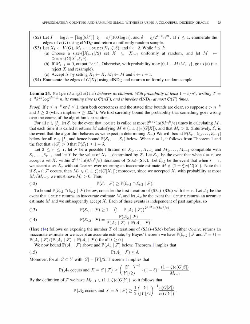
APPROXIMATELY COUNTING AND SAMPLING SMALL WITNESSES USING A COLOURFUL DECISION ORACLE 25
(S2) Let I = log n − ⌈log(8k2)⌉, ξ = ε/(100 log n), and δ = ξ/2k+8n2k. If I ≤ 1, enumerate the
edges of e(G) using cINDG and return a uniformly random sample.
(S3) Let X1 ← V (G), M1 ← Count(X1, ξ, δ), and i← 2. While i ≤ I:
(a) Choose a size-(|Xi−1|/2) set X ⊆ Xi−1 uniformly at random, and let M ←Count(G[X], ξ, δ).
(b) If Mi−1 = 0, output Fail. Otherwise, with probability max0, 1−M/Mi−1, go to (a) (i.e.
reject X and resample).
(c) Accept X by setting Xi ← X, Mi ←M and i← i+ 1.
(S4) Enumerate the edges of G[XI ] using cINDG and return a uniformly random sample.
Lemma 24. HelperSample(G, ε) behaves as claimed. With probability at least 1 − ε/nk, writing T =
ε−2k7k log4k+11 n, its running time is O(nT ), and it invokes cINDG at most O(T ) times.
Proof. If ε ≤ n−k or I ≤ 1, then both correctness and the stated time bounds are clear, so suppose ε > n−k
and I ≥ 2 (which implies n ≥ 32k2). We first carefully bound the probability that something goes wrong
over the course of the algorithm’s execution.
For all r ∈ [I], let Er be the event that Count is called at most 2k+2 ln(8Ink/ε) times in calculating Mr ,
that each time it is called it returns M satisfying M ∈ (1 ± ξ)e(G[X]), and that Mr > 0. (Intuitively, Er is
the event that the algorithm behaves as we expect in determining Xr.) We will bound P(Er | E1, . . . , Er−1)below for all r ∈ [I], and hence bound P(E1, . . . , Er) below. When r = 1, it follows from Theorem 1 and
the fact that e(G) > 0 that P(E1) ≥ 1− δ.Let 2 ≤ r ≤ I , let F be a possible filtration of X1, . . . ,Xr−1 and M1, . . . ,Mr−1 compatible with
E1, . . . , Er−1, and let Y be the value of Xr−1 determined by F . Let Er,1 be the event that when i = r, we
accept a set Xr within 2k+2 ln(8Ink/ε) iterations of (S3a)–(S3c). Let Er,2 be the event that when i = r,
we accept a set Xr without Count ever returning an inaccurate estimate M /∈ (1 ± ξ)e(G[X]). Note that
if Er,2 ∩ F occurs, then Mr ∈ (1 ± ξ)e(G[Xr ]); moreover, since we accepted Xr with probability at most
Mr/Mr−1, we must have Mr > 0. Thus
(12) P(Er | F) ≥ P(Er,1 ∩ Er,2 | F).To bound P(Er,1 ∩ Er,2 | F) below, consider the first iteration of (S3a)–(S3c) with i = r. Let A1 be the
event that Count returns an inaccurate estimate M , and let A2 be the event that Count returns an accurate
estimate M and we subsequently accept X. Each of these events is independent of past samples, so
P(Er,1 | F) ≥ 1−(1− P(A2 | F)
)2k+2 ln(8Ink/ε),(13)
P(Er,2 | F) =P(A2 | F)
P(A2 | F) + P(A1 | F).(14)
(Here (14) follows on exposing the number T of iterations of (S3a)–(S3c) before either Count returns an
inaccurate estimate or we accept an accurate estimate; by Bayes’ theorem we have P(Er,2 | F and T = t) =P(A2 | F)/(P(A2 | F) + P(A1 | F)) for all t ≥ 0.)
We now bound P(A1 | F) above and P(A2 | F) below. Theorem 1 implies that
(15) P(A1 | F) ≤ δ.Moreover, for all S ⊂ Y with |S| = |Y |/2, Theorem 1 implies that
P(A2 occurs and X = S | F
)≥
( |Y ||Y |/2
)−1
· (1− δ) · (1− ξ)e(G[S])Mr−1
.
By the definition of F we have Mr−1 ∈ (1± ξ)e(G[Y ]), so it follows that
P(A2 occurs and X = S | F
)≥ 1
2
( |Y ||Y |/2
)−1 e(G[S])
e(G[Y ]).

26 APPROXIMATELY COUNTING AND SAMPLING SMALL WITNESSES USING A COLOURFUL DECISION ORACLE
On summing both sides over S, since each edge of G[Y ] appears in exactly( |Y |−k|Y |/2−k
)sets S ⊂ Y with
|S| = |Y |/2, we obtain
P(A2 | F) ≥1
2
( |Y ||Y |/2
)−1( |Y | − k|Y |/2− k
).
Since r ≤ I , we have |Y | ≥ n/2I−1 ≥ 4k2, so by Lemma 14 it follows that P(A2 | F) ≥ 2−k−2. It
therefore follows from (13), (14) and (15) that
P(Er,1 | F) ≥ 1− (1− 2−k−2)2k+2 ln(8Ink/ε) ≥ 1− e− ln(8Ink/ε) = 1− ε/8Ink,
P(Er,2 | F) ≥ 2−k−2/(2−k−2 + δ) ≥ 1− 2k+2δ ≥ 1− ε/8Ink.
By (12), it follows that P(Er | F) ≥ 1− ε/4Ink for all r ∈ [I]. Thus
(16) P(E1, . . . , EI) ≥ 1− ε/4nk.With (16) in hand, we are now ready to proceed with the main proof.
Running time and oracle queries. Since |XI | = n/2I−1 ≤ 32k2 by our choice of I , the bottleneck
in the running time is the invocations of Count in (S3b). By Theorem 1, each invocation takes time
O(log(1/δ)ξ−2k6kn log4k+7 n) and requiresO(log(1/δ)ξ−2k6k log4k+7 n) invocations of the oracle. Since
1/ξ = O(log n/ε), log(1/δ) = O(k log n + log(1/ε)) and 1/ε = O(nk), each invocation takes time
O(ε−2k6k+1n log4k+10 n) and requires O(ε−2k6k+1 log4k+10 n) oracle invocations. By (16), with probabil-
ity at least 1 − ε/nk, there are at most 2k+2 ln(8Ink/ε) = O(k2k log n) such invocations, so the claimed
bounds follow.
Correctness. Let F be the output of HelperSample(G, ε), or Fail if HelperSample(G, ε) does
not halt. Since e(G) > 0, by (16), HelperSample(G, ε) outputs a sample from E(G) with probability at
least 1 − ε/nk; thus to prove Lemma 24, it suffices to show that for all f ∈ E(G) we have P(F = f) ∈(1± ε)/e(G).
Let S1 = V (G) and, for all S1 ⊃ S2 ⊃ · · · ⊃ SI ⊃ f with |Sr| = n/2r−1 for all r ∈ [I], let
p(S1, . . . , SI , f) = P(Xr = Sr for all r ∈ [I], F = f, and E1, . . . , EI occur).
Thus for all f ∈ E(G), we have
P(F = f) ≥∑
S1⊃···⊃SI⊃f|Sr |=n/2r−1
p(S1, . . . , SI , f),
P(F = f) ≤∑
S1⊃···⊃SI⊃f|Sr |=n/2r−1
p(S1, . . . , SI , f) +(1− P(E1 ∩ · · · ∩ EI)
).
By (16), it follows that
(17)∑
S1⊃···⊃SI⊃f|Sr |=n/2r−1
p(S1, . . . , SI , f) ≤ P(F = f) ≤∑
S1⊃···⊃SI⊃f|Sr|=n/2r−1
p(S1, . . . , SI , f) +ε
4nk.
To bound each term p(S1, . . . , SI , f), we first derive estimates for the probability that Xr = Sr, condi-
tioned on Xt = St for all t ∈ [r− 1] and on E1, . . . , Er−1. Let Fr be an arbitrary filtration of X1, . . . ,Xr−1
and M1, . . . ,Mr−1 compatible with these events. For all S ⊂ Sr−1 with |S| = |Sr−1|/2, let q(S) be the
probability that we accept S on a given iteration of (S3a)–(S3c) conditioned on X = S and Fr . Then by
Theorem 1 and the definition of Fr,
(18) q(S) ≥ (1− δ) (1− ξ)e(G[S])(1 + ξ)e(G[Sr−1])
and q(S) ≤ (1 + ξ)e(G[S])
(1− ξ)e(G[Sr−1])+ δ.

APPROXIMATELY COUNTING AND SAMPLING SMALL WITNESSES USING A COLOURFUL DECISION ORACLE 27
Moreover, by a standard rejection sampling argument (see e.g. Florescu [20, Proposition 3.3]), we have
(19) P(Xr = Sr | Fr) =q(Sr)∑
T⊂Sr−1
|T |=|Sr−1|/2q(T )
.
By (18) and (19), and using the fact that e(G[Sr]) ≥ 1, we have
P(Xr = Sr | Fr) ≤(1 + ξ)2
(1− ξ)2(1− δ) ·e(G[Sr ]) + δe(G[Sr−1])∑
T⊂Sr−1
|T |=|Sr−1|/2e(G[T ])
≤ (1 + ξ)3
(1− ξ)3 ·e(G[Sr ])∑
T⊂Sr−1
|T |=|Sr−1|/2e(G[T ])
.
Since each edge of G[Sr−1] appears exactly( |Sr−1|−k|Sr−1|/2−k
)times in this sum, it follows that
P(Xr = Sr | Fr) ≤(1 + ξ)3
(1− ξ)3 ·e(G[Sr])( |Sr−1|−k
|Sr−1|/2−k
)e(G[Sr−1])
≤ (1 + 8ξ)e(G[Sr])( |Sr−1|−k
|Sr−1|/2−k
)e(G[Sr−1])
.(20)
(Here the last inequality follows since ξ < 1/20.)
Also by (18) and (19), we have
P(Xr = Sr | Fr) ≥(1− δ)(1 − ξ)2
(1 + ξ)2· e(G[Sr])∑
T⊂Sr−1
|T |=|Sr−1|/2
(e(G[T ]) + δe(G[Sr−1]
)
≥ (1− ξ)3(1 + ξ)2
· e(G[Sr])( |Sr−1|−k|Sr−1|/2−k
)e(G[Sr−1]) +
( |Sr−1||Sr−1|/2
)δe(G[Sr−1])
.
Since |Sr−1| = n/2r−1 ≥ 4k2, by Lemma 14 we have( |Sr−1||Sr−1|/2
)≤ 2k+1
( |Sr−1| − k|Sr−1|/2− k
).
It follows that
P(Xr = Sr | Fr) ≥(1− ξ)3(1 + ξ)2
· e(G[Sr])
(1 + 2k+1δ)( |Sr−1|−k|Sr−1|/2−k
)e(G[Sr−1])
≥ (1− 6ξ)e(G[Sr])( |Sr−1|−k
|Sr−1|/2−k
)e(G[Sr−1])
.(21)
With upper and lower bounds on P(Xr = Sr | Fr) now in place, we return to the task of bounding
p(S1, . . . , SI , f). Observe that for all f ∈ E(G),
∑
S1⊃···⊃SI⊃f|Sr|=n/2r−1
p(S1, . . . , SI , f) =∑
S1⊃···⊃SI⊃f|Sr|=n/2r−1
1
e(G[SI ])
I∏
r=1
P(Xr = Sr and Er occurs | Fr
).
It therefore follows from (20) that
∑
S1⊃···⊃SI⊃f|Sr|=n/2r−1
p(S1, . . . , SI , f) ≤∑
S1⊃···⊃SI⊃f|Sr|=n/2r−1
1
e(G[SI ])
I∏
r=2
(1 + 8ξ)e(G[Sr ])( |Sr−1|−k|Sr−1|/2−k
)e(G[Sr−1])
.
We have (1 + 8ξ)I ≤ e8Iξ ≤ 1 + 16Iξ, so on collapsing the telescoping product we obtain
∑
S1⊃···⊃SI⊃f|Sr |=n/2r−1
p(S1, . . . , SI , f) ≤∑
S1⊃···⊃SI⊃f|Sr|=n/2r−1
1 + 16Iξ
e(G)
I∏
r=2
(n/2r−2 − kn/2r−1 − k
)−1
.

28 APPROXIMATELY COUNTING AND SAMPLING SMALL WITNESSES USING A COLOURFUL DECISION ORACLE
All terms of this sum are equal, and there are precisely∏I−2
r=0
( n/2r−kn/2r+1−k
)terms, so
∑
S1⊃···⊃SI⊃f|Sr |=n/2r−1
p(S1, . . . , SI , f) ≤1 + 16Iξ
e(G)≤ 1 + ε/2
e(G).
Hence by (17), we have P(F = f) ≤ (1 + ε)/e(G), as required.
Similarly, it follows from (21) that
∑
S1⊃···⊃SI⊃f|Sr|=n/2r−1
p(S1, . . . , SI , f) ≥∑
S1⊃···⊃SI⊃f|Sr|=n/2r−1
1− δe(G[SI ])
I∏
r=2
(1− 6ξ)e(G[Sr ])( |Sr−1|−k|Sr−1|/2−k
)e(G[Sr−1])
−I∑
r=1
(1− P(Er | E1, . . . , Er−1)
).
By (16), the last term is bounded above by ε/4nk; it follows that
∑
S1⊃···⊃SI⊃f|Sr|=n/2r−1
p(S1, . . . , SI , f) ≥∑
S1⊃···⊃SI⊃f|Sr|=n/2r−1
1− 6Iξ
e(G)
I∏
r=2
(n/2r−2 − kn/2r−1 − k
)−1
− ε
4nk
=1− 6Iξ
e(G)− ε
4nk≥ 1− εe(G)
.
It therefore follows from (17) that P(F = f) ≥ (1− ε)/e(G) as required.
It is now easy to prove Theorem 2 from Lemma 24.
Theorem 2 (restated). There is a randomised algorithm Sample(G, ε) which, given a rational number εwith 0 < ε < 1 and coloured oracle access to an n-vertex k-hypergraph G containing at least one edge,
outputs either a random edge f ∈ E(G) or Fail. For all f ∈ E(G), Sample(G, ε) outputs f with
probability (1 ± ε)/e(G); in particular, it outputs Fail with probability at most ε. Moreover, writing
T = ε−2k7k log4k+11 n, Sample(G, ε) runs in time O(nT ) and uses at most O(T ) queries to cINDG.
Proof. To evaluate Sample(G, ε), we first make n into a power of two by adding at most n isolated vertices
to G; note that this does not impede the evaluation of cINDG. We then call HelperSample(G, ε/3). If
it returns Fail, or does not return a value within O(nT ) time and O(T ) oracle queries, then we return
Fail. Otherwise, we return its output. Writing F for our output, by Lemma 24, for all f ∈ E(G), we have
P(F = f) ≤ (1 + ε)/e(G) and
P(F = f) ≥ 1− ε/3e(G)
− 2ε
3nk≥ 1− εe(G)
,
as required.
6. PROOFS OF COROLLARIES OF THEOREMS 1 AND 2
6.1. Application to GRAPH MOTIF. In this section we describe how our approach can be used to trans-
form the best known decision algorithm for the GRAPH MOTIF problem into an efficient algorithm to ap-
proximately count or sample solutions. The GRAPH MOTIF problem is stated formally as follows.
GRAPH MOTIF
Input: A graph G on n vertices and m edges, equipped with a colouring c : V (G) → C (where C is
some colour-set), and a multiset M consisting of elements of C , with |M | = k.

APPROXIMATELY COUNTING AND SAMPLING SMALL WITNESSES USING A COLOURFUL DECISION ORACLE 29
Question: Is there a set U ⊆ V (G) with |U | = k such that U induces a connected subgraph of G and
the multiset c(u) : u ∈ U is equal to M?
Bjorklund, Kaski and Kowalik [9] gave the fastest known randomised algorithm to solve (a generalisa-
tion of) this problem; in the following theorem, µ = O(log k log log k log log log k) accounts for the time
required to carry out arithmetic operations in a finite field of size O(k) and characteristic 2.
Theorem 25. There exists a Monte Carlo algorithm for GRAPH MOTIF that runs in O(2kk2mµ) time and
in polynomial space, with the following guarantees: (i) the algorithm always returns No when given a No-
instance as input, (ii) the algorithm returns Yes with probability at least 1/2 when given a Yes-instance as
input.
We begin by outlining how we can use their algorithm to obtain a fast decision algorithm for the “mul-
ticolour” version of the problem which, to avoid confusion with the colouring already involved in GRAPH
MOTIF, we refer to as PARTITIONED GRAPH MOTIF. In an instance of PARTITIONED GRAPH MOTIF, the
input graph G is given together with a partition of its vertices into k sets V1, . . . , Vk , and in order to be valid
a solution U must contain exactly one element from each of these sets.
Lemma 26. There exists a Monte Carlo algorithm for PARTITIONED GRAPH MOTIF that runs inO(k2k−1m)time and in polynomial space, with the following guarantees: (i) the algorithm always returns No when
given a No-instance as input, (ii) the algorithm returns Yes with probability at least 1/2 when given a
Yes-instance as input.
Proof. Write M = c1, . . . , ck. For each possible bijection π : [k]→ [k] we will determine, with probabil-
ity at least 1− 12k! , whether there is a solution v1, . . . , vk such that for all i ∈ [k], vi ∈ Vi and c(vi) = cπ(i).
Note that in total we have to consider k! bijections.
For a given bijection π, we achieve this by solving a new instance of GRAPH MOTIF using the algorithm
of Theorem 25: we use the same input graph G, but define a new colouring c′ : V (G) → C × [k], where
c′(v) = (c, i) if and only if c(v) = c and v ∈ Vi, and set M = (cπ(1), 1), . . . , (cπ(k), k). To achieve the
claimed failure probability it suffices to call the randomised algorithm for GRAPH MOTIF ⌈k log k⌉ times.
We return Yes if any of our trials (over all possibilities for π) returns Yes; otherwise we return No. By a
union bound, the probability that we obtain the correct answer for all choices of π is at least 1/2, and in this
case we will output the correct answer.
In total we invoke the randomised GRAPH MOTIF algorithm k!⌈k log k⌉ times, so the total running time
is O(k!k log k · 2kk2m log k log log k log log log k) = O(k2k−1m).
This result, combined with Theorem 1, gives us the following corollary; we assume without loss of
generality that the input graph is connected and hence that n = O(m).
Corollary 10 (Restated). Given an n-vertex instance of GRAPH MOTIF with parameter k and 0 < ε < 1,
there is a randomised algorithm to ε-approximate the number of motif witnesses or to draw an ε-approximate
sample from the set of motif witnesses in time O(ε−2k8km log4k+8 n).
Proof. Let (G, c,M) be an input to #GRAPH MOTIF, and let 0 < ε < 1. If ε < n−k then we can solve either
problem by brute force in time O(ε−1), so suppose not. Let H be the k-hypergraph with vertex set V (G),where f ⊆ V (G) is an edge of H if and only if it is a motif witness for M ; thus our desired output is either
e(H) or a uniform sample from E(H). We can evaluate cINDH(V1, . . . , Vk) accurately with probability
at least 1 − 1/n5k and in time O(k2km log n) by applying the PARTITIONED GRAPH MOTIF algorithm
of Lemma 26 to G, c, M and V1, . . . , Vk a total of ⌈5k log n⌉ times and taking the most common result,
breaking ties arbitrarily.
To ε-approximate the number of motif witnesses, we now return the output of Count(H, ε, 5/6); this
returns a valid answer with probability at least 5/6 unless our simulation of cINDG fails, which by Theorem 1
happens with probability at most ε−2polylog(n)/n3k ≤ 1/6 for sufficiently large n. For smaller n, we can

30 APPROXIMATELY COUNTING AND SAMPLING SMALL WITNESSES USING A COLOURFUL DECISION ORACLE
solve the problem by brute force, so our overall failure probability is at most 1/3. Our bound on the running
time follows from Theorem 1.
To draw an ε-approximate sample from the set of motif witnesses, we return the output of Sample(H, ε/2).Writing m for the number of motif witnesses, denote our output by F ; then for all motif witnesses f , con-
ditioned on our simulation of cINDG not failing, we have F = f with probability (1 ± ε/2)/m. The
probability that our simulation fails is at most ε−2polylog(n)/n5k ≤ ε/2nk ≤ ε/2m when n is sufficiently
large, so our output is an ε-approximate sample as required.
6.2. Application to k-SUM. In this section, we describe how Theorems 1 and 2 can be used to transform
any decision algorithm for k-SUM into an approximate counting or sampling algorithm with roughly the
same running time. For all integer k ≥ 3, the k-SUM problem is stated formally as follows.
k-SUM
Input: A set X of integers.
Question: Is there a set S ⊆ X with |S| = k such that∑
x∈S x = 0? We call such sets witnesses for X.
We use the following folklore reduction from k-SUM to its multicoloured version.
Corollary 5 (Restated). Fix k ≥ 3, suppose an n-integer instance of k-SUM can be solved in time T (n),and write W for the set of witnesses. Then there is a randomised algorithm to ε-approximate |W |, or draw
an ε-approximate sample from W , in time ε−2 · O(T (n)).Proof. We only set out the approximate counting algorithm, since the approximate sampling algorithm is
exactly the same (using Theorem 2 in place of Theorem 1). Let us also assume that our decision algorithm
for k-SUM is deterministic; otherwise, as in the proof of Corollary 10, we accept an extra factor ofO(log n)in the running time to drive its failure probability down to 1/n5k, and then the same algorithm works.
Let X be an instance of k-SUM. Define a k-hypergraph G with vertex set X, whose edges are the sets
S ⊆ X with |S| = k such that∑
x∈S x = 0. By Theorem 1, there is an algorithm to ε-approximate
the number of witnesses for X with probability at least 2/3 and running time O(nε−2 polylog(n)) which
invokes the coloured independence oracle of G no more than O(ε−2 polylog(n)) times.
To simulate the coloured independence oracle of G, we use our decision algorithm for k-SUM together
with a folklore reduction. Let X1, . . . ,Xk ⊆ V (G) be disjoint. For each i ∈ [k], define injections fi : Z→Z by
fi(x) = (k + 1)kx+ (k + 1)i−1 for all i ∈ [k − 1],
fk(x) = (k + 1)kx−k−1∑
i=1
(k + 1)i−1.
For all i ∈ [k], let Yi = fi(x) : x ∈ Xi, and let Y = Y1∪· · ·∪Yk. Then we evaluate cINDG(X1, . . . ,Xk)by applying our k-SUM decision algorithm to Y and outputting the result; this takes time O(n) + T (n).We claim edges in G[X1, . . . ,Xk] correspond to witnesses for Y and vice versa; this implies that the output
is correct. Indeed, suppose x1, . . . , xk is an edge of G[X1, . . . ,Xk] with xi ∈ Xi for all i ∈ [k]. Then∑i xi = 0, so
k∑
i=1
fi(xi) = (k + 1)kk∑
i=1
xi +k−1∑
i=1
(k + 1)i−1 −k−1∑
i=1
(k + 1)i−1 = 0,
and there is a witness for Y . Conversely, suppose y1, . . . , yk is a witness for Y . Then by the uniqueness
of base-(k + 1) expansions, we must have yi ∈ Yσ(i) for some permutation σ : [k] → [k]; moreover,∑i f
−1σ(i)(yi) = 0. Thus f−1
σ(1)(y1), . . . , f−1σ(k)(yk) is an edge of G[X1, . . . ,Xk] as required. By simulating
the coloured independence oracle of G in this way, we obtain an algorithm to ε-approximate the number of
witnesses for X with probability at least 2/3 in running time O(nε−2polylog(n) + T (n)ε−2polylog(n)).

APPROXIMATELY COUNTING AND SAMPLING SMALL WITNESSES USING A COLOURFUL DECISION ORACLE 31
Finally, we observe that any algorithm for k-SUM must read a constant proportion of its input, so neces-
sarily T (n) = Ω(n); thus our running time is O(ε−2T (n) polylog(n)).
6.3. Application to weighted subgraphs. Recall that a graph H is a core if every homomorphism from Hto itself is an automorphism. In this section, we describe how Theorems 1 and 2 can be used to transform
any decision algorithm for finding cores with zero edge-weight into an approximate counting or sampling
algorithm with roughly the same running time. We state our problem as follows for all graphs H .
EXACT-WEIGHT-HInput: An edge-weighted graph G with (perhaps negative) integer weights.
Question: Does there exist a subgraph of G isomorphic to H with total weight zero?
Lemma 27. Let H be a fixed core, suppose that an n-vertex m-edge instance of EXACT-WEIGHT-H with
weights in [−M,M ] can be solved in time T (m,n,M), and write S for the set of all size-k subsets S ⊆V (G) which span at least one zero-weight H-subgraph in G. Then there is a randomised algorithm to
ε-approximate |S|, or draw an ε-approximate sample from H, in time O(ε−2T (m,n,M) polylog(n)).
Proof. As in Section 6.2, we only set out the approximate counting algorithm, and we suppose for sim-
plicity that our decision algorithm is deterministic. Let G be an instance of EXACT-WEIGHT-H , and let
k = |V (H)|. Define a k-hypergraph G+ with vertex set V (G), whose edges are the sets S ⊆ V (G) with
|S| = k such that G[S] contains at least one zero-weight H-subgraph. By Theorem 1, since |V (H)|is a constant, there is an algorithm to ε-approximate e(G+) = |S| with probability at least 2/3 and
running time O(nε−2 polylog(n)) which invokes the coloured independence oracle of G+ no more than
O(ε−2 polylog(n)) times.
To simulate the coloured independence oracle ofG+, we use our decision algorithm for EXACT-WEIGHT-
H together with a simple reduction. LetX1, . . . ,Xk ⊆ V (G) be disjoint, and let cG : X1∪· · ·∪Xk → [k] be
the colouring ofG[X1∪· · ·∪Xk] mapping each vertex inXi to i. For each bijective colouring cH : V (H)→[k], form a graph G(cH) from G by removing all vertices outside X1 ∪ · · · ∪Xk and all edges u, v such
that the corresponding edge c−1H (cG(u)), c
−1H (cG(v)) is not present in H . We then apply our decision
algorithm to each G(cH ). We claim that e(G+[X1, . . . ,Xk]) > 0 if and only if at least one output is Yes.
Since |V (H)| is constant, this allows us to evaluate cIndG+(X1, . . . ,Xk) in time O(m+ T (m,n,M)).Suppose e(G+[X1, . . . ,Xk]) > 0, so that there exists a multicolour zero-weight H-subgraph K of
G[X1 ∪ · · · ∪Xk] embedded by some φ : V (H)→ V (G); then on taking the matching colouring cH(v) =cG(φ(v)), we have K ⊆ G(cH) and so our decision algorithm outputs Yes on G(cH ). Conversely, sup-
pose at least one decision algorithm outputs Yes; then there exists a bijective colouring cH : V (H) → [k]such that G(cH) contains a zero-weight H-subgraph K , embedded by some φ : V (H) → V (G(cH )). Let
ψ : V (G(cH )) → V (H) map each vertex in Xi to vc−1
H(i), i.e. to the vertex of the same colour in H .
Certainly φ is a homomorphism, and ψ is a homomorphism by the construction of G(cH), so ψ φ is a
homomorphism from H to itself; thus, since H is a core, ψ φ is an automorphism. It follows that ψ is a
bijection, so the vertices of K receive different colours under cG, and K is also a multicolour zero-weight
H-subgraph of G[X1 ∪ · · · ∪ Xk]. It follows that e(G+[X1, . . . ,Xk]) > 0, as required. By simulating
the coloured independence oracle of G+ in this way, we obtain an algorithm to ε-approximate |S| with
probability at least 2/3 in running time O(mε−2polylog(n) + T (m,n,M)ε−2polylog(n)).Finally, we observe that any algorithm for EXACT-WEIGHT-H must read a constant proportion of its
input’s edges, so necessarily T (m,n,M) = Ω(m); thus our running time isO(ε−2T (m,n,M) polylog(n)).
Corollary 6 is immediate from Lemma 27 on taking H to be a k-clique, as each set of k vertices can span
at most one zero-weight k-clique. To obtain Corollary 7 from Lemma 27, we apply the EXACT-WEIGHT-
H algorithm of [2, Corollary 5] to draw ε-approximate samples S from S in time ε−2O(nγ(H)). Given a
sample S, we count the number nS of zero-weight H-subgraphs in G[S] by exhaustive search, then apply

32 APPROXIMATELY COUNTING AND SAMPLING SMALL WITNESSES USING A COLOURFUL DECISION ORACLE
rejection sampling; thus we accept S with probability nS/kk , and otherwise we reject S and re-sample it.
Thus by choosing our parameters appropriately, we obtain a set S ∈ S drawn with probability proportionate
to (1± ε)nS . We then output a uniformly-chosen copy of H from G[S], which is an ε-approximate sample
as required, and our expected running time is ε−2O(kknγ(H)) = ε−2O(nγ(H)). We can turn this into a
deterministic bound on the running time in the usual way, by aborting execution if it runs for too long and
applying probability amplification.
6.4. Application to first-order model checking. A vocabulary is a tuple ν = (R1, . . . , Rr, α1, . . . , αr),where R1, . . . , Rr are symbols and α1, . . . , αr are positive integers. A structure for ν is a universe Utogether with a setR of tuples on U . Each tuple receives a non-empty set of labels from R1, . . . , Rr, with
the property that if a tuple t receives label Ri then |t| = αi. A first-order formula has vocabulary ν if it uses
only relations contained in R1, . . . , Rr, where for all i ∈ [r] the relation Ri has arity αi. For all positive
integers k, we define the following problem.
k-FO PROPERTY TESTING
Input: A vocabulary ν = (R1, . . . , Rr, α1, . . . , αr) with αi ≤ k for all k; a structure S = (U,R) on ν(where R is given as a list); and a first-order formula φ in prenex normal form and with vocabulary ν,
free variables x1, . . . , xℓ, and quantifier rank at most k − ℓ.Question: When each symbol Ri is interpreted as a relation given by the Ri-labelled edges of G, do
there exist y1, . . . , yℓ ∈ U such that assigning xi = yi for all i ∈ [ℓ] makes φ true?
In this section, we use Theorems 1 and 2 to transform any algorithm for k-FO PROPERTY TESTING into
an algorithm for approximately counting or sampling satisfying assignments (y1, . . . , yℓ) with roughly the
same running time.
Corollary 3 (Restated). Fix k ∈ Z≥0, suppose an instance of property testing for k-FO can be solved in time
T (n,m) = O((m+ n)k), where n is the size of the universe and m is the number of tuples in the structure,
and write S for the set of satisfying assignments. Then there is a randomised algorithm to ε-approximate
|S|, or draw an ε-approximate sample from S , in time ε−2 · O(T (n,m)).
Proof. As in Section 6.2, we only set out the approximate counting algorithm, and we suppose for simplicity
that our decision algorithm is deterministic. Let (ν, S, φ) be an instance of k-FO PROPERTY TESTING, let
S = (U,R), and let ℓ be the number of free variables in φ. AfterO(m) preprocessing time, we may assume
that every element of U is contained in some tuple inR and in particular that m ≥ n/k.
For all i ∈ [ℓ], let Ui = U × i. Define an ℓ-hypergraph G with vertex set U1 ∪ · · · ∪ Uℓ whose
edges are the sets (y1, 1), . . . , (yℓ, ℓ) such that setting xi = yi for all i ∈ [ℓ] makes φ true, i.e. such
that (y1, . . . , yℓ) is a satisfying assignment of φ. By Theorem 1, there is an algorithm to ε-approximate the
number of satisfying assignments with probability at least 2/3 and running timeO(nε−2 polylog(n)) which
invokes the coloured independence oracle of G no more than O(ε−2 polylog(n)) times.
To simulate the coloured independence oracle of G, we use our decision algorithm for k-FO PROPERTY
TESTING. Let X1, . . . ,Xℓ ⊆ V (G) be disjoint. Since G is an ℓ-partite ℓ-hypergraph with vertex classes
U1, . . . , Uℓ, the problem of evaluating cINDG(X1, . . . ,Xℓ) reduces to the case where Xi ⊆ Ui for all i ∈ [ℓ].We form a new instance (ν ′, S′, φ′) of k-FO PROPERTY TESTING as follows: form ν ′ from ν by adding
ℓ additional relation symbols ∈X1, . . . ,∈Xℓ
, each with arity 1; form S′ from S by adding a tuple (y) with
label ∈Xifor each (y, i) ∈ Xi (or adding ∈Xi
to the label set of (y) if (y) ∈ R already); and form φ′ from
φ by conjoining it with the formula (∈X1(x1) ∧ · · · ∧ ∈Xℓ
(xℓ)). Then e(G[X1, . . . ,Xℓ]) > 0 if and only if
(ν ′, S′, φ′) is a Yes instance, so we can evaluate cINDG(X1, . . . ,Xℓ) in time O(n+ T (m+ n, n)).Overall, with preprocessing included, our algorithm runs in timeO(m+(n+T (m+n, n))ε−2 polylog(n)).
Since m ≥ n/k and T (m,n) = O((m + n)k), this running time is O((m + T (m,n))ε−2 polylog(n)).Moreover, since any algorithm for k-FO PROPERTY TESTING must read a constant proportion of its input’s
tuples, we have T (m,n) = Ω(m); thus the result follows.

APPROXIMATELY COUNTING AND SAMPLING SMALL WITNESSES USING A COLOURFUL DECISION ORACLE 33
6.5. Application to k-ORTHOGONAL VECTORS. In this section, we describe how Theorems 1 and 2 can
be used to transform any decision algorithm for k-OV into an approximate counting or sampling algorithm
with roughly the same running time. For all integer k ≥ 2, the k-OV problem is stated formally as follows.
k-OV
Input: k sets S1, . . . , Sk of vectors in 0, 1D .
Question: Do there exist x1 ∈ X1, . . . , xk ∈ Xk such that∑D
j=1
∏ki=1(xi)j = 0? We call such tuples
(x1, . . . , xk) witnesses for X1, . . . ,Xk .
Corollary 4 (Restated). Fix k ≥ 2, suppose an N -vector D-dimension instance of k-OV can be solved in
time T (N,D), and write W for the set of witnesses. Then there is a randomised algorithm to ε-approximate
|W |, or draw an ε-approximate sample from W , in time ε−2 · O(T (N,D)).
Proof. Fix k ≥ 2. As in Section 6.2, we only set out the approximate counting algorithm, and we
suppose for simplicity that our decision algorithm is deterministic. Let (X1, . . . ,Xk) be an instance of
k-OV. Define a k-hypergraph G with vertex set (X1 × 1) ∪ · · · ∪ (Xk × k) whose edges are the
sets (x1, 1), . . . , (xk, k) with∑D
j=1
∏ki=1(xi)j = 0; thus the edges of G correspond to witnesses of
X1, . . . ,Xk . By Theorem 1, there is an algorithm to ε-approximate |W | with probability at least 2/3 and
running time O(Nε−2 polylog(N)) which invokes the coloured independence oracle of G no more than
O(ε−2 polylog(N)) times.
To simulate the coloured independence oracle of G, we use our decision algorithm for k-OV. Since Gis a k-partite k-hypergraph with vertex classes (X1 × 1, . . . ,Xk × k), the problem of evaluating
cINDG(Y1, . . . , Yk) reduces to the case where Yi ⊆ Xi × i for all i ∈ [k]. We form a new instance
(Y ′1 , . . . , Y
′k) of k-OV by setting Y ′
i = y : (y, i) ∈ Yi; then e(G[Y1, . . . , Yk]) > 0 if and only if
(Y ′1 , . . . , Y
′k) is a Yes instance, so we can evaluate cINDG(Y1, . . . , Yk) in time O(N + T (N,D)).
Overall, our algorithm runs in time O((N + T (N,D))ε−2 polylog(n)). Since any algorithm for k-OV
must read a constant proportion of its input vectors, we have T (N,D) = Ω(N); thus the result follows.
6.6. Colourful subgraphs. In this section, we use Theorems 1 and 2 to transform any decision algorithm
for COLOURFUL-H into an approximate counting or sampling algorithm with roughly the same running
time. For all graphs H with k vertices, the COLOURFUL-H problem is stated formally as follows.
COLOURFUL-HInput: A graph G with a vertex-colouring c : V (G)→ [k].Question: Does G contain a (not necessarily induced) subgraph S such that S is isomorphic to H and
for all i ∈ [k] there is some v ∈ V (S) with c(v) = i?
Corollary 8 (Restated). Let H be a fixed graph, suppose an n-vertex m-edge instance of COLOURFUL-Hcan be solved in time T (m,n), and writeH for the set of colourful H-subgraphs. Then there is a randomised
algorithm to ε-approximate |H|, or draw an ε-approximate sample from H, in time ε−2 · O(T (m,n)).Proof. As in Section 6.2, we only set out the approximate counting algorithm, and we suppose for sim-
plicity that our decision algorithm for COLOURFUL-H is deterministic. We slightly depart from previous
applications of Theorem 1 in that we construct various different hypergraphs and combine the resulting
approximate counts.
For each bijective function d : V (H) → [k], we let Gd be a k-hypergraph with vertex set V (G). Let
S ⊆ V (G) be a k-set with the property that c|S : S → [k] is bijective, that is, S is a colourful k-set. For
each such S, we let S be an edge of Gd if the function (c|−1S d) : V (H)→ S is an injective homomorphism
from H to G[S], i.e. G[S] contains H as a subgraph with vertex colours matching d. We now claim that∑d e(Gd) is equal to the number of injective homomorphisms h from H to G with the property that the

34 APPROXIMATELY COUNTING AND SAMPLING SMALL WITNESSES USING A COLOURFUL DECISION ORACLE
image h(H) is a colourful subgraph of G with respect to the colouring c, i.e. the number of ways H can be
embedded in G as a colourful subgraph. To this end, simply note that each such h : V (H) → V (G) has
a unique image S = h(V (H)) ⊆ V (G) and a unique node labelling function d : V (H) → [k] such that
h = c|−1S d holds.
Because∑
d e(Gd) is the number of injective homomorphisms from H to G with a colourful image, it is
also equal to |H| · Aut(H), where Aut(H) is the number of automorphisms of H . Since H is fixed, we
have access to Aut(H), and can therefore compute an ε-approximation to |H| by relying on Theorem 1 to
produce an ε-approximation ed to each e(Gd). In the end, our algorithm outputs∑
d ed/Aut(H), which is
an ε-approximation to |H|.It remains to implement and analyse the coloured independence oracle for Gd for fixed d. LetX1, . . . ,Xk ⊆
V (G) be disjoint. Since Gd is k-partite under c, the problem of evaluating cIndGd(X1, . . . ,Xk) reduces to
the case where Xi ⊆ c−1(i) for all i ∈ [k]. Now prepare a graph G′ from G[X1 ∪ · · · ∪ Xk] as fol-
lows: For each uv ∈ E(G′) with d−1(c(u)), d−1(c(v)) 6∈ E(H), delete uv from G′; thus we delete all
edges between colour classes of G whose corresponding vertices are not joined in H . We query the as-
sumed algorithm for COLOURFUL-H on the input graph G′ with the (induced) colouring c. Then we claim
e(Gd[X1, . . . ,Xk]) > 0 if and only if (G′, c) is a Yes instance, so we can evaluate cIndGd(X1, . . . ,Xk) in
time O(n +m + T (n,m)). Since any algorithm for COLOURFUL-H must read a constant proportion of
the input vertices and edges, we have T (n,m) = Ω(n+m), so we evaluate the oracle in time O(T (n,m)).Our running time bounds therefore follow from Theorem 1.
We now prove correctness. Suppose S is an edge of Gd[X1, . . . ,Xk]. Then by the definition of Gd,
c|−1S d is an injective homomorphism from H to G[S]. By the construction of G′, it is also an injective
homomorphism from H to G′[S], so G′ contains a colourful H-subgraph and so (G′, c) is a Yes instance.
Conversely, suppose (G′, c) is a Yes instance, so that there is a colourful k-set S ⊆ V (G′) such that G′[S]contains a subgraph isomorphic to H . In fact, by the construction of G′, G′[S] is itself isomorphic to Hunder a colour-preserving isomorphism, so the function c|−1
S d is an injective homomorphism from Hto G′[S]. Thus S ∈ E(Gd[X1, . . . ,Xk]), so e(Gd[X1, . . . ,Xk]) > 0 as required. We have proved the
claim.
REFERENCES
[1] Amir Abboud, Karl Bringmann, Holger Dell, and Jesper Nederlof. More consequences of falsifying SETH and the orthogonal
vectors conjecture. In Ilias Diakonikolas, David Kempe, and Monika Henzinger, editors, Proceedings of the 50th Annual ACM
SIGACT Symposium on Theory of Computing, STOC 2018, Los Angeles, CA, USA, June 25-29, 2018, pages 253–266. ACM,
2018.
[2] Amir Abboud and Kevin Lewi. Exact weight subgraphs and the k-sum conjecture. In Fedor V. Fomin, Rusins Freivalds,
Marta Z. Kwiatkowska, and David Peleg, editors, Automata, Languages, and Programming - 40th International Colloquium,
ICALP 2013, Riga, Latvia, July 8-12, 2013, Proceedings, Part I, volume 7965 of Lecture Notes in Computer Science, pages
1–12. Springer, 2013.
[3] Amir Abboud, Richard Ryan Williams, and Huacheng Yu. More applications of the polynomial method to algorithm design.
In Piotr Indyk, editor, Proceedings of the Twenty-Sixth Annual ACM-SIAM Symposium on Discrete Algorithms, SODA 2015,
San Diego, CA, USA, January 4-6, 2015, pages 218–230. SIAM, 2015.
[4] Noga Alon, Raphael Yuster, and Uri Zwick. Color-coding. J. ACM, 42(4):844–856, July 1995.
[5] V. Arvind and Venkatesh Raman. Approximation algorithms for some parameterized counting problems. In P. Bose and
P. Morin, editors, ISAAC 2002, volume 2518 of LNCS, pages 453–464. Springer-Verlag Berlin Heidelberg, 2002.
[6] Paul Beame, Sariel Har-Peled, Sivaramakrishnan Natarajan Ramamoorthy, Cyrus Rashtchian, and Makrand Sinha. Edge
estimation with independent set oracles. In 9th Innovations in Theoretical Computer Science Conference, ITCS 2018, January
11-14, 2018, Cambridge, MA, USA, pages 38:1–38:21, 2018.
[7] Nadja Betzler, Rene van Bevern, Michael Fellows, Christian Komusiewicz, and Rolf Niedermeier. Parameterized algorithmics
for finding connected motifs in biological networks. IEEE/ACM Trans. Comput. Biology Bioinform., 8(5):1296–1308, 2011.
[8] Anup Bhattacharya, Arijit Bishnu, Arijit Ghosh, and Gopinath Mishra. Triangle estimation using polylogarithmic queries.
CoRR, abs/1808.00691, 2018.
[9] Andreas Bjorklund, Petteri Kaski, and Łukasz Kowalik. Constrained multilinear detection and generalized graph motifs. Al-
gorithmica, 74(2):947–967, Feb 2016.

APPROXIMATELY COUNTING AND SAMPLING SMALL WITNESSES USING A COLOURFUL DECISION ORACLE 35
[10] Anthony Bonato and Pawel Prałat. The good, the bad, and the great: Homomorphisms and cores of random graphs. Discrete
Mathematics, 309(18):5535–5539, 2009.
[11] Stephane Boucheron, Gabor Lugosi, and Pascal Massart. Concentration Inequalities: A Nonasymptotic Theory of Indepen-
dence. Oxford University Press, 2013.
[12] Timothy M. Chan and Ryan Williams. Deterministic apsp, orthogonal vectors, and more: Quickly derandomizing razborov-
smolensky. In Robert Krauthgamer, editor, Proceedings of the Twenty-Seventh Annual ACM-SIAM Symposium on Discrete
Algorithms, SODA 2016, Arlington, VA, USA, January 10-12, 2016, pages 1246–1255. SIAM, 2016.
[13] Yijia Chen, Martin Grohe, and Bingkai Lin. The hardness of embedding grids and walls. In Hans L. Bodlaender and Gerhard J.
Woeginger, editors, Graph-Theoretic Concepts in Computer Science, pages 180–192, Cham, 2017. Springer International
Publishing.
[14] Holger Dell and John Lapinskas. Fine-grained reductions from approximate counting to decision. In Proceedings of the 50th
Annual ACM SIGACT Symposium on Theory of Computing, STOC 2018, Los Angeles, CA, USA, June 25-29, 2018, pages
281–288, 2018.
[15] Holger Dell, Marc Roth, and Philip Wellnitz. Counting answers to existential questions. In Christel Baier, Ioannis Chatzi-
giannakis, Paola Flocchini, and Stefano Leonardi, editors, 46th International Colloquium on Automata, Languages, and
Programming, ICALP 2019, July 9-12, 2019, Patras, Greece., volume 132 of LIPIcs, pages 113:1–113:15. Schloss Dagstuhl -
Leibniz-Zentrum fuer Informatik, 2019.
[16] Josep Dıaz, Maria J. Serna, and Dimitrios M. Thilikos. Counting h-colorings of partial k-trees. Theor. Comput. Sci., 281(1-
2):291–309, 2002.
[17] Martin Dyer, Leslie Ann Goldberg, Catherine Greenhill, and Mark Jerrum. The relative complexity of approximate counting
problems. Algorithmica, 38(3):471–500, 2004.
[18] Martin E. Dyer, Leslie Ann Goldberg, and Mark Jerrum. An approximation trichotomy for boolean #CSP. J. Comput. Syst.
Sci., 76(3-4):267–277, 2010.
[19] Michael Fellows, Guillaume Fertin, Danny Hermelin, and Stephane Vialette. Sharp tractability borderlines for finding con-
nected motifs in vertex-colored graphs. In Automata, Languages and Programming, 34th International Colloquium, ICALP
2007, Wroclaw, Poland, July 9-13, 2007, Proceedings, pages 340–351, 2007.
[20] Ionut Florescu. Probability and Stochastic Processes. Wiley-Blackwell, 2014.
[21] J. Flum and M. Grohe. Parameterized Complexity Theory. Springer, 2006.
[22] Jorg Flum and Martin Grohe. The parameterized complexity of counting problems. SIAM J. Comput., 33(4):892–922, April
2004.
[23] Anka Gajentaan and Mark H. Overmars. On a class of o(n2) problems in computational geometry. Comput. Geom., 45(4):140–
152, 2012.
[24] Andreas Galanis, Leslie Ann Goldberg, and Mark Jerrum. A complexity trichotomy for approximately counting list H-
colorings. TOCT, 9(2):9:1–9:22, 2017.
[25] Jiawei Gao, Russell Impagliazzo, Antonina Kolokolova, and Ryan Williams. Completeness for first-order properties on sparse
structures with algorithmic applications. In Proceedings of the Twenty-Eighth Annual ACM-SIAM Symposium on Discrete
Algorithms, SODA 2017, Barcelona, Spain, Hotel Porta Fira, January 16-19, pages 2162–2181, 2017.
[26] Sylvain Guillemot and Florian Sikora. Finding and counting vertex-colored subtrees. Algorithmica, 65(4):828–844, Apr 2013.
[27] Heng Guo, Chao Liao, Pinyan Lu, and Chihao Zhang. Counting hypergraph colourings in the local lemma regime. In Proceed-
ings of the 50th Annual ACM SIGACT Symposium on Theory of Computing, STOC 2018, Los Angeles, CA, USA, June 25-29,
2018, pages 926–939, 2018.
[28] Heng Guo, Chao Liao, Pinyan Lu, and Chihao Zhang. Zeros of holant problems: locations and algorithms. In Proceedings of
the Thirtieth Annual ACM-SIAM Symposium on Discrete Algorithms, SODA 2019, San Diego, California, USA, January 6-9,
2019, pages 2262–2278, 2019.
[29] Fereydoun Hormozdiari, Iman Hajirasouliha, Noga Alon, Phuong Dao, and S. Cenk Sahinalp. Biomolecular network motif
counting and discovery by color coding. Bioinformatics, 24(13):i241–i249, 07 2008.
[30] Svante Janson, Tomasz Łuczak, and Andrzej Rucinski. Random Graphs. John Wiley & Sons, 2000.
[31] Mark Jerrum and Kitty Meeks. The parameterised complexity of counting connected subgraphs and graph motifs. Journal of
Computer and System Sciences, 81(4):702 – 716, 2015.
[32] Mark Jerrum, Alistair Sinclair, and Eric Vigoda. A polynomial-time approximation algorithm for the permanent of a matrix
with nonnegative entries. J. ACM, 51(4):671–697, 2004.
[33] Mark Jerrum, Leslie G. Valiant, and Vijay V. Vazirani. Random generation of combinatorial structures from a uniform distri-
bution. Theor. Comput. Sci., 43:169–188, 1986.
[34] Daniel M. Kane, Shachar Lovett, and Shay Moran. Near-optimal linear decision trees for k-sum and related problems. J. ACM,
66(3):16:1–16:18, 2019.
[35] Ioannis Koutis. Constrained multilinear detection for faster functional motif discovery. Inf. Process. Lett., 112(22):889–892,
2012.
[36] Vincent Lacroix, Cristina G. Fernandes, and Marie-France Sagot. Motif search in graphs: Application to metabolic networks.
IEEE/ACM Trans. Comput. Biol. Bioinformatics, 3(4):360–368, October 2006.

36 APPROXIMATELY COUNTING AND SAMPLING SMALL WITNESSES USING A COLOURFUL DECISION ORACLE
[37] Daniel Marx. Can you beat treewidth? Theory of Computing, 6(1):85–112, 2010.
[38] Kitty Meeks. The challenges of unbounded treewidth in parameterised subgraph counting problems. Discrete Applied Mathe-
matics, 198:170 – 194, 2016.
[39] Kitty Meeks. Randomised enumeration of small witnesses using a decision oracle. Algorithmica, 81(2):519–540, Feb 2019.
[40] Moritz Muller. Randomized approximations of parameterized counting problems. In Parameterized and Exact Computation:
Second International Workshop, IWPEC 2006, Zurich, Switzerland, September 13-15, 2006. Proceedings, pages 50–59, 2006.
[41] Mihai Patrascu and Ryan Williams. On the possibility of faster SAT algorithms. In Moses Charikar, editor, Proceedings of the
Twenty-First Annual ACM-SIAM Symposium on Discrete Algorithms, SODA 2010, Austin, Texas, USA, January 17-19, 2010,
pages 1065–1075. SIAM, 2010.
[42] Leslie G. Valiant. The complexity of computing the permanent. Theor. Comput. Sci., 8:189–201, 1979.
[43] Leslie G. Valiant and Vijay V. Vazirani. NP is as easy as detecting unique solutions. Theor. Comput. Sci., 47:85–93, 1986.
[44] R. Ryan Williams. Faster all-pairs shortest paths via circuit complexity. SIAM J. Comput., 47(5):1965–1985, 2018.
[45] Ryan Williams. Faster decision of first-order graph properties. In Joint Meeting of the Twenty-Third EACSL Annual Conference
on Computer Science Logic (CSL) and the Twenty-Ninth Annual ACM/IEEE Symposium on Logic in Computer Science (LICS),
CSL-LICS ’14, Vienna, Austria, July 14 - 18, 2014, pages 80:1–80:6, 2014.
[46] Virginia Vassilevska Williams. Hardness of easy problems: Basing hardness on popular conjectures such as the strong expo-
nential time hypothesis (invited talk). In Thore Husfeldt and Iyad A. Kanj, editors, 10th International Symposium on Param-
eterized and Exact Computation, IPEC 2015, September 16-18, 2015, Patras, Greece, volume 43 of LIPIcs, pages 17–29.
Schloss Dagstuhl - Leibniz-Zentrum fuer Informatik, 2015.