Approaches to Economic Science Development of Modern ... fileApproaches to Economic Science Development of Modern Macroeconomics and Different Approaches to Economic Policy Prof. Dr

Approaches to Economic Science

Development of Modern Macroeconomics andDifferent Approaches to Economic Policy

Prof. Dr. Maik Wolters

Friedrich-Schiller-University Jena

Overview

Four lectures

The development of modern macroeconomics

Different schools of economic thought in macroeconomics

Case based approach for each topic

1. Overview on the contribution of specific macroeconomists or macroeconomic schools ofthought.

2. Case study how these approaches impact current macreconomics or economic policy debates.

Objective

1. Understand important elements of modern macroeconomics and how we got there.

2. Learn about different schools of economic thought, some of which will only be covered in thiscourse, but not in other advanced macroeconomics courses (e.g. Austrian Economics).

3. Understand some of the great economic debates and how historical developments have an impact on current policy debates.

2

3

Shakespeare “The Tempest “

“In these days of big economic policy changes, history is essential.”John Taylor

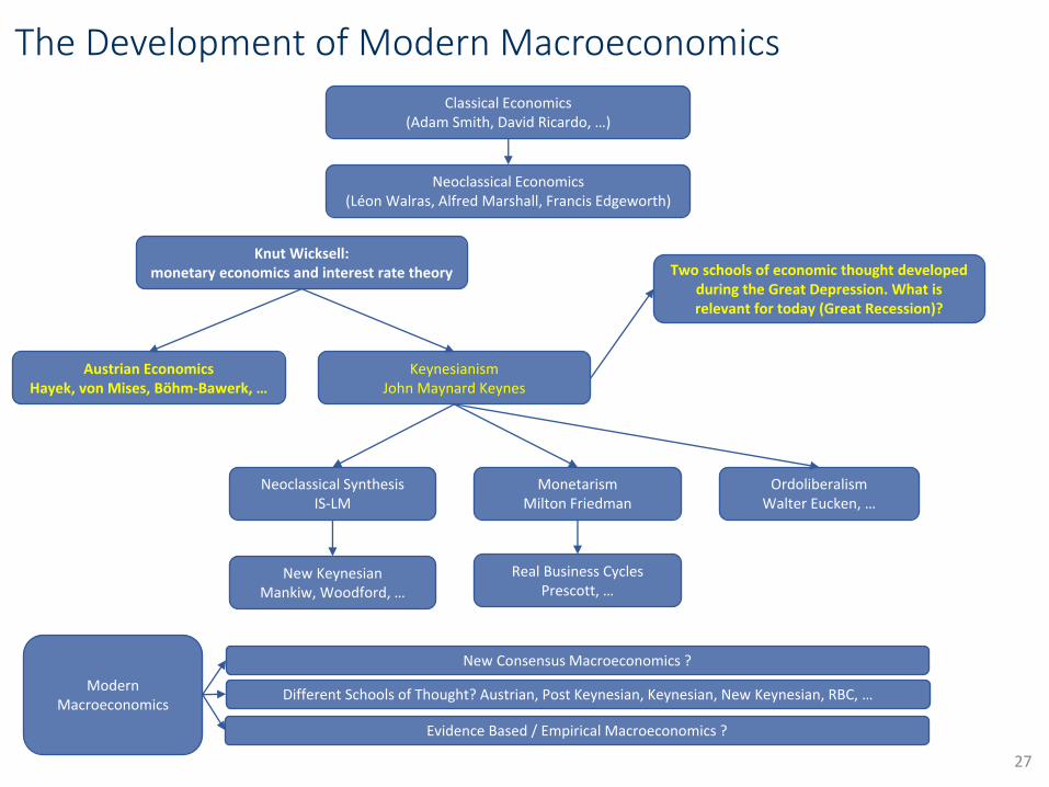
The Development of Modern Macroeconomics

4

Classical Economics (Adam Smith, David Ricardo, …)

Neoclassical Economics (Léon Walras, Alfred Marshall, Francis Edgeworth)

Knut Wicksell: monetary economics and interest rate theory

Austrian EconomicsHayek, von Mises, Böhm-Bawerk, …

KeynesianismJohn Maynard Keynes

MonetarismMilton Friedman

Neoclassical SynthesisIS-LM

New KeynesianMankiw, Woodford, …

Real Business CyclesPrescott, …

OrdoliberalismWalter Eucken, …

New Consensus Macroeconomics ?

Different Schools of Thought? Austrian, Post Keynesian, Keynesian, New Keynesian, RBC, …

Evidence Based / Empirical Macroeconomics ?

Modern Macroeconomics

Crisis of Macroeconomics?

Just before the global financial crisis there seemed to be a consensus on macroeconomics modeling

Blanchard, O. (2009). “The State of Macro”, Annual Review of Economics, Annual Reviews, vol. 1(1): 209-228. “The state of macro is good”.

Woodford, M. (2009). “Convergence in Macroeconomics: Elements of the New Synthesis”, American Journal of Economics – Macro, 1(1): 267-279.

Microeconomic foundations (achieve a similar degree of unity as microeconomics) + New Keynesian theory with rational expectations that integrates supply and demand side views.

Since the crisis: criticism on the state of the profession

Krugman (2016): “The state of macro is bad”. Advertises IS-LM models: “Economists who knew and still took seriously good old-fashioned Hicksian IS-LM type analysis made some strong predictions after the financial crisis”. On DSGE models: “There is a huge amount of sunk intellectual capital in this modeling approach.”

Buiter (2009): “ Most mainstream macroeconomic theoretical innovations since the 1970s (the New Classical rational expectations revolution associated with such names as Robert E. Lucas Jr., Edward Prescott, Thomas Sargent, Robert Barro etc, and the New Keynesian theorizing of Michael Woodford and many others) have turned out to be self-referential, inward-looking distractions at best.”

Ray Fair (2012): Modern macro not sensible or its method not feasible to estimate realistic models. Go back to Cowles-Commission style models.

Since the crisis: reemergence of different schools of thought. Example: disputes on fiscal stimulus and austerity.

5

The Role of Crises for Different Schools of Economic Thought

Macroeconomics, unlike microeconomics, periodically fragments.

No new phenomenon. Macroeconomics was often all about schools of thought. Example, textbook title: „A Modern Guide to Macroeconomics: An Introduction toCompeting Schools of Thought“ (Snowdown et al., 1994).

Even during period of new consensus in macroeconomics, heterodox economistscontinued to organise in schools: neo-Marxists, post-Keynesians, Austrians, …

Schools of thougth are associated with macroeconomic crises, and macro synthesisfollows periods of calm (Wren-Lewis, 2012):

Great Depression Keynesian theory

Stagflation of the 70s Rational expectation revolution (RBC, New Keynesian), Monetarism

Great Moderation New neoclassical synthesis

Great Recession ???

Crises are macroeconomic events schools of thougth important for macroeconomics, not microeconomics

Schools of thought are important in policy debates and public debates aboutgovernment interventions and in some parts of the profession. Overall, lot‘s ofdiversity in academia, ideology not very important.

6

The impact of Wicksell‘s interest rate theoryon modern monetary policy

7


8















Impact on today‘smonetary policy

discussions

The Beginning of Modern Macroeconomics: Wicksell

Knut Wicksell (1851-1926)

Swedish Economist

Work on real and nominal interest rates and their role for the determination of the price level / inflation

Developed the concept of the natural rate of interest rate that is a major element of modern macroeconomic models

The natural interest rate is at the core of current policy debates on low interest rates

Main book: Interest and prices (1898). Same title of Woodford’s monograph from 2003 is no coincidence

Influenced economists from Irving Fisher to John Maynard Keynes to James Buchanan

His students (among them Lindahl, Ohlin, …) formed the influential Swedish school of the 1930s. He died before the international acclaim his work obtained in the 1930s through Keynes and the English translation of some of his major books.

9

Wicksell wanted to understand in detail the effects of an increase of money supply on prices and the additional short-run effects on real income.

He started out with the quantity equation that he viewed as theonly consistent theory regarding the effects of monetary policy.

𝑃𝑌 = 𝑀𝑉

𝑃: Prive level

𝑌: Aggregate income

𝑀: Money

𝑉: Velocity of money

Ironically, he ended up with a new explanation regardingbusiness cycle dynamics that were not caused by money supply, but by the discrepancy between saving and investment.

10

Wicksell‘s studies of the determination of the price level

Quantity Theory of Money

Starting point is the Quantity Equation

Definition of money velocity: 𝑉 = (𝑌 × 𝑃)/𝑀

𝑌: real GDP (volume of real transactions per year)

𝑃: price level

𝑀: money in circulation

Quantity Equation (Identity, correct per definition, not a theory)

𝑉 × 𝑀 = 𝑌 × 𝑃

The left hand side shows how much money is in circulation and how manytimes this used in transactions Value of all transactions

The right hand side shows the nominal GDP Value of all transactions

Both sides show the same, just based on different ways to measure nominal GDP

11

Quantity Theory of Money

Quantity Equation: 𝑉 × 𝑀 = 𝑌 × 𝑃

Quantity Theory is based on two assumptions:

𝑀 is controlled by the central bank

𝑉 and 𝑌 do not depend on 𝑀

It follows that in the medium to long run the central bank fully controlsthe price level and inflation:

If the central bank increases money supply by 𝑥 percent, this leads to an increase in the price level of 𝑥 percent (holding 𝑉 and 𝑌 constant as they do not depend on 𝑀).

𝑉𝑀

𝑌= 𝑃

𝜋 = 𝑔𝑚 + 𝑔𝑣 − 𝑔𝑦

Assuming that the velocity of money is rather constant (𝑔𝑣 = 0)

𝜋 = 𝑔𝑚 − 𝑔𝑦

12

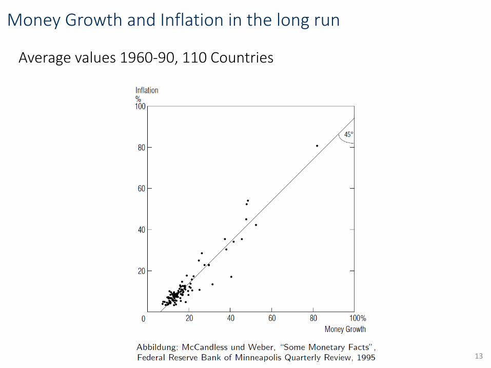
Money Growth and Inflation in the long run

Average values 1960-90, 110 Countries

13

Money supply and price level during hyperinflations

14

(a) Austria (b) Hungary

Money

Price level

Index(Jan. 1921 = 100)

Index(Juli 1921 = 100)

Price level

100.000

10.000

1.000

10019251924192319221921

Money

100.000

10.000

1.000

10019251924192319221921

(c) Germany

1

Index(Jan. 1921 = 100) (d) Poland

100.000.000.000.000

1.000.000

10.000.000.0001.000.000.000.000

100.000.000

10.000100

Money

Price level

19251924192319221921

Price level

Money

Index(Jan. 1921 = 100)

100

10.000.000

100.000

1.000.000

10.000

1.000

19251924192319221921

Investment, Savings and the Credit Market

Classic: no focus on the credit market. Firms financed investment via retainedprofits and savings of workers were low.

Neoclassic: real interest rate leads to market clearing between investmentand savings. Analysis in real terms, money plays no role.

15

S

I

I‘

r

S, I

r

r‘

Investment, Savings and the Credit Market

Wicksell extended the model to include banks and credit creation (in his model there is nocash)

In Wicksell‘s model unlimited credit creation possible, but in reality banks are limited in how much they can lend:

Profitability in a competitive banking system

Prudential regulation acts as a constraint on banks’ activities in order to maintain the resilience of the financial system. Important: capital ratio requirements

Central bank sets the interest rate on central bank reserves and thus influences range of interest rates in the economy, including those on bank loans

Neoclassical model: Savings are necessary for investment.

Wicksell:

Banks create new purchasing power via credit creation that can increases investment.

Increase in investment leads to price increases. The purchasing power of households decrease so thatconsumption decreases (households are foreced to save).

Companies can via getting a credit from the banking sector increase investment via decreasingconsumption (households are forced to save). Investment is independent of savings and depends on credit creation.

16

Assets Liabilities

Δ Granted credit Δ Deposits

Business Cycle Dynamics and Price Effects in Wicksell‘s Model

Impact of Wicksell‘s credit markt analysis:

1. Let to analyses of the role of firms for economic evolution. Innovative firms can via bank credit increase production. This is the central message of Schumpeter‘s “The Theory of Economics Development“ (1934).

2. Analyses of dynamics of demand and supplyWicksell was highly influential forKeynes analyses of business cycle dynamics.

Effects on macroeconomic dynamics and prices:

An increase in economic activity due to credit expansion will lead at some point on capacity constraints on the supply side Prices will increase (via increasing cost forexample for wages).

Changes in relative prices: prices increase with different speed in different sectors, but relative prices will go after a while back to their equilibrium level.

Changes in the overall price level (inflation): parallel increase in all nominal variables. No reason that the price level returns to its previous value.

17

Implications for Monetary Policy

Simple analysis of the Quantity Equation, 𝑃𝑌 = 𝑀𝑉, not sufficient to understandprice developments.

Controlling money, 𝑀, in principle controls 𝑃. But, relevant measure of 𝑀 for theprice level is not the amount of central bank money, but central bank money + money created in the banking sector via credit expansion.

In an expansion investment can increase without leading to an increase in thereal interest rate if credit risk decreases.

Wicksell therefore proposed the stabilization of the economy via settinginterest rates rather than the money supply.

If in an expansion investment increases without leading to an increase in theinterest rate on credit, the centralbank should close this gap by increasing thecentral bank rate and hence make refinancing of banks more expensive.

He defines the natural rate of interest as the interest rate that leads to pricestability.

What matters for price developments, credit expansion and economic activityis the difference between the interest rate in the banking system and thenatural interest rate.

The interest rate by the central bank should be set in a way that the bankinginterest rate equals the natural interest rate implies price stability.

18

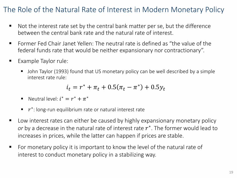
The Role of the Natural Rate of Interest in Modern Monetary Policy

Not the interest rate set by the central bank matter per se, but the differencebetween the central bank rate and the natural rate of interest.

Former Fed Chair Janet Yellen: The neutral rate is defined as “the value of the federal funds rate that would be neither expansionary nor contractionary”.

Example Taylor rule:

John Taylor (1993) found that US monetary policy can be well described by a simple interest rate rule:

𝑖𝑡 = 𝑟∗ + 𝜋𝑡 + 0.5 𝜋𝑡 − 𝜋∗ + 0.5𝑦𝑡

Neutral level: 𝑖∗ = 𝑟∗ + 𝜋∗

𝑟∗: long-run equilibrium rate or natural interest rate

Low interest rates can either be caused by highly expansionary monetary policyor by a decrease in the natural rate of interest rate 𝑟∗. The former would lead toincreases in prices, while the latter can happen if prices are stable.

For monetary policy it is important to know the level of the natural rate ofinterest to conduct monetary policy in a stabilizing way.

19

The gap between the federal funds rate and the naturalinterest rate is what matters

20Source: Rudebusch (2004)

Has the natural interest rate, 𝑟∗, decreased?

The natural interest rate has no explicit value—it is an estimate.

Economists disagree on the range in which the neutral rate falls, and how it might change over time.

Usually, the real neutral interest rate is estimated get the nominal natural interest rate by adding inflation: 𝑖𝑡

∗ = 𝑟𝑡∗ + 𝜋𝑡

Most studies find a decrease in 𝑟𝑡∗ over recent years, but the size

of the decrease is highly disputed.

Reasons for changes in 𝑟𝑡∗:

Demographic changes: people save more for retirement.

Slow-down of potential output growth due to lower labor force and lower technology growth lower investment

Fiscal policy

Changes in the international demand for safe assets (relevant forrecent developments in the US)

21

Natural interest rate estimates of Laubach and Williams

Very low natural rate estimates by Laubach and Williams.

Highly influential on US monetary policy. Yellen referred to these estimates manytimes.

Krugman: “The low natural rate is as solid a result as anything in real time can be”.

22

Implications of different natural interest rates on monetary policy.

Low natural interest rate: set very low interest rates, otherwise danger of deflation:

𝑖𝑡 = 𝑟∗ + 𝜋𝑡 + 0.5 𝜋𝑡 − 𝜋∗ + 0.5𝑦𝑡 ≈ 0 + 𝜋𝑡 + 0.5 𝜋𝑡 − 𝜋∗ + 0.5𝑦𝑡

Yellen (Speech on 19, Jan. 2016): “if the neutral rate were to remain quite low over the medium term, .., then the appropriate setting for R-Star in the Taylor rule would arguably be zero, yielding a yet lower path for the federal funds rate.”

23Source: http://voxeu.org/article/r-star-and-yellen-rules

Has the natural interest rate fallen to 0 %?

24

All recent studies find a decline in the naturalinterest rate, but the size of the decline is very different.

Below point estimates are reported, but uncertainty aroundthese estimates is very high.

Authors 𝒓∗ (recent years) Change since late 90s

Laubach/Williams (2016) 0% -3%

Kiley (2015) 1.25% -0.6%

Lubik/Matthes (2015) 0.5% -2.5%

Pescatori/Turunen (2015) 0.5-1% -2.5%

Johannsen/Mertens (2016) 1.2% -0.5%

Del Negro et al. (2017) 1-1.5% -1 to -1.5%

Wieland/Wolters (2019) 1.2-2.2% -1 to -2%

Conclusion: Wicksell‘s impact on todays monetary policy discussions

Wicksell argued that the quantitaty theory is not sufficient to analyse monetary policy. Money is created endogenously in the banking sector and this is what matters (not the narrow central bank money).

Wicksell defined the concept of a natural interest rate. He found that not the interest rate per se matters for inflation, but the difference between interest rates in the banking sector and the natural interest rate.

This is an important element of how we think nowadays about monetary policy. Over the long run, the central bank cannot control the real rate of interest, i.e. the natural interest rate, that comes from how much people want to save and what opportunities there are for investment. The central bank only controls the short-term banking rate, i.e. the difference to the natural interest rate.

Important to know the natural interest rate to determine the appropriate level of the nominal interest rate, for example via the Taylor rule: 𝑖𝑡 = 𝑟∗ + 𝜋𝑡 + 0.5 𝜋𝑡 − 𝜋∗ + 0.5𝑦𝑡

Wicksell did not study the estimation of the natural interest rate, but thought that monetary policy is appropriate if prices are stable (implying 𝑟𝑡 = 𝑟𝑡

∗).

It turns out that estimating the natural interest rate is difficult and that there is high uncertainty around estimates. The often cited estimates of Laubach and Williams are the lowest in the literature.

Low natural interest rates have large implications for monetary policy: frequency of hitting the zero lowerbound increases.

Even if we get the estimates right and achieve price stability, there is no guarantee of financial stability. Also the model of the credit market by Wicksell has a large influence of how we think about credit creationtoday.

Historical developments very important for current approaches to economic science and economic policy.25

The Great Depression, the Great Recession, Hayek and Austrian Economics

26


27















Two schools of economic thought developedduring the Great Depression. What isrelevant for today (Great Recession)?

The Great Depression

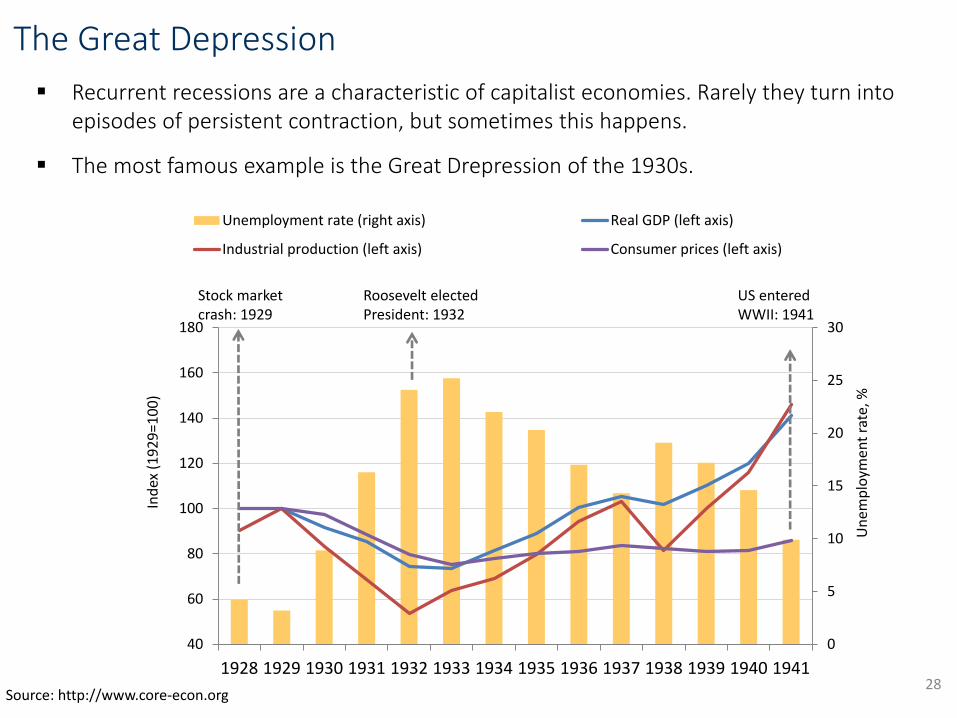
Recurrent recessions are a characteristic of capitalist economies. Rarely they turn into episodes of persistent contraction, but sometimes this happens.

The most famous example is the Great Drepression of the 1930s.

28

0

5

10

15

20

25

30

40

60

80

100

120

140

160

180

1928 1929 1930 1931 1932 1933 1934 1935 1936 1937 1938 1939 1940 1941

Un

emp

loym

en

t ra

te, %

Ind

ex (

19

29

=10

0)

Unemployment rate (right axis) Real GDP (left axis)

Industrial production (left axis) Consumer prices (left axis)

Stock market crash: 1929

Roosevelt elected President: 1932

US entered WWII: 1941

Source: http://www.core-econ.org

Evolution of the Great Depression

Ordinary recession in the late-1920s. Stock market crash of 1929 (cause or symptom?).

Pessimism about the future – households reacted to the 1929 stock market crash by saving more, further decreasing consumption.

Debt and reparations from World War I made the international financial system fragile throughout the 1920s

Main problem: Gold standard (Fixed exchange rate system). Demand of gold increased, but fixed nominal price of gold could not adjust. Hence, all other prices needed to fall Countries needed to deflate their economies to protect the fixed value of their currencies (they also restored to tariffs) deflation debt deflation spiral from ordinary recession to depression.

Banking system failure – many banks failed because loans (partly granted to speculators) could not be repaid; surviving banks raised interest rates. Banking panics in 1930/1931. A series of financial crises occurred from 1931-1933.

Contractionary monetary (Fed raised interest rates in 1928/1929 to stop speculation and in 1931 in response to the international financial crisis). From 1930-1933 money supply fell by 30 % in the US and the Fed did not counteract these developments.

Contractionary fiscal policy.

In the mid-1930s a severe drought occurred.

Great Depression spread from the US to other countries.

29

The Gold Standard as the central cause of the Great Depression

The gold standard fixed the nominal price of gold in terms of its currency.

If the demand for gold were then to increase, the fixed nominal price of gold could not adjust, but all other prices would need to decrease.

As more and more countries rejoined the gold standard, central banks increased their demand for reserves and this increased gold demand.

Problems became severe in the late 1920s when the US and France began attracting large amounts of gold from the rest of the world. A severe deflation of world prices started in mid-1929.

Problems related to deflation:

Real interest rates increased and led to a collapse of investment, debt deflation led to insolvent debtors and a weaker banking system, which led to depositor runs on bank deposits, which in turn further weakened the banking system, and so forth.

Central banks did not easy monetary policy due to the gold standard. Politicians and central bankers clung to the “gold standard mentality,” which viewed the gold parity as an inviolable contract that had to be defended even at the cost of high unemployment (Eichengreen and Temin, 2000). The belief that deflation was a necessary and inevitable adjustment from the preceding boom also provided an excuse to refrain from any significant policy response.

30

Deflation: the good, the bad, the ugly

Good: Productivity/Technology shocks increase output, decrease prices.

Bad: Demand shocks reduce output and prices

Ugly: Self-enforcing deflationary spiral. For example: Irving Fisher‘s (1967-1947) debt-deflation spiral.

31

Price level

A

BC

P0

P1

Output / Income

Aggregierte Demand

Aggreate Supply (new)

Ynat

Aggregate Supply

Demand

YgoodYbad

Pe

Yugly

P2

D

Productivity

Deflation: the good, the bad, the ugly

32

Historical deflation episodes (Borio et al., 2015)

33

Explanations for the Great Depression: Hayek

Friedrich August von Hayek (1899-1992):

Austrian Economist

Nobel price in 1974

In the 1920s important work on business cycles

From the 1930s onwards, he highlighted the problems of central economic planning. His conclusion was that knowledge and information held by various actors can only be utilized fully in a decentralized market system with free competition and pricing.

Together with Carl Menger and Ludwig van Mises the most important economist in the Austrian School of Economics

34

Hayek‘s Monetary Overinvestment Theory

Hayek beliefed that bank credit expansion is a potential problem (as Wicksell).

While Wicksell focused on implications for price stability, Hayek focussed on the relation between pricesfor consumption goods and capital good.

If the bank credit rate deviates from the natural interest rate, it distorts the relative price betweenconsumption and investment.

It drives a wedge between ex ante planned saving and credit/investment. Investment is too high.

Austrian capital theory (Böhm-Bawerk) was the basis for Hayek’s work:

Investment is conducted to build up a capital stock that is finally used for the production of consumption goods. More investment means temporarily less consumption, but higher consumption in the future. Correct price signals are important for this process to work.

If the people prefer postponing consumption and increase saving so that the real interest rate decreases signal to invest more.

Hayek’s monetary overinvestment theory explains crises (Great Depression followed the roaring Twenties, Great Recession followed a housing boom)

Credit expansion in a highly elastic banking system rather than increases in planned savings lead to a quick investment boom. Capacity constraints lead to price increases (consumption demand does not fall as there is no increase in savings). Banks stop granting further credit (increases in prices, risk) or increase the interest rate. Investment projects fail. Credits are not paid back Crisis possible.

Expansionary monetary and fiscal policy could further fuel an overinvestment boom. 35

Relevance of Hayek‘s work for today

Hayek‘s work is praised by the school of Austrian Economics, but has otherwise lost influence. Why?

1. The overinvestment theory could not explain the Great Depression. By 1936 all of net capital accumulation over 1924-29 had been erased (Blanchard, Rhee, and Summers, 1990). Yet the years between 1936 and World War II did not see a restoration of normal levels of activity and unemployment the Great Depression was not caused by an overhang of unproductive capital for the Depression outlasted any plausible such overhang.

2. Liquidation policy deepened the Great Depression: The thinking at that time and in particular Hayek‘swork might have prevented expansionary monetary and fiscal policy which deepened the crisis. Many economists at that time thought that the economy needed to go through a period of "liquidation" in order to lay the groundwork for renewed expansion.

3. Because of the failure of Hayek‘s theories to explain the Great Depression and its in this situationmisguided policy implications, Hayek‘s theories had not much influence after WWII. Keynes (a friend ofHayek) called Hayek‘s theory „one of the most frightful muddles I ever read“. Economists after Keynes (Friedman, Samuelson) do not write about pre-Keynesian theories at all, but base their research fully on Keynes.

But, the conclusion that credit-based boom lead to crises is of very high relevance todayand regains attention (for example at the Bank for International Settlement). Not all, but some business cycles are boom-bust-cycles. For these Hayek‘s analysis is very important.

Examples: US housing boom pre-2008, real estate boom in Portugal and Spain before theEuro crisis. 36

Empirical evidence on the effects of large credit expansions

Schularick and Taylor (Credit Booms Gone Bust, 2012) study the behavior of money, credit, and macroeconomic indicators over the years 1870-2008. They find that credit growth is a powerful predictor of financial crises.

Jorda et al. (When Credit Bites Back, 2013) document that financial-crisis recessions are more costly than normal recessions in terms of lost output; and for both types of recession, more credit-intensive

expansions tend to be followed by deeper recessions and slower recoveries.

37

Sign of financial imbalances and crisis risk: credit fuelled booms (watch out for China these days, but also for global developments: debt has increased globally and is higher than in 2008 BIS Quarterly Review December 2017, Geneva Report 2014 “Deleveraging, What Deleveraging?“).

Good and bad credit growth

Credit growth is not per se a bad thing.

Three out of four periods with high credit growth do not result in a financial crises(Schularick et al, 2017)

Good credit growth: persitently high economic growth due to sustainable investment.

Bad credit growth: short boom due to high consumption growth and unsustainableinvestment. Growth often occurs in the real estate sector (housing and house price boom) rather than in industrial production. Increases in house prices lead to a higher value ofcollateral that is used to increase the volume of credit further.

Policy dicussion: stopping bad credit growth via macroprudential regulation orcontractionary monetary policy.

Figure: credit booms in 17 countries withcrisis (red) and without crisis (white).

Bad credit booms after WWII associatedwith deregulation period after 1980.

38

Austrian Economics

Started with the Methodenstreit with the (German) Historical School (Gustav Schmoller, Max Weber, and partily Joseph Schumpeter). The historical school emphasized historical events and culture-specificeconomics and rejected universal validity of economic theorems, while the Austrian school focussed on genereal valid theories and general economic patterns.

Important economists: Carl Menger, Friedrich von Hayek, August Böhm-Bawerk, Ludwig van Mises

Emphasises

Individual decisions, subjective choices, breaks the macro-micro-dichotomy

Human inter-action (market exchange), entrepreneurship

Limited knowledge, prices as universal information carriers

Aprioristic analytic framework

Set of fundamental claims describing economic/social reality

Strictly deductive logic as ultimate proof only (stressed by van Mises), no empirical analysis, mathematical analysis, models

Liberalism as a social philosophy

Individual economic freedom important for political and moral freedom

Little role for the government: laissez-faire

Business cycle theory: Role of credit boom-bust-cycles

Austrian Economics today

Nowadays considered as a heterodox, rather than part of the mainstream approach to economics. Critics argue that Austrian economics lacks scientific rigor and rejects scientific methods and the use of empirical data in modelling economic behavior.

Many theories of the Austrian School are included in mainstream macroeconomics: marginal utility (Menger), opportunitycost (Wieser), time preference (capital theory of Böhm-Bawerk)

39

Conclusion The Great Depression was caused by tight monetary policy leading to a debt-

deflation spiral. The gold standard was the reason for contractionary monetarypolicy.

Hayek developed based on Wicksell‘s work on the credit and savings market theoverinvestment theory.

He viewed that theory as an appropriate explanation of the Great Depression andproposed liquidations as a policy response to the crisis.

Because of this misguided but influential policy recommendation Hayek‘s theoriesquickly lost influence.

Whether some important theories become mainstream depend crucially on thecircumstances of their development. For example Gustav Cassel‘s prediction thatthe gold standard would lead to a depression became unpopular in the mid 1920s when most economies went into a large boom (roaring twenties).

Hayek‘s theories are of high relevance today Housing boom preceding the Great Recession. High credit growth if invested in unsustainable projects (consumptionand housing booms) are often followed by deep recessions.

Recent empirical evidence based on historical macroeconomic time series data.

Economic developments and policy measure can have a large impact on politicaldevelopments. Austerity policy during the Great Depression contributed to the riseof the Nazi party in Germany, the end of Weimar republic and finally to WWII. Populist and extreme right-wing parties often gain votes after financial crises.

40

The Great Depression, the Great Recession, Keynes vs. Hayek

41


42















Two schools of economic thought developedduring the Great Depression. What isrelevant for today (Great Recession)?

Explanations for the Great Depression: Keynes

John Maynard Keynes (1883 –1946), British Economist

His main book - „A General Theory ofEmployment, Interest and Money“ (1936) –was inspired by the high unemployment rate during the Great Depression.

Keynes was so influential that to his work isoften referred as to the Keynesian revolution.

Economic policy during the 1950s and 1960s was highly influenced byKeynes until the stagflation of the 1970s during which his influence rapidlydeclined.

His work has still a high influence of today‘s economic theory and on economic policy.

43

Keynes three main concepts:

1. The economy is demand driven:

Deficient demand generates output levels too low to induce full employment.

Such unemployment levels can persist for a long period. Even falling prices and wages cannot solve the problem if consumption and investment demand are low due to high uncertainty (prices and wages fell 20-30% during the Great Depression without any endogenous output/employment stabilization).

This justified reference to what Keynes called the possibility of unemployment equilibrium.

2. Liquidity preference theory on interest rate determination:

Interest rates are a monetary phenomenon rather than the real (non-monetary) price determined in the capital market by the ‘supply’ of savings and the ‘demand’ for investment.

3. Saving and investment are not brought into equality by variations in the interest rate, but by changes in the level of income.

Via a multiplier, changes in investment produce changes in income which, with a given propensity to save, produced the savings requisite to finance that investment. Investment is a key variable in income (and employment) generation.

Private investment deficient in terms of its ability to generate full employment, could be supplemented by additional government spending (including public investment) to generate the additional income needed for more employment.

Keynes theory questioned the ability of a free market system (price variations) to clear the labor market (through wage changes) and the capital market (through variations in the rate of interest).

These were revolutionary theoretical principles, with equally revolutionary implications for policy because they questioned the ability of the market system to automatically generate the desired employment (output and income) outcomes.

44

The basic model of the General Theory

At the heart of the General Theory lies the principle of effective demand.

Potential output: there is a certain amount of productive capacity which determines the amount of output which can be produced from the given resources with the given state of techniques. Producing output at potential full employment.

The potential output of the given productive capacity will only eventuate if there is sufficient effective demand for that output. The effective demand is determined by the expectations of sales proceeds of the individual entrepreneurs who control the output decisions.

Up to y′′, the point of full capacity utilization, the effect of an increase in demand is on output.

After y′′ output cannot increase any further and additional aggregate demand raises money income only, that is, it raises the price level. 45

D

yy‘ y‘‘

Supply

Demand‘‘

Demand‘

The nature of effective demand:

Aggregate demand consists of consumption and investment: 𝑌 = 𝐶 + 𝐼

Consumption depends on income: 𝐶 = 𝑐0 + 𝑐1𝑌, with 𝑐0: autonomousconsumption; 𝑐1: marginal prospensity to consume.

Investment depends on its expected profitability (marginal efficiency ofinvestment) and the interest rate: 𝐼 = 𝑓(𝐸, 𝑖)

The interest rate is determined by the supply and demand for money(Keyne‘s liquidity preference theory): 𝑖 = 𝑓(𝐿,𝑀)

Keynesian demand system: four equations, four unknowns: 𝑌, 𝐶, 𝐼, 𝑖

Novelty of Keynes‘ analysis:

The level of effective demand which is determined by this system of equations, need not be the level yielding full capacity utilization output or full employment.

However, if there is unemployment at this level of effective demand, the remedy which suggests itself is additions to aggregate demand.

46

The Keynesian Multiplier:

The dependence of the consumption function on income leads to a multiplier effect:

𝑌 = 𝐶 + 𝐼

= 𝑐0 + 𝑐1𝑌 + 𝐼

Solving for 𝑌:

𝑌 1 − 𝑐1 = 𝑐0 + 𝐼

𝑌 =1

1−𝑐1(𝑐0+𝐼)

Δ𝑌 =1

1 − 𝑐1Δ𝐼

Since 𝑐1 < 1, the multiplier is larger than one.

Given a degree of elasticity in the supply curve, an increase in demand (for example public spending) would generate increased employment and via the additional consumption of domestically produced goods brought about by the new employment, would generate bursts of secondary employment. The amount of secondary employment generated depended on the proportion of the additional income spent on domestic consumption.

This is different than the prevailing view at that time: public spending was seen as useless for stimulating economic activity because it would be offset by an equivalent private investment reduction.

47

Critique of Keyne‘s analysis and its role in modern macroeconomcis

Keynes view:

Keynes viewed his analysis as equilibrium analysis in which a high unemployment rate could occur in the long run, i.e. in equilibrium.

The critique’s view:

This view has often been criticized and opponents argued that Keynes has really modelled possibilities for disequilibrium or temporary equilibrium situations in the labor market.

The modern view

The modern view about Keynes’s conclusions about wages and unemployment, interest rates and savings-investment equality, rests on perceptions of frictions operating in market adjustments which hampers the ability of wages and prices to adjust to achieve the predicted outcome of conventional theory by restricting their flexibility.

Nowadays we think that Keynes view and the predominance of demand is important for short-run fluctuations, while the neoclassical theory of investment and savings is relevant for the medium to long run. In the short run frictions prevent an adjustment of prices and wages to achieve the allocation that would prevail under full price and wage flexibility. In the long run the economy is supply driven.

In the short run an increase in public demand can have stimulative effects, while in the medium to long run it increases interest rates and crowds out private demand.

48

Explanations for the Great Depression: Hayek vs Keynes

Hayek:

The overinvestment theory could explain the Great Depression.

Hayek argued in the spring of 1929 that a recession is inevitable, since the ‘easy money’ policy initiated by the US Federal Reserve Board in July 1927 had prolonged the boom for two years after it should have ended. The collapse would be due to overinvestment in securities and real estate, financed by credit creation.

Liquidation of insolvent firms was the logic consequence.

Keynes

He argued in fall 1928 that the danger lay in the tight monetary policy initiated by the Fed in 1928 in an effort to choke off the asset boom.

Keynes argued that speculation in real estate and stocks had masked a more general tendency to underinvestment in relation to corporate savings.

The danger was the opposite to the one diagnosed by Hayek.

‘If too prolonged an attempt is made to check the speculative position by dear money, it may well be that the dear money, by checking new investment, will bring about a general business depression’. (CW,xiii, 4 October 1928).

For Hayek the depression was threatened by ‘investment running ahead of saving’; for Keynes by ‘saving running ahead of investment’.

Austrians: the slump is not the disease which needed cure, but the cure for the previous disease of over-expansion of credit.

Keynesians: the slump is the desease of too little demand, needing to be cured by more investment.

49

The Great Recession of 2008/2009Development of the real estate bubble in the US

Policymakers intended that households with low income who previously could not afford buying a house were enabled to buy their own property.

Worldwide high savings rate caused by demographic change and previous crises Savings Glut

Highly risky investments were undertaken, but prices did not account sufficiently forrisk:

Low interest rate environment Search for Yield

Insufficient risk management

Deregulation of financial markets new products like asset backed securities.

50

Demand for creditfinanced real

estate increases

Real estate pricesincrease

Banks grant moreloans/mortgages

Indebtness increased

51Quelle: Illing (2016)

Deb

tin

per

cen

to

fav

aila

ble

inco

me

S&P/

Cas

e-Sh

iller

Nat

ion

al H

om

e P

rice

Ind

ex

rela

tive

to

aver

age

inco

me,

19

87

= 1

00

S&P/Case-Shiller National Home Price Index relative to average income, 1987 = 100

Overall debt of private households

Debt with real estate as collateral

When the Fed tightened monetarypolicy, many debtors with a lowcredit rating got into financialproblems.

As they could not pay their rates, the value of asset backedsecurities and other debt contractsfell. The decrease in house pricesaccelerated this process.

A chain reaction with the threat ofbank breakdowns and bankrunsstarted.

The government of the USA decided to bail out some banks, but not all.

52

US mortgages in default

Credit card debt

Spillovers to other sectors

Decreasing asset prices + high indebtness

Less demand and supply for credit

Precautionary savings consumption decreased

Savings paradox: saving more can decrease output temporarily

Pessimism/uncertainty: investment decreased.

Unemployment increased, recession in many sectors (not only real estate, construction and car industry).

→ more insolvencies→ more banks in trouble

International spillovers:

Drop in trade. Less demand for imports from other countries, less demand for exportgoods from the US.

High interconnectedness of financial system (global banks) trouble for financialsystems internationally, less credit supply

53

How did a small problem in the US housing market send theglobal economy to the brink of a catastrophe?

There was rapid growth in the globalization of international capital markets, measured by the amount of foreign assets owned by domestic residents. At the same time, the globalization of banking was occurring. Some of theunregulated expansion of lending by global banks ended up financingmortgage loans to so-called subprime borrower.

Falling real estate prices meant that banks with very high leverage, andtherefore with thin cushions of net worth (equity), in the US, France, Germany, the UK and elsewhere quickly became insolvent.

Fear was transmitted around the world and customers cancelled orders. Aggregate demand fell sharply.

Low regulation of the financial sector. Banks were allowed with great scope tochoose their level of leverage. Banks could use their own models to calculatethe riskiness of their assets. They could meet the international regulatorystandards for leverage by understating the riskiness of their assets, and byparking these risky assets in what are called shadow banks, which theyowned but which were outside the scope of banking regulations.

Many economists continued to believe that economic instability was a thingof the past, right up to the onset of the crisis itself.

54

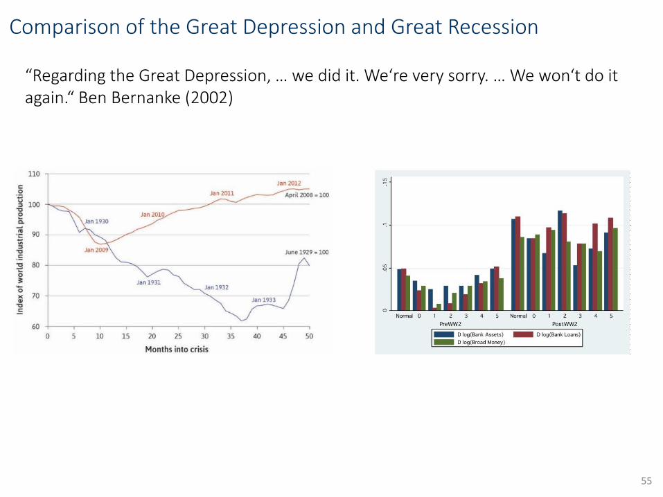
Comparison of the Great Depression and Great Recession

“Regarding the Great Depression, … we did it. We‘re very sorry. … We won‘t do itagain.“ Ben Bernanke (2002)

55

Hayek, Keynes and the Great Recession

Strict Hayekian explanation:

If one believes that the market economy is optimally self-regulating, a large recession can only be due to externally inflicted wounds.

Money glut can then explain the Great Recession. Loose monetary and fiscal policy enabled Americans to live beyond their means. In particular, Alan Greenspan, chairman of the Federal Reserve Board in the critical years leading up to 2005, is said to have kept money too cheap for too long, thus allowing an asset bubble to get pumped up till it burst.

56

Hayek, Keynes and the Great Recession

Strict Keynesian explanation:

Savings glut caused the crisis. Keynesian view that slumps are caused by ‘saving running ahead of investment’.

The origins of the crisis lie in a pile up of saving in East Asia insufficiently offset by new investment in the USA.

Asset inflation which enabled debt-fuelled consumption is common to both stories, but whereas the first sees overinvestment (or malinvestment in Hayekian language) as the culprit, the second puts the blame on excess (Chinese) saving not sufficiently offset by ‘real’ investment.

Mainstream view:

Mispricing of risk (Low financial regulation + loose monetary policy + savings glut)

Overinvestment in real estate recession

Demand crisis in all sectors

Recession accelerated by the zero lower bound on monetary policy

57

From an Hayekian Overinvestment to a Keynesian Demand Crisis

Rognlie, Shleifer, Simsek (2017) explain the Great Recession as a combination of a Hayekian and a Keynesian crises:

Hayek’s overinvestment: excess capital was build during boom years Collapse of the housing price bubble let to two crises:

1. Financial crisis, which led financial institutions that suffered losses related to the housing market to cut back their lending to firms and households (Brunnermeier (2008), Gertler and Kiyotaki (2010)).

2. The reduction in home prices also generated a household deleveraging crisis, in which homeowners that suffered leveraged losses from their housing equity cut back their consumption so as to reduce their outstanding leverage (Guerrieri and Lorenzoni (2011), Eggertsson and Krugman (2012), Mian and Sufi (2014)).

Keynes lack of aggregate demand + zero lower bound: Both crises reduced aggregate demand, plunging the economy into a Keynesian recession. The recession was exacerbated by the zero lower bound on the nominal interest rate.

Problems with a pure Hayekian explanation:

Not clear how low investment in the liquidating sector reduces aggregate output and employment. As noted by Krugman (1998), the economy has a natural adjustment mechanism that facilitates the reallocation of labor (and other productive resources) from the liquidating sector to other sectors. As the interest rate falls during the liquidationphase due to low aggregate demand, other sectors expand and keep employment from falling. This reallocation process can be associated with some increase in frictional unemployment. But it is unclear in the Austrian theory how employment can fall in both the liquidating and the nonliquidating sectors, which seems to be the case for major recessions such as the Great Recession.

To capture that evidence, an additional Keynesian aggregate demand mechanism is needed.

58

Discussion: Bail-out and increase in demand vs. liquidation

During the Great Depression the Fed did not counteract deflationby preventing the collapse of the banking system or by expandingthe monetary base.

During the Great Recession a deflationary spiral was prevented(but what about incentives for future risk taking?)

Liquidation: cold-turkey type recession, reallocation of resources

Bail-outs: sluggish activity, incomplete reallocation of resources

59

Three options of coping with debt crises

Public bail-outs

Shifts private debt to public sector

Private debt crisis sovereign debt crisis

No solution for fiscally distressed countries

Incentive incompatible in general

Inflating the debt away

Takes a long time, promotes zombification

Puts the currency at risk

Not targeted towards non-performing loans

Liquidation

Tough (cold turkey) in the short-run …

… but targeted (and root cause oriented)

Danger of prolonging a recession into a depression

Situation in the Euro Area: no sufficient liquidation

0

50

100

150

200

250

300

350

2000 2002 2004 2006 2008 2010 2012 2014

Protugal Italy Spain Greece Ireland

Gross Private Sector DebtGross Private Sector DebtGross Private Sector DebtGross Private Sector DebtGross Private Sector DebtGross Private Sector DebtGross Private Sector DebtGross Private Sector DebtGross Private Sector DebtGross Private Sector Debt

Annual Data. In relation to nominal GDP.

Gross Private Sector Debt

Percent

12,3

17,3

7,0

34,4

18,9

0

5

10

15

20

25

30

35

40

2000 2002 2004 2006 2008 2010 2012 2014

Portugal Italy Spain Greece Ireland

Annual data. Share of total loans.

Non-Performing Loans

Percent

Non-Performing Loans

Data source: Bank for International Settlements, World Bank.

Monetary financing of governments

0

1

2

3

4

5

6

7

8

2005 06 07 08 09 10 11 12 13 14 15 16

Germany France Italy Spain EMU

Monthly data. EMU: Averrage.

Government Bond Yields (10-year)Government Bond Yields (10-year)Government Bond Yields (10-year)

Percent

Government Bond Yields (10-year)Government Bond Yields (10-year)

0

20

40

60

80

100

120

140

2005 2007 2009 2011 2013 2015

Germany France Italy Spain EMU

Gross Government DebtGross Government DebtGross Government DebtGross Government DebtGross Government DebtGross Government DebtGross Government DebtGross Government Debt

Annual Data. In relation to nominal GDP; EMU: Average.

Gross Government Debt

Percent

Data source: Eurostat, European Commission.

Zombie firms: The Walking Dead

While Hayek‘s explanations for the Great Depression are only popular amongscholars of the Austrian School of Economics probably, they are important for today.

First, the Great Recession of 2008/2009 can partially be explained by Hayek‘s theory.

Second, some of Hayeks‘ policy implications (liquidation) and Schumpeter‘s creativedistruction are also important for today: Zombie firms – defined as old firms that have persistent problems meeting their interest payments –are currently stifling labourproductivity performance in OECD countries. Besides limiting the expansion possibilities of healthy incumbent firms, market congestion generated by zombie firms can also create barriers to entry and constrain the post-entry growth of young firms Prime Example: Italy!

63Source: https://www.oecd.org/eco/The-Walking-Dead-Zombie-Firms-and-Productivity-Performance-in-OECD-Countries.pdf

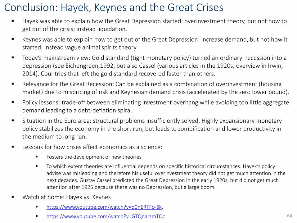
Conclusion: Hayek, Keynes and the Great Crises Hayek was able to explain how the Great Depression started: overinvestment theory, but not how to

get out of the crisis; instead liquidation.

Keynes was able to explain how to get out of the Great Depression: increase demand, but not how itstarted; instead vague animal spirits theory.

Today‘s mainstream view: Gold standard (tight monetary policy) turned an ordinary recession into a depression (see Eichengreen,1992, but also Cassel (various articles in the 1920s, overview in Irwin, 2014). Countries that left the gold standard recovered faster than others.

Relevance for the Great Recession: Can be explained as a combination of overinvestment (housingmarket) due to mispricing of risk and Keynesian demand crisis (accelerated by the zero lower bound).

Policy lessons: trade-off between eliminating investment overhang while avoiding too little aggregatedemand leading to a debt-deflation spiral.

Situation in the Euro area: structural problems insufficiently solved. Highly expansionary monetarypolicy stabilizes the economy in the short run, but leads to zombification and lower productivity in the medium to long run.

Lessons for how crises affect economics as a science:

Fosters the development of new theories

To which extent theories are influential depends on specific historical circumstances. Hayek‘s policyadvise was misleading and therefore his useful overinvestment theory did not get much attention in thenext decades. Gustav Cassel predicted the Great Depression in the early 1920s, but did not get muchattention after 1925 because there was no Depression, but a large boom.

Watch at home: Hayek vs. Keynes

https://www.youtube.com/watch?v=d0nERTFo-Sk,

https://www.youtube.com/watch?v=GTQnarzmTOc 64

https://www.youtube.com/watch?v=d0nERTFo-Sk

https://www.youtube.com/watch?v=GTQnarzmTOc


65















His impact on rule-based monetary policy The impact of Friedman‘s 1967

presidential address.

Milton Friedman

American Economist (1912-2006)

Ph.D. in economics from Columbia in 1946

Full professor of economics at the University of Chicago since 1948

Was awarded the Nobel prize in economics in 1976

Major contributions:

His book “A Monetary History of the United States, 1867-1960” with Anna J. Schwartz published in 1963 is one of the major contributions to Monetarism argued that tight monetary policy was the main cause of the Great Depression; basis for rule based monetary policy, recommend a steady growth of the money stock.

Consumption theory: consumption depends mainly on permanent income, not current income.

Phillips-curve: importance of inflation expectations short-run trade-off between inflation and unemployment, but in the long run vertical Phillips-curve. Concept of the natural rate of unemployment.

Criticized Keynesian stabilization policy: implementation lags and ineffectiveness if not accommodated by monetary policy (crowding out). Advocat of liberalism.

Very active in economic policy advise (Eisenhower, Nixon, Ford, Reagan, Pinochet administration in Chile).

66

Monetarism I

Monetarism is a doctrine which suggests

that money has a major influence on both the level of economic activity and the price level

that the objectives of monetary policy are best realised by targeting the rate of growth of money supply.

As such, monetarism has strong affinities with the quantity theory of money, particularly as exposited by Wicksell and Irving Fisher, but its modern variant is largely associated with the work of Milton Friedman.

Friedman tested the quantity theory of money empirically.

Hi restated it as a theory of the demand for money.

His Monetary History of the United States 1867–1960 (Friedman and Schwartz, 1963) and much subsequent theoretical and empirical work developed arguments on the effects of variations in the quantity of money on national income, prices and output. This included analyses of the relative importance of fiscal and monetary policy (Friedman and Heller 1969)

Other important monetarists are Karl Brunner and Allan Melzer

67

Monetarism II

Criticism of Keynes and advocation of money supply rules

Karl Brunner Brunner coined the name, ‘monetarism’ for the phenomenon for reviving a quantity theory based monetary policy as an answer to Keynesian fiscal policies.

Keynesian public spending policy is ineffective due to a ‘crowding out effect’. Similar to the ‘Treasury view’ against which Keynes had so valiantly fought during the 1930s. If public spending increases without accommodative monetary policy then interest rates increase which leads to reduction private spending.

The supply of money is key for price stability and economic growth.

However, due to variable and long implementation lags it is difficult to predict consequences of monetary changes. Therefore, one cannot use money supply variations as a discretionary tool for economic policy.

Advocation of money supply rules: let money supply grow steadily with the long germ real output growth rate. Seen by monetarist as the best solution for minimizing unwanted fluctuations in economic activity.

Monetarists believe that the competitive market frame work is in any case was far better suited than discretionary monetary or fiscal policy to make the necessary short term adjustments in price and output levels.

68

The Debate over the Conduct of Monetary Policy: Rules vs. Discretion

Monetary Policy Rules:

Monetary policy is set accordingly to a clear rule or formula.

Famous examples:

Monetarists steady money growth rule

The Taylor Rule:

𝑖𝑡 = 𝑟∗ + 𝜋𝑡 + 0.5 𝜋𝑡 − 𝜋∗ + 0.5𝑦𝑡

Helps anchoring inflation expectations, but restricts the possibilities of central banksto respond to extraordinary situations. Increases transparency and accountability.

Discretion:

Central bankers decide on a period by period basis on the appropriate monetarypolicy stance.

More flexibility, but more difficult to gain credibility compared to a rule-basedframework (time inconsistency problem).

In reality no central banks follows a rule mechanically, but it is often referred tomonetary policy rules and the policy stance is often compared to the one impliedby specific monetary policy rules.

69

Rules Versus Discretion: Historical Roots

Economists in favor of rule-based monetary policy

Adam Smith (1776) argued in the Wealth of Nations that “a well-regulated paper-money” could improve economic growth and stability in comparison with a pure commodity standard.

Henry Thornton (1802) wrote in the early 1800s that a central bank should have the responsibility for price level stability and should make the mechanism explicit and “not be a matter of ongoing discretion”

David Ricardo (1824, pp.10-11) wrote in his Plan for the Establishment of a National Bank that government ministers “could not be safely entrusted with the power of issuing paper money” and advanced the idea of a rule guided central bank.

Knut Wicksell (1907) and Irving Fisher (1920) in the early 1900s proposed policy rules for the interest rate or the money supply to avoid the kinds of monetary induced disturbances that led to hyperinflation or depression.

Henry Simons (1936) and Milton Friedman (1948, 1960) continued in that tradition recognizing monetary policy rules—such as a constant growth rate rule for the money supply—would avoid such mistakes in contrast with discretion.

The idea was that a simple monetary rule with little discretion could avoid monetary excesses whether due to government deficits, commodity discoveries, or mistakes by government.

Rules vs. chaotic monetary policy: different from the modern debate on rules vs discretion, where discretionary policy is conducted in a systematic manner.

70

Development of modern monetary policy rules

Keynesian econometric models without expectation formation:

First estimated macroeconomic model by Tinbergen (1936). Keynesian model. Monetarypolicy evaluation: how does the economy react to a one time change in monetary policy.

Over the next decades many such models were developed and used by central banks, e.g. the MPS-model (MIT-PENN-SSRC) was adopted by the Fed in the 1960s.

Starting in the 1970s stochastic dynamic macroeconomic models with clearexpectation formation were constructed.

The conduct of monetary policy was evaluated in terms of the stabilization properties ofpolicy rules rather than one time discretionary policy actions

Models were very large leading to highly complex rules.

The Brookings Model Comparison program in the 1970s and 1980s (see Bryant, Hooper, Mann, 1993) let to the development of simple practical policy rules.

It turned out that rules in which the policy interest rate reacts to real GDP and inflation worked well in these models. Research showed that the interest rate reaction to inflation should be greater than 1, the interest rate reaction to the GDP gap should be greater than 0, and the interest rate reaction to other variables should be small.

Most famous example: The Taylor rule

71

Monetary Policy Rules: The Taylor Rule

Taylor rule: 𝑖𝑡 = 𝑟∗ + 𝜋𝑡 + 𝛼 𝜋𝑡 − 𝜋∗ + 𝛽𝑦𝑡

Neutral level: 𝑖∗ = 𝑟∗ + 𝜋∗

Taylor (1993) found that 𝛼 = 𝛽 = 0.5 and 𝑟∗ = 𝜋∗ = 2% described US monetary policy in the late1980s and early 1990s well

𝑖𝑡 = 2 + 𝜋𝑡 + 0.5 𝜋𝑡 − 2 + 0.5𝑦𝑡

If we oberseve an increase of inflation by 1% then increase the nominal interest rate by more than 1%: 1 + 𝛼

Called the Taylor principle. Ensures that monetary policy is inflation stabilizing. Leads todeterminacy in a wide range of macroeconomic models

Intuition: raise nominal interest rate more than the increase in inflation increase in the real interest rate decrease in economic activity with a lag (sticky prices) decrease of inflation

Optimal policies can be overly fine-tuned to a specific model. That is fine if that model is correct, but not if it is incorrect.

Simple monetary policy rules incorporated basic principles such as leaning against the wind of inflation and output. Because they were not fine-tuned to specific assumptions, they are more robust and work well in a variety of models.

72

Original Taylor rule

73Source: Taylor (1993). “Discretion versus policy rules in practice“, Carnegie-Rochester Conference Series on Public Policy 39: 195-214.

Backside of John Taylor‘s business card

74

Taylor Rule and ECB policy

75Sauer, S. and J.-E. Sturm (2003), Using Taylor rules to understand ECB monetary policy, Munich: CESifo Working Paper, 1110, December.

Success of monetary policy rules

Central banks appeared to be moving toward more transparent rules-based policies in 1980s and 1990s, including through a focus on price stability, and economic performance improved.

This connection between the rules-based policy and performance was detected by Clarida, Gali, and Gertler (2000). There was an especially dramatic improvement compared with the 1970s when policy was highly discretionary.

By the year 2000 many emerging market countries joined the rules based policy approach, usually through inflation targeting. Their improved performance contributed to global stability.

Today: Low and stable inflation world-wide.

But: financial instability (2008/2009). John Taylor argues that this has been caused by deviating from policy rules in the US and worldwide (central banks follow each other)

76

Discretion vs. Rules: Then and Now

1960s: Keynesian school influential in the US:

Paul Samuelson advised John F. Kennedy during the 1960 election campaign and recruited Walter Heller and James Tobin to serve on the Council of Economic Advisers.

Economic Report of the President (1962) made the case for discretion rather than rules. For monetary policy it said that a “discretionary policy is essential, sometimes to reinforce, sometimes to mitigate or overcome, the monetary consequences of short-run fluctuations of economic activity.”

1960s: Friedman argues in favor of rules:

In Capitalism and Freedom (1962)he argued that “the available evidence . . . casts grave doubt on the possibility of producing any fine adjustments in economic activity by fine adjustments in monetary policy—at least in the present state of knowledge . . . There are thus serious limitations to the possibility of a discretionary monetary policy and much danger that such a policy may make matters worse rather than better . . .”

77

Discretion vs. Rules: Then and Now

1960s, 1970s: Keynesian view dominated US monetary policy:

Practitioners put discretionary monetary policies into practice, mainly the go-stop policies that led to both higher inflation and higher unemployment.

Friedman remained a persistent and resolute champion of the alternative view.

1980s, 1990s: systematic rule oriented view dominated US monetary policy:

Friedman’s arguments eventually won the day and US monetary policy under Paul Volcker moved away from an emphasis on discretion in the 1980s and 1990s.

Today:

Economists on one side push for more discretionary monetary policy such as the quantitative easing actions and resist the notion of rules-based monetary policy.

Other economists argue for a return to more predictable and rule-like monetary policy. They argue that the bouts of quantitative easing were not very effective, and that deviations from rules-based policy helped worsen the great recession.

The discussion refers often to Friedman’s original ideas.

78

Friedman‘s 1967 presidential adress

“The Role of Monetary Policy,” published in the March 1968 issue of the American Economic Review.

Agreement that high employment, stable prices and rapid growth are desirable.

Disagreement about the compatibility of these goals.

The role of monetary policy in achieving these goals.

Three sections:

1. What monetary policy cannot do

2. What monetary policy can do

3. How should monetary policy be conducted

79

Historical context and relevance for today

Friedman‘s empirical studies on monetary policy let him conclude that it was contractionary monetary policy that caused the Great Depression, is nowadays themainstream view.

By contrast Keynes thought that the Great Depression occured despite expansionarymonetary policy concluding that monetary policy is not effective and fiscal policybeing the effective alternative.

Friedman shows that most economists during the 1940s thought that monetary policyis ineffective and that fiscal policy should be used to stabilize the economy.

He argues that in the 1960s economists think again that monetary policy is highlyeffective with the primary goal being high employment, while stabilizing inflation isonly the secondary goal.

Friedman is concerned that people expect more from monetary policy than it can do. His speech had a huge impact on modern monetary policy and that we have achievedlow and stable inflation rates globally since the 1980s.

Similar situation today in the Euro area today. Some people seem to believe thatpermanent highly expansionary monetary policy leads to economic stability. We canlearn from Friedman‘s speech that this is not possible and that it is the responsibilityof government to solve structural problems.

80

What monetary policy cannot do (the natural rate hypothesis)

It cannot peg the rate of unemployment for more than very limited periods. Structural factors (minimum wage, social security payments, power of unions, availability of information about job vacancies, hiringand firing costs, …) determine the natural rate of unemployment.

Expansionary monetary policy leads temporarily to more spending andemployment.

After a while prices and wages adjust leading to higher nominal wageswithout changing the real wage that matters for the labor market.

Expansionary monetary policy over a longer time period will lead to an adjustment of inflation expectations and employees demand highernominal wages for the future.

Monetary policy can control nominal variables, not in the long run real variables

81

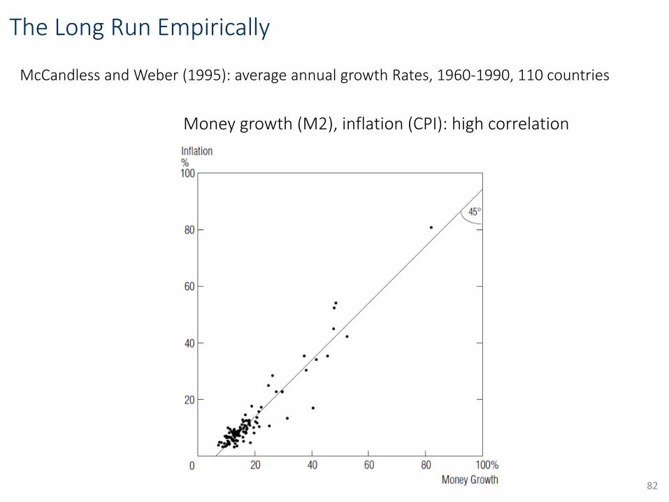
The Long Run Empirically

82

McCandless and Weber (1995): average annual growth Rates, 1960-1990, 110 countries

Money growth (M2), inflation (CPI): high correlation

The Long Run Empirically

83

McCandless and Weber (1995): average annual growth rates, 1960-1990, 110 countries

Money, real output growth: no correlation

Phillips Curve (1960-1969)

Source: Hoover, K. D. (2008). „Phillips Curve”, The Concise Encyclopedia of Economics.84

Expectation augmented Phillips Curve

Short run: Output (unemployment) gap can lead to inflationary pressure

Phillips Curve has a negative slope

Monetary policy can exploit this trade-off in the short-run

Long run: Inflation expectations adjust and equal actual inflation. Inflation is

determined by the money supply

Unemployment equals its natural rate which is determined by real rather than monetary factors

If monetary policy tries to target an unemployment rate below the NAIRU this will lead to inflation rather than unemployment below the NAIRU

85

𝜋𝑡 = 𝜋𝑡𝑒 − 𝛼 𝑢𝑡 − 𝑢𝑛

The Phillips Curve (Short and Long Run)

𝜋𝑡 = 𝜋𝑡𝑒 − 𝛼 𝑢𝑡 − 𝑢𝑛

Expansionary monetary policy leads to a reduction in 𝑢𝑡

Short run: 𝜋𝑡𝑒 = 𝜋𝑡

𝑒, 𝑢1 < 𝑢𝑛 → 𝜋𝑡 ↑

Medium run: 𝜋𝑡𝑒 adjusts → Phillips curve shifts upwards

Long run: 𝜋2𝑒 =𝜋2 → 𝑢2 = 𝑢𝑛 → long-run vertical Phillips curve

86𝑢𝑡

𝜋𝑡

𝑢𝑛

Long-run Phillips curve : 𝑢𝑡 = 𝑢𝑛

A

B

𝜋0

𝜋1

𝑢1

C𝜋2

Short-run Phillips curve (𝜋1𝑒)

Effects of monetary policy

Short run: 𝑢𝑡 < 𝑢𝑛

Long run: 𝑢𝑡 = 𝑢𝑛, 𝜋2 > 𝜋0

Short-run Phillips curve (𝜋2𝑒)

NAIRU: Non-AccelaratingInflation Rate of Unemployment

Source: Hoover, K. D. (2008). „Phillips Curve”, The Concise Encyclopedia of Economics.87

• There is some rate of unemployment that, if maintained, would be compatible with a stable rate of inflation: “nonaccelerating inflation rate of unemployment”

Time variations in NAIRU

Source: Congressional Budget Office88

0,0

2,0

4,0

6,0

8,0

10,0

12,0

19

49

19

51

19

53

19

56

19

58

19

60

19

63

19

65

19

67

19

70

19

72

19

74

19

77

19

79

19

81

19

84

19

86

19

88

19

91

19

93

19

95

19

98

20

00

20

02

20

05

20

07

20

09

20

12

20

14

NAIRU Unemployment rate

There is some rate of unemployment that, if maintained, would be compatible with a stable rate of inflation: “nonaccelerating inflation rate of unemployment”

The Great Inflation

89

What monetary policy can do

1. Avoid being a major source of disturbance: Avoid major mistakes

2. Provide a stable background for the economy: Price stability

3. Contribute to offsetting major disturbances to the economy arising from other sources

“I believe that the potentiality of monetary policy in offsetting other forces

making for instability is far more limited than is commonly believed.

We simply do not know enough to be able to recognize minor disturbances when

they occur or to be able to predict either what their effects will be with any

precision or what monetary policy is required to offset their effects.

In this area [of monetary policy] particularly the best is likely to be the enemy of

the good. Experience suggests that the path of wisdom is to use monetary policy

explicitly to offset other disturbances only when they offer a ‘clear and present

danger’.”

90

How monetary policy should be conducted

Two requirements:

1. Choose target that monetary policy can control:

exchange rate, price level (long and variable transmission lags), broad money (preferred by Friedman)

“Perhaps, as our understanding of monetary phenomena advances, the situation will change. But at the present stage of our understanding the long way around seems the understanding, the long way around seems the surer way to our objective. Accordingly, I believe that a monetary total [aggregate] is the best currently available immediate guide or criterion [target] for monetary policy…”

2. Avoid sharp swings in policy: Achieve steady but moderate rate of growth of specified monetary aggregate

“That is the most that we can ask from monetary policy at our present stage of knowledge. But that much –and it is a great deal –is clearly within our reach.”

91

Modern monetary policy

Monetary targeting

Tried in many countries: Failed and was abandoned

In contrast, inflation targeting has worked fine

Friedman changed his view

Flexible inflation target

Stabilize both inflation around inflation targeting and resource utilization.

Forecast targeting: Choose interest-rate path so forecast of inflation and resource utilization “looks good”.

Why does targeting inflation directly (and stabilizing resource utilization) work?

Better knowledge of transmission mechanism

Role of expectations, transparency, credibility

Good understanding of the Phillips curve

Theoretical developments matched by better empirical methods (Kalmanfiltering, VAR, Bayesian methods)

92

Friedman and modern monetary policy

Friedman’s proposition that monetary policy has no longer-run effect on the real economy was striking.

While in most cases there is first an empirical observation and then theory is developed, e.g. Great Depression Keynesian theory, Friedman predicted that an exploitation of the short-run inflation-unemployment trade-off would only lead to higher inflation, but no reduction in the unemployment rate. The Great Inflation showed that his prediction was correct.

The understanding of the short- und long-run effects of monetary policy, i.e. the short- and long-run Phillips curve, let to low and stable inflation rates globally. Most central banks use inflation targeting.

Current challenges:

Stabilization of inflation and output vs. financial stability

Highly expansionary monetary policy as a source of instability?

Friedman’s presidential address together with the work of Phelps (1967) drew attention to modeling expectation formation. The following rational expectation revolution changed macroeconomicmodels completely.

93

Conclusion I

Debate solved: Keynes vs. Friedman

The mainstream macroeconomic model is the New Keynesian model.

It has emerged from the great economic debates of the past of which wehave examined the views of Keynes and Friedman. We also studied the workof Wicksell, which was important for the work of Keynes and Friedman.

The model is Keynesian in the short run and neoclassical in the long run. The short and long run are connected by changes in expectations inspired byFriedman‘s natural rate hypothesis. Natural rates play an important role asdeveloped by Wicksell. Modern monetary policy is conducted in terms ofinterest rates rather than money (Wicksell vs. Friedman).

Expectations play a key role in modern macroeconomic models (rational expectation revolution started with the Lucas critique).

What monetary policy can do and cannot do is quite clear today (few wouldsuggest that monetary policy should have targets for labor force participation, inequality, the long-term interest rate, …). Credibility, transparency, andmonetary policy rules that anchor expectations are important. Low and stableinflation has been achieved globally.

Important lessons learned: No second Great Depression. 94

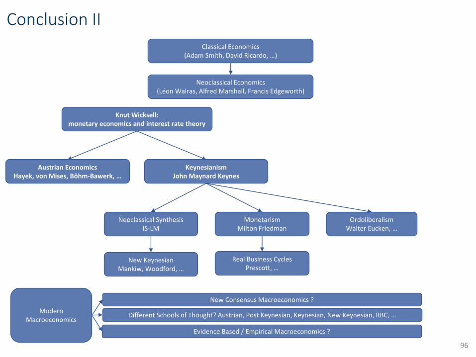
Conclusion II

Ongoing debate: Hayek vs. Keynes

Self regulation of markets vs. stabilizing policies

Both important:

Short-run prevention of crises

Long-run prevention of zombification

Ideological focus mostly in politics, less in academia. For the latter thedifferent views are about focussing on short- vs. long-run developments. But of course not easy to combine appropriate short- and long-run policies.

Modern macroeconomics

Including missing elements, but continuing with dynamic stochastic generalequilibrium models.

Evidence-based empirical work very important (establishing causality)

But danger to loose sight of the long run.

Rules are important to solve time inconsistency problems and political incentivesto focus on the short run.

Work with micro data (firm level, household level, etc.) important as well asworking with historical macro data (very long time series).

95

Conclusion II

96















Conclusion III

Schools of thought still important?

Yes, to understand historical developments and modern macroeconomic models.

Yes, elements from the past are again relevant today. Examples: Hayek‘soverinvestment theory for the Great Recession, Keynes demand theory for the liquiditytrap, Friedman‘s focus on the importance of stable money growth during large recessions.

No, for coming up with appropriate economic policy suggestions. Ideology plays littlerole in academia (yes, for understanding when famous economists are misinterpreted).

Current important questions / challenges:

Expectation formation: what will replace the rational expectation paradigm?

Modeling heterogeneity, nonlinearities

Conducting monetary policy in a low interest rate environment (monetary-fiscalinteraction, financial stability)

Global high debt ratios

Policy in currency unions

Great structural changes: demographics, technology growth / digitalization, inequality

97

Macroeconomics in the Master of Economics program

Goals:

Theory:

Understanding and knowing the most important modern theories

Focus on monetary economics and economic policy (monetary and fiscal) at theChair for Macroeconomics, but there are also lectures on growth, developement, ….

Methods:

Learning empirical methods (macroeconometrics)

Learning deriving and simulating macroeconomic models

Courses

Advanced Macroeconomics

Monetary and Fiscal Policy

Empirical Macroeconomics

Computational Economics

Seminar

98

New major “Quantitative Macroeconomics“ will beintroduced soon.

Documents

Approaches to Economic Science Development of Modern ... fileApproaches to Economic Science Development of Modern Macroeconomics and Different Approaches to Economic Policy Prof. Dr