Applying Multi-Objective Variable-Fidelity Optimization Techniques to

Industrial Scale Rotors: Blade Designs for CleanSky

Gunther WilkeGerman Aerospace Center (DLR) Braunschweig, Institute of Aerodynamics and Flow Technology

Lilienthalplatz 7, 38108 Braunschweig, Germany, gunther.wilke@dlr.de

Abstract

A novel variable-�delity multi-objective optimization technique is applied to the design prob-

lem of helicopter rotorblades of the Green RotorCraft research programme of CleanSky. The

optimization technique utilizes information from aerodynamic low-�delity tools, here a prescribed

wake model in forward �ight and inviscid CFD simulations in hover, to speed-up the high-�delity

optimization, which is based on RANS simulations including all �ve-rotor blades. In reference

to a state-of-the-art single-�delity optimization, this approach �nds about 325% more viable

data points. A choice of three rotorblades from the �nal Pareto frontier of the optimization

is investigated in detail including the o�-design performance as well as acoustic footprint in

an over�ight condition. The �nal outcome is that there does not exist one blade that fully

satis�es all criteria at once, but feasible trade-o�s are found when applying the variable-�delity

multi-optimization technique.

1 INTRODUCTION

The Cleansky JTI (Joint Technology Initiative) is theumbrella project in which the GRC (Green RotorCraft)programme is embedded. The goal of Cleansky is the im-provement of the environmental friendliness of aircraft.This means for GRC to reduce the overall CO2 emmis-sion, as well as the noise impact measured in EPNLand complying with the current and future safety reg-ulations. In GRC 1, innovative rotorblades are investi-gated using active and passive technologies to improvethe blade performance itself and to meet the aforemen-tioned goals. DLR contributed in both categories; on theone hand Riemenschneider et al. [1] test an active bladetwist mechanism on a rotor blade, while on the otherhand Imiela and Wilke [2] focus on the aerodynamic op-timization of blade planform and twist of the rotorblade.This paper re�ects the continued e�ort of the planformoptimization by applying novel methodologies developedby Wilke [3] to obtain even better blades.

In the �eld of numerical rotor optimization in aero-dynamics, many di�erent approaches exist. The com-plexity of the rotor aero-mechanics calls for non-trivialsimulations strategies. The �ow �eld of the rotor is dom-inated by vortices spiced up with transonic and stalledregions, which, when everything is to be modelled cor-rectly, calls for expensive high-�delity CFD simulations.Additionally taking into account the unsteady natureand aero-elastic e�ects of the rotor, the computationale�ort is tremendous. On top of this, numerical optimiza-tion requires many evaluations and thus designing a rotorblade with the help of automized frameworks becomes aweary undertaking.

Therefore many research activities exist to cut downthe computational costs. Dumont et al. [4] demonstratethat by applying the adjoint methodology to a gradi-ent based optimization of a hovering rotor that the costcompared to evaluate the gradients directly with CFD issigni�cantly reduced. Massaro and D'Andrea [5] take adi�erent route and develop a simulation method based

on potential theory with additional measures to take intoaccount viscous e�ects to circumvent the need of CFDsimulations in the optimization. This enables them toperform multi-point optimizations with a genetic opti-mization algorithm. Visingardi et al. [6] also perform anintensive optimization applying simpli�ed aerodynamicmodels to have good turn-around times and computeobjectives in ten di�erent �ight conditions. Other re-searches such as Johnson [7] and Imiela [8] employ surro-gate based approaches to optimize rotor blades in hoverand forward �ight conditions. The surrogate based opti-mization aids the search for the optimum by generating amathematical abstraction from the original simulation,which is then evaluated a lot faster than the originalcomputed code.

Collins [9] was the �rst to join both strategies to-gether; the use of surrogate models with high-�delityCFD and low-�delity models. This methodology is alsoreferred to as multi- or variable-�delity approach. First,a low-�delity surrogate model is generated, where manysimulations can be executed at low cost thus obtain-ing a highly accurate surrogate model (at low-�delitylevel). Then, this model is re-calibrated with a few high-�delity samples to arrive at the global high-�delity op-timum faster than only creating the high-�delity surro-gate purely from high-�delity samples. Wilke [10] per-forms studies on which aerodynamic models are mostsuited for this type of optimization and further re�nedhis variable-�delity framework for multi-objective prob-lems [3]. Latter work also underlined the need for theapplication of multi-objective strategies for the optimiza-tion of rotorblades, as single-objective optimized blades,either for hover or forward �ight, tend to have draw-backs in the other �ight condition. Leon et al. [11]introduces the Nash game approach to rotor blade opti-mization, which is further re�ned in [12], also speedingup their optimization with multi-�delity methods. TheNash game may be (very) brie�y summarized as a gra-dient based method, which starts at the best con�gura-tion of one objective and then gradually moves along the

Pareto front towards the other objective. Another multi-objective technique taking advantage of multiple �deli-ties is applied by Leusink et al. [13]. They start a geneticoptimization at low-�delity level, where they shrink thedesign space after an initial optimization. The obtainedlow-�delity population from the second optimization isthen resampled with the high-�delity to create a high-�delity surrogate model, in which the optimization iscontinued. They, however, do not update their high-�delity surrogate model with novel designs, simply toavoid extensive use of computational resources.

The multi-objective approach proposed by [3], whichwas applied to a model rotor problem with few parame-ters at mid-�delity level, is now applied to the referencerotor blade of the GRC 1 project. Here, the numberof design parameters is increased from four to ten andadditionally the pitch link loads are constrained in both�ight conditions to arrive at more feasible blade plan-forms. The �nal results are already at high-�delity level,thus no re-computation is necessary. A subset of thePareto optimal con�gurations is abstracted and investi-gated in o�-design conditions to further stress the needfor multi-objective optimizations. Besides purely consid-ering the aerodynamic performance, the rotors are alsoanalyzed in a high-speed impulsive noise over�ight con-dition required for certi�cation.

2 METHODOLOGY

In Figure 1, a sketch of the overall optimization pro-cess is given. First, the baseline geometry is parameter-ized with ten design variables. The optimization is thenstarted with a low-�delity design of experiments. Thedesign of experiments samples randomly di�erent rotorgeometries to then generate the �rst initial low-�delitysurrogate models (ylfm) of the returned goal functionsand constraint values, here the required power in hoverand forward �ight along with their maximum pitch linkloads. Within this surrogate model a multi-objectivesearch is performed which generates a new choice of sam-ples to be evaluated with the low-�delity. Upon iterat-ing the process a �nal low-�delity surrogate model isobtained, from which the high-�delity design of experi-ments is generated. To include a greater variety, randomsamples are additionally included to avoid a too strongbias with the low-�delity optima in case these are notmatching with the high-�delity optima. With the �rsthigh-�delity samples evaluated, the variable-�delity sur-rogates are build (yvfm) which are then re�ned with agoal function re�nement of each �ight condition. Theseare basically two individual single-objective optimiza-tions, which are simply coupled by also ful�lling the con-straints of the opposing �ight condition. This is done to�nd the anchor points of the Pareto front, before theactual high-�delity multi-objective search is started tohave a well-conditioned initial performance landscape.Upon completion of this process, the Pareto front of thehigh-�delity sampled con�gurations is generated.

For the reference, the same process is repeated with-out using the low-�delity at all, thus starting from a

completely random design of experiments. The goal isto compare the performance of the single- to the vari-able �delity approach. In the context of multi-objectiveoptimization, the performance cannot be put into hardnumbers, but is compared by the density and distribu-tion of the �nal samples of each approach to judge theperformance.

In the following, the individual parts of the optimiza-tion procedure are described; the design of experiments,the type of surrogate models, the optimization strategywithin the surrogate model and the aerodynamic modelsapplied.

2.1 Design of Experiments

The design of experiments plays an important role insetting up a surrogate based optimization. It can be re-lated to a computational mesh in CFD. A bad mesh willnot allow for good results, even if the solution schemeis of high-order. The same is true for the design ofexperiments; a bad initial surrogate model from an ill-conditioned design of experiments cannot be recoveredby a highly accurate surrogate model. Romero et al. [14]study di�erent types of design of experiments and basedon this study, it is decided to use the central voronoitesselation (CVT), see Ju et al. [15], for purely randomdesign of experiments.

From the investigations in [3] it was seen that whencreating high-�delity design of experiments, it is bene�-cial to simply quick start the optimization with the opti-mum of the previous �delity. However, this design spaceconsists only of four parameters, which contains less lo-cal minima than the ten dimensional space. Therefore,a blend of low-�delity optima, one from hover and fromforward �ight, is sampled along with a CVT cube. Thesingle-high-�delity is purely sampled with a CVT cube.The actual sample numbers for each �delity and processcan be found in Figure 2. Figure 2 also lists the numbersfor the multi-objective update cycles as well as the thegoal function re�nement cycle, which are kept the samefor single- and variable-�delity.

2.2 Surrogate Models

The here employed surrogate models are based onKriging. Kriging models a Gaussian process. On an ab-stract level, Kriging is a combination of a trend functionand an error correction term:

(1) y(~x) = ftrend(~x) + �(~x)

with y(~x) the surrogate function, ftrend(~x) is the trendfunction and �(~x) the error correction term. The mostwidely form of Kriging is universal Kriging, where thetrend function is modelled by a polynomial. Exemplaryfor a one dimensional, second order surrogate this is writ-ten as:

(2) ftrend(x) = �2x2 + �1x

1 + �0x0

Low-FidelityDesign of Experiments

Low-FidelityMulti-Objective Updates

High-FidelityDesign of Experiments

High-FidelityGoal function refinement

High-FidelityMulti-Objective Updates

Forward flight5 bladed

RANS

HoverPeriodic

RANS

Forward flightBET + presc.wake model

HoverPeriodic

EuleryLFM

yVFM

yLFM

yLFM

yVFM

ParetoFront

BaselineRotor

yHV

yFF

Figure 1: Propsed multi-objective variable-�delity optimization process for helicopter rotorblades. Left: the opti-mization process, right: blade geometries and simulation methodologies.

with �2; �1 and �0 the coe�cients to be determined. Ina more general, vectorial form it is written as:

(3) ftrend(x) = ~� � ~f

where ~� contains the coe�cients and ~f the regressionvector. The error term is (usually) made of radial ba-sis functions. These correct the o�set between sampledpoints and the trend function:

(4) �(~x) = ~ (~x)�1(Xs)(~Ys � F(Xs) � ~�)

with ~ the correlation vector between new sample points~x and the given points Xs, the correlation matrix ofthe sample points and F the regression matrix, which ismade of all regression vectors generated by the samplesXs. From the derivation of Kriging, the determinationof the coe�cients ~� is done by a generalized least squaresmethod:

(5) ~� = (FT�1F)�1FT

�1~Ys

For more detailed information on Kriging, the reader isreferred to the book by Forester et al. [16]While universal Kriging is a single-�delity model, it is

easily enhanced to a variable-�delity model. The pro-posed Hierarchical Kriging by Han and Görtz [17] isbased on the idea to exchange the trend function by alow-�delity surrogate model, which may be based on uni-versal Kriging or another Hierarchical Kriging for staged�delity levels. The low-�delity trend function is imple-mented in a slightly modi�ed way in contrast to Han andGörtz and reads:

(6) ftrend(~x) = �ylfm(~x) +

dX

k

(�kxk)

Where the low-�delity model ylfm is scaled by the pa-

rameter � and a multi-linear functionPd

k(�kxk) is addedon top to give more �exibility to the model. The coe�-cients � and � are determined just as in Eq. (5) for thepolynomial trend. The parameter � is also a measure

Hig

h F

idel

ity

Des

ign

of

Exp

erim

ents

Hig

h F

idel

ity

Up

dat

e C

ycle

10 in

divi

dual

s x

10 u

pdat

e cy

cles

300

rand

om s

ampl

esy LFM

y VFM

y LFM

Bo

th L

F O

pti

ma

with

30

ran

dom

sam

ples

Lo

w F

idel

ity

Des

ign

of

Exp

erim

ents

20 in

divi

dual

s x

5 up

date

cyc

les

Lo

w F

idel

ity

Up

dat

e C

ycle

4 in

divi

dual

sX

10 r

efin

emen

t cy

cles

Hig

h F

idel

ity

Go

al f

un

ctio

n r

efin

emen

t

y VFM

10 in

divi

dual

s x

10 u

pdat

e cy

cles

y SFM

50 r

ando

m s

ampl

es4

indi

vidu

als

X10

ref

inem

ent

cycl

es

y SFM

Sin

gle

Fid

elit

y C

ases

(SF

)

Var

iab

le F

idel

ity

Cas

e

(VF

)

Figure 2: Ressource allocation for variable- (VF) andsingle- (SF) �delity optimizations.

initial populationCentral Voronoi Tessellated Hypercube

drive members towards Pareto frontDifferential Evolutionary

optimize each individual towards each goal function

Simplex

y2

y1

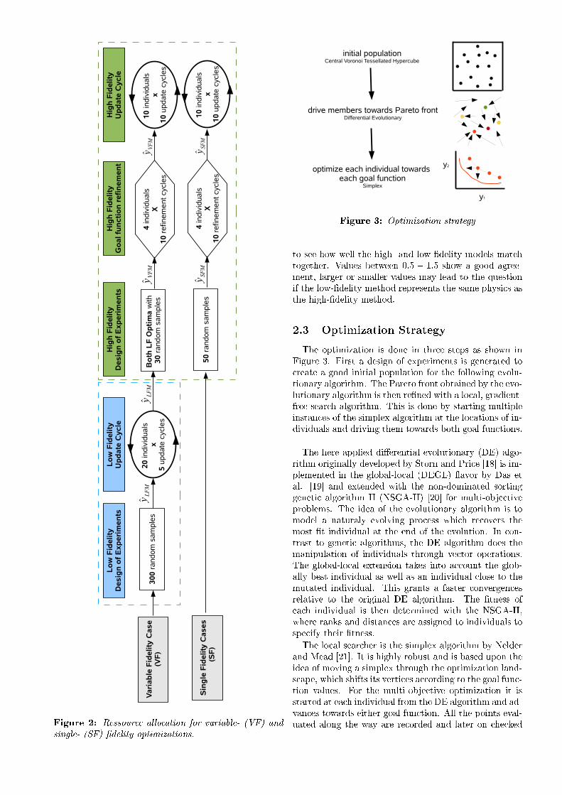
Figure 3: Optimization strategy

to see how well the high- and low-�delity models matchtogether. Values between 0:5 � 1:5 show a good agree-ment, larger or smaller values may lead to the questionif the low-�delity method represents the same physics asthe high-�delity method.

2.3 Optimization Strategy

The optimization is done in three steps as shown inFigure 3. First a design of experiments is generated tocreate a good initial population for the following evolu-tionary algorithm. The Pareto front obtained by the evo-lutionary algorithm is then re�ned with a local, gradient-free search algorithm. This is done by starting multipleinstances of the simplex algorithm at the locations of in-dividuals and driving them towards both goal functions.

The here applied di�erential evolutionary (DE) algo-rithm originally developed by Storn and Price [18] is im-plemented in the global-local (DEGL) �avor by Das etal. [19] and extended with the non-dominated sortinggenetic algorithm II (NSGA-II) [20] for multi-objectiveproblems. The idea of the evolutionary algorithm is tomodel a naturaly evolving process which recovers themost �t individual at the end of the evolution. In con-trast to genetic algorithms, the DE algorithm does themanipulation of individuals through vector operations.The global-local extension takes into account the glob-ally best individual as well as an individual close to themutated individual. This grants a faster convergencesrelative to the original DE algorithm. The �tness ofeach individual is then determined with the NSGA-II,where ranks and distances are assigned to individuals tospecify their �tness.

The local searcher is the simplex algorithm by Nelderand Mead [21]. It is highly robust and is based upon theidea of moving a simplex through the optimization land-scape, which shifts its vertices according to the goal func-tion values. For the multi-objective optimization it isstarted at each individual from the DE algorithm and ad-vances towards either goal function. All the points eval-uated along the way are recorded and later on checked

for Pareto optimality to yield a more re�ned front thanthe di�erential evolutionary algorithm allowed.This search mechanism is limited to �nally yield a

maximum of 1000 individuals in the end. As sampling allthese with a high-�delity is not considered economically,a reduction is performed �rst. The smallest distance toany existing sample is computed for each new individualand they are sorted in descending order. The top ten arethen chosen for evaluation. This is repeated ten timesto arrive at a re�ned surrogate model. This is di�erentfrom the approach in [3], where the locations with thehighest combined model error are chosen. This approachcircumvents the problem of unintentionally weighing theerror of one goal function more than the other and avoidsabundant sampling in already well sampled areas.The treatment of constraints in the multi-objective

context is achieved by checking the constraint value in itsrespective surrogate model and whether the constraint isviolated or not. If it is violated, the individual is consid-ered un�t and receives very large goal function values,thus e�ectively eliminating it from the population or di-verting the simplex algorithm. An implicit and maybetrivial constraint is enforced; the functionality of the ro-tor. If the aero-mechanic code returns that the con�g-uration cannot �y due to the lack of lift or aero-elasticdivergence, the constraint is considered violated, other-wise the rotor passes. This binary result of violated (1.1)or non-violated (0.0) is recorded in an additional surro-gate model referred to as 'crashmap'. If this surrogatemodel returns a value larger than 1, the considered (sur-rogated) individual is considered un�t. The advantage ofthis error treatment is that no penalization or taintingof the goal function surrogate is necessary as no valueneeds to be inserted into it. The point is simply avoidedby its existence in the crashmap.

2.4 Simulation Framework

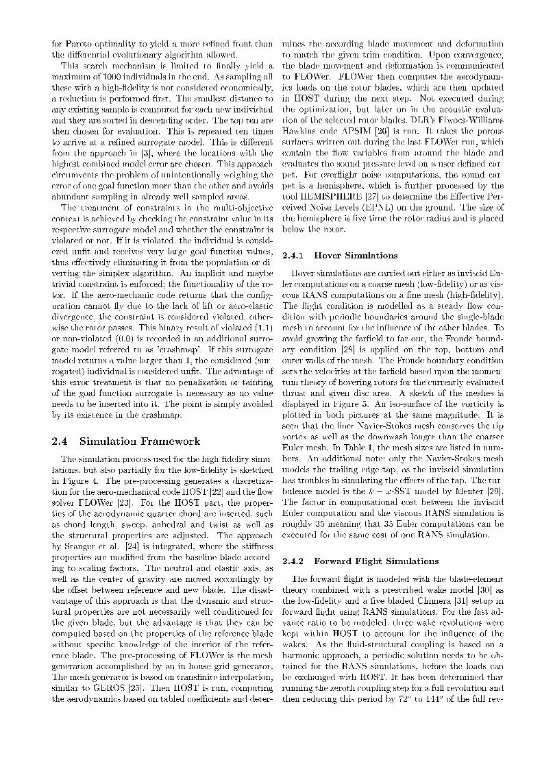
The simulation process used for the high-�delity simu-lations, but also partially for the low-�delity is sketchedin Figure 4. The pre-processing generates a discretiza-tion for the aero-mechanical code HOST [22] and the �owsolver FLOWer [23]. For the HOST part, the proper-ties of the aerodynamic quarter chord are inserted, suchas chord length, sweep, anhedral and twist as well asthe structural properties are adjusted. The approachby Stanger et al. [24] is integrated, where the sti�nessproperties are modi�ed from the baseline blade accord-ing to scaling factors. The neutral and elastic axis, aswell as the center of gravity are moved accordingly bythe o�set between reference and new blade. The disad-vantage of this approach is that the dynamic and struc-tural properties are not necessarily well conditioned forthe given blade, but the advantage is that they can becomputed based on the properties of the reference bladewithout speci�c knowledge of the interior of the refer-ence blade. The pre-processing of FLOWer is the meshgeneration accomplished by an in-house grid generator.The mesh generator is based on trans�nite interpolation,similar to GEROS [25]. Then HOST is run, computingthe aerodynamics based on tabled coe�cients and deter-

mines the according blade movement and deformationto match the given trim condition. Upon convergence,the blade movement and deformation is communicatedto FLOWer. FLOWer then computes the aerodynam-ics loads on the rotor blades, which are then updatedin HOST during the next step. Not executed duringthe optimization, but later on in the acoustic evalua-tion of the selected rotor blades, DLR's Ffwocs-WilliamsHawkins code APSIM [26] is run. It takes the poroussurfaces written out during the last FLOWer run, whichcontain the �ow variables from around the blade andevaluates the sound pressure level on a user de�ned car-pet. For over�ight noise computations, the sound car-pet is a hemisphere, which is further processed by thetool HEMISPHERE [27] to determine the E�ective Per-ceived Noise Levels (EPNL) on the ground. The size ofthe hemisphere is �ve time the rotor radius and is placedbelow the rotor.

2.4.1 Hover Simulations

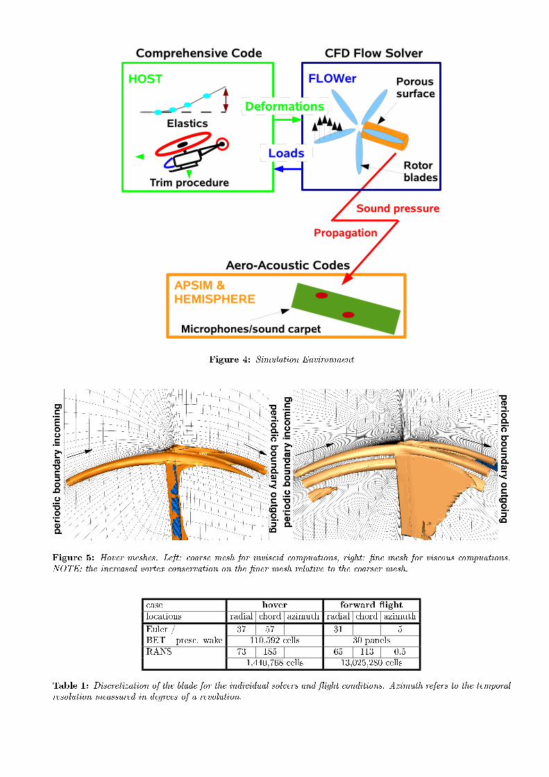
Hover simulations are carried out either as inviscid Eu-ler computations on a coarse mesh (low-�delity) or as vis-cous RANS computations on a �ne mesh (high-�delity).The �ight condition is modelled as a steady �ow con-dition with periodic boundaries around the single-blademesh to account for the in�uence of the other blades. Toavoid growing the far�eld to far out, the Froude bound-ary condition [28] is applied on the top, bottom andouter walls of the mesh. The Froude boundary conditionsets the velocities at the far�eld based upon the momen-tum theory of hovering rotors for the currently evaluatedthrust and given disc area. A sketch of the meshes isdisplayed in Figure 5. An iso-surface of the vorticity isplotted in both pictures at the same magnitude. It isseen that the �ner Navier-Stokes mesh conserves the tipvortex as well as the downwash longer than the coarserEuler mesh. In Table 1, the mesh sizes are listed in num-bers. An additional note; only the Navier-Stokes meshmodels the trailing edge tap, as the inviscid simulationhas troubles in simulating the e�ects of the tap. The tur-bulence model is the k � !-SST model by Menter [29].The factor in computational cost between the inviscidEuler computation and the viscous RANS simulation isroughly 35 meaning that 35 Euler computations can beexecuted for the same cost of one RANS simulation.

2.4.2 Forward Flight Simulations

The forward �ight is modeled with the blade-elementtheory combined with a prescribed wake model [30] asthe low-�delity and a �ve bladed Chimera [31] setup inforward �ight using RANS simulations. For the fast ad-vance ratio to be modeled, three wake revolutions werekept within HOST to account for the in�uence of thewakes. As the �uid-structural coupling is based on aharmonic approach, a periodic solution needs to be ob-tained for the RANS simulations, before the loads canbe exchanged with HOST. It has been determined thatrunning the zeroth coupling step for a full revolution andthen reducing this period by 72o to 144o of the full rev-

Microphones/sound carpet

APSIM & HEMISPHERE

Porous surface

Rotorblades

FLOWer

Sound pressure

Propagation

HOST

Elastics

Loads

Deformations

Trim procedure

Comprehensive Code CFD Flow Solver

Aero-Acoustic Codes

Figure 4: Simulation Environment

Figure 5: Hover meshes. Left: coarse mesh for inviscid compuations, right: �ne mesh for viscous compuations.NOTE: the increased vortex conservation on the �ner mesh relative to the coarser mesh.

case hover forward �ight

locations radial chord azimuth radial chord azimuth

Euler / 37 57 31 5BET+ presc. wake 110,592 cells 30 panelsRANS 73 185 65 113 0.5

1,440,768 cells 13,025,280 cells

Table 1: Discretization of the blade for the individual solvers and �ight conditions. Azimuth refers to the temporalresolution meassured in degrees of a revolution.

olution granted a good compromise between accuracyand cost. The trim procedure ends either after 7 cou-pling steps or if the required power of the rotor changesless than 10�3 relatively. This results in an average of5 coupling steps among the performed simulations. Thediscretization numbers of the forward �ight simulationscan also be taken from Table 1. The cost ratio of thehigh- to low-�delity is 187,000 (!).

3 APPLICATION OF VFM

BASED OPTIMIZATION

3.1 Reference Blade and Parameters

The described variable-�delity optimization method-ology is applied to the GRC reference rotor. The refer-ence rotor depicted in Figure 7 is similar to the modelrotor 7AD blade [32]. The blade features a linear twistdistribution and a parabolic blade tip just as the 7AD,but does not employ any anhedral. The rotor itself has�ve blades with a tip radius of 5.5 m. The two �ightconditions investigated are hover and forward �ight. Inhover, the thrust coe�cient is cT =� = 0:09 and in for-ward �ight cT =� = 0:07. The advance ratio in forward�ight is � = 0:33, the tip Mach speeds are Mtip = 0:65and Mtip = 0:6 in hover and forward �ight respectively.The thrust is trimmed in hover, while in forward �ighta set fuselage drag and required lift are trimmed alongwith the rolling moment.The torque distribution in forward �ight of the base-

line blade is plotted in Figure 8, while the lift- and torquedistribution in hover are plotted in Figure 9. In forward�ight, this blade draws most of its power at the outerradial stations on the retreating blade side and in therear part. Here, the airfoils operate at high angles-of-attack (AoA) to keep the helicopter in balance. A smallsharp red line is identi�ed on the advancing side, whichis attributed to transonic e�ects. In hover, the lift growslinearly to about 80% r/R and then shows a curved peakat about 95%. This behavior comes from the tip vortexof the previous blade, which hits the blade at about 90%r/R. On the one side it increase the lift, on the other itdecreases it. The wiggles in the torque distribution arealso reasoned with the e�ect of tip vortices, yet the ef-fect of the self-induced vortex is noted by the additionalwiggle towards the tip. This comes from the parabolicblade tip, where the self-induced vortex starts when theleading-edge retreats. The acoustic footprint of the bladeonto the hemisphere is drawn in Figure 10. Most soundis generated on the advancing side at the blade tip, whichis coming from the mild shocks on the blade. Anotherregion is identi�ed on the retreating side, which is relatedto the higher loading of the blade tip in this area.The rotor blade is parameterized with non-rational

uniform B-splines (NURBS) [33]. Five twist parametersare chosen along with two sweeping and two taperingparameters and an an-/dihedral parameter. The greatnumber of twist parameters is chosen as the blade twistis the most bene�cial and simplest to accommodate pa-rameter, while the an-/dihedral creates the greatest dif-

0.3 0.4 0.5 0.6 0.7 0.8 0.9 1.0 1.1

r/R

twis

t

anhedra

l, c

hord

, sw

eep

anhedralchordsweeptwistfree control points

Figure 6: Parameterization of GRC blade

�culties from a structural point of view. A picture of theplacement of the parameters is given in Figure 6, whereall NURBS control points are line markers, yet the onesfree to modify by the optimizer are circled in magentawith arrows showing their degree of freedom.

3.2 Optimization Results

The results after running the single- and variable-�delity optimizations are displayed in Figure 11. On theleft, the Pareto fronts obtained by either the single- (4)or variable-�delity (�) are depicted by the red and greenline and markers, respectively. When combining bothset of points together, the theoretical combined Paretofront (�) is colored in magenta. The single-�delity proce-dure found a total of 15 points and the variable-�delity17 points. However, the variable-�delity is mostly moreadvanced than the single-�delity. Therefore, if the con-tributions of both methods is compared to the combinedfront, only 4 points are from the single-�delity and 13from the variable-�delity, thus the variable-�delity re-trieved 325 % more interesting points than the single-�delity. Comparing the costs of both approaches, thesingle-�delity evaluated slightly more high-�delity pointsand thus has a total cost of 82.2 cpu years, while thevariable-�delity including the cost of evaluating the low-�delity (0.15 cpu years) requires 74.4 cpu years. A cpuyear is de�ned as the time it would take a single processor(XEON E5-2695 v2) to perform the presented optimiza-tions. The overall gain of the variable-�delity becomesevident.

3.3 Novel Blades for GRC

For the GRC 1 project, a subset of rotors obtainedfrom these optimizations is chosen to be further studied.Three blades have been picked, namely the anchor pointsof each �ight condition as well as an intermediate design.The blade performing best in forward �ight, referred toas best forward �ight blade is depicted in Figure 12,the best hover blade in Figure 20 and the intermediatechoice, a trade-o� blade, in Figure 16. Their respective

Figure 7: Baseline blade Figure 8: Torque distribution of the baseline blade inforward �ight.

0.3 0.4 0.5 0.6 0.7 0.8 0.9 1.0

r/R 0e+00

1e-04

2e-04

3e-04

4e-04

5e-04

lift (czM2 )

torque (cqM3 )

-6e-07

-4e-07

-2e-07

0e+00

2e-07

4e-07

6e-07

czM2 cqM

3

Figure 9: Torque and lift di�erence distribution of thebaseline blade in hover.

Figure 10: Acoustic footprint on hemisphere of the ref-erence blade.

0.94 0.96 0.98 1.00 1.02 1.04Forward Flight Performance

0.95

1.00

1.05

1.10

1.15

1.20

1.25

1.30

Hover

Perf

orm

ance

SFVFBoth

Figure 11: Comparison of single-(SF) and variable-(VF) �delity Pareto fronts and parameters obtained fromhigh-�delity multi-objective optimizations.

performances in reference to the baseline blade are listedin Table 2. Their o�-design performance is plotted inFigure 25 for hover and in Figure 26 as well in Figure 27for forward �ight.

3.3.1 Best forward �ight blade

The best forward �ight blade has little non-linearblade twist with an early tapered blade tip and sweepsthe blade backward. A mild dihedral is found.In forward �ight, Figure 13, the small blade tip along

with the decrease in the twist gradient beyond 90% r/Rreduces the power requirements in the outer sections. Atthe inboard section of the blade a positive twist gradientis observed, which arises from alleviating the root vor-tex, which is seen at roughly 90o azimuth at the inboardlocation. This is questionable as neither the hub nor theblade attachments are modeled and the strength and lo-cation of the root vortex are likely to be di�erent on thecomplete con�guration.Moving onto the performance in hover, this is strongly

degraded in contrast to the reference blade. In Figure 14it is seen that the lift is strongly decreased beyond 90%r/R. The reason for this is that the �ow separates in

Blade forward �ight hover over�ightreq. power constraint req. power constraint HSI-noise

Best Forward Flight -5.9% -12.4% +30.7% -23.8% -3.3 dBTrade-O� -2.4% -30.5% -2.0% -4.2% -1.1 dBBest Hover +7.9% -12.9% -6.5% -0.5% +9.5 dB

Table 2: Improvements of selected multi-objective rotors. HSI = High-Speed Impuslive

Figure 12: Best forward �ight blade Figure 13: Torque di�erence distribution of the best for-ward �ight blade in forward �ight.

0.3 0.4 0.5 0.6 0.7 0.8 0.9 1.0

r/R

-2e-04

-1e-04

0e+00

1e-04

2e-04

lift difference (∆czM2 )

torque difference (∆cqM3 ) -4e-07

-2e-07

0e+00

2e-07

4e-07

∆czM2 ∆cqM

3

Figure 14: Torque and lift di�erence distribution of thebest forward �ight blade in hover. Values above zero meanan increase in contrast to the reference blade.

Figure 15: Change of the acoustic footprint on hemi-sphere in contrast to the reference blade.

Red means that the optimized performs worse than the reference blade, blue an improvement

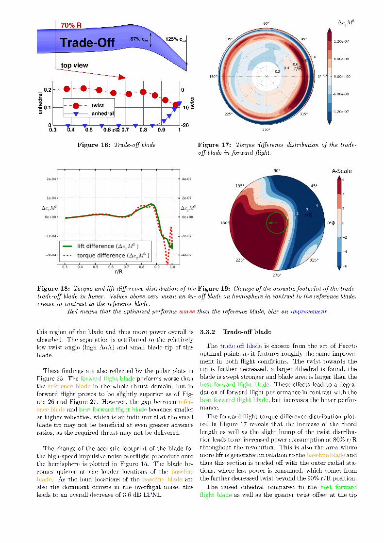
Figure 16: Trade-o� blade Figure 17: Torque di�erence distribution of the trade-o� blade in forward �ight.

0.3 0.4 0.5 0.6 0.7 0.8 0.9 1.0

r/R

-2e-04

-1e-04

0e+00

1e-04

2e-04

lift difference (∆czM2 )

torque difference (∆cqM3 ) -4e-07

-2e-07

0e+00

2e-07

4e-07

∆czM2 ∆cqM

3

Figure 18: Torque and lift di�erence distribution of thetrade-o� blade in hover. Values above zero mean an in-crease in contrast to the reference blade.

Figure 19: Change of the acoustic footprint of the trade-o� blade on hemisphere in contrast to the reference blade.

Red means that the optimized performs worse than the reference blade, blue an improvement

this region of the blade and thus more power overall isabsorbed. The separation is attributed to the relativelylow twist angle (high AoA) and small blade tip of thisblade.

These �ndings are also re�ected by the polar plots inFigure 25. The forward �ight blade performs worse thanthe reference blade in the whole thrust domain, but inforward �ight proves to be slightly superior as of Fig-ure 26 and Figure 27. However, the gap between refer-ence blade and best forward �ight blade becomes smallerat higher velocities, which is an indicator that the smallblade tip may not be bene�cial at even greater advanceratios, as the required thrust may not be delivered.

The change of the acoustic footprint of the blade forthe high-speed impulsive noise over�ight procedure ontothe hemisphere is plotted in Figure 15. The blade be-comes quieter at the louder locations of the baselineblade. As the loud locations of the baseline blade arealso the dominant drivers in the over�ight noise, thisleads to an overall decrease of 3.6 dB EPNL.

3.3.2 Trade-o� blade

The trade-o� blade is chosen from the set of Paretooptimal points as it features roughly the same improve-ment in both �ight conditions. The twist towards thetip is further decreased, a larger dihedral is found, theblade is swept stronger and blade area is larger than thebest forward �ight blade. These e�ects lead to a degra-dation of forward �ight performance in contrast with thebest forward �ight blade, but increases the hover perfor-mance.

The forward �ight torque di�erence distribution plot-ted in Figure 17 reveals that the increase of the chordlength as well as the slight bump of the twist distribu-tion leads to an increased power consumption at 80% r/Rthroughout the revolution. This is also the area wheremore lift is generated in relation to the baseline blade andthus this section is traded o� with the outer radial sta-tions, where less power is consumed, which comes fromthe further decreased twist beyond the 90% r/R position.

The raised dihedral compared to the best forward�ight blade as well as the greater twist o�set at the tip

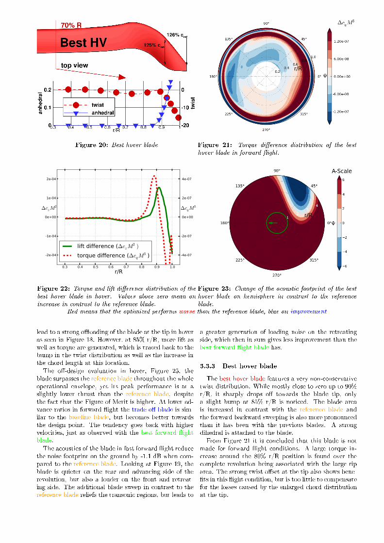
Figure 20: Best hover blade Figure 21: Torque di�erence distribution of the besthover blade in forward �ight.

0.3 0.4 0.5 0.6 0.7 0.8 0.9 1.0

r/R

-2e-04

-1e-04

0e+00

1e-04

2e-04

lift difference (∆czM2 )

torque difference (∆cqM3 ) -4e-07

-2e-07

0e+00

2e-07

4e-07

∆czM2 ∆cqM

3

Figure 22: Torque and lift di�erence distribution of thebest hover blade in hover. Values above zero mean anincrease in contrast to the reference blade.

Figure 23: Change of the acoustic footprint of the besthover blade on hemisphere in contrast to the referenceblade.

Red means that the optimized performs worse than the reference blade, blue an improvement

lead to a strong o�oading of the blade at the tip in hoveras seen in Figure 18. However, at 85% r/R, more lift aswell as torque are generated, which is traced back to thebump in the twist distribution as well as the increase inthe chord length at this location.

The o�-design evaluation in hover, Figure 25, theblade surpasses the reference blade throughout the wholeoperational envelope, yet its peak performance is at aslightly lower thrust than the reference blade, despitethe fact that the Figure of Merit is higher. At lower ad-vance ratios in forward �ight the trade-o� blade is sim-ilar to the baseline blade, but becomes better towardsthe design point. The tendency goes back with highervelocities, just as observed with the best forward �ightblade.

The acoustics of the blade in fast forward �ight reducethe noise footprint on the ground by -1.1 dB when com-pared to the reference blade. Looking at Figure 19, theblade is quieter on the rear and advancing side of therevolution, but also a louder on the front and retreat-ing side. The additional blade sweep in contrast to thereference blade reliefs the transonic regions, but leads to

a greater generation of loading noise on the retreatingside, which then in sum gives less improvement than thebest forward �ight blade has.

3.3.3 Best hover blade

The best hover blade features a very non-conservativetwist distribution. While mostly close to zero up to 90%r/R, it sharply drops o� towards the blade tip, onlya slight bump at 85% r/R is noticed. The blade areais increased in contrast with the reference blade andthe forward-backward sweeping is also more pronouncedthan it has been with the previous blades. A strongdihedral is attached to the blade.

From Figure 21 it is concluded that this blade is notmade for forward �ight conditions. A large torque in-crease around the 80% r/R position is found over thecomplete revolution being associated with the large tiparea. The strong twist o�set at the tip also shows bene-�ts in this �ight condition, but is too little to compensatefor the losses caused by the enlarged chord distributionat the tip.

Figure 24: Cut through the blade with plot of the axialvelocity through the blade. Tip is at 100% R.

From Figure 22 an interesting fact is discovered; theblade recovers energy from the �ow beyond the 90% r/R.The reason for this is that the strong twist o�set alongwith the blade sweep and dihedral cause this portion ofthe blade to be aligned in the upwind region of the previ-ous tip vortex. The resulting force on the airfoils in thatregion is pointed forwards instead of backwards, simi-lar to autorotation or windmill cases. In the downwindsection of the previous tip vortex, the blade area is in-creased and the bump in the twist distribution is found,which compensates for the otherwise lost lift. This costsmore drag, but with the recovery mechanism from theouter blade tip, the sum is less than with the referenceblade. To illustrate the mechanism, Figure 24 picturesthe locations of up and downwash caused by the bladesas well as the previous tip vortex. Beyond 90% r/R astrong upwash is noticed, which allows for the energy re-covery. Note, a perpetu mobile cannot be created withthis mechanism, as the price for the tip vortex has to bepaid �rst, before it can be exploited, which will alwaysbe higher than the actual recovery.

The o�-design performance shows a reciprocal behav-ior to the best forward �ight blade. In hover, Figure 25,the blade surpasses the reference blade over the wholethrust range and has its peak Figure of Merit well pastthe baseline blade, which would also make it suitable forheavy lifting. However, it is not suited for forward �ight,as it draws more power over the complete velocity range,Figure 26. Unlike the other two blades, it decreases itsgap with the reference blade at higher velocities, likelybecause a higher thrust is needed and the enlarged areamight prove bene�cial at greater advance ratios, if otherissues such as aero-elastic divergence do not occur, Fig-ure 27.

Evaluating the acoustic footprint on the ground in thehigh-speed over�ight condition, the blade becomes a lotnoisier than the baseline blade by 9.5 dB EPNL. Thisis related to the large tip area, which causes strongertransonic e�ects and when looking at the hemisphericalsound distribution, it is seen that this makes the bladenoisier in almost all regions, Figure 23

4 CONCLUSIONS

The multi-objective technique developed by Wilke [3]for the variable-�delity optimization of helicopter rotor

0.06 0.07 0.08 0.09 0.10 0.11 0.12

ct/σ

80

85

90

95

100

105

110

FM/FM

ref·1

00%

BaselineBest HVTrade-off

Best FFdesign point

Figure 25: Figure of Merit over thrust blade in hover

blades has been applied within the Green RotorCraft re-search programme of CleanSky to design potential futureblade designs.This multi-objective approach revealed very promising

results. First, it demonstrated that the application ofvariable-�delity approaches leads to a much denser andadvanced Pareto front than applying only one �delitywhen using roughly the same amount of resources. Sec-ondly, it underlined the importance to go with a multi-objective optimization strategy, as otherwise only bladesare found that either optimize the hover or the forward�ight condition, which lead to contrary designs. Thirdly,a set of three potential blade designs is retrieved andstudied in further detail.It is seen that the pure forward �ight or hover blades

actually perform worse in the opposing �ight condi-tion. The multi-objective approach allowed for a goodtrade-o� to accommodate both. However, if helicopterswere designed for single-purposes, or at least their rotorblades, the forward �ight blade might be a promising de-sign for fast VIP transport to remote regions. The hoverblade might also be suited for heavy lifting for a heli-copter of this class or long-endurance surveillance mis-sions. The trade-o� blade however, could be a potentialsuccessor to current blade designs, which are themselvesalready trade-o�s between these two mission types. Thisblade also shows similarities to the ERATO design [34]despite the fact that latter has been optimized for acous-tics.Upon evaluating the sound emission of these blades in

high-speed impulsive �ight conditions, it was found thatblade sweep is not the only answer to reduce the shock onthe advancing side regions. The hover blade features thegreatest blade sweep, however due to its thicker blade atthe tip, it becomes overall louder than the other blades.The slim, yet only mildly swept blade for forward �ightthen proved to be the quietest blade among the onesinvestigated.

0.00 0.05 0.10 0.15 0.20 0.25 0.30 0.35 0.40µ

50

60

70

80

90

100

110

120P(µ

)/Pref(µ

=0.

33)·1

00%

design pointBaselineBest HVTrade-offBest FF

Figure 26: Required power in forward �ight for variousadvance ratios

0.00 0.05 0.10 0.15 0.20 0.25 0.30 0.35 0.40µ

10

5

0

5

10

15

∆P(µ

)/Pref(µ)·1

00%

design pointbaselineBest HVTrade-offBest FF

Figure 27: Relative performance di�erence to referenceblade in forward �ight for various advance ratios

5 AKNOWLEDGEMENTS

The research leading to these results has received fund-ing from the European Community's Seventh FrameworkProgramme (FP7/2007-2013) for the Clean Sky JointTechnology Initiative under grant agreement no CSJU-GAM-GRC-2008-001.

References

[1] J. Riemenschneider, R. Keimer, and S. Kalow: Ex-perimental Bench Testing of an Active-Twist Rotor.In: 39th European Rotorcraft Forum, 2013

[2] M. Imiela and G. Wilke: Passive Blade Optimiza-tion and Evaluation in O�-Design Conditions. In:39th European Rotorcraft Forum, 2013

[3] G. Wilke: Multi-Objective Optimizations in RotorAerodynamics using Variable Fidelity Simulations.In: 39th European Rotorcraft Forum, 2013

[4] A. Dumont, A. Le Pape, J. Peter and S. Huber-son: Aerodynamic Shape Optimization of HoveringRotors Using a Discrete Adjoint of the Reynolds-Averaged Navier-Stokes Equations. In: Journal ofAmerican Helicopter Society 56 (2011), 032002-1-11

[5] A. Massaro and A. D`Andrea: Multi-Point Aero-dynamic Optimization by Means of Memetic Algo-rithm for Design of Advanced Tiltrotor Blades. In:39th European Rotorcraft Forum, 2013

[6] A. Visingardi, L. Federico, and M. Barbarino:Blade Planform Optimization for a Dual Speed Ro-tor Concept. In: 38th European Rotorcraft Forum,2012

[7] C. Johnson: Optimisation of Aspects of RotorBlades using Computational Fluid Dynamics, Uni-versity of Liverpool, Dissertation, 2012

[8] M. Imiela: Mehrpunktoptimierung eines Hub-schrauberrotors im Schwebe- und Vorwärts�ugunter Berücksichtigung der Fluid-Struktur-Wechselwirkung, Institut für Aerodynamik undStrömungstechnik Braunschweig, Dissertation,2012

[9] K. B. Collins: A Multi-Fidelity Framework forPhysics Based Rotor Blade Simulation and Opti-mization, Georgia Institute of Technology, Disser-tation, 2008

[10] G. Wilke: Variable Fidelity Optimization of Re-quired Power of Rotor Blades: Investigation ofAerodynamic Models and their Application. In:38th European Rotorcraft Forum, 2012

[11] E. R. Leon, A. Le Pape, J-A. Desiderie, D. Alfano,M. Costes: Concurrent Aerodynamic Optimizationof Rotor Blades Using a Nash Game Method. In:AHS 69th Annual Forum, 2013

[12] E. R. Leon, J-A. Desiderie, A. Le Pape, and D. Al-fano: Multi-Fidelity Concurrent Aerodynamic Op-timization of Rotor Blades in Hover and ForwardFlight. In: 40th European Rotorcraft Forum, 2014

[13] D. Leusink, D. Alfano, and P. Cinnella: Multi-�delity optimization strategy for the industrial aero-dynamic design of helicopter rotor blades. In:Aerospace Science and Technology 42 (2015), Nr.0, 136 - 147. � ISSN 1270�9638

[14] V. J. Romero, J. V. Burkardt, M. D. Gunzburger,and J. S. Peterson: Comparison of pure and "La-tinized" centroidal Voronoi tessellation against var-ious other statistical sampling methods. In: Reli-ability Engineering & System Safety 91 (2006), S.1266�1280

[15] L. Ju, Q. Du, and M. Gunzburger: Probabilis-tic methods for centroidal Voronoi tessellations andtheir parallel implementations. In: Parallel Com-puting 28 (2002), S. 1477�1500

[16] A. Forrester, A. Sòbester, and A. Keane: Engi-neering Design via Surrogate Modelling - A Practi-cal Guide. John Wiley & Sons Ltd., 2008. http:

//dx.doi.org/10.1002/9780470770801

[17] Z.-H. Han, and S. Görtz: A Hierarchical KrigingModel for Variable-Fidelity Surrogate Modeling. In:AIAA Journal 50-9 (2012), 1885-1896

[18] R. Storn, and K. Price: Di�erential Evolution -A simple and e�cient adaptive scheme for globaloptimization over continuous spaces. In: Journal ofGlobal Optimization 11 (1997), S. 341�359

[19] S. Das, A. Abraham, U. K. Chakraborty, andA. Konar: Di�erential Evolution Using aNeighborhood-Based Mutation Operator. In: IEEETransactions on Evolutionary Computation 13-3(2009), S. 526�

[20] K. Deb, A. Pratap, S. Agarwal, and T. Meyarivan:A fast and elitist multiobjective genetic algorithm:NSGA-II. In: IEEE Transactions on EvolutionaryComputation 6 (2002), apr, Nr. 2, S. 182 �197. �ISSN 1089�778X

[21] J.A. Nelder, and R. Mead: A simplex function forminimization. In: Computer Journal 8-1 (1965), S.308�313

[22] B. Benoit, A.-M. Dequin, K. Kampa, W. von Grün-hagen, P.-M. Basset, and B. Gimonet: HOST, aGeneral Helicopter Simulation Tool for Germanyand France. In: American Helicopter Society 56thAnnual Forum, Virginia Beach, Virginia, May 2-4,2000, 2000

[23] J. Raddatz, and J. Fassbender: Block structuredNavier-Stokes solver FLOWer. MEGAFLOW - Nu-merical Flow Simulation for Aircraft Design. In:Notes on Numerical Fluid Mechanics and Multidis-ciplinary Design 89 (2005), S. 27�44

[24] C. Stanger, M. Hollands, M. Kessler, and E.Krämer: Adaptation of the Dynamic Rotor BladeModelling in CAMRAD for Fluid-Structure Cou-pling within a Blade Design Process. In: 18. DGLR-Fach-Symposium der STAB, 2012

[25] C. B. Allen: CHIMERA volume grid generationwithin the EROS code. In: Proceedings of the In-stitution of Mechanical Engineers, Part G: Journalof Aerospace Engineering 214 (2000), 125-140

[26] J. Yin, and J. Delfs: Improvement of DLR Ro-tor Aeroacoustic Code (APSIM) and its Validationwith Analytic Solution. In: 29th European Rotor-craft Forum,, 2003

[27] J. Yin, and H. Buchholz: Toward Noise AbatementFlight Procedure Design: DLR Rotorcraft NoiseGround Footprints Model. In: Journal of Ameri-can Helicopter Society 52 (2007), April, Nr. 2, S.90�98

[28] P. Beaumier, C. Castellin, and G. Arnaud: Per-formance prediction and �ow�eld analysis of ro-tors in hover, using a coupled Euler/Boundary layermethod. In: 24th European Rotorcraft Forum, 1998

[29] F.R. Menter: Two-Equation Eddy-Viscosity Tur-bulence Models for Engineering Applications. In:AIAA-Journal 32 (1994), S. 1598�1605

[30] G. Arnaud, and P.Beaumier: Validation ofR85/Metar on the Puma RAE Flight Tests. In:18th European Rotorcraft Forum, 1992

[31] T. Schwarz: Ein blockstrukturiertes Verfahren zurSimulation der Umströmung komplexer Kon�gura-tionen, Institut für Aerodynamik und Strömung-stechnik Braunschweig, Dissertation, 2005

[32] M. Allongue and J.P. Drevet: New rotor test rig inthe large Modane wind tunnel. In: 15th EuropeanRotorcraft Forum, 1989

[33] Piegl, Les and Tiller, Wayne: The NURBS Book(2nd Ed.). New York, NY, USA : Springer-VerlagNew York, Inc., 1997. � ISBN 3�540�61545�8

[34] J. Prieur, J. and W. R. Splettstoesser: ERATO - AnONERA-DLR Cooperative Programme On Aeroa-coustic Rotor Optimization. In: 25th European Ro-torcraft Forum, 1999