APPLYING DIFFERENT WIDE-AREA RESPONSE-BASED CONTROLS TO

DIFFERENT CONTINGENCIES IN POWER SYSTEMS

A Thesis

Submitted to the Faculty

of

Purdue University

by

Shahrzad Iranmanesh

In Partial Fulfillment of the

Requirements for the Degree

of

Master of Science in Electrical and Computer Engineering

August 2019

Purdue University

Indianapolis, Indiana

ii

THE PURDUE UNIVERSITY GRADUATE SCHOOL

STATEMENT OF THESIS APPROVAL

Dr. Steven Rovnyak, Chair

Department of Electrical and Computer Engineering

Dr. Brian King

Department of Electrical and Computer Engineering

Dr. Euzeli Cipriano dos Santos

Department of Electrical and Computer Engineering

Approved by:

Dr. Brian King

Head of Graduate Program

iii

To my husband Mehdi,

my parents Monir, and Mohammad Hassan.

iv

ACKNOWLEDGMENTS

First and for the most, I would like to express my sincere gratitude to my advisor

Dr. Steven M. Rovnyak for the continuous support of my Master study and my thesis,

for his patience, motivation, and immense knowledge. His guidance helped me in all

the time of research and writing of this thesis. He shared his knowledge and expertise

with me as well as his time and attention to every detail. He was always available to

answer my questions.

I would also like to thank my advisory committee members Dr. Brian King, and

Dr. Euzeli Cipriano dos Santos for their time and support during the completion of

this thesis.

I would like to specially express my appreciation to Dr. Brian King, who granted

me with brilliant advice and guidance during this degree whenever I needed help.

I would like to extend my special thanks to the Purdue School of Engineering and

Technology, IUPUI, all the faculty and staff who facilitated my thesis work specially

to Sherrie Tucker for her kindness in formatting this thesis and for keeping me in

mind for every important date or opportunity in the ECE Department.

Finally, I must express my gratitude to my husband Mehdi and to my parents for

providing me with unfailing support and continuous encouragement throughout my

years of study and through the process of researching and writing this thesis. This

accomplishment.

v

TABLE OF CONTENTS

Page

LIST OF TABLES . . . . . . . . . . . . . . . . . . . . . . . . . . . . . . . . . . vii

LIST OF FIGURES . . . . . . . . . . . . . . . . . . . . . . . . . . . . . . . . . viii

ABBREVIATIONS . . . . . . . . . . . . . . . . . . . . . . . . . . . . . . . . . . x

ABSTRACT . . . . . . . . . . . . . . . . . . . . . . . . . . . . . . . . . . . . . xi

1 INTRODUCTION . . . . . . . . . . . . . . . . . . . . . . . . . . . . . . . . 1

1.1 Problem Statement . . . . . . . . . . . . . . . . . . . . . . . . . . . . . 1

1.2 Previous Work . . . . . . . . . . . . . . . . . . . . . . . . . . . . . . . 2

1.3 Tools of this thesis . . . . . . . . . . . . . . . . . . . . . . . . . . . . . 6

1.4 About this thesis . . . . . . . . . . . . . . . . . . . . . . . . . . . . . . 8

2 FEATURE EXTRACTION AND INDICES . . . . . . . . . . . . . . . . . . 9

2.1 Bus frequency and bus magnitude . . . . . . . . . . . . . . . . . . . . . 9

2.2 Integral Square Generator angle (ISGA) . . . . . . . . . . . . . . . . . 10

2.3 Calculation of ISBA . . . . . . . . . . . . . . . . . . . . . . . . . . . . 11

3 SENSITIVITY ANALYSIS BASED ON ISBA . . . . . . . . . . . . . . . . . 13

3.1 Overview . . . . . . . . . . . . . . . . . . . . . . . . . . . . . . . . . . . 13

3.2 Result of ISBA Correlations For Two Sample buses . . . . . . . . . . . 13

3.3 Sensitivity analysis of a set of buses . . . . . . . . . . . . . . . . . . . . 14

4 OPTIMIZATION METHOD FOR ONE-SHOT CONTROL . . . . . . . . . 21

4.1 Overview . . . . . . . . . . . . . . . . . . . . . . . . . . . . . . . . . . . 21

4.2 Gradient Descent Method . . . . . . . . . . . . . . . . . . . . . . . . . 21

4.2.1 Gradient Descent Result Without the Presence of an Event . . . 23

4.2.2 Gradient Descent Result With the Presence of Event . . . . . . 26

4.3 Particle Swarm Optimization Method . . . . . . . . . . . . . . . . . . . 27

4.3.1 The Result of PSO Algorithm For a Test Event . . . . . . . . . 28

vi

Page

4.3.2 The Result of the PSO algorithm for a Set of Events . . . . . . 30

5 DECISION TREES FOR CONTROL SELECTION . . . . . . . . . . . . . 33

5.1 Overview . . . . . . . . . . . . . . . . . . . . . . . . . . . . . . . . . . . 33

5.2 Control combinations . . . . . . . . . . . . . . . . . . . . . . . . . . . . 33

5.3 Data sets . . . . . . . . . . . . . . . . . . . . . . . . . . . . . . . . . . 34

5.4 Algorithm . . . . . . . . . . . . . . . . . . . . . . . . . . . . . . . . . . 37

5.5 Implementation of the method . . . . . . . . . . . . . . . . . . . . . . . 39

5.6 Result . . . . . . . . . . . . . . . . . . . . . . . . . . . . . . . . . . . . 41

6 CONCLUSION . . . . . . . . . . . . . . . . . . . . . . . . . . . . . . . . . . 48

REFERENCES . . . . . . . . . . . . . . . . . . . . . . . . . . . . . . . . . . . . 49

A Decision Trees visual representation . . . . . . . . . . . . . . . . . . . . . . . 51

vii

LIST OF TABLES

Table Page

3.1 The variations of RMSBA on ADELANTO and INTERMT buses . . . . . 14

3.2 Selection of buses with maximum variation in RMSBA . . . . . . . . . . . 16

3.3 The variations of RMSBA and NStab for the five selected buses . . . . . . 17

3.4 Comparison of three control combinations for the set of events including480 1-phase events . . . . . . . . . . . . . . . . . . . . . . . . . . . . . . . 19

3.5 Comparison of three selected control combinations for the set of eventsincluding 480 3-phase events . . . . . . . . . . . . . . . . . . . . . . . . . . 20

4.1 Ten selected buses for the optimization algorithms . . . . . . . . . . . . . . 23

4.2 Gradient Descent result without event . . . . . . . . . . . . . . . . . . . . 24

4.3 Gradient Descant result with presence of an event . . . . . . . . . . . . . 26

4.4 The result of PSO algorithm for 7 different cases . . . . . . . . . . . . . . 29

4.5 27 buses where control is applied using the PSO algorithm . . . . . . . . . 30

4.6 PSO results for 8 sample events . . . . . . . . . . . . . . . . . . . . . . . . 31

5.1 The detail of three control combinations . . . . . . . . . . . . . . . . . . . 35

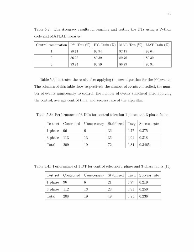
5.2 The Accuracy results for learning and testing the DTs using a Pythoncode and MATLAB libraries. . . . . . . . . . . . . . . . . . . . . . . . . . 44

5.3 Performance of 3 DTs for control selection 1 phase and 3 phase faults. . . . 44

5.4 Performance of 1 DT for control selection 1 phase and 3 phase faults [13]. . 44

viii

LIST OF FIGURES

Figure Page

1.1 Transmission lines for the 176-bus model of WECC [16] . . . . . . . . . . . 7

2.1 Normalized indices for a specific event happened at 0.55 . . . . . . . . . . 12

2.2 Bus voltage magnitudes for a specific event happened at 0.55 . . . . . . . . 12

3.1 Number of stabilized control versus delta RMSBA . . . . . . . . . . . . . . 15

3.2 Number of stabilized events versus delta RMSBA . . . . . . . . . . . . . . 18

4.1 Minimum J/ISGA versus iteration . . . . . . . . . . . . . . . . . . . . . . 24

4.2 Active power versus iteration . . . . . . . . . . . . . . . . . . . . . . . . . 25

4.3 Generator rotor angles before applying control rules of combination 7 . . . 25

4.4 Generator rotor angles after applying control rules of combination 7 . . . . 26

4.5 Minimum J[k] versus k for row 1 of Table 4.3 . . . . . . . . . . . . . . . . 27

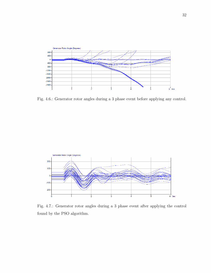
4.6 Generator rotor angles during a 3 phase event before applying any control. 32

4.7 Generator rotor angles during a 3 phase event after applying the controlfound by the PSO algorithm. . . . . . . . . . . . . . . . . . . . . . . . . . 32

5.1 Training data. . . . . . . . . . . . . . . . . . . . . . . . . . . . . . . . . . . 36

5.2 Testing data. . . . . . . . . . . . . . . . . . . . . . . . . . . . . . . . . . . 38

5.3 A sample decision tree. . . . . . . . . . . . . . . . . . . . . . . . . . . . . . 40

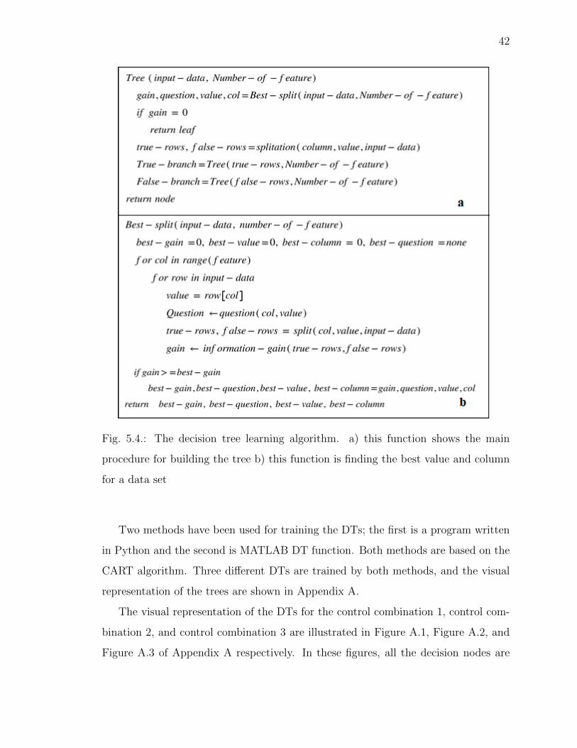
5.4 The decision tree learning algorithm. a) this function shows the mainprocedure for building the tree b) this function is finding the best valueand column for a data set . . . . . . . . . . . . . . . . . . . . . . . . . . . 42

5.5 Generator rotor angles during a 3 phase event before applying the controlselection algorithm. . . . . . . . . . . . . . . . . . . . . . . . . . . . . . . . 45

5.6 Generator rotor angles during a 3 phase event after applying the controlselection algorithm and selecting control combination 2. . . . . . . . . . . . 46

5.7 Generator rotor angles during a 3 phase event before applying the controlselection algorithm. . . . . . . . . . . . . . . . . . . . . . . . . . . . . . . . 46

ix

Figure Page

5.8 Generator rotor angles during a 3 phase event after applying the controlselection algorithm and selecting control combination 3. . . . . . . . . . . . 47

A.1 DT representation of control combination 1 . . . . . . . . . . . . . . . . . 51

A.2 DT representation of control combination 2 . . . . . . . . . . . . . . . . . 52

A.3 DT representation of control combination 3 . . . . . . . . . . . . . . . . . 53

x

ABBREVIATIONS

WECC Western Electricity Coordinate Council

DT Decision Trees

HIF High Impedance Fault

PMU Phasor Measurement Unit

DG Dispersed Generation

WAMS Wide-Area Monitoring Systems

TSAT Transient Security Assessment Tool

PSAT PowerFlow and Short circuit Assessment Tool

SLD Single Line diagram

UFLS Under Frequency Load Shedding

PSO Particle Swarm Optimization

AI Artificial Intelligent

ISGA Integral Square Generator angle

ISBA Integral Square Bus Angles

RMS Root Mean Square

SLG Single Line to Ground

NN Neural Network

xi

ABSTRACT

Iranmanesh, Shahrzad. M.S.E.C.E., Purdue University, August 2019. Applying Dif-ferent Wide-Area Response-Based Controls to Different Contingencies in Power Sys-tems. Major Professor: Steven Michael Rovnyak.

The electrical disturbances in the power system have threaten the stability of the

system. In the first step, it is necessary to detect these electrical disturbances or

events. In the next step, a proper control should apply to the system to decrease the

consequences of the disturbances.

One-shot control is one of the effective methods for stabilizing the events. In this

method, a proper amount of loads are increased or decreased to the electrical system.

Determining the amounts of loads, and the location for shedding is crucial. Moreover,

some control combinations are more effective for some events and less effective for

some others. Therefore, this project is completed in two different sections. First,

finding the effective control combinations, second, finding an algorithm for applying

different control combinations to different contingencies in real time.

To find the effective control combinations, sensitivity analysis is employed to locate

the most effective loads in the system. Then in order to find the control combination

commands, gradient descent and PSO algorithm are used in this project. In the

next step, a pattern recognition method is used to apply the appropriate control

combination for every event. The decision tree is selected as the pattern recognition

method.

The three most effective control combinations found by sensitivity analysis and

PSO method are used in the remainder of this study. A decision tree is trained for each

of the three control combinations, and their outputs are combined into an algorithm

xii

for selecting the best control in real time. Finally, the algorithm is evaluated using a

test set of contingencies. The final results reveal a 30% improvement in comparison

to the previous studies.

1

1. INTRODUCTION

1.1 Problem Statement

Providing reliable and stable electrical power is one of the crucial subjects in the

operation of the electrical systems. Because of the electrical faults in power stations,

damages to electric transmission lines or loss of transmission equipment, the power

supply faces many difficulties. On occasion the intensity of some disturbances are

high enough to cause the generators losing their synchronization, so a black-out may

happen. In some situations, cascading outages may happen in the electrical grid. The

Northeast Blackout of 2003 is an example; when a failure to trim trees in Ohio set

off a chain of events across the grid that ultimately cut power to 55 million people in

eight U.S. states and Canada.

One of the important issues in the electrical system is how to devise techniques for

fault detection, and stabilizing them using proper control method. Therefore, after

fault detection, selecting an effective combination of control actions and applying it

to the system is very important to avoid the spread of faults through the electrical

network.

To resolve this issue, the main aim of previous projects and researches was to

control and stabilize electrical disturbances in the electrical transmission system [1–3].

In order to achieve this goal, several steps should be accomplished. The first step is

event detection, then instability prediction and finally, applying appropriate control

to stabilize the events. Pattern recognition methods have been proposed to process

wide-area phasor measurements and decide when to apply a combination of one shot

controls. However, finding a proper algorithm that categorizes events based on their

characteristics and chooses among different control options are not investigated in the

recent studies, and it worthwhile to put some efforts into answering this question.

2

The main focus of this project is developing a new method to stabilize more events

in an electrical transmission model compare to previous researches. Therefore, there

are two main questions that should be answered in this project. First, what are the

best control options? Second, among all the control combinations, which one is more

effective for a specific event? In fact, we want to find an algorithm that can select

between different control combinations for different contingencies. Accordingly, we

need to use the classification method to classify events based on their characteristics

and apply the appropriate control combinations.

1.2 Previous Work

Numerous studies have been done with the purpose of detecting disturbances and

applying a variety of control methods to stabilize them. Basically, many authors used

pattern recognition methods to address the concerns related to electrical disturbances

in the power systems.

Pattern recognition methods are proposed for many applications in power sys-

tem [4–8].The main contribution of [4] is utilizing High Impedance Fault (HIF) de-

tection method based on DTs as pattern recognition method. In [4], only current

signals are processed, and six features are extracted as inputs to the DT for detecting

HIF. Consequently, the DT algorithm can recognize HIF from normal operation in

the power system. In [5], an Empirical Mode Decomposition (EMD) was performed

to extract Intrinsic Mode Functions (IMF). The Hilbert Transform is applied as a

very effective method for analyzing non-stationary signals. A different pattern recog-

nition approach has been addressed in [6], in which, the authors proposed an island

detection and optimal load-shedding scheme for radial distribution systems combined

with Dispersed Generation (DG). Using a Probabilistic Neural Network-based (PNN)

classifier and exploiting phase-space technique, a passive islanding detection is intro-

duced in [6]. Precisely, they used the Extreme Learning Machine (ELM), which is a

neural network with only one hidden layer that randomly assigns values to weights

3

and biases and calculates the output analytically. The advantage of ELM is fast

training speed. However, since the ELM assigns the initial weight and bias values

randomly, there is a problem of consistency in the results. To prevent the inconsis-

tencies, ensemble models were used, so the results from a number of ELMs were used

to derive the final result. In [7] two neural network methods have been investigated.

Multi-Layer Perceptron (MLP) and Radial Basis Function (RBF) were used for the

classification, and MLP was chosen since RBF needs more than 150 neurons in the

hidden layer for achieving mean square error close to zero. In [7], a total of thirteen

features were extracted such as skewness, kurtosis, form factor, and crest factor to

train an artificial neural network for islanding detection. These features are used to

detect islanding when there is a deviation in Rate of Change of Frequency (ROCOF).

Lidula in [8] employed DT, and Discrete Wavelet Transform (DWT) of the voltage

and current to configure the features.

Pattern recognition method has been proposed in [3, 9] for stability prediction.

Rovnyak and et. al in [3] used DT as a pattern recognition method. The DT predictors

in [3] are R and Rdot, which are apparent resistance and its rate of change measured

near the electrical center of Pacific AC Intertie. They created a DT that could be

used for response based control but control was not tested in the paper. In [9], the

real-time classification was done with Recurrent Neural Networks (RNN), the long-

term dependencies were resolved by Long Short Term Memory (LSTM). The pattern

recognition method in [3, 9], however, does not include any control action.

In some studies, pattern recognition methods are applied to predict islanding in

the power system [10]. Diao [10] used the DTs and synchronized phasor measurement

to detect loss of synchronism and separate the network into pre-defined islands. A

different approach is used for training of the DT in [10]; in fact, one DT is trained

for each contingency instead of training one DT for all of the contingencies. Diao [10]

used the voltage phase angles measurement of high voltage buses, and for each phase

angle variables, they defined six features.

4

Some of the studies proposed islanding control method after instability prediction

to maintain the frequency [11, 12]. The island management method proposed in

[12] can maintain synchronism within each island. The feasible islanding interval is

studied in [11] for applying island control method. The island control method can be

considered as a backup for the control method in the current study.

In some other studies, pattern recognition is used to order control that keeps syn-

chronization and avoids the need for islanding. Gao and et al. [2] used two different

approaches for DT construction process, and one of the methods resulted in a smaller

region of feature space that is stable. The smaller region of space that is stable re-

sults in earlier detection of instability. Gao and et al. [2] used 68 features as predictor

calculated or measured using the Phasor Measurement Unit (PMU). One of the main

contributions of [2] is that they used the one-shot control to avoid the loss of synchro-

nism occurred by the events rather than splitting the electrical grid into islands. The

algorithm in [2] really does order control that keeps synchronization and avoids need

for islanding. Mei and et.al [1] suggested a method to develop response-based decision

trees to activate control for stabilizing the events. The control used in [1,2] is a fixed

combination of power changes in four buses, but in the current study, the algorithm

can select among control options. In [13], the authors used Wide-area Monitoring

Systems (WAMS) to communicate the phase angle data measured by Phasor Mea-

surements Units (PMU). They used pattern recognition methods like DT, to apply

a one-shot control. They employed the combination of separate event detection and

control DTs for transient stability control. Their control actions included disconnec-

tion of costly generation and load. Moreover, to train the DT, they applied some

old and new indices. Eventually, the results show a higher rate of success stabilizing

events using one shot control. The control used in [13] is a fixed combination of power

changes in four buses. A novel Under Frequency Load Shedding (UFLS) algorithm is

used in [14]. In [14] the authors proposed a three stages scheme as a new centralized

5

adaptive load shedding. The first stage includes analyzing the required data and

sizing the reactive power. In the second step, the optimal amount of loads and their

locations are specified. Finally, the third stage includes determining the event type.

A new control strategy is proposed in [15], which can choose between two sets of

control rules. In addition to DTS for event detection and instability prediction, the

author used a third decision tree to apply a proper one-shot control, so the number of

stabilized cases was improved to 30 events. One of the drawbacks with this project is

that they found the control options by trial and error method. In the current project,

on the other hand, numerical methods are used to find a variety of control options.

The main goal of the current thesis project is to stabilize faults or electrical dis-

turbances in the electrical transmission system. To begin, previous works of Rovnyak

and et.al are studied [1–3, 13]. Furthermore, the goal is to increase the number of

stabilized events in comparison to previous studies. In order to achieve this goal, we

developed techniques for controlling events. Moreover, instead of two control options,

three control options are selected in the current study.

The control application area of this project is referred to as one-shot control, which

is a proposed control method to prevent the loss of synchronism and preserving the

security of both transmission and generation during disturbances. The conventional

one-shot control determines the size and the number of the load to change, and

regardless of the location and intensity of the disturbance applies a constant load

scheme. However, in the current project, a new algorithm is developed, that can

apply different control options to different contingencies.

For developing this algorithm, this project is established in three steps. In the

first step, a sensitivity analysis has been developed to locate the most effective buses.

Besides, an optimization technique is exploited for finding the proper amount of loads

to be shed and determining the location of load changes. Particle Swarm Optimiza-

tion (PSO) and Gradient Descent are used as two optimization methods. MATLAB

6

programming is employed for developing the algorithm, and TSAT is used for tran-

sient analysis. The results of optimization algorithms help us to find different control

schemes.

In the last step, a pattern recognition method has been applied to create decision

criteria for deciding to actuate control and select one of several control combinations.

Basically, the pattern recognition methods are Artificial Intelligent (AI) methods.

The study model in this project is the Western Electricity Coordinating Council

(WECC) as represented in Figure 1.1. Different types of 1-phase and 3-phase dis-

turbances are simulated using TSAT, and the data are analyzed using MATLAB.

Various types of features are calculated based on the recorded data. In addition, two

sets of Training and and Test data are are produced to train and test the controlling

algorithm technique.

1.3 Tools of this thesis

Two power system software tools are used in this project. Transient Security

Assessment Tool (TSAT) and PowerFlow and Short circuit Assessment Tool (PSAT).

TSAT is a software tool, established by Powertech Labs Inc., for transient anal-

ysis of power systems. Using the benefits of Transient Security Assessment (TSA),

this software has features for online and off-line TSA analysis. It is a nonlinear

time-domain simulation engine, which has the ability to produce precise responses

to various types of contingencies happening in large interconnected power systems.

It has various applications such as time-domain simulation for processing large and

complex power system models and determination of system stability [17].

On the other hand, PSAT is another software tool by Powertech Labs Inc. It is

a graphical program for building and adjusting power flow data by drawing Single

Line diagram (SLD) and solving power flow. The solution of power flow analysis is

7

Fig. 1.1.: Transmission lines for the 176-bus model of WECC [16]

represented both in tables and on diagrams. In addition to the modification of power

flow models, it has applications in harmonic analysis, short-circuits, and contingency

assessment [18].

8

1.4 About this thesis

In the next chapter, applied features and related equations are evaluated. In the

third chapter, sensitivity analysis is used to locate the most effective buses. In the

fourth chapter, the optimization method and the related results are described. In the

fifth chapter, the detail of the AI method, which is DT is explained, and the final

results related to this project are assessed.

9

2. FEATURE EXTRACTION AND INDICES

A variety of Indices or predictors can be used for Sensitivity analysis and pattern

recognition method in this project. Some of the studies used only two predictors since

using a two-dimensional feature space that can be visualized like R-Rdot application

in [1] is easier to study. In another study [2], voltage angle, voltage magnitude and

their rate of change are exploited as the predictors. In this project, a large number

of predictors are calculated from the measurements. A reduced set of predictors is

obtained after training several DTs with all the predictors. The subset consists of

predictors that appear near the root nodes of DTs.

2.1 Bus frequency and bus magnitude

The first set of variables are bus voltage magnitudes and bus voltage angles that

can be measured by PMU installed on the buses in the network. For each bus, there

are the voltage magnitude and angle variables plus the derivative of each of them. If

there are PMUs installed in N buses, then 4N elements can be added to the input

vector of the classification method. In this study, N=17. The derivative of voltage

angles and magnitude can be calculated from the difference of samples. For example,

if the sampling of the simulation is 1/30 Hz , the derivative of the bus voltage angle,

which is the frequency of the voltage is calculated using (2.1)

BF [i] = 30(BA[i]−BA[i− 1]) (2.1)

In (2.1), BF is bus frequency, BA is bus angle, and i shows the number of sam-

ple. The average and variance of bus magnitude are two other indices that can be

calculated using (2.2) and (2.3).

10

BMavg[k] =∑i

|Vi[k]|17

(2.2)

BMvar[k] =∑i

(|Vi[k]| −BMavg[k])2

17(2.3)

The derivative of BMavg and BMvar can be calculated from point to point differ-

ences between samples 30 times per second.

BMavgdot[k] = 30(BMavg[k]−BMavg[k − 1]) (2.4)

BMvardot[k] = 30(BMvar[k]−BMvar[k − 1]) (2.5)

Aside from the individual generator angles and bus voltage angles measured in

the system, the following indices are calculated and implemented in the classification

algorithm of this project.

2.2 Integral Square Generator angle (ISGA)

One of the effective indices that can be applied for the classification objective is

Integral Square Generator angle (ISGA). This index is a coherency based index that

can be used to judge the severity of stable and unstable events in the simulations.

Multi-machine Integral Square Generator Angle (ISGA) index can be defined as follow

ISGA =

∫ T

0

Mi(δi(t)− δcoa(t))2dt (2.6)

where Mi are the machine inertias, δi(t) are the generator angles as a functions of

time and δcoa(t) is the center of angle, which is evaluated as follows [19]

δcoa(t) =

∑iMiδi(t)∑

iMi

(2.7)

11

2.3 Calculation of ISBA

Unlike the generator angle, bus angles are discontinuous at -180 degrees and 180

degrees. Since bus angles do not go beyond the -180 to 180 degrees range, if a bus

angle goes beyond this interval, it wraps around to the opposite side and results in a

360 degrees difference. By adding and subtracting 360 degrees and comparing them

to the thresholds values, this problem can be resolved.

In addition, in real time, it is not possible to measure generator angles directly,

bus voltage angles from PMUs are used in the calculation of ISGA, so the new index

is Integral Square Bus Angles (ISBA). ISBA can express the overall stress on the

system [12]. The next step is finding the Square Bus Angle (SBA) Index that can be

calculated using equation (2.8).

SBA[k] =∑i

Mi(Θi[k]−Θcoa[k])2 (2.8)

where Mi is chosen to weight angles from different locations, Θi[k] represents the

bus angles measured by PMUs and Θcoa is calculated as follows

Θcoa[k] =

∑iMiΘi[k]∑

iMi

(2.9)

In the current thesis, it is possible to consider equal weights Mi to all monitored

buses. Another index, which is used in this study is the derivative of the SBA that is

SBAdot[k] = 30(SBA[k]− SBA[k − 1]) (2.10)

According to [15], instead of integrating SBA over a sliding window we can use

a low pass filter with a transfer function G(s) = 6/(S+6). According to (2.8), ISBA

has a cumulative nature, so the final value has the impact of all samples in it.

The derivative of the index values for a 3-phase short circuit fault is shown in

Figure 2.1. It started at 0.55s and cleared at 0.67s, and its location is a line between

HANFORD and JOHN DAY buses. This figure shows the variation of BMvardot,

BMavgdot, and SBAdot. As we can see BMvardot and sbadot are increasing during

12

the presence of fault and after clearing fault these indexes are reducing. However,

bmavgdot has a different behaviour. Figure 2.2 shows the variation of 17 PMU bus

voltage magnitudes during the aforementioned short circuit event.

Fig. 2.1.: Normalized indices for a specific event happened at 0.55

Fig. 2.2.: Bus voltage magnitudes for a specific event happened at 0.55

13

3. SENSITIVITY ANALYSIS BASED ON ISBA

3.1 Overview

In this chapter, the correlation of ISBA and the load variations on different buses

are analyzed. In the previous chapter, ISBA was calculated using the equation (2.8).

If we take the square root of ISBA, we get the root mean square (RMS) bus angle,

which is called RMSBA.

3.2 Result of ISBA Correlations For Two Sample buses

In the first part of this chapter, we tried to find the correlation between RMSBA

and the number of stabilized events. Therefore, two buses are selected ADELANTO

500 and INTERMT 345. If we add or reduce the loads on these buses for 200 MW,

four different control combinations can be selected. In each simulation, to see the

effect of these control commands on the model, first, we have to run the simulation

without fault and calculate RMSBAbase. Then the controller is added; new RMSBA

is calculated, and its difference from RMSBAbase is determined.

In the next step, the test set including 480 1-phase faults are exploited, and each

of the four control combinations is simulated. We considered the last sample of ISBA

as the final value for RMSBA because of its cumulative nature. In addition, we used

each of these control combinations as one-shot control in the program that runs all the

simulations in test sets. Then the number of simulations stabilized for each control

combination, and also the number of simulations destabilized is evaluated for each

control combination.

14

Table 3.1 shows the result of the simulation. There are four different binary

situations; 00 means 200 MW load is reduced from bus 1 and bus 2. 01 means the

200 MW load reduced on bus 1, and 200 MW load is added to bus 2. deltaRMSBA

shows the difference of RMSBabase and RMSBA. Nstab is the difference between the

number of Stabilized events and number of destabilized events.

Table 3.1.: The variations of RMSBA on ADELANTO and INTERMT buses

RMSBAbase RMSBA deltaRMSBA Stabilized destabilized Nstab

00 32.1753 29.198 -2.9772 6 0 6

01 32.1753 31.0444 -1.1308 0 0 0

10 32.1753 33.6327 1.4575 1 0 1

11 32.1753 34.0575 1.8823 0 2 -2

Figure 3.1 illustrates the correlation of deltaRMSBA and Nstab. We can see there

is a strong negative correlation between these two indexes. Therefore, the stability of

a system will be increased by reducing the RMSBA index.

3.3 Sensitivity analysis of a set of buses

The goals of this section are first finding the sensitivity of RMSBA to all of the

load changes at all the buses, and second finding a control combination based on the

results of sensitivity analyses. The last aim is to obtain 3 combinations and a pattern

recognition to decide which action to take that will stabilize more events in the test

set than any single control combination.

We added and reduced a 200 MW load to all load buses, which are 147 buses,

and deltaRMSBA is calculated in each case because Delta RMSBA can be considered

as the sensitivity of each bus to load variations. Table 3.2 shows a selection of load

buses with maximum deltaRMSBA. We can see from this Table, some of the buses

can reduce RMSBA when we increased load on them like MONTANA 500, and some

15

Fig. 3.1.: Number of stabilized control versus delta RMSBA

of them can reduce RMSBA by decreasing the amount of load on them, like MIDWAY

200; the only exception is CANALB 500 that decreases RMSBA for both increasing

load and decreasing load situation. The negative number of each row shows the

priority of selecting that bus for control objective, so the more negative the higher

priority.

To be economical, we selected only five buses for the first control combination in

this section as follow.

• MONTANA 500

• MIDWAY 200

• NAVAJO1 500

• MOHAVE 500

• CA230TO

16

Table 3.2.: Selection of buses with maximum variation in RMSBA

Bus Name DeltaRMSBA (-200) DeltaRMSBA (200)

1 MONTANA 500 129.56 -5.14

2 MIDWAY 200 -2.42 2.00

3 NAVAJO1 500 -2.33 2.03

4 FOURCOR2 500 -2.30 2.01

5 MOHAVE 500 -2.30 2.01

6 NAVAJO 500 -2.2958 1.98

7 WESTWING 500 -2.2954 1.98

8 CANALB 500 -2.14 -1.85

9 CA230 230 125.26 -1.92

10 CA230TO 230 64.29 -1.69

11 CANADA 500 1.65 -1.32

In order to find the correlation between deltaRMSBA and the number of stabilized

events, we used the same method defined in the previous section. As we have five

buses, and there are 2 states 1 or 0 for each bus, so there are 25 different modes. In

this example, 0 shows positive load change and 1 shows negative load change. For

example, M = 01110 represents the increasing load at MONTANA 500 and CA230TO

230; decreasing load at MIDWAY 200, NAVAJO1 500 and MOHAVE 500. Table

3.3, shows delta RMSBA and the number of stabilized events for different control

combinations. As we are expecting from the results of Table 3.2, the best control

mode is 01110. Since according to Table 3.2, MONTANA, and CA230TO returned

a negative value for RMSBA only when the load is added to them. However, for

MIDWAY, NAVAJO1, and MOHAVE the opposing situation has happened.

17

Table 3.3.: The variations of RMSBA and NStab for the

five selected buses

Control mode RMSBA-base RMSBA delta RMSBA Stab destab Nsatb

00000 32.18 31.45 -0.72 1 2 -1

00001 32.18 228.21 196.04 0 6 -6

00010 32.18 27.15 -5.02 14 0 14

00011 32.18 191.73 159.55 0 6 -6

00100 32.18 27.44 -4.74 9 2 7

00101 32.18 197.13 164.95 0 6 -6

00110 32.18 23.52 -8.65 22 0 22

00111 32.18 141.29 109.12 0 6 -6

01000 32.18 27.36 -4.81 8 1 7

01001 32.18 200.86 168.69 0 6 -6

01010 32.18 23.44 -8.74 23 0 23

01011 32.18 134.21 102.04 0 6 -6

01100 32.18 23.86 -8.32 20 1 19

01101 32.18 142.45 110.27 0 6 -6

01110 32.18 20.75 -11.43 26 0 26

01111 32.18 91.84 59.66 0 6 -6

10000 32.18 34.48 2.30 0 6 -6

10001 32.18 438.96 406.78 0 6 -6

10010 32.18 29.27 -2.91 0 6 -6

10011 32.18 149.81 117.64 0 6 -6

10100 32.18 29.75 -2.42 0 6 -6

10101 32.18 140.74 108.56 0 6 -6

10110 32.18 24.87 -7.31 0 6 -6

10111 32.18 113.04 80.86 0 6 -6

11000 32.18 29.56 -2.62 0 6 -6

18

Continued Table 3.3

11001 32.18 150.81 118.63 0 6 -6

11010 32.18 24.69 -7.49 0 6 -6

11011 32.18 114.06 81.88 0 6 -6

11100 32.18 25.27 -6.90 0 6 -6

11101 32.18 125.96 93.78 0 6 -6

11110 32.18 22.00 -10.18 0 6 -6

11111 32.18 87.58 55.41 0 6 -6

Figure 3.2, illustrates the correlation of delta RMSBA and Nstab for positive

value of Nstab in Table 3.3. As we concluded in the previous section, there is a

strong negative correlation between these two indexes. Therefore, the stability of a

system increases by reducing the RMSBA index.

Fig. 3.2.: Number of stabilized events versus delta RMSBA

19

For the next step, two different combinations used in the previous researches were

selected. Then their performances are compared with control combination 01110

found in this section. We refer to 01110 as control combination 1. Control combi-

nation 2 was used in [2, 20]. It is a one-shot control action consist of a step changes

in the real power injections at pairs of AC buses; one 500 MW fast load increase is

applied to COLSTRIP in MONTANA and a bus in CANADA. Besides, step load de-

creases occur at two buses around the southern ends of the two HVDC lines. Control

combination 3 is used in [15], and basically, it is a step load increases at CANADA

and MONTANA, and step load decreases at RINALDI and SYLMARLA. Besides, a

generator is disconnecting at CANADA.

Table 3.4 shows the simulation results of three control combinations for 480 1-

phase disturbances. In all of the simulation, the same decision tree used in [13] is im-

plemented. The configuration for control with event detection uses BMvardot < −0.5

for event detection and Busfrequency9 > 50 for control actuation. As we can see

in this table, control combination 1 introduced in this section returned better results

in comparison with two other combinations. Table 3.5 illustrates the performance of

the control combinations for a set of 480 3-phase events.

Table 3.4.: Comparison of three control combinations for the set of events including

480 1-phase events

480 - 1 phase events Control combination 1 Control combination 2 Control combination 3

Events Stabilized 26 21 21

Events Destabilized 0 0 0

Events Keep stable 276 276 276

Events Keep unstable 178 183 183

Events Controlled 96 96 96

Control Unnecessary 6 6 6

Events Not Detected 12 12 12

Mean Control Time 0.77 0.77 0.77

Success Rate 0.271 0.219 0.219

20

Table 3.5.: Comparison of three selected control combinations for the set of events

including 480 3-phase events

480 - 3 phase events Control combination 1 Control combination 2 Control combination 3

Events Stabilized 32 29 29

Events Destabilized 0 0 0

Events Keep stable 250 250 250

Events Keep unstable 198 201 201

Events Controlled 113 113 113

Control Unnecessary 13 13 13

Events Not Detected 54 54 54

Mean Control Time 0.912 0.912 0.912

Success Rate 0.283 0.257 0.257

In the next section, we want to determine whether there are events stabilized

by one control that is not stabilized by any other control. To answer this question,

we should save stabilized events for each control combination in a separate file. For

example, this file for control combination 2 in Table 3 includes 21 events. If we run

the file for control combination 1, and the number of stabilized events was 21, control

combination 1 can control all stabilized events of control combination 2. While if the

number of stabilized events become less than 21, it shows some of the events can be

stabilized by control combination 2, and control combination 1 cannot stabilize them.

In [15] two different controls are exploited using a third decision tree to choose

between two controls, so the number of stabilized cases was improved. The maximum

number of stabilized events using both controls in [15] is 30.

In the current research, after saving 3 files including stabilized events, the simula-

tion results showed all the events, stabilized using control combination 2 and control

combination 3 can be stabilized by control combination 1. According to Table 3.5,

all the stabilized events are 32, which is higher than the previous researches. Success

rate also improved in this section.

21

4. OPTIMIZATION METHOD FOR ONE-SHOT

CONTROL

4.1 Overview

In this chapter, two different methods are exploited to determine adequate loads

for the control rules. In fact, the main goal is to identify the amount of load to

be shed and the buses that applying these changes. The first method is a proposed

gradient descent and the second method is Particle Swarm Optimization (PSO). The

gradient method is explained in two sections: Section 1: Gradient descent without

the presence of an event; Section 2: Gradient descent with the presence of an event.

The rest of the chapter is explaining the detail of each method and the results related

to them.

4.2 Gradient Descent Method

We proposed a numerical gradient descent equation for evaluating the amount of

active power on each bus included in the control combination rules. If the initial

matrix of active power for N buses is considered as (4.1) for the first iteration, ISGA

for any rows of X0 is evaluated as matrix Ji in (4.2). The index i shows the iteration

number.

X0 =

0 0 0 · · · 0

50 0 0 · · · 0

0 50 0 · · · 0...

.... . .

......

0 0 0 · · · 50

(N+1)×N

(4.1)

22

Ji =

Ji0

Ji1

JiN

(N+1)×1

(4.2)

In every iteration, each row of matrix X is updated separately, based on the matrix

J, which is used in the following equation (4.3). The first index of each element shows

the iteration number, and the second number of the index shows the bus number.

The function sign shows the direction of each variable for the next step.

X(i)0 = XT(i−1)0 − αSign

J(i−1)1 − J(i−1)0

J(i−1)2 − J(i−1)0

...

J(i−1)N − J(i−1)0

N×1

X(i)1 = XT(i−1)1 − αSign

J(i−1)0 − J(i−1)1

J(i−1)2 − J(i−1)1

...

J(i−1)N − J(i−1)1

N×1

...

X(i)N = XT(i−1)N − αSign

J(i−1)1 − J(i−1)N

J(i−1)2 − J(i−1)N

...

J(i−1)(N−1) − J(i−1)N

N×1

(4.3)

X(i)0, X(i)1, ... , X(i)N are the vectors showing the rows of matrix X, and the

subtitle i shows the iteration number of the vectors. α is the step size of the gradient

method. The sign matrix is defined as (4.4).

sign(x) =

−1 x > 0,

0 x = 0,

1 x < 0.

(4.4)

23

In the next section, the gradient method is considered in two different cases. First,

without applying an event, second in the presence of an event. For both cases, ten

buses have been chosen based on the sensitivity analysis to the ISGA in Chapter 3,

and they are shown in Table 4.1.

Table 4.1.: Ten selected buses for the optimization algorithms

MONTANA MIDWAY NAVAJO1 MOHAVE CA230

VALLEY RINALDI FOURCORE2 WESTWING CANALB

4.2.1 Gradient Descent Result Without the Presence of an Event

In the first step, we used the Gradient descent algorithm when there was no event

in the system. Table 4.2 illustrates the results related to this section. Each row shows

the result for one simulation of the algorithm that can be considered as a different

combination. Eleven various combinations are represented in this table. The goal is

to find the best values for the Step size, the number of iteration, the simulation time

and the value of the initial matrix.

In Table 4.2, Jmin is the most recent minimum ISGA evaluated in every run

of the algorithm. alpha shows the step size in the gradient algorithm. It − dec two

numbers; the first number is the iteration number in which the step size is decreasing,

and the second number is the amount of reduction. Iter is the maximum number of

iteration for each simulation. Initial is the value of the initial matrix explained in

the previous section. ActivePowerforbus1 − 10 shows the value of active power for

bus 1 to bus 10 when the ISGA is minimum, so it shows the best solution for each

combination.

Figure 4.1 illustrates the variation of minimum J versus the iteration number for

combination 7. As we can see, it starts at 3.945, and it reduces to 3.915 after 60

iterations.

24

Table 4.2.: Gradient Descent result without event

J min alpha It - dec It Sim Time Initial Active Power for bus 1-10

1 3.89 10 0 - 0 100 12s 50 110 -930 -150 50 -130 -690 -810 -830 50 50

2 2.35 10 0 - 0 100 20s 50 -260 -440 -420 60 60 0 -620 -440 -440 -420

3 3.89 10 0 - 0 150 12s 20 170 -10 -1230 270 310 190 -1210 -1210 290 330

4 3.91 10 70 - 10 150 12s 20 140.1 -587.1 -216.5 -141.8 -161.8 -81.8 -449.1 -487.1 132.9 112.9

5 3.89 20 70 - 10 100 12s 20 120 200 -1300 160 200 80 -1240 -1240 480 320

6 7.78 20 70 - 10 130 6s 40 -260 -980 -460 220 220 180 -900 -900 140 100

7 3.91 10 50 - 10 100 12s 50 -40.7 43.6 -589.5 10.5 21.2 3.1 -529.5 -589.5 -589.5 22.4

8 3.89 10 70 - 5 120 12s 50 69.3 -831.3 -433.5 157.81 31.35 -631.3 -671.3 -791.3 -19.1 -199.1

9 7.78 10 70 - 5 140 6s 50 -276.2 -783.6 -595.2 244.1 243 261.1 -723.6 -743.6 -343.6 -255.2

10 7.79 10 60 - 5 200 6s 50 -249.04 -685.7 -560.8 274.6 279.5 291.9 625.7 -645.7 -245.7 -220.8

11 3.91 10 60 -10 160 12s 50 -110 -50 -690 -70 -17.9 -18.4 -630 -690 -690 35.8

Fig. 4.1.: Minimum J/ISGA versus iteration

Figure 4.2 displays how active power related to each bus is changing in every

iteration. As we can see, the active power for any of the buses reached an almost

fixed value as the number of iteration is increasing.

25

Fig. 4.2.: Active power versus iteration

Based on the results represented in Table 4.2, Figure 4.1, and Figure 4.2, min

ISGA for the parameters of combination 7 is decreasing with a smooth behavior.

Therefore, for the next step of this chapter, we are choosing the simulation time

equals 12 second, 100 iterations, and step size 10. Figure 4.3 shows the generator

rotor angle before applying control rules of combination 7 in Table 4.2. Figure 4.4

shows the generator angles after applying the control rules of combination 7. As it is

shown in these figures, the control rules can reduce the generator angle differences.

Fig. 4.3.: Generator rotor angles before applying control rules of combination 7

26

Fig. 4.4.: Generator rotor angles after applying control rules of combination 7

4.2.2 Gradient Descent Result With the Presence of Event

In this section, in order to evaluate the gradient descent algorithm, one event has

been selected. This event is a Single Line to Ground (SLG) fault on the TABLE1 bus

at t = 0.6s, and it is clearing at t = 0.67s. This event should have some properties.

First, this event should be detected as an event, second, it needs to be controlled.

Table 4.3 shows seven different cases. In each case, we are seeking to find a control

combination capable of stabilizing the event mentioned above. The algorithm stops

whether the events stabilized or it reached the maximum number of iteration. The

columns of Table 4.3 are the same parameters as the columns of Table 4.2.

Table 4.3.: Gradient Descant result with presence of an event

Jmin alpha It - dec It Ts Initial Active power for bus 1-10

1 3.95 10 50 - 10 150 12 50 10 -110 -30 -110 -30 -90 -110 -110 -70 -30

2 7.9 10 10 - 5 150 12 50 10.5 -109.5 -29.5 -109.5 -29.5 -89.5 -109.5 -109.5 -69.5 -29.5

3 3.95 3 0 - 0 150 12 50 6 -108 -48 -108 -42 -54 -108 -108 -72 -36

4 3.95 1 100 - 10 150 12 50 1.56 -102.44 -44.44 -102.44 -44.44 -102.44 -102.44 -102.44 -72.44 -46.44

5 3.93 40 0 - 0 160 12 50 160 0 -110 -160 160 0 -160 -160 160 -80

6 3.95 2 45 - 10 160 12 50 2.19 -105.81 -37.81 -105.81 -49.81 -105.81 -105.81 -105.81 -77.81 -53.81

7 3.95 3 45 - 10 160 12 50 6 -108 -48 -108 -42 -54 -108 -108 -72 -36

27

Fig. 4.5.: Minimum J[k] versus k for row 1 of Table 4.3

As it is represented for the result of combination 1 in Figure 4.3, the values that

worked well without event does not return an acceptable result in combination 1. In

fact, the variations of Min ISGA is enormous, and it is not following a permissible

pattern. One of the main issues related to this algorithm was it could not find a

control combination that can stabilize the event. Actually, the algorithm continued

until it reached to the maximum number of iteration, and it did not stop because the

event was stabilized. Therefore, other optimization methods are applied in the next

section for finding the best values of load shedding. One of these methods is Particle

swarm optimization that is explained in the next section.

4.3 Particle Swarm Optimization Method

Particle Swarm Optimization (PSO) is basically an optimization technique for

exploring the search space and minimizing/maximizing a particular objective [21].

The main idea starts with initiating a random population in the search space. Then

the objective function is evaluated for every row of the initial matrix or agents, and

28

the best value is selected among them. In this project, the objective function is ISGA,

and the best value is the minimum ISGA. After finding the minimum ISGA, the rest

of the agents are trying to move toward the location of the best agent.

One of the main difference of the PSO algorithm with a gradient descent algorithm

is adding some random terms to this algorithm to increase the possibility of finding the

correct solution and reducing the possibility of a local minimum. Another difference

is a diverse random initial value initialized at the beginning of the algorithm. In each

iteration of running the PSO algorithm, the population is updating by a velocity

vector that can be calculated using the equation (4.5) [22]

Vi(t+ 1) = ωVi(t) + c1r1[Xi(t)−Xi(t)] + c2r2[g(t)−Xi(t)] (4.5)

The index of each particle at every iteration is represented by i. Vi(t) is the

velocity of particle i at time t and Xi(t) is the position of particle i at time t. c1 and

c2 are two constant numbers between 0 and 2, and they are selected 2 in this research.

r1and r2 are two random number between 0 and 1. Xi(t) is the best solution in each

iteration. In this project, the solution related to the minimum ISGA in each iteration

is selected as Xi(t). g(t) is the global best candidate solution up to the iteration t. ω

is a parameter decreasing by increment of the number of iteration and it is calculated

by 4.6 [22].

ω = 0.2 +(0.9− 0.2)

(1−maxiteration)(currentiteration−maxiteration) (4.6)

4.3.1 The Result of PSO Algorithm For a Test Event

We implemented the PSO algorithm related to our project. The objective function

is ISGA. The maximum value of the load on each bus was selected 500 MW, and the

minimum value was selected -500 MW. The initial population matrix is evaluated

randomly on the search space which is in the range [-500, 500] for each bus. This

matrix has 50 rows; actually, it has 50 × 10 dimension. The maximum number of

iteration is chosen 20 since usually the algorithm could return the solution in less

than 6 iterations.

29

Table 4.4 illustrates the result of PSO algorithm for seven different cases. Jmin

is the minimum ISGA, which is the objective function of the algorithm. It includes

two numbers: the first number is the iteration number that the algorithm stops, and

the second number is the maximum iteration number. Ts is the simulation time, and

the last column is the result of the best solution for the algorithm.

Table 4.4.: The result of PSO algorithm for 7 different cases

Jmin It Ts Active power for bus 1-10

1 3.93 4/20 12s [95.23, -320.02, -130.01, -283.37, -55.20, -317.26, 500, -333.91, 416.71, 500]

2 3.98 6/20 12s [500, -500, 285.21, -500, 166.67, 354.39, 128.7, 500, 438.61, 387.43]

3 3.925 2/20 12s [-36 -386 -448 -159 392 -160 264 -186 -351 -248]

4 3.90 5/20 12s [500, 225.14, 500, -500, 500, 68.27, -500, -418.35, 429.69]

5 3.937 2/20 12s [200 -432 -426 -14 468 -486 15 -130 96 229]

6 3.926 2/20 12s [112 -480 -101 -9 80 -335 270 271 -132 486]

7 3.915 4/120 12s [168. 67, -500, 271. 67, -175.87, 500, 314.51, -255.97, -163.48, -198.03, -17.17]

According to Table 4.4, it can be seen that the PSO algorithm has some advantages

and disadvantages in comparison to the gradient descent algorithm. One of the main

advantages of PSO is it can always find a solution for the problem, and this solution

can stabilize the event, while with gradient descent algorithm we could not find a

solution leading to a stabilized event. Another advantage is its high speed for finding

the solution since, after 2-6 iteration, it can return a solution leading to stabilizing

the event. In the other hand, the main disadvantage of the PSO algorithm is the

random initial population and random numbers in velocity calculation. Therefore,

the solution is not unique in every run of the algorithm. In fact, as the Gradient

descent also requires an initial starting point, its solution is not unique.

30

4.3.2 The Result of the PSO algorithm for a Set of Events

In this section, a set of events including 480 3-phase events has been selected to

find a proper control for any of them using the PSO algorithm. The algorithm is only

applied to 100 events. Therefore, a separate control combination is found regarding

to any of the events [13].

In this section, to stabilize more events, the search space is expanded. So, 27 buses

have been selected instead of 10 buses. These 27 buses have a load equal to 500 MW

or higher on them. The number of particles in the PSO algorithm is also selected as

50. Therefore, the search space is a 50× 27 dimension. Table 4.5 represents these 27

buses.

Table 4.5.: 27 buses where control is applied using the PSO algorithm

MONTANA 500 MIDWAY 200 CA230 230 HANFORD 500 SAN JUAN 345 WESTWING 500 CANADA 500

PALOVRDE 500 TEVATR 500 NORTH 500 JOHN DAY 500 LITEHIPE 230 CELILO 230 PARDEE 230

MIRALOMA 500 CRAIG 345 INTERMT 345 CORONADO 500 SERRANO 500 VINCENT 230 STA J 230

STA E 230 ELDORADO 500 TEVATR 200 DEVERS 500 MIDPOINT 345 CAMP WIL 345

After applying PSO algorithm for 100 unstable events, 100 various control combi-

nations are found. From these 100 events, 42 of them can be stabilized by the control

combination found by PSO. Table 4.6 represents the results of the PSO algorithm

for 8 sample events that became stable using the new control combinations found by

PSO. These events remained unstable after applying the control combinations used

in Chapter 3 and in [2, 15].

In Table 4.6, Event is the event number. gbest is the global best solution in

the PSO algorithm, C1, C2 are the constant values in the equation (4.5) and the last

column is the best solution of PSO algorithm that stabilizes the unstable event.

Figure 4.6 and Figure 4.7 show the generator rotor angle for the event number 166

before and after controlling. Event number 166 is a 3-phase fault on the line between

MALIN7 and MALIN8. As it is shown in these figures, control combination found by

PSO could effectively reduce the generator rotor angle differences.

31

Table 4.6.: PSO results for 8 sample events

Event gbest C1, C2 Active Power of buses 1 - 27

1 143 3.95 3

500 -483.47 164.67 -103.67 -68.67 282.33 339.33 -403.76

-350.33 293.33 -478.33 -500 -144.33 -295.33 137.19 -163.67 -117.07 -319.33

-123.41 -147.60 20.33 109.67 136.67 -122.48 -500 181.33 -282.33

2 166 3.91 3

234.33 -245.33 184.33 69.67 51.33 -115.378 263.54 -185.33 -346.33 -74.33

-60.67 -411.33 -170.21 100.67 -17.67 199.34 140.33 -500 -30.33

-218.33 187.33 -142.33 154.3333 -277.33 -59.67 235.33 208.33

3 183 3.93 3

381.94 -171.647 500 113 -38 -500 139.06 166.67 -42.49

458.07 -338.67 -174.5 275.8 402.67 -18 -166.67 -122.42 -500 292.67

184.67 39 -488.67 -500 -260.67 213.83 -244.6667 46.30

4 302 3.9 2

162.67 -20.33 319.84 -141.67 -92.11 49.67 -137.55 309.76

-76.67 432.33 175.33 -50.33 -379.33 84.33 -144.8 341.33 -39.33

43.67 -500 -115.40 -176.83 -33.53 -500 -123.33 -219.22 -500 -422.33

5 321 3.93 2

-131.67 -194.33 65.33 -95.33 -187.56 158.67 -250.33 123.67 10.67 3.67

-40.67 96.67 97.33 -488.33 -10.67 200.64 -337.33 233.6 -70.67 -278.33 -163.67

-72.67 -108.67 -152.33 -490.33 164.67 -36.67

6 342 3.96 3

160.67 -111.33 403.96 -363.33 -162.8 38.67 138.67 -134.67 63.67

395.12 -281.33 113.67 -500 -422.33 -93.67 -124.34 260.33 -497.27 17.67

-148.67 125.77 -154.33 -148.67 -182.33 -486.33 -276.33 -162.76

7 374 3.90 3

466.33 -486.33 62.67 -254.33 -88.33 224.76 290.33 -20.67 -117.33

500.00 76.67 -418.33 -500 -133.67 -377.33 313.55 211.33

97.67 -101.67 -365.33 -115.67 -271.33 500 -283.33 138.67 -33.33 27.33

8 382 3.93 3

500 -500 500 -10.97 -64.78 500.00 93.99 -85.41 411.94

500 -432.33 500 -107.85 -279.11 -500 -65.8 500 382.33

251.28 -500 -88.60 -500 -500 -500 -500 -326.94 -500

32

Fig. 4.6.: Generator rotor angles during a 3 phase event before applying any control.

Fig. 4.7.: Generator rotor angles during a 3 phase event after applying the control

found by the PSO algorithm.

33

5. DECISION TREES FOR CONTROL SELECTION

5.1 Overview

The main idea of this chapter is to find an algorithm that can select from different

control combinations for stabilizing various events. According to the results of the

previous chapters, the events stabilized by each of the control sets were not all in

common. So the number of stabilized events can be increased if we could use a

method that can choose between different control combinations. In fact, different

artificial intelligence methods can be employed for this purpose, like Neural Network

(NN), and Decision Trees (DTs).

According to previous studies, the same fixed control combination is applied to

every event [1–3]. This thesis applies different control combinations to different events.

5.2 Control combinations

Using the set of buses for control in Chapter 3, and using the optimization results

from Chapter 4, we tested a method that applies one of the three control combinations

listed below.

• Old: the control combination found in Chapter 4

• 382: PSO result for the event 382

• 166: PSO result for the event 166

The reason for selecting the control combination found for event 382 and event

166 is that they can stabilize more events than the rest of the control combination.

Control combination Old is similar to 500 MW fast power increases on two buses

34

(MONTANA and CA230) and reducing the same amount of load on three other

buses MIDWAY, NAVAJO, and MOHAVE. Table 5.1 illustrates the details of three

control sets considered in this section.

These controls can reduce angle differences in the AC network [2]. The process of

selecting control sets is done through Machine Learning algorithms.

5.3 Data sets

Our classification model for DT is created offline from the training data set where

each data point consists of an input vector along with a target value, which shows

the class of that sample. Our data set is simulated using 1345 discrete events on the

176-bus model.

The training set includes data from 385 six-second simulations. Each event is

considered as an independent case that is simulated during 6 seconds. The events

include short circuit to ground faults on 40 transmission lines in the WECC model.

The test set includes 960 events containing 480 1-phase short circuit faults and 480

3-phase short circuit faults.

To obtain the data sets, TSAT software is used in combination with MATLAB

for creating the power flow. For every event included in the training or test sets,

in each time step, TSAT software provides generator voltage angles and magnitude,

and bus voltage angles and magnitude recorded by 17 PMUs. Then bus frequencies,

bus magnitude variation, ISBA, and the derivative of the ISBAs, etc. are calculating.

Therefore, using 17 PMUs measurement data, finally, we have 77 features.

Based on the stability condition applied in [2], an event is unstable if it has a

maximum generator angle difference greater than 300 degrees.

To record the data, after detecting an event, 4 cycles are allowed for the event

to be over, and then 5 sample points are collected. The 4 cycles were evaluated

based on a trial and error method in [15]. The next step is to determine the target

value for each sample. Every control combination has the ability to stabilize a set

35

Table 5.1.: The detail of three control combinations

Control Combination 1 Control combination 2 Control Combination 3

Bus Name Power (MW) Bus Name Power (MW) Bus Name Power (MW)

MONTANA

MIDWAY

NAVAJO1

MOHAVE 500

CA230

500

-500

-500

-500

500

MONTANA

MIDWAY

CA230

HANFORD

SAN JUAN

SAN JUAN

CANADA

PALOVRDE

TEVATR

NORTH

JOHN DAY

LITEHIPE

CELILO

PARDEE

MIRALOMA

CRAIG

INTERMT

CORONADO

SERRANO

VINCENT

STA J

STA E

ELDORADO

TEVATR

DEVERS

MIDPOINT

CAMP WIL

500

-500

500

-10.97

-64.78

500

93.99

-85.41

411.94

500

-432.33

500

-107.85

-279.11

-500

-65.8

500

382.33

251.28

-500

-88.6

-500

-500

-500

-500

-326.94

-500

MONTANA

MIDWAY

CA230

HANFORD

SAN JUAN

SAN JUAN

CANADA

PALOVRDE

TEVATR

NORTH

JOHN DAY

LITEHIPE

CELILO

PARDEE

MIRALOMA

CRAIG

INTERMT

CORONADO

SERRANO

VINCENT

STA J

STA E

ELDORADO

TEVATR

DEVERS

MIDPOINT

CAMP WIL

234.33

-245.33

184.33

69.67

51.33

-115.38

263.54

-185.33

-346.33

-74.33

-60.67

-411.33

-170.21

100.67

-17.67

199.34

140.33

-500

-30.33

-218.33

187.33

-142.33

154.33

-277.33

-59.67

235.33

208.33

36

of events. Hence, in the first step, we have to find three data sets associated with

every control combinations. Therefore, the target value is evaluated for each of the

control combinations separately. Every data set categorizes the events into stable and

unstable. The target value is Boolean; 1 is for stable, and 0 is for unstable. If the

control combination can stabilize the event, the target is assigned 1, otherwise, the

target value is 0. We did the simulation for all the control combinations and assigned

each sample with the proper target value, and three training data sets is recorded for

each control combination.

-150 -100 -50 0 50 100 150 200 250

hpsga

-0.4

-0.2

0

0.2

0.4

0.6

hp

bm

va

r

(a) Control combination 1.

0.5 0.6 0.7 0.8 0.9 1 1.1

bus magnitude 1 (p.u)

-50

0

50

100

150

200

250

300

bu

s a

ng

le 3

(d

eg

ree

)

0.95 1 1.050

10

20

30

(b) Control combination 2.

0.4 0.5 0.6 0.7 0.8 0.9 1 1.1

bus magnitude 8(p.u)

-150

-100

-50

0

50

100

150

200

250

hp

sg

a

0.95 1 1.05

0

20

40

60

(c) Control combination 3.

Fig. 5.1.: Training data.

37

The next step is to determine the target value for each sample. Every control

combination has the ability to stabilize a set of events. Therefore, three data sets

associated with every control combinations should be generated. Every data set

categorizes the events into stable and unstable. The target value is Boolean; 1 is for

stable, and 0 is for unstable. If the control combination can stabilize the event, the

target is assigned 1, otherwise, the target value is 0.

The features related to each sample data is recorded before applying the control

combination. Hence, the features for each sample is the same for all the three data

sets. The target value is evaluated after applying the control combination; if the event

can be stabilized by the control combination, the target value for the corresponding

sample data is 1, otherwise, the target value is 0. Therefore, the target values regard-

ing each sample data are the only difference between the three control sets, and it is

evaluated for every control combinations separately.

Figure 5.1, shows the scattering of training data set for two features of the samples.

Figure 5.1 a, b, and c shows the training data for control combination 1, 2, and 3

respectively. These features are selected based on the training results of the DTs in

the next section, and they are different for each control combination.

Test data is also visualized using the same method for training data. Figure

5.2 represents the scattering plot for two features related to Test data for control

combination 1, 2, and 3.

5.4 Algorithm

The simulation is carried out using Machine Learning algorithms. Hence, Decision

Trees (DTs) and neural networks both are practical solutions to solve this problem

[1–4,6].

38

(a) Control combination 1. (b) Control combination 2.

(c) Control combination 3.

Fig. 5.2.: Testing data.

In this project, DTs are selected for the classification method. The main advantage

of DTs over other pattern recognition tools is the training time. Another advantage

is that with a large number of predictor variables available, a small subset of these

variables is normally used in the trained DT. Therefore, DTs are more resilient to

missing data [19].

To begin, the training data sets are selected for each of control combinations, and

a separate DT is developed related to each control combination. Then a strategy is

exploited to select the best control combination for any of the events. As mentioned

in the previous sections, these three training data sets are generated from the same

events but using a different control. It means, the training for two control combina-

39

tions is done separately and independently or for each of the control combinations.

A separate training data test is recorded, and in each of these data sets, two class of

1/0 or stable and unstable have existed.

After completing the training data, a test set including 960 events is selected. For

this test data set, the data is recorded in a similar way to the training data set. It

means, 5 sample points are recorded after event detection.

Finally, by comparing the result of three algorithms for each event, we can select

the control combination that has the ability to stabilize more sample points of each

event.

5.5 Implementation of the method

Basically, our problem for training the algorithm of each control combinations is

a Boolean classification problem since the output is stable/unstable or 1/0. Every

node in the decision tree can be represented by a variable or a feature. Eventually,

the leaf nodes show the target value of the input vectors. In order to minimize the

depth of the final tree, a greedy approach is planned to be used in this project [23].

Using a cost function, the different split points are tried and tested. We have used

a Gini cost function since it performs well with noisy data set. The basic concept of

Gini cost function is to search for the largest class in the training data set and isolate

it from the rest of the data [8]. In fact, this function represents the purity of the

nodes. Figure 5.3 shows an example of the decision tree [24].

The classification algorithm used in this study consists of several steps. The root

node receives the entire training data set as input. Usually, all nodes are asking a

true-false question about one of the features. Two types of question can be asked

based on the type of features in the data set greater equal >= or less equal <=.

Greater equal >= is used for the questions asked in this project. In response to this

question, the data set is split or divided into two subsets. The new subsets are the

input to the two child nodes. The goal of the questions is dividing the labels as far

40

Fig. 5.3.: A sample decision tree.

as possible. The tree is proceeding down to find the purest possible distribution of

the labels at each node, or when there is no uncertainty about the type of the label.

In order to quantify how much a question unmixed the labels a metric called Gini

impurity is used in the current project [25]. In order to quantify how much a question

reduces the amount of uncertainty, a concept called information gain was used. There

are many types of equations for calculating the Gini impurity and information gain.

In this project, 5.1 shows the Gini function, and equation 5.2 shows the Impurity

gain.

Gini = 1−∑i

P 2i (5.1)

IG = CU − Pleft ∗Gini(Left)− Pright ∗Gini(right) (5.2)

In 5.1, Pi is the probability of the labels. As we only have two labels, the maximum

of i is equal to 2. In 5.2, IG shows the information gain, CU shows the current

uncertainty, Pleft and Pright show the probability of the left and right node respectively

in each iteration. Current uncertainty in the root node equals the Gini impurity of

that node and as the tree proceed the uncertainty of the DT in each iteration is

calculated using 5.2.

41

Using Gini impurity function and information gain, the best question can be

selected at each node. Then we continue recursively to build the tree on each of

the new nodes. The data is continuously dividing until there is no question to ask.

Figure 5.4 shows the decision tree learning algorithm. The detail of some important

functions which are used in training of the DT are represented in Appendix A.

The main issue related to DT is over-fitting. To defeat the over-fitting issue, prun-

ing methods can be used such as defining a threshold for the number of observations

in a node. Another method can be early stopping [26]. One of the effective methods

to avoid over-fitting in DT is the random forest method. In the random forest, a

random data set from the training data is selected, and a separate DT is training

accordingly. Then an integration method can be applied to find the output. Finally

using these methods over-fitting can be reduced.

5.6 Result

As mentioned in Chapter 1, the test system used in this research is a simplified

model of Transmission lines the Western Electricity Coordinating Council (WECC)

including 29 machines and 176 buses as illustrated in Figure 1.1.

For recording the training set, a file consisting of 385 disturbances is used. This

file includes four single outage contingencies for each of 40 transmission lines. More-

over, 210 double outage contingencies involving two lines plus 15 additional single

contingency. Every event is simulated during 6 seconds by TSAT. The parameters

such as voltage magnitudes, voltage angles and etc. are measuring through 17 PMUs.

For each event, an event detection algorithm is applied explained in [13], and the

eligibility for control is investigated. The detail of the procedure for data recording

and employed features are explained in Section 5.3.

42

Fig. 5.4.: The decision tree learning algorithm. a) this function shows the main

procedure for building the tree b) this function is finding the best value and column

for a data set

Two methods have been used for training the DTs; the first is a program written

in Python and the second is MATLAB DT function. Both methods are based on the

CART algorithm. Three different DTs are trained by both methods, and the visual

representation of the trees are shown in Appendix A.

The visual representation of the DTs for the control combination 1, control com-

bination 2, and control combination 3 are illustrated in Figure A.1, Figure A.2, and

Figure A.3 of Appendix A respectively. In these figures, all the decision nodes are

43

represented by a question, which is the best question based on the information gain

in each level of the DT. The straight lines show the true answers in the right and

the false answers on the left-hand side. The leaf nodes are represented by a number,

which is the label allocated to that node. As we can see in these figures, in each node

the best feature was selected, for example, bus magnitude 1 >= 0.968 for the root

node in the top of the tree in Figure A.2, and busmagnitude 8 >= 0.947 for the root

node at the top of the tree in Figure A.3.

The depth of the tree in Figure A.1 is 12 and for DT 1 and for the DT 2 in Figure

A.2 is 8. In Figure A, the depth of DT 3 is 9, which make the DTs very complex.

In order to test the DT model, the testing data set including 1045 samples are used.

The results for the accuracy of both methods are shown in Table 5.2. Each sample

is classified by applying the rules of the DT, and the target 1 or 0 is assigned to

that. Next, the label is compared with the correct label which is determined from the

simulation result. The accuracy was evaluated by counting the number of samples

that correctly classified divided by the whole existing training samples.

In Table 5.2, PY, MAT show the results of Python code and MATLAB function

respectively. As it is shown in this table, the DT reach to a high accuracy; approxi-

mately 90 percent for all the control combinations. Although they returned different

DTs, similar results for accuracy of test and train data is evaluated, as represented

in Table 5.2.

Because of the depth of the DT, to completely implement them in our algorithm,

an easy approach is to load the DTs evaluated by MATLAB, and use ”predict”

function to estimate the label of every new sample.

In the next step, for each event that is detected by the method in [13], five samples

after the fault end are processed by DT1, DT2 and DT3. The output value 1 means

the event is predicted to be stabilized by the control. A score is calculated for each

DT by adding the five output values for each DT to obtain a number between 0 - 5.

The control with the largest score is applied to the event. If all the scores are equal,

for example 5,5,5, the control combination 1 is selected.

44

Table 5.2.: The Accuracy results for learning and testing the DTs using a Python

code and MATLAB libraries.

Control combination PY. Test (%) PY. Train (%) MAT. Test (%) MAT Train (%)

1 88.71 93.94 92.15 93.64

2 86.22 89.39 89.76 89.39

3 93.94 93.59 86.79 93.94

Table 5.3 illustrates the result after applying the new algorithm for the 960 events.

The columns of this table show respectively the number of events controlled, the num-

ber of events unnecessary to control, the number of events stabilized after applying

the control, average control time, and success rate of the algorithm.

Table 5.3.: Performance of 3 DTs for control selection 1 phase and 3 phase faults.

Test set Controlled Unnecessary Stabilized Tavg Success rate

1 phase 96 6 36 0.77 0.375

3 phase 113 13 36 0.91 0.318

Total 209 19 72 0.84 0.3465

Table 5.4.: Performance of 1 DT for control selection 1 phase and 3 phase faults [13].

Test set Controlled Unnecessary Stabilized Tavg Success rate

1 phase 96 6 21 0.77 0.219

3 phase 112 13 28 0.91 0.250

Total 208 19 49 0.85 0.236

45

By comparing the results of Table 5.3 by the results in Table 5.4 in [13] for the

same test set, the number of stabilized events is 49, and the success rate is 0.236.

Therefore, using the algorithm with control selection could improve the number of

the stabilized event by 32 %, and success rate by 31 %.

Figure 5.5 shows the generator rotor angles for 29 generators of the model during

a transient event for 6 seconds. A 3 phase fault occurred at 0.55 second on the

line between Hanford and John day buses and cleared at 0.67 seconds. Figure 5.6

shows the simulation of generator rotor angles for the same fault after applying the

algorithm. This event is stabilized by control combination 2. The algorithm can

effectively identify the appropriate control combination and stabilize it using 3 DTs.

Figure 5.7 shows the generator rotor angles for 29 generators of the model during

a transient event simulated for 6 seconds. This fault is also a 3 phase fault occurred at

0.52 second on the line between Table 1 and Table 2 buses, and cleared at 0.67 seconds.

Figure 5.8 plotted generator rotor angles for the same transient event after applying

the algorithm. This event is stabilized by control combination 3. The algorithm has

the ability to identified different events and categorized the proper control based on

their features.

Fig. 5.5.: Generator rotor angles during a 3 phase event before applying the control

selection algorithm.

46

Fig. 5.6.: Generator rotor angles during a 3 phase event after applying the control

selection algorithm and selecting control combination 2.

Fig. 5.7.: Generator rotor angles during a 3 phase event before applying the control

selection algorithm.

47

Fig. 5.8.: Generator rotor angles during a 3 phase event after applying the control

selection algorithm and selecting control combination 3.

48

6. CONCLUSION

The one-shot control method is an effective way to stabilize electrical disturbances in

the electrical transmission system. This method modifies the amount of load in some

specific locations of the power system to control and stabilize the events. Determining

the amount of the loads and the location of load variation is crucial.

In this project, using the sensitivity analysis, the most effective buses are located

in the power system. In the next step, the Particle Swarm Optimization (PSO)

algorithm is used to increase the effectiveness of the one-shot control scheme by de-

termining the amount of load shed or added on the buses. The sensitivity analysis

and PSO algorithm lead to different control combinations. Every control combina-

tion can stabilize different types of events. In the final step of this project, for three

control combinations that were found by PSO, three Decision Trees (DT) are trained.

An algorithm is developed with the ability to decide between the three control combi-

nations. The final results showed the algorithm stabilizes 72 events out of 209 events

that have control action, which is 30% improvement in comparison to the previous

result.

REFERENCES

49

REFERENCES

[1] K. Mei and S. M. Rovnyak, “Response-based decision trees to trigger one-shotstabilizing control,” IEEE Transactions on Power Systems, vol. 19, no. 1, pp.531–537, 2004.

[2] Q. Gao and S. M. Rovnyak, “Decision trees using synchronized phasor mea-surements for wide-area response-based control,” IEEE Transactions on PowerSystems, vol. 26, no. 2, pp. 855–861, 2011.

[3] S. M. Rovnyak, C. W. Taylor, and Y. Sheng, “Decision trees using apparent re-sistance to detect impending loss of synchronism,” IEEE Transactions on PowerDelivery, vol. 15, no. 4, pp. 1157–1162, 2000.

[4] Y. Sheng and S. M. Rovnyak, “Decision tree-based methodology for highimpedance fault detection,” IEEE Transactions on Power Delivery, vol. 19, no. 2,pp. 533–536, 2004.

[5] M. Mishra and P. K. Rout, “Detection and classification of micro-grid faultsbased on hht and machine learning techniques,” IET Generation, Transmission& Distribution, vol. 12, no. 2, pp. 388–397, 2017.

[6] A. Khamis, Y. Xu, Z. Y. Dong, and R. Zhang, “Faster detection of microgridislanding events using an adaptive ensemble classifier,” IEEE Transactions onSmart Grid, vol. 9, no. 3, pp. 1889–1899, 2018.

[7] F. Hashemi, M. Mohammadi, and A. Kargarian, “Islanding detection method formicrogrid based on extracted features from differential transient rate of changeof frequency,” IET Generation, Transmission & Distribution, vol. 11, no. 4, pp.891–904, 2017.

[8] N. W. A. Lidula and A. D. Rajapakse, “A pattern-recognition approach fordetecting power islands using transient signalspart ii: Performance evaluation,”IEEE Transactions on Power Delivery, vol. 27, no. 3, pp. 1071–1080, 2012.

[9] L. Zheng, W. Hu, K. Hou, X. Xu, and G. Shao, “Real-time transient stabilityassessment based on deep recurrent neural network,” in Innovative Smart GridTechnologies-Asia (ISGT-Asia), 2017 IEEE. IEEE, 2017, pp. 1–5.

[10] R. Diao, V. Vittal, K. Sun, S. Kolluri, S. Mandal, and F. Galvan, “Decision treeassisted controlled islanding for preventing cascading events,” in Power SystemsConference and Exposition, 2009. PSCE’09. IEEE/PES. IEEE, 2009, pp. 1–8.

[11] L. Ding, Y. Guo, P. Wall, K. Sun, and V. Terzija, “Identifying the timing ofcontrolled islanding using a controlling uep based method,” IEEE Transactionson Power Systems, vol. 33, no. 6, pp. 5913–5922, 2018.

50

[12] R. J. Best, D. J. Morrow, D. M. Laverty, and P. A. Crossley, “Techniques formultiple-set synchronous islanding control,” IEEE Transactions on Smart Grid,vol. 2, no. 1, pp. 60–67, 2011.

[13] S. M. Rovnyak, D. W. Longbottom, D. C. Vasquez, and M. N. Nilchi, Monitoringand Control using Synchrophasors in Power Systems with Renewables. IET,2017, ch. Response-Based Event Detection for One Shot Wide-Area StabilityControls.

[14] T. Shekari, A. Gholami, F. Aminifar, and M. Sanaye-Pasand, “An adaptive wide-area load shedding scheme incorporating power system real-time limitations,”IEEE Systems Journal, vol. 12, no. 1, pp. 759–767, 2018.

[15] M. Naghsh Nilchi, “Electric utility planning methods for the design of one shotstability controls,” MSECE Thesis, Purdue University, IUPUI, 2013.

[16] wikipedia. (2018) Wecc intertie paths. [Online; accessed 26-March-2019].[Online]. Available: https://en.wikipedia.org/wiki/WECC Intertie Paths

[17] TSAT: Transient Security Assessment Tool (User Manual), Power Tech LabsInc., April 2018.

[18] PSAT: Powerflow Short-circuit Analysis Tool (User Manual), Power Tech LabsInc., April 2011.

[19] G. Li and S. M. Rovnyak, “Integral square generator angle index for stabilityranking and control,” IEEE Transactions on Power Systems, vol. 20, no. 2, pp.926–934, 2005.

[20] S. M. Rovnyak, G. Li, and K. Mei, “One-shot controls for preventing loss ofsynchronism,” in 2003 IEEE Power Engineering Society General Meeting (IEEECat. No. 03CH37491), vol. 4. IEEE, 2003, pp. 2045–2052.

[21] J. Kennedy, “Particle swarm optimization,” Encyclopedia of machine learning,pp. 760–766, 2010.

[22] M. E. H. Pedersen, “Good parameters for particle swarm optimization,” HvassLab., Copenhagen, Denmark, Tech. Rep. HL1001, 2010.

[23] S. J. Russell and P. Norvig, “Artificial intelligence: a modern approach.malaysia,” Pearson Education Limited. Rycroft-Malone, J.(2004). The PARIHSframeworkA framework for guiding the implementation of evidence-based prac-tice. Journal of nursing care quality, vol. 19, no. 4, pp. 297–304, 2016.

[24] L. Breiman, Classification and regression trees. Routledge, 2017.

[25] A. Geron, Hands-on machine learning with Scikit-Learn and TensorFlow: con-cepts, tools, and techniques to build intelligent systems. ” O’Reilly Media, Inc.”,2017.

[26] F. Esposito, D. Malerba, and G. Semeraro, “A comparative analysis of methodsfor pruning decision trees,” IEEE Transactions on Pattern Analysis & MachineIntelligence, no. 5, pp. 476–491, 1997.

APPENDIX

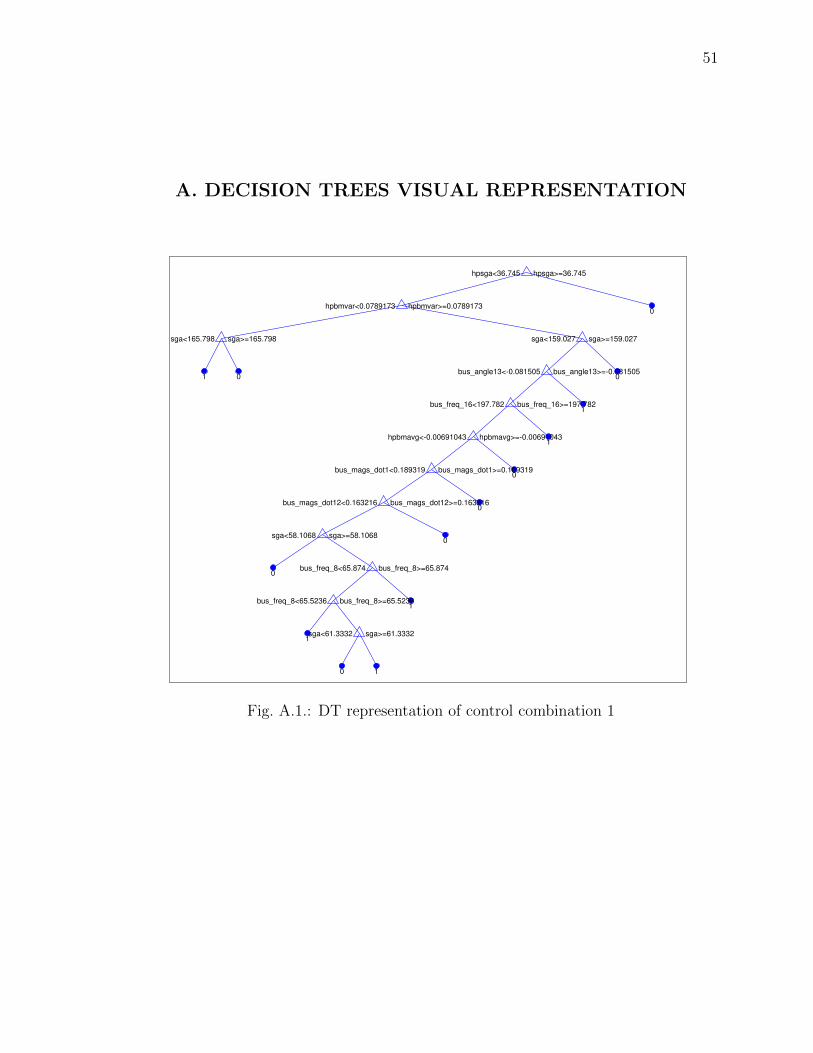
51

A. DECISION TREES VISUAL REPRESENTATION

0

1 0 0

1

1

0

0

0

0

1

1

0 1

hpsga<36.745

hpbmvar<0.0789173

sga<165.798 sga<159.027

bus_angle13<-0.081505

bus_freq_16<197.782

hpbmavg<-0.00691043

bus_mags_dot1<0.189319

bus_mags_dot12<0.163216

sga<58.1068

bus_freq_8<65.874

bus_freq_8<65.5236

sga<61.3332

hpsga>=36.745

hpbmvar>=0.0789173

sga>=165.798 sga>=159.027

bus_angle13>=-0.081505

bus_freq_16>=197.782

hpbmavg>=-0.00691043

bus_mags_dot1>=0.189319

bus_mags_dot12>=0.163216

sga>=58.1068

bus_freq_8>=65.874

bus_freq_8>=65.5236

sga>=61.3332

Fig. A.1.: DT representation of control combination 1

52

0

1

0

1

1

1

1

1 0

bus_mags1<0.96809

bus_angle3<26.647

bus_freq_9<127.58

hpbmvar<0.0789173

sga<61.7848

bmavg<0.891301

bus_mags7<0.49468

bus_freq_7<233.024

bus_mags1>=0.96809

bus_angle3>=26.647

bus_freq_9>=127.58

hpbmvar>=0.0789173

sga>=61.7848

bmavg>=0.891301

bus_mags7>=0.49468

bus_freq_7>=233.024

Fig. A.2.: DT representation of control combination 2

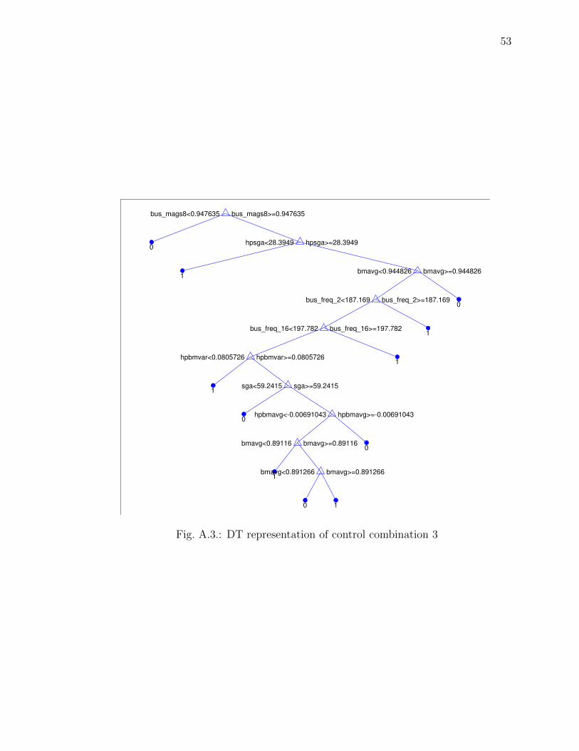
53

0

1

0

1

1

1

0

0

1

0 1

bus_mags8<0.947635

hpsga<28.3949

bmavg<0.944826

bus_freq_2<187.169

bus_freq_16<197.782

hpbmvar<0.0805726

sga<59.2415

hpbmavg<-0.00691043

bmavg<0.89116

bmavg<0.891266

bus_mags8>=0.947635

hpsga>=28.3949

bmavg>=0.944826

bus_freq_2>=187.169

bus_freq_16>=197.782

hpbmvar>=0.0805726

sga>=59.2415

hpbmavg>=-0.00691043

bmavg>=0.89116

bmavg>=0.891266

Fig. A.3.: DT representation of control combination 3