Embed Size (px)
Citation preview

Applied Statistics and Probability
Applied Statistics and Probability
Gilbert Ritschard
Department of economics, University of Genevahttp://mephisto.unige.ch
Master in International Trading,Commodity Finance and Shipping
18/9/2013gr 1/150
Applied Statistics and Probability
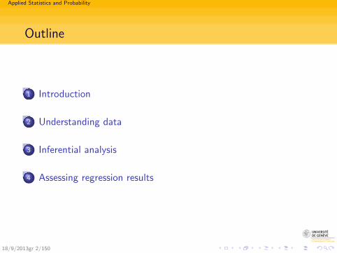
Outline
1 Introduction
2 Understanding data
3 Inferential analysis
4 Assessing regression results
18/9/2013gr 2/150
Applied Statistics and Probability
Introduction
Outline
1 Introduction
2 Understanding data
3 Inferential analysis
4 Assessing regression results
18/9/2013gr 3/150
Applied Statistics and Probability
Introduction
Why do we need statistics?
Section outline
1 IntroductionWhy do we need statistics?Illustrative examples: How is Crude Oil Price related toeconomic fundamentals?
18/9/2013gr 4/150
Applied Statistics and Probability
Introduction
Why do we need statistics?
Why statistics?
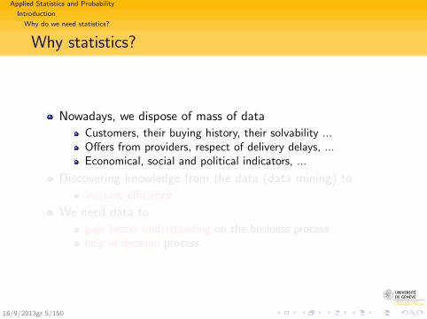
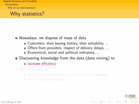
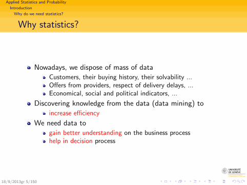
Nowadays, we dispose of mass of data
Customers, their buying history, their solvability ...Offers from providers, respect of delivery delays, ...Economical, social and political indicators, ...
Discovering knowledge from the data (data mining) to
increase efficiency
We need data to
gain better understanding on the business processhelp in decision process
18/9/2013gr 5/150
Applied Statistics and Probability
Introduction
Why do we need statistics?
Why statistics?
Nowadays, we dispose of mass of data
Customers, their buying history, their solvability ...Offers from providers, respect of delivery delays, ...Economical, social and political indicators, ...
Discovering knowledge from the data (data mining) to
increase efficiency
We need data to
gain better understanding on the business processhelp in decision process
18/9/2013gr 5/150
Applied Statistics and Probability
Introduction
Why do we need statistics?
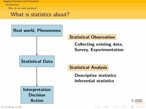
What is statistics about?
Real world, Phenomena
Statistical Observation
Collecting existing data,Survey, Experimentation
Statistical Data
Statistical Analysis
Descriptive statisticsInferential statistics
InterpretationDecisionAction
18/9/2013gr 6/150

Applied Statistics and Probability
Introduction
Why do we need statistics?
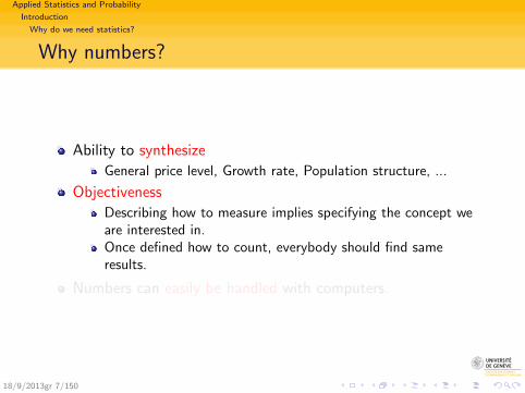
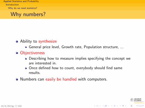
Why numbers?
Ability to synthesize
General price level, Growth rate, Population structure, ...
Objectiveness
Describing how to measure implies specifying the concept weare interested in.Once defined how to count, everybody should find sameresults.
Numbers can easily be handled with computers.
18/9/2013gr 7/150
Applied Statistics and Probability
Introduction
Why do we need statistics?
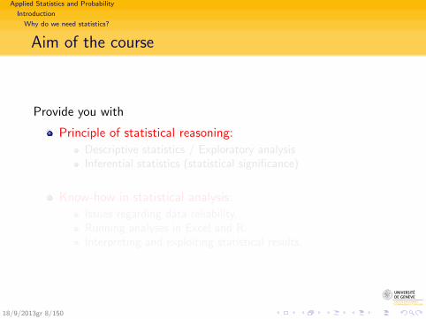
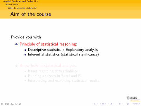
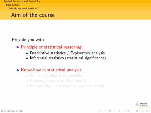
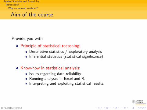
Aim of the course
Provide you with
Principle of statistical reasoning:
Descriptive statistics / Exploratory analysisInferential statistics (statistical significance)
Know-how in statistical analysis:
Issues regarding data reliability.Running analyses in Excel and R.Interpreting and exploiting statistical results.
18/9/2013gr 8/150
Applied Statistics and Probability
Introduction
Why do we need statistics?
Aim of the course
Provide you with
Principle of statistical reasoning:
Descriptive statistics / Exploratory analysisInferential statistics (statistical significance)
Know-how in statistical analysis:
Issues regarding data reliability.Running analyses in Excel and R.Interpreting and exploiting statistical results.
18/9/2013gr 8/150
Applied Statistics and Probability
Introduction
Illustrative examples: How is Crude Oil Price related to economic fundamentals?
Section outline
1 IntroductionWhy do we need statistics?Illustrative examples: How is Crude Oil Price related toeconomic fundamentals?
18/9/2013gr 9/150

Applied Statistics and Probability
Introduction
Illustrative examples: How is Crude Oil Price related to economic fundamentals?
Sources of the illustrative data
Crude Oil prices
US Energy Information Administration EIA:http://www.eia.gov
Spot prices Petroleum and other liquidshttp://www.eia.gov/dnav/pet/pet_pri_spt_s1_d.htm
We extracted the Crude Oil RWTC price (Cushing, OK WTISpot Price FOB) in Dollars per Barrel.
US Macro data
From the World Economic Outlook database of theInternational Monetary Fund (IMF)http://www.imf.org/external/pubs/ft/weo/2013/01/weodata/download.aspx
18/9/2013gr 10/150

Applied Statistics and Probability
Introduction
Illustrative examples: How is Crude Oil Price related to economic fundamentals?
Data preparation
Data from the World Economic Outlook (WEO) are yearlydata with the values of the variables displayed in rows.
Spot prices are daily data displayed in columns.
Preparation steps:
Transpose the WEO data (rows → columns)Aggregate the daily crude oil prices into yearly data
For this illustration, we just keep the first valid price each yearAlternatives: Price at any other date, yearly mean price, ...
Merge the two data sets by year.
18/9/2013gr 11/150
Applied Statistics and Probability
Introduction
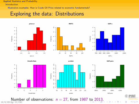
Illustrative examples: How is Crude Oil Price related to economic fundamentals?
Exploring the data: Distributions
price.cr
price.cr
Fre
quen
cy
−1.0 −0.5 0.0 0.5
01
23
45
67
RWTC
RWTC
Fre
quen
cy
20 40 60 80 1000
24
68
10
GDP.c
GDP.c
Fre
quen
cy
7000 8000 9000 10000 12000 14000
01
23
45
6
Growth.Rate
Growth.Rate
Fre
quen
cy
−4 −2 0 2 4
01
23
45
6
p.index
p.index
Fre
quen
cy
60 70 80 90 100 110 120
0.0
0.5
1.0
1.5
2.0
2.5
3.0
GDP.pers
GDP.pers
Fre
quen
cy30000 34000 38000 42000
02
46
8
Number of observations: n = 27, from 1987 to 2013.18/9/2013gr 12/150
Applied Statistics and Probability
Introduction
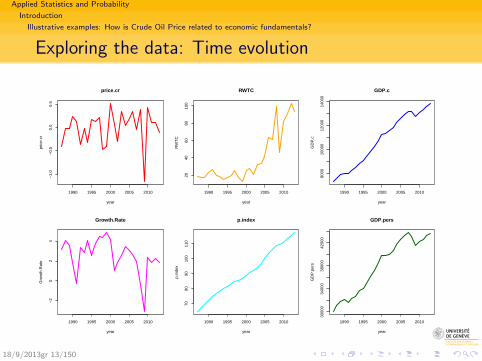
Illustrative examples: How is Crude Oil Price related to economic fundamentals?
Exploring the data: Time evolution
1990 1995 2000 2005 2010
−1.
0−
0.5
0.0
0.5
price.cr
year
pric
e.cr
1990 1995 2000 2005 2010
2040
6080
100
RWTC
year
RW
TC
1990 1995 2000 2005 2010
8000
1000
012
000
1400
0
GDP.c
year
GD
P.c
1990 1995 2000 2005 2010
−2
02
4
Growth.Rate
year
Gro
wth
.Rat
e
1990 1995 2000 2005 2010
7080
9010
011
0
p.index
year
p.in
dex
1990 1995 2000 2005 201030
000
3400
038
000
4200
0
GDP.pers
year
GD
P.p
ers
18/9/2013gr 13/150
Applied Statistics and Probability
Introduction
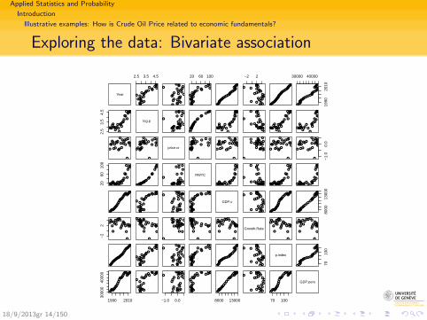
Illustrative examples: How is Crude Oil Price related to economic fundamentals?
Exploring the data: Bivariate association
Year
2.5 3.5 4.5
●●● ●●●●
●●● ●●● ●●● ●●
● ●●●● ●●●●
● ●●●●● ●● ●●●●●
●●● ●●●●● ●● ●●●●
20 60 100
●●●●●●●
●●●●●● ●●● ●●
● ●●●● ●● ●●
●●●●●●
●●●●●●●●●
●●●●●●
●●●●●
●
−2 2
● ●●●● ●● ●● ●●●●●●●● ●●●●●● ●●●●
●●●●●
●●●●●●●●●●●●
●●●●●●●
●●●
30000 40000
1990
2010
●●●●●●
●●●●●●●●●
●●●●●●
●●●●●
●
2.5
3.5
4.5
●●●●●
●●●●●●
●
●
●●●
●●●
●●
●
●
●●●●
log.p
● ●●●
●
● ●●
●●●
●
●
●●●
●●●
●●
●
●
●●●●
●●●●●
●●●●●●
●
●
●●●
●●●
●●
●
●
●● ●●
●●●●●
●●●●●●
●
●
●●●
●●●
●●
●
●
●●●●
● ●●●
●
●●●
●●
●
●
●
●●●
● ●●
●●
●
●
●●●●
●●●●●
●●●●●●
●
●
●●●
●●●
●●
●
●
●●●●
●●●●
●
●●●●●
●
●
●
●●●
●●●
●●
●
●
●●●●
●
●●
●●
●
●
●
●●●
●●
●
●
●
●
●●●
●
●
●
●
●●●
●
●●
●●
●
●
●
●●●
●●
●
●
●
●
●●
●
●
●
●
●
●●●
price.cr ●
●●
●●
●
●
●
●●●
●●
●
●
●
●
●●
●
●
●
●
●
● ●●
●
●●
●●
●
●
●
●●●
●●
●
●
●
●
●●●
●
●
●
●
●●●
●
●●
●●
●
●
●
● ●●
●●
●
●
●
●
●●
●
●
●
●
●
●●●
●
●●
●●
●
●
●
●●●
●●
●
●
●
●
●●●
●
●
●
●
●●●
−1.
00.
0
●
●●
●●
●
●
●
●●●
●●
●
●
●
●
●●●
●
●
●
●
●●●
2060
100
●●●●●●●●●
●●●●
●●●●●
●
●●
●
●
●●●●
●●●●●
●●●●●●
●●●●●
●●●
●●
●
●
●●●
●
● ●●●●
● ●● ●●●
●●●●
●●●
●
●●
●
●
●●●
●
RWTC
●●●●●●●●●
●●●●
●●●●●
●
●●
●
●
●●●●
● ●●●●
●● ●● ●●●●●●
●● ●●
●●
●
●
●●●
●
●●●●●●●●●
●●●●●●●
●●●
●●
●
●
●●●●
●●●●●●●●●
●●
●●●●●
●●●
●●
●
●
●●●●
●●●●●
●●●●
●●●●●●●
●●●
●●●●●●●
●
●●● ●●●●
●●●●
●●
●●● ●●● ●● ●
● ●●●●
● ●●●●● ●● ●●●
●●
●●● ●●●●● ●
● ●●●●
●●●●●●●●●●●
●●
●●● ●●● ●● ●
● ●● ●●
GDP.c
● ●●●● ●● ●● ●●●●
●●●●●●●●●
● ●●●●
●●●●●●
●●●●●●●●●●
●●●●●●
●●●●
●
8000
1300
0
●●●●●●●
●●●
●●
●●●●
●●●●●●●●●●
●
−2
2
●●●
●
●
●●
●
●
●●●
●●
●●●●●●
●
●
●
●●●●
●●●
●
●
●●
●
●
●●●
●●
●●
●●● ●
●
●
●
●●●●
●●●
●
●
●●
●
●
●●●
●●
●●
●●●●
●
●
●
●●●●
●●●
●
●
●●
●
●
●●●
●●
●●
●●● ●
●
●
●
●● ●●
●●●
●
●
●●
●
●
●●●
●●
●●●●●●
●
●
●
●●●●
Growth.Rate
●●●
●
●
●●
●
●
●●●●●
●●●●●●
●
●
●
●●●●
●●●
●
●
●●
●
●
●●●
●●
●●●
●●●●
●
●
●●●●
●●●●
●●●●
●●●●●
●●●●
●●●●
●●●●●
●
●●● ●●●●
●●● ●●● ●●● ●●
●●●
●● ●●●●
● ●●●●● ●● ●●●●●
●●● ●●●
●● ●● ●●●●
●●●●●●●
●●●●●● ●●● ●●
●●●
●● ●● ●●
●●●●●●
●●●●●●●●●
●●●●●●●●●●●
●
● ●●●● ●● ●● ●●●●●●●● ●●
●●●● ●●●●
p.index
7010
0
●●●●●●
●●●●●●●●●
●●●●●●●●●
●●●
1990 2010
3000
040
000
●●●●●●
●●●
●●●●●●●
●●●●
●●●●
●●●
●●● ●●●●
●●●
●●
●●●● ●
●● ●● ●● ●●●●
−1.0 0.0
●●● ●●● ●
● ●●●
●●
●●● ●●
●●● ●● ●●●
●
●●●●●●●●●●●
●●
●●● ●●
● ●● ●● ●● ●●
8000 13000
●●●●●●
●●●
●●●
●●●●
●●●●●●●●
●●●
●●
●●● ●●●●
●●●●
●●●●●
●●●●● ●●●●
70 100
●●●●●●
●●●●●●●●●●
●●●●●●
●●●●
●
GDP.pers
18/9/2013gr 14/150
Applied Statistics and Probability
Introduction
Illustrative examples: How is Crude Oil Price related to economic fundamentals?
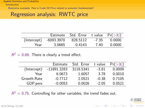
Regression analysis: RWTC price
Estimate Std. Error t value Pr(>|t|)(Intercept) -6093.3970 828.5112 -7.35 0.0000
Year 3.0665 0.4143 7.40 0.0000
R2 = 0.69. There is clearly a trend effect.
Estimate Std. Error t value Pr(>|t|)(Intercept) -11891.3283 3118.5341 -3.81 0.0009
Year 6.0673 1.6057 3.78 0.0010Growth.Rate -0.7712 2.0521 -0.38 0.7105
GDP.pers -0.0053 0.0026 -2.05 0.0521
R2 = 0.75. Controlling for other variables, the trend fades out.
18/9/2013gr 15/150
Applied Statistics and Probability
Introduction
Illustrative examples: How is Crude Oil Price related to economic fundamentals?
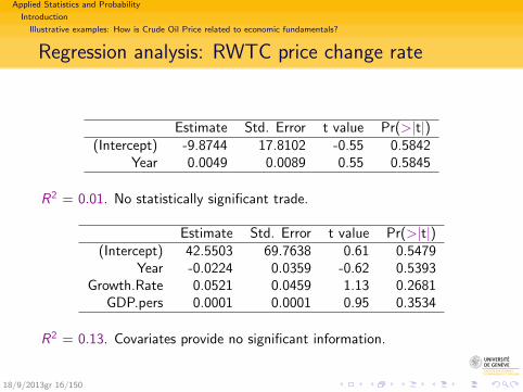
Regression analysis: RWTC price change rate
Estimate Std. Error t value Pr(>|t|)(Intercept) -9.8744 17.8102 -0.55 0.5842
Year 0.0049 0.0089 0.55 0.5845
R2 = 0.01. No statistically significant trade.
Estimate Std. Error t value Pr(>|t|)(Intercept) 42.5503 69.7638 0.61 0.5479
Year -0.0224 0.0359 -0.62 0.5393Growth.Rate 0.0521 0.0459 1.13 0.2681
GDP.pers 0.0001 0.0001 0.95 0.3534
R2 = 0.13. Covariates provide no significant information.
18/9/2013gr 16/150
Applied Statistics and Probability
Understanding data
Outline
1 Introduction
2 Understanding data
3 Inferential analysis
4 Assessing regression results
18/9/2013gr 17/150
Applied Statistics and Probability
Understanding data
The data
Section outline
2 Understanding dataThe dataSoftwareExploratory univariate statistics
ObjectiveSummary tables and graphicsSummary numbers: central values, dispersion, ...Detecting and filtering out outliersModeling and comparing data distributions
Bivariate dataCross tabulationPlotting bivariate data: stacked bars, scatter plotMeasuring association
Linear RegressionMultiple Regression
Linearity in parameters and non linear relationsAbout non linear relations18/9/2013gr 18/150
Applied Statistics and Probability
Understanding data
The data
Sources of dataStatistical observation
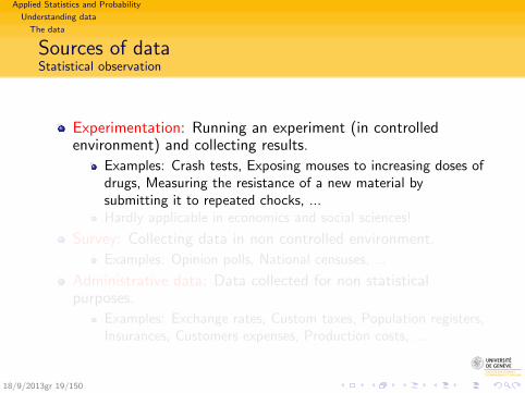
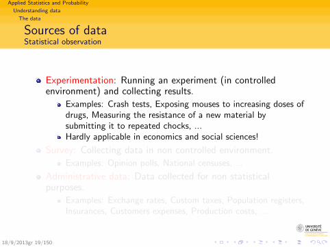
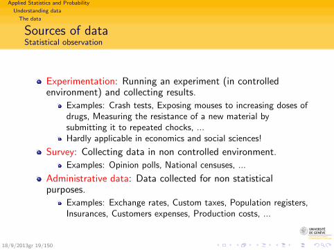
Experimentation: Running an experiment (in controlledenvironment) and collecting results.
Examples: Crash tests, Exposing mouses to increasing doses ofdrugs, Measuring the resistance of a new material bysubmitting it to repeated chocks, ...Hardly applicable in economics and social sciences!
Survey: Collecting data in non controlled environment.
Examples: Opinion polls, National censuses, ...
Administrative data: Data collected for non statisticalpurposes.
Examples: Exchange rates, Custom taxes, Population registers,Insurances, Customers expenses, Production costs, ...
18/9/2013gr 19/150
Applied Statistics and Probability
Understanding data
The data
Sources of dataStatistical observation
Experimentation: Running an experiment (in controlledenvironment) and collecting results.
Examples: Crash tests, Exposing mouses to increasing doses ofdrugs, Measuring the resistance of a new material bysubmitting it to repeated chocks, ...Hardly applicable in economics and social sciences!
Survey: Collecting data in non controlled environment.
Examples: Opinion polls, National censuses, ...
Administrative data: Data collected for non statisticalpurposes.
Examples: Exchange rates, Custom taxes, Population registers,Insurances, Customers expenses, Production costs, ...
18/9/2013gr 19/150
Applied Statistics and Probability
Understanding data
The data
Sampled and exhaustive data
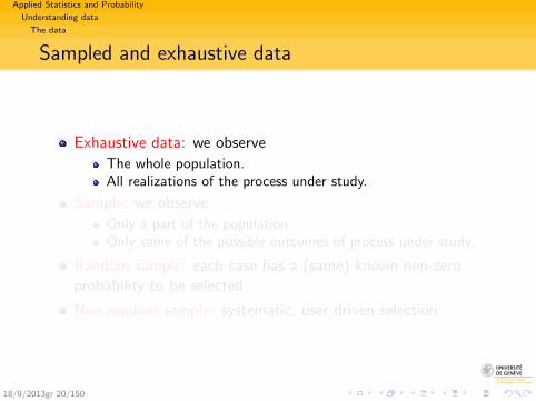
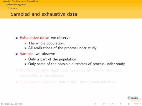
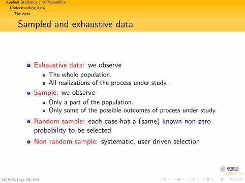
Exhaustive data: we observe
The whole population.All realizations of the process under study.
Sample: we observe
Only a part of the population.Only some of the possible outcomes of process under study.
Random sample: each case has a (same) known non-zeroprobability to be selected
Non random sample: systematic, user driven selection
18/9/2013gr 20/150
Applied Statistics and Probability
Understanding data
The data
Sampled and exhaustive data
Exhaustive data: we observe
The whole population.All realizations of the process under study.
Sample: we observe
Only a part of the population.Only some of the possible outcomes of process under study.
Random sample: each case has a (same) known non-zeroprobability to be selected
Non random sample: systematic, user driven selection
18/9/2013gr 20/150
Applied Statistics and Probability
Understanding data
The data
Data reliability and relevance
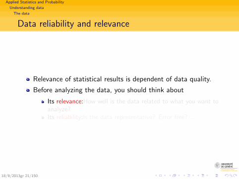
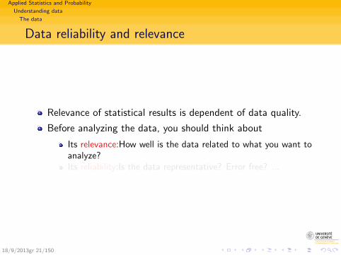
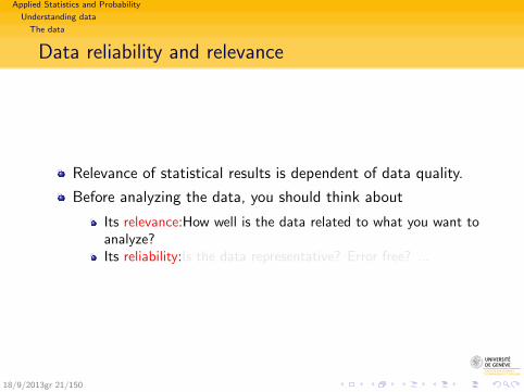
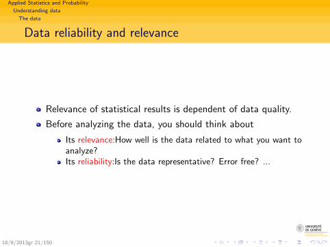
Relevance of statistical results is dependent of data quality.
Before analyzing the data, you should think about
Its relevance:How well is the data related to what you want toanalyze?Its reliability:Is the data representative? Error free? ...
18/9/2013gr 21/150
Applied Statistics and Probability
Understanding data
The data
Data reliability and relevance
Relevance of statistical results is dependent of data quality.
Before analyzing the data, you should think about
Its relevance:How well is the data related to what you want toanalyze?Its reliability:Is the data representative? Error free? ...
18/9/2013gr 21/150
Applied Statistics and Probability
Understanding data
The data
Statistical objects and attributes
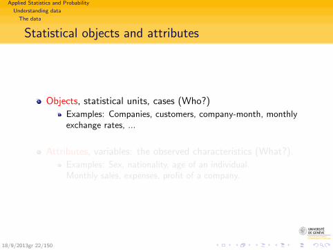
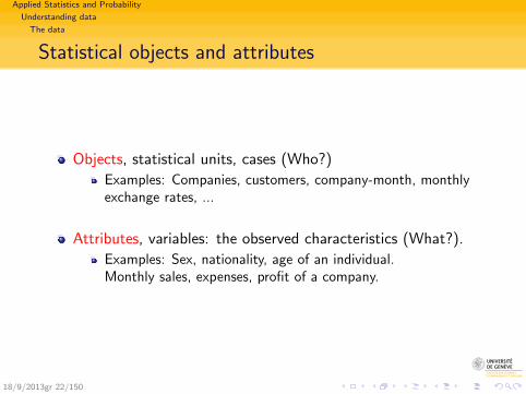
Objects, statistical units, cases (Who?)
Examples: Companies, customers, company-month, monthlyexchange rates, ...
Attributes, variables: the observed characteristics (What?).
Examples: Sex, nationality, age of an individual.Monthly sales, expenses, profit of a company.
18/9/2013gr 22/150
Applied Statistics and Probability
Understanding data
The data
Statistical objects and attributes
Objects, statistical units, cases (Who?)
Examples: Companies, customers, company-month, monthlyexchange rates, ...
Attributes, variables: the observed characteristics (What?).
Examples: Sex, nationality, age of an individual.Monthly sales, expenses, profit of a company.
18/9/2013gr 22/150
Applied Statistics and Probability
Understanding data
The data
Measurement levels
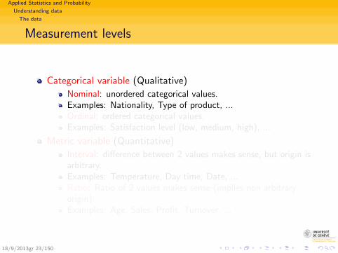
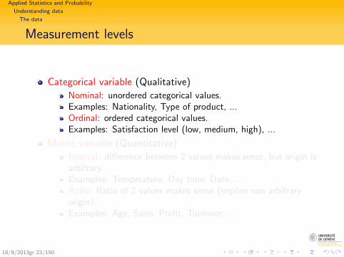
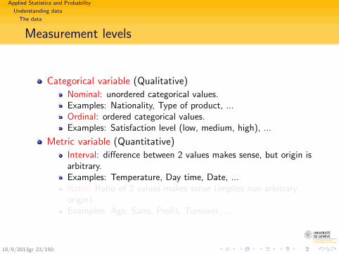
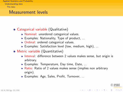
Categorical variable (Qualitative)
Nominal: unordered categorical values.Examples: Nationality, Type of product, ...Ordinal: ordered categorical values.Examples: Satisfaction level (low, medium, high), ...
Metric variable (Quantitative)
Interval: difference between 2 values makes sense, but origin isarbitrary.Examples: Temperature, Day time, Date, ...Ratio: Ratio of 2 values makes sense (implies non arbitraryorigin).Examples: Age, Sales, Profit, Turnover, ...
18/9/2013gr 23/150
Applied Statistics and Probability
Understanding data
The data
Measurement levels
Categorical variable (Qualitative)
Nominal: unordered categorical values.Examples: Nationality, Type of product, ...Ordinal: ordered categorical values.Examples: Satisfaction level (low, medium, high), ...
Metric variable (Quantitative)
Interval: difference between 2 values makes sense, but origin isarbitrary.Examples: Temperature, Day time, Date, ...Ratio: Ratio of 2 values makes sense (implies non arbitraryorigin).Examples: Age, Sales, Profit, Turnover, ...
18/9/2013gr 23/150
Applied Statistics and Probability
Understanding data
The data
Database
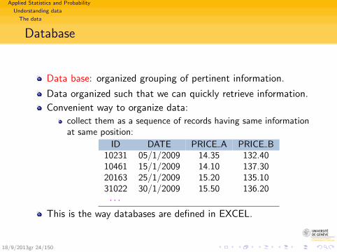
Data base: organized grouping of pertinent information.
Data organized such that we can quickly retrieve information.
Convenient way to organize data:
collect them as a sequence of records having same informationat same position:
ID DATE PRICE A PRICE B10231 05/1/2009 14.35 132.4010461 15/1/2009 14.10 137.3020163 25/1/2009 15.20 135.1031022 30/1/2009 15.50 136.20· · ·
This is the way databases are defined in EXCEL.
18/9/2013gr 24/150
Applied Statistics and Probability
Understanding data
The data
Individual and Aggregated Data
Individual data
Each record (case, observation) corresponds to the finestobservation unit.Usually each record has the same weight.
Aggregated data
Each record summarizes the data of a group of records.The aggregated records have different weights reflecting thenumber of cases represented.
Tabulating data results in aggregated data.
Aggregating
more concise (readable) form.But, loss of some information.
,
18/9/2013gr 25/150
Applied Statistics and Probability
Understanding data
The data
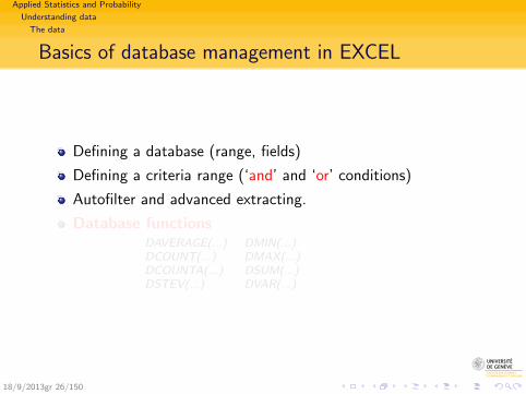
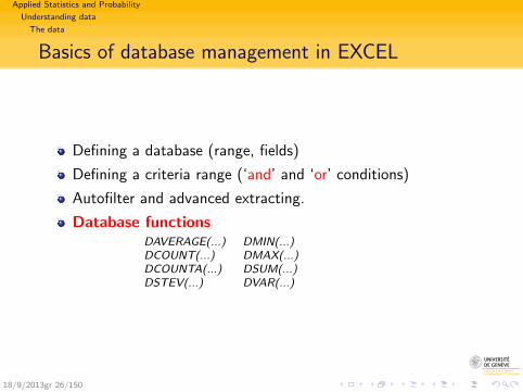
Basics of database management in EXCEL
Defining a database (range, fields)
Defining a criteria range (‘and’ and ‘or’ conditions)
Autofilter and advanced extracting.
Database functionsDAVERAGE(...) DMIN(...)DCOUNT(...) DMAX(...)DCOUNTA(...) DSUM(...)DSTEV(...) DVAR(...)
18/9/2013gr 26/150
Applied Statistics and Probability
Understanding data
The data
Basics of database management in EXCEL
Defining a database (range, fields)
Defining a criteria range (‘and’ and ‘or’ conditions)
Autofilter and advanced extracting.
Database functionsDAVERAGE(...) DMIN(...)DCOUNT(...) DMAX(...)DCOUNTA(...) DSUM(...)DSTEV(...) DVAR(...)
18/9/2013gr 26/150
Applied Statistics and Probability
Understanding data
Software
Section outline
2 Understanding dataThe dataSoftwareExploratory univariate statistics
ObjectiveSummary tables and graphicsSummary numbers: central values, dispersion, ...Detecting and filtering out outliersModeling and comparing data distributions
Bivariate dataCross tabulationPlotting bivariate data: stacked bars, scatter plotMeasuring association
Linear RegressionMultiple Regression
Linearity in parameters and non linear relationsAbout non linear relations18/9/2013gr 27/150

Applied Statistics and Probability
Understanding data
Software
Software
We need software for
Data managementstatistical analysis
There are plenty of statistical and data management packages.
For the course, we’ll be using two of them:
Excel (from Microsoft Office Suite): Spreadsheet with limitedstatistical possibilitiesR: Free statistical and graphical environment (programming)
We propose
Introduction to Excel and programming with Visual basic forExcel (VBA)Introduction to R (using R-Studio shell)
18/9/2013gr 28/150
Applied Statistics and Probability
Understanding data
Exploratory univariate statistics
Section outline
2 Understanding dataThe dataSoftwareExploratory univariate statistics
ObjectiveSummary tables and graphicsSummary numbers: central values, dispersion, ...Detecting and filtering out outliersModeling and comparing data distributions
Bivariate dataCross tabulationPlotting bivariate data: stacked bars, scatter plotMeasuring association
Linear RegressionMultiple Regression
Linearity in parameters and non linear relationsAbout non linear relations18/9/2013gr 29/150
Applied Statistics and Probability
Understanding data
Exploratory univariate statistics
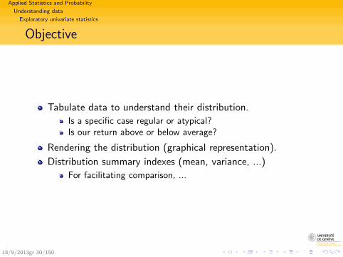
Objective
Tabulate data to understand their distribution.
Is a specific case regular or atypical?Is our return above or below average?
Rendering the distribution (graphical representation).
Distribution summary indexes (mean, variance, ...)
For facilitating comparison, ...
18/9/2013gr 30/150
Applied Statistics and Probability
Understanding data
Exploratory univariate statistics
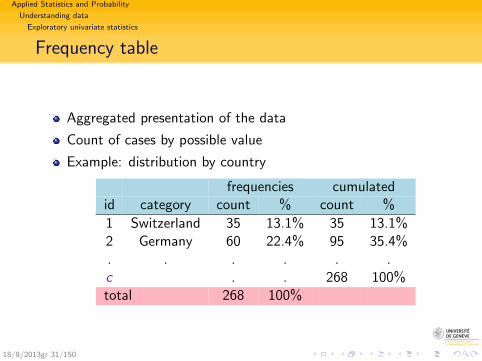
Frequency table
Aggregated presentation of the data
Count of cases by possible value
Example: distribution by country
frequencies cumulatedid category count % count %
1 Switzerland 35 13.1% 35 13.1%2 Germany 60 22.4% 95 35.4%. . . . . .c . . 268 100%total 268 100%
18/9/2013gr 31/150
Applied Statistics and Probability
Understanding data
Exploratory univariate statistics
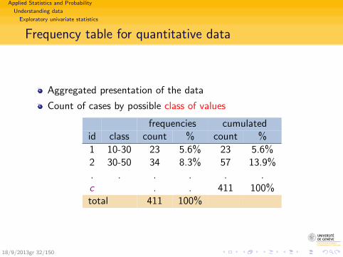
Frequency table for quantitative data
Aggregated presentation of the data
Count of cases by possible class of values
frequencies cumulatedid class count % count %
1 10-30 23 5.6% 23 5.6%2 30-50 34 8.3% 57 13.9%. . . . . .c . . 411 100%total 411 100%
18/9/2013gr 32/150
Applied Statistics and Probability
Understanding data
Exploratory univariate statistics
Building summary tables in R and Excel
In R you use the summary or table functions.
In Excel you use the tool named Pivot Table
Select the data range (with column headings)Click on Pivot Table (Insert menu tab in Excel 2007)
From the Pivot Table Field List, drag variable name
Once to the Row field of the Pivot TableOnce to the Data area of the Pivot Table
If necessary, set the used summary value to ‘count’(contextual menu from the cell above ‘Category’)
For a continuous variable (many different values)
You should first create the class values!
18/9/2013gr 33/150
Applied Statistics and Probability
Understanding data
Exploratory univariate statistics
Graphics
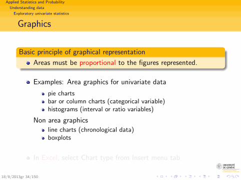
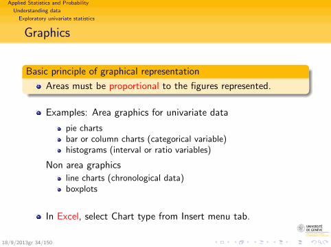
Basic principle of graphical representation
Areas must be proportional to the figures represented.
Examples: Area graphics for univariate data
pie chartsbar or column charts (categorical variable)histograms (interval or ratio variables)
Non area graphics
line charts (chronological data)boxplots
In Excel, select Chart type from Insert menu tab.
18/9/2013gr 34/150
Applied Statistics and Probability
Understanding data
Exploratory univariate statistics
Graphics
Basic principle of graphical representation
Areas must be proportional to the figures represented.
Examples: Area graphics for univariate data
pie chartsbar or column charts (categorical variable)histograms (interval or ratio variables)
Non area graphics
line charts (chronological data)boxplots
In Excel, select Chart type from Insert menu tab.
18/9/2013gr 34/150
Applied Statistics and Probability
Understanding data
Exploratory univariate statistics
Histogram
Histogram
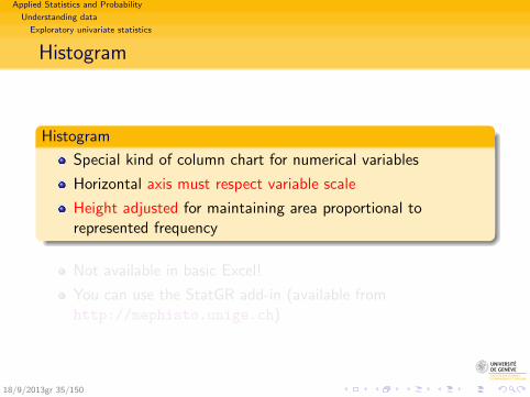
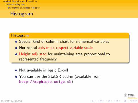
Special kind of column chart for numerical variables
Horizontal axis must respect variable scale
Height adjusted for maintaining area proportional torepresented frequency
Not available in basic Excel!
You can use the StatGR add-in (available fromhttp://mephisto.unige.ch)
18/9/2013gr 35/150
Applied Statistics and Probability
Understanding data
Exploratory univariate statistics
Histogram
Histogram
Special kind of column chart for numerical variables
Horizontal axis must respect variable scale
Height adjusted for maintaining area proportional torepresented frequency
Not available in basic Excel!
You can use the StatGR add-in (available fromhttp://mephisto.unige.ch)
18/9/2013gr 35/150
Applied Statistics and Probability
Understanding data
Exploratory univariate statistics
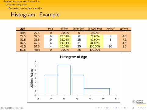
Histogram: Example
Age freq % freq cum freq % cum freq range heightless 27.5 0 0.00% 0 0.00%27.5 32.5 6 24.00% 6 24.00% 5 4.832.5 37.5 9 36.00% 15 60.00% 5 7.237.5 42.5 6 24.00% 21 84.00% 5 4.842.5 52.5 4 16.00% 25 100.00% 10 1.652.5 more 0 0.00% 25 100.00%
5
6
7
8
ange
Histogram of Age
0
1
2
3
4
5
25 30 35 40 45 50 55
100
freq
/ ra
18/9/2013gr 36/150
Applied Statistics and Probability
Understanding data
Exploratory univariate statistics
‘Descriptive Statistics’ from Excel
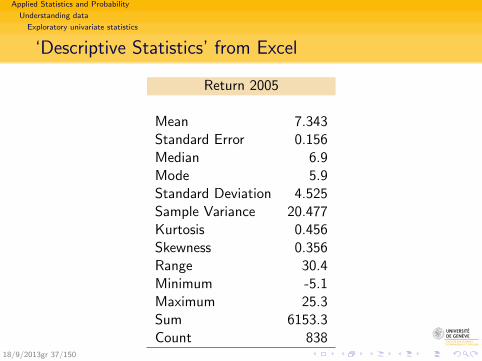
Return 2005
Mean 7.343Standard Error 0.156Median 6.9Mode 5.9Standard Deviation 4.525Sample Variance 20.477Kurtosis 0.456Skewness 0.356Range 30.4Minimum -5.1Maximum 25.3Sum 6153.3Count 838
18/9/2013gr 37/150
Applied Statistics and Probability
Understanding data
Exploratory univariate statistics
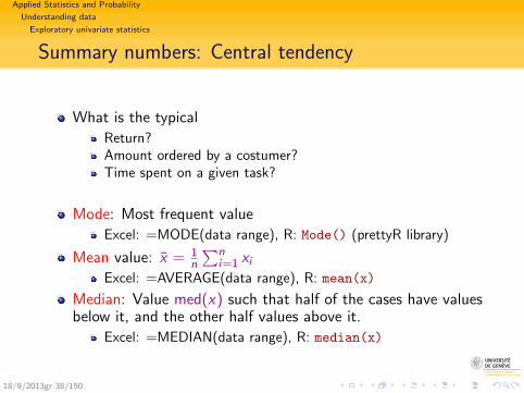
Summary numbers: Central tendency
What is the typical
Return?Amount ordered by a costumer?Time spent on a given task?
Mode: Most frequent value
Excel: =MODE(data range), R: Mode() (prettyR library)
Mean value: x = 1n
∑ni=1 xi
Excel: =AVERAGE(data range), R: mean(x)
Median: Value med(x) such that half of the cases have valuesbelow it, and the other half values above it.
Excel: =MEDIAN(data range), R: median(x)
18/9/2013gr 38/150
Applied Statistics and Probability
Understanding data
Exploratory univariate statistics
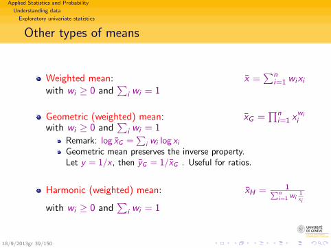
Other types of means
Weighted mean: x =∑n
i=1 wixiwith wi ≥ 0 and
∑i wi = 1
Geometric (weighted) mean: xG =∏n
i=1 xwii
with wi ≥ 0 and∑
i wi = 1
Remark: log xG =∑
i wi log xiGeometric mean preserves the inverse property.Let y = 1/x , then yG = 1/xG . Useful for ratios.
Harmonic (weighted) mean: xH = 1∑ni=1 wi
1xi
with wi ≥ 0 and∑
i wi = 1
18/9/2013gr 39/150
Applied Statistics and Probability
Understanding data
Exploratory univariate statistics
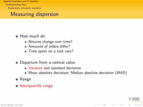
Measuring dispersion
How much do
Returns change over time?Amounts of orders differ?Time spent on a task vary?
Departure from a central value
Variance and standard deviationMean absolute deviation, Median absolute deviation (MAD)
Range
Interquartile range
18/9/2013gr 40/150
Applied Statistics and Probability
Understanding data
Exploratory univariate statistics
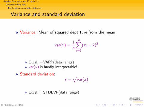
Variance and standard deviation
Variance: Mean of squared departure from the mean
var(x) =1
n
n∑i=1
(xi − x)2
Excel: =VARP(data range)var(x) is hardly interpretable!
Standard deviation:s =
√var(x)
Excel: =STDEVP(data range)
18/9/2013gr 41/150
Applied Statistics and Probability
Understanding data
Exploratory univariate statistics
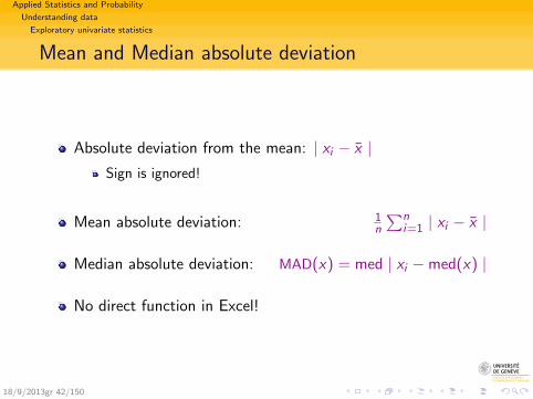
Mean and Median absolute deviation
Absolute deviation from the mean: | xi − x |Sign is ignored!
Mean absolute deviation: 1n
∑ni=1 | xi − x |
Median absolute deviation: MAD(x) = med | xi −med(x) |
No direct function in Excel!
18/9/2013gr 42/150
Applied Statistics and Probability
Understanding data
Exploratory univariate statistics
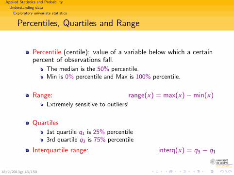
Percentiles, Quartiles and Range
Percentile (centile): value of a variable below which a certainpercent of observations fall.
The median is the 50% percentile.Min is 0% percentile and Max is 100% percentile.
Range: range(x) = max(x)−min(x)
Extremely sensitive to outliers!
Quartiles
1st quartile q1 is 25% percentile3rd quartile q3 is 75% percentile
Interquartile range: interq(x) = q3 − q1
18/9/2013gr 43/150
Applied Statistics and Probability
Understanding data
Exploratory univariate statistics
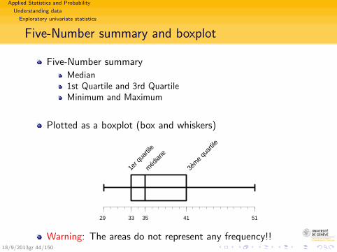
Five-Number summary and boxplot
Five-Number summary
Median1st Quartile and 3rd QuartileMinimum and Maximum
Plotted as a boxplot (box and whiskers)
1er q
uarti
le
29 5135
3èm
e qu
artile
méd
iane
33 41
Warning: The areas do not represent any frequency!!18/9/2013gr 44/150
Applied Statistics and Probability
Understanding data
Exploratory univariate statistics
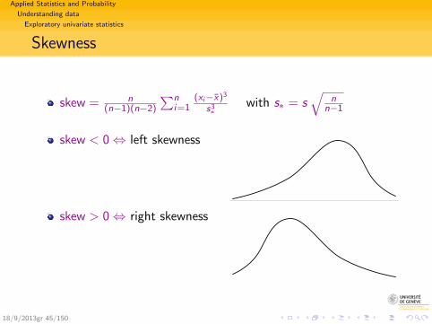
Skewness
skew = n(n−1)(n−2)
∑ni=1
(xi−x)3
s3∗
with s∗ = s√
nn−1
skew < 0⇔ left skewness
skew > 0⇔ right skewness
18/9/2013gr 45/150
Applied Statistics and Probability
Understanding data
Exploratory univariate statistics
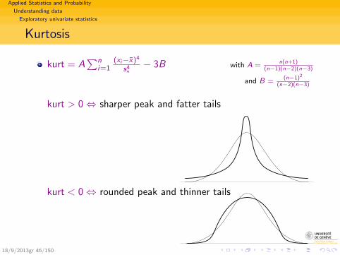
Kurtosis
kurt = A∑n
i=1(xi−x)4
s4∗− 3B with A = n(n+1)
(n−1)(n−2)(n−3)
and B = (n−1)2
(n−2)(n−3)
kurt > 0⇔ sharper peak and fatter tails
kurt < 0⇔ rounded peak and thinner tails
18/9/2013gr 46/150
Applied Statistics and Probability
Understanding data
Exploratory univariate statistics
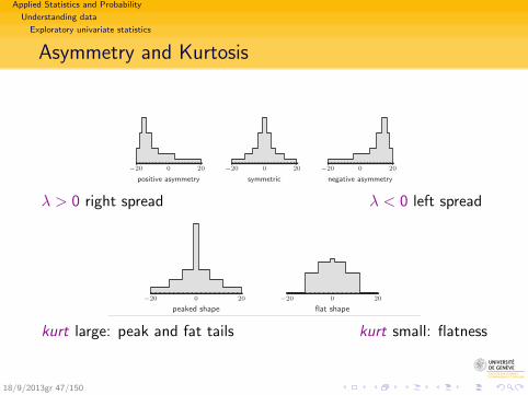
Asymmetry and Kurtosis
−20 0 20
positive asymmetry
−20 0 20
symmetric
−20 0 20
negative asymmetry
λ > 0 right spread λ < 0 left spread
−20 0 20
peaked shape
−20 0 20
flat shape
kurt large: peak and fat tails kurt small: flatness
18/9/2013gr 47/150
Applied Statistics and Probability
Understanding data
Exploratory univariate statistics
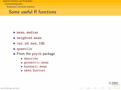
Some useful R functions
mean, median
weighted.mean
var, sd, mad, IQR
quantile
From the psych package
describe
geometric.mean
harmonic.mean
skew, kurtosi
18/9/2013gr 48/150
Applied Statistics and Probability
Understanding data
Exploratory univariate statistics
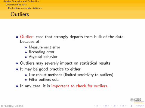
Outliers
Outlier: case that strongly departs from bulk of the databecause of
Measurement errorRecording errorAtypical behavior.
Outliers may severely impact on statistical results
It may be good practice to either
Use robust methods (limited sensitivity to outliers)Filter outliers out.
In any case, it is important to check for outliers.
18/9/2013gr 49/150
Applied Statistics and Probability
Understanding data
Exploratory univariate statistics
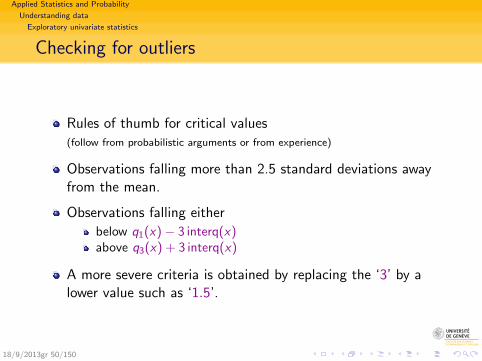
Checking for outliers
Rules of thumb for critical values(follow from probabilistic arguments or from experience)
Observations falling more than 2.5 standard deviations awayfrom the mean.
Observations falling either
below q1(x)− 3 interq(x)above q3(x) + 3 interq(x)
A more severe criteria is obtained by replacing the ‘3’ by alower value such as ‘1.5’.
18/9/2013gr 50/150
Applied Statistics and Probability
Understanding data
Exploratory univariate statistics
Modeling data distribution
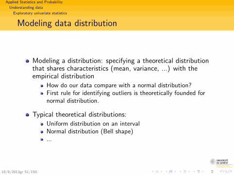
Modeling a distribution: specifying a theoretical distributionthat shares characteristics (mean, variance, ...) with theempirical distribution
How do our data compare with a normal distribution?First rule for identifying outliers is theoretically founded fornormal distribution.
Typical theoretical distributions:
Uniform distribution on an intervalNormal distribution (Bell shape)...
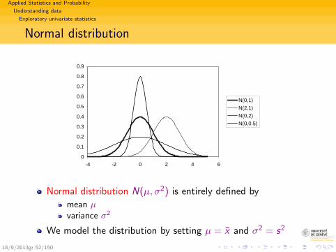
18/9/2013gr 51/150
Applied Statistics and Probability
Understanding data
Exploratory univariate statistics
Normal distribution
0
0.1
0.2
0.3
0.4
0.5
0.6
0.7
0.8
0.9
-4 -2 0 2 4 6
N(0,1)
N(2,1)
N(0,2)
N(0,0.5)
Normal distribution N(µ, σ2) is entirely defined by
mean µvariance σ2
We model the distribution by setting µ = x and σ2 = s2
18/9/2013gr 52/150

Applied Statistics and Probability
Understanding data
Exploratory univariate statistics
qq-plot for comparing distributions
43
48
53
mal
QQ-Plot of Age
23
28
33
38
23 28 33 38 43 48 53
Q n
orm
Q obs
qq-plot: quantile-quantile plot
k-th quantile of n values: kn -th percentile.
Plot empirical (observed) quantiles against quantiles ofmodeled distribution.You can generate qq-plot for normality with StatGR add-in.
18/9/2013gr 53/150
Applied Statistics and Probability
Understanding data
Bivariate data
Section outline
2 Understanding dataThe dataSoftwareExploratory univariate statistics
ObjectiveSummary tables and graphicsSummary numbers: central values, dispersion, ...Detecting and filtering out outliersModeling and comparing data distributions
Bivariate dataCross tabulationPlotting bivariate data: stacked bars, scatter plotMeasuring association
Linear RegressionMultiple Regression
Linearity in parameters and non linear relationsAbout non linear relations18/9/2013gr 54/150
Applied Statistics and Probability
Understanding data
Bivariate data
Objective
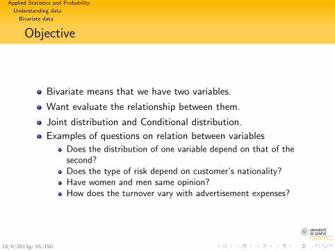
Bivariate means that we have two variables.
Want evaluate the relationship between them.
Joint distribution and Conditional distribution.
Examples of questions on relation between variables
Does the distribution of one variable depend on that of thesecond?Does the type of risk depend on customer’s nationality?Have women and men same opinion?How does the turnover vary with advertisement expenses?
18/9/2013gr 55/150
Applied Statistics and Probability
Understanding data
Bivariate data
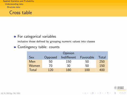
Cross table
For categorical variablesinclusive those defined by grouping numeric values into classes
Contingency table: counts
OpinionSex Opposed Indifferent Favorable TotalMen 50 150 50 250Women 70 30 50 150Total 120 180 100 400
18/9/2013gr 56/150
Applied Statistics and Probability
Understanding data
Bivariate data
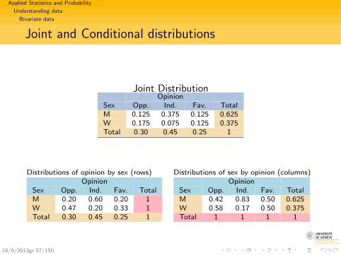
Joint and Conditional distributions
Joint DistributionOpinion
Sex Opp. Ind. Fav. TotalM 0.125 0.375 0.125 0.625W 0.175 0.075 0.125 0.375Total 0.30 0.45 0.25 1
Distributions of opinion by sex (rows)Opinion
Sex Opp. Ind. Fav. TotalM 0.20 0.60 0.20 1W 0.47 0.20 0.33 1Total 0.30 0.45 0.25 1
Distributions of sex by opinion (columns)Opinion
Sex Opp. Ind. Fav. TotalM 0.42 0.83 0.50 0.625W 0.58 0.17 0.50 0.375Total 1 1 1 1
18/9/2013gr 57/150
Applied Statistics and Probability
Understanding data
Bivariate data
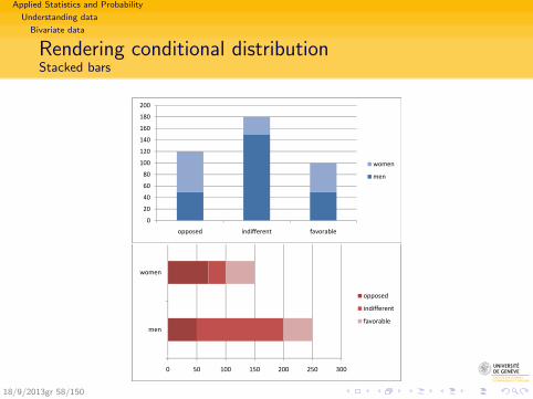
Rendering conditional distributionStacked bars
120
140
160
180
200
0
20
40
60
80
100
opposed indifferent favorable
women
men
womenwomen
opposed
men
indifferent
favorablemen
0 50 100 150 200 250 300
18/9/2013gr 58/150

Applied Statistics and Probability
Understanding data
Bivariate data
Numerical variables: Scatter plot
For numerical variables, a scatter plot informs on the natureof the relationship.
20.0
25.0
30.0
Return 2005
‐5.0
0.0
5.0
10.0
15.0
0 0
Return 200
5
‐10.0
0.0 5.0 10.0 15.0 20.0 25.0 30.0 35.0 40.0 45.0
3‐Year Return
18/9/2013gr 59/150
Applied Statistics and Probability
Understanding data
Bivariate data
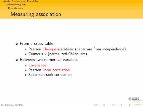
Measuring association
From a cross table
Pearson Chi-square statistic (departure from independence)Cramer’s v (normalized Chi-square)
Between two numerical variables
CovariancePearson linear correlationSpearman rank correlation
18/9/2013gr 60/150
Applied Statistics and Probability
Understanding data
Bivariate data
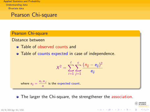
Pearson Chi-square
Pearson Chi-square
Distance between
Table of observed counts and
Table of counts expected in case of independence.
X 2 =∑i=1
c∑j=1
(nij − eij)2
eij
where eij =ni·n·j
nis the expected count.
The larger the Chi-square, the strengthener the association.
18/9/2013gr 61/150

Applied Statistics and Probability
Understanding data
Bivariate data
Cramer’s v
Chi-squares can only be compared for tables of same size andwith same grand total.
Practically, comparison with critical value function of ` and c.
Cramer’s v
Normalized form of Chi-square such that 0 ≤ v ≤ 1
v =
√X 2
n min{(`− 1), (c − 1)}
18/9/2013gr 62/150
Applied Statistics and Probability
Understanding data
Bivariate data
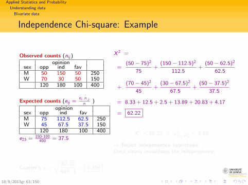
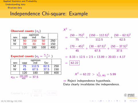
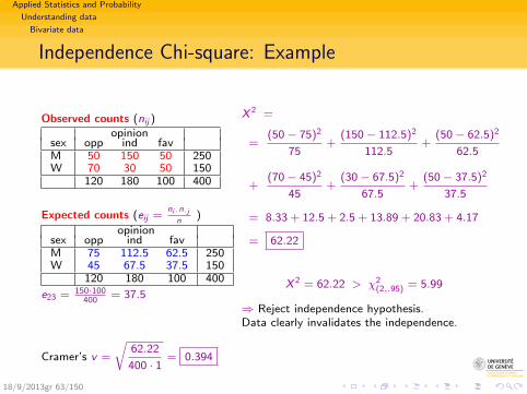
Independence Chi-square: Example
Observed counts (nij )opinion
sex opp ind favM 50 150 50 250W 70 30 50 150
120 180 100 400
Expected counts (eij =ni·n·j
n)
opinionsex opp ind favM 75 112.5 62.5 250W 45 67.5 37.5 150
120 180 100 400
e23 = 150·100400
= 37.5
X 2 =
=(50− 75)2
75+
(150− 112.5)2
112.5+
(50− 62.5)2
62.5
+(70− 45)2
45+
(30− 67.5)2
67.5+
(50− 37.5)2
37.5
= 8.33 + 12.5 + 2.5 + 13.89 + 20.83 + 4.17
= 62.22
X 2 = 62.22 > χ2(2,.95) = 5.99
⇒ Reject independence hypothesis.Data clearly invalidates the independence.
Cramer’s v =
√62.22
400 · 1= 0.394
18/9/2013gr 63/150
Applied Statistics and Probability
Understanding data
Bivariate data
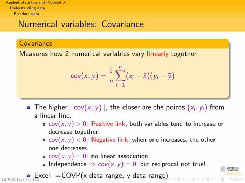
Numerical variables: Covariance
Covariance
Measures how 2 numerical variables vary linearly together
cov(x , y) =1
n
n∑i=1
(xi − x)(yi − y)
The higher | cov(x , y) |, the closer are the points (xi , yi ) froma linear line.
cov(x , y) > 0: Positive link, both variables tend to increase ordecrease together.cov(x , y) < 0: Negative link, when one increases, the otherone decreases.cov(x , y) = 0: no linear association.Independence ⇒ cov(x , y) = 0, but reciprocal not true!
Excel: =COVP(x data range, y data range)18/9/2013gr 64/150
Applied Statistics and Probability
Understanding data
Bivariate data
Pearson linear correlation
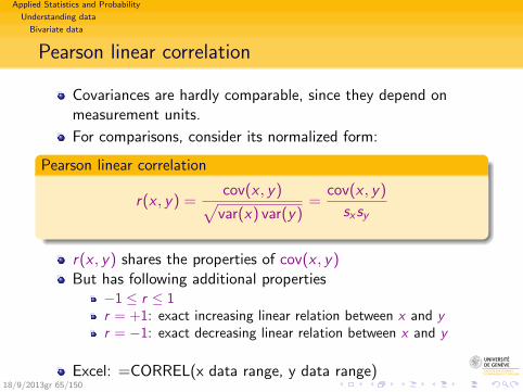
Covariances are hardly comparable, since they depend onmeasurement units.
For comparisons, consider its normalized form:
Pearson linear correlation
r(x , y) =cov(x , y)√
var(x) var(y)=
cov(x , y)
sxsy
r(x , y) shares the properties of cov(x , y)But has following additional properties
−1 ≤ r ≤ 1r = +1: exact increasing linear relation between x and yr = −1: exact decreasing linear relation between x and y
Excel: =CORREL(x data range, y data range)18/9/2013gr 65/150
Applied Statistics and Probability
Understanding data
Bivariate data
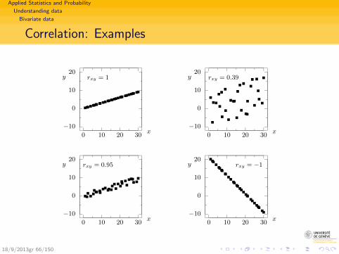
Correlation: Examples
0 10 20 30
20
10
0
−10
y
x
rxy = 1
0 10 20 30
20
10
0
−10
y
x
rxy = 0.39
0 10 20 30
20
10
0
−10
y
x
rxy = 0.95
0 10 20 30
20
10
0
−10
y
x
rxy = −1
18/9/2013gr 66/150
Applied Statistics and Probability
Understanding data
Linear Regression
Section outline
2 Understanding dataThe dataSoftwareExploratory univariate statistics
ObjectiveSummary tables and graphicsSummary numbers: central values, dispersion, ...Detecting and filtering out outliersModeling and comparing data distributions
Bivariate dataCross tabulationPlotting bivariate data: stacked bars, scatter plotMeasuring association
Linear RegressionMultiple Regression
Linearity in parameters and non linear relationsAbout non linear relations18/9/2013gr 67/150
Applied Statistics and Probability
Understanding data
Linear Regression
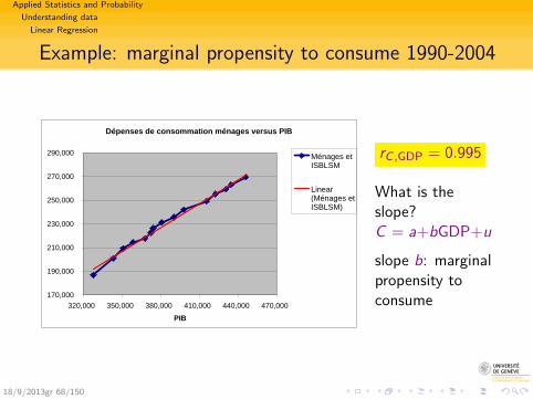
Example: marginal propensity to consume 1990-2004
Dépenses de consommation ménages versus PIB
170,000
190,000
210,000
230,000
250,000
270,000
290,000
320,000 350,000 380,000 410,000 440,000 470,000
PIB
Ménages etISBLSM
Linear(Ménages etISBLSM)
rC ,GDP = 0.995
What is theslope?C = a+bGDP+u
slope b: marginalpropensity toconsume
18/9/2013gr 68/150
Applied Statistics and Probability
Understanding data
Linear Regression
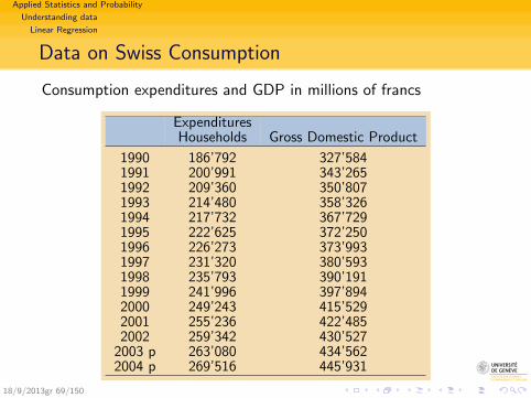
Data on Swiss Consumption
Consumption expenditures and GDP in millions of francs
ExpendituresHouseholds Gross Domestic Product
1990 186’792 327’5841991 200’991 343’2651992 209’360 350’8071993 214’480 358’3261994 217’732 367’7291995 222’625 372’2501996 226’273 373’9931997 231’320 380’5931998 235’793 390’1911999 241’996 397’8942000 249’243 415’5292001 255’236 422’4852002 259’342 430’527
2003 p 263’080 434’5622004 p 269’516 445’931
18/9/2013gr 69/150
Applied Statistics and Probability
Understanding data
Linear Regression
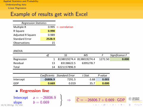
Example of results get with Excel
Regression StatisticsMultiple R 0.995 <‐ correlationR Square 0.990Adjusted R Square 0.989Standard Error 2528.9Observations 15
ANOVAdf SS MS F Significance F
Regression 1 8138019274.4 8138019274.4 1272.50 0.000Residual 13 83138622.5 6395278.7Total 14 8221157896.9
Coefficients Standard Error t Stat P‐valueIntercept ‐26806.9 7291.5 ‐3.68 0.003GDP 0.669 0.019 35.7 0.000
Regression line
Intercept a = −26806.9slope b = 0.669
}⇒ C = −26806.7 + 0.669 · GDP
18/9/2013gr 70/150

Applied Statistics and Probability
Understanding data
Linear Regression
Same regression in R
gdpc <- as.data.frame(read.table(file = paste(readir, "GDP-C-data.txt",
sep = ""), header = TRUE, sep = "\t"))
reg.simple <- lm(C ~ GDP, data = gdpc)
summary(reg.simple)
##
## Call:
## lm(formula = C ~ GDP, data = gdpc)
##
## Residuals:
## Min 1Q Median 3Q Max
## -5435 -1719 -445 1701 3649
##
## Coefficients:
## Estimate Std. Error t value Pr(>|t|)
## (Intercept) -26806.9060 7291.5049 -3.68 0.0028 **
## GDP 0.6686 0.0187 35.67 2.3e-14 ***
## ---
## Signif. codes: 0 '***' 0.001 '**' 0.01 '*' 0.05 '.' 0.1 ' ' 1
##
## Residual standard error: 2530 on 13 degrees of freedom
## Multiple R-squared: 0.99, Adjusted R-squared: 0.989
## F-statistic: 1.27e+03 on 1 and 13 DF, p-value: 2.35e-14
18/9/2013gr 71/150
Applied Statistics and Probability
Understanding data
Linear Regression
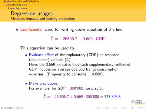
Regression usagesMeasures impacts and making predictions
Coefficients: Used for writing down equation of the line
C = −26806.7 + 0.669 · GDP
This equation can be used to
Evaluate effect of the explanatory (GDP) on response(dependent) variable (C).Here, the 0.669 indicates that each supplementary million ofGDP induces on average 669’000 francs consumptionexpenses. (Propensity to consume = 0.669).
Make predictions.For example, for GDP= 300′000, we predict
C = −26′806.7 + 0.669 · 300′000 = 173′893.3
18/9/2013gr 72/150
Applied Statistics and Probability
Understanding data
Linear Regression
Multiple regression
A regression is said multiple when there are more than oneexplanatory variables
Effect measured are controlled by the level of all othercovariates
Coefficient measure effect of the corresponding variableassuming all other variables remain unchanged.
18/9/2013gr 73/150
Applied Statistics and Probability
Understanding data
Linear Regression
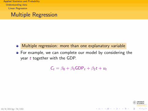
Multiple Regression
Multiple regression: more than one explanatory variable
For example, we can complete our model by considering theyear t together with the GDP.
Ct = β0 + β1GDPt + β2t + ut
18/9/2013gr 74/150
Applied Statistics and Probability
Understanding data
Linear Regression
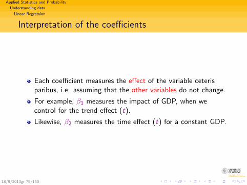
Interpretation of the coefficients
Each coefficient measures the effect of the variable ceterisparibus, i.e. assuming that the other variables do not change.
For example, β1 measures the impact of GDP, when wecontrol for the trend effect (t).
Likewise, β2 measures the time effect (t) for a constant GDP.
18/9/2013gr 75/150
Applied Statistics and Probability
Understanding data
Linear Regression
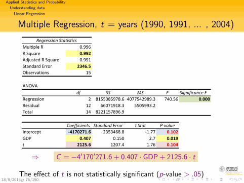
Multiple Regression, t = years (1990, 1991, ... , 2004)
Regression StatisticsMultiple R 0.996R Square 0.992Adjusted R Square 0.991Standard Error 2346.5Observations 15
ANOVAdf SS MS F Significance F
Regression 2 8155085978.6 4077542989.3 740.56 0.000Residual 12 66071918.3 5505993.2Total 14 8221157896.9
Coefficients Standard Error t Stat P‐valueIntercept ‐4170271.6 2353468.8 ‐1.77 0.102GDP 0.407 0.150 2.7 0.019t 2125.6 1207.4 1.76 0.104
⇒ C = −4′170′271.6 + 0.407 · GDP + 2125.6 · t
The effect of t is not statistically significant (p-value > .05)18/9/2013gr 76/150
Applied Statistics and Probability
Understanding data
Linear Regression
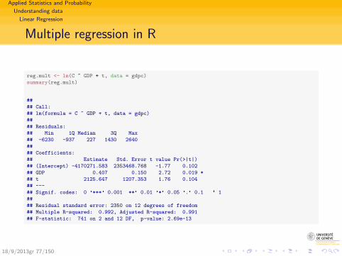
Multiple regression in R
reg.mult <- lm(C ~ GDP + t, data = gdpc)
summary(reg.mult)
##
## Call:
## lm(formula = C ~ GDP + t, data = gdpc)
##
## Residuals:
## Min 1Q Median 3Q Max
## -6230 -937 227 1430 2640
##
## Coefficients:
## Estimate Std. Error t value Pr(>|t|)
## (Intercept) -4170271.583 2353468.768 -1.77 0.102
## GDP 0.407 0.150 2.72 0.019 *
## t 2125.647 1207.353 1.76 0.104
## ---
## Signif. codes: 0 '***' 0.001 '**' 0.01 '*' 0.05 '.' 0.1 ' ' 1
##
## Residual standard error: 2350 on 12 degrees of freedom
## Multiple R-squared: 0.992, Adjusted R-squared: 0.991
## F-statistic: 741 on 2 and 12 DF, p-value: 2.69e-13
18/9/2013gr 77/150
Applied Statistics and Probability
Understanding data
Linearity in parameters and non linear relations
Section outline
2 Understanding dataThe dataSoftwareExploratory univariate statistics
ObjectiveSummary tables and graphicsSummary numbers: central values, dispersion, ...Detecting and filtering out outliersModeling and comparing data distributions
Bivariate dataCross tabulationPlotting bivariate data: stacked bars, scatter plotMeasuring association
Linear RegressionMultiple Regression
Linearity in parameters and non linear relationsAbout non linear relations18/9/2013gr 78/150
Applied Statistics and Probability
Understanding data
Linearity in parameters and non linear relations
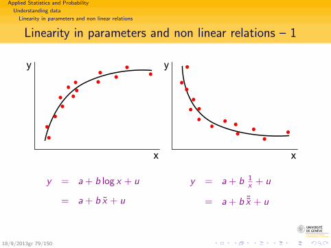
Linearity in parameters and non linear relations – 1
x
y
y = a + b log x + u
= a + b x + u
x
y
y = a + b 1x + u
= a + b ˜x + u
18/9/2013gr 79/150
Applied Statistics and Probability
Understanding data
Linearity in parameters and non linear relations
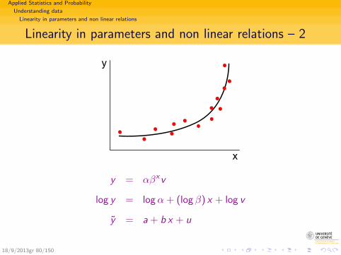
Linearity in parameters and non linear relations – 2
x
y
y = αβxv
log y = logα + (log β) x + log v
y = a + b x + u
18/9/2013gr 80/150
Applied Statistics and Probability
Understanding data
Linearity in parameters and non linear relations
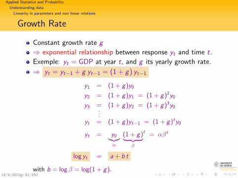
Growth Rate
Constant growth rate g
⇒ exponential relationship between response yt and time t.
Exemple: yt = GDP at year t, and g its yearly growth rate.
⇒ yt = yt−1 + g yt−1 = (1 + g) yt−1
y1 = (1 + g)y0
y2 = (1 + g)y1 = (1 + g)2y0
y3 = (1 + g)y2 = (1 + g)3y0...
yt = (1 + g)yt−1 = (1 + g)ty0
yt = y0︸︷︷︸α
(1 + g)︸ ︷︷ ︸β
t = αβt
log yt = a + b t
with b = log β = log(1 + g).18/9/2013gr 81/150
Applied Statistics and Probability
Understanding data
Linearity in parameters and non linear relations
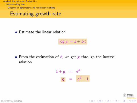
Estimating growth rate
Estimate the linear relation
log yt = a + b t
From the estimation of b, we get g through the inverserelation
1 + g = eb
g = eb − 1
18/9/2013gr 82/150
Applied Statistics and Probability
Inferential analysis
Outline
1 Introduction
2 Understanding data
3 Inferential analysis
4 Assessing regression results
18/9/2013gr 83/150
Applied Statistics and Probability
Inferential analysis
Sampling and probability
Section outline
3 Inferential analysisSampling and probability
Relationship between sample and populationBasic probability conceptsRandomness of sample mean and varianceExpected value and variance of sample statistics
Three main concepts for inferential purposesStandard errorMargin of errorStatistical significance
18/9/2013gr 84/150
Applied Statistics and Probability
Inferential analysis
Sampling and probability
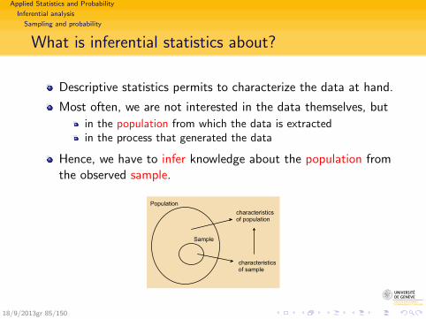
What is inferential statistics about?
Descriptive statistics permits to characterize the data at hand.
Most often, we are not interested in the data themselves, but
in the population from which the data is extractedin the process that generated the data
Hence, we have to infer knowledge about the population fromthe observed sample.
S a m p l e
P o p u l a t i o n
c h a r a c t e r i s t i c so f p o p u l a t i o n
c h a r a c t e r i s t i c so f s a m p l e
18/9/2013gr 85/150
Applied Statistics and Probability
Inferential analysis
Sampling and probability
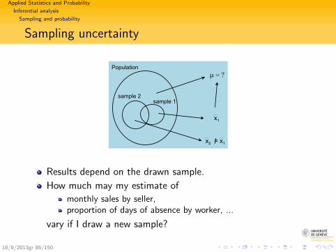
Sampling uncertainty
s a m p l e 1s a m p l e 2
P o p u l a t i o n
x 1
x 2 = x 1
m = ?
Results depend on the drawn sample.
How much may my estimate of
monthly sales by seller,proportion of days of absence by worker, ...
vary if I draw a new sample?
18/9/2013gr 86/150
Applied Statistics and Probability
Inferential analysis
Sampling and probability
Inferential statistics and probability
Inferential statistics is about evaluating
sampling uncertainty,confidence in the result.
Probability is natural way for that.
We first introduce basic concepts of probability
and then show how they apply in each of the two broadinferential approaches:
Estimation: evaluating value of quantitative characteristics.Statistical test: checking empirical support of an hypothesis.
18/9/2013gr 87/150
Applied Statistics and Probability
Inferential analysis
Sampling and probability
Probability
Probability
Numerical value representing the chance, likelihood orpossibility of a particular event A to occur.
0 ≤ prob(A) ≤ 1
A probability of 0 means no chance to occur.
A probability of 1 means event surely occurs.
Several approaches for determining probabilities:
Classical approachFrequency approach (also known as empirical approach)Subjective
18/9/2013gr 88/150
Applied Statistics and Probability
Inferential analysis
Sampling and probability
Event and Sample Space
A random process (e.g. randomly selecting a customer, a transaction, ...)
is a process with uncertain outcome.
Elementary outcome e: elementary outcome unit, generallythe selected case.
Sample space E : Collection of all elementary outcomes.
Event: Get a given characteristic
Set of elementary outcomes with the expected characteristics.e.g. customer ordering for more than ..., transaction on exactly3 items, ...
Special events
Impossible event: event realized for none of the elementaryoutcomes.Certain event: event realized for all elementary outcomes.
18/9/2013gr 89/150
Applied Statistics and Probability
Inferential analysis
Sampling and probability
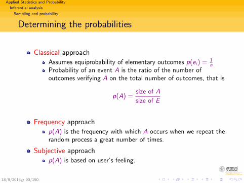
Determining the probabilities
Classical approach
Assumes equiprobability of elementary outcomes p(ei ) = 1n
Probability of an event A is the ratio of the number ofoutcomes verifying A on the total number of outcomes, that is
p(A) =size of A
size of E
Frequency approach
p(A) is the frequency with which A occurs when we repeat therandom process a great number of times.
Subjective approach
p(A) is based on user’s feeling.
18/9/2013gr 90/150
Applied Statistics and Probability
Inferential analysis
Sampling and probability
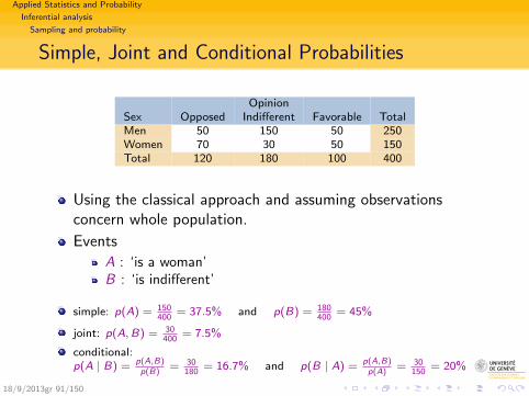
Simple, Joint and Conditional Probabilities
OpinionSex Opposed Indifferent Favorable TotalMen 50 150 50 250Women 70 30 50 150Total 120 180 100 400
Using the classical approach and assuming observationsconcern whole population.
Events
A : ‘is a woman’B : ‘is indifferent’
simple: p(A) = 150400
= 37.5% and p(B) = 180400
= 45%
joint: p(A,B) = 30400
= 7.5%
conditional:p(A | B) = p(A,B)
p(B)= 30
180= 16.7% and p(B | A) = p(A,B)
p(A)= 30
150= 20%
18/9/2013gr 91/150
Applied Statistics and Probability
Inferential analysis
Sampling and probability
Probability distribution
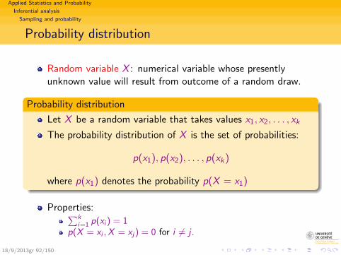
Random variable X : numerical variable whose presentlyunknown value will result from outcome of a random draw.
Probability distribution
Let X be a random variable that takes values x1, x2, . . . , xk
The probability distribution of X is the set of probabilities:
p(x1), p(x2), . . . , p(xk)
where p(x1) denotes the probability p(X = x1)
Properties:∑ki=1 p(xi ) = 1
p(X = xi ,X = xj) = 0 for i 6= j .
18/9/2013gr 92/150
Applied Statistics and Probability
Inferential analysis
Sampling and probability
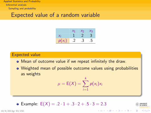
Expected value of a random variable
x1 x2 x3
xi 1 2 3p(xi ) .2 .3 .5
Expected value
Mean of outcome value if we repeat infinitely the draw.
Weighted mean of possible outcome values using probabilitiesas weights
µ = E(X ) =k∑
i=1
p(xi )xi
Example: E(X ) = .2 · 1 + .3 · 2 + .5 · 3 = 2.3
18/9/2013gr 93/150
Applied Statistics and Probability
Inferential analysis
Sampling and probability
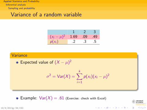
Variance of a random variable
1 2 3(xi − µ)2 1.69 .09 .49p(xi ) .2 .3 .5
Variance
Expected value of (X − µ)2
σ2 = Var(X ) =k∑
i=1
p(xi )(xi − µ)2
Example: Var(X ) = .61 (Exercise: check with Excel)
18/9/2013gr 94/150
Applied Statistics and Probability
Inferential analysis
Sampling and probability
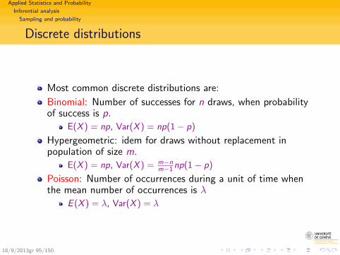
Discrete distributions
Most common discrete distributions are:
Binomial: Number of successes for n draws, when probabilityof success is p.
E(X ) = np, Var(X ) = np(1− p)
Hypergeometric: idem for draws without replacement inpopulation of size m.
E(X ) = np, Var(X ) = m−nm−1np(1− p)
Poisson: Number of occurrences during a unit of time whenthe mean number of occurrences is λ
E (X ) = λ, Var(X ) = λ
18/9/2013gr 95/150
Applied Statistics and Probability
Inferential analysis
Sampling and probability
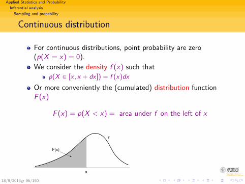
Continuous distribution
For continuous distributions, point probability are zero(p(X = x) = 0).
We consider the density f (x) such that
p(X ∈ [x , x + dx ]) = f (x)dx
Or more conveniently the (cumulated) distribution functionF (x)
F (x) = p(X < x) = area under f on the left of x
x
f
F ( x )
18/9/2013gr 96/150
Applied Statistics and Probability
Inferential analysis
Sampling and probability
Common continuous distributions
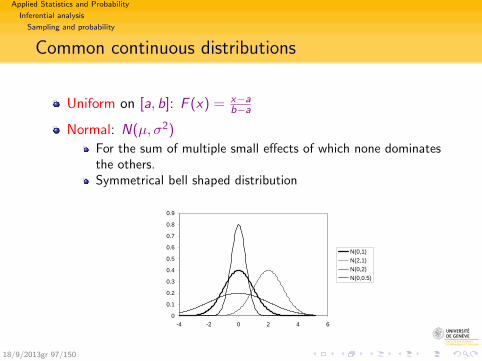
Uniform on [a, b]: F (x) = x−ab−a
Normal: N(µ, σ2)
For the sum of multiple small effects of which none dominatesthe others.Symmetrical bell shaped distribution
0
0.1
0.2
0.3
0.4
0.5
0.6
0.7
0.8
0.9
-4 -2 0 2 4 6
N(0,1)
N(2,1)
N(0,2)
N(0,0.5)
18/9/2013gr 97/150
Applied Statistics and Probability
Inferential analysis
Sampling and probability
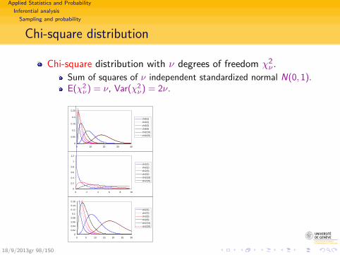
Chi-square distribution
Chi-square distribution with ν degrees of freedom χ2ν .
Sum of squares of ν independent standardized normal N(0, 1).E(χ2
ν) = ν, Var(χ2ν) = 2ν.
0
0.05
0.1
0.15
0.2
0.25
0 10 20 30 40
chi2(1)
chi2(2)
chi2(3)
chi2(5)
chi2(10)
chi2(20)
0
0.2
0.4
0.6
0.8
1
1.2
0 2 4 6 8 10
chi2(1)
chi2(2)
chi2(3)
chi2(5)
chi2(10)
chi2(20)
0
0.02
0.04
0.06
0.08
0.1
0.12
0.14
0.16
0 5 10 15 20 25 30
chi2(1)
chi2(2)
chi2(3)
chi2(5)
chi2(10)
chi2(20)
18/9/2013gr 98/150
Applied Statistics and Probability
Inferential analysis
Sampling and probability
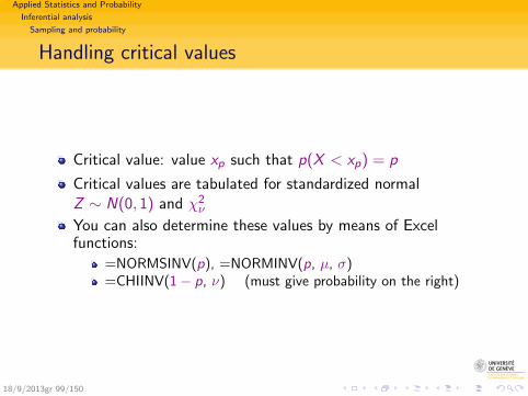
Handling critical values
Critical value: value xp such that p(X < xp) = p
Critical values are tabulated for standardized normalZ ∼ N(0, 1) and χ2
ν
You can also determine these values by means of Excelfunctions:
=NORMSINV(p), =NORMINV(p, µ, σ)=CHIINV(1− p, ν) (must give probability on the right)
18/9/2013gr 99/150
Applied Statistics and Probability
Inferential analysis
Sampling and probability
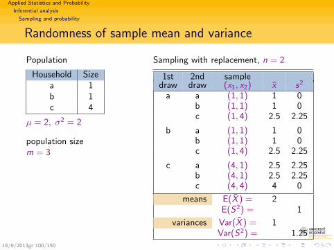
Randomness of sample mean and variance
Population
Household Sizea 1b 1c 4
µ = 2, σ2 = 2
population sizem = 3
Sampling with replacement, n = 2
1st 2nd sampledraw draw (x1, x2) x s2
a a (1, 1) 1 0b (1, 1) 1 0c (1, 4) 2.5 2.25
b a (1, 1) 1 0b (1, 1) 1 0c (1, 4) 2.5 2.25
c a (4, 1) 2.5 2.25b (4, 1) 2.5 2.25c (4, 4) 4 0
means E(X ) = 2E(S2) = 1
variances Var(X ) = 1Var(S2) = 1.25
18/9/2013gr 100/150

Applied Statistics and Probability
Inferential analysis
Sampling and probability
Distribution of sample mean and variance
x 1 2.5 4p(X = x) 4/9 4/9 1/9
E(X ) = 14
9+ 2.5
4
9+ 4
1
9= 2 = µ
Var(X ) = (−1)2 4
9+(1
2
)2 4
9+ 22 1
9= 1 =
σ2
n
s2 0 2.25p(S2 = s2) 5/9 4/9
E(S2) = 05
9+ 2.25
4
9= 1 =
n − 1
nσ2
Var(S2) = (−1)2 5
91 + (1.25)2 4
9= 1.25
18/9/2013gr 101/150
Applied Statistics and Probability
Inferential analysis
Sampling and probability
Distribution of sample statistics
In statistics, we are mainly concerned with
sample mean XSample variance S2
Previous computation is not applicable
There are mn possible samplesFor m = 10′000 and n = 100, we havemn = 10′000100 = 10400 samples
Luckily, we can use nice results about:
Expectation of sample statistics X , S2, ...Variance of sample statistics X , S2, ...
18/9/2013gr 102/150
Applied Statistics and Probability
Inferential analysis
Sampling and probability
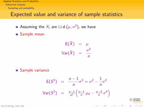
Expected value and variance of sample statistics
Assuming the Xi are i.i.d.(µ, σ2), we have
Sample mean
E(X ) = µ
Var(X ) =σ2
n
Sample variance
E(S2) =n − 1
nσ2 = σ2 − 1
nσ2
Var(S2) = n−1n2
(n−1n µ4 − n−3
n σ4)
18/9/2013gr 103/150
Applied Statistics and Probability
Inferential analysis
Sampling and probability
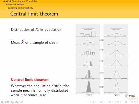
Central limit theorem
Distribution of Xi in population
Mean X of a sample of size n
Central limit theorem
Whatever the population distributionsample mean is normally distributedwhen n becomes large
0 1 2 3 4
0 1 2 3 4
0 1 2 3 4
0 1 2 3 4
0 1 2 3 4
0 1 2 3 4
0 1 2 3 4
0 1 2 3 4
0 1 2 3 4
0 1 2 3 4
0 1 2 3 4
0 1 2 3 4
n = 2
population quelconque
µ = 2.2
n = 3
n = 5
n = 10
n = 20
µ = 2.2
population normale
18/9/2013gr 104/150
Applied Statistics and Probability
Inferential analysis
Sampling and probability
Remark about sampling method
Previous results hold for independently and identicallydistributed (iid) Xi ’s.
Xi are iid for random sampling with replacementwithout repl. almost iid when sampling ratio n
m is low
Does not mean that this way of sampling is most efficient!
Following sampling methods are more efficient:
Sampling without replacementStratified samplingSampling by clusters
However, the simpler iid case is sufficient for understandingthe inferential principles.
18/9/2013gr 105/150
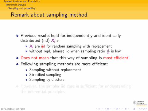
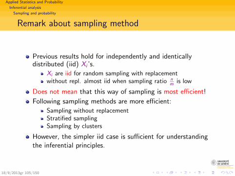
Applied Statistics and Probability
Inferential analysis
Three main concepts for inferential purposes
Section outline
3 Inferential analysisSampling and probability
Relationship between sample and populationBasic probability conceptsRandomness of sample mean and varianceExpected value and variance of sample statistics
Three main concepts for inferential purposesStandard errorMargin of errorStatistical significance
18/9/2013gr 106/150
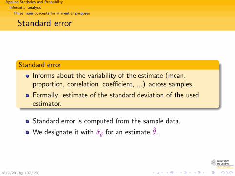
Applied Statistics and Probability
Inferential analysis
Three main concepts for inferential purposes
Standard error
Standard error
Informs about the variability of the estimate (mean,proportion, correlation, coefficient, ...) across samples.
Formally: estimate of the standard deviation of the usedestimator.
Standard error is computed from the sample data.
We designate it with σθ for an estimate θ.
18/9/2013gr 107/150
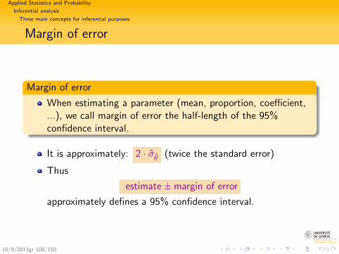
Applied Statistics and Probability
Inferential analysis
Three main concepts for inferential purposes
Margin of error
Margin of error
When estimating a parameter (mean, proportion, coefficient,...), we call margin of error the half-length of the 95%confidence interval.
It is approximately: 2 · σθ (twice the standard error)
Thus
estimate±margin of error
approximately defines a 95% confidence interval.
18/9/2013gr 108/150
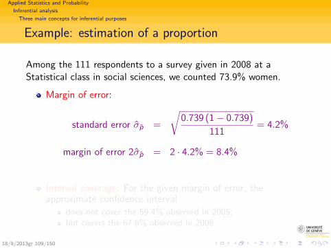
Applied Statistics and Probability
Inferential analysis
Three main concepts for inferential purposes
Example: estimation of a proportion
Among the 111 respondents to a survey given in 2008 at aStatistical class in social sciences, we counted 73.9% women.
Margin of error:
standard error σp =
√0.739 (1− 0.739)
111= 4.2%
margin of error 2σp = 2 · 4.2% = 8.4%
Interval coverage: For the given margin of error, theapproximate confidence interval
does not cover the 59.4% observed in 2005;but covers the 67.6% observed in 2006.
18/9/2013gr 109/150
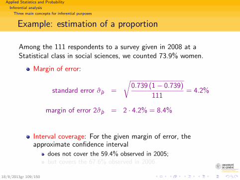
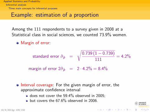
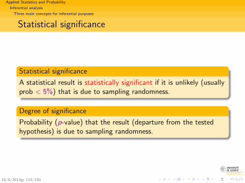
Applied Statistics and Probability
Inferential analysis
Three main concepts for inferential purposes
Statistical significance
Statistical significance
A statistical result is statistically significant if it is unlikely (usuallyprob < 5%) that is due to sampling randomness.
Degree of significance
Probability (p-value) that the result (departure from the testedhypothesis) is due to sampling randomness.
18/9/2013gr 110/150
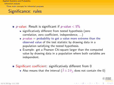
Applied Statistics and Probability
Inferential analysis
Three main concepts for inferential purposes
Significance: rules
p-value: Result is significant if p-value < 5%
significatively different from tested hypothesis (zerocorrelation, zero coefficient, independence, ...)p-value = probability to get a value more extreme than theobserved value of the test statistic by drawing data in apopulation satisfying the tested hypothesis.Example: get a Pearson Chi-square larger than the computedvalue by drawing data in a population where both variables areindependent.
Significant coefficient: significatively different from 0
Also means that the interval (β ± 2 σβ does not contain the 0)
18/9/2013gr 111/150
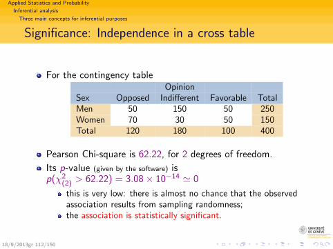
Applied Statistics and Probability
Inferential analysis
Three main concepts for inferential purposes
Significance: Independence in a cross table
For the contingency tableOpinion
Sex Opposed Indifferent Favorable TotalMen 50 150 50 250Women 70 30 50 150Total 120 180 100 400
Pearson Chi-square is 62.22, for 2 degrees of freedom.
Its p-value (given by the software) isp(χ2
(2) > 62.22) = 3.08× 10⁻¹⁴ ' 0
this is very low: there is almost no chance that the observedassociation results from sampling randomness;the association is statistically significant.
18/9/2013gr 112/150
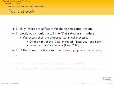
Applied Statistics and Probability
Inferential analysis
Three main concepts for inferential purposes
Put it at work
Luckily, there are software for doing the computation.
In Excel, you should install the ‘Data Analysis’ moduleYou access then the proposed statistical processes
On the right of the ‘Data’ menu tab (Excel 2007 and higher)From the ‘Data’ menu item (Excel 2003)
In R there are functions such as t.test, prop.test, chisq.test,
...
It is your task, however, to interpret the results.
So, let us go R (or Excel) and try it with some data sets ....
18/9/2013gr 113/150
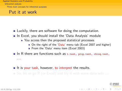
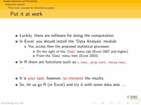
Applied Statistics and Probability
Assessing regression results
Outline
1 Introduction
2 Understanding data
3 Inferential analysis
4 Assessing regression results
18/9/2013gr 114/150
Applied Statistics and Probability
Assessing regression results
Assessing statistical relevance of a regression
Section outline
4 Assessing regression resultsAssessing statistical relevance of a regression
Reliability of parameter estimations
Global goodness of fitAnalysis of residualsMulticollinearity
18/9/2013gr 115/150
Applied Statistics and Probability
Assessing regression results
Assessing statistical relevance of a regression
Results from Excel
Regression StatisticsMultiple R 0.995 <‐ correlationR Square 0.990Adjusted R Square 0.989Standard Error 2528.9Observations 15
ANOVAdf SS MS F Significance F
Regression 1 8138019274.4 8138019274.4 1272.50 0.000Residual 13 83138622.5 6395278.7Total 14 8221157896.9
Coefficients Standard Error t Stat P‐valueIntercept ‐26806.9 7291.5 ‐3.68 0.003GDP 0.669 0.019 35.7 0.000
18/9/2013gr 116/150
Applied Statistics and Probability
Assessing regression results
Assessing statistical relevance of a regression
Same regression in R
reg.simple <- lm(C ~ GDP, data = gdpc)
summary(reg.simple)
##
## Call:
## lm(formula = C ~ GDP, data = gdpc)
##
## Residuals:
## Min 1Q Median 3Q Max
## -5435 -1719 -445 1701 3649
##
## Coefficients:
## Estimate Std. Error t value Pr(>|t|)
## (Intercept) -26806.9060 7291.5049 -3.68 0.0028 **
## GDP 0.6686 0.0187 35.67 2.3e-14 ***
## ---
## Signif. codes: 0 '***' 0.001 '**' 0.01 '*' 0.05 '.' 0.1 ' ' 1
##
## Residual standard error: 2530 on 13 degrees of freedom
## Multiple R-squared: 0.99, Adjusted R-squared: 0.989
## F-statistic: 1.27e+03 on 1 and 13 DF, p-value: 2.35e-14
18/9/2013gr 117/150
Applied Statistics and Probability
Assessing regression results
Assessing statistical relevance of a regression
Multiple regression in R
reg.mult <- lm(C ~ GDP + t, data = gdpc)
summary(reg.mult)
##
## Call:
## lm(formula = C ~ GDP + t, data = gdpc)
##
## Residuals:
## Min 1Q Median 3Q Max
## -6230 -937 227 1430 2640
##
## Coefficients:
## Estimate Std. Error t value Pr(>|t|)
## (Intercept) -4170271.583 2353468.768 -1.77 0.102
## GDP 0.407 0.150 2.72 0.019 *
## t 2125.647 1207.353 1.76 0.104
## ---
## Signif. codes: 0 '***' 0.001 '**' 0.01 '*' 0.05 '.' 0.1 ' ' 1
##
## Residual standard error: 2350 on 12 degrees of freedom
## Multiple R-squared: 0.992, Adjusted R-squared: 0.991
## F-statistic: 741 on 2 and 12 DF, p-value: 2.69e-13
18/9/2013gr 118/150
Applied Statistics and Probability
Assessing regression results
Assessing statistical relevance of a regression
Reliability of obtained coefficients
Standard error, t-stat, p-value.
Standard error: estimated standard deviation of coefficients(sampling variation)
t-stat: ratio of coefficient on standard errorApproximative rule:coefficient statistically significant if |t| > 2.
p-value: probability to get a value greater or equal to theobtained estimate with a sample randomly drawn from apopulation where the coefficient is null.
18/9/2013gr 119/150
Applied Statistics and Probability
Assessing regression results
Assessing statistical relevance of a regression
Statistical significance of the coefficients
Statistically significant coefficient ⇔ p-value< 0.05
In our case, both coefficients are statistically significant
The statistics |t| (3.68 and 35.7) are greater than 2.The p-values (.003 and .000)are clearly less than .05.
18/9/2013gr 120/150
Applied Statistics and Probability
Assessing regression results
Global goodness of fit
Section outline
4 Assessing regression resultsAssessing statistical relevance of a regression
Reliability of parameter estimations
Global goodness of fitAnalysis of residualsMulticollinearity
18/9/2013gr 121/150
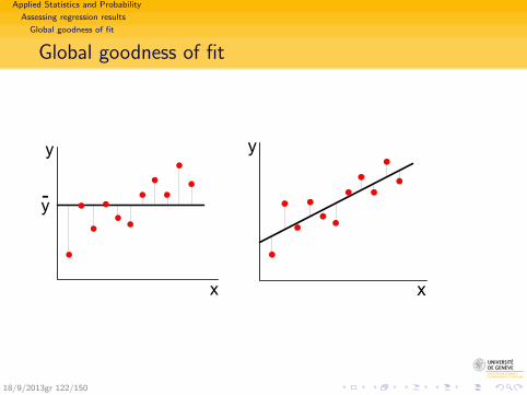
Applied Statistics and Probability
Assessing regression results
Global goodness of fit
Global goodness of fit
x
y
y -
x
y
18/9/2013gr 122/150
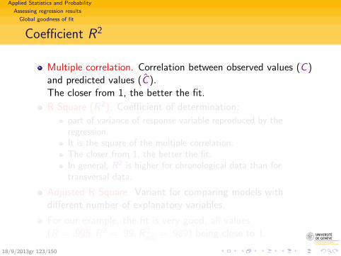
Applied Statistics and Probability
Assessing regression results
Global goodness of fit
Coefficient R2
Multiple correlation. Correlation between observed values (C )and predicted values (C ).The closer from 1, the better the fit.
R Square (R2). Coefficient of determination:
part of variance of response variable reproduced by theregression.It is the square of the multiple correlation.The closer from 1, the better the fit.In general, R2 is higher for chronological data than fortransversal data.
Adjusted R Square. Variant for comparing models withdifferent number of explanatory variables.
For our example, the fit is very good, all values(R = .995,R2 = .99,R2
adj = .989) being close to 1.
18/9/2013gr 123/150
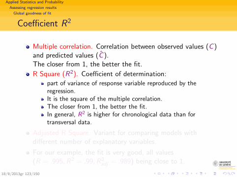
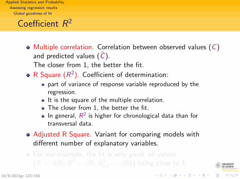
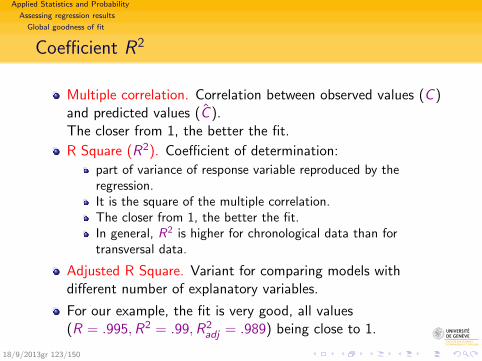
Applied Statistics and Probability
Assessing regression results
Global goodness of fit
Regression standard error
Regression standard error. Estimated standard deviation ofthe residuals (residual = difference between observed andpredicted values). Measures dispersion around the line.
It may be useful to compare this value with a measure of thedispersion of the response variable
18/9/2013gr 124/150
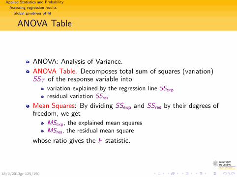
Applied Statistics and Probability
Assessing regression results
Global goodness of fit
ANOVA Table
ANOVA: Analysis of Variance.
ANOVA Table. Decomposes total sum of squares (variation)SST of the response variable into
variation explained by the regression line SSexp
residual variation SSres
Mean Squares: By dividing SSexp and SSres by their degrees offreedom, we get
MSexp, the explained mean squaresMSres, the residual mean square
whose ratio gives the F statistic.
18/9/2013gr 125/150
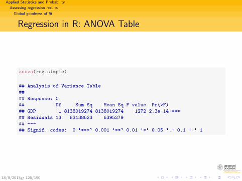
Applied Statistics and Probability
Assessing regression results
Global goodness of fit
Regression in R: ANOVA Table
anova(reg.simple)
## Analysis of Variance Table
##
## Response: C
## Df Sum Sq Mean Sq F value Pr(>F)
## GDP 1 8138019274 8138019274 1272 2.3e-14 ***
## Residuals 13 83138623 6395279
## ---
## Signif. codes: 0 '***' 0.001 '**' 0.01 '*' 0.05 '.' 0.1 ' ' 1
18/9/2013gr 126/150
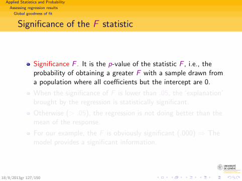
Applied Statistics and Probability
Assessing regression results
Global goodness of fit
Significance of the F statistic
Significance F . It is the p-value of the statistic F , i.e., theprobability of obtaining a greater F with a sample drawn froma population where all coefficients but the intercept are 0.
When the significance of F is lower than .05, the ‘explanation’brought by the regression is statistically significant.
Otherwise (> .05), the regression is not doing better than themean of the response.
For our example, the F is obviously significant (.000) ⇒ Themodel provides a significant information.
18/9/2013gr 127/150
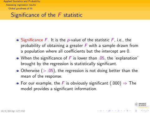
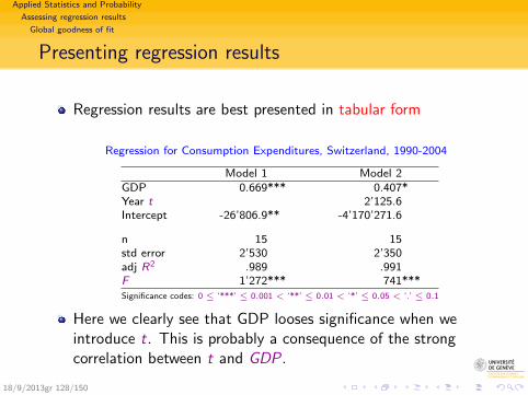
Applied Statistics and Probability
Assessing regression results
Global goodness of fit
Presenting regression results
Regression results are best presented in tabular form
Regression for Consumption Expenditures, Switzerland, 1990-2004
Model 1 Model 2GDP 0.669*** 0.407*Year t 2’125.6Intercept -26’806.9** -4’170’271.6
n 15 15std error 2’530 2’350adj R2 .989 .991F 1’272*** 741***Significance codes: 0 ≤ ‘***’ ≤ 0.001 < ‘**’ ≤ 0.01 < ‘*’ ≤ 0.05 < ‘.’ ≤ 0.1
Here we clearly see that GDP looses significance when weintroduce t. This is probably a consequence of the strongcorrelation between t and GDP.
18/9/2013gr 128/150
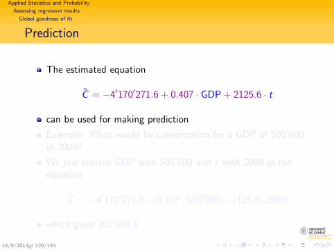
Applied Statistics and Probability
Assessing regression results
Global goodness of fit
Prediction
The estimated equation
C = −4′170′271.6 + 0.407 · GDP + 2125.6 · t
can be used for making prediction
Example: What would be consumption for a GDP of 500’000in 2009?
We just replace GDP with 500’000 and t with 2009 in theequation
C = −4′170′271.6 + 0.407 · 500′000 + 2125.6 · 2009
which gives 303′558.8
18/9/2013gr 129/150
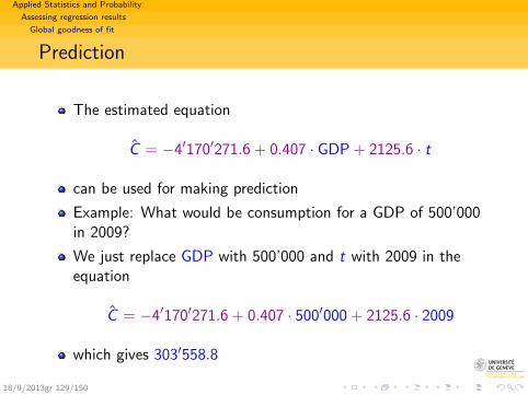
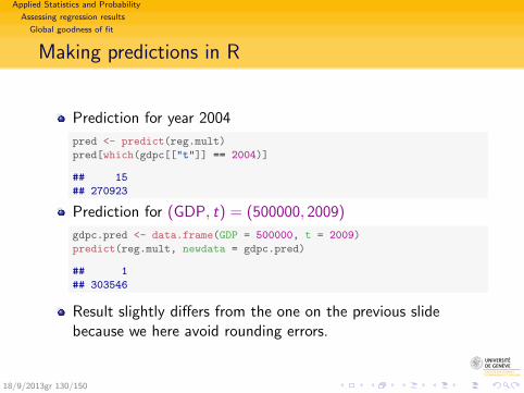
Applied Statistics and Probability
Assessing regression results
Global goodness of fit
Making predictions in R
Prediction for year 2004
pred <- predict(reg.mult)
pred[which(gdpc[["t"]] == 2004)]
## 15
## 270923
Prediction for (GDP, t) = (500000, 2009)
gdpc.pred <- data.frame(GDP = 500000, t = 2009)
predict(reg.mult, newdata = gdpc.pred)
## 1
## 303546
Result slightly differs from the one on the previous slidebecause we here avoid rounding errors.
18/9/2013gr 130/150
Applied Statistics and Probability
Assessing regression results
Analysis of residuals
Section outline
4 Assessing regression resultsAssessing statistical relevance of a regression
Reliability of parameter estimations
Global goodness of fitAnalysis of residualsMulticollinearity
18/9/2013gr 131/150
Applied Statistics and Probability
Assessing regression results
Analysis of residuals
Residuals
Regression model yi = β0 + β1x1i + · · ·+ βpxpi + ui
Predicted value: yi = β0 + β1x1i + · · ·+ βpxpi
Residual: for each observation, difference between actual andpredicted values
residual = actual− predicted
ri = yi − yi
18/9/2013gr 132/150
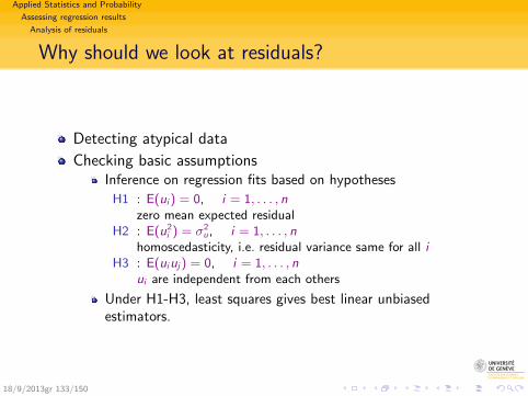
Applied Statistics and Probability
Assessing regression results
Analysis of residuals
Why should we look at residuals?
Detecting atypical data
Checking basic assumptionsInference on regression fits based on hypotheses
H1 : E(ui ) = 0, i = 1, . . . , nzero mean expected residual
H2 : E(u2i ) = σ2
u, i = 1, . . . , nhomoscedasticity, i.e. residual variance same for all i
H3 : E(uiuj) = 0, i = 1, . . . , nui are independent from each others
Under H1-H3, least squares gives best linear unbiasedestimators.
18/9/2013gr 133/150
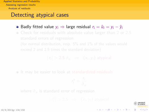
Applied Statistics and Probability
Assessing regression results
Analysis of residuals
Detecting atypical cases
Badly fitted value yi ⇒ large residual ri = ui = yi − yiCheck for residuals with absolute value larger than 2 or 2.5standard errors of regression.(for normal distribution, resp. 5% and 1% of the values would
exceed 2 and 2.5 times the standard deviation)
| ri | > 2.5 σu ⇒ (xi , yi ) atypical
It may be easier to look at standardized residuals
r si =riσu
where σu is standard error of regression
| r si | > 2.5 ⇒ (xi , yi ) atypical
18/9/2013gr 134/150
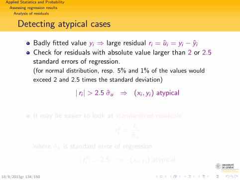
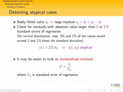
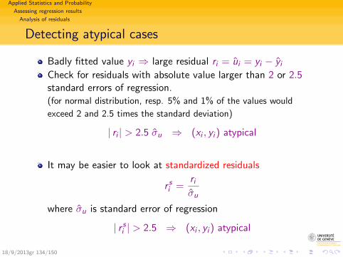
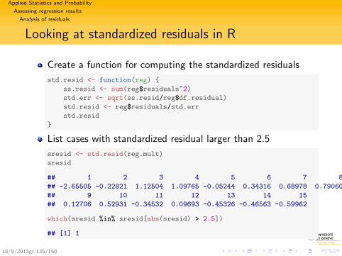
Applied Statistics and Probability
Assessing regression results
Analysis of residuals
Looking at standardized residuals in R
Create a function for computing the standardized residuals
std.resid <- function(reg) {
ss.resid <- sum(reg$residuals^2)
std.err <- sqrt(ss.resid/reg$df.residual)
std.resid <- reg$residuals/std.err
std.resid
}
List cases with standardized residual larger than 2.5
sresid <- std.resid(reg.mult)
sresid
## 1 2 3 4 5 6 7 8
## -2.65505 -0.22821 1.12504 1.09765 -0.05244 0.34316 0.68978 0.79060
## 9 10 11 12 13 14 15
## 0.12706 0.52931 -0.34532 0.09693 -0.45326 -0.46563 -0.59962
which(sresid %in% sresid[abs(sresid) > 2.5])
## [1] 1
18/9/2013gr 135/150
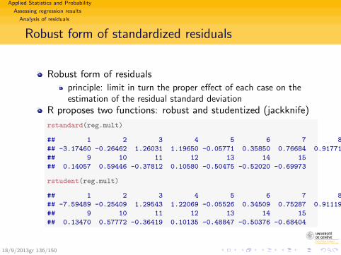
Applied Statistics and Probability
Assessing regression results
Analysis of residuals
Robust form of standardized residuals
Robust form of residuals
principle: limit in turn the proper effect of each case on theestimation of the residual standard deviation
R proposes two functions: robust and studentized (jackknife)
rstandard(reg.mult)
## 1 2 3 4 5 6 7 8
## -3.17460 -0.26462 1.26031 1.19650 -0.05771 0.35850 0.76684 0.91771
## 9 10 11 12 13 14 15
## 0.14057 0.59446 -0.37812 0.10580 -0.50475 -0.52020 -0.69973
rstudent(reg.mult)
## 1 2 3 4 5 6 7 8
## -7.59489 -0.25409 1.29543 1.22069 -0.05526 0.34509 0.75287 0.91119
## 9 10 11 12 13 14 15
## 0.13470 0.57772 -0.36419 0.10135 -0.48847 -0.50376 -0.68404
18/9/2013gr 136/150
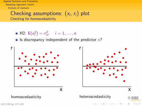
Applied Statistics and Probability
Assessing regression results
Analysis of residuals
Checking assumptions: (xi , ri) plotChecking for homoscedasticity
H2: E(u2i ) = σ2
u, i = 1, . . . , n
Is discrepancy independent of the predictor x?
x
r
homoscedasticity
x
r
heteroscedasticity
18/9/2013gr 137/150
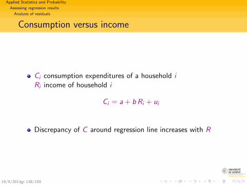
Applied Statistics and Probability
Assessing regression results
Analysis of residuals
Consumption versus income
Ci consumption expenditures of a household iRi income of household i
Ci = a + b Ri + ui
Discrepancy of C around regression line increases with R
18/9/2013gr 138/150
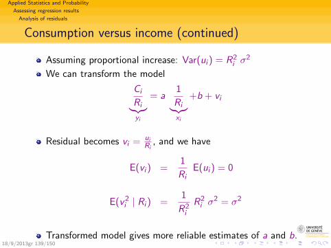
Applied Statistics and Probability
Assessing regression results
Analysis of residuals
Consumption versus income (continued)
Assuming proportional increase: Var(ui ) = R2i σ
2
We can transform the model
Ci
Ri︸︷︷︸yi
= a1
Ri︸︷︷︸xi
+b + vi
Residual becomes vi = uiRi
, and we have
E(vi ) =1
RiE(ui ) = 0
E(v2i | Ri ) =
1
R2i
R2i σ
2 = σ2
Transformed model gives more reliable estimates of a and b.18/9/2013gr 139/150
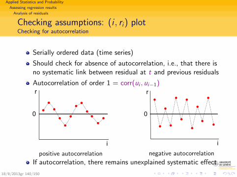
Applied Statistics and Probability
Assessing regression results
Analysis of residuals
Checking assumptions: (i , ri) plotChecking for autocorrelation
Serially ordered data (time series)
Should check for absence of autocorrelation, i.e., that there isno systematic link between residual at t and previous residuals
Autocorrelation of order 1 = corr(ui , ui−1)
i
r
0
positive autocorrelation
i
r
0
negative autocorrelation
If autocorrelation, there remains unexplained systematic effect.
18/9/2013gr 140/150
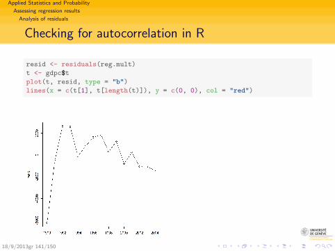
Applied Statistics and Probability
Assessing regression results
Analysis of residuals
Checking for autocorrelation in R
resid <- residuals(reg.mult)
t <- gdpc$t
plot(t, resid, type = "b")
lines(x = c(t[1], t[length(t)]), y = c(0, 0), col = "red")
18/9/2013gr 141/150
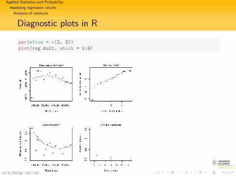
Applied Statistics and Probability
Assessing regression results
Analysis of residuals
Diagnostic plots in R
par(mfrow = c(2, 2))
plot(reg.mult, which = 1:4)
18/9/2013gr 142/150
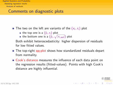
Applied Statistics and Probability
Assessing regression results
Analysis of residuals
Comments on diagnostic plots
The two on the left are variants of the (xi , ri ) plot
the top one is a (yi , ri ) plotthe bottom one is a (yi ,
√|ri,std |) plot
Both exhibit heteroscedasticity: higher dispersion of residualsfor low fitted values.
The top-right qq-plot shows how standardized residuals departfrom normality.
Cook’s distance measures the influence of each data point onthe regression results (fitted-values). Points with high Cook’sdistance are highly influential.
18/9/2013gr 143/150
Applied Statistics and Probability
Assessing regression results
Multicollinearity
Section outline
4 Assessing regression resultsAssessing statistical relevance of a regression
Reliability of parameter estimations
Global goodness of fitAnalysis of residualsMulticollinearity
18/9/2013gr 144/150
Applied Statistics and Probability
Assessing regression results
Multicollinearity
Multicollinearity
Multicollinearity
When one covariate is linear combination of the others,
Mathematically, when matrix X ′X is singular (determinant = 0)
Practically, we face a multicollinearity issue when a covariateis almost linearly dependent of the other ones (determinant of X ′X
very small)
In case of multicollinearity, the regression cannot distinguishthe effect of the variable from the effect of those it is linearlydependent.
Estimates of the coefficients become unstable.
18/9/2013gr 145/150
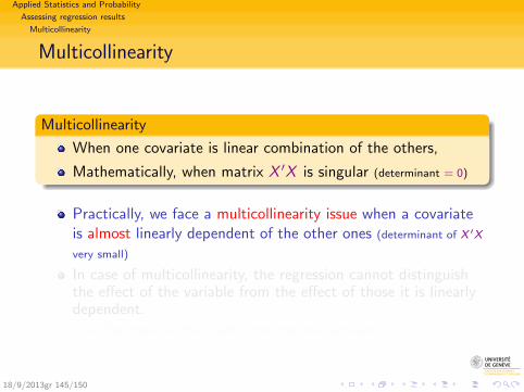
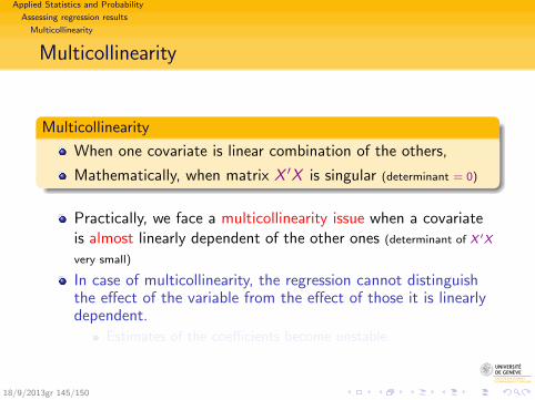

Applied Statistics and Probability
Assessing regression results
Multicollinearity
Multicollinearity diagnostics
In case of close multicollinearityGlobal fit remains good (not affected)
Involved coefficients become non significant, (because instable)
All coefficients nonsignificant + good fit (R2, F , Chi-square, ...)
are the sign of a collinearity issue.
VIF (Variance inflation factor): Measures by how much thevariance of the estimator of each coefficient increases when weintroduce the other variables.
VIF(βj) =1
1− R2j
where R2j is the R2 obtained by regressing xj on the other
covariates.Values of VIF exceeding 5 are considered evidence ofcollinearity.
18/9/2013gr 146/150
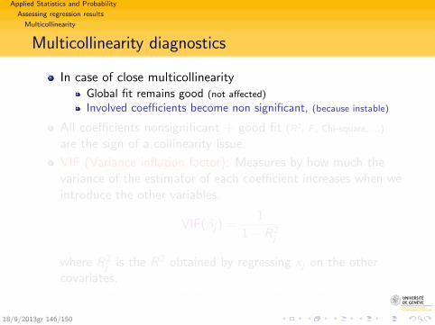
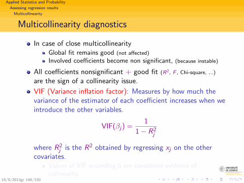
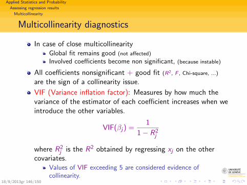
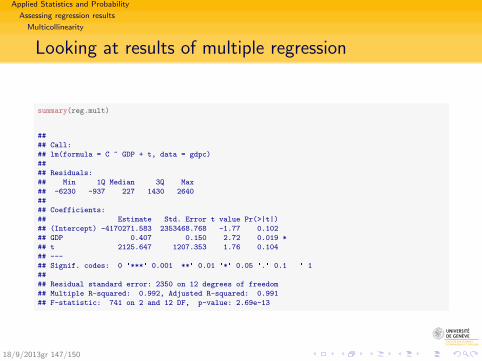
Applied Statistics and Probability
Assessing regression results
Multicollinearity
Looking at results of multiple regression
summary(reg.mult)
##
## Call:
## lm(formula = C ~ GDP + t, data = gdpc)
##
## Residuals:
## Min 1Q Median 3Q Max
## -6230 -937 227 1430 2640
##
## Coefficients:
## Estimate Std. Error t value Pr(>|t|)
## (Intercept) -4170271.583 2353468.768 -1.77 0.102
## GDP 0.407 0.150 2.72 0.019 *
## t 2125.647 1207.353 1.76 0.104
## ---
## Signif. codes: 0 '***' 0.001 '**' 0.01 '*' 0.05 '.' 0.1 ' ' 1
##
## Residual standard error: 2350 on 12 degrees of freedom
## Multiple R-squared: 0.992, Adjusted R-squared: 0.991
## F-statistic: 741 on 2 and 12 DF, p-value: 2.69e-13
18/9/2013gr 147/150

Applied Statistics and Probability
Assessing regression results
Multicollinearity
Example: VIF values
We have highly significant F and poorly significantcoefficients.
This is a sign of collinearityLet us check with the VIF values of the model
library(HH)
vif(reg.mult)
## GDP t
## 74.13 74.13
There is strong collinearity between GDP and t
18/9/2013gr 148/150
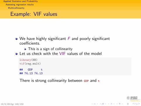
Applied Statistics and Probability
Assessing regression results
Multicollinearity
Complementing regression results
Useful to complement list of quality measures with
Maximum VIF value.Larger positive and negative standardized residuals.
18/9/2013gr 149/150

Applied Statistics and Probability
Assessing regression results
Multicollinearity
Bibliography I
Albright, S. C., W. Winston, and C. Zappe (2008). Data Analysis and DecisionMaking with Microsoft Excel (3rd Edition) (3rd ed.). South-Western CollegePublishing.
Levine, D. M., D. F. Stephan, T. C. Krehbiel, and M. L. Berenson (2008).Statistics for Managers: Using Microsoft Excel (5th ed.). Upper SaddleRiver, NJ, USA: Prentice Hall.
Maindonald, J. H. (2008). Using R for data analysis and graphics:Introduction, code and commentary. Manual, Centre for Mathematics andIts Applications, Austrialian National University.
R Development Core Team (2012). R: A Language and Environment forStatistical Computing. Vienna, Austria: R Foundation for StatisticalComputing. ISBN 3-900051-07-0.
Wonnacott, T. H. and R. J. Wonnacott (1990). Introductory statistics forbusiness and economics (Fourth ed.). New York: Wiley.
18/9/2013gr 150/150