Applied Mathematical Modelling 37 (2013) 384–397

Contents lists available at SciVerse ScienceDirect

Applied Mathematical Modelling

journal homepage: www.elsevier .com/locate /apm

Modeling and dynamic simulation of mixed feed multi-effect evaporatorsin paper industry

Deepak Kumar a,b,⇑, Vivek Kumar b, V.P. Singh b

a Department of Mathematics, Galgotias University, Greater Noida, UP, Indiab Department of Paper Technology, Indian Institute of Technology Roorkee, UK, India

a r t i c l e i n f o a b s t r a c t

Article history:Received 30 August 2010Received in revised form 16 February 2012Accepted 29 February 2012Available online 8 March 2012

Keywords:Multiple effect evaporatorMixed feedFsolveOde45Boiling point riseDynamic response

0307-904X/$ - see front matter � 2012 Elsevier Inchttp://dx.doi.org/10.1016/j.apm.2012.02.039

⇑ Corresponding author at: Department of MatheE-mail address: dkr2009@gmail.com (D. Kumar)

A wide range of mathematical models for multiple effect evaporators in process industryincluding paper industry are well reported in the literature but not so extensive work onthe dynamic behavior of MEE system is available in the literature. In the present studydynamic behavior of multi-effect evaporator system of a paper industry is obtained bydisturbing the feed flow rate, feed concentration, live steam temperature and feed temper-ature. For this purpose an unsteady-state model for the Multi-effect evaporator system isdeveloped. Each effect in the process is represented by a number of variables which arerelated by the energy and material balance equations for the feed, product and vapor flow.A generalized mathematical model which could be applied to any number of effects and allkinds of feeding arrangements like forward feed, backward feed, mixed feed and spilt feedin the MEE system with simple modifications was finally obtained. Finally model for mixedfeed sextuple effect falling film evaporators system was solved using MATLAB. For thesteady state and dynamic simulation the ‘fsolve’ and ‘ode45’ solvers in MATLAB sourcecode is used respectively.

� 2012 Elsevier Inc. All rights reserved.

1. Introduction

Pulp and paper industry is an energy intensive industry. Huge amount of raw material, chemical, energy and water areconsumed in the process of paper manufacturing. One such energy intensive subsystem, Multi-effect evaporator system(MEE), is used to concentrate black liquor from pulp mill. Rao and Kumar [1] indicated that the Multi-effect evaporatorsystem alone consumes around 24–30% of the total steam consumed in a large Indian paper mill.

The multiple effect evaporators (MEE) system in paper industry consists of a number of evaporators in series and largenumber of permutation and combinations are possible for feeding of black liquor and live steam. Dynamic behavior of suchsystem can only be studied by mathematical modeling and simulation.

A wide range of mathematical models for multiple effect evaporators in process industry including paper industry arewell reported in the literature. These mathematical modeling of MEE system are based on linear and non-linear mass andenergy balance equations, and relationships pertaining to the physical properties of the solution. These mathematical modelsare differentiated on the basis of the heuristic knowledge, which is incorporated in their development.

Various researchers have solved the mathematical models of MEE system of various process industries by using differentsolution techniques to obtain steady state simulation [2–19]. Some of them also have performed steady state simulation forMEE system of the paper industry [1,2,8–10,15,16,19,20] by solving the models using numerical techniques. The authors

. All rights reserved.

matics, Galgotias University, Greater Noida, UP, India. Tel.: +91 8126421115; fax: +91 132 2714311..

Nomenclature

A shell area, m2

BPR boiling point rise, �CC constantCp specific heat of water at constant pressure, kJ/kg KF feed, kg/sh enthalpy, kJ/kgL liquor level, mM mass, kgPl liquor densityt time, sT temperature, �CU overall heat transfer coefficient (OHTC), kW/m2 KW mass flow rate, kg/sX solid content, kg solids/kg totalk latent heat of vaporization

Subscriptsc condensatei effect numberl liquorv vapor

D. Kumar et al. / Applied Mathematical Modelling 37 (2013) 384–397 385

[1,2,8–10,20] have used Newton–Raphson method with Jacobian matrix and method of Gauss elimination with partial piv-oting supplemented with LU decomposition with the aid of Hilbert norms, and FORTRAN-77 language for computer pro-gramming. While the authors [15,16,19] simulated the MEE system using FORTRAN-90 and run the Pentium IV machine,using Microsoft FORTRAN power station 4.0 compiler.

Although the methods of design and steady state operation of single and multi-effect evaporators are well documented inthe literature but not so extensive work on the dynamic behavior of MEE system is available in the literature. The dynamicbehavior of two or three effect MEE systems in process industries like sugar, food, desalination and paper etc. is studied byfew researchers [12,21–26]. Miranda and Simpson [12] described a phenomenological, stationary and dynamic model of amultiple effect evaporator (tomato concentrate) for simulation and control purposes. Andre and Ritter [21] adequatelydescribed the open loop dynamic response of a laboratory scale double effect evaporator (for concentrating the sugar solu-tion) by a simple mathematical model based on the unsteady state material and energy balances associated with the variouselements of the system. Bolmstedt [22] developed a computer program for simulation of the dynamic behavior of generalmultiple effect evaporation plants. El-Nashar and Qamhiyeh [23] developed a simulation model for predicting the transientbehavior of Multi-effect stack-type (MES) distillation plant. Tonelli et al. [24] presented a computer package for the simula-tion of MEE for the concentration of liquid foods and studied the dynamic response. Narmine and Marwan [25] developed adynamic model for the MEE process to study the transient behavior of the system. Svandova et al. [26] has performed thesteady-state analysis and dynamic simulation of a methyl tertiary-butyl ether (MTBE) reactive distillation. Stefanov andHoo [27] developed a distributed parameter model of black liquor falling film evaporator, based on first principles knowl-edge and heat transfer processes for evaporation side of single plate (lamella) of a falling film evaporator. Stefanov andHoo [28] further expanded a single plate model to develop a fundamental model of a falling film evaporator that accountedfor the condensation side of the plate, the heating/flashing at the evaporator entrance, the evaporator inventory, mixing andrecirculation flows but neglecting the effect of BPR.

In the present investigation dynamic behavior of mixed feed six effect evaporators system is studied. For this purpose themathematical model of sextuple effect (tubular falling film with liquor flow inside the tube) falling film evaporator system ofa paper industry is developed based on the work reported by Narmine and Marwan [25]. Further the parametric equationswere solved for steady state conditions by vanishing the accumulation terms in model equations by using ‘fsolve’ solver inMATLAB source code. To study the transient behavior of the MEE system the solution of simultaneous ordinary differentialequations for sextuple mixed feed evaporator is obtained by using ‘ode45’ solver in MATLAB source code and the steady statesolution is used as the initial value.

2. Mathematical modelling

In the present investigation effect of BPR is also considered for and the mathematical modeling is developed for sextuplefalling film evaporator system with mixed feed based on the work proposed by Narmine and Marwan [25]. In the mixed feedsequence the feed is given to 5th effect and thick liquor coming out from 5th goes into 6th and from 6th to 4th and from 4th

Steam

Wv2=Wl3-Wl2 Wv3=Wl4-Wl3 Wv4=Wl6-Wl4 Wv5=F-Wl5 Wv6=Wl5-Wl6

Wl2 Wl3

Product

Condenser

c1 c2 c3 c4 c5 c6

Feed (F)

Wl4

Wl5

Wl6

Fig. 1. Flow diagram of sextuple mixed feed evaporator (? 5 ? 6 ? 4 ? 3 ? 2 ? 1).

Black liquor InletVapour

Outlet

ith Effect

Steam/Vapour Inlet Wli+1

Xi+1

Tli+1

Wvi

Tvi Wvi-1

Tvi-1

hvi-1

Wli

Xi

Tli

Steam Evaporation Chest Section

Wvi-1

hci-1

Fig. 2. Block diagram with terms used for the ith effect.

386 D. Kumar et al. / Applied Mathematical Modelling 37 (2013) 384–397

to 3rd and so on up to the first effect, while the steam input is given in the first effect as shown in the Fig. 1. The material andenergy flow for ith effect is given in the Fig. 2.

Model equations are developed for ith effect using material and energy balance equations. The equations stating the phys-ical properties of the black liquor are given in Table 1 defined by Gullichsen and Fogelholm [29]. It is assumed that the vaporgenerated by the process of concentration of black liquor is saturated. It is also assumed that the energy and mass accumu-lation in the vapor lump is very small as compared to the enthalpy of the steam and can be neglected.

Material balance for liquor in the ith effect for i = 1, 2 and 3:

Table 1Physico

S.no.

1.

2.

3.

4.5.

6.

ddt

MliðtÞ ¼Wliþ1 �Wli �Wvi: ð1Þ

Since in the mixed feed sequence the feed is given to fifth effect and then thick liquor move from 5th to 6th and from 6thto 4th effect thus for i = 4, 5 and 6 the equation is slightly different from the backward feed sequence and are given by

-thermal properties of black liquor, saturated steam and condensate.

Properties Equations Function parameters

Boiling point rise, �C BPR = (6.173X � 7.48X1.5 + 32.747X2) {1 + 0.006(Tv � 3.7316)} Solid concentration, (X); steamtemperature, (Tv) �C

Black liquor density, kg/m3 Pl = (997 + 649X) {1.008 – 0.237 (Tl/1000) – 1.94(Tl/1000)2} Black liquor temp. (Tl) in �C; solidconcentration, (X)

Specific heat capacity, kJ/kg K

Cp = 4.216(1 � X) + {1.675 + (3.31 Tl)/1000}X + (4.87 � 20 Tl/1000) (1 � X)X3

Black liquor temp. (Tl) in �C, solidconcentration, (X)

Enthalpy of water, kJ/kg hl = aT + b, where a = 4.1832 and b = 0.127011 Temp. of water, (T) in �CEnthalpy of saturatedsteam, kJ/kg

hv = c Tv + d, where c = 1.75228 and d = 2503.35 Steam temperature, (Tv) �C

Latent heat of vaporization,kJ/kg

k = 2519.5 � 2.653Tv Steam temperature, (Tv) �C

D. Kumar et al. / Applied Mathematical Modelling 37 (2013) 384–397 387

For i ¼ 4 the material balance equation isddt

Ml4ðtÞ ¼Wl6 �Wl4 �Wv4; ð1aÞ

Similarly for i ¼ 5 the material balance equation isddt

Ml5ðtÞ ¼ F�Wl5 �Wv5; ð1bÞ

In this way for i ¼ 6 the material balance equation isddt

Ml6ðtÞ ¼Wl5 �Wl6 �Wv6: ð1cÞ

Energy balance for liquor in the ith effect:

ddtðMliðtÞhliðtÞÞ ¼Wliþ1hliþ1 �Wlihli �Wvihvi þWvi�1hvi�1 �Wv i�1hci�1; ð2Þ

where Wvi�1 ¼ Qhvi�1�hci�1

and also Q ¼ UiAiðTviþ1 � Tv i � BPRiÞ.Material balance for solids in ith effect:

ddtðMliðtÞXiðtÞÞ ¼Wliþ1Xiþ1 �WliXi: ð3Þ

The changes shown in material balance for i = 4, 5 and 6 are similarly effective for energy and solid balance and in otherequations which are obtained by using material balances given by (1a), (1b) and (1c).

2.1. Formulation of the system equations

The modeling technique proposed by Narmine and Marwan [25] has been further modified and extended in the presentwork to obtain the mathematical modeling of the MEE system. The vapor and liquor in ith effect are in equilibrium and therelation for the liquor and vapor temperature defined in terms of BPR is as follows:

Tli ¼ Tvi þ BPRi ð4Þ

and the BPR is defined in terms of temperature and solid concentration, presented in Table 1.Differentiating Eq. (4) with respect to time we get

ddt

TliðtÞ ¼ddt

TviðtÞ� �

1þ o

oTvBPRi

� �� �þ o

oXBPRi

� �o

otXiðtÞ

� �: ð5Þ

Mli can be written as:

Mli ¼ ALiPli: ð6Þ

The Pli, the density of the liquor is defined in terms of temperature and solid concentration and also presented in Table 1.Differentiating Eq. (6) with respect to time we get

ddt

MliðtÞ ¼ ALiðtÞddt

Pli

� �þ APli

ddt

LiðtÞ� �

:

Since Pli is a function of temperature Tl and concentration X, this equation is reduces into Eq. (7) by using the value ofddt TliðtÞ from Eq. (5) with rearranging the terms.

ddt

MliðtÞ ¼ APliddt

LiðtÞ� �

þ ALiðtÞo

oTlPli

� �1þ o

oTvBPRi

� �ddt

TviðtÞ� �

þ ALiðtÞo

oTlPli

� �o

oXBPRi

� �þ o

oXPli

� �� �ddt

XiðtÞ� �

: ð7Þ

Comparing the resultant differential equation (7) with Eq. (1) we get

C1 ¼ C2ddt

LiðtÞ� �

þ C3ddt

TviðtÞ� �

þ C4ddt

XiðtÞ� �

; ð8Þ

where

C1 ¼Wliþ1 �Wli �Wvi;

C2 ¼ APli;

C3 ¼ ALiðtÞo

oTlPli

� �1þ o

oTvBPRi

� �� �;

Table 2Range of operational parameters.

S. no. Operational parameter Parameter’s range Target value

1 Liquor feed flow rate, kg/s 18.00–25.00 23.982 Liquor feed temperature, �C 70.00–90.00 80.003 Liquor feed concentration, kg solids/kg total 0.10–0.52 0.104 Steam temperature, �C 135–140 1395 Last body saturation, �C 48–52 496 Liquor product concentration, kg solids/kg total 0.48–0.52 0.507 Heat transfer coefficients (W/m2 K) 1160–1400 1160, 1220,1280, 1335, 1365, 1400

Table 3Steady

Item

InpuOutpInpuOutpInpuOutpInpuOutpInpuOutpBoiliSpec

HeatStreaTotaStea

388 D. Kumar et al. / Applied Mathematical Modelling 37 (2013) 384–397

C4 ¼ ALiðtÞo

oTlPli

� �o

oXBPRi

� �þ o

oXPli

� �� �:

Differentiating Mli(t)hli(t) with respect to time and using the value of ddt TliðtÞ from Eq. (5) and the value of d

dt MliðtÞ fromEq. (7) we get

ddt

MliðtÞ� �

hli þMliðtÞddt

hli

� �¼ APlihli

ddt

LiðtÞ� �

þ ALiðtÞ 1þ o

oTvBPRi

� �

Plio

oTlhli

� �þ o

oTlPli

� �hli

� �ddt

TviðtÞ� �

þ ALiðtÞddt

XiðtÞ� �

Plio

oTlhli

� �o

oXBPRi

� �þ Pli

o

oXhli

� �þ hli

o

oTlPli

� �o

oXBPRi

� �þ o

oXPli

� �hli

� �:

Comparing the resultant differential equation with Eq. (2) we get

C5 ¼ C6ddt

LiðtÞ� �

þ C7ddt

TviðtÞ� �

þ C8ddt

XiðtÞ� �

; ð9Þ

where

C5 ¼Wliþ1hliþ1 �Wlihli �Wvihvi þWvi�1hvi�1 �Wv i�1hci�1;

C6 ¼ APlihli;

C7 ¼ ALiðtÞð1þo

oTvBPRiÞ Pli

o

oTlhli

� �þ hli

o

oTlPli

� �� �;

C8 ¼ ALiðtÞPlio

oTlhli

� �o

oXBPEi

� �þ o

oXhli

� �� �þ ALiðtÞhli

o

oTlPli

� �o

oXBPRi

� �þ o

oXPli

� �� �:

Differentiating Mli(t)Xi(t) with respect to time and using the value of ddt MiðtÞ from Eq. (7) and rearranging the equation and

representing it in the form of coefficients

state solution of sextuple effect evaporator.

s Effects

I II III IV V VI

t liquor concentration (kg/kg) 0.2883 0.2067 0.1639 0.1401 0.1 0.1157ut liquor concentration (kg/kg) 0.5 0.2883 0.2067 0.1639 0.1157 0.1401t liquor flow (kg/s) 8.3173 11.6031 14.627 17.1105 23.98 20.73ut liquor flow (kg/s) 4.796 8.3173 11.6031 14.627 20.73 17.1105t liquor temperature (�C) 99.4662 83.4384 71.0077 50.419 80 61.3928ut liquor temperature (�C) 125.2157 99.4662 83.4384 71.0077 61.3928 50.419t steam temperature (�C) 139 111.0319 94.3051 80.5579 69.0649 60.2439ut steam temperature (�C) 111.0319 94.3051 80.5579 69.0649 60.2439 49t steam flow (kg/s) 3.8028 3.5213 3.2858 3.0239 2.4835 3.25ut steam flow (kg/s) 3.5213 3.2858 3.0239 2.4835 3.25 3.6195ng point rise (�C) 14.1838 5.1611 2.8805 1.9428 1.1489 1.419ific heat (kJ/kg K) 3.3006 3.6275 3.7704 3.8507 3.9506 3.8924

transfer area (m2) 591.9614m consumption (kg/s) 3.8028

l evaporation (kg/s) 19.184m economy 5.0447

0 1 2 3 4 5 648

50

52

54

56Variation in the Temperature of 6th effect with 10% decrease in feed flow rate

tx10-3 (s)

T (o C

)

0 1 2 3 4 5 642

44

46

48

50

T (o C

)

tx10-3 (s)

Variation in the Temperature of 6th effect with 10% increase in feed flow rate

0 0.2 0.4 0.6 0.8 1 1.2 1.4 1.6 1.8 20.140

0.141

0.142

0.143

0.144

tx10-4 (s)

X (k

g/kg

)

0.145

0 0.2 0.4 0.6 0.8 1 1.2 1.4 1.6 1.8 20.136

0.137

0.138

0.139

0.140

tx10-4 (s)

X (k

g/kg

)

0.141

Variation in the Product Concentration of 6th effect with 10% decrease in feed flow rate

Variation in the Product Concentration of 6th effect with 10% increase in feed flow rate

Fig. 3. Response of 6th effect by disturbing ±10% in the feed flow rate.

D. Kumar et al. / Applied Mathematical Modelling 37 (2013) 384–397 389

C9 ¼ C10ddt

LiðtÞ� �

þ C11ddt

TviðtÞ� �

þ C12ddt

XiðtÞ� �

; ð10Þ

where

C9 ¼Wliþ1Xiþ1 �WliXi;

C10 ¼ APliXi;

C11 ¼ ALiXio

oTlPli

� �1þ o

oTvBPRi

� �� �;

C12 ¼ ALi Pli þ Xio

oTlPli

� �o

oXBPRi

� �þ o

oXPli

� �� �� �:

0 1 2 3 4 5 6111

112

113

114

115

tx10-3 (s)

T (

o C)

Variation in the Temperature of 1st effect with 10% decrease in feed flow rate

0 0.5 1 1.5 2 2.5 3107

108

109

110

111

112

T (

o C)

0 1 2 3 4 5 6 7 8 90.50

0.52

0.54

0.56

X (

kg/k

g)

tx10-4 (s)

0 2 4 6 8 10 120.46

0.47

0.48

0.49

0.5

X (

kg/k

g)

tx10-4 (s)

Variation in the Product Concentration of 1st effect with 10% increase in feed flow rate

tx10-3 (s)

Variation in the Temperature of 1st effect with 10% increase in feed flow rate

Variation in the Product Concentration of 1st effect with 10% decrease in feed flow rate

Fig. 4. Response of first effect by disturbing ±10% in the feed flow rate.

390 D. Kumar et al. / Applied Mathematical Modelling 37 (2013) 384–397

3. Simulation

3.1. Steady state simulation

To study the dynamic response of any chemical process initial values of the process variables are needed, which can beobtained using steady state solution. For obtaining the steady state solution of the system, the accumulation terms in theEqs. (8)–(10) equal to zero i.e. C1 = 0, C5 = 0 and C9 = 0. Further substituting the values of physical properties like enthalpy,density, specific heat and boiling point rise from Table 1 and heat transfer rate from Eq. (2), mathematical model of 12 non-linear equations in 12 unknown variables is obtained. The model is similar to the model described by Ray and Sharma [10].

Operational data for simulation is taken from literature. For falling film evaporator the range of overall heat transfer coef-ficient (OHTC) is given by various researchers. Gupta [30] has suggested the value of OHTC as 580–2900 W/m2 K. Algehedand Berntsson [31] suggested the values of OHTC nearly 1510 W/m2 K. For evaporation of black liquor Gullichsen and Fogel-holm [29] suggested the range of OHTC for all six effects of a sextuple evaporator system between 500 and 2000 W/m2 K. Thevalues of OHTC depend on the concentration rise in the MEE system. After discussion with few Indian Paper Mills, values of

0 1 2 3 4 5 649

49.05

49.1

49.15

tx10-3 (s)

T (

o C)

Variation in the Temperature of 6th effect with 10% decrease in feed concentration

0 1 2 3 4 5 649

49.05

49.1

49.15

T (

o C)

Variation in the Temperature of 6th effect with 10% increase in feed concentration

tx10-3 (s)

0 1 2 3 4 5 60.125

0.13

0.135

0.14

0.145

tx10-4 (s)

X (

kg/k

g)

0 1 2 3 4 5 6

0.145

0.15

0.155

0.16

tx10-4 (s)

X (

kg/k

g)

Variation in the Product Concentration of 6th effect with 10% increase in feed concentration

0.140

Variation in the Product Concentration of 6th effect with 10% decrease in feed concentration

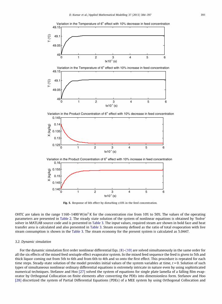
Fig. 5. Response of 6th effect by disturbing ±10% in the feed concentration.

D. Kumar et al. / Applied Mathematical Modelling 37 (2013) 384–397 391

OHTC are taken in the range 1160–1400 W/m2 K for the concentration rise from 10% to 50%. The values of the operatingparameters are presented in Table 2. The steady state solution of the system of nonlinear equations is obtained by ‘fsolve’solver in MATLAB source code and is presented in Table 3. The input values, required steam are shown in bold face and heattransfer area is calculated and also presented in Table 3. Steam economy defined as the ratio of total evaporation with livesteam consumption is shown in the Table 3. The steam economy for the present system is calculated as 5.0447.

3.2. Dynamic simulation

For the dynamic simulation first order nonlinear differential Eqs. (8)–(10) are solved simultaneously in the same order forall the six effects of the mixed feed sextuple effect evaporator system. In the mixed feed sequence the feed is given to 5th andthick liquor coming out from 5th to 6th and from 6th to 4th and so onto the first effect. This procedure is repeated for eachtime steps. Steady-state solution of the model provides initial values of the system variables at time, t = 0. Solution of suchtypes of simultaneous nonlinear ordinary differential equations is extremely intricate in nature even by using sophisticatednumerical techniques. Stefanov and Hoo [27] solved the system of equations for single plate lamella of a falling film evap-orator by Orthogonal Collocation on finite elements after converting the PDEs into dimensionless form. Stefanov and Hoo[28] discretized the system of Partial Differential Equations (PDEs) of a MEE system by using Orthogonal Collocation and

0 2 4 6 8 10 120.44

0.46

0.48

0.5

tx10-4 (s)

X (

kg/k

g)

0 1 2 3 4 5 6111

111.1

111.2

111.3

T (

o C)

Variation in the Temperature of 1st effect with 10% decrease in feed concentration

tx10-3 (s)

0 1 2 3 4 5 6111

111.1

111.2

111.3

T (

o C)

Variation in the Temperature of 1st effect with 10% increase in feed concentration

tx10-3 (s)

0 2 4 6 8 10 120.50

0.52

0.54

0.56

tx10-4 (s)

X (

kg/k

g)

Variation in the Product Concentration of 1st effect with 10% increase in feed concentration

Variation in the Product Concentration of 1st effect with 10% decrease in feed concentration

Fig. 6. Response of first effect by disturbing ±10% in the feed concentration.

392 D. Kumar et al. / Applied Mathematical Modelling 37 (2013) 384–397

then used LSODI (Livermore solver for ordinary differential equations, implicit system) solver, included in ODEPACK given byAlgehed and Berntsson [32] to solve the discretized system of PDEs. The execution time is approximately 14 h on a 1.2 GHzAthlon node, which is equivalent to 1 h of real time for dynamic simulation of plate type falling film MEE system for usingbackward feed. These techniques are complex and more time consuming. In the present investigation an attempt has beenmade for steady state as well as dynamic simulation for tubular type falling film MEE system for mixed feed by using ‘fsolve’and ‘ode45’ solver in MATLAB source code respectively. Simulations results obtained using MATLAB source code shows acomparable performance with FASTER method in terms of CPU time.

4. Model application

The dynamic response on system variables of MEE is studied by creating four types of disturbances namely (i) in feed flowrate, (ii) in feed concentration, (iii) in live steam temperature and (iv) in feed temperature as step input function. Systemvariables selected were (i) temperature of each effect and (ii) output concentration of each effect. The disturbance is taken

0 1 2 3 4 5 642

44

46

48

50

T (

o C)

tx10-3 (s)

Variation in the Temperature of 6th effect with 10% decrease in steam temperature

0 1 2 3 4 5 648

50

52

54

56

T (

o C)

tx10-3 (s)

Variation in the Temperature of 6th effect with 10% increase in steam temperature

0 1 2 3 4 5 60.1399

0.14

0.1401

0.1402

tx10-4 (s)

X (

kg/k

g)

0 1 2 3 4 5 60.14

0.1402

0.1404

0.1406

tx10-4 (s)

X (

kg/k

g)

Variation in the Product Concentration of 6th effect with 10% decrease in steam temperature

Variation in the Product Concentration of 6th effect with 10% increase in steam temperature

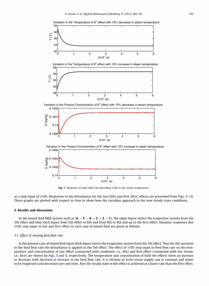
Fig. 7. Response of sixth effect by disturbing ±10% in the steam temperature.

D. Kumar et al. / Applied Mathematical Modelling 37 (2013) 384–397 393

as a step input of ±10%. Responses to the disturbance for the last (6th) and first (first) effects are presented from Figs. 3–10.These graphs are plotted with respect to time to show how the variables approach to the new steady state conditions.

5. Results and discussion

In the mixed feed MEE system such as (6 ? 5 ? 4 ? 3 ? 2 ? 1); the input liquor enters the evaporator system from the5th effect and then thick liquor from 5th effect to 6th and from 6th to 4th and up to the first effect. Dynamic responses due±10% step input in last and first effect in each case of mixed feed are given as follows.

5.1. Effect of varying feed flow rate

In the present case of mixed feed input thick liquor enters the evaporator system from the 5th effect. Thus for the variationin the feed flow rate the disturbance is applied in the 5th effect. The effect of ±10% step input in feed flow rate on the tem-perature and concentration of last effect (connected with condenser, i.e., 6th) and first effect (connected with live steam,i.e., first) are shown by Figs. 3 and 4, respectively. The temperature and concentration of both the effects show an increaseor decrease with decrease or increase in the feed flow rate. It is obvious as fresh steam supply rate is constant and waterto be evaporates and decreases per unit time. Also the steady state in 6th effect is achieved at a faster rate than the first effect.

0 1 2 3 4 5 6110

115

120

125

T (

o C)

tx10-3 (s)

0 1 2 3 4 5 6 7 8 9

0.496

0.498

0.5

0.502

tx10-4 (s)

X (

kg/k

g)

0.495

0 1 2 3 4 5 6 7 8 90.498

0.5

0.502

0.504

0.506

tx10-4 (s)

X (

kg/k

g)

0.5075

0 0.5 1 1.5 2 2.5 395

100

105

110

T (

o C)

tx10-3 (s)

Variation in the Temperature of 1st effect with 10% decrease in steam temperature

Variation in the Product Concentration of 1st effect with 10% increase in steam temperature

Variation in the Product Concentration of 1st effect with 10% decrease in steam temperature

Variation in the Temperature of 1st effect with 10% increase in steam temperature

Fig. 8. Response of first effect by disturbing ±10% in the steam temperature.

394 D. Kumar et al. / Applied Mathematical Modelling 37 (2013) 384–397

5.2. Effect of varying feed concentration

For the dynamic response of the feed concentration the disturbance is applied in the 5th effect. The effect of ±10% stepinput in feed concentration on the temperature and concentration of last (6th) and first effect (first) are shown in Figs. 5and 6, respectively. The dynamic behavior of effect’s temperature with respect to disturbances in feed concentration showsslight but insignificant change in temperature. However the change, it observed is unidirectional i.e. the temperature in-creases irrespective of increase or decrease in feed concentration. The changes in product concentration of both the effectshow increase or decrease according as the feed concentration is increase or decrease. This may be due to the fact thatDT across the evaporator system remains constant and vapor-liquid equilibrium of each effect remains almost unchangedfor the optimum performance.

5.3. Effect of varying steam temperature

In MEE system with mixed feed, live steam enters in the first effect. Thus for the variation in the steam temperature thedisturbance is applied in the first effect. The effect of ±10% step input in steam temperature on the temperature and concen-tration of last and first effect are shown in Figs. 7 and 8, respectively. The 10% change in steam temperature results in

0 1 2 3 4 5 6

48.6

48.8

49

49.2

T (

o C)

tx10-3 (s)

Variation in the Temperature of 6th effect with 10% decrease in feed temperature

48.4

0 1 2 3 4 5 649

49.2

49.4

49.6

49.8

T (

o C)

tx10-3 (s)

Variation in the Temperature of 6th effect with 10% increase in feed temperature

0 0.2 0.4 0.6 0.8 1 1.2 1.4 1.6 1.8 2

0.14015

0.1402

tx10-4 (s)

X (

kg/k

g)

Variation in the Product Concentration of 6th effect with 10% increase in feed temperature

0.1401

0 0.2 0.4 0.6 0.8 1 1.2 1.4 1.6 1.8 2

0.14015

0.1402

tx10-4 (s)

X (

kg/k

g)

Variation in the Product Concentration of 6th effect with 10% decrease in feed temperature

0.1401

Fig. 9. Response of sixth effect by disturbing ±10% in the feed temperature.

D. Kumar et al. / Applied Mathematical Modelling 37 (2013) 384–397 395

increase or decrease in the temperature of both the effects before obtaining the steady state for 10% increase or decreaserespectively. 10% disturbance in steam temperature does not result in any noticeable change in the product concentrationof both the effects. However with scale down Y-axis value (up to four decimal point as shown in the plots) it was observedthat product concentration increase and then decrease or decrease and then increase for 10% increase or decrease in thesteam temperature respectively.

5.4. Effect of varying feed temperature

Since feed liquor enters in the 5th effect for the mixed feed, thus the dynamic response of the feed temperature the dis-turbance is applied in the 5th effect. The effect of ±10% step change in feed temperature on the temperature and concentrationof last and first effect are shown by the Figs. 9 and 10, respectively. It is evident from the figures that 10% disturbance in feedtemperature does not bring noticeable change in the temperature and product concentration each effect. However with scaledown Y-axis (as shown in the plots), it is observed that temperature of the both the effect increases and decreases to obtain thesteady state with an increase and decrease in feed temperature and the product concentration of each effect first decreasesand then increases to obtain the steady state with a very small fluctuations about the steady state up to four to five decimal

0 1 2 3 4 5 6110.8

110.9

111

111.1

tx10-3 (s)

T (

o C)

0 1 2 3 4 5 6111

111.2

111.4

111.6

111.8

tx10-3 (s)

T (

o C)

Variation in the Temperature of 1st effect with 10% increase in feed temperature

0 2 4 6 8 10 120.4998

0.4999

0.5

0.5001

X (

kg/k

g)

Variation in the Product Concentration of 1st effect with 10% decrease in feed temperature

tx10-4 (s)

0 2 4 6 8 10 120.4999

0.5

0.5001

0.5002

X (

kg/k

g)

Variation in the Product Concentration of 1st effect with 10% increase in feed temperature

tx10-4 (s)

Variation in the Temperature of 1st effect with 10% decrease in feed temperature

Fig. 10. Response of first effect by disturbing ±10% in the feed temperature.

396 D. Kumar et al. / Applied Mathematical Modelling 37 (2013) 384–397

places in the value of concentrations of both the effect and conversely for 10% increase in feed temperature, which is negligiblein engineering problems.

6. Conclusions

For the steady state and dynamic simulation the ‘fsolve’ and ‘ODE45’ solvers in MATLAB source code are used successfully.Simulations results obtained using MATLAB source code show a comparable performance with faster method in terms of CPUtime and conclude that with the use of MATLAB it is possible to have better control of such complex system. Further thedynamic behavior of each effect’s temperature and product concentration was studied by disturbing the liquor flow rate,feed concentration, steam and feed temperatures by ±10%. The transient study shows that the steady state is reached morequickly for temperature in comparison of the solid concentration and all of the responses converge in a smooth fashion.

Acknowledgment

Mr. Deepak Kumar is thankful to Ministry of Human Resource Development; New Delhi, India for providing the SeniorResearch Fellowship for this work.

D. Kumar et al. / Applied Mathematical Modelling 37 (2013) 384–397 397

References

[1] N.J. Rao, R. Kumar, Energy conservation approaches in a paper mill with special reference to the evaporator plant, in: Proceedings of the IPPTAInternational Seminar Conservation in Pulp and, Paper Industry, 1985, pp. 58–70.

[2] A.K. Ray, N.J. Rao, M.C. Bansal, B. Mohanty, Design data and correlations of waste liquor/black liquor from pulp mills, IPPTA J. 4 (1992) 1–21.[3] W.T. Hanbury, Proc., IDA World Congress on Desalination and Water Sciences. Abu Dhabi, UAE, 4, 1995, p. 375.[4] H.T. El-Dessouky, I. Alatiqi, S. Bingulac, H.M. Ettouney, Steady-state analysis of the multiple effect evaporation desalination process, Chem. Eng.

Technol. 21 (5) (1998) 437–451.[5] H.T. El-Dessouky, H.M. Ettouney, F. Mandani, Performance of parallel feed multiple effect evaporation system for seawater desalination, Appl. Therm.

Eng. 20 (2000) 1679–1706.[6] H.T. El-Dessouky, H.M. Ettouney, F. Al-Juwayhel, Multiple effect evaporation-vapor compression desalination processes, Transactions of IChemE 78

(Part A) (2000) 662–676.[7] A.O.S. Costa, E.L. Enrique, Modeling of an industrial multiple effect evaporator system, in: Proceedings of the 35th Congresso e Exposicao Anual de

Celulose e Papel, 2002.[8] A.K. Ray, P. Singh, Simulation of multiple effect evaporator for black liquor concentration, IPPTA 12 (3) (2000) 35–45.[9] A.K. Ray, N.K. Sharma, P. Singh, Estimation of energy gains through modelling and simulation of multiple effect evaporator system in a paper mill,

IPPTA 16 (2) (2004) 35–45.[10] A.K. Ray, N.K. Sharma, Simulation of multi-effect evaporator for paper mill-effect of flash and product utilization for mixed feeds sequences, IPPTA 16

(4) (2004) 55–64.[11] V.K. Agarwal, M.S. Alam, S.C. Gupta, Mathematical model for existing multiple effect evaporator systems, Chemical Engineering World 39 (2004) 76–

78.[12] V. Miranda, R. Simpson, Modelling and simulation of an industrial multiple effect evaporator: tomato concentrate, J. Food Eng. 66 (2005) 203–210.[13] M. Karimi, A. Jahanmiri, M. Azarmi, Inferential cascade control of multi-effect falling-film evaporator, Food Control 18 (2007) 1036–1042.[14] D. Kaya, I.H. Sarac, Mathematical modeling of multiple-effect evaporators and energy economy, Energy 32 (2007) 1536–1542.[15] R. Bhargava, S. Khanam, B. Mohanty, A.K. Ray, Selection of optimal feed flow sequence for a multiple effect evaporator system, Computers and

Chemical Engineering 32 (2008) 2203–2216.[16] R. Bhargava, S. Khanam, B. Mohanty, A.K. Ray, Simulation of flat falling film evaporator system for concentration of black liquor, Computers and

Chemical Engineering 32 (2008) 3213–3223.[17] M.H. Khademi, M.R. Rahimpour, A. Jahanmiri, Simulation and optimization of a six-effect evaporator in a desalination process, Chem. Eng. Process. 48

(2009) 339–347.[18] M. Johansson, L. Vamling, L. Olausson, Heat transfer in evaporating black liquor falling film, Int. J. Heat Mass Transf. 52 (2009) 2759–2768.[19] S. Khanam, B. Mohanty, Energy reduction schemes for multiple effect evaporator systems, Appl. Energy 87 (2010) 1102–1111.[20] A. Gupta, Mathematical Modeling g and analysis of pulp washing problems, Ph.D. Thesis, Indian Institute of Technology Roorkee, 2001.[21] H. Andre, R.A. Ritter, Dynamic response of a double effect evaporator, Can. J. Chem. Eng. 46 (1968) 259–264.[22] U. Bolmstedt, Simulation of the steady-state and dynamic behavior of multiple effect evaporator plants, Part: 2 Dynamic Behavior, Comput. Aided Des.

9 (1) (1977) 29–40.[23] A.M. El-Nashar, A. Qamhiyeh, Simulation of the performance of MES evaporators under unsteady state operating conditions, Desalination 79 (1990)

65–83.[24] S. Tonelli, J.A. Romagnoli, J.A. Porras, Computer package for transient analysis of industrial multiple effect evaporators, J. Food Eng. 12 (1990) 267–281.[25] H.A. Narmine, M.A. Marwan, Dynamic response of multi-effect evaporators, Desalination 114 (1997) 189–196.[26] Z. Svandova, M. Kotora, J. Markos, L. Jelemensky, Dynamic behaviour of a CSTR with reactive distillation, Chem. Eng. J. 119 (2006) 113–120.[27] Z.I. Stefanov, K.A. Hoo, Distributed parameter model of black liquor falling-film evaporators. Part 1. Modeling of a single plate, Ind. Eng. Chem. Res. 42

(2003) 1925–1937.[28] Z.I. Stefanov, K.A. Hoo, Distributed parameter model of black liquor falling-film evaporators. 2. Modeling of a multiple-effect evaporator plant, Ind. Eng.

Chem. Res. 43 (2004) 8117–8132.[29] J. Gullichsen, C.J. Fogelholm, Chemical Pulping, Paper Making Science and Technology a series of 19 books, 6B, (2000), B18–20.[30] B.K. Dutta, Heat Transfer Principles and Applications, Prentice Hall of India Pvt. Ltd, New Delhi, 2005.[31] J. Algehed, T. Berntsson, Evaporation of black liquor and wastewater using medium-pressure steam: Simulation and economic evaluation of novel

designs, Appl. Therm. Eng. 23 (2003) 481–495.[32] A.C. Hindmarsh, ODEPACK a systemized collection of ODE solvers. Scientific Computing; 1 of IMACS Transactions on Scientific Computing; IMACS,

1982, 55–64.