Embed Size (px)
Citation preview

Outline Hodge Theory Applications Summary
Applied Hodge Theory
Yuan Yao
School of Mathematical SciencesPeking University
June 25th, 2014
Yuan Yao ICML’14: App. Hodge Theo.

Outline Hodge Theory Applications Summary
1 What’s Hodge TheoryHodge Theory on Riemannian ManifoldsHodge Theory on Metric SpacesCombinatorial Hodge Theory on Cell Complexes
2 Applications in Game Theory and Statistical RankingComputer VisionStatistical Ranking via Paired Comparison Method
HodgeRank on GraphsRandom Graph Models for SamplingRobust RankingOnline Algorithms
Game TheoryHodge Decomposition of Finite GamesBimatrix Games
3 Summary
Yuan Yao ICML’14: App. Hodge Theo.

Outline Hodge Theory Applications Summary
Topological & Geometric Methods in Data Analysis
Differential Geometric methods: manifolds• data distribution: manifold learning/NDR, etc.• model space: information geometry (high-order efficiency forparametric statistics)
Algebraic Geometric methods: polynomials/varieties• tensor (matrices etc.)• algebraic statistics• polynomial optimization (SOS)
Algebraic Topological methods: complexes (graphs, etc.)• persistent homology (robust, slow)• Euler calculus (non-stable, fast)• Hodge theory (geometry↔topology viaoptimization/spectrum)
Yuan Yao ICML’14: App. Hodge Theo.

Outline Hodge Theory Applications Summary
Helmholtz-Hodge Decomposition
Theorem (c.f. Marsden-Chorin 1992)
A vector field w on a simply-connected D can be uniquelydecomposed in the form
w = u + gradφ
where u has zero divergence and is parallel to ∂D.
Yuan Yao ICML’14: App. Hodge Theo.

Outline Hodge Theory Applications Summary
Algebraic Elements of Hodge Decomposition
For inner product spaces X , Y, and Z, consider
X A−→ Y B−→ Z.
and ∆ = AA∗ + B∗B : Y → Y where (·)∗ is adjoint operator of (·).If
B A = 0,
then ker(∆) = ker(A) ∩ ker(B∗) and orthogonal decomposition
Y = im(A) + ker(∆) + im(B∗)
Note: ker(B)/ im(A) ' ker(∆) is the (real) (co)-homology group(R→ rings; vector spaces→module).
Yuan Yao ICML’14: App. Hodge Theo.
Outline Hodge Theory Applications Summary
Hodge Theory on Riemannian Manifolds
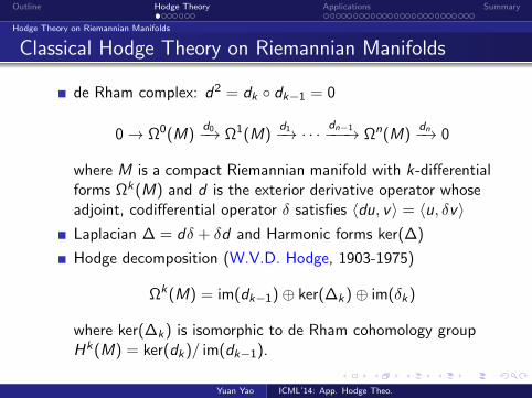
Classical Hodge Theory on Riemannian Manifolds
de Rham complex: d2 = dk dk−1 = 0
0→ Ω0(M)d0−→ Ω1(M)
d1−→ · · · dn−1−−−→ Ωn(M)dn−→ 0
where M is a compact Riemannian manifold with k-differentialforms Ωk(M) and d is the exterior derivative operator whoseadjoint, codifferential operator δ satisfies 〈du, v〉 = 〈u, δv〉Laplacian ∆ = dδ + δd and Harmonic forms ker(∆)
Hodge decomposition (W.V.D. Hodge, 1903-1975)
Ωk(M) = im(dk−1)⊕ ker(∆k)⊕ im(δk)
where ker(∆k) is isomorphic to de Rham cohomology groupHk(M) = ker(dk)/ im(dk−1).
Yuan Yao ICML’14: App. Hodge Theo.

Outline Hodge Theory Applications Summary
Hodge Theory on Metric Spaces
Hodge Theory on Metric Spaces
(Alexander-Spanier, Bartholdi-Schick-Smale-Smale, 2011)complex, d2 = 0
0→ L2(X )d0−→ L2(X 2)
d1−→ · · · dn−1−−−→ L2(X n)dn−→ ·
• L2(X ): square integral functions on metric space X• finite difference (Gilboa-Osher’08) d : L2(X k)→ L2(X k+1)
(df )(x0, . . . , xk) =k∑
i=1
(−1)i∏j 6=i
√K (xi , xj)f (x−i )
• adjoint operator δ : L2(X k+1)→ L2(X k)
δg(x) =k∑
i=0
(−1)i∫X
k−1∏j=0
√K (t, xj)g(x0, . . . , xi−1, t, xi , . . . , xk−1)dt
Yuan Yao ICML’14: App. Hodge Theo.

Outline Hodge Theory Applications Summary
Hodge Theory on Metric Spaces
continued: Hodge Theory on Metric Spaces
(Bartholdi-Schick-Smale-Smale-Baker, 2011)
If X satisfies some regularity conditions, then Hodgedecomposition holds
L2(X k) = im(dk−1)⊕ ker(∆k)⊕ im(δk)
In particular, if X is a compact Riemannian manifold withregularity conditions on convexity and curvature, there is ascale/kernel such that ker(∆k) is isomorphic to the L2-cohomologyand de Rham cohomology.
∆ = dδ + δdfor finite X , it essentially builds up a Cech complex for pointcloud data at certain scale and applies combinatorial Hodgetheory
Yuan Yao ICML’14: App. Hodge Theo.

Outline Hodge Theory Applications Summary
Combinatorial Hodge Theory on Cell Complexes
Combinatorial Hodge Theory on Cell Complexes
X is finite
χ(X ) ⊆ 2X is a simplicial complex formed by X , such thatτ ∈ χ(X ) and σ ⊆ τ , then σ ∈ χ(X )
k-forms or cochains as alternating functions
Ωk(X ) = u : χk+1(X )→ R, uiσ(0),...,iσ(k) = sign(σ)ui0,...,ik
where σ ∈ Sk+1 is a permutation on (0, . . . , k).
coboundary maps dk : Ωk(X )→ Ωk+1(X ) are defined as thealternating difference operator
(dku)(i0, . . . , ik+1) =k+1∑j=0
(−1)j+1u(i0, . . . , ij−1, ij+1, . . . , ik+1)
Yuan Yao ICML’14: App. Hodge Theo.

Outline Hodge Theory Applications Summary
Combinatorial Hodge Theory on Cell Complexes
Example: graph and clique complex
G = (X ,E ) is a undirected graph
Clique complex χG ⊆ 2X collects all complete subgraph of G
k-forms or cochains Ωk(χG ) as alternating functions:• 0-forms: v : V → R ∼= Rn
• 1-forms as skew-symmetric functions: wij = −wji
• 2-forms as triangular-curl:zijk = zjki = zkij = −zjik = −zikj = −zkji
coboundary operators dk : Ωk(χG )→ Ωk(χG ) as alternatingdifference operators:• (d0v)(i , j) = vj − vi =: (grad v)(i , j)• (d1w)(i , j , k) = (±)(wij + wjk + wki ) =: (curl w)(i , j , k)
d1 d0 = curl(grad u) = 0
Yuan Yao ICML’14: App. Hodge Theo.

Outline Hodge Theory Applications Summary
Combinatorial Hodge Theory on Cell Complexes
continued: Combinatorial Hodge Theory on Cell Complexes
So we have
0→ Ω0(X )d0−→ Ω1(X )
d1−→ · · · dn−1−−−→ Ωn(X )dn−→ · · ·
dk dk−1 = 0
combinatorial Laplacian ∆ = dk−1d∗k−1 + d∗kdk
• k = 0, ∆0 = d∗0d0 is the well-known graph Laplacian• k = 1, 1-Hodge Laplacian
∆1 = curl curl∗− div grad
Hodge decomposition holds for Ωk(X )• Ωk(X ) = im(dk−1)⊕ ker(∆k)⊕ im(δk)• dim(∆k) = βk(χ(X ))
Yuan Yao ICML’14: App. Hodge Theo.

Outline Hodge Theory Applications Summary
Combinatorial Hodge Theory on Cell Complexes
Forgetful functors
Riemannian manifolds→ Metric spaces→ Cell complexes
From differentiable to combinatorial structures, Hodgedecomposition is functorial (invariant)
Topological invariants (homology) are preserved in suchcoarse-grained functors
Natural for data analysis, a connection between geometry andtopology: harmonic basis
More important than data itself, relations between data viafunctions, mappings, etc.
Yuan Yao ICML’14: App. Hodge Theo.

Outline Hodge Theory Applications Summary
Applications of Hodge Decomposition
Boundary Value Problem (Schwarz, Chorin-Marsden’92)
Computer vision• Optical flow decomposition and regularization(Yuan-Schnorr-Steidl’2008, etc.)• Retinex theory and shade-removal(Ma-Morel-Osher-Chien’2011)• Relative attributes (Fu-Xiang-Y. et al. 2014)
Sensor Network coverage (Jadbabai et al.’10)
Statistical Ranking or Preference Aggregation(Jiang-Lim-Y.-Ye’2011, etc.)
Decomposition of Finite Games(Candogan-Menache-Ozdaglar-Parrilo’2011)
Yuan Yao ICML’14: App. Hodge Theo.

Outline Hodge Theory Applications Summary
Computer Vision
Optical Flow Decomposition and Regularization
Rudin-Osher-Fatemi’1992: piecewise constant flows
1
2‖v − u‖22 + TV (u), u, v ∈ R2
TV (u) :=
∫ √(grad u1)2 + (grad u2)2,
Yuan-Schnorr-Steidl’2007: piecewise harmonic flows
TV (u)→ R(u) =
∫ √(div u)2 + (curl u)2
Yuan Yao ICML’14: App. Hodge Theo.
Outline Hodge Theory Applications Summary
Computer Vision
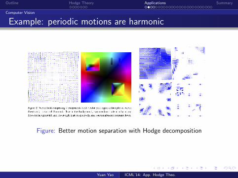
Example: periodic motions are harmonic
Figure: Better motion separation with Hodge decomposition
Yuan Yao ICML’14: App. Hodge Theo.

Outline Hodge Theory Applications Summary
Computer Vision
Adelson’s iIlusion in Computer Vision
Figure: Adelson’s illusion: on the left the chess board is shadowed by acolumn such that the white square has the same illuminance intensity asthe black square, proved by the right picture.
Yuan Yao ICML’14: App. Hodge Theo.

Outline Hodge Theory Applications Summary
Computer Vision
Retinex Theorey based on Approximation of Gradient Flows
The edge information is a gradient field of intensity grad I
Shade adds sparse noise Y = grad I + E
Find sparse approximation of de-noised gradient fieldminX ‖ grad X − T (Y )‖1
Figure: Ma-Morel-Osher-Chien 2011
Yuan Yao ICML’14: App. Hodge Theo.

Outline Hodge Theory Applications Summary
Statistical Ranking via Paired Comparison Method
Crowdsourcing QoE evaluation of Multimedia
Figure: (Xu-Huang-Y., et al. 11) Crowdsouring subjective Quality ofExperience evaluation
Yuan Yao ICML’14: App. Hodge Theo.

Outline Hodge Theory Applications Summary
Statistical Ranking via Paired Comparison Method
Learning relative attributes: age
2
2
3
1
2
Unintentional errorsIntentional errorsCorrect pairs
Ranking
scores:+10.6 -1.5
1
2
Figure: Age: a relative attribute estimated from paired comparisons(Fu-Y.-Xiang et al. 2013)
Yuan Yao ICML’14: App. Hodge Theo.

Outline Hodge Theory Applications Summary
Statistical Ranking via Paired Comparison Method
Collaborative Ideas Prioritization
10/18/13 CrowdRank | Your Ranking Engine with Real Consumer Reports - Consumers Report and Vote
www.crowdrank.net 1/3
Search
15.1 million votes cast
Insights Articles
Greatest AllTimeBasketball Player
Sexiest MAN Alive TV Brands Wireless Carriers
Sexiest Woman Alive Hotels MBA Best Dating Site
Colleges Airlines Beer Brewer Smartphone Brands
All Categories
CrowdRank
Read more
Last month, we shared an analysis of votes in our Sexiest Woman Alive category evaluating whether gentlemenprefer blondes. The overall answer was that globally men prefer brunettes but a slim 50.1% margin. But, theU.S. diverged from the global average and voters preferred blondes 50.9% of the time. The U.S. story gets moreinteresting, however, if we drill down to a state level. When we look at individual states, there is more parity: 21states show a preference for blondes, 18 prefer brunettes, and 7 prefer redheads. Meanwhile 4 states have noclear winner between blondes, brunettes, and redheads.
In the US, Do Gentlemen Prefer Blondes?
CrowdRank Insights
Brands Education Sports TV & Movies More
Nexus 7 from$229www.google.com/nexus
The 7" tablet fromGoogle with theworld's sharpestscreen. Buy now.
Flights fromChicago
The DepotRenaissanceMinneapolisHotelBeautifulChilean Girls
MBAMarketingDegree
Figure: Left: www.allourideas.org/wikipedia-banner-challenge, by Prof.Matt Salganik at Princeton; Right: www.crowdrank.net
Yuan Yao ICML’14: App. Hodge Theo.

Outline Hodge Theory Applications Summary
Statistical Ranking via Paired Comparison Method
Paired comparison data on graphs
Graph G = (V ,E )
V : alternatives to be ranked or rated
(iα, jα) ∈ E a pair of alternatives
yαij ∈ R degree of preference by rater α
ωαij ∈ R+ confidence weight of rater α
Examples: relative attributes, subjective QoE assessment,perception of illuminance intensity, sports, wine taste, etc.
Yuan Yao ICML’14: App. Hodge Theo.

Outline Hodge Theory Applications Summary
Statistical Ranking via Paired Comparison Method
Generalized Linear Models in Statistics: l2(E )
Majority voting (Condorcet’1785): inconsistency arises(Arrow’s impossibility theorem 1950s)
Statistical majority voting:• Yij = (
∑α ω
αij Y α
ij )/(∑
α ωαij ) = −Yji , ωij =
∑α ω
αij
Y from generalized linear models• Uniform model: Yij = 2πij − 1.
• Bradley-Terry model: Yij = logπij
1−πij .
• Thurstone-Mosteller model: Yij = Φ−1(πij).
Φ(x) =1√2π
∫ ∞−x/[2σ2(1−ρ)]1/2
e−12t2dt.
• Angular transform model: Yij = arcsin(2πij − 1).
Inner product induced on Y ∈ l2ω(E ), 〈u, v〉ω =∑
uijvijωij
where u, v skew-symmetric
Yuan Yao ICML’14: App. Hodge Theo.

Outline Hodge Theory Applications Summary
Statistical Ranking via Paired Comparison Method
Hodge Decomposition on Graphs [Jiang-Lim-Y.-Ye’11]
Paired comparison data Yij ∈ l2ω(E ) admits an orthogonaldecomposition,
Y = Y (g) + Y (h) + Y (c), (1)
whereY
(g)ij = βi − βj , for some θ ∈ RV , (2)
Y(h)ij + Y
(h)jk + Y
(h)ki = 0, for each i , j , k ∈ T , (3)∑
j∼iωij Y
(h)ij = 0, for each i ∈ V . (4)
Yuan Yao ICML’14: App. Hodge Theo.

Outline Hodge Theory Applications Summary
Statistical Ranking via Paired Comparison Method
Global ranking and Local vs. Global Inconsistencies
Y (g) = (δ0β)(i , j) := βi − βj where β solves
minβ∈R|V |
∑α,(i ,j)∈E
ωαij (βi − βj − Y αij )2 ⇔ ∆0β = δT0 Y
Residues Y (h) and Y (c) accounts for inconsistencies:
Y (c), the local inconsistency, triangular curls
• Y(c)ij + Y
(c)jk + Y
(c)ki 6= 0 , i , j , k ∈ T
Y (h), the global inconsistency, harmonic ranking• harmonic ranking leads to circular coordinates (MVJtutorial) on V ⇒ fixed tournament issue
Yuan Yao ICML’14: App. Hodge Theo.

Outline Hodge Theory Applications Summary
Statistical Ranking via Paired Comparison Method
Topological Constraints
To get a faithful ranking, two topological conditions on the cliquecomplex χ2
G = (V ,E ,T ) are important:
Connectivity: G is connected, then an unique global ranking ispossible;
Loop-free: harmonic ranking vanishes if χ2G is loop-free,
topology plays a role of obstruction of fixed-tournament• “Triangular arbitrage-free implies arbitrage-free”
Yuan Yao ICML’14: App. Hodge Theo.

Outline Hodge Theory Applications Summary
Statistical Ranking via Paired Comparison Method
Basic Problems in HodgeRank
sampling method for crowdsourcing• passive, active, random graph theory, etc.
reliability of data: inconsistency• outlier detection and robust ranking
sequential or streaming data: online algorithms• persistent homology, online ranking
Yuan Yao ICML’14: App. Hodge Theo.

Outline Hodge Theory Applications Summary
Statistical Ranking via Paired Comparison Method
Random Graph Models for Crowdsourcing
Recall that in crowdsourcing ranking on internet,• unspecified raters compare item pairs randomly• online, or sequentially sampling
random graph models for experimental designs• P a distribution on random graphs, invariant underpermutations (relabeling)• Generalized de Finetti’s Theorem [Aldous 1983, Kallenberg2005]: P(i , j) (P ergodic) is an uniform mixture of
h(u, v) = h(v , u) : [0, 1]2 → [0, 1],
h unique up to sets of zero-measure• Erdos-Renyi: P(i , j) = P(edge) =
∫ 10
∫ 10 h(u, v)dudv =: p
• edge-independent process (Chung-Lu’06)
Yuan Yao ICML’14: App. Hodge Theo.

Outline Hodge Theory Applications Summary
Statistical Ranking via Paired Comparison Method
Phase Transitions of Large Random Graphs
For an Erdos-Renyi random graph G (n, p) with n vertices and eachedge independently emerging with probability p(n),
(Erdos-Renyi 1959) One phase-transition for β0• p << 1/n1+ε (∀ε > 0), almost always disconnected• p >> log(n)/n, almost always connected
(Kahle 2009) Two phase-transitions for βk (k ≥ 1)• p << n−1/k or p >> n−1/(k+1), almost always βk vanishes;• n−1/k << p << n−1/(k+1), almost always βk is nontrivial
For example: with n = 16, 75% distinct edges included in G , thenχG with high probability is connected and loop-free. In general,O(n log(n)) samples for connectivity and O(n3/2) for loop-free.
Yuan Yao ICML’14: App. Hodge Theo.

Outline Hodge Theory Applications Summary
Statistical Ranking via Paired Comparison Method
Other sampling models
Random k-regular graphs• Kim-Vu sandwich theorem/conjecture: coupling withErdos-Renyi if edges are dense enough
Preferential-attachment random graphs• online but dependent (active) sampling• coupling with edge-independent process (Chung-Lu’06)
Geometric random graphs• ranking items from Euclidean feature space
Active sampling?• Osting, Brune, and Osher, ICML 2013• Osting, Xiong, Xu, and Y., 2014
Yuan Yao ICML’14: App. Hodge Theo.
Outline Hodge Theory Applications Summary
Statistical Ranking via Paired Comparison Method
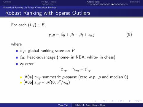
Robust Ranking with Sparse Outliers
For each (i , j) ∈ E ,
yαij = β0 + βi − βj + zαij (5)
where
βV : global ranking score on V
β0: head-advantage (home- in NBA, white- in chess)
zij errorzαij = γαij + εαij
• [A0a] γαij symmetric p-sparse (zero w.p. p and median 0)• [A0b] εαij ∼ N (0, σ2/wij)
Yuan Yao ICML’14: App. Hodge Theo.

Outline Hodge Theory Applications Summary
Statistical Ranking via Paired Comparison Method
Huber’s LASSO [Xiong-Cheng-Y.’13,Xu-Xiong-Huang-Y.’13]
Robust ranking can be formulated as a Huber’s LASSOproblem (Gannaz’07, She-Owen’09, Fan-Tang-Shi’12)
Sparse outliers are sparse approximation of cyclic rankings(curl+harmonic)
Exact recovery is possible without Gaussian noise
Outlier detection is possible against Gaussian noise, provided• Irrepresentable condition (e.g. random graph)• Outliers have large enough magnitudes
Yuan Yao ICML’14: App. Hodge Theo.

Outline Hodge Theory Applications Summary
Statistical Ranking via Paired Comparison Method
Exact Recover against pure Sparse Outliers
Theorem (Xiong-Cheng-Y.’2013)
Let G (n, q) be an Erdos-Renyi Random Graph with n nodes andeach edge drawn independently with probability q ∈ (0, 1].(A) Suppose that paired comparison data y is collected on G (n, q)subject to the linear model with symmetric p-sparse outliers(p ∈ [0, 1]). Then with probability tending to one the L1 solutionexactly recovers the global ranking β∗ if
p O
(√log n
nq
).
Note: no method can recover if
p O
(1√nq
).
Yuan Yao ICML’14: App. Hodge Theo.

Outline Hodge Theory Applications Summary
Statistical Ranking via Paired Comparison Method
Persistent Homology: online algorithm for topologytracking (e.g Edelsbrunner-Harer’08)
Figure: Persistent Homology Barcodes
vertice, edges, andtriangles etc.sequentially added
online update ofhomology
O(m) for surfaceembeddable complex;and O(m2.xx) ingeneral (m number ofsimplex)
Yuan Yao ICML’14: App. Hodge Theo.

Outline Hodge Theory Applications Summary
Statistical Ranking via Paired Comparison Method
Online HodgeRank as Stochastic Approximations
Robbins-Monro (1951) algorithm for Ax = b
xt+1 = xt − γt(Atxt − bt), E(At) = A, E(bt) = b
Now consider ∆0s = δ∗0Y , with new rating Yt(it+1, jt+1)
st+1(it+1) = st(it+1)− γt [st(it+1)− st(jt+1)− Yt(it+1, jt+1)]
st+1(jt+1) = st(jt+1) + γt [st(it+1)− st(jt+1)− Yt(it+1, jt+1)]
Note:
updates only occur locally on edge it+1, jt+1initial choice: s0 = 0 or any vector
∑i s0(i) = 0
step size• γt = a(t + b)−θ (θ ∈ (0, 1])• γt = const(T ), .e.g. 1/T where T is total sample size
Yuan Yao ICML’14: App. Hodge Theo.

Outline Hodge Theory Applications Summary
Statistical Ranking via Paired Comparison Method
Minimax Optimal Convergence Rates (Lim-Y.’13,Xu-Xiong-Huang-Y.’13)
Choose γt ∼ t−1/2 (e.g. a=1/λ1(∆0) and b large enough)
In this case, st converges to s∗ (population solution), withprobability 1− δ, in the (optimal) rate of t
‖st − s∗‖ ≤ O
(t−1/2 · κ3/2(∆0) · log1/2
1
δ
)Dependence on κ3/2 can be improved to κ by Ji Liu (UWisc-Madison) (optimal order of κ?)
Yuan Yao ICML’14: App. Hodge Theo.

Outline Hodge Theory Applications Summary
Statistical Ranking via Paired Comparison Method
Some reference
Random graph sampling models: Erdos-Renyi and beyond• Xu, Jiang, Yao, Huang, Yan, and Lin, ACM Multimedia,2011, IEEE Trans Multimedia, 2012
Online algorithms• Xu, Huang, and Yao, ACM Multimedia 2012
l1-norm ranking• Osting, Darbon, and Osher, 2012
Robust ranking: Huber’s Lasso• Xiong, Cheng, and Yao, 2013• Xu, Xiong, Huang, and Yao, ACM Multimedia 2013
Active sampling• Osting, Brune, and Osher, ICML 2013• Osting, Xiong, Xu, and Yao, 2014
Yuan Yao ICML’14: App. Hodge Theo.

Outline Hodge Theory Applications Summary
Game Theory
Strategic Simplicial Complex for Flow Games
O F
O 3, 2 0, 0
F 0, 0 2, 3
(a) Battle of the sexes
O F
O 4, 2 0, 0
F 1, 0 2, 3
(b) Modified battle ofthe sexes
It is easy to see that these two games have the same pairwise comparisons, which will lead toidentical equilibria for the two games: (O, O) and (F, F ). It is only the actual equilibrium payoffsthat would differ. In particular, in the equilibrium (O, O), the payoff of the row player is increasedby 1.
The usual solution concepts in games (e.g., Nash, mixed Nash, correlated equilibria) are definedin terms of pairwise comparisons only. Games with identical pairwise comparisons share the sameequilibrium sets. Thus, we refer to games with identical pairwise comparisons as strategicallyequivalent games.
By employing the notion of pairwise comparisons, we can concisely represent any strategic-formgame in terms of a flow in a graph. We recall this notion next. Let G = (N, L) be an undirectedgraph, with set of nodes N and set of links L. An edge flow (or just flow) on this graph is a functionY : N × N → R such that Y (p,q) = −Y (q,p) and Y (p,q) = 0 for (p,q) /∈ L [21, 2]. Note thatthe flow conservation equations are not enforced under this general definition.
Given a game G, we define a graph where each node corresponds to a strategy profile, andeach edge connects two comparable strategy profiles. This undirected graph is referred to as thegame graph and is denoted by G(G) (E, A), where E and A are the strategy profiles and pairsof comparable strategy profiles defined above, respectively. Notice that, by definition, the graphG(G) has the structure of a direct product of M cliques (one per player), with clique m havinghm vertices. The pairwise comparison function X : E × E → R defines a flow on G(G), as itsatisfies X(p,q) = −X(q,p) and X(p,q) = 0 for (p,q) /∈ A. This flow may thus serve as anequivalent representation of any game (up to a “non-strategic” component). It follows directlyfrom the statements above that two games are strategically equivalent if and only if they have thesame flow representation and game graph.
Two examples of game graph representations are given below.
Example 2.2. Consider again the “battle of the sexes” game from Example 2.1. The game graphhas four vertices, corresponding to the direct product of two 2-cliques, and is presented in Figure 2.
(O, O) (O, F )
(F, O) (F, F )
3 2
2
3
Figure 2: Flows on the game graph corresponding to “battle of the sexes” (Example 2.2).
Example 2.3. Consider a three-player game, where each player can choose between two strategiesa, b. We represent the strategic interactions among the players by the directed graph in Figure3a, where the payoff of player i is −1 if its strategy is identical to the strategy of its successor
7
O F
O 3, 2 0, 0
F 0, 0 2, 3
(a) Battle of the sexes
O F
O 4, 2 0, 0
F 1, 0 2, 3
(b) Modified battle ofthe sexes
It is easy to see that these two games have the same pairwise comparisons, which will lead toidentical equilibria for the two games: (O, O) and (F, F ). It is only the actual equilibrium payoffsthat would differ. In particular, in the equilibrium (O, O), the payoff of the row player is increasedby 1.
The usual solution concepts in games (e.g., Nash, mixed Nash, correlated equilibria) are definedin terms of pairwise comparisons only. Games with identical pairwise comparisons share the sameequilibrium sets. Thus, we refer to games with identical pairwise comparisons as strategicallyequivalent games.
By employing the notion of pairwise comparisons, we can concisely represent any strategic-formgame in terms of a flow in a graph. We recall this notion next. Let G = (N, L) be an undirectedgraph, with set of nodes N and set of links L. An edge flow (or just flow) on this graph is a functionY : N × N → R such that Y (p,q) = −Y (q,p) and Y (p,q) = 0 for (p,q) /∈ L [21, 2]. Note thatthe flow conservation equations are not enforced under this general definition.
Given a game G, we define a graph where each node corresponds to a strategy profile, andeach edge connects two comparable strategy profiles. This undirected graph is referred to as thegame graph and is denoted by G(G) (E, A), where E and A are the strategy profiles and pairsof comparable strategy profiles defined above, respectively. Notice that, by definition, the graphG(G) has the structure of a direct product of M cliques (one per player), with clique m havinghm vertices. The pairwise comparison function X : E × E → R defines a flow on G(G), as itsatisfies X(p,q) = −X(q,p) and X(p,q) = 0 for (p,q) /∈ A. This flow may thus serve as anequivalent representation of any game (up to a “non-strategic” component). It follows directlyfrom the statements above that two games are strategically equivalent if and only if they have thesame flow representation and game graph.
Two examples of game graph representations are given below.
Example 2.2. Consider again the “battle of the sexes” game from Example 2.1. The game graphhas four vertices, corresponding to the direct product of two 2-cliques, and is presented in Figure 2.
(O, O) (O, F )
(F, O) (F, F )
3 2
2
3
Figure 2: Flows on the game graph corresponding to “battle of the sexes” (Example 2.2).
Example 2.3. Consider a three-player game, where each player can choose between two strategiesa, b. We represent the strategic interactions among the players by the directed graph in Figure3a, where the payoff of player i is −1 if its strategy is identical to the strategy of its successor
7
n person game, each one has utility with strategy profileuk(s1, s2, . . . , sn);
Every strategy vector (s1, s2, . . . , sn) is a node
Comparable strategies connected by edge:(s−k , sk) = (s1, . . . , sk , . . . , sn) and(s−k , s
′k) = (s1, . . . , s
′k , . . . , sn)
Edge flow: uk(s−k , sk)− uk(s−k , s′k)
Yuan Yao ICML’14: App. Hodge Theo.

Outline Hodge Theory Applications Summary
Game Theory
Hodge Decomposition of Finite Games
Note: Shapley-Monderer Condition ≡ Harmonic-free ≡quadrangular-curl free
Yuan Yao ICML’14: App. Hodge Theo.

Outline Hodge Theory Applications Summary
Game Theory
Bimatrix Games
For bi-matrix game (A,B),
potential game is decided by ((A + A′)/2, (B + B ′)/2)
harmonic game is zero-sum ((A− A′)/2, (B − B ′)/2)
Computation of Nash Equilibrium:• each of them is tractable;• however direct sum is NP-hard;• approximate potential game leads to approximateNash-equilibrium;
a special case of Leontief Equilibrium for Exchange Market
Yuan Yao ICML’14: App. Hodge Theo.

Outline Hodge Theory Applications Summary
Summary
Hodge Decomposition Theorem finds new applications in thefollowing fields
Statistical ranking: where every paired comparison data isdecomposed into• gradient flow (global ranking)• harmonic flow (global inconsistency)• curl flow (local inconsistency)
Game Theory: every finite game can be decomposed into• potential game• harmonic game
Computer Vision: shade-removal, optical flow decompositionetc.
more are coming ...
Yuan Yao ICML’14: App. Hodge Theo.

Outline Hodge Theory Applications Summary
Acknowledgement
Multimedia group:• Qianqian Xu, Postdoc at BICMR, PKU• Qingming Huang, GUCAS; Bowei Yan, Tingting Jiang, PKU
Methodology:• Jiechao Xiong, Stat PhD student in PKU• Xiuyuan Cheng, Princeton & ENS-Paris
Relative attribute group:• Yanwei Fu, EECS PhD student at University of London• Tao Xiang, Tim Hospedales, Shaogang Gong, QMUL• Yizhou Wang, PKU
Other collaborators• Lek-Heng Lim(U Chicago), Osher, Ostings (UCLA), YinyuYe (Stanford)Parrilo (MIT)
Yuan Yao ICML’14: App. Hodge Theo.

![HODGE THEORY AND O-MINIMALITY …SéminaireBOURBAKI Janvier2020 72e année,2019–2020,no 1170 HODGE THEORY AND O-MINIMALITY [afterB.Bakker,Y.Brunebarbe,B.Klingler,andJ.Tsimerman]](https://img.dokumen.tips/doc/110x75/600ed52c6dc92103d81f1bfb/hodge-theory-and-o-minimality-sminairebourbaki-janvier2020-72e-anne2019a2020no.jpg)