Applied Business Forecasting and Planning The Forecast Process, Data Considerations, and Model Selection

Applied Business Forecasting and Planning

The Forecast Process, Data Considerations, and Model Selection

Chapter Objectives Learning Objectives

Establish framework for a successful forecasting system Introduce the trend, cycle and seasonal factors of a time

series Introduce concept of Autocorrelation and Estimation of the

Autocorrelation function.

The Forecast Process The overall forecasting process can be outlined as follows:

Problem Definition1. Specify the objectives2. Identify what to forecast

Gathering Information1. Identify time dimensions2. Data considerations

Choosing and fitting models1. Model selection2. Model evaluation

Using and evaluating a forecasting model1. Forecast preparation2. Forecast presentation3. Tracking results

The Forecast Process Problem Definition

1. Specify the objectives How the forecast will be used in a decision

context.

2. Determine what to forecast Fore example to forecast sales one must decide

whether to forecast unit sales or dollar sales, Total sales, or sales by region or product line.

The Forecast Process Gathering Information

1. Identify time dimensions The length and periodicity of the forecast.

Is the forecast needed on an annual, quarterly, monthly daily basis, and how much time we have to develop the forecast?

2. Data consideration Quantity and type of data that are available.

Where to go to get the data.

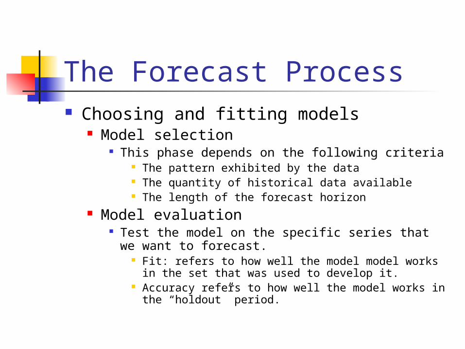
The Forecast Process Choosing and fitting models

Model selection This phase depends on the following criteria

The pattern exhibited by the data The quantity of historical data available The length of the forecast horizon

Model evaluation Test the model on the specific series that we want to forecast.

Fit: refers to how well the model model works in the set that was used to develop it.

Accuracy refers to how well the model works in the “holdout” period.

The Forecast Process Using and evaluating a forecasting model

Forecast preparation The result of having found model or models that you believe

will produce an acceptably accurate forecast. Forecast Presentation

It involve clear communication. Tracking results

Over time, even the best of models are likely to deteriorate in terms of accuracy and should be adjusted or replaced with alternative methods.

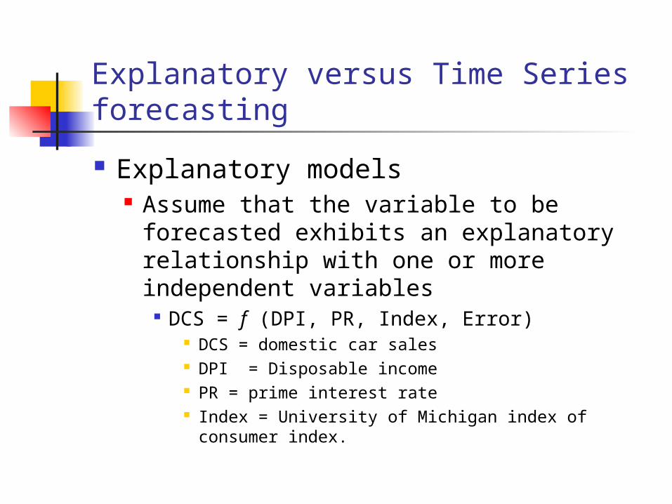
Explanatory versus Time Series forecasting

Explanatory models Assume that the variable to be forecasted

exhibits an explanatory relationship with one or more independent variables

DCS = f (DPI, PR, Index, Error) DCS = domestic car sales DPI = Disposable income PR = prime interest rate Index = University of Michigan index of consumer index.

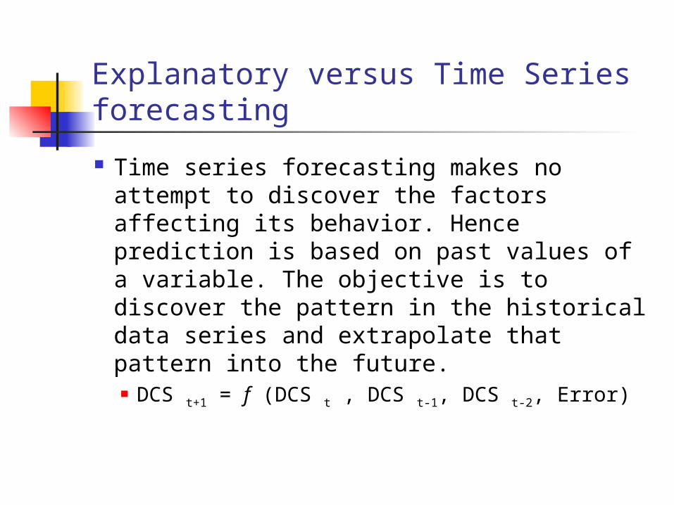
Explanatory versus Time Series forecasting

Time series forecasting makes no attempt to discover the factors affecting its behavior. Hence prediction is based on past values of a variable. The objective is to discover the pattern in the historical data series and extrapolate that pattern into the future. DCS t+1 = f (DCS t , DCS t-1, DCS t-2, Error)

Trend, Seasonal, and Cyclical Data Patterns

The data that are used most often in forecasting are time series.

Time series data are collected over successive increments of time.

Example: Monthly unemployment rate, The quarterly gross domestic product, the number of visitors to a national park every year for a 30-year period.

Such time series data can display a variety of patterns when plotted over time.

Data Pattern A time series is likely to contain some or all

of the following components: Trend Seasonal Cyclical Irregular

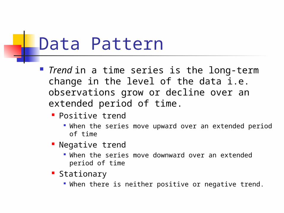
Data Pattern Trend in a time series is the long-term change in

the level of the data i.e. observations grow or decline over an extended period of time. Positive trend

When the series move upward over an extended period of time Negative trend

When the series move downward over an extended period of time

Stationary When there is neither positive or negative trend.

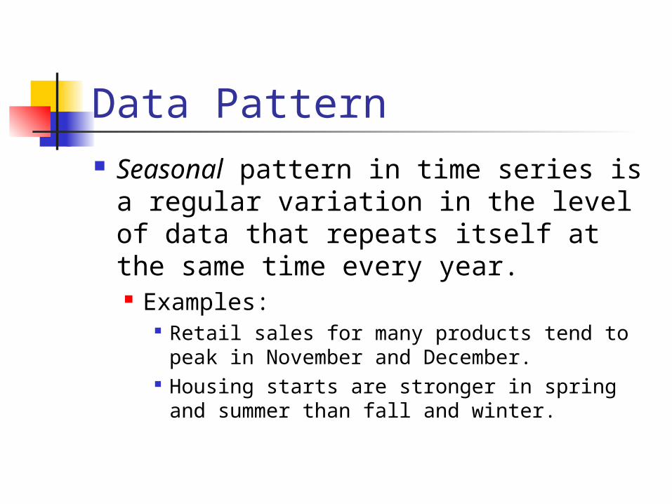
Data Pattern Seasonal pattern in time series is a regular

variation in the level of data that repeats itself at the same time every year. Examples:

Retail sales for many products tend to peak in November and December.

Housing starts are stronger in spring and summer than fall and winter.

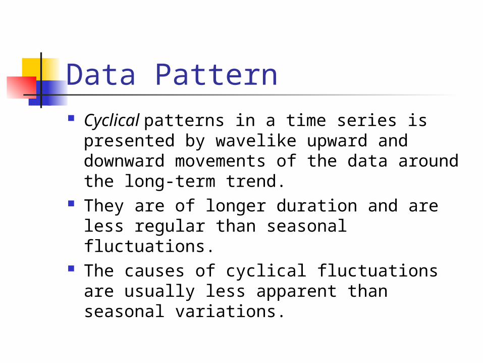
Data Pattern Cyclical patterns in a time series is presented by

wavelike upward and downward movements of the data around the long-term trend.

They are of longer duration and are less regular than seasonal fluctuations.

The causes of cyclical fluctuations are usually less apparent than seasonal variations.

Data Pattern Irregular pattern in a time series data are the

fluctuations that are not part of the other three components

These are the most difficult to capture in a forecasting model

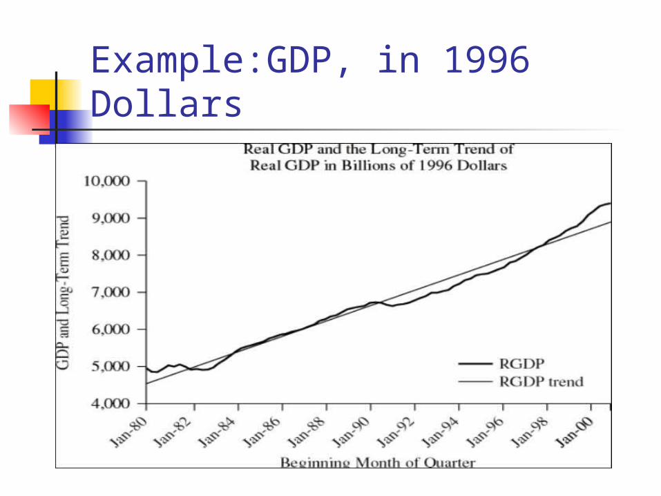
Example:GDP, in 1996 Dollars

Example:Quarterly data on private housing starts

Example:U.S. billings of the Leo Burnet advertising agency

Data Patterns and Model Selection The pattern that exist in the data is an important

consideration in determining which forecasting techniques are appropriate.

To forecast stationary data; use the available history to estimate its mean value, this is the forecast for future period.

The estimate can be updated as new information becomes available.

The updating techniques are useful when initial estimates are unreliable or the stability of the average is in question.

Data Patterns and Model Selection

Forecasting techniques used for stationary time series data are: Naive methods Simple averaging methods, Moving averages Simple exponential smoothing autoregressive moving average(ARMA)


Methods used for time series data with trend are: Moving averages Holt’s linear exponential smoothing Simple regression Growth curve Exponential models Time series decomposition Autoregressive integrated moving average(ARIMA)

Data Patterns and Model Selection For time series data with seasonal component the goal

is to estimate seasonal indexes from historical data. These indexes are used to include seasonality in

forecast or remove such effect from the observed value.

Forecasting methods to be considered for these type of data are: Winter’s exponential smoothing Time series multiple regression Autoregressive integrated moving average(ARIMA)


Cyclical time series data show wavelike fluctuation around the trend that tend to repeat.

Difficult to model because their patterns are not stable.

Because of the irregular behavior of cycles, analyzing these type data requires finding coincidental or leading economic indicators.


Forecasting methods to be considered for these type of data are: Classical decomposition methods Econometric models Multiple regression Autoregressive integrated moving average

(ARIMA)

Example:GDP, in 1996 Dollars

For GDP, which has a trend and a cycle but no seasonality, the following might be appropriate: Holt’s exponential smoothing Linear regression trend Causal regression Time series decomposition

Example:Quarterly data on private housing starts

Private housing starts have a trend, seasonality, and a cycle. The likely forecasting models are: Winter’s exponential smoothing Linear regression trend with seasonal

adjustment Causal regression Time series decomposition

Example:U.S. billings of the Leo Burnet advertising agency

For U.S. billings of Leo Burnett advertising, There is a non-linear trend, with no seasonality and no cycle, therefore the models appropriate for this data set are: Non-linear regression trend Causal regression

Autocorrelation Correlation coefficient is a summary

statistic that measures the extent of linear relationship between two variables. As such they can be used to identify explanatory relationships.

Autocorrelation is comparable measure that serves the same purpose for a single variable measured over time.

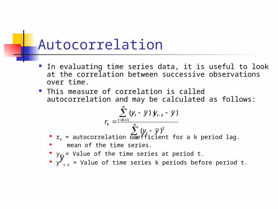
Autocorrelation In evaluating time series data, it is useful to look at the correlation

between successive observations over time. This measure of correlation is called autocorrelation and may be

calculated as follows:

rk = autocorrelation coefficient for a k period lag. mean of the time series. yt = Value of the time series at period t. y t-k = Value of time series k periods before period t.

n

tt

n

ktktt

k

yy

yyyyr

1

2

1

)(

))((

y

Autocorrelation

Autocorrelation coefficient for different time lags can be used to answer the following questions about a time series data. Are the data random?

In this case the autocorrelations between yt and y t-k for any lag are close to zero. The successive values of a time series are not related to each other.

Correlograms: An Alternative Method of Data Exploration

Is there a trend? If the series has a trend, yt and y t-k are highly

correlated The autocorrelation coefficients are significantly

different from zero for the first few lags and then gradually drops toward zero.

The autocorrelation coefficient for the lag 1 is often very large (close to 1).

A series that contains a trend is said to be non-stationary.


Is there seasonal pattern? If a series has a seasonal pattern, there will be a

significant autocorrelation coefficient at the seasonal time lag or multiples of the seasonal lag.

The seasonal lag is 4 for quarterly data and 12 for monthly data.


Is it stationary? A stationary time series is one whose basic

statistical properties, such as the mean and variance, remain constant over time.

Autocorrelation coefficients for a stationary series decline to zero fairly rapidly, generally after the second or third time lag.


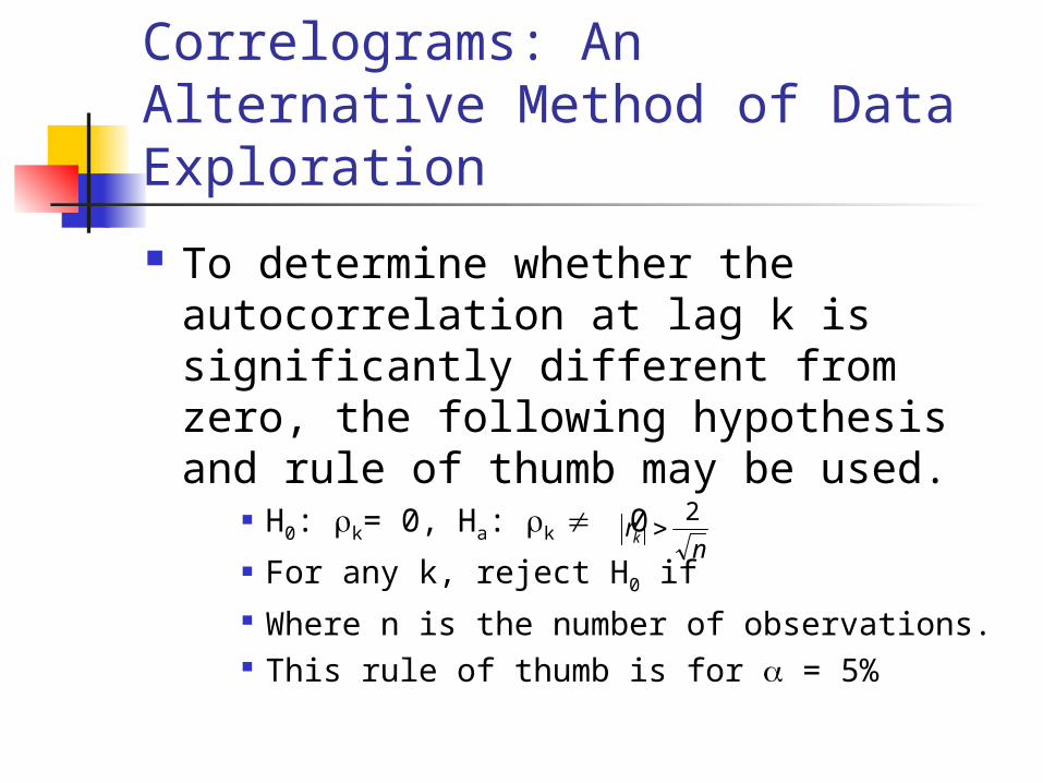
To determine whether the autocorrelation at lag k is significantly different from zero, the following hypothesis and rule of thumb may be used.

H0: k= 0, Ha: k 0

For any k, reject H0 if Where n is the number of observations. This rule of thumb is for = 5%

nrk

2


The hypothesis test developed to determine whether a particular autocorrelation coefficient is significantly different from zero is:

Hypotheses H0: k= 0, Ha: k 0

Test Statistic:kn

rt k

1

0


Reject H0 if

2;2; or knkn tttt


The plot of the autocorrelation Function (ACF) versus time lag is called Correlogram.

The horizontal scale is the time lag The vertical axis is the autocorrelation

coefficient. Patterns in a Correlogram are used to analyze

key features of data.

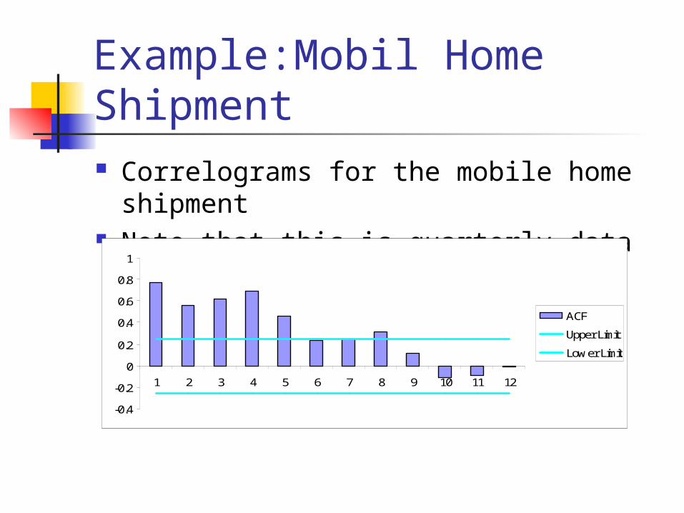
Example:Mobil Home Shipment Correlograms for the mobile home shipment Note that this is quarterly data

-0.4

-0.2

0

0.2

0.4

0.6

0.8

1

1 2 3 4 5 6 7 8 9 10 11 12

ACF

Upper Limit

Lower Limit

Example:Japanese exchange Rate As the world’s economy becomes increasingly

interdependent, various exchange rates between currencies have become important in making business decisions. For many U.S. businesses, The Japanese exchange rate (in yen per U.S. dollar) is an important decision variable. A time series plot of the Japanese-yen U.S.-dollar exchange rate is shown below. On the basis of this plot, would you say the data is stationary? Is there any seasonal component to this time series plot?

Example:Japanese exchange Rate

Japanese Exchange Rate

0

20

40

60

80

100

120

140

160

180

0 5 10 15 20 25 30

Months

Exc

han

ge

Rat

e ( ye

n p

er U

.S. d

olla

r)

EXRJ

Example:Japanese exchange Rate Here is the autocorrelation

structure for EXRJ. With a sample size of 12,

the critical value is

This is the approximate 95% critical value for rejecting the null hypothesis of zero autocorrelation at lag K.

Obs ACF1 .81572 .53833 .27334 .03405 -.12146 -.19247 -.21578 -.19789 -.121510 -.121711 -.182312 -.2593

408.024

22

n

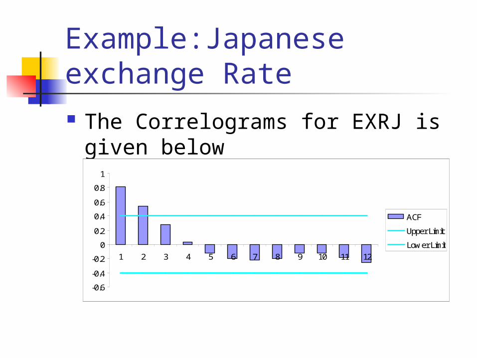
Example:Japanese exchange Rate The Correlograms for EXRJ is given below

-0.6

-0.4

-0.2

0

0.2

0.4

0.6

0.8

1

1 2 3 4 5 6 7 8 9 10 11 12

ACF

Upper Limit

Lower Limit

Example:Japanese exchange Rate Since the autocorrelation coefficients fall to

below the critical value after just two periods, we can conclude that there is no trend in the data.

Example:Japanese exchange Rate

To check for seasonality at = .05 The hypotheses are:

H0; 12 = 0 Ha:12 0

Test statistic is:

Reject H0 if

899.01224/1

2595.

1

0

kn

rt k

2;2; or knkn tttt 179.2025.0;122; tt kn

Example:Japanese exchange Rate Since

We do not reject H0 , therefore seasonality does not appear to be an attribute of the data.

179.2899.0 025.0;12 tt

ACF of Forecast Error The autocorrelation function of the forecast

errors is very useful in determining if there is any remaining pattern in the errors (residuals) after a forecasting model has been applied.

This is not a measure of accuracy, but rather can be used to indicate if the forecasting method could be improved.

Documents

Applied Business Forecasting and Planning The Forecast Process, Data Considerations, and Model Selection