Embed Size (px)
Citation preview

Universita degli Studi di Padova
DIPARTIMENTO DI DI INGEGNERIA DELL’INFORMAZIONE
Corso di Laurea in Ingegneria dell’Automazione
TESI DI LAUREA MAGISTRALE
Applications Oriented Optimal InputDesign: An Analysis of a quadruple water
tank process
Laureando
Antonio BalseminRelatore
Prof. Giorgio Picci
Anno Accademico 2012-2013


Abstract
Model predictive control (MPC) has become an increasingly popular control
strategy thanks to its ability to handle multivariable systems and constraints.
This control technique makes use of a model of the system, therefore perfor-
mances are highly dependent on the accuracy of the model chosen. The process
of obtaining the model is often costly, for this reason system identification
for MPC is an important topic. Applications oriented optimal input design
enables optimization of the system identification experiments, leading to a set
of models with the necessary accuracy for the intended application. In this
thesis a method of system identification for MPC applications is simulated
on a multivariable nonlinear system consisting of four interconnected water
tanks. An analysis of the impact of MPC settings, such as active or no active
constraints and different weight settings, is carried out. The initial hypothesis
is that different MPC settings influence the obtained set of models. Simulations
show that the hypothesis is correct and the result give rise to some interesting
interpretations.

Acknowledgements
Writing my master thesis at KTH it was a great experience. I would like to
thank many people for their support during all the time I worked on my thesis.
First of all I want to thank my italian supervisor Prof. G. Picci who gave me
the possibility to do my thesis at KTH. I would like to thank my examiner
Prof. Bo Wahlberg who introduced me with really interesting research topics
and gave me insightful comments. Special thanks to my supervisors Mariette
Annergren and Christian Larsson for kindness and availability, for patience and
help during all the time I worked on my thesis. This thesis would not exist
without your guidance. Thanks to all the people of the Automatic Control Lab,
for the exciting and inspiring work environment. It was really nice to attend
your meetings. Thanks to Damiano Varagnolo for the useful LATEXtips and
support in general. Many thanks to the administration personal Gustafsson
Kristina, Strom Anneli and Holmqvist Hanna for making sure that we always
had what we need for our work. Thanks to Francesco and Sky, their company
was fundamental during all the time I spent in Sweden.
Finally I want to thank my family for their love and support, for their faith
and for giving me the possibility to have this beautiful experience.

Contents
1 Introduction 1
1.1 Main Topics . . . . . . . . . . . . . . . . . . . . . . . . . . . . . 1
1.2 Problem formulation . . . . . . . . . . . . . . . . . . . . . . . . 3
1.3 Related Work . . . . . . . . . . . . . . . . . . . . . . . . . . . . 3
1.4 Thesis outline . . . . . . . . . . . . . . . . . . . . . . . . . . . . 5
2 Background 7
2.1 Convex Optimization . . . . . . . . . . . . . . . . . . . . . . . . 7
2.1.1 Optimization software . . . . . . . . . . . . . . . . . . . 8
2.2 Model predictive control . . . . . . . . . . . . . . . . . . . . . . 8
2.3 System identification . . . . . . . . . . . . . . . . . . . . . . . . 11
2.4 Identification with a control objective . . . . . . . . . . . . . . . 14
2.5 Applications oriented optimal input design . . . . . . . . . . . . 16
3 Experiment design for model predictive control 21
3.1 Application cost . . . . . . . . . . . . . . . . . . . . . . . . . . . 21
3.2 Identification experiments . . . . . . . . . . . . . . . . . . . . . 24
3.2.1 Identification algorithm . . . . . . . . . . . . . . . . . . . 24
3.3 Sensitivity analysis . . . . . . . . . . . . . . . . . . . . . . . . . 26
3.3.1 Important directions . . . . . . . . . . . . . . . . . . . . 26
3.3.2 Area . . . . . . . . . . . . . . . . . . . . . . . . . . . . . 26
4 The quadruple water tanks process 29
4.1 Process description . . . . . . . . . . . . . . . . . . . . . . . . . 29
4.2 Valves setting and physical interpretation . . . . . . . . . . . . . 33
4.3 Water level control using MPC . . . . . . . . . . . . . . . . . . 35
4.3.1 MPC weights . . . . . . . . . . . . . . . . . . . . . . . . 35

iv Contents
4.3.2 Reference . . . . . . . . . . . . . . . . . . . . . . . . . . 36
4.3.3 handling constraints . . . . . . . . . . . . . . . . . . . . 36
5 Simulations 41
5.1 Minimum phase setting: γ1 = γ2 = 0.625 . . . . . . . . . . . . . 44
5.1.1 Scenario 1 . . . . . . . . . . . . . . . . . . . . . . . . . . 44
5.1.2 Scenario 2 . . . . . . . . . . . . . . . . . . . . . . . . . . 48
5.1.3 Scenario 3 . . . . . . . . . . . . . . . . . . . . . . . . . . 52
5.1.4 Scenario 4 . . . . . . . . . . . . . . . . . . . . . . . . . . 55
5.2 Minimum phase setting: γ1 = γ2 = 0.505 . . . . . . . . . . . . . 58
5.2.1 Scenario 1 . . . . . . . . . . . . . . . . . . . . . . . . . . 58
5.2.2 Scenario 2 . . . . . . . . . . . . . . . . . . . . . . . . . . 62
5.2.3 Scenario 3 . . . . . . . . . . . . . . . . . . . . . . . . . . 64
5.2.4 Scenario 4 . . . . . . . . . . . . . . . . . . . . . . . . . . 66
5.3 Non minimum phase case: γ1 = γ2 = 0.25 . . . . . . . . . . . . . 68
5.3.1 Observation . . . . . . . . . . . . . . . . . . . . . . . . . 68
6 Discussion 69
6.1 Estimates offset . . . . . . . . . . . . . . . . . . . . . . . . . . . 71
7 Conclusions and future work 75
References . . . . . . . . . . . . . . . . . . . . . . . . . . . . . . . . . 77
References 77
Index 79

1Introduction
This master’s thesis project was carried out at the Department of Automatic
Control, Royal Institute of Technology and is based on the research of the
PhD. Students Christian Larsson and Mariette Annergren. The needs to verify
the theoretical results of their research on a concrete and interesting control
problem is the motivation for this project work.
1.1 Main Topics
The main topics of this Master Thesis Project are model predictive control,
system identification, optimal input design and convex optimization.
Model predictive control (MPC) is a particular type of controller which makes
use of an internal model to predict the behaviour of the controlled system,
starting at the current time, over a future prediction horizon. The predicted
behavior depends on the input trajectory that is to be applied over the prediction
horizon. The idea is to select the input that gives the best predicted behavior,
that, at the same time, minimize a function cost. At each step, the whole
input trajectory is computed but only the first element of it is applied to the

2 Introduction
system. At the next step this procedure is repeated, [16]. As we said, the MPC
controller has an internal model, that is used to describe the real system. The
accuracy of the model, affects the control performance of the MPC. Procedures
involving system identification are often used to construct the model.
“System identification deals with the problem of building mathematical models
of dynamical systems based on observed data from the system”, [15]. The
goal is to find a model M that describes the relevant properties of the studied
system S. The main steps of the identification process is to:
• collect data from the system (inputs and outputs),
• define a set of candidate models, choosing a model structure,
• choose a criterion by which candidate models can be assigned using the
data,
• estimate parameter values based on data, structure and criterion,
• validate the model.
The validation step involves various procedures to assess how the model is
related to observed data. If a model does not pass the model validation test,
we must go back and revise the various steps of the procedure.
Optimal input design relates to finding the input signal that assures that
the estimates become as good as possible. The traditional way to obtain an
informative experiment is to minimize the covariance matrix of the estimated
parameter vector. However, in application oriented input design, [12], [8], et
cetera, the focus is shifted towards the application of the estimated model.
Instead of the covariance matrix of the estimated parameter vector, the distance
between nominal performance and performance achieved with the model is
considered.
Convex optimization is a class of mathematical optimization. In this class, the
objective and the constraint functions have to be convex. General optimization
problems can be very difficult to solve or even intractable. Moreover if they are
solvable, they can require very long computation time. Convex optimization
problems, on the other hand, are solvable and the solutions can be found
efficiently and reliably. For these good qualities one should always rewrite an
optimization problem in convex form, whenever possible.

1.2 Problem formulation 3
1.2 Problem formulation
For controllers based on a model of the system, the accuracy of the model is
crucial. Mathematical models can not perfectly describe the systems they are
meant to describe. This discrepancy is called plant-model mismatch. When a
specific application is considered, usually not all system properties have the
same importance. Hence it is crucial that the model used by the controller
captures the system properties important for the intended application. These, in
fact, affect the control performance more evidently. The quality of the estimated
models is affected by the input used in the identification experiment. Optimal
input design is used as a tool, to obtain an input signal that uses as little
resources as possible, while guaranteeing that the performance specifications in
the intended application are met. Thus giving a set of acceptable models. This
problem is formulated as follows [12]
minimizeinput
Experimental effort
subject to Performance specifications(1.1)
Within the framework described, we consider a particular nonlinear system
composed by four interconnected water tanks controlled by MPC. This system
has the ability to change one zero location, from minimum phase to non
minimum phase by simply acting on a physical parameter. An analysis of the
impact of MPC settings, such as active or no active constraints and different
weight settings, is carried out.
1.3 Related Work
The research performed by Prof. Bo Wahlberg [18], and Prof. Hakan Hjalmars-
son [8], deals with experiment design for system identification (more references
in this field can be found in the references of [18] and [8]). They combine the
criterion, that the model should fulfil in the system identification process, with
the requirements on the system’s behaviour in the control theory problem. In
[8] the cost of complexity is defined as the minimum possible experimental
effort required to obtain a parameter estimate that guarantees the desired
performance in the control application. Furthermore, it was underlined that
the identification experiments should reveal system properties important for
4 Introduction
the application and conceal irrelevant properties.
The identification experiment can be performed in open loop or in closed loop.
Open loop identification is when there is no feedback control of the system
during the identification experiment. Closed loop identification is when there
is feedback control. Methods for optimal input design in system identification
for control with open loop identification have been extensively treated in [8],
[14], [13], [12], [19].
In [19] model based control design methods, such as MPC, where the model is
obtained by means of the prediction error system identification method, are
studied. The accuracy of the model used in this control method is a main
issue, as it is strictly related to degradation in control performance. Control
performance is defined using a cost function that specifies which parameter val-
ues give acceptable performance. The objective is to find a minimum variance
input signal to be used in the system identification experiment, such that the
control performance specification is fulfilled with a given probability when using
the estimated model in the control design. This problem can be reformulated
as a convex optmization problem. Examples with FIR models show that up
to a factor two in input power can be gained when using the optimal input
compared to white noise. Other examples, show that much higher gain can be
obtained in input power.
MPC applications are discussed more in [13], where a water tank process is
considered. A scheme for optimal input design in a MPC context is presented,
the major challenges with the practical implementation are highlighted, and
an algorithm for identification experiments is proposed. It is also pointed
out that there is no good way to consider time domain constraints in the
identification part of the method, but they can be included in the calculation
of the application cost.
Thanks to the work of Mariette Annergren and Christian Larsson a Model
Based Optimal Input Design Toolbox for Matlab (MOOSE) has been developed,
[4]. It simplifies the implementation of optimal input design problems, providing
an extra layer between the user and CVX, a package for specifying and solving
convex programs [7, 6]. At the time of writing, MOOSE only handles open
loop identification.

1.4 Thesis outline 5
1.4 Thesis outline
The thesis is organised in Chapters. In Chapter 2 treats the background.
Chapter 3 focuses on the application oriented optimal input design in an MPC
context. In Chapter 4 the quadruple water tank system is described. In
Chapter 5 are presented the results obtained from the simulations, results are
briefly described. A more detailed analysis and comparisons of the results, are
presented in Chapter 6.

6 Introduction

2Background
2.1 Convex Optimization
A convex optimization problem can be written in the following form,
minimizex
f(x)
subject to gi ≤ 0, i = 1, . . . ,m(2.1)
where the functions f and g are convex. A particular kind of these problems is
the so called Semi Definite Program (sdp) in which the objective function f is
linear and the inequality constraints gi ≤ 0 are called Linear Matrix Inequalities
(lmi). These problems have the following form
minimizex
cTx
subject to x1F1 + x2F2 + · · ·+ xnFn +G � 0,(2.2)
where Fi, G ∈ Sk and Sk is a set of k × k symmetric matrices. In (2.2) it is
possible to include multiple lmi constraints. For example the two constraints,
x1F1 + x2F2 + · · ·+ xnFn +G � 0, x1H1 + x2H2 + · · ·+ xnHn +R � 0,

8 Background
can be rewritten in a single lmi constraint as follows
x1
[F1 0
0 H1
]+ x2
[F2 0
0 H2
]+ · · ·+ xn
[Fn 0
0 Hn
]+
[G 0
0 R
]� 0.
Convex problems have the important property that if a solution is found, it
is guaranteed to be globally optimal. Convex optimization problems can be
solved reliably and efficiently, using one of the available optimization solvers.
A very extensive reference to deepen the knowledge about convex optimization
is [3].
2.1.1 Optimization software
Prof. Stephen Boyd and Dr. Michael Grant at the Department of Electrical
Engineering, Stanford University, have developed a programming framework
for convex optimization problems called cvx, [7]. It is implemented in the
software Matlab and uses Matlab-syntax.
The PhD. Students Mariette Annergren and Christian Larsson developed a
Matlab Toolbox for optimal input design called MOOSE, [4]. MOOSE is a
model based optimal input design toolbox which simplify implementation of
optimization problems found in input design. It provides an extra layer between
the user and a convex optimization environment. For the flexibility and easy
setting up of optimization problems this toolbox was used in this master thesis
project.
2.2 Model predictive control
Model predictive control is a control method which has made a significant
impact on control of industrial processes, especially in the petrochemical
industry. In fact, most petrochemical plants and refineries have implemented
MPC [21]. Due to increased microprocessor speeds, MPC is spreading out into
other application fields. For example, for controlling heating and ventilation
systems in buildings. Main reasons that prompt the use of MPC are the simple
treatment of multivariate processes and the ability to handle constraints on
state variables and signals. Constraints can arise from physical limitations of
the plant (consider for example saturation limits due to actuators), or they

2.2 Model predictive control 9
can be of different nature as desired accuracy in product specifications or
economical effort, et cetera.
At the core of any MPC implementation there is a model of the process that
has to be controlled. Typically the model is a linear, in discrete time model,
and can be written as,
x(t+ 1) = Ax(t) + Bu(t) + v(t),
y(t) = Cx(t) + w(t).(2.3)
Here x(t) ∈ Rn is the state vector, u(t) ∈ Rm is the controlled input signal,
y(t) ∈ Rp the measured output, and v(t) and w(t) are stationary, zero-mean,
white signals commensurate with x(t) and y(t).
The MPC makes use of a model of the system and the measured data from the
system to predict the system’s future output signals, as a function of future
input signals. The predicted inputs and outputs are used in an objective
function, that penalizes undesired behavior, and it is minimized with respect
to the future input sequence. When an optimal input trajectory is obtained,
just the first element of the sequence is applied to the system. The procedure
is then repeated at the next time step.
A key feature of MPC is that constraints on states, inputs and outputs can easily
be taken into account using constrained optimization methods. The control
input is computed, optimizing an objective function over a future prediction
horizon. The prediction horizon, denoted Ny, defines the number of samples of
the output that are predicted and the control horizon, denoted Nu, defines the
number of samples of the input that are used in the optimization algorithm.
The predicted behaviour of the system, that is y(t + i|t) for i = 1, · · ·Ny,
depends on the assumed input trajectory u(t + i|t) for i = 0, · · · , Nu − 1,
that is used over the control horizon. At time t it is assumed to collect the
measurement y(t) and the input u(t|t) is computed at the same time sample.
Once a future input trajectory has been chosen, only the first element of this it
is applied to the system, that is u(t) = u(t|t). In the next time sample, a new
measurement of the output is collected and the whole cycle of prediction of
output and evaluation of the input trajectory is repeated. The length of the
prediction and control horizons remain the same in each iteration, but they are
shifted one time step ahead. This control technique is often called a receding
horizon strategy.

10 Background
Figure 2.1: The receding horizon idea, [1]. In the upper figure at time t an input trajectoryis evaluated (here p correspond to control horizon Nu) but only the first element is appliedin the system as shown in the lower figure. At time t+ 1 a new optimal control is evaluated.
A common choice for the objective function used in MPC is [16]
J(t) =
Ny∑
i=0
‖ y(t+ i|t)− r(t+ i) ‖2Qy
+Nu∑
i=0
‖ ∆u(t+ i) ‖2Qu
(2.4)
where y(t+ i|t) is the predicted output, r(t) is the reference and ∆u(t+ i) =
u(t+ i)− u(t+ i− 1) is the increment of the input at time t. The norm ‖ x ‖Ais equal to
√xTAx. The weighting matrices Qy and Qu, which are usually
diagonal matrices, are tunable parameters.
The general optimization problem in MPC can be formulated as
minimizeu(t),u(t+1),··· ,u(t+Nu)
J(t)
subject to y(t), y(t+ 1), · · · , y(t+Ny) ∈ Yu(t), u(t+ 1), · · · , u(t+Nu) ∈ U
(2.5)
where Y and U represent the constraint sets for outputs and inputs respectively.
The MPC problem as presented above can be formulated as a Quadratic Problem
(QP) for which highly reliable and efficient solvers are available. The design
parameters of the MPC are
• the model used in the MPC (matrices A, B and C);
• prediction and control horizon Np and Nu;
• weighting matrices Qy and Qu;

2.3 System identification 11
• constraints on inputs, umin, umax (which are usually given by the system,
e.g. saturations in actuators);
• constraints on outputs, ymin, ymax (which are usually imposed, e.g. by
safety limits).
Most important to ensure good performance of the MPC is to have a model
that describe with high accuracy the important properties of the system that
has to be controlled. Plant-model mismatch can cause constraints violation or
even instability in reference tracking applications. If a nonlinear system has to
be controlled with MPC a linearized model, around an equilibrium point, has
to be provided.
2.3 System identification
System identification is the process of constructing models of dynamic systems
from experimental data. The goal is to find a model M belonging to a given
class of parametric models that describes the relevant properties of the studied
system S. Identification experiments can be performed in open loop or in closed
loop. In open loop identification there is no feedback control of the system
during the identification experiment while in closed loop we have feedback
control during the identification experiment. In this thesis all identification
experiments are performed in open loop.
In the context considered in this thesis, the systems we want to identify are
linear time-invariant, asymptotically stable multivariate systems on the form
S :x(t+ 1) = Ax(t) + Bu(t) + v(t)
y(t) = Cx(t) + w(t)(2.6)
with known input u(t) and measured output y(t). The noises v(t) and w(t)
are white, zero-mean stationary processes with covariance matrices Λv and Λw.
They are called process noise and measurement noise, respectively. Different
identification methods are possible for finding the modelM. Such methods can
be parametric or non-parametric and can be performed in both time domain
or frequency domain. In this thesis we consider a parametric time domain
12 Background
identification method. The model structure is
M(θ) :x(t+ 1, θ) = A(θ)x(t, θ) + B(θ)u(t) + K(θ)e(t)
y(t, θ) = C(θ)x(t, θ) + e(t),(2.7)
where θ ∈ Rn represents the unknown parameter vector to be identified and
e(t) is a zero-mean, white process with covariance matrix Λe. It is assumed
that the model class M(θ) include the true system. That is, there exists a
true parameter vector θ0 such that S =M(θ0). The model structure in (2.7)
is in innovation form. That it is not restrictive since it is always possible to
transform a state space representation to the innovation form. Indeed a model
on the same form as (2.6) can be rewritten in innovation form using spectral
factorization. We must solve the Riccati equation
P (θ) = A(θ)P (θ)AT (θ) + Λv(θ)− [A(θ)P (θ)CT (θ) + S(θ)]
× [C(θ)P (θ)CT (θ) + Λw(θ)]−1[C(θ)P (θ)AT (θ) + ST (θ)].
Where S(θ) = EvwT . The solution P (θ) is a symmetric positive definite matrix.
With P (θ) one can compute the Kalman gain
K(θ) = [A(θ)P (θ)CT (θ) + S(θ)][C(θ)P (θ)C(θ)T + Λw(θ)]−1,
thus obtaining a model of the same form as (2.7). The estimates of θ are found
using the prediction error method [15], this method and the properties of the
resulting estimates are summarized next.
Prediction error method
Given a modelM(θ) belonging to a parametric class of models and a sequence
of input-output data
yN = {y(t); t = 1, 2, ..., N} , uN = {u(t); t = 1, 2, ..., N} ,
this method can be summarized as follows [17],
1. For a general value of θ the one step ahead predictor is constructed. If a
model of the form (2.7) is used, the one step ahead predictor is given by

2.3 System identification 13
[15]
x(t+ 1, θ) = A(θ)x(t, θ) + B(θ)u(t) + K(θ)(y(t)− y(t, θ)),
y(t, θ) = C(θ)x(t, θ).(2.8)
2. The prediction errors are constructed
εθ(t) = y(t)− y(t, θ), t = 1, 2, ...N.
3. The parameter estimate is found minimizing a cost function represented
for example by
VN(θ) =1
N
N∑
t=1
εθ(t)2 (2.9)
minimizing (2.9). The parameter vector estimate is obtained as
θN = argminθ
VN(θ) (2.10)
4. The variance of innovation λ = var {e(t)} estimate is obtained evaluating
the (2.9) at the parameter estimate vector θN
λN = VN(θN)
To determine how good this method is, we look at its asymptotic properties.
That is, when the number of samples used in the identification experiment goes
to infinity.
As stated in [15], we assume that the (true) process can be described by a
model M(θ). Under mild assumptions on the data, and model, and the cost
function chosen as in (2.9), then the PEM estimator is consistent, or in other
terms,
limN→∞
θN = θ0 w.p.1 (2.11)

14 Background
Furthermore the asymptotic distribution is given by [15]
√N(θN − θ0) ∈ N (0,P) as N →∞, (2.12a)
P =[E{ψ(t, θ0)Λ−1
e ψT (t, θ0)}]−1
, (2.12b)
ψ(t, θ0) =dy(t)
dθ
∣∣∣∣θ=θ0
. (2.12c)
The X 2-distribution can be used to describe the estimates convergence. In
fact, if we consider a variable y ∼ N (µ,Σ) with mean µ ∈ Rm and covariance
matrix Σ ∈ Rm×m positive definite, then it holds that
(y − µ)TΣ−1(y − µ) ∼ X 2(m),
where the number of degrees of freedom of the X 2 distribution, is given by the
dimension of y. An α-level confidence ellipsoid (that we call the identification
ellipsoid) for the estimated parameters is given by [8]
ESI(α) =
{θ : [θ − θ0]TP−1[θ − θ0] ≤ X
2α(n)
N
}. (2.13)
The constant X 2α(n) is the α-percentile of the X 2 distribution with n degrees
of freedom. This means that if the number of samples N is sufficiently large
the identification ellipsoid will contain θN with probability α. The confidence
ellipsoids will prove to be useful in the optimal input design.
2.4 Identification with a control objective
A controller based on a model of the system will achieve good performance if
the accuracy of the identified model used by the controller (in the important
directions of the parameter space) is high. The concept of important direction
will be clarified in Section 3.3.1. The objective of optimal input design is to
deliver a model that when used in the intended application will give acceptable
performance. To have a measure of degradation of control performance, and
to be able to define acceptable performance in the intended application, an
application cost function is used, see [8]. Since the models considered are
parametrized by the vector θ, the application cost becomes a function of θ. If
an exact mathematical model of the true system was available, that is, if θ0 was
2.4 Identification with a control objective 15
known, the desired performance would be obtained. However, when the model
does not correspond to the true system, the mismatch can cause a degradation
in the controller performance.
Definition 2.4.1. (Application cost, [12]) If θ ∈ Rn is a parameter vector
corresponding to the model M(θ), and S =M(θ0), the function
Vapp(θ) : Rn → R+, (2.14)
is an application cost if it has the following properties,
Vapp(θ0) = 0, V′app(θ0) = 0, V
′′app(θ0) � 0, (2.15)
The application cost gives a scalar number that shows how much performance
degrades when a parameter vector θ is used, instead of the true parameter
vector θ0 in the intended application. In any application there is a maximal
allowed performance degradation, this gives an upper limit of the application
cost that we can express on the form
Vapp(θ) ≤1
γ(2.16)
for some real-valued positive constant γ. This bound gives a set of parameters
that correspond to acceptable application performance.
Definition 2.4.2. (Application set, [12]) If Vapp is an application cost and
γ ∈ R+, the application set is defined as
Θapp(γ) =
{θ : Vapp(θ) ≤
1
γ
}. (2.17)
This leads to the idea that the objective of applications oriented system identi-
fication should be to deliver parameter estimates that belong to the application
set.

16 Background
2.5 Applications oriented optimal input
design
As stated in [12], the objective of applications oriented optimal input design is
to find an input that with high probability α, results in acceptable parameters θ,
that satisfy condition (2.16), while at the same time minimizing the experimental
effort of the identification experiment. It is possible to formulate this problem
as followsminimize
inputExperimental effort
subject to P {θ ∈ Θapp(γ)} ≥ α.(2.18)
Meaning, that the aim of the application optimal input design the experimental
effort is to find the input that minimize an experimental effort, while the esti-
mates are acceptable parameters with high probability α. In the optimal input
design problem it is necessary to quantify the experimental effort. Quantifying
experimental effort is not obvious but some common possibilities are to look at
• experiment length, N,
• input power i.e. var {u},
• input energy i.e. N · var {.u}.
In the rest of the thesis focuses on input power. The objective of the optimization
problem (2.18) is defined as [13]
trace
(1
2π
∫ π
−πΦu(ω)dω
)(2.19)
To see the way the input comes into the system identification problem, as a
design variable, it is useful to have a look at the frequency domain expression
of P−1. By Parseval’s theorem, P−1 is given by the following lemma [12].

2.5 Applications oriented optimal input design 17
Lemma 2.5.1. In open-loop identification, the inverse covariance matrix P−1
in (2.13) is an affine function of the input spectrum Φu given by
P−1 =1
2π
∫ π
−πΓ1(ejω)Λ−1
e ⊗ Φu(w)ΓH1 (ejω)dω
+1
2π
∫ π
−πΓ2(ejω)Λ−1
e ⊗ Λe(ω)ΓH2 (ejω)dω,
Γ1(ejω) =
vec F 1u
...
vec F nu
, Γ2(ejω) =
vec F 1e
...
vec F ne
F iu = H(q, θ)
∂G(q, θ)
∂θTi
∣∣∣∣θ=θ0
, i = 1, . . . , n,
F ie = H(q, θ)
∂H(q, θ)
∂θTi
∣∣∣∣θ=θ0
, i = 1, . . . , n,
G(q, θ) = C(θ)(qI −A(θ))−1B(θ),
H(q, θ) = C(θ)(qI −A(θ))−1K(θ) + I.
(2.20)
Where θi represent the i-th component of the vector θ. Furthermore vec X is
the row vector with rows of X stacked next to each other.
A proof of this Lemma can be found in [2]. According to Lemma 2.5.1 and
expression (2.20), it turns out that, in open loop identification, P−1 is an affine
function of the input spectrum Φu. Consequently by a linear parametrization
of the input spectrum, input spectrum constraints can be formulated as lmis,
for details see [9].
Approximation of the application set
It is not guaranteed that in the problem formulation (2.18) the application set,
defined by Vapp(θ) and γ, is convex. But it is possible to use an approximate
description of Θapp(γ) instead. Two different possibilities to do it are presented
in [12]:
• ellipsoidal approximation,
• scenario based approach.
18 Background
Ellipsoidal approximation
Using a second order Taylor expansion of Vapp(θ), this can be approximated
around θ0. According to Definition (2.4.1), Vapp(θ0) = V′app(θ0) = 0, then
Vapp(θ) ≈ Vapp(θ0) + [θ − θ0]T V′app(θ0) +
1
2[θ − θ0]T V
′′app(θ0) [θ − θ0]
=1
2[θ − θ0]T V
′′app(θ0) [θ − θ0] .
(2.21)
Using expression (2.21) in (2.16), the inequality that defines the allowed perfor-
mance degradation can be approximated by
[θ − θ0]T V′′app(θ0) [θ − θ0] ≤ 2
γ. (2.22)
Meaning, that the application set can be approximated by the ellipsoid
Θapp(γ) ≈ Eapp =
{θ : [θ − θ0]T V
′′app(θ0) [θ − θ0] ≤ 2
γ
}. (2.23)
The approximate application set Eapp is called the application ellipsoid, [12]. In
[12] it is also pointed out that for large values of γ (that is for high performance
demands) the approximation will be better than for small values. An example
of an application ellipsoid is provided in Figure 2.2. In this thesis the ellipsoidal
approximation is used.
Scenario based approach
A different approximation is introduced in [14], in an experiment design context.
The approximation is obtained by randomly selecting parameters from Θapp(γ)
to represent the set. Thus, the approximated application set is simply given
by the selected parameters. The more parameters that are selected, the more
accurate the approximation of Θapp(γ) is. This method will not be explained
more in detail, since in this thesis the ellipsoidal approximation will be used
instead.
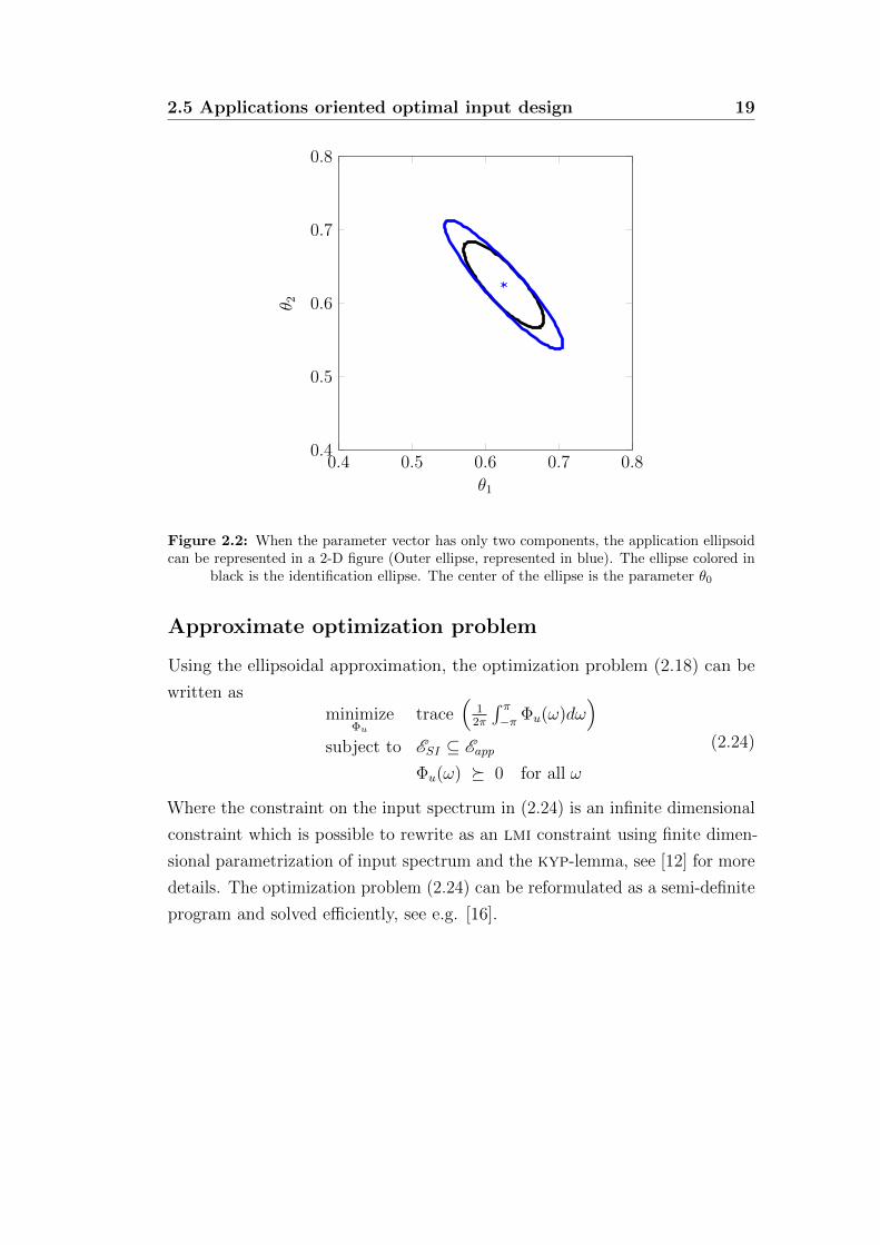
2.5 Applications oriented optimal input design 19
0.4 0.5 0.6 0.7 0.80.4
0.5
0.6
0.7
0.8
θ1
θ 2
Figure 2.2: When the parameter vector has only two components, the application ellipsoidcan be represented in a 2-D figure (Outer ellipse, represented in blue). The ellipse colored in
black is the identification ellipse. The center of the ellipse is the parameter θ0
Approximate optimization problem
Using the ellipsoidal approximation, the optimization problem (2.18) can be
written asminimize
Φu
trace(
12π
∫ π−π Φu(ω)dω
)
subject to ESI ⊆ Eapp
Φu(ω) � 0 for all ω
(2.24)
Where the constraint on the input spectrum in (2.24) is an infinite dimensional
constraint which is possible to rewrite as an lmi constraint using finite dimen-
sional parametrization of input spectrum and the kyp-lemma, see [12] for more
details. The optimization problem (2.24) can be reformulated as a semi-definite
program and solved efficiently, see e.g. [16].

20 Background
3Experiment design for model predictive
control
3.1 Application cost
An application cost is a tool that permits to quantify how good is an estimated
model, if used in a specific application. As seen in Section 2.3 the model
structure of our estimated models is fixed. Hence, evaluating the application
cost for a parameter vector θ, quantifies degradation of performance when that
parameter is used. Furthermore, application cost shows, in which directions, in
the parameter space, the performance is more sensitive to parameters variations.
The analysis gives an insight into which parameters, or combination of them,
that are more important to estimate with high accuracy. As stated in [13], by
calculating the difference between the output of the system controlled by an
MPC, based on a model using θ 6= θ0 and one based on θ0, denoted y(t, θ0) and
y(t, θ) respectively, a reasonable application cost for the MPC case is given by
Vapp(θ) =1
N
N∑
t=1
‖ y(t, θ0)− y(t, θ) ‖2 . (3.1)

22 Experiment design for model predictive control
This function has the desired properties defined in Definition 2.4.1. Usually
it is unlikely that one can know the value of θ0 or try MPCs with different
parameter vectors directly on the true system. Hence in [13] an approximate
application cost, Vapp, is introduced. The true output of the system, y(t, θ0),
is replaced by the output of a linear model that use an estimated parameter
vector θ. This gives,
Vapp(θ, θ) =1
N
N∑
t=1
‖ y(t, θ, θ)− y(t, θ, θ) ‖2 . (3.2)
Where the second argument in (3.2) represents the parameter vector of the
model used by the MPC. The third argument is the parameter vector of the
linear model replacing the true system.
As seen in Section 2.4, to define an application set, it is necessary to set an
upper limit of the application cost, that is to choose a value for γ. The choice is
highly application dependent. In [13], for reference tracking application using
an MPC, allowing for a level of 1 % of degradation in the performance, it is
chosen as
γ =100
V (θ0). (3.3)
Where
V (θ0) =1
N
N∑
t=1
‖ y(t, θ, θ)− r(t) ‖2 . (3.4)

3.1 Application cost 23
0.4 0.45 0.5 0.55 0.6 0.65
0.45
0.5
0.55
0.6
θ1
θ 2
Figure 3.1: Level curves of Vapp(θ) and ellipsoidal approximation of Vapp(θ, θ) centered inθ0. The offset in the direction of the application ellipsoid, can be explained by the fact that,to evaluate Vapp(θ, θ) a linear approximation of the true model is used instead. It is possible
to notice, that the level curves are not ellipses and are not centered in θ0.

24 Experiment design for model predictive control
3.2 Identification experiments
In all simulations that will be presented in Chapter 5 the true system is
represented by a nonlinear model. The nonlinear model is linearized around
an equilibrium point and discretized. This gives a model M(θ0), in the same
form as in (2.7). All identification experiments are performed in open loop.
The models identified have a fixed structure, hence a grey box identification is
performed using the IDGREY and PEM commands of MATLAB.
3.2.1 Identification algorithm
A complete application oriented identification method is presented in [13].
Algorithm
Step 0 Obtain an initial estimate of the model parameters using a white noise
input sequence in the first identification experiment.
Step 1 Find the application cost based on simulations of the model with the
parameter estimates.
Step 2 Design the optimal input signal based on the application cost and param-
eter estimates.
Step 3 Find a new estimate of the model parameters using the optimal input
signal in the system identification experiment.
As stated in [13], if a good initial guess of the parameters is available, for
example coming from physical insight of the process, this guess can replace
the initial estimation in Step 0. Furthermore, in [13] it is pointed out that
the algorithm can be iterated. In fact the estimate from Step 3 can be used,
instead of the initial guess, in Step 1 and 2.
The algorithm is also represented in a block diagram in Figure 3.2. The non
linear model is excited by a white Gaussian noise n with low variance, around
an equilibrium point, to find an initial estimate θ. This initial estimate is used
by an MPC to control a linear modelM(θ) that should represents the linearized
model of the true system. This gives the trajectory y(θ, θ), see Section 3.1.
Another MPC using a parameter θ 6= θ is then used to control the same linear
model M(θ). This gives the trajectory y(θ, θ), see Section 3.1. These two

3.2 Identification experiments 25
trajectory are used to evaluate Vapp(θ, θ). Considering many simulations, for
different values of θ, the hessian matrix V′′app(θ, θ) can be calculated. Based on
the hessian matrix the optimal input design problem is solved. The resulting
input design is optimal forM(θ) but may not be optimal for the true nonlinear
model.
In Chapter 4 this algorithm will be applied to a multivariable process of four
interconnected tanks. In Chapter 5 simulations will be performed, both using
optimal input and white noise input, with different system setups allowing for
comparisons.
MPC(θ)
MPC(θ)
M(θ)
M(θ)
Vapp(θ, θ)
y(θ, θ)
y(θ, θ)
r
MPC simulation
MOOSEV
′′app(θ, θ)
SYS IDSn
y
θ
Φou
Signal generationuopt
S
SYS ID
θ
MPC(θ)
MPC(θ)
M(θ)
M(θ)
Vapp(θ, θ)
y(θ, θ)
y(θ, θ)
r
MPC simulation
MOOSEV
′′app(θ, θ)
SYS IDSn
y
θ
Φou
Signal generationuopt
S
SYS ID
θ
Figure 3.2: Identification Algorithm. An initial identification experiment using a whitegaussian noise n gives an initial parameter vector θ (upper figure). In the lower figure Step1, 2 and 3 of the algorithm are schematically represented. The control performance areevaluated for different values of θ. This is done simulating a model of the system (M(θ))
controlled by an MPC using θ and another MPC using θ. The output trajectories y(θ, θ)and y(θ, θ) are used to evaluate the approximate application cost V
′′
app. This is used by thetoolbox MOOSE to evaluate the optimal input spectrum Φo
u and the with that the optimalinput uopt can be realised. The latter is then used for a new identification experiment giving
a new estimated parameter.
26 Experiment design for model predictive control
3.3 Sensitivity analysis
3.3.1 Important directions
When an estimated parameter vector is used, instead of the true one, the per-
formance degrades. Variations of the estimated parameters from the true ones
cause plant-model mismatch, thus giving worse performance. It is interesting to
notice that not every variation, give the same performance degradation. As seen
in Section 3.1, the application cost can be used, to get in which directions the
performance is more sensitive to parameters’ variations. The analysis is done
considering the application ellipsoid Eapp. As defined in (2.23) the application
ellipsoid is defined by using the hessian of the application cost. When the latter
can not be evaluated (see Section 3.1), V′′app(θ, θ) is used instead.
When we consider a two dimensional parameters vector, the application el-
lipsoid can be represented in a 2-D figure as an ellipse. The lengths of the
semi-axes are given by1√λi
, where λi are the eigenvalues of V′′app(θ, θ). The
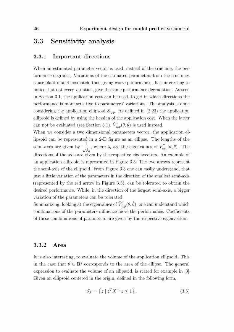
directions of the axis are given by the respective eigenvectors. An example of
an application ellipsoid is represented in Figure 3.3. The two arrows represent
the semi-axis of the ellipsoid. From Figure 3.3 one can easily understand, that
just a little variation of the parameters in the direction of the smallest semi-axis
(represented by the red arrow in Figure 3.3), can be tolerated to obtain the
desired performance. While, in the direction of the largest semi-axis, a bigger
variation of the parameters can be tolerated.
Summarizing, looking at the eigenvalues of V′′app(θ, θ), one can understand which
combinations of the parameters influence more the performance. Coefficients
of these combinations of parameters are given by the respective eigenvectors.
3.3.2 Area
It is also interesting, to evaluate the volume of the application ellipsoid. This
in the case that θ ∈ R2 corresponds to the area of the ellipse. The general
expression to evaluate the volume of an ellipsoid, is stated for example in [3].
Given an ellipsoid centered in the origin, defined in the following form,
EX ={z | zTX−1z ≤ 1
}, (3.5)

3.3 Sensitivity analysis 27
0.55 0.6 0.65 0.7
0.54
0.56
0.58
0.6
0.62
0.64
0.66
0.68
0.7
0.72
Figure 3.3: Application ellipsoid Eapp.
where X = XT � 0, that is, X is symmetric and positive definite. The volume
of the ellipsoid is proportional to (detX−1)12 =
1√λ1 · λ2 · · ·λn
, where n is the
dimension of X.
The area will be used in Chapter 5 to compare application ellipsoids obtained
using different MPC settings.

28 Experiment design for model predictive control
4The quadruple water tanks process
4.1 Process description
The process is composed by four interconnected water tanks, two pumps and
two valves, that divide the water flow in upper and lower tanks. The tanks are
stacked one over each other in couples and numbered as schematically showed
in Figure 4.1. Each tank has a hole at the bottom where water can flow out.
The flow of the two upper tanks goes into the respective lower tank, while
the flow of the two lower tanks goes in a common water container arranged
below the tanks. The pumps are connected in such a way that pump 1 delivers
water to tank 1 and 4, while pump 2 delivers water to tank 2 and 3. The
process has some physical constraints, as described in Table 4.1. The water
level in each tank is measured by pressure sensors at the bottom of the tank.
The sensors are characterized by a conversion constant which is known to be
kc = 0.2 V/cm. The outputs of the process are the pressure sensor signals from
the lower tanks. The inputs of the process are the voltages applied to the two
pumps. Depending on the setting of the two valves one can decide the fraction
of water that will be delivered to the upper tank and to the lower. The valve
setting determines if the process is minimum phase or not.

30 The quadruple water tanks process
Parameter Limit Descriptionhi,max 25 cm Maximum water level of tank ihi,min 0 cm Minimum water level of tank iuj,max 15 V Maximum voltage of pump iuj,min 0 V Minimum voltage of pump i
Table 4.1: Physical constraints of the quadruple tank process.
Nonlinear model
The process is very well described by a system of nonlinear differential equations.
One can express the variation of the volume V of water in each tank with the
following expressiondV
dt= qin − qout (4.1)
where qin and qout represent the total inflow and outflow of water respectively.
The outflow of water of each tank can be found, using Torricelli’s principle1
and given the cross sectional area a of the outlet hole of the tank, to be
qout = a√
2gx, (4.2)
where x is the level of water in the tank and g = 981 cm/s2 is the gravitational
constant.
The inflow of water to the upper tanks, comes from the flow generated from a
pump. For the lower tanks, in addition to the pump flow, there is also the flow
coming from the upper tanks. The outflow q of a pump is proportional to the
applied voltage u, that is q = ku where k is the constant of the pump. The
flow q is then divided into the respective upper and lower tanks, according to
the setting of the valves. Hence flows to upper and lower tanks are given by
qL = γku, qU = (1− γ)ku, γ ∈ [0, 1] (4.3)
where γ represents the setting of the valve that is connected to the pump. In
(4.3) qL denotes the flow to the lower tank and qU is the flow to the upper tank.
The measurement noises are modelled as zero mean white Gaussian noise. The
measurement noises of each output are uncorrelated with each other.
1Torricelli’s law states that the speed, v, of a fluid through a sharp-edged hole at thebottom of a tank filled to a depth h is the same as the speed that a body would acquire infalling freely from a height h, [20]

4.1 Process description 31
Tank 1
Tank 3 Tank 4
Tank 2
u2
γ2
h1 h2
u1
γ1
Figure 4.1: The quadruple water tanks process.
The previous expressions lead to the following system of nonlinear differential
equations
dx1
dt= −a1
A
√2gx1(t) +
a3
A
√2gx3(t) +
γ1k1
Au1(t),
dx2
dt= −a2
A
√2gx2(t) +
a4
A
√2gx4(t) +
γ2k2
Au2(t),
dx3
dt= −a3
A
√2gx3(t) +
(1− γ2)k2
Au2(t),
dx4
dt= −a1
A
√2gx4(t) +
(1− γ1)k1
Au1(t),
y1(t) = kcx1(t) + e1(t),
y2(t) = kcx2(t) + e2(t).
(4.4)
In (4.4), xi is the water level in each tank, A is the cross sectional area of the
tanks (assumed to be the same for all tanks). All the physical parameters used
in the dynamic model are summarized in Table 4.2. From the nonlinear model
(4.4) it is possible to obtain the mathematical expressions for the cross sectional

32 The quadruple water tanks process
Parameter Unit Descriptionai cm2 Cross sectional area of water outlet hole of tank iA cm2 Cross sectional area of the four tanksγi [·] Fraction of water flow of pump i that goes into lower tankki cm3/(s·V) Voltage to volumetric pump constant of pump ikc V/cm Water level to voltage proportionality constant of sensors
Table 4.2: Physical parameters of the quadruple tank process.
areas of the outlet holes. For a stationary working point (x,u) it holds [11],
a1
A
√2gx1 =
γ1k1
Au1 +
(1− γ2)k2
Au2,
a2
A
√2gx2 =
γ2k2
Au2 +
(1− γ1)k1
Au1,
a3
A
√2gx3 =
(1− γ2)k2
Au2,
a4
A
√2gx4 =
(1− γ1)k1
Au1.
(4.5)
Rewriting expressions (4.5) we can obtain
a1 =γ1k1u1 + (1− γ2)k2u2√
2gx1
,
a2 =γ2k2u2 + (1− γ1)k1u1√
2gx2
,
a3 =(1− γ2)k2u2√
2gx3
,
a4 =(1− γ1)k1u1√
2gx4
.
(4.6)
Linear model
The MPC needs a discrete time, linear model of the process on the form
(2.3). Therefore, the nonlinear dynamic model (4.4) will be linearized around a
working point x0 and u0 and then discretized.

4.2 Valves setting and physical interpretation 33
Linearization, made using first order Taylor expansion, gives
AC =
−τ1 0 τ3 0
0 −τ2 0 τ4
0 0 −τ3 0
0 0 0 −τ4
, BC =
k1γ1A
0
0 k2γ2A
0 k2(1−γ2)A
k1(1−γ1)A
0
,
CC =
[kc 0 0 0
0 kc 0 0
],
τi = aiA
√g
2x0i
(4.7)
It is useful for the following analysis to also consider an expression of the transfer
matrix of the system. The Laplace transform of (4.7) yields the transfer matrix
of the system,
G(s) = CC(sI − AC)−1BC ,
[Y1(s)
Y2(s)
]= G(s)
[U1(s)
U2(s)
],
G(s) =
[γ1c1
1+sτ1
1−γ2c1(1+sτ3)(1+sτ1)
(1−γ1)c2(1+sτ4)(1+sτ2)
γ2c21+sτ2
],
(4.8)
where ci = τikikcA
for i = 1, 2.
Discretization, using zero-order hold with a sampling rate of 1 Hz, gives
A = eAC , B =
∫ 1
0
eAC(1−t)BCdt, C = CC . (4.9)
These matrices are used by the MPC to predict system outputs.
4.2 Valves setting and physical interpretation
Systems that are described by a transfer function
G(s) =N(s)
D(s)
that have zeros in the right half s plane, are called non minimum phase systems.
On the other hand systems that have all zeros in the left half s plane, are

34 The quadruple water tanks process
called minimum phase systems. The quadruple water tanks process permits to
analyse both minimum phase and non minimum phase behaviors, by modifying
the valves setting. Furthermore the relation between valves setting and position
of the system’s zeros has a straightforward physical interpretation.
The definition of zeros of a multivariable system is given by the following
theorem [5].
Theorem 4.2.1. The zero polynomial of G(s) is the greatest common
divisor for the numerators of the maximal minors of G(s), normalized to have
the pole polynomial as denominator. The zeros of the system are the zeros of
the zero polynomial.
Hence the zeros of the transfer matrix in (4.8) are the zeros of the numerator
polynomial of the following [10],
det G(s) =c1c2
γ1γ2
∏4i=1(1 + sτi)
×[(1 + sτ3)(1 + sτ4)− (1−γ1)(1−γ2)
γ1γ2
].
(4.10)
Thus for γ1, γ2 ∈ (0, 1) the transfer matrix G(s) has two finite zeros. One of
these zeros is always in the left half s plane, while the the other one, depending
on values of γ1, γ2, can be in the left or right half plane. Thus, the system can
be minimum phase or non minimum phase depending on the position of the
moving zero. In [10], it is pointed out that the system is non minimum phase
for
0 < γ1 + γ2 < 1,
and it is minimum phase for
1 < γ1 + γ2 < 2.
Expressions for the total flow of water that goes to upper and lower tanks can
be given by
qlower = q1γ1 + q2γ2 qupper = (1− γ1)q1 + (1− γ2)q2. (4.11)
Where q1 = k1 · u1 and q2 = k2 · u2. If we assume that q1 = q2 = q, then the
expressions in (4.11) can be rewritten as follow,
qlower = q(γ1 + γ2) qupper = q [2− (γ1 + γ2)] . (4.12)

4.3 Water level control using MPC 35
From (4.12) can be seen that (γ1 + γ2) determines if the total flow of water to
the upper tanks, is higher or lower compared to the total flow to the lower tanks.
Hence, with the assumption that q1 = q2 = q, the system is non minimum
phase if the total flow of water that goes into the upper tanks is higher than
the the total flow that goes into the lower tanks. We can notice that if both
flow ratios γi are big, most of the water flows directly into the lower tanks. If
γi are small, water flows first to the upper tanks and after that into the lower
tanks. In the latter case, pump 1 indirectly fills tank 2 and pump 2 indirectly
fills tank 1. It is intuitively clear that it is easier to control the lower water
levels if the water flows directly into lower tanks.
4.3 Water level control using MPC
An MPC controller is used to control water levels of the two lower tanks (tank
1 and 2 as defined in Figure 4.1). The MPC makes use of the linearized model
of the plant around an equilibrium point (x0, u0), on the form (2.3), to predict
the future outputs of the system, using the following formula
y(t+ k|t) = CAkx(t) +k−1∑
i=0
Ak−i−1Bu(t+ i). (4.13)
One can see that in the previous formula the complete knowledge of the state
x(t) is needed. When there is no possibility to measure it or if just a part of it
is available for measurement, a state estimator is needed. From the C matrix
expression, see (4.9), can be seen that just two components of the state can be
reconstructed from the outputs. A Kalman filter has to estimate the states not
known.
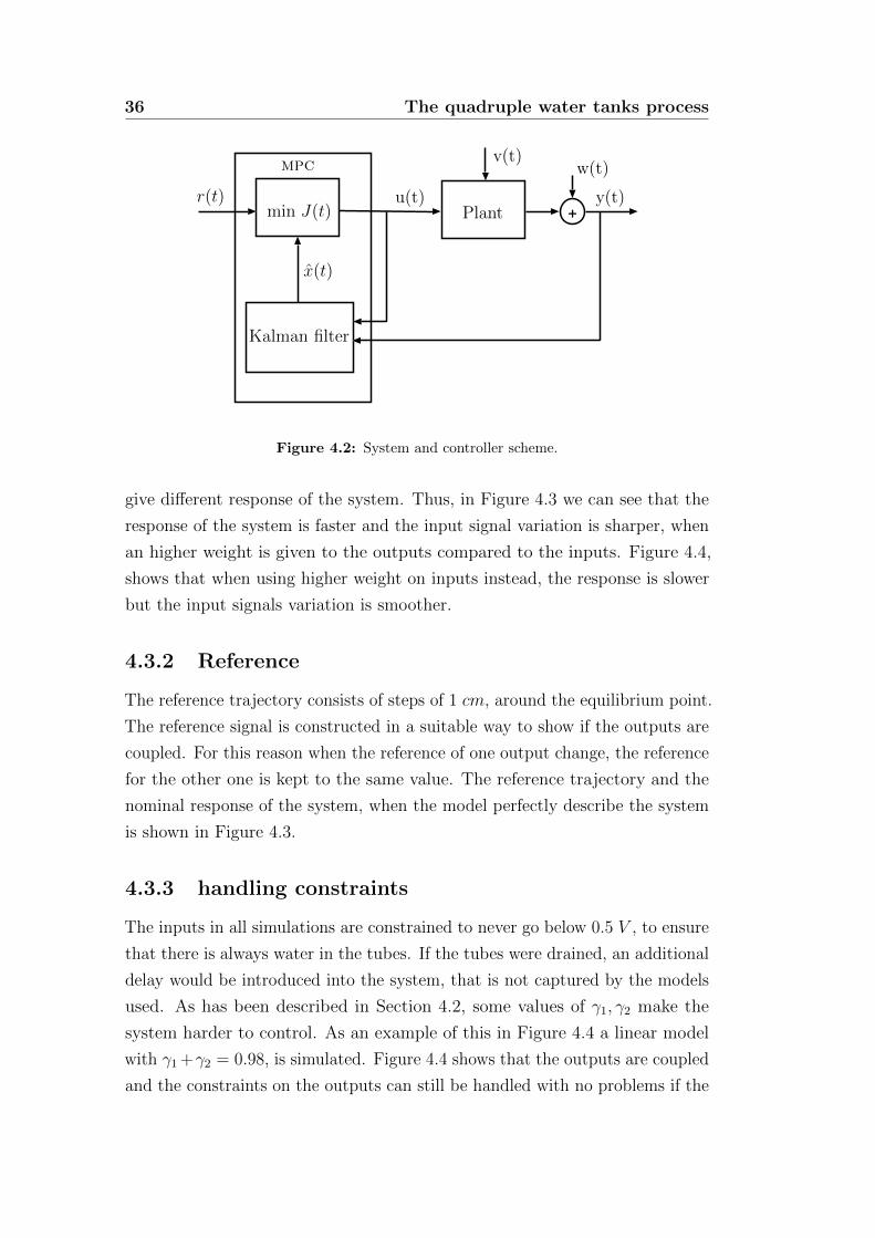
In Figure 4.2 the diagram block of the system is represented. The cost function
J(t) minimized by the MPC is on the form as in (2.4), v(t) and w(t) are process
and measurement noise respectively.
4.3.1 MPC weights
The weights, that we use to compute the cost function 2.4, are represented
by diagonal matrices with the following form: Qy = qyI and Qu = quI. That
is, both outputs and both inputs have respectively the same weights. The
weights qy and qu have been set manually. Different combinations of the weights
36 The quadruple water tanks process
+
x(t)
min J(t)r(t)
Plant
Kalman filter
u(t)
w(t)v(t)
y(t)
mpc
Figure 4.2: System and controller scheme.
give different response of the system. Thus, in Figure 4.3 we can see that the
response of the system is faster and the input signal variation is sharper, when
an higher weight is given to the outputs compared to the inputs. Figure 4.4,
shows that when using higher weight on inputs instead, the response is slower
but the input signals variation is smoother.
4.3.2 Reference
The reference trajectory consists of steps of 1 cm, around the equilibrium point.
The reference signal is constructed in a suitable way to show if the outputs are
coupled. For this reason when the reference of one output change, the reference
for the other one is kept to the same value. The reference trajectory and the
nominal response of the system, when the model perfectly describe the system
is shown in Figure 4.3.
4.3.3 handling constraints
The inputs in all simulations are constrained to never go below 0.5 V , to ensure
that there is always water in the tubes. If the tubes were drained, an additional
delay would be introduced into the system, that is not captured by the models
used. As has been described in Section 4.2, some values of γ1, γ2 make the
system harder to control. As an example of this in Figure 4.4 a linear model
with γ1 +γ2 = 0.98, is simulated. Figure 4.4 shows that the outputs are coupled
and the constraints on the outputs can still be handled with no problems if the

4.3 Water level control using MPC 37
0 10 20 30 40 50 60 70 8014
14.5
15
15.5
16
time [s]
water
tanklevels[cm]
Reference tracking
x1x2r1r2
0 10 20 30 40 50 60 70 800
2
4
6
8
10
time [s]
inputvoltage[V
]
Reference tracking
u1u2
Figure 4.3: Nominal response of a linear model, with γ1 + γ2 = 1.23, controlled with aMPC using exactly the same model. Inputs are constrained to never be below 0.5 V and
over 10 V . Outputs are constrained to be between 14 cm and 16 cm.
inputs are unconstrained. Figure 4.5 shows instead the response of the system
when the inputs are constrained to be between 0.5 V and 10 V .

38 The quadruple water tanks process
0 50 100 150 200 250 300 350 40014
14.5
15
15.5
16
time [s]
water
tanklevels[cm]
Reference tracking
x1x2r1r2
0 50 100 150 200 250 300 350 4000
5
10
time [s]
inputvoltage[V
]
Reference tracking
u1u2
Figure 4.4: Nominal response of a linear model, with γ1 + γ2 = 0.98 controlled with aMPC using exactly the same model. Inputs are unconstrained. Outputs are constrained to
be between 14 cm and 16 cm.

4.3 Water level control using MPC 39
0 50 100 150 200 250 300 350 40014
14.5
15
15.5
16
time [s]
water
tanklevels[cm]
Reference tracking
x1x2r1r2
0 50 100 150 200 250 300 350 4002
4
6
8
10
time [s]
inputvoltage[V
]
Reference tracking
u1u2
Figure 4.5: Nominal response of a linear model, with γ1 + γ2 = 0.98, controlled with aMPC using exactly the same model. Inputs are constrained to never be below 0.5 V and
over 10 V . Outputs are constrained to be between 14 cm and 16 cm.

40 The quadruple water tanks process
5Simulations
In this Chapter are presented the results of the simulations performed with
the quadruple water tank process described in Section 4.1. The results come
with a brief description leaving for Chapter 6 a more detailed analysis and
comparisons.
Nonlinear model
To perform simulations, we need to choose a model with fixed parameters
that represents the true system. In all the simulations the nonlinear model
(4.4) is considered to be the true system. The physical parameters of the
nonlinear model are described in Table 4.2. In all simulations the set of physical
parameters considered is described in Table 5.1. The estimated models, as
described in Section 3.2, have a fixed structure. The parameter vector θ, consists
of the physical parameters γ1 and γ2. The remaining physical parameters are
the one considered in Table 5.1. The physical parameters can be obtained for
example, with an initial long identification experiment.
The values of the sectional areas of tank’s outlets, are obtained from expressions
(4.6).
42 Simulations
Table 5.1: Physical parameters
Parameter Valuex0 [15, 15, 3, 12] cmu0 [7.8, 5.25] Vγ1 0.625γ2 0.625A 15.52 cm2
ai {0.17, 0.15, 0.11, 0.08} cm2
k1 4.14 cm3/(s·V)k2 4.14 cm3/(s·V)kc 1 V/cm
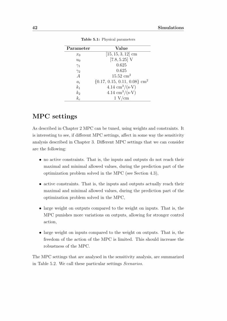
MPC settings
As described in Chapter 2 MPC can be tuned, using weights and constraints. It
is interesting to see, if different MPC settings, affect in some way the sensitivity
analysis described in Chapter 3. Different MPC settings that we can consider
are the following:
• no active constraints. That is, the inputs and outputs do not reach their
maximal and minimal allowed values, during the prediction part of the
optimization problem solved in the MPC (see Section 4.3),
• active constraints. That is, the inputs and outputs actually reach their
maximal and minimal allowed values, during the prediction part of the
optimization problem solved in the MPC,
• large weight on outputs compared to the weight on inputs. That is, the
MPC punishes more variations on outputs, allowing for stronger control
action,
• large weight on inputs compared to the weight on outputs. That is, the
freedom of the action of the MPC is limited. This should increase the
robustness of the MPC.
The MPC settings that are analysed in the sensitivity analysis, are summarized
in Table 5.2. We call these particular settings Scenarios.

43
Ny Nu qy qu ymin ymax umin umaxScenario 1 10 10 1 0.0001 0 cm 25 cm 0.5 V 15 VScenario 2 10 10 1 0.0001 14 cm 16 cm 0.5 V 10 VScenario 3 10 10 0.1 1 0 cm 25 cm 0.5 V 15 VScenario 4 10 10 0.1 1 14 cm 16 cm 0.5 V 10 V
Table 5.2: Scenarios.
Valve settings
As described in Section 4.2 depending on the value of γ1 + γ2, the system is
minimum phase or non-minimum phase. In particular when γ1 + γ2 is close to
1, the system is shifting from minimum phase to non-minimum phase. Thus,
it is interesting to compare the sensitivity analysis when the system is clearly
minimum phase (and clearly non minimum phase), to the sensitivity analysis
when the system is close to shifting between minimum phase and non-minimum
phase. This is performed for each scenario.
Procedure
1. First we choose the value of the true parameter.
2. An initial identification experiment with 1000 samples are performed. The
input used is a Gaussian white noise with covariance matrix Λu = 0.1I.
3. A reference tracking simulation of the initial estimated model is performed.
The parameter used in the MPC is the same used in the model. This
trajectory is then used to define the approximate application cost Vapp(θ),
see Section 3.2.
4. The Hessian of the approximate application cost, V′′app(θ, θ), is evaluated.
5. The Hessian is then used by the toolbox MOOSE to design the optimal
input spectrum that minimizes the input power. With the optimal input
spectrum the optimal input signal u∗ can be realized.
6. 100 identification experiments, using the optimal input u∗, are performed.
For each identification experiment 600 samples are used.

44 Simulations
7. 16 reference tracking simulations of the true system are performed. The
system is controlled by an MPC based on linear models, with param-
eter vectors randomly chosen from the ones obtained in the previous
identification experiments.
8. Step 6 is repeated, using a white Gaussian noise as input instead. The
variance is set to be equal to the one of the optimal input u∗.
9. Step 7 is repeated, using the estimates obtained in step 8.
5.1 Minimum phase setting: γ1 = γ2 = 0.625
With this setting the zeros of the system are s1 = −0.1040, s2 = −0.0160.
The simulation time is set to 400 s . The value of N used to calculate Vapp(θ, θ)
is equal to the simulation time.
5.1.1 Scenario 1
Reference tracking
Figure 5.1 shows the response of the linear model, with the initial parameter
estimate, controlled by an MPC using the same model. The response is fast and
due to the simulation time, it is difficult to distinguish the output signals from
the respective references. Figure 5.2 shows the input signals used to control
the system. Due to the little input weight, the input signal variations are big.
5.1 Minimum phase setting: γ1 = γ2 = 0.625 45
0 100 200 300 400
14
15
16
time [s]
water
tanklevels[cm]
Reference tracking
x1x2r1r2
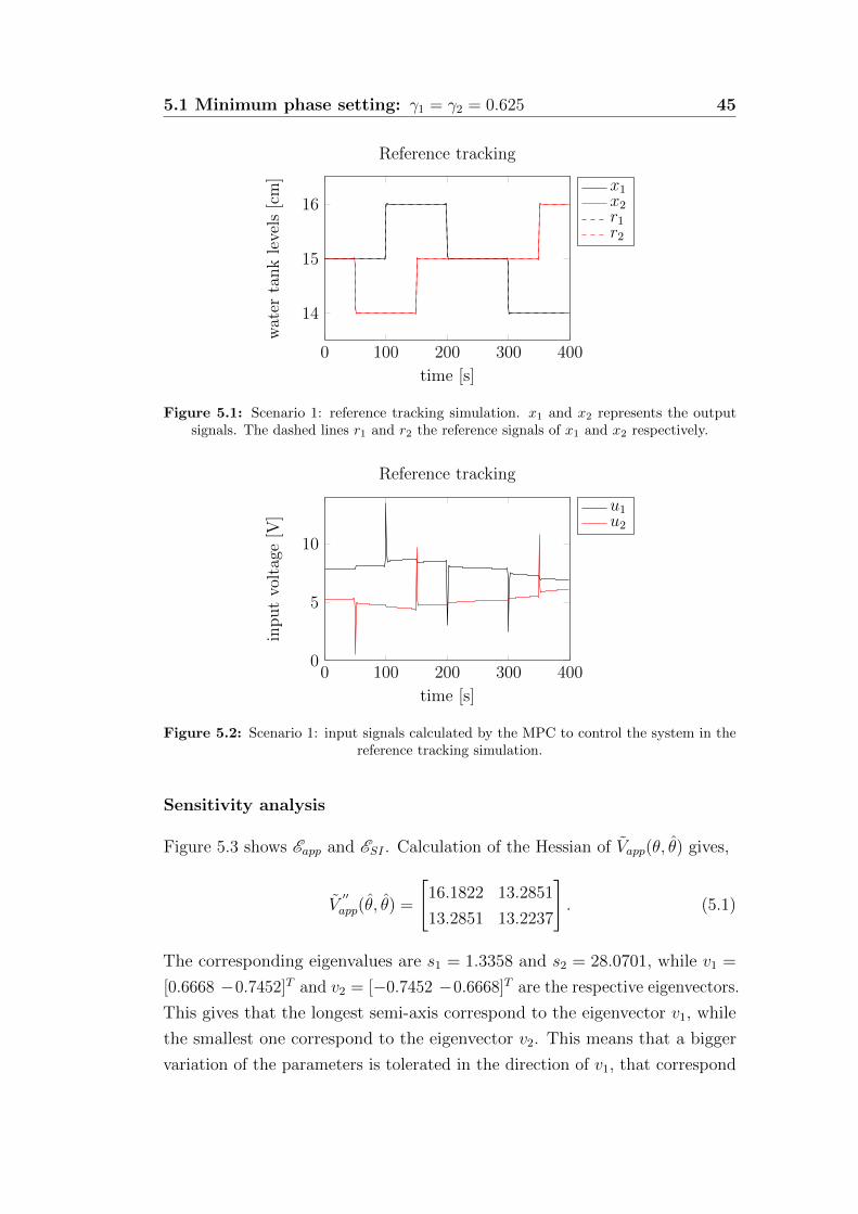
Figure 5.1: Scenario 1: reference tracking simulation. x1 and x2 represents the outputsignals. The dashed lines r1 and r2 the reference signals of x1 and x2 respectively.
0 100 200 300 4000
5
10
time [s]
inputvoltage[V
]
Reference tracking
u1u2
Figure 5.2: Scenario 1: input signals calculated by the MPC to control the system in thereference tracking simulation.
Sensitivity analysis
Figure 5.3 shows Eapp and ESI . Calculation of the Hessian of Vapp(θ, θ) gives,
V′′app(θ, θ) =
[16.1822 13.2851
13.2851 13.2237
]. (5.1)
The corresponding eigenvalues are s1 = 1.3358 and s2 = 28.0701, while v1 =
[0.6668 −0.7452]T and v2 = [−0.7452 −0.6668]T are the respective eigenvectors.
This gives that the longest semi-axis correspond to the eigenvector v1, while
the smallest one correspond to the eigenvector v2. This means that a bigger
variation of the parameters is tolerated in the direction of v1, that correspond

46 Simulations
to the straight line,
[θ1
θ2
]=
[θ1
0
θ20
]+ δ
[0.6668
−0.7452
]. (5.2)
The area of Eapp is 0.1633.
Figure 5.3 shows the resulting estimates from the 100 identification experiments,
using the optimal input. The estimates are spread around the true parameter,
following the shape of Eapp and 96% of these estimates lie inside the identification
ellipse. Figure 5.4 shows the reference tracking simulation of the true system,
0.55 0.6 0.65 0.7
0.55
0.6
0.65
0.7
θ1
θ 2
Figure 5.3: Scenario 1: results of step 6 of the procedure. 96% of the estimates lie insidethe identification ellipsoid.
see 4.4, controlled with an MPC based on linear models, that use the estimates
represented in Figure 5.3. Figure 5.5 shows the resulting estimates, from 100
0 50 100 150 200 250 300 350 400
14
15
16
time [s]
water
tanklevels[cm]
Reference tracking
x1x2r1r2
Figure 5.4: Scenario 1: results of step 7 of the procedure.
identification experiments, when a white Gaussian input with the same energy

5.1 Minimum phase setting: γ1 = γ2 = 0.625 47
of the optimal input is used. In this case only 13% of the estimates lie inside the
ellipse. Figure 5.6 shows the reference tracking simulation of the true system,
0.4 0.5 0.6 0.7 0.8
0.4
0.5
0.6
0.7
θ1
θ 2
Figure 5.5: Scenario 1: results of step 8 of the procedure. 13% of the estimates lie insidethe identification ellipsoid.
see 4.4, controlled with an MPC based on linear models, that use the estimates
represented in Figure 5.5.
0 50 100 150 200 250 300 350 40010
12
14
16
18
20
time [s]
water
tanklevels[cm]
Reference tracking
x1x2r1r2
Figure 5.6: Scenario 1: results of step 9 of the procedure.
Observation 1
This example demonstrate that using the optimal input signal in the identifi-
cation experiments, give an higher percentage of estimates that lie inside the
application ellipsoid, compared to the number of estimates inside the appli-
cation ellipsoid that we obtain when a white Gaussian noise with the same
energy is used.

48 Simulations
5.1.2 Scenario 2
0 100 200 300 40014
14.5
15
15.5
16
time [s]
water
tanklevels[cm]
Reference tracking
x1x2r1r2
Figure 5.7: Scenario 2: reference tracking simulation. x1 and x2 represents the outputsignals. The dashed lines r1 and r2 the reference signals of x1 and x2 respectively.
0 100 200 300 4000
2
4
6
8
10
time [s]
inputvoltage[V
]
Reference tracking
u1u2
Figure 5.8: Scenario 2: input signals calculated by the MPC to control the system in thereference tracking simulation.
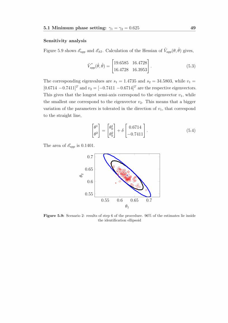
5.1 Minimum phase setting: γ1 = γ2 = 0.625 49
Sensitivity analysis
Figure 5.9 shows Eapp and ESI . Calculation of the Hessian of Vapp(θ, θ) gives,
V′′app(θ, θ) =
[19.6585 16.4728
16.4728 16.3953
]. (5.3)
The corresponding eigenvalues are s1 = 1.4735 and s2 = 34.5803, while v1 =
[0.6714 −0.7411]T and v2 = [−0.7411 −0.6714]T are the respective eigenvectors.
This gives that the longest semi-axis correspond to the eigenvector v1, while
the smallest one correspond to the eigenvector v2. This means that a bigger
variation of the parameters is tolerated in the direction of v1, that correspond
to the straight line,
[θ1
θ2
]=
[θ1
0
θ20
]+ δ
[0.6714
−0.7411
]. (5.4)
The area of Eapp is 0.1401.
0.55 0.6 0.65 0.7
0.55
0.6
0.65
0.7
θ1
θ 2
Figure 5.9: Scenario 2: results of step 6 of the procedure. 96% of the estimates lie insidethe identification ellipsoid

50 Simulations
0 50 100 150 200 250 300 350 400
14
15
16
time [s]
water
tanklevels[cm]
Reference tracking
x1x2r1r2
Figure 5.10: Scenario 2: results of step 7 of the procedure.
Observation 2
In Figure 5.11 can be noticed that some parameters, identified using the white
Gaussian noise, can make the system instable (we underline that the parameter
used in step 9 of the procedure described, are chosen randomly from all the
estimates obtained in step 8).

5.1 Minimum phase setting: γ1 = γ2 = 0.625 51
0.4 0.5 0.6 0.7
0.5
0.6
0.7
θ1
θ 2
0 50 100 150 200 250 300 350 400−50
0
50
100
time [s]
water
tanklevels[cm]
Reference tracking
x1x2r1r2
Figure 5.11: Scenario 2: results of step 8 (in the upper figure), and step 9 (in the lowerfigure)

52 Simulations
5.1.3 Scenario 3
0 100 200 300 400
14
15
16
time [s]
water
tanklevels[cm]
Reference tracking
x1x2r1r2
Figure 5.12: Scenario 3: reference tracking simulation. x1 and x2 represents the outputsignals. The dashed lines r1 and r2 the reference signals of x1 and x2 respectively.
0 100 200 300 4004
6
8
time [s]
inputvoltage[V
]
Reference tracking
u1u2
Figure 5.13: Scenario 3: input signals calculated by the MPC to control the system in thereference tracking simulation.

5.1 Minimum phase setting: γ1 = γ2 = 0.625 53
Sensitivity analysis
Figure 5.15 shows Eapp and ESI . Calculation of the Hessian of Vapp(θ, θ) gives,
V′′app(θ, θ) =
[15.1718 12.5269
12.5269 12.4377
]. (5.5)
The corresponding eigenvalues are s1 = 1.2035 and s2 = 26.4060, while v1 =
[0.6677 −0.7445]T and v2 = [−0.7445 −0.6677]T are the respective eigenvectors.
This gives that the longest semi-axis correspond to the eigenvector v1, while
the smallest one correspond to the eigenvector v2. This means that a bigger
variation of the parameters is tolerated in the direction of v1, that correspond
to the straight line,
[θ1
θ2
]=
[θ1
0
θ20
]+ δ
[0.6677
−0.7445
]. (5.6)
The area of Eapp is 0.1774.
0.55 0.6 0.65 0.7
0.55
0.6
0.65
0.7
θ1
θ 2
Figure 5.14: Scenario 3: results of step 6 of the procedure. 92% of the estimates lie insidethe identification ellipsoid
54 Simulations
0 50 100 150 200 250 300 350 400
14
15
16
time [s]
water
tanklevels[cm]
Reference tracking
x1x2r1r2
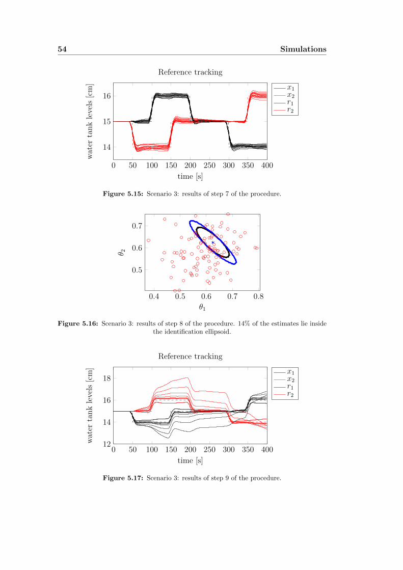
Figure 5.15: Scenario 3: results of step 7 of the procedure.
0.4 0.5 0.6 0.7 0.8
0.5
0.6
0.7
θ1
θ 2
Figure 5.16: Scenario 3: results of step 8 of the procedure. 14% of the estimates lie insidethe identification ellipsoid.
0 50 100 150 200 250 300 350 40012
14
16
18
time [s]
water
tanklevels[cm]
Reference tracking
x1x2r1r2
Figure 5.17: Scenario 3: results of step 9 of the procedure.

5.1 Minimum phase setting: γ1 = γ2 = 0.625 55
0 100 200 300 40014
14.5
15
15.5
16
time [s]
water
tanklevels[cm]
Reference tracking
x1x2r1r2
Figure 5.18: Scenario 4: reference tracking simulation. x1 and x2 represents the outputsignals. The dashed lines r1 and r2 the reference signals of x1 and x2 respectively.
0 100 200 300 4004
6
8
time [s]
inputvoltage[V
]
Reference tracking
u1u2
Figure 5.19: Scenario 4: input signals calculated by the MPC to control the system in thereference tracking simulation.
5.1.4 Scenario 4
Sensitivity analysis
Figure 5.21 shows Eapp and ESI . Calculation of the Hessian of Vapp(θ, θ) gives,
V′′app(θ, θ) =
[17.0033 14.1985
14.1985 14.0111
]. (5.7)
The corresponding eigenvalues are s1 = 1.2301 and s2 = 29.7843, while v1 =
[0.6690 −0.7432]T and v2 = [−0.7432 −0.6690]T are the respective eigenvectors.
This gives that the longest semi-axis correspond to the eigenvector v1, while
the smallest one correspond to the eigenvector v2. This means that a bigger

56 Simulations
variation of the parameters is tolerated in the direction of v1, that correspond
to the straight line,
[θ1
θ2
]=
[θ1
0
θ20
]+ δ
[0.6690
−0.7432
]. (5.8)
The area of Eapp is 0.1652.
0.55 0.6 0.65 0.7
0.55
0.6
0.65
0.7
θ1
θ 2
Figure 5.20: Scenario 4: results of step 6 of the procedure. 96% of the estimates lie insidethe identification ellipsoid
0 50 100 150 200 250 300 350 400
14
15
16
time [s]
water
tanklevels[cm]
Reference tracking
x1x2r1r2
Figure 5.21: Scenario 4: results of step 7 of the procedure.

5.1 Minimum phase setting: γ1 = γ2 = 0.625 57
0.5 0.6 0.7 0.8
0.5
0.6
0.7
θ1
θ 2
Figure 5.22: Scenario 4: results of step 8 of the procedure. 17% of the estimates lie insidethe identification ellipsoid.
0 50 100 150 200 250 300 350 40013
14
15
16
17
time [s]
water
tanklevels[cm]
Reference tracking
x1x2r1r2
Figure 5.23: Scenario 4: results of step 9 of the procedure.
58 Simulations
5.2 Minimum phase setting: γ1 = γ2 = 0.505
With this setting the zeros of the system are: s1 = −0.1572, s2 = −0.0012
5.2.1 Scenario 1
Reference tracking
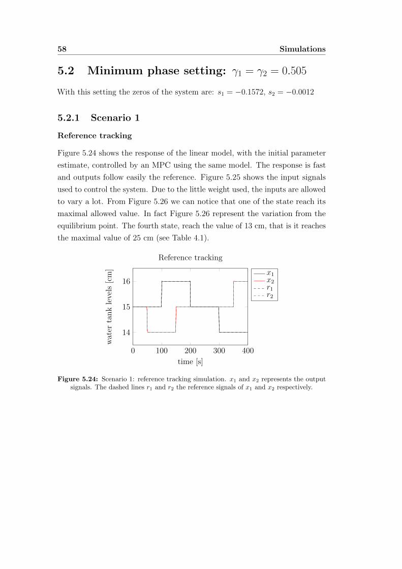
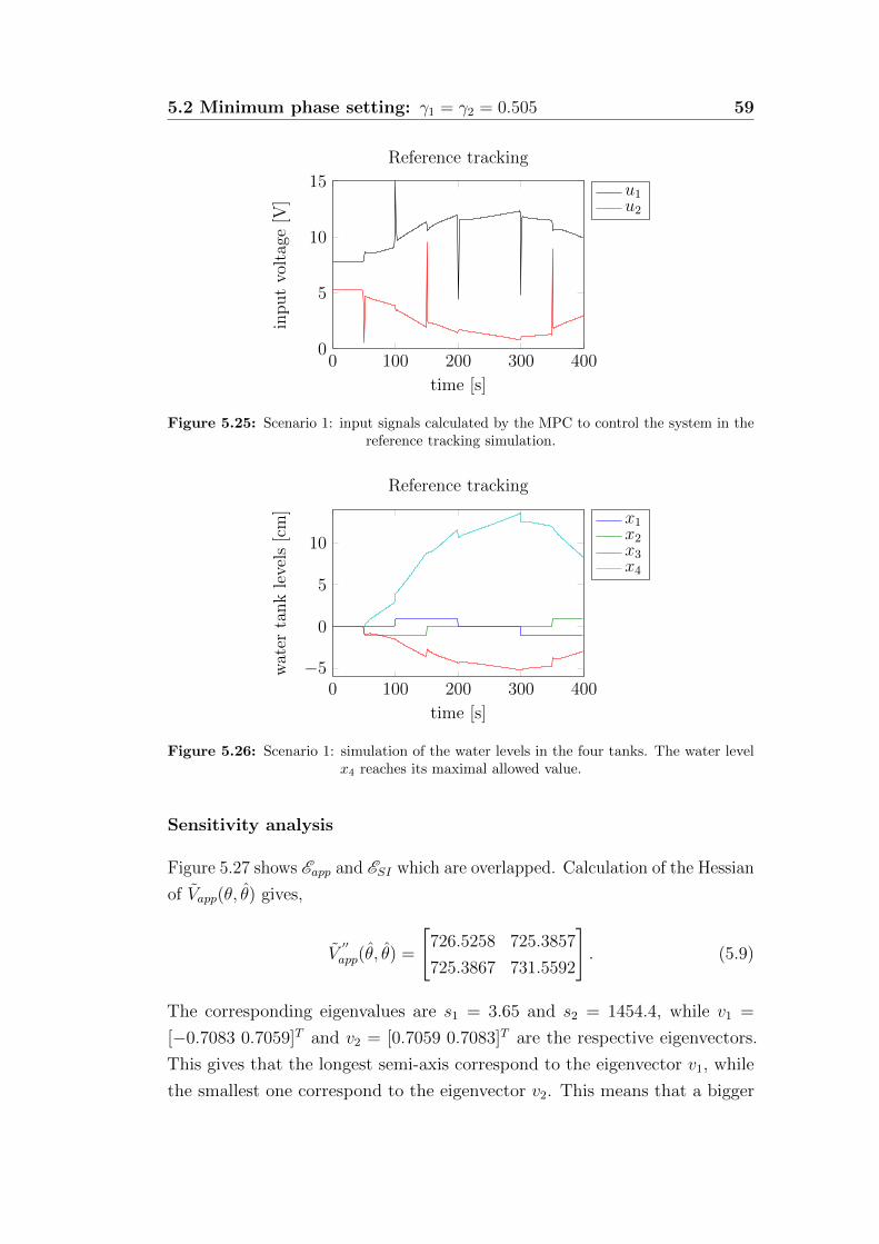
Figure 5.24 shows the response of the linear model, with the initial parameter
estimate, controlled by an MPC using the same model. The response is fast
and outputs follow easily the reference. Figure 5.25 shows the input signals
used to control the system. Due to the little weight used, the inputs are allowed
to vary a lot. From Figure 5.26 we can notice that one of the state reach its
maximal allowed value. In fact Figure 5.26 represent the variation from the
equilibrium point. The fourth state, reach the value of 13 cm, that is it reaches
the maximal value of 25 cm (see Table 4.1).
0 100 200 300 400
14
15
16
time [s]
water
tanklevels[cm]
Reference tracking
x1x2r1r2
Figure 5.24: Scenario 1: reference tracking simulation. x1 and x2 represents the outputsignals. The dashed lines r1 and r2 the reference signals of x1 and x2 respectively.
5.2 Minimum phase setting: γ1 = γ2 = 0.505 59
0 100 200 300 4000
5
10
15
time [s]
inputvoltage[V
]
Reference tracking
u1u2
Figure 5.25: Scenario 1: input signals calculated by the MPC to control the system in thereference tracking simulation.
0 100 200 300 400−5
0
5
10
time [s]
water
tanklevels[cm]
Reference tracking
x1x2x3x4
Figure 5.26: Scenario 1: simulation of the water levels in the four tanks. The water levelx4 reaches its maximal allowed value.
Sensitivity analysis
Figure 5.27 shows Eapp and ESI which are overlapped. Calculation of the Hessian
of Vapp(θ, θ) gives,
V′′app(θ, θ) =
[726.5258 725.3857
725.3867 731.5592
]. (5.9)
The corresponding eigenvalues are s1 = 3.65 and s2 = 1454.4, while v1 =
[−0.7083 0.7059]T and v2 = [0.7059 0.7083]T are the respective eigenvectors.
This gives that the longest semi-axis correspond to the eigenvector v1, while
the smallest one correspond to the eigenvector v2. This means that a bigger

60 Simulations
variation of the parameters is tolerated in the direction of v1, that correspond
to the straight line,
[θ1
θ2
]=
[θ1
0
θ20
]+ δ
[−0.7083
0.7059
]. (5.10)
The area of Eapp is 0.0137.
0.44 0.46 0.48 0.5 0.52 0.54 0.56
0.46
0.48
0.5
0.52
0.54
θ1
θ 2
Figure 5.27: Scenario 1: results of step 6 of the procedure. 11% of the estimates lie insidethe identification ellipsoid.
0 50 100 150 200 250 300 350 400
14
15
16
time [s]
water
tanklevels[cm]
Reference tracking
x1x2r1r2
Figure 5.28: Scenario 1: results of step 7 of the procedure.

5.2 Minimum phase setting: γ1 = γ2 = 0.505 61
0.44 0.46 0.48 0.5 0.52 0.54
0.46
0.48
0.5
0.52
0.54
θ1
θ 2
Figure 5.29: Scenario 1: results of step 8 of the procedure. 1% of the estimates lie insidethe identification ellipsoid.
0 50 100 150 200 250 300 350 400
12
14
16
18
time [s]
water
tanklevels[cm]
Reference tracking
x1x2r1r2
Figure 5.30: Scenario 1: results of step 9 of the procedure.
Observation 3
Figure 5.27 shows that when the sum of γ is close to 1 the application ellipsoid
stretch out in the direction of the longer semi-axes more than in the other
cases.
Observation 4: offset in the estimates
Figures 5.27,5.33,5.38 and 5.43 show that the estimates make a blob that is
not centered around the true parameter θ0. It is interesting to notice that this
behavior was already present in the minimum phase case, just not so evident.
See for example figures 5.9, 5.15. This behavior is discussed more in detail in
Chapter 6.

62 Simulations
5.2.2 Scenario 2
0 100 200 300 40014
14.5
15
15.5
16
time [s]
water
tanklevels[cm]
Reference tracking
x1x2r1r2
Figure 5.31: Scenario 2: reference tracking simulation. x1 and x2 represents the outputsignals. The dashed lines r1 and r2 the reference signals of x1 and x2 respectively.
0 100 200 300 4000
5
10
15
time [s]
inputvoltage[V
]
Reference tracking
u1u2
Figure 5.32: Scenario 2: input signals calculated by the MPC to control the system in thereference tracking simulation.
Sensitivity analysis
Figure 5.33 shows Eapp and ESI . Calculation of the Hessian of Vapp(θ, θ) gives,
V′′app(θ, θ) =
[762.3064 761.0394
761.0394 767.1592
]. (5.11)
The corresponding eigenvalues are s1 = 3.68 and s2 = 1525.8, while v1 =
[−0.7082 0.7060]T and v2 = [0.7060 0.7082]T are the respective eigenvectors.

5.2 Minimum phase setting: γ1 = γ2 = 0.505 63
This gives that the longest semi-axis correspond to the eigenvector v1, while
the smallest one correspond to the eigenvector v2. This means that a bigger
variation of the parameters is tolerated in the direction of v1, that correspond
to the straight line,
[θ1
θ2
]=
[θ1
0
θ20
]+ δ
[−0.7082
0.7060
]. (5.12)
The area of Eapp is 0.0133.
0.44 0.46 0.48 0.5 0.52 0.54 0.56
0.46
0.48
0.5
0.52
0.54
θ1
θ 2
Figure 5.33: Scenario 2: results of step 6 of the procedure. No estimates lie inside theidentification ellipsoid.
0 50 100 150 200 250 300 350 400
14
15
16
time [s]
water
tanklevels[cm]
Reference tracking
x1x2r1r2
Figure 5.34: Scenario 2: results of step 7 of the procedure.
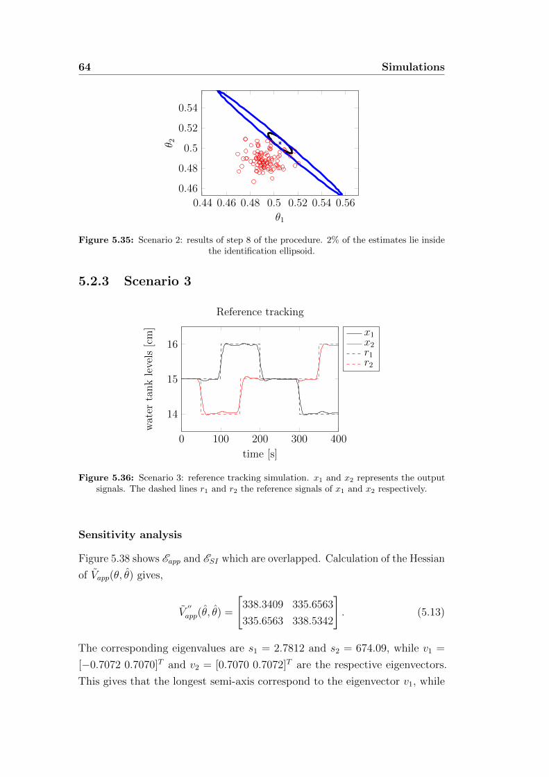
64 Simulations
0.44 0.46 0.48 0.5 0.52 0.54 0.56
0.46
0.48
0.5
0.52
0.54
θ1
θ 2
Figure 5.35: Scenario 2: results of step 8 of the procedure. 2% of the estimates lie insidethe identification ellipsoid.
5.2.3 Scenario 3
0 100 200 300 400
14
15
16
time [s]
water
tanklevels[cm]
Reference tracking
x1x2r1r2
Figure 5.36: Scenario 3: reference tracking simulation. x1 and x2 represents the outputsignals. The dashed lines r1 and r2 the reference signals of x1 and x2 respectively.
Sensitivity analysis
Figure 5.38 shows Eapp and ESI which are overlapped. Calculation of the Hessian
of Vapp(θ, θ) gives,
V′′app(θ, θ) =
[338.3409 335.6563
335.6563 338.5342
]. (5.13)
The corresponding eigenvalues are s1 = 2.7812 and s2 = 674.09, while v1 =
[−0.7072 0.7070]T and v2 = [0.7070 0.7072]T are the respective eigenvectors.
This gives that the longest semi-axis correspond to the eigenvector v1, while
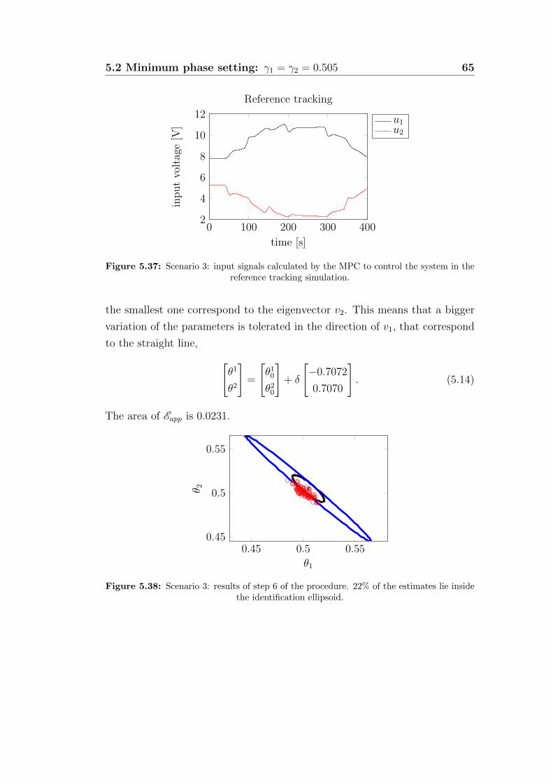
5.2 Minimum phase setting: γ1 = γ2 = 0.505 65
0 100 200 300 4002
4
6
8
10
12
time [s]
inputvoltage[V
]
Reference tracking
u1u2
Figure 5.37: Scenario 3: input signals calculated by the MPC to control the system in thereference tracking simulation.
the smallest one correspond to the eigenvector v2. This means that a bigger
variation of the parameters is tolerated in the direction of v1, that correspond
to the straight line,
[θ1
θ2
]=
[θ1
0
θ20
]+ δ
[−0.7072
0.7070
]. (5.14)
The area of Eapp is 0.0231.
0.45 0.5 0.550.45
0.5
0.55
θ1
θ 2
Figure 5.38: Scenario 3: results of step 6 of the procedure. 22% of the estimates lie insidethe identification ellipsoid.

66 Simulations
0 50 100 150 200 250 300 350 400
14
15
16
time [s]
water
tanklevels[cm]
Reference tracking
x1x2r1r2
Figure 5.39: Scenario 3: results of step 7 of the procedure.
0.45 0.5 0.550.45
0.5
0.55
θ1
θ 2
Figure 5.40: Scenario 3, check of theory - u∗.
5.2.4 Scenario 4
Sensitivity analysis
Figure 5.43 shows Eapp and ESI . Calculation of the Hessian of Vapp(θ, θ) gives,
V′′app(θ, θ) =
[640.14 638.5481
638.5481 642.8231
]. (5.15)
The corresponding eigenvalues are s1 = 2.932 and s2 = 1280, while v1 =
[−0.7078 0.7064]T and v2 = [0.7064 0.7078]T are the respective eigenvectors.
This gives that the longest semi-axis correspond to the eigenvector v1, while
the smallest one correspond to the eigenvector v2. This means that a bigger
variation of the parameters is tolerated in the direction of v1, that correspond

5.2 Minimum phase setting: γ1 = γ2 = 0.505 67
0 100 200 300 40014
14.5
15
15.5
16
time [s]
water
tanklevels[cm]
Reference tracking
x1x2r1r2
Figure 5.41: Scenario 4: reference tracking simulation. x1 and x2 represents the outputsignals. The dashed lines r1 and r2 the reference signals of x1 and x2 respectively.
0 100 200 300 4000
5
10
time [s]
inputvoltage[V
]
Reference tracking
u1u2
Figure 5.42: Scenario 4: input signals calculated by the MPC to control the system in thereference tracking simulation.
to the straight line,
[θ1
θ2
]=
[θ1
0
θ20
]+ δ
[−0.7078
0.7064
]. (5.16)
The area of Eapp is 0.0163.

68 Simulations
0.45 0.5 0.550.45
0.5
0.55
θ1
θ 2
Figure 5.43: Scenario 4: results of step 6 of the procedure. No estimates lie inside theidentification ellipsoid.
0.45 0.5 0.550.45
0.5
0.55
θ1
θ 2
Figure 5.44: Scenario 4: results of step 8 of the procedure. No estimates lie inside theidentification ellipsoid.
5.3 Non minimum phase case: γ1 = γ2 = 0.25
With this setting the zeros of the system are: s1 = −0.4449, s2 = 0.2047. For
this case we do not show any figures of the results because could be repetitive
and not much interesting. All the results of this setting are used instead to
make comparisons in Chapter 6.
5.3.1 Observation
For this setting, the reference tracking was quite hard when the constraints on
inputs were applied. So for this setting Scenario 2 and 4 are simulated with
only output constraints.

6Discussion
The numerical results obtained from the simulations presented in Chapter 5
are summarized in Table 6.1,6.2,6.3. From the analysis of the obtained results
it is possible to make the following observations:
1. The area of the application ellipsoid is smaller when γ1 +γ2 ≈ 1. Meaning
that this setting is actually harder to control, in the sense that the
requirements on the model are much higher. See for example Figure 6.2.
2. The eigenvalue s2 becomes very high when γ1 + γ2 ≈ 1, namely, the
semi-axis in the direction of v2 becomes very small. That is, Eapp becomes
much narrower in the direction of v2. This means that performance
degrades mostly when estimated parameters vary in that direction.
3. The area of the application ellipsoid is bigger when we use higher weights
on inputs compared to outputs. Meaning that this setting results in a
larger number of models that meet the performance specifications. Thus,
the robustness of the controller is higher.
4. The longer semi-axis corresponds to the direction of the eigenvector v1,

70 Discussion
while the smallest one corresponds to the eigenvector v2. This means that
a bigger variation of the estimates in the direction of the eigenvector v1
is tolerated.
5. Parameter variations in the direction of v2 give the higher degradation
of performance. From Table 6.2 we can see that, when γ1 + γ2 ≈ 1, that
direction is defined by the line y = x+ (γ1 + γ2).
6. The area of the application ellipsoid is usually smaller when we analyse
scenarios with active constraints compared to the area obtained with
scenarios with no active constraints. See for example Figure 6.3.
Scenario 1 Scenario 2 Scenario 3 Scenario 4Area 0.1633 0.1401 0.1774 0.1652s1 1.358 1.4735 1.2035 1.2301s2 28.07 34.58 26.406 29.7843
v1
[0.668−0.7452
] [0.6714−0.7411
] [0.6677−0.7432
] [0.669−0.7432
]
v2
[−0.7452−0.668
] [−0.7411−0.6714
] [−0.7432−0.6677
] [−0.7432−0.669
]
Table 6.1: γ1 = γ2 = 0.625
Scenario 1 Scenario 2 Scenario 3 Scenario 4Area 0.0137 0.0133 0.0231 0.0163s1 3.650 3.6800 2.7812 2.932s2 1454.4 1525.8 674.09 1280
v1
[0.7083−0.7059
] [0.7082−0.7060
] [0.7072−0.7070
] [0.7078−0.7064
]
v2
[−0.7059−0.7083
] [−0.7060−0.7082
] [−0.7070−0.7072
] [−0.7064−0.7078
]
Table 6.2: γ1 = γ2 = 0.505
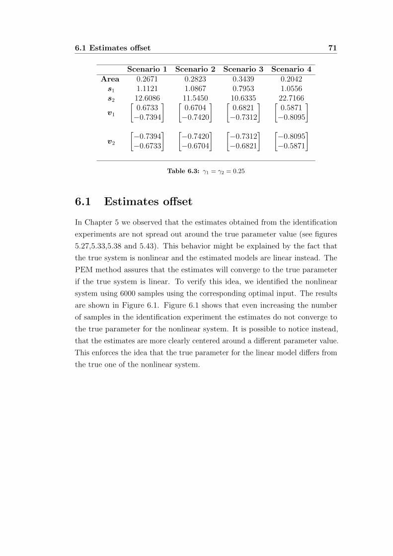
6.1 Estimates offset 71
Scenario 1 Scenario 2 Scenario 3 Scenario 4Area 0.2671 0.2823 0.3439 0.2042s1 1.1121 1.0867 0.7953 1.0556s2 12.6086 11.5450 10.6335 22.7166
v1
[0.6733−0.7394
] [0.6704−0.7420
] [0.6821−0.7312
] [0.5871−0.8095
]
v2
[−0.7394−0.6733
] [−0.7420−0.6704
] [−0.7312−0.6821
] [−0.8095−0.5871
]
Table 6.3: γ1 = γ2 = 0.25
6.1 Estimates offset
In Chapter 5 we observed that the estimates obtained from the identification
experiments are not spread out around the true parameter value (see figures
5.27,5.33,5.38 and 5.43). This behavior might be explained by the fact that
the true system is nonlinear and the estimated models are linear instead. The
PEM method assures that the estimates will converge to the true parameter
if the true system is linear. To verify this idea, we identified the nonlinear
system using 6000 samples using the corresponding optimal input. The results
are shown in Figure 6.1. Figure 6.1 shows that even increasing the number
of samples in the identification experiment the estimates do not converge to
the true parameter for the nonlinear system. It is possible to notice instead,
that the estimates are more clearly centered around a different parameter value.
This enforces the idea that the true parameter for the linear model differs from
the true one of the nonlinear system.

72 Discussion
0.45 0.5 0.550.45
0.5
0.55
θ1
θ 2
0.45 0.5 0.550.45
0.5
0.55
θ1
θ 2
Figure 6.1: Comparison that show the estimates offset when 600 samples (left figure) andwhen 6000 samples (right figure) are used in the system identification experiment.
0.1 0.2 0.3 0.4 0.5 0.6 0.70.1
0.2
0.3
0.4
0.5
0.6
0.7
Figure 6.2: Comparison of the application ellipses obtained for different values of the trueparameter vector. The application ellipse becomes very small when γ1 + γ2 ≈ 1. The rectsrepresent the straight line y = −x+ (γ1 + γ2) for the respective value of γ1, γ2. The rects
help to see the orientation of the ellipse in the parameter space.

6.1 Estimates offset 73
0.5 0.55 0.6 0.65 0.7 0.750.5
0.55
0.6
0.65
0.7
0.75
Figure 6.3: Comparison between the application ellipse obtained from scenario 1 (innerellipse) and the application ellipse obtained from scenario 3 (outer ellipse). With scenario 3(higher weight on inputs), the ellipse’s area is bigger. The center of the ellipses is the true
parameter vector.

74 Discussion

7Conclusions and future work
In this chapter we make some remarks of the obtained results and suggest some
ideas for future work.
The main objective of this master thesis work was to investigate if MPC settings
affect the shape and the important directions of the application ellipsoid Eapp.
The quadruple water tank process has the characteristic property of changing
the position of one zero, to be minimum phase or non minimum phase, using the
physical parameters γ1, γ2 (see Section 4.2). Hence, MPC tuning parameters
and constraints are used to define four scenarios. Simulations are carried out
for every scenario considering the system to be minimum phase, non minimum
phase and close to shifting from minimum phase to non minimum phase. The
latter case corresponds to when one system’s zero is close to the origin, that
is γ1 + γ2 ≈ 1. This situation was really hard to control so constraints on
input were not imposed. Obtained results are summarized with the following
remarks:
• Different MPC settings affect the area of the application ellipsoid. When
we consider higher weights on inputs the area of Eapp becomes bigger. This
means that limiting the freedom of the controller requires less accurate
models. Active constraints increase controller’s performance demand and

76 Conclusions and future work
reduce the robustness of the controller resulting in a smaller application
ellipsoid’s area.
• Different positions of the system’s zero have a strong influence on Eapp.
The closer the zero is to the origin, the narrower becomes the Eapp in the
smaller semi-axis direction. The position of the system’s zero depends on
the value assumed by γ1 + γ2.
Future work
This master thesis project does not represent a complete solution and further
researches are recommended in the following areas:
• The number of parameters: our analysis takes only two parameters, γ1
and γ2, into account. In this case Eapp has only 2 dimensions and it can
be graphically represented. Furthermore, the two parameters we consider
have a straightforward physical interpretation. For the future work we
suggest to take into consideration all the parameters of the nonlinear
model of the water tanks.
• Application cost: in this work we consider performance degradation in
reference tracking applications. Another possibility is to focus on the
disturbance rejection. A different application cost for this application
should be defined.
• Real plant: we suggest to verify the obtained results of the simulations
on the real water tank process.
Bibliography
[1] Sciencedirect.
[2] Marta Barenthin Syberg. Complexity Issues, Validation and Input Design
for Control in System Identification. PhD thesis, KTH, Automatic Control,
2008. QC 20100702.
[3] Stephen Boyd and Lieven Vandenberghe. Convex Optimization. CUP,
2004.
[4] M. Annergren C. A. Larsson. Moose: Model based optimal input design
toolbox for matlab, 2011.
[5] Torkel Glad and Lennart Ljung. Control Theory : Multivariable & Non-
linear Methods. CRC, March 2000.
[6] M. Grant and S. Boyd. Graph implementations for nonsmooth con-
vex programs. In V. Blondel, S. Boyd, and H. Kimura, editors, Recent
Advances in Learning and Control, Lecture Notes in Control and Infor-
mation Sciences, pages 95–110. Springer-Verlag Limited, 2008. http:
//stanford.edu/~boyd/graph_dcp.html.
[7] M. Grant and S. Boyd. CVX: Matlab software for disciplined convex
programming, version 1.21. ../../cvx, apr 2011.
[8] Hakan Hjalmarsson. System identification of complex and structured sys-
tems. European Journal of Control, 15(3-4):275–310, 2009. QC 20110112.
[9] Henrik Jansson and Hakan Hjalmarsson. Input design via lmis admitting
frequency-wise model specifications in confidence regions. IEEE Transac-
tions on Automatic Control, 50(10):1534–1549, 2005. QC 20100525.

78 Bibliography
[10] Karl H. Johansson and J. L. R. Nunes. A multivariable laboratory process
with an adjustable zero. In Proceedings of the American Control Conference,
Philadelphia, Pennsylvania June 1998, pages 2045–2049. AACC, 1998. QC
20120227.
[11] Karl Henrik Johansson. The quadruple-tank process-a multivariable lab-
oratory process with an adjustable zero. IEEE Transactions on Control
Systems Technology, 8(3):456–465, 2000. QC 20120227.
[12] Christian Larsson. Toward applications oriented optimal input design with
focus on model predictive control, 2011. QC 20111013.
[13] Christian A. Larsson, Mariette Annergren, and Hakan Hjalmarsson. On
optimal input design in system identification for model predictive control.
In CDC-ECE, pages 805–810. IEEE, 2011.
[14] Christian A. Larsson, Cristian R. Rojas, and Hakan Hjalmarsson. MPC
oriented experiment design. In Proceedings of the 18th IFAC World
Congress, pages 9966–9971, 2011. QC 20111122.
[15] Lennart Ljung. System Identification: Theory for the User. Prentice-Hall,
Upper Saddle River, New Jersey, 2nd edition, 1999.
[16] Jan Marian Maciejowski. Predictive control: with constraints. Prentice-
Hall, pub-PH:adr, 2002.
[17] G. Picci. Metodi statistici per l’identificazione di sistemi lineari, 2011.
[18] Bo Wahlberg, Hakan Hjalmarsson, and Mariette Annergren. On optimal
input design in system identification for control. In 49TH IEEE CON-
FERENCE ON DECISION AND CONTROL (CDC), pages 5548–5553.
IEEE, 2010.
[19] Bo Wahlberg, Hakan Hjalmarsson, and Mariette Annergren. On optimal
input design in system identification for control. In CDC, pages 5548–5553.
IEEE, 2010.
[20] Wikipedia. Plagiarism — Wikipedia, the free encyclopedia, 2004. [Online;
accessed 22-July-2004].

Bibliography 79
[21] Yucai Zhu. System identification for process control: recent experience and
outlook. International Journal of Modelling, Identification and Control, 6,
2009.