APPLICATIONS OF VARIATIONAL METHODS - …user.engineering.uiowa.edu/~kkchoi/Chapter_11.pdf · 11 APPLICATIONS OF VARIATIONAL METHODS In order to illustrate the variational theory

11

APPLICATIONS OF VARIATIONAL METHODS

In order to illustrate the variational theory developed in Chapter 10, a number of applications are studied in this chapter. The examples, which are of interest in themselves, illustrate the complexity encountered in general problems that precludes closed form solutions. Concrete applications of physical significance also show that the power of variational methods rests on careful verification of hypotheses that underlie the methods.

11.1 BOUNDARY-VALUE PROBLEMS FOR ORDINARY DIFFERENTIAL EQUATIONS

Many problems in mechanics reduce to finding the solution of an ordinary differential equation that satisfies homogeneous boundary conditions. The Ritz method of Chapter 10 can be applied to such problems, if it can be established that the associated operator is symmetric and positive definite, or even better positive bounded below.

Theoretical Results

Consider frrst the ordinary differential equation

d ( du) Au = - dX p(x) dx + q(x) u = f(x)

A solution is sought in C1(a, b) that satisfies the boundary conditions

ex u'(a) - ~ u(a) = 0

y u'(b) + 8 u(b) = 0

(11.1.1)

(11.1.2)

where ex, ~. y, and 8 are constants. The following assumptions are made regarding the functions p(x) and q(x) and constants ex, ~. y, and 8:

498

(a) p(x), p'(x), and q(x) are continuous in a ~ x ~ b. (b) p(x) ~ 0, q(x) ~ 0. (c) the function p(x) can vanish at a number of points in a ~ x ~ b, but the integral

Sec. 11.1 Boundary-Value Problems for Ordinary Differential Equations

Jb dx F- -

- a p(x)

499

has finite value. In particular, this requirement is satisfied if p(x) ~ k > 0 in a~x ~b.

(d) the constants a,~. y, and o are non-negative and neither of the pairs (a.,~) or (y, 0) vanishes.

The domain D A of the operator A defined in Eq. 11.1.1 is the set of functions in C2(a, b) that satisfy boundary conditions ofEqs. 11.1.2; i.e.,

D A = { u(x) e C2(a, b): a u'(a)- ~ u(a) = 0, y u'(b) + o u(b) = 0 }

(11.1.3)

To prove that the operator A is symmetric, form the scalar product ( Au, v ), for functions u and v inDA,

rb d ( d u(x) ) Jb ( Au, v ) = - J a v(x) (ii" p(x) -ax- dx + a q(x) u(x) v(x) dx

Integrating the first integral by parts and using Eqs. 11.1.2,

rb( du(x) dv(x) ) (Au, v) = Ja p(x) ~-ax- + q(x) u(x) v(x) dx

+ I p(a) u(a) v(a) + .£. p(b) u(b) v(b) (11.1.4) a 'Y

if a'# 0 andy'# 0. If a= 0 or y = 0, then u(a) = 0 or u(b) = 0 and the corresponding terms on the right of Eq. 11.1.4 can be omitted. The expression on the right of Eq. 11.1.4 is symmetric in u(x) and v(x), hence (Au, v ) = ( u, A v ) and the operator A is symmetric.

Putting v(x) = u(x) in Eq. 11.1.4,

(Au,u) = f[ p(x)(d:X))2 + q(x)u2(x) Jdx

+ ~ p(a) u2(a) + ~ p(b) u2(b) a 'Y

(11.1.5)

Theorem 11.1.1. If p(a) and p(b) are positive, then the operator A of Eq. 11.1.1 with domain D A of Eq. 11.1.3 is positive bounded below. •

To prove this result, suppose first that ~ > 0 and a '# 0 '# y. On the right of Eq. 11.1.5, the second term under the integral and the last term may be deleted, to obtain the inequality

500 Chap. 11 Applications of Variational Methods

( Au, u ) ~ lb p ( :: )2

dx + ! p(a) u2(a)

~ B [ Jab pu'2 dx + u2(a)]

where B is the lesser of ( 13/a.) p(a) and 1. Since

u(x) = u(a) + 1x u'(t) dt

and ( a + b )2 ~ ( a + b )2 + ( a - b )2 = 2 ( a2 + b2 ),

u2(x) s 2 u2(a.) + 2 [ r u'(t) dt ]'

Further,

2 2 u: u'(t)dt) = u: vk vP<iJ u'(t)dt)

and by the Schwartz inequality,

(11.1.6)

Increasing the upper limit of integration on the right only strengthens the inequality, so

2 ( r u'(t) dt ) S f p~) r p(t) u'2(t) dt = F f p(t) u'2(t) dt

and consequently

u2(x) ~ 2F {b p(t) u'2(t) dt + 2 u2(a)

Integrating this equation with respect to x in the range from a to b,

u u f s c [ r p{t) u'2(t) dt + u2(a.)] (11.1.7)

where C is the larger of 2F ( b - a ) and 2 ( b - a ). The inequalities of Eqs. 11.1.6 and 11.1. 7 yield

Sec. 11.1 Boundary-Value Problems for Ordinary Differential Equations 501

B ( Au, u ) ~ c I u f (11.1.8)

i.e., the operator A is positive bounded below. It was assumed that a. ,;:. 0 and y :F. 0. If either a. or y vanishes, then the statement

about the operator A being positive bounded below is still true, the reasoning becoming even simpler. For example, let a.= 0. The first of the boundary conditions of Eq. 11.1.2 assumes the form u(a) = 0. In place of Eqs. 11.1.6 and 11.1.7, the simple inequalities

( Au, u ) ~ Lb p(x) u'2(x) dx

and

U u 12 s; 2F ( b - a ) J: p(x) u'2(x) dx

are obtained. Equation 11.1.8 follows, if B/C is replaced by 1/[ 2F ( b- a)]. •

By virtue of the minimum functional theorem, the problem of solving Eq. 11.1.1 subject to the boundary conditions of Eqs. 11.1.2 reduces, if a. ,;:. 0 and y,;:. 0, to finding the function u(x) that minimizes the functional

F(u) = (Au, u ) - 2 ( f, u )

= t p(a) u2(a) + ~ p(b) u2(b) a. 'Y

+ Lb [ p(x) u'(x) + q(x) u2(x) - 2 f(x) u(x)] dx (11.1.9)

If a. ,;:. 0 or y ,;:. 0, then the corresponding boundary conditions of Eq. 11.1.2 are natural. If a. = 0 or y = 0, then the corresponding boundary conditions are principal.

Consider next an ordinary differential equation of arbitrary even order, of the form

and confine attention to the simplest of boundary conditions, namely

u(a) = u'(a) = ... = u<m-l)(a)

(11.1.10)

= u(b) = u'(b) = ... = u<m-l)(b) = 0 (11.1.11)

It is assumed that the coefficients Pk(x), k = 0, 1, 2, ... , m- 1, are non-negative and that Pm(x) is strictly positive. Integrating by parts and using Eq. 11.1.11,

502 Chap. 11 AppUcations of Variational Methods

where

m b ( ~)2 ( Au, u ) = L J Pk(x) d k dx

k=O a dx

Po = min Pm(x) > 0 X E (a, b]

Since u(a) = 0, u(x) = Ix u'(~) d~. The Schwartz inequality yields

2

u2(x) = ( lax 1 x u'(~) dl; ) S ( x - a ) lax u'2(~) d~

(11.1.12)

S ( x - a ) {b u'2(~) d~ = ( x- a )R u' 112 Integrating both sides of this inequality over (a, b),

2 (b-at 2 H u I s R u' D 2

or

b-a II u H s ~"2 I u' I

II u' H s bf2a H u" II

m

Thus, II u(m) I~ ( b~a) I u 1. Substituting this result into Eq. 11.1.12,

where y = J'Po ( b~: a) m. This proves the following result.

Sec. i 1.1 Boundary-Value Problems for Ordinary Differential Equations 503

Theorem 11.1.2. Under the conditions of Eq. 11.1.11, the operator of Eq. 11.1.10 is positive bounded below. B

Bending of a Beam of Variable Cross Section on an Elastic Foundation

The equation for bending of a beam on an elastic foundation [25] has the form

d2 [ d2u] Au = - 2 EI(x) 2 + Ku = f(x) dx dx

(11.1.13)

where u(x) is the deflection of the beam and I(x) is the moment of inertia of the cross section, which may vary with x. For simplicity, assume that nowhere does the beam crosssectional area degenerate to zero, so that the moment of inertia I(x) never vanishes. In Eq. 11.1.13, E is Young's modulus of the beam material, K is the distributed spring constant for the elastic foundation, and f(x) is the applied normal loading. The length of the beam is 1. If the ends of the beam are clamped, then the following boundary conditions must be satisfied:

u(O) = u(l) = 0

u'(O) = u'(l) = 0 (11.1.14)

Equations 11.1.13 and 11.1.14 are special cases of Eqs. 11.1.10 and 11.1.11. It is concluded immediately that the operator defined in Eq. 11.1.13 and the boundary conditions of Eq. 11.1.14 is positive bounded below and that the problem of bending of a beam with clamped ends that rests on an elastic foundation is equivalent to the problem of minimizing the functional

F(u) = ( Au, u ) - 2 ( u, f)

over all functions u(x) that satisfy the boundary conditions ofEq. 11.1.14. Integrating by parts,

F(u) = Jb [ Eiu"2 + Ku2 - 2fu] dx !!

(11.1.15)

The solution of the problem of finding the minimum of this functional can be obtained by the Ritz method, for which it is necessary to choose a sequence of coordinate functions { <PnCx)} that is complete in energy. Since the boundary conditions of Eq. 11.1.14 are principal, the coordinate functions must satisfy them; e.g.,

(11.1.16)

Theorem 10.7 .4 can be used to show that these coordinate functions are complete in energy (see Exercise 10.7.1).


An approximate solution of this problem is thus obtained by putting

n n

un(x) = I ak <!k(x) = ( .t - x 'f I akxk+l (11.1.17) k=l k=l

and determining the coefficients from the Ritz equations of Eq. 10.8.8, which may be written as

where

n

I akAik = bi, i = 1, 2, ... , n k=l

The coefficients ~ can be represented as

or,

(11.1.18)

Eigenvalues of a Second-Order Ordinary Differential Equation

To illustrate use of the Ritz method for an eigenvalue problem, consider the equation

with the boundary conditions

u(O) = u(1) = 0

(11.1.19)

(11.1.20)

In seeking a solution by the Ritz method, coordinate functions may be chosen as

<l>k(x) = ( 1 - x ) xk, k = 1, 2, ...

which satisfy the principal boundary conditions of Eq. 11.1.20. Consider the first three coordinate functions,


Applying the method of Section 10.9, Eq. 10.9.7 yields the characteristic equation [21]

A A A 0.4048- 30 0.2161- 60 0.1350- 105

A A A 0.2161- 60 0.5108- ills 0.6754- 168 = 0

A A A 0.1350-105 0.6754- 168 1.0238- 262

The crudest one term approximation to the first eigenvalue is obtained by equating the first diagonal minor to zero; i.e., 0.4048 - A./30 = 0. This corresponds to using only one coordinate function cj>1 (x) in the Ritz method, yielding the approximationA1 (l) = 12.14. The superscript denotes the number of terms used in the approximation and the subscript denotes the number of the eigenvalue.

The two term approximation of the first eigenvalue is obtained by equating the first 2 x 2 minor to zero; i.e.,

A A 0.4048 - 30 0.2161 - 60

A A 0.2161- 60 0.5108- 105

=0

The smallest root of this equation is A1 <2> = 12.12, which gives a more precise approximation to the smallest eigenvalue.

Solving the three term approximation by Newton's method yields

A1 <3> = 12.12

which should be quite accurate.

Stability of a Column

Consider a column of variable cross section that is compressed by longitudinal forces of magnitude P applied to its ends. The differential equation describing the deformed axis of the column is [25]

E- I(x)- = P --d2 [ d2u ] ( d2u ) dx2 dx2 dx2

(11.1.21)

where E is Young's modulus for the material and l(x) is the centroidal moment of inertia of the cross section. In addition, boundary conditions that define the nature of the supports at the ends of the column must be specified. Consideration here is limited to the following two types of supports:

(1) Both ends of the column are clamped. Assuming that the column in an unbent state occupies the segment [0, .t] of the x-axis, this is

u(O) = u(.t) = 0, u'(O) = u'(l) = 0 (11.1.22)


(2) Both ends of the column are pinned. In this case,

u(O) = u(l) = 0, u"(O) = u"(l) = 0 (11.1.23)

The investigation of other types of boundary conditions does not present any essential difficulties.

Equations 11.1.21 and 10.9.20 are of the same type, P playing the part of the parameter A.. In this case,

both of which are positive definite operators, with the boundary conditions of Eqs. 11.1.22 or 11.1.23.

It is easy to show by integration by parts, with the boundary conditions of Eqs. 11.1.22 or 11.1.23, that

2

H u ai = (Au, u) = E I: l(x)[ d::~)] dx

2 f 1 [ d u(x)J 2 H u liB = ( Bu, u ) = Jo dX dx

The problem of stability of a column reduces to the problem of finding the eigenvalues of Eq. 11.1.21, under boundary conditions of Eq s. 11.1.22 or 11.1.23. For the clamped case of Eq. 11.1.22, the lowest critical load is given by

. II u li . fol I(x) u"2(x) dx P1 = rmn- = E mm ------

• H u li u J: u•2(x) dx

(11.1.24)

the minimum being sought in the class of functions that satisfy the boundary conditions of Eq. 11.1.22.

The case of pinned ends of Eq. 11.1.23 can also be investigated by the Ritz method. The lowest critical load is determined by Eq. 11.1.24, but the minimum can be sought in a wider class of functions, namely those satisfying only the principal boundary conditions u(O) = u(l) = 0, the conditions u"(O) = u"(l) = 0 of Eq. 11.1.23 being natural. In general, widening of the class of functions decreases the minimum. Hence it follows that, for pinned ends, the smallest critical load is lower than for clamped ends.


Vibration of a Beam of Variable Cross Section

The equation for free vibration of a beam of variable cross section is [25]

(11.1.25)

where the x-axis is directed along the axis of the beam, u(x, t) is its transverse displacement, l(x) and S(x) are the geometrical moment of inertia and the area of the cross section, and E and pare Young's modulus and the density of the beam material. Suppose that one end of the beam is clamped and the other end is free; i.e., the beam is cantilevered. Denote the length of the beam by .t and place the coordinate origin at its clamped left end. The boundary conditions can then be written as

U I x=O = 0, * I x=O = 0 (11.1.26)

(11.1.27)

For harmonic motion; i.e., free vibration, a solution is sought in the form

u(x, t) = v(x) sin ( -fr t + a )

Equations 11.1.25, 11.1.26, and 11.1.27 transform to the following eigenvalue problem:

v(O) = 0, v'(O) = 0

v"(.l) = 0, v ... (.l) = 0

The smallest eigenvalue A.1 of this problem equals the minimum of the integral

(11.1.28)

(11.1.29)

(11.1.30)

J .eEv(x) d2 [l(x)d2v(x)]dx=EJ.el(x)(d2 v(x))2

dx (11.1.31) o dx2 dx2 o dx2

over the set of functions v(x) that satisfy boundary conditions of Eqs. 11.1.29 and 11.1.30 and the supplementary condition

J 0.e p S(x) v2(x) dx = 1 (11.1.32)


In finding the minimum of the integral ofEq. 11.1.31 by the Ritz method, coordinate functions are selected as the eigenfunctions of the operator d4v/dx4, under boundary conditions of Eqs. 11.1.29 and 11.1.30. These functions form a complete orthonormal system and have the form

<1\(~) = sin ak~ cosh ak~

+ ' ak ak sin- coshT 2

k=2m-1

<Pte(~) = cos ak~ sinh ak~

+ ' ak ak cos- sinhy 2

k=2m

where the ak are the roots of the equation cos a cosh a = 1 and ~ = ( 2x - .t )12-t. Putting

where

n

v(x) = L ak 'lfk(x) k=l

( 2x - .t J 'l'k(x) = ~ 2.t

the characteristic equation is

where

Au- A.Bu Atz- A.B12

Azt - A.Bzt Azz - A.Bzz

i

Aile = E r I{xhv((x)'lfk"(x)dx ~Jo

(11.1.33)

(11.1.34)

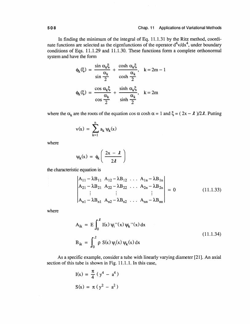
As a specific example, consider a tube with linearly varying diameter [21]. An axial section of this tube is shown in Fig. 11.1.1. In this case,

I(x) = ~ ( y4 - a4 )

S(x)=x(y2 -a2 )


where

R-r ( 1) y=R- l x=R- ~+2 (R-r)

The coefficients Aik and Bik of Eq. 11.1.34 are thus

Aik = ~ { [ ..!.. ( R + r f - a4 J ~~) - .!. ( R + r )( R - r ) ~~ 4..t3 16 2

+; (R + rf(R- rfi~r- 2(R + r)(R- rfi~r

+ (R - r f I~f}

{ [ ( R + r f 2 ] -(o) Bik = xpl -~4--- a Iik

1 2 2 -(1) ~ -(2) } - S ( R - r ) Iik + ( R - r J Iik

where ~~~) and if~ are the integrals

Jl/2 If~>= ~n<l\"(~)fl>k"(~)d~, n=0,1,2,3,4

-1/2

- Jl/2 ~~ = ~n <1\(~) <Pic(~) d~, -1/2

n = 0, 1, 2

-t

- --- 2r

+

Figure 11.1.1 Tapered Beam

For numerical calculations, the following dimensions are adopted for the tube: l = 4000 mm, R = 400 mm, r = 200 mm, a= 100 mm.


Putting n = 1, 2, and 3 in

and evaluating terms in Eq. 11.1.33, detailed calculations [21] yield the following equations for A.:

(1) 0.8526-0.1917 X 109 A ~ = 0

(2) 0.8526-0.1917 X 109 A~ - 1.5341 + 0.0632 X 109 A~ = 0

- 1.5341 + 0.0632 X 109 A~ 39.4262 + 0.3526 X 109 A~

(3) 0.8526-0.1917 x109 A.f -1.5341 +0.0632 x109 A.f 1.1077 +0.0037 x109 A.f -1.5341-0.0632xl09 A.f 39.4262+0.3526xl09 A.f -26.614+0.0865xl09 A.f =0

1.1077-0.0037 x109 A.f -26.614 +0.0865 x109 A.f 156.59 +0.3168 x109 A.f

the smallest roots of which are

A.~l) = o.4446 x 10-8 E p

A.~2> = o.4226 x 10-8 E p

A.~3> = 0.4171 x 10-8 ~ p

Note that the successive values of A.1 converge rapidly. The relative error in passing from A.1 (l) to A.1 <3> is about 5% and in passing from A.1 (Z) to A.1 <3>, it is about 1.3%. For the second eigenvalues, the approximate values are

A.~2> = 11.628 x 10-8 ~ p

A.~> = 11.074 x 10-8 E p

and the relative error in passing from "-2(2) to "-2(3) is approximately 5%.

Sec. 11.2 Second Order Partial Differential Equations 511

11.2 SECOND ORDER PARTIAL DIFFERENTIAL EQUATIONS

Boundary Value Problems for Poisson and Laplace Equations

Consider the Poisson equation

(11.2.1)

where x is a point in a bounded m-dimensional region n, m = 2 or 3. Consider first the Dirichlet probl~m; i.e., find the solution of Eq. 11.2.1 that is continuous in the closed physical domain n = n + r and satisfies the boundary condition

(11.2.2)

As the domain of the Laplace operator Au = - V2u, take the linear space of functions D A that satisfy the following conditions:

(1) They are continuous, together with their first and second derivatives in the closed domain n = n + r.

(2) They vanish on r.

For the linear space DA, it was shown in Section 9.2 that the operator- V2 is positive definite.

It follows that the Dirichlet problem of Eqs. 11.2.1 and 11.2.2 is equivalent to the problem of minimizing the functional

F(u) = ( - V2u, u ) - 2 ( u, f)

Integrating by parts and using the boundary condition of Eq. 11.2.2, this is

F(u) = JD { (Vu f- 2uf} dO (11.2.3)

As shown in Section 6.3, the problem of the deflection of a membrane that is fixed at its edge, under the influence of a normal load, reduces to Eqs. 11.2.1 and 11.2.2, where f(x) is proportional to the loading. The functional of Eq. 11.2.3 is proportional to the potential energy of the deformed membrane. Thus, the Minimum Functional Theorem is just the principle ef minimum total potential energy.

A similar result is obtained if, in place of Eq. 11.2.2, the boundary condition for the mixed problem,

(11.2.4)

is applied, where a(x) is a non-negative continuous function that is not identically zero. For this problem, the domain of the Laplace operator is denoted as the linear space Ma of


functions that satisfy the boundary equation of Eq. 11.2.4 and the same conditions of continuity and differentiability as functions in the linear space DA. To show that, with domain Mo. the operator - V2u is also positive definite, note that

(- V2u, u) = - Ir u ~ dS + Ia (Vu r dQ

= Ir <ru2 dS + Io ( Vu r dO ~ 0

If ( - V2u, u ) = 0, then it is necessary that

From the second equation, it follows that u = c, a constant. Substituting this in the first equation,

Since the function a(x) is continuous, non-negative, and not identically zero, it follows

that J r adS > 0, so c = 0. Thus, u(x) = 0, for all X in n, so the operator Au = - V2u

with domain Mo is positive defmite.

The problem of integrating the Poisson equation of Eq. 11.2.1, subject to the boundary condition of Eq. 11.2.4, can now be replaced by the problem of minimizing the functional

F(u) = (- V2u, u ) - 2 ( u, f)

= J 0 { ( Vu f - 2uf } dQ + J r <ru2 dS (11.2.5)

over the linear space Ma· Actually, the boundary condition of Eq. 11.2.4 is natural, so it can be ignored in minimization of the functional ofEq. 11.2.5.

Finally, a solution of the Neumann_ problem for Eq. 11.2.1 is sought that is continuous and continuously differentiable in 0 and that satisfies the free edge boundary condition

~I = o dn r (11.2.6)

Define a linear space Mo that consists of functions that satisfy Eq. 11.2.6 and the same conditions of continuity and differentiability as the functions of the linear space D A· How-


ever, the operator- V2u will not be positive definite on this linear space. In fact,

(11.2.7)

From the equality ( - V2u, u ) = 0, it does not follow that u = 0. Indeed the function u = 1 clearly belongs to the linear space M0 and ( - V2u, u ) = 0.

To resolve this problem with positive definiteness of the Laplace operator on Mo. the Theorem of the Alternative [18, 22] is used (see discussion in Section 3.1 for matrices and discussion following Theorem 10.6.2). The Laplace operator on Mo is symmetric, so it is required that

for all solutions u of

Note that

- V2u = 0, inn

au - 0 on r on - ,

u(x) = c "* 0

(11.2.8)

is a solution of this problem. Substituting this result into Eq. 11.2.8, it follows that

(11.2.9)

That is, the Neumann problem of Eqs. 11.2.1 and 11.2.6 is solvable only if the applied force f satisfies Eq. 11.2.9. Further, if this problem is solvable, it has an infinite number of solutions, all differing from one another by a constant. To obtain a unique solution u(x), it is required that

In u(x) dQ = 0 (11.2.10)

Considering the Neumann problem for Eq. 11.2.1, the domain of the Laplace opera-tor is defined as the linear space ~ of functions that

(1) are continuous, together with their first and second derivatives inn. (2) satisfy Eq. 11.2.6. (3) satisfy Eq. 11.2.10.


It will next be proved that the operator- V2u is positive definite for all functions in the linear space~· For any u in~. Eq. 11.2.7 holds. If (- V2u, u) = 0, then from Eq. 11.2.7, u =c. But Eq. 11.2.10 implies c = u = 0. Thus, the operatoris positive definite.

This Neumann problem can thus be replaced by the variational problem of finding the function in ~ that minimizes

F(u) = ( - V2u, u ) - 2 ( u, f)

or, by virtue of the boundary condition of Eq. 11.2.6,

F(u) = In { ( Vu 'f - 2fu} dQ (11.2.11)

The boundary condition of Eq. 11.2.6 is natural, so the functional of Eq. 11.2.11 can be minimized without regard for boundary conditions.

It is often required to solve the Laplace equation with non-homogeneous boundary conditions. It was shown in Section 10.5 that integration of the Lapiace equation in the domain Q, under the boundary condition of the Dirichlet problem

u I r = g(x) (11.2.12)

reduces to finding the minimum of the functional

(11.2.13)

over the set of functions that satisfy Eq. 11.2.12. If the boundary condition has the form of the Neumann problem

dU I an r = h(x) (11.2.14)

then the problem reduces to finding the minimum of the functional

In (Vufdn- 2 IruhdS (11.2.15)

without regard to boundary conditions. Note that in the case of boundary conditions of the mixed problem; i.e.,

[ ~~ + o(x)u Jr = h1(x) (11.2.16)

the energy functional has the form

F(u) = J ( Vu )2 dQ + J ( ou2 - 2uh1 ) dS n r

(11.2.17)


The positive definite character of the operator - V2u has been established here for each of the domains D A• Mo. Mo. and ~. However, in order to be able to use the Ritz method with full confidence, it is important to establish that the operators are positive bounded below. It was shown in Section 9.2 that the Laplace operator is positive bounded below over the set D A· It is shown in Ref. 21 that the Laplace operator is also positive bounded below over the domains Mo and Mo.

Torsion of a Rod of Rectangular Cross Section

The problem of torsion of a rectangular rod is considered in some detail, because a relatively simple exact solution is known [26], to which approximations can be compared. This problem reduces [23, 26] to integration of the Poisson equation

in the rectangle -a ~ x 1 ~ a, - b ~ x2 ~ b, under the boundary conditions

u(±a, xz) = u(x1, ±b) = 0

(11.2.18)

(11.2.19)

From symmetry, it is clear that the function u is even in both x1 and x2. A sequence of polynomials that possess this property and vanish on the edges of the rectangle; i.e., on the straight lines x 1 = ±a, x2 = ± b, has the form

(11.2.20)

Restricting attention to three terms, the approximate solution will be of the form

Performing the necessary calculations [21], the Ritz equations for the unknowns a1,

~.and a3 are

128 5 3 [ a2 b2 ] 128 5 5 [ 11 2 1 2 J 45 a b 7 + T a1 + 45 x 7 a b T b + 3 a az


128 3 3 [ a2 b2 J 128 5 5 ( 2 2 ) 45 a b 5 + T a1 + 45 x 35 a b a + b a2

128 [ 11 2 1 2 J 16a3b5

+ 45 x 7 5 a + 3 b a3 = 45

The solution of these equations is

35 ( 9a4 + 130a2b2 + 9b4 )

al = -----------------------------16 ( 45a6 + 509a4b2 + 509a2b4 + 45b6 )

105 ( 9a2 + b2 ) a2 = ------------------

16 ( 45a6 + 509a4b2 + 509a2b4 + 45b6 ) (11.2.21)

105 ( a2 + 9b2 ) a3 = ----------------

16 ( 45a6 + 509a4b2 + 509a2b4 + 45b6 )

If only one coefficient a1 were used; i.e., if

then

A similar calculation can be performed to obtain a two term approximation. A second sequence of coordinate functions that are even and satisfy the boundary

conditions is

where i and j are odd integers. These functions are energy orthogonal, since

- f_bb J:a 4Pmn V2<1\:s dxt dx2

(11.2.22)

= ~2 [ ~ + ~ ] [ r, COS m;:l COS ~I dx1 ]

x [ J ~ cos n;:2 cos •;:2 dx2 ]

= 0, if rn '#. r or n '#. s


Since the coordinate functions are orthogonal, the Ritz equations are decoupled and easily solved. Direct calculation [21] yields the following one, three, and six term approximations:

64a2lf [ 1 1tX l 1tX2 u3(x1, x2) = -;.r- a2 + b2 cos 2a cos 2b

1 1tX l 31tXz 1 31tX 1 1tX2 ] + cos-cos-+ cos-cos-

3 ( 9a2 + b2 ) 2a 2b 3 ( a2 + 9b2 ) 2a 2b

1 n:x l 3n:x2 1 3n:x 1 1tX2 + 2 2 cos -2a cos -2b + 2 2 cos -2a. cos -2b

3 ( 9a + b ) 3 ( a + 9b )

1 5xx 1 n:x2 ] + .. cos-cos-

5 ( a2 + 25b2 ) 2a 2b (11.2.23)

With the aid of these approximate solutions, two mechanical characteristics of the torsional problem can be calculated, namely the torque and the maximum tangential stress, as functions of a. These values for the approximate solutions can be obtained and compared with known exact solutions. From Ref. 26, the torque required to create a twist of o: rad. per unit length of the rod is

T = 4GaJb fa udx1 dx2 -b -a

which can be represented in the form

(11.2.24)

(11.2.25)

where y = b/a and k1 (y) is a nondimensional factor. Forb > a, the maximum tangential stress in the rectangular section occurs half-way along the side [26]. The greatest tangential stress 1: is [26]

5 1 8 Chap. 11 Applications of Variational Methods

du t = - 2Ga ail = 2Gaa k(y) (11.2.26)

where k(y) is a nondimensional factor. For numerical comparison with known solutions, denote the nondimensional ap

proximations obtained above with the polynomial and Fourier coordinate functions as (~ (i), k1 (i)) and (kt>, k1r(i)), respectively. For the Fourier approximation, numerical evaluaticin of the integral in Eq. 11.2.24, using the notation of Eq. 11.2.25, yields the approximations

kl (3)(y) = 256y2 [ 1 + 1 + 1 ] f 1t6 1 + 'Y2 9 ( 9 + 'Y2 ) 9 ( 1 + gy2 )

256y2 [ 1 + __ 1 __ + ___ 1 __

1t6 1 + y2 9 ( 9 + y2 ) 9 ( 1 + 9y2 )

+ 1 + 1 ] 25 (25 + y2 ) 25 (1 + 25y2 )

Likewise, presuming b;;::: a, the maximum shear stress occurs at (a, 0). Evaluating Eq. 11.2.26 at this point, where a;an = a;axh yields the approximations

kj6>(y) = 32y2 [ 1 - 1 + __ 1_

1t3 1 + 12 3 c r + 9 > 1 + 912

+ _5_(_-y2_1_+_2_5_) + 1 + 12Yy2 ]


Tables 11.2.1 and 11.2.2 provide a comparison of the exact values [26] of the quantities k1 and k with their approximate values.

Table 11.2.1 Fourier Approximate Values of k1

kl k (1) lr

k (3) lr

k (6) lr

1 0.1406 0.133 0.139 0.1401 2 0.229 0.213 0.225 0.228 3 0.263 0.240 0.258 0.261 4 0.281 0.251 0.273 0.278 5 0.291 0.256 0.281 0.287 00 0.333 0.266 0.299 0.311

Table 11.2.2 Fourier Approximate Values of k

y k kP) kP) kr(6)

0.675 0.516 0.585 0.613 2 0.930 0.826 0.831 0.870 3 0.985 0.929 0.870 0.931 4 0.997 0.971 0.865 0.954 5 0.999 0.992 0.854 0.961 00 1.000 1.032 0.803 1.012

Tables 11.2.1 and 11.2.2 show that the approximate solutions give fairly good values of the torque, but poorer values for the maximum tangential stress. This applies particularly to u3(x1, x2). This is caused by the fact that the precision of the evaluation of the torque k1 depends on the rapidity of convergence of the series in the mean, whereas the precision of the evaluation of k depends on the rapidity of uniform convergence of the series of derivatives. It is seen that the series converges in the mean fairly rapidly, but that the convergence of derivatives of this series is slow.

For comparison, values of k1 (l)(y), k1 (3)(y), ~ (l)(y), and kP <3)(y), evaluated from the polynomial approximations, ke given in Tables 11.2.3 and 11.2.4.


Table 11.2.3 Table 11.2.4 Polynomial Approximate Polynomial Approximate

Values of k1 Values of k

'Y k1 k (1)

1p k (3)

1p 'Y k kp (1) kp (3)

1 0.1406 0.139 0.1404 1 0.675 0.625 0.703 2 0.229 0.222 0.228 2 0.930 1.000 0.951 3 0.263 0.250 0.263 3 0.985 1.125 0.982 4 0.281 0.261 0.279 4 0.997 1.176 0.969 5 0.291 0.267 0.290 5 0.999 1.202 0.951 00 0.333 0.278 0.311 00 1.000 1.250 0.875

Comparison of Tables 11.2.1 - 11.2.4 shows that, for this application, an approximation of the same order with polynomials gives better results than with trigonometric functions for torque, and worse approximations for the maximum tangential stress. However, this circumstance may not be valid for approximations with greater numbers of terms.

11 .3 HIGHER ORDER EQUATIONS AND SYSTEMS OF PARTIAL DIFFERENTIAL EQUATIONS

The power of variational methods becomes even more clear for problems that are described by higher order partial differential equations and systems of second order partial differential equations. The basic operator properties of equations that govern such systems are the same as for tiae simpler ordinary and second order partial differential operator equations studied in the preceding sections. More important, the Ritz method offers a practical method of solving such problems, with the aid of the modern high speed digital computer. The examples presented in this section are intended to illustrate the power and generality of the Ritz method.

Bending of Thin Plates

The equation for bending of a thin elastic plate may be written as [24]

(11.3.1)

or in more detailed form,

Sec. 11 .3 Higher Order Equations and Systems of Partial Differential Equations 52 1

Here, u(x1, x2) is the lateral deflection of the plate, f(x1, x2) is the intensity of the normal load on the plate, and

Eh3

D= -----12 (1 - cJl)

where E and o < 1 are Young's modulus and Poisson's ratio for the material from which the plate is made and his its thickness. The region covered by the plate in the (x1, x2)

plane is denoted by 0, with boundary r. Depending on the manner of support of the plate edge, the following boundary conditions are most frequently encountered [24]:

(a) The edge of the plate is clamped;

ulr = 0

au I = 0 an r

(b) The edge of the plate is simply supported;

ulr = 0

a2u (a2u 1 au) an2 + (J a-r + p an r = 0

(11.3.2)

(11.3.3)

fu Eqs. 11.3.2 and 11.3.3, n and t are the exterior normal and tangent to r, respectively, and pis the radius of cutvature of the boundary r. Different parts of the edger may be fixed differently. Accordingly, r can be split into several parts, on each of which either Eq. 11.3.2 or Eq. 11.3.3 holds.

If at least one ofEqs. 11.3.2 or 11.3.3 holds on each part of the boundary r, the energy functional is

F(u) = (Au, u ) - 2 ( u, ~ )

(11.3.4)


If the entire boundary of the plate is clamped~ the functional of Eq. 11.3.4 can be represented in either of the following simpler forms:

F(u) = ( Au, u ) - 2 ( u, ~ )

= J J 0 [ ( V2u f - ~ u J ciD

= Jt[(~:~r + 2(d!~J2 + (~ir- ~+a (11.3.5)

Clearly, for the case of a clamped boundary, (Au, u) :=:: 0. If (Au, u) = 0, all the second derivatives of u are zero in 0. In particular,- V2u = 0. Since u = 0 on r, this implies u = 0 in 0. Thus, the bihannonic operator with clamped boundary conditions is positive definite. While not shown for other boundary conditions, the same result holds. In fact, the operator is positive bounded below [18].

The foregoing results show that the problem of bending of a plate is equivalent to minimizing the energy functional over the set of functions in the class HA that satisfy Eqs. 11.3 .2 on the clamped part of the boundary and the condition u lr = 0 on the simply supported part of the boundary. The remaining boundary condition is natural and need not be satisfied by coordinate functions.

If the plate has variable thickness h(x), then Eq. 11.3.1 is replaced by

+ iP ( h3 a2u ) + 2 < 1 _ 0 ) a2 ( h3 f12u ) = _!_ axi axi dx1 dx2 dx1 dx2 D'

(11.3.6)

where

E D' = -----

12 ( 1 - cJl)

The boundary conditions on the clamped or simply supported segments of the boundary have the same form as for a plate of constant thickness. If the thickness h of the plate is nonzero, the operator of Eq. 11.3.6 is positive definite on the set of functions that satisfy Eqs. 11.3.2 and 11.3.3 on the clamped and simply supported parts of the boundary, respectively. The corresponding variational problem consists of minimizing the integral

Sec. 11.3 Higher Order Equations and Systems of Partial Differential Equations 52 3

(11.3.7)

subject to the conditions of Eqs. 11.3.2 on the clamped part of the boundary and the condition u lr = 0 on the simply supported part of the boundary.

If the thickness of the plate is constant the frequency of vibration of a thin elastic plate is proportional to the eigenvalues of the biharmonic operator; i.e.,

V4u = a4u + 2 a4u + a4u = A.hu

axt axr ax~ ax~

subject to the boundary conditions of Eqs. 11.3.2 or 11.3.3. For the general case, the boundary of the plate is split into segments r 1 and r 2, on which Eqs. 11.3.2 and 11.3.3, respectively, are satisfied.

The smallest eigenvalue of the bihannonic operator is the minimum value of the functional

the minimum taken over the set of functions that satisfy

( Bu, u ) = J J 0 hu2 dO = 1

and the boundary conditions

~, = 0 dn r

1

(11.3.9)

(11.3.10)

If the entire boundary of the plate is clamped, the smallest eigenvalue of the biharmonic operator is equal to the minimum of the functional


where the function u(x) satisfies Eq. 11.3.9 and the boundary conditions u lr = 0 and ( du/dn ) lr = 0.

The nth eigenvalue "-n of the biharmonic operator is related to the nth natural frequency Oln of the plate by the expression [24]

y~ "-a= n

where y is the density of the plate and D is the resistance of the plate to bending. If the thickness h of the plate varies, the equation for natural vibration of the plate

takes the fonn

(11.3.11)

where the parameter A. is related to the natural frequency ro by the expression [24]

A. = 12 (1 - ci ) y of E

The smallest eigenvalue A.1 is the minimum of the functional

subject to the conditions of Eqs. 11.3.9 and 11.3.10.

Bending of a Clamped Rectangular Plate

Lateral displacement u of a plate satisfies the biharmonic equation

4 f Vu=-=p

D (11.3.13)


where f is the load intensity and D is the rigidity of the plate, subject to the boundary conditions

ulr = 0

au I = o an r

(11.3.14)

The lengths of the sides of the plate are 2a and 2b, where the coordinate axes are parallel to the sides of the plate and the origin of coordinates is at the center of the plate.

As was shown in Eq. 11.3.5, this problem reduces to finding the minimum of the functional

(11.3.15)

over the space of functions that satisfy Eqs. 11.3.14. This problem can be solved by the Ritz method. In order to simplify calculations, suppose that the load is distributed uniformly; i.e., p =constant.

As coordinate functions, consider polynomials of the form

(11.3.16)

Odd powers of x1 and x2 are omitted, because the solution u(x1, x2) must be symmetric about the coordinate axes.

Restricting attention to three terms in Eq. 11.3.16,

the three term Ritz approximation is

The Ritz equations in this case have the form

3

I. ( V2~, V2<i>m) ak = p ( 1, <l\n ), m = 1, 2, 3 (11.3.17) k=l

Performing the necessary calculations, Eq s. 11.3.17 are [21]


( 2 1 4) ( 1 1 ) 2 ( 1 y 4 ) 2 y + y2 + 7 al + 7 + 11 y4 b az + 7 + 1T a a3

7

( y2 1 ) ( 3 4 4 ) 2 1 4 2 T + 11 r al + 7 + 143f + 77r b a2 + 77 c 1 + y ) a a3

1

where y = b/a. If the plate is square, then y = 1 and these equations assume the simpler form

18 18 2 18 2 7 T al + 77 a az + 77 a a3 = 128a4 p

18 502 2 2 2 1 77 al + 1001 a a2 + 77 a a3 = 128a4 p

18 2 2 502 2 1 77 al + 77 a a2 + 1001 a a3 = 128a4 p

Solving this system,

( x21 + xz2 J P(2 2)2(2 2-.2 u ::::: u3 = a4 x1 - a x2 - a J 0.02067 + 0.0038 a2

The approximate deflection at the center of the plate is thus

u3 1 = 0.02067pa4 x1=0,x2=0

If the approximation for u were restricted to one term; i.e.,

then the Ritz equations reduce to the single equation


( 2 1 4) 7 'Y + 2 + 7 a1 = 2 2 P

'Y 128a b

so

49

which gives the value

=

for the deflection at the center of the plate. In the case of a square plate (a= b),

u1 I = 0.02127pa4 xl":O,x2=0

Note that u1 and u3 give similar values at the center of the plate, suggesting that u3 is a good approximation of the solution.

Computer Solution of a Clamped Plate Problem

To illustrate the effect of the number of coordinate functions used in solving problems with the Ritz technique, the clamped plate with both constant thickness and variable thickness is solved for displacement due to a uniformly distributed lateral load f and for the fundamental natural frequency and the associated eigenfunction. In these problems, static deflection is governed by the differential equation of Eq. 11.3.6 and the boundary conditions of Eqs. 11.3.10. For vibration, the deflection satisfies Eq. 11.3.11 and the same boundary conditions. Since all boundary conditions in Eqs. 11.3.10 are principal, the coordinate functions must satisfy them.

Since the problem is symmetric, the following even trigonometric coordinate functions are selected:

M M _ ~ ~ ' ( 2m - 1 ) 1tX l 1tX l ( 2n - 1 ) 1tX2 1tX2

UM - ..t.J ..t.J amn COS a COS a COS b COS b m=l n=l

M M 1 ""' ~ ( 2mxx1 = 4 L..J £...J 8mn cos a

m=l n=l

( 2m - 2 ) 1tx 1 ) +cos-----

a

( 2nxx2 ( 2n - 2 ) xx2 ) X COS b + COS b

(11.3.18)


The Ritz equations for this fonnulation are

l tf 8mn lb Ja o{ [ { ( ~ )2 cos 2mxxl 2 m=l n=l -b -a a a

( (2m - 2) 1t )2 (2m-2) 1tXt } + cos-----

a a

{ 2nn2 ( 2n- 2) xx2 } { 2mn1 (2m - 2) xx1 } x cos-+ cos + v cos-+ cos-----

b b a a

x { (~)2 2m1tx2 ( (2m_ 2) x)2 (2m-2) xx2 } b cos b + b cos b

{ ( 2k1t ) 2 2k1tXt ( ( 2k- 2) 1t ) 2 ( 2k- 2) 1tXt } + - cos- + cos-----

a a a a

{ Un2 ( 2.t - 2) xx2 } ] [ ( 2m1tx1 ( 2m - 2) n 1 ) X COS - + COS + COS - + COS -----

b b a a

{ ( 2m7t)2 2m1tx2 ( (2m-2) 1t)2 (2m-2) 1tx2} X b COS---.;-- + b COS --~b--

{ ( 2m1t )2 2mnt ( (2m - 2) 1t )2 (2m - 2) 1tXt } + v ....._ cos- + cos-----

a a a a

( 2mn2 ( 2m - 2 ) xx2 ) ( 2kn1 ( 2k- 2 ) 1tX1 ) x cos -.;-- + cos b cos --;- + cos a

2

{ ( ~)2 2.tn2 + ( ( 2.t - 2 ) 1t) ( 2.t - 2 ) 1tx2 } x b cosb b cos b

( 2m1t . 2m1txt ( 2m - 2 ) 1t . ( 2m - 2 ) 1tXt ) + 2(1-v) -sm- + sm-----

a a a a

( 2m1t . 2m1tx2 ( 2m _ 2 ) 1t . ( 2m - 2 ) xx2 ) x bsm-.;- + b sm b

( 2k1t . 2k1tXl ( 2k _ 2 ) 1t . ( 2k - 2) 1tXt ) x -sm- + sm-----

a a a a

( 2.t1t . 2.t1tX2 ( 2.t - 2) 1t . ( 2.t - 2 ) 1tX2 ) ] } x b sm --.;- + b sm b dx1 dx2

1 Jb 1a ( 2k1txl ( 2k- 2) 1tX2 ) ( 2.t1t. x2 ( 2.t - 2) n 2 ) = -2 f cos - + cos cos - + cos b dxl dx2, -b-a a a b

k = 1, 2, ... , M, 1 = 1, 2, ... , M (11.3.19)

These equations were programmed and solved for a square plate (b ::::: a), with 9 and 16 coordinate functions; i.e., M = 3 and M = 4, respectively. Results for deflection and bending moment Mx1 at the points of interest shown in Fig. 11.3.1 and for the smallest eigenvalue for a square plate of constant thickness are given in Table 11.3.1. The Ritz eigenvalue equations were also solved for the eigenvalue C = pco2, where pis the mass


density of material and ro is the natural frequency, in rad/sec. Results are presented in Table 11.3.1. Note that the polynomial three term approximation for deflection was 0.0206 ( fa4/D ), whereas the 16 term approximation here gives 0.0201 ( fa4/D ). Note also that while accurate displacement and eigenvalues are obtained, since bending moment involves two derivatives of displacement [26] (see also Eq. 11.4.11), it is less accurate.

Table 11.3.1 Results for Clamped Plate (Constant Thickness)

Mxt@A Mxt®B u@A ~ = pro2

x4fa2 x4fa2 16fa4 1J£ x- x 4a2 ph D

M=3 0.025092 -0.038922 0.0012626 36.106

M=4 0.021518 -0.041473 0.0012586 36.044

Solution [26] 0.0231 -0.0513 0.00126 35.98

T a

_t_ A..._ ___ B-1-- Xt

Figure 11.3.1 Points of Interest on Plate

The same problem was solved for a clamped plate of variable thickness, with

h(x) = 2 ( 1 - I :tl ) ( 1 - I :2 I ) ho

The same coordinate functions, with 4, 9, and 16 terms (corresponding toM= 2, 3, and 4, respectively) were used to solve this problem. Numerical results are given in Table 11.3.2.


Table 11.3.2 Results for Clamped Plate (Varying Thickness)

MXt@A MXt@B u@A ~ = pm2

x4fa2 x4fa2 16fa4 1~ XJ5* X~ Pho

M=2 0.029754 -0.0062549 0.00060060 40.706

M=3 0.063371 -0.0085592 0.00065468 39.376

M=4 0.040864 -0.010112 0.00067205 38.774

Eil6 *D=----

12 ( 1 - v)

11.4 SOLUTION OF BEAM AND PLATE PROBLEMS BY THE GALERKIN METHOD

To illustrate use of the Galerkin method, problems of the type treated in Section 11.3 for beams and plates are solved numerically using the Galerkin method.

Static. Analysis of Beams

The governing equations of a beam may be written in the second order form

dx2

d2u M (11.4.1)

- dx2 - EI

or in the more usual fourth order form

(11.4.2)

where u is deflection, M is moment, E is Young's modulus, I is moment of inertia of the beam cross section, and f(x) is distributed load, taken as constant in the examples treated here.

Sec. 11.4 Solution of Beam and Plate Probtems by the Galerkin Method 531

The second order form of Eq. 11.4.1 has the advantage that both displacement u and moment M are determined with comparable accuracy. This feature allows direct computation of bending stress in the beam, without having to compute derivatives of an approximate numerical solution u(x), as was done in the case of plates in Tables 11.3.1 and 11.3.2.

As has been shown, under the usual boundary conditions, the fourth order operator of Eq. 11.4.2 is symmetric and positive definite. For the second order operator of Eq. 11.4.1, under the usual boundary conditions,

c:r~r A[~] dx = t:: (-OM' - Mu" - ~ )dx

= f_:: ( -uM"- Mu" - ~ )dx

so the operator A is symmetric. However,

f 112 [ u]T A[ u] dx = JJ./2 [ 2u'M' - M._EI2 ] dx -J./2 M M -J./2

may be made negative by choosing admissible u' and M' that are orthogonal, so the frrst term vanishes and a negative integral results. Thus, the second order operator A is not positive definite and the Ritz method cannot be used directly for this formulation.

Simply Supported Beam

Two simply supported beam problems are solved using the Galerkin method. One has a uniform cross section and the other has a varying cross section, with area

( lxl) .l .l a(x) = 2an 1 - - - - < X< --v .l ' 2 2

and moment of inertia I(x) = a [ a(x) ]2, which is symmetric with respect to the center of the span. The boundary conditions are

(11.4.3)

Under symmetric loading, the solution will be symmetric, so cosine functions are


selected as coordinate functions. This leads to the approximate solutions

f ( 2n- 1) n;x u = L...t lin cos

n=l l

f (2m -1 )n;x M = L...tbmcos---------

m=l l

(11.4.4)

Substituting these sums into the Galerkin equations of Eq. 10.10.13 and performing the necessary calculations,

f J./2 [ ii ]T [ u J -1/2 M A M dx

= ~>m ( ( 2m - 1 ) 1t )'

m=l l

f J./2 [ (2m- 1) n;x ( 2n- 1 ) n;x ] x cos cos · dx ~n J ..t

J J./2 lr ( 2n- 1 ) 1tX ] = f cos dx = 0, n = 1, 2, ... , N (11.4.5)

-1n ..t

_ - T [ ( 2n - 1 ) n:x ]T where [ u, M ] = . cos J , 0 , and

f1/2[ij]T [UJ -112 M A M dx

= i: a,. ( ( 2n - 1 ) 1t )'

n=l J

J 112 ( 2n - 1 ) n;x ( 2m - 1 ) 1tx X COO COO ~

-J./2 J J

_ ~ f 112 [ _!.._ ( 2j- 1 ) 1tX (2m -1) 1tX ] _ L...t bj EI cos cos dx- 0, j=l -J./2 ..t ..t

m = 1, 2, ... , M (11.4.6)

Sec. 11.4 Solution of Beam and Plate Problems by the Galerkin Method 533

_ - T [ ( 2m - 1 ) 1tX ]T where [ u, M ] = 0, cos .l .

Numerical results for the uniform beam are presented in the first two columns of Table 11.4.1, for six and ten coordinate functions. Similar results for a beam with variable cross section are given in Table 11.4.2. As expected, results for deflections are very accurate. While there is some error in the calculation of bending moment, it is much smaller than would be experienced if numerically determined displacements were differentiated twice.

Table 11.4.1 Results for Simply Supported Beam

(Uniform Cross Section, Second Order Method)

E~ =bending rigidity of beam -.l/2

~. ao = cross sectional area of beam 0&;~ p = mass density per unit volume

Moment@ A u@A ~ = pro2

xU2 f.t4 I~ X E~ X? pa;

N=3 0.12526 0.013021 9.86960

M=3

N=5 0.12506 0.013021 9.86960

M=5

EXACT 0.12500 0.013021 9.86960

.l/2

~/

534 Chap. 11 AppUcations of Variational Methods

Table 11.4.2 Results for Simply Supported Beam

(Varying Cross Section, Second Order Method)

A

a(x) = 2ao ( I - I ~ I )

X ),f2 10 = aa5

-.l,/2

Moment@ A u@A ~ = pro2

X f),2 f),4 xl..~ X EJo .1,2 Pao

N=3 0.12526 0.0046279 12.598

M=3

N=5 0.12506 0.0046247 12.599

M=5

Clamped Beam

Clamped beam problems are now solved, using both the second and fourth order formulations. The boundary conditions for this case are

(11.4.7)

The following coordinate function approximation, which satisfies these principal boundary conditions, is selected:

N ~ ( 2n - 1 ) 1tX 1tX

u = £...i~ cos cos-n=l ), ),

~ [ 2nxx ( 2n - 2 ) xx ] = £...i ~ cos- + cos----~1 ), ),

(11.4.8)

~ (m-1 )xx M = £...J bm COS----

m=l ),


where u and M are represented in symmetric form. Substituting the above into the Oalerkin equations of Eq. 10.10.13 and carrying out

the necessary computation yields

J 1/2 [ u]T [ u] -112 M A M dx

= t. bm J J!./2 [ ( ( m - 1 ) re J2 cos 2nrex m=O -J./2 ,t ,t

2

( ( m - 1 ) re J ( 2n - 2 ) rex ] ( m - 1 ) rex + ~ ~ ~

,t ,t 1

f112 [ 2nrex ( 2n- 2) rex J = f cos - + cos dx,

~n J J n = 1, ... , N

(11.4.9)

- T T where [ u, M ] = [cos 2nrex/ .t + cos { ( 2n - 2 ) rex/ 1 } , 0 ] , and

J J./2 [ u ]T [ u J _112 M A M dx

LN J J!./2 r ( 2nre \2 2nrex = ~ -'cos-

n=l -,t/2 L ~ J ) 1

( ( 2n - 2 ) re J2 ( 2n - 2 ) rex ] ( m - 1 ) rex + cos cos dx

J 1 1

_ ~ . J J./2 2. . ( j - 1 ) rex ( m - 1 ) rex _ L..J bJ EI cos cos dx- 0, j=l -J./2 1 ,t

m = 1, ... , M (11.4.10)

- T T where [ ii, M ] = [ 0, cos { ( m- 1 ) rex/ J } ] .

Inserting the first of Eqs. 11.4.8 into the Oalerkin equations of Eq. 10.10.13 for the fourth order operator and performing the necessary calculations yields

f J.t/2 1 EI{ (2nre)2 2mtx ( (2n-2)n: )2 (2n-2)rex} L..i a - - cos--+ cos----n=O n -J./2 2 1 1 J 1

{ ( 2kre )2 2krex ( ( 2k - 2 ) 1t J2 ( 2k - 2 ) rex } x - cos- cos dx J ,t 1 1

f 1.!2 [ 2krex = f cos--

-J./2 . l

( 2k- 2) rex ] + cos dx,

l

k = 1, ... , N (11.4.11)


The second order approximate solution of Eqs. 11.4.9 and 11.4.10 and the fourth order approximate solution of Eqs. 11.4.11 were solved numerically for uniform and tapered clamped beams. Results for varying numbers of coordinate functions are given in Tables 11.4.3 and 11.4.4. Note that displacement results are accurate with both second and fourth order formulations, slightly more accurate with the fourth order formulation. Bending moments, in contrast, are much more accurate with the second order formulation. This is due partly to error induced in differentiating numerically computed displacements to obtain bending moments in the fourth order formulation.

Table 11.4.3 Results for Clamped Beam (Uniform Cross Section)

A

-.I. /2 X .1,(2

Moment@ A Moment@B u@A '= pro2

xU2 xU 2 f.l.4 I~ x Elo x .1.2 Pao

N=3 0.041676 -0.083179 0.0026213 22.374

M=4 2nd Order

N=5 0.041668 -0.083404 0.0026131 22.373

M=6

N=5 0.042485 -0.074147 0.0026023 22.383 4th Order

N=lO 0.041185 -0.078765 0.0026023 22.374

Exact 0.041667 -0.083333 0.0026042 22.373


Table 11.4.4 Results for Clamped Beam (Varying Cross Section)

a(x) = 2ao ( I - ~ ) A

Io=a~ -J./2 X J./2

Moment@ A Moment@B u@A '= pm2

X f),2 X f),2 f),4 I~ X Elo x-;z Plio

N=3 0.056862 -0.067993 0.0013586 23.410

M=4 2nd Order

N=5 0.056855 -0.068216 0.0013476 23.413

M==6

4th Order N=5 0.061550 -0.053045 0.0013252 23.487

N= 10 0.056509 -0.060293 0.0013320 23.428

Static Analysis of Plates

The governing equations for bending of a plate [24] can be written in the second order form

a2u 12 12 ----M +v-M axr Eh3 XI Eh3 Xz

a2u 12 12 ----M +v-M

ax~ Eh3 Xz Eh3 XI

u

a2u 24 (1 + v) 2 - M axl dXz Eh3 xlx2

=

0 0 0

f(x 1, x2)

(11.4.12)


where Mx and M are bending moments on cross sections normal to the x1 and x2 axes, Mx1~ is a \orsion:f moment, u is deflection, his thickness of the plate, vis Poisson's ratio, E is Young's modulus, D = Eh3/[ 12 ( 1 - v) ], and f is the distributed applied load. Equations 11.4.12 apply to plates with varying thickness. The applied load f is taken as uniformly distributed in the examples treated here.

Simply Supported Plate

Simply supported plates with uniform and varying thickness are solved using the second order equations of Eqs. 11.4.12. The boundary conditions are

u(± a, x2) = u(x1, ±b) = 0 (11.4.13)

The solution is approximated by the following coordinate function expansions:

f f . ( 2m - 1 ) xx1 ( 2n - 1 ) xx2 Mx1 = ~ ~ 3.mn COS 2a COS 2b

m=l n=l

f f . ( 2m- 1 ) xx1 ( 2n - 1 ) xx2 Mx2 = ~ ~ bmn cos 2a cos 2b

m:.::l n=l

M N ~ ~ . mxx1 . nxx2

Mx1x2 = ~ ~ Cmn sm ~ sm 2b m=l n=l

M N ~ ~ . ( 2m- 1 ) xx1 ( 2n - 1 ) xx2

u =~~~cos 2a cos 2b m=l n=l

(11.4.14)

where the coordinate functions are chosen so that Mx1, Mx2, and u satisfy the principal boundary conditions. Note that since the moment Mx1x2 is antisymmetric, its coordinate functions are selected in antisymmetric form.

Substituting Eqs. 11.4.14 into the Galerkin equations of Eq. 10.10.13 and carrying out necessary computations,

1 [ Mx , ~ , ~ x , U 1 A [ Mx , ~ , ~ x , U ]T dO 0 1 2 12 1 2 12

M M 2

= In ~ ~ { ~ ( ( 2m ~ 1 ) 1t ) - ~~3 8mn + V ~~3 bmn}

( 2m - 1 ) xx1 ( 2n - 1 ) xx2 ( 2a - 1 ) xx1 ( 2P- 1 ) xx2 X COS 2a COS 2b COS 2a COS 2b dQ = 0,

a, p = 1, ... , M

- - - _ T [ ( 2a- 1 ) 1tX1 ( 2~- 1 ) 1tXz JT where [ Mx1, Mx2, Mx1 xz• u ] = cos 2a cos 2b , 0, 0, 0 ,


1 ~ ~ { ( ( 2n- 1) n; ) 2 12 12 } = n 6 f::t ~ 2b - Eh3 bmn + v Eh3 llron

( 2m - 1 ) n;x 1 ( 2n - 1 ) n;x2 ( 2a - 1 ) n;x 1 ( 2~ - 1 ) xx2 X COS 2a COS 2b COS 2a COS 2b dQ = 0,

a,~= 1, ... , M

T _ - - _ T [ ( 2a- 1 ) 7tX1 ( 2~- 1 ) 1tX2 ]

where [ Mx1, Mx2, Mx1 x2, u ] = 0, cos 2a cos 2b , 0, 0 ,

r [ Mx ' Mx • Mx X , u] A [ Mx • Mx • Mx X ' u ]T dQ Jn 1 z 1 z 1 z 1 2

M M

= 1 <L 2) <\nn (2m~ 1) 'It ( 2n ;bl) 1t

n m=l n=l l

-c 24(1+v)} mn Eh3

. mn;x1 . nn;x2 . an;x1 . ~n;x2 x sm ~ sm 2b sm ~ sm 2b dQ = 0, a,~= 1, ... , M

- - - - T [ . an;xl . ~1tX2 JT where [ Mx1, Mx2, Mx1 x2, u ] = 0, 0, sm -ra- sm -r.;-, 0 , and

M M 2 2 I L I { [ ~n ( ( 2m ~ 1 ) 7t ) + bmn ( ( 2n ;b 1 ) 1t ) J Q m=l n=l

(2m - 1 ) n;x1 ( 2n - 1 ) n;x2 ( 2a- 1 ) xx 1 ( 2B- 1 ) n;x2 X~ 2a ~ ~ ~ 2a ~ 2b

( m.n; nn; ) mn;x1 nxx2 ( 2a- 1 ) xx 1 ( 2~- 1 ) n;x2 } + 2cmn 2a Th COS ~ COS Th COS 2a COS 2b dO

1 ( 2a- 1 ) n;x 1 ( 2~- 1 ) xx2

0 f cos 2a cos 2b dO, a, ~ = 1, ... , M

(11.4.15)

where [ Mx , Mx , Mx x , u ]T == [ 0, 0, 0, cos 1 2 I 2

T ( 2a- 1 ) 1tX1 ( 2~- 1 ) 1tX2 ]

2a cos 2b ·

Numerical solutions for both uniform and variable thickness simply supported square plates are presented in Tables 11.4.5 and 11.4.6, where points of interest are defined in Fig. 11.4.1. Note that the accuracy of both displacement and bending moments is good for the uniform plate and only Mx1x2 at point C shows significant error (or slower convergence) for the variable thickness plate.

540

M=2

M=3

M=4

EXACf[26]

M=2

M=3

M=4

Chap. 11 Applications of Variational Methods

Table 11.4.5 Results for Simply Supported Plate

(Uniform Thickness, Second Order Method)

Mx1 @A Mx1x2 @ C u@A ~ = pro2

x4fa2 x4fa2 x 16fa4D 1JI x 4a2 pho

0.046895 0.033244 0.0040547

0.048235 0.032865 0.0040639

0.047709 0.032271 0.0040619

0.0479 0.0325 0.00406

Table 11.4.6 Results for Simply Supported Plate

(Varying Thickness, Second Order Method)

Mx1 @A Mx1x2 @ C u@A

19.739

19.739

19.739

19.739

~ = pro2

x 4fa2 x4fa2 X 16fa4D 1JI x 4a2 pho

0.075359 0.0054289 0.0019412 22.923

0.079413 0.0039519 0.0019674 22.942

0.080911 0.0040777 0.0019570 22.955


a -a

A B

-a

Figure 11.4.1 Points of Interest on Plate

Clamped Plate

Clamped plates with uniform and varying thickness are solved, using both the second and fornth order equations. The boundary conditions are

u(± a, x2) = u(x 1, ± b) = 0

au au ~(±a, x2) = ~(xl> ±b) = 0 ax1 ox2

(11.4.16)

The solution is approximated by coordinate functions of the form

M M

L L 2mnx 1 2nnx2 M = A cos-cos-

xi llln a b m=O n=O

M M

L L 2mnx1 2nrcx2 M = b cos-cos--

x2 mn a b m=O n=O

M M

L L . 4mrcx1 . 4nnx2 Mx x = cmn sm -- sm --

1 z a b m=l n=l

M M " " 2 ( 2m -. 1 ) nx 1 2n:x1 2 ( 2n - 1 ) nx2 2nx2

u = L..J L..J ~n cos a cos -a- cos b cos -b-m=l n=l

M M 1 ~ " [ 4mnx1 2 ( 2m - 2 ) nx 1 ] 4 £..J L..J <\nn COS - + COS ------

m=l n=l a a

[ 4nnx2 2 ( 2n - 2 ) nx2 ] X COS -b- + COS b

(11.4.17)


where u in Eqs. 11.4.17 satisfies the boundary conditions. The moments Mx1 and Mx2 are symmetric with respect to the x1 and x2 axes, so they are approximated by cosine functions. The moment Mx1x2, on the other hand, is antisymmetric and must be zero along the boundary, so its coordinate functions are selected with these properties.

Substitution of these approximations into the Galerk:in equations of Eq. 10.10.13 and performing necessary calculations yields the following equations:

M M { 4mtx2 2 ( 2n- 2) 1tx2 } 12 ~ ~ 2m1tx1 2n1tx2

X COS -b + COS b - - £...J £...J 3m COS- COS--Eh3 m=O n=O n a b

M M ) 12 2m1tx 1 2n1tx2 2a.1tx 1 2~1tx2 + V 3 L L bmn COS COS -b COS -COS -b dx1 dx2 = 0,

Eh m=O n=O a a

a..~=O,l, ... ,M (11.4.18)

- - - _ T [ 2a1tx1 2{31tx2 JT where [ Mx , Mx , Mx x , u ] = cos cos b , 0, 0, 0 ,

1 2 1 2 a

( M M [ 2 = fb Ja "" ~ (~)2 4n1t. x2 ( ( 2n _ 2) 1t) 2 ( 2n- 2) 1tx2 ] L...JL...J~n b COS b + b COS b

-b -a m=1 n=1

M M { 4m1tx1 2 (2m-2) 1tx1 } 12 L L 2m1tx1 2n1tx2

x cos-+cos -- b cos-cos-a a Eh3 mn a b m=O n=O

M M ) 12 2m1tx1 2n1tx2 2a.1tx1 2~1tx2 + v- ~""3m cos-cos- cos-cos-dx1 dx2 = 0,

Eh3 L...i £...J n a b a b m=O n=O

a.,~= 1, 2, ... , M (11.4.19)

T _ _ _ _ T [ 2a1tx1 2{31tx2 J

where [ Mx , Mx , Mx x , u ] = 0, cos cos b , 0, 0 , 1 2 1 2 a


i [ Mx , ~ , ~ x , ii] A [ ~ , M_ , ~ x , U ]T dQ n 1 2 1 2 1 --"-2 1 2

-J_:I 2 ~~ {d...[ ( 2~n) sin 4m:X' + ( (2m~ 2) • )sin 2(2m ~ 2)nx, l [ ( 2nn ) . 4nnx2 ( ( 2n _ 2 ) 1t ) . 2 ( 2n - 2 ) nx2 ]

x b sm ---r;- + b sm b

24 ( 1 + v ) . 4m1lix1 . 4nnx2 } . 4a.n:x1 . 4~nx2 - SID - sm- sm-sm- dx1 dx2 = 0,

Eh3 a b a b

a.,~= 1, 2, ... , M (11.4.20)

T _ _ _ _ T [ . 4axx1 4~1tx2 J

where [ Mx , Mx , Mx x , u ] = 0, 0, sm sin b , 0 , and 1 2 1 2 a

Jb Ja { ~ ~[ (-2mn:)2 (-2n1t)2] ~ _2nnx2 = £..J £..J 8mn + bmn b COS COS b -b -a m=O n=O a a

~ ~ ( 4mn )( 4nn) 4mnx1 4nnx2 M M } +2"-'"-'c --cos-cos-

m=l n=l mn a b a b

2 ( 2a.- 1 ) 1tXl 21tXl 2 ( 2~ - 1 ) 1tX2 21tx2 x cos a cos --;- cos b cos b dx1 dx2

Jb Ja 2 ( 2a.- 1 ) 1tx1 2nx1 2 ( 2~- 1 ) 1tX2 21tx2 = f(x 1, x2) cos cos- cos b cos -b dx1 dx2,

-b-a a a a.,~= 1, 2, ... , M (11.4.21)

where

[ 2 ( 2a- 1 ) nx1 2nx1 2 ( 2~- 1 ) nx2 2nx2 ]T

= 0, 0, 0, cos a cos -;- cos b cos b

Numerical results, obtained with both the second order and the fourth order equations for square plates, are presented in Tables 11.4.7 and 11.4.8, where points of interest are defined in Fig. 11.4.1. As in prior examples, the accuracy of displacement and bending moments is uniformly good with the second order formulation. In contrast, bending moments calculated by differentiating approximate displacements in the fourth order formulation show significant error for even the uniform thickness plate and large error for the variable thickness plate.


Table 11.4.7 Results for Clamped Plate (Uniform Thickness)

Moment@ A Moment@B u@A ~= pm2

x4fa2 x4fa2 x 16fa'TI 1-JI x 4a2 Pho

M=2 0.022891 -0.048742 0.0012075 36.047 2nd Order M=3 0.022788 -0.050480 0.0012958 35.990

M=4 0.022987 -0.050932 0.0012438 35.974

4th Order M=3 0.025092 -0.038922 0.0012626 36.106

M=4 0.021518 -0.041473 0.0012586 36.044

EXACf[26] 0.0213 -0.0513 0.00126 35.98

Table 11.4.8 Results for Clamped Plate (Varying Thickness)

Moment@ A Moment@B u@A ~= pm2

x4fa2 x4fa2 X 16fa4D 1-JI x 4a2 pho

M=2 0.040755 - 0.011680 0.00061224 38.058 2nd Order M=3 0.041235 -0.014495 0.00075683 38.141

M=4 0.043061 -0.014452 0.00065104 38.175

M=2 0.029754 -0.0062549 0.00060060 40.706 4th Order M=3 0.063371 -0.0085592 0.00065468 39.376

M=4 0.040864 -0.0101120 0.00067205 38.774


VIbration of Beams and Plates

The beam vibration eigenvalue problem can be written in second order fonn as

d2M --A[~] dx2

= d2u M

(11.4.22)

----dx2 EI

where M is bending moment, or in fourth order form as

(11.4.23)

where ~ = pm2 and a is the cross-sectional area. The equations for vibration of a plate can be written in second order fonn as

a2u .E_M + v.E_M ---dXf Eh3 xl Eh3 Xz

Mxl - a2u - .E_ M 12

=UJ +v3Mx

Mx axi Eh3 Xz Eh 1

A 2 = (11.4.24) M a2u 24(1+v) XtXz 2 - M

u dX1dXz Eh3 xtxz

or in fourth order form as

where ~ = pro2 and h is the plate thickness. The Galerkin method for eigenvalue analysis was implemented for simply supported

and clamped beams and plates, with both uniform and variable cross sections and thick-


nesses. The same coordinate functions employed in static analysis were used to obtain numerical results that are presented in Tables 11.4.1 through 11.4.8. It is instructive to note that when the second order equations are employed, the approximate eigenvalues do not necessarily decrease as more coordinate functions are employed; e.g., see Tables 11.4.2, 11.4.4, 11.4.6, and 11.4.8. This is due to the fact that the operators for second order systems of equations are not positive definite. Note, however, that since the fourth order operators are positive defmite, the approximate eigenvalues always decrease as more coordinate functions are employed.

Documents

APPLICATIONS OF VARIATIONAL METHODS - …user.engineering.uiowa.edu/~kkchoi/Chapter_11.pdf · 11 APPLICATIONS OF VARIATIONAL METHODS In order to illustrate the variational theory