APPLICATIONS OF THE EXTENDED FINITE ELEMENT METHOD (XFEM …

APPLICATIONS OF THE EXTENDED FINITE ELEMENT METHOD (XFEM)

FOR THE ANALYSIS OF DISTORTION-INDUCED FATIGUE CRACKING IN

HIGHWAY BRIDGE GIRDERS

BY

John C. Przywara

Submitted to the graduate degree program in Civil, Architectural, and Environmental

Engineering and the Graduate Faculty of the University of Kansas in partial fulfillment of the

requirements for the degree of Master’s of Science.

Committee members:

________________________________

Co-Chairperson Dr. Caroline Bennett

________________________________

Co-Chairperson Dr. Adolfo Matamoros

________________________________

Dr. Stan Rolfe

Date defended: May 24, 2013

The Thesis Committee for John C. Przywara

certifies that this is the approved Version of the following thesis:

APPLICATIONS OF THE EXTENDED FINITE ELEMENT METHOD (XFEM)

FOR THE ANALYSIS OF DISTORTION-INDUCED FATIGUE CRACKING IN

HIGHWAY BRIDGE GIRDERS

________________________________

Co-Chairperson Dr. Caroline Bennett

________________________________

Co-Chairperson Dr. Adolfo Matamoros

________________________________

Dr. Stan Rolfe

Date approved: ________________

Page | iii

EXECUTIVE SUMMARY

Fatigue cracking due to distortion-induced stresses is common in web-gap regions of

steel bridge girders built prior to the mid-1980s. Various repair techniques have been developed

to mitigate this problem, and numerous finite element simulations have been conducted to study

the performance of these techniques. The recent implementation of the Extended Finite Element

Method (XFEM) within the finite element modeling software Abaqus v.6.10 has created an

efficient means for modeling cracks in bridge girders. Simulations with distortion-induced

fatigue cracks can subsequently be conducted to further validate the performance of retrofit

techniques as well as gain qualitative information about the fatigue cracks themselves.

There were several major goals of this thesis. The first goal was to conduct a parametric

study to evaluate the performance of the Angles-with-Plate retrofit technique with several

different XFEM cracks included in the finite element simulations. Several analysis techniques

associated with XFEM cracks were utilized in this study, and their results were compared with

experimental observations. These results were found to be sensitive to how the XFEM cracks

were simulated along weld-web interfaces, and it was determined that future study is needed to

validate the results. The second goal of this thesis was to determine if it was necessary to model

fatigue cracks in finite element analyses, and, if it was, to determine the most accurate method of

modeling them. Finite element simulations were compared with experimental results, and

several methods of modeling cracks with XFEM were utilized. The final goal of this thesis was

to utilize XFEM to quantify fatigue crack growth in experimental specimens. Experimental

results, finite element simulations, and fracture mechanics principles were employed, and

descriptive information about fatigue crack growth was determined.

Page | iv

ACKNOWLEDGEMENTS

I wish to thank everybody at the University of Kansas who has made me feel welcome in

my two years here, especially everybody in the Civil, Environmental, and Architectural

Engineering Department. While here, I have been fortunate to work with wonderful professors

and fellow students who have helped guide me through my graduate coursework and research.

Without them, my graduate educational experience could not have been the same. I wish to

specifically acknowledge the instruction of my advisors Drs. Caroline Bennett, Adolfo

Matamors, and Stan Rolfe, who I feel have done a great job of preparing me for a career in

engineering. I also wish to thank fellow graduate students Temple Richardson, Sayhak Bun, and

Amanda Hartman for their close work, assistance, and friendship. This thesis was made possible

by the Transportation Pooled Fund Study TPF-T(189) funded by the departments of

transportation of the following states: California, Illinois, Iowa, Kansas, Louisiana, New Jersey,

New York, Oregon, Pennsylvania, Tennessee, Washington State, Wisconsin, and Wyoming.

Finally, I wish to thank my parents, Chris and Kathy Przywara, for pushing me to be the best I

can be while providing wonderful love and support along the way.

Page | v

TABLE OF CONTENTS

PART I: APPLICATIONS OF FINITE ELEMENT ANALYSIS TECHNIQUES USED TO

EVALUATE THE EFFECTIVENESS OF ANGLES-WITH-PLATE RETROFIT AT MITIGATING

DISTORTION-INDUCED FATIGUE IN HIGHWAY BRIDGE GIRDERS

Abstract ..................................................................................................................................................................... 1

1. Introduction .............................................................................................................................................................. 2

2. Objective and Scope .................................................................................................................................................. 4

3. Finite Element Models ............................................................................................................................................... 4

3.1. Modeling Methodology ............................................................................................................................... 5

3.2. Extended Finite Element Method (XFEM) .................................................................................................. 7

4. Finite Element Analysis Techniques ....................................................................................................................... 10

4.1. Hot Spot Stresses ........................................................................................................................................ 11

4.2. J-Integrals .................................................................................................................................................... 12

4.3. Stress Intensity Factors ............................................................................................................................... 15

4.4. Fatigue Crack Propagation Theory ............................................................................................................. 17

5. Results and Discussion ............................................................................................................................................ 18

5.1. Experimental Results .................................................................................................................................. 20

5.2. Hot Spot Stresses ........................................................................................................................................ 21

5.3. J-Integrals .................................................................................................................................................... 26

5.4. J-Integrals .................................................................................................................................................... 29

6. Conclusions ............................................................................................................................................................. 34

References ................................................................................................................................................................... 36

Page | vi

PART II: USE OF THE EXTENDED FINITE ELEMENT METHOD TO ACCURATELY

PORTRAY DISTORTION-INDUCED FATIGUE CRACKS AND DETERMINE PARIS’ LAW

EQUATIONS FOR PROGRESSING CRACKS

Abstract ................................................................................................................................................................... 38

Introduction ................................................................................................................................................................ 39

Objective and Scope .................................................................................................................................................... 41

Experimental Observations .......................................................................................................................................... 42

2.7-m (9-ft) Girder Subassembly Observations ................................................................................................ 43

9.1-m (30-ft) Test Bridge Observations ............................................................................................................ 45

Finite Element Model Creation ................................................................................................................................... 50

Accurately Modeling Cracks ....................................................................................................................................... 52

Simple XFEM Cracks ........................................................................................................................................ 55

Detailed Through-Thickness XFEM Cracks ...................................................................................................... 57

Detailed Partial-Thickness XFEM Cracks ......................................................................................................... 59

Comparison with Experimental Results ............................................................................................................. 61

Determining Paris’ Law Equations .............................................................................................................................. 65

Fatigue Crack Propagation Theory .................................................................................................................... 66

Computing Paris’ Law Coefficients ................................................................................................................... 68

Conclusions ................................................................................................................................................................. 73

References ................................................................................................................................................................... 75

Page | vii

APPENDICES

Appendix A: Using the Extended Finite Element Method (XFEM) to Model Cracks in ABAQUS ........................... 78

Appendix B: Supplemental Information for Part II .................................................................................................... 88

Introduction ....................................................................................................................................................... 88

Crack Growth vs. Cycles .................................................................................................................................. 88

Stress and Strain Contour Plots ......................................................................................................................... 93

Appendix C: Converting Paris’ Law Equations into an S-N Diagram ...................................................................... 102

Introduction ..................................................................................................................................................... 102

Procedure ........................................................................................................................................................ 103

Applying the Procedure .................................................................................................................................. 107

References ....................................................................................................................................................... 115

Appendix D: Model Screen Shots from Parametric Study ........................................................................................ 116

Introduction ..................................................................................................................................................... 116

0.5” HSS-1 Crack, 0.5” HSS-2 Crack ............................................................................................................. 117




XFEM Crack Modeling Comparison .............................................................................................................. 137

Page | viii

List of Tables




Table 1: Naming convention for retrofit combinations used in this study ................................................................... 19

Table 2: Summary of crack combinations and retrofits applied ................................................................................. 19

Table 3: Bottom web-gap crack growth for angles-with-plate retrofit applied to 2.7-m (9-ft) subassembly............... 21

PART II: USE OF THE EXTENDED FINITE ELEMENT METHOD TO ACCURATELY

PORTRAY DISTORTION-INDUCED FATIGUE CRACKS AND DETERMINE PARIS’ LAW

EQUATIONS FOR PROGRESSING CRACKS

Table 1: Vertical web strains (με) in north girder for un-cracked and cracked states.................................................. 53

Table 2: Vertical web strains (με) in south girder for un-cracked and cracked states ................................................ 53

Table 3: Comparaison between vertical strains (με) in the experimental and finite element results for un-cracked

north girder ................................................................................................................................................ 61

Table 4: Comparaison between vertical strains (με) in the experimental and finite element results for un-cracked

south girder ................................................................................................................................................ 61

Table 5: Comparaison of Δε22 (με) for various XFEM methods for modeling web-gap cracks with experimental

results in north girder ................................................................................................................................. 63

Table 4: Comparaison of Δε22 (με) for various XFEM methods for modeling web-gap cracks with experimental

results in south girder ................................................................................................................................. 61

APPENDIX A: USING THE EXTENDED FINITE ELEMENT METHOD (XFEM) TO MODEL

CRACKS IN ABAQUS

Table 1: Crack growth (in.) vs. number of cycles for 2.7-m (9-ft) girder subassembly .............................................. 89

Table 2: Crack growth (in.) vs. number of cycles for north girder of 9.1-m (30-ft) test bridge ................................. 90

Table 3: Crack growth (in.) vs. number of cycles for south girder of 9.1-m (30-ft) test bridge .................................. 90

Page | ix

List of Figures




Figure 1: Idealized cause of distortion-induced fatigue at transverse connection plate web-gaps................................. 3

Figure 2: (a) Experimental girder subassembly and (b) finite element model of the subassembly .............................. 6

Figure 3: (a) Cracks on the experimental girder subassembly and (b) cracks modeled in the finite element model of

the subassembly ......................................................................................................................................... 10

Figure 4: Agreement between observed experimental crack locations and peak maximum principal stress............... 12

Figure 5: Example of how contour integrals are taken in a finite element mesh ......................................................... 14

Figure 6: Crack opening (a) Mode I, (b) Mode II, and (c) Mode III .......................................................................... 15

Figure 7: Logarithmic plot of typical fatigue crack growth rate vs. stress intensity factor range ................................ 17

Figure 8: Hot Spot Stress at HSS-1 crack with no retrofit, F-F- retrofit, and S-S retrofit ........................................... 22

Figure 9: Hot Spot Stress at HSS-2 crack with no retrofit, F-F retrofit, and S-S retrofit ............................................. 23

Figure 10: Hot Spot Stress performance of each retrofit combination at HSS-1 crack .............................................. 25

Figure 11: Hot Spot Stress performance of each retrofit combination at HSS-2 crack ............................................... 25

Figure 12: J-Integrals at HSS-1 crack with no retrofit, F-F retrofit, and S-S retrofit ................................................... 27

Figure 13: J-Integrals at HSS-2 crack with no retrofit, F-F retrofit, and S-S retrofit ................................................... 27

Figure 14: Equivalent Mode I Stress Intensity Factors at HSS-1 crack based on J-Integral computation .................. 28

Figure 15: Equivalent Mode I Stress Intensity Factors at HSS-2 crack based on J-Integral computation ................... 29

Figure 16: K1, K2, and K3 at HSS-1 crack for no retrofit, F-F retrofit, and S-S retrofit ............................................. 30

Figure 17: K1, K2, and K3 at HSS-2 crack for no retrofit, F-F retrofit, and S-S retrofit ............................................ 31

Figure 18: Equivalent Mode I Stress Intensity Factors at HSS-1 crack based on K1, K2, and K3 computation ......... 32

Figure 19: Equivalent Mode I Stress Intensity Factors at HSS-2 crack based on K1, K2, and K3 computation ......... 33

Page | x

PART II: USE OF THE EXTENDED FINITE ELEMENT METHOD TO BETTER UNDERSTAND

DISTORTION-INDUCED FATIGUE CRACK PROPAGATION

Figure 1: (a) Differential deflection caused by traffic patterns and (b) resulting web-gap cracking ........................... 39

Figure 2: Experimental set-ups of (a) 2.7-m (9-ft) girder subassembly and (b) 9.1-m (30-ft) test bridge .................. 43

Figure 3: Final observed crack growth on 2.7-m (9-ft) girder subassembly ................................................................ 44

Figure 4: Final observed crack growth after 150,000 cycles on north girder of 9.1-m (30-ft) test bridge ................... 47

Figure 5: Final observed crack growth after 150,000 cycles on south girder of 9.1-m (30-ft) test bridge................... 48

Figure 6: Strain gage placement near the top and bottom web-gaps on the 9.1-m (30-ft) test bridge for both exterior

girders (north and south girders) ............................................................................................................... 50

Figure 7: Finite element models of (a) 2.7-m (9-ft) girder subassembly and (b) 9.1-m (30-ft) test bridge ................. 52

Figure 8: “Simple” modeling approach for cracks observed after 150,000 cycles on north girder ............................. 56

Figure 9: “Simple” modeling approach for cracks observed after 150,000 cycles on south girder ............................. 57

Figure 10: “Detailed Through-Thickness” modeling approach for cracks observed after 150,000 cycles on north

girder ......................................................................................................................................................... 58

Figure 11: “Detailed Through-Thickness” modeling approach for cracks observed after 150,000 cycles on south

girder .......................................................................................................................................................... 58

Figure 12: “Detailed Partial-Thickness” modeling approach for cracks observed after 150,000 cycles on north girder

................................................................................................................................................................... 60

Figure 13: “Detailed Partial-Thickness” modeling approach for cracks observed after 150,000 cycles on south girder

................................................................................................................................................................... 60

Figure 14: Comparison between experimental and finite element out-of-plane displacement results ........................ 62

Figure 15: Logarithmic plot of the typical fatigue crack growth rate vs. stress intensity factor range ........................ 66

Figure 16: Logarithmic plot of crack growth rate vs. stress intensity factor range for the connection plate-to-web

weld crack on the 2.7-m (9-ft) girder subassembly.................................................................................... 70

Figure 17: Logarithmic plot of crack growth rate vs. stress intensity factor range for the flange-to-web weld crack on

the 2.7-m (9-ft) girder subassembly ........................................................................................................... 71


weld crack on the north girder of the 9.1-m (30-ft) test bridge .................................................................. 72


weld crack on the south girder of the 9.1-m (30-ft) test bridge ................................................................. 73

Page | xi

APPENDIX B: SUPPLEMENTAL INFORMATION FOR PART II

Figure 1: Total horseshoe crack growth vs. number of cycles for the 2.7-m (9-ft) subassembly .......................................... 91

Figure 2: Horizontal crack growth vs. number of cycles for the 2.7-m (9-ft) subassembly ................................................. 91

Figure 3: Total horseshoe crack growth on north girder vs. number of cycles for 9.1-m (30-ft) test bridge ......................... 92

Figure 4: Total horseshoe crack growth on south girder vs. number of cycles for 9.1-m (30-ft) test bridge ......................... 92

Figure 5: Contours for (a) Vertical Strain, ε22, and (b) Maximum Prinicpal Stress, σmax (ksi) .............................................. 93

Figure 6: Vertical strain (ε22) contours in top web-gap of the fascia side of the north girder ............................................... 94

Figure 7: Vertical strain (ε22) contours in bottom web-gap of the fascia side of the north girder ......................................... 94

Figure 8: Vertical strain (ε22) contours in top web-gap of the connection plate side of the north girder .............................. 95

Figure 9: Vertical strain (ε22) contours in bottom web-gap of the connection plate side of the north girder ........................ 95

Figure 10: Vertical strain (ε22) contours in top web-gap of the fascia side of the south girder ............................................ 96

Figure 11: Vertical strain (ε22) contours in bottom web-gap of the fascia side of the south girder ...................................... 96

Figure 12: Vertical strain (ε22) contours in top web-gap of the connection plate side of the south girder ............................ 97

Figure 13: Vertical strain (ε22) contours in bottom web-gap of the connection plate side of the south girder ..................... 97

Figure 14: Maximum prinicpal stress (σmax) contours in top web-gap of the fascia side of the north girder ........................ 98

Figure 15: Maximum principal stress (σmax) contours in bottom web-gap of the fascia side of the north girder .................. 98

Figure 16: Maximum prinicpal stress (σmax) contours in top web-gap of the connection plate side of the north

girder ................................................................................................................................................................. 99

Figure 17: Maximum principal stress (σmax) contours in bottom web-gap of the connection plate side of the north

girder ................................................................................................................................................................. 99

Figure 18: Maximum prinicpal stress (σmax) contours in top web-gap of the fascia side of the south girder ...................... 100

Figure 19: Maximum principal stress (σmax) contours in bottom web-gap of the fascia side of the south girder ............... 100

Figure 20: Maximum prinicpal stress (σmax) contours in top web-gap of the connection plate side of the south

girder ............................................................................................................................................................... 101

Figure 21: Maximum principal stress (σmax) contours in bottom web-gap of the connection plate side of the south

girder ............................................................................................................................................................... 101

APPENDIX C: CONVERTING PARIS’ LAW EQUATIONS INTO AN S-N DIAGRAM Figure 1: S-N diagram for AASHTO fatigue categories A to E’ ........................................................................................ 102

Figure 2: S-N curve for an edge crack under tensile stress ................................................................................................. 106

Figure 3: S-N curve for connection plate-to-web weld in 2.7-m (9-ft) girder subassembly ................................................ 108

Figure 4: S-N curve for flange-to-web weld in 2.7-m (9-ft) girder subassembly ................................................................ 110

Figure 5: S-N curve for connection plate-to-web weld in north girder of 9.1-m (30-ft) test bridge .................................... 112

Figure 6: S-N curve for connection plate-to-web weld in south girder of 9.1-m (30-ft) test bridge .................................... 112

APPENDIX D: MODEL SCREEN SHOTS FROM PARAMETRIC STUDY

Figure 1: Maximum principal stress contours of 2.7-m (9-ft) subassembly with XFEM cracks modeled along the weld-web

interfaces .......................................................................................................................................................... 102

Figure 2: Maximum principal stress contours of 2.7-m (9-ft) subassembly with XFEM cracks modeled offset from the

weld-web interfaces ......................................................................................................................................... 106

Part I: Applications of Finite Element Analysis Techniques to Evaluate the

Effectiveness of Angles-with-Plate Retrofit at Mitigating Distortion-Induced

Fatigue in Highway Bridge Girders

J.C. Przywara

1, T.I. Overman

2, C.R. Bennett*

3, A.B. Matamoros

4, S. T. Rolfe

5

Abstract

In many bridges built prior to 1985, distortion-induced fatigue near transverse connection plate

web-gaps is a serious problem. Retrofits aimed at mitigating the effects of distortion-induced

fatigue and stopping fatigue crack growth are constantly being analyzed both experimentally and

computationally. Traditional finite element analysis techniques often explicitly model web-gap

cracks and employ stress-based analysis techniques such as the Hot Spot Stress method in order

to evaluate retrofit performance. The recent implementation of the Extended Finite Element

Method (XFEM) in the finite element analysis software program Abaqus v.6.10 has enabled

more accurate crack modeling to be conducted as well as fracture mechanics-based analyses such

as the computation of J-Integrals and Stress Intensity Factors to be utilized. Using several crack

states modeled by the XFEM, the computation of Hot Spot Stress, J-Integrals, and Stress

Intensity Factors was used in simulations to analyze the performance of an angles-with-plate

retrofit with varying angle and back plate thickness. With the application of fatigue and fracture

principles, the J-Integral and Stress Intensity Factors analyses were able to determine what

particular stage of fatigue crack propagation a modeled crack was at. All three analysis

techniques were able to determine that the addition of any angles-with-plate retrofit had the

Department of Civil, Environmental, and Architectural Engineering

University of Kansas, 1530 W. 15th

St, Lawrence, KS 66045

Tel. (785) 864-3235, Fax. (785) 864-5631

1 John C. Przywara, EIT, Graduate Research Assistant, University of Kansas, [email protected]

2 Temple I. Overman, EIT, Junior Bridge Engineer, HNTB Corporation, [email protected]

3 Caroline R. Bennett, PhD, PE, Corresponding Author, Associate Professor, University of Kansas, [email protected]

4 Adolfo B. Matamoros, PhD, Professor, University of Kansas, [email protected]

5 Stanley T. Rolfe, PhD, PE, Professor, University of Kansas, [email protected]

mailto:[email protected]




Page | 2

greatest positive effect at the largest crack state modeled. The Hot Spot Stress method found that

the stiffest angles-with-plate retrofits were able to improve performance the best, while the J-

Integral and Stress Intensity Factor methods found no easily discernible difference in

performance with varying retrofit.

Keywords: Fatigue, Bridges, XFEM

1. Introduction

One of the major threats to the longevity of highway bridges is distortion-induced fatigue

cracking in the transverse connection plate web-gap regions of bridge girders. In many bridges,

a commonly-used detail to laterally transfer traffic loads and prevent lateral-torsional buckling

during construction involves attaching lateral bracing to transverse connection plates [1]. In

bridges built prior to 1985, these transverse connection plates were typically cut short of the

tension flange due to historic concerns of producing susceptibility to brittle fracture [2]. These

concerns arose from failures of European bridges early in the last century [3]. However, this

particular cross-bracing detail has accounted for the largest amount of fatigue-cracking in

surveys in 1994 [4] and 2003 [5]. The reason for this is that, when a particular girder

experiences greater bending deformation than an adjacent girder connected by this cross-bracing

detail, significant out-of-plane stress concentrations occur in the web-gap between the transverse

connection plate and either flange during each loading cycle, as illustrated in Figure 1. Thus,

after numerous cycles, fatigue cracks initiate and begin to propagate in these web-gap regions,

ultimately decreasing the fatigue life of the bridge.

Page | 3

Figure 1: Idealized cause of distortion-induced fatigue at transverse connection plate web-gaps

There are a number of solutions currently utilized to mitigate the effects of distortion-

induced fatigue in bridge girders. Most of these solutions attempt to reduce the stress demand in

the web-gap region by either making the connection plate-to-web connection more flexible or by

creating an alternate load path from the connection plate to the flange. One of the most common

ways to provide an alternate load path around the web-gap is to weld or bolt angles between the

transverse connection plate and the adjacent girder flange. Previous studies [6,7] have

experimentally investigated this detail, and a common conclusion was that performing this type

of repair on a top web-gap can require removal of portions of the concrete bridge deck. For this

reason, it is necessary to explore the effectiveness of other possible solutions.

One recently proposed solution is called the angles-with-plate retrofit technique. This

solution avoids the problems of having to remove a portion of the concrete bridge deck by

providing connectivity between the transverse connection plate and the girder web. A two-part

study [8, 9] investigated this retrofit technique applied to 2.7-m girder specimens through

computer simulations and experimental verification. Computer simulations showed that the

angles-with-plate retrofit was able to prevent distortion of the web-gap region and was able to

Page | 4

significantly reduce stresses in the web-gap region. The experimental portion of the study

observed that fatigue cracks propagated along the transverse connection plate-to-web welds and

the flange-to-web welds in the test girders and that the angles-with-plate retrofit was effective at

limiting fatigue crack growth in both crack locations.

2. Objective and Scope

The objective of this study was to evaluate three analysis techniques for determining the

effectiveness of the angles-with-plate distortion-induced fatigue retrofit: Hot Spot Stress

analysis, J-integrals, and Stress Intensity Factors. Previous computational studies aimed at

investigating the performance of the angles-with-plate distortion induced fatigue retrofit only

utilized the analysis technique of Hot Spot Stresses to quantitatively evaluate the effectiveness of

the angles-with-plate retrofit. Detailed finite element models of 2.7-m (9-ft) girder specimens

with the angles-with-plate retrofit were created using the commercially-available finite element

modeling software Abaqus v.6.10 [10]. These models were simulated with cracks along both the

connection plate-to-web welds and the flange-to-web welds at varying lengths. The three

analysis techniques were employed, and their results are discussed in this paper.

3. Finite Element Models

All finite element models discussed in this paper were based off of 2.7-m (9-ft) long

experimental girder-cross frame assemblies used in studies conducted at KU. These

subassemblies were designed to exist as a segment of an external girder in a composite bridge.

In an actual bridge, the top flange of the girder would be restrained against lateral motion by the

bridge deck. This boundary condition was simulated in the subassembly by inverting the girder

Page | 5

and bolting the top flange (now on the bottom) to a series of channels connected to the laboratory

strong floor. When the top flange is referred to in this paper, it is the bottom flange on the

subassembly since the girder in the subassembly is inverted. One of the effects of supporting the

girder in this manner is that longitudinal bending of the girder was not allowed, leaving only out-

of-plane loads applied via the cross frame element. This type of stress field is assumed to be

representative of the behavior near inflection points in bridges or points where the bending

stresses due to live loads are very small compared to the stresses induced by out-of-plane forces.

3.1. Modeling Methodology

Detailed three-dimensional finite element models were created using the commercially-

available finite element modeling software Abaqus v.6.10 to simulate the behavior of the

experimental test girders. The girder specimens modeled in this study were 2.7-m (9-ft) long

built-up I-sections, with a 876-mm x 10-mm (34 ½-in. x 3/8-in.) web, a 279-mm x 16-mm (11-

in. x 5/8-in.) top flange, and a 279-mm x 25-mm (11-in. x 1-in.) bottom flange. 5-mm (3/16-in.)

fillet welds used to attach the flanges to the web. In the experimental set-up, the girders were

inverted and connected to the laboratory floor through a series of eight post-tensioned C310x45-

mm (C12x30-in.) channels and ten post-tensioned C130x13-mm (C5x9-in.) channels, which

served to simulate the presence of an axially stiff concrete deck. Three L76x76x10-mm

(L3x3x3/8-in.) angles constituting the cross frame were attached to two 305-mm x 191-mm x 10-

mm (12-in. x 7 ½-in. x 3/8-in.) gusset plates by 5-mm (3/16-in.) fillet welds, which were, in turn,

bolted to a 876-mm x 127-mm x 10-mm (34 ½-in. x 5-in. x 3/8-in.) connection plate. This

connection plate was welded all-around to the web with a 5-mm (3/16-in.) fillet weld but was not

welded to either flange. The opposite end of the three angles constituting the cross bracing were

Page | 6

bolted to a WT267x700-mm (WT10.5x27.5-in.) section. This was, in turn, attached to an

actuator connected to a loading frame that could apply a vertical load to the cross frame. Two

L76x76x10-mm (L3x3x3/8-in.) angles were used to apply restraint to the girder ends in order to

capture the effects of girder continuity in a bridge. The opposite ends of these angles were

bolted to a 3500-mm (138-in.) long MC310x74-mm (MC12x50-in.) section which was attached

to the loading frame.

(a) (b) Figure 2: (a) Experimental girder subassembly and (b) the finite element model of the subassembly

Eight-node, cubic elements with 24 degrees of freedom each were used wherever

possible to model the physical geometry. In some instances, four-node, tetrahedral elements

having 12 degrees of freedom were utilized to conform to special geometric aspects of the set-up.

All fillet welds were modeled as right triangle cross-sections and tie constraints were used to

connect the fillet welds to the surfaces that they were bringing together. Additionally, surfaces

in the model expected to make contact with one another were assigned interaction properties

with a coefficient of friction of 0.35 to simulate hard contact. Finally, the actuator was modeled

with steel properties and an 86x86-mm (3.4x3.4-in) square cross-section with a length of 584

Page | 7

mm (23 in.). It was capable of moving in the vertical plane and a 22.2-kN (5-kip) linearly

progressing upward load was applied to it to simulate half of one cycle of the actual loading.

Each part in the finite element model was assigned material properties. All steel sections

and welds were modeled as isotropic, linear-elastic materials with an elastic modulus of 200,000-

MPa (29,000-ksi) and a Poisson’s ratio of 0.3. The laboratory floor was the only component of

the finite element models modeled as concrete, and it was simulated to be an isotropic, linear-

elastic material with an elastic modulus of 27,780 MPa (4,030 ksi) and a Poisson’s ratio of 0.2.

3.2. Extended Finite Element Method (XFEM)

Two different methods can be used to simulate web-gap cracks in the computational

models created in the finite element modeling software Abaqus v.6.10. The first method

involves explicitly modeling the discontinuity created by the cracks by removing thin sections of

elements in the web at the crack locations. The second method utilizes components of the

Extended Finite Element Method (XFEM) theory embedded in Abaqus v.6.10, which can be

used to model crack discontinuities independent of the model mesh. In this study, cracks were

simulated using XFEM.

The XFEM concept was first published in 1999 [11] and was first implemented in version

6.9 of Abaqus. Modeling cracks using XFEM can simulate a crack discontinuity independent of

the finite element mesh geometry. In other words, cracks can be modeled as occurring through

individual elements as opposed to having to occur at element boundaries. XFEM accomplishes

this by enhancing the finite element approximation by adding discontinuous functions to the

solution at nodes in elements cut by a crack or a crack tip. Thus, three distinct sets of nodes are

used to approximate behavior in a cracked model [12]. These node sets are as follows:

Page | 8

(1) All nodes in the model domain;

(2) Nodes whose shape function support is intersected by a crack; and

(3) Nodes whose shape function support contains the crack front.

Subsequently, there are three different approximations for the displacement, U, for the

three sets of nodes in the model. The first of these approximations is applicable to all nodes in

the model and is represented by Equation 1:

U = UI = ∑ (1)

where:

I = set of all nodes in the domain

ui = classical degrees of freedom for node i

Ni = shape function for node i

When there is an existing crack in a region of a model where crack initiation and

propagation is allowed, other approximations are utilized in addition to UI to obtain a refined

solution. One of these approximations represents a solution refinement to calculate the effect of

the discontinuity across a fully-developed crack. Equation 2 represents this refinement:

U = UI + UJ = UI + ∑ (2)

where:

J = set of nodes whose shape function support is cut by a crack

bj = jump in displacement field across the crack at node j

Nj = shape function for node j

H(x) = Heaviside jump function (+1 on one side of crack, -1 on other side)

The final approximation characterizes a solution refinement for the calculation of nodal

displacements around both crack tips. This is represented by the expression in Equation 3:

Page | 9

U = UI + UK1 + UK2 = UI + ∑ (∑

) + ∑ (∑

) (3)

where:

K1 = set of nodes whose shape function support contains one crack front

K2 = set of nodes whose shape function support contains the other crack front

Nk = shape function for node k

ckl = additional degrees of freedom associated with crack-tip enrichment functions

Fl = crack tip enrichment functions

Any number of crack tip enrichment functions may be used to refine the approximation at

the crack tip. However, Abaqus v.6.10 only uses four enrichment functions, and these functions

are given in polar coordinates as presented in Equation 4:

Fl(r,θ) = {√ (

) √ (

) √ (

) √ (

) } (4)

Crack lengths and locations were chosen based on observed cracks in the experimental

specimen. As shown in Figure 3, cracks were observed to occur in two locations: around the

connection plate-to-web weld and along the flange-to-web weld. These will be referred to as

HSS-1 and HSS-2 respectively. In Abaqus v.6.10, the cracks were modeled using XFEM as

through-thickness cracks.

Page | 10

(a) (b) Figure 3: (a) Cracks on the experimental girder subassembly and (b) cracks modeled in the finite element

model of the subassembly

4. Finite Element Analysis Techniques

Three analysis techniques were employed in this study to quantify results of the

completed finite element analyses and to evaluate the web-gap regions for fatigue damage

potential. The first technique, called the Hot Spot Stress (HSS) technique, involved the

extrapolation of stresses to approximate the complex stress state along weld toes in the web-gap

region. The second technique, the determination of J-Integrals, involved the interpolation of

stress field information from elastic regions to the plastic zones around crack tips to quantify the

likelihood of crack growth. The third technique, the determination of Modes I, II, and III Stress

Intensity Factors (SIFs), involved the application of an interaction integral to provide more

descriptive information about the likelihood of crack growth.

HSS 1

HSS 2

Page | 11

4.1. Hot Spot Stresses

The first analysis technique utilized was the Hot Spot Stress technique. A hot spot refers

to a point, such as would occur at a weld toe, where fatigue cracking is most likely to initiate,

and the Hot Spot Stress refers to the combined multi-directional stress at that point [13]. Since

direct stress computations are mesh-sensitive, and often the desired stresses occur within regions

of very significant stress gradients, Hot Spot Stresses are determined by extrapolating stresses at

adjacent elements sufficiently removed from the discontinuity, to reduce mesh sensitivity error.

A variety of methods exist to evaluate Hot Spot Stresses in finite element analyses [14], and

these methods have all proven to be somewhat sensitive to mesh geometry [15]. In this study,

the technique used was based on a one-point analysis procedure that extracts stress values at a

distance equal to half the web thickness away from the weld toe [16].

As mentioned previously, observation of the experimental test girders showed that

distortion-induced fatigue resulted in two primary cracking patterns along welds in the bottom

web gap of the specimens. The first main crack formed a U-shape around the connection plate-

to-web weld (HSS-1), while the second main crack ran horizontally along the flange-to-web

weld (HSS-2). These cracks are shown in Figure 3. To apply the HSS technique along these

cracks in finite element models, peak stresses were extracted from paths offset 5-mm (0.2-in)

from the weld toes. The path that was used to determine the first peak stress, at the HSS-1 crack,

followed the same U-shaped path around the connection plate-to-web weld a distance of 102-mm

(4-in) down both sides of the connection plate. The path to determine the second peak stress, at

the HSS-2 crack, followed the same horizontal path along the flange-to-web weld for a length of

203-mm (8-in). Since the shape of the maximum principal stress distribution was found to have

the best correlation with the cracks observed from the experimental test girders, the peak

Page | 12

maximum principal stress was taken along each of these paths to determine the two Hot Spot

Stresses. The correlation between computed maximum principal stresses and observed crack

patterns has been shown in Figure 4. For the Hot Spot Stress analysis technique, it can be

assumed that a larger Hot Spot Stress yields a higher likelihood of crack growth. It is important

to note that the HSS technique described can be applied to cracks modeled explicitly and to

cracks modeled using XFEM.

Figure 4: Agreement between observed experimental crack locations and peak maximum principal stress

4.2. J-Integrals

The second analysis technique utilized was the computation of J-Integrals. Since

significant yielding may occur directly surrounding a crack tip, also known as a plastic zone, it is

difficult to quantify the fracture characteristics of the crack directly. A linear-elastic model does

a poor job of computing the actual stress-strain behavior at the crack tip because of this plastic

zone. A J-Integral is intended as a method to infer the stress-strain behavior at the crack tip by

finding the stress-strain behavior in an elastic region sufficiently removed from the plastic zone

around the crack tip [17]. An advantage of this technique is that the computations are performed

Page | 13

automatically by Abaqus v.6.10. Abaqus v.6.10 performs this calculation by taking a surface

integral that encloses the crack front from one crack surface to the other and is represented by the

following mathematical expression:

∫ ( ) (5)

where s is some point along the crack front, Γ is any contour surrounding the crack, W is the

loading work per unit volume, and σij is the stress field [18]. The loading work per unit volume,

W, is represented by the following expression:

∫

(6)

It is important to ensure that the contour integral taken for the determination of the J-

Integral does not include the plastic zone around the crack tip. Thus, integrals were

automatically computed as output parameters by Abaqus v.6.10 for the first five contours

surrounding each crack tip in the model. The first contour taken was the shortest path around the

crack tip to conform to the mesh and each subsequent contour was the next shortest path around

the crack tip that conformed to the mesh. Figure 5 shows an example of contours around a crack

tip in two-dimensions. At the fifth contour, five J-Integral values were produced since the

modeled webs were four elements( five nodes) thick. These five values were averaged for the

final result.

Page | 14

Figure 5: Example of how contour integrals are taken in a finite element mesh

Since linear-elastic behavior was assumed for steel in this study, the J-Integral computed

is the same as the strain energy release rate per unit crack extension, G. Therefore, a J-Integral

parameter, JI, can be defined as the energy required to grow a crack and can be related to the

Mode I stress intensity factor, ΔKI, by the following expression:

( )

(7)

where E and v are the elastic modulus and Poisson’s ratio, respectively, and were taken as

200,000 MPa (29,000 ksi) and 0.3. Rearranging Equation 7 enables the computed J-Integrals to

be converted into Mode I stress intensity factors, which can subsequently be compared with the

threshold and critical stress intensity factors.

XFEM Crack

Crack Front

First Contour

Integral

Second Contour

Integral Third Contour

Integral

Page | 15

4.3. Stress Intensity Factors

The final analysis technique used in this study was the evaluation of Mode I, II, and III

stress intensity factors: ΔKI, ΔKII, and ΔKIII. Specifically, a stress intensity factor is the

susceptibility of a material to failure ahead of a sharp crack, with a higher stress intensity factor

indicating that material failure ahead of the crack tip is more likely. Modes I, II, and III indicate

the local deformation ahead of the crack tip. Mode I indicates tensile opening of the crack

surfaces, Mode II indicates in-plane shear or sliding of the crack surfaces, and Mode III indicates

out-of-plane shear or tearing of the crack surfaces. These modes of fatigue loading are illustrated

in Figure 6.

(a) (b) (c) Figure 6: Crack opening (a) Mode I, (b) Mode II, and (c) Mode III

The computations of the stress intensity facors can also be performed automatically in

Abaqus v.6.10. Abaqus uses an interaction integral method to extract the Mode I, II, and III

stress intensity factors by relating the real and auxiliary stress fields [19]. The interaction

integral is given by the following expression:

∫ (

)

(8)

where σijaux

is the auxiliary stress field, εijaux

is the auxiliary strain field, and uiaux

is the auxiliary

displacement field. Abaqus computes the interaction integral and then substitutes the definitions

Page | 16

of the actual and auxiliary fields into Equation 9 to yield an expression for the interaction

integral in terms of the actual and auxiliary Mode I, II, and III stress intensity factors:

( )

(9)

To determine ΔKI, ΔKIaux

was set to 1 while ΔKIIaux

and ΔKIIIaux

were set to 0 [20]. ΔKII and ΔKIII

were determined in the same manner.

Computing the Mode I, II, and III stress intensity factors for the material around a crack

can provide descriptive information about the contribution of different modes of loading.

However, when stress intensity factors are recorded to describe the properties of a material, they

are usually provided for ΔKI, assuming that loading is only contributed by Mode I. Therefore,

certain relationships must be applied to quantify the additional contribution of ΔKII and ΔKIII.

Since the steel in this study was assumed to be a homogeneous isotropic material, the expression

shown in Equation 10 [21, 22] can be used to compute the J-Integral in terms of ΔKI, ΔKII, and

ΔKIII:

( )

(10)

where E is the elastic modulus, v is Poisson’s ratio, and G is the shear modulus [20,21]. The

shear modulus was taken equal to 79,300 MPa (11,200 ksi) for this study. Applying Equation 7,

the J-Integral computed with Equation 10 can be converted into a Mode I stress intensity factor,

ΔKI, which subsequently can be compared against ΔKTH and ΔKIC. Thus, this allows the Mode I,

II, and III stress intensity factors at a crack to be analyzed as single stress intensity factor.

Page | 17

4.4. Fatigue Crack Propagation Theory

Understanding the theory of fatigue crack propagation is important when conducting a

finite element analysis to determine fatigue susceptibility. Fatigue crack propagation occurs in

three stages, generalized in Figure 7.

Figure 7: Logarithmic plot of typical fatigue crack growth rate vs. stress intensity factor range

Figure 7 is a logarithmic plot of the crack growth rate, da/dN, versus stress intensity

factor range, ΔK. In Stage I, cracks propagate on the microscopic level. Crack growth in this

stage is difficult to predict since it is driven by shear and interacts with the microstructure of the

material. In fact, it is possible that cracks do not grow at all in fatigue during this stage. Stage II

crack growth is marked by a change to macroscopic, tension-driven crack growth, which is

insensitive to microstructure effects. This stage of fatigue crack growth is very well known and

is commonly modeled by Paris’ law [23]. This law relates crack growth rate with the stress

intensity factor range and is given by the following expression:

⁄ (11)

og𝑑𝑎

𝑑𝑁

og 𝐾

I II III

𝐾𝐶 𝐾𝑇𝐻

Page | 18

where A and m are material constants. When plotted logarithmically as in Figure 7, this appears

linearly. In the final stage of crack growth, Stage III, crack growth rates accelerate and

eventually lead to unstable fracture. Behavior of cracks characterized by this stage of growth is

difficult to predict, since crack growth rates are accelerating exponentially.

The important material parameters in regards to fatigue crack growth are the threshold

stress intensity factor, ΔKTH, and the critical stress intensity factor, ΔKIC. The threshold stress

intensity factor, ΔKTH, represents the boundary between Stage I and Stage II crack growth.

Below ΔKTH, macroscopic fatigue crack growth will not occur. This value is dependent on the

load ratio, R, where the relationship between ΔKTH and R is given by Barsom and Rolfe [16]. In

this study, the specimen is loaded from 0 to 22.2-kN (5-kip), therefore the load ratio is 0 and,

subsequently, the threshold stress intensity factor for this study is 6.0 MPa-m1/2

(5.5 ksi-in1/2

).

The critical stress intensity factor represents the boundary between Stage II and Stage III crack

growth and is the maximum value for which Paris’ law for crack growth is applicable. As a

material parameter, the critical stress intensity factor is also known as the fracture toughness.

For steel, the fracture toughness can vary even between steels of the same grade. AASHTO

requires a minimum ΔKIC for fracture critical members of 82 MPa-m1/2

(75 ksi-in1/2

) [24]. Stress

intensity factors above this value indicate unstable crack growth and the potential for fracture.

5. Results and Discussion

Finite element analyses performed using Abaqus v.6.10 of 2.7-m girder (9-ft)

subassemblies utilized several different types of crack combinations to evaluate the performance

of the angles-with-plate retrofit previously evaluated through experimental study. As discussed,

these cracks were simulated using XFEM capabilities embedded within Abaqus and were

Page | 19

modeled as through-thickness. As shown in Figure 3, U-shaped cracks were modeled along the

connection plate-to-web weld and are referred to as HSS-1 cracks, while horizontal cracks were

modeled along the flange-to-web weld and are referred to as HSS-2 cracks. Four different

combinations of HSS-1 and HSS-2 cracks were employed in this study: 13-mm (1/2-in.) HSS-1

and 13-mm (1/2-in.) HSS-2 cracks, 25-mm (1.0-in.) HSS-1 and 25-mm (1.0-in.) HSS-2 cracks,

51-mm (2.0-in.) HSS-1 and 51-mm (2.0-in.) HSS-2 cracks, and 102-mm (4.0-in.) HSS-1 and

203-mm (8.0-in.) HSS-2 cracks. It should be noted that the length of the horseshoe-shaped,

HSS-1 crack refers to the length of one leg of the “U” shape.

Table 1: Naming convention for retrofit combinations used in this study

Angle Thickness

Dimension 0 6-mm (1/4-in) 13-mm (1/2-in) 25-mm (1.0-in)

Back

Pla

te T

hic

kn

ess

0 NR --- --- ---

6-mm (1/4-in) --- F-F M-F S-F

13-mm (1/2-in) --- F-M M-M S-M

25-mm (1.0-in) --- F-S M-S S-S

Table 2: Summary of crack combinations and retrofits applied

Combination #1 Combination #2 Combination #3 Combination #4

HSS-1 Crack 13-mm (1/2-in.) 25-mm (1-in.) 51-mm (2-in.) 102-mm (4-in.)

HSS-2 Crack 13-mm (1/2-in.) 25-mm (1-in.) 51-mm (2-in.) 102-mm (4-in.)

Retrofits All All All All

For each of these crack combinations, nine variations of the angles-with-plate retrofit

were investigated, and one additional simulation was examined with no retrofit to serve as a

Page | 20

baseline against which the level of improvement provided by the retrofits could be evaluated.

These simulations were compared with the experimental results of angles-with-plate retrofits.

Thickness of the angles and backing plate were varied such that the nine variations studied used

all combinations of 178-mm (7-in.) long L152x127x6-mm (L6x5x1/4-in.), L152x127x13-mm

(L6x5x1/2-in.), and L152x127x25-mm (L6x5x1-in.) angles connecting the web to each side of

the connection plate, and 457x203x6-mm (18x8x1/4-in.), 457x203x13-mm (18x8x1/2-in.), and

457x203x25-mm (18x8x1-in.) plate on the other side of the web from the angles. Table 1

summarizes the naming convention used for the retrofit combinations and Table 2 summarizes

the crack combinations investigated. The findings from these simulations are discussed in the

following sections.

5.1 Experimental Results

In a previous study, an angles-with-plate retrofit consisting of a 178-mm (7-in.) long

L152x127x19-mm (L6x5x3/4-in.) angle and a 457x203x19-mm (18x8x3/4-in.) backing plate

was applied to a 2.7-m (9-ft) subassembly with cracks along the stiffener-to-web weld (HSS-1

crack) and flange-to-web weld (HSS-2 crack) in the bottom web-gap [9]. This retrofit was used

for four different trials of 1.2 million fatigue cycles, each of which had different HSS-1 and

HSS-2 crack lengths. The HSS-1 crack, however, was much more complex than a simple “U”

shape. It did progress along both sides of the stiffener-to-web weld, albeit at different rates, and

it also branched horizontally into the web on both sides of the stiffener. The vertical crack

branches along the weld will be referred to as “Vertical” and the horizontal branches into the

web will be referred to as “Spider.” Table 3 shows a summary of the cracks during each trail.

As shown in the table, there was no observed crack propagation in the bottom web-gap during

Page | 21

each 1.2 million cycle trial with the angles-with-plate retrofit applied. In the trials with no

retrofit applied, there was clearly observed crack propagation in a significantly less number of

cycles.

Table 3: Bottom web-gap crack growth for angles-with-plate retrofit applied to 2.7-m (9-ft) subassembly

Retrofit

Applied

Number of

Cycles

HSS-1 Crack, mm (in.) HSS-2 Crack,

mm (in.) Vertical-R Spider-R Vertical-L Spider-L

No 349,000 51 (2) 13 (0.5) 44 (1.75) 13 (0.5) 51 (2)

Yes 1,549,000 51 (2) 13 (0.5) 44 (1.75) 13 (0.5) 51 (2)

No 1,620,700 51 (2) 19 (0.75) 51 (2) 19 (0.75) 102 (4)

Yes 2,820,700 51 (2) 19 (0.75) 51 (2) 19 (0.75) 102 (4)

No 3,142,700 70 (2.75) 30 (1.19) 52 (2.06) 22 (0.88) 152 (6)

Yes 4,342,700 70 (2.75) 30 (1.19) 52 (2.06) 22 (0.88) 152 (6)

No 4,617,700 83 (3.25) 37 (1.44) 64 (2.5) 22 (0.88) 206 (8.1)

Yes 5,817,700 83 (3.25) 37 (1.44) 64 (2.5) 22 (0.88) 206 (8.1)

5.2. Hot Spot Stresses

The first analysis technique utilized in each of the simulations was the Hot Spot Stress

technique. Figure 8 and Figure 9 show the computed Hot Spot Stresses as compared to the HSS-

1 crack lengths and the HSS-2 crack lengths respectively (it is important to remember that HSS-1

and HSS-2 cracks were modeled as occurring together, as described previously). The hot spot

stresses taken at the most flexible retrofit, the F-F retrofit (6-mm (1/4-in.) thick angle, 6-mm(1/4-

in.) thick back plate), and at the stiffest retrofit, the S-S retrofit (25-mm (1-in.), 25-mm (1-in.)),

are shown on these plots compared against the hot spot stresses extracted from the model with no

retrofit. For the scenario in which there was no retrofit, Figure 8 and Figure 9 show that the hot

spot stresses increased significantly for longer crack combinations. For two of the crack

combinations in the unretrofitted configuration, these hot spot stresses exceeded the yield

strength of the steel used in the subassembly, while, for the other two crack combinations, the

Page | 22

hot spot stresses approached the yield strength of the steel. This finding agreed with the related

experimental study reported in [9] that showed cracking initiated within tens of thousands of

cycles in the unretrofitted condition. This high level of crack propensity highlights the

demanding level of load that was applied to the specimens in the experimental work and in the

complementing simulations, which was necessary to rigorously evaluate the performance of the

retrofit.

Figure 8: Hot Spot Stress at HSS-1 crack with no retrofit, F-F retrofit, and S-S retrofit

0 1 2 3 4

0

50

100

150

200

0

200

400

600

800

1000

1200

1400

0 25.4 50.8 76.2 101.6

HSS-1 Crack Length (in)

Ho

t Sp

ot

Stre

ss a

t H

SS-1

(ks

i)

Ho

t Sp

ot

Stre

ss a

t H

SS-1

(M

Pa)

HSS-1 Crack Length (mm)

No Retrofit F-F S-S

Page | 23

Figure 9: Hot Spot Stress at HSS-2 crack with no retrofit, F-F retrofit, and S-S retrofit

The hot spot stresses computed in simulations that were representative of girders

retrofitted with the angles-with-plate technique (including the entire range of retrofit stiffness

studied) indicated a remarkable improvement over those simulations of a girder with no retrofit.

For each of the retrofit variations, the computed hot spot stresses at each crack were

approximately constant regardless of the crack combination. Thus, the level of improvement

experienced due to the retrofits increased as crack lengths increased. The fact that the hot spot

stresses were approximately constant with the application of a retrofit was indicative of the effect

that out-of-plane deformations had on the web-gap region. The largest crack combination, a

102-mm (4-in.) HSS-1 crack and a 203-mm (8-in.) HSS-2 crack, produced the largest out-of-

plane deformation during the unretrofitted simulations, while the smallest crack combination, a

13-mm (1/2-in.) HSS-1 crack and a 13-mm (1/2-in.) HSS-2 crack, produced the smallest out-of-

plane deformation. However, with the application of a retrofit, the out-of-plane deformations

were found to be approximately the same for all crack combinations. This corresponded with the

0 1 2 3 4 5 6 7 8

0

50

100

150

200

0

200

400

600

800

1000

1200

1400

0 25.4 50.8 76.2 101.6 127 152.4 177.8 203.2

HSS-2 Crack Length (in)

Ho

t Sp

ot

Stre

ss a

t H

SS-2

(ks

i)

Ho

t Sp

ot

Stre

ss a

t H

SS-2

(M

Pa)


No Retrofit F-F S-S

Page | 24

fact that the computed hot spot stresses were found to be also approximately the same under the

retrofitted condition.

Some of the retrofits were more effective in reducing hot spot stresses than others.

Figure 10 and Figure 11 show the improvement in hot spot stresses in all retrofit simulations at

the HSS-1 and HSS-2 cracks, respectively. As noted previously, these improvements were more

significant for larger crack combinations. Additionally, it can be observed that the stiffer

retrofits had the tendency to provide a greater reduction in hot spot stresses than the more

flexible ones. The best performing retrofit at each crack was the S-S retrofit (25-mm (1-in.), 25-

mm (1-in.)), while the worst performing retrofit was the F-F retrofit (6-mm (1/4-in.), 6-mm (1/4-

in.)). It can also be seen that for identical crack lengths (13-mm (1/2-in.), 25-mm (1-in.), and

51-mm (2-in.)), the applied retrofit was more effective at reducing hot spot stresses at the web-

to-connection plate weld (HSS-1) than for the flange-to-web weld (HSS-2) demands, regardless

of stiffness. Additionally, the hot spot stresses at the web-to-flange weld (HSS-2) exhibited

greater sensitivity to the level of retrofit stiffness than experienced by HSS-1. Nonetheless, the

level of hot spot stress reduction at HSS-2 was found to be significant in all cases studied, with

the percent reduction varying between 50 %– 95%.

Page | 25

Figure 10: Hot Spot Stress performance of each retrofit combination at HSS-1 crack

Figure 11: Hot Spot Stress performance of each retrofit combination at HSS-2 crack

0

10

20

30

40

50

60

70

80

90

100

13 [0.5] 25 [1] 51 [2] 102 [4]

Pe

rce

nt

of

Un

-Re

tro

fitt

ed

Ho

t Sp

ot

Stre

ss

HSS-1 Crack Length, mm (in.)

F-F F-M F-S M-F M-M M-S S-F S-M S-S

0

10

20

30

40

50

60

70

80

90

100

13 [0.5] 25 [1] 51 [2] 203 [8]

Pe

rce

nt

of

Un

-Re

tro

fitt

ed

Ho

t Sp

ot

Stre

ss


F-F F-M F-S M-F M-M M-S S-F S-M S-S

Page | 26

5.3. J-Integrals

While higher values for maximum principal stress usually indicate a higher propensity for

crack growth, higher values for J-Integrals do so by definition. Thus, the second analysis

technique used in each of the simulations was the computation of J-Integrals. As mentioned

previously, this was accomplished by the automatic calculation of contour integrals around each

crack-tip in a particular simulation. Figure 12 and Figure 13 show the computed J-Integrals

compared against HSS-1 and HSS-2 cracks, respectively. The J-Integrals taken at the most

flexible retrofit and at the stiffest retrofit are shown on these plots compared against the hot spot

stresses taken with no retrofit. With no retrofit, the largest crack combination clearly produced

the greatest J-Integrals. However, the results were mixed for the other three combinations. The

J-Integrals computed for both the stiffest and most flexible retrofits indicated a significant

improvement at the largest crack combination, thus predicting that little or no crack propagation

would occur. This confirmed the experimental results from [9] at the largest crack combination

However, at the other three crack combinations, the improvements in the J-Integrals were

significantly less, and in some cases minimal, with the addition of the retrofits. In fact, the J-

Integral computed at a 25-mm (1-in.) HSS-2 crack indicated a greater propensity for cracking

after the application of the F-F retrofit (6-mm (1/4-in.), 6-mm (1/4-in.)). This was not supported

by the experimental results in [9], where no crack propagation occurred with the addition of the

retrofit under any crack combination. However, a possible explanation for this discrepancy is

that the 13-mm (1/2-in.) HSS-1 and 13-mm (1/2-in.) HSS-2 crack combination as well as the 25-

mm (1-in.) HSS-1 and 25-mm (1-in.) HSS-2 crack combination were significantly smaller than

the cracks in any of the experimental trials. In fact, even the 51-mm (2-in.) HSS-1 and 51-mm

Page | 27

(2-in.) HSS-2 crack combination was smaller than any of the experimental trials when the spider

cracks as part of the HSS-1 crack were factored in.

Figure 12: J-Integrals at HSS-1 crack with no retrofit, F-F retrofit, and S-S retrofit

Figure 13: J-Integrals at HSS-2 crack with no retrofit, FF-retrofit, and S-S retrofit

0

100

200

300

400

500

0

20

40

60

80

100

13 [0.5] 25 [1] 51 [2] 102 [4]

J-In

tegr

al (

lb/i

n)

J-In

tegr

al (

kN/m

)


No Retrofit F-F S-S

0

100

200

300

400

500

0

20

40

60

80

100

13 [0.5] 25 [1] 51 [2] 203 [8]

J-In

tegr

al (

lb/i

n)

J-In

tegr

al (

kN/m

)


No Retrofit F-F S-S

Page | 28

As discussed previously, fatigue and fracture concepts and laws can be applied to the

computed J-Integral values. Thus, instead of just tracking the improvement in J-Integral values

with the addition of various retrofits, more qualitative information can be obtained. Figure 14

and Figure 15 show the computed J-Integral values at the HSS-1 and HSS-2 cracks, respectively,

converted into equivalent Mode I stress intensity factors. In both of these plots, the equivalent

Mode I stress intensity factors, ΔKI,eq, can be compared with the threshold stress intensity factor,

6.0 MPa-m1/2

(5.5 ksi-in1/2

), and the critical stress intensity factor, at least 82 MPa-m1/2

(75 ksi-

in1/2

).

Figure 14: Equivalent Mode I Stress Intensity Factors at HSS-1 crack based on J-Integral computation

0

50

100

150

200

250

300

0

50

100

150

200

250

300

350

13 [0.5] 25 [1] 51 [2] 102 [4]

K1

, eq

(ks

i-in

^1/2

)

K1

, eq

(M

N-m

^1/2

)


No Retrofit F-F F-M F-S M-F M-M M-S S-F S-M S-S

Page | 29

Figure 15: Equivalent Mode I Stress Intensity Factors at HSS-2 crack based on J-Integral computation

For the three smallest crack combinations, most of the retrofits did not significantly

improve ΔKI,eq for either crack and, in some cases, even made it worse. The values for ΔKI,eq

were all significantly larger than ΔKTH, which would indicate that crack growth should continue

even with the angles-with-plate retrofits applied. Once again, these results were not supported

by the experimental results from [9]. Additionally, while the simulations showed the retrofits

improving the ΔKI,eq values for the largest crack combination, these values were also still larger

than ΔKTH. This would indicate that fatigue crack propagation should continue, which was not

supported by the experimental results.

5.4. Stress Intensity Factors

The automatic calculation of contour integrals around XFEM crack-tips in Abaqus

allowed for the computation of J-Integrals as discussed in the previous section. This capability

0

50

100

150

200

250

300

0

50

100

150

200

250

300

350

13 [0.5] 25 [1] 51 [2] 203 [8]

K1

, eq

(ks

i-in

^1/2

)

K1

, eq

(M

N-m

^1/2

)



Page | 30

also allowed for the computation of Mode I, Mode II, and Mode III stress intensity factors via

the computation of an interaction integral. It is important to point out that this is a different

computation than the one performed for J-Integrals, and that the Mode I stress intensity factor

determined through this method is not the same as the equivalent Mode I stress intensity factor

determined using the J-Integrals (also, the equivalent Mode I stress intensity factor based on all

three modes is not the same either). The computation of Mode I, Mode II, and Mode III stress

intensity factors showed how much of an effect the out-of-plane deformation had on fatigue

crack propagation for unretrofitted models as well as how much the retrofits were able to

mitigate the deformation. Figure 16 and Figure 17 show the Mode I, Mode II, and Mode III

stress intensity factors compared against the HSS-1 and HSS-2 cracks, respectively, for the

unretrofitted models as well as the most flexible (F-F retrofit) and the stiffest (S-S retrofit)

angles-with-plate retrofits.

Figure 16: K1, K2, and K3 at HSS-1 crack for no retrofit, F-F retrofit, and S-S retrofit

0

20

40

60

80

100

0

10

20

30

40

50

60

70

80

90

100

13 [0.5] 25 [1] 51 [2] 102 [4]

Stre

ss In

ten

sity

Fac

tor

(ksi

-in

^1/2

)

Stre

ss In

ten

sity

Fac

tor

(MP

a-m

^1/2

)

HSS-1 Crack Length, mm (in.) K1 - NR K2 - NR K3 - NR K1 - F-F K2 - F-F K3 - F-F K1 - S-S K2 - S-S K3 - S-S

Page | 31

Figure 17: K1, K2, and K3 at HSS-2 crack for no retrofit, F-F retrofit, and S-S retrofit

When analyzing the results for the unretrofitted simulations, it was apparent that Mode I

(opening) and Mode III (out-of-plane shear) were approximately equal dominant modes. Mode

II (in-plane shear) only appeared to have a significant impact in the simulations at the HSS-2

crack for the largest crack combination. This would make sense based on observed deformation

in unretrofitted web-gaps. When analyzing results for the most flexible and stiff retrofits, the

retrofits once again seemed to have the largest positive effect for the largest crack combination.

When analyzed using this measure, the performance of the retrofits was found less beneficial for

the smaller crack combinations, and their addition even increased the Mode III stress intensity

factors at one of the cracks in two different situations. While these results matched the general

trends seen in the J-Integral analysis, they did not match the experimental results from [9].

Since the retrofits had the greatest positive impact for the largest crack combination, it is

important to note the effect that the retrofits had on each stress intensity factor mode at the

largest crack combination. The addition of the most flexible retrofit enabled a greater reduction

0

20

40

60

80

100

0

10

20

30

40

50

60

70

80

90

100

13 [0.5] 25 [1] 51 [2] 203 [8]

Stre

ss In

ten

sity

Fac

tor

(ksi

-in

^1/2

)

Stre

ss In

ten

sity

Fac

tor

(MP

a-m

^1/2

)


K1 - NR K2 - NR K3 - NR K1 - F-F K2 - F-F K3 - F-F K1 - S-S K2 - S-S K3 - S-S

Page | 32

in both the Mode I and Mode III stress intensity factors at the HSS-1 crack, while having less of

an impact on the Mode II stress intensity factor. The stiffest retrofit reduced each stress intensity

factor mode even more, but also had more of an impact on Mode I and Mode III as compared to

Mode II. Both the flexible and stiff retrofits had a remarkably positive effect on the Mode II

stress intensity factor at the HSS-2 crack, decreasing it to close to zero. The most flexible

retrofit was able to decrease the Mode I and Mode III stress intensity factors better than the

stiffest retrofit, but the simulations indicated a similar proportion between Mode I and Mode III

in each case.

For all simulations, the computation of the Mode I, Mode II, and Mode III stress intensity

factors enabled fatigue and fracture principles to be applied in order to gain more qualitative

information about fatigue crack growth. Figure 18 and Figure 19 show the computed Mode I,

Mode II, and Mode III stress intensity factors at the HSS-1 and HSS-2 cracks, respectively,

converted into equivalent mode I stress intensity factors, ΔKI,eq.

Figure 18: Equivalent Mode I Stress Intensity Factors at HSS-1 crack based on K1, K2, K3 computation

0

20

40

60

80

100

120

0

20

40

60

80

100

120

13 [0.5] 25 [1] 51 [2] 102 [4]

K1

, eq

(ks

i-in

^1/2

)

K1

, eq

(M

Pa-

m^1

/2)



Page | 33

Figure 19: Equivalent Mode I Stress Intensity Factors at HSS-2 crack based on K1, K2, K3 computation

The 51-mm (2.0-in) HSS-1 crack and 51-mm (2.0-in) HSS-2 crack was the most similar

to one the experimental trials in [9]. These simulations produced very interesting results when

determining the equivalent Mode I stress intensity factors for each retrofit simulation. At the

HSS-1 crack, the simulations indicated that the addition of the retrofits had a positive effect, with

the three retrofits with stiff back plates (F-S, M-S, and S-S) producing values for ΔKI,eq only

slightly above ΔKTH. While this would still indicate continued fatigue crack growth, the growth

rate would be expected to be very small, resulting in a favorable comparison with the

experimental results. However, at this crack combination, the retrofits did not appear to have a

positive effect at the HSS-2 crack, predicting that crack propagation would likely occur at a high

rate even with applied retrofits.

Just like the J-Integral analysis, the computation of Mode I, Mode II, and Mode III stress

intensity factors indicated that the addition of the angles-with-plate retrofits had the biggest

impact at the largest crack combination (102-mm HSS-1 crack, 203-mm HSS-2 crack). The M-S

0

20

40

60

80

100

120

0

20

40

60

80

100

120

13 [0.5] 25 [1] 51 [2] 203 [8]

K1

, eq

(K

si-i

n^1

/2)

K1

, eq

(M

Pa-

m^1

/2)

HSS-2 Crack Length (mm) No Retrofit F-F F-M F-S M-F M-M M-S S-F S-M S-S

Page | 34

retrofit (13-mm, 25-mm) and the S-S retrofit (25-mm, 25-mm) were actually able to reduce

ΔKI,eq to values less than ΔKTH at the HSS-1 crack. The F-F retrofit (6-mm, 6-mm) was able to

reduce ΔKI,eq to a value less than ΔKTH at the HSS-2 crack. All of the other retrofit simulations

produced values above ΔKTH but less than 18.2 MPa-m1/2

(20 ksi-in1/2

), which would indicate

continued fatigue crack growth at small growth rates. Thus, the computation of stress intensity

factors compared favorably to the experimental observation of no crack growth at the largest

crack combination.

6. Conclusions

The implementation of the Extended Finite Element Method (XFEM) for modeling

cracks in Abaqus has enabled more detailed analyses to be performed in investigating distortion-

induced fatigue and retrofits aimed at mitigating distortion-induced fatigue. This has made it

possible to implement analysis techniques such as the computation of J-Integrals and the

computation of Mode I, Mode II, and Mode III stress intensity factors to evaluate performance.

Along with the Hot Spot Stress analysis, these techniques were used to computationally analyze

a 2.7-m (9-ft) girder subassembly experiencing fatigue cracking due to distortion-induced

fatigue. Angles-with-plate retrofits with varying angle thickness and varying back plate

thickness were implemented in the finite element models of this subassembly, and their

performance was evaluated at several different XFEM crack states. The results of these

simulations were compared with observations from a previous experimental study. Based on the

results of this parametric study, several conclusions have been reached:

Each of the three analysis techniques showed that the addition of the angles-with-plate

retrofits had the greatest positive effect for the largest crack combination analyzed.

Page | 35

The Hot Spot Stress Analysis showed that increasing retrofit stiffness corresponded with

greater effectiveness at reducing hot spot stresses for both HSS-1 and HSS-2.

The Hot Spot Stress Analysis found better improvement with the addition of retrofits at

the smaller crack combinations than other analysis techniques. Thus, the Hot Spot Stress

Analysis was most similar to previous experimental observations.

The J-Integral analysis predicted considerable crack propensity, and in some cases even

unstable crack growth, at smaller crack combinations even with the addition of retrofits.

These results were significantly different from experimental observations.

The Stress Intensity Factor analysis was effective at determining the contribution of each

of Mode I, II, and III crack growth modes to overall crack growth. Mode I and Mode III

both contributed significantly with Mode I contributing the most, while Mode II only

contributed minutely.

Acknowledgements

The authors are grateful for support from the Kansas Department of Transportation

(KDOT) and the University of Kansas Transportation Research Institute (KU TRI). The authors

would also like to appreciatively acknowledge support provided though Pooled Fund Study TPF-

5(189), which includes the following participating State DOTs: Kansas, California, Iowa,

Illinois, New Jersey, New York, Oregon, Pennsylvania, Tennessee, Wisconsin, and Wyoming, as

well as the Federal Highway Administration.

Page | 36

References

[1] Tedesco, J. W., Stallings, J. M., Tow, D. R. (1995). “Finite Element Method Analysis of Bridge Girder-

Diaphragm Interaction.” Computers and Structures, vol. 56, no. 2-3, pp. 461-473.

[2] Castiglioni, C., Fisher, J. W., Yen, B. T. (1988). “Evaluation of fatigue cracking at cross diaphragms of a

multigirder steel bridge.” Journal of Constructional Steel Research, vol. 9, no. 2, pp. 95- 110.

[3] Roddis, W. M. K., and Zhao, Y. (2001). “Out-of-Plane Fatigue Cracking in Welded Steel Bridges: Why It

Happened and How It Can Be Repaired.” Welding Innovation, vol. 27, no. 2, pp. 2-7.

[4] Keating, P. B. (1994). “Focusing on fatigue.” Civil Engineering—ASCE, vol. 64, no. 11, pp. 54-57.

[5] Jajich, D., and Schultz, A. E. (2003). “Measurement and Analysis of Distortion-Induced Fatigue in Mutligirder

Steel Bridges.” Journal of Bridge Engineering, vol. 8, no. 2, pp. 84-91.

[6] Keating, P. B. and Fisher, J. W. (1987). “Fatigue behavior of variable loaded bridge details near the fatigue

limit.” Transportation Research Record, no. 1118, pp. 56-64.

[7] Fisher, J. W. (1990). “Distortion-induced fatigue cracking in steel bridges.” National Cooperative Highway

Research Program Report, no. 336.

[8] Alemdar, F., Overman, T., Matamoros, A., Bennett, C., and Rolfe, S. (2013). "Repairing Distortion-Induced

Fatigue Cracks in Steel Bridge Girders using Angles-with-Plate Retrofit Technique, Part I: Physical

Simulations." Journal of Structural Engineering, ASCE, In Press.

[9] Alemdar, F., Nagati, D., Matamoros, A., Bennett, C., and Rolfe, S. (2013). "Repairing Distortion-Induced

Fatigue Cracks in Steel Bridge Girders using Angles-with-Plate Retrofit Technique, Part II: Computer

Simulations." Journal of Structural Engineering, ASCE, In Press.

[10] Simulia (2011). Abaqus, Version 6.10. http://www.simulia.com

[11] Moes, N., Dolbow, J., Belytschko, T. (1999). “A finite element method for crack growth without remeshing.”

International Journal for Numerical Methods in Engineering, vol. 46, pp. 131-150.

[12] Yazid, A., Abdelkader, N., Abdelmadjid, H. (2009). “A state-of-the-art review of the X-FEM for computational

fracture mechanics.” Applied Mathematical Modeling, vol. 33, pp. 4269-4282.

[13] Marquis, G., and Kahonen, A. (1996). “Fatigue testing and analysis using the hot spot method.” VTT

Publications, no. 239, pp. 3-35.

[14] Adams, C. A. (2010). “Finite Element Study on Bridge Details Susceptible to Distoriton-Induced Fatigue,”

thesis, submitted to the University of Kansas in partial fulfillment of requirements for the degree of

Master of Science in Civil Engineering.

[15] Bhargava, A. (2010). “Fatigue Analysis of Steel Bridge Details: Hot Spot Stress Approach,” dissertation,

submitted to The George Washington University in partial satisfaction of the requirements for the degree of

Doctor of Philosophy in Civil Engineering.

[16] Maddox, S. J. (2002). “Hot-Spot Stress Design Curves for Fatigue Assessment of Welded Structures.”

International Journal of Offshore and Polar Engineering, vol. 12, no. 2, pp. 134-141.

[17] Barsom, J. M.., and Rolfe, S. T. (1999). Fracture and Fatigue Control in Structures: Application of Fracture

Mechanics, 3rd

Edition. American Society for Testing and Materials, West Conshohocken, PA.

Page | 37

[18] Rice, J. R. (1968). “A Path Independent Integral and the Approximate Analysis of Strain Concentration by

Notches and Cracks.” Journal of Applied Mechanics, vol. 35, pp. 379- 386.

[19] Shih, C. F., and Asaro, R. J. (1988). “Elastic-Plastic Analysis of Cracks on Bimaterial Interaces: Part I—Small

Scale Yielding.” Journal of Applied Mechanics, vol. 55, no. 2, pp. 299-316.

[20] Gosz, M. (2005). “An Interaction Integral Method for Computation of T-Stress Along the Fronts of General

Non-Planar Cracks in Three-Dimensions.” 11th

International Conference on Fracture Proceedings, Turin,

Italy.

[21] Sih, G. C., and Macdonald, B. (1974). “Fracture mechanics applied to engineering problems—strain energy

density fracture criterion.” Engineering Fracture Mechanics, vol. 6, no. 2, pp. 361-386.

[22] Sih, G. C., and Cha, B. C. K. (1974). “A fracture criterion for three-dimensional crack problems.” Engineering

Fracture Mechanics, vol. 6, no. 4, pp. 699-723.

[23] Paris, P., and Erdogan, F. (1963). “A critical analysis of crack propagation laws.” Journal of Basic Engineering,

vol. 85, no. 4, pp. 528-533.

[24] FHWA (2012). Steel Bridge Design Handbook: Bridge Steels and Their Mechanical Properties. Federal

Highway Administration, Washington, DC.

Page | 38

Part II: Use of the Extended Finite Element Method to Accurately

Portray Distortion-Induced Fatigue Cracks and Determine Paris’ Law

Equations for Progressing Cracks

J.C. Przywara1, S. Bun

2, A.Z. Hartman

3, C.R. Bennett

4, A.B. Matamoros

5, S.T. Rolfe

6

Abstract

Distortion-induced fatigue in highway bridge girders causes crack growth in the web-gap regions

near connection plate-cross frame connections. These cracks have only recently been simulated

in finite element models. With the implementation of the Extended Finite Element Method

(XFEM) within Abaqus v.6.10, these cracks can be modeled with high levels of detail. By

utilizing varying levels of crack detail in finite element models and comparing the results of the

simulations with experimental results from a 9.1-m (30-ft) half-scale bridge specimen, it was

determined that there was no clear benefit achieved by modeling the web-gap cracks with great

precision. However, experimental results did indicate that it was necessary to simulate the web-

gap cracks in a simplistic form, rather than neglecting modeling of the cracks. Based on these

results, finite element models were utilized to establish a method for determining Paris’ Law

equations for cracks progressing due to distortion-induced fatigue. This method involved

experimentally tracking crack growth rate and then analytically simulating the cracks at different

stages during their growth. This was accomplished using finite element models based on both a

2.7-m (9-ft) girder subassembly specimen and a 9.1-m (30-ft) long test bridge. The Paris’ Law

Department of Civil, Environmental, and Architectural Engineering

University of Kansas, 1530 W. 15th

St, Lawrence, KS 66045

Tel. (785) 864-3235, Fax. (785) 864-5631

1 John C. Przywara, Graduate Research Assistant, University of Kansas, [email protected]

2 Sayhak Bun, Graduate Research Assistant, University of Kansas, [email protected]

3 Amanda Z. Hartman, Graduate Research Assistant, University of Kansas, [email protected]

4 Caroline R. Bennett, PhD, PE, Associate Professor, University of Kansas, [email protected]

5 Adolfo B. Matamoros, PhD, Professor, University of Kansas, [email protected]

6 Stanley T. Rolfe, PhD, PE, Professor, University of Kansas, [email protected]

Page | 39

equations were determined for stiffener-to-web weld cracks in both specimens as well as a

flange-to-web weld crack in the 2.7-m (30-ft) subassembly specimen.

Introduction

Distortion-induced fatigue cracking is a serious problem in many highway bridge girders.

It is the combined result of differential deflection of adjacent girders and the presence of a poor

fatigue detail at cross frame-to-connection plate details. In bridges built prior to 1985,

connection plates were cut short of the tension flange in the girder, creating what is called a web-

gap region. When one girder consistently deflects more than an adjacent girder when traffic

crosses the bridge, the cross frame assembly exerts out-of-plane forces on the web-gap region.

Although the out-of-plane forces may be low-magnitude, these secondary forces can translate

into very significant stresses for the web-gap region. These repetitive out-of-plane stresses

create fatigue cracks that usually occur along the stiffener-to-web weld and the flange-to-web

weld. Figure 1 shows the mechanism of distortion-induced fatigue in highway bridge girders as

well as observed crack growth in a web-gap.

(a) (b)

Figure 1: (a) Differential deflection caused by traffic patterns and (b) resulting web-gap cracking

Page | 40

To assess the magnitude of stresses in the web-gap region due to distortion-induced

fatigue, many prior research investigations have conducted finite element investigations. Zhao

and Roddis (2004) reviewed a number of these studies performed between 1980 to 1996, and

also conducted a number of case studies of their own (Zhao and Roddis 2000, Roddis and Zhao

2003, Zhao and Roddis 2003, Zhao and Roddis 2007). These case studies included determining

peak stresses from coarse finite element models of entire bridge systems as well as various

detailed finite element sub-models of different connection details that cause distortion-induced

fatigue.

At the University of Minnesota, several authors have also investigated distortion-induced

fatigue via finite element modeling (Jajich et. al. 2000, Berglund and Schultz 2001, Jajich and

Schultz 2003, Severtson et. al. 2004, Li and Schultz 2005, Berglund and Schultz 2006). Stresses

were computed in full bridge systems as well as smaller sub-models. Jajich, et. al. (2000) also

provided a method for predicting peak stress in the web-gap based on diaphragm deflection and

rotation.

Several studies have been performed at the University of Kansas focused on performing

computational simulations of distortion-induced fatigue in steel bridges. Adams (2010) assessed

several different stress analysis procedures for determining the peak stress in the web-gap region.

Hassel et. al. (2010; 2012) created an idealized finite element model of a full highway bridge to

evaluate various retrofit techniques and the effects of skew and cross-frame layout via the hot

spot stress approach. In each of these studies, all welds in the bridge system were modeled as

triangular cross-sections with steel properties. Hartman et. al. (2010) also utilized an idealized

finite element model of a full highway bridge with modeled welds to study the effects of lateral

bracing placement on distortion-induced fatigue. Finally, Richardson et. al. (2012) and Alemdar

Page | 41

et. al. (2013a; 2013b) created finite element models of girder subassemblies with modeled welds

to evaluate retrofit techniques. The models in the studies perfomed by Richardson et. al. (2012)

and Alemdar et. al. (2013a; 2013b) were further unique in the fact that they also modeled web-

gap cracks explicitly and through use of the Extended Finite Element Method (XFEM).

Objective and Scope

The objective of this study was twofold. The first objective was to determine the best

method for modeling distortion-induced fatigue web-gap cracks around a transverse connection

plate in finite element analyses. This was accomplished by performing computational

simulations of a 9.1-m (30-ft) test bridge in which the web-gap cracks were modeled both

explicitly and via the Extended Finite Element Method (XFEM). The results of these

simulations were compared with the results of a parallel study in which the test bridge was tested

under distortion-induced fatigue, and the most accurate method for modeling the crack around

the transverse connection plate was determined. The results of these simulations have been

discussed in this paper. The second objective was to modify the Paris’ Law equations for the

cracks observed in a 2.7-m (9-ft) girder subassembly and a 9.1-m (30-ft) half-scale bridge. This

was accomplished by modeling the experimentally-observed web-gap cracks to simulate them at

various stages throughout their growth in both types of girder specimens. In simulations for both

of these specimens, mode I, mode II, and mode III stress intensity factors were computed, and

fatigue crack propagation theory principles were applied to obtain the Paris’ Law equations from

these values. The results of these simulations will also be discussed in this paper.

Page | 42

Experimental Observations

The finite element models discussed in this paper were developed based upon two

experimental specimen geometries: a 2.7-m (9-ft) long experimental girder-cross frame assembly

and a 9.1-m (30-ft) long composite girder bridge. Figure 2 shows photographs of these

experimental specimens. Both finite element models were constructed and analyzed using the

commercially-available finite element modeling software Abaqus v.6.10. The 2.7-m (9-ft) long

girder subassembly was designed to exist as a segment of an external girder in a bridge with a

composite concrete deck. Since the top flange of an external girder would be restrained against

lateral movement by the bridge deck, the subassembly was inverted and the top flange (now on

the bottom) was bolted to a series of channels connected to the laboratory strong floor. A cross

frame assembly was attached to the connection plate, and the end of the cross frame assembly

was vertically loaded through the use of a servo-controlled hydraulic actuator. The 9.1-m (30-ft)

long test bridge consisted of three parallel girders with three sets of parallel, non-skewed cross

frame assemblies and a reinforced concrete deck bolted to the steel girder top flange. The three

girders were placed on roller-roller supports, and the composite bridge was vertically loaded with

a single point load by a 330-kip servo-controlled actuator placed directly over the intersection of

the middle girder and the mid-span cross frame assembly. Figure 2 shows the experimental set-

ups of the 2.7-m (9-ft) girder subassembly and the 9.1-m (30-ft) half-scale bridge respectively.

Page | 43

(a) (b)

Figure 2: Experimental set-ups of (a) 2.7-m (9-ft) girder subassembly and (b) 9.1-m (30-ft) test bridge

2.7-m (9-ft) Girder Subassembly Observations

The girder in the subassembly was comprised of a 876-mm x 10-mm (34 ½-in. x 3/8-in.)

web, a 279-mm x 16-mm (11-in. x 5/8-in.) top flange, and a 279-mm x 25-mm (11-in. x 1-in.)

bottom flange, with the flanges attached to the web by 5-mm (3/16-in.) fillet welds. The girder

was inverted and connected to the laboratory floor by a series of eight post-tensioned C310-45-

mm (C12x30-in.) channels and ten post-tensioned C130-13-mm (C5x9-in.) channels. The cross

frame assembly consisted of three L76x76x10-mm (L3x3x3/8-in.) angles that were attached to

two gusset plates, one a 305-mm x 191-mm x 10-mm (12-in. x 7 ½-in. x 3/8-in.) plate and the

other a 229-mm x 191-mm x 10-mm by 5-mm (3/16-in.) fillet welds. These gusset plates were

bolted to the 876-mm x 127-m x 10-mm (34 ½-in. x 5-in. x 3/8-in.) stiffener connection plate

connected to the plate by a circumferential 5-mm (3/16-in.) fillet weld. The other end of the

cross frame assembly was bolted to a WT267-700-mm (WT10.5x27.5-in.) section. This section

was attached to a servo-controlled hydraulic actuator connected to a loading frame such that it

could apply a vertical load to the cross frame. To capture the effects of continuity in a bridge,

the ends of the girder were restrained by two L76x76x10-mm (L3x3x3/8-in.) angles attached to

the loading frame.

Page | 44

To simulate the effects of distortion-induced fatigue, the 2.7-m (9-ft) girder subassembly

was subjected to cyclic vertical loading (upwards) from the actuator at the end of the cross frame

assembly. The actuator applied an upper-bound load of 20.5-kN (4.6-kip) and a lower-bound

load of 3.6-kN (0.8-kip) for a load range of 16.9-kN (3.8-kip). Crack growth in the bottom web-

gap region was found to initiate after 73,000 cycles of loading. At this point, crack growth was

tracked and recorded until 1,040,900 cycles of loading were completed. Figure 3 shows the final

observed crack growth on both the stiffener and fascia sides of the subassembly. For more

information about observed cracks at various cycle counts, refer to Table 1 in Appendix B.

Figure 3: Final observed crack growth on 2.7-m (9-ft) girder subassembly

As shown in the figure, the cracks propagated horizontally along the flange-to-web weld

and in a horseshoe shape around the connection plate-to-web weld. The final crack length for

the crack along the flange-to-web weld, or horizontal crack, was observed to be 208-mm (8.2-in.)

on the fascia side of the web. It was not observed to be through-thickness at any point along its

length. The crack around the connection plate-to-web weld, or horseshoe-shaped crack,

exhibited more complex behvior. The crack initiated in the toe of the connection plate-to-web

weld and propagated through the weld until it reached the web on either side of the connection

Page | 45

plate. On both sides of the connection plate, upon reaching the web, the horseshoe crack

branched. One leg of the crack propagated horizontally into the web, a crack pattern referred to

as spider cracking. The left and right spider cracks also coalesced with each other behind the

stiffener and were observed to be predominantly through-thickness when examining the fascia

side of the web. Measured from the edge of the weld, the final crack length was 23-mm (0.9-in.)

for the left-side spider crack and 33-mm (1.3-in.) for the right-side spider crack. On the fascia

side of the web, the final observed through-thickness length for the spider cracks was 51-mm

(2.0-in.). The other legs of the branched cracks progressed vertically right along the stiffener-to-

web weld on either side of the stiffener and are referred to as vertical cracks. No observation of

these cracks becoming through-thickness were made on the fascia side of the web. The final

observed crack length was 53-mm (2.1-in.) for the left-side vertical crack and 74-mm (2.9-in.)

for the right-side vertical crack.

9.1-m (30-ft) Test Bridge Observations

The girders in the 9.1-m (30-ft) test bridge were scaled such that the cross-section

dimensions were approximately half-scale of a typical steel girder highway bridge. Each girder

had an 876-mm x 6-mm (34 ½-in. x ¼-in.) web, a 279-mm x 16-mm (11-in. x 5/8-in.) top flange,

and a 279-mm x 25-mm (11-in. x 1-in.) bottom flange, with the flanges being attached to the web

by 5-mm (3/16-in.) fillet welds. Each girder was composed of three segments connected by a

full moment splice such that the middle, damaged sections could be substituted out over the

course of the test programs. These segments were spliced together by three 16-mm (5/8-in.)

thick splice plates tying the web and both flanges. All three spliced girders were placed on roller

supports at both ends of the bridge so that there would be no axial stresses in the webs. The

Page | 46

cross frame assemblies consisted of three L76x76x10-mm (L3x3x3/8-in.) angles. One pair of

cross frame assemblies was placed at mid-span between the three girders with another pair of

cross frame assemblies placed at each support location. Each cross frame assembly was attached

to two tab plates, one a 305-mm x 191-mm x 10-mm (12-in. x 7 ½-in. x 3/8-in.) plate and the

other a 229-mm x 191-mm x 10-mm (9-in. x 7 ½-in. x 3/8-in.) plate, by 5-mm (3/16-in.) fillet

welds. These tab plates were bolted to the 876-mm x 127-m x 10-mm (34 ½-in. x 5-in. x 3/8-in.)

transverse connection plate connected to the web by a circumferential 5-mm (3/16-in.) fillet

weld. Additional transverse stiffeners were placed 889-mm (39-in.) center-to-center between the

cross frame assemblies in the interior of the bridge. Since these stiffeners were not attached to

any sort of bracing, they were welded to both the top and bottom flanges by 5-mm (3/16-in.)

fillet welds in addition to being welded to the web by a 5-mm (3/16-in.) circumferential weld. A

102-mm (4-in.) thick reinforced concrete deck was placed on top of the three girders. The deck

was precast in five different sections and was connected to the steel girders via bolts that were

grouted in place. This ensured composite action between the deck and the girders. The entire

assembly was oriented such that the girders spanned east-west across the lab and the cross

frames assemblies were oriented in the north-south direction. These directions will be used to

reference specific locations within the bridge specimen throughout this paper.

To simulate the effects of distortion-induced fatigue, the test bridge was subjected to

cyclic vertical loading from a 330-kip servo-controlled actuator. The actuator was placed at mid-

span over the center girders, and a steel bearing plate was placed under the swivel end of the

actuator on the concrete deck surface to help distribute the load. The actuator applied an upper-

bound load of 267-kN (60-kips) and a lower-bound load of 27-kN (6-kips) resulting in a load

range of 240-kN (54-kips).

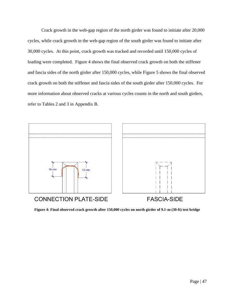
Page | 47

Crack growth in the web-gap region of the north girder was found to initiate after 20,000

cycles, while crack growth in the web-gap region of the south girder was found to initiate after

30,000 cycles. At this point, crack growth was tracked and recorded until 150,000 cycles of

loading were completed. Figure 4 shows the final observed crack growth on both the stiffener

and fascia sides of the north girder after 150,000 cycles, while Figure 5 shows the final observed

crack growth on both the stiffener and fascia sides of the south girder after 150,000 cycles. For

more information about observed cracks at various cycles counts in the north and south girders,

refer to Tables 2 and 3 in Appendix B.

Figure 4: Final observed crack growth after 150,000 cycles on north girder of 9.1-m (30-ft) test bridge

Page | 48

Figure 5: Final observed crack growth after 150,000 cycles on south girder of 9.1-m (30-ft) test bridge

As shown in the figure, cracks propagated around the connection plate-to-web weld toe in

both the north and south girders of the bridge. In each case, the specific crack path was fairly

complex. In the north girder, the crack initiated in the toe of the weld and propagated through

the weld until it reached the web on either side of the connection plate. On both sides of the

connection plate, the crack turned to start to propagate along the interface between the web and

the weld. These cracks were referred to as vertical cracks in observations. In the final

observation, the west vertical crack on the north girder had progressed along the interface 18-mm

(11/16-in.) from the weld toe and the east vertical crack on the north girder had progressed 19-

mm (3/4-in.) from the weld toe. No cracks were observed on the fascia side of the connection

plate on the north girder. In the south girder, cracking also initiated in the toe of the weld and

propagated through the weld until it reached the web on either side of the connection plate.

Cracking then propagated along the interface between the weld and the web until reaching 25-

mm (1-in.) from the weld toe. At this point, the crack branched on either side of the connection

plate. One branch of the crack continued to follow the interface between the weld and the web.

Page | 49

The total propagation path along this interface was referred to as vertical cracks in observations.

The other branch of the crack propagated horizontally into the web, and was referred to as spider

cracking in observations. On the west side of the connection plate on the south girder, the

vertical crack had progressed to 35-mm (1 3/8-in.) from the weld toe and the spider crack had

progressed to 6-mm (1/4-in.) from the edge of the weld. On the east side of the connection plate,

the vertical crack had progressed to 32-mm (1 1/4-in.) from the weld toe and the spider crack had

progressed to 10-mm (3/8-in.) from the edge of the weld. A 25-mm (1-in.) horizontal crack was

also observed on the fascia side of the connection plate directly opposite from where the cracks

had branched on the connection plate side.

In addition to tracking crack growth, deformation data was also collected on the test

bridge via LVDTs and strain gages. LVDTs were utilized to measure horizontal deflection of

both the north and south girders, with three LVDTs placed on the fascia side of both girders at

mid-span. One LVDT was placed at the center of the bottom flange of each girder, a second was

placed in the web 541-mm (21.3-in.) from the bottom of the girder, and a third was placed in the

top web-gap 872-mm (34.3-in.) from the bottom of the girder. Strain gages were also attached

near the connection plates of the webs on both the north and south girders. Four strain gages

were placed on the connection plate-side of each girder, while four strain gages were also placed

on the fascia side. Figure 6 shows the exact placement of the strain gages on the webs for both

girders. Gage placements were mirror images of each other on the north and south girders. All

of the gages were oriented in the vertical direction, and thus recorded vertical strain. The LVDT

and strain gage data was collected during two separate 355.9-kN (80-kip) static load tests on the

bridge. The first static test was conducted before any fatigue cycling was initiated, while the

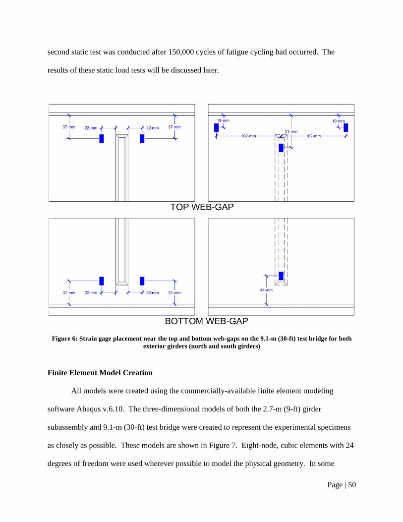
Page | 50

second static test was conducted after 150,000 cycles of fatigue cycling had occurred. The

results of these static load tests will be discussed later.

Figure 6: Strain gage placement near the top and bottom web-gaps on the 9.1-m (30-ft) test bridge for both

exterior girders (north and south girders)

Finite Element Model Creation

All models were created using the commercially-available finite element modeling

software Abaqus v.6.10. The three-dimensional models of both the 2.7-m (9-ft) girder

subassembly and 9.1-m (30-ft) test bridge were created to represent the experimental specimens

as closely as possible. These models are shown in Figure 7. Eight-node, cubic elements with 24

degrees of freedom were used wherever possible to model the physical geometry. In some

Page | 51

instances, four-node, tetrahedral elements with 12 degrees of freedom were utilized to conform

to special geometric aspects of the set-up. Fillet welds were modeled as right triangle cross-

sections with steel properties, and tie constraints were used to connect the fillet welds to the

surfaces they were joining together. Additionally, surfaces in the model expected to make

contact with one another were assigned interaction properties with a coefficient of friction of

0.35 to simulate hard contact. In the 2.7-m (9-ft) girder subassembly, elements in the web-gap

region were modeled as 3-mm x 3-mm x 3-mm (0.1-in. x 0.1-in. x 0.1-in.) eight-node cubic

elements. In the model of the 9.1-m (30-ft) half-scale bridge, elements in the web-gap were

modeled as 2-mm x 2-mm x 2-mm (1/16-in. x 1/16-in. x 1/16-in.) eight-node cubic elements.

The web-gap elements were sized as such because those values were the smallest observed

increment of crack growth during experimental observations of the specimens respectively.

Figure 7 shows the finite element models of both of these specimens.

Each part in the finite element models was assigned material properties. All steel

sections and welds in the both set-ups were modeled as isotropic, linear elastic materials with an

elastic modulus of 200,000-MPa (29,000-ksi) and a Poisson’s ratio of 0.3. The laboratory floor

in the 2.7-m (9-ft) girder subassembly and the concrete deck in the half-scale bridge were

modeled as concrete. The concrete sections were considered to be isotropic, linear elastic

material with an elastic modulus of 27,780-MPa (4,030-ksi) and a Poisson’s ratio of 0.2. To

simulate composite action in the model of the test bridge, the concrete deck was constrained to

the top flanges of the three girders along their entire length.

Page | 52

(a) (b)

Figure 7: Finite element models of (a) 2.7-m (9-ft) girder subassembly and (b) 9.1-m (30-ft) test bridge

Accurately Modeling Cracks

An examination of experimental test data from the 9.1-m (30-ft) test bridge in both

cracked and un-cracked states quickly showed that the presence of cracks created a different

localized stress state in the web-gap region than experienced in the un-cracked state. Table 1

presents the strains in the web of the north girder in the 9.1-m (30-ft) test bridge in un-cracked

and cracked states, while Table 2 presents the strains in the web of the south girder. At the strain

gages in the top web-gaps of the connection plate sides of both the north and south girders (strain

gages labeled NS-T-UE and NS-T-UW in the north girder; strain gages labeled SN-T-UE and

SN-T-UW in the south girder), a significant change can be noted in the measured values after

cracking occured. The other strain gages also exhibited changes in measured values. These

changes in strain response imply that finite element models that are intended to determine the

likelihood of future cracking or the effectiveness of fatigue retrofits must simulate cracking that

occurs in the web-gap region to be accurate. The fatigue cracks in the web-gap region of the test

bridge occurred near the connection plate-to-web weld. Since a weld already represents a

physical discontinuity, it can be difficult to portray a crack in the same vicinity because a crack is

Page | 53

also a discontinuity. Subsequently, these cracks may be difficult to model accurately. This

section will explore a few different methods for modeling stiffener-to-web weld cracks caused

by distortion-induced fatigue and will assess their accuracy.

Table 1: Vertical web strains (με) in north girder for un-cracked and cracked states

State/Gage NN-B-SC NN-T-SC NN-T-LE NN-T-LW NS-B-UE NS-B-UW NS-T-UE NS-T-UW

Un-Cracked -113 -962 237 231 -17 -22 468 377

Cracked -101 -980 206 177 -24 -28 162 70

Change 12 -18 -31 -54 -7 -6 -306 -307

Table 2: Vertical web strains (με) in south girder for un-cracked and cracked states

State/Gage SS-B-SC SS-T-SC SS-T-LE SS-T-LW SN-B-UE SN-B-UW SN-T-UE SN-T-UW

Un-Cracked -91 -1119 241 284 -28 -66 694 742

Cracked -90 -327 -848 N/A -36 -69 -60 -158

Change 1 792 -1089 N/A -9 -3 -754 -900

To assess the accuracy of various methods for modeling fatigue cracks around the

connection plate-to-web weld, finite element models implementing each method for modeling

the cracks were compared with experimental data from the 9.1-m (30-ft) test bridge. As

mentioned previously, 356-kN (80-kip) static tests were conducted when the bridge was in an

un-cracked state before fatigue cycling had commenced, and again when the bridge was in a

cracked state after 150,000 fatigue cycles had been accumulated. Data was recorded using three

LVDTs and eight strain gages in both the north and south girders for both tests, and the

differences in the recorded values from the cracked and un-cracked states were computed. These

differences were compared to finite element modeling results that also computed the differences

in strains and deflections between cracked and un-cracked states. The cracked state of the bridge

at 150,000 cycles was simulated with cracks modeled using the Extended Finite Element Method

within ABAQUS.

Page | 54

The Extended Finite Element Method, or XFEM, is a variation of the traditional finite

element method in which cracks can be simulated without having to conform to the finite

element mesh. The method was first introduced in 1999 (Moes et. al. 1999) and first

implemented within Abaqus v.6.9. Using XFEM, cracks can be modeled as cutting through the

middle of an element in a finite element mesh, which is accomplished by the addition of

discontinuous functions to the finite element solution so that elements can be detected as having

been cut by a crack or a crack tip. Thus, three distinct sets of nodes are used to approximate a

cracked model in XFEM solutions (Yazid et. al. 2009). These node sets are as follows:

(1) All nodes in the model domain

(2) Nodes whose shape function support is intersected by a crack

(3) Nodes whose shape function support contains the crack front.

In Abaqus v.6.10, cracks modeled using XFEM are created either by placing linear one-

dimensional sections within the framework of a shell model or by placing planar shell sections

within the framework of a three-dimensional solid model to simulate the discontinuity. Abaqus

v.6.10 detects which elements are completely cut by the simulated cracks and which elements are

cut by the crack tip. Since the solutions of the discontinuous functions applied to node sets (2)

and (3) are dependent on the distance of specific nodes from the discontinuity, Abaqus v.6.10

employs an algorithm to compute the distance to nodes in cracked elements. This method of

implementation allows for the geometry of the observed cracks along the stiffener-to-web weld

to be simulated with as much detail as desired. However, the literature has not addressed

whether this enhanced level of detail improves the accuracy of the finite element solution. Thus,

three different levels of crack detail around the stiffener-to-web weld were employed in this

Page | 55

study. These different levels of detail will be referred to as “Simple,” “Detailed Through-

Thickness,” and “Detailed Partial Thickness,” each described in the following discussions.

Simple XFEM Cracks

The first level of crack detail studied in the finite element models was termed “Simple.”

In this modeling approach, the general horseshoe shape of the connection plate-to-web weld

crack was simulated as having occurred in the web only. In both the north and south girders, the

parts of the cracks that had propagated through the weld toe were instead simulated as having

propagated around the outside of the weld toe at a distance of 0.6-mm (0.025-in.) from the toe of

the weld and were simulated as being through-thickness (extending through the full thickness of

the web). The vertical legs of the cracks were also simulated at a distance of 0.6-mm (0.025-in.)

from the edge of the weld and were through-thickness. It should be noted that these cracks were

placed at a very small distance from the toe of the weld instead of being placed directly along the

edge because the XFEM algorithm within Abaqus v.6.10 does not consistently simulate a crack

in the same manner when it is located along an interface. Additionally, another drawback of the

XFEM framework within Abaqus v.6.10 is that a continuous crack can only be simulated in a

single part instance. Thus, by simulating the cracks through the web only, it was possible to

model these cracks as one continuous through-thickness crack. These cracks were modeled as

through-thickness because it was impossible to tell through observation to what depth any of the

cracks had penetrated into the web thickness. Therefore, a weakness of this modeling approach

was that the modeled crack did not accurately portray the observed cracks on the fascia side of

the girders.

Page | 56

The spider cracks on either side of the connection plate were also modeled as through-

thickness based upon the experimental observations made on the connection plate side of the

girders. However, XFEM only allows for one crack to cut the framework of a given element,

therefore the spider cracks could not be simulated as having branched off from the main

horseshoe-shaped crack. Thus, spider cracks were modeled as occurring at a distance equal to a

single 1.6-mm (1/16-in.) element offset from the horseshoe-shaped crack on either side of the

stiffener. The obvious drawback of this was the likely stress concentration in that element gap.

Figure 8 and Figure 9 show how the cracks were modeled for the “Simple” modeling approach

on the north and south girders respectively.

Figure 8: “Simple” modeling approach for cracks observed after 150,000 cycles on north girder

Page | 57

Figure 9: “Simple” modeling approach for cracks observed after 150,000 cycles on south girder

Detailed Through-Thickness XFEM Cracks

The second modeling approach examined was termed “Detailed Through-Thickness.” In

this approach, the cracks observed as occurring through the weld toes were actually simulated in

the weld toes of the model. The drawback of modeling cracks at this level of detail was that the

connection plate-to-web welds were modeled as a separate part instance from the web, thus

meaning that the cracks simulated through the weld could not be continuous with the cracks

simulated in the web. Thus, these were modeled as separate cracks parallel to the interface

between the stiffener and the weld and offset by 0.6-mm (0.025-in.). As a result, the weld cracks

terminated at the interface between the weld and the web a distance of 9.5-mm (3/8-in.) from the

weld toe. This location marked the top of a U-shaped crack modeled through the web-thickness

in order to simulate the vertical cracks. The spider cracks were modeled as propagating from the

corner of this U-shape on either side of the connection plate and were once again offset by a

single 1.6-mm (1/16-in.) element. The cracks modeled using this level of detail more closely

resembled the experimental observations from the fascia sides of the girders than the “Simple”

Page | 58

level of detail, however they still did not match experimental observations perfectly, since cracks

were all simulated as through-thickness. Figure 10 and Figure 11 show how the cracks were

modeled for the “Detailed Through-Thickness” modeling approach on the north and south

girders respectively.

Figure 10: “Detailed Through-Thickness” modeling approach for cracks observed after 150,000 cycles on

north girder

Figure 11: “Detailed Through-Thickness” modeling approach for cracks observed after 150,000 cycles on

south girder

Page | 59

Detailed Partial-Thickness XFEM Cracks

The final level of crack modeling detail examined in the finite element model was termed

“Detailed Partial-Thickness.” The cracks modeled using this level of detail were modeled in a

way to almost perfectly match the experimental observations made on both the connection plate

and fascia sides of the girders. The cracks through the weld toes were modeled in the same

manner as those in the “Detailed Through-Thickness” level of detail, and cracks on the

connection plate sides of the webs were also modeled in the same manner. However, when

cracks on the connection plate sides of the webs were not observed as progressing to through-

thickness on the fascia sides in the experimental observations, these cracks were only modeled

half the distance through the web-thickness. This enabled the cracks on the fascia sides of the

webs to be matched almost perfectly. However, the single 1.6-mm (1/16-in.) element offset was

maintained between the spider cracks and where they branched from the vertical cracks. The

drawback of modeling the cracks using this technique remains with the fact that the actual crack

depth was still unknown. Thus, simulating partial-thickness cracks as being half the thickness

through the web was still a significant assumption. Figure 12 and Figure 13 show how the

cracks were modeled for the “Detailed Partial-Thickness” level of detail for both the north and

south girders respectively.

Page | 60

Figure 12: “Detailed Partial-Thickness” modeling approach for cracks observed after 150,000 cycles on

north girder

Figure 13: “Detailed Partial-Thickness” modeling approach for cracks observed after 150,000 cycles on

south girder

Page | 61

Comparison with Experimental Results

A finite element simulation of the 9.1-m (30-ft) test bridge in its un-cracked state at zero

completed cycles was conducted and compared against experimental results. This was done to

establish a baseline for the comparative study of the different methods of modeling web-gap

cracks. Vertical strains, ε22, were recorded at eight locations near the top and bottom web-gaps

on both the north and south girders. The comparison between experimental and finite element

results at these locations is shown in Table 3 for the north girder and Table 4 for the south girder.

Additionally, out-of-plane displacements measured by LVDTs at three locations on each girder

were recorded and compared with the finite element results. These results are shown in Figure

14, where positive values for out-of-plane displacement indicate displacement in the north

direction while negative values indicate displacement in the south direction.

Table 3: Comparison between vertical strains (με) in the experimental and finite element results

for un-cracked north girder

Set/Gage NN-B-SC NN-T-SC NN-T-LE NN-T-LW NS-B-UE NS-B-UW NS-T-UE NS-T-UW

Experimental -113 -962 237 231 -17 -22 468 377

FE Model -101 -683 223 98 147 114 556 553

Table 4: Comparison between vertical strains (με) in the experimental and finite element results

for un-cracked south girder

Set/Gage SS-B-SC SS-T-SC SS-T-LE SS-T-LW SN-B-UE SN-B-UW SN-T-UE SN-T-UW

Experimental -90 -1119 241 284 -28 -65 694 742

FE Model -98 -728 179 219 143 122 589 599

Page | 62

Figure 14: Comparison between experimental and finite element out-of-plane displacement results

It was expected that the finite element model results would not perfectly match the

experimental results and it was not a goal of this investigation to accomplish this. However, the

finite element model did capture the out-of-plane deformation shape of the girders correctly,

even if the results did not match the experimental findings perfectly. Additionally, reasonable

alignment was noted as occurring between the vertical strains from the finite element model and

the experimental vertical strains. Two strain gage locations where finite element model results

differed significantly from the experimental results were the strain gages labeled NN-T-SC and

SS-T-SC. These strain gages were mirrors of each other on the fascia sides of both the north and

south girders directly opposite the top of the connection plates. However, throughout

experimental testing, it was observed that the results recorded at these strain gages were

inconsistent, and, when the web-gap cracks progressed to through-thickness, they were within

13-mm (1/2-in.) of the gages. Therefore, the reliability of those two gage readings was not very

high.

-0.03 -0.015 0 0.015 0.03

0

5

10

15

20

25

30

35

0

100

200

300

400

500

600

700

800

900

1000

-0.762 -0.381 0 0.381 0.762

Out-of-Plane Displacement (in.)

Ve

rtic

al P

osi

tio

n o

n G

ird

er

(in

.)

Ve

rtic

al P

osi

tio

n o

n G

ird

er

(mm

)

Out-of-Plane Displacement (mm)

Exp. South FE South Exp. North FE North

Page | 63

With this starting point in mind, finite element models with cracks created using

“Simple,” “Detailed Through-Thickness,” and “Detailed Partial-Thickness” methods in XFEM

were examined under 356-kN (80-kip) static loads and then compared with experimental data

obtained under the same load. To eliminate discrepancies in the un-cracked state, change in

vertical strain, Δε22, at the eight strain gages in both girders was considered instead of just the

magnitudes. Thus, with the method of modeling the cracks being the only variable in the finite

element models and the actual cracks being the only variable in the experimental testing, the

finite element results could be adequately compared with the experimental results. Table 5

shows the comparison of the finite element modeling results with the experimental data in the

north girder while Table 6 shows the comparison of the results in the south girder.

Table 5: Comparison of Δε22 (με) for various XFEM methods for modeling web-gap cracks with experimental

results in north girder

Method/Gage NN-B-SC NN-T-SC NN-T-LE NN-T-LW NS-B-UE NS-B-UW NS-T-UE NS-T-UW

Experimental 11.73 -17.75 -30.84 -53.86 -6.63 -6.25 -306.25 -307.00

Simple 2.8 699.78 19.97 80.44 -13.33 19.99 -406.77 -314.21

Detailed-TT -0.95 716.66 30.87 93.41 -2.33 0.36 -408.66 -383.92

Detailed-PT -0.24 -207.16 27.58 88.8 -3.85 -1.51 -292.47 -273.45

Table 6: Comparison of Δε22 (με) for various XFEM methods for modeling web-gap cracks with experimental

results in south girder

Method/Gage SS-B-SC SS-T-SC SS-T-LE SS-T-LW SN-B-UE SN-B-UW SN-T-UE SN-T-UW

Experimental 0.26 792.45 -1088.79 N/A -7.75 -3.18 -753.75 -899.75

Simple -9.54 858 69.57 N/A 23.62 16.51 -907.58 -968.68

Detailed-TT -21.8 687.52 34.23 N/A 8.66 4.52 -464.52 -559.28

Detailed-PT -4.1 794.39 37.51 N/A 9.61 5.67 -459.74 -519.46

The data show varying levels of agreement for each modeling technique at different

strain gages. As previously mentioned, strain gages labeled NN-T-SC and SS-T-SC produced

inconsistent experimental results due to their proximity to the through-thickness crack.

Page | 64

Additionally, two other strain gages on the fascia side of the south girder, gages SS-T-LE and

SS-T-LW, also produced inconsistent results once cracks had initiated, with gage SS-T-LW

ceasing to record data at all. For the remaining strain gages, the accuracy of each method of

modeling the cracks was judged based on the strain gradients at each location. Figures of the

vertical strain contours and the stress contours at each strain gage location can be found in

Appendix B. Based on observations of these contours, the strain gages in the top web-gaps on

the fascia sides of both girders, NN-T-SC, NN-T-LE, NN-T-LW, SS-T-SC, SS-T-LE, and SS-T-

LW, were all located in areas of high gradient. Strain gages in the top web-gaps on the

connection plate sides of both girders, NS-T-UE, NS-T-UW, SN-T-UE, and SN-T-UW, were all

located in areas of moderate gradient. Finally, all of the strain gages in the bottom web-gaps,

NN-B-SC, NS-B-UE, NS-B-UW, SS-B-SC, SN-B-UE, and SN-B-UW, were located in areas of

low gradient. It should be noted that the gradients were fairly consistent across the models with

the different methods of modeling the cracks.

Although the gages were located in areas of moderate gradient, common sense would

hold that strain gages in the top web-gaps on the stiffener sides of the girders were likely more

affected by crack modeling technique than any of the gages in the bottom web-gap. Therefore, it

was not surprising that the largest difference between any Δε22 in the bottom web-gaps of the

finite element models was 21.5 με and that the largest difference from the experimental values

was 31.4 με. However, the four gages in the top web-gap on the connection plate sides of the

girders were more sensitive to crack modeling technique and were more useful in assessing the

crack modeling technique. On the north girder, the “Detailed Partial-Thickness” method had the

closest Δε22 to the experimental results at gage NS-T-UE and the “Simple” method had the

closest Δε22 to the experimental results at gage NS-T-UW, although the largest difference for any

Page | 65

of the methods was 102.4 με. On the south girder, the “Simple” method had the closest values

for Δε22 to the experimental results at both gages while the other two methods had larger

differences between the finite element and experimental results.

Based on a comparison of experimental data with finite element modeling results, the

closest alignment was achieved by using the “Simple” method. However, the differences

between each of the three methods analyzed were small, and none of the methods clearly

performed the best. Given that, it was concluded that there was no clear benefit to modeling

web-gap cracks with the “Detailed Through-Thickness” or “Detailed Partial-Thickness”

techniques. Thus, for the next section of this study, it was determined that modeling web-gap

cracks by the “Simple” method was sufficient, and all simulations discussed in the remainder of

this paper utilized this modeling technique.

Determining Paris’ Law Equations

Modeling cracks using the XFEM capabilities in Abaqus v.6.10 enabled more qualitative

information to be determined about distortion-induced fatigue because the mode I, II, and III

stress intensity factors, ΔKI, ΔKII, and ΔKIII, could be determined. A stress intensity factor

describes the likelihood of crack extension occurring ahead of a crack tip. ΔKI, ΔKII, and ΔKIII

represent the likelihood for each mechanism of crack opening, with ΔKI representing tensile

crack opening, ΔKII representing in-plane shear crack opening, and ΔKIII representing out-of-

plane shear crack opening. For each XFEM crack studied, an interaction integral method was

employed to extract ΔKI, ΔKII, and ΔKIII (Shih and Asaro 1988). This interaction integral is given

by the following expression:

∫ (

)

(1)

Page | 66

where σijaux

is the auxiliary stress field, εijaux

is the auxiliary strain field, and uiaux

is the auxiliary

displacement field. It was automatically computed by Abaqus v.6.10, which then substituted the

definitions of the actual and auxiliary fields into Equation 1 to get an expression in terms of the

actual and auxiliary mode I, II, and III stress intensity factors:

( )

(2)

In order to determine ΔKI, ΔKIaux

is set to 1 while ΔKIIaux

and ΔKIIIaux

are set to 0 (Gosz 2005).

ΔKII and ΔKIII are likewise determined in the same manner.

Fatigue Crack Propagation Theory

To make qualitative observations about crack propagation in the web-gap region from

these finite element simulations, the theory of fatigue crack propagation must be understood.

Fatigue crack propagation occurs in three stages and can be generalized by the relationships

presented in Figure 15.

Figure 15: Logarithmic plot of the typical fatigue crack growth rate vs. stress intensity factor range

og𝑑𝑎

𝑑𝑁

og 𝐾

I II III

𝐾𝐶 𝐾𝑇𝐻

Page | 67

Figure 15 presents a logarithmic plot of the crack growth rate, da/dN, versus the stress

intensity factor range, ΔK. The threshold stress intensity factor, ΔKTH, separates Stage I crack

growth from Stage II, and the critical stress intensity factor, ΔKIC, separates Stage II crack

growth from Stage III. ΔKTH is dependent on the load ratio, R, and, and is given by Barsom and

Rolfe (Barsom and Rolfe 1999). For this study, R is 0.174 for the 2.7-m (9-ft) girder

subassembly and 0.1 for the 9.1-m (30-ft) test bridge. Therefore, ΔKTH is 6-MPa-m1/2

(5.5-ksi-

in1/2

) for the 2.7-m (9-ft) subassembly and 6-MPa-m1/2

(5.5-ksi-in1/2

) for the 9.1-m (30-ft) test

bridge. ΔKIC is the fracture toughness property of the material being used, and is taken as at least

82 MPa-m1/2

(75 ksi-in1/2

) (FHWA 2012).

Stage I crack growth indicates cracks that will only propagate on the microscopic level if

they propagate at all. This behavior is difficult to predict since any crack growth is shear driven

and interacts with the microstructure of the material during this stage. In Stage II crack growth,

fatigue cracks propagate due to macroscopic, tension-driven crack growth. This stage of fatigue

crack growth is actually predictable and can be modeled by Paris’ Law (Paris and Erdogan

1963). Paris’ law relates crack growth rate with the stress intensity factor range and is given by

Equation (3):

⁄ (3)

where A and m are constants that vary for different materials. On the logarithmic plot in Figure

15, this is a linear relationship. For stage II crack growth in ferrite-pearlite steel, the estimated

Paris’ Law is given by Barsom and Rolfe (Barsom and Rolfe 1999):

⁄ (4)

where a is in in. and ΔK is in ksi-in1/2

. It should be noted that this estimate is given as an upper-

bound equation applied to steels under a constant tensile stress state. The final stage of crack

Page | 68

growth is Stage III crack growth. In this stage, crack growth is unstable and the growth rates

may accelerate to the point where brittle fracture occurs.

Computing Paris’ Law Coefficients

Cracks in the web-gap regions of both the 2.7-m (9-ft) girder subassembly and the 9.1-m

(30-ft) test bridge progressed during fatigue cycling. The 2.7-m (9-ft) subassembly was

subjected to actuator loads from 3.6-kN (0.8-kip) to 20.5-kN (4.6-kip) for a load range of 16.9-

kN (3.8-kip). The 9.1-m (30-ft) test bridge was subjected to actuator loads from 26.7-kN (6-kip)

to 267-kN (60-kip) for a load range of 240.3-kN (54-kip). To simulate different points during

crack growth, static finite element simulations were conducted with the observed crack growth

modeled for particular points in time. The 2.7-m (9-ft) subassembly models were subjected to a

16.9-kN (3.8-kip) static load to simulate the range of one half cycle of loading, and the stress

intensity factors were computed for the various stages of crack growth. Likewise, the 9.1-m (30-

ft) bridge models were also subjected to a 240.3-kN (54-kip) static load, and the stress intensity

factors were once again computed at the various stages of crack growth.

By computing the mode I, mode II, and mode III stress intensity factors and then

converting them to an equivalent mode I stress intensity factor, the coefficients for Paris’ Law, A

and m, can be determined. ΔKI, ΔKII, and ΔKIII can be converted to a singular J-Integral value by

the following expression:

( )

(5)

where E is the elastic modulus, v is Poisson’s ratio, and G is the shear modulus (Sih and

Macdonald 1974, Sih and Cha 1974). Since linear-elastic behavior was assumed for steel in

these models, the J-Integral can be taken as the same as the strain energy release rate per unit

Page | 69

crack extension, G. Thus, the J-Integral can be related to an equivalent mode I stress intensity

factor by the following expression:

( )

(6)

Experimental observations of both the 2.7-m (9-ft) girder subassembly and the 9.1-m (30-

ft) test bridge were able to produce the rate of fatigue crack growth, da/dN, at any particular

cycle count. Likewise, the finite element simulations were able to produce the equivalent mode I

stress intensity factors, ΔKI,eq, at those same cycle counts. Taking the logarithm of both sets of

values and plotting log(ΔKI,eq) for all ΔKI,eq between ΔKTH and ΔKIC on the x-axis and log(da/dN)

on the y-axis enabled a line of fit to be applied to the data. The slope of this line of fit

represented the same value as the Paris’ Law coefficient m, while the y-intercept represented the

power of 10 to which the Paris’ Law coefficient A was taken.

For the 2.7-m (9-ft) girder subassembly, fatigue cracks propagated along both the

connection plate-to-web weld and the flange-to-web weld. Thus, the Paris’ Law coefficients

were determined for both major crack paths. Figure 16 shows the logarithmic plot of the crack

growth rate compared to the computed mode I stress intensity factors along the stiffener-to-web

weld for computed values of ΔKI,eq that fell between ΔKTH and ΔKIC. The line of fit applied to

this data resulted in the following Paris’ Law equation:

⁄ (7)


.

Page | 70

Figure 16: Logarithmic plot of crack growth rate vs. stress intensity factor range for the connection plate-to-

web weld crack on the 2.7-m (9-ft) girder subassembly

The equation for stage II crack growth at the connection plate-to-web weld compared very

closely with Equation (4), the estimated Paris’ Law for a ferrite-pearlite steel in a constant tensile

stress state. Both coefficients, A and m, were slightly larger than the expected values. This

would indicate that the driving mechanism behind fatigue crack growth along the connection

plate-to-web weld was predominantly tensile, although there was likely some contribution from

out-of-plane stresses as well, thus resulting in values slightly higher than those given by

Equation (4).

Figure 17 shows the same logarithmic plot for the horizontal crack that progressed along

the flange-to-web weld. The line of fit applied to the data resulted in the following Paris’ Law

equation:

⁄ (8)


.

1 10 100

-4.6

-4.4

-4.2

-4

-3.8

-3.6

-3.4

-3.2

-3

-2.8

-2.6

-6

-5.8

-5.6

-5.4

-5.2

-5

-4.8

-4.6

-4.4

-4.2

-4

1 10 100

ΔK, MPa-m^1/2

Log

(da/

dN

), m

m/c

ycle

Log

(da/

dN

), in

/cyc

le

ΔK, ksi-in^1/2

Page | 71

Figure 17: Logarithmic plot of crack growth rate vs. stress intensity factor range for the flange-to-web weld

crack on the 2.7-m (9-ft) girder subassembly

The equation for stage II crack growth for the flange-to-web weld was discernibly different than

Equation (4). The coefficient m was significantly different than the expected value for a constant

stress state. This would indicate that the driving mechanism behind fatigue crack growth along

the flange-to-web weld was mainly due to out-of-plane stresses. This would make sense given

that the crack tips would be removed from the high stress region in the web-gap, thus lowering

the tensile stress, and also because there was greater out-of-plane deformation for longer cracks,

thus increasing the out-of-plane stresses.

For the 9.1-m (30-ft) test bridge, cracks propagated along the connection plate-to-web

welds in both the north and south girders. Thus, separate Paris’ Law coefficients were

determined for each girder. Figure 18 shows the logarithmic plot of the crack growth rate

compared to the computed mode I stress intensity factors for the north girder. The line of fit

applied to this data resulted in the following Paris’ Law equation:

1 10 100

-4.6

-4.4

-4.2

-4

-3.8

-3.6

-3.4

-3.2

-3

-2.8

-2.6

-6

-5.8

-5.6

-5.4

-5.2

-5

-4.8

-4.6

-4.4

-4.2

-4

1 10 100

ΔK, MPa-m^1/2

Log

(da/

dN

), m

m/c

ycle

Log

(da/

dN

), in

/cyc

le

ΔK, ksi-in^1/2

Page | 72

⁄ (9)


.

Figure 18: Logarithmic plot of the crack growth rate vs. stress intensity factor range for the connection plate-

to-web weld crack on the north girder of the 9.1-m (30-ft) test bridge

The equation for stage II crack growth in the north girder was very different from Equation (4).

The coefficient m was more than double its value for an edge crack in a tensile specimen, while

the coefficient A was multiple powers smaller than its value for an edge crack in a tensile

specimen. This would indicate that there were other factors contributing to the crack growth rate

than stress since the computed stress intensity factors were largely unchanged at very different

growth rates.

Figure 19 shows the same logarithmic plot for the horizontal crack that progressed along

the flange-to-web weld. The line of fit applied to the data resulted in the following Paris’ Law

equation:

1 10 100

-4.6

-4.4

-4.2

-4

-3.8

-3.6

-3.4

-3.2

-3

-2.8

-2.6

-6

-5.8

-5.6

-5.4

-5.2

-5

-4.8

-4.6

-4.4

-4.2

-4

1 10 100

ΔK, MPa-m^1/2

Log

(da/

dN

), m

m/c

ycle

Log

(da/

dN

), in

/cyc

le

ΔK, ksi-in^1/2

Page | 73

⁄ (10)


.

Figure 19: Logarithmic plot of the crack growth rate vs. stress intensity factor range for the connection plate-

to-web crack on the south girder of the 9.1-m (30-ft) test bridge

The equation for stage II crack growth in the north girder compares favorably with Equation (4).

The coefficient m was only slightly larger while the coefficient A was only slightly smaller. This

would indicate that the fatigue crack growth in the south girder was very similar to edge crack

growth in a tensile specimen.

Conclusions

Only recently have finite element simulations of distortion-induced fatigue included a

level of detail including the cracks that occur in the web-gap regions of highway bridge girders.

The implementation of the Extended Finite Element Method (XFEM) has made it possible to

1 10 100

-4.6

-4.4

-4.2

-4

-3.8

-3.6

-3.4

-3.2

-3

-2.8

-2.6

-6

-5.8

-5.6

-5.4

-5.2

-5

-4.8

-4.6

-4.4

-4.2

-4

1 10 100

ΔK, MPa-m^1/2

Log

(da/

dN

), m

m/c

ycle

Log

(da/

dN

), in

/cyc

le

ΔK, ksi-in^1/2

Page | 74

model these cracks with very high levels of detail. In this study, finite element simulations were

conducted of a 9.1-m (30-ft) test bridge specimen with experimentally observed cracks. These

cracks were modeled with various levels of detail using XFEM, and the subsequent finite

element models were compared with experimental results to determine the most accurate level of

detail. The following conclusions were reached in this comparative study:

(1) The experimental strain gage and LVDT data significantly changed between the

un-cracked and cracked states of the bridge girders in the specimen. Based on

this, a significant loss in accuracy may be expected in finite element simulations

that do not model cracked geometry when the focus is on web-gap performance

under distortion-induced fatigue.

(2) Experimentally recorded strains in regions of high strain gradient were found to

be unreliable.

(3) All three crack modeling levels of detail were able to accurately compute

strains in regions of low strain gradient with a reasonable level of accuracy based

on comparison to experimental data.

(4) There was no increase in modeling accuracy for web-gap cracks modeled through

the connection plate-to-web weld or for web-gap cracks modeled as partial

thickness.

Based on these conclusions, web-gap cracks were modeled at various cycle counts for

both a 2.7-m (9-ft) girder subassembly and a 9.1-m (30-ft) test bridge. At the stiffener-to-web

weld, these cracks were modeled around the weld toe through the thickness of the web only. The

following conclusions were reached from these models:

Page | 75

(5) A method was established for determining Paris’ Law equations for observed

crack growth along welds.

(6) The Paris’ Law equations for each experimentally observed crack path describe

the fatigue crack growth behavior for any stress state. Therefore, it can be

determined what effect the changing of applied stress has on each fatigue crack.

Acknowledgements

The authors are grateful for support from the Kansas Department of Transportation

(KDOT) and the University of Kansas Transportation Research Institute (KU TRI). The authors

would also like to appreciatively acknowledge support provided though Pooled Fund Study TPF-

5(189), which includes the following participating State DOTs: Kansas, California, Iowa,

Illinois, New Jersey, New York, Oregon, Pennsylvania, Tennessee, Wisconsin, and Wyoming, as

well as the Federal Highway Administration.

References

[1] Adams, C. A. (2010). “Finite Element Study on Bridge Details Susceptible to Distoriton-Induced Fatigue,”

thesis, submitted to the University of Kansas in partial fulfillment of requirements for the degree of Master

of Science in Civil Engineering.

[2] Alemdar, F., et. al. (2013). “Repairing Distortion-Induced Fatigue Cracks in Steel Bridge Girders using Angle-

with-Plate Retrofit Technique: Part II: Computer Simulations.” Journal of Structural Engineering, In Press.

[3] Barsom, John M., and Rolfe, Stanley T. (1999). Fracture and Fatigue Control in Structures: Application of

Fracture Mechanics, 3rd

Edition. American Society for Testing and Materials, West Conshohocken, PA.

[4] Berglund, E. and Schultz, A. E. (2001). “Analysis Tools and Rapid Screening Data for Assessing Distortional

Fatigue in Steel Bridge Girders,” Minnesota Department of Transportation, Final Report 2002-06.

[5] Berglund, E. and Schultz, A. E. (2006). “Girder Differential Deflection and Distortion-Induced Fatigue in

Skewed Steel Bridges,” Journal of Bridge Engineering, vol. 11, pp. 169-177.

[6] FHWA (2012). Steel Bridge Design Handbook: Bridge Steels and Their Mechanical Properties. Federal

Highway Administration, Washington, DC.

Page | 76

[7] Gosz, M. (2005). “An Interaction Integral Method for Computation of T-Stress Along the Fronts of General

Non-Planar Cracks in Three-Dimensions.” 11th

International Conference on Fracture Proceedings, Turin,

Italy.

[8] Hartman, A., et. al. (2010). “Effects of lateral bracing placement on distortion-induced fatigue in steel bridges,”

Transportation Research Record, no. 2200, pp. 62-68.

[9] Hassel, H., et. al. (2010). “Distortion-induced fatigue in steel bridges: causes, parameters, and fixes,”

Proceedings of the ASCE/SEI Structures Congress, Orlando, FL, May 12-15, 2010.

[10] Hassel, H. et. al. (2012). “Parametric analysis of cross-frame layout on distortion-induced fatigue in skewed

steel bridges,” Journal of Bridge Engineering, In Press.

[11] Jajich, D., et. al. (2000). “Distortion-Induced Fatigue in Multi-Girder Steel Bridges,” Minnesota Department of

Transportation, Final Report 2000-16.

[12] Jajich, D. and Schultz, A. E. (2003). “Measurement and Analysis of Distortion-Induced Fatigue in Multigirder

Steel Bridges,” Journal of Bridge Engineering, vol. 8, pp. 84-91.

[13] Li, H. and Schultz, A. E. (2005). “Analysis of Girder Differential Deflection and Web Gap Stress for Rapid

Assessment of Distortional Fatigue in Multi-Girder Steel Bridges,” Minnesota Department of

Transportation, Final Report 2005-38.

[14] Moes, N., et. al. (1999). “A finite element method for crack growth without remeshing.” International Journal

for Numerical Methods in Engineering, vol. 46, pp. 131-150.

[15] Paris, P., and Erdogan, F. (1963). “A critical analysis of crack propagation laws.” Journal of Basic Engineering,

vol. 85, no. 4, pp. 528-533.

[16] Richardson, T., et. al. (2012). “Retrofit measures for distortion-induced fatigue,” Modern Steel Construction,

American Institute of Steel Construction, vol. 52, no. 4, pp. 32-34.

[17] Richardson, T., et. al. (2012). “Evaluation of the performance of retrofit measures for distortion-induced fatigue

using finite element analysis,” Proceedings of the National Steel Bridge Alliance World Steel Bridge

Symposium, Chicago, IL.

[18] Roddis, W. M. K., and Zhao, Y. (2003). “Finite-Element Analysis of Steel Bridge Distortion-Induced Fatigue,”

Journal of Bridge Engineering, vol. 8, pp. 259-266.

[19] Severtson, B., et. al. (2004). “Rapid Assessment of Distortional Stresses in Multi-Girder Steel Bridges,”

Minnesota Department of Transportation, Final Report 2004-48.

[20] Shih, C. F., and Asaro, R. J. (1988). “Elastic-Plastic Analysis of Cracks on Bimaterial Interaces: Part I—Small

Scale Yielding.” Journal of Applied Mechanics, vol. 55, no. 2, pp. 299-316.

[21] Sih, G. C., and Cha, B. C. K. (1974). “A fracture criterion for three-dimensional crack problems.” Engineering

Fracture Mechanics, vol. 6, no. 4, pp. 699-723.

[22] Sih, G. C., and Macdonald, B. (1974). “Fracture mechanics applied to engineering problems—strain energy

density fracture criterion.” Engineering Fracture Mechanics, vol. 6, no. 2, pp. 361-386.

[23] Yazid, A., et. al. (2009). “A state-of-the-art review of the X-FEM for computational fracture mechanics.”

Applied Mathematical Modeling, vol. 33, pp. 4269-4282.

[24] Zhao, Y. and Roddis, W. M. K. (2004). “Fatigue Prone Steel Bridge Details: Investigation and Recommended

Repairs,” Final Report to KDOT, KU-99-2.

Page | 77

[25] Zhao, Y. and Roddis, W. M. K. (2000). “Fatigue crack investigation for the Arkansas River Bridge in

Hutchinson, Kansas,” Construction and Building Materials, vol. 14, pp. 287-295.

[26] Zhao, Y. and Roddis, W. M. K. (2003). “Finite element study of distortion-induced fatigue in welded steel

bridges,” Transportation Research Record, no. 1845, pp. 57-65.

[27] Zhao, Y. and Roddis, W. M. K. (2007). “Fatigue Behavior and Retrofit Investigation of Distortion-Induced

Web Gap Cracking,” Journal of Bridge Engineering, vol. 12, pp. 737-745.

Page | 78

Appendix A: Using the Extended Finite Element Method (XFEM) to

Model Cracks in ABAQUS

The Extended Finite Element Method (XFEM) implementation within Abaqus v.6.10 has

enabled an efficient way for cracks to be simulated in bridge girders. The most significant aspect

of XFEM cracks are that they can be modeled independent of the finite element mesh.

Therefore, cracks can be modeled with great detail and can be changed without having to re-

mesh the model. This section will provide step-by-step instruction for how to model cracks via

XFEM in the Abaqus v.6.10 interface.

Page | 79

(1) Create the Part to be cracked and Mesh the Part to be cracked as normal.

Page | 80

(2) For a crack going into a three-dimensional model, create the desired crack geometry as a

three-dimensional Shell Part. This Part does not need to be assigned a Mesh or Section.

Input the Crack Part into the assembly in the desired location.

Page | 81

(3) Go to the Interaction module. Click on the pull-down menu labeled “Special,” scroll

down to the option labeled “Crack,” and select “Create.”

The resulting menu will prompt for the selection of “Contour Integral” or “XFEM” as

well as the input for the name of the crack. Input the desired crack name and select

“XFEM.”

Page | 82

(4) The subsequent prompt will ask the user to select the crack domain. The default selection

method is a “single instance,” however, this can be changed to “geometric cells.” The

“geometric cells” selection is ideal in larger models since it enables only sections of an

instance to be selected as the crack domain, thus creating a smaller computation than the

selection of a whole instance. There is a drawback to modeling cracks by XFEM in this

step because only one instance or sections within one instance can be selected for the

crack domain. Once the selection method is determined, click on the desired section to

be the domain. It will highlight in red. Select “Done.”

Page | 83

(5) At this point, the “Edit Crack” box will appear. The already selected crack domain

appears next to the label “Region.” This can be edited at any time. The rest of the box

contains different options for the XFEM crack. The first of these options is a box to

“Allow crack growth.” The default selection has this box checked. Allowing crack

growth to occur with XFEM is a time consuming modeling procedure that has only been

proven accurate for simple stress states such as a tensile specimen in quasi-static loading.

If running a static model, uncheck the “Allow crack growth” box.

(6) The next option down in the “Edit Crack” box is the “Crack location” prompt. No crack

location should be specified, so this must be done now. Click the “Select” box next to

the “Crack location” prompt.

Page | 84

(7) At this point, a two-dimensional surface must be selected within the already specified

crack domain to represent the crack. Select the Shell Instance in the Assembly that has

been created to represent the crack geometry. If selecting multiple surfaces to represent

the crack, make sure none of the surfaces intersect. One of the major weaknesses of

XFEM is that it cannot compute intersecting or branched cracks. Surfaces that terminate

at a mutual edge are fine, however the resulting angle between the surfaces must be at

least 90°. Once the crack surface is selected, it will highlight in pink. The crack domain

should still be highlighted in red. Select “Done.”

Page | 85

(8) The “Edit Crack” box will return with the “Region” and “Crack location” options now

complete. The next option in the box is the “Enrichment radius.” The default selection is

“Analysis default,” which means that Abaqus will automatically compute the enrichment

radius. This option is fine. The other option is “Specify,” which allows the user to input

their desired enrichment radius. This option can only make things worse from “Analysis

default.”

(9) The final option in the “Edit Crack” box is the “Specify contact property” option. This

option is useful if there is a chance the crack surfaces would intersect. When selecting

this option, all of the created interaction properties will be available for selection in the

pull-down menu. Select the appropriate interaction property if choosing this option.

Please note, that the interaction property name must not contain any spaces or else the

model will abort when trying to run.

(10) If happy with all selections in the “Edit Crack” box, select “Ok.” The XFEM crack has

now been created and can be edited at any time by going to the “Special” pull-down,

selecting the “Crack” menu, and selecting the “Edit” menu.

Page | 86

(11) In order to obtain output data from the modeled XFEM crack, create a “History Output

Request” in the Load Step. The first option in the “Edit History Output Request” box is

selecting the domain for the output. The default is set to “Whole model,” however, this

can be changed to “Crack.”

In the “Domain” option, a sub-option will appear to select the particular crack of interest

to obtain output from. The next option is for the “Frequency” of output data to be

written. The default is set to “Every n increments.” This option can be changed to “Last

increment” in models that expect multiple increments to complete. The next option is the

“Number of contours” to be created. 5 should be sufficient to match linear-elastic

behavior between the finite element model and a physical specimen. The next option is

for the “Type” of contour integral. Select whatever appropriate, however, when selecting

“Stress intensity factors,” use the “Maximum tangential stress” crack initiation criterion.

If satisfied with the output selections, click “Ok.”

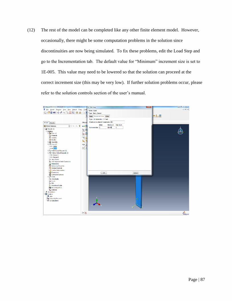
Page | 87

(12) The rest of the model can be completed like any other finite element model. However,

occasionally, there might be some computation problems in the solution since

discontinuities are now being simulated. To fix these problems, edit the Load Step and

go to the Incrementation tab. The default value for “Minimum” increment size is set to

1E-005. This value may need to be lowered so that the solution can proceed at the

correct increment size (this may be very low). If further solution problems occur, please

refer to the solution controls section of the user’s manual.

Page | 88

Appendix B: Supplemental Information for Part II

Introduction

In Part II, finite element simulations using the extended finite element method were

employed to determine the most accurate way to portray distortion-induced fatigue cracks and to

determine Paris’ Law equations for progressing cracks in experimental specimens. Information

used in obtaining some of the results was not mentioned for the sake of length concerns. This

appendix will provide such information associated with Part II as well as any additional

information that might be necessary to answer questions from peer reviews.

Crack Growth vs. Cycles

For both the 2.74-m (9-ft) subassembly and the 9.14-m (30-ft) bridge, crack growth in the

web-gap region was tracked during fatigue load cycling. The 2.74-m (9-ft) subassembly

experienced crack growth along both the stiffener-to-web weld and the flange-to-web weld while

being subjected to a load ranging from an upper-bound of 20.46-kN (4.6-kip) to a lower-bound

load of 3.56-kN (0.8-kip) for a load range of 16.90-kN (3.8-kip). The 9.14-m (30-ft) bridge

experienced crack growth in two separate girders but along the stiffener-to-web weld only while

being subjected to a load ranging from an upper-bound of 266.89-kN (60-kip) to a lower-bound

of 26.69-kN (6-kip) for a load range of 240.20-kN (54-kip). This section provides tables of the

complete recorded crack growth history during fatigue cycling. Table 1 shows all of the

observed crack growth in the 2.74-m (9-ft) subassembly, Table 2 shows all of the observed crack

growth in the north girder of the 9.14-m (30-ft) bridge, and Table 3 shows all of the observed

crack growth in the south girder of the 9.14-m (30-ft) bridge.

Page | 89

Table 1: Crack growth (in.) vs. number of cycles for 2.7-m (9-ft) girder subassembly

Cycles Toe Vertical-L Vertical-R Spider-L Spider-R Fascia Horiz.

0 0 0 0 0 0 0 0

13800 0 0 0 0 0 0 0

23700 0 0 0 0 0 0 0

44000 0 0 0 0 0 0 0

50000 0 0 0 0 0 0 0

60000 0 0 0 0 0 0 0

73000 0.4 0 0 0 0 0 0

99500 0.8 0 0 0 0 0 0

150000 0.8 1 1.1 0 0 0 0

165000 0.8 1 1.1 0 0 0 0

172000 0.8 1 1.1 0 0 0 0

182000 0.8 1 1.1 0 0 0 0

200000 0.8 1 1.1 0.1 0 0 0

230000 0.8 1 1.1 0.1 0 0 0

250000 0.8 1.8 2 0.3 0.3 0 0.2

270000 0.8 1.8 2 0.4 0.4 0 0.4

281000 0.8 1.8 2 0.5 0.5 0 1

310900 0.8 1.8 2 0.5 0.5 0 1

378900 0.8 1.8 2 0.5 0.5 0 2

394900 0.8 1.8 2 0.5 0.5 0 2

410900 0.8 1.8 2 0.5 0.5 0 2

431900 0.8 1.8 2 0.8 0.8 1 3

443900 0.8 1.8 2 0.8 0.8 1 3

462600 0.8 2 2.5 0.8 0.8 1.4 4

491700 0.8 2 2.5 0.8 0.8 1.4 4

507500 0.8 2 2.5 0.8 0.8 1.5 4

524400 0.8 2 2.5 0.8 0.8 1.6 4

554400 0.8 2 2.5 0.9 1 1.6 4.2

567200 0.8 2 2.5 0.9 1 1.8 4.2

618900 0.8 2 2.5 0.9 1 1.9 4.8

651900 0.8 2 2.5 0.9 1 1.9 5.2

678900 0.8 2 2.5 0.9 1 1.9 5.2

703900 0.8 2 2.5 0.9 1.1 1.9 5.6

727900 0.8 2.1 2.8 0.9 1.1 1.9 5.6

741900 0.8 2.1 2.8 0.9 1.1 1.9 5.8

765900 0.8 2.1 2.8 0.9 1.1 2 6

818900 0.8 2.1 2.8 0.9 1.3 2 6.4

837900 0.8 2.1 2.8 0.9 1.3 2 6.8

866900 0.8 2.1 2.8 0.9 1.3 2 7.2

888900 0.8 2.1 2.8 0.9 1.3 2 7.2

900900 0.8 2.1 2.9 0.9 1.3 2 7.6

918900 0.8 2.1 2.9 0.9 1.3 2 7.6

965900 0.8 2.1 2.9 0.9 1.3 2 7.6

977900 0.8 2.1 2.9 0.9 1.3 2 7.8

1028900 0.8 2.1 2.9 0.9 1.3 2 8

1040900 0.8 2.1 2.9 0.9 1.3 2 8.2

Page | 90

Table 2: Crack growth (in.) vs number of cycles for north girder of 9.1-m (30-ft) test bridge

Cycles Toe Vertical-W Spider-W Vertical-E Spider-E Fascia

0 0 0 0 0 0 0

15,000 3/4 0 0 0 0 0

20,000 3/4 1/2 0 0 0 0

30,000 3/4 9/16 0 7/16 0 0

35,000 3/4 5/8 0 5/8 0 0

40,000 3/4 5/8 0 5/8 0 0

45,000 3/4 5/8 0 5/8 0 0

50,000 3/4 5/8 0 5/8 0 0

55,000 3/4 5/8 0 5/8 0 0

60,000 3/4 11/16 0 5/8 0 0

65,000 3/4 11/16 0 11/16 0 0

70,000 3/4 11/16 0 11/16 0 0

75,000 3/4 11/16 0 11/16 0 0

90,000 3/4 11/16 0 3/4 0 0

105,000 3/4 11/16 0 3/4 0 0

120,000 3/4 11/16 0 3/4 0 0

135,000 3/4 11/16 0 3/4 0 0

150,000 3/4 11/16 0 3/4 0 0

Table 3: Crack growth (in.) vs number of cycles for south girder of 9.1-m (30-ft) test bridge

Cycles Toe Vertical-E Spider-E Vertical-W Spider-W Fascia

0 0 0 0 0 0 0

15,000 0 0 0 0 0 0

20,000 3/4 0 0 0 0 0

30,000 3/4 1/2 0 7/16 0 0

35,000 3/4 1/2 0 7/16 0 0

40,000 3/4 9/16 0 1/2 0 0

45,000 3/4 9/16 0 5/8 0 0

50,000 3/4 5/8 0 5/8 0 0

55,000 3/4 11/16 0 3/4 0 0

60,000 3/4 3/4 0 3/4 0 0

65,000 3/4 15/16 0 1 0 0

70,000 3/4 1 0 1 0 0

75,000 3/4 1 0 1 0 0

90,000 3/4 1 0 1 0 0

105,000 3/4 1 0 9/8 1/16 0

120,000 3/4 1 0 9/8 1/8 0

135,000 3/4 9/8 1/8 9/8 1/4 0*

150,000 3/4 11/8 1/4 5/4 3/8 1

Page | 91

Figure 1: Total horseshoe crack growth vs. number of cycles for the 2.7-m (9-ft) subassembly

Figure 2: Horizontal crack growth vs. number of cycles for the 2.7-m (9-ft) subassembly

y = 6.9499x - 33.197 R² = 0.961

0

50

100

150

200

250

0

1

2

3

4

5

6

7

8

9

10

0 1 2 3 4 5 6 7

Cra

ck L

en

gth

, 2a

(mm

)

Cra

ck L

en

gth

, 2a

(in

.)

Log(Cycles)

y = 12.949x - 69.974 R² = 0.9847

0

50

100

150

200

250

0

1

2

3

4

5

6

7

8

9

10

0 1 2 3 4 5 6 7 8

Cra

ck L

en

gth

, 2a

(mm

)

Cra

ck L

en

gth

, 2a

(in

.)

Log(Cycles)

Page | 92

Figure 3: Total horseshoe crack growth on north girder vs. number of cycles for 9.1-m (30-ft) test bridge

Figure 4: Total horseshoe crack growth on north girder vs. number of cycles for 9.1-m (30-ft) test bridge

y = 0.6832x - 1.9853 R² = 0.8703

0

20

40

60

80

100

0

0.5

1

1.5

2

2.5

3

3.5

4

0 1 2 3 4 5 6

Cra

ck L

en

gth

, 2a

(mm

)

Cra

ck L

en

gth

, 2a

(in

.)

Log (Cycles)

y = 2.7055x - 11.263 R² = 0.9306

0

20

40

60

80

100

0

0.5

1

1.5

2

2.5

3

3.5

4

0 1 2 3 4 5 6

Cra

ck L

en

gth

, 2a

(mm

)

Cra

ck L

en

gth

, 2a

(in

.)

Log (Cycles)

Page | 93

Stress and Strain Contour Plots

In finite element models of the 9.14-m (30-ft) bridge, three different XFEM methods of

modeling the web-gap cracks were employed. Vertical strains (ε22) from the finite element

simulations were compared with experimental data from strain gages placed in the webs of both

the north and south girders, and the most accurate method was determined. Part of the

assessment of the accuracy of these methods was based on the level of gradient in the vertical

strains (ε22) and the maximum principal stresses (σmax) at the gage locations. This section will

provide the contour plots in the web-gaps from the finite element simulation employing the

“Simple” method of modeling the web-gap cracks. The gradients in the different methods were

just about the same, thus the simulation with the “Simple” method for modeling the web-gap

cracks will serve as an example of the gradients in each web-gap. Figure 5 shows the range of

contour values for vertical strain and maximum principal stress used in the images in the rest of

this section.

(a) (b)

Figure 5: Contours for (a) Vertical Strain, ε22, and (b) Maximum Principal Stress, σmax (ksi)

Page | 94

Figure 6: Vertical strain (ε22) contours in top web-gap of the fascia side of the north girder

Figure 7: Vertical strain (ε22) contours in bottom web-gap of the fascia side of the north girder

NN-T-LE

NN-T-SC

NN-T-LW

NN-B-SC

Page | 95

Figure 8: Vertical strain (ε22) contours in top web-gap of the connection plate side of the north girder

Figure 9: Vertical strain (ε22) contours in bottom web-gap of the connection plate side of the north girder

NS-T-UW NS-T-UE

NS-B-UW NS-B-UE

Page | 96

Figure 10: Vertical strain (ε22) contours in top web-gap of the fascia side of the south girder

Figure 11: Vertical strain (ε22) contours in bottom web-gap of the fascia side of the south girder

SS-T-SC

SS-T-LW SS-T-LE

SS-B-SC

Page | 97

Figure 12: Vertical strain (ε22) contours in top web-gap of the connection plate side of the south girder

Figure 13: Vertical strain (ε22) contours in bottom web-gap of the connection plate side of the south girder

SN-T-UW SN-T-UE

SN-B-UW SN-B-UE

Page | 98

Figure 14: Maximum Principal Stress (σmax) Contours in Top Web-gap of the Fascia Side of the North Girder

Figure 15: Maximum Principal Stress (σmax) Contours in Bottom Web-gap of the Fascia Side of the North Girder

NN-T-SC

NN-T-LW NN-T-LE

NN-B-SC

Page | 99

Figure 16: Maximum Principal Stress (σmax) Contours in Top Web-gap of the Stiffener Side of the North Girder

Figure 17: Maximum Principal Stress (σmax) Contours in Bottom Web-gap of the Stiffener Side of the North Girder

NS-T-UE NS-T-UW

NS-B-UE NS-B-UW

Page | 100

Figure 18: Maximum Principal Stress (σmax) Contours in Top Web-gap of the Fascia Side of the South Girder

Figure 19: Maximum Principal Stress (σmax) Contours in Bottom Web-gap of the Fascia Side of the South Girder

SS-T-SC

SS-T-LE SS-T-LW

SS-B-SC

Page | 101

Figure 20: Maximum Principal Stress (σmax) Contours in Top Web-gap of the Stiffener Side of the South Girder

Figure 21: Maximum Principal Stress (σmax) Contours in Bottom Web-gap of the Stiffener Side of the South Girder

SN-T-UW SN-T-UE

SN-B-UW SN-B-UE

Page | 102

Appendix C: Converting Paris’ Law Equations into an S-N Diagram

Introduction

In Part II, a method to determine Paris’ Law coefficients was created to describe crack

growth in a 2.7-m (9-ft) girder subassembly and a 9.1-m (30-ft) test bridge. With these

coefficients applied to Paris’ Law for fatigue crack growth, the resulting equations could

describe the crack growth at a detail with any applied stress. However, to most bridge engineers,

Paris’ Law does not have much significance since it is hard to quantify what the equation is

actually describing. The equivalent method of describing fatigue in bridge engineering is the

AASHTO fatigue details. Various details are grouped into categories labeled A to E’, with

Category A details having the best fatigue life and Category E’ details having the worst fatigue

life. For each category, curves for stress vs. fatigue cycle count are plotted. These curves are

also known as S-N diagrams. Any point on the S-N diagram describes the number of cycles of

fatigue life a detail should be expected to have at the corresponding applied stress. The S-N

diagrams for each category are shown in Figure 1.

Figure 1: S-N diagram for AASHTO fatigue categories A to E’

1

10

100

10,000 100,000 1,000,000 10,000,000 100,000,000

Str

ess

Ran

ge

(ksi

)

Number of Cycles

Page | 103

Procedure

This section will provide a step-by-step procedure for converting a Paris’ Law equation

into an S-N diagram. These S-N diagrams can then be compared with the AASHTO fatigue

curves to provide a better understanding of the fatigue behavior at a detail. In order to

demonstrate how this conversion works, the Paris’ Law equation for an edge crack under tensile

will be used. Barsom and Rolfe [1] give the following expression for this in Equation (1):

⁄ (1)


. All subsequent variables and equations in this section will

be given in US units. The following procedure was based on the work of John Fisher [2], and

will be outlined in step-by-step order.

(1) There are three basic expressions used in this conversion. Equation (2) is Paris’ Law for

fatigue crack growth, Equation (3) is the basic stress intensity factor equation, and

Equation (4) is the equation for an S-N fatigue curve:

⁄ (2)

√ (3)

og og og (4)

da/dN is the crack growth rate, C is the Paris’ Law coefficient based on geometry, ΔK is

the stress intensity factor range, m is the material constant, Δσ is the stress range, W is the

correction factor for non-uniform local stress fields, Y is the correction factor for plate

and crack geometry, and A is the AASHTO fatigue constant.

Page | 104

(2) Equation (2), Paris’ Law, can be rearranged and integrated to determine the total number

of cycles. This resulting expression is given by Equation (5):

∫

(5)

Since integrals have to have upper and lower bounds, these are given by the initial crack

length, ai, and the final crack length, af.

(3) The basic equation for stress intensity factor, Equation (3), can be substituted into the

expression for total number of cycles, Equation (5). The resulting expression is given by

Equation (6):

∫

( √ )

(6)

(4) The term ( √ )

can be pulled out of the integral since it is a constant in the

integration. This yields the expression given by Equation (7):

( √ )

∫

( √ )

(7)

(5) The final crack length, af, does not need to be known if it can be assumed to be

sufficiently large so that 1 / am/2

would yield an approximate value of 0. Thus, a single

value can be substituted for in place of all of the constant terms in Equation (7). This

single value is given by the expression for A in Equation (8).

(√ )

∫

( √ )

(8)

This value, A, is the same value as the AASHTO detail category constant [3].

Page | 105

For an edge crack under tensile stress, Equation (8) can now be computed. C and m are

the two constants in Equation (1), and are and 3 respectively. W and Y are

constants in Equation (3), and are taken as 1 and 1.12 respectively for an edge crack

under tensile stress. The initial crack length, ai, is the only variable remaining and can be

taken as the length of the first observed crack. For the edge crack example, this will be

taken as being equal to 0.1 in. Plugging these variables into Equation (8) yields a value

of 22.46 x 108 ksi

3.

(6) Since A can be substituted for many of the terms in Equation (7), the result is the

following simple expression given by Equation (9):

(9)

Equation (9) can be rearranged and converted into a logarithmic expression that can be

plotted on the S-N diagram. This is given by Equation (10):

og og og (10)

Since A was solved for the edge crack under tensile stress in the previous step and m is

already by initial Paris’ Law expression, the resulting S-N curve can be given by

Equation (11):

og og og (11)

This curve can be plotted against the AASHTO fatigue curves, and the fatigue

performance can be subsequently assessed. The curve for an edge crack under tensile

stress is shown in Figure 2. As shown in Figure 2, an edge crack under tensile stress

compares almost perfectly with a Category D AASHTO fatigue detail.

Page | 106

Figure 2: S-N curve for an edge crack under tensile stress

1

10

100

10,000 100,000 1,000,000 10,000,000 100,000,000

Str

ess

Ran

ge

(ksi

)

Number of Cycles

S-N Curve

Page | 107

Applying the Procedure

The procedure for converting Paris’ Law equations into S-N diagrams outlined in the

previous section can be applied to the Paris’ Law equations determined in Part II. Paris’ Law

equations were determined for the connection plate-to-web weld and the flange-to-web weld in

the 2.7-m (9-ft) girder subassembly and connection plate-to-web welds in two different girders in

the 9.1-m (30-ft) girder subassembly. This section will provide the results of these conversions.

Connection Plate-to-Web Weld in 2.7-m (9-ft) Girder Subassembly

The first conversion will be applied to the horseshoe-shaped crack progressing along the

connection plate-to-web weld in the 2.7-m (9-ft) girder subassembly. The Paris’ Law equation

determined in Part II is given by Equation (12):

⁄ (12)

The computation can now be started in Step (5) from the previous section. C and m are the two

constants shown in Equation (12) and are 4.935 x 10-10

and 3.629 respectively. The constant Y

for crack geometry can be taken as 1 since the Paris’ Law equation was determined based on the

assumption that the cracks were through-thickness. The constant W for stress concentration can

also be taken as 1 for simplicity. Finally, the initial crack length, ai, can be taken as 0.1 in. since

that was the smallest observed increment of growth in the experimental observations. Plugging

these values into Equation (8) yields a value for A of 16.06 x 108 ksi

3. Thus, the resulting S-N

curve can be given by Equation (13):

og og og (13)

Page | 108

This curve can be plotted against the AASHTO fatigue curves, and the fatigue performance can

subsequently be assessed. The S-N curve for the connection plate-to-web weld on the 2.7-m (9-

ft) girder subassembly is shown in Figure 3.

Figure 3: S-N curve for connection plate-to-web weld on 2.7-m (9-ft) girder subassembly

Since the computed Paris’ Law coefficient m was not exactly 3, it ultimately causes the

S-N curve to not run parallel to the AASHTO fatigue curves. For larger stress range values, the

connection plate-to-web weld actually performs slightly worse than Category E’ details. For

smaller stress range values, the performance of the detail actually improves compared to the

AASHTO curves, however, the expected fatigue life still falls between E and E’.

1

10

100

10,000 100,000 1,000,000 10,000,000 100,000,000

Str

ess

Ran

ge

(ksi

)

Number of Cycles

S-N Curve

Page | 109

Flange-to-Web Weld in 2.7-m (9-ft) Girder Subassembly

The next conversion will be applied to the horizontal crack progressing along the flange-

to-web weld in the 2.7-m (9-ft) girder subassembly. The Paris’ Law equation determined in Part

II is given by Equation (14):

⁄ (14)



and 1.004 respectively. The constant Y for

crack geometry can be taken as 1 since the Paris’ Law equation was determined based on the


also be taken as 1 for simplicity. Finally, the initial crack length, ai, can be taken as 0.1 in. since

that was the smallest observed increment of growth in the experimental observations. Plugging

these values into Equation (8) yields a value for A of 0.17 x 108 ksi

3. Thus, the resulting S-N


og og og (15)


subsequently be assessed. The S-N curve for the flange-to-web weld on the 2.7-m (9-ft) girder

subassembly is shown in Figure 4.

Page | 110

Figure 4: S-N curve for flange-to-web weld in 2.7-m (9-ft) girder subassembly

Since this curve traverses all of the AASHTO fatigue curves, the flange-to-web weld

performance in the 2.7-m (9-ft) girder subassembly varies significantly with the applied stress

range. For larger stress ranges, the detail performed at better than Category A. This would

indicate that the flange-to-web weld should have a significant amount of fatigue life regardless of

the applied stress range. However, for smaller stress ranges, the detail performed at worse than

Category E’. This would indicate that the flange-to-web weld has a finite fatigue life so long as

the applied stress range is above a threshold value. This curve indicates the effect that the

applied stress range has on the flange-to-web weld.

1

10

100

10,000 100,000 1,000,000 10,000,000 100,000,000

Str

ess

Ra

ng

e (k

si)

Number of Cycles

S-N Curve

Page | 111

Connection Plate-to-Web Weld in North Girder of 9.1-m (30-ft) Test Bridge

The next conversion will be applied to the horseshoe-shaped crack progressing along the

connection plate-to-web weld in the north girder of the 9.1-m (30-ft) test bridge. The Paris’ Law

equation determined in Part II is given by Equation (16):

⁄ (16)






also be taken as 1 for simplicity. Finally, the initial crack length, ai, can be taken as 1/16-in.

since that was the smallest observed increment of growth in the experimental observations.

Plugging these values into Equation (8) yields a value for A of 1014

ksi3. Thus, the resulting S-N


og og og (17)


subsequently be assessed. The S-N curve for the connection plate-to-web weld on the north

girder of the 9.1-m (30-ft) test bridge is shown in Figure 5.

Page | 112

Figure 5: S-N curve for connection plate-to-web weld in north girder of 9.1-m (30-ft) test bridge

Once again, this S-N plot exhibits the sensitivity the applied stress range. For larger

stress ranges, the connection plate-to-web weld in the north girder performs at worse than a

Category E’ detail. However, this performance improves as the stress range drops, and, at

approximately 12 ksi, the detail performs the same as a Category B’ detail. Therefore, this curve

clearly demonstrates that the fatigue characteristics of the connection plate-to web weld in the

north girder improve for lower stress ranges.

1

10

100

10,000 100,000 1,000,000 10,000,000 100,000,000

Str

ess

Ran

ge

(ksi

)

Number of Cycles

S-N Curve

Page | 113

Connection Plate-to-Web Weld in South Girder of 9.1-m (30-ft) Test Bridge

The final conversion will be applied to the horseshoe-shaped crack progressing along the

connection plate-to-web weld in the south girder of the 9.1-m (30-ft) test bridge. The Paris’ Law

equation determined in Part II is given by Equation (18):

⁄ (18)






also be taken as 1 for simplicity. Finally, the initial crack length, ai, can be taken as 1/16-in.

since that was the smallest observed increment of growth in the experimental observations.

Plugging these values into Equation (8) yields a value for A of 606.16 x 108 ksi

3. Thus, the

resulting S-N curve can be given by Equation (19):

og og og (19)


subsequently be assessed. The S-N curve for the connection plate-to-web weld on the south

girder of the 9.1-m (30-ft) test bridge is shown in Figure 6.

Page | 114

Figure 6: S-N curve for connection plate-to-web weld on south girder of 9.1-m (30-ft) test bridge

The detail at the connection plate-to-web weld on the south girder is the same as the

detail at the connection plate-to-web weld on the north girder. Since both details were

technically under symmetric loading, the results S-N curves should be the same. While the

curves are similar, there are still some significant differences. The first difference is that the

detail on the south girder performs at approximately a Category D fatigue detail for higher stress

ranges while the detail on the north girder performed at worse than Category E’. Like the north

girder, the performance of the south girder improves as the stress range lowers. The biggest

similarity between the two occurs at approximately 12 ksi, where both the connection plate-to-

web welds in the north and south girders perform at about a Category B’ detail.

1

10

100

10,000 100,000 1,000,000 10,000,000 100,000,000

Str

ess

Ran

ge

(ksi

)

Number of Cycles

S-N Curve

Page | 115

References

[1] Barsom, John M., and Rolfe, Stanley T. (1999). Fracture and Fatigue Control in Structures: Application of

Fracture Mechanics, 3rd

Edition. American Society for Testing and Materials, West Conshohocken, PA

[2] Fisher, John W., Kulak, Geoffrey L., Smith, Ian F. C. (1998). A Fatigue Primer for Structural Engineers.

National Steel Bridge Alliance, American Institute of Steel Construction, Chicago, IL.

Page | 116

Appendix D: Model Screen Shots from Parametric Study

This section will present screen shots of the bottom web-gaps from all of the simulations

of the 2.7-m (9-ft) girder subassembly from the parametric study presented in Part I. The models

in this study simulated XFEM cracks along the interfaces between the connection plate-to-web

weld and the web and the flange-to-web weld and the web. Since these cracks were simulated

along an interface and at the edge of three-dimensional elements, XFEM was found to have a

difficult time computing the discontinuity created by the crack. This resulted in high stresses at

the connection plate-to-web weld toes as well as high stresses in the web-gaps when the stresses

at these locations should have been mitigated by the simulation of the cracks. The contours

shown in the following section show the maximum principal stresses ranging from -10 ksi (-69

MPa) to 50 ksi (345 MPa). Each color band represents a range of 5 ksi (34.5 MPa).

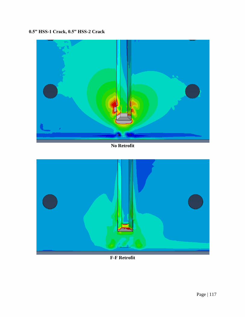
Page | 117

0.5” HSS-1 Crack, 0.5” HSS-2 Crack

No Retrofit

F-F Retrofit

Page | 118

F-M Retrofit

F-S Retrofit

Page | 119

M-F Retrofit

M-M Retrofit

Page | 120

M-S Retrofit

S-F Retrofit

Page | 121

S-M Retrofit

S-S Retrofit

Page | 122


No Retrofit

F-F Retrofit

Page | 123

F-M Retrofit

F-S Retrofit

Page | 124

M-F Retrofit

M-M Retrofit

Page | 125

M-S Retrofit

S-F Retrofit

Page | 126

S-M Retrofit

S-S Retrofit

Page | 127


No Retrofit

F-F Retrofit

Page | 128

F-M Retrofit

F-S Retrofit

Page | 129

M-F Retrofit

M-M Retrofit

Page | 130

M-S Retrofit

S-F Retrofit

Page | 131

S-M Retrofit

S-S Retrofit

Page | 132


No Retrofit

F-F Retrofit

Page | 133

F-M Retrofit

F-S Retrofit

Page | 134

M-F Retrofit

M-M Retrofit

Page | 135

M-S Retrofit

S-F Retrofit

Page | 136

S-M Retrofit

S-S Retrofit

Page | 137

XFEM Crack Modeling Comparison

The XFEM cracks in the parametric study from Part I were modeled along the interface

between the welds and the web. The XFEM cracks in Part II were modeled as being offset

slightly from the weld-web interfaces so that the cracks progresses through the interior of an

element rather than at the element’s edge. Screen shots of the two separate 2.7-m (9-ft) girder

subassembly models from Part I and Part II respectively illustrate the difference in the simulation

results. Figure 1 shows a screen shot of an un-retrofitted model from the parametric study in Part

I with a 51-mm (2.0-in.) HSS-1 crack and a 51-mm (2.0-in.) HSS-2 crack. Figure 2 shows a

screen shot of a model from Part II based on observed experimental crack growth with HSS-1

crack legs of 46-mm (1.8-in.) and 51-mm (2.0-in.) and an HSS-2 crack of 51-mm (2.0-in.). The

crack geometry in the model from Part II was most similar to the crack geometry in the model

from Part I.

Figure 1: Maximum principal stress contours of 2.7-m (9-ft) subassembly with XFEM cracks modeled along

the weld-web interfaces

Page | 138

Figure 2: Maximum principal stress contours of 2.7-m (9-ft) subassembly with XFEM cracks modeled offset

with the weld-web interfaces

As shown in Figure 1, with the cracks modeled along the weld-web interfaces, the highest

maximum principal stresses occurred at the connection plate-to-web weld toe and in the web-gap

between the connection plate and the flange. In Figure 2, with the cracks modeled as offset from

the weld-web interfaces, the highest maximum principal stresses occurred near the crack-tips.

The maximum principal stresses at the connection plate-to-web weld and in the web-gap were

significantly less than the maximum principal stresses in the first model. These results from the

second model are more consistent with experimental observations. Therefore, it is recommended

that the models from the parametric study in Part I be rerun with the XFEM cracks modeled as

offset from the interface between the welds and the web.

Documents

APPLICATIONS OF THE EXTENDED FINITE ELEMENT METHOD (XFEM …