Embed Size (px)
Citation preview

LINEAR ALGEBRA AND ITS
APPLICATIONS
EISBVIF?R Linear Algebra and its Applications 284 (1998) 1933228
Applications of second-Order cone programming ’
Miguel Soma Lobo a32, Lieven Vandenberghe b,*, Stephen Boyd c73, Herve Lebret dT4
a Information Systems Laboratory. Electrical Engineering Department, Stanford University, USA b Electrical Engineering Department, University of California. Los Angeles. USA
’ Information Systems Laboratory, Electrical Engineering Department, Stanford University. USA ’ Ecole Nationale Supkrieure de Techniques Avankes, Paris, France
Received 25 April 1997; accepted 26 January 1998
Submitted by D.P. O’Leary
Abstract
In a second-Order cone program (SOCP) a linear function is minimized over the inter- section of an affine set and the product of second-Order (quadratic) cones. SOCPs are nonlinear convex Problems that include linear and (convex) quadratic programs as spe- cial cases, but are less general than semidefinite programs (SDPs). Several efficient pri- maldual interior-Point methods for SOCP have been developed in the last few years. After reviewing the basic theory of SOCPs, we describe general families of Problems that tan be recast as SOCPs. These include robust linear programming and robust least- squares Problems, Problems involving sums or maxima of norms, or with convex hyper- bolic constraints. We discuss a variety of engineering applications, such as filter design, antenna array weight design, truss design, and grasping forte optimization in robotics. We describe an efficient primaldual interior-Point method for solving SOCPs, which shares many of the features of primaldual interior-Point methods for linear program-
* Corresponding author. E-mail: [email protected]. ’ Research supported in part by the Portuguese Govemment (under Praxis XXI), AFOSR
(under F49620-95-I-0318), NSF (under ECS-9222391 and EEC-9420565), and MURI (under F49620-95-1-0525). Associated Software is available at URL http://www-isl.stanford.edu/people/ boyd and from anonymous FTP to isl.stanford.edu in pub/boyd/socp.
’ E-mail: [email protected]. 3 E-mail: [email protected]. 4 E-mail: [email protected].
0024-3795/98/$19.00 0 1998 Elsevier Science Inc. All rights reserved. PlI:SOO24-3795(98)10032-0

194 M.S. Lobo et al. / Linear Algebra and its Applications 284 (1998) 193-228
ming (LP): Worst-case theoretical analysis Shows that the number of iterations required to solve a Problem grows at most as the Square root of the Problem size, while numerical experiments indicate that the typical number of iterations ranges between 5 and 50, al- most independent of the Problem size. 0 1998 Elsevier Science Inc. All rights reserved.
Keywords: Convex optimization; Quadratic programming; Semidefinite programming; Interior- Point methods
1. Introduction
1.1. Second-Order cone programming
We consider the second-Order cone program (SOCP)
minimize f Tx
subjectto IIAi~+b;ll<cTx+di, i= l,..., N, (1)
where x E R” is the optimization variable, and the Problem Parameters are f E R”, Ai E R(“‘_‘IX”, bi E (Wnl-‘, ci E R”, and di E R. The norm appearing in the constraints is the Standard Euclidean norm, i.e., IIuII = (uTu)‘12. We cal1 the constraint
I(AiX + bi 11 < CTX + di (2)
a second-Order cone constraint of dimension n;, for the following reason. The Standard or unit second-Order (convex) cone of dimension k is defined as
(which is also called the quadratic, ice-cream, or Lorentz cone). For k = 1 we define the unit second-Order cone as
%?,={tItER,O<t}.
The set of Points satisfying a second-Order cone constraint is the inverse image of the unit second-Order cone under an affine mapping:
IIAjx + bjll < c;x + d, w
and hence is convex. Thus, the SOCP (1) is a convex programming Problem since the objective is a convex function and the constraints define a convex set.
Second-Order cone constraints tan be used to represent several common convex constraints. For example, when nj = 1 for i = 1,. . . , N, the SOCP re- duces to the linear program (LP)

M.S. Lobo et al. I Linear Algebra and its Applications 284 (1998) 193-228
minimize f T~
subjectto O<cTx+di, i= l,..., N.
195
Another interesting special case arises when ci = 0, so the ith second-Order cone constraint reduces to ]]Aix + bi]] < di, which is equivalent (assuming di > 0) to the (convex) quadratic constraint ]]Aix + bi]]* < df. Thus, when all ci vanish, the SOCP reduces to a quadratically constrained linear program (QCLP). We will soon see that (convex) quadratic programs (QPs), quadratic- ally constrained quadratic programs (QCQPs), and many other nonlinear con- vex optimization Problems tan be reformulated as SOCPs as well.
1.2. Outline of the Paper
The main goal of the Paper is to present an overview of examples and appli- cations of second-Order cone programming. We Start in Section 2 by describing several general convex optimization Problems that tan be cast as SOCPs. These Problems include QP, QCQP, Problems involving sums and maxima of norms, and hyperbolic constraints. We also describe two applications of SOCP to ro- bust convex programming: robust LP and robust least squares. In Section 3 we describe a variety of engineering applications, including examples in filier de- sign, antenna array design, truss design, and grasping forte optimization. We also describe an application in Portfolio optimization.
In Section 4 we introduce the dual Problem, and describe a primal-dual po- tential reduction method which is simple, robust, and efficient. The method we describe is certainly not the only possible choice: most of the interior-Point methods that have been developed for linear (or semidefinite) programming tan be generalized (or specialized) to handle SOCPs as well. The concepts un- derlying other primal-dual interior-Point methods for SOCP, however, are very similar to the ideas behind the method presented here. An implementation of the algorithm (in C, with calls to LAPACK) is available via WWW or FTP [311*
1.3. Previous work
The main reference on interior-Point methods for SOCP is the book by Nesterov and Nemirovsky [32]. The method we describe is the primaldual al- gorithm of [32], Section 4.5, specialized to SOCP.
Adler and Alizadeh [l], Nemirovsky and Scheinberg [33], Tsuchiya [41] and Alizadeh and Schmieta [7] also discuss extensions of interior-Point LP methods to SOCP. SOCP also fits the framework of optimization over self-scaled cones, for which Nesterov and Todd [34] have developed and analyzed a special class of primal-dual interior-Point methods.

196 M.S. Lobo et al. I Linear Algebra and its Applications 284 (1998) 193-228
Other researchers have worked on interior-Point methods for special cases of SOCP. One example is convex quadratic programming; see, for example, Den Hertog [24], Vanderbei [42], and Andersen and Andersen [2]. As another example, Andersen has developed an interior-Point method for minimizing a sum of norms (which is a special case of SOCP; see Section 2.2) and de- scribes extensive numerical tests in [6]. This Problem is also studied by Xue and Ye [49] and Chan et al. [ZO]. Finally, Goldfarb et al. [27] describe an in- terior-Point method for convex quadratically constrained quadratic program- ming.
1.4. Relation to linear and semide$nite programming
We conclude this introduction with some general comments on the place of SOCP in convex optimization relative to other Problem classes. SOCP includes several important Standard classes of convex optimization Problems, such as LP, QP and QCQP. On the other hand, it is itself less general than semidefinite programming (SDP), i.e., the Problem of minimizing a linear function over the intersection of an affine set and the cone of positive semidefinite matrices (See, e.g., [43]). This tan be seen as follows: The second-Order cone tan be embedded in the cone of positive semidefinite matrices since
i.e., a second-Order cone constraint is equivalent to a linear matrix inequality. (Here k denotes matrix inequality, i.e., for X = XT ,Y = YT E iR”““, X 2 Y means zTXz > zTYz for all z E R”). Using this property the SOCP (1) tan be ex- pressed as an SDP
minimize fTx
subject to [
(cTx + di)l Aix + bi ~ o i = 1 . N 1 (3)
(AiX + bi)T CTX + di - ’ ” ” ’
Solving SOCPs via SDP is not a good idea, however. Interior-Point methods that solve the SOCP directly have a much better worst-case complexity than an SDP method applied to Problem (3): the number of iterations to decrease the duality gap to a constant fraction of itself is bounded above by O(n) for the SOCP algorithm, and by O(m) for the SDP algorithm (see [32]). More importantly in practice, each iteration is much faster: the amount of work per iteration is O(n2 Ei ni) in the SOCP algorithm and O(n2 Ei nf) for the SDP. The differente between these numbers is significant if the dimensions ni of the second-Order constraints are large. A separate study of (and code for) SOCP is therefore warranted.

M.S. Lobo et al. / Linear Algebra and its Applications 284 (1998) 193-228
2. Problems that tan be cast as SOCPs
197
In this section we describe some general classes of Problems that tan be for- mulated as SOCPs.
2.1. Quadratically constrained quadratic programming
We have already seen that an LP is readily expressed as an SOCP with one- dimensional cones (i.e., ni = 1). Let us now consider the general conuex qua- dratically constrained quadratic program (QCQP)
minimize xTPfl + 2qix + r.
subject to XTPix + 2qTx + ri < 0, i = 1. . .p, (4)
where Po, P,, . . . , Pp E IR”“” are symmetric and positive semidefinite. We will assume for simplicity that the matrices fl are positive definite, although the Problem tan be reduced to an SOCP in general. This allows us to write the QCQP (4) as
2
minimize II
Pi’2x + Pi”2q0 II
+ ro - q~P;‘qo
subject to II fl’12x + e-‘j2 qi
II ‘+rj-q~P,-lqiQO, i= l,...,p >
which tan be solved via the SOCP with p + 1 constraints of dimension n + 1
minimize t
subject to IIPi”x + P;“2qojl 6 t, (5)
llpi”2x + ~~“2qi(l < (qT4-‘qi - rj)li2, i = 1,. . . ,p,
where t E R’ is a new optimization variable. The optimal values of Problems (4) and (5) are equal up to a constant and a Square root. More precisely, the optimal value of the QCQP (4) is equal to p*’ + ro - q~Pö’qo, where p* is the optimal value of the SOCP (5).
As a special case, we tan solve a convex quadratic programming Problem (Qp)
minimize xTPox + 2qox + r. subject to aTx 6 bi, i = 1, . ..lP
(PO + 0) as an SOCP with one constraint of dimension n + 1 and p constraints of dimension one
minimize t
subject to llPi’2x + Pi1’2qo(I < t, a:x 6 bi, i = 1, . ,p,
where the variables are x and t.

198 MS. Lobo et at’. I Linear Algebra and its Applications 284 (1998) 193-228
2.2. Problems involving sums and maxima of norms
Problems involving sums of norms are readily cast as SOCPs. Let F; E R”‘“” and gi E lV, i = 1,. . . ,p, be given. The unconstrained Problem
minimize ~llF;x+gill
i=l
tan be expressed as an SOCP by introducing auxiliary variables tl , . . . , tp
minimize eti i=l
subject to IIF+ + gill < tj, j = 1,. . . ,p.
The variables in this Problem are x E R” and ti E R. We tan easily incorporate other second-Order cone constraints in the Problem, e.g., linear inequalities on x.
The Problem of minimizing a sum of norms arises in heuristics for the Steiner tree Problem [25,49], optimal location Problems [37], and in total-variation im- age restoration 20. Specialized methods are discussed in [6,4,23,25,20].
Similarly, Problems involving a maximum of norms tan be expressed as SOCPs: the Problem
minimize iyap 11 Ex + gi 11 < >
is equivalent to the SOCP
minimize t
subjectto Ilfix+giIj<t, i= l,...,p
in the variables x E DY’ and t E R. As an interesting special case of the sum-of-norms Problem, consider the
complex !i -norm approximation Problem minimize Ikr - Hl,
where x E Cq, A E Cpxq, b E V, and the er-norm on CP is defined by IIv]Ir = CCr IVil. This Problem tan be expressed as an SOCP withp constraints of dimension three
minimize Cti
i=l
in the variables z = [%?x’ 3xT]’ E R*q, and tie In a similar way the complex & norm approximation Problem tan be formulated as a maximum-of-norms Problem.
M.S. Lobo et al. l Linear Algebra and its Applications 284 (1998) 193-228 199
As an extension that includes as special cases both the maximum and sum of norms, consider the Problem of minimizing the sum of the k largest norms IIE;lx + gil), i.e., the Problem
minimize @il (6) subject to IIfix+g;]l =yi, i = l,... ,p,
where Y[II, 421, . . . , hl are the numbers yl ,y2, . . . y, sorted in decreasing Order. It tan be shown that the objective function in Problem (6) is convex and that the Problem is equivalent to the SOCP
minimize kt + eyi i=l
subjectto j(f$x+gil(<t+yi, i= l,..., p, YibO, i= l,..., p,
where the variables are x, y E Rp, and t. (See, e.g. [44] or [17] for further discus- sion.)
2.3. Problems with hyperbolic constraints
Another large class of convex Problems tan be cast as SOCPs using the fol- lowing fact:
w2 <XY, 2w
x a 0, y30 * IK Ill <x+y, X-Y
and, more generally, when w is a vector,
wTw 6 xy, 2w
x 2 0, y>o * IK Ill <x+y. X-Y
We refer to these constraints as hyperbolic constraints, since they describe half a hyperboloid.
As a first application, consider the Problem
minimize f: 1 /(aT_x + bi) i=l
subjectto aTx+bi>O, i= 1,. . . ,P, cTx+d;~O, i= 1,“‘) q,
which is convex since l/(uTx + bi) is convex for a:x + bi > 0. This is the prob- lem of maximizing the harmonic mean of some (positive) affine functions of x, over a polytope. This Problem tan be cast as an SOCP as follows. We first in- troduce new variables ti and write the Problem as one with hyperbolic con- straints:
200 M.S. Lobo et al. I Linear Algebra and its Applications 284 (1998) 193-228
minimize i=l
subjectto ti(aTx+bi) > 1, ti>O, i= l,..., p,
CTX+di>Oj i= l,..., 4.
By Eq. (7) this tan be cast as an SOCP in x and t
P
minimize c 6 i=l
subject to /1[LZTX+Ii-ti]]]
<aT.X+bi+ti, i= l,...,p
CTX+di 20, i= l,..., 4.
As an extension, the quadratic/linear fractional Problem
minimize ’ IIfiX + gil12 c ;=r a?X + bi
subjectto aTx+b;>O, i= l,..., p,
where 4 E Rsxn, gi E RqZ, tan be cast as an SOCP by first expressing it as
P
minimize c ti
i=l
subject to (EX + gi)T(fix + gi) f ti(aTx + bi), i = 1, . . . ,p,
aTX+bi>O, i=l,..., p,
and then applying Eq. (8). As another example, consider the logarithmic Chebyshev approximation
Problem
minimize max 11% (4x) - 1% (bi) 1, (9
where A = [ur . . . uplT E Rp”“, b E Rp. We assume b > 0, and interpret log(uTx) as -oc when uTx < 0. The purpose of Problem (9) is to approximately solve an overdetermined set of equations Ax KZ b, measuring the error by the maximum logarithmic deviation between the numbers uTx and bi. To cast this Problem as an SOCP, first note that
Ilog(uTx) - log(bi)I = log max(uTx/bj, bi/uTn)
(assuming uTx > 0). The log-Chebyshev Problem (9) is therefore equivalent to minimizing maxi max(u’x/bl, bi/uTx), or:
This
M.S. Lobo et al. i Linear Algebra and its Applications 284 (1998) 193-228
minimize t
subject to l/t < aTx/bi < t, i = 1,. . . ,p.
tan be expressed as the SOCP
minimize t
subject to ayx/bi 6 t, i = 1,. . ,p,
201
II[t-a;x/hII/ <t+aTx/bi, i= 1,. . . ,P.
As a final illustration of the use of hyperbolic constraints, we consider the Problem of maximizing the geometric mean (or just product) of nonnegative affine functions (from Nesterov and Nemirovsky [32], p. 227):
P
maximize n( a:x + bi) “’ i=l
subjectto aTx+bibO, i= 1,. . . ,P.
For simplicity, we consider the special case p = 4; the extension to other values of p is straightforward. We first reformulate the Problem by introducing new variables tl, t2, and t3, and by adding hyperbolic constraints:
maximize t3
subject to (aTx + bz)(aTx + b2) 2 tf, aTx + bz 2 0, a:x + b2 2 0,
(a;x + bj)(aTx + bd) 2 $, aTx + b3 2 0, aix + bd > 0,
tlt2 > t:, tl 2 0, t2 2 0.
Applying Eq. (7) yields an SOCP.
2.4. Matrix-fractional Problems
The next class of Problems are matrix-fractional optimization Problems of the form
minimize (fi + g)‘(& + x& + . . . + x/~)-‘(FX + g) subject to Po + x& + . . . + xpPp + 0, x B 0, (10)
where fl = P,? E IR”““, F E iRnxp and g E R”, and the Problem variable is x E Rp. (Here + denotes stritt matrix inequality and > componentwise vector inequality.)
We first note that it is possible to solve this Problem as an SDP minimize t
P(x) fi+g F.
1 (Fx +g)T t - 7

202 M.S. Lobo et al. I Linear Algebra and its Applications 284 (1998) 193-228
where P(x) = Po + xiPI + . . . + xpPp. The equivalence is readily demonstrated by using Schur complements, and holds even when the matrices fl are indef- inite. In the special case where the Pi are positive semidefinite, we tan refor- mulate the matrix-fractional optimization Problem more efficiently as an SOCP, as shown by Nesterov and Nemirovsky [32]. We assume for simplicity that the matrix PO is nonsingular (see [32] for the general derivation).
We Claim that Problem (10) is equivalent to the following optimization prob- lem in tO,tl,. ..,tn E R, YO, Yi, . . . . yp E R”, andx:
minimize t. + tl + . . + tp
subject to Pi’2yo + P:‘2y, + . . + Pj/2yp = FX + g,
llYol12 G to,
llJ+112<tiXi, iz l,...,p,
ti,X, 2 0, i= l,...,p,
which tan be cast as an SOCP using Eq. (8)
(11)
minimize t. + t, + . . + tp
subject to Pi’2yo + 2 p,“‘y, = Fx + g, i=l
2Yo Ib Ill to - 1
<to+l,
<ti+Xi, i= l,..., p.
The equivalence between Problems (10) and (11) tan be seen as follows. We first eliminate the variables ti and reduce Problem (11) to
minimize y,Ty0 + y;yi /xi + . . . + ypyp/xp
subject to Pii2yo + P:‘2y, + . + Pj”yp = Fx + g, x 3 0
(interpreting O/O = 0). Since the only constraint on Yi is the equality constraint, we tan optimize over Yi by introducing a Lagrange multiplier 1 E R” for the equality constraint, which gives us yi in terms of u and x:
2Yo = -Pi12A. and 2Y, = -xip1.‘12A, i = 1,. . . ,p.
Next we Substitute these expressions for yj and obtain a minimization Problem in A and x:
minimize 4AT(Po+x,P, +-+xppPp)A
subject to (Po + x,P, + . . . + xpPp)A = -2(Fx + g), x 2 0.
Finally, eliminating A. yields the matrix-fractional Problem (10).

M.S. Lobo et al. / Linear Algebra and its Applicatiom 284 (1998) 193-228
2.5. SOC-representable functions and sets
203
The above examples illustrate several techniques that tan be used to deter- mine whether a convex optimization Problem tan be cast as an SOCP. In this section we formalize these ideas with the concept of a second-Order cone repre- sentation of a set or function, introduced by Nesterov and Nemirovsky [32], Section 6.2.3.
We say a convex set C C R” is second-Order cone representable (abbreviated SOC-representable) if it tan be represented by a number of second-Order cone constraints, possibly after introducing auxiliary variables, i.e., there exist A_ E R(ni-l)X(n+m) I , bi E llF1, c, E lR”+m, d,, such that
XEC _ gJJE[w” S.t. llAi[z] +biil<cT[z] +di, i= l,...,N.
We say a function f is second-Order cone representable if its epigraph ((~74 If(x) Gt] h as a second-Order cone representation. The practical conse- quence is that iff and C are SOC-representable, then the convex optimization Problem
minimize f(x)
subject to x E C
tan be cast as an SOCP and efficiently solved via interior-Point methods. We have already encountered several examples of SOC-representable func-
tions and Sets. SOC-representable functions and sets tan also be combined in various ways to yield new SOC-representable functions and Sets. For example, if Cl an C, are SOC-representable, then it is straightforward to show that aCI (o! B 0), Cl fl CZ and Cl + CZ are SOC-representable. If fi and f2 are SOC-rep- resentable functions, then ufi (a 2 0), fl +fl, and max{fi,fi} are SOC-repre- sentable.
As a less obvious example, if fi , f2 are concave with fi (x) 2 0, f2(x) > 0, and -fl and -f2 are SOC-representable, thenf& is concave and -f& is SOC-rep- resentable. In other words the Problem of maximizing the product of f, and f2,
maximize fi (x)f2 (x)
subject to fi (x) 3 0, f*(x) 3 0
tan be cast as an SOCP by first expressing it as
maximize t subject to tl t2 B t,
fl(X) 2 t1, h?(x) 3 t2r
t1 3 0, t2 2 0
and then using the SOC-representation of -fl and -f2.

204 M.S. Lobo et al. / Linear Algebra and its Applications 284 (1998) 193-228
SOC-representable functions are closed under composition. Suppose the convex functions fr and f2 are SOC-representable and fr is monotone nonde- creasing, so the composition g given by g(x) = fr ($(x)) is also convex. Then g is SOC-representable. To see this, note that the epigraph of g tan be expressed as
{(x, 4 I g(x) < t) = {(x, 4 I 3 E R s.t. fl(s) < 4h(X) <s>
and the conditions fr(s) < t, f*(x) < s tan both be represented via second-Order cone constraints.
2.6. Robust linear programming
In this section and the next we show how SOCP tan be used to solve some simple robust convex optimization Problems, in which uncertainty in the data is explicitly accounted for.
We consider a linear program
minimize cTx
subject to ayx< bi, i = 1,. . . ,m,
in which there is some uncertainty or Variation in the Parameters c, ai, bi. To simplify the exposition we will assume that c and bi are fixed, and that the ai are known to lie in given ellipsoids
ai E 8; = (2% +&4 1 1(uII < l},
where Pi = P,? 2 0. (If Pi is Singular we obtain ‘flat’ ellipsoids, of dimension rank (fl).)
In a worst-case framework, we require that the constraints be satisfied for all possible values of the Parameters ai, which leads us to the robust linear program
minimize cTx
subjectto aTx<bi, forallaiEB,, i= l,...,m. (12)
The robust linear constraint aTx < bi for all ai E 8; tan be expressed as
max{aTx (at E &;} =qTx+ Ijfixll< bi,
which is evidently a second-Order cone constraint. Hence the robust LP (12) tan be expressed as the SOCP
minimize cTx
subject to aTx + j\P;xll< bi, i = 1,. . . , m.
Note that the additional norm terms act as ‘regularization terms’, discauraging large x in directions with considerable uncertainty in the Parameters ai. Note that conversely, we tan interpret a general SOCP with bi = 0 as a robust LP.

M.S. Lobo et al. / Linear Algebra and its Applications 284 (1998) 193-228 205
The robust LP tan also be considered in a statistical framework [47], Section 8.4. Here we suppose that the Parameters ai are independent Gaussian random vectors, with mean üi and covariance Zi. We require that each constraint a:x < bi should hold with a probability (confidence) exceeding q, where v] 2 0.5, i.e.,
Prob(a’x < bi) 3 u. (13)
We will Show that this probability constraint tan be expressed as an SOC con- straint.
Letting u = aTx, with o denoting its variance, this constraint tan be written as
Prob
Since (U - U)/J o is a zero mean unit variance Gaussian variable, the probabil- ity above is simply @((bi - u)/&?), where
Q(z) = & _i emt212dt s
is the CDF of a zero mean unit variance Gaussian random variable. Thus the probability constraint (13) tan be expressed as
or, equivalently,
u + @‘(q),,% < b;.
From u = ü:x and CJ = xTCix we obtain
ÜTX + @-‘(~)llCf’2Xll <bi.
Now, provided u] b 1/2 (i.e., G-‘(q) > 0), this constraint is a second-Order cone constraint.
In summary, the Problem
minimize cTx
subject to Prob (a:x < b,) > q, i = 1, . . . , m
tan be expressed as the SOCP
minimize cTx
subject to ~fx + Qi-1(r])llZ~‘2xll <bi, i = 1,. . , m.
We refer to Ben-Tal and Nemirovsky [16], and Oustry, El Ghaoui, and Leb- ret [35] for further discussion of robustness in convex optimization. For control applications of robust LP, see Boyd, et al. [lO].

206 MS. Lobo et al. / Linear Algebra and its Applications 284 (1998) 193-228
2.7. Robust least-squares
Suppose we are given an overdetermined set of equations Ax x b, where A E W”“” , b E [w” are subject to unknown but bounded errors 6A and 6b with IlVl fp, 116bll 6 5 ( w h ere the matrix norm is the spectral norm, or maximum Singular value). We define the robust least-squares solution as the Solution X E R” that minimizes the largest possible residual, i.e., i is the Solution of
minimize I,sA,, m$,,, ~ 5 II (‘4 + hA)x - (b + hb) 11. (14)
This is the robust least-squares Problem introduced by El Ghaoui and Lebret [26] and by Chandrasekaran et al. [18,19] and Sayed et al. [39]. The objective function in Problem (14) tan be written in a closed form, by noting that
,,&,,,npai~~,,,~ ll(A + dA)x - (b + 6b)II = max max yT(Ax - b) + yTGAx - yTGb
IIW <P> II~~II G 5 IIYII a 1
= max maxyT(Ax - b) +zTx+ 5 11~11 c P IIYII a 1
= 11-4~ - bll + PIIxII + 5. Problem (14) is therefore equivalent to minimizing a sum of Euclidean norms
minimize IIAx - blJ + pIIxII + 5.
Although this Problem tan be solved as an SOCP, there is a simpler Solution via the Singular value decomposition of A. The SOCP-formulation becomes useful as soon as we put additional constraints on x, e.g., nonnegativity constraints.
A Variation on this Problem is to assume that the rows ai of A are subject to independent errors, but known to lie in a given ellipsoid: ai E bi, where
&i = {Zi +fiU ( (IU(I 6 1) (fl = Pi’ F 0).
We obtain the robust least squares estimate x by minimizing the worst-case re- sidual
minimize Tf; ( $ (aTx - biJ2) “‘.
We first work out the objective function in a closed form
$T; IÜ;x - b, + uTPixj . IZ f$y max { ZTX - bi + uTflx, -gTx + bi - uTex}
.
= max {ÜTx - bi + IIfi~ll, -$x + bi + Ilfi~ll}
= IZTX- bi/ + Ilfi~ll.
05)

MS. Lobo et al. I Linear Algebra and its Applicatiom 284 (1998) 193-228
Hence, the robust least-squares Problem (15) tan be formulated as
207
minimize (
2 ( IKTx - bi1 + IIP;ni[)” “2, kl )
which tan be cast as the SOCP
minimize s
subject to Iltll <s
I~TX-bjl+Il&XIJ<ti, i= l,.. n .> .
These two robust variations on the least-squares Problem tan be extended to allow for uncertainty on b. For the first Problem, suppose the errors 6A and 6b are bounded as II[&t 6b] (1 6 p, Using the same analysis as above it tan be shown that
,,lsjrd~~ipIl(~+~~)x- (b+bb)lI = Ib-bll sp ; ll[ Ill .
The robust least-squares Solution tan therefore be found by solving
minimize IIAx - bll + p T IR Ill
In the second Problem, we tan assume bi is bounded by bi E [b; - pi, bi + Pi]. A straightforward calculation yields
minimize 2 (IZTX - ZiJ + ((qXJ[ +pi)2 i=l
which tan be easily cast as an SOCP.
3. Applications
3.1. Antenna array weight design
In an antenna array the Outputs of several antenna elements are linearly combined to produce a composite array output. The array output has a direc- tional Pattern that depends on the relative weights or scale factors used in the combining process, and the goal of weight design is to choose the weights to achieve a desired directional Pattern.
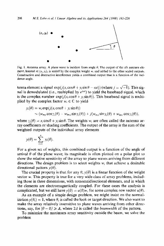
We will consider the simplest model, an array of omnidirectional antenna elements in a plane, at positions (xi, yi), i = 1, . . . , n (see Fig. 1). A unit plane wave, of frequency o, is incident from angle 0. We assume the wave number is one, i.e., the wavelength is A. = 27~ This incident wave induces in the ith an-
208 M.S. Lobo et al. l Linear Algebra and its Applications 284 (1998) 193-228
(Xt,Yi) ??0
0 ?? 4 _-.__P
0 0
Fig. 1. Antenna array. A plane wave is incident from angle H. The output of the ith antenna ele- ment, located at (x,,J+), is scaled by the complex weight W, and added to the other scaled Outputs. Constructive and destructive interference yields a combined output that is a function of the inci- dence angle.
tenna element a Signal exp(j(xi COS 0 + yi sin t9 - ot)) (where j = fl). This sig- na1 is demodulated (i.e., multiplied by ~9~) to yield the baseband Signal, which is the complex number exp(j(q cos 0 + yL sin 13)). This baseband Signal is multi- plied by the complex factor wi E C to yield
yi( 0) = Wi eXpG(Xj COS tJ + JJf sin 0))
= (%z,~~~~Y~(@ - Wm,isiny,(S)) +j(w~e,isinYi(@ + Wim.iCOSYj(~)),
where y,(O) = XicosfI +yisin8. The weights wi are often called the antenna ar- ray coefficients or shading coefficients. The output of the array is the sum of the weighted Outputs of the individual array elements
Y(@ = 2 Yd@. i=i For a given set of weights, this combined output is a function of the angle of arrival 8 of the plane wave; its magnitude is often plotted on a polar plot to show the relative sensitivity of the array to plane waves arriving from different directions. The design Problem is to select weights Wi that achieve a desirable directional Pattern y( 0).
The crucial property is that for any 0, y(B) is a linear function of the weight vector w. This property is true for a very wide class of array Problems, includ- ing those in three dimensions, with nonomnidirectional elements, and in which the elements are electromagnetically coupled. For these cases the analysis is complicated, but we still have y(O) = a(O)w, for some complex row vector a(O).
As an example of a simple design Problem, we might insist on the normal- ization y( 0,) = 1, where 0, is called the look or target direction. We also want to make the array relatively insensitive to plane waves arriving from other direc- tions, say, for (0 - 8,( 2 A, where 24 is called the beamwidth of the Pattern.
To minimize the maximum array sensitivity outside the beam, we solve the Problem
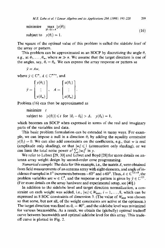
M.S. Lobo et al. l Linear Algebra and its Applications 284 (1998) 193-228 209
minimize ,,m,rttd Iy( 0) (
subject to ~(0,) = 1. (16)
The Square of the optimal value of this Problem is called the sidelobe leuel of the array or Pattern.
This Problem tan be approximated as an SOCP by discretizing the angle 19, e.g., at 0,) . . . , O,, where m » n. We assume that the target direction is one of the angles, say, 0, = &. We tan express the array response or Pattern as
Y=Aw,
where jj E C”, A E Cmxn, and
Problem (16) tan then be approximated as
minimize 1
subject to Iy(&)( <t for (& - kJ1 > A, y(&) = 1,
which becomes an SOCP when expressed in terms of the real and imaginary Parts of the variables and data.
This basic Problem formulation tan be extended in many ways. For exam- ple, we tan impose a null in a direction Br by adding the equality constraint y(0,) = 0. We tan also add constraints on the coefficients, e.g., that w is real (amplitude only shading), or that ]wi] 6 1 (attenuation only shading), or we tan limit the total noise power o* Ei lwil* in y.
We refer to Lebret [29, 301 and Lebret and Boyd [28] for more details on an- tenna array weight design by second-Order cone programming.
Numericalexample: The data for this example, i.e., the matrix A, were obtained from field measurements of an antenna array with eight elements, and angle of in- cidence 8 sampled in 1 o increments between -60’ and +60°. Thus, A E C12’ ‘*, the problem variables are w E C8, and the response or Pattern is given by j E C12’. (For more details on the array hardware and experimental setup, see [40].)
In addition to the sidelobe level and target direction normalization, a con- straint on each weight was added, i.e., Iwi( < W,,,, i = 1, . . . ,8, which tan be expressed as 8 SOC constraints of dimension 3. (The value of W,,, was Chosen so that some, but not all, of the weight constraints are active at the Optimum.) The target direction was fixed as 8, = 40°, and the sidelobe level was minimized for various beamwidths. As a result, we obtain the (globally) optimal tradeoff curve between beamwidth and optimal sidelobe level for this array. This trade- off curve is plotted in Fig. 2.

210 M.S. Lobo et al. l Linear Algebra and its Applications 284 (1998) 193-228
Half beamwidth A
Fig. 2. Optimal tradeoff curve of sidelobe level versus half-beamwidth d
3.2. Grasping forte optimization
We consider a rigid body held by N robot fingers. To simplify formtdas we assume the Center of mass of the body is at the origin. The fingers exert contact forces at given Points p' , . . . ,p” E R3. The inward pointing normal to the sur- face at the ith contact Point is given by the (unit) vector U’ E R3, and the forte applied at that Point by F’ E R’.
Esch contact forte F’ tan be decomposed into two Parts: a component (v’)~F’v’ normal to the surface, and a component (1 - $(u’)~)F’, which is tan- gential to the surface. We assume the tangential component is due to static fric- tion and that its magnitude cannot exceed the normal component times the friction coefficient p > 0, i.e.,
Il(I - ui(ui)')FiII < ,u(~)~F’, i= l,...,N. (17)
These friction-cone constraints are second-Order cone constraints in the vari- ables F’.
Finally, we assume that external forces and torques act on the body. These are equivalent to a Single external forte Fext acting at the origin (which is the center of mass of the body), and an external torque Text. Static equilibrium of the body is characterized by the six linear equations
N
c F’ + Fe”’ = 0, 2 pi x F’ + Text = 0. (18) i=l i=l
The stable grasp analysis Problem is to find contact forces F’ that satisfy the friction cone constraints (17), the static equilibrium constraints (18), and cer- tain limits on the contact forces, e.g., an upper bound (II~)~& < fmax on the nor-
M.S. Lobo et al. / Linear Algebra and its Applications 284 (1998) 193-228 211
mal component. When the limits on the contact forces are SOC-representable, this Problem is a second-Order cone feasibility Problem.
When the Problem is feasible we tan select a particular set of forces by op- timizing some criterion. For example, we tan compute the gentlest grasp, i.e., the set of forces F’ that achieves a stable grasp and minimizes the maximum normal forte at the contact Points, by solving the SOCP
minimize t
subject to (u’)Tfi<t, i = l,..., N, (17), (18).
For more details on grasping forte optimization we refer to [22,12,1 l] and the references in those Papers. In [22] the friction cone constraints is approx- imated by a set of linear inequalities, so grasping forte optimization Problems reduce to LPs. More recently Buss et al. [12,1 l] have used SDP embedding of the second-Order cone constraints as discussed at the end of Section 1.2. (Note that in this Problem the second-Order cone constraints have dimension 3, so the drawbacks that the SDP embedding has in general, are almost in- significant.)
3.3. FIR jilter design
We denote by hO, hl,. . . , h,_l E [w the coefficients (impulse response) of a fi- nite impulse response (FIR) filter of length n. This means the filter output se- quence or Signal y : Z -f R is related to the input u : h + R via convolution
n-l
y(k) = C hiu(k - i). 1=0
The frequency response of the filter is the function H: [0,2n] + C defined as
n-l
H(o) = c hke-jko, k=O
where j = J-1 and o is the (discrete-time) frequency variable. Minimax complex transfer function design: We first consider the Problem of
designing a filter that approximates a desired frequency response as well as pos- sible. We assume the desired frequency response is specified by the complex numbersH?,i= l,... ,N, that are the desired values of the transfer function at the frequencies Oi, i = 1, . . . , N. The design Problem is to choose filter coef- ficients that minimize the maximum absolute deviation
minimize i~ax, 1 H( Oi) - Hy 1 1 >
over all possible COeffiCientS hk. This is a complex C,-approximation Problem,
212 h4.S. Lobo et al. / Linear Algebra and its Applications 284 (1998) 193-228
- 1 e-jw e-j2w . . . e-i(n-lh
1 e-iw e-i2w . . e-i(~-l)~z minimize . . . . .
!
>
1 e-h e-%Jv . . . e-j(n-lhv
which tan be cast as an SOCP using the results of Section 2.2. Minimax linearphase lowpassfilter design: As a second filter design example, we
consider the special case where the filter coefficients are symmetric: hk = hn-k-l. For simplicity we assume n is even. The frequency response simplifies to
n/2-1
H(o) = c hk(e-iko + e-i(n-kPl)o) k=O
42-1
= 2e-‘“(“p’)‘2 c hkCOS((k - (TI - 1)/2)0). k=O
This is called a linear phasefilter because the transfer function tan be factored into a pure delay (which has linear Phase), e-iw(n-‘)/2, and a real-valued term,
n/2- 1
T(o) = 2 c h kcos((k-(n- 1)/40), (19) k=O
which is a trigonometric polynomial with coefficients hi. Note that IH(o)I = IT(w)I.
It was observed already in the 1960s that many interesting design Problems for linear Phase FIR filters tan be cast as LPs. We illustrate this with a simple example involving low-pass filter design, with the following specifications. In the stopband, o, < o < rc, we impose a minimum attenuation: IH(o)I < LX In the passband, 0 < o 6 op, we want the magnitude of the transfer function to be as close as possible to one, which we achieve by minimizing the maximum deviation IIH(o)l - 11. This leads to the following design Problem
minimize o<:ax-U IlH(o)l - 11 , (20) subject to IH(;)li 8, o, <o 6 n
where the variables are the coefficients hi, i = 0, . . . , n/2 - 1, and op < o, < n, and /? > 0, are Parameters.
In the form given, the design Problem (20) is not a convex optimization Problem, but it tan be simplified and recast as one. First we replace IH(w)I by IT(o)l, the trigonometric polynomial (19). Since we tan Change the sign of the coefficients h, (hence, T) without affecting the Problem, we tan assume without loss of generality that T(0) > 0. The optimal value of the Problem is always less than one (which is achieved by h, = 0), so in fact we tan assume that T(w) > 0 in the passband. This yields the following optimization Problem

M. S. Lobo et al. / Linear Algebra and its Applications 284 (1998) 193-228 213
minimize O<mOTxO IT(o) - 11 . (21)
subject to ]T(w)]P< /?, o, < w < rc.
This Problem is convex, but has infinitely many constraints. We tan form an ap- proximation by discretizing the frequency variable w: let Oi, i = 1, . . . , NI - 1, be Nr frequencies in the passband, and oi, i = NI, . . . , N - 1, be N - Nr frequencies in the stopband. The discretized Version of Eq. (21) is the LP
minimize t n/2-l
subjectto 1--~~2~hkcos((k-(~-1)/2)wi)~1+~, k=O
i= l,...,Nr - 1 n/2-1
(22)
b< Chk~0~((k-(n-l)/2)w;)~p, i=NI,...,N k=O
with as variables ha, . . ., hnf2-r. (See also the course notes [17].) Bounds on the deviation from specifications between Sample Points tan be
derived, showing that the Solution of the discretized Problem converges to the solution of the continuous Problem as the discretization interval becomes small. See, e.g., [21,45].
Minimax dB linear Phase lowpass$lter design: We now describe a Variation on the design Problem just considered, in which the magnitude deviation in the passband is measured on a logarithmic scale, which more accurately captures actual filter design specifications. This Problem cannot be formulated as an LP, but tan be cast as an SOCP.
We suppose the deviation of the transfer function magnitude from one, in the passband, is measured on a logarithmic scale, i.e., we use the objective
o<mm~xu IlogIH(w)I - log11 = opuyu IlogI~(~)lI. -. - P -. , P
This objective is, except for a constant factor, the minimax deviation of the fil- ter magnitude measured in decibels (dB) (which uses 20 log,, instead of log).
We tan handle the resulting Problem in a way similar to the minimax low- pass filter Problem described above. The logarithmic deviation of T is handled using SOCP in a way similar to the log-Chebyshev approximation Problem of Section 2.3: we introduce a new variable t, and modify Problem (22) as
minimize t n/2-I
subject to l/t<2 C hkCOS((k-(n- l)/Z)Wi)<t, i= l,...,Nr - 1, k=O
n/2-I
-fi<2~hkCOS((k-(n-1)/2)wi)<p, i=NI,...,N. k=O
(23)
214 M.S. Lobo et al. I Linear Algebra and its Applications 284 (1998) 193-228
Note that here, the objective t represents the fractional deviation of \H(w)] from one, whereas in Problem (22) t represents the absoZute deviation. The optimal value (in dB) of the minimax dB design Problem is given by 20 log,,+*, where t* is the optimal value of Problem (23).
After reformulating the hyperbolic constraints as second-Order constraints, we obtain the SOCP
minimize t
subject to 2 IN Ill Gu+t,
u-t n/2-1
u<2 C hkcos((k- (n- 1)/2)0,)<t, i= l,...,Ni - 1, k=O
n/2-1
-8<2 Chkcos((k-(n_1)/2)wi)gB, i=Nl,...,N.
k=O
(24)
For more on this subject, see [8], p. 380, [36], Section 5.6. The topic of FIR fil- ter design using convex optimization and interior-Point algorithms is pursued in much greater detail in [45,46, 381.
3.4. Portfolio optimization with loss risk constraints
We consider a classical Portfolio Problem with n assets or Stocks held over one period. We let xi denote the amount of asset i held at the beginning of (and throughout) the period, and pj will denote the price Change of asset i over the period, so the return is r = p’x. The optimization variable is the Portfolio vec- tor x E R”. The simplest assumptions are x, 2 0 (i.e., no short positions) and Xi + . . . +x, = 1 (i.e., unit total budget).
We take a simple stochastic model for price changes: p E R” is Gaussian, with known mean p and covariance C. Therefore with Portfolio x E [w”, the re- turn r is a (scalar) Gaussian random variable with mean 7 = P’X and variance or = xTZx. The choice of Portfolio x involves the (classical, Markowitz) trade- off between return mean and variance.
Using SOCP, we tan directly handle constraints that limit the risk of various levels of 10s~. Consider a loss risk constraint of the form
Prob(r < a) < 8, (25) where c( is a given unwanted retum level (e.g., an excessive 10s~) and fl is a given maximum probability. As in the stochastic interpretation of the robust LP of Section 2.6, we tan express this constraint using the CDF Q> of a unit Gaussian random variable. The inequality (25) is equivalent to
P’x + @-‘(p))lc”2xll > u. (26)

M.S. Lobo et al. i Linear Algebra and its Applications 284 (1998) 193-228 215
Provided ß 6 i (i.e., W’(ß) < 0), this loss risk constraint is a second-Order cone constraint. (If ß > i, the loss risk constraint becomes concave in x.)
The Problem of maximizing the expected return subject to a bound on the loss risk (with ß < i), tan therefore be cast as a simple SOCP with one sec- ond-Order cone constraint
maximize P’x
subject to p’x+ O-‘(ß))l&xll 2 ~1, x 2 0, 2~~ = 1. i=l
There are many extensions of this simple Problem. For example, we tan impose several loss risk constraints, i.e.,
Prob(r<ai)<ßi, i== l,..., k,
(where ßi < $, which expresses the risks (ßJ we are willing to accept for various levels of loss (IX,).
As another Variation, we tan handle uncertainty in the statistical model @, Z) for the price changes during the period. Suppose we have N different possi- ble seenarios, each of which is modeled by a simple Gaussian model for the price Change vector, with mean pk and covariance &. We tan then take a worst-case approach and maximize the minimum of the expected returns for the N different seenarios, subject to a constraint on the loss risk for each scenario. In other words, we solve the SOCP
maximize rn/r $J.x
subjectto ~~x+@-i(ß)~~Z:‘2xII 2~, k= l,...,N, ~20, eXi= 1. i=l
Note that the constraints impose the loss risk limit under all N seenarios. As another (Standard) extension, we tan allow short positions, i.e., x, < 0.
To do this we introduce variables xi,,,,s and Xsh,,rt, with
n
Xlong z 0, Xshort 2 0, x = -%ng - Xshortr c Xshort < q xlong~ i=l 1=1
(The last constraint limits the total short Position to some fraction 9 of the total long Position.)
3.5. Truss design
Ben-Tal and Bendsoe in [13] and Nemirovsky in [ 141 consider the following Problem from structural optimization. A structure of k linear elastic bars con- nects a set of p nodes. The task is to size the bars, i.e., determine Xi, the cross-
216 MS. Lobo et al. i Linear Algebra and its Applications 284 (1998) 193-228
sectional areas of the bars, that yield the stiffest truss subject to constraints such as a total weight limit.
In the simplest version of the Problem we consider one fixed set of externally applied nodal forces _& i = 1, . , p; more complicated Versions consider multi- ple loading seenarios. The vector of small node displacements resulting from the load forces f will be denoted d. One objective that measures stiffness of the truss is the elastic stored energy ifTd, which is small if the structure is stiff. The applied forces f and displacements d are linearly related: f = K(x)d, where
K(X) ’ 2XiKl i=l
is called the stiffness matrix of the structure. The matrices K, are all symmetric positive semidefinite and depend only on fixed Parameters (Young’s modulus, length of the bars, and geometry). To maximize the stiffness of the structure, we minimize the elastic energy, i.e., fTK(x)-‘f/2. Note that increasing any Xi will decrease this objective, i.e., stiffen the structure.
We impose a constraint on the total volume (or equivalently, weight), of the structure, i.e., Ei EJi 6 U,,,, where Zi is the length of the ith bar, and v,,, is maximum allowed volume of the bars of the structure. Other typical con- straints include upper and lower bounds on each bar Cross-sectional area, i.e., 3 <xi <x~. For simplicity, we assume that gi > 0, and that K(x) + 0 for all positive values of xi.
The optimization Problem then becomes
minimize fTK (x) ‘f k
subject to C lixi < U, i=l
x~<x,<x~, i= l,...,k.
where d and x are the variables. This Problem tan be cast as an SOCP since the objective has the matrix-fractional form described in Section 2.4.
Several extensions tan be developed, e.g., multiple loading seenarios. See also [3,9]. For a Survey and further references, see Ben-Tal and Nemirovski t151.
3.6. Equilibrium of System with piecewise-linear springs
We consider a mechanical System that consists of N nodes at positions XI,..., xN E RZ, with node i connected to node i + 1, for i = 1,. . . ,N - 1, by a nonlinear spring. The nodes xI and XN are fixed at given values a and b, res- pectively. The tension Ti in spring i is a nonlinear function of the distance be- tween its endpoints, i.e., JIxi - x,+i 11:

M.S. Lobo et al. I Linear Algebra and its Applications 284 (1998) 193-228 211
7; = k(llXi - Xi+1 II - lo),, (27)
where Z+ = max{z, 0). Here k > 0 denotes the stiffness of the springs and l. > 0 is its natura1 (no tension) length. In this model the springs tan only produce positive tension (which would be the case if they buckled under compression). Esch node has a mass of weight wi > 0 attached to it. This is shown in Fig. 3.
The Problem is to compute the equilibrium configuration of the System, i.e., values of xI , . . . ,xN such that the net forte on each node is Zero. This tan be done by finding the minimum energy configuration, i.e., solving the optimiza- tion Problem
minimize ~~i~~~‘+~~(ll~~-~,lI) I i
subject to XI = a, XN = b,
where e2 is the second unit vector (which Points up), and 4(d) is the potential energy stored in a spring stretched to an elongation d
d
4(d) = /k(a - Zo)+du = (k/2)(d - Zo):. 0
This objective tan be shown to be convex, hence the Problem is convex. If we write it as
minimize C W&X + (k/2)IJt/12
subject to I/xi - Xi+1 )I - lo < ti, i = 1,. . . , N - 1,
O<ti, i= l,..., N- 1,
XI = a, XN = b,
we tan Substitute y for lltl12 and add the hyperbolic constraint
..-
zN = b
J-
Fig. 3. System of nodes (weights) connected by springs. The first and last node positions, i.e., X, and xN, are fixed.

218 M.S. Lobe et al. I Linear Algebra and its Applications 284 (1998) 193-228
Iltl12 GY * 2t Il[ Ill 1 -Y
<l+y,
thereby obtaining an SOCP. Several extensions to this Problem are possible, such as considering masses
in R3, springs connecting arbitrary nodes, or limits on extension of springs. In general, if the spring tension versus extension function is piecewise linear, and increasing, the equilibrium configuration tan be found via SOCP.
4. Primaldual interior-Point method
In this section we outline the duality theory for SOCP, and briefly describe an efficient method for solving SOCPs. The method is the primal-dual poten- tial reduction method of Nesterov and Nemirovsky [32], Section 4.5, applied to SOCP. When specialized to LP, the algorithm reduces to a Variation of Ye’s potential reduction method [50].
To simplify notation in Problem (l), we will often use
ui = A~x + bi, ti = CTX + di, i = 1, . . . ,N,
so that we tan rewrite the SOCP Problem (1) in the form
minimize fT_x
subject to ]]uill <t;, i = 1,. . . ,N
ui=Aix+bi, ti=CTX+di, i= l,...,N. (28)
4.1. The dual SOCP
The dual of the SOCP (1) is given by
maximize - 5 (bTzi + diwi) i=l
subject to 2 (,4fzi + ciwi) = f, (29)
kl
llZjl1 < Wi, i = 1 > . . . , N.
The dual optimization variables are the vectors zi E R’+‘, and w E RN. We de- noteasetOfzi’S,i=l,... , N, by z. The dual SOCP (29) is also a convex pro- gramming Problem since the objective (which is maximized) is concave, and the constraints are convex. Indeed, it has the same form as the SOCP in the form (28). Alternatively, by eliminating the equality constraints we tan recast the du- al SOCP in the same form as the original SOCP (1).

M.S. Lobo et al. I Linear Algebra and its Applications 284 (1998) 193-228 219
We will refer to the original SOCP as the prima1 SOCP when we need to dis- tinguish it from the dual. The prima1 SOCP (1) is called feasible if there exists a prima1 feasible x, i.e., an x that satisfies all constraints in (1). It is called strictly feasible if there exists a strictly prima1 feasible x, i.e., an x that satisfies the con- straints with stritt inequality. The vectors z and w are called dualfeasible if they satisfy the constraints in (29) and strictly dualfeasible if in addition they satisfy IIZill < Wir i = 1,. . . ,N. We say the dual SOCP (29) is (strictly) feasible if there exist (strictly) feasible zi, w. The optimal value of the prima1 SOCP (1) will be denoted as p*, with the convention that p* = SKI if the Problem is infeasible. The optimal value of the dual SOCP (28) will be denoted as d*, with d* = -00 if the dual Problem is infeasible.
The basic facts about the dual Problem are: 1. (weak duality) p* > d*; 2. (strong duality) if the prima1 or dual Problem is strictly feasible, then
p* Ed’; 3. if the prima1 and dual Problems are strictly feasible, then there exist prima1
and dual feasible Points that attain the (equal) optimal values. We only prove the first of these three facts; for a proof of 2 and 3, see, e.g., Nesterov and Nemirovsky [32], Section 4.2.2.
The differente between the prima1 and dual objectives is called the duality gap associated with x, z, w, and will be denoted by q(x,z, w), or simply q:
f’/(X, Z, W) = f TX + 2 (bTzi + diwi). i=l
(30)
Weak duality corresponds to the fact that the duality gap is always nonnega- tive, for any feasible x, z, w. To see this, we observe that the duality gap asso- ciated with prima1 and dual feasible Points x, z, w tan be expressed as a sum of nonnegative terms, by writing it in the form
fj’(X, Z, W) = 2 (ZT(AiX + bi) + wi(cTx + di)) = 2 (ZIUi + Witi).
i=l r=l
Esch term in the right-hand sum is nonnegative
(31)
zT”i + witi 2 - IIZillll#ill + witi 2 0.
The first inequality follows from the Cauchy-Schwarz inequality. The second inequality follows from the fact that ti 2 IIuill B 0 and wi 2 IIzi]/ 2 0. Therefore q(x, z, w) > 0 for any feasible x, z, w, and as an immediate consequence we have p* 2 d’, i.e., weak duality.
We tan also reformulate part 3 of the duality result (which we do not prove here) as follows: If the Problem is strictly prima1 and dual feasible, then there exist prima1 and dual feasible Points with zero duality gap. By examining each

220 M.S. Lobo et al. I Linear Algebra and its Applicatiom 284 (1998) 193-228
term in Eq. (31) we see that the duality gap is zero if and only if the following conditions are satisfied:
IIZ4ill < ti * Wj = jIZi[l = 0, (32) IIziII < Wo + ti = II”ill = 03 (33) ((Zill = Wi, IIUjll = ti * Wj&!i = -tiZi. (34)
These three conditions generalize the complementary slackness conditions be- tween optimal prima1 and dual solutions in LP. They also yield a sufficient con- dition for optimality: a prima1 feasible Point x is optimal if, for ui = Aix + bi and ti = c:x + di, there exist z, w, such that Eqs. (32)-(34) hold. (The condi- tions are also necessary if the prima1 and dual Problems are strictly feasible.)
4.2. Barrier .for second-Order cone
We define, for u E Rm-‘, t E R,
4(u,t) = -1% (t’ - 11~112) 3 Ibll < t, CG otherwise.
(35)
The function C#J is a barrier function for the second-Order cone V,: 4(u, t) is fi- nite if and only if (u, t) E %Tm (i.e., IIuII < t), and c$(u, t) converges to 00 as (u, t) approaches the boundary of qrn. It is also smooth and convex on the interior of the second-Order Order cone. Its first and second derivatives are given by
Vqqu,t) =--L u [ 1 t2 -UTU -t
and 2
V2h t) = (@ _ UTu)2
(t2 - UTU)I + 2UUT -2tu -2tuT 1 t2 +uTu
4.3. Primal-dual potential function
For strictly feasible (x,z, w), we define the primal-dual potential function as
(p(X,z, W) = (2N + Vv@) log ? + 5 (+(%, tl) + 4(Zi, Wi))
i=l
- 2N log N (36)
where v > 1 is an algorithm Parameter, and q is the duality gap (30) associated with (x, z, w). The most important property of the potential function is the in- equality
rl(x, z, w) G exp (cp(x, z, w)lvfi) , (37)

M.S. Lobo et al. I Linear Algebra and its Applications 284 (1998) 193-228 221
which holds for all strictly feasible x, z, w. Therefore, if the potential function is small, the duality gap must be small. In particular, if cp + -00, then q --+ 0 and (x, z, w) approaches optimality.
The inequality (37) tan be easily verified by noting the fact that
$(XJ, W) ’ 2N log q + 2 (+(Ujl tj) + 4(Zjj Wi)) - 2N ZOg N 3 0 i=l
(38)
for all strictly feasible x, z, w. This implies cp(x, z, w) > v& log(q(x, z, w)), and hence Eq. (37).
4.4. Prima6dual potential reduction algorithm
In a primaldual potential reduction method, we Start with strictly prima1 and dual feasible x, z, w and update them in such a way that the potential func- tion cp(x, z, w) is reduced at each iteration by at least some guaranteed amount. There exist several variations of this idea. In this section we present one such Variation, the primaldual potential reduction algorithm of Nesterov and Ne- mirovsky [32], Section 4.5.
At each iteration of the Nesterov and Nemirovsky method, prima1 and dual search directions &, dz, 6w are computed by solving the set of linear equations
[al’ Ag] [J = [-H-Y;Z+d]
in the variables 6x, 6Z, where p is equal to p = (2N + v&%)/v, and
:
V26(Ur,t,) .‘.
H= . . Y : . .
0 . . . V24(%v, h)
(39)
z= [+l-~ z; wJT, 6Z= pzpw, ..’ 6z;8wNlT. The outline of the algorithm is as follows.
Primaklual potential reduction algorithm given strictly feasible x, z, w, a tolerante E > 0, and a Parameter v 3 1. repeat 1. Find prima1 and dual search directions by solving Eq. (39) 2. Plane search. Find p, q E R that minimize cp(x + p6x, z + q6z, w + q6w). 3. Update. x := x +p6x, z := z + q6z, w := w + q6w. until r](x, 2, w) < E.
It tan be shown that at each iteration of the algorithm, the potential func- tion decreases by at least a fixed amount, i.e.,

222 M.S. Lobo et al. / Linear Algebra and its Applications 284 (1998) 193-228
~(X(wZw) ) W(k+‘)) < cp(x cf) ) Z(k)) Ww) _ (j
where 6 > 0 does not depend on any Problem data at all (including the dimen- sions). For a proof of this res&, see [32], Section 4.5. Combined with Eq. (37) this provides a bound on the number of iterations required to attain a given accuracy E. From Eq. (37) we see that q < E after at most
VvQX log($)/E) + $(X(0),z(O), w(O))
6
iterations. Roughly speaking and provided the initial value of $ is small en- ough, this means it takes no more than O(a) Steps to reduce the initial dua- lity gap by a given factor.
Computationally the most demanding step in the algorithm is solving the linear System (39). This tan be done by first eliminating 6Z from the first equa- tion, solving
ATH&X = -AT(PZ + g) = -pf - ATg
for &x, and then substituting to find
6Z = -pZ - g - HÄdx.
(40)
Since ATSZ = 0, the updated dual Point z + qdz, w + q6w satisfies the dual equality constraints, for any q E R.
An alternative is to directly solve the larger System (39) instead of Eq. (40). This may be preferable when Ä is very large and sparse, or when the Eq. (40) is badly conditoned. Note that
v24)(u, t)-’ = ;
[
(t2 - “Z,);+ 2uuT 2tu
t2 + UTz4 1 and therefore forming H-’ = diag V24(u,, t,)-‘, . . , V24(uN, tN))’
( > does not
require a matrix inversion. We refer to the second step in the algorithm as the plane search since we
are minimizing the potential function over the plane defined by the current Points X, z, w and the current prima1 and dual search directions. This plane search tan be carried out very efficiently using some preliminary prepro- cessing, similar to the plane search in potential reduction methods for SDP [43].
We conclude this section by pointing out the analogy between Eq. (39) and the Systems of equations arising in interior-Point methods for LP. We consider the primaldual pair of LPs
minimize fTx
subjectto cfx+di>O, i= l,...,N
and

M.S. Lobo et al. / Linear Algebra and its Applications 284 (1998) 193-228 223
N
minimize - c dizi i=l
N
subject to czjcL = f, i=l
zi 20, i= l,...,N
and solve them as SOCPs with n, = 1, i = 1, . . . . N. Using the method outlined above, we obtain
_ A = [c, "' CN]
T ) b=d
and writing X = diag (cT.x + d, , , czx + dN), Eq. (39) reduces to
(41)
The factor i in the first block tan be absorbed into 6z since only the direction of 6z is important, and not its magnitude. Also note that p/2 = (N + v@)/yl. We therefore see that Eqs. (41) coincide with (one particular Variation) of familiar expressions from LP.
4.5. Finding strictly feasible initial Points
The algorithm of the previous section requires strictly feasible prima1 and dual starting Points. In this section we discuss two techniques that tan be used when prima1 and/or dual feasible Points are not readily available.
Bounds on the prima1 variables: It is usually easy to find strictly dual feasible Points in SOCPs when the prima1 constraints include explicit bounds on the variables, e.g., componentwise upper and lower bounds Z 6 x < u, or a norm constraint IIxII < R. For example, suppose that we modify the SOCP (1) by add- ing a bound on the norm of x
minimize f Tx
subject to (IA;x + bi(( < cTx + di, i = 1,. . , N, (42)
IIXII G R. If R is large enough, the extra constraint does not Change the Solution and the optimal value of the SOCP. The dual of the SOCP (42) is
maximize - 2 (bTzi + diwi) - RwN+I i=l
subject to 2 (A:z;+ ciwi) +zN+I =f, i=l
(43)
IlZill <Wi, i= l,... ,N+ 1.
224 MS. Lobo et al. / Linear Algebra and its Applications 284 (1998) 193-228
Strictly feasible Points for Problem (43) tan be easily calculated as follows. For i = 1, . ,N, we tan take any zi and wi > lIziII. The variable z~+~ then follows from the equality constraint in Problem (43), and for w~+~ we tan take any number greater than I/zN+, (1.
This idea of adding bounds on the prima1 variable is a Variation on the big- M method in linear programming.
Phase-I method: A prima1 strictly feasible Point tan be computed by solving the SOCP
minimize t
subjectto jIAl~+bLll<cTx+di+t, i= l,...,N (4)
in the variables x and t. If (x, t) is feasible in Problem (44), and t < 0, then x sat- isfies IIAIx + bill < clx, i.e., it is strictly feasible for the original SOCP (1). We tan therefore find a strictly feasible x by solving the SOCP (44), provided its optimal value t’ is negative. If t* > 0, the original SOCP (1) is infeasible.
Note that it is easy to find a possible choice is
x = 0, t > max Ilbill - dj,
The dual of the SOCP (44) is N
strictly feasible Point for the SOCP (44). One
maximize c @Tz, + d,wJ i=l
subject to 2 (ATz, + CiWi) = 0, i=l (45)
wj= 1, i=l
IIZill 6 W,, i = 1,. . . ,N.
If a strictly feasible (z, w) for Problem (45) is available, one tan solve the Phase-1 Problem by applying the primaldual algorithm of the previous section to the pair of Problems (44) and (45). If no strictly feasible (z, w) for Problem (45) is available, one tan add an explicit bound on the prima1 variable as described above.
4.6. Performance in practice
Our experience with the method is consistent with the practical behavior ob- served in many similar methods for linear or semidefinite programming: the number of iterations is only weakly dependent on the Problem dimensions (n, n,, N), and typically lies between 5 and 50 for a very wide range of Problem sizes.
Thus we believe that for practical purposes the tost of solving an SOCP is roughly equal to the tost of solving a modest number (5-50) of Systems of

M.S. Lobo et al. l Linear Algebra and its Applications 284 (1998) 193-228 225
the form (40). If no special structure in the Problem data is exploited, the tost of solving the System is 0(n3), and the tost of forming the System matrix is O(n* EL, Q). In practice, special Problem structure (e.g., sparsity) often allows forming the equations faster, or solving Systems (40) or (39) more efficiently.
We close this section by pointing out a few possible improvements. The most popular interior-Point methods for linear programming share many of the fea- tures of the potential reduction method we presented here, but differ in three respects (see [48]). First, they treat the prima1 and dual Problems more symmet- rically (for example, the diagonal matrix X* in (41) is replaced by Xz-‘). A sec- ond differente is that common interior-Point methods for LP are one-Phase methods that allow an infeasible starting Point. Finally, the asymptotic conver- gence of the method is improved by the use of predictor Steps. These different techniques tan all be extended to SOCP. In particular, Nesterov and Todd [34], Alizadeh et al. [1,7,5], and Tsuchiya [41] have recently developed extensions of the symmetric primal-dual LP methods to SOCP.
5. Conclusions
Second-Order cone programming is a Problem class that lies between linear (or quadratic) programming and semidefinite programming. Like LP and SDP, SOCPs tan be solved very efficiently by primaldual interior-Point methods (and in particular, far more efficiently than by treating the SOCP as an SDP). Moreover, a wide variety of engineering Problems tan be formulated as second-Order cone Problems.
Acknowledgements
The data for the numerical antenna array weight design example described in Section 3.1 were kindly supplied by H.L.Southall, USAF Rome Lab., Elec- tromagnetics & Reliability Directorate, Hanscom AFB, USA. The examples are taken from the course notes for EE364 [ 171. We thank Michael Grant, Hen- ry Wolkowicz, and the reviewers for useful comments and suggestions. We are very grateful to Michael Todd for pointing out our confusing description of the grasping forte Problem in the original manuscript.
[l] 1. Adler, F. Alizadeh, Primal-dual interior Point algorithms for convex quadratically constrained and semidefinite optimization Problems, Technical Report RRR 46-95, RUT- COR, Rutgers University, 1995.

226 M.S. Lobo et al. ! Linear Algebra and its Applications 284 (1998) 193-228
[2] E. Andersen, K. Andersen, APOS User? Manual for QCOPT ver 1 .OO Beta, EKA consulting, 1997, http://www.samnet.ou.dkl-edal.
[3] W. Achtziger, M. Bendsoe, A. Ben-Tal, J. Zowe, Equivalent displacement based formulations for maximum strength truss topology design, Impact of Computing in Science and Engineering 4 (4) (1992) 3 15-345.
[4] K. Andersen, E. Christiansen, M. Overton, Computing limits loads by minimizing a sum of norms, Technical Report 30, Institut for Matematik og Datalogi, Odense Universitet, 1994.
[5] F. Alizadeh, J.P. Haeberly, M.V. Nayakkankuppam, M.L. Overton, SDPPACK User’s Guide, Version 0.8 Beta, NYU, 1997.
[6] K. Andersen, An efficient Newton barrier method for minimizing a sum of Euclidean norms, SIAM Journal on Optimization 6 (1) (1996) 7495.
[7] F. Alizadeh, S.H. Schmieta, Optimization with semidefinite, quadratic and linear constraints, Technical Report, RUTCOR, Rutgers University, 1997.
[8] S. Boyd, C. Barratt, Linear Controller Design: Limits of Performance, Prentice-Hall, Englewood Cliffs, NJ, 1991.
[9] M. Bendsoe, A. Ben-Tal, J. Zowe, Optimization methods for truss geometry and topology design, Structural Optimization 7 (1994) 141-159.
[lO] S. Boyd, C. Crusius, A. Hansson, Control applications of nonlinear convex programming, Process Control, 1997, Special issue for Papers presented at the 1997 IFAC Conference on Advanced Process Control, Banff, 1997.
[ll] M. Buss, L. Faybusovich, J.B. Moore, Recursive algorithms for real-time grasping forte optimization, in: Proceedings of International Conference on Robotics and Automation, Albuquerque, NM, USA, 1997.
[12] M. Buss, H. Hashimoto, J.B. Moore, Dextrous hand grasping forte optimization, IEEE Transattions on Robotics and Automation 12 (3) (1996) 406418.
[13] A. Ben-Tal, M.P. Bendsoe, A new method for optimal truss topology design, SIAM Journal on Optimization 3 (1993) 322-358.
[14] A. Ben-Tal, A. Nemirovskii, Interior Point polynomial-time method for truss topology design, Technical Report, Faculty of Industrial Engineering and Management, Technion Institute of Technology, Haifa, Israel, 1992.
[15] A. Ben-Tal, A. Nemirovski, Optimal design of engineering structures, Optima (1995) 49. [16] A. Ben-Tal, A. Nemirovski, Robust convex optimization, Technical Report, Faculty of
Industrial Engineering and Management, Technion, 1996. [17] S. Boyd, L. Vandenberghe, Introduction to convex optimization with engineering applications,
Course Notes, 1997, http://www-leland.stanford.edu/class/ee364/. [18] S. Chandrasekaran, G.H. Golub, M. Gu, A.H. Sayed, Efficient algorithms for least Square
type Problems with bounded uncertainties, Technical Report, SCCM-96-16, Stanford University, 1996.
[19] S. Chandrasekaran, G.H. Golub, M. Gu, A.H. Sayed, Parameter estimation in the presence of bounded data uncertainties, SIAM Journal on Matrix Analysis and Applications 19 (1) (1998) 2355252.
[20] T.F. Chan, G.H. Golub, P. Mulet, A nonlinear primaldual method for total Variation-based image restoration, Technical Report, SCCM-95-10, Stanford University, Computer Science Department, 1995.
[21] E.W. Cheney, Introduction to Approximation Theory, 2nd ed., Chelsea, New York, 1982. [22] F.-T. Cheng, D.E. Orin, Efficient algorithm for optimal forte distribution - the compact-dual
LP method, IEEE Transattions on Robotics and Automation 6 (2) (1990) 1788187. [23] A.R. Conn, M.L. Overton, Primal-dual interior-Point method for minimizing a sum of
Euclidean distances, Draft, 1994. [24] D. den Hertog, Interior Point Approach to Linear, Quadratic and Convex Programming,
Kluwer Academic Publishers, Dordrecht, 1993.

M.S. Lobo et al. I Linear Algebra and its Applications 284 (1998) 193-228 221
[25] D.R. Dreyer, M.L. Overton, Two heuristics for the Steiner tree Problem, Technical Report 724, New York University Computer Science Department, 1996.
[26] L. El Ghaoui, H. Lebret, Robust solutions to least-squares Problems with uncertain data, SIAM Journal on Matrix Analysis and Applications 18 (4) (1997) 103551064.
[27] D. Goldfarb, S. Liu, S. Wang, A logarithmic barrier function algorithm for convex quadratically constrained quadratic programming, SIAM Journal on Optimization 1 (1991) 252-267.
[28] H. Lebret, S. Boyd, Antenna array Pattern Synthesis via convex optimization, IEEE Transattions on Signal Processing 45 (3) (1997) 526532.
[29] H. Lebret, Synthese de diagrammes de reseaux d’antennes par optimisation convexe, Ph.D. Thesis, Universite de Rennes 1, 1994.
[30] H. Lebret, Antenna Pattern Synthesis through convex optimization, in: Franklin T. Luk (Ed.), Proceedings of the SPIE Advanced Signal Processing Algorithms, 1995, pp. 1822192.
[31] M.S. Lobo, L. Vandenberghe, S. Boyd, SOCP: Software for second-Order cone programming, Information Systems Laboratoty, Stanford University, 1997.
[32] Yu. Nesterov, A. Nemirovsky, Interior-Point polynomial methods in convex programming, Studies in Applied Mathematics, vol. 13, SIAM, Philadelphia, 1994.
[33] A. Nemirovskii, K. Scheinberg, Extension of Karmarkar’s algorithm onto convex quadrat- ically constrained quadratic Problems, Mathematical Programming 72 (3 (Ser. A)) (1996) 273- 289.
[34] Yu.E. Nesterov, M.J. Todd, Self-scaled cones and interior-Point methods for convex programming, Mathematics of Operations Research 22 (1997) 142.
[35] F. Oustry, L. El Ghaoui, H. Lebret, Robust solutions to uncertain semidefinite programs, SIAM Journal on Optimization, to appear.
[36] A.V. Oppenheim, R.W. Schafer, Digital Signal Processing, Prentice-Hall, Englewood Cliffs, NJ, 1970.
[37] M.H. Patel, Spherical minimax location Problem using the Euclidean norm: formulation and optimization, Computational Optimization and Applications 4 (1995) 79990.
[38] A.W. Potchinkov, R.M. Reemtsen, The design of FIR filters in the complex plane by convex optimization, Signal Processing 46 (2) (1995) 127-146.
[39] A.H. Sayed, A. Garulli, V.H. Nascimento, S. Chandrasekaran, Exponentially-weighted iterative solutions for worst-case Parameter estimation, in: Proceedings of the Fifth IEEE Med. Conference on Control and Systems, Cyprus, 1997.
[40] H. Southall, J. Simmers, T. O’Donnell, Direction finding in phased arrays with a neural network beamformer, IEEE Transattions on Antennas and Propagation 43 (12) (1995) 13699 1374.
[41] T. Tsuchiya, A polynomial primaldual path-following algorithm for second-Order cone programming, Technical Report, The Institute of Statistical Mathematics, Tokyo, Japan, 1997.
[42] R.J. Vanderbei, Linear Programming: Foundations and Extensions, Kluwer Academic Publishers, Dordrecht, 1997.
[43] L. Vandenberghe, S. Boyd, Semidefinite programming, SIAM Review 38 (1) (1996) 49995. [44] L. Vandenberghe, S. Boyd, S.-P. Wu, Determinant maximization with linear matrix inequality
constraints, SIAM Journal on Matrix Analysis and Applications, to appear. [45] S.-P. Wu, S. Boyd, L. Vandenberghe, FIR fiher design via semidefinite programming and
spectral factorization, in: Proceedings IEEE Conferance on Decision and Control, 1996, pp. 271-276.
[46] S.-P. Wu, S. Boyd, L. Vandenberghe, Magnitude filter design via spectral factorization and convex optimization, Chapter 2 in: B. Datta (Ed.), Applied and Computational Control, Signals and Circuits, 1997, Birkhäuser, Basel, 1997, 51-81.

228 M.S. Lobo et al. / Linear Algebra and its Applications 284 (1998) 193-228
[47] P. Whittle, Optimization under Constraints, Theory and Applications of Nonlinear Programming, Wiley/Interscience, New York, 1971.
[48] S.J. Wright, Primal-Dual Interior-Point Methods, SIAM, Philadelphia, 1997. [49] G. Xue, Y. Ye, An efficient algorithm for minimizing a sum of Euclidean norms with
applications, SIAM Journal on Optimization, to appear. [50] Y. Ye, An 0(n3L) potential reduction algorithm for linear programming, Mathematical
Programming 50 (1991) 239-258.