The University of Maine The University of Maine

DigitalCommons@UMaine DigitalCommons@UMaine

Electronic Theses and Dissertations Fogler Library

Spring 5-8-2020

Applications of Regional Agglomeration: Measures of Applications of Regional Agglomeration: Measures of

Localization and Urbanization Localization and Urbanization

Mariya Pominova University of Maine, mariya.pominova@maine.edu

Follow this and additional works at: https://digitalcommons.library.umaine.edu/etd

Part of the Regional Economics Commons

Recommended Citation Recommended Citation Pominova, Mariya, "Applications of Regional Agglomeration: Measures of Localization and Urbanization" (2020). Electronic Theses and Dissertations. 3255. https://digitalcommons.library.umaine.edu/etd/3255

This Open-Access Thesis is brought to you for free and open access by DigitalCommons@UMaine. It has been accepted for inclusion in Electronic Theses and Dissertations by an authorized administrator of DigitalCommons@UMaine. For more information, please contact um.library.technical.services@maine.edu.

APPLICATIONS OF REGIONAL AGGLOMERATION: MEASURES OF LOCALIZATION AND URBANIZATION

By

Mariya Pominova

B.S. University of Maine, 2018

A THESIS

Submitted in Partial Fulfillment of the

Requirements for the Degree of

Master of Science

(in Economics)

The Graduate School

The University of Maine

May 2020

Advisory Committee:

Todd Gabe, Professor of Economics, Advisor

Jonathan Rubin, Director of Margaret Chase Smith Policy Center; Professor of Economics

Megan Bailey, Research Associate at the Margaret Chase Smith Policy Center

APPLICATIONS OF REGIONAL AGGLOMERATION: MEASURES OF LOCALIZATION AND URBANIZATION

By Mariya Pominova

Thesis Advisor: Dr. Todd Gabe

An Abstract of the Thesis Presented

in Partial Fulfillment of the Requirements for the Degree of Master of Science

(in Economics) May 2020

Regional agglomeration, or the concentration of firms within a given locality, has been found to

offer advantages, such as cost reductions, knowledge spillovers, and labor pooling, to firms and

individuals who locate there (Malmberg & Maskell, 2002). Regional agglomeration is captured in two

ways: localization economies and urbanization economies, where the former emphasizes the benefits of

clustering of specific industries within a given geography while the latter a more general benefit of

locating in regions with a high level of industrial activity (Bosma et al., 2008). This thesis dedicates a

chapter to exploring each of these measures of agglomeration.

Chapter one of this thesis explores the caveats associated with measuring the impact of

localization, also referred to as industrial clustering, in small rural places. Rural economies, due to the

nature of their low urbanization level, are limited in the scope of their economic activities. In rural

places, some economic policies encourage supporting industrial clusters in the region over other

industries as a means of promoting economic growth. However, the precision of measures used to

capture industrial localization, such as the location quotient (LQ), is dependent on the level of spatial

and industrial aggregation. This chapter explores the extent to which industrial localization can be

captured in small rural places (i.e. places with a high level of spatial aggregation) using an LQ and

introduces a method of testing for LQ volatility. Through a model of new firm startups in Maine, the

implications of including small places with volatile LQs are revealed. Including small places where the

LQs are volatile and therefore may not accurately capture industrial localization in that region conceals

the effect of localization on these small rural places.

Chapter two of this thesis examines the benefits of urbanization on labor market job matching.

The thick labor market fostered by urbanization economies can benefit workers by increasing the

proximity of employment opportunities within their skillset (Duranton & Puga, 2003). Previous empirical

studies have examined a link between urbanization and labor market matching, but primarily focused on

larger metropolitan areas (Abel & Deitz, 2015; Büchel & Battu, 2003; Büchel & van Ham, 2003). This

chapter expands upon the previous work conducted in the literature through an analysis of degree-level

job matching of University of Maine alumni. Data from a 2020 survey of University of Maine alumni is

used to gain an understanding of the employment prospects and location patterns of graduates. This

analysis seeks to understand how regional characteristics, such as urbanization and localization, impact

the likelihood of job match for UMaine graduates. The implications of job matching are evaluated

through a Mincerian wage equation, where the wage premium of urbanization and job-matching is

evaluated. The results show that the size of place, as measured by population in a locality, has a

significant impact on job matching. This level of impact varies by industry and occupation. Furthermore,

size of place has a large and significant impact on the wages of college graduates.

ii

DEDICATION

I would like to dedicate this thesis to my friends and family. Without your support,

encouragement, and understanding, I could not have made the sacrifices necessary to complete this

thesis in a single academic year.

iii

ACKNOWLEDGEMENTS

Thank you to my mentors at the School of Economics and Margaret Chase Smith Policy Center

for investing the time to provide support and guidance in matters both academic and personal. I truly

attribute the knowledge and skills I have gained through my University of Maine experience to your

patience and effort.

iv

TABLE OF CONTENTS DEDICATION .................................................................................................................................................. ii

ACKNOWLEDGEMENTS ................................................................................................................................ iii

LIST OF TABLES ............................................................................................................................................ vii

LIST OF FIGURES: ........................................................................................................................................ viii

LIST OF EQUATIONS ..................................................................................................................................... ix

LIST OF ABBREVIATIONS ............................................................................................................................... x

1. A SIMPLE APPROACH TO TESTING THE ROBUSTNESS OF LOCATION QUOTIENTS AS A MEASURE

OF INDUSTRIAL LOCALIZATION IN SMALL RURAL PLACES ................................................................. 1

Understanding the Location Quotient ................................................................................................. 2

Defining Location Quotients (LQs) ......................................................................................... 2

Capturing Industrial Agglomeration....................................................................................... 3

LQs as a Measure of Industrial Agglomeration ...................................................................... 4

1. Defining the existence of industry clusters ...................................................................... 5

2. Comparing the degree of industrial specialization .......................................................... 6

Testing the LQ in Small Rural Places .................................................................................................... 8

Industrial Clustering and Innovation in Maine .................................................................................. 14

Data ...................................................................................................................................... 15

Methodology ........................................................................................................................ 17

Results and Discussion ......................................................................................................... 21

Conclusion .......................................................................................................................................... 25

v

2. THE ROLE OF REGIONAL AGGLOMERATION AS A DETERMINANT OF EDUCATIONAL MISMATCH

IN COLLEGE GRADUATES ................................................................................................................... 27

Educational Mismatch in the Literature ............................................................................................ 28

Measuring Educational Mismatch: ...................................................................................... 29

Causes of Educational Mismatch: ........................................................................................ 30

Determinants of Educational Mismatch: ............................................................................. 31

Consequences of Educational Mismatch ............................................................................. 35

Hypotheses ........................................................................................................................................ 36

Data .................................................................................................................................................... 37

Individual Descriptive Characteristics: ................................................................................. 40

Educational Descriptive Characteristics ............................................................................... 42

Employment Descriptive Characteristics: ............................................................................ 45

Methodology:..................................................................................................................................... 47

Regional Characteristics: ...................................................................................................... 48

Employment Characteristics Controls .................................................................................. 52

Educational Characteristic Controls ..................................................................................... 52

Individual Characteristic Controls: ....................................................................................... 52

Results and Discussion: ...................................................................................................................... 55

Determinants of Educational Mismatch .............................................................................. 55

Job Match Wage Premium ................................................................................................... 60

Limitations: ........................................................................................................................................ 62

vi

Conclusion: ......................................................................................................................................... 62

BIBLIOGRAPHY ............................................................................................................................................ 64

APPENDICES

Appendix 1A: Complete Marginal Effects for Business Startup Model............................................. 72

Appendix 2A: Complete Marginal Effects for Job-Matching Model ................................................. 73

BIOGRAPHY OF THE AUTHOR...................................................................................................................... 74

vii

LIST OF TABLES

Table 1-1: Interpretation of a Location Quotient (NY Division of Research and Statistics, 2017) ................ 3

Table 1-2: Arbitrary Cutoff Points Used for LQs ........................................................................................... 5

Table 1-3: Top 20 LQs for Maine Town-Industry Groups ............................................................................ 10

Table 1-4: Volatility of LQs for Industry Clusters in Isle Au Haut ................................................................ 11

Table 1-5: Companies Founded Before 2014 by Maine Technology Cluster .............................................. 16

Table 1-6: Descriptive Statistics .................................................................................................................. 20

Table 1-7: Pairwise Correlations ................................................................................................................. 20

Table 1-8: Marginal effects from NB Model on New Establishment Count ............................................... 21

Table 2-1: Alumni Survey Response Rates .................................................................................................. 38

Table 2-2: Survey Questions Used in Study ................................................................................................ 39

Table 2-3: Top 5 University of Maine Majors of Survey Respondents by School ....................................... 44

Table 2-4: Descriptive Statistics for model variables .................................................................................. 53

Table 2-5: Pairwise Correlations for Model Variables ................................................................................ 54

Table 2-6: Probit Model Marginal Effects ................................................................................................... 55

Table 2-7: Marginal Effects for the Spatial Variables with Augmented Industry Groups ........................... 57

Table 2-8: Marginal Effects for Spatial Variables with Augmented Occupation Groups ............................ 58

Table 2-9: Marginal Effects of Spatial Variables after Controlling for Industry and Occupation Self-

selection ......................................................................................................................................... 59

Table 2-10: Marginal Effects of Degree Match and Spatial Variables on ln(wages). .................................. 61

viii

LIST OF FIGURES:

Figure 1-1: LQ Industrial and Spatial Aggregation Levels in Literature ......................................................... 8

Figure 1-2: Stability of the Location Quotient Using the AvDiffSq Method ................................................ 13

Figure 1-3: Maine Innovation Model Data Flow Chart ............................................................................... 15

Figure 1-4: Distance from Nearest Metro Area .......................................................................................... 17

Figure 1-5: Agglomeration Coefficient by Population Cutoff ..................................................................... 23

Figure 1-6: Tradeoff between the Sample Size, Population Cutoff, and Significance of the LQ Marginal

Effect .............................................................................................................................................. 24

Figure 2-1: Survey Respondent Age ............................................................................................................ 41

Figure 2-2: Survey Respondent Highest Level of Education by Most Recent Umaine Degree ................... 42

Figure 2-3: Respondent University of Maine Degree Obtained ................................................................. 43

Figure 2-4: Survey Respondent Degree and Graduation Date.................................................................... 43

Figure 2-5: Survey Respondent University of Maine College by Gender .................................................... 45

Figure 2-6: Gender Breakdown of major industry and occupation ............................................................ 46

Figure 2-7: Survey Respondent Employment Type by Gender ................................................................... 47

Figure 2-8: Responses to Job-Matching variable ........................................................................................ 47

Figure 2-9: Alumni Survey Respondents by County of Residence .............................................................. 49

Figure 2-10: Alumni Survey Respondent County of Residence Urbanization ............................................. 49

Figure 2-11: Histogram of Location Quotients for major occupation and industry ................................... 50

Figure 2-12: Degree of Spatial Flexibility of Survey Respondents .............................................................. 51

ix

LIST OF EQUATIONS

Equation 1.1 .................................................................................................................................................. 2

Equation 1.2 ............................................................................................................................................... 10

Equation 1.3 ............................................................................................................................................... 11

Equation 1.4 ............................................................................................................................................... 11

Equation 1.5 ............................................................................................................................................... 12

Equation 1.6 ............................................................................................................................................... 12

Equation 1.7 ............................................................................................................................................... 12

Equation 1.8 ............................................................................................................................................... 17

Equation 1.9 ............................................................................................................................................... 18

Equation 1.10 ............................................................................................................................................. 18

Equation 2.1 ............................................................................................................................................... 48

Equation 2.2 ............................................................................................................................................... 48

Equation 2.3 ............................................................................................................................................... 50

x

LIST OF ABBREVIATIONS

Location Quotients LQs

Dunn and Bradstreet D&B

County Business Patterns CBS

University of Maine UMaine

1

CHAPTER 1

1. A SIMPLE APPROACH TO TESTING THE ROBUSTNESS

OF LOCATION QUOTIENTS AS A MEASURE OF INDUSTRIAL LOCALIZATION IN SMALL RURAL PLACES

Location quotients (LQs) are a widespread and common method of identifying regional export

industries (Artz et al., 2016; De Propris, 2005; Holl, 2004; Porter, 1998). LQs measure industrial

localization at all levels of geography (e.g. county, state, etc). Studies have used LQs to characterize

industrial agglomeration in cities (Glaeser & Gottlieb, 2009) and rural places (Artz et al., 2016; Gabe,

2003). Typically, an LQ of greater than one signifies industrial specialization relative to a benchmark.

However, in rural places with small populations and only a handful of business establishments, large LQs

may be misleading and not a clear indicator of industrial specialization. This may be problematic when

using LQs to identify industry clusters in rural places because high values of LQs may not represent

industry clusters that provide benefits to its incumbent firms and new entrants.

The first part of this chapter provides an overview of location quotients and their

implementation in the literature as measures of industrial agglomerations. Using company data from

Dunn and Bradstreet, the implications of naively using LQs to measure localization in small rural places is

demonstrated. In the second part of this chapter, a methodology for correcting the LQ bias through the

implementation of a population cutoff is demonstrated. A firm location model for the State of Maine is

used to demonstrate this method.

2

Understanding the Location Quotient

Defining Location Quotients (LQs)

The location quotient (LQ) measures the importance of an industry in a region relative to its

importance nationally (Miller et al., 1991). The LQ as a measure of industrial specialization was

introduced in the late 1920s through Haig’s economic base theory (EBT) model, which split regional

economies into two sector groups: basic and non-basic sectors. Firms designated to the non-basic sector

conducted business within their respective region whereas those within the basic sector exported goods

outside the region. Although the LQ is most commonly calculated using employment data, its versatility

as a measure of relative regional dominance allows flexibility for using establishment counts as well (De

Propris, 2005; Guimarães et al., 2009). In work focused on labor pooling, an employment location

quotient is preferred. Studies on new firm location generally opt for an establishment level location

quotient (Artz et al., 2016; Capozza et al., 2018; Gabe, 2003).

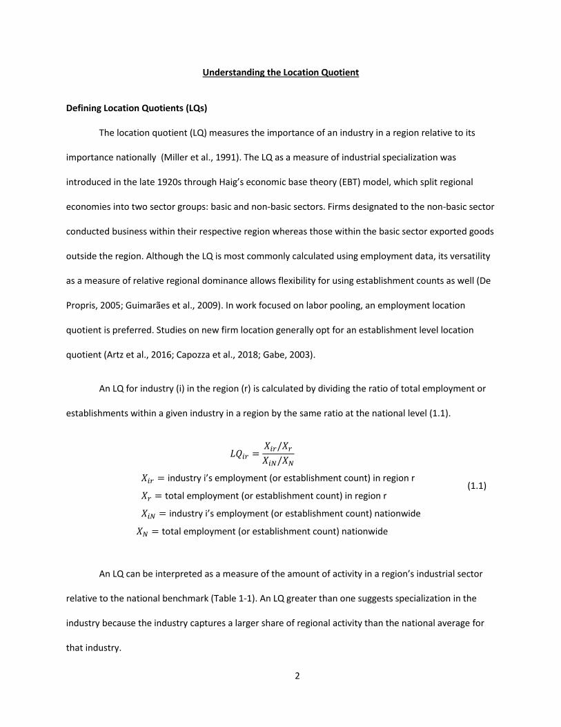
An LQ for industry (i) in the region (r) is calculated by dividing the ratio of total employment or

establishments within a given industry in a region by the same ratio at the national level (1.1).

𝐿𝑄𝑖𝑟 =𝑋𝑖𝑟/𝑋𝑟

𝑋𝑖𝑁/𝑋𝑁

𝑋𝑖𝑟 = industry i’s employment (or establishment count) in region r

𝑋𝑟 = total employment (or establishment count) in region r

𝑋𝑖𝑁 = industry i’s employment (or establishment count) nationwide

𝑋𝑁 = total employment (or establishment count) nationwide

(1.1)

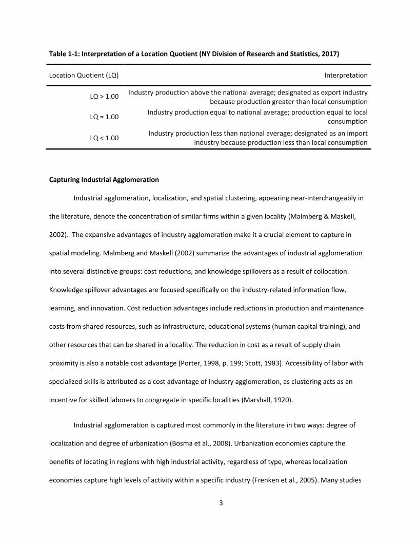
An LQ can be interpreted as a measure of the amount of activity in a region’s industrial sector

relative to the national benchmark (Table 1-1). An LQ greater than one suggests specialization in the

industry because the industry captures a larger share of regional activity than the national average for

that industry.

3

Table 1-1: Interpretation of a Location Quotient (NY Division of Research and Statistics, 2017)

Location Quotient (LQ) Interpretation

LQ > 1.00 Industry production above the national average; designated as export industry because production greater than local consumption

LQ = 1.00 Industry production equal to national average; production equal to local consumption

LQ < 1.00 Industry production less than national average; designated as an import industry because production less than local consumption

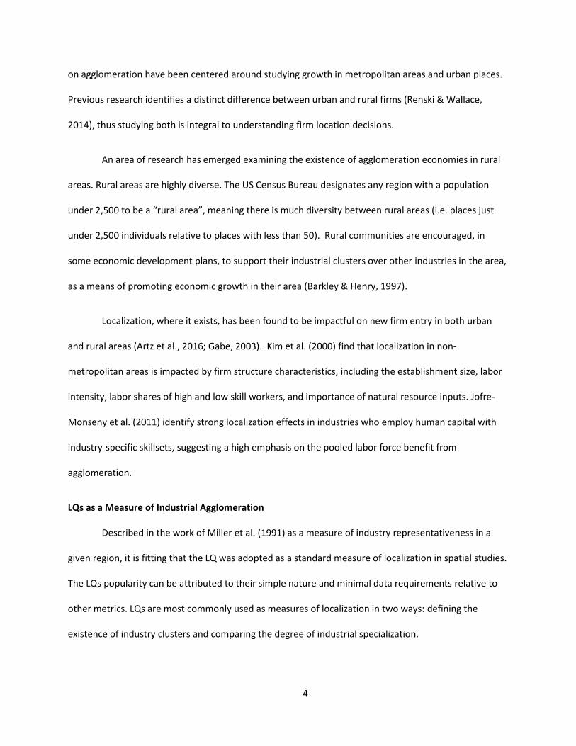
Capturing Industrial Agglomeration

Industrial agglomeration, localization, and spatial clustering, appearing near-interchangeably in

the literature, denote the concentration of similar firms within a given locality (Malmberg & Maskell,

2002). The expansive advantages of industry agglomeration make it a crucial element to capture in

spatial modeling. Malmberg and Maskell (2002) summarize the advantages of industrial agglomeration

into several distinctive groups: cost reductions, and knowledge spillovers as a result of collocation.

Knowledge spillover advantages are focused specifically on the industry-related information flow,

learning, and innovation. Cost reduction advantages include reductions in production and maintenance

costs from shared resources, such as infrastructure, educational systems (human capital training), and

other resources that can be shared in a locality. The reduction in cost as a result of supply chain

proximity is also a notable cost advantage (Porter, 1998, p. 199; Scott, 1983). Accessibility of labor with

specialized skills is attributed as a cost advantage of industry agglomeration, as clustering acts as an

incentive for skilled laborers to congregate in specific localities (Marshall, 1920).

Industrial agglomeration is captured most commonly in the literature in two ways: degree of

localization and degree of urbanization (Bosma et al., 2008). Urbanization economies capture the

benefits of locating in regions with high industrial activity, regardless of type, whereas localization

economies capture high levels of activity within a specific industry (Frenken et al., 2005). Many studies

4

on agglomeration have been centered around studying growth in metropolitan areas and urban places.

Previous research identifies a distinct difference between urban and rural firms (Renski & Wallace,

2014), thus studying both is integral to understanding firm location decisions.

An area of research has emerged examining the existence of agglomeration economies in rural

areas. Rural areas are highly diverse. The US Census Bureau designates any region with a population

under 2,500 to be a “rural area”, meaning there is much diversity between rural areas (i.e. places just

under 2,500 individuals relative to places with less than 50). Rural communities are encouraged, in

some economic development plans, to support their industrial clusters over other industries in the area,

as a means of promoting economic growth in their area (Barkley & Henry, 1997).

Localization, where it exists, has been found to be impactful on new firm entry in both urban

and rural areas (Artz et al., 2016; Gabe, 2003). Kim et al. (2000) find that localization in non-

metropolitan areas is impacted by firm structure characteristics, including the establishment size, labor

intensity, labor shares of high and low skill workers, and importance of natural resource inputs. Jofre-

Monseny et al. (2011) identify strong localization effects in industries who employ human capital with

industry-specific skillsets, suggesting a high emphasis on the pooled labor force benefit from

agglomeration.

LQs as a Measure of Industrial Agglomeration

Described in the work of Miller et al. (1991) as a measure of industry representativeness in a

given region, it is fitting that the LQ was adopted as a standard measure of localization in spatial studies.

The LQs popularity can be attributed to their simple nature and minimal data requirements relative to

other metrics. LQs are most commonly used as measures of localization in two ways: defining the

existence of industry clusters and comparing the degree of industrial specialization.

5

1. Defining the existence of industry clusters

The LQ is often used in congruence to other metrics for identification of industry agglomeration

(i.e. industry clusters). In some studies, the LQ is calculated following a supply-chain analysis of the

region, which allows for a more accurate grouping of clusters that exist outside of industrial groupings

(Delgado et al., 2014a; Maine Center for Business and Economic Research et al., 2008; Resbeut &

Gugler, 2016). When used to define existence of industry clusters, an LQ cutoff is typically implemented.

A value of 1.0 is a commonly implemented, because an LQ greater than 1.0 signifies a greater regional

share in the industry relative to the national level. However, different studies opt for different studies

and this arbitrary use of cutoffs is a common criticism of LQs in the literature (Crawley et al., 2013;

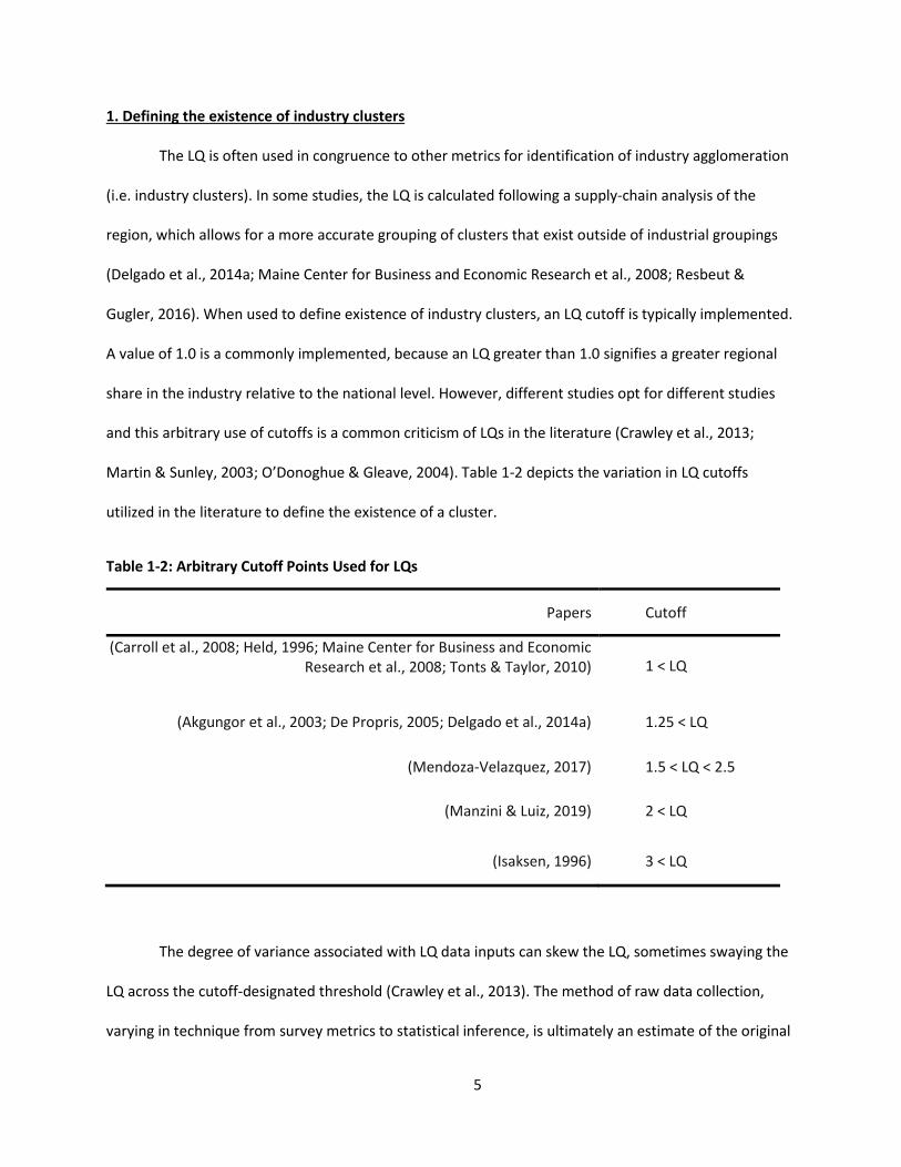
Martin & Sunley, 2003; O’Donoghue & Gleave, 2004). Table 1-2 depicts the variation in LQ cutoffs

utilized in the literature to define the existence of a cluster.

Table 1-2: Arbitrary Cutoff Points Used for LQs

Papers Cutoff

(Carroll et al., 2008; Held, 1996; Maine Center for Business and Economic Research et al., 2008; Tonts & Taylor, 2010)

1 < LQ

(Akgungor et al., 2003; De Propris, 2005; Delgado et al., 2014a) 1.25 < LQ

(Mendoza-Velazquez, 2017) 1.5 < LQ < 2.5

(Manzini & Luiz, 2019) 2 < LQ

(Isaksen, 1996) 3 < LQ

The degree of variance associated with LQ data inputs can skew the LQ, sometimes swaying the

LQ across the cutoff-designated threshold (Crawley et al., 2013). The method of raw data collection,

varying in technique from survey metrics to statistical inference, is ultimately an estimate of the original

6

data. For example, at a low level of industrial aggregation, publicly available employment and

establishment figures for a given year and industry may be imputed estimates rather than direct figures.

It is crucial to consider the degree of variance associated with the LQ data inputs, particularly in small

rural regions comprised of only a handful of establishments, because even miscounting by one company

has the potential has the potential of shifting the size of the LQ over the arbitrary cutoff used to

designate the existence of clustering.

Implementing standardizations and developing indices to overcome scale-sensitivity of the LQ is

an alternative to an arbitrary cutoff (Carroll et al., 2008; Mulligan & Schmidt, 2005; Resbeut & Gugler,

2016). O’Donoghue and Gleave (2004) suggest implementing a standardized location quotient, which

allows significance to be determined across different sample sizes by using a z-score to identify the

appropriate cut-off for the sample. While standardization is able to control for the relative differences

between the regional LQs, this methodology just swaps the use of a numeric cutoff to a proportion of

the sample. Therefore, it is unable to prevent potential misrepresentation that LQs may have at a small

regional level.

2. Comparing the degree of industrial specialization

LQs can be implemented within a spatial model to cross compare industry agglomeration across

sectors and regions, often either as continuous numeric variables or categorical dummies (Artz et al.,

2016; Capozza et al., 2018; Delgado et al., 2014b; Gabe, 2003; Holl, 2004; Mulligan & Schmidt, 2005).

While this method does not require the use of an arbitrary cutoff, this use of the LQ is also subject to

scale sensitivity and data variance problems.

Wennberg and Lindqvist (2010) allude to the LQ’s scale-sensitivity while testing between

absolute and relative measures of agglomeration in their results, suggesting that, despite the LQ’s

strength for cluster identification, it is a weak measure for capturing the effect of variation in cluster

7

strength. Fracasso and Marzetti (2018), on the other hand, conclude the LQ to be an unbiased metric,

but caution that failing to properly control for overall size of local economic activity will result in a

substantial bias. This inability of the LQ to control for absolute size of place can be mitigated through the

use of a standardized location quotient (O’Donoghue & Gleave, 2004) or by comparing the local industry

level to a sample of similarly sized regions, using a technique first introduced by Ullman and Dacey

(1960). However, while Klosterman (1990) notes a benefit of looking at similar sized regions rather than

the nation as a whole gives a fairer comparative, Pratt (1968) describes this technique as weaker than

the traditional LQ.

The data variance limitation of the LQ is more challenging to overcome. The LQ requires single

point-estimates for calculation but does not assess the degree of accuracy of these point estimates,

which are subject to measurement error (Beyene & Moineddin, 2005). Billings and Johnson (2012)

identify a tradeoff between aggregation level and statistical inference precision. The degree of spatial

and industrial aggregation has generally been left up to the discretion of the researcher, with data

availability often acting as the greatest limiting factor. There is no agreement in the literature on the

optimal geographical boundaries. Thus, location studies vary extensively by size of spatial units and by

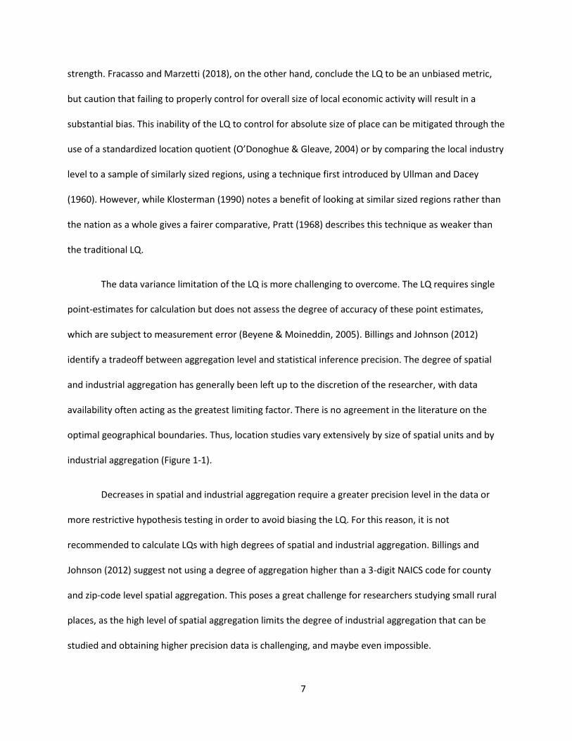
industrial aggregation (Figure 1-1).

Decreases in spatial and industrial aggregation require a greater precision level in the data or

more restrictive hypothesis testing in order to avoid biasing the LQ. For this reason, it is not

recommended to calculate LQs with high degrees of spatial and industrial aggregation. Billings and

Johnson (2012) suggest not using a degree of aggregation higher than a 3-digit NAICS code for county

and zip-code level spatial aggregation. This poses a great challenge for researchers studying small rural

places, as the high level of spatial aggregation limits the degree of industrial aggregation that can be

studied and obtaining higher precision data is challenging, and maybe even impossible.

8

Figure 1-1: LQ Industrial and Spatial Aggregation Levels in Literature

Parsing out the degree to which the data’s variance may be skewing the results is a limitation

that has yet to be overcome in research on agglomeration in small rural places. This work aims to

introduce a simple methodology for testing the robustness of the LQ at a high level of spatial

aggregation

Testing the LQ in Small Rural Places

The construction of the LQ as a relative measure of an industry’s presence in a region compared

with a national benchmark might make it an unreliable indicator of industry localization in small rural

places. When working with small rural places with a limited number of establishments but a small

9

presence in several key industries, a large location quotient may not necessarily be indicative of actual

specialization. A high LQ in such a region might be a true sign of a local industry cluster (e.g. providing

benefits to existing companies and an attraction to new firms), or it might be a “false signal” due to the

presence of one establishment in a small region.

To demonstrate the volatility of the location quotient in a small rural place, consider Table 1-3,

which shows the 20 highest LQs calculated at the town-industry group level in Maine. This table is

obtained from a dataset, described in more detail in the next section, with a high level of spatial

aggregation and a moderate level of industrial aggregation. This dataset is comprised of 6,110 town-

industry pairs: representing 13 industrial groups in 470 towns. The 13 industry groups are aggregated

industry clusters specific to Maine1. (e.g. Environmental Services, Forestry-Related Products, and

Medical Devices), consisting of as few as 3 and as many as 50 six-digit NAICS codes: a moderate level of

industrial aggregation.

Although places with a population of 500 people or fewer represent 25% of towns in the

dataset, they contain 47% of the LQs in Table 1-3. Isle Au Haut, for example, which has a population of

less than 100 people and a total of 8 establishments, is home to the “largest” industrial cluster in the

state. The Isle Au Haut Alternative Energy and Turbines cluster has a specialization 652 times the

national average. In reality, the cluster consists of a single energy company which supplies power to the

island. 65% of the most highly specialized industrial clusters in Table 1-3 consist of a single

establishment. If that one company were to disappear, the LQ would drop from values excess of 100 to

zero. Likewise, the LQ would change dramatically if the cluster were to grow by one establishment or

simply if another establishment were to be added to the town.

1 The industry clusters used in this study are aggregated by Bastille and Maine Technology Technology institute. They represent 13 industry groups that are dominant economic growth industries In the state of Maine.

10

Table 1-3: Top 20 LQs for Maine Town-Industry Groups

LQ Industry Group Town Town Population

Industry Group Establishments

653 Alternative Energy and Turbines Isle au Haut 61 1 574 Boatbuilding and Related Industries Atkinson 249 2 539 Boatbuilding and Related Industries Brooklin 858 7 475 Alternative Energy and Turbines Atkinson 249 1 316 Boatbuilding and Related Industries Cranberry Isles 123 1 263 Boatbuilding and Related Industries Beals 485 1 218 Boatbuilding and Related Industries North Haven 410 2 176 Boatbuilding and Related Industries Long Island 239 1 163 Alternative Energy and Turbines Parsonsfield 1,746 1 159 Alternative Energy and Turbines Arundel 4,100 6

157 Agriculture, Aquaculture, Fisheries and Food Production Westmanland 89 1

148 Forestry-Related Products Carroll plantation 115 1 145 Alternative Energy and Turbines Perry 825 1 142 Boatbuilding and Related Industries Southwest Harbor 1,976 7 132 Boatbuilding and Related Industries Sedgwick 1,137 2 127 Alternative Energy and Turbines Exeter 1,012 1 122 Boatbuilding and Related Industries Steuben 1,017 2 105 Boatbuilding and Related Industries South Bristol 952 1 104 Alternative Energy and Turbines Milford 3,054 1

99 Alternative Energy and Turbines Cushing 1,415 1

To examine the stability of the LQs for the Maine town-industry pairs, an experiment can be

performed where an additional establishment is added to each of the 13 clusters in a given town.

Consider the previously discussed LQ for the Alternative Energy and Turbines cluster in Isle Au Haut. The

breakdown of the LQ calculation is captured in (Equation (1.2).

𝐿𝑄 =𝑋𝑖𝑟/𝑋𝑟

𝑋𝑖𝑁/𝑋𝑁=

1/81,448/7,563,084

= 652.891 (1.2)

Equation (1.3 depicts what would happen to the LQ for the town’s Alternative Energy and Turbines

cluster, if an additional establishment were added to each of the 13 clusters in Isle Au Haut.

11

𝐿𝑄𝑎𝑑𝑗 =(𝑋𝑖𝑟 + 1)/(𝑋𝑟 + 13)(𝑋𝑖𝑁 + 1)/(𝑋𝑁 + 13)

=2/21

1,449/7,563,097= 497.098 (1.3)

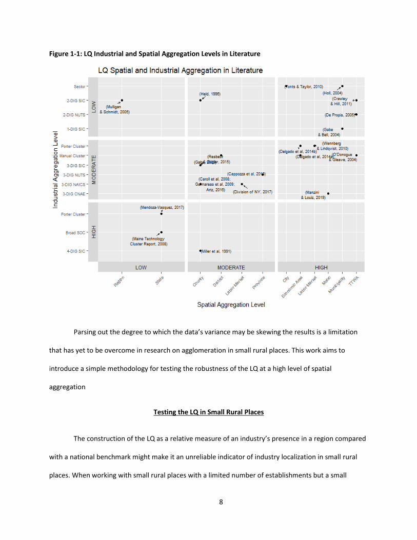
The adjusted LQ is approximately 31% smaller than the initial LQ. The substantial difference between

the original and adjusted LQ calls into question whether reliable information on industrial agglomeration

can be extrapolated at this level of industrial aggregation from Isle Au Haut. Squaring the difference

between the original LQ and the adjusted LQ calculations (Equation 1.3) penalizes the larger differences

in LQs and accounts for both positive and negative changes

𝐷𝑖𝑓𝑓𝑆𝑞 = (𝐿𝑄𝑎𝑑𝑗 − 𝐿𝑄)2 = 24,271.46 (1.4)

Calculating the difference squared for each of the LQs in Isle Au Haut provides a basic overview

of how volatile the LQ calculations are to small changes in establishment counts. Table 1-4 shows the

difference squared for all the industry clusters located on Isle Au Haut.

Table 1-4: Volatility of LQs for Industry Clusters in Isle Au Haut

Industry Cluster LQ adjLQ diffSq Alternative Energy and Turbines 653 497 24,165 Agriculture, Aquaculture, Fisheries and Food Production 20 15 22 Biopharmaceuticals 0 40 1,603 Boatbuilding and Related Industries 0 150 22,631 Defense 0 87 7,630 Electronics and Semiconductors 0 34 1,155 Engineering and Scientific/Technical Services 0 4 18 Environmental Services 0 13 166 Finance and Business Support Services 0 1 1 Forestry-Related Products 0 7 50 Information Technology Services 0 2 5 Materials for Textiles, Apparel, Leather and Footwear 0 9 87 Medical Devices 0 58 3,348

The average difference squared for the LQs across all industry clusters in Isle Au Haut is 4,683, meaning

that on average the LQs for each cluster change by 68 when the clusters are increased by a single

establishment. This suggests that LQs may not be a reliable indicator of industry specialization in this

locality.

12

To examine the stability of the LQs in towns of all sizes, a similar analysis is conducted for all

6,110 town-industry pairs in Maine. Business location data from Dunn and Bradstreet (D&B) dataset is

used to obtain company counts at a town level for each of the 13 aggregated industry sectors2. An LQ is

calculated for each sector and region: the numerator is comprised of D&B companies founded in 2014

or earlier and the denominator using 2014 US level industry data (Equation (1.5).

𝐿𝑄𝑐𝑟 =𝑋𝑐𝑟/𝑋𝑟

𝑋𝑐𝑁/𝑋𝑁 (1.5)

Next, an adjusted location quotient is calculated for each sector and region by adding a single new

company in each sector to each region (Equation (1.6).

𝐿𝑄𝑎𝑑𝑗 =(𝑋𝑐𝑟 + 1)/(𝑋𝑟 + 13)(𝑋𝑐𝑁 + 1)/(𝑋𝑁 + 13)

(1.6)

Lastly, the average difference squared between the original and adjust LQ is used to test the robustness

of the LQs in each region (Equation (1.7).

𝐴𝑣𝐷𝑖𝑓𝑓𝑆𝑞 =∑ (𝑐 𝐿𝑄𝑎𝑑𝑗 − 𝐿𝑄)2

13 (1.7)

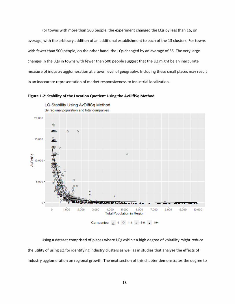
Figure 1-2 shows the average stability of the LQ for each region, captured by AvDiffSq, relative

to the size of the region. As the size of the region increases, in both population and number of

companies, the volatility of the LQ decreases to zero. For rural regions (i.e towns with a population less

than 2500), there is always some degree of volatility with the LQ, compared to urban regions. The

smaller the region the more unstable the LQ becomes.

2 The D&B data for Maine consists of 57,735 establishments, 6747 (11%) of which are in one of the 13 aggregated industry sectors. Of the 6,747 establishments, 5,821 (86%) were founded prior to 2014.

13

For towns with more than 500 people, the experiment changed the LQs by less than 16, on

average, with the arbitrary addition of an additional establishment to each of the 13 clusters. For towns

with fewer than 500 people, on the other hand, the LQs changed by an average of 55. The very large

changes in the LQs in towns with fewer than 500 people suggest that the LQ might be an inaccurate

measure of industry agglomeration at a town level of geography. Including these small places may result

in an inaccurate representation of market responsiveness to industrial localization.

Figure 1-2: Stability of the Location Quotient Using the AvDiffSq Method

Using a dataset comprised of places where LQs exhibit a high degree of volatility might reduce

the utility of using LQ for identifying industry clusters as well as in studies that analyze the effects of

industry agglomeration on regional growth. The next section of this chapter demonstrates the degree to

14

which including LQs from high-volatility places alters the market responsiveness to agglomeration in a

model analyzing location decisions of business in Maine.

Industrial Clustering and Innovation in Maine

The extensive benefits of regional agglomeration, such as knowledge sharing and cost

reductions from shared resources, supply chain proximity, and labor pooling, serve as an incentive for

new firm entry (Malmberg & Maskell, 2002; Marshall, 1920; Porter, 1998; Scott, 1983). Within-industry

agglomeration (i.e. localization) has been found linked to increased entrepreneurship, a benefit of

knowledge-sharing (Nyström, 2005). Localization in industries with an industry-specific labor force

suggests a demand for labor pooling as well (Jofre-Monseny et al., 2011). Understanding the link

between agglomeration and new firm entry for the state of Maine could help inform policy decisions to

help improve Maine’s economic well-being.

Previously, localization economies and their effect on new firm formation has been studied at a

county level in Maine (Gabe, 2003; Gabe & Bell, 2004). However, it is bold to assume that industrial

composition of the towns within each Maine county is homogenous. For example, Aroostook county,

the largest and northernmost county in Maine, is the size of Connecticut and Rhode Island combined.

However, studying localization at a higher level of spatial aggregation would require a more cautious

approach to the measures used to model it. Using LQs to measure localization without controlling for

their volatility in some places may mask the effect of localization on firm location decisions. The effect of

the small places with volatile LQs on modeling the relationship between industrial agglomeration and

new firm location is demonstrated through the creation of a model for the number of new business

startups in Maine towns.

15

Data

A dataset is constructed for every Census county-subdivision in Maine capturing new business

entry in the 13 technology clusters recognized by the Maine Technology Institute (MTI) based on various

characteristics. The dataset is comprised of data from 5 different sources, matched based on common

identifiers (Figure 1-3).

Figure 1-3: Maine Innovation Model Data Flow Chart

Business location data from a 2017 Dunn and Bradstreet (D&B) dataset is used to obtain

company count data on Maine’s businesses. Company counts are filtered into the 13 technology clusters

in Maine, as recognized by the Maine Technology Institute (MTI) and Battelle (Table 1-5). These clusters

consist of as few as three 3 and as many as 50 six-digit NAICS codes, based on mutual supply chains,

technological competencies, markets, and their role in the state’s economy (Battelle Technology

Partnership Practice, 2014). D&B companies within Maine’s innovative clusters are divided into two

16

groups based on the date they were founded: new companies (founded in 2014 or later) and existing

companies (founded prior to 2014). Regional characteristics and fiscal policy data on the Census county

subdivisions are obtained from the American Community Survey (ACS) and the State of Maine for the

year 2014, to control for conditions at the time of entry.

Table 1-5: Companies Founded Before 2014 by Maine Technology Cluster

Maine Technology Cluster Total Companies Agriculture, Aquaculture, Fisheries and Food Production 1933

Alternative Energy and Turbines 92 Biopharmaceuticals 62

Boatbuilding and Related Industries 100 Defense 29

Electronics and Semiconductors 51 Engineering and Scientific/Technical Services 488

Environmental Services 428 Finance and Business Support Services 1814

Forestry-Related Products 658 Information Technology Services 486

Materials for Textiles, Apparel, Leather and Footwear 187 Medical Devices 54

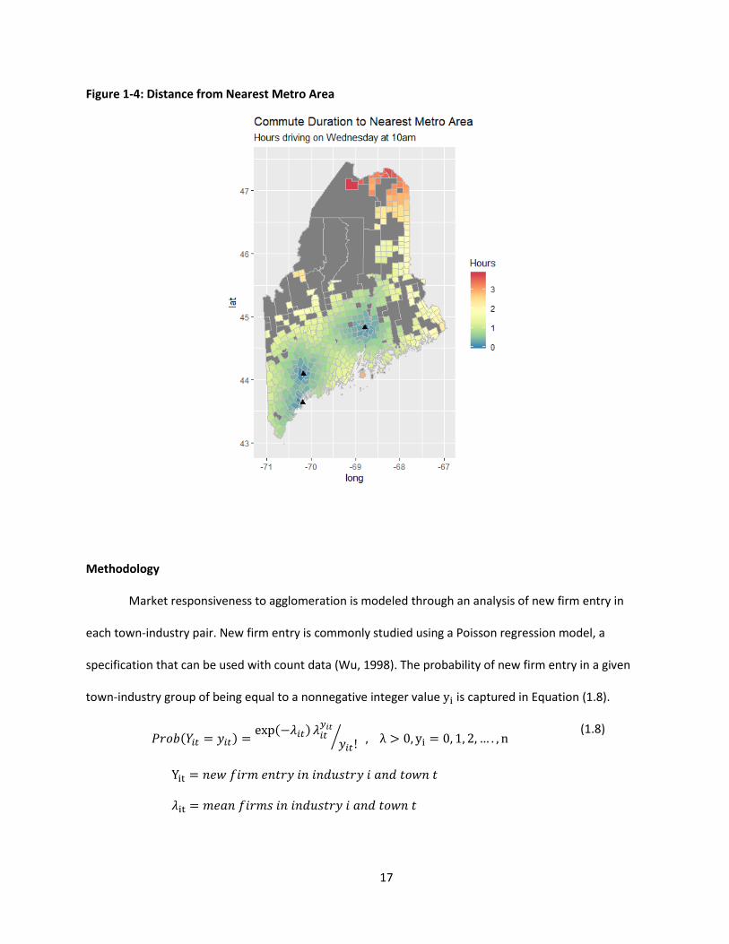
To further control for spatiality, distance to the nearest metropolitan area (i.e. Portland,

Lewiston, and Bangor) are calculated using the Google API mapping software. The distances are

calculated from the centroid of each town in minutes it would take to drive there on a Wednesday at

10am. Figure 1-4 graphically shows the commute distance, rounded up to hours, for each of the towns

in the dataset

17

Figure 1-4: Distance from Nearest Metro Area

Methodology

Market responsiveness to agglomeration is modeled through an analysis of new firm entry in

each town-industry pair. New firm entry is commonly studied using a Poisson regression model, a

specification that can be used with count data (Wu, 1998). The probability of new firm entry in a given

town-industry group of being equal to a nonnegative integer value yi is captured in Equation (1.8).

𝑃𝑟𝑜𝑏(𝑌𝑖𝑡 = 𝑦𝑖𝑡) = exp(−𝜆𝑖𝑡) 𝜆𝑖𝑡𝑦𝑖𝑡

𝑦𝑖𝑡! ⁄ , λ > 0, yi = 0, 1, 2, … . , n

Yit = 𝑛𝑒𝑤 𝑓𝑖𝑟𝑚 𝑒𝑛𝑡𝑟𝑦 𝑖𝑛 𝑖𝑛𝑑𝑢𝑠𝑡𝑟𝑦 𝑖 𝑎𝑛𝑑 𝑡𝑜𝑤𝑛 𝑡

𝜆it = 𝑚𝑒𝑎𝑛 𝑓𝑖𝑟𝑚𝑠 𝑖𝑛 𝑖𝑛𝑑𝑢𝑠𝑡𝑟𝑦 𝑖 𝑎𝑛𝑑 𝑡𝑜𝑤𝑛 𝑡

(1.8)

18

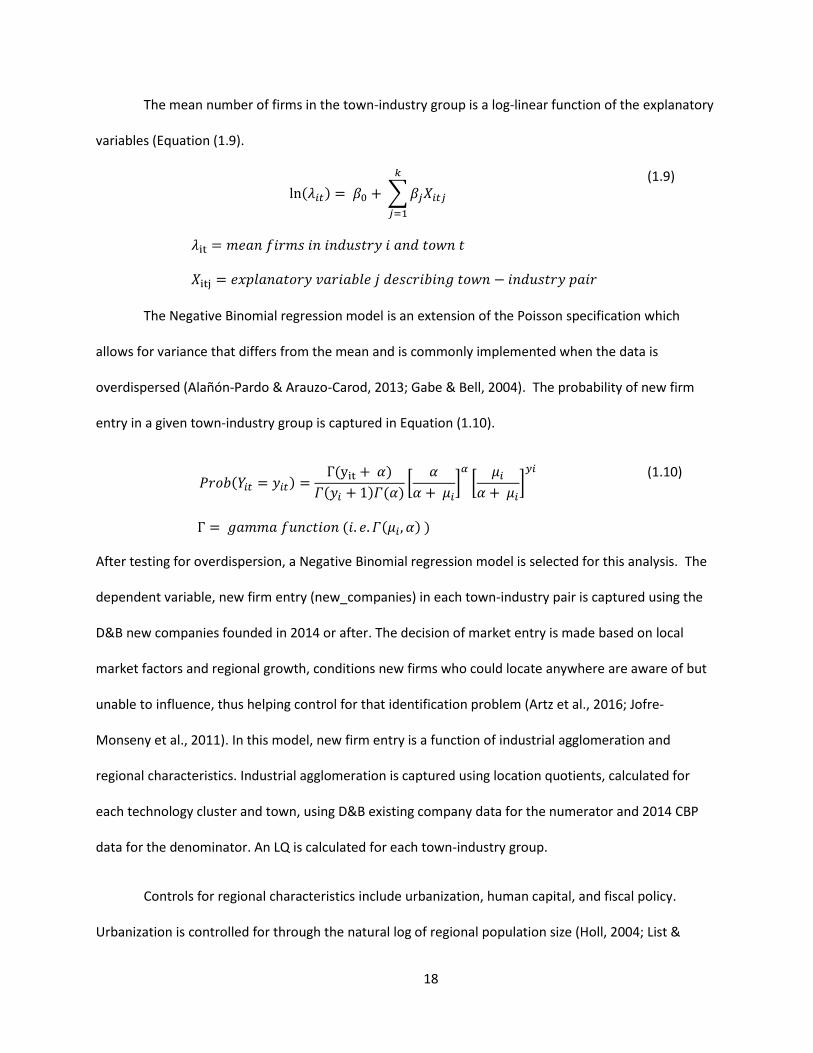
The mean number of firms in the town-industry group is a log-linear function of the explanatory

variables (Equation (1.9).

ln(𝜆𝑖𝑡) = 𝛽0 + ∑ 𝛽𝑗𝑋𝑖𝑡𝑗

𝑘

𝑗=1

𝜆it = 𝑚𝑒𝑎𝑛 𝑓𝑖𝑟𝑚𝑠 𝑖𝑛 𝑖𝑛𝑑𝑢𝑠𝑡𝑟𝑦 𝑖 𝑎𝑛𝑑 𝑡𝑜𝑤𝑛 𝑡

𝑋itj = 𝑒𝑥𝑝𝑙𝑎𝑛𝑎𝑡𝑜𝑟𝑦 𝑣𝑎𝑟𝑖𝑎𝑏𝑙𝑒 𝑗 𝑑𝑒𝑠𝑐𝑟𝑖𝑏𝑖𝑛𝑔 𝑡𝑜𝑤𝑛 − 𝑖𝑛𝑑𝑢𝑠𝑡𝑟𝑦 𝑝𝑎𝑖𝑟

(1.9)

The Negative Binomial regression model is an extension of the Poisson specification which

allows for variance that differs from the mean and is commonly implemented when the data is

overdispersed (Alañón-Pardo & Arauzo-Carod, 2013; Gabe & Bell, 2004). The probability of new firm

entry in a given town-industry group is captured in Equation (1.10).

𝑃𝑟𝑜𝑏(𝑌𝑖𝑡 = 𝑦𝑖𝑡) =Γ(yit + 𝛼)

𝛤(𝑦𝑖 + 1)𝛤(𝛼) [𝛼

𝛼 + 𝜇𝑖]

𝛼[

𝜇𝑖

𝛼 + 𝜇𝑖]

𝑦𝑖

Γ = 𝑔𝑎𝑚𝑚𝑎 𝑓𝑢𝑛𝑐𝑡𝑖𝑜𝑛 (𝑖. 𝑒. 𝛤(𝜇𝑖, 𝛼) )

(1.10)

After testing for overdispersion, a Negative Binomial regression model is selected for this analysis. The

dependent variable, new firm entry (new_companies) in each town-industry pair is captured using the

D&B new companies founded in 2014 or after. The decision of market entry is made based on local

market factors and regional growth, conditions new firms who could locate anywhere are aware of but

unable to influence, thus helping control for that identification problem (Artz et al., 2016; Jofre-

Monseny et al., 2011). In this model, new firm entry is a function of industrial agglomeration and

regional characteristics. Industrial agglomeration is captured using location quotients, calculated for

each technology cluster and town, using D&B existing company data for the numerator and 2014 CBP

data for the denominator. An LQ is calculated for each town-industry group.

Controls for regional characteristics include urbanization, human capital, and fiscal policy.

Urbanization is controlled for through the natural log of regional population size (Holl, 2004; List &

19

McHone, 2000). Human capital heterogeneity is captured through a measure of the concentration of

college graduates in the region (ed_higher_p) (Arauzo-Carod et al., 2010; Artz et al., 2016). Fiscal policy,

shown to be impactful on new firm location, are included in the form of tax rate (taxrate) and per capita

government expenditure (govspending) (Gabe & Bell, 2004; Head et al., 1999). Dummy variables for

each innovative cluster are included to control for variation across innovative cluster on the impact of

agglomeration on new firm entry. Location quotients are interacted with the dummies to identify the

marginal effects. County-level dummies and the distance to the nearest municipality (distmun) are

included to control for spatiality.

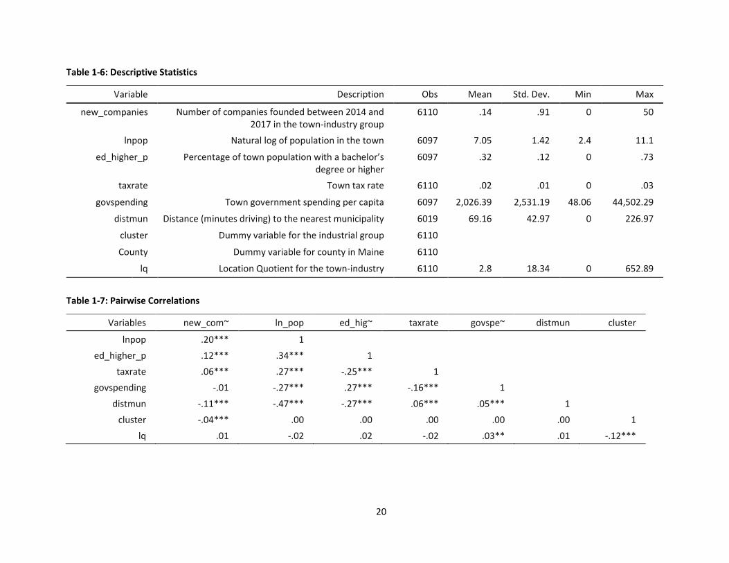
Summary statistics and variable descriptions for model variables are shown in Table 1-6 and

pairwise correlations between the variables in Table 1-7.

20

Table 1-6: Descriptive Statistics

Variable Description Obs Mean Std. Dev. Min Max

new_companies Number of companies founded between 2014 and 2017 in the town-industry group

6110 .14 .91 0 50

lnpop Natural log of population in the town 6097 7.05 1.42 2.4 11.1

ed_higher_p Percentage of town population with a bachelor’s degree or higher

6097 .32 .12 0 .73

taxrate Town tax rate 6110 .02 .01 0 .03

govspending Town government spending per capita 6097 2,026.39 2,531.19 48.06 44,502.29

distmun Distance (minutes driving) to the nearest municipality 6019 69.16 42.97 0 226.97

cluster Dummy variable for the industrial group 6110

County Dummy variable for county in Maine 6110

lq Location Quotient for the town-industry 6110 2.8 18.34 0 652.89

Table 1-7: Pairwise Correlations

Variables new_com~ ln_pop ed_hig~ taxrate govspe~ distmun cluster

lnpop .20*** 1 ed_higher_p .12*** .34*** 1

taxrate .06*** .27*** -.25*** 1 govspending -.01 -.27*** .27*** -.16*** 1

distmun -.11*** -.47*** -.27*** .06*** .05*** 1 cluster -.04*** .00 .00 .00 .00 .00 1

lq .01 -.02 .02 -.02 .03** .01 -.12***

21

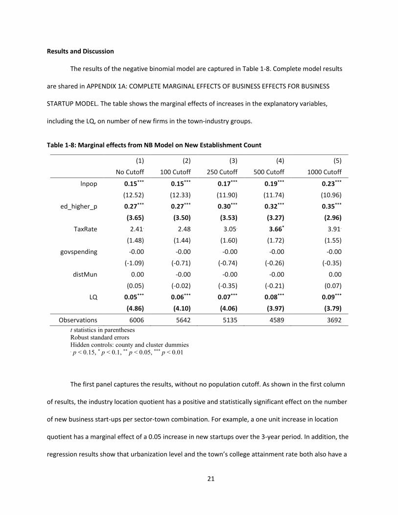
Results and Discussion

The results of the negative binomial model are captured in Table 1-8. Complete model results

are shared in APPENDIX 1A: COMPLETE MARGINAL EFFECTS OF BUSINESS EFFECTS FOR BUSINESS

STARTUP MODEL. The table shows the marginal effects of increases in the explanatory variables,

including the LQ, on number of new firms in the town-industry groups.

Table 1-8: Marginal effects from NB Model on New Establishment Count

(1) (2) (3) (4) (5) No Cutoff 100 Cutoff 250 Cutoff 500 Cutoff 1000 Cutoff

lnpop 0.15*** 0.15*** 0.17*** 0.19*** 0.23*** (12.52) (12.33) (11.90) (11.74) (10.96)

ed_higher_p 0.27*** 0.27*** 0.30*** 0.32*** 0.35*** (3.65) (3.50) (3.53) (3.27) (2.96)

TaxRate 2.41. 2.48 3.05. 3.66* 3.91. (1.48) (1.44) (1.60) (1.72) (1.55)

govspending -0.00 -0.00 -0.00 -0.00 -0.00 (-1.09) (-0.71) (-0.74) (-0.26) (-0.35)

distMun 0.00 -0.00 -0.00 -0.00 0.00 (0.05) (-0.02) (-0.35) (-0.21) (0.07)

LQ 0.05*** 0.06*** 0.07*** 0.08*** 0.09*** (4.86) (4.10) (4.06) (3.97) (3.79)

Observations 6006 5642 5135 4589 3692 t statistics in parentheses Robust standard errors Hidden controls: county and cluster dummies . p < 0.15, * p < 0.1, ** p < 0.05, *** p < 0.01

The first panel captures the results, without no population cutoff. As shown in the first column

of results, the industry location quotient has a positive and statistically significant effect on the number

of new business start-ups per sector-town combination. For example, a one unit increase in location

quotient has a marginal effect of a 0.05 increase in new startups over the 3-year period. In addition, the

regression results show that urbanization level and the town’s college attainment rate both also have a

22

positive effect on number of new business startups. A percentage point increase in population size

increases the number of new establishments in the town-cluster group by 0.15, whereas the proportion

of the population with a college degree or higher increases the number of new establishments in the

town-cluster group by 0.27.

In order to examine the influence of including observations from very small places, where the

LQ may be an unreliable indicator of local industry specialization, the business start-up model is re-

estimated using several population cut-off thresholds. For example, a population cut-off of 100 people

removes from the sample the 32 smallest places in Maine (6.8% of the dataset), whereas a cut-off of

1,000 people removes 186 places in Maine (39.6% of the dataset). Panels 2 – 5 compare marginal effects

to the business startup model when population cutoffs are implemented in the highly-volatile LQ range

of under 1,000 people that was depicted in Figure 1-2. The highly educated proportion of the labor

force, urbanization, and industrial localization of the region remain significant in all iterations of the

model. The standard errors for all the significant coefficients decrease as larger population cutoffs are

implemented.

The LQ is significant at a 1%, regardless of cutoff level, however, the significant of the coefficient

increases as the cutoff is introduced. With no cutoff implementation, a 1 unit increase in LQ increases

the number of companies founded in a cluster town pairing by 0.05. Implementing a population cutoff

of 100, increases the effect by 0.01. At a population cutoff of 1,000, the population cutoff at which the

average difference squared begins to level out in Figure 1-3, a one unit increase in LQ increases the

number of companies founded in the town-cluster pairing by 0.09.

23

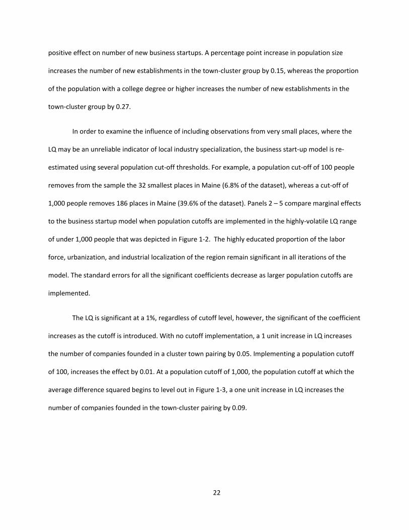
Figure 1-5: Agglomeration Coefficient by Population Cutoff

Observing this effect over a span of cutoffs increasing by increments of 25 yields an interesting

result (Error! Reference source not found.). As the cutoff increases, the marginal effect of the LQ

Coefficient also increases. However, at a population cutoff of about 2,000, the significance level begins

to decrease. This is because the size of the sample decreases to the point where statistical inference

becomes more challenging (Error! Not a valid bookmark self-reference.). Identifying an appropriate

cutoff point requires a balance between removing regions that are too small and ensuring that the

sample still contains enough observations to remain meaningful.

24

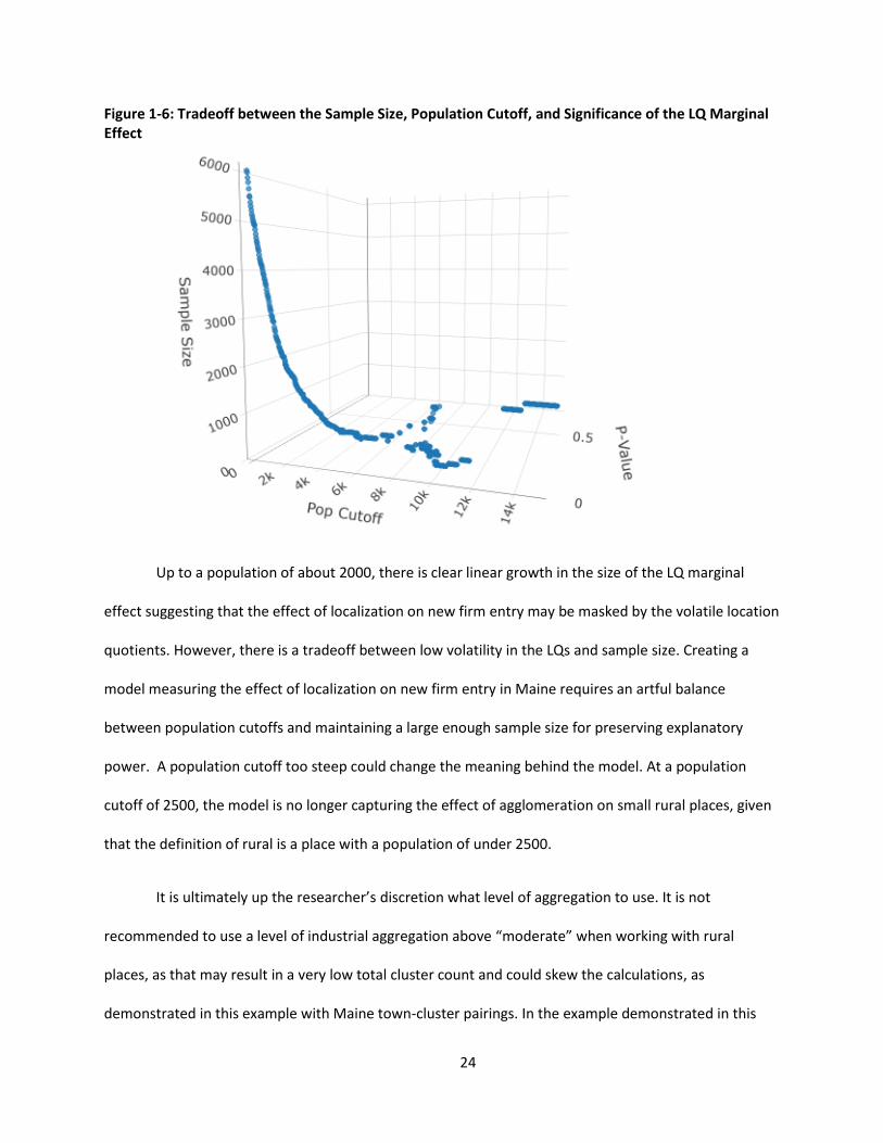
Figure 1-6: Tradeoff between the Sample Size, Population Cutoff, and Significance of the LQ Marginal Effect

Up to a population of about 2000, there is clear linear growth in the size of the LQ marginal

effect suggesting that the effect of localization on new firm entry may be masked by the volatile location

quotients. However, there is a tradeoff between low volatility in the LQs and sample size. Creating a

model measuring the effect of localization on new firm entry in Maine requires an artful balance

between population cutoffs and maintaining a large enough sample size for preserving explanatory

power. A population cutoff too steep could change the meaning behind the model. At a population

cutoff of 2500, the model is no longer capturing the effect of agglomeration on small rural places, given

that the definition of rural is a place with a population of under 2500.

It is ultimately up the researcher’s discretion what level of aggregation to use. It is not

recommended to use a level of industrial aggregation above “moderate” when working with rural

places, as that may result in a very low total cluster count and could skew the calculations, as

demonstrated in this example with Maine town-cluster pairings. In the example demonstrated in this

25

chapter, a moderate level of industrial aggregation and high level of regional aggregation, an average

difference squared of under 1500 for all regions required a population cutoff of 1000, resulting in a

38.5% decrease in sample size but increasing the effect of localization on new firm entry by 4

percentage points. A more volatility-tolerant cutoff of 500 resulted in a decrease in sample size of

23.6% but an increase in the effect of localization on new firm entry of 3 percentage points.

Some rural economic development plans recommend prioritizing investment of public funds in

industrial clusters over other industries as a means of promoting economic growth in the region (Barkley

& Henry, 1997). For small towns in Maine, the policy implications of identifying a strong effect between

localization and new firm entry could include shifting investments to support an entirely different set of

industries. Controlling for the highly volatile LQs resulted in an increase in localization effect of 80%. This

is significant when making policy decisions regarding supporting industrial clusters.

Conclusion

This paper provides an overview of location quotients (LQs) as a measure of localization and

discusses the caveats of using LQs in economic modeling when working with small rural places. This

paper demonstrates a methodology for testing the robustness of an LQ for small rural places by adding

an arbitrary company to each industry and recalculating the LQ for each town-industry pair, determining

whether or not the town should be included by examining the average difference squared between the

two LQ calculations. The paper then demonstrated the usefulness of this robustness check, showing that

at moderate level of industrial aggregation and high level of regional aggregation, the effect of

localization on new firm entry could range anywhere from 5 percentage points to over 10 percentage

points, depending on the population cutoff that was implemented. By using average difference squared

to guide the population cutoff decision that both minimizes LQ volatility and maximizes sample size, the

skew associated with LQs for small rural places can be minimized.

26

The findings in this paper contribute to the literature by providing a simple robustness check for

location quotients when working with small rural places. A preliminary examination of the data, with an

implementation of the average difference squared method, and a check of model results by varying

population cutoffs, as demonstrated in this chapter, may help assess and control for the volatility of LQs.

Given the policy implications of findings regarding industrial clusters and regional economic growth,

ensuring that the results capture the true effect and not a biased one is crucial to the success and

prosperity of these regions.

27

CHAPTER 2

2. THE ROLE OF REGIONAL AGGLOMERATION AS A DETERMINANT OF EDUCATIONAL MISMATCH

IN COLLEGE GRADUATES

In 2018, 32% of United States residents over the age of 18 have completed a bachelor’s degree

or higher: the highest educational attainment in the country to date (CPS, 2018). Yet, as educational

levels continue to rise, overeducation, a form of educational mismatch categorizing individuals

employed in fields that require a lower level of degree than they attained, is becoming an ever more

prevalent problem in labor markets across the world (P. J. Sloane et al., 1999; Tsang & Levin, 1985;

Wronowska, 2017).

Regional and urban economists have documented a variety of benefits associated with large

urban areas. Duranton and Puga (2003) classify the sources of these benefits using a typology of sharing,

matching and learning. A key aspect of the urbanization benefit of matching is that large urban areas

provide a thick labor market that helps workers find a job that provides a good match to their skills and

education. Several empirical studies have examined the role of urbanization on labor market job

matching (Abel & Deitz, 2015; Büchel & Battu, 2003; Büchel & van Ham, 2003).

By using data from a 2020 survey of University of Maine alumni, this chapter aims to strengthen

the understanding of the relationship between a region’s size and labor market match. This paper adds

to previous literature by expanding upon the size of place parameter in the data: looking at both small

and large counties. A stronger understanding of the determinants of job matches in college graduates

can be beneficial not only to college students, who aim to graduate and enter the labor force, but also

to institutions for improving the educational foundations and job-prospects of their programs.

28

Educational Mismatch in the Literature

Educational mismatch, defined as the lack of a match between a laborer’s educational

attainment level and the job’s educational requirements, was first introduced to labor economics by

Freeman (1976). Educational mismatch in college graduates is most commonly evaluated at degree level

(Abel & Deitz, 2015; Groot & Maassen van den Brink, 2000; McGoldrick & Robst, 1996; Peter J. Sloane,

2014) but can also be evaluated at more specific college field of study (i.e. college major) level (Abel &

Deitz, 2015; Marin & Hayes, 2017; Robst, 2008). While educational mismatch encapsulates both

undereducation and overeducation, educational mismatch in college graduates is almost exclusively the

latter. In this paper, educational mismatch refers to the overeducation of individuals at a degree-level

and job match captures the inverse, or lack of, overeducation.

Educational mismatch in college graduates has been studied in nations across the world, with

the majority of the studies concentrated in the European Union (Croce & Ghignoni, 2015; Davia et al.,

2017; Dolton et al., 2001; Morgado et al., 2016; Reimer et al., 2008), but representation in the US (Abel

& Deitz, 2015; Clark et al., 2017; Freeman, 1976), Russia (Kyui, 2010; Shevchuk et al., 2015), Australia

(Peter J. Sloane, 2014) and other nations as well. While the studies on educational mismatch span

numerous counties, encompass various calculations of overeducation, and analyze both time series and

panel data, there is consistency across the causes, determinants, and consequences of educational

mismatch. To better understand the link between spatiality and educational mismatch in college

graduates, this chapter will first discuss the methods used to measure educational mismatch, review the

theories for why it takes place, and discuss the determinants of educational mismatch and their

relationship with spatiality. Finally, the literature review concludes with an overview of the

consequences of educational mismatch and how to measure those consequences.

29

Measuring Educational Mismatch:

Educational mismatch and skill information can be captured using objective methods, subjective

methods or a combination of both (Flisi et al., 2017). Objective methods, such as normative job analysis

or statistical realized matches, utilize information exogenous to the data to categorize the educational

requirements for occupations.

A normative job analysis is a formal analysis conducted by a job specialist where the required

level of education is determined for each occupational job classification, such as what is done to create

the Dictionary of Occupational Titles. Overeducation or educational mismatch is represented by a lower

educational requirement for this job than is attained by the individual. Statistical realized matches, on

the other hand, aggregates data on workers in a given occupation and determines the required level of

education based on the average educational requirement of the workers in that job (Hartog, 2000;

Morgado et al., 2016). Subjective methods of measuring overeducation include self-assessment and

self-reporting and are solely dependent on worker-provided information. These self-assessments

require workers to identify either directly the level of education that they think is necessary for their job

or indirectly whether they believe their level of education is suitable to their job.

While less objective than the job analysis or statistical realized matches methods, self-

assessment methods do not require the use of third party analysis and can sometimes be better fitted in

explaining educational requirements for some occupations that have a high variance in day to day tasks

and requirements (Flisi et al., 2017; Hartog, 2000; Morgado et al., 2016). Furthermore, in an extensive

cross-country comparison of overeducation measures in European studies, Capsada-Munsech (2019)

finds that the worker self-assessment, compared to normative job analysis and realized matches

methods, was the only method to consistently and reliably capture overeducation rates across countries

and capture the explanatory power of overeducation.

30

Causes of Educational Mismatch:

There are several key hypotheses explaining the causes of educational mismatch. According to

the theory of career mobility, educational mismatch is a short-term phenomenon at the begining of a

career, where individuals starting out their career may have a higher likelihood of being overeducated

(Sicherman & Galor, 1990). Evaluations of the theory of career mobility are most accurately conducting

using time series data, due to the advantage of following an individual through their career path, but can

be captured in cross-sectional data using number of years since graduation as a proxy for an individual’s

experience in their career. There are mixed results on this hypothesis and multiple empirical studies

found that the employment mismatch remained persistent years after career start and a lack of

evidence of improvement with career transitions (Büchel & Mertens, 2004; P. J. Sloane et al., 1999). The

advancement hypothesis, developed by Büchel and Mertens (2004) to explain the persistence of wage

penalty of overeducation, suggests that overreduction might be prompted by a lack of opportunities for

advancement in their field or place of work.

The heterogeneity hypothesis suggests that the increase in educational attainment and wider

availability of college education has resulted in larger variation in ability and skillset of graduates

(Chevalier, 2003). In traditional theory, workers are treated as homogenous but more recent theoretical

models examining overqualification and overeducation allowed heterogeneity in these areas with

endogenous worker skills and job skill requirements (Albrecht & Vroman, 2002; Dolado et al., 2009).

Heterogeneity across employers and job applicant characteristics has been shown to impact job

matching.

A supply and demand imbalance theory for educational mismatch suggests that there is a

mismatch in educational skillset demanded in the labor market, where there are too many college

graduates searching for employment in positions with too low a demand for college-graduate skilled

31

labor (Tsang & Levin, 1985; Vedder et al., 2013). Croce and Ghignoni (2012) evaluate the effect of this

mismatch on labor market matching in Europe, finding evidence to reject this theory but identify a

relationship between regional labor market conditions and overeducation. The policy recommendation

from this finding is centered on providing assistance to overeducated workers in labor relocation in

addition to supporting the unemployed labor force. The imbalance of supply and demand can be

evaluated through a spatial lens, where willingness to relocate, commuting ability, size, and

specialization of the labor market may increase the likelihood of match by expanding the demand for

labor.

Determinants of Educational Mismatch:

Previous empirical work has identified a strong relationship between regional characteristics

and educational mismatch (Abel & Deitz, 2015; Davia et al., 2017; Fedorets et al., 2019), however, the

relationship is interlinked with, or reliant on controlling for, other determinants of overeducation such

as educational, individual, and employment characteristics. These studies typically focus on regional

characteristics such as population size, labor market characteristics, industrial composition, or proximity

to metropolitan areas. For example, a region’s population size, a proxy for urbanization, might be an

important factor affecting a person’s labor market match because large cities provide thick labor

markets with jobs across the entire spectrum of skills and educational attainment.

Educational characteristics, such as degree attained and field of study, can be a contributor to

educational mismatch. A higher degree level, such as a master’s degree or PhD relative to a bachelor’s

degree, has been found to increase likelihood of job match (Robst, 2007). The field of study of an

individual impact the likelihood of overeducation due to the relationship between field of study and

labor market outcomes (Hansen, 2001; Rossen et al., 2019; van de Werfhorst & Kraaykamp, 2001). Field

of studies differ by occupational focus, transitivity of skill to the workplace, and job-specificity (Ortiz &

32

Kucel, 2008; Reimer et al., 2008). For example, an engineering degree may provide a more direct path

and set of skills to employment as an engineer, thus decreasing the likelihood of overeducation. Otiz and

Kucel (2008) find that services and human arts fields of studies are most likely to exhibit overeducation,

relative to the base category of social sciences, business and law.

Employment characteristics are found in the literature to be impactful on likelihood of

educational mismatch. The direct relationship between college major and occupation-educational

mismatch identified in the literature also suggests that certain occupations might experience higher

overeducation rates than others due to that skill transitivity. Occupations with an excess supply of

college-graduated workers have been shown to require higher field-specific skillset to achieve matching

(Humburg et al., 2017). Other studies also examined the impact of characteristics, such as phrasing of

the job-title, applicant characteristics, such as entrepreneurial skills have on job outcomes and applicant

quality in job matching (Abel & Deitz, 2015; Kucel et al., 2016; Marinescu & Wolthoff, 2019). Sector of

employment has an impact on overeducation, where public sector employment has a lower risk of

overeducation than private sector (Barone & Ortiz Gervasi, 2010; Wolbers, 2003).

As suggested by the heterogeneity hypothesis, variation in individual characteristics, such as

skillset and demographics, can be a determinant of educational mismatch. Educational mismatch is not

synonymous with a skill mismatch, which is a mismatch between the skills required for a given job rather

than a mismatch between the educational credentials, because skill level can fluctuate with built and

lost skillsets. Educational mismatch can contribute extensively to skill mismatch (Flisi et al., 2017; Peter

J. Sloane, 2014; Wronowska, 2017).

Demographic characteristics, such as marital status and gender are all found to be impactful on

educational mismatch. Those who have never been married have been shown to be less likely to be

overeducated (Robst, 2008). The socio-economic impacts of overeducation, such as perceived job

33

mobility, job satisfaction, and wages, are shown in some studies to be exacerbated in women, especially

if they are caregivers to young children (Castagnetti et al., 2018; Shevchuk et al., 2015).

A spatial theory explaining educational mismatch, known as the theory of differential

overqualification, emerged in the work of Frank (1978), theorizing that a family unit’s global market is

determined by the husband’s employment, restricting married women to act as ‘tied movers’ or ‘tied

stayers’ with employment prospects limited to their local region. Based on the theory of differential

overqualification, size of place would have a strong link with overeducation, since smaller labor markets

would provide fewer matching opportunities. McGoldrick & Robst (1996) find results disproving this

theory using US data. Büchel & Battu (2003) incorporate commuting distance into their analysis, finding

that, while married women run a higher likelihood of overeducation in small localities, controlling for

commuting ability through the distance of commute shows that both women and men (to a smaller

degree) are more likely to be overeducated in small localities.

There are mixed findings on whether women more likely to be overeducated (Battu et al., 2000;

McGoldrick & Robst, 1996) or less likely (Castagnetti et al., 2018). Ramos and Sanromá, (2013) find that

gender differences are not significant determinants of overeducation, controlling for all other factors.

However, there are gender differences in the relationship between field of study and overeducation,

where self- selection due to gender norms results in an unequal distribution of males and females in

different fields (Attanasio & Kaufmann, 2017; McGoldrick & Robst, 1996; Zhao et al., 2017).

Rossen et al. (2019) find that male graduates in the services, natural sciences, and agriculture

fields of study were most likely to be overeducated, relative to the social sciences, journalism and

information field of study, whereas those in health and welfare, education, engineering, and arts and

humanities were less likely to be overeducated. Due to the systematic differences in educational and

occupational decisions, some studies split their sample by gender and run separate models (Di Paolo et

34

al., 2017; Romaní et al., 2016). Tarvid (2015) finds that overeducation varied by industry of employment

and that the likelihood of overeducation was systematically different between men and women, when

the sample was split into groups. Overeducation was most prevalent in the Finance,

Professional/Scientific, and Administrative industries for females and Administrative, Accommodation,

and Public Administration industries for males.

When it comes to spatiality and overeducation, two groups of variables are considered: local

labor market conditions and degree of spatial flexibility (Romaní et al., 2016). Local labor market

conditions, such as urban agglomeration and regional unemployment, and regional industrial

composition have been linked with job matching. The higher concentration of human capital that breeds

productivity in agglomerated areas increases the likelihood of achieving a job match (Andersson et al.,

2007; Buchner & Hoffmann-Rehnitz, 2011; Helsley & Strange, 1990). Abel and Deitz (2015) identify a

strong relationship between regional agglomeration and job-matching for college graduates, measuring

agglomeration by both population size and employment density.

Croce and Ghignoni (2012) find that fluctuations in labor market conditions, such as economic

shocks, exacerbate the likelihood of overeducation. The linkage between unemployment rate and job

availability suggests a linkage between regional economic conditions and overeducation likelihood,

making it a common spatial determinant of overeducation. Unemployment rate in the region has been

found to be positively correlated with overeducation (Romaní et al., 2016).

The degree of spatial flexibility includes variables concerning mobility willingness and ability,

such as distance to concentrated labor market areas or access to a vehicle. Commuting ability and

willingness, means of transportation, location preferences and migration willingness, and regional job

density are also determining factors in the likelihood of a job match (Büchel & van Ham, 2003; Romaní

et al., 2016). Romaní et al. (2016) examine the effect of worker willingness to relocate on overeducation,

35

finding a strong negative relationship between willingness to relocate for work and overeducation.

Dolton et al. (2001) also find that overeducation decreases with higher mobility.

Consequences of Educational Mismatch

Educational mismatch is indicative of a market failure, as laborers are not utilizing their full

credentials in their job (Peter J. Sloane, 2014). Empirical studies have shown educational mismatches to

be associated with decreased job satisfaction, career persistent wage penalties, and higher job turnover,

(Dolton et al., 2001; Peter J. Sloane, 2014; Verhaest & Omey, 2006). The decreased wellbeing associated

has been shown to have even greater effects. Through an investigation of shadow prices and

overeducation, Verhaest & Omey (2009) calculate a need up to a 27% wage increase per overeducation

year to make up for the psychological costs of overeducation in the first job.

Croce and Ghignoni (2012) identify an inverse relationship between wages and overeducation

incidence. Contrary to the Theory of Career Mobility, overeducation is shown to negatively affect long

term wage trajectories (Büchel & Mertens, 2004). The wage penalty for educational mismatch is

significant at a degree level but exacerbated when measured at a field of study level. Educational

mismatch between field of study and education rate has been shown to have detrimental outcomes on

wage, especially for fields of study with lower skill to occupation transitivity (Attanasio & Kaufmann,

2017; Clark et al., 2017; Robst, 2008; Zhao et al., 2017). Furthermore, evidence suggests that

overeducation may exacerbate the gender wage gap (Salinas-Jiménez et al., 2013).

Most commonly, a probit or logit model is used to measure the incidence of educational

mismatch (Abel & Deitz, 2015; Battu et al., 2000; Groot & Maassen van den Brink, 2000) , with a dummy

variable for whether a job match was achieved acts as the dependent variable. To measure the wage

penalty of educational mismatch a Mincerian wage equation, as per Mincer (1974), is commonly used.

The wage equation is specified using ordinary least squares, with natural log of wage as the dependent

36

variable and wage as a function of occupation, industry, and demographic characteristics (Groot &

Maassen van den Brink, 2000; Lahiguera & Martínez, 2012; Salinas-Jiménez et al., 2013). The literature is

consistent showing that overeducated individuals are subject to have lower wages than those who have

an education match (Abel & Deitz, 2015; Clark et al., 2017; Lahiguera & Martínez, 2012).

The Mincerian wage equation has also been applied towards understanding the effect of

regional agglomeration on job matching. Abel and Deitz (2015) who calculate an urban wage premium

for job matching in US metropolitan areas, find a significant and positive wage premium. Figueiredo et

al. (2014) investigate the wage premium in Portuguese labor markets for both urbanization and

industrial localization as measures of agglomeration, finding that both industrial clustering and

urbanization increases the wage premium.

A disadvantage of using the Mincerian wage equation to measure the wage premium of job

matching is the innate endogeneity problem, where variables used to explain overeducation now appear

alongside overeducation in the OLS equation (Abel & Deitz, 2015). Furthermore, a heterogeneity

problem is recognized in the literature, where variation in skillset is not controlled for in the wage

model. Despite the recognized problems with heterogeneity with using the Mincerian wage equation

method, McGuinness (2008) finds that overeducation estimates in the literature are statistically

significant and relevant through the use of propensity score matching.

Hypotheses

The literature suggests that educational mismatch is a phenomenon with substantial

consequences to income and well-being and can, in part, explained by variation in regional

agglomeration. This paper investigates the impacts of urbanization as well as occupational and industrial

localization on job matching, controlling for the educational, employment, and individual characteristics

37

that effect job matching and degree of spatial mobility. There are several key hypotheses investigated

by this paper

Hypothesis 1: Urbanization, as measured by size of place, as measured by county population,

increases the likelihood of achieving a degree level job match.

Hypothesis 2: Controlling for industry and occupation type, industrial and occupational localization

increase the likelihood of job match.

Next, this paper investigates the wage premium of job matching through an implementation of the

Mincerian wage equation to test whether overeducation does impact wages, controlling for spatial,

educational, individual, and employment characteristics. This paper also investigates whether

urbanization increases wages.

Hypothesis 3: There is a wage premium associated with job matching, controlling for individual,

employment, educational, and spatial characteristics

Hypothesis 4: There is an urban wage premium, associated with employment in larger counties

Hypothesis 5: There is a wage premium associated with industrial and occupational localization

Data

A survey is administered to 38,940 University of Maine alumni between January and April of

2020 and an additional 10,000 University of Maine alumni via mail postcard in March 2020. Contact

information for the alumni is obtained from the University of Maine Alumni Association. The survey was

projected to take 15-20 minutes to complete and offered no incentive, likely decreasing response rates.

A significant number of emails were undeliverable, suggesting the emails were not regularly updated.

Response rates for the survey are captured in Table 2-1.

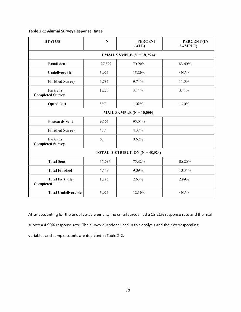
38

Table 2-1: Alumni Survey Response Rates

STATUS N PERCENT (ALL)

PERCENT (IN SAMPLE)

EMAIL SAMPLE (N = 38, 924)

Email Sent 27,592 70.90% 83.60%

Undeliverable 5,921 15.20% <NA>

Finished Survey 3,791 9.74% 11.5%

Partially Completed Survey

1,223 3.14% 3.71%

Opted Out 397 1.02% 1.20%

MAIL SAMPLE (N = 10,000)

Postcards Sent 9,501 95.01%

Finished Survey 437 4.37%

Partially Completed Survey

62 0.62%

TOTAL DISTRIBUTION (N = 48,924)

Total Sent 37,093 75.82% 86.26%

Total Finished 4,448 9.09% 10.34%

Total Partially Completed

1,285 2.63% 2.99%

Total Undeliverable 5,921 12.10% <NA>

After accounting for the undeliverable emails, the email survey had a 15.21% response rate and the mail

survey a 4.99% response rate. The survey questions used in this analysis and their corresponding

variables and sample counts are depicted in Table 2-2.

39

Table 2-2: Survey Questions Used in Study

Question Variable

What year did you graduate from the University of Maine with your {{Most Recent}} Degree?

nyear = 2019 - [Year of Graduation]

Which of the following best describes your marital status?

Married - dummy variable with answers 1 - 2 as Yes and 3-5 as No.

What is the highest level of education you have completed at any university including the University of Maine?

HighEd

Which of the following best describes your major for your {{Most Recent Degree}} from the University of Maine?

University of Maine college grouping School

What was your total personal income, before taxes, in 2018? >What percentage of your personal income was wage income?

Log(income * percent wage) = ln(wage)

If you currently reside in the United States, what is the zip code of your permanent residence?

Zipcode of residence used to optain values for lnCountyPop Unemp_College_P, NAICS.LQ, and SOC.LQ

Which of the following industries most closely matches the industry of your primary employer?

2-dig NAICS code Industry dummy NAICS. LQ

Please tell us what occupation best matches your current job title. Major SOC code Occupation dummy SOC.LQ

How important to you were the following characteristics when choosing to live {{in/outside}} Maine? (1 Not Important) – (6 Extremely Important)/ NA

➢ Career opportunities ➢ Spouse/partner

Dummies to control for location preference Spouse Career

Does your current job require a college degree? DegMatch

Is your current job related to your major field of study at the University of Maine?

majMatch

Additional information on demographics and spatial characteristics is merged with the survey

responses. Data on the age and gender of survey respondents is obtained from the University of Maine

Alumni Association database by matching respondents to their demographic information using their

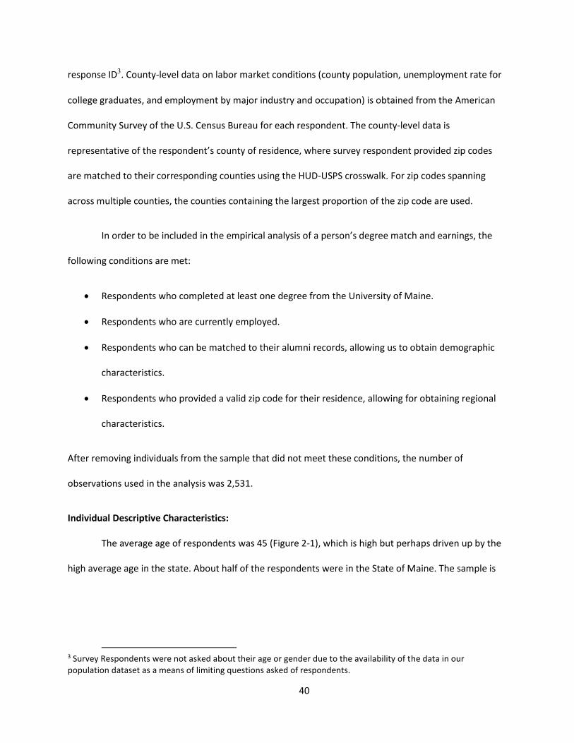
40

response ID3. County-level data on labor market conditions (county population, unemployment rate for

college graduates, and employment by major industry and occupation) is obtained from the American

Community Survey of the U.S. Census Bureau for each respondent. The county-level data is

representative of the respondent’s county of residence, where survey respondent provided zip codes

are matched to their corresponding counties using the HUD-USPS crosswalk. For zip codes spanning

across multiple counties, the counties containing the largest proportion of the zip code are used.

In order to be included in the empirical analysis of a person’s degree match and earnings, the

following conditions are met:

• Respondents who completed at least one degree from the University of Maine.

• Respondents who are currently employed.

• Respondents who can be matched to their alumni records, allowing us to obtain demographic

characteristics.

• Respondents who provided a valid zip code for their residence, allowing for obtaining regional

characteristics.

After removing individuals from the sample that did not meet these conditions, the number of

observations used in the analysis was 2,531.

Individual Descriptive Characteristics:

The average age of respondents was 45 (Figure 2-1), which is high but perhaps driven up by the

high average age in the state. About half of the respondents were in the State of Maine. The sample is

3 Survey Respondents were not asked about their age or gender due to the availability of the data in our population dataset as a means of limiting questions asked of respondents.

41

largely homogeneous in terms of race, with 85% of the respondents having specified that they are

white4.

Figure 2-1: Survey Respondent Age

Over 54% of survey respondents are married on their first marriage and 22.8% have never been

married. The household income for 42.2% of respondents was over $100,000, with 24% at $100,000 to

$149,000. The median individual income was $75,000, with an average of $107,000 driven up by 5

respondents who reported annual incomes of over a million. The average wages calculated by

multiplying the income of the respondents by the percentage of income reported to be from wages,

were $88,398 with a median of $68,000.

For 72% of respondents, the highest achieved degree level was equivalent to their most recent

University of Maine degree, with the proportion of those who received their highest degree level

elsewhere increasing with level of education: 99% of bachelor’s degree holders and only 42% of

4 The National Center for Education Statistics reported that 91% of fall enrollment in Maine in postsecondary institutions in 2008 was by those of the white ethnicity ().

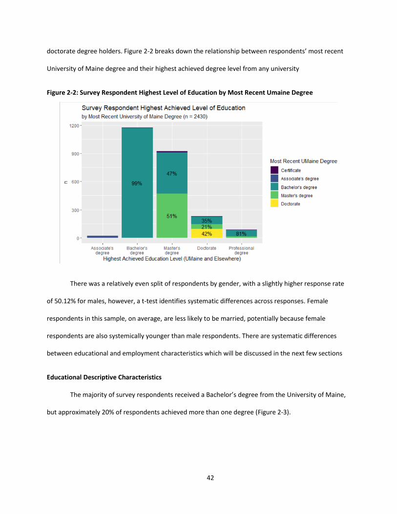
42

doctorate degree holders. Figure 2-2 breaks down the relationship between respondents’ most recent

University of Maine degree and their highest achieved degree level from any university

Figure 2-2: Survey Respondent Highest Level of Education by Most Recent Umaine Degree

There was a relatively even split of respondents by gender, with a slightly higher response rate

of 50.12% for males, however, a t-test identifies systematic differences across responses. Female

respondents in this sample, on average, are less likely to be married, potentially because female

respondents are also systemically younger than male respondents. There are systematic differences

between educational and employment characteristics which will be discussed in the next few sections

Educational Descriptive Characteristics

The majority of survey respondents received a Bachelor’s degree from the University of Maine,

but approximately 20% of respondents achieved more than one degree (Figure 2-3).

43

Figure 2-3: Respondent University of Maine Degree Obtained

An examination of the most recent graduation year (Figure 2-4) shows the response data is skewed with

more respondents from the 2015-2020 graduation decades.

Figure 2-4: Survey Respondent Degree and Graduation Date

The top 5 majors for each of the five UMaine Colleges from the respondent’s most recent

University of Maine degree are shown in Table 2-3. The most common majors of graduates across all

schools were Business Administration, Education, and Civil Engineering. About 8% of survey respondents

achieved degrees with more than one major, the majority of which were combined within a single

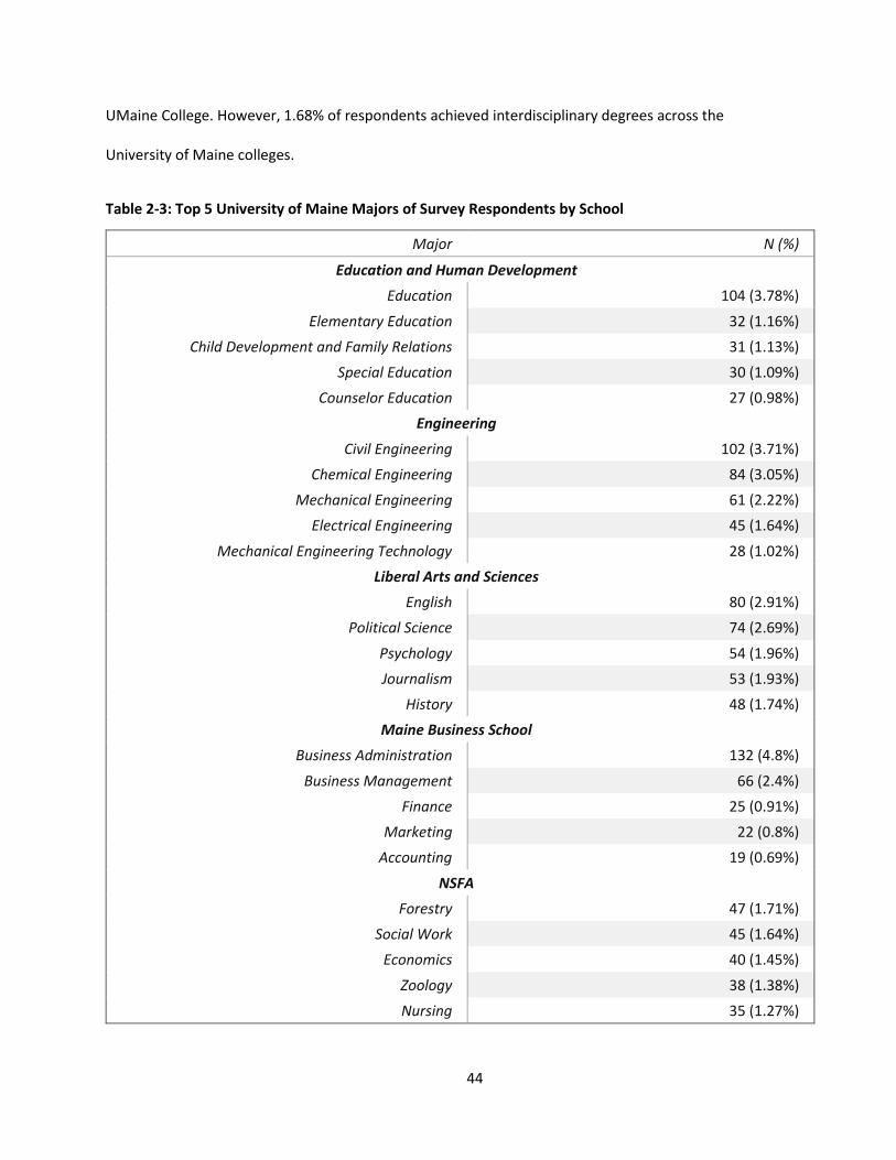
44

UMaine College. However, 1.68% of respondents achieved interdisciplinary degrees across the

University of Maine colleges.

Table 2-3: Top 5 University of Maine Majors of Survey Respondents by School

Major N (%)

Education and Human Development Education 104 (3.78%)

Elementary Education 32 (1.16%) Child Development and Family Relations 31 (1.13%)

Special Education 30 (1.09%) Counselor Education 27 (0.98%)

Engineering Civil Engineering 102 (3.71%)

Chemical Engineering 84 (3.05%) Mechanical Engineering 61 (2.22%)

Electrical Engineering 45 (1.64%) Mechanical Engineering Technology 28 (1.02%)

Liberal Arts and Sciences English 80 (2.91%)

Political Science 74 (2.69%) Psychology 54 (1.96%) Journalism 53 (1.93%)

History 48 (1.74%) Maine Business School

Business Administration 132 (4.8%) Business Management 66 (2.4%)

Finance 25 (0.91%) Marketing 22 (0.8%)

Accounting 19 (0.69%) NSFA

Forestry 47 (1.71%) Social Work 45 (1.64%)

Economics 40 (1.45%) Zoology 38 (1.38%) Nursing 35 (1.27%)

45

There are systematic differences between genders of respondents and the college of the most

recent major (Figure 2-5). The colleges of Education and Human Development, Liberal Arts and Sciences,

and NSFA are largely female dominated, while Engineering and the Maine Business School were largely

male dominated. Furthermore, female respondents, on average, achieve a higher level of educational

attainment and have fewer years since most recent degree.

Figure 2-5: Survey Respondent University of Maine College by Gender

Employment Descriptive Characteristics:

The most common occupation major occupational group was management occupations, with

28% of respondents, followed educational instruction and library occupations at 16% of respondents.

The most common major industry was Educational Services, at 27%, followed by Professional, Scientific,

and Technical Services at 17%. There are systematic differences by gender across major industry and

unequal distributions across both occupation and industry (Figure 2-6).

46

Figure 2-6: Gender Breakdown of major industry and occupation5

The majority of respondents are employed in the private sector, with 70% of respondents

employed in the private sector working for for-profit companies. 32% of respondents are employed in

the public sector. There is a statistically significant difference across genders in employment type. A

larger proportion of women are employed in the public sector by non-profit companies in the public

sector (Figure 2-7).

5 Due to the high heterogeneity across occupations for the sample size, the industries are further grouped in a manner adapted from the Census Occupational major groupings.

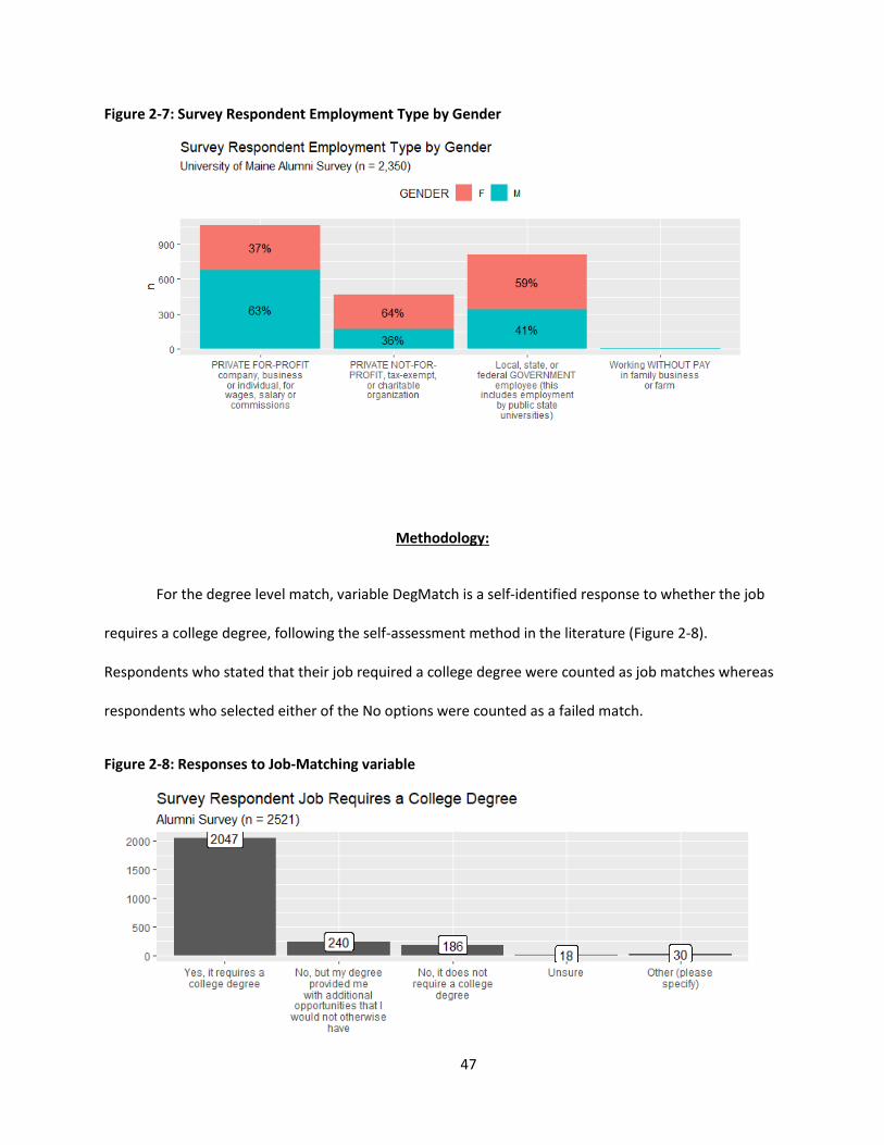
47

Figure 2-7: Survey Respondent Employment Type by Gender

Methodology:

For the degree level match, variable DegMatch is a self-identified response to whether the job

requires a college degree, following the self-assessment method in the literature (Figure 2-8).

Respondents who stated that their job required a college degree were counted as job matches whereas

respondents who selected either of the No options were counted as a failed match.

Figure 2-8: Responses to Job-Matching variable

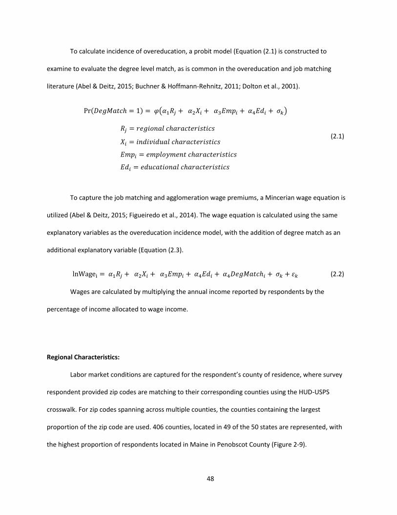
48

To calculate incidence of overeducation, a probit model (Equation (2.1) is constructed to

examine to evaluate the degree level match, as is common in the overeducation and job matching

literature (Abel & Deitz, 2015; Buchner & Hoffmann-Rehnitz, 2011; Dolton et al., 2001).

Pr(𝐷𝑒𝑔𝑀𝑎𝑡𝑐ℎ = 1) = 𝜑(𝛼1𝑅𝑗 + 𝛼2𝑋𝑖 + 𝛼3𝐸𝑚𝑝𝑖 + 𝛼4𝐸𝑑𝑖 + 𝜎𝑘)

𝑅𝑗 = 𝑟𝑒𝑔𝑖𝑜𝑛𝑎𝑙 𝑐ℎ𝑎𝑟𝑎𝑐𝑡𝑒𝑟𝑖𝑠𝑡𝑖𝑐𝑠

𝑋𝑖 = 𝑖𝑛𝑑𝑖𝑣𝑖𝑑𝑢𝑎𝑙 𝑐ℎ𝑎𝑟𝑎𝑐𝑡𝑒𝑟𝑖𝑠𝑡𝑖𝑐𝑠

𝐸𝑚𝑝𝑖 = 𝑒𝑚𝑝𝑙𝑜𝑦𝑚𝑒𝑛𝑡 𝑐ℎ𝑎𝑟𝑎𝑐𝑡𝑒𝑟𝑖𝑠𝑡𝑖𝑐𝑠

𝐸𝑑𝑖 = 𝑒𝑑𝑢𝑐𝑎𝑡𝑖𝑜𝑛𝑎𝑙 𝑐ℎ𝑎𝑟𝑎𝑐𝑡𝑒𝑟𝑖𝑠𝑡𝑖𝑐𝑠

(2.1)

To capture the job matching and agglomeration wage premiums, a Mincerian wage equation is

utilized (Abel & Deitz, 2015; Figueiredo et al., 2014). The wage equation is calculated using the same

explanatory variables as the overeducation incidence model, with the addition of degree match as an

additional explanatory variable (Equation (2.3).

lnWagei = 𝛼1𝑅𝑗 + 𝛼2𝑋𝑖 + 𝛼3𝐸𝑚𝑝𝑖 + 𝛼4𝐸𝑑𝑖 + 𝛼4𝐷𝑒𝑔𝑀𝑎𝑡𝑐ℎ𝑖 + 𝜎𝑘 + 𝜀𝑘 (2.2)

Wages are calculated by multiplying the annual income reported by respondents by the

percentage of income allocated to wage income.

Regional Characteristics:

Labor market conditions are captured for the respondent’s county of residence, where survey

respondent provided zip codes are matching to their corresponding counties using the HUD-USPS

crosswalk. For zip codes spanning across multiple counties, the counties containing the largest

proportion of the zip code are used. 406 counties, located in 49 of the 50 states are represented, with

the highest proportion of respondents located in Maine in Penobscot County (Figure 2-9).

49

Figure 2-9: Alumni Survey Respondents by County of Residence

The unemployment rate of college-graduates or higher (unemp_college_p) is used as a proxy for

job availability (Abel & Deitz, 2015; Büchel & van Ham, 2003). The natural log of population

(lnCountyPop) of the individual’s county of residence is used as a measure for regional urbanization

(Abel & Deitz, 2015; Figueiredo et al., 2014). County size ranges vastly, with the majority of counties

sized less than 2500 (Figure 2-10).

Figure 2-10: Alumni Survey Respondent County of Residence Urbanization

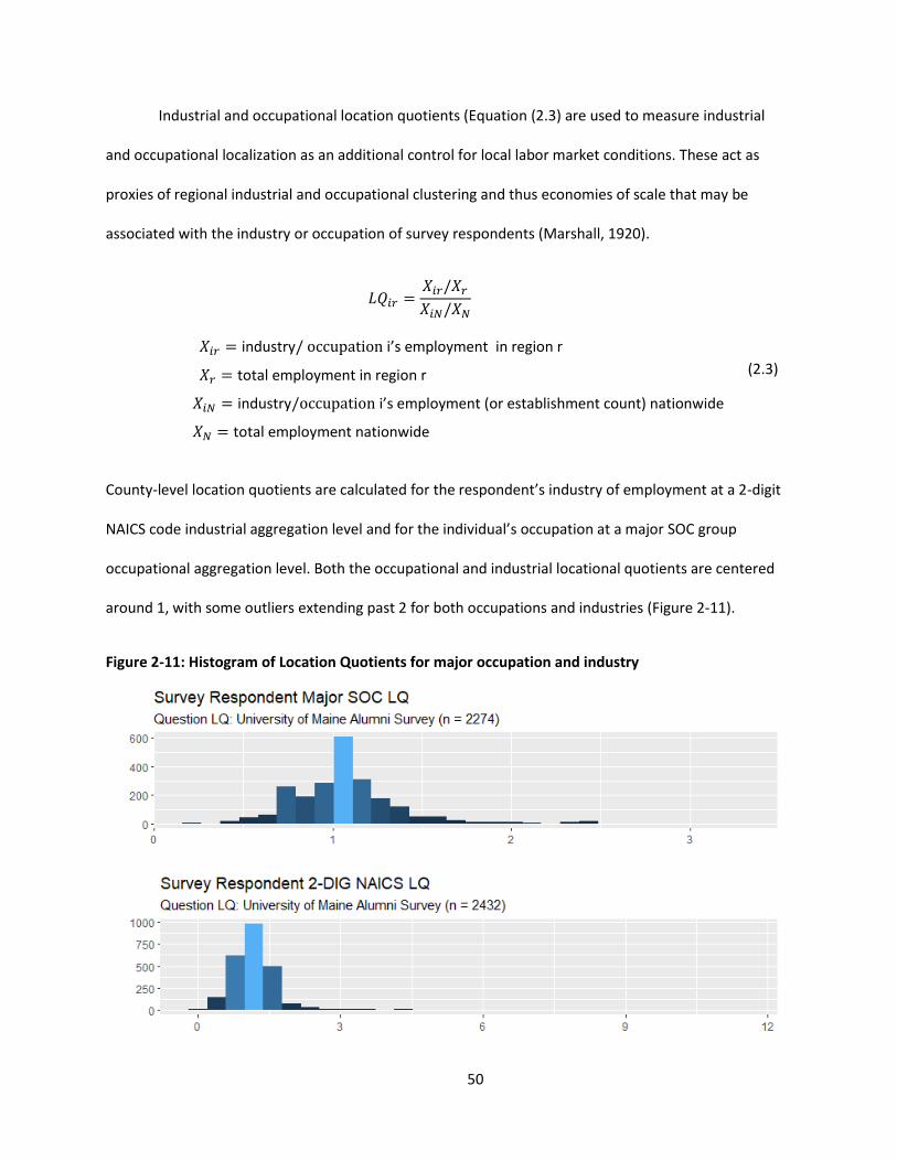
50

Industrial and occupational location quotients (Equation (2.3) are used to measure industrial

and occupational localization as an additional control for local labor market conditions. These act as

proxies of regional industrial and occupational clustering and thus economies of scale that may be

associated with the industry or occupation of survey respondents (Marshall, 1920).

𝐿𝑄𝑖𝑟 =𝑋𝑖𝑟/𝑋𝑟

𝑋𝑖𝑁/𝑋𝑁

𝑋𝑖𝑟 = industry/ occupation i’s employment in region r

𝑋𝑟 = total employment in region r

𝑋𝑖𝑁 = industry/occupation i’s employment (or establishment count) nationwide

𝑋𝑁 = total employment nationwide

(2.3)

County-level location quotients are calculated for the respondent’s industry of employment at a 2-digit

NAICS code industrial aggregation level and for the individual’s occupation at a major SOC group

occupational aggregation level. Both the occupational and industrial locational quotients are centered

around 1, with some outliers extending past 2 for both occupations and industries (Figure 2-11).

Figure 2-11: Histogram of Location Quotients for major occupation and industry

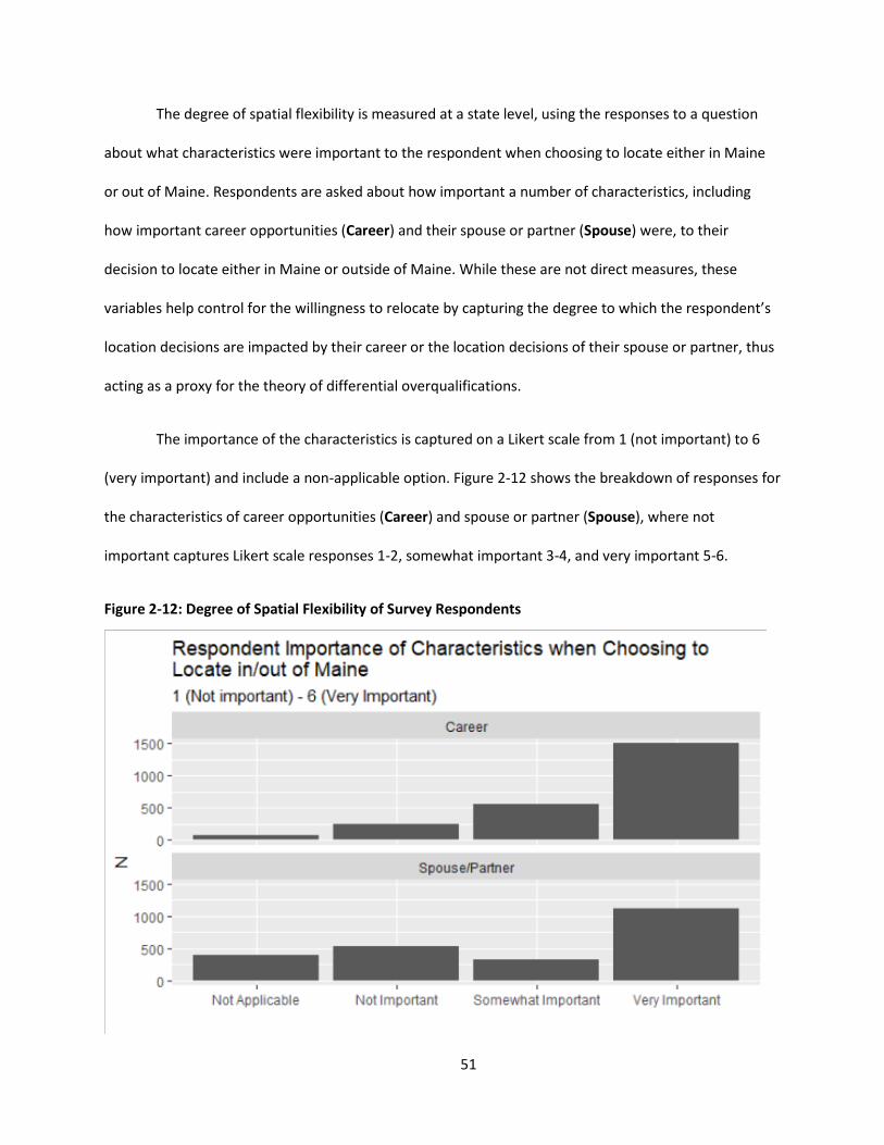
51

The degree of spatial flexibility is measured at a state level, using the responses to a question

about what characteristics were important to the respondent when choosing to locate either in Maine

or out of Maine. Respondents are asked about how important a number of characteristics, including

how important career opportunities (Career) and their spouse or partner (Spouse) were, to their

decision to locate either in Maine or outside of Maine. While these are not direct measures, these

variables help control for the willingness to relocate by capturing the degree to which the respondent’s

location decisions are impacted by their career or the location decisions of their spouse or partner, thus

acting as a proxy for the theory of differential overqualifications.

The importance of the characteristics is captured on a Likert scale from 1 (not important) to 6

(very important) and include a non-applicable option. Figure 2-12 shows the breakdown of responses for

the characteristics of career opportunities (Career) and spouse or partner (Spouse), where not

important captures Likert scale responses 1-2, somewhat important 3-4, and very important 5-6.

Figure 2-12: Degree of Spatial Flexibility of Survey Respondents

52

For simplicity, the variables Career and Spouse are converted into dummy variables for whether the

characteristic was important (Somewhat Important and Very Important groups) or not important (Not

Important and Not Applicable groups)

Employment Characteristics Controls

To control for heterogeneity across industry and occupation of employment, aggregated dummy

variables for the employment descriptive variables are included. Occupations are aggregated at a major

occupational level then further grouped based on Census Occupational groupings. Industry of

employment is reported at a 2-digit NAICS code level and aggregated based on Census major industrial

groupings. To further preserve explanatory power, occupations and industries with less than 75

responses are grouped into an “other” category.

Educational Characteristic Controls

Number of years since obtaining the most recent University of Maine degree (nyears) is used as

a proxy for years of experience, showing time since respondents achieved their most recent University

of Maine degree. Highest degree attained by the respondent (HighEd) is used in place of degree level

from the University of Maine degree to cover due to skillset from the additional degree gained.

To account for differences in educational characteristics of respondents, the majors of the

respondents most recent degree are grouped into their respective college at the University of Maine

(College).

Individual Characteristic Controls:

The model controls for commonly used demographic characteristics: namely gender of

respondent and marital status (married). Respondents race is not included due to the data’s

homogenous nature, with 86% of the respondents specifying that they are white. Number of kids, while

shown to be significant towards determining job match, was not important by AIC/BIC criteria and was

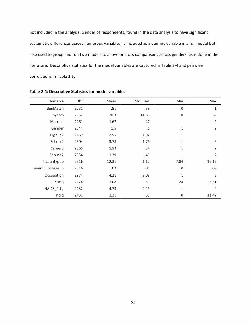
53

not included in the analysis. Gender of respondents, found in the data analysis to have significant

systematic differences across numerous variables, is included as a dummy variable in a full model but

also used to group and run two models to allow for cross comparisons across genders, as is done in the

literature. Descriptive statistics for the model variables are captured in Table 2-4 and pairwise

correlations in Table 2-5.

Table 2-4: Descriptive Statistics for model variables

Variable Obs Mean Std. Dev. Min Max

degMatch 2531 .81 .39 0 1

nyears 2552 20.3 14.63 0 62

Married 2461 1.67 .47 1 2

Gender 2544 1.5 .5 1 2

HighEd2 2469 2.95 1.02 1 5

School2 2504 3.78 1.79 1 6

Career3 2365 1.13 .34 1 2

Spouse2 2354 1.39 .49 1 2

lncountypop 2516 12.31 1.12 7.84 16.12

unemp_college_p 2516 .02 .01 0 .08

Occupation 2274 4.21 2.08 1 8

soclq 2274 1.08 .31 .24 3.31

NAICS_2dig 2432 4.73 2.49 1 9

indlq 2432 1.21 .65 0 11.42

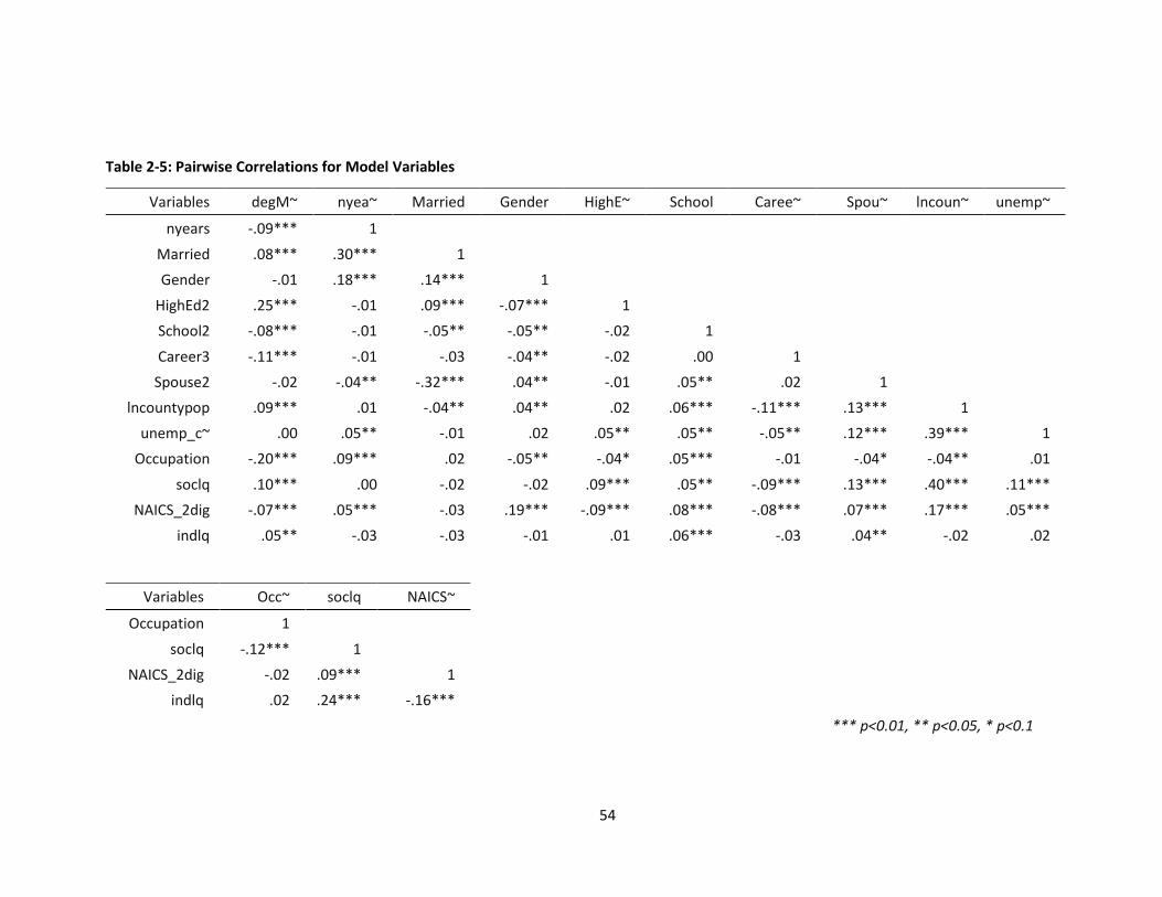
54

Table 2-5: Pairwise Correlations for Model Variables

Variables degM~ nyea~ Married Gender HighE~ School Caree~ Spou~ lncoun~ unemp~

nyears -.09*** 1 Married .08*** .30*** 1 Gender -.01 .18*** .14*** 1

HighEd2 .25*** -.01 .09*** -.07*** 1 School2 -.08*** -.01 -.05** -.05** -.02 1 Career3 -.11*** -.01 -.03 -.04** -.02 .00 1

Spouse2 -.02 -.04** -.32*** .04** -.01 .05** .02 1 lncountypop .09*** .01 -.04** .04** .02 .06*** -.11*** .13*** 1

unemp_c~ .00 .05** -.01 .02 .05** .05** -.05** .12*** .39*** 1 Occupation -.20*** .09*** .02 -.05** -.04* .05*** -.01 -.04* -.04** .01

soclq .10*** .00 -.02 -.02 .09*** .05** -.09*** .13*** .40*** .11*** NAICS_2dig -.07*** .05*** -.03 .19*** -.09*** .08*** -.08*** .07*** .17*** .05***

indlq .05** -.03 -.03 -.01 .01 .06*** -.03 .04** -.02 .02

Variables Occ~ soclq NAICS~

Occupation 1 soclq -.12*** 1

NAICS_2dig -.02 .09*** 1 indlq .02 .24*** -.16***

*** p<0.01, ** p<0.05, * p<0.1

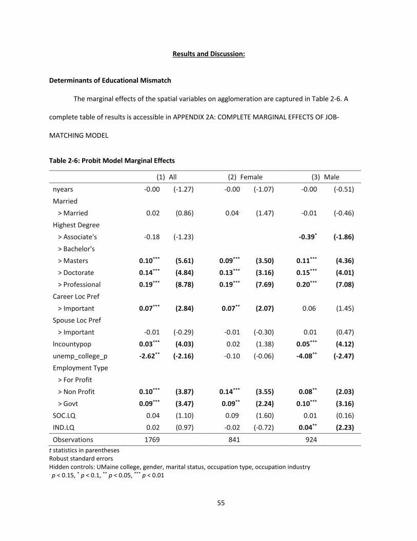
55

Results and Discussion:

Determinants of Educational Mismatch

The marginal effects of the spatial variables on agglomeration are captured in Table 2-6. A

complete table of results is accessible in APPENDIX 2A: COMPLETE MARGINAL EFFECTS OF JOB-

MATCHING MODEL

Table 2-6: Probit Model Marginal Effects

(1) All (2) Female (3) Male

nyears -0.00 (-1.27) -0.00 (-1.07) -0.00 (-0.51) Married > Married 0.02 (0.86) 0.04. (1.47) -0.01 (-0.46) Highest Degree > Associate's -0.18 (-1.23) -0.39* (-1.86) > Bachelor's > Masters 0.10*** (5.61) 0.09*** (3.50) 0.11*** (4.36) > Doctorate 0.14*** (4.84) 0.13*** (3.16) 0.15*** (4.01) > Professional 0.19*** (8.78) 0.19*** (7.69) 0.20*** (7.08) Career Loc Pref > Important 0.07*** (2.84) 0.07** (2.07) 0.06. (1.45) Spouse Loc Pref > Important -0.01 (-0.29) -0.01 (-0.30) 0.01 (0.47) lncountypop 0.03*** (4.03) 0.02 (1.38) 0.05*** (4.12) unemp_college_p -2.62** (-2.16) -0.10 (-0.06) -4.08** (-2.47) Employment Type > For Profit > Non Profit 0.10*** (3.87) 0.14*** (3.55) 0.08** (2.03) > Govt 0.09*** (3.47) 0.09** (2.24) 0.10*** (3.16) SOC.LQ 0.04 (1.10) 0.09. (1.60) 0.01 (0.16) IND.LQ 0.02 (0.97) -0.02 (-0.72) 0.04** (2.23)

Observations 1769 841 924 t statistics in parentheses Robust standard errors Hidden controls: UMaine college, gender, marital status, occupation type, occupation industry . p < 0.15, * p < 0.1, ** p < 0.05, *** p < 0.01

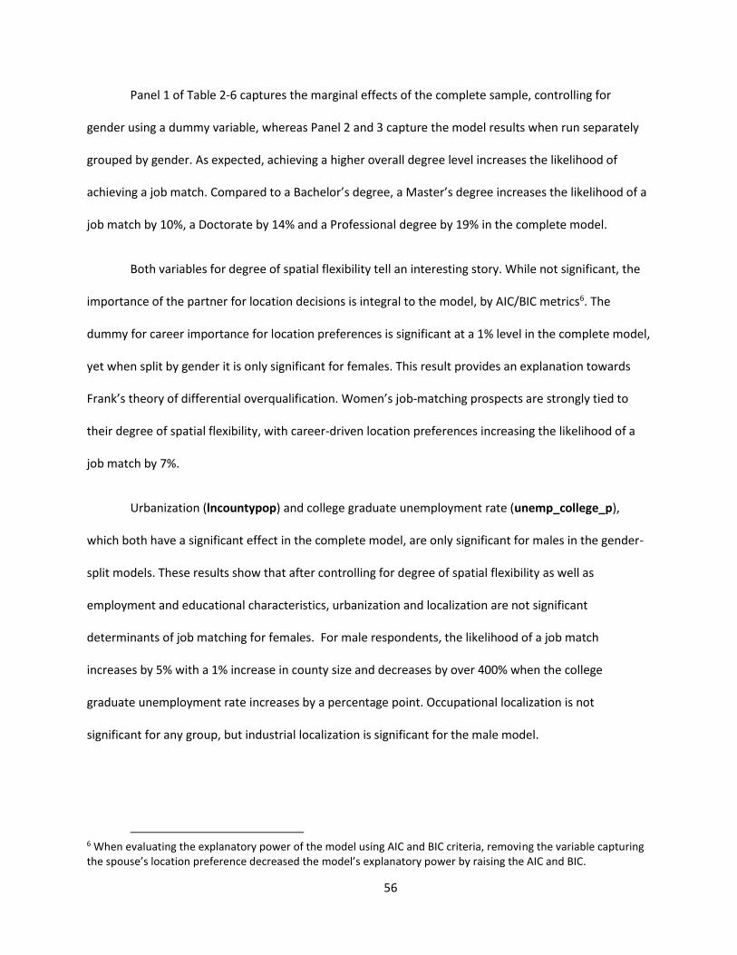
56

Panel 1 of Table 2-6 captures the marginal effects of the complete sample, controlling for

gender using a dummy variable, whereas Panel 2 and 3 capture the model results when run separately

grouped by gender. As expected, achieving a higher overall degree level increases the likelihood of

achieving a job match. Compared to a Bachelor’s degree, a Master’s degree increases the likelihood of a

job match by 10%, a Doctorate by 14% and a Professional degree by 19% in the complete model.

Both variables for degree of spatial flexibility tell an interesting story. While not significant, the

importance of the partner for location decisions is integral to the model, by AIC/BIC metrics6. The

dummy for career importance for location preferences is significant at a 1% level in the complete model,

yet when split by gender it is only significant for females. This result provides an explanation towards

Frank’s theory of differential overqualification. Women’s job-matching prospects are strongly tied to

their degree of spatial flexibility, with career-driven location preferences increasing the likelihood of a

job match by 7%.

Urbanization (lncountypop) and college graduate unemployment rate (unemp_college_p),

which both have a significant effect in the complete model, are only significant for males in the gender-

split models. These results show that after controlling for degree of spatial flexibility as well as

employment and educational characteristics, urbanization and localization are not significant

determinants of job matching for females. For male respondents, the likelihood of a job match

increases by 5% with a 1% increase in county size and decreases by over 400% when the college

graduate unemployment rate increases by a percentage point. Occupational localization is not

significant for any group, but industrial localization is significant for the male model.

6 When evaluating the explanatory power of the model using AIC and BIC criteria, removing the variable capturing the spouse’s location preference decreased the model’s explanatory power by raising the AIC and BIC.

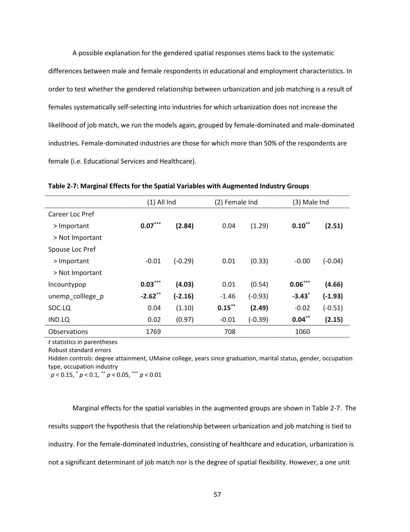
57

A possible explanation for the gendered spatial responses stems back to the systematic

differences between male and female respondents in educational and employment characteristics. In

order to test whether the gendered relationship between urbanization and job matching is a result of

females systematically self-selecting into industries for which urbanization does not increase the

likelihood of job match, we run the models again, grouped by female-dominated and male-dominated

industries. Female-dominated industries are those for which more than 50% of the respondents are

female (i.e. Educational Services and Healthcare).

Table 2-7: Marginal Effects for the Spatial Variables with Augmented Industry Groups

(1) All Ind (2) Female Ind (3) Male Ind

Career Loc Pref > Important 0.07*** (2.84) 0.04 (1.29) 0.10** (2.51) > Not Important Spouse Loc Pref > Important -0.01 (-0.29) 0.01 (0.33) -0.00 (-0.04) > Not Important lncountypop 0.03*** (4.03) 0.01 (0.54) 0.06*** (4.66) unemp_colllege_p -2.62** (-2.16) -1.46 (-0.93) -3.43* (-1.93) SOC.LQ 0.04 (1.10) 0.15** (2.49) -0.02 (-0.51) IND.LQ 0.02 (0.97) -0.01 (-0.39) 0.04** (2.15)

Observations 1769 708 1060 t statistics in parentheses Robust standard errors Hidden controls: degree attainment, UMaine college, years since graduation, marital status, gender, occupation type, occupation industry . p < 0.15, * p < 0.1, ** p < 0.05, *** p < 0.01

Marginal effects for the spatial variables in the augmented groups are shown in Table 2-7. The

results support the hypothesis that the relationship between urbanization and job matching is tied to

industry. For the female-dominated industries, consisting of healthcare and education, urbanization is

not a significant determinant of job match nor is the degree of spatial flexibility. However, a one unit

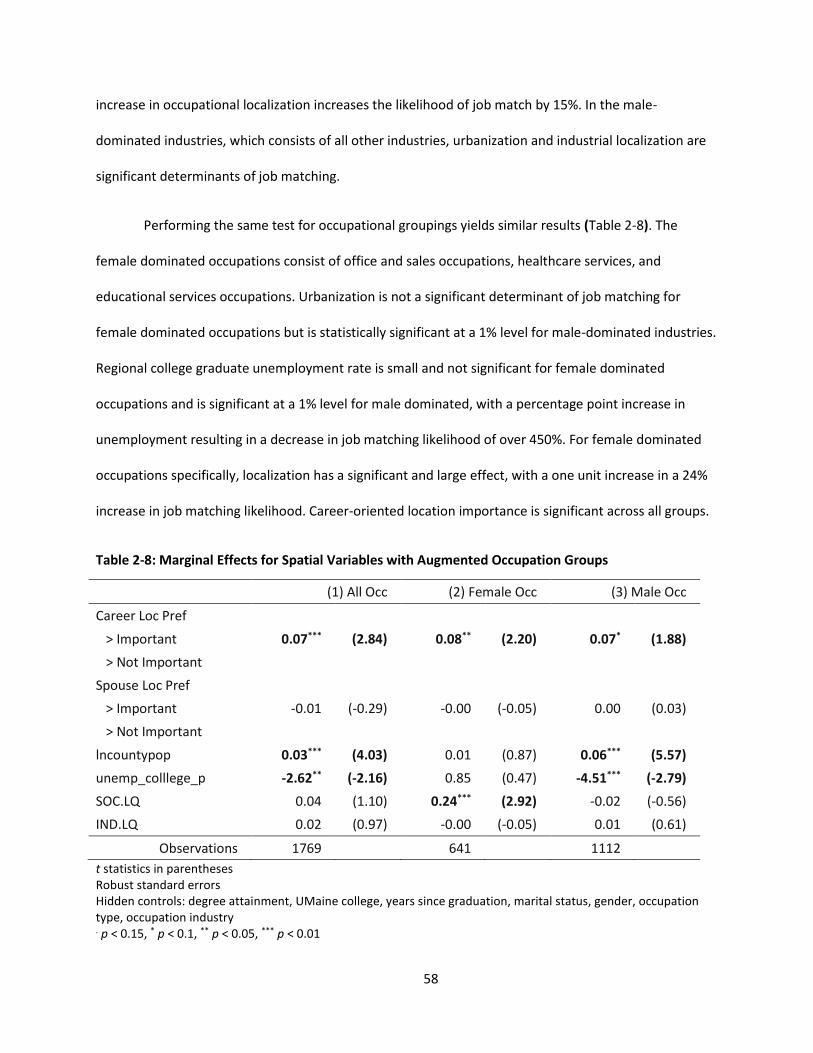
58

increase in occupational localization increases the likelihood of job match by 15%. In the male-

dominated industries, which consists of all other industries, urbanization and industrial localization are

significant determinants of job matching.

Performing the same test for occupational groupings yields similar results (Table 2-8). The

female dominated occupations consist of office and sales occupations, healthcare services, and

educational services occupations. Urbanization is not a significant determinant of job matching for

female dominated occupations but is statistically significant at a 1% level for male-dominated industries.

Regional college graduate unemployment rate is small and not significant for female dominated

occupations and is significant at a 1% level for male dominated, with a percentage point increase in

unemployment resulting in a decrease in job matching likelihood of over 450%. For female dominated

occupations specifically, localization has a significant and large effect, with a one unit increase in a 24%

increase in job matching likelihood. Career-oriented location importance is significant across all groups.

Table 2-8: Marginal Effects for Spatial Variables with Augmented Occupation Groups

(1) All Occ (2) Female Occ (3) Male Occ

Career Loc Pref > Important 0.07*** (2.84) 0.08** (2.20) 0.07* (1.88) > Not Important Spouse Loc Pref > Important -0.01 (-0.29) -0.00 (-0.05) 0.00 (0.03) > Not Important lncountypop 0.03*** (4.03) 0.01 (0.87) 0.06*** (5.57) unemp_colllege_p -2.62** (-2.16) 0.85 (0.47) -4.51*** (-2.79) SOC.LQ 0.04 (1.10) 0.24*** (2.92) -0.02 (-0.56) IND.LQ 0.02 (0.97) -0.00 (-0.05) 0.01 (0.61)

Observations 1769 641 1112 t statistics in parentheses Robust standard errors Hidden controls: degree attainment, UMaine college, years since graduation, marital status, gender, occupation type, occupation industry . p < 0.15, * p < 0.1, ** p < 0.05, *** p < 0.01

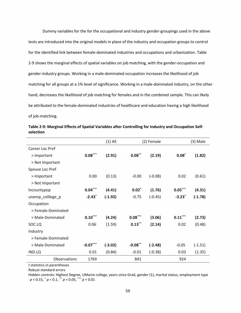
59

Dummy variables for the for the occupational and industry gender-groupings used in the above

tests are introduced into the original models in place of the industry and occupation groups to control

for the identified link between female-dominated industries and occupations and urbanization. Table

2-9 shows the marginal effects of spatial variables on job matching, with the gender-occupation and

gender-industry groups. Working in a male-dominated occupation increases the likelihood of job

matching for all groups at a 1% level of significance. Working in a male-dominated industry, on the other

hand, decreases the likelihood of job matching for females and in the combined sample. This can likely

be attributed to the female-dominated industries of healthcare and education having a high likelihood

of job-matching.

Table 2-9: Marginal Effects of Spatial Variables after Controlling for Industry and Occupation Self-selection

(1) All (2) Female (3) Male

Career Loc Pref > Important 0.08*** (2.91) 0.08** (2.19) 0.08* (1.82) > Not Important Spouse Loc Pref > Important 0.00 (0.13) -0.00 (-0.08) 0.02 (0.61) > Not Important lncountypop 0.04*** (4.41) 0.02* (1.76) 0.05*** (4.31) unemp_colllege_p -2.43* (-1.92) -0.75 (-0.45) -3.23* (-1.78) Occupation > Female-Dominated > Male-Dominated 0.10*** (4.24) 0.08*** (3.06) 0.11*** (2.73) SOC.LQ 0.06. (1.59) 0.13** (2.14) 0.02 (0.48) Industry > Female-Dominated > Male-Dominated -0.07*** (-3.02) -0.08** (-2.48) -0.05. (-1.51) IND.LQ 0.01 (0.84) -0.01 (-0.38) 0.03 (1.35)

Observations 1769 841 924 t statistics in parentheses Robust standard errors Hidden controls: Highest Degree, UMaine college, years since Grad, gender (1), marital status, employment type . p < 0.15, * p < 0.1, ** p < 0.05, *** p < 0.01

60

These results are conducive with the above theory of differences in employment characteristics

for female-dominated and male-dominated industries effecting the link between gender and

urbanization. After controlling for the employment self-selection, urbanization becomes impactful for all

categories. Career location preference is significant for the combined group and both genders.

Occupational localization is significant only for the female group.

Job Match Wage Premium

To understand the wage implications of the college job-match on wages, a Mincerian model is

run, with dependent variable log(wages). Regression results are shown in Table 2-10. For the combined

group as well as each gendered model, degree match has a significant and large impact on wages. A

degree match increases wages by 40%-44%, depending on gender group, ceteris paribus. Urbanization is

significant across all the groups but is largest for females. A 1% increase in county of residence increases

wages by 10% for women, at a 1% level of significance. The model does not identify an effect of spatial

mobility or localization on wages after controlling for individual, educational, employment, and regional

labor market characteristics.

Number of years since school has a positive impact on wages, with a significant yet non-

consequential diminishing effect. These findings are in support of the theory of career mobility. Marital

status has a positive effect on wages across genders, but the effect is the smallest for women. Increases

in degree level also tend to increase wages across all models. Compared to a Bachelor’s degree, a

Masters degree increases wages by 12%, a Doctorate degree by 29%, and a Professional degree by 44%

for the complete model. The female group, compared to the male group, experiences a smaller wage

premium from a masters and professional degree, but a higher premium from a doctorate degree.

61

Table 2-10: Marginal Effects of Degree Match and Spatial Variables on ln(wages).

(1) All (2) Female (3) Male degMatch 0.43*** (5.15) 0.44*** (5.00) 0.40*** (3.03) NYEARS 0.06*** (11.51) 0.07*** (8.53) 0.06*** (8.15) NYEARS # NYEARS -0.00*** (-8.33) -0.00*** (-6.71) -0.00*** (-5.96) Married > Not Married > Married 0.22*** (5.57) 0.14*** (2.64) 0.28*** (4.60) Highest Degree > Associate's -0.55. (-1.49) -0.36 (-1.39) -0.70 (-1.37) > Bachelor's > Masters 0.12*** (2.99) 0.12** (2.38) 0.14** (2.25) > Doctorate 0.29*** (4.89) 0.39*** (3.69) 0.21*** (2.71) > Professional 0.44*** (4.02) 0.35*** (2.67) 0.57*** (3.61) Career Loc Pref > Important 0.03 (0.55) 0.08 (1.19) -0.05 (-0.61) > Not Important Spouse Loc Pref > Important 0.00 (0.10) 0.05 (0.98) -0.01 (-0.10) > Not Important lncountypop 0.08*** (4.29) 0.10*** (3.78) 0.06** (2.49) UNEMP_COLLEGE_P 1.93 (0.70) 3.00 (0.81) 1.91 (0.42) Employment Type > For Profit > Non Profit -0.14** (-2.38) -0.05 (-0.47) -0.22*** (-3.36) > Govt -0.10. (-1.54) 0.02 (0.29) -0.23** (-2.41) SOC.LQ 0.09. (1.53) 0.00 (0.00) 0.14. (1.60) IND.LQ 0.03 (1.09) 0.05 (1.16) 0.03 (0.84) Constant 8.45*** (37.28) 7.95*** (23.38) 8.56*** (27.54) Observations 1588 754 834

t statistics in parentheses Robust standard errors Hidden controls: UMaine college, gender. occupation, occupation industry . p < 0.15, * p < 0.1, ** p < 0.05, *** p < 0.01

Compared to employment in the for-profit sector, employment in the non-profit sector

decreases wages by approximately 14% for the complete model and by 22% in the male-only model.

Being employed in the public sector decreases wages by 23% in the male-only model. No effect is

identified in the female model, perhaps due to the fact that there is a link between job matches and

employment type and the majority of women are employed in either the non-profit or public sector

jobs.

62

Limitations:

The dataset used in this study is limited in size and scope to only University of Maine graduates

and, therefore, caution must be used when applying conclusions from this research as applicable to the

general US population and general college graduate population. The small size of the sample did not

allow for regional fixed effects to be included in the model, thus limiting the explanatory power of this

model. Furthermore, survey respondents were spatially concentrated in Maine.

Another limiting factor is that the data is cross-sectional and does not have information about

the respondents over time. Furthermore, the respondents are asked only about their most recent job,

not their first job over college. This is done to reduce the number of questions asked of respondents but

significantly limits the research scope because it decreases the useable sample size considerably. Self-

employed and retired employees were not asked about overeducation to limit question fatigue, thus

further limiting the sample size by 33%.

While significant and interesting, the variables used to proxy degree of spatial flexibility are

limited in their explanatory power. More preferable metrics of degree of spatial flexibility include

commuting distance, commuting ability, etc. Furthermore, no information is collected on the firm

characteristics or reasons for accepting the job, also drivers of overeducation models.

Conclusion:

This paper investigated the effect of regional agglomeration on job matching for University of

Maine graduates. The findings in this paper confirm the theory that regional agglomeration is significant

in labor-market matching. Interestingly, the findings show that effect of regional agglomeration is highly

impacted not only by gender of respondents but by the unequal self-selection of respondents into

occupational and industry groupings.

63

Occupational localization is significant for female-dominated industries (i.e. educational

services, and healthcare and social assistance) and female-dominated occupations (educational

instruction and library occupations, healthcare practitioners and technical occupations, and sales and

office occupations). Industrial localization is significant for male-dominated industries only. After

controlling for the industrial specialization urbanization, a significant determinant of job matching for

male dominated industries and occupations, is shown to be a determinant for both genders and

occupational localization for both females and males. As found in previous literature (Abel & Deitz,

2015; Figueiredo et al., 2014; Freeman, 1976) there is a wage premium associated with job matching

and urbanization but the paper does not find a localization wage premium.

With US college debt levels at $1.47 trillion in 2018, understanding the determinants and

implications of overeducation is not just interesting; it is critical. College graduates are faced with

decisions on where to locate after graduation and awareness of the implications of that decision on

their likelihood of overeducation and their expected wages could be beneficial to their long run success.

Furthermore, the differences in these implications by gender and gender-industry relationship cannot

be ignored.

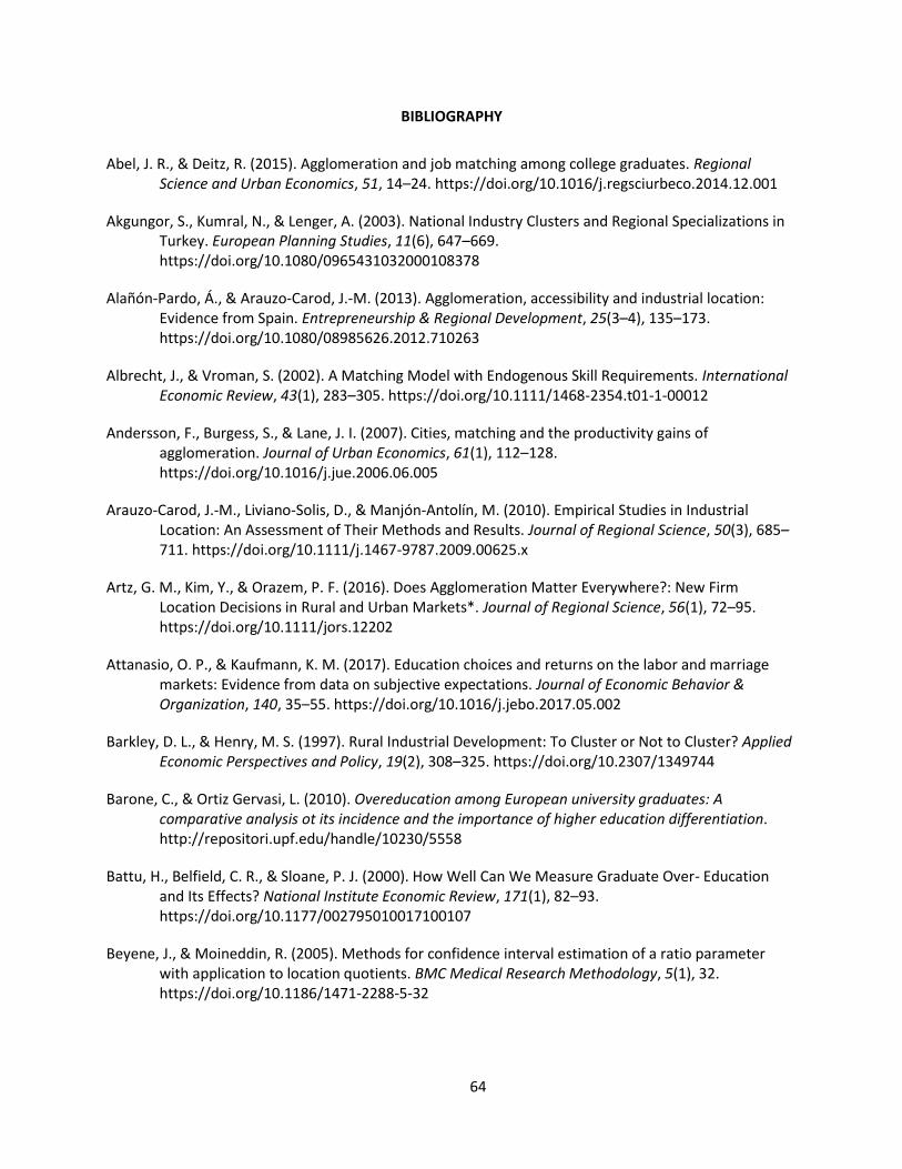
64

BIBLIOGRAPHY

Abel, J. R., & Deitz, R. (2015). Agglomeration and job matching among college graduates. Regional Science and Urban Economics, 51, 14–24. https://doi.org/10.1016/j.regsciurbeco.2014.12.001

Akgungor, S., Kumral, N., & Lenger, A. (2003). National Industry Clusters and Regional Specializations in Turkey. European Planning Studies, 11(6), 647–669. https://doi.org/10.1080/0965431032000108378

Alañón-Pardo, Á., & Arauzo-Carod, J.-M. (2013). Agglomeration, accessibility and industrial location: Evidence from Spain. Entrepreneurship & Regional Development, 25(3–4), 135–173. https://doi.org/10.1080/08985626.2012.710263

Albrecht, J., & Vroman, S. (2002). A Matching Model with Endogenous Skill Requirements. International Economic Review, 43(1), 283–305. https://doi.org/10.1111/1468-2354.t01-1-00012

Andersson, F., Burgess, S., & Lane, J. I. (2007). Cities, matching and the productivity gains of agglomeration. Journal of Urban Economics, 61(1), 112–128. https://doi.org/10.1016/j.jue.2006.06.005

Arauzo-Carod, J.-M., Liviano-Solis, D., & Manjón-Antolín, M. (2010). Empirical Studies in Industrial Location: An Assessment of Their Methods and Results. Journal of Regional Science, 50(3), 685–711. https://doi.org/10.1111/j.1467-9787.2009.00625.x

Artz, G. M., Kim, Y., & Orazem, P. F. (2016). Does Agglomeration Matter Everywhere?: New Firm Location Decisions in Rural and Urban Markets*. Journal of Regional Science, 56(1), 72–95. https://doi.org/10.1111/jors.12202

Attanasio, O. P., & Kaufmann, K. M. (2017). Education choices and returns on the labor and marriage markets: Evidence from data on subjective expectations. Journal of Economic Behavior & Organization, 140, 35–55. https://doi.org/10.1016/j.jebo.2017.05.002

Barkley, D. L., & Henry, M. S. (1997). Rural Industrial Development: To Cluster or Not to Cluster? Applied Economic Perspectives and Policy, 19(2), 308–325. https://doi.org/10.2307/1349744

Barone, C., & Ortiz Gervasi, L. (2010). Overeducation among European university graduates: A comparative analysis ot its incidence and the importance of higher education differentiation. http://repositori.upf.edu/handle/10230/5558

Battu, H., Belfield, C. R., & Sloane, P. J. (2000). How Well Can We Measure Graduate Over- Education and Its Effects? National Institute Economic Review, 171(1), 82–93. https://doi.org/10.1177/002795010017100107

Beyene, J., & Moineddin, R. (2005). Methods for confidence interval estimation of a ratio parameter with application to location quotients. BMC Medical Research Methodology, 5(1), 32. https://doi.org/10.1186/1471-2288-5-32

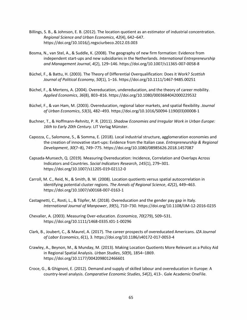
65

Billings, S. B., & Johnson, E. B. (2012). The location quotient as an estimator of industrial concentration. Regional Science and Urban Economics, 42(4), 642–647. https://doi.org/10.1016/j.regsciurbeco.2012.03.003

Bosma, N., van Stel, A., & Suddle, K. (2008). The geography of new firm formation: Evidence from independent start-ups and new subsidiaries in the Netherlands. International Entrepreneurship and Management Journal, 4(2), 129–146. https://doi.org/10.1007/s11365-007-0058-8

Büchel, F., & Battu, H. (2003). The Theory of Differential Overqualification: Does it Work? Scottish Journal of Political Economy, 50(1), 1–16. https://doi.org/10.1111/1467-9485.00251

Büchel, F., & Mertens, A. (2004). Overeducation, undereducation, and the theory of career mobility. Applied Economics, 36(8), 803–816. https://doi.org/10.1080/0003684042000229532

Büchel, F., & van Ham, M. (2003). Overeducation, regional labor markets, and spatial flexibility. Journal of Urban Economics, 53(3), 482–493. https://doi.org/10.1016/S0094-1190(03)00008-1

Buchner, T., & Hoffmann-Rehnitz, P. R. (2011). Shadow Economies and Irregular Work in Urban Europe: 16th to Early 20th Century. LIT Verlag Münster.

Capozza, C., Salomone, S., & Somma, E. (2018). Local industrial structure, agglomeration economies and the creation of innovative start-ups: Evidence from the Italian case. Entrepreneurship & Regional Development, 30(7–8), 749–775. https://doi.org/10.1080/08985626.2018.1457087

Capsada-Munsech, Q. (2019). Measuring Overeducation: Incidence, Correlation and Overlaps Across Indicators and Countries. Social Indicators Research, 145(1), 279–301. https://doi.org/10.1007/s11205-019-02112-0

Carroll, M. C., Reid, N., & Smith, B. W. (2008). Location quotients versus spatial autocorrelation in identifying potential cluster regions. The Annals of Regional Science, 42(2), 449–463. https://doi.org/10.1007/s00168-007-0163-1

Castagnetti, C., Rosti, L., & Töpfer, M. (2018). Overeducation and the gender pay gap in Italy. International Journal of Manpower, 39(5), 710–730. https://doi.org/10.1108/IJM-12-2016-0235

Chevalier, A. (2003). Measuring Over-education. Economica, 70(279), 509–531. https://doi.org/10.1111/1468-0335.t01-1-00296

Clark, B., Joubert, C., & Maurel, A. (2017). The career prospects of overeducated Americans. IZA Journal of Labor Economics, 6(1), 3. https://doi.org/10.1186/s40172-017-0053-4

Crawley, A., Beynon, M., & Munday, M. (2013). Making Location Quotients More Relevant as a Policy Aid in Regional Spatial Analysis. Urban Studies, 50(9), 1854–1869. https://doi.org/10.1177/0042098012466601

Croce, G., & Ghignoni, E. (2012). Demand and supply of skilled labour and overeducation in Europe: A country-level analysis. Comparative Economic Studies, 54(2), 413-. Gale Academic OneFile.

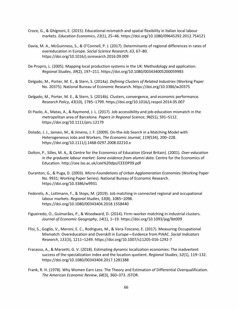
66

Croce, G., & Ghignoni, E. (2015). Educational mismatch and spatial flexibility in Italian local labour markets. Education Economics, 23(1), 25–46. https://doi.org/10.1080/09645292.2012.754121

Davia, M. A., McGuinness, S., & O’Connell, P. J. (2017). Determinants of regional differences in rates of overeducation in Europe. Social Science Research, 63, 67–80. https://doi.org/10.1016/j.ssresearch.2016.09.009

De Propris, L. (2005). Mapping local production systems in the UK: Methodology and application. Regional Studies, 39(2), 197–211. https://doi.org/10.1080/003434005200059983

Delgado, M., Porter, M. E., & Stern, S. (2014a). Defining Clusters of Related Industries (Working Paper No. 20375). National Bureau of Economic Research. https://doi.org/10.3386/w20375

Delgado, M., Porter, M. E., & Stern, S. (2014b). Clusters, convergence, and economic performance. Research Policy, 43(10), 1785–1799. https://doi.org/10.1016/j.respol.2014.05.007

Di Paolo, A., Matas, A., & Raymond, J. L. (2017). Job accessibility and job-education mismatch in the metropolitan area of Barcelona. Papers in Regional Science, 96(S1), S91–S112. https://doi.org/10.1111/pirs.12179

Dolado, J. J., Jansen, M., & Jimeno, J. F. (2009). On‐the‐Job Search in a Matching Model with Heterogeneous Jobs and Workers. The Economic Journal, 119(534), 200–228. https://doi.org/10.1111/j.1468-0297.2008.02210.x

Dolton, P., Silles, M. A., & Centre for the Economics of Education (Great Britain). (2001). Over-education in the graduate labour market: Some evidence from alumni data. Centre for the Economics of Education. http://cee.lse.ac.uk/cee%20dps/CEEDP09.pdf

Duranton, G., & Puga, D. (2003). Micro-Foundations of Urban Agglomeration Economies (Working Paper No. 9931; Working Paper Series). National Bureau of Economic Research. https://doi.org/10.3386/w9931

Fedorets, A., Lottmann, F., & Stops, M. (2019). Job matching in connected regional and occupational labour markets. Regional Studies, 53(8), 1085–1098. https://doi.org/10.1080/00343404.2018.1558440

Figueiredo, O., Guimarães, P., & Woodward, D. (2014). Firm–worker matching in industrial clusters. Journal of Economic Geography, 14(1), 1–19. https://doi.org/10.1093/jeg/lbt009

Flisi, S., Goglio, V., Meroni, E. C., Rodrigues, M., & Vera-Toscano, E. (2017). Measuring Occupational Mismatch: Overeducation and Overskill in Europe—Evidence from PIAAC. Social Indicators Research, 131(3), 1211–1249. https://doi.org/10.1007/s11205-016-1292-7

Fracasso, A., & Marzetti, G. V. (2018). Estimating dynamic localization economies: The inadvertent success of the specialization index and the location quotient. Regional Studies, 52(1), 119–132. https://doi.org/10.1080/00343404.2017.1281388

Frank, R. H. (1978). Why Women Earn Less: The Theory and Estimation of Differential Overqualification. The American Economic Review, 68(3), 360–373. JSTOR.

67

Freeman, R. (1976). The Overeducated American. Academic Press.

Frenken, K., van Oort, F. G., Verburg, T., & Boschma, R. A. (2005). Variety and Regional Economic Growth in the Netherlands (SSRN Scholarly Paper ID 871804). Social Science Research Network. https://doi.org/10.2139/ssrn.871804

Gabe, T. (2003). Local Industry Agglomeration and New Business Activity. Growth and Change, 34(1), 17–39. https://doi.org/10.1111/1468-2257.00197

Gabe, T., & Bell, K. (2004). Tradeoffs between Local Taxes and Government Spending as Determinants of Business Location. Journal of Regional Science, 44(1), 21–41. https://doi.org/10.1111/j.1085-9489.2004.00326.x

Glaeser, E. L., & Gottlieb, J. D. (2009). The Wealth of Cities: Agglomeration Economies and Spatial Equilibrium in the United States. Journal of Economic Literature, 47(4), 983–1028. https://doi.org/10.1257/jel.47.4.983

Groot, W., & Maassen van den Brink, H. (2000). Overeducation in the labor market: A meta-analysis. Economics of Education Review, 19(2), 149–158. https://doi.org/10.1016/S0272-7757(99)00057-6

Guimarães, P., Figueiredo, O., & Woodward, D. (2009). Dartboard tests for the location quotient. Regional Science and Urban Economics, 39(3), 360–364. https://doi.org/10.1016/j.regsciurbeco.2008.12.003

Hansen, M. N. (2001). Education and Economic Rewards Variations by Social-Class Origin and Income Measures. European Sociological Review, 17(3), 209–231. JSTOR.

Hartog, J. (2000). Over-education and earnings: Where are we, where should we go? Economics of Education Review, 19(2), 131–147. https://doi.org/10.1016/S0272-7757(99)00050-3

Head, C. K., Ries, J. C., & Swenson, D. L. (1999). Attracting foreign manufacturing: Investment promotion and agglomeration. Regional Science and Urban Economics, 29(2), 197–218. https://doi.org/10.1016/S0166-0462(98)00029-5

Held, J. R. (1996). Clusters as an Economic Development Tool: Beyond the Pitfalls. Economic Development Quarterly, 10(3), 249–261. https://doi.org/10.1177/089124249601000305

Helsley, R. W., & Strange, W. C. (1990). Matching and agglomeration economies in a system of cities. Regional Science and Urban Economics, 20(2), 189–212. https://doi.org/10.1016/0166-0462(90)90004-M

Holl, A. (2004). Transport Infrastructure, Agglomeration Economies, and Firm Birth: Empirical Evidence from Portugal. Journal of Regional Science, 44(4), 693–712. https://doi.org/10.1111/j.0022-4146.2004.00354.x

Humburg, M., Grip, A. de, & Velden, R. van der. (2017). Which skills protect graduates against a slack labour market? International Labour Review, 156(1), 25–43. https://doi.org/10.1111/j.1564-913X.2015.00046.x

68

Isaksen, A. (1996). Towards increased regional specialization? The quantitative importance of new industrial spaces in Norway, 1970– 1990. Norwegian Journal of Geography, 50(2), 113–123. https://doi.org/10.1080/00291959608542834

Jofre-Monseny, J., Marín-López, R., & Viladecans-Marsal, E. (2011). The mechanisms of agglomeration: Evidence from the effect of inter-industry relations on the location of new firms. Journal of Urban Economics, 70(2), 61–74. https://doi.org/10.1016/j.jue.2011.05.002

Kim, Y., Barkley, D. L., & Henry, M. S. (2000). Industry Characteristics Linked to Establishment Concentrations in Nonmetropolitan Areas. Journal of Regional Science, 40(2), 234–259. https://doi.org/10.1111/0022-4146.00173

Klosterman, R. E. (1990). Community Analysis and Planning Techniques. Rowman & Littlefield Publishers.

Kucel, A., Róbert, P., Buil, M., & Masferrer, N. (2016). Entrepreneurial Skills and Education-Job Matching of Higher Education Graduates. European Journal of Education, 51(1), 73–89. https://doi.org/10.1111/ejed.12161

Kyui, N. (2010). Returns to Education and Education-Occupation Mismatch within a Transition Economy. Empirical Analysis for the Russian Federation (p. 60) [CES Working Paper].

Lahiguera, L. H., & Martínez, L. S. (2012). Overeducation and its effects on wages: A closer look at the Spanish regions. Investigaciones Regionales = Journal of Regional Research, 24, 59–90.

List, J. A., & McHone, W. W. (2000). Measuring the effects of air quality regulations on “dirty” firm births: Evidence from the neo-and mature-regulatory periods*. Papers in Regional Science, 79(2), 177–190. https://doi.org/10.1111/j.1435-5597.2000.tb00767.x

Maine Center for Business and Economic Research, Battelle Technology Partnership Practice, Planning Decisions Inc, & Policy One Research. (2008). Maine’s Technology Sectors and Clusters—Status and Strategy. Maine Technology Institute.

Malmberg, A., & Maskell, P. (2002). The Elusive Concept of Localization Economies: Towards a Knowledge-Based Theory of Spatial Clustering. Environment and Planning A: Economy and Space, 34(3), 429–449. https://doi.org/10.1068/a3457

Manzini, R. B., & Luiz, D. S. C. (2019). Cluster identification: A joint application of industry concentration analysis and exploratory spatial data analysis (ESDA). Competitiveness Review: An International Business Journal, 29(4), 401–415. https://doi.org/10.1108/CR-01-2018-0001

Marin, A., & Hayes, S. (2017). The Occupational Context of Mismatch: Measuring the Link Between Occupations and Areas of Study to Better Understand Job-Worker Match 1. Canadian Journal of Sociology (Online); Toronto, 42(1), 1–22.

Marinescu, I. E., & Wolthoff, R. (2019). Opening the Black Box of the Matching Function: The Power of Words. Journal of Labor Economics. https://doi.org/10.1086/705903

Marshall, A. (1920). Principles of economics; an introductory volume. Macmillan. https://catalog.hathitrust.org/Record/009633789

69

Martin, R., & Sunley, P. (2003). Deconstructing clusters: Chaotic concept or policy panacea? Journal of Economic Geography, 3(1), 5–35. https://doi.org/10.1093/jeg/3.1.5

McGoldrick, K., & Robst, J. (1996). Gender Differences in Overeducation: A Test of the Theory of Differential Overqualification. The American Economic Review, 86(2), 280–284. JSTOR.

McGuinness, S. (2008). How biased are the estimated wage impacts of overeducation? A propensity score matching approach. Applied Economics Letters, 15(2), 145–149. https://doi.org/10.1080/13504850600721999

Mendoza-Velazquez, A. (2017). The effect of industrial competition on employment: A Porter’s approach to the study of industrial clusters in Mexico. Competitiveness Review: An International Business Journal, 27(4), 410–432. https://doi.org/10.1108/CR-02-2016-0011

Miller, M. M., Gibson, L. J., & Wright, N. G. (1991). Location Quotient: A Basic Tool for Economic Development Analysis. Economic Development Review; Park Ridge, 9(2), 65.

Mincer, J. A. (1974). Schooling, Experience, and Earnings. https://www.nber.org/books/minc74-1

Morgado, A., Sequeira, T. N., Santos, M., Ferreira-lopes, A., & Reis, A. B. (2016). Measuring Labour Mismatch in Europe. Social Indicators Research; Dordrecht, 129(1), 161–179. http://dx.doi.org.wv-o-ursus-proxy02.ursus.maine.edu/10.1007/s11205-015-1097-0

Mulligan, G. F., & Schmidt, C. (2005). A Note on Localization and Specialization. Growth and Change, 36(4), 565–576. https://doi.org/10.1111/j.1468-2257.2005.00295.x

NY Division of Research and Statistics. (2017). Location-Quotients-A-Statewide-and-Regional-Analysis.pdf (pp. 1–2). New York State Department of Labor. https://labor.ny.gov/stats/PDFs/Location-Quotients-A-Statewide-and-Regional-Analysis.pdf

Nyström, K. (2005). Determinants of Regional Entry and Exit in Industrial Sectors. CESIS, KTH Royal Institute of Technology. http://urn.kb.se/resolve?urn=urn:nbn:se:kth:diva-72371

O’Donoghue, D., & Gleave, B. (2004). A Note on Methods for Measuring Industrial Agglomeration. Regional Studies, 38(4), 419–427. https://doi.org/10.1080/03434002000213932

Ortiz, L., & Kucel, A. (2008). Do Fields of Study Matter for Over-education?: The Cases of Spain and Germany. International Journal of Comparative Sociology, 49(4–5), 305–327. https://doi.org/10.1177/0020715208093079

Porter, M. F. (1998). Clusters and the New Economics of Competition. Harvard Business Review, 77. Gale General OneFile.

Pratt, R. T. (1968). An Appraisal of the Minimum-Requirements Technique. Economic Geography, 44(2), 117–124. JSTOR. https://doi.org/10.2307/143309

Ramos, R., & Sanromá, E. (2013). Overeducation and Local Labour Markets in Spain. Tijdschrift Voor Economische En Sociale Geografie, 104(3), 278–291. https://doi.org/10.1111/j.1467-9663.2012.00752.x

70

Reimer, D., Noelke, C., & Kucel, A. (2008). Labor Market Effects of Field of Study in Comparative Perspective: An Analysis of 22 European Countries. International Journal of Comparative Sociology, 49(4–5), 233–256. https://doi.org/10.1177/0020715208093076

Renski, H., & Wallace, R. (2014). Entrepreneurship in Rural America. In Financing Economic Development in the 21st Century (pp. 245–289). M.E. Sharpe.

Resbeut, M., & Gugler, P. (2016). Impact of clusters on regional economic performance: A methodological investigation and application in the case of the precision goods sector in Switzerland. Competitiveness Review, 26(2), 188–209. https://doi.org/10.1108/CR-09-2015-0078

Robst, J. (2007). Education and job match: The relatedness of college major and work. Economics of Education Review, 26(4), 397–407. https://doi.org/10.1016/j.econedurev.2006.08.003

Robst, J. (2008). Overeducation and College Major: Expanding the Definition of Mismatch Between Schooling and Jobs*. The Manchester School, 76(4), 349–368. https://doi.org/10.1111/j.1467-9957.2008.01064.x

Romaní, J., Casado-Díaz, J. M., & Lillo-Bañuls, A. (2016). On the links between spatial variables and overeducation. Applied Economics Letters, 23(9), 652–655. https://doi.org/10.1080/13504851.2015.1095996

Rossen, A., Boll, C., & Wolf, A. (2019). Patterns of Overeducation in Europe: The Role of Field of Study. IZA Journal of Labor Policy, 9(1). https://doi.org/10.2478/izajolp-2019-0003

Salinas-Jiménez, M. del M., Rahona-López, M., & Murillo-Huertas, I. P. (2013). Gender wage differentials and educational mismatch: An application to the Spanish case. Applied Economics, 45(30), 4226–4235. https://doi.org/10.1080/00036846.2013.781260

Scott, A. J. (1983). Industrial Organization and the Logic of Intra-Metropolitan Location: I. Theoretical Considerations. Economic Geography, 59(3), 233–250. JSTOR. https://doi.org/10.2307/143414

Shevchuk, A., Strebkov, D., & Davis, S. N. (2015). Educational mismatch, gender, and satisfaction in self-employment: The case of Russian-language internet freelancers. Research in Social Stratification and Mobility, 40, 16–28. https://doi.org/10.1016/j.rssm.2015.02.004

Sicherman, N., & Galor, O. (1990). A Theory of Career Mobility. Journal of Political Economy, 98(1), 169–192. JSTOR.

Sloane, P. J., Battu, H., & Seaman, P. T. (1999). Overeducation, undereducation and the British labour market. Applied Economics, 31(11), 1437–1453. https://doi.org/10.1080/000368499323319

Sloane, Peter J. (2014). Overeducation, skill mismatches, and labor market outcomes for college graduates. IZA World of Labor. https://doi.org/10.15185/izawol.88

Tarvid, A. (2015). The Role of Industry in the Prevalence of Overeducation in Europe. Procedia Economics and Finance, 30, 876–884. https://doi.org/10.1016/S2212-5671(15)01337-4

71

Tonts, M., & Taylor, M. (2010). Corporate Location, Concentration and Performance: Large Company Headquarters in the Australian Urban System. Urban Studies, 47(12), 2641–2664. https://doi.org/10.1177/0042098009359029

Tsang, M. C., & Levin, H. M. (1985). The economics of overeducation. Economics of Education Review, 4(2), 93–104. https://doi.org/10.1016/0272-7757(85)90051-2

Ullman, E. L., & Dacey, M. F. (1960). The Minimum Requirements Approach to the Urban Economic Base. Papers in Regional Science, 6(1), 175–194. https://doi.org/10.1111/j.1435-5597.1960.tb01712.x

van de Werfhorst, H. G., & Kraaykamp, G. (2001). Four Field-Related Educational Resources and Their Impact on Labor, Consumption, and Sociopolitical Orientation. Sociology of Education, 74(4), 296–317. JSTOR. https://doi.org/10.2307/2673137

Vedder, R., Denhart, C., & Robe, J. (2013). Why Are Recent College Graduates Underemployed? University Enrollments and Labor-Market Realities. In Center for College Affordability and Productivity (NJ1). Center for College Affordability and Productivity. https://eric.ed.gov/?id=ED539373

Verhaest, D., & Omey, E. (2006). The Impact of Overeducation and its Measurement. Social Indicators Research, 77(3), 419–448. https://doi.org/10.1007/s11205-005-4276-6

Verhaest, D., & Omey, E. (2009). Objective over-education and worker well-being: A shadow price approach. Journal of Economic Psychology, 30(3), 469–481. https://doi.org/10.1016/j.joep.2008.06.003

Wennberg, K., & Lindqvist, G. (2010). The effect of clusters on the survival and performance of new firms. Small Business Economics, 34(3), 221–241. https://doi.org/10.1007/s11187-008-9123-0

Wolbers, M. H. J. (2003). Job Mismatches and Their Labour-Market Effects among School-Leavers in Europe. European Sociological Review, 19(3), 249–266. JSTOR.

Wronowska, G. (2017). Overeducation in the labour market. Ekonomia i Prawo; Torun, 16(2), 219–228. http://dx.doi.org.wv-o-ursus-proxy02.ursus.maine.edu/10.12775/EiP.2017.015

Wu, F. (1998). Intrametropolitan FDI firm location in Guangzhou, China. The Annals of Regional Science, 21.

Zhao, J., Ferguson, S. J., Dryburgh, H., Rodriguez, C., & Subedi, R. (2017). Is Field of Study a Factor in the Earnings of Young Bachelor’s Degree Holders? Census of Population, 2016. Census in Brief. In Statistics Canada. Statistics Canada. https://eric.ed.gov/?id=ED585326

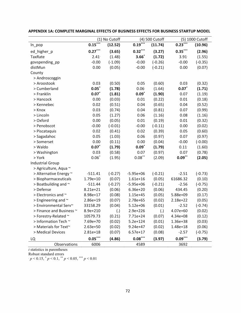
72

APPENDIX 1A: COMPLETE MARGINAL EFFECTS OF BUSINESS EFFECTS FOR BUSINESS STARTUP MODEL

(1) No Cutoff (4) 500 Cutoff (5) 1000 Cutoff ln_pop 0.15*** (12.52) 0.19*** (11.74) 0.23*** (10.96) ed_higher_p 0.27*** (3.65) 0.32*** (3.27) 0.35*** (2.96) TaxRate 2.41. (1.48) 3.66* (1.72) 3.91. (1.55) govspending_pp -0.00 (-1.09) -0.00 (-0.26) -0.00 (-0.35) distMun 0.00 (0.05) -0.00 (-0.21) 0.00 (0.07) County > Androscoggin > Aroostook 0.03 (0.50) 0.05 (0.60) 0.03 (0.32) > Cumberland 0.05* (1.78) 0.06. (1.64) 0.07* (1.71) > Franklin 0.07* (1.81) 0.09* (1.90) 0.07 (1.19) > Hancock 0.00 (0.03) 0.01 (0.22) 0.01 (0.18) > Kennebec 0.02 (0.51) 0.04 (0.65) 0.04 (0.52) > Knox 0.03 (0.74) 0.04 (0.81) 0.07 (0.99) > Lincoln 0.05 (1.27) 0.06 (1.16) 0.08 (1.16) > Oxford 0.00 (0.05) 0.01 (0.19) 0.01 (0.32) > Penobscot -0.00 (-0.01) -0.00 (-0.11) 0.00 (0.02) > Piscataquis 0.02 (0.41) 0.02 (0.39) 0.05 (0.60) > Sagadahoc 0.05 (1.03) 0.06 (0.97) 0.07 (0.97) > Somerset 0.00 (0.11) 0.00 (0.04) -0.00 (-0.00) > Waldo 0.07* (1.79) 0.09* (1.79) 0.11. (1.60) > Washington 0.03 (0.58) 0.07 (0.97) 0.07 (0.78) > York 0.06* (1.95) 0.08** (2.09) 0.09** (2.05) Industrial Group > Agriculture, Aqua ~ > Alternative Energy ~ -511.41 (-0.27) -5.95e+06 (-0.21) -2.51 (-0.73) > Biopharmaceuticals 1.79e+10 (0.07) 1.61e+16 (0.05) 61686.32 (0.10) > Boatbuilding and ~ -511.44 (-0.27) -5.95e+06 (-0.21) -2.56 (-0.75) > Defense 8.21e+21 (0.06) 6.36e+20 (0.06) 434.45 (0.20) > Electronics and ~ 8.98e+17 (0.08) 1.15e+45 (0.05) 5.88e+09 (0.17) > Engineering and ~ 2.86e+19 (0.07) 2.78e+65 (0.02) 2.18e+22 (0.05) > Environmental Serv~ 33158.29 (0.04) 5.12e+06 (0.01) -2.52 (-0.74) > Finance and Business ~ 8.9e+210 (.) 2.9e+226 (.) 4.07e+60 (0.02) > Forestry-Related ~ 10579.73 (0.21) 7.71e+24 (0.07) 4.34e+08 (0.12) > Information Tech ~ 7.69e+70 (0.02) 5.2e+124 (0.01) 1.36e+38 (0.03) > Materials for Text~ 2.63e+50 (0.02) 9.24e+47 (0.02) 1.48e+18 (0.06) > Medical Devices 2.81e+18 (0.07) 6.57e+17 (0.08) -2.57 (-0.75) LQ 0.05*** (4.86) 0.08*** (3.97) 0.09*** (3.79)

Observations 6006 4589 3692 t statistics in parentheses Robust standard errors . p < 0.15, * p < 0.1, ** p < 0.05, *** p < 0.01

73

APPENDIX 2A: COMPLETE MARGINAL EFFECTS OF JOB-MATCHING MODEL

(1) All (2) Female (3) Male NYEARS -0.00 (-1.27) -0.00 (-1.07) -0.00 (-0.51) Marital Status > Married 0.02 (0.86) 0.04. (1.47) -0.01 (-0.46) Highest Degree > Associate's -0.18 (-1.23) 0.00 (.) -0.39* (-1.86) > Doctorate 0.14*** (4.84) 0.13*** (3.16) 0.15*** (4.01) > Masters 0.10*** (5.61) 0.09*** (3.50) 0.11*** (4.36) > Professional 0.19*** (8.78) 0.19*** (7.69) 0.20*** (7.08) UM College > Ed and Human Dev 0.03 (1.32) 0.02 (0.82) 0.04 (1.02) > Engineering 0.03 (1.20) 0.07* (1.80) 0.03 (1.07) > Interdisc -0.05 (-0.71) -0.03 (-0.32) -0.07 (-0.68) > Business -0.04. (-1.50) -0.03 (-0.59) -0.05 (-1.23) > NSFA -0.01 (-0.52) -0.04 (-1.28) 0.01 (0.36) Career Loc Pref > Important 0.07*** (2.84) 0.07** (2.07) 0.06. (1.45) Spouse Loc Pref > Important -0.01 (-0.29) -0.01 (-0.30) 0.01 (0.47) lncountypop 0.03*** (4.03) 0.02 (1.38) 0.05*** (4.12) UNEMP_COLLEGE_P -2.62** (-2.16) -0.10 (-0.06) -4.08** (-2.47) Employment Type > Non Profit 0.10*** (3.87) 0.14*** (3.55) 0.08** (2.03) > Govt 0.09*** (3.47) 0.09** (2.24) 0.10*** (3.16) Occupation > Business Fin ~. 0.30*** (6.47) 0.30*** (5.01) 0.27*** (3.45) > Engineer and Sci~ 0.32*** (6.85) 0.29*** (4.42) 0.32*** (4.11) > Educ and Lib 0.31*** (6.15) 0.29*** (4.86) 0.33*** (3.84) > Healthcare~ 0.22*** (3.48) 0.29*** (4.18) 0.04 (0.28) > Legal, Community~ 0.28*** (5.47) 0.30*** (4.96) 0.24*** (2.70) > Management 0.29*** (6.55) 0.30*** (5.56) 0.27*** (3.48) > Other -0.15* (-1.70) -0.19 (-1.40) -0.14 (-1.15) SOC.LQ 0.04 (1.10) 0.09. (1.60) 0.01 (0.16) Industry > Agr. forresty~ 0.15*** (3.04) 0.20*** (3.54) 0.08 (1.02) > Educ services 0.10** (2.39) 0.09* (1.71) 0.07 (1.11) > Finance and ~ 0.05 (1.33) -0.04 (-0.56) 0.09** (2.01) > Healthcare ~ 0.10** (2.44) 0.11* (1.91) 0.07 (1.15) > Manufacturing 0.16*** (5.18) 0.12* (1.95) 0.17*** (4.86) > Other services 0.02 (0.33) 0.01 (0.15) 0.04 (0.45) > Prof scient~ 0.16*** (5.51) 0.16*** (3.27) 0.16*** (4.53) > Public admin 0.04 (0.70) 0.05 (0.66) 0.03 (0.38) IND.LQ 0.02 (0.97) -0.02 (-0.72) 0.04** (2.23) Observations 1769 841 924 t statistics in parentheses . p < 0.15, * p < 0.1, ** p < 0.05, *** p < 0.01

74

BIOGRAPHY OF THE AUTHOR

Mariya Pominova was born in Donetsk, Ukraine but was raised in the Greater Boston Area after

immigrating to the United States in 2002. She received her Bachelor of Science in Economics from the

University of Maine in 2018 and continued on with her Masters immediately after. Her research

interests in the field have been in macroeconomics, namely the impact of labor market fluctuations have

on regional economic conditions and its policy implications. Mariya is a candidate for a Master of

Science degree in Economics from the University of Maine in May 2020. After graduation, she will be

continuing her work in macroeconomics at the Federal Reserve Board in Washington DC. She is a

candidate for the Master of Science degree in Economics from the University of Maine in May 2020.