Preprint typeset in JHEP style - HYPER VERSION Lent Term, 2017

Applications of Quantum Mechanics

University of Cambridge Part II Mathematical Tripos

David Tong

Department of Applied Mathematics and Theoretical Physics,

Centre for Mathematical Sciences,

Wilberforce Road,

Cambridge, CB3 OBA, UK

http://www.damtp.cam.ac.uk/user/tong/aqm.html

d.tong@damtp.cam.ac.uk

– 1 –

Recommended Books and Resources

This course topics related to di↵erent areas of physics, several of which cannot be

found in traditional quantum textbooks. This is especially true for the condensed

matter aspects of the course, covered in Sections 2, 3 and 4.

• Ashcroft and Mermin, Solid State Physics

• Kittel, Introduction to Solid State Physics

• Steve Simon, Solid State Physics Basics

Ashcroft & Mermin and Kittel are the two standard introductions to condensed matter

physics, both of which go substantially beyond the material covered in this course. I

have a slight preference for the verbosity of Ashcroft and Mermin. The book by Steve

Simon covers only the basics, but does so very well. (An earlier draft can be downloaded

from the course website.)

There are many good books on quantum mechanics. Here’s a selection that I like:

• Gri�ths, Introduction to Quantum Mechanics

An excellent way to ease yourself into quantum mechanics, with uniformly clear expla-

nations. For this course, it covers both approximation methods and scattering.

• Shankar, Principles of Quantum Mechanics

• James Binney and David Skinner, The Physics of Quantum Mechanics

• Weinberg, Lectures on Quantum Mechanics

These are all good books, giving plenty of detail and covering more advanced topics.

Shankar is expansive, Binney and Skinner clear and concise. Weinberg likes his own

notation more than you will like his notation, but it’s worth persevering.

• John Preskill, Course on Quantum Computation

Preskill’s online lecture course has become the default resource for topics on quantum

foundations.

A number of further lecture notes are available on the web. Links can be found on

the course webpage: http://www.damtp.cam.ac.uk/user/tong/aqm.html

Contents

0. Introduction 1

1. Particles in a Magnetic Field 3

1.1 Gauge Fields 3

1.1.1 The Hamiltonian 4

1.1.2 Gauge Transformations 5

1.2 Landau Levels 6

1.2.1 Degeneracy 8

1.2.2 Symmetric Gauge 10

1.2.3 An Invitation to the Quantum Hall E↵ect 11

1.3 The Aharonov-Bohm E↵ect 14

1.3.1 Particles Moving around a Flux Tube 14

1.3.2 Aharonov-Bohm Scattering 16

1.4 Magnetic Monopoles 17

1.4.1 Dirac Quantisation 17

1.4.2 A Patchwork of Gauge Fields 20

1.4.3 Monopoles and Angular Momentum 21

1.5 Spin in a Magnetic Field 23

1.5.1 Spin Precession 25

1.5.2 A First Look at the Zeeman E↵ect 26

2. Band Structure 27

2.1 Electrons Moving in One Dimension 27

2.1.1 The Tight-Binding Model 27

2.1.2 Nearly Free Electrons 33

2.1.3 The Floquet Matrix 40

2.1.4 Bloch’s Theorem in One Dimension 42

2.2 Lattices 47

2.2.1 Bravais Lattices 47

2.2.2 The Reciprical Lattice 53

2.2.3 The Brillouin Zone 56

2.3 Band Structure 58

2.3.1 Bloch’s Theorem 59

2.3.2 Nearly Free Electrons in Three Dimensions 60

– 1 –

2.3.3 Wannier Functions 65

2.3.4 Tight-Binding in Three Dimensions 66

2.3.5 Deriving the Tight-Binding Model 67

3. Electron Dynamics in Solids 74

3.1 Fermi Surfaces 74

3.1.1 Metals vs Insulators 75

3.1.2 The Discovery of Band Structure 80

3.1.3 Graphene 81

3.2 Dynamics of Bloch Electrons 85

3.2.1 Velocity 86

3.2.2 The E↵ective Mass 88

3.2.3 Semi-Classical Equation of Motion 89

3.2.4 Holes 91

3.2.5 Drude Model Again 93

3.3 Bloch Electrons in a Magnetic Field 95

3.3.1 Semi-Classical Motion 95

3.3.2 Cyclotron Frequency 97

3.3.3 Onsager-Bohr-Sommerfeld Quantisation 98

3.3.4 Quantum Oscillations 100

4. Phonons 103

4.1 Lattices in One Dimension 103

4.1.1 A Monotonic Chain 103

4.1.2 A Diatomic Chain 105

4.1.3 Peierls Transition 107

4.1.4 Quantum Vibrations 110

4.2 From Atoms to Fields 114

4.2.1 Phonons in Three Dimensions 115

4.2.2 From Fields to Phonons 116

5. Discrete Symmetries 119

5.1 Parity 119

5.1.1 Parity as a Quantum Number 121

5.1.2 Intrinsic Parity 125

5.2 Time Reversal Invariance 128

5.2.1 Time Evolution is an Anti-Unitary Operator 131

5.2.2 An Example: Spinless Particles 134

– 2 –

5.2.3 Another Example: Spin 136

5.2.4 Kramers Degeneracy 138

6. Approximation Methods 140

6.1 The Variational Method 140

6.1.1 An Upper Bound on the Ground State 140

6.1.2 An Example: The Helium Atom 143

6.1.3 Do Bound States Exist? 147

6.1.4 An Upper Bound on Excited States 152

6.2 WKB 153

6.2.1 The Semi-Classical Expansion 153

6.2.2 A Linear Potential and the Airy Function 157

6.2.3 Bound State Spectrum 161

6.2.4 Bohr-Sommerfeld Quantisation 162

6.2.5 Tunnelling out of a Trap 163

6.3 Changing Hamiltonians, Fast and Slow 166

6.3.1 The Sudden Approximation 166

6.3.2 An Example: Quantum Quench of a Harmonic Oscillator 167

6.3.3 The Adiabatic Approximation 168

6.3.4 Berry Phase 170

6.3.5 An Example: A Spin in a Magnetic Field 173

6.3.6 The Born-Oppenheimer Approximation 176

6.3.7 An Example: Molecules 178

7. Atoms 180

7.1 Hydrogen 181

7.1.1 A Review of the Hydrogen Atom 181

7.1.2 Relativistic Motion 184

7.1.3 Spin-Orbit Coupling and Thomas Precession 187

7.1.4 Zitterbewegung and the Darwin Term 192

7.1.5 Finally, Fine-Structure 194

7.1.6 Hyperfine Structure 195

7.2 Atomic Structure 199

7.2.1 A Closer Look at the Periodic Table 199

7.2.2 Helium and the Exchange Energy 203

7.3 Self-Consistent Field Method 208

7.3.1 The Hartree Method 208

7.3.2 The Slater Determinant 212

– 3 –

7.3.3 The Hartree-Fock Method 214

8. Atoms in Electromagnetic Fields 218

8.1 The Stark E↵ect 218

8.1.1 The Linear Stark E↵ect 219

8.1.2 The Quadratic Stark E↵ect 221

8.1.3 A Little Nazi-Physics History 222

8.2 The Zeeman E↵ect 223

8.2.1 Strong(ish) Magnetic Fields 224

8.2.2 Weak Magnetic Fields 226

8.2.3 The Discovery of Spin 228

8.3 Shine a Light 230

8.3.1 Rabi Oscillations 231

8.3.2 Spontaneous Emission 235

8.3.3 Selection Rules 239

8.4 Photons 241

8.4.1 The Hilbert Space of Photons 241

8.4.2 Coherent States 243

8.4.3 The Jaynes-Cummings Model 245

9. Quantum Foundations 251

9.1 Entanglement 251

9.1.1 The Einstein, Podolsky, Rosen “Paradox” 252

9.1.2 Bell’s Inequality 254

9.1.3 CHSH Inequality 258

9.1.4 Entanglement Between Three Particles 259

9.1.5 The Kochen-Specker Theorem 261

9.2 Entanglement is a Resource 263

9.2.1 The CHSH Game 263

9.2.2 Dense Coding 265

9.2.3 Quantum Teleportation 267

9.2.4 Quantum Key Distribution 270

9.3 Density Matrices 272

9.3.1 The Bloch Sphere 275

9.3.2 Entanglement Revisited 277

9.3.3 Entropy 282

9.4 Measurement 283

9.4.1 Projective Measurements 284

– 4 –

9.4.2 Generalised Measurements 286

9.4.3 The Fate of the State 288

9.5 Open Systems 291

9.5.1 Quantum Maps 291

9.5.2 Decoherence 293

9.5.3 The Lindblad Equation 296

10. Scattering Theory 300

10.1 Scattering in One Dimension 300

10.1.1 Reflection and Transmission Amplitudes 301

10.1.2 Introducing the S-Matrix 306

10.1.3 A Parity Basis for Scattering 307

10.1.4 Bound States 311

10.1.5 Resonances 313

10.2 Scattering in Three Dimensions 317

10.2.1 The Cross-Section 317

10.2.2 The Scattering Amplitude 320

10.2.3 Partial Waves 322

10.2.4 The Optical Theorem 325

10.2.5 An Example: A Hard Sphere and Spherical Bessel Functions 327

10.2.6 Bound States 330

10.2.7 Resonances 334

10.3 The Lippmann-Schwinger Equation 336

10.3.1 The Born Approximation 341

10.3.2 The Yukawa Potential and the Coulomb Potential 342

10.3.3 The Born Expansion 344

10.4 Rutherford Scattering 345

10.4.1 The Scattering Amplitude 346

10.5 Scattering O↵ a Lattice 348

10.5.1 The Bragg Condition 350

10.5.2 The Structure Factor 352

10.5.3 The Debye-Waller Factor 353

– 5 –

Acknowledgements

This course is built on the foundation of previous courses, given in Cambridge by Ron

Horgan and Nick Dorey. I’m supported by the Royal Society.

– 6 –

0. Introduction

Without wishing to overstate the case, the discovery of quantum mechanics is the single

greatest achievement in the history of human civilisation.

Quantum mechanics is an outrageous departure from our classical, comforting, com-

mon sense view of the world. It is more ba✏ing and disturbing than anything dreamt

up by science fiction writers. And yet it is undoubtably the correct description of

the Universe we inhabit and has allowed us to understand Nature with unprecedented

accuracy. In these lectures we will explore some of these developments.

The applications of quantum mechanics are many and various, and vast swathes of

modern physics fall under this rubric. Here we tell only a few of the possible stories,

laying the groundwork for future exploration.

Much of these lectures is devoted to condensed matter physics or, more precisely,

solid state physics. This is the study of “stu↵”, of how the wonderfully diverse prop-

erties of solids can emerge from the simple laws that govern electrons and atoms. We

will develop the basics of the subject, learning how electrons glide through seemingly

impenetrable solids, how their collective motion is described by a Fermi surface, and

how the vibrations of the underlying atoms get tied into bundles of energy known as

phonons. We will learn that electrons in magnetic fields can do strange things, and

start to explore some of the roles that geometry and topology play in quantum physics.

We then move on to atomic physics. Current research in atomic physics is largely

devoted to exquisitely precise manipulation of cold atoms, bending them to our will.

Here, our focus is more old-fashioned and we look only at the basics of the subject,

including the detailed the spectrum of the hydrogen atom, and a few tentative steps

towards understanding the structure of many-electron atoms. We also describe the

various responses of atoms to electromagnetic prodding.

We devote one chapter of these notes to revisiting some of the foundational aspects

of quantum mechanics, starting with the important role played by entanglement as a

way to distinguish between a quantum and classical world. We will provide a more

general view of the basic ideas of states and measurements, as well as an introduction

to the quantum mechanics of open systems.

The final major topic is scattering theory. In the past century, physicists have de-

veloped a foolproof and powerful method to understand everything and anything: you

take the object that you’re interested in and you throw something at it. This technique

was pioneered by Rutherford who used it to understand the structure of the atom. It

– 1 –

was used by Franklin, Crick and Watson to understand the structure of DNA. And,

more recently, it was used at the LHC to demonstrate the existence of the Higgs boson.

In fact, throwing stu↵ at other stu↵ is the single most important experimental method

known to science. It underlies much of what we know about condensed matter physics

and all of what we know about high-energy physics.

In many ways, these lectures are where theoretical physics starts to fracture into

separate sub-disciplines. Yet areas of physics which study systems separated by orders

of magnitude — from the big bang, to stars, to materials, to information, to atoms

and beyond — all rest on a common language and background. The purpose of these

lectures is to build this shared base of knowledge.

– 2 –

1. Particles in a Magnetic Field

The purpose of this chapter is to understand how quantum particles react to magnetic

fields. Before we get to describe quantum e↵ects, we first need to highlight a few of

the more subtle aspects that arise when discussing classical physics in the presence of

a magnetic field.

1.1 Gauge Fields

Recall from our lectures on Electromagnetism that the electric field E(x, t) and mag-

netic fieldB(x, t) can be written in terms a scalar potential �(x, t) and a vector potential

A(x, t),

E = �r�� @A

@tand B = r⇥A (1.1)

Both � andA are referred to as gauge fields. When we first learn electromagnetism, they

are introduced merely as handy tricks to help solve the Maxwell equations. However,

as we proceed through theoretical physics, we learn that they play a more fundamental

role. In particular, they are necessary if we want to discuss a Lagrangian or Hamiltonian

approach to electromagnetism. We will soon see that these gauge fields are quite

indispensable in quantum mechanics.

The Lagrangian for a particle of charge q and mass m moving in a background

electromagnetic fields is

L =1

2mx2 + qx ·A� q� (1.2)

The classical equation of motion arising from this Lagrangian is

mx = q (E+ x⇥B)

This is the Lorentz force law.

Before we proceed I should warn you of a minus sign issue. We will work with

a general charge q. However, many textbooks work with the charge of the electron,

written as q = �e. If this minus sign leans to confusion, you should blame Benjamin

Franklin.

– 3 –

An Example: Motion in a Constant Magnetic Field

We’ll take a constant magnetic field, pointing in the z-direction: B = (0, 0, B). We’ll

take E = 0. The particle is free in the z-direction, with the equation of motion mz = 0.

The more interesting dynamics takes place in the (x, y)-plane where the equations of

motion are

mx = qBy and my = �qBx (1.3)

which has general solution is

x(t) = X +R sin(!B(t� t0

)) and y(t) = Y +R cos(!B(t� t0

))

We see that the particle moves in a circle which, forB > 0 B

Figure 1:

and q > 0, is in a clockwise direction. The cyclotron

frequency is defined by

!B =qB

m(1.4)

The centre of the circle (X, Y ), the radius of the circle R

and the phase t0

are all arbitrary. These are the four integration constants expected in

the solution of two, second order di↵erential equations.

1.1.1 The Hamiltonian

The canonical momentum in the presence of gauge fields is

p =@L

@x= mx+ qA (1.5)

This clearly is not the same as what we naively call momentum, namely mx.

The Hamiltonian is given by

H = x · p� L =1

2m(p� qA)2 + q�

Written in terms of the velocity of the particle, the Hamiltonian looks the same as

it would in the absence of a magnetic field: H = 1

2

mx2 + q�. This is the statement

that a magnetic field does no work and so doesn’t change the energy of the system.

However, there’s more to the Hamiltonian framework than just the value of H. We

need to remember which variables are canonical. This information is encoded in the

Poisson bracket structure of the theory (or, in fancy language, the symplectic structure

on phase space). The fact that x and p are canonical means that

{xi, pj} = �ij with {xi, xj} = {pi, pj} = 0

– 4 –

In the quantum theory, this structure transferred onto commutation relations between

operators, which become

[xi, pj] = i~�ij with [xi, xj] = [pi, pj] = 0

1.1.2 Gauge Transformations

The gauge fields A and � are not unique. We can change them as

�! �� @↵

@tand A ! A+r↵ (1.6)

for any function ↵(x, t). Under these transformations, the electric and magnetic fields

(1.1) remain unchanged, as does the Lagrangian (1.2) and the resulting equations of

motion (1.3). Di↵erent choices of ↵ are said to be di↵erent choices of gauge. We’ll see

some examples below.

The existence of gauge transformations is a redundancy in our description of the

system: fields which di↵er by the transformation (1.6) describe physically identical

configurations. Nothing that we can physically measure can depend on our choice of

gauge. This, it turns out, is a beautifully subtle and powerful restriction. We will start

to explore some of these subtleties in Sections 1.3 and 1.4

The canonical momentum p defined in (1.5) is not gauge invariant: it transforms

as p ! p + qr↵. This means that the numerical value of p can’t have any physical

meaning since it depends on our choice of gauge. In contrast, the velocity of the particle

x and the Hamiltonian H are both gauge invariant, and therefore physical.

The Schrodinger Equation

Finally, we can turn to the quantum theory. We’ll look at the spectrum in the next

section, but first we wish to understand how gauge transformations work. Following

the usual quantisation procedure, we replace the canonical momentum with

p 7! �i~r

The time-dependent Schrodinger equation for a particle in an electric and magnetic

field then takes the form

i~@ @t

= H =1

2m

⇣�i~r� qA

⌘2

+ q� (1.7)

The shift of the kinetic term to incorporate the vector potentialA is sometimes referred

to as minimal coupling.

– 5 –

Before we solve for the spectrum, there are two lessons to take away. The first is that

it is not possible to formulate the quantum mechanics of particles moving in electric

and magnetic fields in terms of E and B alone. We’re obliged to introduce the gauge

fields A and �. This might make you wonder if, perhaps, there is more to A and �

than we first thought. We’ll see the answer to this question in Section 1.3. (Spoiler:

the answer is yes.)

The second lesson follows from looking at how (1.7) fares under gauge transforma-

tions. It is simple to check that the Schrodinger equation transforms covariantly (i.e.

in a nice way) only if the wavefunction itself also transforms with a position-dependent

phase

(x, t) ! eiq↵(x,t)/~ (x, t) (1.8)

This is closely related to the fact that p is not gauge invariant in the presence of a mag-

netic field. Importantly, this gauge transformation does not a↵ect physical probabilities

which are given by | |2.

The simplest way to see that the Schrodinger equation transforms nicely under the

gauge transformation (1.8) is to define the covariant derivatives

Dt =@

@t+

iq

~ � and Di =@

@xi� iq

~ Ai

In terms of these covariant derivatives, the Schrodinger equation becomes

i~Dt = � ~2m

D2 (1.9)

But these covariant derivatives are designed to transform nicely under a gauge trans-

formation (1.6) and (1.8). You can check that they pick up only a phase

Dt ! eiq↵/~ Dt and Di ! eiq↵/~ Di

This ensures that the Schrodinger equation (1.9) transforms covariantly.

1.2 Landau Levels

Our task now is to solve for the spectrum and wavefunctions of the Schrodinger equa-

tion. We are interested in the situation with vanishing electric field, E = 0, and

constant magnetic field. The quantum Hamiltonian is

H =1

2m(p� qA)2 (1.10)

– 6 –

We take the magnetic field to lie in the z-direction, so that B = (0, 0, B). To proceed,

we need to find a gauge potential A which obeys r⇥A = B. There is, of course, no

unique choice. Here we pick

A = (0, xB, 0) (1.11)

This is called Landau gauge. Note that the magnetic field B = (0, 0, B) is invariant

under both translational symmetry and rotational symmetry in the (x, y)-plane. How-

ever, the choice of A is not; it breaks translational symmetry in the x direction (but not

in the y direction) and rotational symmetry. This means that, while the physics will

be invariant under all symmetries, the intermediate calculations will not be manifestly

invariant. This kind of compromise is typical when dealing with magnetic field.

The Hamiltonian (1.10) becomes

H =1

2m

�p2x + (py � qBx)2 + p2z

�Because we have manifest translational invariance in the y and z directions, we have

[py, H] = [pz, H] = 0 and can look for energy eigenstates which are also eigenstates of

py and pz. This motivates the ansatz

(x) = eikyy+ikz

z �(x) (1.12)

Acting on this wavefunction with the momentum operators py = �i~@y and pz = �i~@z,we have

py = ~ky and pz = ~kz

The time-independent Schrodinger equation is H = E . Substituting our ansatz

(1.12) simply replaces py and pz with their eigenvalues, and we have

H (x) =1

2m

hp2x + (~ky � qBx)2 + ~2k2

z

i (x) = E (x)

We can write this as an eigenvalue equation for the equation �(x). We have

H�(x) =

✓E � ~2k2

z

2m

◆�(x)

where H is something very familiar: it’s the Hamiltonian for a harmonic oscillator in

the x direction, with the centre displaced from the origin,

H =1

2mp2x +

m!2

B

2(x� kyl

2

B)2 (1.13)

– 7 –

The frequency of the harmonic oscillator is again the cyloctron frequency !B = qB/m,

and we’ve also introduced a length scale lB. This is a characteristic length scale which

governs any quantum phenomena in a magnetic field. It is called the magnetic length.

lB =

s~qB

To give you some sense for this, in a magnetic field of B = 1 Tesla, the magnetic length

for an electron is lB ⇡ 2.5⇥ 10�8 m.

Something rather strange has happened in the Hamiltonian (1.13): the momentum

in the y direction, ~ky, has turned into the position of the harmonic oscillator in the x

direction, which is now centred at x = kyl2B.

We can immediately write down the energy eigenvalues of (1.13); they are simply

those of the harmonic oscillator

E = ~!B

✓n+

1

2

◆+

~2k2

z

2mn = 0, 1, 2, . . . (1.14)

The wavefunctions depend on three quantum numbers, n 2 N and ky, kz 2 R. They

are

n,k(x, y) ⇠ eikyy+ikz

z Hn(x� kyl2

B)e�(x�k

y

l2B

)

2/2l2B (1.15)

with Hn the usual Hermite polynomial wavefunctions of the harmonic oscillator. The ⇠reflects the fact that we have made no attempt to normalise these these wavefunctions.

The wavefunctions look like strips, extended in the y direction but exponentially

localised around x = kyl2B in the x direction. However, you shouldn’t read too much

into this. As we will see shortly, there is large degeneracy of wavefunctions and by

taking linear combinations of these states we can cook up wavefunctions that have

pretty much any shape you like.

1.2.1 Degeneracy

The dynamics of the particle in the z-direction is una↵ected by the magnetic field

B = (0, 0, B). To focus on the novel physics, let’s restrict to particles with kz = 0. The

energy spectrum then coincides with that of a harmonic oscillator,

En = ~!B

✓n+

1

2

◆(1.16)

– 8 –

In the present context, these are called Landau levels. WeE

k

n=1

n=2

n=3

n=4

n=5

n=0

Figure 2: Landau Levels

see that, in the presence of a magnetic field, the energy levels

of a particle become equally spaced, with the gap between

each level proportional to the magnetic field B. Note that

the energy spectrum looks very di↵erent from a free particle

moving in the (x, y)-plane.

The states in a given Landau level are not unique. In-

stead, there is a huge degeneracy, with many states having

the same energy. We can see this in the form of the wave-

functions (1.15) which, when kz = 0, depend on two quantum numbers, n and ky. Yet

the energy (1.16) is independent of ky.

Let’s determine how large this degeneracy of states is. To do so, we need to restrict

ourselves to a finite region of the (x, y)-plane. We pick a rectangle with sides of lengths

Lx and Ly. We want to know how many states fit inside this rectangle.

Having a finite size Ly is like putting the system in a box in the y-direction. The

wavefunctions must obey

(x, y + Ly, z) = (x, y, z) ) eikyLy = 1

This means that the momentum ky is quantised in units of 2⇡/Ly.

Having a finite size Lx is somewhat more subtle. The reason is that, as we mentioned

above, the gauge choice (1.11) does not have manifest translational invariance in the

x-direction. This means that our argument will be a little heuristic. Because the

wavefunctions (1.15) are exponentially localised around x = kyl2B, for a finite sample

restricted to 0 x Lx we would expect the allowed ky values to range between

0 ky Lx/l2B. The end result is that the number of states in each Landau level is

given by

N =Ly

2⇡

Z Lx

/l2B

0

dk =LxLy

2⇡l2B=

qBA

2⇡~ (1.17)

where A = LxLy is the area of the sample. Strictly speaking, we should take the integer

part of the answer above.

The degeneracy (1.17) is very very large. Throwing in some numbers, there are

around 1010 degenerate states per Landau level for electrons in a region of area A =

1 cm2 in a magnetic field B ⇠ 0.1 T . This large degeneracy ultimately, this leads to

an array of dramatic and surprising physics.

– 9 –

1.2.2 Symmetric Gauge

It is worthwhile to repeat the calculations above using a di↵erent gauge choice. This

will give us a slightly di↵erent perspective on the physics. A natural choice is symmetric

gauge

A = �1

2x⇥B =

B

2(�y, x, 0) (1.18)

This choice of gauge breaks translational symmetry in both the x and the y directions.

However, it does preserve rotational symmetry about the origin. This means that

angular momentum is now a good quantum number to label states.

In this gauge, the Hamiltonian is given by

H =1

2m

"✓px +

qBy

2

◆2

+

✓py �

qBx

2

◆2

+ p2z

#

= � ~22m

r2 +qB

2mLz +

q2B2

8m(x2 + y2) (1.19)

where we’ve introduced the angular momentum operator

Lz = xpy � ypx

We’ll again restrict to motion in the (x, y)-plane, so we focus on states with kz = 0.

It turns out that complex variables are particularly well suited to describing states in

symmetric gauge, in particular in the lowest Landau level with n = 0. We define

w = x+ iy and w = x� iy

Correspondingly, the complex derivatives are

@ =1

2

✓@

@x� i

@

@y

◆and @ =

1

2

✓@

@x+ i

@

@y

◆which obey @w = @w = 1 and @w = @w = 0. The Hamiltonian, restricted to states

with kz = 0, is then given by

H = �2~2m@@ � !B

2Lz +

m!2

B

8ww

where now

Lz = ~(w@ � w@)

– 10 –

It is simple to check that the states in the lowest Landau level take the form

0

(w, w) = f(w)e�|w|2/4l2B

for any holomorphic function f(w). These all obey

H 0

(w, w) =~!B

2 0

(w, w)

which is the statement that they lie in the lowest Landau level with n = 0. We can

further distinguish these states by requiring that they are also eigenvalues of Lz. These

are satisfied by the monomials,

0

= wMe�|w|2/4l2B ) Lz 0

= ~M 0

(1.20)

for some positive integer M .

Degeneracy Revisited

In symmetric gauge, the profiles of the wavefunctions (1.20) form concentric rings

around the origin. The higher the angular momentum M , the further out the ring.

This, of course, is very di↵erent from the strip-like wavefunctions that we saw in Landau

gauge (1.15). You shouldn’t read too much into this other than the fact that the profile

of the wavefunctions is not telling us anything physical as it is not gauge invariant.

However, it’s worth revisiting the degeneracy of states in symmetric gauge. The

wavefunction with angular momentum M is peaked on a ring of radius r =p2MlB.

This means that in a disc shaped region of area A = ⇡R2, the number of states is

roughly (the integer part of)

N = R2/2l2B = A/2⇡l2B =qBA

2⇡~which agrees with our earlier result (1.17).

1.2.3 An Invitation to the Quantum Hall E↵ect

Take a system with some fixed number of electrons, which are restricted to move in

the (x, y)-plane. The charge of the electron is q = �e. In the presence of a magnetic

field, these will first fill up the N = eBA/2⇡~ states in the n = 0 lowest Landau level.

If any are left over they will then start to fill up the n = 1 Landau level, and so on.

Now suppose that we increase the magnetic field B. The number of states N housed

in each Landau level will increase, leading to a depletion of the higher Landau levels.

At certain, very special values of B, we will find some number of Landau levels that

are exactly filled. However, generically there will be a highest Landau level which is

only partially filled.

– 11 –

Figure 3: The integer quantum Hall ef-

fect.

Figure 4: The fractional quantum Hall

e↵ect.

This successive depletion of Landau levels gives rise to a number of striking signatures

in di↵erent physical quantities. Often these quantities oscillate, or jump discontinuously

as the number of occupied Landau levels varies. One particular example is the de Haas

van Alphen oscillations seen in the magnetic susceptibility which we describe in Section

3.3.4. Another example is the behaviour of the resistivity ⇢. This relates the current

density J = (Jx, Jy) to the applied electric field E = (Ex, Ey),

E = ⇢J

In the presence of an applied magnetic field B = (0, 0, B), the electrons move in circles.

This results in components of the current which are both parallel and perpendicular to

the electric field. This is modelled straightforwardly by taking ⇢ to be a matrix

⇢ =

⇢xx ⇢xy

�⇢xy ⇢xx

!where the form of the matrix follows from rotational invariance. Here ⇢xx is called the

longitudinal resistivity while ⇢xy is called the Hall resistivity.

In very clean samples, in strong magnetic fields, both components of the resistivity

exhibit very surprising behaviour. This is shown in the left-hand figure above. The

Hall resistivity ⇢xy increases with B by forming a series of plateaux, on which it takes

values

⇢xy =2⇡~e2

1

⌫⌫ 2 N

The value of ⌫ (which is labelled i = 2, 3, . . . in the data shown above) is measured

to be an integer to extraordinary accuracy — around one part in 109. Meanwhile,

– 12 –

the longitudinal resistivity vanishes when ⇢xy lies on a plateaux, but spikes whenever

there is a transition between di↵erent plateaux. This phenomenon, called the integer

Quantum Hall E↵ect, was discovered by Klaus von Klitzing in 1980. For this, he was

awarded the Nobel prize in 1985.

It turns out that the integer quantum Hall e↵ect is a direct consequence of the

existence of discrete Landau levels. The plateaux occur when precisely ⌫ 2 Z+ Landau

levels are filled. Of course, we’re very used to seeing integers arising in quantum

mechanics — this, after all, is what the “quantum” in quantum mechanics means.

However, the quantisation of the resistivity ⇢xy is something of a surprise because

this is a macroscopic quantity, involving the collective behaviour of many trillions of

electrons, swarming through a hot and dirty system. A full understanding of the integer

quantum Hall e↵ect requires an appreciation of how the mathematics of topology fits

in with quantum mechanics. David Thouless (and, to some extent, Duncan Haldane)

were awarded the 2016 Nobel prize for understanding the underlying role of topology

in this system.

Subsequently it was realised that similar behaviour also happens when Landau levels

are partially filled. However, it doesn’t occur for any filling, but only very special

values. This is referred to as the fractional quantum Hall e↵ect. The data is shown

in the right-hand figure. You can see clear plateaux when the lowest Landau level has

⌫ = 1

3

of its states filled. There is another plateaux when ⌫ = 2

5

of the states are

filled, followed by a bewildering pattern of further plateaux, all of which occur when ⌫

is some rational number. This was discovered by Tsui and Stormer in 1982. It called

the Fractional Quantum Hall E↵ect. The 1998 Nobel prize was awarded to Tsui and

Stormer, together with Laughlin who pioneered the first theoretical ideas to explain

this behaviour.

The fractional quantum Hall e↵ect cannot be explained by treating the electrons

as free. Instead, it requires us to take interactions into account. We have seen that

each Landau level has a macroscopically large degeneracy. This degeneracy is lifted by

interactions, resulting in a new form of quantum liquid which exhibits some magical

properties. For example, in this state of matter the electron — which, of course,

is an indivisible particle — can split into constituent parts! The ⌫ = 1

3

state has

excitations which carry 1/3 of the charge of an electron. In other quantum Hall states,

the excitations have charge 1/5 or 1/4 of the electron. These particles also have a

number of other, even stranger properties to do with their quantum statistics and

there is hope that these may underly the construction of a quantum computer.

– 13 –

We will not delve into any further details of the quantum Hall e↵ect. Su�ce to say

that it is one of the richest and most beautiful subjects in theoretical physics. You can

find a fuller exploration of these ideas in the lecture notes devoted to the Quantum

Hall E↵ect.

1.3 The Aharonov-Bohm E↵ect

In our course on Electromagnetism, we learned that the gauge potential Aµ is unphys-

ical: the physical quantities that a↵ect the motion of a particle are the electric and

magnetic fields. Yet we’ve seen above that we cannot formulate quantum mechanics

without introducing the gauge fields A and �. This might lead us to wonder whether

there is more to life than E and B alone. In this section we will see that things are,

indeed, somewhat more subtle.

1.3.1 Particles Moving around a Flux Tube

Consider the set-up shown in the figure. We have a solenoid

B=0

B

Figure 5:

of area A, carrying magnetic field B = (0, 0, B) and therefore

magnetic flux � = BA. Outside the solenoid the magnetic

field is zero. However, the vector potential is not. This fol-

lows from Stokes’ theorem which tells us that the line integral

outside the solenoid is given byIA · dx =

ZB · dS = �

This is simply solved in cylindrical polar coordinates by

A� =�

2⇡r

Now consider a charged quantum particle restricted to lie in a ring of radius r outside the

solenoid. The only dynamical degree of freedom is the angular coordinate � 2 [0, 2⇡).

The Hamiltonian is

H =1

2m(p� � qA�)

2 =1

2mr2

✓�i~ @

@�� q�

2⇡

◆2

We’d like to see how the presence of this solenoid a↵ects the particle. The energy

eigenstates are simply

=1p2⇡r

ein� n 2 Z (1.21)

– 14 –

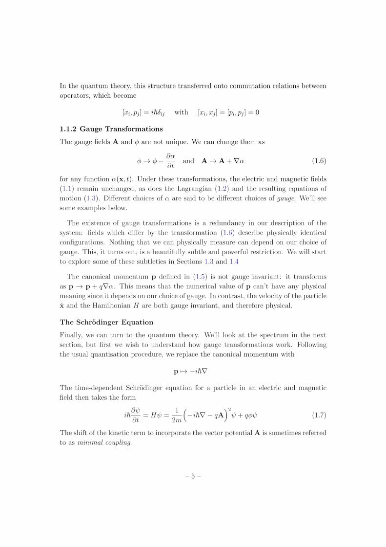
Φ

E

n=1 n=2n=0

Figure 6: The energy spectrum for a particle moving around a solenoid.

where the requirement that is single valued around the circle means that we must

take n 2 Z. Plugging this into the time independent Schrodinger equation H = E ,

we find the spectrum

E =1

2mr2

✓~n� q�

2⇡

◆2

=~2

2mr2

✓n� �

�0

◆2

n 2 Z

where we’ve defined the quantum of flux �0

= 2⇡~/q. (Usually this quantum of flux

is defined using the electron charge q = �e, with the minus signs massaged so that

�0

⌘ 2⇡~/e > 0.)

Note that if � is an integer multiple of �0

, then the spectrum is una↵ected by the

solenoid. But if the flux in the solenoid is not an integral multiple of �0

— and there is

no reason that it should be — then the spectrum gets shifted. We see that the energy

of the particle knows about the flux � even though the particle never goes near the

region with magnetic field. The resulting energy spectrum is shown in Figure 6.

There is a slightly di↵erent way of looking at this result. Away from the solenoid,

the gauge field is a total divergence

A = r↵ with ↵ =��

2⇡

This means that we can try to remove it by redefining the wavefunction to be

! = exp

✓�iq↵

~

◆ = exp

✓�iq�

2⇡~ �

◆

However, there is an issue: the wavefunction should be single-valued. This, after all,

is how we got the quantisation condition n 2 Z in (1.21). This means that the gauge

transformation above is allowed only if � is an integer multiple of �0

= 2⇡~/q. Only

in this case is the particle una↵ected by the solenoid. The obstacle arises from the fact

that the wavefunction of the particle winds around the solenoid. We see here the first

glimpses of how topology starts to feed into quantum mechanics.

– 15 –

1.3.2 Aharonov-Bohm Scattering

The fact that a quantum particle can be a↵ected by A

φ

P

1P

2

Figure 7:

even when restricted to regions where B = 0 was first

pointed out by Aharonov and Bohm in a context which

is closely related to the story above. They revisited the

famous double-slit experiment, but now with a twist:

a solenoid carrying flux � is hidden behind the wall.

This set-up is shown in the figure below. Once again,

the particle is forbidden from going near the solenoid.

Nonetheless, the presence of the magnetic flux a↵ects

the resulting interference pattern, shown as the dotted line in the figure.

Consider a particle that obeys the free Schrodinger equation,

1

2m

⇣� i~r� qA

⌘2

= E

We can formally remove the gauge field by writing

(x) = exp

✓iq

~

Zx

A(x0) · dx0◆�(x)

where the integral is over any path. Crucially, however, in the double-slit experiment

there are two paths, P1

and P2

. The phase picked up by the particle due to the gauge

field di↵ers depending on which path is taken. The phase di↵erence is given by

�✓ =q

~

ZP1

A · dx� q

~

ZP2

A · dx =q

~

IA · dx =

q

~

ZB · dS

Note that neither the phase arising from path P1

, nor the phase arising from path P2

, is

gauge invariant. However, the di↵erence between the two phases is gauge invariant. As

we see above, it is given by the flux through the solenoid. This is the Aharonov-Bohm

phase, eiq�/~, an extra contribution that arises when charged particles move around

magnetic fields.

The Aharonov-Bohm phase manifests in the interference pattern seen on the screen.

As � is changed, the interference pattern shifts, an e↵ect which has been experimentally

observed. Only when � is an integer multiple of �0

is the particle unaware of the

presence of the solenoid.

– 16 –

1.4 Magnetic Monopoles

A magnetic monopole is a hypothetical object which emits a radial magnetic field of

the form

B =gr

4⇡r2)

ZdS ·B = g (1.22)

Here g is called the magnetic charge.

We learned in our first course on Electromagnetism that magnetic monopoles don’t

exist. First, and most importantly, they have never been observed. Second there’s a

law of physics which insists that they can’t exist. This is the Maxwell equation

r ·B = 0

Third, this particular Maxwell equation would appear to be non-negotiable. This is

because it follows from the definition of the magnetic field in terms of the gauge field

B = r⇥A ) r ·B = 0

Moreover, as we’ve seen above, the gauge field A is necessary to describe the quantum

physics of particles moving in magnetic fields. Indeed, the Aharonov-Bohm e↵ect tells

us that there is non-local information stored in A that can only be detected by particles

undergoing closed loops. All of this points to the fact that we would be wasting our

time discussing magnetic monopoles any further.

Happily, there is a glorious loophole in all of these arguments, first discovered by

Dirac, and magnetic monopoles play a crucial role in our understanding of the more

subtle e↵ects in gauge theories. The essence of this loophole is that there is an ambiguity

in how we define the gauge potentials. In this section, we will see how this arises.

1.4.1 Dirac Quantisation

It turns out that not any magnetic charge g is compatible with quantum mechanics.

Here we present several di↵erent arguments for the allowed values of g.

We start with the simplest and most physical of these arguments. Suppose that a

particle with charge q moves along some closed path C in the background of some gauge

potential A(x). Then, upon returning to its initial starting position, the wavefunction

of the particle picks up a phase

! eiq↵/~ with ↵ =

IC

A · dx (1.23)

This is the Aharonov-Bohm phase described above.

– 17 –

B

S

C

C

S’

Figure 8: Integrating over S... Figure 9: ...or over S0.

The phase of the wavefunction is not an observable quantity in quantum mechanics.

However, as we described above, the phase in (1.23) is really a phase di↵erence. We

could, for example, place a particle in a superposition of two states, one of which stays

still while the other travels around the loop C. The subsequent interference will depend

on the phase eiq↵/~, just like in the Aharonov-Bohm e↵ect.

Let’s now see what this has to do with magnetic monopoles. We place our particle,

with electric charge q, in the background of a magnetic monopole with magnetic charge

g. We keep the magnetic monopole fixed, and let the electric particle undergo some

journey along a path C. We will ask only that the path C avoids the origin where the

magnetic monopole is sitting. This is shown in the left-hand panel of the figure. Upon

returning, the particle picks up a phase eiq↵/~ with

↵ =

IC

A · dx =

ZS

B · dS

where, as shown in the figure, S is the area enclosed by C. Using the fact thatRS

2 B ·dS = g, if the surface S makes a solid angle ⌦, this phase can be written as

↵ =⌦g

4⇡

However, there’s an ambiguity in this computation. Instead of integrating over S, it

is equally valid to calculate the phase by integrating over S 0, shown in the right-hand

panel of the figure. The solid angle formed by S 0 is ⌦0 = 4⇡ � ⌦. The phase is then

given by

↵0 = �(4⇡ � ⌦)g

4⇡

where the overall minus sign comes because the surface S 0 has the opposite orientationto S. As we mentioned above, the phase shift that we get in these calculations is

– 18 –

observable: we can’t tolerate di↵erent answers from di↵erent calculations. This means

that we must have eiq↵/~ = eiq↵0/~. This gives the condition

qg = 2⇡~n with n 2 Z (1.24)

This is the famous Dirac quantisation condition. The smallest such magnetic charge

has n = 1. It coincides with the quantum of flux, g = �0

= 2⇡~/q.

Above we worked with a single particle of charge q. Obviously, the same argument

must hold for any other particle of charge q0. There are two possibilities. The first is

that all particles carry charge that is an integer multiple of some smallest unit. In this

case, it’s su�cient to impose the Dirac quantisation condition (1.24) where q is the

smallest unit of charge. For example, in our world we should take q = ±e to be the

electron or proton charge (or, if we look more closely in the Standard Model, we might

choose to take q = �e/3, the charge of the down quark).

The second possibility is that the particles carry electric charges which are irrational

multiples of each other. For example, there may be a particle with charge q and another

particle with chargep2q. In this case, no magnetic monopoles are allowed.

It’s sometimes said that the existence of a magnetic monopole would imply the

quantisation of electric charges. This, however, has it backwards. (It also misses the

point that we have a wonderful explanation of the quantisation of charges from the

story of anomaly cancellation in the Standard Model.) There are two possible groups

that could underly gauge transformations in electromagnetism. The first is U(1); this

has integer valued charges and admits magnetic monopoles. The second possibility is

R; this has irrational electric charges and forbids monopoles. All the evidence in our

world points to the fact that electromagnetism is governed by U(1) and that magnetic

monopoles should exist.

Above we looked at an electrically charged particle moving in the background of

a magnetically charged particle. It is simple to generalise the discussion to particles

that carry both electric and magnetic charges. These are called dyons. For two dyons,

with charges (q1

, g1

) and (q2

, g2

), the generalisation of the Dirac quantisation condition

requires

q1

g2

� q2

g1

2 2⇡~Z

This is sometimes called the Dirac-Zwanziger condition.

– 19 –

1.4.2 A Patchwork of Gauge Fields

The discussion above shows how quantum mechanics constrains the allowed values of

magnetic charge. It did not, however, address the main obstacle to constructing a

magnetic monopole out of gauge fields A when the condition B = r⇥A would seem

to explicitly forbid such objects.

Let’s see how to do this. Our goal is to write down a configuration of gauge fields

which give rise to the magnetic field (1.22) of a monopole which we will place at the

origin. However, we will need to be careful about what we want such a gauge field to

look like.

The first point is that we won’t insist that the gauge field is well defined at the origin.

After all, the gauge fields arising from an electron are not well defined at the position of

an electron and it would be churlish to require more from a monopole. This fact gives

us our first bit of leeway, because now we need to write down gauge fields on R3/{0},as opposed to R3 and the space with a point cut out enjoys some non-trivial topology

that we will make use of.

Consider the following gauge connection, written in spherical polar coordinates

AN� =

g

4⇡r

1� cos ✓

sin ✓(1.25)

The resulting magnetic field is

B = r⇥A =1

r sin ✓

@

@✓(AN

� sin ✓) r� 1

r

@

@r(rAN

� )✓

Substituting in (1.25) gives

B =gr

4⇡r2(1.26)

In other words, this gauge field results in the magnetic monopole. But how is this

possible? Didn’t we learn in kindergarten that if we can write B = r ⇥ A thenRdS ·B = 0? How does the gauge potential (1.25) manage to avoid this conclusion?

The answer is that AN in (1.25) is actually a singular gauge connection. It’s not just

singular at the origin, where we’ve agreed this is allowed, but it is singular along an

entire half-line that extends from the origin to infinity. This is due to the 1/ sin ✓ term

which diverges at ✓ = 0 and ✓ = ⇡. However, the numerator 1� cos ✓ has a zero when

✓ = 0 and the gauge connection is fine there. But the singularity along the half-line

✓ = ⇡ remains. The upshot is that this gauge connection is not acceptable along the

line of the south pole, but is fine elsewhere. This is what the superscript N is there to

remind us: we can work with this gauge connection s long as we keep north.

– 20 –

Now consider a di↵erent gauge connection

AS� = � g

4⇡r

1 + cos ✓

sin ✓(1.27)

This again gives rise to the magnetic field (1.26). This time it is well behaved at ✓ = ⇡,

but singular at the north pole ✓ = 0. The superscript S is there to remind us that this

connection is fine as long as we keep south.

At this point, we make use of the ambiguity in the gauge connection. We are going

to take AN in the northern hemisphere and AS in the southern hemisphere. This is

allowed because the two gauge potentials are the same up to a gauge transformation,

A ! A + r↵. Recalling the expression for r↵ in spherical polars, we find that for

✓ 6= 0, ⇡, we can indeed relate AN� and AS

� by a gauge transformation,

AN� = AS

� +1

r sin ✓@�↵ where ↵ =

g�

2⇡(1.28)

However, there’s still a question remaining: is this gauge transformation allowed? The

problem is that the function ↵ is not single valued: ↵(� = 2⇡) = ↵(� = 0) + g. And

this should concern us because, as we’ve seen in (1.8), the gauge transformation also

acts on the wavefunction of a quantum particle

! eiq↵/~

There’s no reason that we should require the gauge transformation ! to be single-

valued, but we do want the wavefunction to be single-valued. This holds for the

gauge transformation (1.28) provided that we have

qg = 2⇡~n with n 2 Z

This, of course, is the Dirac quantisation condition (1.24).

Mathematically, we have constructed of a topologically non-trivial U(1) bundle over

the S2 surrounding the origin. In this context, the integer n is called the first Chern

number.

1.4.3 Monopoles and Angular Momentum

Here we provide yet another derivation of the Dirac quantisation condition, this time

due to Saha. The key idea is that the quantisation of magnetic charge actually follows

from the more familiar quantisation of angular momentum. The twist is that, in the

presence of a magnetic monopole, angular momentum isn’t quite what you thought.

– 21 –

To set the scene, let’s go back to the Lorentz force law

dp

dt= q x⇥B

with p = mx. Recall from our discussion in Section 1.1.1 that p defined here is not

the canonical momentum, a fact which is hiding in the background in the following

derivation. Now let’s consider this equation in the presence of a magnetic monopole,

with

B =g

4⇡

r

r3

The monopole has rotational symmetry so we would expect that the angular momen-

tum, x⇥ p, is conserved. Let’s check:

d(x⇥ p)

dt= x⇥ p+ x⇥ p = x⇥ p = qx⇥ (x⇥B)

=qg

4⇡r3x⇥ (x⇥ x) =

qg

4⇡

✓x

r� rx

r2

◆=

d

dt

⇣ qg4⇡

r⌘

We see that in the presence of a magnetic monopole, the naiveL

θ

Figure 10:

angular momentum x ⇥ p is not conserved! However, as we also

noticed in the lectures on Classical Dynamics (see Section 4.3.2),

we can easily write down a modified angular momentum that is

conserved, namely

L = x⇥ p� qg

4⇡r

The extra term can be thought of as the angular momentum stored

in E ⇥B. The surprise is that the system has angular momentum

even when the particle doesn’t move.

Before we move on, there’s a nice and quick corollary that we can draw from this.

The angular momentum vector L does not change with time. But the angle that the

particle makes with this vector is

L · r = � qg

4⇡= constant

This means that the particle moves on a cone, with axis L and angle cos ✓ = �qg/4⇡L.

– 22 –

So far, our discussion has been classical. Now we invoke some simple quantum

mechanics: the angular momentum should be quantised. In particular, the angular

momentum in the z-direction should be Lz 2 1

2

~Z. Using the result above, we have

qg

4⇡=

1

2~n ) qg = 2⇡~n with n 2 Z

Once again, we find the Dirac quantisation condition.

1.5 Spin in a Magnetic Field

As we’ve seen in previous courses, particles often carry an intrinsic angular momentum

called spin S. This spin is quantised in half-integer units. For examples, electrons have

spin 1

2

and their spin operator is written in terms of the Pauli matrices �,

S =~2�

Importantly, the spin of any particle couples to a background magnetic field B. The

key idea here is that the intrinsic spin acts like a magnetic moment m which couples

to the magnetic field through the Hamiltonian

H = �m ·B

The question we would like to answer is: what magnetic moment m should we associate

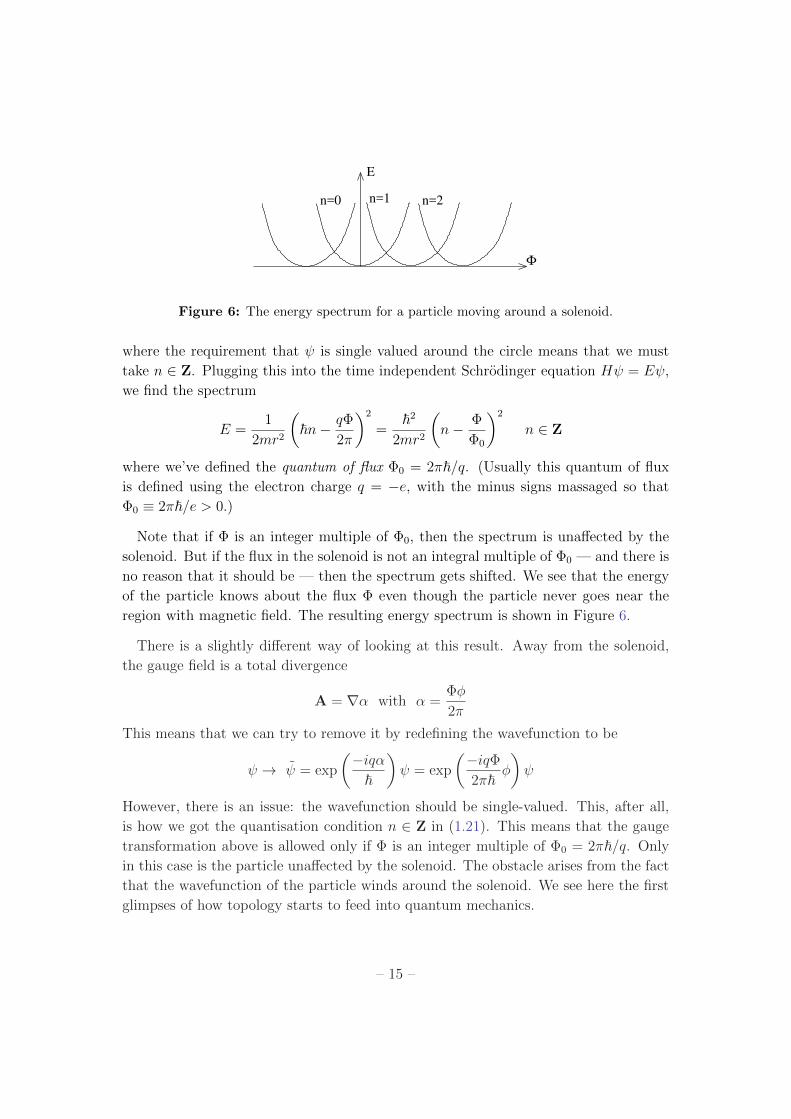
with spin?

A full answer to this question would require an ex-

r

qv

Figure 11:

tended detour into the Dirac equation. Here we pro-

vide only some basic motivation. First consider a par-

ticle of charge q moving with velocity v around a circle

of radius r as shown in the figure. From our lectures on

Electromagnetism, we know that the associated magnetic

moment is given by

m = �q

2r⇥ v =

q

2mL

where L = mr⇥v is the orbital angular momentum of the particle. Indeed, we already

saw the resulting coupling H = �(q/2m)L ·B in our derivation of the Hamiltonian in

symmetric gauge (1.19).

– 23 –

Since the spin of a particle is another contribution to the angular momentum, we

might anticipate that the associated magnetic moment takes the form

m = gq

2mS

where g is some dimensionless number. (Note: g is unrelated to the magnetic charge

that we discussed in the previous section!) This, it turns out, is the right answer.

However, the value of g depends on the particle under consideration. The upshot is

that we should include a term in the Hamiltonian of the form

H = �gq

2mS ·B (1.29)

The g-factor

For fundamental particles with spin 1

2

— such as the electron — there is a long and

interesting history associated to determining the value of g. For the electron, this was

first measured experimentally to be

ge = 2

Soon afterwards, Dirac wrote down his famous relativistic equation for the electron.

One of its first successes was the theoretical prediction ge = 2 for any spin 1

2

particle.

This means, for example, that the neutrinos and quarks also have g = 2.

This, however, was not the end of the story. With the development of quantum field

theory, it was realised that there are corrections to the value ge = 2. These can be

calculated and take the form of a series expansion, starting with

ge = 2⇣1 +

↵

2⇡+ . . .

⌘⇡ 2.00232

where ↵ = e2/4⇡✏0

~c ⇡ 1/137 is the dimensionless fine structure constant which char-

acterises the strength of the Coulomb force. The most accurate experimental measure-

ment of the electron magnetic moment now yields the result

ge ⇡ 2.00231930436182± 2.6⇥ 10�13

Theoretical calculations agree to the first ten significant figures or so. This is the most

impressive agreement between theory and experiment in all of science! Beyond that,

the value of ↵ is not known accurately enough to make a comparison. Indeed, now

the measurement of the electron magnetic moment is used to define the fine structure

constant ↵.

– 24 –

While all fundamental spin 1

2

particles have g ⇡ 2, this does not hold for more

complicated objects. For example, the proton has

gp ⇡ 5.588

while the neutron — which of course, is a neutral particle, but still carries a magnetic

moment — has

gn ⇡ �3.823

where, because the neutron is neutral, the charge q = e is used in the formula (1.29).

These measurements were one of the early hints that the proton and neutron are com-

posite objects.

1.5.1 Spin Precession

Consider a constant magnetic field B = (0, 0, B). We would like to understand how

this a↵ects the spin of an electron. We’ll take ge = 2. We write the electric charge of

the electron as q = �e so the Hamiltonian is

H =e~2m

� ·B

The eigenstates are simply the spin-up |" i and spin-down |# i states in the z-direction.

They have energies

H|" i = ~!B

2|" i and H|# i = �~!B

2|# i

where !B = eB/m is the cyclotron frequency which appears throughout this chapter.

What happens if we do not sit in an energy eigenstate. A

ωB

B

S

Figure 12:

general spin state can be expressed in spherical polar coordinates

as

| (✓,�)i = cos(✓/2)|" i+ ei� sin(✓/2)|# i

As a check, note that | (✓ = ⇡/2,�)i is an eigenstate of �x when

� = 0, ⇡ and an eigenstate of �y when � = ⇡/2, 3⇡/2 as it

should be. The evolution of this state is determined by the time-

dependent Schrodinger equation

i~@| i@t

= H| i

– 25 –

which is easily solved to give

| (✓,�; t)i = ei!B

t/2hcos(✓/2)|" i+ ei(��!

B

t) sin(✓/2)|# ii

We see that the e↵ect of the magnetic field is to cause the spin to precess about the B

axis, as shown in the figure.

1.5.2 A First Look at the Zeeman E↵ect

The Zeeman e↵ect describes the splitting of atomic energy levels in the presence of a

magnetic field. Consider, for example, the hydrogen atom with Hamiltonian

H = � ~22m

r2 � 1

4⇡✏0

e2

r

The energy levels are given by

En = �↵2mc2

2

1

n2

n 2 Z

where ↵ is the fine structure constant. Each energy level has a degeneracy of states.

These are labelled by the angular momentum l = 0, 1, . . . , n� 1 and the z-component

of angular momentum ml = �l, . . . ,+l. Furthermore, each electron carries one of two

spin states labelled by ms = ±1

2

. This results in a degeneracy given by

Degeneracy = 2n�1Xl=0

(2l + 1) = 2n2

Now we add a magnetic fieldB = (0, 0, B). As we have seen, this results in perturbation

to the Hamiltonian which, to leading order in B, is given by

�H =e

2m(L+ geS) ·B

In the presence of such a magnetic field, the degeneracy of the states is split. The

energy levels now depend on the quantum numbers n, ml and ms and are given by

En,m,s = En +e

2m(ml + 2ms)B

The Zeeman e↵ect is described in more detail in Section 8.2.

– 26 –